Université Grenoble AlpesMaster 2 Statistiques et Science des données

Rapport de stage

Conceptually correct and algorithmicallyefficient pruning and allocation procedures

in statistical LUCC modelling

du 1er mars au 31 juillet 2019Équipe STEEP – Inria Grenoble

Élève :François-Rémi Mazy

Encadrants :Pierre-Yves Longaretti (Inria)

Rémy Drouilhet (UGA)

August 26, 2019

ContentsContexte du travail effectué 2

1 Introduction 31.1 Generalities . . . . . . . . . . . . . . . . . . . . . . . . . . . . . . . . . . . . . . . . 31.2 Spatially explicit models architecture . . . . . . . . . . . . . . . . . . . . . . . . . . 31.3 Models limits and work introduction . . . . . . . . . . . . . . . . . . . . . . . . . . 4

2 Notation and definitions 62.1 Pixel characterization parameters . . . . . . . . . . . . . . . . . . . . . . . . . . . . 62.2 Justification elements of the probabilistic approach in the LUCC modeling . . . . . 7

3 A case study: the SCoT of Grenoble 9

4 Calibration through explanatory variables 104.1 Probabilities in the limit of statistical independence of explanatory variables . . . . 104.2 Dinamica weights of evidence . . . . . . . . . . . . . . . . . . . . . . . . . . . . . . 124.3 Imperfect closure . . . . . . . . . . . . . . . . . . . . . . . . . . . . . . . . . . . . . 12

5 Pruning and currently used allocation methods 135.1 Position of the problem . . . . . . . . . . . . . . . . . . . . . . . . . . . . . . . . . 135.2 Summary of Dinamica pruning and allocation strategies involving patches . . . . . 135.3 Defining conceptually correct pruning . . . . . . . . . . . . . . . . . . . . . . . . . 15

6 New land use change allocation algorithm 176.1 Calibration and allocation scenario . . . . . . . . . . . . . . . . . . . . . . . . . . . 176.2 Generalized acceptation rejection test . . . . . . . . . . . . . . . . . . . . . . . . . 176.3 Allocation algorithm . . . . . . . . . . . . . . . . . . . . . . . . . . . . . . . . . . . 18

7 Islands and expansions allocation procedures 217.1 Calibration . . . . . . . . . . . . . . . . . . . . . . . . . . . . . . . . . . . . . . . . 217.2 Island design process . . . . . . . . . . . . . . . . . . . . . . . . . . . . . . . . . . . 227.3 Expansion design process . . . . . . . . . . . . . . . . . . . . . . . . . . . . . . . . 237.4 Patch design implementation within the allocation algorithm . . . . . . . . . . . . 24

8 Conclusion 26

1

Contexte du travail effectuéJ’ai pris contact en avril 2018 avec l’équipe STEEP du centre Inria de Grenoble et nous avonsrapidement monté un projet de doctorat portant sur la modélisations du changement d’usage dessols. Nous nous sommes alors donné un an pour trouver un financement de thèse et dans ce lapsde temps il a été convenu que je suive un master 2 de statistiques afin de compléter ma formationinitiale d’ingénieur dans ce domaine. Le présent document rapporte mon travail effectué dansle cadre du stage de master 2 Statistiques et Sciences des Données (M2 SSD) de l’UniversitéGrenoble Alpes réalisé de mars à juillet 2019. Nous avons finalement obtenu en juin 2019 unebourse de thèse entièrement financée par l’Inria.

Ce stage constitue donc une entrée en matière à ce travail de thèse qui s’effectuera sur les troisprochaines années. Un travail de bibliographie ayant déjà été réalisé en amont par mon directeurde thèse Pierre-Yves Longaretti, j’ai pu me confronter pendant quatre mois directement auxpremiers problèmes soulevés par le sujet de thèse. Ce travail m’a ainsi permis de me familiariseravec les modèles de changement d’usage des sols et ainsi confirmer mon attrait pour ce sujet derecherche. Il s’agissait également de prendre de l’avance, si cela est concevable, sur le doctorat etla première publication.

Ce contexte de stage particulier m’a donc invité à travailler de manière à pouvoir ré-exploiterles éléments traités dans la thèse future. Ainsi, l’ensemble de ce rapport est rédigé en anglais.De plus, la majorité des chapitres relèvent de la théorie des modèles de changements d’usage dessols afin d’être au plus proche de la structure d’un article scientifique. L’implémentation de cesméthodes et en particulier du nouvel algorithme d’allocation n’est décrite que dans le chapitre 6.

Ce document constitue ainsi pour moi un point d’étape dans le travail effectué, sans ambitionde résultat et qui se trouve être un véritable marche pied avant la thèse qui s’annonce.

2

1 Introduction

1.1 Generalities

Land use and cover change (LUCC) models are mainly used in environmental sciences. The termland cover refers to the cover kind such as urban or plant as it can be characterized by an air orsatellite photo; land use refers to their management.

LUCC models are used on demarcated areas from landscapes of some square kilometers towhole continental surface as Europe. Quantify environmental impact due to public policies amongothers parameters is one of the main model purpose considering constraints imposed by globalchanges, especially climate change. These models are generally employed in research studies butcan also advice public decision.

In this two contexts, a way to apprehend the interface between environment and society isthe concept of ecosystem service by highlighting the whole of services and functions fulfilled byecosystems for society benefit. But land use and cover changes can not fully determine kindand quality services change. It is then necessary to adjoin to LUCC models for all ecosystem ofinterest a model in order to evaluate the link between land use and cover change and ecosystemservices on a same territory. Services modeling is a complex subject which is not approached inthis report.

A wide variety of models are described in the literature: dynamic or static, agent or gridbased, global or local etc. (Verburg et al., 2006), on diverse levels of spatio-temporal anddecisional complexity (Agarwal et al., 2002). We focus here on spatially explicit models whichpresent robustness and development maturity. They produce future state maps of the territoryfor discrete time steps, typically for intervals of some years; for example, in the project ESNET(Ecosystem Services NETworks) which constitutes the case study of this report, the time step isfixed to 5 years between 2010 and 2040.

The studied territory is divided in a large amount of elements – pixels in an arbitrary caseor parcels if they correspond to homogeneous real units of the landscape – small enough to becharacterized by a single cover use (a typically size is about a few dozen meters). A preliminarystep of any LUCC project consists then to define a list of all possible cover uses in coherence withthe study purpose.

The maps produced by these models and the information that we derive from them are one ofthe main supports for scientific analysis of changes on the one hand, and discussion with electedofficials and decision-making bodies of the other. Time horizon of these models is limited to afew decades in the future due to increasing imprecisions of temporal projections.

Among the best-known and most widely-developed spatially explicit models are the CLUEmodel family (Verburg et al., 2002; Verburg and Overmars, 2009), the Dinamica EGO model(Soares-Filho et al., 2002), and the LCM model (Land Change Modeler). , Eastman 2012).These are in fact software environments allowing the user to create a specific model for a givenstudy area and problem, from elementary modules, the most important of which are describedbelow.

1.2 Spatially explicit models architecture

LUCC models analyze statistically cover change based on three main modules (fig. 1).The first one (probabilities module) determines probabilities of pixel state change between

different possible land use/land cover types for one time step. This module produces maps ofchange probabilities. For example, an agricultural pixel, very close to urban areas has an higherprobability as a mountain pixel to become an urban pixel at the next time step. All areas

3

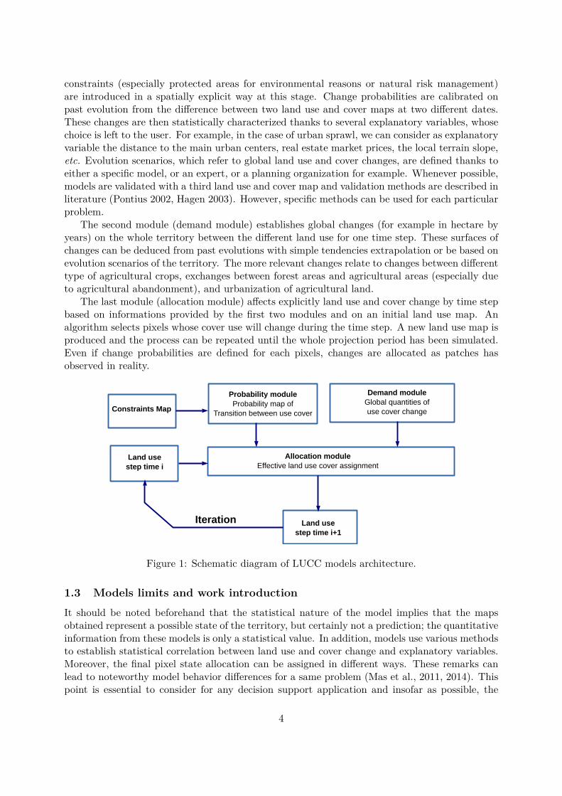
constraints (especially protected areas for environmental reasons or natural risk management)are introduced in a spatially explicit way at this stage. Change probabilities are calibrated onpast evolution from the difference between two land use and cover maps at two different dates.These changes are then statistically characterized thanks to several explanatory variables, whosechoice is left to the user. For example, in the case of urban sprawl, we can consider as explanatoryvariable the distance to the main urban centers, real estate market prices, the local terrain slope,etc. Evolution scenarios, which refer to global land use and cover changes, are defined thanks toeither a specific model, or an expert, or a planning organization for example. Whenever possible,models are validated with a third land use and cover map and validation methods are described inliterature (Pontius 2002, Hagen 2003). However, specific methods can be used for each particularproblem.

The second module (demand module) establishes global changes (for example in hectare byyears) on the whole territory between the different land use for one time step. These surfaces ofchanges can be deduced from past evolutions with simple tendencies extrapolation or be based onevolution scenarios of the territory. The more relevant changes relate to changes between differenttype of agricultural crops, exchanges between forest areas and agricultural areas (especially dueto agricultural abandonment), and urbanization of agricultural land.

The last module (allocation module) affects explicitly land use and cover change by time stepbased on informations provided by the first two modules and on an initial land use map. Analgorithm selects pixels whose cover use will change during the time step. A new land use map isproduced and the process can be repeated until the whole projection period has been simulated.Even if change probabilities are defined for each pixels, changes are allocated as patches hasobserved in reality.

Probability moduleProbability map of

Transition between use cover

Demand moduleGlobal quantities ofuse cover changeConstraints Map

Allocation moduleEffective land use cover assignment

Land usestep time i

Iteration Land usestep time i+1

Figure 1: Schematic diagram of LUCC models architecture.

1.3 Models limits and work introduction

It should be noted beforehand that the statistical nature of the model implies that the mapsobtained represent a possible state of the territory, but certainly not a prediction; the quantitativeinformation from these models is only a statistical value. In addition, models use various methodsto establish statistical correlation between land use and cover change and explanatory variables.Moreover, the final pixel state allocation can be assigned in different ways. These remarks canlead to noteworthy model behavior differences for a same problem (Mas et al., 2011, 2014). Thispoint is essential to consider for any decision support application and insofar as possible, the

4

modeler should evaluate the robustness of the conclusions for the decision-maker.Also, spatially explicit models are frequently cited and used in the literature but their descrip-

tion is incorrect. In particular, the theoretical background underlying such models is deficient,especially in comparison with the level of sophistication reached by the various modeling en-vironments mentioned above. Some modeling principles are used intuitively and pragmaticallywithout adequate justification; some of these are plainly wrong once formulated in an appropri-ate probability theory language. Indeed, no theoretical tools are available for neither softwareusers nor developers of other modeling environments even though those objects are essential toevaluate these models in a critical fashion. Important differences in performance can be noticedon specific problems but without any explication about the origin of quantitative discrepancies– even qualitative on occasion. These deficiencies impede systematic improvements of modelingperformances.

In this work which constitutes the first step in a more extensive LUCC theoretical analysis,we focused on a general approach. Introducing the notations used in this report, an explicittheoretical framework is introduced to define probabilities of change of land use/land cover. Thisframework is strictly correct only in the limiting case of statistically independent explanatoryvariables; this hypothesis is never satisfied in practice, but statistical correlations are minimized inpractice by an appropriate choice of these variables. In any case, it provides a useful framework toanalyze the origin of the problems of existing allocation procedures. I focused on what apparentlyconstitutes the most important limitation in LUCC modeling, i.e., the allocation procedure itself.A new conceptually correct allocation method is devised and presented. It is then applied in aactual problem. To this effect, I have developed a Python module called Demeter.

5

2 Notation and definitions

2.1 Pixel characterization parameters

We consider a study area for which we have raster data at a same scale for two or three differentdates. They are used for the calibration and the validation procedure of the land use and coverchange model.

Several quantities characterize a given pixel:

1. Each pixel is identified by its index j. J = [1, jm] is the set of all indexes.

2. Pixel coordinates are given by the couple (x, y). The coordinates of the pixel j are therefore(xj , yj). There is of course a bijection between the set J and the set of used coordinatecouples.

3. The symbol v refers to land use and cover types. A natural number is affected to each typeand therefore v ∈ [0, vm] where 0 refers to a lack of data and only [1, vm] are meaningful.We use also the term state to indicate a land use and cover type. The model calibrationis based on land use and cover at two different dates. vi and vf refers respectively to apixel state at the initial moment and the final one. For simplicity, these subscripts are alsointuitively used in the allocation phase: vi refers to the pixel state at the current step timeand vf is the allocation outcome state. Subsets of J can be defined regarding the land usestate. For example, Jvi = {j ∈ J, vj = vi}. In the following, the sequential aspect of landuse states is implicit, i.e. the subscript vi, vf refers to an element which have transitedfrom vi to vf during the studied phase. For example, Jvi,vf

is the set of pixel which havetransited from vi to vf .

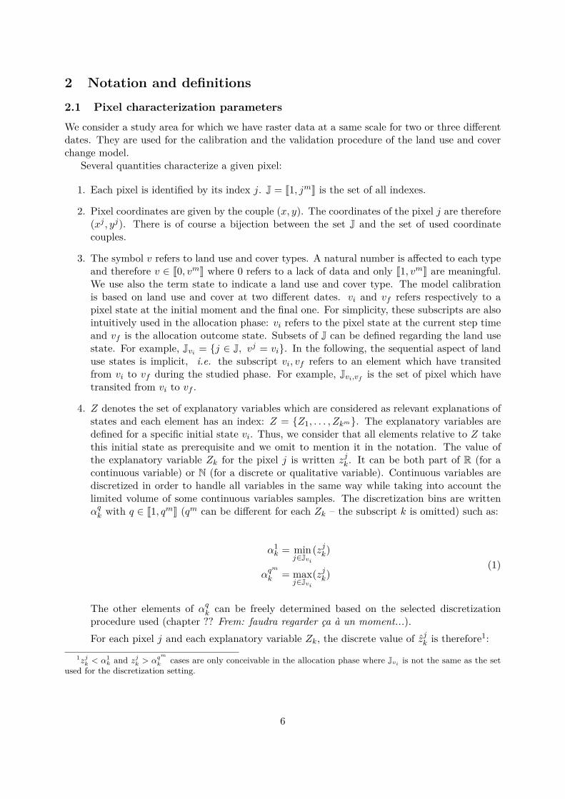
4. Z denotes the set of explanatory variables which are considered as relevant explanations ofstates and each element has an index: Z = {Z1, . . . , Zkm}. The explanatory variables aredefined for a specific initial state vi. Thus, we consider that all elements relative to Z takethis initial state as prerequisite and we omit to mention it in the notation. The value ofthe explanatory variable Zk for the pixel j is written zjk. It can be both part of R (for acontinuous variable) or N (for a discrete or qualitative variable). Continuous variables arediscretized in order to handle all variables in the same way while taking into account thelimited volume of some continuous variables samples. The discretization bins are writtenαqk with q ∈ [1, qm] (qm can be different for each Zk – the subscript k is omitted) such as:

α1k = min

j∈Jvi

(zjk)

αqm

k = maxj∈Jvi

(zjk)(1)

The other elements of αqk can be freely determined based on the selected discretizationprocedure used (chapter ?? Frem: faudra regarder ça à un moment...).For each pixel j and each explanatory variable Zk, the discrete value of zjk is therefore1:

1zjk < α1

k and zjk > αqm

k cases are only conceivable in the allocation phase where Jvi is not the same as the setused for the discretization setting.

6

zjk =

0 if zjk < α1

k

q | αqk ≤ zjk < αq+1

k if zjk < αqm

k

qm − 1 if zjk = αqm

k

qm if zjk > αqm

k

(2)

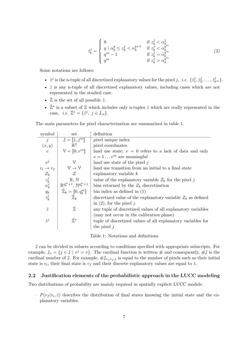
Some notations are follows:

• zj is the n-tuple of all discretized explanatory values for the pixel j, i.e. {zj1, zj2, . . . , z

jkm}.

• z is any n-tuple of all discretized explanatory values, including cases which are notrepresented in the studied case.

• Z is the set of all possible z.• Z∗ is a subset of Z which includes only n-tuples z which are really represented in the

case, i.e. Z∗ = {zj , j ∈ Jvi}.

The main parameters for pixel characterization are summarized in table 1.

symbol set definitionj J = [1, jm] pixel unique index

(x, y) R2 pixel coordinatesv V = [0, vm] land use state; v = 0 refers to a lack of data and only

v = 1 . . . vm are meaningfulvj V land use state of the pixel j

vi → vf V→ V land use transition from an initial to a final stateZk Z explanatory variable kzjk R, N value of the explanatory variable Zk for the pixel jαvk Rqm

k +1, Nqmk +1 bins returned by the Zk discretization

qk Zk = [0, qmk ] bin index as defined in (1)zjk Zk discretized value of the explanatory variable Zk as defined

in (2), for the pixel jz Z any tuple of discretized values of all explanatory variables

(may not occur in the calibration phase)zj Z∗ tuple of discretized values of all explanatory variables for

the pixel j

Table 1: Notations and definitions

J can be divided in subsets according to conditions specified with appropriate subscripts. Forexample, Jv = {j ∈ J | vj = v}. The cardinal function is written # and consequently, #J is thecardinal number of J. For example, #Jvi,vf ,z is equal to the number of pixels such as their initialstate is vi, their final state is vf and their discrete explanatory values are equal to z.

2.2 Justification elements of the probabilistic approach in the LUCC modeling

Two distributions of probability are mainly required in spatially explicit LUCC models:

– P (vf |vi, z) describes the distribution of final states knowing the initial state and the ex-planatory variables.

7

– P (z|vi, vf ) describes distribution of explanatory variables knowing initial and final states.

By drawing pixels, one get a simple but not exclusive way to introduce the probabilitiespresented above as random variables. As a draw defines simultaneously a value for all variables,on can define in this context the joint probability: P (Vi, Vf , Z) which defines the probability fora given pixel to transit from vi to vf during the time step. Also, for each step of the simulation,the final state is unknown and as for any problem with complex causes, one prefers handle theresult of the evolution as a random process product.

It is essential to understand the difference between the two probabilities introduced above.The first one is applied to any given pixel during the simulation. It gives the probability for thatpixel with the initial state vi and knowing its explanatory variables values to change to vf . Thesecond one corresponds to pixels repartitions function of explanatory variables knowing initial andfinal states. It cannot be the probability for a given pixel to present a specified z, because eachpixel has already a fixed z which does not change during the time step. During the calibrationstage, one can realize a fair sampling within the subset Jvi,vf

and get on average a distribution incompliance with P (z|vi, vf ). Thus, one use for the calibration the Bayes formula in the frequencysense. However, during a simulation, it is a priori a probability in the Bayesian sens whichdefines the distribution function of z, knowing vi and vf . To simulate a trend evolution based onthe calibration, the distribution is used as it is. Alternately, on can edit this probability duringthe simulation according to a specified scenario. This Bayesian aspect is used to relate the twoprobabilities in section 4.1. Also, only P (vf |vi, z) makes sense to generate a map of probabilityduring a simulation.

8

3 A case study: the SCoT of GrenobleThe ESNET project aims to analyse future land use trajectoires and their effects on biodiversityand ecosystem services for the Grenoble urban area. As part of this project, a case study dedicatedto LUCC had been defined and I use it as case study of this work.

The employment area of Grenoble covers 4 450 km2. In 2012 according to INSEE, theirwere 800 000 inhabitants and 500 000 jobs. The boundaries of this territory have been definedregarding the economic influence of the agglomeration of Grenoble and the diversity of landscapeswhich outline the region. The economic aspect, boundaries are based on EPCI2 areas. SelectedEPCIs belong to the SCoT3 of Grenoble and some surrounding EPCIs. On the landscape aspect,the region of Grenoble presents a large diversity of natural sites. Planar valleys of Grenobleand the Grésivaudan encourage urban extension. The three mountain ranges (the Vercors, theChartreuse and Belledone) structure the territory and provide natural landscape with numerousprotection areas (regional nature parks, nature reserve).

Thus, the employment area gather 311 municipalities in a radius of about fifty kilometersorganized in ten EPCIs: the agglomeration of Grenoble, the south of Grenoble, the Grésivaudanand around Voiron (these areas form the “Y” of Grenoble), the Chartreuse and the Vercors (whichare the mountain range areas apart from the SCoT of Grenoble), the Trièves, the Matheysine,the south of the Grésivaudan, the Bièvre Valloire (which are mainly agricultural plains).

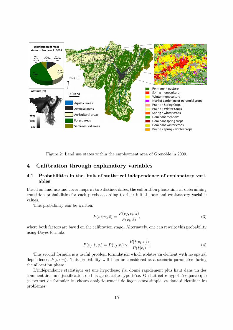
As part of the ESNET project, existing spatial data about this territory have been mergedwith photo interpretation and IGN maps in order to provide a data base of land use maps of1998, 2003 and 2009 with a precision of 15 meters (the pixel width). The topology of this database is composed by 34 states ranked in four precision levels (fig. 2). It distinguishes artificialareas (with within it residential zones, zones of industrial and commercial activity, roads, railwaynetworks. . . ). It describes also several agricultural types (with within it monocultures, pastures,market gardening. . . ). Forest and semi-natural4 environments are characterized at the populationlevel for wooded areas.

In this work, I focused on transitions from agriculture to urban residential area and zone ofindustrial and commercial activity. The land use maps used are then only constituted by 8 statesas described in table 2.

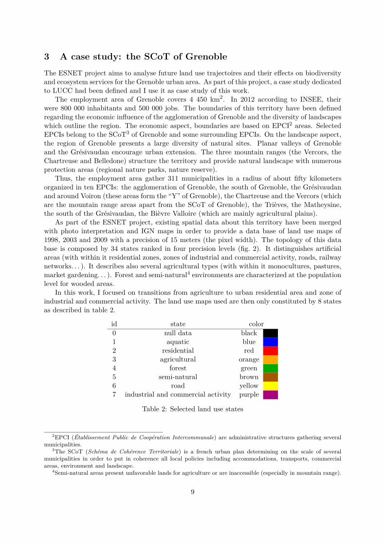
id state color0 null data black1 aquatic blue2 residential red3 agricultural orange4 forest green5 semi-natural brown6 road yellow7 industrial and commercial activity purple

Table 2: Selected land use states

2EPCI (Établissement Public de Coopération Intercommunale) are administrative structures gathering severalmunicipalities.

3The SCoT (Schéma de Cohérence Territoriale) is a french urban plan determining on the scale of severalmunicipalities in order to put in coherence all local policies including accommodations, transports, commercialareas, environment and landscape.

4Semi-natural areas present unfavorable lands for agriculture or are inaccessible (especially in mountain range).

9

Aquatic areas

Artificial areas

Agricultural areas

Forest areas

Semi-natural areas

NORTH

10 KM

2977

150

1000

Altitude (m)

Distribution of main states of land use in 2009

Legend

Successions_MODIS<all other values>

Code_MODIS0

1

2

4

6

7

8

9

10

11

12

13

14

15

16

17

18

19

Permanent pastureSpring monocultureWinter monocultureMarket gardening or perennial cropsPrairie / Spring CropsPrairie / Winter CropsSpring / winter cropsDominant meadowDominant spring cropsDominant winter cropsPrairie / spring / winter crops

Legend

Successions_MODIS<all other values>

Code_MODIS0

1

2

4

6

7

8

9

10

11

12

13

14

15

16

17

18

19

Legend

Successions_MODIS<all other values>

Code_MODIS0

1

2

4

6

7

8

9

10

11

12

13

14

15

16

17

18

19

Legend

Successions_MODIS<all other values>

Code_MODIS0

1

2

4

6

7

8

9

10

11

12

13

14

15

16

17

18

19

5 KM

Figure 2: Land use states within the employment area of Grenoble in 2009.

4 Calibration through explanatory variables

4.1 Probabilities in the limit of statistical independence of explanatory vari-ables

Based on land use and cover maps at two distinct dates, the calibration phase aims at determiningtransition probabilities for each pixels according to their initial state and explanatory variablevalues.

This probability can be written:

P (vf |vi, z) =P (vf , vi, z)P (vi, z)

, (3)

where both factors are based on the calibration stage. Alternately, one can rewrite this probabilityusing Bayes formula:

P (vf |z, vi) = P (vf |vi)×P (z|vi, vf )P (z|vi)

. (4)

This second formula is a useful problem formulation which isolates an element with no spatialdependence, P (vf |vi). This probability will then be considered as a scenario parameter duringthe allocation phase.

L’indépendance statistique est une hypothèse; j’ai donné rapidement plus haut dans un descommentaires une justification de l’usage de cette hypothèse. On fait cette hypothèse parce queça permet de formuler les choses analytiquement de façon assez simple, et donc d’identifier lesproblèmes.

10

To apply this Bayesian statistics approach and for simplicity, explanatory variables are con-sidered as independent random variables. This hypothesis is never satisfied but explanatoryvariables Z are chosen in order to approach it. It is often sufficient considering the precisionlevel aimed for LUCC modeling. It is possible to conceive more sophisticated statistic methodsfor calibration with dependent variables but keeping this hypothesis is very useful to pinpointthe various problems underlying incorrect (implicit or explicit) assumptions in existing modelingenvironments. With this assumption:

P (z|vi, vf ) =∏k

Pk(zk|vi, vf ) (5)

P (z|vi) =∏k

Pk(zk|vi) (6)

Where Pk only considers the explanatory variable Zk and the symbol P indicates that theindependent random variables hypothesis is used.

In practice, this hypothesis makes the transition probability easier to calibrate. Indeed, oneneeds a smaller amount of calibration data to calibrate a one variable probability at a givenprecision level, compared to multiple variable probabilities. In fact, the number of calibrationpixels is usually limited due to the relatively small number of pixels undergoing a transition of agiven type in the calibration data. Indeed, without equations (5 - 6), calibrating would mean toevaluate every distinct combinations of z. In the present case, it just implies to consider all binsof each explanatory variable separately. Also, this formulation allows to evaluate probabilitiesfor some (vi, z) combinations not occurring in the calibration data. Such combinations are notnecessarily unrealistic; they are only not represented due to the inherent sampling noise of thecalibration data.

Thereby:

P (vf |z, vi) = P (vf |vi)×∏k

Pk(zk|vi, vf )Pk(zk|vi)

(7)

Basically, probabilities are estimated by pixels counting:

P (vf |vi) =#Jvi,vf

#Jvi

(8)

Pk(zk|vi, vf ) =#Jvi,vf ,zk

#Jvi,vf

(9)

Pk(zk|vi, vf ) =#Jvi,zk

#Jvi

(10)

#Jx are random variables. As we got only one “statistical experience” which corresponds tothe observed reality, the noise question on probabilities estimation arises. Dinamica proposes acomputing method by weights of evidence described in section 4.2. Note that the calibration phasecould be here achieved and come down to know for all k Pk(zk|vi, vf ) and Pk(zk|vi). P (vf |vi) isdetermined by the scenario. Of course, the obtained probabilities verify the closure relations:

11

∑vf∈V

P (vf |vi) = 1 (11)

∑z∈Z

P (z|vi) =∑z∈Z

∏k

Pk(zk|vi) = 1 (12)

∀ vf ∈ V,∑z∈Z

P (z|vi, vf ) =∑z∈Z

∏k

Pk(zk|vi, vf ) = 1 (13)

∀ z ∈ Z∑vf∈V

P (vf |vi, z) = 1 (14)

4.2 Dinamica weights of evidence

The weights of evidence is a useful and generic method to characterize transition probabilitywhen explanatory variables are independent. However, the approximation used in Dinamica tocompute weights of evidence is particular and it proves to be constrained by a necessary condition.Dinamica makes this choice in order to reduce statistic noise due to the restricted sampling. Onepresents here only practical formulas.

Dinamica defines the weights of evidence W+k in the following way:

∀ zk, W+(zk|vi, vf ) = ln(Pk(zk|vi, vf )Pk(zk|vi)

)(15)

Thus:P (vf |vi, z) = P (vf |vi)

∏k

exp(W+(zk|vi, vf )) (16)

Dinamica only keeps track of the weights of evidence at the end of its calibration procedure.

4.3 Imperfect closure

Z∗ is a subset of all possible z which includes only z which are really represented in the calibrationcase. Then, we can write the inequation for all vf regarding the closure relations:∑

z∈Z∗P (z|vi, vf ) ≤

∑z∈Z

P (z|vi, vf ) = 1. (17)

In practice, it means that ∑z∈Z∗ P (z|vi, vf ) is lower than 1 because Z∗ is a subset of Z ,i.e. all z are not considered within the calibration phase. This also implies that for a given z,∑vf∈V P (vf |vi, z) is also lower than 1.Missing (vi, z) combinations in the calibration data are not the only reason of imperfect

closure. The lack of occurring cases is not the only origin of the closure relation rejection.Indeed, we have assumed the explanatory variables independence hypothesis. Yet, an error onthis assumption implies a wrong evaluation of P (z|vi, vf) and leads also to an error on the closurerelation.

12

5 Pruning and currently used allocation methodsWe present in this section the method used by Dinamica to perform the allocation phase. Thisdescription is required to propose then a new allocation method in section 6.

5.1 Position of the problem

In principle, and without making any specific assumption, the allocation process can be viewedas a two-step process at any time step p in a simulation. First one randomly selects a pixel in J.This random selection results in a known vjp, zj for the selected pixel. Second, one allocates tothis pixel a final state, vjp+1.

This being said, without further relying on some form of a priori knowledge, this procedure,although theoretically correct, is extremely inefficient; inefficient here means that most randomdraws of pixels are performed uselessly as most pixels will not change state, so that most of thecomputational time will be spent in checking that no transition occurs. All software suffer fromthis problem; in order to minimize it, a preselection stage, called pruning, is introduced and twodifferent modes of pruning are used in Dinamica and LCM.

We can now now specify the various stages of the allocation procedure that should actuallybe implemented for efficiency purposes:

1. Pruning (preselection) of an ensemble of appropriate pixels for transitions from vjp to otherstates vjp+1.

2. Random selection of a pixel in this pruned ensemble.

3. Allocation of a final state to this pixel.

This being said, it is unclear which procedure to choose in the pruning and allocation steps,the only clear step being the random selection of a pixel once pruning is done. The present sectionis devoted to clarifying this issue. First, the procedures used in LCM and Dinamica are recalled.Then, the conceptually correct procedure is constructed. This will show that neither Dinamicanor LCM are correct in their choices.

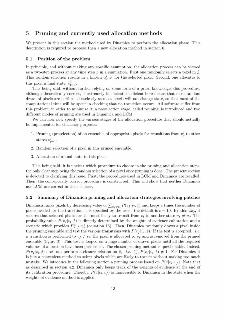
5.2 Summary of Dinamica pruning and allocation strategies involving patches

Dinamica ranks pixels by decreasing value of ∑vf 6=viP (vf |vi, z) and keeps c times the number of

pixels needed for the transition. c is specified by the user ; the default is c = 10. By this way, itassures that selected pixels are the most likely to transit from vi to another state vf 6= vi. Theprobability value P (vf |vi, z) is directly determined by the weights of evidence calibration and ascenario which provides P (vf |vi) (equation 16). Then, Dinamica randomly draws a pixel insidethe pruning ensemble and test the various transitions with P (vf |vi, z). If the test is accepted, i.e.a transition is performed to vf 6= vi, the pixel is allocated to vf and is removed from the prunedensemble (figure 3). This test is looped on a huge number of drawn pixels until all the requiredvolumes of allocation have been performed. The chosen pruning method is questionable. Indeed,P (vf |vi, z) does not perform a closure relation on z, i.e.

∑z P (vf |vi, z) 6= 1. For Dinamica it

is just a convenient method to select pixels which are likely to transit without making too muchmistake. We introduce in the following section a pruning process based on P (z|vi, vf ). Note thatas described in section 4.2, Dinamica only keeps track of the weights of evidence at the end ofits calibration procedure. Thereby, P (z|vi, vf ) is inaccessible to Dinamica in the state when theweights of evidence method is applied.

13

vi pixels pruningallocation

objective achieved?

pixel random draw

Acceptation testP (vf |vi, z)

Patch allocationarround the kernel pixel

For all transition

pixelsno

rejeté

accepted

allocated pixelsare removed fromthe pruning set

yes

sequential

data

Figure 3: Schematic Dinamica allocation procedure.

The tension between the basic units of map characterization – pixels – and the basic units ofLUCC change – patches according ecological observations, i.e. connected (often simply connectedin the mathematical sense) ensembles of pixels – is ubiquitous in LUCC modeling, but does notseem to have been discussed or resolved in the literature.

All LUCC models only employ distribution functions for a single pixel. For example, anexplanatory variable such as the distance to road describes the probability for a drawn pixel tobe at a given distance from the road. Yet, a patch is defined as a manifestation of a correlationbetween of adjacent pixels. It implies that the probability that a pixel changes state is muchgreater if a nearby pixel also changes state. State changes are not independent between nearbypixels and probabilities for several pixels are not simply the product of single pixel probabilities.

In these conditions, the single pixel function (the usual probability in models) does not containthe whole information required to model cover change and it would make more sense to developn-pixels probabilities. Distribution functions implying several objects are problematic becauseit is in practice very difficult to obtain a reliable theory when the correlations between objectsare strong and the number of objects involved is large, which is precisely the case with patches.This complex approach is then not possible here and it is simpler to directly compute probabilitydistribution of patches.

Even though one can imagine ecological processes that would occur at singular points moreor less randomly distributed in space, most if not all LUCC models tackle LUCC changes thatare known to occur in patches, i.e., across many connected pixels at once, and usually for quitea few such patches per unit time step. As single pixel probabilities are easy to manage, thecommunity has developed these methods without considering formal relations between singlepixel probabilities and probability distribution of patches. Pixels drawn by Dinamica by singlepixel probabilities are therefore considered as kernel pixels and a patch builder called to allocateempirically pixels around the kernel pixel according to patch parameters defined by the user. Itshould be noted that this is the most sophisticated approach used in the literature and in practiceto date.

Their is definitely a relation between kernel pixel probabilities and single pixel probabilities.

14

Under certain conditions which are probably often satisfied in practice, the both probabilitydistributions are virtually identical. This aspect is not addressed at all in the literature butPierre-Yves Longaretti has studied it and has identified conditions of validity testable on data.His work is not yet published and it will be reviewed and enriched during the course of the PhD.

5.3 Defining conceptually correct pruning

Because the explanatory variables Z are initially chosen in terms of their relevance for the tran-sitions to be allocated, one expects that the higher P (z|vi, vf ) for any pixel, the higher thecontribution of such pixels to the overall transition. This intuitive argument suggests that this isthe correct quantity to be used for pruning, a point that we justify here in a more formal way.

Recall firsts the point made above that for the transition vi → vf , the first pruning selectioncriterion is obvious: one keeps only pixels belonging to Jvi as vi must be a conditionally knownquantity in the process.

To proceed further, note that

#Jvi,vf= P (vi|vf )#Jvi =

∑z

P (z, vf |vi)#Jvi (18)

is the total number of pixels changing state from vi to vf . Therefore, the higher P (z, vf |vi), themost likely the corresponding pixels (Jvi,vf ,z), whose number amounts to #Jvi,vf ,z = P (z, vf |vi)#Jvi ,are to contribute to Jvi,vf

. Conversely, one cannot rely on P (vf |z, vi) to identify the most likelypixels to undergo the required transition, as there is no closure relation on z on this probabil-ity, i.e.

∑z P (vp+1|z, vp) 6= 1; this simple remark disqualifies the choice made in Dinamica. In

fact, the probability distribution P (z, vf |vi) is clearly the only one having P (vf |vi) as marginalprobability at given starting state, so that the point made in this paragraph is unavoidable.

Note that one can equivalently use P (z|vi, vf ) = P (z, vf |vi)/P (vf |vi) to define a pruningensemble for the vi → vf transition, because P (vf |vi) is pixel independent; algebraically, thisfollows because one can also write #Jvf ,vi,z = P (z|vf , vi)#Jvi,vf

, so that the higher P (z|vf , vi),the most likely the corresponding pixels (Jvi,vf ,z) will contribute to Jvi,vf

.An extreme case of this argument occurs when a vast majority of pixels j have zero contribu-

tion to the sum, i.e., P (z, vp+1|vp) = 0. Removing these pixels from Jvp does not change anythingin the final allocation, but considerably reduces the required number of random pixel selection.By extension, removing the pixels with small probability P (z|vi, vf ) should have little effect onthe result.

At first sight, it might be surprising that the pruning criterion involves a probability distri-bution P (z|vi, vf ) that differs from the allocation procedure one P (vf |z, vi). On second thought,this is quite normal: the pruning criterion occurs prior to randomly selecting a pixel, i.e. beforez is known, while the allocation procedure occurs after random selection, i.e. after z is known.Pruning and allocation are therefore two essentially different processes, and there is no reasonthey should be based on the same conditional probability.

Let us now turn to the actual elaboration of a pruning procedure. Consider first the case witha single transition vi → vf . According to the preceding argument, it is logical to order the pixelsin decreasing values of P (z|vi, vf ).

For any given τ ∈ [0, 1], one can define a subset of Z:

Zτ = {z ∈ Z |∑z∈Z

P (z|vi, vf ) ≥ τ} (19)

15

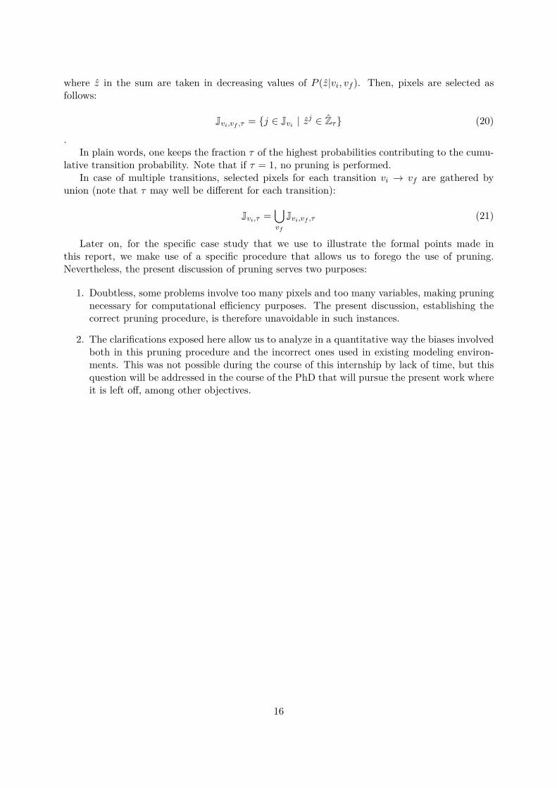
where z in the sum are taken in decreasing values of P (z|vi, vf ). Then, pixels are selected asfollows:

Jvi,vf ,τ = {j ∈ Jvi | zj ∈ Zτ} (20)

.In plain words, one keeps the fraction τ of the highest probabilities contributing to the cumu-

lative transition probability. Note that if τ = 1, no pruning is performed.In case of multiple transitions, selected pixels for each transition vi → vf are gathered by

union (note that τ may well be different for each transition):

Jvi,τ =⋃vf

Jvi,vf ,τ (21)

Later on, for the specific case study that we use to illustrate the formal points made inthis report, we make use of a specific procedure that allows us to forego the use of pruning.Nevertheless, the present discussion of pruning serves two purposes:

1. Doubtless, some problems involve too many pixels and too many variables, making pruningnecessary for computational efficiency purposes. The present discussion, establishing thecorrect pruning procedure, is therefore unavoidable in such instances.

2. The clarifications exposed here allow us to analyze in a quantitative way the biases involvedboth in this pruning procedure and the incorrect ones used in existing modeling environ-ments. This was not possible during the course of this internship by lack of time, but thisquestion will be addressed in the course of the PhD that will pursue the present work whereit is left off, among other objectives.

16

6 New land use change allocation algorithmDinamica allocation principle is based on a pruning selection. Indeed, this software spends alarge part of the computation time to pick and reject pixels. It seems that bad developmentchoices are behind this wasting operation. In order to conceive a new allocation algorithm whichcould be fast and theoretically correct, we developed a new allocation procedure called Deme-ter5 written in Python 3. This allocation procedure will eventually turn into a new full LUCCmodeling environment during the course of the PhD that will be devoted to the problem. Thislanguage choice, different from Dinamica which is written in C++, has several advantages. First,Python is an interpreted, high-level, general-purpose programming language which has a highcode readability and provides a large amount of efficient libraries. Three libraries are especiallyemployed in Demeter: Numpy for large matrix manipulations, Scipy for digital image processing( i.e. map processing) and Pandas for database manipulation. These libraries enable the designof a high efficient LUCC model. Second, the desktop graphic information system QGIS6 providesa very simple python plug-in implementation. That way, it is straightforward to design a GUIlayer over our python model to call it and visualize directly the results on QGIS.

This new allocation algorithm is based on a very efficient generalized acceptation rejectiontest which is able to evaluate transition of a large number of pixels for all possible transitions asdescribed in section 6.2.

6.1 Calibration and allocation scenario

The calibration phase provided for all pixel j probabilities for transition from vi to any other vfaccording to the Bayes formula (eq. 4 reminded below).

P (vf |z, vi) = P (vf |vi)×P (z|vi, vf )P (z|vi)

(4 revisited)

P (z|vi, vf ) and P (z|vi) are both coming from the calibration. Using the explanatory variableindependence hypothesis allows us to deal with combinations of explanatory variable values thatare not present in the calibration data. P (vf |vi) is considered as a scenario parameter andis defined by the user. This probability is directly related to the targeted transited surface#Jvi,vf

= #JviP (vf |vi).

6.2 Generalized acceptation rejection test

An essential step of the allocation process concerns the transition test from vi to vf . In orderto insure a statistically correct draw, it is necessary to test all possible transitions at the sametime. Von Neumann (1951) presents a method to test a simple acceptation function. A multipleacceptation rejection test is proposed by Sunter (1977) without replacement in the sample. Wedefine therefore a simpler method of generalized acceptation rejection test (GART) which is usedto determine a potential land use change for a given pixel. The simplification is that the drawprobabilities are not updated to reflect the fact that the overall sample is decreasing. One justifiesby the fact that the sample is very large in front of the number of pixels drawn.

5In ancient Greek mythology, Demeter is the goddess of the harvest and agriculture, presiding over grains andthe fertility of the earth.

6QGIS is a free and open-source cross-platform desktop geographic information system (GIS) application thatsupports viewing, editing, and analysis of geospatial data.

17

For a pixel j, knowing vji and zj , the calibration allows to determine P (vf |vji , zj) for all vf(eq. 4). For this purpose, we define ηp, ∀[0, vm] as the cumulative sum of P (vf |vji , zj):

η0 = 0

∀p ∈ [1, vm], ηp =p∑

vf =1P (vf |vi, z)

(22)

Then, a simple random float is sufficient to test simultaneously all possible transitions for j.For x, a random float in the half-open interval [0, 1), it exists ηp such as ηp−1 ≤ x < ηp. The testreturns in that case p.

We define ϕ as the random function of the generalized acceptation rejection test which takesthe pixel j and returns a state p ∈ V as a random variable. If p 6= vji , the test is said as acceptedand as rejected otherwise.

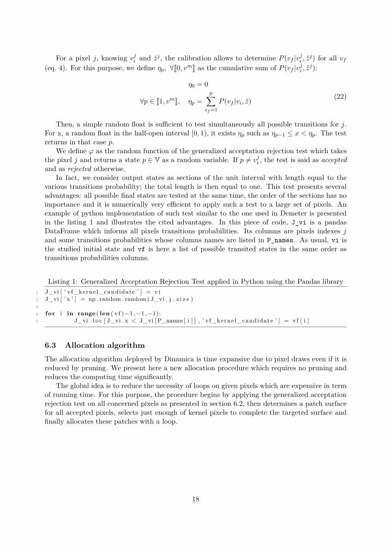
In fact, we consider output states as sections of the unit interval with length equal to thevarious transitions probability; the total length is then equal to one. This test presents severaladvantages: all possible final states are tested at the same time, the order of the sections has noimportance and it is numerically very efficient to apply such a test to a large set of pixels. Anexample of python implementation of such test similar to the one used in Demeter is presentedin the listing 1 and illustrates the cited advantages. In this piece of code, J_vi is a pandasDataFrame which informs all pixels transitions probabilities. Its columns are pixels indexes jand some transitions probabilities whose columns names are listed in P_names. As usual, vi isthe studied initial state and vf is here a list of possible transited states in the same order astransitions probabilities columns.

Listing 1: Generalized Acceptation Rejection Test applied in Python using the Pandas library1 J_vi [ ’ v f_kernel_candidate ’ ] = v i2 J_vi [ ’ x ’ ] = np . random . random( J_vi . j . s i z e )3

4 for i in range ( len ( v f )−1 ,−1 ,−1):5 J_vi . l o c [ J_vi . x < J_vi [ P_names [ i ] ] , ’ v f_kernel_candidate ’ ] = vf [ i ]

6.3 Allocation algorithm

The allocation algorithm deployed by Dinamica is time expansive due to pixel draws even if it isreduced by pruning. We present here a new allocation procedure which requires no pruning andreduces the computing time significantly.

The global idea is to reduce the necessity of loops on given pixels which are expensive in termof running time. For this purpose, the procedure begins by applying the generalized acceptationrejection test on all concerned pixels as presented in section 6.2, then determines a patch surfacefor all accepted pixels, selects just enough of kernel pixels to complete the targeted surface andfinally allocates these patches with a loop.

18

GARTa appliedto all pixels

While the allocationobjective is not achieved

random drawof patch surfaces

random drawof required kernel pixelsto achieved the objective

Patch allocation

If the objective is unfiledand potential surface

is sufficient

kernel pixelskernel pixels withassigned surface

remove allo-cated pixels

selected kernel pixelswith assigned surface

truefalse

sequential

données(a) Generalized Acceptation Rejection Test

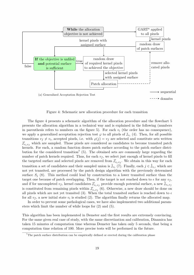
Figure 4: Schematic new allocation procedure for each transition

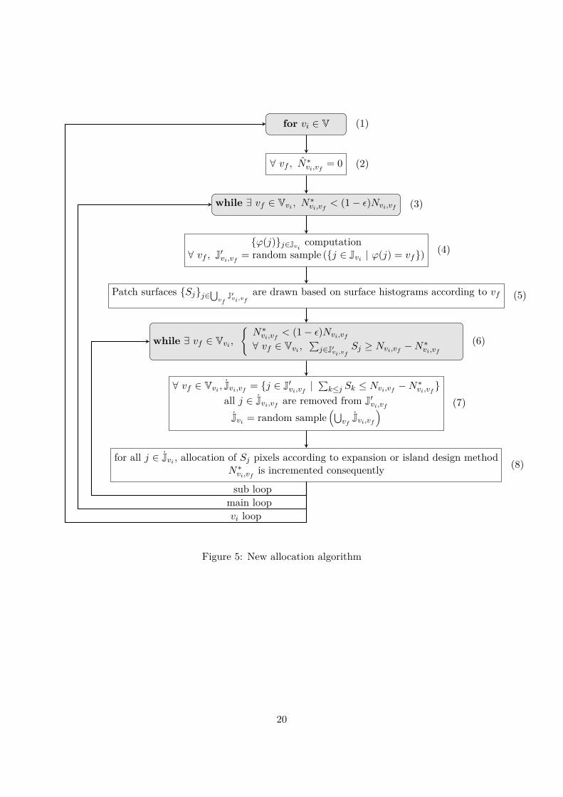
The figure 4 presents a schematic algorithm of the allocation procedure and the flowchart 5presents the allocation algorithm in a technical way and is explained in the following (numbersin parenthesis refers to numbers on the figure 5). For each vi (the order has no consequence),we apply a generalized acceptation rejection test ϕ to all pixels of Jvi (4). Then, for all possibletransitions vf 6= vi, accepted pixels, i.e. with ϕ(j) = vf are selected and constitute sets writtenJ′vi,vf

which are sampled. Those pixels are considered as candidates to become transited patchkernels. For each, a random function draws patch surface according to the patch surface distri-bution for the considered transition7 (5). The obtained sets are commonly large regarding thenumber of patch kernels required. Thus, for each vf , we select just enough of kernel pixels to fillthe targeted surface and selected pixels are removed from J′vi,vf

. We obtain in this way for eachtransition a set of candidates and their sampled union is Jvi (7). Finally, each j ∈ Jvi , which arenot yet transited, are processed by the patch design algorithm with the previously determinedsurface Sj (8). This method could lead by construction to a lower transited surface than thetarget one because of patch overlapping. Then, if the target is not reached down to ε for any vf ,and if for uncompleted vf , kernel candidates J′vi,vf

provide enough potential surface, a new Jvi,vf

is constituted from remaining pixels within J′vi,vf(6). Otherwise, a new draw should be done on

all pixels which are not yet transited (3). When the total transited surface is reached down to εfor all vf , a new initial state vi is studied (2). The algorithm finally returns the allocated map.

In order to prevent some pathological cases, we have also implemented two additional param-eters which limit the number of while loops for (2) and (5).

This algorithm has been implemented in Demeter and the first results are extremely convincing.For the same given real case of study, with the same discretization and calibration, Dinamica hastaken 15 minutes of computation time whereas Demeter has taken only 5 seconds, that being acomputation time relation of 100. More precise tests will be performed in the future.

7The patch surface distribution can be empirically defined or erected during the calibration phase

19

for vi ∈ V (1)

∀ vf , N∗vi,vf= 0 (2)

while ∃ vf ∈ Vvi , N∗vi,vf

< (1− ε)Nvi,vf (3)

{ϕ(j)}j∈Jvicomputation

∀ vf , J′vi,vf= random sample ({j ∈ Jvi | ϕ(j) = vf}) (4)

Patch surfaces {Sj}j∈⋃vf

J′vi,vfare drawn based on surface histograms according to vf (5)

while ∃ vf ∈ Vvi ,

{N∗vi,vf

< (1− ε)Nvi,vf

∀ vf ∈ Vvi ,∑j∈J′vi,vf

Sj ≥ Nvi,vf−N∗vi,vf

(6)

∀ vf ∈ Vvi , Jvi,vf= {j ∈ J′vi,vf

|∑k≤j Sk ≤ Nvi,vf

−N∗vi,vf}

all j ∈ Jvi,vfare removed from J′vi,vf

Jvi = random sample(⋃

vfJvi,vf

) (7)

for all j ∈ Jvi , allocation of Sj pixels according to expansion or island design methodN∗vi,vf

is incremented consequently (8)

sub loopmain loopvi loop

Figure 5: New allocation algorithm

20

7 Islands and expansions allocation proceduresThe actual allocation procedure has no vocation to be a prediction. It should only present aplausible final situation which corresponds to the requested scenario. Two patches types can bedistinguished: expansions and islands. The first one refers to transitions which occur on theboundary between vi and vf . The second one is about transitions which come out in vi withoutany vf adjacency.

In principle, their is no reason to make this distinction – it occurs inherently due to thedistribution of patch sizes and statistic choices of kernel pixel positions. In practice, distinguishexpansion and island patches is useful for two reasons: certain transitions present actually differentcharacteristics in both cases and it could also be numerically easier to use specific algorithm forboth cases.

7.1 Calibration

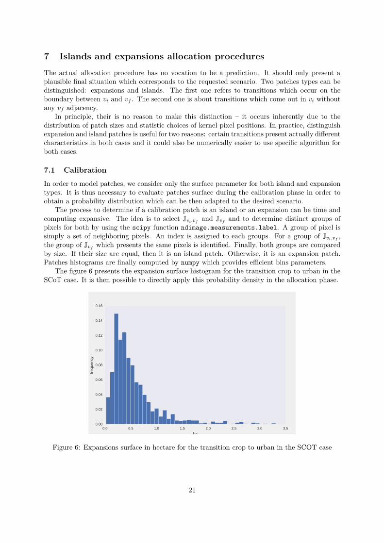
In order to model patches, we consider only the surface parameter for both island and expansiontypes. It is thus necessary to evaluate patches surface during the calibration phase in order toobtain a probability distribution which can be then adapted to the desired scenario.

The process to determine if a calibration patch is an island or an expansion can be time andcomputing expansive. The idea is to select Jvi,vf

and Jvfand to determine distinct groups of

pixels for both by using the scipy function ndimage.measurements.label. A group of pixel issimply a set of neighboring pixels. An index is assigned to each groups. For a group of Jvi,vf

,the group of Jvf

which presents the same pixels is identified. Finally, both groups are comparedby size. If their size are equal, then it is an island patch. Otherwise, it is an expansion patch.Patches histograms are finally computed by numpy which provides efficient bins parameters.

The figure 6 presents the expansion surface histogram for the transition crop to urban in theSCoT case. It is then possible to directly apply this probability density in the allocation phase.

0.0 0.5 1.0 1.5 2.0 2.5 3.0 3.5ha

0.00

0.02

0.04

0.06

0.08

0.10

0.12

0.14

0.16

freq

uenc

y

Figure 6: Expansions surface in hectare for the transition crop to urban in the SCOT case

21

7.2 Island design process

In order to design a patch, all methods begin from a first pixel called kernel pixel. Then, severalpossibilities can be considered to create an island patch associated to this kernel pixel:

– Dinamica uses a recursive algorithm based on a anisotropic parameter.

– It is possible to sample the required shape from a bank of shapes, itself constructed from thecalibration data. Then, a geometric similarity is randomly applied (size and orientation) tocorrespond to the desired surface.

– It is also possible to use a simple elliptic function or any other shape with the desiredsurface. This option however will tend to produce figures that are too regular compared toreality.

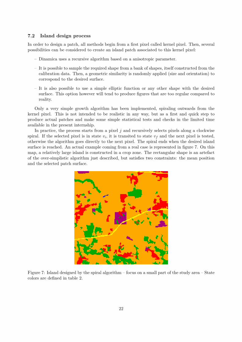
Only a very simple growth algorithm has been implemented, spiraling outwards from thekernel pixel. This is not intended to be realistic in any way, but as a first and quick step toproduce actual patches and make some simple statistical tests and checks in the limited timeavailable in the present internship.

In practice, the process starts from a pixel j and recursively selects pixels along a clockwisespiral. If the selected pixel is in state vi, it is transited to state vf and the next pixel is tested,otherwise the algorithm goes directly to the next pixel. The spiral ends when the desired islandsurface is reached. An actual example coming from a real case is represented in figure 7. On thismap, a relatively large island is constructed in a crop zone. The rectangular shape is an artefactof the over-simplistic algorithm just described, but satisfies two constraints: the mean positionand the selected patch surface.

Figure 7: Island designed by the spiral algorithm – focus on a small part of the study area – Statecolors are defined in table 2.

22

7.3 Expansion design process

The expansion process implies to evaluate the transition probability on the border of alreadypresent vf pixels. Soares-Filho et al. (2002) propose a method which favors pixels with higherP (vf |vi, z) and higher number of vf neighbors. I propose here a method based on matrix oper-ations in order to reduce computing time cost. In order to select border pixels, we perform thefollowing convolution:

M∗vf= Mvf

∗

0 1 01 0 10 1 0

(23)

where Mvfis a zero matrix of dimension equal to the map whose values of coordinates of pixels

belonging to Jvfare 1. M∗vf

is then a matrix which indicates for each pixel the number of vfneighbors. It is then easy to select pixels from Jvi with at least one neighbor in the desiredpost-transition state. We can then evaluate transition probability for these border pixels.

The expansion process idea is based on the evaluation of the transition probabilities aroundalready transited pixels. However, a simple algorithm which takes the highest probability aroundpixels of the desired state can lead to create biased expansion patches, again because correlationsbetween pixels are ignored in such a procedure. A simple way to create more satisfying patchesis to draw the new pixel in the list of neighbors with probabilities weights scaled to one. It ispresented in the algorithm 1 which does not verify if a pixel is already in the pixel neighbors list.This fact gives more weight to pixels with several neighbors already transited.

Algorithm 1: New allocation procedureData: vi, vf , the kernel pixel j and the desired surface SResult: Jvi,vf

S∗ = 0add all neighbors of j which are vi in Jj∗while S∗ < S and #Jj∗ > 0 doP is the set of ordered transition probabilities of Jj∗a pixel to transite is drawn in Jj∗ with P as weightsS∗ is incremented by oneall neighbors of the new transited pixel, which are vi, are appended to Jj∗

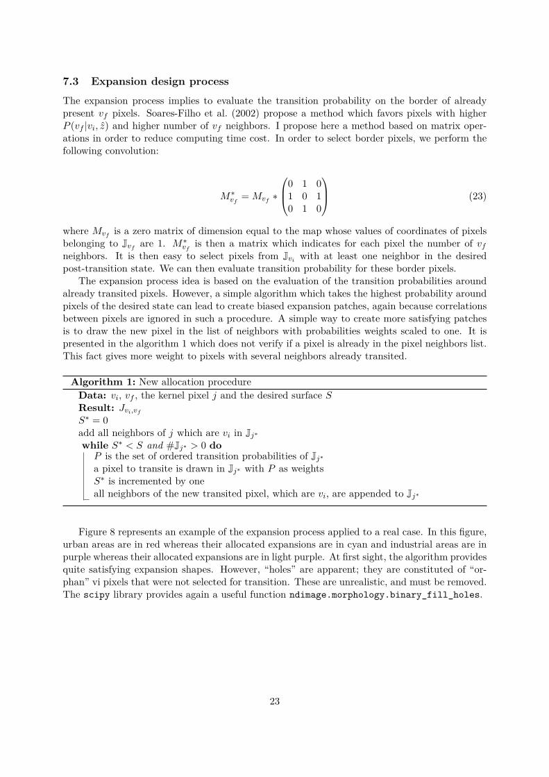
Figure 8 represents an example of the expansion process applied to a real case. In this figure,urban areas are in red whereas their allocated expansions are in cyan and industrial areas are inpurple whereas their allocated expansions are in light purple. At first sight, the algorithm providesquite satisfying expansion shapes. However, “holes” are apparent; they are constituted of “or-phan” vi pixels that were not selected for transition. These are unrealistic, and must be removed.The scipy library provides again a useful function ndimage.morphology.binary_fill_holes.

23

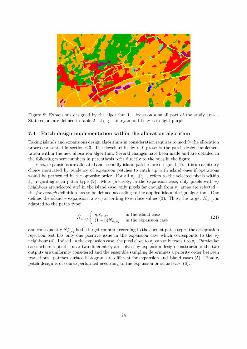
Figure 8: Expansions designed by the algorithm 1 – focus on a small part of the study area –State colors are defined in table 2 – J3→2 is in cyan and J3→7 is in light purple.

7.4 Patch design implementation within the allocation algorithm

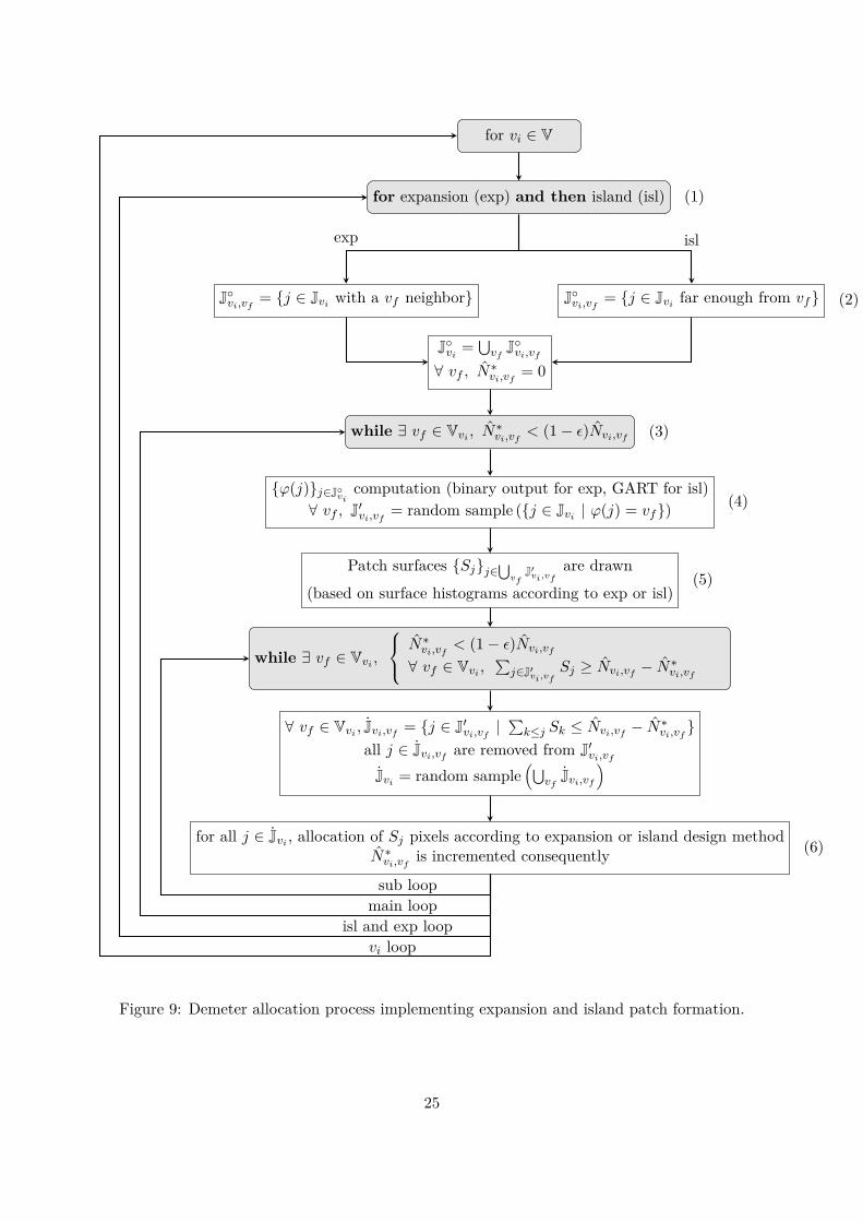
Taking islands and expansions design algorithms in consideration requires to modify the allocationprocess presented in section 6.3. The flowchart in figure 9 presents the patch design implemen-tation within the new allocation algorithm. Several changes have been made and are detailed inthe following where numbers in parenthesis refer directly to the ones in the figure.

First, expansions are allocated and secondly island patches are designed (1). It is an arbitrarychoice motivated by tendency of expansion patches to catch up with island ones if operationswould be performed in the opposite order. For all vf , J◦vi,vf

refers to the selected pixels withinJvi regarding such patch type (2). More precisely, in the expansion case, only pixels with vfneighbors are selected and in the island case, only pixels far enough from vf areas are selected –the far enough definition has to be defined according to the applied island design algorithm. Onedefines the island – expansion ratio η according to surface values (3). Thus, the target Nvi,vf

isadapted to the patch type:

Nvi,vf

{ηNvi,vf

in the island case(1− η)Nvi,vf

in the expansion case (24)

and consequently N∗vi,vfis the target counter according to the current patch type. the acceptation

rejection test has only one positive issue in the expansion case which corresponds to the vfneighbour (4). Indeed, in the expansion case, the pixel close to vf can only transit to vf . Particularcases where a pixel is near two different vf are solved by expansion design construction: the twooutputs are uniformly considered and the ensemble sampling determines a priority order betweentransitions. patches surface histogram are different for expansion and island cases (5). Finally,patch design is of course performed according to the expansion or island case (6).

24

for vi ∈ V

for expansion (exp) and then island (isl) (1)

J◦vi,vf= {j ∈ Jvi with a vf neighbor} J◦vi,vf

= {j ∈ Jvi far enough from vf} (2)

J◦vi= ⋃

vfJ◦vi,vf

∀ vf , N∗vi,vf= 0

while ∃ vf ∈ Vvi , N∗vi,vf

< (1− ε)Nvi,vf (3)

{ϕ(j)}j∈J◦vicomputation (binary output for exp, GART for isl)

∀ vf , J′vi,vf= random sample ({j ∈ Jvi | ϕ(j) = vf})

(4)

Patch surfaces {Sj}j∈⋃vf

J′vi,vfare drawn

(based on surface histograms according to exp or isl)(5)

while ∃ vf ∈ Vvi ,

N∗vi,vf< (1− ε)Nvi,vf

∀ vf ∈ Vvi ,∑j∈J′vi,vf

Sj ≥ Nvi,vf− N∗vi,vf

∀ vf ∈ Vvi , Jvi,vf= {j ∈ J′vi,vf

|∑k≤j Sk ≤ Nvi,vf

− N∗vi,vf}

all j ∈ Jvi,vfare removed from J′vi,vf

Jvi = random sample(⋃

vfJvi,vf

)

for all j ∈ Jvi , allocation of Sj pixels according to expansion or island design methodN∗vi,vf

is incremented consequently (6)

exp isl

sub loopmain loop

isl and exp loopvi loop

Figure 9: Demeter allocation process implementing expansion and island patch formation.

25

8 ConclusionThis preliminary work of the PhD has introduced several aspects of LUCC models which requiremore detailed studies. It takes part in the progression toward a general theoretical framework.Some bias implied by the supposed independence of explanatory variables has been describedand should be the main topic of a future work by defining a threshold condition of independence.Likewise, the patch point of view for LUCC has been presented and conditions to use single pixelprobabilities to draw kernel pixels deserve a specific attention in the future. I focused on theallocation procedure by analysing Dinamica choices, especially about the pruning method whichis proving to use a wrong statistical value (P (vf |vi, z) instead of P (z|vi, vf )). A correct pruningmethod is then defined. I introduce a new allocation method which apply simultaneously theacceptation rejection test to all pixels. It is then convenient to draw kernel pixels within theaccepted population. This procedure avoid the pitfall of Dinamica which draws a large amount ofpixels which are then rejected. This new algorithm already shows off very promising results witha saving of time of calculation of factor 100. More precise tests will be performed in the future.Finally, numerical considerations have been advanced about the practical allocation operation forboth patch types that are island and expansion.

Future work are already envisaged. First on the allocation procedure, allocation patch design,performance comparison with other softwares and pruning error evaluation have to be studied.Also the theory of patch modeling have to be explored as well as markovian aspect of LUCCmodels.

26

ReferencesChetan Agarwal, Glen M. Green, J. Morgan Grove, Tom P. Evans, and Charles M. Schweik. Areview and assessment of land-use change models: Dynamics of space, time, and human choice.Technical Report NE-GTR-297, U.S. Department of Agriculture, Forest Service, NortheasternResearch Station, Newtown Square, PA, 2002. 1.1

J. Ronald Eastman. IDRISI Selva Manual, Guide to GIS and Image Processing. Clark University,2012. 1.1

Alex Hagen. Fuzzy set approach to assessing similarity of categorical maps. International Journalof Geographical Information Science, 17(3):235–249, April 2003. ISSN 1365-8816, 1362-3087.doi: 10.1080/13658810210157822. 1.2

Jean-François Mas, Melanie Kolb, Thomas Houet, Martin Paegelow, and Maria Camacho Olmedo.Éclairer le choix des outils de simulation des changements des modes d’occupation et d’usagesdes sols. Une approche comparative. page 27, 2011. 1.3

Jean-François Mas, Melanie Kolb, Martin Paegelow, María Teresa Camacho Olmedo, and ThomasHouet. Inductive pattern-based land use/cover change models: A comparison of four softwarepackages. Environmental Modelling & Software, 51:94–111, January 2014. ISSN 13648152. doi:10.1016/j.envsoft.2013.09.010. 1.3

R Gil Pontius. Statistical Methods to Partition Effects of Quantity and Location During Compar-ison of Categorical Maps at Multiple Resolutions. PHOTOGRAMMETRIC ENGINEERING,page 9, 2002. 1.2

Britaldo Silveira Soares-Filho, Gustavo Coutinho Cerqueira, and Cássio Lopes Pennachin. Di-namica—a stochastic cellular automata model designed to simulate the landscape dynamicsin an Amazonian colonization frontier. Ecological Modelling, 154(3):217–235, September 2002.ISSN 03043800. doi: 10.1016/S0304-3800(02)00059-5. 1.1, 7.3

A. B. Sunter. List Sequential Sampling with Equal or Unequal Probabilities without Replacement.Applied Statistics, 26(3):261, 1977. ISSN 00359254. doi: 10.2307/2346966. 6.2

Peter H. Verburg and Koen P. Overmars. Combining top-down and bottom-up dynamics in landuse modeling: Exploring the future of abandoned farmlands in Europe with the Dyna-CLUEmodel. Landscape Ecology, 24(9):1167–1181, November 2009. ISSN 0921-2973, 1572-9761. doi:10.1007/s10980-009-9355-7. 1.1

Peter H. Verburg, Welmoed Soepboer, A. Veldkamp, Ramil Limpiada, Victoria Espaldon, andSharifah S.A. Mastura. Modeling the Spatial Dynamics of Regional Land Use: The CLUE-SModel. Environmental Management, 30(3):391–405, September 2002. ISSN 0364-152X, 1432-1009. doi: 10.1007/s00267-002-2630-x. 1.1

Peter H. Verburg, Kasper Kok, Robert Gilmore Pontius, and A. Veldkamp. Modeling Land-Useand Land-Cover Change. In Eric F. Lambin and Helmut Geist, editors, Land-Use and Land-Cover Change, pages 117–135. Springer Berlin Heidelberg, Berlin, Heidelberg, 2006. ISBN978-3-540-32201-6 978-3-540-32202-3. doi: 10.1007/3-540-32202-7_5. 1.1

John Von Neumann. Various techniques used in connection with random digits. National Bureauof Standards, 1951. 6.2

27