HAL Id: hal-03462350https://hal.inria.fr/hal-03462350

Submitted on 1 Dec 2021

HAL is a multi-disciplinary open accessarchive for the deposit and dissemination of sci-entific research documents, whether they are pub-lished or not. The documents may come fromteaching and research institutions in France orabroad, or from public or private research centers.

L’archive ouverte pluridisciplinaire HAL, estdestinée au dépôt et à la diffusion de documentsscientifiques de niveau recherche, publiés ou non,émanant des établissements d’enseignement et derecherche français ou étrangers, des laboratoirespublics ou privés.

Full Gradient DQN Reinforcement Learning: AProvably Convergent Scheme

Konstantin Avrachenkov, Vivek Borkar, Harsh Dolhare, Kishor Patil

To cite this version:Konstantin Avrachenkov, Vivek Borkar, Harsh Dolhare, Kishor Patil. Full Gradient DQN Reinforce-ment Learning: A Provably Convergent Scheme. Alexey Piunovskiy; Yi Zhang. Modern Trends inControlled Stochastic Processes: Theory and Applications, V.III, 41, Springer International Publish-ing, pp.192-220, 2021, Emergence, Complexity and Computation, 978-3-030-76928-4. �10.1007/978-3-030-76928-4_10�. �hal-03462350�

Full Gradient DQN Reinforcement Learning:

A Provably Convergent Scheme

K. Avrachenkov 1, V. S. Borkar2, H. P. Dolhare2, and K. Patil1

1INRIA Sophia Antipolis, France 06902∗2Indian Institute of Technology, Bombay, India 400076

Abstract

We analyze the DQN reinforcement learning algorithm as a stochastic approximationscheme using the o.d.e. (for ‘ordinary differential equation’ ) approach and point out certaintheoretical issues. We then propose a modified scheme called Full Gradient DQN (FG-DQN, for short) that has a sound theoretical basis and compare it with the original schemeon sample problems. We observe a better performance for FG-DQN.

Keywords: Markov decision process (MDP); approximate dynamic programming; deepreinforcement learning (DRL); stochastic approximation; Deep Q-Network (DQN); FullGradient DQN; Bellman error minimization.

AMS 2000 subject classification: 93E35; 68T05

1 Introduction

Recently we have witnessed tremendous success of Deep Reinforcement Learning algorithms invarious application domains. Just to name a few examples, DRL has achieved superhumanperformance in playing Go [37], Chess [38] and many Atari video games [29, 30]. In Chess,DRL algorithms have also beaten the state of the art computer programs, which are based onmore or less brute-force enumeration of moves. Moreover, playing Go and Chess, DRL surprisedexperts with new insights and beautiful strategies [37, 38]. We would also like to mention theimpressive progress of DRL applications in robotics [21, 22, 31], telecommunications [27, 33, 47]and medicine [24, 32].

The use of Deep Neural Networks is of course an essential part of DRL. However, there areother paramount elements that contributed to the success of DRL. A starting point for DRLwas the Q-learning algorithm of Watkins [45], which in its original form can suffer from theproverbial curse of dimensionality. In [23], [41] the convergence of Q-learning has been rigor-ously established. Then, in [19, 20] Gordon has proposed and analyzed fitted Q-learning using anovel architecture based on what he calls ‘averager’ maps. In [35] Riedmiller has proposed usinga neural network for approximating Q-values. There he has also suggested that we treat the

∗email: k.avrachenkov@inria.fr, borkar.vs@gmail.com, harshdolhare99@gmail.com, kishor88k@gmail.com.

1

right hand side of the dynamic programming equation for Q-values (see equation (5) below) asthe ‘target’ to be chased by the left hand side, i.e., the Q-value itself, and then seek to minimizethe mean squared error between the two. The right hand side in question also involves theQ-value approximation and ipso facto the parameter itself, which is treated as a ‘given’ for thispurpose, as a part of the target, and the minimization is carried out only over the same param-eter appearing in the left hand side. This leads to a scheme reminiscent of temporal differencelearning, albeit a nonlinear variant of it. The parameter dependence of the target leads to somedifficulties because of the permanent shifting of the target itself what one might call the ‘dogchasing its own tail’ phenomenon. Already in [35], frequent instability of the algorithm has beenreported.

The next big step in improvement of DRL performance was carried out by DeepMind re-searchers, who elaborated the Deep Q-Network (DQN) scheme [29], [30]. Firstly, to improvethe stability of the algortihm in [35], they suggested freezing the parameter value in the targetnetwork for several iterates. Thus in DQN, the target network evolves on a slower timescale.The second successful tweak for DQN has been the use of ‘experience replay’, or averaging oversome relevant traces from the past, a notion introduced in [25, 26]. Then, in [43, 44] it wassuggested that we introduce a separation of policy estimation and evaluation to further improvestability. The latter scheme is called Double DQN. While various success stories of DQN andDouble DQN schemes have been reported, this does not completely fix the theoretical and prac-tical issues.

Let us mention that apart from Q-value based methods in DRL, there is another large familyof methods based on policy gradient. Each family has its own positive and negative features (forbackground on RL and DRL methods we recommend the texts [39, 6, 18]). While there has beena notable progress in the theoretical analysis of the policy gradient methods [28, 40, 7, 11, 1, 2],there are no works establishing convergence of the neural Q-value based methods to the best ofour knowledge.

In this work, we revisit DQN and scrutinize it as a stochastic approximation algorithm, usingthe ‘o.d.e.’ (for ‘ordinary differential equation’) approach for its convergence analysis (see [9]for a textbook treatment). In fact, we go beyond the basic o.d.e. approach to its generaliza-tion based on differential inclusions, involving in particular non-smooth analysis. This clarifiesthe underlying difficulties regarding theoretical guarantees of convergence and also suggests amodification, which we call the Full Gradient DQN, or FG-DQN. We establish theoretical con-vergence guarantees for FG-DQN and compare it empirically with DQN on sample problems(forest management [12, 14] and cartpole [4, 17]), where it gives better performance at the ex-pense of some additional computational overhead per iteration.

As was noticed above, another successful tweak for DQN has been the use of ‘experiencereplay’. We too incorporate this in our scheme. Many advantages of experience replay havebeen cited in literature, which we review later in this article. We also unearth an interesting ad-ditional advantage of ‘experience replay’ for Bellman error minimization using gradient descent.

2

2 DQN reinforcement learning

2.1 Q-learning

We begin by recalling the derivation of the original Q-learning scheme [45] to set up the context.Consider a Markov chain {Xn} on a finite state space S := {1, 2, · · · , s}, controlled by a controlprocess {Un} taking values in a finite action space A = {1, 2, · · · , a}. Its transition probabilityfunction is denoted by (x, y, u) ∈ S2 × A 7→ p(y|x, u) ∈ [0, 1] such that

∑y p(y|x, u) = 1 ∀ x, u.

The controlled Markov property then is

P (Xn+1 = y|Xm, Um,m ≤ n) = p(y|Xn, Un) ∀ n ≥ 0, y ∈ S.

We call {Un} an admissible control policy. It is called a stationary policy if Un = v(Xn) ∀nfor some v : S → A. A more general notion is that of a stationary randomized policy whereinone chooses the control Un at time n probabilistically with a conditional law given the σ-fieldFn := σ(Xm, Um,m < n;Xn) that depends only on Xn. That is,

ϕ(u|Xn) := P (Un = u|Fn) = P (Un = u|Xn)

for a prescribed map x ∈ S 7→ ϕ(·|x) ∈ P(A) := the simplex of probability vectors on A. Oneidentifies such a policy with the map ϕ. Denote the set of stationary randomized policies byUSR. In anticipation of the learning schemes we discuss, we impose the ‘frequent updates’ or‘sufficient exploration’ condition

lim infn↑∞

1

n

n−1∑m=0

I{Xm = x, Um = u} > 0 a.s. ∀x, u. (1)

Given a per stage reward (x, u) 7→ r(x, u) and a discount factor γ ∈ (0, 1), the objective is tomaximize the infinite horizon expected discounted reward

E

[ ∞∑m=0

γmr(Xm, Um)

].

The ‘value function’ V : S → R defined as

V (x) = maxE

[ ∞∑m=0

γmr(Xm, Um)∣∣∣X0 = x

], x ∈ S, (2)

then satisfies the dynamic programming equation

V (x) = maxu

[r(x, u) + γ

∑y

p(y|x, u)V (y)

], x ∈ S. (3)

Furthermore, the maximizer v∗(x) on the right (chosen arbitrarily if not unique) defines astationary policy v∗ : S → A that is optimal, i.e., achieves the maximum in (2). Equation (3) isa fixed point equation of the form V = F (V ) (which defines the map F : Rs → Rs) and can besolved by the ‘value iteration’ algorithm

Vn+1(x) = maxu

[r(x, u) + γ

∑y

p(y|x, u)Vn(y)

], n ≥ 0, (4)

3

beginning with any V0 ∈ Rs. F can be shown to satisfy

‖F (x)− F (y)‖∞ ≤ γ‖x− y‖∞,

i.e., it is an ‖·‖∞-norm contraction. Then (4) is a standard fixed point iteration of a contractionmap and converges exponentially to its unique fixed point V .

Now define Q-values as the expression in square brackets in (3), i.e.,

Q(x, u) = r(x, u) + γ∑y

p(y|x, u)V (y), x ∈ S, u ∈ A.

If the function Q(·, ·) is known, then the optimal control at state x is found by simply minimizingQ(x, ·) without requiring the knowldge of reward or transition probabilities. This makes itsuitable for data-driven algorithms of reinforcement learning. By (3), V (x) = maxuQ(x, u).The Q-values then satisfy their own dynamic programming equation

Q(x, u) = r(x, u) + γ∑y

p(y|x, u) maxv

Q(y, v), (5)

which in turn can be solved by the ‘Q-value iteration’

Qn+1(x, u) = r(x, u) + γ∑y

p(y|x, u) maxv

Qn(y, v), x ∈ S, u ∈ A. (6)

What we have gained at the expense of increased dimensionality is that the nonlinearity is nowinside the conditional expectation w.r.t. the transition probability function. This facilitates astochastic approximation algorithm [9] where we first replace this conditional expectation byactual evaluation at a real or simulated random variable ζn+1(x, u) with law p(·|x, u), and thenmake an incremental correction to the current guess based on it. That is, replace (6) by

Qn+1(x, u) = (1− a(n))Qn(x, u) + a(n)(r(x, u) + γmax

vQn(ζn+1(x, v), v)

)(7)

for some a(n) > 0. The Q-learning algorithm does so using a single run of a real or simulatedcontrolled Markov chain (Xn, Un), n ≥ 0, so that:

• at each time instant n, (Xn, Un) are observed and the (Xn, Un)th component of Q isupdated, leaving other components of Qn(·, ·) unchanged,

• this update follows (7) where ζn+1(x, u) with x = Xn, u = Un, gets replaced by Xn+1,which indeed has the conditional law p(·|Xn, Un) as required,

• {a(n)} are positive scalars in (0, 1) chosen to satisfy the standard Robbins-Monro condi-tions of stochastic approximation [9], i.e.,∑

n

a(n) =∞,∑n

a(n)2 <∞. (8)

It is more convenient to write the resulting Q-learning algorithm as

Qn+1(x, u) = Qn(x, u) + a(n)I{Xn = x, Un = u}

(r(x, u) +

γmaxv

Qn(Xn+1, v)−Qn(x, u)

)∀ x, u, (9)

4

where I{· · · } := the indicator random variable that equals 1 if ‘· · · ’ holds and 0 if not. Thefact that only one component is being updated at a time makes this an asynchronous stochasticapproximation. Nevertheless, it exhibits the well known ‘averaging effect’ of stochastic approx-imation whereby it is a data-driven scheme that emulates (6) and exhibits convergence a.s. tothe same limit, viz., Q. For formal proofs, see [23, 41, 46].

2.2 DQN learning

The raw Q-learning scheme (9), however, does inherit the ‘curse of dimensionality’ of MDPs.One common fix is to replace Q by a parametrized family (x, u, θ) 7→ Q(x, u; θ) (where weagain use the notation Q(·, ·; ·) by abuse of terminology so as to match standard usage). Hereθ ∈ Θ ⊂ Rd for a moderate d ≥ 1 and the objective is to learn the ‘optimal’ approximationQ(·, ·; θ∗) by iterating in Θ. For simplicity, we take Θ = Rd. One natural performance measureis the ‘empirical Bellman error’

E(θ) := E[(Zn −Q(Xn, Un; θ))

2], (10)

whereZn := r(Xn, Un) + γmax

vQ(Xn+1, v; θn)

is the ‘target’ that is taken as a given quantity and expectation is w.r.t. the stationary law of(Xn, Un). For later reference, note that this is different from the ‘true Bellman error’

E(θ) := E

[(r(Xn, Un) + γ

∑yp(y|Xn, Un) max

vQ(y, v; θn)−Q(Xn, Un; θ)

)2]. (11)

The stochastic gradient type scheme based on the empirical semi-gradient of E(·) then be-comes

θn+1 = θn + a(n)(Zn −Q(Xn, Un; θn))∇θQ(Xn, Un; θn), n ≥ 0. (12)

2.3 Experience replay

An important modification of the DQN scheme has been the incorporation of ‘experience replay’.The idea is to replace the term multiplying a(n) on the right hand side of (12) by an empiricalaverage over traces of transitions from past that are stored in memory. The algorithm thenbecomes

θn+1 = θn +a(n)

M×

M∑m=1

((Zn(m) −Q(Xn(m), Un(m)))∇θQ(Xn(m), Un(m); θn(m))

), n ≥ 0, (13)

where (Xn(m), Un(m)), 1 ≤ m ≤ N, are samples from past. This has multiple advantages. Somethat have been cited in literature are as follows.

1. As in the mini-batch stochastic gradient descent for empirical risk minimization in machinelearning, it helps reduce variance. It also diminishes effects of anomalous transitions.

5

2. Training based on only the immediate experiences (≈ samples) tends to overfit the modelto current data. This is prevented by experience replay. In particular, if past samples arerandomly picked, they are less correlated.

3. The re-use of data leads to data efficiency.

4. Experience replay is better suited for delayed rewards or costs, e.g., when the latter arerealized only at the end of a long episode or epoch.

There are also variants of basic experience replay, e.g., [36], which replaces purely randomsampling from past by a non-uniform sampling which picks a sample with probability propor-tional to its absolute Bellman error.

We shall be implementing experience replay a little differently in the variant we describenext, which has yet another major advantage from a theoretical standpoint in the specific con-text of our scheme.

2.4 Double DQN learning

One more modification of the vanilla DQN scheme is doing the policy selection according thelocal network [43, 44]. The target network is still used in Zn and is updated on a slower timescale. The latter can be represented with another set of parameters θn. Thus, the iterate forthe Double DQN scheme can be written as follows:

θn+1 = θn + a(n)(Zn −Q(Xn, Un; θn))∇θQ(Xn, Un; θn), n ≥ 0, (14)

withZn := r(Xn, Un) + γQ(Xn+1, v; θn)

∣∣∣v=argmaxv′Q(Xn+1,v′;θn)

.

For the sake of comparison, in the vanilla DQN one has:

Zn := r(Xn, Un) + γQ(Xn+1, v; θn)∣∣∣v=argmaxv′Q(Xn+1,v′;θn)

.

Note that in Double DQN, the selection and evaluation of the policy is done separately. Ac-cording to [43, 44] this modification improves the stability of the DQN learning. One can alsocombine Double DQN with experience replay [44].

3 The issues with DQN learning

The expression for DQN learning scheme is appealing because of its apparent similarity with thevery successful temporal difference learning for policy evaluation, not to mention its empiricalsuccesses, including some high profile ones such as [30]. Nevertheless, a good theoretical justi-fication seems lacking. The difficulty arises from the fact that the ‘target’ Zn is not somethingextraneous, but also a function of the operative parameter θn. In fact, this becomes apparentonce we expand Zn in (12) to write

θn+1 = θn + a(n)(r(Xn, Un) + γmaxv

Q(Xn+1, v; θn)−Q(Xn, Un; θn))×

∇θQ(Xn, Un; θn), n ≥ 0. (15)

6

Write

E(θ, θ) := E

[(r(Xn, Un) + γmax

vQ(Xn+1, v; θ)−Q(Xn, Un; θ)

)2], (16)

where E[·] is the stationary expectation as before. Consider the ‘off-policy’ case, i.e., {(Xn, Un)}is the state-action sequence of a controlled Markov chain satisfying (1) with a pre-specifiedstationary randomized policy that does not depend on the iterates. (As we point out later,the ‘on-policy’ version, which allows for the latter adaptation, has additional issues.) If weapply the ‘o.d.e. approach’ for analysis of stochastic approximation (see, e.g., [9] for a textbooktreatment), we get the limiting o.d.e. as

θ(t) = −∇1E(θ(t), θ(t)),

where ∇i denotes gradient with respect to the ith argument of E(·, ·) for i = 1, 2. Thus it is apartial stochastic gradient descent wherein only the gradient with respect to the first occurrenceof the variable is used. Unlike gradient dynamics, there is no reason why such dynamics shouldconverge. It was already mentioned that in case of linear function approximation, the DQNiteration bears a similarity with TD(0), except for the nonlinear ‘max’ term. The o.d.e. proofof convergence for TD(0) does not carry over to DQN precisely because the stochastic approxi-mation version leads to the interchange of the conditional expectation and max operators. Theother issue is that in TD(0), the linear operator in question is a contraction w.r.t. the weightedL2-norm weighted by the stationary distribution. That argument also fails for DQN because ofpresence of the max operator.

That said, there is already a tweak that treats the first occurrence of θ on the RHS, i.e.,that inside the maximizer, as the ‘target’ being followed, and updates it only after several(say, K) iterates. In principle, this implies a delay in the corresponding input to the iterationand with decreasing stepsizes, introduces only an asymptotically negligible additional error, sothat the limiting o.d.e. remains the same ([9], Chapter 6). This is also the case for Double DQN.

Suppose on the other hand that in DQN or Double DQN we consider a small constantstepsize a(n) ≡ a > 0 and let K be large, so that with a fixed target value, the algorithmnearly minimizes the Bellman error before the target is updated. Then, assuming the simpler‘off-policy’ case again, the limiting o.d.e. for the target, treating the multiple iterates betweenits successive iterates as a subroutine, is

θ(t) = −∇1E(x, θ(t))∣∣∣x=argmax(E(·,θ(t)))

. (17)

There is no obvious reason why this should converge either. In fact the right hand side wouldbe ≈ the zero vector near the current maximizer and the evolution of the o.d.e. and the iter-ation would be very slow. Of course, this is a limiting case of academic interest only, statedto underscore the fact that it is difficult to get convergent dynamics out of the DQN learningscheme. This motivates our modification, which we state in the next subsection.

4 Full Gradient DQN

We propose the obvious, viz., to treat both occurrences of the variable θ on equal footing, i.e.,treat it as a single variable, and then take the full gradient with respect to it. The iteration now

7

is

θn+1 = θn − a(n)(r(Xn, Un) + γmax

vQ(Xn+1, v; θn)−Q(Xn, Un; θn)

)×

(γ∇θQ(Xn+1, vn; θn)−∇θQ(Xn, Un; θn)) (18)

for n ≥ 0, where vn ∈ ArgmaxQ(Xn+1, ·; θn) chosen according to some tie-breaking rule whennecessary. Note that when the maximizer in the term involving the max operator is not unique,one may lose its differentiability, but the expression above still makes sense in terms of theFrechet sub-differential, see Appendix. We assume throughout that {Xn} is a Markov chaincontrolled by the control process {Un} generated according to a fixed stationary randomizedpolicy ϕ ∈ USR. Other simulation scenarios are possible for the off-policy set-up. For exam-ple, we may replace the triplets (Xn, Un, Xn+1) on the right hand side by triplets (X ′n, U

′n, Y

′n)

where {X ′n} are generated i.i.d. according to some distribution with full support and (U ′n, Y′n)

are generated with conditional law P (U ′n = u, Y ′n = y|X ′n = x) = ϕ(u|x)p(y|x, u), conditionallyindependent of all other random variables generated till n given X ′n. The analysis will be similar.Yet another possibility is that of going through the relevant triplets (x, y, u) in a round robinfashion.

We modify (18) further by replacing the right hand side as follows:

θn+1 = θn − a(n)

((r(Xn, Un) + γmax

vQ(Xn+1, v; θn)−Q(Xn, Un; θn))×

(γ∇θQ(Xn+1, vn; θn)−∇θQ(Xn, Un; θn)) + ξn+1

)(19)

for n ≥ 0, where {ξn} is extraneous i.i.d. noise componentwise distributed independently anduniformly on [−1, 1], and the overline stands for a modified form of experience replay whichcomprises of averaging at time n over past traces sampled from (Xk, Uk, Xk+1), k ≤ n, for whichXk = Xn, Uk = Un. We analyze the asymptotic behavior of this scheme in the remainder of thissection in the ‘off-policy’ case, i.e., we use a prescribed stationary randomized policy ϕ ∈ USR.

We make the following key assumptions:

(C1) (Assumptions regarding the function Q(·, ·; ·))

1. The map (x, u; θ) 7→ Q(x, u; θ) is bounded and twice continuously differentiable in θ withbounded first and second derivatives;

2. For each choice of x ∈ S, the set of θ for which the maximizer of Q(x, ·; θ) is not unique,is open and dense, in particular has Lebesgue measure zero;

3. Call θ a critical point of E(·) (which is defined in terms of Q) if the zero vector is contained

in the (Frechet) subdifferential ∂−E(θ) (see the Appendix for a definition). We assumethat there are at most finitely many such points.

We also assume:

8

(C2) (Stability assumption)

The iterates remain a.s. bounded, i.e.,

supn‖θn‖ <∞ a.s. (20)

Our final assumption is a bit more technical. Rewrite the term

(r(Xn, Un) + γmaxv

Q(Xn+1, v; θn)−Q(Xn, Un; θn))

as ∑y

p(y|Xn, Un)(r(Xn, Un) + γmax

vQ(y, v; θn)−Q(Xn, Un; θn)

)+ ε(Xn, Un, θn)

where the error term ε(Xn, Un, θn) captures the difference between the empirical conditionalexpectation using experience replay and the actual conditional expectation. We assume that:

(C3) (Assumption regarding the residual error in experience replay)

The error terms {ε(Xn, Un, θn)} satisfy

ε(Xn, Un, θn)→ 0 a.s. and∑n

a(n)E[|ε(Xn, Un, θ)|]|θ=θn <∞ a.s.,

where the expectation is taken w.r.t. the stationary distribution of the state-action pairs.

We comment on these assumptions later. Recall the true Bellman error E(·) defined in (11).

Theorem 1 The sequence {θn} generated by FG-DQN converges a.s. to a sample path depen-dent critical point of E(·).

Proof: For notational ease, write

ε(n) := −ε(Xn, Un, θn) (γ∇θQ(Xn+1, vn; θn)−∇θQ(Xn, Un; θn)) ,

where vn is chosen from Argmax Q(Xn+1, ·; θn) as described earlier. Consider the iteration

θn+1 = θn − a(n)×((∑y

p(y|Xn, Un)(r(Xn, Un) + γmaxv

Q(y, v; θn)−Q(Xn, Un; θn)))×

(γ∇θQ(Xn+1, vn; θn)−∇θQ(Xn, Un; θn)) + ε(n) + ξn+1

)(21)

9

for n ≥ 0. Adding and subtracting the one step conditional expectation of the RHS with respectto Fn, we have

θn+1 = θn − a(n)×(∑y

p(y|Xn, Un)(r(Xn, Un) + γmaxv

Q(y, v; θn)−Q(Xn, Un; θn))

)

×

(∑y

p(y|Xn, Un) (γ∇θQ(y, un(y); θn)−∇θQ(Xn, Un; θn))

)+ a(n)ε(n) + a(n)Mn+1(θn) (22)

where un(y) ∈ Argmax Q(y, ·; θn) is chosen as described earlier, and {Mn(θn−1)} is a martingaledifference sequence w.r.t. the sigma fields {F ′n := σ(Xm, Um,m ≤ n), n ≥ 0}, given by

Mn+1(θn) =((∑y

p(y|Xn, Un)(r(Xn, Un) + γmaxv

Q(y, v; θn)−Q(Xn, Un; θn)))

×

(γ∇θQ(Xn+1, vn; θn)−

∑y

p(y|Xn, Un)γ∇θQ(y, un(y); θn)

)+ ξn+1

).

Because of our assumptions on Q(·, ·; ·) and {ξn}, Mn(·) will have derivatives uniformly boundedin n and therefore a uniform linear growth w.r.t. θ. The same holds for the expression multiplyinga(n) in the first term on the right. We shall analyze this iteration as a stochastic approximationwith Markov noise (Xn, Un), n ≥ 0, and martingale difference noise Mn+1, n ≥ 0 ([9], Chapter 6).

The difficult terms are those of the form γ∇θQ(y, u; θ) above, because all we can say aboutthem is that :

∇θQ(y, u; θ) ∈ G(y, θ) :={∑v

ψ(v|y)∇θQ(y, v; θ) : ψ(·|y) ∈ Argmaxφ(·|y)

(∑u

φ(u|y)Q(y, u; θ)

)}.

Define correspondingly the set-valued map

(x, u, θ) 7→ H(x, u, θ)

by

H(x, u; θ) := co

({(∑y

p(y|x, u)(r(x, u) + γmaxv

Q(y, v; θ)−Q(x, u; θ)))

×∑y

p(y|x, u) (γ∇θQ(y, vj ; θ)−∇θQ(x, u; θ)) : vj ∈ ArgmaxQ(y, ·; θ)

})

=

{(∑y

p(y|x, u)(r(x, u) + γmaxv

Q(y, v; θ)−Q(x, u; θ)))

10

×∑y

p(y|x, u)(γ∇θQ(y, πy; θ)−∇θQ(x, u; θ)

): πy ∈ ArgmaxQ(y, ·; θ)

}where Q(y, ψ; θ) :=

∑u ψ(u|y)Q(y, u; θ) for ψ ∈ USR. Then (22) can be written in the more

convenient form as the stochastic recursive inclusion ([9], Chapter 5) given by

θn+1 ∈ θn − a(n)

(H(Xn, Un; θn) + ε(n) +Mn+1(θn)

). (23)

We shall now use Theorem 7.1 of [48], pp. 355, for which we need to verify the assumptions(A1)-(A5), pp. 331-2, therein. We do this next.

• (A1) requires H(y, φ, θ) to be nonempty convex compact valued and upper semicontinuous,which is easily verified. It is also bounded by our assumptions on Q(·, ·; ·).

• Sn of [48] corresponds to our (Xn, Un) and (A2) can be verified easily.

• (A3) are the standard conditions on {a(n)} also used here.

• Mn+1(θn), n ≥ 0, defined above, has linear growth in ‖θn‖ as observed above. Thus (20)implies that

n∑m=0

a(m)2E[‖Mm+1(θm)‖2|Fm

]≤ K(1 + sup

m‖θm‖2)

∑m

a(n)2 <∞ a.s.

This implies that∑n−1m=0 a(m)Mm+1(θm) is an a.s. convergent martingale by Theorem

3.3.4, pp. 53-4, [8]. This verifies (A4).

• (A5) is the same as (20) above.

Let µ(x, u) := the stationary probability P (Xn = x, Un = u) under ϕ. Then Theorem 7.1 of[48] applies and allows us to conclude that the iterates will track the asymptotic behavior of thedifferential inclusion

θ(t) ∈ −∑x,u

µ(x, u)H(x, u, θ(t)). (24)

Now we make the important observation that under our hypotheses on the function Q(·, ·; ·) (see3. of (C1)), for all x, u and Lebesgue-a.e. θ belonging to some open dense set O, H(x, u, θ) is thesingleton corresponding to Argmax Q(x, ·; θ) = {u} for some u ∈ A. Furthermore, in this case,the RHS of (24) reduces to −∇E(θ(t)). Since {ξn} has density w.r.t. the Lebesgue measure, sowill {θn} and therefore by (C1), θn ∈ O ∀n, a.s. Let

L(x, u; θ) :=1

2

(r(x, u) + γ

∑y

p(y|x, u) maxv

Q(y, v; θ)−Q(x, u; θ)

)2

denote the instantaneous Bellman error. Then

E(θ) =∑x,u

µ(x, u)L(x, u; θ).

11

Write E(θ′) for E(θ) evaluated at a possibly random θ′, in order to emphasize the fact thet whileE(·) is defined in terms of an expectation, a random argument of E(·) is not being averaged over.We use an analogous notation for other quantities in what follows. Applying the Taylor formulato E(·), we have,

E(θn+1) = E(θn) +∑x,u

µ(x, u)〈∇θL(x, u; θ), θn+1 − θn〉+O(a(n)2).

But by (22), a.s.,

θn+1 − θn = a(n)(−∇θL(Xn, Un; θn) + ε(n) +Mn+1(θn)

)

= a(n)

(−∑x,u

µ(x, u)∇θL(x, u; θn) + ε(n) + Mn+1(θn) +O(a(n)2)

),

where we have replaced ∇θL(Xn, Un; θn) with∑i,u µ(i, u)∇θL(i, u; θn), i.e., with the state-

action process (Xn, Zn) averaged w.r.t. its stationary distribution (recall that under our ran-domized stationary Markov policy, it is a Markov chain). This uses a standard (though lengthy)argument for stochastic approximation with Markov noise that converts it to a stochastic approx-imation with martingale difference noise using the associated parametrized Poisson equation, atthe expense of: (i) adding an additional martingale difference noise term that we have added

to Mn+1(θn) to obtain the combined martingale difference noise Mn+1(θn), and, (ii) anotherO(a(n)2) term that comes from the difference of the solution of the Poisson equation evaluatedat θn and θn+1, which is O(‖θn+1 − θn‖) = O(a(n)), multiplied further by an additional a(n)from (22) to give a net error that is O(a(n)2). See [5] for a classical treatment of this passage.

Hence for suitable constants 0 < K1,K′1 <∞,

E[E(θn+1)|F ′n] ≤ E(θn) + a(n)

(− ‖

∑x,u

µ(x, u)∇θL(x, u; θn)‖2

+K1

∑x,u

µ(x, u)|ε(x, u, θn)|+K2a(n)2

)

≤ E(θn) + a(n)

(K1

∑x,u

µ(x, u)|ε(x, u, θn)|+K2a(n)2

), (25)

where we have used (C1). In view of (C3) and the fact∑n a(n)2 <∞, the ‘almost supermartin-

gale’ convergence theorem (Theorem 3.3.6, p. 54, [8]) implies that E(θn) converges a.s. This ispossible only if

θn →

{θ : the zero vector is in

∑x,u

µ(x, u)H(x, u; θ)

}

=

{θ : θ is a critical point of

∑x,u

µ(x, u)H(x, u; θ)

}.

By property (P4) of the Appendix, it follows that H(i, u; θ) ⊂ ∂−L(i, u; θ). By property (P3)of the Appendix, it then follows that

∑i,u µ(i, u)H(i, u; θ) ⊂ ∂−E(θ). The claim follows from

12

item 3. in (C1) given that any limit point of θn as n ↑ ∞ must be a critical point of ∂−E(·) inview of the foregoing. �

Some comments regarding our assumptions are in order.

1. The vanilla Q-learning iterates, being convex combinations of previous iterates with abounded quantity, remain bounded. Thus the boundedness assumption on Q in (C1) isreasonable. The twice continuous differentiability of Q in θ is reasonable when the neuralnetwork uses a smooth nonlinearity such as SmoothReLU, GELU or a sigmoid function.As we point out later, using standard ReLU adds another layer of non-smooth analysiswhich we avoid here for the sake of simplicity of exposition. The last condition in (C1) isalso reasonable, e.g., when the graphs of Q(x, u; ·), Q(x, u′; ·) cross along a finite union oflower dimensional submanifolds.

2. (C2) assumes stability of iterates, i.e., supn ‖θn‖ <∞ a.s. There is an assortment of teststo verify this. See, e.g., [9], Chapter 3. Also, one can enforce this condition by projectiononto a convenient large convex set every time the iterates exit this set, see ibid., Chapter 7.

3. (C3) entails that we perform successive experience replays over larger and larger batchesof past samples so that the error in applying the strong law of large numbers decreasessufficiently fast. While this is possible in principle because of the increasing pool of pasttraces with time, this will be an idealization in practice. It seems possible that the addi-tional error in absence of this can be analyzed as in [34]. Note also that for deterministiccontrol problems, experience replay is not needed for our purposes. The cartpole modelstudied in the next section is an example of this.

It is worth noting that bulk of the argument above is indeed the classical argument forconvergence of stochastic gradient descent with both Markov and martingale difference noise,except that our iteration fits this paradigm only ‘a.s.’. The missing piece is that the (possiblyrandom) point it converges to need not be a point of differentiability of E(·), and thereforenot a classical critical point thereof. This is what calls for the back and forth between theclassical proof and the differential inclusion limit for stochastic gradient descent to minimize anon-smooth objective function.

Before we proceed, we would like to underscore a subtle point, viz., the role of experiencereplay here. Consider the scheme without the experience replay as above, given by

θn+1 = θn − a(n)(r(Xn, Un) + γmaxv

Q(Xn+1, v; θn)−Q(Xn, Un; θn))×(γ∇θQ(Xn+1, v; θn)

∣∣∣v=argmaxQ(Xn+1,·;θn)

−∇θQ(Xn, Un; θn)

)(26)

13

The limiting o.d.e. for this is

θ(t) = E

[∑y

p(y|Xn, Un)

((r(Xn, Un) + γmax

vQ(y, v; θ(t))−Q(Xn, Un; θn))×

(γ∇θQ(y, v; θ(t))

∣∣∣v=argmax Q(y,·;θ(t))

−∇θQ(Xn, Un; θ(t))

))],

(27)

where E[·] denotes the stationary expectation. This is again not in a form where the convergenceis apparent. The problem, typical of naive Bellman error gradient methods, is that we havea conditional expectation (w.r.t. p(·|Xn, Un)) of a product instead of a product of conditionalexpectations, as warranted by the actual Bellman error formula. The experience replay suggestedabove does one of the conditional expectations ahead of time, albeit approximately, and thereforerenders (approximately) the expression a product of conditional expectations. Observe that thisis so because we average over past traces (Xm, Um, Xm+1) where Xm, Um are fixed at the currentXn, Un, so that it is truly a Monte Carlo evaluation of a conditional expectation. If we were toaverage over such traces without fixing Xn, Un, we would get the o.d.e.

θ(t) = E[r(Xn, Un) + γmax

vQ(Xn+1, v; θ(t))−Q(Xn, Un; θn)

]×

E

[γ∇θQ(Xn+1, v; θ(t))

∣∣∣v=argmaxQ(Xn+1,·;θ(t))

−∇θQ(Xn, Un; θ(t))

],

(28)

where E[·] denotes the stationary expectation. Here the problem is that the desired ‘expectationof a product of conditional expectations’ has been split into a product of expectations, whichtoo is wrong. This discussion underscores an additional advantage of experience replay in thecontext of Bellman error gradient methods, over and above its traditional advantages listedearlier.

4.1 Comments about ‘on-policy’ schemes

An ‘on-policy’ scheme has an additional complication, viz., the expectation operator in thedefinition of E(·) itself depends on the parameter θ. This is because the policy with whichthe state-action pairs (Xn, Un) are being sampled depends at time n on the current iterateθn. Therefore there is explicit θ dependence for the probability measure µ(·, ·), now written asµθ(·, ·). The framework of [48] is broad enough to allow this ‘iterate dependence’ and we get thecounterpart of (24) with µ(·, ·) replaced by µθ(t)(·, ·), leading to the limiting differential inclusion

θ(t) ∈ −∇∗Eθ(t)(θ(t)). (29)

Here ∇∗ denotes the Frechet subdifferential with respect to only the argument in parentheses,not the subscript. Hence it is not the full subdifferential and the theoretical issues we pointedout regarding DQN come back to haunt us. This is true, e.g., when you use the ε-greedy policythat picks the control argmax(Q(Xn, ·; θn)) with probability 1 − ε, and chooses a control inde-pendently and with uniform probability from A, with probability ε.

14

Clearly, a scheme such as (29) that performs gradient descent for the stationary expectationof a parametrized cost function w.r.t. the parameter, but ignoring the parameter dependenceof the stationary law itself on the parameter, is not guaranteed to converge. There are specialsituations such as the EM algorithm [16] where additional structure of the problem makes itwork. In general, policy gradient methods based on suitable sensitivity formulas for Markovdecision processes seem to provide the most flexible approach in such situations, see, e.g., [28].

5 Numerical results

In this section, we compare on two realistic examples the performance of FG-DQN with respectto that of the standard DQN scheme [30]. In particular, we investigate the behaviour of Bellmanerror, Hamming distance from the optimal policy (if the optimal policy is known) and the averagereward. The pseudo-code for FG-DQN is described in Algorithm 1.

5.1 Forest management problem

Consider a Markov decision process framework for a simple forest management problem [12, 14].The objective is to maintain an old forest for wildlife and make money by selling the cut wood.We consider discounted infinite horizon discrete-time problem. The state of the forest at timen is represented by Xn ∈ {0, 1, 2, 3, · · · ,M} where the value of the state represents the age ofthe forest; 0 being the youngest and M being the oldest. The forest is managed by two actions:‘Wait’ and ‘Cut’. An action is applied at each time at the beginning of the time slot. If weapply the action ‘Cut’ at any state, the forest will return to its youngest age, i.e., state 0. Onthe other hand, when the action ‘Wait’ is applied, the forest will grow and move to the nextstate if no fire occurred. Otherwise, with probability p, the fire burns the forest after applyingthe ‘Wait’ action, leaving it at its youngest age (state 0). Note that if the forest reaches itsmaximum age, it will remain there unless there is a fire or action ‘Cut’ is performed. Lastly, weonly get a reward when the ‘Cut’ action is performed. In this case, the reward is equal to theage of the forest. There is no reward for the action ’Wait’.

15

Algorithm 1: Full Gradient DQN (FG-DQN)

Input: replay memory D of size M , minibatch size B, number of episodes N , maximallength of an episode T , discount factor γ, exploration probability ε.

Initialise the weights θ randomly for the Q-Network.for Episode = 1 to N do

Receive initial observation s1.for n = 1 to T do

if Uni[0,1] < ε thenSelect action Un at random.

elseUn = ArgmaxuQ(Xn, u; θ)

endExecute the action and take a step in the RL environment.Observe the reward Rn and obtain next state Xn+1.Store the tuple (Xn, Un, Rn, Xn+1) in D.Sample random minibatch of B tuples from D.for k = 1 to B do

Sample all tuples (Xj , Uj , Rj , Xj+1) with a fix state-action pair(Xj = Xk, Uj = Uk) from D

SetZj =

{Rj , for terminal state,

Rj + γmaxuQ(Xj+1, u; θ), otherwise.

Compute gradients and using Eq. (19) update parameters θ.end

end

end

Since the objective is to maximize the discounted profit obtained by selling wood, we maywant to keep waiting to get the maximum possible reward, but there is an increasing chancethat the forest will get burned down.

For numerical simulations, we assume that the maximum age of the forest is M = 10. Then,we implement standard DQN and FG-DQN to analyse the policy obtained from the algorithmand the Bellman error. We use a neural network with one hidden layer to approximate theQ-value. The number of neurons for this hidden layer is 2000, and we use ReLU for nonlinearactivation. It has been recently advocated to use a neural network with one but very widehidden layer [2, 13]. The input to the neural network is the state of the forest and the action.Furthermore, the batch size to draw the samples for the experience replay is fixed to 25. Wetest both the algorithms for the off-policy scheme, i.e., we run through all possible state-actionpairs in round-robin fashion to train the neural network.

We run two different simulations - i) with low discounting factor γ = 0.8 and ii) with highdiscounting factor γ = 0.95. Fig. 1 depicts the simulation results for case i) with forest fireprobability p = 0.05. We run the experiment 10 times and plot the running average of Bellmanerror across iterations in Fig. 1(a). We also calculate the standard deviation of the Bellman

16

0 1000 2000 3000 4000 5000Itr

0.00

0.04

0.08

0.12

0.16Av

erag

e Lo

ssDQNFG-DQN

(a) Average loss and 95% confidence interval

0 2000 4000 6000 8000 10000 12000 14000 16000

0

1

2

3

4

5

6

7

Aver

age

Ham

min

g Di

stan

ce

DQNFG-DQN

(b) Average Hamming distance from the optimal policy

Figure 1: Forest management problem with γ = 0.8 and p = 0.05

17

0 1000 2000 3000 4000 5000 6000 7000 8000Itr

0.00

0.05

0.10

0.15

0.20

0.25Av

erag

e Lo

ssDQNFG-DQN

(a) Average loss and 95% confidence interval

0 2500 5000 7500 10000 12500 15000 17500 20000Itr#

0

2

4

6

8

10

Aver

age

Ham

min

g Di

stan

ce

DQNFG-DQN

(b) Average Hamming distance from the optimal policy

Figure 2: Forest management problem with γ = 0.95 and p = 0.01

18

error. The shaded region in the plot denotes the 95% confidence interval. We observe that FG-DQN converges much faster than DQN. Furthermore, the variance for FG-DQN is relatively low.

We now analyse how far the answer of each algorithm is from the optimal policy. To dothis, we first find the optimal policy for this setting by policy iteration algorithm. The optimalpolicy has a threshold structure as follows: π∗ = [0, 0, 1, 1, 1, 1, 1, 1, 1, 1] for γ = 0.8 and p = 0.05.

After each iteration, we now evaluate the Q-network and calculate the Hamming distancebetween the current policy and the optimal policy π∗, which gives us the count of the number ofstates where optimal action is not taken. We run the simulations 10 times and plot the averageHamming distance for DQN and FG-DQN in Fig. 1(b). Note that we plot every 50th value ofthe average Hamming distance in the figure. It is to avoid the squeezing of rare spikes obtainedat later time steps of the simulations. The shaded region denotes the 95% confidence intervalfor the averaged Hamming distance. We observe from the figure that the policy obtained byFG-DQN starts converging to the optimal policy at around 8000 iterations. In comparison, forDQN, we observe a lot of spikes during later iterations. The occurrence of these spikes meansthat there is a one-bit error in the policy obtained by DQN. Further analysis shows that the DQNpolicy in this case which has one bit error resembles to myopic policy [0, 1, 1, 1, 1, 1, 1, 1, 1, 1].

We next observe the impact of a high discounting factor on the performance of our algorithmand how well it performs as compared to the standard DQN scheme. We set γ = 0.95 and forestfire probability p = 0.01. The optimal policy obtained by exact policy iteration for this caseis π∗ = [0, 0, 0, 0, 0, 1, 1, 1, 1, 1]. Fig 2(a) shows the mean loss for 10 simulations and the corre-sponding 95% confidence interval. We observe similar behaviour as before, i.e., the variance forFG-DQN is low. Fig 2(b) shows the averaged Hamming distance between the policy obtainedby the algorithm and the optimal policy. It is clear from the figure that the variance for DQNis very high throughout the simulation. It means we may end up with a policy that can have a3 or 4 bits error at the end of our simulation runs. On the other hand, FG-DQN is more stablesince it shows fewer variations with the increasing number of iterations. Thus, we are morelikely to get the policy with a 2 bits error on average. The shaded region in the plot shows the95% confidence interval for 10 simulations which demonstrates that the behaviour is consistentacross the multiple simulations.

5.2 Cartpole - OpenAI Gym model

We now test our algorithm for a more complex example, the Cartpole-v0 model from OpenAIgym [10]. The environment description is as follows. The state of the system is defined by afour dimensional tuple that represents cart position x, cart velocity x, pole angle α and angularvelocity α (See Fig. 3). The pole starts upright and the aim is to prevent it from falling overby pushing the cart to the left or to the right (binary action space). The cart moves withoutfriction along the x-axis.

We run multiple simulations, each with 1500 episodes for DQN and FG-DQN. For everytime-step while an episode is running, we get the reward of +1. The episode ends if any of thefollowing conditions holds: the pole is more than 12◦ degrees from the vertical axis, the cartmoves more than 2.4 units from the centre, or the episode length is more than 200. The model

19

Force RightForce Left

(x, x)

(α, α)

Figure 3: Cartpole system

is considered to be trained well when the discounted reward is greater than or equal to 195.0over 100 consecutive trials.

In this example, we used the ‘on-policy’ version with the popular ‘ε-greedy’ scheme whichpicks the current guess for the optimal (i.e., the control that maximizes Q(Xn, ·; θn)) with prob-ability 1 − ε and chooses a control uniformly with probability ε for a prescribed ε > 0. Weuse ε = 0.1. As we see below, FG-DQN continues to do much better than DQN even in thison-policy scheme for which we do not have a convergence proof as yet.

We use a neural network with three hidden layers. The number of nodes for the hidden layersare 16, 32, and 32, respectively. For non-linearity, we use ReLU activation after each hidden layer.

We now compare the performances of FG-DQN and DQN for a very high discounting factorof 0.99. Note that the Cartpole example is deterministic, meaning that for a fixed state-actionpair (Xn, Un), the pole moves to state X ′n with probability 1. As a result, there will be noaveraging in eq. (18) and no need for ‘experience replay’. Since this example is complex withsignificant non-linearity, we use the batch size of 128 for both DQN and FG-DQN to update theparameters of the neural network inside one iteration.

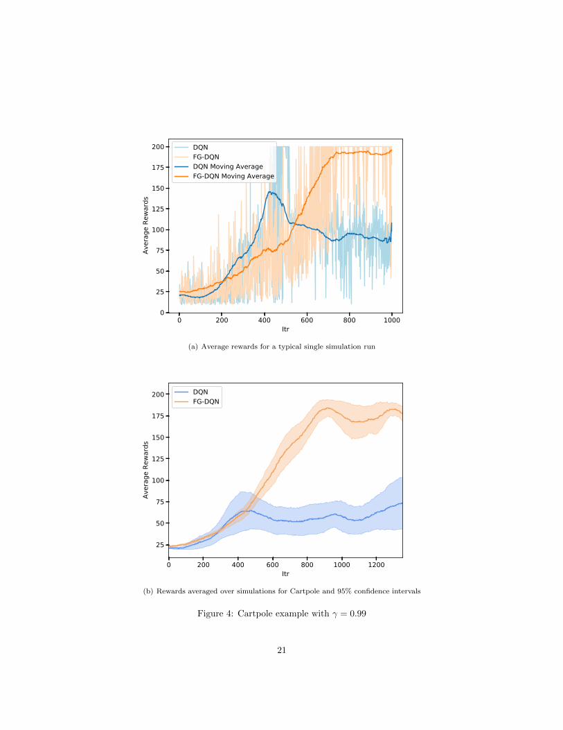
Fig.4(a) depicts the reward behaviour for a single typical run of DQN and FG-DQN. We seethat the fluctuations for reward per episode for both the algorithms are high, and thus, we alsoplot the moving average of rewards with a window of 100 episodes. It is clear from the figurethat FG-DQN starts achieving the maximum reward of 200 after 800 episodes regularly, how-ever, DQN hardly attains the maximum reward during 1000 episodes. To check the consistencyof the behaviour of our algorithm, we run the experiment 10 times and plot the average rewardand 95% confidence interval in Fig. 4(b). We see that FG-DQN performs much better thanDQN with an average reward after 1000 episodes lying around 175. In comparison, the averagereward for DQN is between 50 and 75.

20

0 200 400 600 800 1000Itr

0

25

50

75

100

125

150

175

200Av

erag

e Re

ward

sDQNFG-DQNDQN Moving AverageFG-DQN Moving Average

(a) Average rewards for a typical single simulation run

0 200 400 600 800 1000 1200Itr

25

50

75

100

125

150

175

200

Aver

age

Rewa

rds

DQNFG-DQN

(b) Rewards averaged over simulations for Cartpole and 95% confidence intervals

Figure 4: Cartpole example with γ = 0.99

21

6 Conclusions and future directions

We proposed and analyzed a variant of the popular DQN algorithm that we call Full GradientDQN or FG-DQN wherein we also include the parametric gradient (in a generalized sense) of thetarget. This leads to a provably convergent scheme with sound theoretical basis which also showsimproved performance over test cases. There is ample opportunity for further research in thisdirection, both theoretically and in terms of actual implementations. To highlight opportunities,we state here some additional remarks, which also contain a few pointers to future researchdirections.

1. Since the critical points are isolated, we get a.s. convergence to a single sample pathdependent critical point. This situation is generic in the sense that it holds true for theproblem parameters in an open dense set thereof, by a standard fact from Morse theoryin the smooth case. However, connected sets of non-isolated equilibria can occur due tooverparametrization and it will be interesting to develop sufficient conditions for pointconvergence.

2. Thanks to the addition of {ξn}, the noise in FG-DQN is ‘rich enough’ in all directionsin a certain sense. One then expects it to ensure that under reasonable assumptions, theunstable equilibria, here the critical points other than local minima of the Bellman error,will be avoided with probability one. That is, a.s. convergence to a local minimum can beclaimed. See section 4.3 of [9] for a result of this flavor under suitable technical conditions.We expect a similar result to hold here. In practice, the extraneous noise {ξn} is usuallyunnecessary and the inherent numerical errors and noise of the iterations suffice.

3. We can also use approximation of the ‘max’ operator by ‘softmax’, i.e., by picking thecontrol with a probability distribution that concentrates on argmax and depends smoothlyon the parameter θ. Then we can work with a legitimate gradient in place of a set-valuedmap in the o.d.e. limit, at the expense of picking up an additional bounded error term.Then the convergence to a small neighborhood of an equilibrium may be expected, thesize of which will be dictated in turn by the bound on this error, see, e.g., [34]. There is asimilar issue if we drop (C3) and let a persistent small error due to the use of approximateconditional expectation by experience replay remain.

4. Working with nondifferentiable nonlinearities such as ReLU raises further technical issuesin analysis that need to be explored. This will require further use of non-smooth analysis.

5. As we have pointed out while describing our numerical experiments on the cartpole exam-ple, FG-DQN gives a significantly better performance than DQN, in an ‘on-policy’ scenariofor which we do not have rigorous theory yet. This is another promising and importantresearch direction for the future.

7 Acknowledgement

The authors are greatly obliged to Prof. K. S. Mallikarjuna Rao for pointers to the relevantliterature on non-smooth analysis. The work of VSB was supported in part by an S. S. BhatnagarFellowship from the Council of Scientific and Industrial Research, Government of India. Thework of KP and KA is partly supported by ANSWER project PIA FSN2 (P15 9564-266178

22

/ DOS0060094) and the project of Inria - Nokia Bell Labs “Distributed Learning and Controlfor Network Analysis”. This work is also partly supported by the project IFC/DST-Inria-2016-01/448 “Machine Learning for Network Analytics”.

This is the author’s version of the work for the Springer book: A.B. Piunovskiy and Y. Zhang(eds.), Modern Trends in Controlled Stochastic Processes: Theory and Applications, Volume III,2021.

Appendix: Elements of non-smooth analysis

The (Frechet) sub/super-differentials of a map f : Rd 7→ R are defined by

∂−f(x) :=

{z ∈ Rd : lim inf

y→x

f(y)− f(x)− 〈z, y − x〉|x− y|

≥ 0

},

∂+f(x) :=

{z ∈ Rd : lim sup

y→x

f(y)− f(x)− 〈z, y − x〉|x− y|

≤ 0

},

respectively. Assume f, g is Lipschitz. Some of the properties of ∂±f are as follows.

• (P1) Both ∂−f(x), ∂+f(x) are closed convex and are nonempty on dense sets.

• (P2) If f is differentiable at x, both equal the singleton {∇f(x)}. Conversely, if both arenonempty at x, f is differentiable at x and they equal {∇f(x)}.

• (P3) ∂−f + ∂−g ⊂ ∂−(f + g), ∂+f + ∂+g ⊂ ∂+(f + g).

The first two are proved in [3], pp. 30-1. The third follows from the definition. Next considera continuous function f : Rd × B 7→ R where B is a compact metric space. Suppose f(·, y) iscontinuously differentiable uniformly w.r.t. y. Let ∇xf(x, y) denote the gradient of f(·, y) at x.Let g(x) := maxy f(x, y), h(x) := miny f(x, y) with

M(x) := {∇xf(x, y), y ∈ Argmaxf(x, ·)}

andN(x) := {∇xf(x, y), y ∈ Argminf(x, ·)}.

Then N(x),M(x) are compact nonempty subsets of B which are upper semicontinous in x asset-valued maps. We then have the following general version of Danskin’s theorem [15]:

• (P4) ∂−g(x) = co(M(x)), ∂+g(x) = y if M(x) = {y}, = φ otherwise, and g has a direc-tional derivative in any direction z given by maxy∈M(x)〈y, z〉.

• (P5) ∂+h(x) = co(N(x)), ∂−h(x) = y if N(x) = {y}, = φ otherwise, and h has a direc-tional derivative in any direction z given by miny∈N(x)〈y, z〉.

The latter is proved in [3], pp. 44-6, the former follows by a symmetric argument.

23

References

[1] Agarwal, A., Kakade, S.M., Jason D. L., Mahajan, G.: Optimality and approximation withpolicy gradient methods in Markov decision processes. In Conference on Learning Theory,PMLR, 64-66 (2020)

[2] Agazzi, A., Lu, J.: Global optimality of softmax policy gradient with single hidden layerneural networks in the mean-field regime. arXiv preprint arXiv:2010.11858, (2020)

[3] Bardi, M., Capuzzo-Dolcetta, I.: Optimal Control and Viscosity Solutions of Hamilton-Jacobi-Bellman Equations. Birkhauser, Boston (2018)

[4] Barto, A. G., Sutton, R. S., Anderson, C. W.: Neuronlike adaptive elements that can solvedifficult learning control problems. IEEE Trans. Syst. Man Cybern. Syst., 5, 834-846 (1983)

[5] Benveniste, A., Metivier, M., Priouret, P.: Adaptive Algorithms and Stochastic Approxi-mations. Springer Verlag, Berlin Heidelberg (1991)

[6] Bertsekas, D. P.: Reinforcement Learning and Optimal Control. Athena Scientific. (2019)

[7] Bhandari, J., Russo, D.: Global optimality guarantees for policy gradient methods. arXivpreprint arXiv:1906.01786. (2019)

[8] Borkar, V. S.: Probability Theory: An Advanced Course, Springer Verlag, New York.(1995)

[9] Borkar, V. S.: Stochastic Approximation: A Dynamical Systems Viewpoint. HindustanPublishing Agency, New Delhi, and Cambridge University Press, Cambridge, UK (2008)

[10] Brockman, G., Cheung, V., Pettersson, L., Schneider, J., Schulman, J., Tang, J., Zaremba,W.: OpenAI Gym. ArXiv preprint arXiv:1606.01540 (2016)

[11] Cai, Q., Yang, Z., Lee, J. D., Wang, Z.: Neural temporal-difference learning converges toglobal optima. Advances in Neural Information Processing Systems 32, (2019)

[12] Chades, I., Chapron, G., Cros, M. J., Garcia, F., Sabbadin, R.: MDPtoolbox: A multi-platform toolbox to solve stochastic dynamic programming problems. Ecography, 37, 916-920 (2014)

[13] Chizat, L., Bach, F.: On the global convergence of gradient descent for over-parameterizedmodels using optimal transport. In Proceedings of Neural Information Processing Systems,3040-3050 (2018)

[14] Couture, S., Cros, M. J., and Sabbadin R.: Risk aversion and optimal management of anuneven-aged forest under risk of windthrow: A Markov decision process approach. J. For.Econ. 25, 94-114 (2016)

[15] Danskin, J. M.: The theory of max-min, with applications. SIAM J. Appl. Math. 14,641-664 (1966)

[16] Delyon, B., Lavielle, M. and Moulines, E.: Convergence of a stochastic approximationversion of the EM algorithm. Ann. Stat. 27, pp. 94-128 (1999)

24

[17] Florian, R. V.: Correct equations for the dynamics of the cart-pole system. Center forCognitive and Neural Studies (Coneural), Romania (2007)

[18] Francois-Lavet, V., Henderson, P., Islam, R., Bellemare, M. G., Pineau, J.: An Introductionto Deep Reinforcement Learning. Found. Trends Mach. Learn. 11 3-4 pp. 219-354 (2018)

[19] Gordon, G. J.: Stable fitted reinforcement learning. Advances in Neural Information Pro-cessing Systems, pp.1052-1058 (1996)

[20] Gordon, G. J.: Approximate Solutions to Markov Decision Processes. PhD Thesis,Carnegie-Mellon University (1999)

[21] Gu, S., Holly, E., Lillicrap, T., Levine, S.: Deep reinforcement learning for robotic ma-nipulation with asynchronous off-policy updates. In Proceedings of IEEE InternationalConference on Robotics and Automation, 3389-3396 (2017)

[22] Haarnoja, T., Ha, S., Zhou, A., Tan, J., Tucker, G., Levine, S.: Learning to walk via deepreinforcement learning. ArXiv preprint arXiv:1812.11103 (2018)

[23] Jaakola, T., Jordan, M. I., Singh, S. P.: On the convergence of stochastic iterative dynamicprogramming algorithms. Neural Computation. 6, 1185–1201 (1994)

[24] Jonsson, A.: Deep reinforcement learning in medicine. Kidney Diseases 5, 18-22 (2019)

[25] Lin, L.J.: Self-improving reactive agents based on reinforcement learning, planning andteaching. Machine learning 8 3-4, 293-321 (1992)

[26] Lin, L.-J.: Reinforcement Learning for Robots Using Neural Networks., Ph.D. Thesis Schoolof Computer Science, Carnegie-Mellon University, Pittsburgh (1993)

[27] Luong, N. C., Hoang, D. T., Gong, S., Niyato, D., Wang, P., Liang, Y. C., Kim, D. I.:Applications of deep reinforcement learning in communications and networking: A survey.IEEE Commun. Surv. Tutor. 21, 3133-3174 (2019)

[28] Marbach, P., Tsitsiklis, J. N.: Simulation-based optimization of Markov reward processes.IEEE Trans. Automat. Contr. 46, 191-209 (2001)

[29] Mnih, V., Kavukcuoglu, K., Silver, D., Graves, A., Antonoglou, I., Wierstra, D., Riedmiller,M.: Playing Atari with deep reinforcement learning. arXiv preprint arXiv:1312.5602 (2013)

[30] Mnih, V., Kavukcuoglu, K., Silver, D., Rusu, A. A., Veness, J., Bellemare, M. G., Graves,A., Riedmiller, M., Fidjeland, A. K., Ostrovski, G., Petersen, S.: Human-level controlthrough deep reinforcement learning. Nature 518, 529-533 (2015)

[31] Peng, X. B., Berseth, G., Yin, K., van de Panne, M. Deeploco: Dynamic locomotion skillsusing hierarchical deep reinforcement learning. ACM Trans. Graph. 36, 1-13 (2017)

[32] Popova, M., Isayev, O., and Tropsha, A.: Deep reinforcement learning for de novo drugdesign. Sci. Adv. 4(7), eaap7885 (2018)

[33] Qian, Y., Wu, J., Wang, R., Zhu, F. and Zhang, W.: Survey on reinforcement learningapplications in communication networks. J. Commun. Netw. 4, 30-39 (2019)

25

[34] Ramaswamy, A., Bhatnagar, S.: Analysis of gradient descent methods with nondiminishingbounded errors. IEEE Trans. Automat. Contr. 63, 1465-1471 (2018)

[35] Riedmiller, M.: Neural fitted Q iteration–first experiences with a data efficient neuralreinforcement learning method. Machine Learning: ECML, pp. 317-328 (2005)

[36] Schaul, T., Quan, J., Antonoglou, I., Silver, D.: Prioritized experience replay. arXivpreprint arXiv:1511.05952 (2015)

[37] Silver, D., Huang, A., Maddison, C. J., Guez, A., Sifre, L., van den Driessche, G., Hassabis,D.: Mastering the game of Go with deep neural networks and tree search. Nature, 529,pp.484-489 (2016)

[38] Silver, D., Hubert, T., Schrittwieser, J., Antonoglou, I., Lai, M., Guez, A., Hassabis, D.:A general reinforcement learning algorithm that masters chess, shogi, and Go throughself-play. Science, 362, 1140-1144 (2018)

[39] Sutton, R. S. and Barto, A. G.: Reinforcement Learning: An Introduction. 2nd edition,MIT Press, (2018)

[40] Sutton, R. S., McAllester, D. A., Singh, S. P., Mansour, Y.: Policy gradient methodsfor reinforcement learning with function approximation. In Neural Information ProcessingSystems Proceedings, pp.1057-1063 (1999)

[41] Tsitsiklis, J. N.: Asynchronous stochastic approximation and Q-learning. Machine learning16, 185-202 (1994)

[42] Tsitsiklis, J. N., Van Roy, B.: An analysis of temporal-difference learning with functionapproximation. IEEE Trans. Automat. Contr. 42, 674-690 (1997)

[43] van Hasselt, H.: Double Q-learning. Advances in Neural Information Processing Systems23, 2613-2621 (2010)

[44] van Hasselt, H., Guez, A., Silver, D.: Deep reinforcement learning with double Q-learning.In Proceedings of the 30th AAAI Conference on Artificial Intelligence, 30, 2094-2100 (2016)

[45] Watkins, C. J. C. H.: Learning from Delayed Rewards. Ph.D. Thesis, King’s College,University of Cambridge, UK (1989)

[46] Watkins, C. J., Dayan, P.: Q-learning. Machine learning 8 3-4, 279-292 (1992)

[47] Xiong, Z., Zhang, Y., Niyato, D., Deng, R., Wang, P., Wang, L. C.: Deep reinforcementlearning for mobile 5G and beyond: Fundamentals, applications, and challenges. IEEE Veh.Technol. Mag. 14, 44-52 (2019)

[48] Yaji, V.G., Bhatnagar, S.: Stochastic recursive inclusions with non-additive iterate-dependent Markov noise. Stochastics, 90, 330-363 (2018)

26