HAL Id: hal-01091747https://hal.inria.fr/hal-01091747

Submitted on 6 Dec 2014

HAL is a multi-disciplinary open accessarchive for the deposit and dissemination of sci-entific research documents, whether they are pub-lished or not. The documents may come fromteaching and research institutions in France orabroad, or from public or private research centers.

L’archive ouverte pluridisciplinaire HAL, estdestinée au dépôt et à la diffusion de documentsscientifiques de niveau recherche, publiés ou non,émanant des établissements d’enseignement et derecherche français ou étrangers, des laboratoirespublics ou privés.

Deadlock Detection in Linear Recursive ProgramsElena Giachino, Cosimo Laneve

To cite this version:Elena Giachino, Cosimo Laneve. Deadlock Detection in Linear Recursive Programs. Formal Methodsfor Executable Software Models - 14th International School on Formal Methods for the Design ofComputer, Communication, and Software Systems, 2014, Jun 2014, Bertinoro, Italy. pp.26 - 64,�10.1007/978-3-319-07317-0_2�. �hal-01091747�

Deadlock detection in linear recursive programs‹

Elena Giachino and Cosimo Laneve

Dept. of Computer Science and Egineering, Universita di Bologna – INRIA FOCUStgiachino,laneveu@cs.unibo.it

Abstract. Deadlock detection in recursive programs that admit dy-namic resource creation is extremely complex and solutions either giveimprecise answers or do not scale.We define an algorithm for detecting deadlocks of linear recursive pro-

grams of a basic model. The theory that underpins the algorithm is ageneralization of the theory of permutations of names to so-called muta-

tions, which transform tuples by introducing duplicates and fresh names.Our algorithm realizes the back-end of deadlock analyzers for object-oriented programming languages, once the association programs/basic-model-programs has been defined as front-end.

1 Introduction

Modern systems are designed to support a high degree of parallelism by en-suring that as many system components as possible are operating concurrently.Deadlock represents an insidious and recurring threat when such systems alsoexhibit a high degree of resource and data sharing. In these systems, deadlocksarise as a consequence of exclusive resource access and circular wait for accessingresources. A standard example is when two processes are exclusively holding adifferent resource and are requesting access to the resource held by the other. Inother words, the correct termination of each of the two process activities dependson the termination of the other. Since there is a circular dependency, terminationis not possible.

The techniques for detecting deadlocks build graphs of dependencies px, yqbetween resources, meaning that the release of a resource referenced by x de-pends on the release of the resource referenced by y. The absence of cycles in thegraphs entails deadlock freedom. The difficulties arise in the presence of infinite(mutual) recursion: consider, for instance, systems that create an unboundednumber of processes such as server applications. In such systems, process inter-action becomes complex and either hard to predict or hard to be detected duringtesting and, even when possible, it can be difficult to reproduce deadlocks andfind their causes. In these cases, the existing deadlock detection tools, in orderto ensure termination, typically lean on finite models that are extracted fromthe dependency graphs.

‹ Partly funded by the EU project FP7-610582 ENVISAGE: Engineering VirtualizedServices.

The most powerful deadlock analyzer we are aware of is TyPiCal, a tooldeveloped for pi-calculus by Kobayashi [20, 18, 16, 19]. This tool uses a clevertechnique for deriving inter-channel dependency information and is able to dealwith several recursive behaviors and the creation of new channels without usingany pre-defined order of channel names. Nevertheless, sinceTyPiCal is based onan inference system, there are recursive behaviors that escape its accuracy. Forinstance, it returns false positives when recursion is mixed up with delegation. Toillustrate the issue we consider the following deadlock-free pi-calculus factorialprogram

*factorial ?(n,(r,s)).

if n=0 then r?m. s!m else new t in

(r?m. t!(m*n)) | factorial !(n-1,(t,s))

In this code, factorial returns the value (on the channel s) by delegating thistask to the recursive invocation, if any. In particular, the initial invocation offactorial, which is r!1 | factorial!(n,(r,s)), performs a synchronizationbetween r!1 and the input r?m in the continuation of factorial?(n,(r,s)).In turn, this may delegate the computation of the factorial to a subsequentsynchronization on a new channel t. TyPiCal signals a deadlock on the twoinputs r?m because it fails in connecting the output t!(m*n) with them.

The technique we develop in this paper allows us to demonstrate the deadlockfreedom of programs like the one above.

To ease program reasoning, our technique relies on an abstraction processthat extracts the dependency constraints in programs

– by dropping primitive data types and values;

– by highlighting dependencies between pi-calculus actions;

– by overapproximating statement behaviors, namely collecting the dependen-cies and the invocations in the two branches of the conditional (the set unionoperation is modeled by N).

This abstraction process is currently performed by a formal inference system thatdoes not target pi-calculus, but it is defined for a Java-like programming lan-guage, called ABS [17], see Section 6. Here, pi-calculus has been considered for ex-pository purposes. The ABS program corresponding to the pi-calculus factorialmay be downloaded from [15]; readers that are familiar with Java may find thecode in the Appendix A. As a consequence of the abstraction operation we getthe function

factorialpr, sq “ pr, sqNpr, tqNfactorialpt, sq

where pr, sq shows the dependency between the actions r?m and s!m and pr, tqthe one between r?m and t!(m*n). The semantics of the abstract factorial isdefined operationally by unfolding the recursive invocations. In particular, theunfolding of factorialpr, sq yields the sequence of abstract states (free namesin the definition of factorial are replaced by fresh names in the unfoldings)

2

factorialpr, sq ÝÑ pr, sqNpr, tqNfactorialpt, sqÝÑ pr, sqNpr, tqNpt, sqNpt, uqNfactorialpu, sqÝÑ pr, sqNpr, tqNpt, sqNpt, uqNpu, sqNpu, vq

Nfactorialpv, sqÝÑ ¨ ¨ ¨

We demonstrate that the abstract factorial (and, therefore, the foregoingpi-calculus code) never manifests a circularity by using a model checking tech-nique. This despite the fact that the model of factorial has infinite states.In particular, we are able to decide the deadlock freedom by analyzing finitelymany states – precisely three – of factorial.

Our solution. We introduce a basic recursive model, called lam programs – lamis an acronym for deadLock Analysis Model – that are collections of functiondefinitions and a main term to evaluate. For example,`

factorialpr, sq “ pr, sqNpr, tqNfactorialpt, sq , factorialpr, sq˘

defines factorial and the main term factorialpr, sq. Because lam programsfeature recursion and dynamic name creation – e.g. the free name t in the defi-nition of factorial – the model is not finite state (see Section 3).

In this work we address the

Question 1. Is it decidable whether the computations of a lam program will everproduce a circularity?

and the main contribution is the positive answer when programs are linear re-cursive.

To begin the description of our solution, we notice that, if lam programs arenon-recursive then detecting circularities is as simple as unfolding the invocationsin the main term. In general, as in case of factorial, the unfolding may notterminate. Nevertheless, the following two conditions may ease our answer:

(i) the functions in the program are linear recursive, that is (mutual) recursionshave at most one recursive invocation – such as factorial;

(ii) function invocations do not show duplicate arguments and function defini-tions do not have free names.

When (i) and (ii) hold, as in the program`fpx, y, zq “ px, yqNfpy, z, xq, fpu, v, wq

˘,

recursive functions may be considered as permutations of names – technicallywe define a notion of associated (per)mutation – and the corresponding the-ory [8] guarantees that, by repeatedly applying a same permutation to a tuple ofnames, at some point, one obtains the initial tuple. This point, which is knownas the order of the permutation, allows one to define the following algorithm forQuestion 1:

1. compute the order of the permutation associated to the function in the lamand

2. correspondingly unfold the term to evaluate.

3

For example, the permutation of f has order 3. Therefore, it is possible to stopthe evaluation of f after the third unfolding (at the state pu, vqNpv, wqNpw, uqN fpu, v, wq) because every dependency pair produced afterwards will belong tothe relation pu, vqNpv, wqNpw, uq.

When the constraint (ii) is dropped, as in factorial, the answer to Ques-tion 1 is not simple anymore. However, the above analogy with permutationshas been a source of inspiration for us.

order

(

g(x0, x1, x2, x3, x4, x5, x6) = (x3, x1)�(x0, x8)�(x8, x7)�g(x2, x0, x1, x5, x6, x7, x8), g(x0, x1, x2, x3, x�

g(x0, x1, x2, x3, x4, x5, x6)

(x3, x1)�(x0, x8)�(x8, x7) � g(x2, x0, x1, x5, x6, x7, x8)� � �

(x5, x0)�(x2, x10)�(x10, x9) � g(x1, x2, x0, x7, x8, x9, x10)� � �

(x7, x2)�(x1, x12)�(x12, x11) � g(x0, x1, x2, x9, x10, x11, x12)� � �

(x9, x1)�(x0, x14)�(x14, x13) � g(x2, x0, x1, x11, x12, x13, x14)� � �

(x11, x0)�(x2, x16)�(x16, x15) � g(x1, x2, x0, x13, x14, x15, x16)

, g(x0, x1, x2, x3, x4, x5, x6))

Fig. 1. A lam program and its unfolding

Consider the main term factorialpr, sq. Its evaluation will never displayfactorialpr, sq twice, as well as any other invocation in the states, becausethe first argument of the recursive invocation is free. Nevertheless, we noticethat, from the second state – namely pr, sqNpr, tqNfactorialpt, sq – onwards,the invocations of factorial are not identical, but may be identified by a mapthat

– associates names created in the last evaluation step to past names,– is the identity on other names.

The definition of this map, called flashback, requires that the transformation as-sociated to a lam function, called mutation, also records the name creation.In fact, the theory of mutations allows us to map factorialpt, sq back tofactorialpr, sq by recording that t has been created after r, e.g. răt.

We generalize the result about permutation orders (Section 2):

by repeatedly applying a same mutation to a tuple of names, at somepoint we obtain a tuple that is identical, up-to a flashback, to a tuple inthe past.

As for permutations, this point is the order of the mutation, which (we prove)it is possible to compute in similar ways.

4

However, unfolding a function as many times as the order of the associatedmutation may not be sufficient for displaying circularities. This is unsurprisingbecause the arguments about mutations and flashbacks focus on function invo-cations and do not account for dependencies. In the case of lams where (i) and(ii) hold, these arguments were sufficient because permutations reproduce thesame dependencies of past invocations. In the case of mutations, this is not trueanymore as displayed by the function g in Figure 1. This function has order 3and the first three unfoldings of gpx0, x1, x2, x3, x4, x5, x6q are those above thehorizontal line. While there is a flashback from gpx0, x1, x2, x9, x10, x11, x12q togpx0, x1, x2, x3, x4, x5, x6q, the pairs produced up-to the third unfolding

px3, x1qNpx0, x8qNpx8, x7qNpx5, x0qNpx2, x10qNpx10, x9qNpx7, x2qNpx1, x12qNpx12, x11q

do not manifest any circularity. Yet, two additional unfoldings (displayed belowthe horizontal line of Figure 1), show the circularity

px0, x8qNpx8, x7qNpx7, x2qNpx2, x10qNpx10, x9qNpx9, x1qNpx1, x12qNpx12, x11qNpx11, x0q .

flashback

L

(a)

L

flashback

L

(b)

L

saturated state= 2 order

circularity

order

saturated state= 2 order

circularity

order

Fig. 2. Flashbacks of circularities

In Section 4 we prove that a sufficient condition for deciding whether a lamprogram as in Figure 1 will ever produce a circularity is to unfold the function g

up-to two times the order of the associated mutation – this state will be calledsaturated. If no circularity is manifested in the saturated state then the lam is“circularity-free”. This supplement of evaluation is due to the existence of twoalternative ways for creating circularities. A first way is when the circularity isgiven by the dependencies produced by the unfoldings from the order to thesaturated state. Then, our theory guarantees that the circularity is also presentin the unfolding of g till the order – see Figure 2.a. A second way is when the

5

dependencies of the circularity are produced by (1) the unfolding till the orderand by (2) the unfolding from the order till the saturated state – these are theso-called crossover circularities – see Figure 2.b. Our theory allows us to mapdependencies of the evaluation (2) to those of the evaluation (1) and the flashbackmay break the circularity – in this case, the evaluation till the saturated stateis necessary to collect enough informations. Other ways for creating circularitiesare excluded. The intuition behind this fact is that the behavior of the function(the dependencies) repeats itself following the same pattern every order-wiseunfolding. Thus it is not possible to reproduce a circularity that crosses morethan one order without having already a shorter one. The algorithm for detectingcircularities in linear recursive lam programs is detailed in Section 5, togetherwith a discussion about its computational cost.

We have prototyped our algorithm [15]. In particular, the prototype (1) usesa (standard but not straightforward) inference system that we developed forderiving behavioral types with dependency informations out of ABS programs [13]and (2) has an add-on translationg these behavioral types into lams. We havebeen able to verify an industrial case study developed by SDL Fredhoppper –more than 2600 lines of code – in 31 seconds. Details about our prototype and acomparison with other deadlock analysis tools can be found in Section 6. Thereis no space in this contribution to discuss the inference system: the interestedreaders are referred to [13].

2 Generalizing permutations: mutations and flashbacks

Natural numbers are ranged over by a, b, i, j, m, n, . . . , possibly indexed. Let Vbe an infinite set of names, ranged over by x, y, z, ¨ ¨ ¨ . We will use partial orderrelations on names – relations that are reflexive, antisymmetric, and transitive –,ranged over by V,V1, I, ¨ ¨ ¨ . Let x P V if, for some y, either px, yq P V or py, xq P V.Let also varpVq “ tx | x P Vu. For notational convenience, we write rx when werefer to a list of names x1, . . . , xn.

Let V ‘ rxărz, with rx P V and rz R V, be the least partial order containing theset V Y tpy, zq | x P rx and px, yq P V and z P rzu. That is, rz become maximalnames in V ‘ rxărz. For example,

– tpx, xqu ‘ xăz “ tpx, xq, px, zq, pz, zqu;– if V “ tpx, yq, px1, y1qu (the reflexive pairs are omitted) then V ‘ yăz is thereflexive and transitive closure of tpx, yq, px1, y1q, py, zqu;

– if V “ tpx, yq, px, y1qu (the reflexive pairs are omitted) then V ‘ xăz is thereflexive and transitive closure of tpx, yq, px, y1q, py, zq, py1, zqu.

Let x ď y P V be px, yq P V.

Definition 1. A mutation of a tuple of names, denoted ( a1, ¨ ¨ ¨ , an ) where 1 ďa1, ¨ ¨ ¨ , an ď 2 ˆ n, transforms a pair

@V, px1, ¨ ¨ ¨ , xnq

Dinto

@V1, px1

1, ¨ ¨ ¨ , x1nq

D

as follows. Let tb1, ¨ ¨ ¨ , bku “ ta1, ¨ ¨ ¨ , anuzt1, 2, ¨ ¨ ¨ , nu and let zb1 , ¨ ¨ ¨ , zbk be k

pairwise different fresh names. [That is names not occurring either in x1, ¨ ¨ ¨ , xn

or in V.] Then

6

– if 1 ď ai ď n then x1i “ xai

;– if ai ą n then x1

i “ zai;

– V1 “ V ‘ x1, ¨ ¨ ¨ , xnăzi1 , ¨ ¨ ¨ , zik .

The mutation ( a1, ¨ ¨ ¨ , an ) of@V, px1, ¨ ¨ ¨ , xnq

Dis written

@V, px1, ¨ ¨ ¨ , xnq

D

( a1,¨¨¨ ,an )ÝÑ

@V1, px1

1, ¨ ¨ ¨ , x1nq

Dand the label ( a1, ¨ ¨ ¨ , an ) is omitted when the mu-

tation is clear from the context. Given a mutation µ “ ( a1, ¨ ¨ ¨ , an ), we definethe application of µ to an index i, 1 ď i ď n, as µpiq “ ai.

Permutations are mutations ( a1, ¨ ¨ ¨ , an ) where the elements are pairwise dif-ferent and belong to the set t1, 2, ¨ ¨ ¨ , nu (e.g. ( 2, 3, 5, 4, 1 )). In this case the par-tial order V never changes and therefore it is useless. Actually, our terminologyand statements below are inspired by the corresponding ones for permutations. Amutation differs from a permutation because it can exhibit repeated elements, oreven new elements (identified by n ` 1 ď ai ď 2 ˆ n, for some ai). For example,by successively applying the mutation ( 2, 3, 6, 1, 1 ) to

@V, px1, x2, x3, x4, x5q

D,

with V “ tpx1, x1q, ¨ ¨ ¨ , px5, x5qu and rx “ x1, x2, x3, x4, x5, we obtain@V, px1, x2, x3, x4, x5q

DÝÑ

@V1, px2, x3, y1, x1, x1q

D

ÝÑ@V2, px3, y1, y2, x2, x2q

D

ÝÑ@V3, py1, y2, y3, x3, x3q

D

ÝÑ@V4, py2, y3, y4, y1, y1q

D

ÝÑ ¨ ¨ ¨

where V1 “ V ‘ rxăy1 and, for i ě 1, Vi`1 “ Vi ‘ yiăyi`1. In this example, 6identifies a new name to be added at each application of the mutation. The newname created at each step is a maximal one for the partial order.

We observe that, by definition, ( 2, 3, 6, 1, 1 ) and ( 2, 3, 7, 1, 1 ) define a sametransformation of names. That is, the choice of the natural between 6 and10 is irrelevant in the definition of the mutation. Similarly for the mutations( 2, 3, 6, 1, 6 ) and ( 2, 3, 7, 1, 7 ).

Definition 2. Let ( a1, ¨ ¨ ¨ , an ) « ( a11, ¨ ¨ ¨ , a1

n ) if there exists a bijective func-tion f from rn ` 1..2 ˆ ns to rn ` 1..2 ˆ ns such that:

1. 1 ď ai ď n implies a1i “ ai;

2. n ` 1 ď ai ď 2 ˆ n implies a1i “ fpaiq.

We notice that ( 2, 3, 6, 1, 1 ) « ( 2, 3, 7, 1, 1 ) and ( 2, 3, 6, 1, 6 ) « ( 2, 3, 7, 1, 7 ).However ( 2, 3, 6, 1, 6 ) ff ( 2, 3, 6, 1, 7 ); in fact these two mutations define differenttransformations of names.

Definition 3. Given a partial order V, a V-flashback is an injective renamingρ on names such that ρpxq ď x P V.

In the above sequence of mutations of px1, x2, x3, x4, x5q there is a V4-flashbackfrom py2, y3, y4, y1, y1q to px2, x3, y1, x1, x1q. In the following, flashbacks will be

also applied to tuples: ρpx1, ¨ ¨ ¨ , xnqdef“ pρpx1q, ¨ ¨ ¨ , ρpxnqq.

7

In case of mutations that are permutations, a flashback is the identity renam-ing and the following statement is folklore. Let µ be a mutation. We write µm

for the application of µ m times, namely@V, px1, ¨ ¨ ¨ , xnq

D µm

ÝÑ@V1, py1, ¨ ¨ ¨ , ynq

D

abbreviates@V, px1, ¨ ¨ ¨ , xnq

D µÝÑ ¨ ¨ ¨

µÝÑ

@V1, py1, ¨ ¨ ¨ , ynq

Dlooooooooooooooooooooooooooooooomooooooooooooooooooooooooooooooon

m times

.

Proposition 1. Let µ “ ( a1, ¨ ¨ ¨ , an ) and@V, px1, ¨ ¨ ¨ , xnq

D µÝÑ

@V1, px1

1, ¨ ¨ ¨ , x1nq

Dµm

ÝÑ@V2, py1, ¨ ¨ ¨ , ynq

Dµ

ÝÑ@V3, py1

1, ¨ ¨ ¨ , y1nq

D

If there is a V2-flashback ρ such that ρpy1, ¨ ¨ ¨ , ynq “ px1, ¨ ¨ ¨ , xnq then thereis a V3-flashback from py1

1, ¨ ¨ ¨ , y1nq to px1

1, ¨ ¨ ¨ , x1nq.

Proof. Let ρ1 be the relation y1i ÞÑ x1

i, for every i. Then1) ρ1 is a mapping: y1

i “ y1j implies x1

i “ x1j . In fact, y1

i “ y1j means that either

(i) 1 ď ai, aj ď n or (ii) ai, aj ą n. In subcase (i) yai“ yaj

, by definition ofmutation. Therefore ρpyai

q “ ρpyajq that in turn implies xai

“ xaj. From this

last equality we obtain x1i “ x1

j . In subcase (ii), ai “ aj and the implicationfollows by the fact that ( a1, ¨ ¨ ¨ , an ) is a mutation.

2) ρ1 is injective: x1i “ x1

j implies y1i “ y1

j . If x1i P tx1, ¨ ¨ ¨ , xnu then 1 ď

ai, aj ď n. Therefore, by the definition of mutation, xai“ xaj

and, because ρ isa flashback, yai

“ yaj. By this last equation y1

i “ y1j . If x

1i R tx1, ¨ ¨ ¨ , xnu then

ai ą n and ai “ aj . Therefore y1i “ y1

j by definition of mutation.3) ρ1 is a flashback: x1

i ‰ y1i implies x1

i ď y1i P V3. If 1 ď ai ď n then y1

i “ yai

and x1i “ xai

. Therefore yai‰ xai

and we conclude by the hypothesis about ρ

that ρ1pyaiq satisfies the constraint in the definition of flashback. If ai ą n then

x1, ¨ ¨ ¨ , xn ď x1i P V1. Since ρpyiq “ xi, by the hypothesis about ρ, xi ď yi P V2.

Therefore, by definition of mutation, x1i ď yi P V2. We derive x1

i ď y1i P V3 by

transitivity because V2 Ď V3 and yi ď y1i P V3.

The following Theorem 1 generalizes the property that every permutationhas an order, which is the number of applications that return the initial tuple.In the theory of permutations, the order is the least common multiple, in shortlcm, of the lengths of the cycles of the permutation. This result is clearly falsefor mutations because of the presence of duplications and of fresh names. Thegeneralization that holds in our setting uses flashbacks instead of identities. Webegin by extending the notion of cycle.

Definition 4 (Cycles and sinks). Let µ “ ( a1, ¨ ¨ ¨ , an ) be a mutation andlet 1 ď ai1 , ¨ ¨ ¨ , aiℓ ď n be pairwise different naturals. Then:

i. the term pai1 ¨ ¨ ¨ aiℓq is a cycle of µ whenever µpaij q “ aij`1, with 1 ď j ď

ℓ´ 1, and µpaiℓq “ ai1 (i.e., pai1 ¨ ¨ ¨ aiℓq is the ordinary permutation cycle);ii. the term rai1 ¨ ¨ ¨ aiℓ´1

saiℓis a bound sink of µ whenever ai1 R ta1, ¨ ¨ ¨ , anu,

µpaij q “ aij`1, with 1 ď j ď ℓ ´ 1, and aiℓ belongs to a cycle;

8

iii. the term rai1 ¨ ¨ ¨ aiℓsa, with n ă a ď 2 ˆ n, is a free sink of µ wheneverai1 R ta1, ¨ ¨ ¨ , anu and µpaij q “ aij`1

, with 1 ď j ď ℓ ´ 1 and µpaiℓq “ a.

The length of a cycle is the number of elements in the cycle; the length of a sinkis the number of the elements in the square brackets.

For example the mutation ( 5, 4, 8, 8, 3, 5, 8, 3, 3 ) has cycle p3, 8q and has boundsinks r1, 5s3, r6, 5s3, r9s3, r2, 4s8, and r7s8. The mutation ( 6, 3, 1, 8, 7, 1, 8 ) hascycle p1, 6q, has bound sink r2, 3s1 and free sinks r4s8 and r5, 7s8.

Cycles and sinks are an alternative description of a mutation. For instancep3, 8q means that the mutation moves the element in position 8 to the element inposition 3 and the one in position 3 to the position 8; the free sink r5, 7s8 meansthat the element in position 7 goes to the position 5, whilst a fresh name goesin position 7.

Theorem 1. Let µ be a mutation, ℓ be the lcm of the length of its cycles, ℓ1 andℓ2 be the lengths of its longest bound sink and free sink, respectively. Let also

kdef“ maxtℓ`ℓ1, ℓ2u. Then there exists 0 ď h ă k such that

@V, px1, ¨ ¨ ¨ , xnq

D µh

ÝÑ@V1, py1, ¨ ¨ ¨ , ynq

D µk´h

ÝÑ@V2, pz1, ¨ ¨ ¨ , znq

Dand ρpz1, ¨ ¨ ¨ , znq “ py1, ¨ ¨ ¨ , ynq, for

some V2-flashback ρ. The value k is called order of µ and denoted by oµ.

Proof. Let µ “ ( a1, ¨ ¨ ¨ , an ) be a mutation, and letA “ t1, 2, . . . , nuzta1, ¨ ¨ ¨ , anu.If A “ ∅, then µ is a permutation; hence, by the theory of permutations, the

theorem is immediately proved taking ρ as the identity and h “ 0.If A ‰ ∅ then let a P A. By definition, a must be the first element of (i) a

bound sink or (ii) a free sink of µ. We write either a P Apiq or a P Apiiq if a isthe first element of a bound or free sink, respectively.

In subcase (i), let ℓ1a be the length of the bound sink with subscript a1 and

ℓa1 be the length of the cycle of a1. We observe that in@V, px1, ¨ ¨ ¨ , xnq

D µℓ1a

ÝÑ@U, px1

1, ¨ ¨ ¨ , x1nq

D µℓa1

ÝÑ@W, px2

1, ¨ ¨ ¨ , x2nq

Dwe have x1

a1 “ x2a1 .

In subcase (ii), let ℓ2a be the length of the free sink. We observe that in

@V, px1, ¨ ¨ ¨ , xnq

D µℓ2a

ÝÑ@U, px1

1, ¨ ¨ ¨ , x1nq

Dwe have xa ď x1

a P U, by definition ofmutation.

Let ℓ, ℓ1 and ℓ2 as defined in the theorem. Then, if ℓ ` ℓ1 ě ℓ2 we have that@V, px1, ¨ ¨ ¨ , xnq

D µℓ1

ÝÑ@V1, py1, ¨ ¨ ¨ , ynq

D µℓ

ÝÑ@V2, pz1, ¨ ¨ ¨ , znq

Dand ρpz1, ¨ ¨ ¨ , znq

“ py1, ¨ ¨ ¨ , ynq, where ρ “ rz1 ÞÑ y1, ¨ ¨ ¨ , zn ÞÑ yns is a V2-flashback. If ℓ `

ℓ1 ă ℓ2 then@V, px1, ¨ ¨ ¨ , xnq

D µℓ2´ℓ

ÝÑ@V1, py1, ¨ ¨ ¨ , ynq

D µℓ

ÝÑ@V2, pz1, ¨ ¨ ¨ , znq

D

and ρpz1, ¨ ¨ ¨ , znq “ py1, ¨ ¨ ¨ , ynq, where ρ “ rz1 ÞÑ y1, ¨ ¨ ¨ , zn ÞÑ yns is a V2-flashback.

For example, µ “ ( 6, 3, 1, 8, 7, 1, 8 ), has a cycle p1, 6q, bound sink r2, 3s1and free sinks r4s8 and r5, 7s8. Therefore ℓ “ 2, ℓ1 “ 2 and ℓ2 “ 2. In thiscase, the values k and h of Theorem 1 are 4 and 2, respectively. In fact, if we

9

apply the mutation µ four times to the pair@V, px1, x2, x3, x4, x5, x6, x7q

D, where

V “ tpxi, xiq | 1 ď i ď 7u we obtain@V, px1, x2, x3, x4, x5, x6, x7q

D µÝÑ

@V1, px6, x3, x1, y1, x7, x1, y1q

Dµ

ÝÑ@V2, px1, x1, x6, y2, y1, x6, y2q

Dµ

ÝÑ@V3, px6, x6, x1, y3, y2, x1, y3q

Dµ

ÝÑ@V4, px1, x1, x6, y4, y3, x6, y4q

D

where V1 “ V ‘ x1, x2, x3, x4, x5, x6, x7ăy1 and, for i ě 1, Vi`1 “ Vi ‘ yi´1ăyi.We notice that there is a V4-flashback ρ from px1, x1, x6, y4, y3, x6, y4q (producedby µ4) to px1, x1, x6, y2, y1, x6, y2q (produced by µ2).

3 The language of lams

We use an infinite set of function names, ranged over f, f1, g, g1,. . ., whichis disjoint from the set V of Section 2. A lam program is a tuple

`f1pĂx1q “

L1, ¨ ¨ ¨ , fℓp rxℓq “ Lℓ, L˘where fip rxiq “ Li are function definitions and L is the

main lam. The syntax of Li and L is

L ::“ 0 | px, yq | fprxq | LNL | L + L

Whenever parentheses are omitted, the operation “N” has precedence over“ + ”. We will shorten L1N¨ ¨ ¨ NLn into NiP1..nLi. Moreover, we use T to rangeover lams that do not contain function invocations.

Let varpLq be the set of names in L. In a function definition fprxq “ L, rx arethe formal parameters and the occurrences of names x P rx in L are bound ; thenames varpLqzrx are free.

In the syntax of L, the operations “N” and “ + ” are associative, commutativewith 0 being the identity. Additionally the following axioms hold (T does notcontain function invocations)

TNT “ T T + T “ T TNpL1 + L2q “ TNL1 + TNL2

and, in the rest of the paper, we will never distinguish equal lams. For instance,fpruq + px, yq and px, yq + fpruq will be always identified. These axioms permitto rewrite a lam without function invocations as a collection (operation + ) ofrelations (elements of a relation are gathered by the operation N).

Proposition 2. For every T, there exist T1, ¨ ¨ ¨ , Tn that are dependencies com-posed with N, such that T “ T1 + ¨ ¨ ¨ + Tn.

Remark 1. Lams are intended to be abstract models of programs that highlightthe resource dependencies in the reachable states. The lam T1 + ¨ ¨ ¨ + Tn ofProposition 2 models a program whose possibly infinite set of states tS1, S2, ¨ ¨ ¨ uis such that the resource dependencies in Si are a subset of those in some Tji , with1 ď ji ď n. With this meaning, generic lams L1 + ¨ ¨ ¨ + Lm are abstractions oftransition systems (a standard model of programming languages), where transi-tions are ignored and states record the resource dependencies and the functioninvocations.

10

Remark 2. The above axioms, such as TNpL1 + L2q “ TNL1 + TNL2 are re-stricted to terms T that do not contain function invocations. In fact, fpruqNppx, yq+ py, zqq ‰ pfpruqNpx, yqq + pfpruqNpy, zqq because the two terms have a differ-ent number of occurrences of invocations of f, and this is crucial for linearrecursion – see Definition 6.

In the paper, we always assume lam programs`f1pĂx1q “ L1, ¨ ¨ ¨ , fℓp rxℓq “

Lℓ, L˘to be well-defined, namely (1) all function names occurring in Li and L are

defined; (2) the arity of function invocations matches that of the correspondingfunction definition.

Operational semantics. Let a lam context, noted Lr s, be a term derived by thefollowing syntax:

Lr s ::“ r s | LNLr s | L + Lr s

As usual LrLs is the lam where the hole of Lr s is replaced by L. The opera-tional semantics of a program

`f1pĂx1q “ L1, ¨ ¨ ¨ , fℓp rxℓq “ Lℓ, Lℓ`1

˘is a transition

system whose states are pairs@V, L

Dand the transition relation is the least one

satisfying the rule:

(Red)

fprxq “ L varpLqzrx “ rz rw are freshLr rw{rzsrru{rxs “ L1

@V, Lrfpruqs

DÝÑ

@V ‘ ruă rw, LrL1s

D

By (red), a lam L is evaluated by successively replacing function invocationswith the corresponding lam instances. Name creation is handled with a mecha-nism similar to that of mutations. For example, if fpxq “ px, yqNfpyq and fpuqoccurs in the main lam, then fpuq is replaced by pu, vqNfpvq, where v is a freshmaximal name in some partial order. The initial state of a program with main

lam L is@IL, L

D, where IL

def“ tpx, xq | x P varpLqu.

To illustrate the semantics of the language of lams we discuss three examples:

1.`fpx, y, zq “ px, yqNgpy, zq + py, zq, gpu, vq “ pu, vq + pv, uq, fpx, y, zq

˘

and I “ tpx, xq, py, yq, pz, zqu. Then@I, fpx, y, zq

DÝÑ

@I, px, yqNgpy, zq + py, zq

D

ÝÑ@I, px, yqNpy, zq + px, yqNpz, yq + py, zq

D

The lam in the final state does not contain function invocations. This isbecause the above program is not recursive. Additionally, the evaluation offpx, y, zq has not created names. This is because names in the bodies offpx, y, zq and gpu, vq are bound.

2.`f1pxq “ px, yqNf1pyq , f1pxq

˘and V0 “ tpx0, x0qu. Then

@V0, f

1px0qD

ÝÑ@V1, px0, x1qNf1px1q

D

ÝÑ@V2, px0, x1qNpx1, x2qNf1px2q

D

ÝÑn@Vn`2, px0, x1qN¨ ¨ ¨ Npxn`1, xn`2qNf1pxn`2q

D

11

where Vi`1 “ Vi ‘ xiăxi`1. In this case, the states grow in the number ofdependencies as the evaluation progresses. This growth is due to the presenceof a free name in the definition of f1 that, as said, corresponds to generatinga fresh name at every recursive invocation.

3.`f2pxq “ px, x1q + px, x1qNf2px1q, f2px0q

˘and V0 “ tpx0, x0qu. Then@

V0, f2px0q

D

ÝÑ@V1, px0, x1q + px0, x1qNf2px1q

D

ÝÑ@V2, px0, x1q + px0, x1qNpx1, x2q + px0, x1qNpx1, x2qNf2px2q

D

ÝÑn@Vn`2, px0, x1q + ¨ ¨ ¨ + px0, x1qN¨ ¨ ¨ Npxn`1, xn`2qNf2pxn`2q

D

where Vi`1 are as before. In this case, the states grow in the number of“ + ”-terms, which become larger and larger as the evaluation progresses.

The semantics of the language of lams is nondeterministic because of thechoice of the invocation to evaluate. However, lams enjoy a diamond propertyup-to bijective renaming of (fresh) names.

Proposition 3. Let ı be a bijective renaming and ıpVq “ tpıpxq, ıpyqq | px, yq PVu. Let also

@V, L

DÝÑ

@V1, L1

Dand

@ıpVq, Lrıprxq{rxs

DÝÑ

@V2, L2

D, where

rx “ varpVq. Then

piq either there exists a bijective renaming ı1 such that

@V2, L2

D“

@ıpV1q, L1rıp rx1q{ rx1s

D,

where rx1 “ varpV1q,piiq or there exist L3 and a bijective renaming ı1 such that

@V1, L1

DÝÑ

@V3, L3

D

and@V2, L2

DÝÑ

@ı1pV3q, L3rı

1przq{rzsD, where rz “ varpV3q.

The informative operational semantics. In order to detect the circularity-freedom,our technique computes a lam till every function therein has been adequatelyunfolded (up-to twice the order of the associated mutation). This is formalizedby switching to an “informative” operational semantics where basic terms (de-pendencies and function invocations) are labelled by so-called histories.

Let a history, ranged over by α, β, ¨ ¨ ¨ , be a sequence of function namesfi1fi2 ¨ ¨ ¨ fin . We write f P α if f occurs in α. We also write αn for α ¨ ¨ ¨αloomoon

n times

. Let

α ĺ β if there is α1 such that αα1 “ β. The symbol ε denotes the empty history.The informative operational semantics is a transition system whose states

are tuples@V, hF, L

Dwhere hF is a set of function invocations with histories

and L, called informative lam, is a term as L, except that pairs and functioninvocations are indexed by histories, i.e. αpx, yq and αfpruq, respectively.

Let

addhpα, Lqdef“

$’’’’’’&’’’’’’%

αpx, yq if L “ px, yq

αfprxq if L “ fprxq

addhpα, L1qNaddhpα, L2q if L “ L1NL2

addhpα, L1q + addhpα, L2q if L “ L1 + L2

12

For example addhpfl, px4, x2qNfpx2, x3, x4, x5qq “ flpx4, x2qN flfpx2, x3, x4, x5q.Let also h

Lr s be a lam context with histories (dependency pairs and functioninvocations are labelled by histories, the definition is similar to Lr s).

The informative transition relation is the least one such that(Red+)

fprxq “ L varpLqzrx “ rz rw are freshLr rw{rzsrru{rxs “ L1

@V, hF, h

LrαfpruqsD

ÝÑ@V ‘ ruă rw, hF Y tαfpruqu, h

Lraddhpαf, L1qsD

When@V, hF, L

DÝÑ

@V1, hF1, L1

Dby applying (Red+) to αfpruq, we say

that the term αfpruq is evaluated in the reduction. The initial informative stateof a program with main lam L is

@IL, ∅, addhpε, Lq

D.

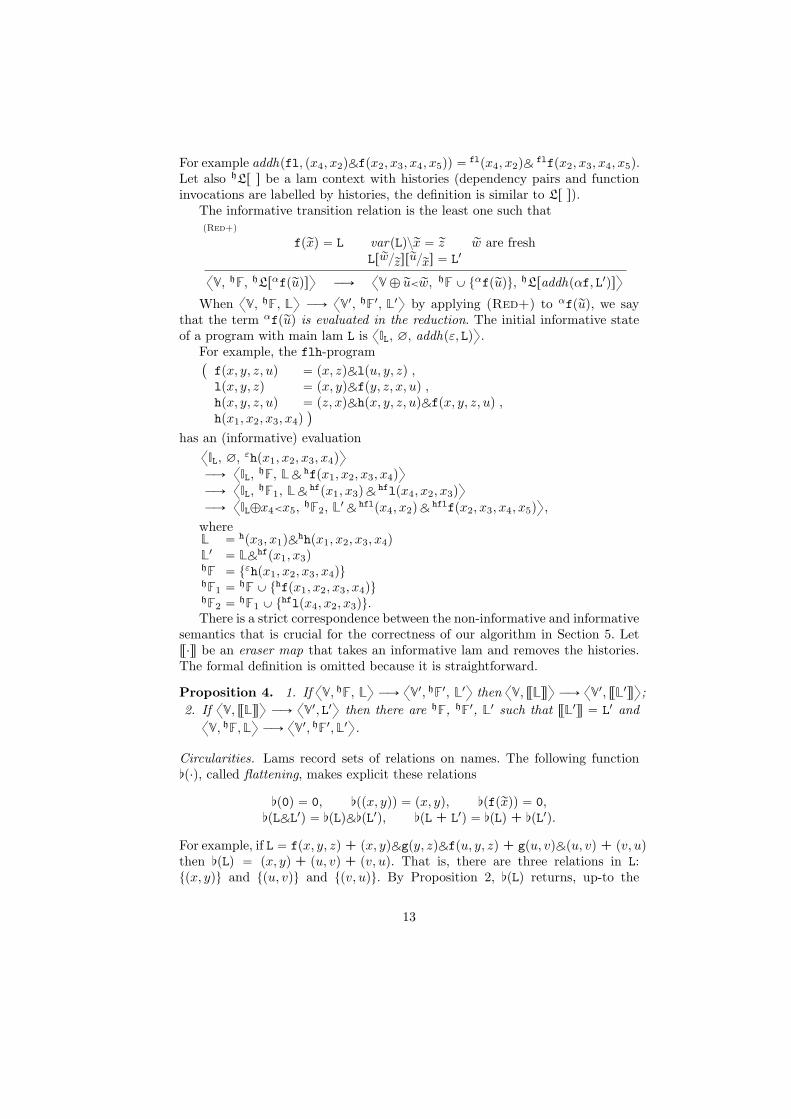
For example, the flh-program`fpx, y, z, uq “ px, zqNlpu, y, zq ,lpx, y, zq “ px, yqNfpy, z, x, uq ,hpx, y, z, uq “ pz, xqNhpx, y, z, uqNfpx, y, z, uq ,hpx1, x2, x3, x4q

˘

has an (informative) evaluation@IL, ∅, εhpx1, x2, x3, x4q

D

ÝÑ@IL,

hF, L Nhfpx1, x2, x3, x4q

D

ÝÑ@IL,

hF1, L Nhfpx1, x3q N

hflpx4, x2, x3qD

ÝÑ@IL‘x4ăx5,

hF2, L1N

hflpx4, x2q Nhflfpx2, x3, x4, x5q

D,

whereL “ hpx3, x1qNhhpx1, x2, x3, x4qL1 “ LN

hfpx1, x3qhF “ tεhpx1, x2, x3, x4quhF1 “ hF Y thfpx1, x2, x3, x4quhF2 “ hF1 Y thflpx4, x2, x3qu.There is a strict correspondence between the non-informative and informative

semantics that is crucial for the correctness of our algorithm in Section 5. Letrr¨ss be an eraser map that takes an informative lam and removes the histories.The formal definition is omitted because it is straightforward.

Proposition 4. 1. If@V, hF, L

DÝÑ

@V1, hF1, L1

Dthen

@V, rrLss

DÝÑ

@V1, rrL1ss

D;

2. If@V, rrLss

DÝÑ

@V1, L1

Dthen there are hF, hF1, L1 such that rrL1ss “ L1 and@

V, hF,LD

ÝÑ@V1, hF1,L1

D.

Circularities. Lams record sets of relations on names. The following function5p¨q, called flattening, makes explicit these relations

5p0q “ 0, 5ppx, yqq “ px, yq, 5pfprxqq “ 0,

5pLNL1q “ 5pLqN5pL1q, 5pL + L1q “ 5pLq + 5pL1q.

For example, if L “ fpx, y, zq + px, yqNgpy, zqNfpu, y, zq + gpu, vqNpu, vq + pv, uqthen 5pLq “ px, yq + pu, vq + pv, uq. That is, there are three relations in L:tpx, yqu and tpu, vqu and tpv, uqu. By Proposition 2, 5pLq returns, up-to the

13

lam axioms, sequences of (pairwise different) N-compositions of dependencies.The operation 5p¨q may be extended to informative lams L in the obvious way:5pαpx, yqq “ αpx, yq and 5pαfprxqq “ 0.

Definition 5. A lam L has a circularity if

5pLq “ px1, x2qNpx2, x3qN¨ ¨ ¨ Npxm, x1qNT1 + T2

for some x1, ¨ ¨ ¨ , xm. A state@V, L

Dhas a circularity if L has a circularity.

Similarly for an informative lam L.

The final state of the fgh-program computation has a circularity; another func-tion displaying a circularity is g in Section 1. None of the states in the examples1, 2, 3 at the beginning of this section has a circularity.

4 Linear recursive lams and saturated states

This section develops the theory that underpins the algorithm of Section 5.In order to lightening the section, the technical details have been moved inAppendix B.

We restrict our arguments to (mutually) recursive lam programs. In fact,circularity analysis in non-recursive programs is trivial: it is sufficient to evalu-ate all the invocations till the final state and verify the presence of circularitiestherein. A further restriction allows us to simplify the arguments without loosingin generality (cf. the definition of saturation): we assume that every function is(mutually) recursive. We may reduce to this case by expanding function invoca-tion of non-(mutually) recursive functions (and removing their definitions).

Linear recursive functions and mutations. Our decision algorithm relies on in-terpreting recursive functions as mutations. This interpretation is not alwayspossible: the recursive functions that have an associated mutation are the linearrecursive ones, as defined below.

The technique for dealing with the general case is briefly discussed in Sec-tion 8 and is detailed in Appendix C.

Definition 6. Let`f1pĂx1q “ L1, ¨ ¨ ¨ , fℓp rxℓq “ Lℓ, L

˘be a lam program. A se-

quence fi0fi1 ¨ ¨ ¨ fik is called a recursive history of fi0 if (a) the function namesare pairwise different and (b) for every 0 ď j ď k, Lij contains one invocationof fij`1%k

(the operation % is the remainder of the division).The lam program is linear recursive if (a) every function name has a unique

recursive history and (b) if fi0fi1 ¨ ¨ ¨ fik is a recursive history then, for every0 ď j ď k, Lij contains exactly one invocation of fij`1%k

.

For example, the program`f1px, yq “ px, yqNf1py, zqNf2pyq + f2pzq , f2pyq “ py, zqNf2pzq , L

˘

is linear recursive. On the contrary`fpxq “ px, yqNgpxq , gpxq “ px, yqNfpxq + gpyq , L

˘

14

is not linear recursive because g has two recursive histories, namely g and gf.Linearity allows us to associate a unique mutation to every function name.

To compute this mutation, let H range over sequences of function invocations.We use the following two rules:

fiα |ù ε fiprxiq “ Li

α |ù fiprxiq

fjα |ù Hfiprxq fiprxiq “ LivarpLiqzrxi “ rz rw are fresh

Lrfjpryqs “ Lir rw{rzsrrx{rxis

α |ù Hfiprxqfjpryq

Let ε |ù fpx1, ¨ ¨ ¨ , xnq ¨ ¨ ¨ fpx11, ¨ ¨ ¨ , x1

nq be the final judgment of the proof treewith leaf fαf |ù ε, where fα is the recursive history of f. Let also x1

1, ¨ ¨ ¨ , x1nzx1,

¨ ¨ ¨ , xn “ z1, ¨ ¨ ¨ , zk. Then the mutation of f, written µf “ ( a1, ¨ ¨ ¨ , an ) isdefined by

ai “

$&%

j if x1i “ xj

n ` j if x1i “ zj

Let of, called order of the function f, be the order of µf. For example, in theflh-program, the recursive history of f is fl and, applying the algorithm aboveto flf |ù ε, we get ε |ù fpx, y, z, uqlpu, y, zqfpy, z, u, vq. The mutation of f is( 2, 3, 4, 5 ) and of “ 4. Analogously we can compute ol “ 3 and oh “ 1.

Saturation. In the remaining part of the section we assume a fixed linearrecursive program

`f1pĂx1q “ L1, ¨ ¨ ¨ , fℓp rxℓq “ Lℓ, L

˘and let of1 , ¨ ¨ ¨ , ofℓ be the

orders of the corresponding functions.

Definition 7. A history α is

f-complete

if α “ βof , where β is the recursive history of f. We say that α is completewhen it is f-complete, for some f.

f-saturatingif α “ β1 ¨ ¨ ¨βn´1α

2n, where βi ĺ pαiq

2, with αi complete, and αn f-complete.We say that α is saturating when it is f-saturating, for some f.

In the flh-program, of “ 4, ol “ 3, and oh “ 1, and the recursive histories off, l and h are equal to fl, to lf and to h, respectively. Then α “ pflq4 is thef-complete history and h2pflq8 and hpflq8 are f-saturating.

The following proposition is an important consequence of the theory of mu-tations (Theorem 1) and the semantics of lams (and their axioms). In particular,it states that, if a function invocation f0pĂu0q is unfolded up to the order of f0then (i) the last invocation f0prvq may be mapped back to a previous invocationby a flashback and (ii) the same flashback also maps back dependencies createdby the unfolding of f0prvq.

Proposition 5. Let β “ f0f1 ¨ ¨ ¨ fn be f0-complete and let@V, hF, h

L0rαf0pĂu0qsD

ÝÑn`1@V1, hF1, h

L0rhL1r¨ ¨ ¨ hLnrαf0¨¨¨fnf0pĆun`1qs ¨ ¨ ¨ ssD

15

where hF1 “ hF Y tαf0pĂu0q, αf0f1pĂu1q, ¨ ¨ ¨ , αf0¨¨¨fn´1fnpĂunqu and fip ruiq “ L1i and

addhpαf0 ¨ ¨ ¨ fi, L1iq “ h

Lirαf0¨¨¨fifi`1pĆui`1qs (unfolding of the functions in the

complete history of f0). Then there is a αf0¨¨¨fh´1fhpĂuhq P hF1 and a V1-flashbackρ such that

1. f0pρpĆun`1qq “ fhpĂuhq (hence f0 “ fh);2. let f0pĆun`1q “ L and 5pLq “ T1 + ¨ ¨ ¨ + Tk and

5phL0rhL1r¨ ¨ ¨ hLnrαβf0pĆun`1qs ¨ ¨ ¨ ssq “ hT11+ ¨ ¨ ¨ + hT1

k1 . Then, for every1 ď i ď k, there exists 1 ď j ď k1 such that hT1

j “ addhpαf0 ¨ ¨ ¨ fh´1, TiqNhT2

j ,

for some hT2j .

The notion of f-saturating will be used to define a “saturated” state, i.e., astate where the evaluation of programs may safely (as regards circularities) stop.

Definition 8. An informative lam@V, hF, L

Dis saturated when, for every h

Lr s

and fpruq such that L “ hLrαfpruqs, α has a saturating prefix.

It is easy to check that the following informative lam generated by the com-putation of the flh-program is saturated:

@V7,

hF, h2

hpx1, x2, x3, x4q N N0ďiď8hfplfqipxi`1, xi`3q

N N0ďiď8hpflqipxi`3, xi`1q

Nhpflq8fpx9, x10, x11, x12q

D,

where Vi`1 “ Vi ‘ xi`4ăxi`5, andhF “ tεhpx1, x2, x3, x4q, hhpx1, x2, x3, x4qu

Ythpflqifpxi`1, xi`2, xi`3, xi`4q | 0 ď i ď 7u

Y thfplfqilpxi`4, xi`2, xi`3q | 0 ď i ď 7u.

Every preliminary statement is in place for our key theorem that detailsthe mapping of circularities created by transitions of saturated states to pastcircularities.

Theorem 2. Let@IL, ∅, addhpε, Lq

DÝÑ˚

@V, hF, L

Dand

@V, hF, L

Dbe a sat-

urated state. If@V, hF, L

DÝÑ

@V1, hF1, L1

Dthen

1.@V1, hF1, L1

Dis saturated;

2. if L1 has a circularity then L has already a circularity.

Proof. (Sketch) Item 1. directly follows from Proposition 5. However, this propo-sition is not sufficient to guarantee that circularities created in saturated statesare mapped back to past ones. In particular, the interesting case is the one ofcrossover circularities, as discussed in Section 1. Therefore, let

α1px1, x2q, ¨ ¨ ¨ , αh´1pxh´1, xhq, αhpxh, xh`1q, ¨ ¨ ¨ , αnpxn, x1q

be a circularity in L1 such that αhpxh, xh`1q, ¨ ¨ ¨ , αnpxn, x1q were already presentin L. Proposition 5 guarantees the existence of a flashback ρ that maps α1px1, x2qN¨ ¨ ¨ Nαh´1pxh´1, xhq to α1pρpx1q, ρpx2qqN¨ ¨ ¨ Nαh´1pρpxh´1q, ρpxhqq. However, itis possible that

16

α1pρpx1q, ρpx2qqN¨ ¨ ¨ Nαh´1pρpxh´1q, ρpxhqqNαhpxh, xh`1qN¨ ¨ ¨ Nαnpxn, x1q

is no more a circularity because, for example, ρpxhq ‰ xh (assume that ρpx1q “x1). Let us discuss this issue. The hypothesis of saturation guarantees that tran-sitions produce histories α2β, where α is complete. Additionally, α1, ¨ ¨ ¨ , αh´1

must be equal because they have been created by@V, hF, L

DÝÑ

@V1, hF1, L1

D.

For simplicity, let β “ f and α “ fα1. Therefore, by Proposition 5, ρ mapsα2

fpx1, x2qN¨ ¨ ¨ N α2fpxh´1, xhq to αfpρpx1q, ρpx2qqN¨ ¨ ¨ Nαfpρppxh´1q, ρpxhqq and,

ρpxhq ‰ xh when xh is created by the computation evaluating functions in α1.To overcome this problem, it is possible to demonstrate using a statement

similar to (but stronger than) Proposition 5 that ρ maps αhpxh, xh`1q N ¨ ¨ ¨N

αnpxn, x1q to rαhspρpxhq, ρpxh`1qqN¨ ¨ ¨ Nrαnspρpxnq, ρpx1qq where rαis are “ker-nels” of αi where every γk in αi, with γ a complete history and k ě 2, is replacedby γ. The proof terminates by demonstrating that the term

αfpρpx1q, ρpx2qqN¨ ¨ ¨ Nαfpρppxh´1q, ρpxhqqN

rαhspρpxhq, ρpxh`1qqN¨ ¨ ¨ Nrαnspρpxnq, ρpx1qq

is in L (and it is a circularity).

5 The decision algorithm for detecting circularities in

linear recursive lams

The algorithm for deciding the circularity-freedom problem in linear recursivelam programs takes as input a lam program

`f1pĂx1q “ L1, ¨ ¨ ¨ , fℓp rxℓq “ Lℓ, L

˘

and performs the following steps:

Step 1: find recursive histories. By parsing the lam program we create a graphwhere nodes are function names and, for every invocation of g in the body of f,there is an edge from f to g. Then a standard depth first search associates toevery node its recursive histories (the paths starting and ending at that node, ifany). The lam program is linear recursive if every node has at most one associatedrecursive history.

Step 2: computation of the orders. Given the recursive history α associated toa function f, we compute the corresponding mutation by running α |ù ε (seeSection 4). A straightforward parse of the mutation returns the set of cycles andsinks and, therefore, gives the order of.

Step 3: evaluation process. The main lam is unfolded till the the saturated state.That is, every function invocation fprxq in the main lam is evaluated up-to twicethe order of the corresponding mutation. The function invocation of f in thesaturated state is erased and the process is repeated on every other functioninvocation (which, therefore, does not belong to the recursive history of f), tillno function invocation is present in the state. At this stage we use the lam axiomsthat yield a term T1 + ¨ ¨ ¨ + Tn.

Step 4: detection of circularities. Every Ti in T1 + ¨ ¨ ¨ + Tn may be representedas a graph where nodes are names and edges correspond to dependency pairs. To

17

detect whether Ti contains a circular dependency, we run Tarjan algorithm [31]for connected components of graphs and we stop the algorithm when a circularityis found.

Every preliminary notion is in place for stating our main result; we also makefew remarks about the correctness of the algorithm and its computational cost.

Theorem 3. The problem of the circularity-freedom of a lam program is decid-able when the program is linear recursive.

The algorithm consists of the four steps described above. The critical step, asfar as correctness is concerned, is the third one, which follows by Theorem 2 andby the diamond property in Proposition 3 (whatever other computation may becompleted in such a way the final state is equal up-to a bijection to a saturatedstate).

As regards the computational complexity Steps 1 and 2 are linear withrespect to the size of the lam program and Step 4 is linear with respect to thesize of the term T1 + ¨ ¨ ¨ + Tn. Step 3 evaluates the program till the saturatedstate. Let

omax be the largest order of a function;mmax be the maximal number of function invocations in a body, apart the one

in the recursive history.

Without loss of generality, we assume that recursive histories have length 1 andthat the main lam consists of mmax invocations of the same function. Then anupper bound to the length of the evaluation till the saturated state is

p2 ˆ omax ˆ mmax q ` p2 ˆ omax ˆ mmax q2 ` ¨ ¨ ¨ ` p2 ˆ omax ˆ mmax qℓ

Let kmax be the maximal number of dependency pairs in a body. Then the size ofthe saturated state is Opkmax ˆpomax ˆ mmax qℓq, which is also the computationalcomplexity of our algorithm.

6 Assessments

The algorithm defined in Section 5 has been prototyped [15]. As anticipated inSection 1, our analysis has been applied to a concurrent object-oriented languagecalled ABS [17], which is a Java-like language with futures and an asynchronousconcurrency model (ASP [6] is another language in the same family).

The prototype is part of a bigger framework for the deadlock analysis of ABSprograms called DF4ABS (Deadlock Framework for ABS). It is a modular frame-work which includes two different approaches for analysing lams: DF4ABS/model-check (which is the one described in the current paper) and DF4ABS/fixpoint

(which is the one described in [13, 14]).The technique underpinning the DF4ABS/fixpoint tool derives the depen-

dency graph(s) of lam programs by means of a standard fixpoint analysis. To

18

circumvent the issue of the infinite generation of new names, the fixpoint is com-puted on models with a limited capacity of name creation. This introduces over-approximations that in turn display false positives (for example, DF4ABS/fix-point returns a false positive for the lam of factorial). In the present work,this limitation of finite models is overcome (for linear recursive programs) byrecognizing patterns of recursive behaviors, so that it is possible to reduce theanalysis to a finite portion of computation without losing precision in the detec-tion of deadlocks.

The derivation of lams from ABS programs is defined by an inference sys-tem [13, 14]. The inference system extracts behavioral types from ABS programsand feeds them to the analyzer. These types display the resource dependenciesand the method invocations while discarding irrelevant (for the deadlock analy-sis) details. There are two relevant differences between inferred types and lams:(i) methods’ arguments have a record structure and (ii) behavioral types havethe union operator (for modeling the if-then-else statement). To bridge this gapand have some initial assessments, we perform a basic automatic transformationof types into lams.

We tested our prototype on a number of medium-size programs written forbenchmarking purposes by ABS programmers and on an industrial case studybased on the Fredhopper Access Server (FAS) developed by SDL Fredhopp-per [9]. This Access Server provides search and merchandising IT services toe-Commerce companies. The (leftmost three columns of the) following table re-ports the experiments: for every program we display the number of lines, whetherthe analysis has reported a deadlock (D) or not (X), the time in seconds requiredfor the analysis. Concerning time, we only report the time of the analysis (andnot the one taken by the inference) when they run on a QuadCore 2.4GHz andGentoo (Kernel 3.4.9):

program linesDF4ABS/model-check

result timeDF4ABS/fixpoint

result timeDECO

result timePingPong 61 X 0.311 X 0.046 X 1.30MultiPingPong 88 D 0.209 D 0.109 D 1.43BoundedBuffer 103 X 0.126 X 0.353 X 1.26PeerToPeer 185 X 0.320 X 6.070 X 1.63

FAS Module 2645 X 31.88 X 39.78 X 4.38

The rightmost column of the above table reports the results of anothertool that have also been developed for the deadlock analysis of ABS programs:DECO [11]. The technique in [11] integrates a point-to analysis with an analy-sis returning (an over-approximation of) program points that may be runningin parallel. As for other model checking techniques, the authors use a finiteamount of (abstract) object names to ensure termination of programs with ob-ject creations underneath iteration or recursion. For example, DECO (as well asDF4ABS/fixpoint) signals a deadlock in programs containing methods whose

19

lam is 1 mpx, yq “ py, xqNmpz, xq that our technique correctly recognizes asdeadlock-free.

As highlighted by the above table, the three tools return the same results asregards deadlock analysis, but are different as regards performance. In particu-lar DF4ABS/model-check and DF4ABS/fixpoint are comparable on small/mid-size programs, DECO appears less performant (except for PeerToPeer, whereDF4ABS/fixpoint is quite slow because of the number of dependencies pro-duced by the fixpoint algorithm). On the FAS module, DF4ABS/model-checkand DF4ABS/fixpoint are again comparable – their computational complexityis exponential – DECO is more performant because its worst case complexity is cu-bic in the dimension of the input. As we discuss above, this gain in performanceis payed by DECO in a loss of precision.

Our final remark is about the proportion between linear recursive functionsand nonlinear ones in programs. This is hard to assess and our answer is perhapsnot enough adequate. We have parsed the three case-studies developed in theEuropean project HATS [9]. The case studies are the FAS module, a TradingSystem (TS) modeling a supermarket handling sales, and a Virtual Office ofthe Future (VOF) where office workers are enabled to perform their office tasksseamlessly independent of their current location. FAS has 2645 code-lines, TShas 1238 code-lines, and VOF has 429 code-lines. In none of them we found anonlinear recursion, TS and VOF have respectively 2 and 3 linear recursions(there are recursions in functions on data-type values that have nothing to dowith locks and control). This substantiates the usefulness of our technique inthese programs; the analysis of a wider range of programs is matter of futurework.

7 Related works

The solutions in the literature for deadlock detection in infinite state programseither give imprecise answers or do not scale when, for instance, programs alsoadmit dynamic resource creation. Two basic techniques are used: type-checkingand model-checking.

Type-based deadlock analysis has been extensively studied both for processcalculi [19, 30, 32] and for object-oriented programs [3, 10, 1]. In Section 1 we havethoroughly discussed our position with respect to Kobayashi’s works; thereforewe omit here any additional comment. In the other contributions about deadlockanalysis, a type system computes a partial order of the deadlocks in a programand a subject reduction theorem proves that tasks follow this order. On thecontrary, our technique does not compute any ordering of deadlocks, thus beingmore flexible: a computation may acquire two deadlocks in different order atdifferent stages, thus being correct in our case, but incorrect with the othertechniques. A further difference with the above works is that we use behavioraltypes, which are terms in some simple process algebras [21]. The use of simple

1 The code of a corresponding ABS program is available at the DF4ABS tool website [15],c.f. UglyChain.abs.

20

process algebras to guarantee the correctness (= deadlock freedom) of interactingparties is not new. This is the case of the exchange patterns in ssdl [27], whichare based on CSP [4] and pi-calculus [23], of session types [12], or of the termsin [26] and [7], which use CCS [22]. In these proposals, the deadlock freedomfollows by checking either a dual-type relation or a behavioral equivalence, whichamounts to model checking deadlock freedom on the types.

As regards model checking techniques, in [5] circular dependencies amongprocesses are detected as erroneous configurations, but dynamic creation ofnames is not treated. An alternative model checking technique is proposed in [2]for multi-threaded asynchronous communication languages with futures (as ABS).This technique is based on vector systems and addresses infinite-state programsthat admit thread creation but not dynamic resource creation.

The problem of verifying deadlocks in infinite state models has been stud-ied in other contributions. For example, [28] compare a number of unfoldingalgorithms for Petri Nets with techniques for safely cutting potentially infiniteunfoldings. Also in this work, dynamic resource creation is not addressed. Thetechniques conceived for dealing with dynamic name creations are the so-callednominal techniques, such as nominal automata [29, 25] that recognize languagesover infinite alphabets and HD-automata [24], where names are explicit partof the operational model. In contrast to our approach, the models underlyingthese techniques are finite state. Additionally, the dependency relation betweennames, which is crucial for deadlock detection, is not studied.

8 Conclusions and future work

We have defined an algorithm for the detection of deadlocks in infinite state pro-grams, which is a decision procedure for linear recursive programs that featuredynamic resource creation. This algorithm has been prototyped [15] and cur-rently experimented on programs written in an object-oriented language withfutures [17]. The current prototype deals with nonlinear recursive programs byusing a source-to-source transformation into linear ones. This transformationmay introduce fake dependencies (which in turn may produce false positives interms of circularities). To briefly illustrate the technique, consider the program

`hptq “ pt, xqNpt, yqNhpxqNhpyq , hpuq

˘,

Our transformation returns the linear recursive one:`haux pt, t1q “ pt, xqNpt, x1qNpt1, xqNpt1, x1qNhaux px, x1q ,hpuq “ haux pu, uq , hpuq

˘.

To highlight the fake dependencies added by haux , we notice that, after twounfoldings, haux pu, uq gives

pu, vqNpu,wqNpv, v1qNpv, w1qNpw, v1qNpw,w1qNhaux pv1, w1q

while hpuq has a corresponding state (obtained after four steps)

pu, vqNpu,wqNpv, v1qNpv, v2qNpw,w1qNpw,w2qNhpv1qNhpv2qNhpw1qNhpw2q ,

21

and this state has no dependency between names created by different invocations.It is worth to remark that these additional dependencies cannot be completelyeliminated because of a cardinality argument. The evaluation of a function in-vocation fpruq in a linear recursive program may produce at most one invocationof f, while an invocation of fpruq in a nonlinear recursive program may producetwo or more. In turn, these invocations of f may create names (which are ex-ponentially many in a nonlinear program). When this happens, the creationsof different invocations must be contracted to names created by one invocationand explicit dependencies must be added to account for dependencies of eachinvocation. [Our source-to-source transformation is sound: if the transformedlinear recursive program is circularity-free then the original nonlinear one is alsocircularity-free. So, for example, since our analysis lets us determine that thesaturated state of haux is circularity-free, then we are able to infer the sameproperty for h.] We are exploring possible generalizations of our theory in Sec-tion 4 to nonlinear recursive programs that replace the notion of mutation withthat of group of mutations. This research direction is currently at an early stage.

Another obvious research direction is to apply our technique to deadlocksdue to process synchronizations, as those in process calculi [23, 19]. In this case,one may take advantage of Kobayashi’s inference for deriving inter-channel de-pendency informations and manage recursive behaviors by using our algorithm(instead of the one in [20]).

There are several ways to develop the ideas here, both in terms of the lan-guage features of lams and the analyses addressed. As regards the lam language,[13] already contains an extension of lams with union types to deal with assign-ments, data structures, and conditionals. However, the extension of the theory ofmutations and flashbacks to deal with these features is not trivial and may yielda weakening of Theorem 2. Concerning the analyses, the theory of mutationsand flashbacks may be applied for verifying properties different than deadlocks,such as state reachability or livelocks, possibly using different lam languages anddifferent notions of saturated state. Investigating the range of applications of ourtheory and studying the related models (corresponding to lams) are two issuesthat we intend to pursue.

References

[1] M. Abadi, C. Flanagan, and S. N. Freund. Types for safe locking: Staticrace detection for Java. TOPLAS, 28, 2006.

[2] A. Bouajjani and M. Emmi. Analysis of recursively parallel programs. InPOPL’12, pages 203–214. ACM, 2012.

[3] C. Boyapati, R. Lee, and M. Rinard. Ownership types for safe program.:preventing data races and deadlocks. In OOPSLA, pages 211–230. ACM,2002.

[4] S. D. Brookes, C. A. R. Hoare, and A. W. Roscoe. A theory of communi-cating sequential processes. J. ACM, 31:560–599, 1984.

[5] R. Carlsson and H. Millroth. On cyclic process dependencies and the veri-fication of absence of deadlocks in reactive systems, 1997.

22

[6] D. Caromel, L. Henrio, and B. P. Serpette. Asynchronous and deterministicobjects. In POPL, pages 123–134. ACM, 2004.

[7] S. Chaki, S. K. Rajamani, and J. Rehof. Types as models: model checkingmessage-passing programs. SIGPLAN Not., 37(1):45–57, 2002.

[8] L. Comtet. Advanced Combinatorics: The Art of Finite and Infinite Expan-sions. Dordrecht, Netherlands, 1974.

[9] Requirement elicitation, August 2009. Deliverable 5.1 of projectFP7-231620 (HATS), available at http://www.hats-project.eu/sites/

default/files/Deliverable51_rev2.pdf.

[10] C. Flanagan and S. Qadeer. A type and effect system for atomicity. InPLDI, pages 338–349. ACM, 2003.

[11] A. Flores-Montoya, E. Albert, and S. Genaim. May-happen-in-parallelbased deadlock analysis for concurrent objects. In FORTE/FMOODS 2013,volume 7892 of LNCS, pages 273–288. Springer, 2013.

[12] S. J. Gay and R. Nagarajan. Types and typechecking for communicatingquantum processes. MSCS, 16(3):375–406, 2006.

[13] E. Giachino, C. A. Grazia, C. Laneve, M. Lienhardt, and P. Y. H. Wong.Deadlock analysis of concurrent objects: Theory and practice. In iFM’13,volume 7940 of LNCS, pages 394–411. Springer-Verlag, 2013.

[14] E. Giachino, C. Laneve, and M. Lienhardt. A Framework for Deadlock De-tection in ABS. 2013. Submitted. Available at www.cs.unibo.it/~laneve.

[15] E. Giachino, C. Laneve, and M. Lienhardt. Deadlock Framework forABS (DF4ABS) - online interface, 2013. at www.cs.unibo.it/~giachino/siteDat/.

[16] A. Igarashi and N. Kobayashi. A generic type system for the pi-calculus.Theor. Comput. Sci., 311(1-3):121–163, 2004.

[17] E. B. Johnsen, R. Hahnle, J. Schafer, R. Schlatte, and M. Steffen. ABS: Acore language for abstract behavioral specification. In FMCO, volume 6957of LNCS, pages 142–164. Springer-Verlag, 2011.

[18] N. Kobayashi. A partially deadlock-free typed process calculus. TOPLAS,20(2):436–482, 1998.

[19] N. Kobayashi. A new type system for deadlock-free processes. In CONCUR,volume 4137 of LNCS, pages 233–247. Springer, 2006.

[20] N. Kobayashi. TyPiCal. at kb.ecei.tohoku.ac.jp/~koba/typical/,2007.

[21] C. Laneve and L. Padovani. The must preorder revisited. In CONCUR,volume 4703 of LNCS, pages 212–225. Springer, 2007.

[22] R. Milner. A Calculus of Communicating Systems. Springer, 1982.

[23] R. Milner, J. Parrow, and D. Walker. A calculus of mobile processes, ii. Inf.and Comput., 100:41–77, 1992.

[24] U. Montanari and M. Pistore. An introduction to history dependent au-tomata. Electr. Notes Theor. Comput. Sci., 10:170–188, 1997.

[25] F. Neven, T. Schwentick, and V. Vianu. Towards regular languages over in-finite alphabets. In MFCS, volume 2136 of LNCS, pages 560–572. Springer,2001.

23

[26] H. R. Nielson and F. Nielson. Higher-order concurrent programs with finitecommunication topology. In POPL, pages 84–97. ACM, 1994.

[27] S. Parastatidis and J. Webber. MEP SSDL Protocol Framework, Apr. 2005.http://ssdl.org.

[28] C. Schrter and J. Esparza. Reachability analysis using net unfoldings. InCS&P’2000, pages 255–270, 2000.

[29] L. Segoufin. Automata and logics for words and trees over an infinite al-phabet. In CSL, volume 4207 of LNCS, pages 41–57. Springer, 2006.

[30] K. Suenaga. Type-based deadlock-freedom verification for non-block-structured lock primitives and mutable references. In APLAS, volume 5356of LNCS, pages 155–170. Springer, 2008.

[31] R. E. Tarjan. Depth-first search and linear graph algorithms. SIAM J.Comput., 1(2):146–160, 1972.

[32] V. T. Vasconcelos, F. Martins, and T. Cogumbreiro. Type inference fordeadlock detection in a multithreaded polymorphic typed assembly lan-guage. In PLACES, volume 17 of EPTCS, pages 95–109, 2009.

24

A Java code of the factorial function

There are several Java programs implementing factorial in Section 1. Howeverour goal is to convey some intuition about the differences between TyPiCal andour technique, rather than to analyze the possible options. One option is the code

synchronized void fact(final int n,final int m,final Maths x)

throws InterruptedException {

if (n==0) x.retresult(m) ;

else {

final Maths y = new Maths() ;

Thread t = new Thread(new Runnable () {

public void run() {

try { y.fact(n-1,n*m,x) ;

} catch (InterruptedException e) { }

} }) ;

t.start ();

t.join() ;

}

}

Since factorial is synchronized, the corresponding thread acquires the lockof its object – let it be this – before execution and releases the lock upon ter-mination. We notice that factorial, in case n>0, delegates the computation offactorial to a separate thread on a new object of Maths, called y. This meansthat no other synchronized thread on this may be scheduled until the recursiveinvocation on y terminates. Said formally, the runtime Java configuration con-tains an object dependency pthis, yq. Repeating this argument for the recursiveinvocation, we get configurations with chains of dependencies pthis, yq, py, zq, ¨ ¨ ¨ ,which are finite by the well-foundedness of naturals.

B Proof of Theorem 2.

This section develops the technical details for proving Theorem 2.

Definition 9. A history α is

f-yieldingif α “ αh1

1β1 ¨ ¨ ¨αhn

n βn such that, for every i, αi is a recursive history, βi ĺ

αi, and α “ α1fi implies the program has the definition fiprxiq “ Lrfpruqs,

for some ru. The kernel of α, denoted rαs, is αh11

1β1 ¨ ¨ ¨α

h1n

n βn, where h1i “

minphi, 1q.

By definition, if α is f-saturating then it is also f-yielding. In this case, thekernel rαs has a suffix that is f-complete. In the flh-program, of “ 4, ol “ 3,and oh “ 1, and the recursive histories of f, l and h are equal to fl, to lf andto h, respectively. Then α “ pflq4 is the f-complete history and α1 “ h2f isl-yielding, with rα1s “ hf.

25

We notice that every history of an informative lam (obtained by evaluating@IL, ∅, addhpε, Lq

D) is a yielding sequence. We also notice that, for every f, ε is

f-yielding. In fact, ε is the history of every function invocation in the initial lam,which may concern every function name of the program. As regards the kernel,in Lemma 1, we demonstrate that, if α “ αh1

1β1 ¨ ¨ ¨αhn

n βn is a f-yielding historysuch that every hi ě 2, then every term αfpruq may be mapped by a flashback ρ

to a term rαsfpρpruqq; similarly for dependencies. This is the basic property thatallows us to map circularities to past circularities (see Theorem 2).

Next we introduce an ordering relation over renamings, (in particular, flash-backs) and the operation of renaming composition. The definitions are almoststandard:

– ρ ĺfb ρ1 if, for every x P dompρq, ρpxq “ ρ1pxq.– ρ ˝ρ1 be defined as follows:

pρ ˝ρ1qpxqdef“

"ρ1pxq if ρ1pxq R dompρqρpρ1pxqq otherwise

We notice that, if both

1. ρ and ρ1 are flashbacks and2. for every x P dompρq, ρ1pxq “ x

then ρ ĺfb ρ ˝ρ1 holds. In the following, lams 5pLq and 5pLq, being + of termsthat are dependencies composed with N, will be written T1 + ¨ ¨ ¨ + Tm andhT1 + ¨ ¨ ¨ + hTm, for some m, respectively, where Ti and

hTi contain dependen-cies px, yq and αpx, yq. Let also ρpNiPIpxi, yiqq “ NiPIpρpxiq, ρpyiqq.

With an abuse of notation, we will use the set operation “P” for L and hL. Forinstance, we will write L1 P L when there is Lr s such that L “ LrL1s. Similarly,we will write T P T1 + ¨ ¨ ¨ + Tn when there is Ti such that T P Ti.

A consequence of the axiom TNpL1 + L2q “ TNL1 + TNL2 is the followingproperty of the informative operational semantics.

Proposition 6. Let@V1,

hF, hL0rαf1pĂu1qsDbe a state of an informative opera-

tional semantics. For every 1 ď i ď n, let fip ruiq “ L1i and addhpαf0 ¨ ¨ ¨ fi, L

1iq be

hLir

αf1¨¨¨fifi`1pĆui`1qs. Finally, let

5phL1r¨ ¨ ¨ hLnrαf1¨¨¨fnfn`1pĆun`1qs ¨ ¨ ¨ sq “ hT1 + ¨ ¨ ¨ + hTr5phLnrαf1¨¨¨fnfn`1pĆun`1qsq “ hT1

1+ ¨ ¨ ¨ + hT1

r1 .

If αf1¨¨¨fnpx, yqNaddhpα1, Tq P hT1 + ¨ ¨ ¨ + hTr then, for every 1 ď j ď r1,hT1

jNaddhpα1, Tq P hT1 + ¨ ¨ ¨ + hTr.

The next lemma allows us to map, through a flashback, terms in a saturatedstate to terms that have been produced in the past. The correspondence is definedby means of the (regular) structure of histories.

Lemma 1. Let@IL, ∅, addhpε, Lq

DÝÑ˚

@V, hF, L

Dand

@V, hF, L

Dbe saturated

and 5pLq “ hT1 + ¨ ¨ ¨ + hTm. Then

26

1. if βαn`2β1

fpruq P L, where βαn`2β1 is f-yielding, then there are n ` 1 V-

flashbacks ρp2qβ,α,β1 , ¨ ¨ ¨ , ρ

pn`2qβ,α,β1 such that:

(a) βαn`1β1

fpρpn`2qβ,α,β1 pruqq P hF;

(b) NjPJaddhpβαk`1βj , T1jq P hT1 + ¨ ¨ ¨ + hTm where, for every j, βj ĺ α,

implies NjPJaddhpβαkβj , ρpk`1qβ,α,β1 pT1

jqq P hT1 + ¨ ¨ ¨ + hTm;

(c) βαk`1β1

fpruq P hF implies βαkβ1

fpρpk`1qβ,α,β1 pruqq P hF.

2. if α1, ¨ ¨ ¨ , αk are f1-yielding, ¨ ¨ ¨ , fk-yielding, respectively, then there areflashbacks ρα1

, ¨ ¨ ¨ , ραksuch that

(a) if α1f1pruq P L or α1f1pruq P hF then rα1sfpρα1pruqq P hF;

(b) if N1ďjďkaddhpαj , Tjq P hT1 + ¨ ¨ ¨ + hTm thenN1ďjďkaddhprαjs, ραj

pTqq P hT1 + ¨ ¨ ¨ + hTm;(c) if α1 ĺ α2 then ρα1

ĺfb ρα2.

(In particular, if α1 “ βαn`2β1, with β1 ĺ α, and α2 “ βαn`3 thenρα1

ĺfb ρα2).

Proof. (Sketch) As regards item 1, let α “ β1β2 and let β2β1 “ ff1 ¨ ¨ ¨ fm(therefore the length of α is m ` 1). The evaluation

@IL, ∅, addhpε, Lq

DÝÑ˚

@V, hF, L

Dmay be decomposed as follows

@IL, ∅, addhpε, Lq

DÝÑ˚

@V1, hF1, h

Lrβαn`1β1

fp ru1qsD

ÝÑ˚@V, hF, L

D

By definition of the operational semantics there is the alternative evaluation

@V1, hF1, h

Lrβαn`1β1

fp ru1qsD

ÝÑ@V2, hF2, h

LrhL1rβαn`1β1

ff1pĂu1qssD

ÝÑ˚@V3, hF3, h

LrhL1rhL1r¨ ¨ ¨ hLmrβαn`1β1

ff1¨¨¨fmfpĂu2qs ¨ ¨ ¨ sssD

[notice that βαn`1β1ff1 ¨ ¨ ¨ fm “ βαn`2β1]. Property (1.a) is an immediate con-

sequence of Proposition 5; let pn`2qβ,α,β1 be the flashback for the last state. The

property (1.b), when k “ n, is also an immediate consequence of Propositions 5and of 6. In the general case, we need to iterate the arguments on shorter his-tories and the arguments are similar for (1.c). In order to conclude the proofof item 1, we need an additional argument. By Proposition 3, there exists anevaluation

@V3, hF3, h

LrhL1rhL1r¨ ¨ ¨ hLmrβαn`1β1

ff1¨¨¨fmfpĂu2qs ¨ ¨ ¨ sssD

ÝÑ˚@V7, hF7, L7

D

such that@V7, hF7, L7

Dand

@V, hF, L

Dare identified by a bijective renaming, let

it be . We define the ρpn`2qβ,α,β1 corresponding to the evaluation

@IL, ∅, addhpε, Lq

D

ÝÑ˚@V, hF, L

Das ρ

pn`2qβ,α,β1

def“ ˝

pn`2qβ,α,β1 ˝ ´1. Similarly for the other ρ

pk`1qβ,α,β1 . The

properties of item 1 for@V, hF, L

Dfollow by the corresponding ones for

@V3, hF3, h

LrhL1rhL1r¨ ¨ ¨ hLmrβαn`1β1

ff1¨¨¨fmfpĂu2qs ¨ ¨ ¨ sssD.

27

We prove item 2. We observe that a term with history β0pα11qh1 β1 ¨ ¨ ¨βn´1

pα1nqhn βn in hF or in L may have no corresponding term (by a flashback) with

history β0pα11qh1´1β1 pα1

2qh2 ¨ ¨ ¨βn´1 pα1nqhnβn. This is because the evaluation

to the saturated state may have not expanded some invocations. It is howevertrue that terms with histories rβ0pα1

1qh1β1 ¨ ¨ ¨βn´1pα1nqhnβns (kernels) are either

in hF or in L and the item 2 is demonstrated by proving that a flashback toterms with histories that are kernels does exist.

Let α1 “ β0pα11qh1β1 ¨ ¨ ¨βn´1pα1

nqhnβn be a f-yielding sequence. We proceedby induction on n. When n “ 1 there are two cases: h1 ď 1 and h1 ě 2. In thefirst case there is nothing to prove because rαs “ α. When h1 ě 2, since α fits

with the hypotheses of Item 1, there exist ρp2qβ0,α

11,β1

, ¨ ¨ ¨ , ρph1qβ0,α

11,β1

. Let δp2qβ0,α

11,β1

“

ρp2qβ0,α

11,β1

and δpi`1qβ0,α

11,β1

“ ρpi`1qβ0,α

11,β1

rx ÞÑ x | x P dompδpiqβ0,α

11,β1

qs. We also let

ρα1“ δ

p2qβ0,α

11,β1

˝ ¨ ¨ ¨ ˝ δph1qβ0,α

11,β1

and we observe that, by definition of renaming

composition, if α1 ĺ α2 then ρα1ĺfb ρα2

. In this case, the items 2.a and 2.bfollow by item 1, Proposition 6 and the diamond property of Proposition 3.

We assume the statement holds for a generic n and we prove the case n `1. Let α1 “ ββnpα1

n`1qhn`1βn`1 and hn`1 ą 0 (because rβnpα1n`1q1βn`1s “

βnα1n`1βn`1). We consider the map

ρα1

def“ ρβ ˝ δ

p2qβn,α

1n`1

,βn`1˝ ¨ ¨ ¨ ˝ δ

phn`1qβn,α

1n`1

,βn`1

where δpiqβn,α

1n`1

,βn`1, 2 ď i ď hn`1 are defined as above. As before, the items 2.a

and 2.b follow by item 1 for δp2qβn,α

1n`1

,βn`1˝ ¨ ¨ ¨ ˝ δ

phn`1qβn,α

1n`1

,βn`1and by Proposi-

tion 6 and the diamond property of Proposition 3. Then we apply the inductivehypothesis for ρβ . The property (2.c) α1 ĺ α2 implies ρα1

ĺfb ρα2is an imme-

diate consequence of the definition.

Every preliminary statement is in place for our key theorem that detailsthe mapping of circularities created by transitions of saturated states to pastcircularities. For readability sake, we restate the theorem.

Theorem 2. Let@IL, ∅, addhpε, Lq

DÝÑ˚

@V, hF, L

Dand

@V, hF, L

Dbe a sat-

urated state. If@V, hF, L

DÝÑ

@V1, hF1, L1

Dthen

1.@V1, hF1, L1

Dis saturated;

2. if L1 has a circularity then L has already a circularity.

Proof. The item 1. is an immediate consequence of Proposition 5. We prove 2.Let

– L “ hLrαfpruqs;

– fpruq “ L1

– L1 “ hLraddhpαf, L1qs;

– 5pLq “ 5phLrαfpruqsq “ hT1 + ¨ ¨ ¨ + hTp;

28

– 5pL1q “ T11+ ¨ ¨ ¨ + T1

p1 ;

– 5pL1q “ hT21+ ¨ ¨ ¨ + hT2

q ;

– α0px0, x1qN¨ ¨ ¨ Nαnpxn, x0q P hT21+ ¨ ¨ ¨ + hT2

q (it is a circularity).

Without loss of generality, we may reduce to the following case (the general caseis demonstrated by iterating the arguments below).

Let αf “ βpα1qm`2β1 and let

α0px0, x1qN¨ ¨ ¨ Nαnpxn, x0q “ N0ďjďn1βpα1qm`1β1βj pxj , xj`1q

Nαn1`1pxn1`1, xn1`2q

N¨ ¨ ¨ Nαnpxn, x0q

with ε ň βj ĺ β2β1, where β1β2 “ α1, and n1 ă n (otherwise 2 is straightforward

because the circularity may be mapped to a previous circularity by ρpm`2qβ,α1,β1 , see

Lemma 1(1.b), or it is already contained in L). This is the case of crossovercircularities, as discussed in Section 1.

By Lemma 1,

βpα1qmβ1β0pρpm`2qβ,α,β1 px0q, ρ

pm`2qβ,α,β1 px1qqN¨ ¨ ¨

Nβpα1qm`1β1βn1 pρ

pm`2qβ,α,β1 pxn1 q, ρ

pm`2qβ,α,β1 pxn1`1qq

(1)

is in some hT2i . There are two cases.

Case 1 : for every n1 `1 ď i ď n, αi ň βpα1qm`1β1. Then, by Lemma 1(1), we

have ρpm`2qβ,α,β1 px0q “ ρ

pm`1qβ,α,β1 px0q and ρ

pm`2qβ,α,β1 pxn1`1q “ ρ

pm`1qβ,α,β1 pxn1`1q. Therefore,

by Lemma 1(2),

p1qN α1n1`1pρ

pm`1qβ,α,β1 pxn1`1q, ρ

pm`1qβ,α,β1 pxn1`2qq

N ¨ ¨ ¨ Nα1npρ

pm`1qβ,α,β1 pxnq, ρ

pm`1qβ,α,β1 px0qq

with suitable α1n1`1

, ¨ ¨ ¨ , α1n, is a circularity in hT2

1+ ¨ ¨ ¨ + hT2

q . In particular,whenever, for every n1 ` 1 ď i ď n, αi “ βpα1qmβ1βi with ε ň βi ĺ β2β1, the

flashback ρpm`1qβ,α,β1 maps dependencies αipxi, xi`1q to dependencies

βpα1qm´1β1βipρpm`1qβ,α,β1 pxiq, ρ

pm`1qβ,α,β1 pxi`1qq

if m ą 0. It is the identity, if m “ 0.Case 2 : there is n1 ` 1 ď i ď n such that αi ł βpα1qm`2β1. Let this i be

n1 ` 1. For instance, β “ β11pα2qm

1

β21 and αn1`1 “ β1

1pα2qm1`1β2

1pα3qm2

β31 with

m1 ě 2 and m2 ě 2. In this case it is possible that there is no pair γpy, y1q,with γ ľ β1

1pα2qm1

, to which map αn1`1pxn1`1, xn1`2q by means of a flashback.To overcome this issue, we consider the flashbacks ρα0

, ¨ ¨ ¨ , ραn1 , ραn1`1and we

observe that

rα0spρα0px0q, ρα0

px1qqN¨ ¨ ¨ N rαn1 spραn1 pxn1 q, ραn1 pxn1`1qq

Nrαn1`1spραn1`1

pxn1`1q, ραn1`1pxn1`2qqN¨ ¨ ¨

Nrαnspραn

pxnq, ραnpx1qq

(2)

verifies

29

(a) for every 0 ď i ă n, ραipxi`1q “ ραi`1

pxi`1q and ραnpx0q “ ρα0

px0q;(b) the term (2) is a subterm of hT2

1+ ¨ ¨ ¨ + hT2

q .

As regards (a), the property derives by definition of the flashbacks ραiand ραi`1

in Lemma 1. As regards (b), it follows by Lemma 1(2.b) because α0px0, x1qN¨ ¨ ¨ Nαnpxn, x1q P hT2

1+ ¨ ¨ ¨ + hT2

q .

C Nonlinear programs: technical aspects

When the lam program is not linear recursive, it is not possible to associate aunique mutation to a function. In the general case, our technique for verifyingcircularity-freedom consists of transforming a nonlinear recursive program intoa linear recursive one and then running the algorithm of the previous section. Aswe will see, the transformation introduces inaccuracies, e.g. dependencies thatare not present in the nonlinear recursive program.

C.1 The pseudo-linear case

In nonlinear recursive programs, recursive histories are no more adequate tocapture the mutations defined by the functions. For example, in the nonlinearrecursive program (called f1g1-program)`f1px, y, zq “ px, yqNg1py, zq, g1px, yq “ g1px, zqNf1pz, y, yq, L

˘

the recursive history of f1 is f1g1. The sequence f1g1g1 is not a recursive historybecause it contains multiple occurrences of the function g1. However, if one com-putes the sequences of invocations f1px, y, zq ¨ ¨ ¨ f1pruq, it is possible to derive thetwo sequences f1px, y, zqg1py, zqf1pz1, z, zq and f1px, y, zqg1py, zq g1py, uqf1pu1, u, uqthat define two different mutations ( 4, 3, 3 ) and ( 6, 5, 5 ) (see the definition ofmutation of a function).

Definition 10. A program`f1pĂx1q “ L1, ¨ ¨ ¨ , fℓp rxℓq “ Lℓ, L

˘is pseudo-linear

recursive if, for every fi, the set of functions tf | closurepfq “ closurepfiqucontains at most one function with a number of recursive histories greater than1.

The f1g1-program above is pseudo-linear recursive, as well as the fibonacci

program in Section 1 and the following l1-program`l1px, y, zq “ px, yqNl1py, z, xq + px, uqNl1pu, u, yq, L

˘.

In these cases, functions have a unique recursive history but there are multiplerecursive invocations. On the contrary, the f2g2-program below`

f2px, yq “ px, zqNf2py, zq + g2py, xq ,g2px, yq “ py, xqNf2py, zqNg2pz, xq ,f2px1, x2q

˘

is not pseudo-linear recursive.Pseudo-linearity has been introduced because of the easiness of transforming

them into linear recursive programs. The transformation consists of the three

30

rechispfiq “ tfifkα, fiβ0, ¨ ¨ ¨ , fiβnu theadpβ0q, ¨ ¨ ¨ , headpβnquzfk ‰ ∅

Li “ Lrfkpruqs varpLkqzĂxk “ rz rw are fresh

`¨ ¨ ¨ fip rxiq “ Li, ¨ ¨ ¨ , L

˘ pl ÞÑlúùñ1

`¨ ¨ ¨ fip rxiq “ LrLkr rw{rzsrru{ rxi

ss, ¨ ¨ ¨ , L˘

rechispfiq “ tfiαu fk “ headpαqLi “ LrfkpĂu0qs ¨ ¨ ¨ rfkp Ćun`1qs fk R L

varpLkqzĂxk “ rz Ăw0, ¨ ¨ ¨ ,Čwn`1 are fresh

LrLkrĂw0{rzsrĂu0{Ăxkss ¨ ¨ ¨ rLkrČwn`1{rzsr Ćun`1{Ăxk

ss “ L1

i

`¨ ¨ ¨ fip rxiq “ Li, ¨ ¨ ¨ , L

˘ pl ÞÑlúùñ2

`¨ ¨ ¨ fip rxiq “ L1

i, ¨ ¨ ¨ , L˘

Li “ LrfipĂu0qs ¨ ¨ ¨ rfip Ćun`1qs fi R L Ăw0, ¨ ¨ ¨ ,Čwn`1 are fresh

Lauxi “ fauxi pĂu0rĂw0{ rxis, ¨ ¨ ¨ , Ćun`1rČwn`1{ rxi

sqNpNjP0..n`15fipLiqrĂwj{ rxisq

`¨ ¨ ¨ fip rxiq “ Li, ¨ ¨ ¨ , L

˘ pl ÞÑlúùñ3`

¨ ¨ ¨ fip rxiq “ fauxi p rxi, ¨ ¨ ¨ , rxiloooomoooonn`2 times

q, fauxi pĂw0, ¨ ¨ ¨ ,Čwn`1q “ Lauxi , ¨ ¨ ¨ , L˘

Table 1. Pseudo-linear to linear transformation

steps specified in Table 1, which we discuss below. Let`f1pĂx1q “ L1, ¨ ¨ ¨ , fℓp rxℓq “

Lℓ, L˘be a lam program, let rechispfiq be the set of recursive histories of fi, and

let headpεq “ ε and headpfαq “ f.

Transformationpl ÞÑlúùñ 1: Removing multiple recursive histories. We repeatedly ap-

ply the rule definingpl ÞÑlúùñ 1. Every instance of the rule selects a function fi with

a number of recursive histories greater than one – the hypotheses rechispfiq “tfifkα, fiβ0, ¨ ¨ ¨ , fiβnu and theadpβ0q, ¨ ¨ ¨ , headpβnquzfk ‰ ∅ – and expandsthe invocation of fk, with fk ‰ fi. By definition of pseudo-linearity, the otherfunction names in rechispfiq have one recursive history. At each application ofthe rule the sum of the lengths of the recursive histories of fi decreases. Thereforewe eventually unfold the (mutual) recursive invocations of fi till the recursivehistory of fi is unique. For example, the program

`fpxq “ px, yqNgpxq , gpxq “ px, yqNfpxq + gpyq , L

˘

is transformed into`fpxq “ px, yqNgpxq , gpxq “ px, yqNpx, zqNgpxq + gpyq , L

˘.

Transformationpl ÞÑlúùñ 2: Reducing the histories of pseudo-linear recursive func-

tions. Bypl ÞÑlúùñ 1, we are reduced to functions that have one recursive history. Yet,

this is not enough for a program to be linear recursive, such as the l1-programor the following h2l2-program`

h2px, yq “ px, zqNl2py, zq + l2py, xq ,l2px, yq “ py, xqNh2py, zqNh2pz, xq ,h2px1, x2q

˘

31

(the reason is that the bodies of functions may have different invocations of a

same function). Rulepl ÞÑlúùñ 2 expands the bodies of pseudo-linear recursive func-

tions till the histories of nonlinear recursive functions have length one. In thisrule (and in the following ), we use lam contexts with multiple holes, writtenLr s ¨ ¨ ¨ r s. We write f R Lwhenever there is no invocation of f in L.

By the hypotheses of the rule, it applies to a function fi whose next elementin the recursive history is fk (by definition of the recursive history, fi ‰ fk) andwhose body Li contains at least two invocations of fk. The rule transforms Li byexpanding every invocation of fk. For example, the functions h2 and l2 in theh2l2-program are transformed into

h2px, yq “ px, zqNl2py, zq + l2py, xq ,l2px, yq “ py, xqNppy, z1qNl2pz, z1q + l2pz, yqq

Nppz, z2qNl2px, z2q + l2px, zqq.

The arguments about the termination of the transformationpl ÞÑlúùñ 2 are straight-

forward.

Transformationpl ÞÑlúùñ 3: Removing nonlinear recursive invocations. By

pl ÞÑlúùñ 2 we

are reduced to pseudo-linear recursive programs where the nonlinearity is due torecursive, but not mutually-recursive functions (such as fibonacci). The trans-

formationpl ÞÑlúùñ 3 removes multiple recursive invocations of nonlinear recursive

programs. This transformation is the one that introduces inaccuracies, e.g. pairsthat are not present in the nonlinear recursive program.

In the rule ofpl ÞÑlúùñ 3 we use the auxiliary operator 5fpLq defined as follows:

5fp0q “ 0, 5fppx, yqq “ px, yq,5fpfprxqq “ 0, 5fpgprxqq “ gprxq, if pf ‰ gq,5fpLNL1q “ 5fpLqN5fpL1q, 5fpL + L1q “ 5fpLq + 5fpL1q.

The rule ofpl ÞÑlúùñ 3 selects a function fi whose body contains multiple recursive

invocations and extracts all of them – the term 5fipLiq. This term is put in parallelwith an auxiliary function invocation – the function fauxi – that collects thearguments of each invocation fi (with names that have been properly renamed).The resulting term, called Lauxi is the body of the new function fauxi that isinvoked by fi in the transformed program. For example, the function fibonacci

fibonaccipr, sq “ pr, sqNpt, sqNfibonaccipr, tqNfibonaccipt, sq

is transformed into

fibonaccipr, sq “ fibonacciaux pr, s, r, sq,fibonacciaux pr, s, r1, s1q “ pr, sqNpr1, s1q

Nfibonacciaux pr, t, t, s1q

where different invocations (fibonaccipr, sq and fibonaccipr1, s1q) in the origi-nal program are contracted into one auxiliary function invocation (fibonacciaux

pr, s, r1, s1q). As a consequence of this step, the creations of names performed bydifferent invocations are contracted to names created by one invocation. This

32

leads to merging dependencies, which, in turn, reduces the precision of the anal-ysis. (As discussed in Section 1, a cardinality argument prevents the inaccuracies

introduced bypl ÞÑlúùñ 3 from being totally eliminated.)

As far as the correctness of the transformations in Table 1 is concerned, webegin by defining a correspondence between states of a pseudo-linear program

and those of a linear one. We focus onpl ÞÑlúùñ 3 because the proofs of the correctness

of the other transformations are straightforward.

Definition 11. Let L2 be the linear program returned by the Transformation 3of Table 1 applied to L1. A state

@V1, L1

Dof L1 is linearized to a state

@V2, L2

D

of L2, written@V1, L1

DŢlin

@V2, L2

D, if there exists a surjection σ such that:

1. ifpx, yq P V1 then pσpxq, σpyqq P V2.2. if 5pL1q “ T1 + ¨ ¨ ¨ + Tm and 5pL2q “ T1

1+ ¨ ¨ ¨ + T1

n, then for every 1 ďi ď m, there exists 1 ď j ď n, such that σpTiq P T1

j;3. if fprx1q P L1 then either (1) fpσprx1qq in L2 or (2) there are fprx2q ¨ ¨ ¨ fprxkq

in L1 and faux pry1, ¨ ¨ ¨ , ryhq in L2 such that, for every 1 ď k1 ď k there existsh1 with σprxk1 q “ ryh1 ;

In the following lemma we use the notation LrL1s ¨ ¨ ¨ rLns defined in terms ofstandard lam context by p¨ ¨ ¨ ppLrL1sqrL2sq ¨ ¨ ¨ qrLns.

Lemma 2. Let@V1, L1

DŢlin

@V2, L2

D. Then,

@V2, L2

DÝÑ

@V12, L

12

Dimplies

there exists@V1, L1

DÝÑ˚

@V11, L

11

Dsuch that

@V11, L

11

DŢlin

@V12, L

12

D

Proof. Base case. Initially L1 “ L2 because the main lam is not affected by thetransformation. Therefore the first step can only be an invocation of a standardfunction belonging to both programs. We have two cases:

1. the function was linear already in the original program, thus it was notmodified by the transformation. In this case the two programs performs thesame reduction step and end up in the same state.

2. the function has been linearized by the transformation. In this case the invo-cation at the linear side will reduce to an invocation of an aux-function andit will not produce new pairs nor new names. The corresponding reductionin

@V1, L1

Dis a zero-step reduction. It is easy to verify that

@V1, L1

DŢlin@

V12, L

12

D.

Inductive case. We consider only the case in which the selected function is anaux-function. The other case is as in the base case. Let

@V

pnq1

, Lpnq1

rfprv1qs ¨ ¨ ¨ rfprvkqsD

Ţlin

@V

pnq2

, Lpnq2

rfaux pru1, ¨ ¨ ¨ , ruhqsD

Without loss of generality we can assume that Lpnq1

does not contain other invo-cations to f and the “linearized to” relationship makes fprv1qN¨ ¨ ¨ Nfprvkq corre-spond to faux pru1, ¨ ¨ ¨ , ruhq.Then we have

@V

pnq2

, Lpnq2

rfaux pru1, ¨ ¨ ¨ , ruhqsD

ÝÑ@V

pnq2

‘ ru1, ¨ ¨ ¨ , ruhă rw, Lpnq2

rLfaux r rw{rzsrru1, ¨ ¨ ¨ , ruh{ry1, ¨ ¨ ¨ , ryhssD

33

where, faux pry1, ¨ ¨ ¨ , ryhq “ Lfaux , varpLfaux qzry1 ¨ ¨ ¨ ryh “ rz and rw are fresh names.By construction,

Lfaux “ faux p ry11r ry1{rys, ¨ ¨ ¨ , ry1

krĂyk{rysq N NiP1..kp5fpLfqr ryi{rysq

where fpryq “ Lfrfp ry11qs ¨ ¨ ¨ rfp ry1

kqs “ Lf and f R Lf.

The corresponding reduction steps of@V

pnq1

, Lpnq1

rfprv1qs ¨ ¨ ¨ rfprvkqsDare the

following ones:

@V

pnq1

, Lpnq1

rfprv1qs ¨ ¨ ¨ rfprvkqsD fprv1q

ÝÑ ¨ ¨ ¨fprvkqÝÑ@

Vpnq1

‘ rv1ă rw1 ‘ ¨ ¨ ¨ ‘ rvkă rwk, Lpnq1

rLfrrv1{ryss ¨ ¨ ¨ rLfrrvk{ryssD

and rwi are the fresh names created by the invocation fprviq, 1 ď i ď k. We needto show that:

@V

pnq1

‘ rv1ă rw1 ‘ ¨ ¨ ¨ ‘ rvkă rwk, Lpnq1

rLfrrv1{ryss ¨ ¨ ¨ rLfrrvk{ryssD

Ţlin@V

pnq2

‘ ru1, ¨ ¨ ¨ , ruhă rw, Lpnq2

rLauxf sD

where

Lauxf “ faux p ry11rĂu1{rys, ¨ ¨ ¨ , ry1

krĂuk{rysq N Laux and Laux “ NiP1..kp5fpLfqr rui{rysqr rw{rzs.

To this aim we observe that:

– for every 1 ď k1 ď k there exists h1 such that σprvk1 q “ ruh1 ; moreover rw “σpĂw1q “ ¨ ¨ ¨ “ σpĂwkq. This satisfies condition 1 of Definition 11;

– if pa, bq P Lfrrvi{rys, with a, b P rwi, rvi, then pσpaq, σpbqq P 5fpLfqrrui{rysr rw{rzs,being σ defined as in the previous item, therefore σpaq, σpbq P rw, rui. Noticethat, due to the NiP1..k composition in the body of faux , two pairs sequen-tially composed in Lf may end up in parallel (through σ). The converse neverhappens. Therefore condition 2 of Definition 11 is satisfied.

– if gpraq P Lf we can reason as in the previous item. We notice that functioninvocations gpruq that have no counterpart (through σ) in Lfrrvi{rys may be

cointained in NiP1..kp5fpLfqr rui{rysqr rw{rzs. We do not have to mind about thembecause the lemma guarantees the converse containment.

– in Lfrrvi{rys we have k new invocations of fprbi,1q ¨ ¨ ¨ fprbi,kq, where rbi,j “

ry1jrrvj{rysr rwj{rzs. Therefore in the pseudolinear lam we have k2 invocationsof f, while in the corresponding linear lam we find just one invocation of

faux p ry11rĂu1{rysr rw{rzs, ¨ ¨ ¨ , ry1

krĂuk{rysr rw{rzsq. We notice that the surjection σ is

such that p ry1jrĂuj{rysr rw{rzs “ σprb1,jq “ ¨ ¨ ¨ “ σprbk,jq, with 1 ď j ď k. This,

together with the previous item, satisfies condition 3 of Definition 11.

Lemma 3. Let@V1, L1

DŢlin

@V2, L2

Dand

@V1, L1

DÝÑ˚

@V11, L

11

D. Then there

are@V11, L

11

DÝÑ˚

@V21, L

21

Dand

@V2, L2

DÝÑ˚

@V12, L

12

Dsuch that

@V21, L

21

DŢlin@

V12, L

12

D

34

Proof. A straightforward induction on the length of@V1, L1

DÝÑ˚

@V11, L

11

D. In

the inductive step, we need to expand the recursive invocations “at a same level”in order to mimic the behavior of functions faux .

Theorem 4. Let L1 be a pseudo-linear program and L2 be the result of thetransformations in Table 1. If a saturated state of L2 has no circularity then nostate of L1 has a circularity.

Proof. The transformationspl ÞÑlúùñ 1 and

pl ÞÑlúùñ 2 perform expansions and do not

introduce inaccuracies. By Lemma 2, for every@V2, L2

Dreached by evaluating

L2, there is@V1, L1

Dthat is reached by evaluating L1 such that

@V1, L1

DŢlin@

V2, L2D. This guarantees that every circularity in

@V1, L1

Dis also present in@

V2, L2D. We conclude by Lemma 3 and Theorem 2.

We observe that, our analysis returns that the fibonacci program is circula-rity-free.

C.2 The general case

In non-pseudo-linear recursive programs, more than one mutual recursive func-

tion may have several recursive histories. The transformationnpl ÞÑpl

úùñ in Table 2takes a non-pseudo-linear recursive program and returns a program where the“non-pseudo-linearity” is simpler. Repeatedly applying the transformation, atthe end, one obtains a pseudo-linear recursive program.

More precisely, let`f1pĂx1q “ L1, ¨ ¨ ¨ , fℓp rxℓq “ Lℓ, L

˘be a non-pseudo-linear

recursive program. Therefore, there are at least two functions with more thanone recursive history. One of this function is fj , which is the one that is be-

ing explored by the rulenpl ÞÑpl

úùñ . Let also fi be another function such thatclosurepfjq “ closurepfiq (this fi must exists otherwise the program would bealready pseudo-linear recursive). These constraints are those listed in the firstline of the premises of the rule. The idea of this transformation is to defer theinvocations of the functions in theadpα1fjq, ¨ ¨ ¨ , headpαh`1fjquzfi, i.e., the func-tions different from fi that can be invoked within fj ’s body, to the body of thefunction fi. The meaning of the second and third lines of the premises of the ruleis to identify the pk different invocations of these m functions (k ě m). Noticethat every α1, ¨ ¨ ¨ , αh`1 could be empty, meaning that fj is directly called. Atthis point, what we need to do is (1) to store the arguments of each invocation offi1 , ¨ ¨ ¨ , fim into those of an invocation of fi – actually, a suitable tuple of them,thus the arity of fi is augmented correspondingly – and (2) to perform suitableexpansions in the body of fi. In order to augment the arguments of the invo-cations of fi that occur in the other parts of the program, we use the auxiliary

rulefi,núùñ that extends every invocation of fi with n additional arguments that

are always fresh names. The fourth line of the premises calculates the numbern of additional arguments, based on the number of arguments of the functionsthat are going to be moved into fi’s body. The last step, described in the last

35

f R L Ăz1, ¨ ¨ ¨ , Ązm are n-tuple of fresh names

LrfpĂu1qs ¨ ¨ ¨ rfpĄumqsf,núùñ LrfpĂu1, Ăz1qs ¨ ¨ ¨ rfpĄum, Ązmqs

rechispfjq “ tfjfiα0, fjα1, ¨ ¨ ¨ , fjαh`1u f P fiα0 7prechispfqq ą 1

tfi1 , ¨ ¨ ¨ , fimu “ theadpα1fjq, ¨ ¨ ¨ , headpαh`1fjquzfiLj “ Lrfp1 pĂu1qs ¨ ¨ ¨ rfpk p Ăukqs tfp1 , ¨ ¨ ¨ , fpk u “ tfi1 , ¨ ¨ ¨ , fimu fi1 , ¨ ¨ ¨ , fim R L

n “ 7pĂu1 ¨ ¨ ¨ Ăukq pLhfi,núùñ L

1hqhPt1,¨¨¨ ,ℓ`1u

L1j “ L1rfi1 pĂu1qs ¨ ¨ ¨ rfim p Ăukqs

Ăz11, ¨ ¨ ¨ , Ăz1

k, ¨ ¨ ¨ , Ăzk

1, ¨ ¨ ¨ , Ăzk

k, Ăz1, ¨ ¨ ¨ , Ăzk, are fresh

L2j “ L1rfipĂz1

1, Ău1,

Ăz12, ¨ ¨ ¨ , Ăz1

kqs ¨ ¨ ¨ rfipĂzk

1, ¨ ¨ ¨ , Ăzk

k, Ăukqs

`f1pĂx1q “ L1, ¨ ¨ ¨ fipĂxiq “ Li, ¨ ¨ ¨ , fjpĂxjq “ Lj , ¨ ¨ ¨ , fℓpĂxℓq “ Lℓ, Lℓ`1

˘ npl ÞÑplúùñ`

f1pĂx1q “ L11, ¨ ¨ ¨ fipĂxi, Ăz1, ¨ ¨ ¨ , Ăzkq “ L

1iNpNqP1..kfpq pĂzqqq, ¨ ¨ ¨ , fjpĂxjq “ L

2j , ¨ ¨ ¨ , fℓpĂxℓq “ L

1ℓ, L

1ℓ`1

˘

Table 2. Non-pseudo-linear to pseudo-linear transformation

line of the premises of the rule, is to replace the invocations of the functionsfi1 , ¨ ¨ ¨ , fim with invocations of fi. Notice that, in each invocation, the positionof the actual arguments is different. In the body of fi, after the transformation,the invocations of those functions will be performed passing the right arguments.For example, the f2g2-program`

f2px, yq “ px, zqNf2py, zq + g2py, xq ,g2px, yq “ py, xqNf2py, zqNg2pz, xq ,f2px1, x2q

˘

is rewritten into`f2px, yq “ px, zqNg2px1, y1, y, zq + g2py, x, z1, z2q ,g2px, y, u, vq “ py, xqNf2py, zqNg2pz, x, x1, y1qNf2pu, vq ,f2px1, x2q

˘.

The invocation f2py, zq is moved into the body of g2. The function g2 hasan augmented arity, so that its first two arguments refer to the arguments ofthe invocations of g2 in the original program, and the last two arguments referto the invocation of f2. Looking at the body of g2, the unchanged part (withthe augmented arity of g2) covers the first two arguments; whilst the last twoarguments are only used for a new invocation of f2.

The correctness ofnpl ÞÑpl

úùñ is demonstrated in a similar way to the proof of

the correctness ofpl ÞÑlúùñ 3. We begin by defining a correspondence between states

of a non-pseudo-linear program and those of a pseudo-linear one.

Definition 12. Let L2 be the pseudo-linear program returned by the transfor-mation of Table 2 applied to L1. A state

@V1, L1

Dof L1 is pseudo-linearized to

a state@V2, L2

Dof L2, written

@V1, L1

DŢpl

@V2, L2

D, if there exists a surjection

σ such that:

1. ifpx, yq P V1 then pσpxq, σpyqq P V2.2. if 5pL1q “ T1 + ¨ ¨ ¨ + Tm and 5pL2q “ T1

1+ ¨ ¨ ¨ + T1

n, then for every 1 ďi ď m, there exists 1 ď j ď n, such that σpTiq P T1

j;

36

3. if fprxq P L1 then either (1) fpσprxqq in L2 or (2) there is fpry1 ¨ ¨ ¨ rykq in L2such that, for some 1 ď i ď k, σprxq “ ryi;

We use the same notational convention for contexts as in Lemma 2.

Lemma 4. Let@V1, L1

DŢpl

@V2, L2

D. Then,

@V1, L1

DÝÑ

@V11, L

11

Dimplies

there exists@V2, L2

DÝÑ`

@V12, L

12

Dsuch that

@V11, L

11

DŢpl

@V12, L

12

D

Proof. Base case. L1 is the main lam of the nonlinear program, and L2 its pseu-dolinear transformation.

L1 “ L1rf1pru1qs ¨ ¨ ¨ rfmprukqs,

where L1 does not contain any other function invocations, and m ď k, meaningthat some of the fi, 1 ď i ď m, can be invoked more than once on differentparameters.

After the transformation, L2 contains the same pairs as L1 and the samefunction invocations, but with possibly more arguments:

L2 “ L1rf1pru1, rz1qs ¨ ¨ ¨ rfmpruk, rzkqs.

Notice that some of the rzj , 1 ď j ď k, may be empty if the correspondingfunction has not been expanded during the transformation. Moreover V1 andV2 contains only the identity relations on the arguments, so we have V1 Ď V2.Therefore, all conditions of definition 12 are trivially verified.

Inductive case. We have

L1 “ L1rf1pru1qs ¨ ¨ ¨ rfmprukqs,

where L1 does not contain any other function invocations, and m ď k, meaningthat some of the fi, 1 ď i ď m, can be invoked more than once on differentparameters.

We haveL2 “ L2rf1pru1, rz1qs ¨ ¨ ¨ rfmpruk, rzkqs.

where L2 may contain other function invocations, but by inductive hypothesiswe know that Definition 12 is verified. In particular condition 3 guarantees thatat least the invocations of f1, . . . , fm, with suitable arguments, are in L2.

Now, let us consider the reduction

@V1, L1

DÝÑ

@V11, L

11

D.

Without loss of generality, we can assume the reduction step performed an in-vocation of function f1pru1q.

We have different cases:

1. the function’s lam Lf1 has not been modified by the transformation. In thiscase the result follows trivially.

37

2. the function’s lam Lf1 has been affected only in that some function invoca-tions in it have an updated arity. Meaning that it was only trasformed byg,l

úùñ, for some g and l, as a side effect of other function expansions. It followsthat 5pLf1q “ 5pL1

f1q, where L1

f1is the body of f1 after the transoformation

has been applied. This satisfies condition 2 of Definition 12. Those functioninvocations that have not been modified satisfy trivially the condition 3 ofDefinition 12. Regarding the other function invocations we have, by con-struction, that if gprxq P Lf1 then gprx, ryq P L1

f1, where ry are fresh names. This

satisfies condition 3 of Definition 12, as well. As for condition 1, we have

V11 “ V1 ‘ pru1 ă rw1q,

where rw are fresh names created in Lf1 , and

V12 “ V2 ‘ pru1, rz1 ă rw1, ry1, ¨ ¨ ¨ , rysq,

where ry1, ¨ ¨ ¨ , rys are the fresh names augmenting the function arities withinL1f1. We choose the same fresh names rw1 and condition 1 is satisfied.

3. the function’s lam Lf1 has been subject of the expansion of a function. Let

Lf1 “ Lf1rg1prv1qs ¨ ¨ ¨ rghprvnqs,

where Lf1 contains only pairs, then, assuming without loss of generality thatg1 was expanded:

L1f1

“ Lf1rg1prv1, rz11 , . . . , rz1r qs ¨ ¨ ¨ rg1prvn, rzr1 , . . . , rzrrqs,

where r is obtained by subtracting from the number of invocations n thenumber of occurrences of invocations of g1 in L1

f1.

Now, the psedulinear program has to perform the r invocations of g1 thatwere not present in the original program, since they have been replaced r in-vocations of g2 ¨ ¨ ¨ gh, in order to reveal the actual invocations g2 ¨ ¨ ¨ gh thathas been delegated to g1 body. By construction, the arguments of the invo-cations where preserved by the transformation, so that if g2prxq is producedby reduction of the nonlinear program, then the pseudolinear program willproduce g2prx, ryq, with ry fresh and possibily empty. This satisfy condition 3of Definition 12.However the body of g1 may have been transformed in a similar way byexpanding another method, let us say g2. Then all the invocations of g2 ing1’s body that corresponds to the previously delegated function invocationsg2 ¨ ¨ ¨ gh have to be invoked as well. This procedure has to be iterated untilall the corresponding invocations are encountered. Each step of reductionwill produce spurious pairs and function invocations, but all of these will beon different new names.

Lemma 5. Let@V1, L1

DŢpl

@V2, L2

Dand

@V1, L1

DÝÑ˚

@V11, L

11

D. Then there

are@V11, L

11

DÝÑ˚

@V21, L

21

Dand

@V2, L2

DÝÑ˚

@V12, L

12

Dsuch that

@V21, L

21

DŢpl@

V12, L

12

D

38

Proof. A straightforward induction on the length of@V1, L1

DÝÑ˚

@V11, L

11

D.

Every preliminary result is in place for the correctness of the transformationnpl ÞÑpl

úùñ .

Theorem 5. Let L1 be a non-pseudo-linear program and L2 be the result of thetransformations in Table 2. If L2 is circularity-free then L1 is circularity-free.

Proof. By Lemma 4, for every@V1, L1

Dreached by evaluating L1, there is@

V2, L2D

that is reached by evaluating L2 such that@V1, L1

DŢpl

@V2, L2

D.

This guarantees that every circularity in@V1, L1

Dis also present in

@V2, L2

D.

We conclude by Lemma 5.

39