
BIONETS WP 2.1 – PARADIGMS COLLECTION AND ... - Inria
256
BIONETS WP 2.1 – PARADIGMS COLLECTION AND FOUNDATIONS D2.1.1 Paradigms and Foundations of BIONETS research
-
Upload
khangminh22 -
Category
Documents
-
view
0 -
download
0
Transcript of BIONETS WP 2.1 – PARADIGMS COLLECTION AND ... - Inria

BIONETS
WP 2.1 – PARADIGMS COLLECTION ANDFOUNDATIONS
D2.1.1 Paradigms and Foundations of BIONETSresearch

November 5, 2008 D2.1.1 Survey on paradigms BIONETS//wp2.1/0.1
Reference: BIONETS//wp2.1/0.1Category: Deliverable
Editor: Eitan Altman (INRIA), Paolo Dini (LSE), Daniele Miorandi(CN) Daniel Schreckling (UNIHH)
Authors: Eitan ALTMAN, Konstantin AVRACHENKOV, RobertoBATTITI, Mauro BRUNATO, Roberto G. CASCELLA,Merouane DEBBAH, Paolo DINI, Silvia ELALUF-CALDERWOOD, Rachid EL-AZOUZI, Yezekael HAYEL,P. MAEHOENEN, Daniele MIORANDI, Daniel NE-MIROVSKY, Frank OLDEWURTEL, Kim Son PHAM,J. RIIHIJAERVI, Alonso SILVA, Daniel SCHRECK-LING, Hamidou TEMBINE, Simon VILMOS, Lidia YA-MAMOTO
Verification: Each Chapter went to one or two rounds of reviews, eachround by two referees. The deliverable has not been ac-cepted and went to another thorough process of anonymousreview, where each chapter had two referees. Chapters thatdid not meet the quality standard requested have not beenincluded in the deliverable.
Date: November 5, 2008
Status: Draft
Availability: Public
Public 2
November 5, 2008 D2.1.1 Survey on paradigms BIONETS//wp2.1/0.1
SUMMARY
This document is the fruit of the collection of paradigms and foundations that had been identified as being
relevant to the design, analysis and optimization of autonomous wireless networks, in general, and to the
Bionets architecture and services, in particular. Although this paradigm collection is the deliverable of
SP2.1, it contains also contribution from other workpackages as well as Chapters that are the result of
integration between workpackages Each chapter in this document contains a survey on a given paradigm.
We further included in the chapters specific contribution of the Bionets project to the foundations and
paradigms surveyed. The document contains three parts: paradigms from biology, from physics and from
social sciences. A preface explains the relations between these areas and Bionet.
Public 3

November 5, 2008 D2.1.1 Survey on paradigms BIONETS//wp2.1/0.1
Public 4
Contents
1 Introduction 131.1 Biologically inspired paradigms. . . . . . . . . . . . . . . . . . . . . . . . . . . . . . . . . . . . . . . 131.2 Paradigms Related to Physics. . . . . . . . . . . . . . . . . . . . . . . . . . . . . . . . . . . . . . . . 141.3 Paradigms from Social Sciences. . . . . . . . . . . . . . . . . . . . . . . . . . . . . . . . . . . . . . . 15
I Biological Inspired Paradigms 19
2 Machine Learning for Intelligent OptimizationM. Brunato 212.1 Introduction . . . . . . . . . . . . . . . . . . . . . . . . . . . . . . . . . . . . . . . . . . . . . . . . . 212.2 Optimization problems . . . . . . . . . . . . . . . . . . . . . . . . . . . . . . . . . . . . . . . . . . . 22
2.2.1 Neighborhood structure . . . . . . . . . . . . . . . . . . . . . . . . . . . . . . . . . . . . . . 232.2.2 Large-scale structure . . . . . . . . . . . . . . . . . . . . . . . . . . . . . . . . . . . . . . . . 24
2.3 Basic optimization meta-heuristics . . . . . . . . . . . . . . . . . . . . . . . . . . . . . . . . . . . . . 252.3.1 Variable Neighborhood Search . . . . . . . . . . . . . . . . . . . . . . . . . . . . . . . . . . . 252.3.2 Simulated annealing . . . . . . . . . . . . . . . . . . . . . . . . . . . . . . . . . . . . . . . . 262.3.3 Prohibition-based (Tabu) Search . . . . . . . . . . . . . . . . . . . . . . . . . . . . . . . . . . 262.3.4 Genetic Algorithms . . . . . . . . . . . . . . . . . . . . . . . . . . . . . . . . . . . . . . . . . 272.3.5 Model-based heuristics . . . . . . . . . . . . . . . . . . . . . . . . . . . . . . . . . . . . . . . 29
2.4 Reactive search concepts . . . . . . . . . . . . . . . . . . . . . . . . . . . . . . . . . . . . . . . . . . 312.4.1 Variable Neighborhood Search . . . . . . . . . . . . . . . . . . . . . . . . . . . . . . . . . . . 332.4.2 Simulated annealing . . . . . . . . . . . . . . . . . . . . . . . . . . . . . . . . . . . . . . . . 332.4.3 Tabu Search . . . . . . . . . . . . . . . . . . . . . . . . . . . . . . . . . . . . . . . . . . . . . 342.4.4 Genetic and Population-based algorithms . . . . . . . . . . . . . . . . . . . . . . . . . . . . . 34
2.5 Biology-inspired applications . . . . . . . . . . . . . . . . . . . . . . . . . . . . . . . . . . . . . . . . 342.5.1 A population-based approach to reactive search . . . . . . . . . . . . . . . . . . . . . . . . . . 352.5.2 Gossiping Search Heuristics . . . . . . . . . . . . . . . . . . . . . . . . . . . . . . . . . . . . 35
2.6 Relevance to the BIONETS context . . . . . . . . . . . . . . . . . . . . . . . . . . . . . . . . . . . . 372.7 Conclusion . . . . . . . . . . . . . . . . . . . . . . . . . . . . . . . . . . . . . . . . . . . . . . . . . 37
3 Evolutionary GamesH. Tembine, E. Altman, Y. Hayel, R. El-Azouzi 453.1 Introduction . . . . . . . . . . . . . . . . . . . . . . . . . . . . . . . . . . . . . . . . . . . . . . . . . 453.2 The framework . . . . . . . . . . . . . . . . . . . . . . . . . . . . . . . . . . . . . . . . . . . . . . . 463.3 Evolutionary Stable Strategies . . . . . . . . . . . . . . . . . . . . . . . . . . . . . . . . . . . . . . . 473.4 The Hawk and Dove (HD) Game . . . . . . . . . . . . . . . . . . . . . . . . . . . . . . . . . . . . . . 473.5 Evolution: Replicator Dynamics . . . . . . . . . . . . . . . . . . . . . . . . . . . . . . . . . . . . . . 493.6 Replicator dynamics with delay . . . . . . . . . . . . . . . . . . . . . . . . . . . . . . . . . . . . . . . 493.7 Other evolutionary models . . . . . . . . . . . . . . . . . . . . . . . . . . . . . . . . . . . . . . . . . 50
5
November 5, 2008 D2.1.1 Survey on paradigms BIONETS//wp2.1/0.1
3.8 Application to Multiple Access Protocols . . . . . . . . . . . . . . . . . . . . . . . . . . . . . . . . . 503.8.1 The Model . . . . . . . . . . . . . . . . . . . . . . . . . . . . . . . . . . . . . . . . . . . . . 503.8.2 Delay impact on the stability . . . . . . . . . . . . . . . . . . . . . . . . . . . . . . . . . . . . 51
3.9 Application to transport protocols . . . . . . . . . . . . . . . . . . . . . . . . . . . . . . . . . . . . . 523.10 Conclusions . . . . . . . . . . . . . . . . . . . . . . . . . . . . . . . . . . . . . . . . . . . . . . . . . 54
4 On Abstract Algebra and Logic: Towards their Application to Cell Biology and SecurityP. Dini, D. Schreckling 594.1 Introduction . . . . . . . . . . . . . . . . . . . . . . . . . . . . . . . . . . . . . . . . . . . . . . . . . 594.2 Abstract Algebra . . . . . . . . . . . . . . . . . . . . . . . . . . . . . . . . . . . . . . . . . . . . . . 63
4.2.1 Starting Concepts . . . . . . . . . . . . . . . . . . . . . . . . . . . . . . . . . . . . . . . . . . 634.2.2 Groups, Rings and Fields . . . . . . . . . . . . . . . . . . . . . . . . . . . . . . . . . . . . . . 644.2.3 Cosets and Homomorphisms . . . . . . . . . . . . . . . . . . . . . . . . . . . . . . . . . . . . 654.2.4 Kernel, Image, Ideals and Factor Rings . . . . . . . . . . . . . . . . . . . . . . . . . . . . . . 684.2.5 Fields . . . . . . . . . . . . . . . . . . . . . . . . . . . . . . . . . . . . . . . . . . . . . . . . 694.2.6 Field Extensions . . . . . . . . . . . . . . . . . . . . . . . . . . . . . . . . . . . . . . . . . . 70
4.3 Logic, Algebra, and Security . . . . . . . . . . . . . . . . . . . . . . . . . . . . . . . . . . . . . . . . 744.3.1 Propositional and First-Order Logic . . . . . . . . . . . . . . . . . . . . . . . . . . . . . . . . 744.3.2 Algebraic Logic . . . . . . . . . . . . . . . . . . . . . . . . . . . . . . . . . . . . . . . . . . 794.3.3 Temporal Logic . . . . . . . . . . . . . . . . . . . . . . . . . . . . . . . . . . . . . . . . . . . 86
4.4 Conclusion . . . . . . . . . . . . . . . . . . . . . . . . . . . . . . . . . . . . . . . . . . . . . . . . . 90
5 Evolutionary Computing and Artificial EmbryogenyL. Yamamoto, D. Miorandi 975.1 Introduction . . . . . . . . . . . . . . . . . . . . . . . . . . . . . . . . . . . . . . . . . . . . . . . . . 975.2 Context: The PO-Plane . . . . . . . . . . . . . . . . . . . . . . . . . . . . . . . . . . . . . . . . . . . 985.3 Evolutionary Computing . . . . . . . . . . . . . . . . . . . . . . . . . . . . . . . . . . . . . . . . . . 99
5.3.1 Genetic Algorithms . . . . . . . . . . . . . . . . . . . . . . . . . . . . . . . . . . . . . . . . . 1005.3.2 Genetic Programming . . . . . . . . . . . . . . . . . . . . . . . . . . . . . . . . . . . . . . . 1005.3.3 Evolutionary Computing for Dynamic Optimization . . . . . . . . . . . . . . . . . . . . . . . 1015.3.4 Self-Replicating and Self-Reproducing Code . . . . . . . . . . . . . . . . . . . . . . . . . . . 1025.3.5 Self-Modifying Code . . . . . . . . . . . . . . . . . . . . . . . . . . . . . . . . . . . . . . . . 1025.3.6 Indirect Encodings in Evolutionary Computing . . . . . . . . . . . . . . . . . . . . . . . . . . 1035.3.7 Approaches Based on Gene Expression . . . . . . . . . . . . . . . . . . . . . . . . . . . . . . 1035.3.8 Chemical Computing Models and Evolution . . . . . . . . . . . . . . . . . . . . . . . . . . . . 104
5.4 Embryology . . . . . . . . . . . . . . . . . . . . . . . . . . . . . . . . . . . . . . . . . . . . . . . . . 1055.4.1 Embryonics . . . . . . . . . . . . . . . . . . . . . . . . . . . . . . . . . . . . . . . . . . . . . 1055.4.2 Artificial Embryogeny . . . . . . . . . . . . . . . . . . . . . . . . . . . . . . . . . . . . . . . 107
5.5 Discussion: EC and Embryology: Common Synergies . . . . . . . . . . . . . . . . . . . . . . . . . . . 1085.6 Conclusion . . . . . . . . . . . . . . . . . . . . . . . . . . . . . . . . . . . . . . . . . . . . . . . . . 109
6 A Survey of Message Diffusion Protocols in Mobile Ad Hoc NetworksA. Al Hanbali, M. Ibrahim, V. Simon, E. Varga and I. Carreras 1156.1 Introduction . . . . . . . . . . . . . . . . . . . . . . . . . . . . . . . . . . . . . . . . . . . . . . . . . 1156.2 Broadcast and Dissemination Protocols . . . . . . . . . . . . . . . . . . . . . . . . . . . . . . . . . . 116
6.2.1 Categorization by the used information . . . . . . . . . . . . . . . . . . . . . . . . . . . . . . 1176.2.2 Categorization by strategy . . . . . . . . . . . . . . . . . . . . . . . . . . . . . . . . . . . . . 1186.2.3 Categorization by media access . . . . . . . . . . . . . . . . . . . . . . . . . . . . . . . . . . 1196.2.4 Survey of existing algorithms . . . . . . . . . . . . . . . . . . . . . . . . . . . . . . . . . . . 1206.2.5 General comparison and discussion . . . . . . . . . . . . . . . . . . . . . . . . . . . . . . . . 124
6.3 Routing Approaches for Intermittently Connected Networks . . . . . . . . . . . . . . . . . . . . . . . 124
Public 6
November 5, 2008 D2.1.1 Survey on paradigms BIONETS//wp2.1/0.1
6.3.1 Scheduled-contact based routing . . . . . . . . . . . . . . . . . . . . . . . . . . . . . . . . . . 1266.3.2 Controlled-contact based routing
approaches . . . . . . . . . . . . . . . . . . . . . . . . . . . . . . . . . . . . . . . . . . . . . 1266.3.3 Predicted-contact based routing
approaches . . . . . . . . . . . . . . . . . . . . . . . . . . . . . . . . . . . . . . . . . . . . . 1286.3.4 Opportunistic-contact based routing
approaches . . . . . . . . . . . . . . . . . . . . . . . . . . . . . . . . . . . . . . . . . . . . . 1316.3.5 General comparison and discussion . . . . . . . . . . . . . . . . . . . . . . . . . . . . . . . . 133
6.4 Modelling approaches . . . . . . . . . . . . . . . . . . . . . . . . . . . . . . . . . . . . . . . . . . . . 1356.5 Conclusion . . . . . . . . . . . . . . . . . . . . . . . . . . . . . . . . . . . . . . . . . . . . . . . . . 137
II Paradigms from Physics 145
7 Scale-free networksJ. Riihijarvi, P. Mahonen, F. Oldewurtel (RWTH) 1477.1 Introduction . . . . . . . . . . . . . . . . . . . . . . . . . . . . . . . . . . . . . . . . . . . . . . . . . 1477.2 Scale-free relational network models . . . . . . . . . . . . . . . . . . . . . . . . . . . . . . . . . . . . 1487.3 Scale-free spatial structures . . . . . . . . . . . . . . . . . . . . . . . . . . . . . . . . . . . . . . . . . 1507.4 Modelling and generation . . . . . . . . . . . . . . . . . . . . . . . . . . . . . . . . . . . . . . . . . . 1537.5 Conclusions . . . . . . . . . . . . . . . . . . . . . . . . . . . . . . . . . . . . . . . . . . . . . . . . . 154
8 Random matrix theory and free probabilityMerouane Debbah 1618.1 Introduction . . . . . . . . . . . . . . . . . . . . . . . . . . . . . . . . . . . . . . . . . . . . . . . . . 1618.2 Definitions and Notations . . . . . . . . . . . . . . . . . . . . . . . . . . . . . . . . . . . . . . . . . . 1628.3 Information in random networks . . . . . . . . . . . . . . . . . . . . . . . . . . . . . . . . . . . . . . 1638.4 Eigenvalue distribution, joint eigenvalue distribution and moments . . . . . . . . . . . . . . . . . . . . 165
8.4.1 Eigenvalue distribution and joint eigenvalue distribution . . . . . . . . . . . . . . . . . . . . . 1658.4.2 Eigenvalue distribution and moments . . . . . . . . . . . . . . . . . . . . . . . . . . . . . . . 1658.4.3 Information plus Noise model . . . . . . . . . . . . . . . . . . . . . . . . . . . . . . . . . . . 166
8.5 Historical Perspective . . . . . . . . . . . . . . . . . . . . . . . . . . . . . . . . . . . . . . . . . . . . 1678.6 Theoretical background . . . . . . . . . . . . . . . . . . . . . . . . . . . . . . . . . . . . . . . . . . . 1678.7 Moments approach . . . . . . . . . . . . . . . . . . . . . . . . . . . . . . . . . . . . . . . . . . . . . 169
8.7.1 The semi-circular law . . . . . . . . . . . . . . . . . . . . . . . . . . . . . . . . . . . . . . . 1698.7.2 The marchenko-pastur Law . . . . . . . . . . . . . . . . . . . . . . . . . . . . . . . . . . . . 171
8.8 Freeness . . . . . . . . . . . . . . . . . . . . . . . . . . . . . . . . . . . . . . . . . . . . . . . . . . . 1728.9 Sum of two random matrices . . . . . . . . . . . . . . . . . . . . . . . . . . . . . . . . . . . . . . . . 175
8.9.1 Scalar case: X +Y . . . . . . . . . . . . . . . . . . . . . . . . . . . . . . . . . . . . . . . . . 1758.9.2 Additive free convolution ¢ . . . . . . . . . . . . . . . . . . . . . . . . . . . . . . . . . . . . 1758.9.3 The additive free deconvolution ¯ . . . . . . . . . . . . . . . . . . . . . . . . . . . . . . . . . 176
8.10 Product of two random matrices . . . . . . . . . . . . . . . . . . . . . . . . . . . . . . . . . . . . . . 1768.10.1 Scalar case: XY . . . . . . . . . . . . . . . . . . . . . . . . . . . . . . . . . . . . . . . . . . . 1768.10.2 The multiplicative free convolution £ . . . . . . . . . . . . . . . . . . . . . . . . . . . . . . . 1778.10.3 The multiplicative free deconvolution . . . . . . . . . . . . . . . . . . . . . . . . . . . . . . . 178
8.11 (M+N)(M+N)∗ . . . . . . . . . . . . . . . . . . . . . . . . . . . . . . . . . . . . . . . . . . . . . . 1788.11.1 Main result . . . . . . . . . . . . . . . . . . . . . . . . . . . . . . . . . . . . . . . . . . . . . 1788.11.2 Computing ¢λ . . . . . . . . . . . . . . . . . . . . . . . . . . . . . . . . . . . . . . . . . . . 1798.11.3 The rectangular free deconvolution . . . . . . . . . . . . . . . . . . . . . . . . . . . . . . . . 1798.11.4 Discussion . . . . . . . . . . . . . . . . . . . . . . . . . . . . . . . . . . . . . . . . . . . . . 180
8.12 Examples in Wireless Random Networks . . . . . . . . . . . . . . . . . . . . . . . . . . . . . . . . . . 1818.12.1 Topology information . . . . . . . . . . . . . . . . . . . . . . . . . . . . . . . . . . . . . . . 181
Public 7
November 5, 2008 D2.1.1 Survey on paradigms BIONETS//wp2.1/0.1
8.12.2 Capacity and SINR estimation . . . . . . . . . . . . . . . . . . . . . . . . . . . . . . . . . . . 1828.12.3 Power estimation . . . . . . . . . . . . . . . . . . . . . . . . . . . . . . . . . . . . . . . . . . 183
8.13 The Stieljes Transform approach . . . . . . . . . . . . . . . . . . . . . . . . . . . . . . . . . . . . . . 1838.13.1 A theoretical application example . . . . . . . . . . . . . . . . . . . . . . . . . . . . . . . . . 1848.13.2 A wireless communication example . . . . . . . . . . . . . . . . . . . . . . . . . . . . . . . . 186
9 Tools from Physics and Road-traffic Engineering for Dense Ad-hoc NetworksE. Altman, P. Bernhard, M. Debbah, A. Silva 1919.1 Introduction . . . . . . . . . . . . . . . . . . . . . . . . . . . . . . . . . . . . . . . . . . . . . . . . . 1919.2 Determining routing costs in dense ad-hoc networks . . . . . . . . . . . . . . . . . . . . . . . . . . . . 193
9.2.1 Costs derived from capacity scaling . . . . . . . . . . . . . . . . . . . . . . . . . . . . . . . . 1939.2.2 Congestion independent routing . . . . . . . . . . . . . . . . . . . . . . . . . . . . . . . . . . 1949.2.3 Costs related to energy consumption . . . . . . . . . . . . . . . . . . . . . . . . . . . . . . . . 195
9.3 Preliminary . . . . . . . . . . . . . . . . . . . . . . . . . . . . . . . . . . . . . . . . . . . . . . . . . 1959.4 Directional Antennas and Global Optimization . . . . . . . . . . . . . . . . . . . . . . . . . . . . . . 1969.5 User optimization and congestion independent costs . . . . . . . . . . . . . . . . . . . . . . . . . . . . 1999.6 Geometry of minimum cost paths . . . . . . . . . . . . . . . . . . . . . . . . . . . . . . . . . . . . . . 199
9.6.1 The function U has the same sign over the whole region R . . . . . . . . . . . . . . . . . . . . 2009.6.2 The function U changes sign within the region R . . . . . . . . . . . . . . . . . . . . . . . . . 202
9.7 User optimization and congestion dependent cost . . . . . . . . . . . . . . . . . . . . . . . . . . . . . 2059.8 Numerical Example . . . . . . . . . . . . . . . . . . . . . . . . . . . . . . . . . . . . . . . . . . . . . 2069.9 Conclusions . . . . . . . . . . . . . . . . . . . . . . . . . . . . . . . . . . . . . . . . . . . . . . . . . 2089.10 Appendix: Mathematical Tools . . . . . . . . . . . . . . . . . . . . . . . . . . . . . . . . . . . . . . . 210
III Socio-Economic Paradigms 211
10 Historical-Interpretive Considerations about Money as a Unit of Value and Scale-Dependent PhenomenonS. Elaluf-Calderwood 21310.1 Introduction . . . . . . . . . . . . . . . . . . . . . . . . . . . . . . . . . . . . . . . . . . . . . . . . . 21310.2 Historical Background . . . . . . . . . . . . . . . . . . . . . . . . . . . . . . . . . . . . . . . . . . . 21310.3 Community currencies working framework . . . . . . . . . . . . . . . . . . . . . . . . . . . . . . . . 21610.4 Economics of sharing . . . . . . . . . . . . . . . . . . . . . . . . . . . . . . . . . . . . . . . . . . . . 21910.5 Technology as a mediator in the use of money and Empirical Business Models . . . . . . . . . . . . . . 22010.6 Further research applied to BIONETS . . . . . . . . . . . . . . . . . . . . . . . . . . . . . . . . . . . 22310.7 References . . . . . . . . . . . . . . . . . . . . . . . . . . . . . . . . . . . . . . . . . . . . . . . . . . 224
11 Eigenvector based reputation measuresK. Avrachenkov, D. Nemirovsky, K. S. Pham, R. G. Cascella, R. Battiti, M. Brunato 22511.1 Introduction . . . . . . . . . . . . . . . . . . . . . . . . . . . . . . . . . . . . . . . . . . . . . . . . . 226
11.1.1 Estimation of trust . . . . . . . . . . . . . . . . . . . . . . . . . . . . . . . . . . . . . . . . . 22611.1.2 Estimation of reputation . . . . . . . . . . . . . . . . . . . . . . . . . . . . . . . . . . . . . . 22611.1.3 Graph based reputation measure . . . . . . . . . . . . . . . . . . . . . . . . . . . . . . . . . . 227
11.2 Application of graph based reputation in BIONETS . . . . . . . . . . . . . . . . . . . . . . . . . . . . 22911.3 Asynchronous approach . . . . . . . . . . . . . . . . . . . . . . . . . . . . . . . . . . . . . . . . . . . 22911.4 Aggregation/Decomposition Approach . . . . . . . . . . . . . . . . . . . . . . . . . . . . . . . . . . . 230
11.4.1 Block-diagonal case . . . . . . . . . . . . . . . . . . . . . . . . . . . . . . . . . . . . . . . . 23111.4.2 Full aggregation method (FAM) . . . . . . . . . . . . . . . . . . . . . . . . . . . . . . . . . . 23111.4.3 Partial aggregation method (PAM) . . . . . . . . . . . . . . . . . . . . . . . . . . . . . . . . . 23311.4.4 BlockRank Algorithm (BA) . . . . . . . . . . . . . . . . . . . . . . . . . . . . . . . . . . . . 23511.4.5 Fast Two-Stage Algorithm (FTSA) . . . . . . . . . . . . . . . . . . . . . . . . . . . . . . . . . 23511.4.6 Distributed PageRank Computation (DPC) . . . . . . . . . . . . . . . . . . . . . . . . . . . . 236
Public 8
November 5, 2008 D2.1.1 Survey on paradigms BIONETS//wp2.1/0.1
11.4.7 Discussion of the A/D methods . . . . . . . . . . . . . . . . . . . . . . . . . . . . . . . . . . 23711.5 Personalized approach . . . . . . . . . . . . . . . . . . . . . . . . . . . . . . . . . . . . . . . . . . . 238
11.5.1 Scaled Personalization . . . . . . . . . . . . . . . . . . . . . . . . . . . . . . . . . . . . . . . 23811.5.2 Relation to the A/D approach . . . . . . . . . . . . . . . . . . . . . . . . . . . . . . . . . . . 240
11.6 Conclusions . . . . . . . . . . . . . . . . . . . . . . . . . . . . . . . . . . . . . . . . . . . . . . . . . 240
12 Network Formation GamesGiovanni Neglia 24512.1 Introduction . . . . . . . . . . . . . . . . . . . . . . . . . . . . . . . . . . . . . . . . . . . . . . . . . 24512.2 Purpose and outline . . . . . . . . . . . . . . . . . . . . . . . . . . . . . . . . . . . . . . . . . . . . . 24612.3 Approaches . . . . . . . . . . . . . . . . . . . . . . . . . . . . . . . . . . . . . . . . . . . . . . . . . 24612.4 Main Concepts in Network Formation Games . . . . . . . . . . . . . . . . . . . . . . . . . . . . . . . 247
12.4.1 Nash Equilibrium . . . . . . . . . . . . . . . . . . . . . . . . . . . . . . . . . . . . . . . . . . 24712.4.2 Other Equilibria for Coordination requirement . . . . . . . . . . . . . . . . . . . . . . . . . . 24712.4.3 Value Function and Allocation Rule . . . . . . . . . . . . . . . . . . . . . . . . . . . . . . . . 24812.4.4 Price of anarchy/stability . . . . . . . . . . . . . . . . . . . . . . . . . . . . . . . . . . . . . . 248
12.5 Applications to Computer Networks . . . . . . . . . . . . . . . . . . . . . . . . . . . . . . . . . . . . 24912.5.1 Local Connection Games . . . . . . . . . . . . . . . . . . . . . . . . . . . . . . . . . . . . . . 24912.5.2 Global Connection Games . . . . . . . . . . . . . . . . . . . . . . . . . . . . . . . . . . . . . 25012.5.3 Overlay Specific Games . . . . . . . . . . . . . . . . . . . . . . . . . . . . . . . . . . . . . . 251
Public 9

November 5, 2008 D2.1.1 Survey on paradigms BIONETS//wp2.1/0.1
DOCUMENT HISTORY
Version History
Version Status Date Author(s)0.1 Draft 29 May 2007 Daniele Miorandi, CN0.5 Almost complete draft 15 July 2007 Eitan Altman, INRIA0.9 Complete draft 29 July 2007 Paolo Dini, LSE1 Revision of Complete draft 2 August 2007 Eitan Altman, INRIA2 New version completed after a new round of reviews 15 September 2008 Eitan Altman, INRIA
Summary of Changes
Version Section(s) Synopsis of Change0.1 new cls file used Inclusion0.5 All Chapters of Part 1 and 2 Revised Versions Included0.9 All Chapters of Part 3 Revised Versions Included1 Including Index, Final corrections
Public 10
Preface
At the hardware and lower stack level the BIONETS System is composed of a local network of mobile
U-nodes that are connected among themselves but disconnected from any IP network or backbone, plus
any number of sensors or T-nodes. At the application and user level the BIONETS System is comprised
of users interacting with each other and with a range of services and applications that are supported by the
local network and sensors.
The nature of the communication technology addressed in BIONETS research makes it necessary to
examine both the lower technology-centric levels as well as the upper user-centric levels. Whereas the lower
2 levels in the table below (protocols and services) can benefit from biological, physical, and mathematical
models, the upper 2 levels (services and users) cannot only benefit from social science paradigms, but
actually require them to achieve a meaningful and sustainable integration of a BIONETS instance and its
users.
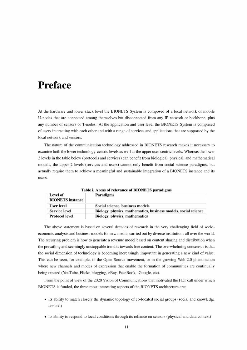
Table i. Areas of relevance of BIONETS paradigmsLevel of ParadigmsBIONETS instanceUser level Social science, business modelsService level Biology, physics, mathematics, business models, social scienceProtocol level Biology, physics, mathematics
The above statement is based on several decades of research in the very challenging field of socio-
economic analysis and business models for new media, carried out by diverse institutions all over the world.
The recurring problem is how to generate a revenue model based on content sharing and distribution when
the prevailing and seemingly unstoppable trend is towards free content. The overwhelming consensus is that
the social dimension of technology is becoming increasingly important in generating a new kind of value.
This can be seen, for example, in the Open Source movement, or in the growing Web 2.0 phenomenon
where new channels and modes of expression that enable the formation of communities are continually
being created (YouTube, Flickr, blogging, eBay, FaceBook, iGoogle, etc).
From the point of view of the 2020 Vision of Communications that motivated the FET call under which
BIONETS is funded, the three most interesting aspects of the BIONETS architecture are:
• its ability to match closely the dynamic topology of co-located social groups (social and knowledge
context)
• its ability to respond to local conditions through its reliance on sensors (physical and data context)
11

November 5, 2008 D2.1.1 Survey on paradigms BIONETS//wp2.1/0.1
• the long-term memory function that the sensors can support, which is similar to the pheronome trails
of an ant colony and that affords the system with something equivalent to a distributed, sub-symbolic
intelligence.
Clearly the architecture of the network is only one part of the story. What is needed is also a flexible,
dynamic, and adaptive service architecture that is able to keep up with the behaviour of the users and to meet
their changing service needs. This is where BIONETS is investing a great deal of effort in a biologically-
inspired approach that aims to endow the services and the underlying protocols with the ability to evolve.
Evolution, however, is only the tip of the iceberg: several additional paradigms from physics and biology
are being examined and are summarised and contextualised in Parts 1 and 2 of this report in order to meet
the challenging performance and adaptation requirements of a Bionet.
Performance optimisation and adaptability are therefore necessary to the realisation of the BIONETS
vision. However, they are not sufficient. The realisation of the 2020 Vision of Communications necessitates
an in-depth understanding of the needs and behaviour of the users if we want to develop an economi-
cally sustainable model of BIONETS-style communications. This is why Social Science is important in
BIONETS. In other words, social science can help us understand what BIONETS applications should adapt
to, thereby contributing to the definition of an appropriate fitness function.
The purpose and context for this work is best understood by realising that the integration of the models
examined and developed in this collection of articles is not meant to produce a unified body of theory. By
design, the research upon which this book is based is meant to look at different paradigms from a range of
different disciplines (mainly biology, physics, mathematics, and social science). These paradigms will then
be mapped to different parts of the project in the research that continues.
E Altman, P Dini, D Miorandi, D Schreckling
Public 12
Chapter 1
Introduction
This document is the fruit of the collection of paradigms and foundations that had been identified as being
relevant to the design, analysis and optimization of autonomous wireless networks, in general, and to the
Bionets architecture and services, in particular. The document contains three parts: paradigms from biology,
from physics and from social science. To summarize the motivation of studying these paradigms, we cite
Kelly (1991) [1]:
"There is currently considerable interest in the similarities between complex systems from diverse areas
of physics, economics and biology, and it is clear that the study of topics such as noisy optimization and
adaptive learning provide mathematical metaphors of value across many fields".
We describe below the various chapters, highlighting the specific contribution of the Bionets project to
the foundations and paradigms surveyed as well as the applicability to Bionets architecture and services.
1.1 Biologically inspired paradigms.
Machine Learning and control under uncertainty. Stochastic search algorithms have been widely re-
searched and used in the past decades for solving complex optimization problems. The paradigm advocates
the integration of machine learning techniques into stochastic search heuristics. In this chapter we provide
the main motivations leading to this paradigm, followed by a survey on the application of machine learning
to several types of stochastic search methods. The description of some recent work on this topic completes
the chapter.
Evolutionary games Evolutionary games provide a theoretical framework to understand and predict the
evolution of services, of protocols and of the architecture of decentralized networks whenever they evolve
in a competitive context. By a competitive environment we mean that evolution occurs among several
populations as a result of a process in which each population tries to improve its own fitness. Evolutionary
games have been introduced by biologists to explain and predict evolution. This paradigm has the potential
of further development when applied to engineering as rules of evolution of protocols, architecture and
services can be engineered so as to achieve desired stability and efficiency objectives. In our survey we first
present the basic bricks of evolutionary games, and then provide various applications of the evolution of
transport and of MAC layer protocols over wireless networks.
On Abstract Algebra and Logic: Towards their Application to Cell Biology and Security The material
13
November 5, 2008 D2.1.1 Survey on paradigms BIONETS//wp2.1/0.1
in this chapter is of an introductory nature, and is meant specifically to make some of the very abstract
ideas of algebra and logic more accessible to researchers from other or more applied disciplines. Algebra
and logic are very closely related. As a consequence a bridge to translate the regularities in cell structure
and behaviour into logic specifications of autonomic behaviour in services and protocols begins to appear
possible. In addition to introductory material the article also provides recent references that support this
perspective. The main areas of application within BIONETS for this work is in gene expression-based
computing and security.
Evolutionary Computing and Artificial Embryogeny In this chapter the authors present a review of
state-of-the-art techniques for automated creation and evolution of software. The focus is on bio-inspired
bottom-up approaches, in which complexity is grown from interactions among simpler units. First, the
authors review Evolutionary Computing (EC) techniques, highlighting their potential application to the
automated optimization of computer programs in an online, dynamic environment. Then, they survey
approaches inspired by embryology, in which artificial entities undergo a developmental process. The
chapter concludes with a critical discussion and outlook for applications of the aforementioned techniques
to the BIONETS environment.
Message Diffusion Protocols in Mobile Ad Hoc Networks The chapter surveys routing protocols in
mobile sparse ad-hoc networks. Due to low connectivity, direct paths do not exist between a source and
a destination, and end-to-end communication has to rely on mobility of terminals which relay packets.
Tools from epidemiology have been used to analyze the process of spreading of copies of the packets in the
network as well as mechanisms to stop it once the destination receives the packet.
1.2 Paradigms Related to Physics.
Various paradigms that we describe in this survey allow one to obtain macroscopic properties of a sys-
tem from the knowledge of the nature of microscopic interactions between basic elements of the system.
Applications to dense networks are discussed.
Scale-free networks. Scale-free distributions are known to appear often in various phenomena arising in the
natural world. From the BIONETS networking point of view, two cases of scale-free distribution have been
identified and studied. The first one deals with the scale-free structure arising in organisational networks
(usually expressed in terms of degree distribution of a graph representing the system’s relationships). This
has been proven to arise in a variety of systems, from social networks to the Internet and metabolic networks
The second one is concerned with the spatial distribution of nodes location in a network, which gives
rise, in various cases, to fractal-like behaviour. The survey reviews methods and tools for characterizing
and analyzing such cases, providing a useful model for (i) analyzing various issues related to BIONETS
disappearing networks (ii) providing a set of conditions for the arising of such structures, which are known
to show peculiar properties (robust yet fragile).
Spatial models from Optics, Electrostatics and Road traffic. Spatial models from electrostatics and
optics have been used for describing the paths followed by packets routed in dense ad-hoc network in a
context in which mobiles are connected (in contrast with the approaches described in Chapter 6 that are
suitable for disconnected networks). The limit as the density of the network becomes large can therefore be
Public 14
November 5, 2008 D2.1.1 Survey on paradigms BIONETS//wp2.1/0.1
described and its performance computed from simpler continuum models. We survey these approaches and
propose alternative ones based on tools from road traffic engineering.
Random Matrix Theory and free probability In many applications of wireless communications, we en-
counter matrices whose entries are random. Examples are gain matrices appearing in MIMO channels
which can be used for capacity calculations. In many cases, the distribution of the eigenvalues of the ma-
trices converge to some non-random limit as the number of entries in the matrices grow. The Theory of
random matrices allows us to derive explicit expressions for those limits and thus provide a powerful tool
for computing performance measures of systems with a large number of mobiles. This approach is based in
part on a recent theory called Free Probability which is surveyed as well.
1.3 Paradigms from Social Sciences.
Historical-Interpretive Considerations about Money as a Unit of Value and Scale-Dependent Phe-nomenon This chapter reviews the main concepts and theories about money as a medium of exchange and
economic models based on sharing of unused capital in the BIONETS environment. The rise of mobile
technology and the multiple applications and services that can be provided directly to users offer the op-
portunity to leverage the economics of sharing and community currencies to create a wider user base where
exchanges are economically motivated. Ubiquitous technology such as mobile devices raises new possible
applications in a virtual world to understand, apply and negotiate these concepts. T-Node/U-Node separa-
tion, evolving applications, inherent user feedback, etc. promise to represent a wider technology platform
providing more—and built-in—support for sharing and community currencies as the basis of new business
models at the intersection between business services and social networking.
Distributed approaches to graph based reputation measures Reputation systems are indispensable for
the operation of Internet mediated services, electronic markets, document ranking systems, P2P networks
and Ad Hoc networks. Here we survey available distributed approaches to the graph based reputation
measures. Graph based reputation measures can be viewed as random walks on directed weighted graphs
whose edges represent interactions among peers. We classify the distributed approaches to graph based
reputation measures into three categories. The first category is based on asynchronous methods. The
second category is based on the aggregation/decomposition methods. And the third category is based on
the personalization methods which use local information.
Network formation games Network structure plays an important role in the performance of distributed
systems, be it a group of friends, the World Wide Web or a business and commerce system. Researchers
from various fields like physics, economics and social sciences have therefore been studying network forma-
tion. In current Internet the network structure arises from interactions of agents at different levels. Internet
Service Providers (ISPs) and different organizations decide autonomously which other entities in the Inter-
net they want to be directly connected to. More recently Peer-to-Peer (P2P) networks and ad hoc networks
have introduced new actors shaping the current Internet structure. All these agents (ISPs, peers,...) may
have disjoint and competing interests, so game theory can provide useful mathematical tools to study the
outcomes of their interactions. In particular there is a growing research trend on so-called network forma-
tion games, which explicitly consider players who can decide to connect to each other. In these games the
network structure both influences the result of the economic interactions and is shaped by the decisions of
Public 15

November 5, 2008 D2.1.1 Survey on paradigms BIONETS//wp2.1/0.1
the players. The purpose of this chapter is to provide the reader unfamiliar with this research area with the
basic concepts, pointers to other surveys, and an overview of current results in the computer networks field.
Public 16

Bibliography
[1] F. P. Kelly, "Network Routing", Philosopical Transactions of the Royal Society, A337, 343–367, 1991.
[2] T. Tanaka, "Statistical mechanics of CDMA multiuser demodulation", Europhysics Letters, 54(4), pp.
540-546, 2001.
17

November 5, 2008 D2.1.1 Survey on paradigms BIONETS//wp2.1/0.1
Public 18

Part I
Biological Inspired Paradigms
19

Chapter 2
Machine Learning for IntelligentOptimizationM. Brunato
Abstract. Stochastic optimization algorithms have been widely researched and used in the past decades
for solving complex optimization problems. However, all such techniques require a lengthy phase of pa-
rameter tuning before being effective towards a particular problem; the tuning phase is performed by a
researcher who modifies the algorithm’s operating conditions according to his observations, therefore act-
ing as a learning component. The Reactive Search paradigm aims at integrating sub-symbolic machine
learning techniques into stochastic search heuristics, in order to automate the parameter tuning phase and
make it an integral part of the algorithm execution, rather than a pre-processing phase.
The self-regulation property envisioned by the Reactive Search concept is motivated by the observation
that in nature, and in particular in biological systems, feedback loops tend to be adaptive, i.e., they possess
a learning component. In this chapter we provide the main ideas leading to the Reactive Search paradigm,
followed by a survey on the application of Reactive Search concepts to several types of stochastic search
methods.
2.1 Introduction
Optimization heuristics are motivated by the widespread belief that most interesting problems cannot be
solved exactly within an acceptable time (e.g., time that is a low-degree polynomial function of the problem
size). The last forty years have seen the introduction of many problem-specific methods: notable early
examples are the Kernighan-Lin method for the graph partitioning problem [37] or the Steiglitz-Weiner
heuristic for the Traveling Salesman Problem [58]. Ideas from such methods have been successfully ex-
tracted and applied to more general techniques, therefore called meta-heuristics, aimed at tackling problems
in different domains by exploiting their similarity from a problem-solving viewpoint.
On the other hand, meta-heuristics suffer from the presence of operating parameters whose optimal
values depend on the problem and on the particular instance being solved. All such techniques require
therefore a (possibly long) phase of parameter tuning before being effective towards a particular problem,
21
November 5, 2008 D2.1.1 Survey on paradigms BIONETS//wp2.1/0.1
and in general the tuning phase is performed by a researcher who modifies the algorithm’s operating con-
ditions according to his observations, therefore acting as a learning component providing feedback to the
algorithm itself. The Reactive Search paradigm advocates the integration of sub-symbolic machine learn-
ing techniques into stochastic search heuristics, in order to automate the parameter tuning phase, therefore
making it an integral part of the algorithm execution, rather than an unaccounted preprocessing phase.
This chapter is organized as follows. Sec. 2.2 defines the application domain of optimization meta-
heuristics. Sec. 2.3 provides a review of the basic meta-heuristic techniques. Sec. 2.4 introduces the frame-
work of reactive search and presents a survey of recent developments. Applications of such techniques
are explored in Sec. 2.5. Finally, Sec. 2.6 discusses the relevance of the proposed techniques within the
BIONETS project.
2.2 Optimization problems
Throughout this chapter, a system will be described by a mathematical model whose parameter set (rep-
resenting its degrees of freedom) is given by its configuration space X ; an element X ∈ X , representing
a particular state of the system, is called a configuration. The criterion for measuring a configuration’s
fitness is defined within an objective function f : X →R. In some cases, the criterion formulation naturally
leads to a penalty measure, so that lower values of f (X) correspond to a better configuration, sometimes
the function will represent a fitness measure. The aim of optimization is to find a configuration X ∈ X that
minimizes f (X) (if it represents a penalty measure) or maximizes it (if it represents fitness). A problem
that can be expressed by the pair (X , f ) is called an optimization problem. If the configuration space Xis described in an implicit form by a system of equations and inequalities, then the problem is said to be
constrained, otherwise it is said to be unconstrained.
This chapter considers unconstrained optimization problems where configurations can be mixed tuples
of binary, integer or real values; the only form of constraints accepted in this context are the definition
intervals of the scalar components, and X can be expressed as a set product of intervals. While constrained
problems are a superclass of unconstrained ones (the latter being the limit case with zero constraints), a
constrained problem can always be transformed into an unconstrained one by accounting for constraint
violations as penalties in the objective function. However, the constrained formulation can benefit from
specific techniques, either analytical (e.g., Lagrange multipliers) or iterative (e.g., the simplex method and
its many extensions), so that such reduction may decrease the chance of finding good solutions.
As a fundamental unconstrained example, let us consider the Maximum Satisfiability (MAXSAT) prob-
lem (see [25] for a classical survey), where n Boolean variables x1, . . . ,xn are given. An atom is defined as
either a variable xi or the negation of a variable xi, and a (disjunctive) clause is the disjunction (logical OR)
of a finite set of atoms. Given a finite set S of clauses, we ask what is the truth assignment to the n variables
that maximizes the number of true clauses in S. In this case, the configuration space is X = 0,1n (all
possible truth assignments), while the objective function is
f (X) = ∑c∈S
χc(X),
where χc(X) is 1 if the truth assignment X satisfies the clause c, 0 otherwise.
Public 22
November 5, 2008 D2.1.1 Survey on paradigms BIONETS//wp2.1/0.1
MAXSAT is still a very active research subject, and it is a useful benchmark for many techniques. Some
are specifically aimed at characteristics of that domain; for instance, the AdaptNovelty+ heuristic [59],
although based on heuristics that span many applications, exploits peculiarities of the MAXSAT problem.
On the other hand, the last 40 years have seen the introduction of many heuristic methods that are
applicable to different problems. We can define a meta-heuristic as a class of methods, operating on different
domains, all sharing the same basic principle. Ideally, a meta-heuristic operates by receiving as input the
pair (X , f ) describing the problem, and outputs an element X ∈ X selected in order to optimize f . Note
that in this formulation the heuristic has no clue about the particular problem it is asked to solve; all such
information has been used by the researcher to build the configuration space X and the objective function
f , which is treated as a “black box” by the algorithm.
Research work in this area was motivated by the observation that, when expressed in terms of fitness-
function optimization, the properties of many problems can be described in terms of a common framework,
which will be detailed in Sec. 2.2.1–2.2.2.
2.2.1 Neighborhood structure
Very often, the problem that we are solving has a “canonical” topological structure defining when two
configurations of the same instance may be considered “close” to each other. Considering such structure
often carries advantages in the optimization process. Two configurations of a MAXSAT instance may differ
by the value of a single variable. In this case, we naturally consider such configurations to be “similar,” and
we expect most clauses (all clauses that do not contain the modified variable) to maintain the same truth
value. The most common way of defining a topology on a configuration set is by defining a neighborhood
for every configuration. Consider the MAXSAT case: given a configuration X ∈ X , let its neighborhood be
defined as all configurations that differ from it by at most one bit:
N(X) = X ′ ∈ X |H(X ,X ′)≤ 1,
where H(·, ·) is the Hamming distance between two configurations, i.e., the number of bits by which they
differ. A neighborhood topology on X is therefore the set
N = (X ,N(X))|X ∈ X .
An immediate advantage of considering this neighborhood relationship between configurations is that, if
the objective function is described by appropriate data structures, its value can be computed incrementally,
saving CPU time.
A second, more important advantage of maintaining a neighborhood relationship between configura-
tions is that nearby solutions tend to have similar properties, so that if a configuration is “good” with
respect to the objective function then its surroundings are worth exploring. In other words, once a topol-
ogy N is imposed upon a configuration space X , the objective function can be expected to manifest some
form of “regularity” with respect to it. In particular, the triplet (X ,N , f ) can be analyzed in terms of a
landscape [35, 60] in order to study the dynamics of solving algorithms on particular problems.
Looking in the proximity of known solutions is known as intensification of the search process (see [55]
for an analysis) or exploitation of the solution. Stochastic local search techniques [31] aim at implementing
Public 23

November 5, 2008 D2.1.1 Survey on paradigms BIONETS//wp2.1/0.1
X (input) Search space descriptionN (input) Neighborhood structuref (input) Objective functiont (local) Iteration counter
X (t) (local) Current configuration at iteration tX (local) Best configuration found so far
1. function LocalSearch (X , N , f )2. t ← 03. X (0) ← choose an element in X4. X ← X (0)
5. while some continuation condition is satisfied6. t ← t +17. X (t) ← choose an element in N(X (t−1))8. if f (X (t)) > f (X)9. X ← X (t)
10. end if11. end while12. return X13. end function
Figure 2.1: The basic Local Search framework: the algorithm moves between neighboring configurations
this principle. The basic structure of a local search algorithm is shown in Fig. 2.1: the algorithm repeatedly
moves from a configuration to a neighboring one (the loop in lines 2.2.1–2.2.1), storing the best configura-
tion found so far (lines 2.2.1–2.2.1). Heuristics differ in the choice of the initial configuration (line 2.2.1 of
Fig. 2.1), of the subsequent neighbors (line 2.2.1), and the continuation condition (line 2.2.1).
2.2.2 Large-scale structure
In the previous section we have seen how a local search optimization algorithm can move between neigh-
boring configurations with the goal of improving the objective function by means of incremental changes.
Unfortunately, trying to improve the current solution by only performing incremental steps causes much
of the problem’s search space to remain unexplored. Moreover, if the choice of the new configuration is
always done towards the improvement of the objective function value, the system will finally get stuck
in a locally optimal set of configurations. Note that optimization heuristics can be modeled as dynamic
systems [29], describing their structure in terms of attractors (local optima) and attraction basins (sets of
initial configurations leading to the same local optimum).
Once a local optimum has been achieved, further intensification of search in its neighborhood becomes
clearly counterproductive. Therefore, a diversification, or exploration strategy is needed. For example,
restarting from a new random configuration, in the hope to reach for a new portion of the search space,
can be a good policy. However, in many practical cases the distribution of local optima should be taken
into account: rather than restarting elsewhere, the algorithm should make an effort into trying to exit the
current basin of attraction by executing local moves. In the context of local search meta-heuristics, this can
be achieved in many ways, each leading to a broad class of heuristics.
Heuristics that do not base their behavior on the local search paradigm (e.g., population-based or model-
based algorithms) do not suffer from such local optimum entrapment; they will also be covered in Sec. 2.3.
Public 24
November 5, 2008 D2.1.1 Survey on paradigms BIONETS//wp2.1/0.1
Figure 2.2: Variable neighborhood search: the used neighborhood (bold circle around the current configu-ration) varies along the search trajectory.
2.3 Basic optimization meta-heuristics
In this section we briefly summarize and review the basic groups of meta-heuristic algorithms for optimiza-
tion. These heuristics differ both in the method chosen for intensification (some are based on local search,
others implement mutation operators) and diversification.
2.3.1 Variable Neighborhood Search
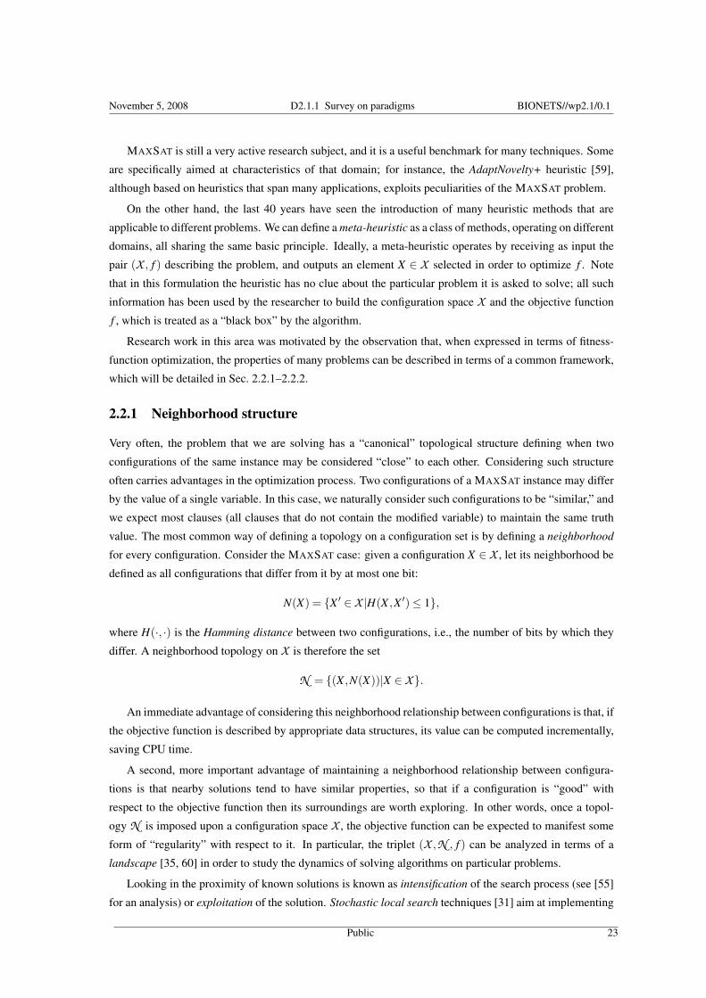
A problem formulation may allow for different neighborhood definitions, each inducing a different topology
on the search space. Moreover, there are cases when no optimal and fixed neighborhood is defined for a
problem because of lack of information. In many cases, however, adaptation of the neighborhood to the
local configuration is beneficial.
The seminal idea of the Variable Neighborhood Search (VNS) technique [24] is to consider a set of
predefined neighborhoods, and aim at using the most appropriate one during the search, as illustrated in
Fig. 2.2, where the possible neighborhoods are represented as concentric circles around configurations, and
the selected one is bold.
Many schemes for using the set of different neighborhoods in an organized way are possible [27].
Variable Neighborhood Descent (VND) uses a default neighborhood first; other neighborhoods are ranked
in some order of importance and are used only if the default neighborhood fails (i.e., the current point is
a local minimum for it), and only until an improving move is identified, after which the algorithm reverts
back to the default. If the ordering of the neighborhoods is related to the strength of the perturbation,
the algorithm will always use the minimum perturbation leading to an improvement. Variants of VND
include REDUCED-VNS [44], a stochastic version where only one random neighbor is generated before
deciding about moving or not, and SKEWED-VNS [26], where worsening moves are accepted if they lead
the search trajectory sufficiently far from the current point. Other versions of VNS employ a stochastic
move acceptance criterion, in the spirit of Simulated Annealing (see Sec. 2.3.2) as implemented in the
large-step Markov-chain version described in [41, 40], where “kicks” of appropriate strength are used to
exit from local minima.
Public 25
November 5, 2008 D2.1.1 Survey on paradigms BIONETS//wp2.1/0.1
2.3.2 Simulated annealing
The Simulated Annealing (SA) local search heuristic (see [38] for the seminal idea) introduces a tempera-
ture parameter T which determines the probability that worsening moves are accepted: a larger T implies
that more worsening moves tend to be accepted, therefore diversification becomes larger. This behavior is
obtained by implementing variants of the following move acceptance rule, where X (t) is the configuration
(solution) at iteration t and X ′ is a randomly chosen neighbor:
X ′ ← random element in N(X (t))
X (t+1) ←
X ′ if f (X ′)≤ f (X (t))
X ′ with probability p = e−f (X ′)− f (X(t))
T if f (X ′) > f (X (t))X (t) otherwise.
(2.1)
Simulated Annealing has the properties of a Markov memoryless process: waiting long enough, every
dependency on the initial configuration is lost, and the probability of finding a given configuration at a
given state will be stationary and only dependent on the value of f . If T goes to zero the probability will
peak only at the globally optimal configurations. This basic result raised high hopes of solving optimization
problems through a simple and general-purpose method, starting from seminal work in physics [43] and in
optimization [52, 15, 38, 1].
Note that the dynamics of the Simulated Annealing heuristic depend on the value of T . If T = 0, only
non-worsening paths are generated, leading to a local optima without any possibility of escape; if T = ∞,
all moves are equally probable, leading to a random walk in the configuration space. The basic mechanism
is a progressive reduction of T . The rate of reduction is called the annealing (or cooling) schedule, and
many such schedules have been analyzed for different problems [2, 16, 17].
2.3.3 Prohibition-based (Tabu) Search
The Tabu Search (TS) meta-heuristic [22] is based on the use of prohibitions as a complement to basic
heuristic algorithms like local search, with the purpose of guiding the basic heuristic beyond local optimal-
ity.
Let us assume, for instance, that the configuration space is the set of binary strings with a given length
n: X = 0,1n. Given the current configuration X (t), in Tabu Search only a subset NA(X (t)) ⊂ N(X (t)) of
neighbors is allowed, while the other neighbors are prohibited. The general way of generating the search
trajectory that we consider is given by:
X (t+1) = BESTNEIGHBOR(NA(X (t)))
NA(X (t+1)) = N(X (t+1))∩ALLOW(X (0), ...,X (t+1))
The set-valued function ALLOW selects a subset of N(X (t+1)) in a manner that in the general case depends
on the entire past trajectory X (0), ...,X (t+1). In practice, only a part of the search history is considered: for
instance, a prohibition period T can be defined such that the ALLOW function only takes into consideration
the T previous steps.
Public 26
November 5, 2008 D2.1.1 Survey on paradigms BIONETS//wp2.1/0.1
H = 8
0
0
0
0
0
0
0
0
0
1
1
1
1
1
1
1
1
1
1
1
1
0
0
0
0
0
0
1
1
1
1
1
0
0
0
0
0
0
0
Initial bit string
H = 1
H = 2
H = 3
H = 4
H = 5
H = 6
H = 7
H = 7
0
1 1 1 1 1 1 1 1 1 1 10 0 0 0 0 0 0 0 0 0 0 0
1 1 1 1 1 1 1 1 1 10 0 0 0 0 0 0 0 0 0 0 0
1 1 1 1 1 1 1 1 1 10 0 0 0 0 0 0 0 0 0 0
1 1 1 1 1 1 1 1 10 0 0 0 0 0 0 0 0 0 0
1 1 1 1 1 1 1 10 0 0 0 0 0 0 0 0 0 0
1 1 1 1 1 1 10 0 0 0 0 0 0 0 0 0 0
1 1 1 1 1 1 10 0 0 0 0 0 0 0 0 0
0 1 1 1 1 1 1 10 0 0 0 0 0 0 0 0
0 1 1 1 1 1 1 10 0 0 0 0 0 0 0
1 1 1 1 1 1 1 10 0 0 0 0 0 0 0
0
Selected for change Frozen
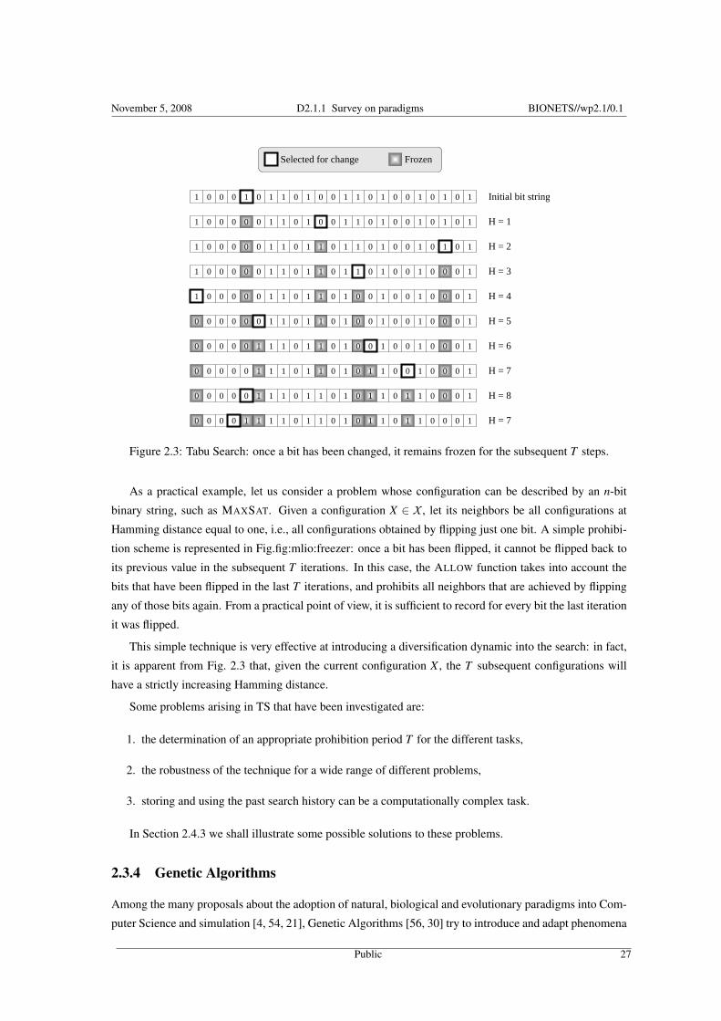
Figure 2.3: Tabu Search: once a bit has been changed, it remains frozen for the subsequent T steps.
As a practical example, let us consider a problem whose configuration can be described by an n-bit
binary string, such as MAXSAT. Given a configuration X ∈ X , let its neighbors be all configurations at
Hamming distance equal to one, i.e., all configurations obtained by flipping just one bit. A simple prohibi-
tion scheme is represented in Fig.fig:mlio:freezer: once a bit has been flipped, it cannot be flipped back to
its previous value in the subsequent T iterations. In this case, the ALLOW function takes into account the
bits that have been flipped in the last T iterations, and prohibits all neighbors that are achieved by flipping
any of those bits again. From a practical point of view, it is sufficient to record for every bit the last iteration
it was flipped.
This simple technique is very effective at introducing a diversification dynamic into the search: in fact,
it is apparent from Fig. 2.3 that, given the current configuration X , the T subsequent configurations will
have a strictly increasing Hamming distance.
Some problems arising in TS that have been investigated are:
1. the determination of an appropriate prohibition period T for the different tasks,
2. the robustness of the technique for a wide range of different problems,
3. storing and using the past search history can be a computationally complex task.
In Section 2.4.3 we shall illustrate some possible solutions to these problems.
2.3.4 Genetic Algorithms
Among the many proposals about the adoption of natural, biological and evolutionary paradigms into Com-
puter Science and simulation [4, 54, 21], Genetic Algorithms [56, 30] try to introduce and adapt phenomena
Public 27

November 5, 2008 D2.1.1 Survey on paradigms BIONETS//wp2.1/0.1
X (input) Search space descriptionf (input) Objective functionP (local) Current populationP ′ (local) Temporary population under construction
1. function GeneticOptimization (X , f )2. P ← choose elements from X3. while some continuation condition is satisfied4. Compute f (X) for each X ∈ P5. P ′← SELECT(P , f )6. for selected pairs X ,Y ∈ P ′7. P ′← P ′∪COMBINE(X ,Y )8. end for9. for random individuals X ∈ P ′
10. X ← MUTATE(X)11. end for12. P ← P ′13. end while14. return best configuration ever visited15. end function
Figure 2.4: The basic Genetic Algorithm framework: the algorithm maintains a population of individualsthat undergo selection, mutation and cross-combination. Standard bookkeeping operations such as optimummaintenance are not shown.
found in the natural framework of Evolution within the family of optimization techniques, placing them-
selves within the broader context of Evolutionary Computation (see also Chapter 5),
Evolutionary concepts are usually translated in the following way. An individual is a candidate solution
and its genetic content (genotype) corresponds to its configuration X ∈ X . A population is a set of indi-
viduals. The genotype of an individual is randomly changed by mutations (changes in X). The suitability
of an individual with respect to the environment is described by the fitness function f . Finally, fitter in-
dividuals are allowed to produce a larger offspring (new candidate solutions), whose genetic material is a
recombination of the genetic material of their parents.
As shown in Fig. 2.4, the basic GA maintains a population P ⊂ X and makes it undergo a sequence of
modifications produced by operators. The main types of operators are:
• SELECT: given a population P ⊆ X , produces a subset P ′ ⊆ P according to the fitness of individuals
and to stochastic factors. Usually, the value of the objective function for a given individual X ∈ P is
used to determine the probability of its survival.
• MUTATE: given an individual X ∈ X , produces a new individual X ′ by applying transformations
consisting of pointwise changes, substring swappings or other mechanisms, depending both on the
structure of the configuration space and the natural mechanism that is being emulated.
• COMBINE: given two individuals X ,Y ∈ X , a new individual Z is generated by combining parts of
the genotype of X and Y . In the simplest case, every component of Z is chosen randomly from X or
Y (uniform cross-over).
After the generation of an initial population P (line 2.3.4 of Fig. 2.4), the algorithm iterates through a
Public 28

November 5, 2008 D2.1.1 Survey on paradigms BIONETS//wp2.1/0.1
sequence of basic operations: the fitness of each individual is computed, then some individuals are chosen
by a random selection process that favors elements with a high fitness function (line 2.3.4); a cross-over
combination is applied to randomly selected survivors in order to combine their features (lines 2.3.4–2.3.4),
then some individuals undergo a random mutation (lines 2.3.4–2.3.4). The algorithm is then repeated on
the new population.
For example, in an optimization problem where the configuration is described by a binary string, such
as MAXSAT, mutation may consist of randomly changing bit values with a fixed small probability and
recombination of string X and Y may consist of building a new string Z so that
∀i = 1, . . . ,n Zi =
Xi with probability 1/2Yi with probability 1/2.
Many hybridizations between Genetic Algorithms and Local Search algorithms have been proposed.
The term memetic algorithms [45, 39] has been introduced for models which combine the evolutionary
adaptation of a population with individual learning within the lifetime of its members. The term derives
from Dawkins’ concept of a meme which is a unit of cultural evolution that can exhibit local refinement [18].
In these techniques, a team member can execute a more directed and determined exploitation of its initial
genetic content (its initial position). This is effected by considering the initial genotype as a starting point
and by initiating a run of local search from this initial point, for example scouting for a local optimum.
There are two ways in which such individual learning can be integrated: a first way consists of replacing
the initial genotype with the better solution identified by local search (leading to a sort of Lamarckian
evolution, where the parent transmits its own experience through its genes); a second way can be that of
maintaining the original genotype, but modifying the individual’s fitness by taking into account not the
initial value but the final one obtained through local search. In other words, the fitness does not evaluate
the initial state but the value of the “learning potential” of an individual, measured by the result obtained
after the local search. These forms of combinations of learning and evolution are known as the Baldwin
effect [28, 61], and have the effect of changing the fitness landscape, while the resulting form of evolution
is still Darwinian in nature.
2.3.5 Model-based heuristics
The main idea of model-based optimization is to create and maintain a model of the problem, whose aim is to
provide some clues about the problem’s solutions. If the problem is a function to be minimized, for instance,
it is helpful to think of such model as a simplified version of the function itself, or a probability distribution
defining the estimated likelihood of finding a good quality solution at a certain point. When used to optimize
functions of continuous variables, model-based optimization is related to surrogate optimization, where a
surrogate function is used to generate new sample points instead of the original function, which is in some
cases very costly to compute, see for example [34], and also connected to the kriging [42] and response
surface methodologies [47].
To solve a problem, the model is used to generate a candidate solution, which is in turn checked. The
result of the check is used to refine the model, so that the future generation is biased towards better candidate
solutions. Clearly, for a model to be useful it must provide as much information about the problem as
Public 29
November 5, 2008 D2.1.1 Survey on paradigms BIONETS//wp2.1/0.1
Unknown optimum
O
Function
1
2
model
model
Sampled points
x
f(x)
e a b c d
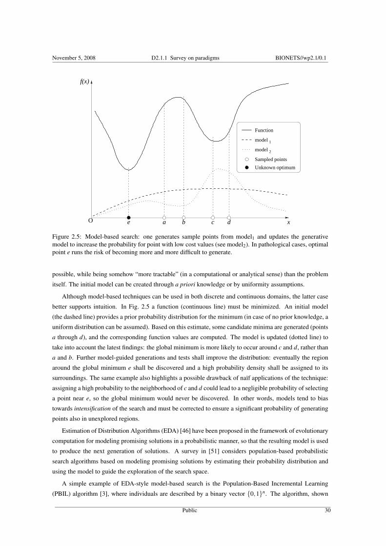
Figure 2.5: Model-based search: one generates sample points from model1 and updates the generativemodel to increase the probability for point with low cost values (see model2). In pathological cases, optimalpoint e runs the risk of becoming more and more difficult to generate.
possible, while being somehow “more tractable” (in a computational or analytical sense) than the problem
itself. The initial model can be created through a priori knowledge or by uniformity assumptions.
Although model-based techniques can be used in both discrete and continuous domains, the latter case
better supports intuition. In Fig. 2.5 a function (continuous line) must be minimized. An initial model
(the dashed line) provides a prior probability distribution for the minimum (in case of no prior knowledge, a
uniform distribution can be assumed). Based on this estimate, some candidate minima are generated (points
a through d), and the corresponding function values are computed. The model is updated (dotted line) to
take into account the latest findings: the global minimum is more likely to occur around c and d, rather than
a and b. Further model-guided generations and tests shall improve the distribution: eventually the region
around the global minimum e shall be discovered and a high probability density shall be assigned to its
surroundings. The same example also highlights a possible drawback of naïf applications of the technique:
assigning a high probability to the neighborhood of c and d could lead to a negligible probability of selecting
a point near e, so the global minimum would never be discovered. In other words, models tend to bias
towards intensification of the search and must be corrected to ensure a significant probability of generating
points also in unexplored regions.
Estimation of Distribution Algorithms (EDA) [46] have been proposed in the framework of evolutionary
computation for modeling promising solutions in a probabilistic manner, so that the resulting model is used
to produce the next generation of solutions. A survey in [51] considers population-based probabilistic
search algorithms based on modeling promising solutions by estimating their probability distribution and
using the model to guide the exploration of the search space.
A simple example of EDA-style model-based search is the Population-Based Incremental Learning
(PBIL) algorithm [3], where individuals are described by a binary vector 0,1n. The algorithm, shown
Public 30

November 5, 2008 D2.1.1 Survey on paradigms BIONETS//wp2.1/0.1
f (input) Objective functionL (input) Number of bits in the configuration stringρ (input) Learning ratep (local) Generative model probability vectorP (local) Current populationP ′ (local) Selected fittest populationX (local) Best configuration found so far
1. function PBIL ( f , L, ρ)2. p←0.5L
3. while some continuation condition is satisfied4. P ← sample set generated with vector p5. P ′← fittest solutions within P6. for each sample X ∈ P ′7. p← (1−ρ)p+ρX8. end for9. end while
10. return best configuration ever visited11. end function
Figure 2.6: Population-Based Incremental Learning: the algorithm updates a generative model by repeat-edly generating a population of solutions and selecting the best individuals. Standard bookkeeping opera-tions such as optimum maintenance are not shown.
in Fig. 2.6, maintains a probabilistic generative model with parameters p = (p1, . . . , pn) ∈ [0,1]n. This
model is used to generate a population of candidate solutions P (line 2.3.5). A selection of the fittest
solutions (line 2.3.5) is used to modify the probability estimates of the solution’s components, which are
incrementally updated by a moving average (lines 2.3.5–2.3.5).
Another algorithm in the EDA framework is Mutual-Information-Maximizing Input Clustering (MIMIC) [19].
Given a function f to minimize within configuration space X , the technique tries to set a convenient thresh-
old θ and to estimate the distribution pθ of solutions whose objective value is lower than θ. For selecting
the proper threshold (notice that if θ is too low, no point is considered, while if it is too high all points are),
the technique proposes a fixed percentile of a sampled subset. The algorithm then works by progressively
lowering the threshold, identifying the distribution of the fittest values. In order to compute the distribu-
tion within an acceptable CPU time, distributions are projected onto a reduced space by minimizing the
Kullback-Leibler divergence.
2.4 Reactive search concepts
This Section contains a review of the main ideas that underlie the Reactive Search principle, on the basis of
the common aspects listed in Sec. 2.2, and applied to the heuristics described in Sec. 2.3. More details can
be found in [9, 11].
The motivating observation for Reactive Search is the fact that all heuristics described up to now are
parametric. It is difficult to assess, or even define, the best value for these parameters, which depends on
the problem being addressed, on the particular instance, and on the aim of the researcher (do we want fast
convergence towards the global optimum, or to an acceptable suboptimal solution?). The need for parameter
tuning leads to a scenario where the (human) researcher adjusts the search algorithm’s parameters in order
Public 31
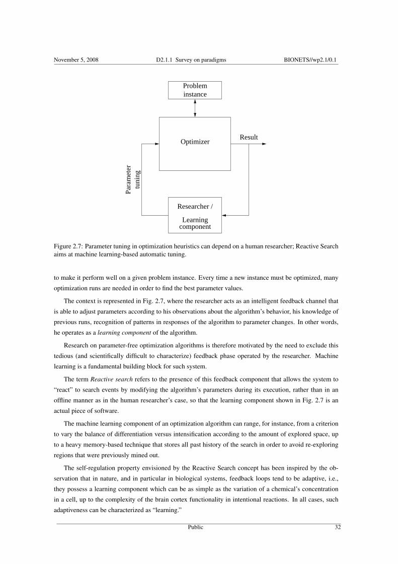
November 5, 2008 D2.1.1 Survey on paradigms BIONETS//wp2.1/0.1
Researcher /
Optimizer
Probleminstance
ResultPa
ram
eter
tuni
ng
componentLearning
Figure 2.7: Parameter tuning in optimization heuristics can depend on a human researcher; Reactive Searchaims at machine learning-based automatic tuning.
to make it perform well on a given problem instance. Every time a new instance must be optimized, many
optimization runs are needed in order to find the best parameter values.
The context is represented in Fig. 2.7, where the researcher acts as an intelligent feedback channel that
is able to adjust parameters according to his observations about the algorithm’s behavior, his knowledge of
previous runs, recognition of patterns in responses of the algorithm to parameter changes. In other words,
he operates as a learning component of the algorithm.
Research on parameter-free optimization algorithms is therefore motivated by the need to exclude this
tedious (and scientifically difficult to characterize) feedback phase operated by the researcher. Machine
learning is a fundamental building block for such system.
The term Reactive search refers to the presence of this feedback component that allows the system to
“react” to search events by modifying the algorithm’s parameters during its execution, rather than in an
offline manner as in the human researcher’s case, so that the learning component shown in Fig. 2.7 is an
actual piece of software.
The machine learning component of an optimization algorithm can range, for instance, from a criterion
to vary the balance of differentiation versus intensification according to the amount of explored space, up
to a heavy memory-based technique that stores all past history of the search in order to avoid re-exploring
regions that were previously mined out.
The self-regulation property envisioned by the Reactive Search concept has been inspired by the ob-
servation that in nature, and in particular in biological systems, feedback loops tend to be adaptive, i.e.,
they possess a learning component which can be as simple as the variation of a chemical’s concentration
in a cell, up to the complexity of the brain cortex functionality in intentional reactions. In all cases, such
adaptiveness can be characterized as “learning.”
Public 32
November 5, 2008 D2.1.1 Survey on paradigms BIONETS//wp2.1/0.1
The advantage in automated parameter tuning is twofold: it provides complete documentation on the
algorithm, which becomes self-contained and does not depend on external factors (i.e., human supervision),
and removes the fine-tuning work from the researcher.
Reactive techniques have been proposed within many different optimization frameworks. Most reactive
schemes are based on a common mechanism: first, the program maintains a history of the past search evolu-
tion. Next, this trace is used to identify local minimum entrapment situations (e.g., the same configurations
are repeatedly visited), to identify patterns in the distribution of local minima, to build probabilistic models.
Finally, the outcome of the learning process, which takes place along the execution of the search, is used
to modify the basic search parameters which, in the stochastic search context, usually control the balance
between intensification and diversification mechanisms.
In the following sections, applications of the Reactive Search concept to the basic optimization meta-
heuristics are surveyed.
2.4.1 Variable Neighborhood Search
An explicitly reactive VNS is considered in [12] for the Vehicle Routing problem with Time Windows
(VRPTW), where a construction heuristic is combined with VND using first-improvement local search.
The objective function used by the local search operators is modified to consider the waiting time to escape
from a local minimum. A preliminary investigation about a self-adaptive neighborhood ordering for VND
is presented in [32]. Ranking of the different neighborhoods depends on their observed benefits in the past
and is dynamically changed during the search.
2.4.2 Simulated annealing
On-line learning strategies can be introduced in the algorithm’s cooling schedule, by letting parameter T
vary according to the search results. A very simple proposal [17] suggests resetting the temperature once
and for all at a constant temperature high enough to escape local minima but also low enough to visit
them. For example, at the temperature Tfound when the best heuristic solution is found in a preliminary SA
simulation. The basic design principle is related to: i) exploiting an attraction basin rapidly by decreasing
the temperature so that the system can settle down close to the local minimizer, ii) increase the temperature
to diversify the solution and visit other attraction basins, iii) decrease again after reaching a different basin.
As usual, the temperature increase in this kind of non-monotonic cooling schedule has to be rapid enough to
avoid falling back to the current local minimizer, but not too rapid to avoid a random-walk situation (where
all random moves are accepted) which would not capitalize on the local structure of the problem.
Possibilities to increase the temperature to escape local optima include resetting the temperature to
Treset = Tfound, the temperature value when the current best solution was found [50]. Geometric re-heating
phases can be used [2], which multiply T by a heating factor γ larger than one at each iteration during a
reheat phase. Enhanced versions involve a learning process to choose a proper value of the heating factor
depending on the system state. In particular, γ is close to one at the beginning, while it increases if, after a
fixed number of escape trials, the system is still trapped in the local minimum.
Modifications departing from the exponential acceptance rule (2.1) and adaptive stochastic local search
methods for combinatorial optimization are considered in [48, 49], where the authors note that adaptations
Public 33
November 5, 2008 D2.1.1 Survey on paradigms BIONETS//wp2.1/0.1
should be done by the algorithm itself or by the user, by means of some learning mechanism. A simple
adaptive technique suggested in [49] is the SEQUENCEHEURISTIC: a perturbation leading to a worsening
solution is accepted if and only if a fixed number of trials could not find an improving perturbation (this
can be seen as deriving evidence of “entrapment” in a local minimum and activating reactively an escape
mechanism). In this way the temperature parameter is eliminated. The positive performance of the SE-
QUENCEHEURISTIC in the area of design automation suggests that the success of SA is “due largely to
its acceptance of bad perturbations to escape from local minima rather than to some mystical connection
between combinatorial problems and the annealing of metals” [49].
“Cybernetic” optimization is proposed in [20] as a way to use probabilistic information for feedback
during a run of SA. The idea is to consider more runs of SA running in parallel and to aim at intensifying
the search by lowering the temperature parameter when there is evidence that the search is converging to
the optimum value.
2.4.3 Tabu Search
In reactive versions of Tabu Search, most notably the Reactive Tabu Search (RTS) strategy [8], the prohibi-
tion period T is determined through feedback (i.e., reactive) mechanisms during the search. T is equal to one
at the beginning (meaning that the inverse of a given move is prohibited only at the next step), it increases
only when there is evidence that diversification is needed, it decreases when this evidence disappears. The
evidence that diversification is needed is signaled by the repetition of previously visited configurations. All
configurations found during the search can be stored in memory in a lazy learner fashion, or populate a more
complex data structure. After a move is executed the algorithm checks whether the current configuration
has already been found and it reacts accordingly (T increases if a configuration is repeated, T decreases if
no repetitions occurred during a sufficiently long period).
RTS can be characterized as a memory-based search strategy where efficient data structures are needed
to store and retrieve previously visited configurations in low amortized time. This can be obtained by
combining hash tables with persistent data structures such as red-black trees [6, 5].
2.4.4 Genetic and Population-based algorithms
In the Genetic Algorithms (GA) context, the concept of metalevel Genetic Algorithm [23] (meta-GA) has
been proposed. Here the problem instance is solved by a population of GAs whose genotype is represented
by their parameters. The fitness of these “individual” algorithms is measured by their performance in
solving the problem, and an overlying GA is used to select the best individuals.
In this case, the overlying GA implements the feedback loop that is characteristic of the Reactive Search
paradigm, see for example [57, 62] for applications.
2.5 Biology-inspired applications
In this section we present two examples of reactive search applied to biology-inspired scenarios. In the
first case (Section 2.5.1) we investigate a possible extension of a population-based approach by introducing
“intelligent” individuals that apply a low-knowledge reactive scheme for local search. In the second part
Public 34
November 5, 2008 D2.1.1 Survey on paradigms BIONETS//wp2.1/0.1
(Section 2.5.2) the distribution of local search algorithms on several machines is studied in terms of a
tradeoff between the rate of knowledge exchange (performed in an epidemic, peer-to-peer fashion) and the
quality of the solution found.
2.5.1 A population-based approach to reactive search
A clique is a complete graph. The Maximum Clique problem asks for finding the largest complete subgraph
embedded in a given graph. It is a well-known NP-hard problem: its decision version is NP-complete and
non-approximable. Therefore, it is a well-studied testing ground for combinatorial meta-heuristics, see for
instance the DIMACS competition benchmark [33].
Following the recent introduction of Evolutionary Algorithms with Guided mutation for solving the
maximum clique problem (EA/G [63]), the reactive and evolutionary algorithm R-EVO [10] has been pro-
posed in the framework of estimation-of-distribution algorithms (EDA).
Classical model-guided mutation schemes use a model distribution to generate the offspring by combin-
ing the local information of solutions found so far with global statistical information (since they are based
on a learning component, such algorithms, and in particular EA/G, can be considered within the reactive
search paradigm). The R-EVO algorithm is placed in the same evolutionary framework, but considers more
complex individuals, which modify tentative solutions by local search. In particular, the estimated distribu-
tion is used to periodically initialize the state of each individual based on the previous statistical knowledge
extracted from the population. Each individual in R-EVO adopts a drastically simplified low-knowledge
version of reactive local search (RLS) [7], with a simple internal diversification mechanism based on tabu-
search, and a prohibition parameter proportional to the estimated best clique size. R-EVO is competitive
with the more complex full-knowledge RLS-EVO which adopts the original RLS algorithm.
In [10] we study the combination of the EDA mechanism (which lies at the basis of thee EA/G al-
gorithm) with a stochastic local search algorithm derived from Reactive Tabu Search; we show that the
resulting technique produces significantly better results than EA/G for most of the benchmark instances
and is remarkably robust with respect to the setting of the algorithm parameters.
2.5.2 Gossiping Search Heuristics
While the use of distributed computing in search and optimization problems has a long research history,
most efforts have been devoted to parallel implementations with strict synchronization requirements or to
distributed architectures where a central server coordinates the work of clients by partitioning the search
space or working as a status repository.
The distributed realization of a global optimization algorithm ranges from independent execution of
instances (useful to mitigate very frequent heavy-tail behaviors) to complete synchronization and sharing
of information (e.g., processes in a shared-memory multiprocessor machine). Between these two extremal
cases, a wide spectrum of algorithms can be designed to perform individual searches with some form
of loose coordination. Some paradigmatic cases of “collaborative search” are now collected under the
BOINC initiative [53]. Although distributed, these projects are based on the repetition of a simple loop:
every involved machine receives from a central server a subset of the search space (signal samples, number
Public 35
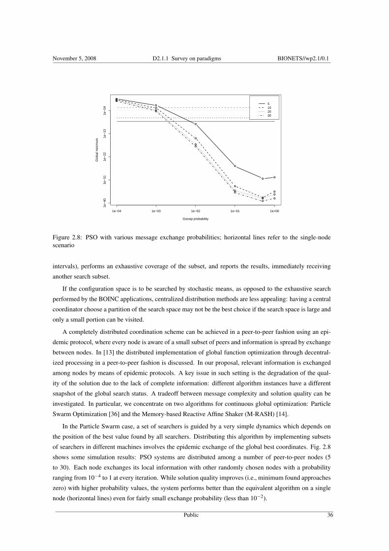
November 5, 2008 D2.1.1 Survey on paradigms BIONETS//wp2.1/0.1
1e−04 1e−03 1e−02 1e−01 1e+00
1e−
401e
−31
1e−
221e
−13
1e−
04
Gossip probability
Glo
bal m
inim
um
5102030
Figure 2.8: PSO with various message exchange probabilities; horizontal lines refer to the single-nodescenario
intervals), performs an exhaustive coverage of the subset, and reports the results, immediately receiving
another search subset.
If the configuration space is to be searched by stochastic means, as opposed to the exhaustive search
performed by the BOINC applications, centralized distribution methods are less appealing: having a central
coordinator choose a partition of the search space may not be the best choice if the search space is large and
only a small portion can be visited.
A completely distributed coordination scheme can be achieved in a peer-to-peer fashion using an epi-
demic protocol, where every node is aware of a small subset of peers and information is spread by exchange
between nodes. In [13] the distributed implementation of global function optimization through decentral-
ized processing in a peer-to-peer fashion is discussed. In our proposal, relevant information is exchanged
among nodes by means of epidemic protocols. A key issue in such setting is the degradation of the qual-
ity of the solution due to the lack of complete information: different algorithm instances have a different
snapshot of the global search status. A tradeoff between message complexity and solution quality can be
investigated. In particular, we concentrate on two algorithms for continuous global optimization: Particle
Swarm Optimization [36] and the Memory-based Reactive Affine Shaker (M-RASH) [14].
In the Particle Swarm case, a set of searchers is guided by a very simple dynamics which depends on
the position of the best value found by all searchers. Distributing this algorithm by implementing subsets
of searchers in different machines involves the epidemic exchange of the global best coordinates. Fig. 2.8
shows some simulation results: PSO systems are distributed among a number of peer-to-peer nodes (5
to 30). Each node exchanges its local information with other randomly chosen nodes with a probability
ranging from 10−4 to 1 at every iteration. While solution quality improves (i.e., minimum found approaches
zero) with higher probability values, the system performs better than the equivalent algorithm on a single
node (horizontal lines) even for fairly small exchange probability (less than 10−2).
Public 36
November 5, 2008 D2.1.1 Survey on paradigms BIONETS//wp2.1/0.1
M-RASH implements a single searcher which maintains a model of the function being optimized. A
form of loose coordination among M-RASH instances can be the exchange of information about the model,
so that every searcher takes advantage of the knowledge gathered by others. The tradeoff between the
amount of information which can be effectively exchanged and the quality of the solution is being studied.
2.6 Relevance to the BIONETS context
Current research on reactive search is based on two nature-inspired paradigms, namely self-awareness and
adaptation. While automated feedback loops are abundant in nature, we believe that the introduction of an
explicit (although very mild) self-aware component is a viable complement to sophisticated optimization
procedures. In particular, a machine learning component is inserted in the loop (see Fig. 2.7) to let the algo-
rithm observe its own evolution in time and “react” appropriately by modifying its own behavior according
to such observation.
This is consistent to many feedback phenomena observed in Nature, and particularly in biological sys-
tems, where the feedback channel is often adaptive, in the sense that the same stimuli can correspond to
different responses depending on some memory (maintained, e.g., by a chemical’s concentration or a neural
configuration).
Self-awareness is also the inspiring paradigm of autonomic networks and systems, and optimization
algorithms (in particular the distributed and population-based versions described in Section 2.5) can be
particularly suited for application in such context.
2.7 Conclusion
The application of machine learning techniques to optimization algorithms is an active field of investigation,
where many combinations of search schemes and machine learning techniques are possible. This chapter
has provided motivation and examples of the application of machine learning schemes to optimization
heuristics, with the purpose of automated parameter tuning. Some relevant applications oriented towards
paradigms of interest by the BIONETS project have also been presented.
While the adoption of adaptive schemes based on machine learning techniques can improve the perfor-
mance of an algorithm, an open issue in reactive search techniques is to establish a tradeoff between the
quality of the results and the computational burden of maintaining and searching the history-dependent data
structures that lie at their foundations.
Public 37

November 5, 2008 D2.1.1 Survey on paradigms BIONETS//wp2.1/0.1
Public 38
Bibliography
[1] E.H.L. Aarts and J.H.M. Korst. Boltzmann machines for travelling salesman problems. European
Journal of Operational Research, 39:79–95, 1989.
[2] D. Abramson, H. Dang, and M. Krisnamoorthy. Simulated annealing cooling schedules for the school
timetabling problem. Asia-Pacific Journal of Operational Research, 16:1–22, 1999.
[3] S. Baluja and R. Caruana. Removing the genetics from the standard genetic algorithm. Technical
report, School of Computer Science, Carnegie Mellon University, 1995. CMU-CS-95-141.
[4] N.A. Barricelli. Numerical testing of evolution theories. Acta Biotheoretica, 16(1):69–98, 1962.
[5] R. Battiti. Partially persistent dynamic sets for history-sensitive heuristics. Technical Report UTM-
96-478, Dip. di Matematica, Univ. di Trento, 1996. Revised version, Presented at the Fifth DIMACS
Challenge, Rutgers, NJ, 1996.
[6] R. Battiti. Time- and space-efficient data structures for history-based heuristics. Technical Report
UTM-96-478, Dip. di Matematica, Univ. di Trento, 1996.
[7] R. Battiti and F. Mascia. Reactive local search for maximum clique: a new implementation. Technical
Report DIT-07-018, University of Trento, 2007.
[8] R. Battiti and G. Tecchiolli. The reactive tabu search. ORSA Journal on Computing, 6(2):126–140,
1994.
[9] Roberto Battiti and Mauro Brunato. Reactive search: machine learning for memory-based heuristics.
In Teofilo F. Gonzalez, editor, Handbook of Approximation Algorithms and Metaheuristics, Computer
and Information Science Series. Chapman & Hall / CRC, May 2007.
[10] Roberto Battiti and Mauro Brunato. R-EVO: a reactive evolutionary algorithm for the maximum clique
problem. Technical Report DIT-07-034, University of Trento, Via Sommarive, 14, 38100 Povo(TN) -
Italy, May 2007.
[11] Roberto Battiti, Mauro Brunato, and Franco Mascia. Reactive Search and Intelligent Optimization.
DIT - University of Trento, Via Sommarive 14, 38100, Trento - Italy, April 2007. Available at http:
//www.reactive-search.org/thebook/ .
[12] Olli Bräysy. A reactive variable neighborhood search for the vehicle-routing problem with time win-
dows. INFORMS Journal on Computing, 15(4):347–368, 2003.
39

November 5, 2008 D2.1.1 Survey on paradigms BIONETS//wp2.1/0.1
[13] Mauro Brunato, Roberto Battiti, and Alberto Montresor. GOSH! gossiping optimization search heuris-
tics. In Learning and Intelligent OptimizatioN Workshop LION 2007, February 2007. Available at
http://dit.unitn.it/~brunato/pubblicazioni/gosh.pdf .
[14] Mauro Brunato, Roberto Battiti, and Srinivas Pasupuleti. A memory-based rash optimizer. In Ariel
Felner, Robert Holte, and Hector Geffner, editors, Proceedings of AAAI-06 workshop on Heuristic
Search, Memory Based Heuristics and Their applications, pages 45–51, Boston, Mass., 2006. ISBN
978-1-57735-290-7.
[15] V. Cherny. A thermodynamical approach to the traveling salesman problem: An efficient simulation
algorithm. Journal of Optimization Theory and Applications, 45:41–45, 1985.
[16] T.-S. Chiang and Y. Chow. On the convergence rate of annealing processes. SIAM Journal on Control
and Optimization, 26(6):1455–1470, 1988.
[17] D.T. Connolly. An improved annealing scheme for the QAP. European Journal of Operational
Research, 46(1):93–100, 1990.
[18] R. Dawkins. The selfish gene. Oxford. Oxford University, 1976.
[19] Jeremy S. de Bonet, Charles L. Isbell Jr., and Paul Viola. MIMIC: Finding optima by estimating
probability densities. In Michael C. Mozer, Michael I. Jordan, and Thomas Petsche, editors, Advances
in Neural Information Processing Systems, volume 9, page 424. The MIT Press, 1997.
[20] Mark A. Fleischer. Cybernetic optimization by simulated annealing: Accelerating convergence by
parallel processing and probabilistic feedback control. Journal of Heuristics, 1(2):225–246, 1996.
[21] A. Fraser and D.G. Burnell. Computer models in genetics. McGraw-Hill New York, 1970.
[22] F. Glover. Tabu search - part I. ORSA Journal on Computing, 1(3):190–260, 1989.
[23] JJ Grefenstette. Optimization of Control Parameters for Genetic Algorithms. Systems, Man and
Cybernetics, IEEE Transactions on, 16(1):122–128, 1986.
[24] N. Mladenovic P. Hansen. Variable neighborhood search. Computers and Operations Research,
24(11):1097–1100, 1997.
[25] P. Hansen and B. Jaumard. Algorithms for the maximum satisfiability problem. Computing, 44:279–
303, 1990.
[26] P. Hansen, B. Jaumard, N. Mladenovic, and A. Parreira. Variable neighborhood search for weighted
maximum satisfiability problem. Les Cahiers du GERAD G-2000-62, Montreal, Canada, 2000.
[27] P. Hansen and N. Mladenovic. A tutorial on variable neighborhood search. Technical Report ISSN:
0711-2440, Les Cahiers du GERAD, Montreal, Canada, July 2003.
[28] G.E. Hinton and S.J. Nowlan. How learning can guide evolution. Complex Systems, 1(1):495–502,
1987.
Public 40
November 5, 2008 D2.1.1 Survey on paradigms BIONETS//wp2.1/0.1
[29] Tad Hogg. Applications of Statistical Mechanics to Combinatorial Search Problems, volume 2, pages
357–406. World Scientific, Singapore, 1995.
[30] J.H. Holland. Adaptation in Nature and Artificial Systems. Ann Arbor, MI: University of Michigan
Press, 1975.
[31] H. H. Hoos and T. Stuetzle. Stochastic Local Search: Foundations and Applications. Morgan Kauf-
mann, 2005.
[32] Bin Hu and Günther R. Raidl. Variable neighborhood descent with self-adaptive neighborhood-
ordering. In Carlos Cotta, Antonio J. Fernandez, and Jose E. Gallardo, editors, Proceedings of the
7th EU/MEeting on Adaptive, Self-Adaptive, and Multi-Level Metaheuristics, malaga, Spain, 2006.
[33] David S. Johnson and Michael A. Trick, editors. Cliques, Coloring, and Satisfiability: Second DI-
MACS Implementation Challenge, volume 26. American Mathematical Society, 1996.
[34] D. R. Jones, M. Schonlau, and W. J. Welch. Efficient global optimization of expensive black-box
functions. Journal of Global Optimization, 13(4):455–492, 1998.
[35] S. A. Kauffman and S. Levin. Towards a general theory of adaptive walks on rugged landscapes.
Journal of Theoretical Biology, 128:11–45, 1987.
[36] J. Kennedy and R. C. Eberhart. Particle Swarm Optimization. IEEE Int. Conf. Neural Networks, pages
1942–1948, 1995.
[37] B. Kernighan and S. Lin. An efficient heuristic procedure for partitioning graphs. Bell Systems
Technical J., 49:291–307, 1970.
[38] S. Kirkpatrick, C. D. Gelatt Jr., and M. P. Vecchi. Optimization by simulated annealing. Science,
220:671–680, 1983.
[39] N. Krasnogor and J. Smith. A tutorial for competent memetic algorithms: model, taxonomy, and
design issues. IEEE Transactions on Evolutionary Computation, 9(5):474–488, Oct 2005.
[40] Olivier Martin, Steve W. Otto, and Edward W. Felten. Large-step markov chains for the traveling
salesman problem. Complex Systems, 5:3:299, 1991.
[41] Olivier C. Martin and Steve W. Otto. Combining simulated annealing with local search heuristics.
ANNALS OF OPERATIONS RESEARCH, 63:57–76, 1996.
[42] Georges Matheron. Principles of geostatistics. Economic Geology, 58:1246–1266, 1963.
[43] N. Metropolis, A. N. Rosenbluth, M. N. Rosenbluth, and A. H. Tellerand E. Teller. Equation of state
calculation by fast computing machines. Journal of Chemical Physics, 21(6):1087-1092, 1953.
[44] N. Mladenovic. A variable neighborhood algorithm-a new metaheuristic for combinatorial optimiza-
tion. papers presented at Optimization Days, Montreal, 112, 1995.
[45] P. Moscato. On evolution, search, optimization, genetic algorithms and martial arts: Towards memetic
algorithms. Caltech Concurrent Computation Program, C3P Report, 826, 1989.
Public 41
November 5, 2008 D2.1.1 Survey on paradigms BIONETS//wp2.1/0.1
[46] H. Mühlenbein and G. Paaß. From recombination of genes to the estimation of distributions i. binary
parameters. In A. Eiben, T. Bäck, M. Shoenauer, and H. Schwefel, editors, Parallel Problem Solving
from Nature, volume IV, page 178-187, 1996.
[47] R.H. Myers and D.C. Montgomery. Response surface methodology. J. Wiley.
[48] Surendra Nahar, Sartaj Sahni, and Eugene Shragowitz. Experiments with simulated annealing. In
DAC ’85: Proceedings of the 22nd ACM/IEEE conference on Design automation, pages 748–752,
New York, NY, USA, 1985. ACM Press.
[49] Surendra Nahar, Sartaj Sahni, and Eugene Shragowitz. Simulated annealing and combinatorial opti-
mization. In DAC ’86: Proceedings of the 23rd ACM/IEEE conference on Design automation, pages
293–299, Piscataway, NJ, USA, 1986. IEEE Press.
[50] Ibrahim Hassan Osman. Metastrategy simulated annealing and tabu search algorithms for the vehicle
routing problem. Ann. Oper. Res., 41(1-4):421–451, 1993.
[51] M. Pelikan, D.E. Goldberg, and F. Lobo. A survey of optimization by building and using probabilistic
models. Computational Optimization and Applications, 21(1):5–20, 2002.
[52] Martin Pincus. A monte carlo method for the approximate solution of certain types of constrained
optimization problems. Operations Research, 18(6):1225–1228, 1970.
[53] The BOINC Project. http://boinc.berkeley.edu/ .
[54] I. Rechenberg. Evolutionsstrategie. Frommann-Holzboog, 1973.
[55] Y. Rochat and E. Taillard. Probabilistic diversification and intensification in local search for vehicle
routing. Journal of Heuristics, 1(1):147–167, 1995.
[56] H.P. Schwefel. Numerical Optimization of Computer Models. John Wiley & Sons, Inc. New York,
NY, USA, 1981.
[57] K. Shahookar and P. Mazumder. A genetic approach to standard cell placement using meta-
geneticparameter optimization. Computer-Aided Design of Integrated Circuits and Systems, IEEE
Transactions on, 9(5):500–511, 1990.
[58] K. Steiglitz and P. Weiner. Algorithms for computer solution of the traveling salesman problem. In
Proceedings of the Sixth Allerton Conf. on Circuit and System Theory, Urbana, Illinois, pages 814–
821. IEEE, 1968.
[59] Dave A. D. Tompkins and Holger H. Hoos. Novelty+ and adaptive novelty+. SAT 2004 Competition
Booklet. (solver description).
[60] E. Weinberger. Correlated and uncorrelated fitness landscapes and how to tell the difference. Biologial
Cybernetics, 63:325–336, 1990.
Public 42

November 5, 2008 D2.1.1 Survey on paradigms BIONETS//wp2.1/0.1
[61] D. Whitley, V.S. Gordon, and K. Mathias. Lamarckian Evolution, The Baldwin Effect and Func-
tion Optimization. In Parallel Problem Solving from Nature–PPSN III: International Conference on
Evolutionary Computation, Jerusalem, Israel. Springer, 1994.
[62] S.J. Wu and P.T. Chow. Genetic algorithms for nonlinear mixed discrete-integer optimization problems
via meta-genetic parameter optimization. Engineering Optimization, 24(2):137–159, 1995.
[63] Q. Zhang, J. Sun, and E. Tsang. An evolutionary algorithm with guided mutation for the maximum
clique problem. IEEE Transactions on Evolutionary Computation, 9(2):192–200, 2005.
Public 43

November 5, 2008 D2.1.1 Survey on paradigms BIONETS//wp2.1/0.1
Public 44
Chapter 3
Evolutionary GamesH. Tembine, E. Altman, Y. Hayel, R. El-Azouzi
Abstract. Evolutionary games have developed in biological sciences to study equilibrium behavior (called Evolution-
ary Stable Strategies – ESS) among large populations. ESS are more adapted than the standard Nash equilibrium to
predict the behavior of large homogeneous or heterogeneous populations. While rich theoretical foundations of evolu-
tionary games allow biologist to explain past and present evolution and predict future evolution, it can be further used
in Engineering to architect evolution. In this paper, we introduce evolutionary games and present some useful related
concepts. Our goal is to highlight the potential use of evolutionary games in networking. We present the challenge of
architecting the evolution: we propose some guidelines for designing a framework that supports evolution of protocols
and services.
3.1 Introduction
The evolutionary games formalism is a central mathematical tools developed by biologists for predicting
population dynamics in the context of interactions between populations. This formalism identifies and
studies two concepts: The ESS (for Evolutionary Stable Strategy), and the Replicator Dynamics [13].
The ESS is characterized by a property of robustness against invaders (mutations). More specifically,
1. if an ESS is reached, then the proportions of each population do not change in time.
2. at ESS, the populations are immuned from being invaded by other small populations. This notion is
stronger than Nash equilibrium1 Indeed, in the Nash equilibrium concept, it is only requested that a
single user would not benefit by a change (mutation) of its behavior.
ESS has first been defined in 1972 by M. Smith [21], who further developed it in his seminal text Evolution
and the Theory of Games [22], followed shortly by Axelrod’s famous work [4].
1The Nash equilibrium is the main solution concept in non-cooperative games where each one of several players has its own utilitywhich it wishes to optimize. The Nash equilibrium is a multipolicy (i.e. a policy set that consists of a given policy assignment to eachuser), with the property that no user can benefit by a deviating unilaterally from its assignment. This is in contrast with the notion of aPareto optimal solution defined as a multipolicy for which it is impossible to improve the utility of one player (by a deviation of oneor more players) without decreasing the utility of at least one other player.
45
November 5, 2008 D2.1.1 Survey on paradigms BIONETS//wp2.1/0.1
Although ESS has been defined in the context of biological systems, it is highly relevant to engineering
as well (see [29]).
Recently, evolutionary game theory has gained interest among social scientists [10].
In the biological context, the replicator dynamics is a model for the change of the size of the popula-
tion(s) that biologists observe, where as in engineering, we can go beyond characterizing and modelling
existing evolution. The evolution of protocols can be engineered by providing guidelines or regulations for
the way to upgrade existing ones and in determining parameters related to deployment of new protocols
and services. In doing so we may wish to achieve adaptability to changing environments (growth of traffic
in networks, increase of speeds or of congestion) and yet to avoid instabilities that could otherwise prevent
the system to reach an ESS.
The first objective in introducing evolutionary games is to provide a framework to describe and predict
evolution of protocols and of architecture of networks in a context of competition between two types of
behaviors: aggressive and peaceful. To study this, and to illustrate the properties of evolutionary games,
we present the well known Hawk and Dove Game. We identify cases in which at ESS only one population
prevails (ESS in pure strategies) and others in which an equilibrium between several population types is
obtained. In the latter case, the framework of evolutionary games allows us to compute the proportion of
each population at equilibrium.
The second objective of the paper is to present the notion of replicator dynamics. While this notion is
at the heart of modeling and predicting evolution in biology, it can also provide a framework in networking
for controlling evolutionary dynamics such as changing or upgrading network architecture and protocols,
and evolution of services. We illustrate this point by showing the impact of the choice of some parameters
defining the replicator dynamics on its convergence and stability.
Two applications to network protocols are provided to illustrate the usefulness of evolutionary games.
The first application focuses on a Multiple-Access protocol and the second on the competition between
various variants of transport protocols over wireless internet, and their evolution.
3.2 The framework
Consider a large population of players. Each individual needs occasionally to take some action (such as
power control decisions, or forwarding decision). We focus on some (arbitrary) tagged individual. Occa-
sionally, the action of some N (possibly random number of) other individuals interact with the action of that
individual (e.g. other neighboring nodes transmit at the same time). In order to make use of the wealth of
tools and theory developed in the biology literature, we shall often restrict, as they do, to interactions that
are limited to pairwise, i.e. to N = 1. This will correspond to networks operating at light loads, such as
sensor networks that need to track some rare events such as the arrival at the vicinity of a sensor of some
tagged animal.
We define by J(p,q) the expected payoff for our tagged individual if it uses a strategy p when meeting
another individual who adopts the strategy q. This payoff is called “fitness" and strategies with larger fitness
are expected to propagate faster in a population.
We assume that there are K pure strategies. A strategy of an individual is a probability distribution
over the pure strategies. An equivalent interpretation of strategies is obtained by assuming that individuals
Public 46

November 5, 2008 D2.1.1 Survey on paradigms BIONETS//wp2.1/0.1
choose pure strategies and then the probability distribution represents the fraction of individuals in the
population that choose each strategy. Note that J is linear in p and q.
3.3 Evolutionary Stable Strategies
Suppose that the whole population uses a strategy q and that a small fraction ε (called “mutations") adopts
another strategy p. Evolutionary forces are expected to select q against p if
J(q,εp+(1− ε)q) > J(p,εp+(1− ε)q) (3.1)
A strategy q is said to be ESS if for every p 6= q there exists some εy > 0 such that (3.1) holds for all
ε ∈ (0,εy).
In fact, we expect that if for all p 6= q,
J(q,q) > J(p,q) (3.2)
then the mutations fraction in the population will tend to decrease (as it has a lower reward, meaning a lower
growth rate). q is then immune to mutations. If it does not but if still the following holds,
J(q,q) = J(p,q) and J(q, p) > J(p, p) ∀p 6= q (3.3)
then a population using q are “weakly” immune against a mutation using p since if the mutant’s population
grows, then we shall frequently have individuals with strategy q competing with mutants; in such cases,
the condition J(q, p) > J(p, p) ensures that the growth rate of the original population exceeds that of the
mutants. A strategy is ESS if and only if it satisfies (3.2) or (3.3), see [30, Proposition 2.1] or [12, theorem
6.4.1, page 63].
The conditions on ESS can be related to and interpreted in terms of Nash equilibrium in a matrix game
The situation in which an individual, say player 1, is faced with a member of a population in which a
fraction p chooses strategy A is then translated to playing the matrix game against a second player who uses
mixed strategies (randomizes) with probabilities p and 1− p, resp. The central model that we shall use to
investigate protocol and service evolution is introduced in the next Subsection along with its matrix game
representation.
3.4 The Hawk and Dove (HD) Game
Consider a large population of animals. Occasionally two animals find themselves in competition on the
same piece of food. An animal can adopt an aggressive behavior (Hawk) or a peaceful one (Dove). The
matrix in Fig. 3.1 presents the fitness of player I (some arbitrary player) associated with the possible
outcomes of the game as a function of the actions taken by each one of the two players. We assume a
symmetric game so the utilities of any animal (in particular of player 2) as function of its actions and those
of a potential adversary (in particular of player 1), are the same as those player 1 has in Figure 3.1. The
utilities represent the following:
1. An encounter D–D results in a peaceful, equal-sharing of the food which translates to a fitness of 0.5
to each player.
Public 47

November 5, 2008 D2.1.1 Survey on paradigms BIONETS//wp2.1/0.1
2. An encounter H–H results in a fight in which with equal chances one or the other player obtains the
food but also, in which there is a positive probability for each one of the animals to be wounded.
The fitness of each player is 0.5-d, where the 0.5 term is as in the D–D encounter and the −d term
represents the expected loss of fitness due to being injured.
3. An encounter H–D or D–H results in zero fitness to the D and in one unit of utility for the H that gets
all the food without fight.
0.5 − d
0 0.5
H
D
DH
Player II
Pl. I
1
Figure 3.1: A H–D game in matrix form
A11
A21 A22
H
D
DH
Player II
Pl. I
A12
Figure 3.2: Generalized H-D game
Classification of equilibria in the HD game
A more general description of H–D games is available in [18, 14]. One can indeed think of other scenarios
that are not covered in the original H–D game, such as the possibility of a Hawk to find the Dove, in a H–D
Public 48
November 5, 2008 D2.1.1 Survey on paradigms BIONETS//wp2.1/0.1
encounter, more delicious than the food they compete over.
In the generalized version [7] of the HD game given in Figure 3.2, if A11 > A21 and then (H,H) is the
unique Nash equilibrium. If A11 < A21 and then the strategies (H,D) and (D,H) are pure Nash equilibria.
a = uu+v is the unique interior Nash equilibrium where Ai j = J(i, j), i, j ∈ H,D, u = A12−A22, v =
A21−A11
Remark 3.4.1 (i) Note that there are no settings of parameters for which the pure strategy D is an ESS in
the H–D game (or in its generalized version).
(ii) In case 2 above, the strategies (H,D) and (D,H) are pure Nash equilibria in the matrix game. Being
asymmetric, they are not candidates for being an ESS according to our definition. There are however
contexts in which one obtains non-symmetric ESS, in which case they turn out to be ESS.
3.5 Evolution: Replicator Dynamics
We introduce here the replicator dynamics which describes the evolution in the population of the various
strategies. In the replicator dynamics, the share of a strategy in the population grows at a rate equal to the
difference between the average payoff of that strategy and the average payoff of the population as a whole
(see [24]).
To be more precise, consider the case of a finite number N of strategies. Let x(t) be the N dimensional
vector whose ith element xi(t) is the population share of strategy i at time t. Thus ∑i xi(t) = 1 and xi(t)≥ 0.
Below we denote by J(i,k) the expected payoff (or the fitness) for a player using a strategy i when it
encounters a player with strategy k. With some abuse of notation we define J(i,x(t)) = ∑ j J(i, j)x j(t).
Then the replicator dynamics is defined as
xi(t) :=dxi(t)
dt= xi(t)K
(J(i,x(t))−∑
jx j(t)J( j,x(t))
)(3.4)
= xi(t)K
(∑
jx j(t)J(i, j)−∑
j∑k
x j(t)J( j,k)xk(t)
)
where K is some positive constant.
Note: summing the right hand side over i, it is seen that the right hand side is zero. This is compatible
with the fact that we study here the share of each strategy rather than the size of the population that uses
each one of the strategies.
The replicator dynamics has been used for describing the evolution of road traffic congestion in which
the fitness is determined by the strategies chosen by all drivers [25]. It has also been studied in the context
of the association problem in wireless networks in [26].
3.6 Replicator dynamics with delayIn (3.4), the fitness of strategy i at time t has an instantaneous impact on the rate of growth of the populationsize that uses it. An alternative more realistic model for replicator dynamic would have some delay: thefitness acquired at time t will impact the rate of growth τ time later. This gives the following dynamics:
xi(t) = xi(t)K
(J(i,x(t− τ))−∑
jx j(t)J( j,x(t− τ))
)(3.5)
Public 49
November 5, 2008 D2.1.1 Survey on paradigms BIONETS//wp2.1/0.1
= xi(t)K
(∑
jx j(t− τ)J(i, j)−∑
j,kx j(t)J( j,k)xk(t− τ)
)
where K is some positive constant. We should mention that the delay τ represents a time scale much
slower than the physical (propagation and queueing) delays, and in the context of evolution of protocols, it
is related to the time scale of (i) switching from the use of one protocol to another (ii) upgrading protocols.
3.7 Other evolutionary models
There is a large number of population dynamics other than the replicator dynamics which have been used
in the context of non-cooperative games. Examples are the Brown – von Neumann – Nash [6] dynamics,
the fictitious play dynamics and gradient methods [20]. See also [24, 28].
We finally mention the logistic differential equation [12]:
dx(t)dt
= Kx(t)(
1− x(t)N
).
It is frequently used in population dynamics. As an example, it is used in epidemiology to describe the
fraction x of the population that has been infected. It does not involve decision or game.
3.8 Application to Multiple Access Protocols
To illustrate the relevance to networking, we focus on a simple model with one population of users where
each individual has a choice between two strategies. We assume as usual that the interactions between the
strategies are manifested through many local interactions between pairs of users. We shall use the standard
representations of the evolutionary game as a two players matrix game representing the expected fitness
obtained in an interaction between two individuals; the expectation is with respect to the fraction of the
population that uses each strategy. We assume that time delays are not necessarily symmetric.
3.8.1 The Model
Consider a large population of mobile terminals in ad hoc network and assume that the density of the
network is low, so that if a terminal attempts transmission one can neglect the probability of interference
from more than one other mobile (called "neighbor").
We assume the mobiles move frequently and they have a packet to send in each time slot. A mobile
decides to transmit or not a packet to a receiver when they are within transmission range of each other.
Interference occurs as in the ALOHA protocol: if more than two neighbors transmit a packet at the same
time then there is a collision. The Multiple Access Game is a symmetric nonzero-sum game, but the users
have to share a common resource, the wireless medium, instead of providing it. Assume that the users use
pure strategy. Consider two anonymous users Player I and Player II who want to send some packets to
their receivers R1 and R2 using a shared medium. We assume that the users have a packet to send in each
time slot and they can decide to transmit it or not. Suppose furthermore that Player I, Player II, R1 and R2
are in the power range of each other, hence their transmissions mutually interfere. Each of the users has
two possible strategies: either transmit (T ) or to stay quiet (S). If Player I transmits his packet, it incurs a
Public 50

November 5, 2008 D2.1.1 Survey on paradigms BIONETS//wp2.1/0.1
Player I \ Player II T ST −∆ V −∆S 0 0
Figure 3.3: Representation of the symmetric Multiple Access Game.
transmission cost of ∆ ∈ (0,1) after a delay τT . The packet transmission is successful if Player II does not
transmit (stays quiet) in that given time slot and its delay is τS, otherwise there is a collision. If there is no
collision, Player I gets a reward of V (normalized to unit) from the successful packet transmission after the
delay τT . The interaction is represented in figure 3.3.
3.8.2 Delay impact on the stability
The one-shot game has three Nash equilibria:
(T,S), (S,T ) and (1−∆)T + ∆S. It is easy to show that the unique mixed equilibrium is an ESS, the pure
equilibria are not symmetric. The replicator dynamic equation with asymmetric delays in the multiple
access game becomes
ξ(t) =−Kξ(t)(1−ξ(t)) [ξ(t− τT )−1+∆] (3.6)
where ξ(t) proportion of individuals using the the strategy T at time t. The ESS (1−∆,∆) is asymptotically
stable for the replicator dynamics given in (3.6) if 2K∆(1−∆)τT < π. The proof for the case of K = 1 can
be found in [28]. The adaptation to any K can be found in [3].
The trajectories of the population using the strategy T , as a function of time is represented in Fig.3.4.
We evaluate the stability varying the delay τT in the replicator dynamic. When the delay τT is large, the
trajectory oscillates rapidly and the amplitude is seen to be greater than the equilibrium point and the system
is unstable. Note that the stability condition is independent of τS.
0 10 20 30 40 50 60 70 800
0.1
0.2
0.3
0.4
0.5
0.6
0.7
0.8
0.9
1
Replicator time t
P
roport
ion o
f use
rs d
eci
din
g to tra
nsm
it : ξ
(t)
τ=0.02, K=1τ=3, K=1τ=10, K=1
Figure 3.4: Effect of τT on velocity and stability of replicator dynamic. ∆ = 1/3
Public 51

November 5, 2008 D2.1.1 Survey on paradigms BIONETS//wp2.1/0.1
3.9 Application to transport protocols
We summarize below a study in [3] based on evolutionary games of competition between various variants
of the TCP transport protocols in a wireless context, and their predicted evolution.
Background When transferring data between nodes, flow control protocols are needed to regulate the
transmission rates so as to adapt to the available resources. A connection that looses data units has to re-
transmit them later. In the absence of adaptation to the congestion, the on going transmissions along with
the retransmissions can cause increased congestion in the network resulting in losses and further retrans-
missions by this and/or by other connections. This type of phenomenon, that leads to several ’congestion
collapses’ [32], motivated the evolution of the Internet transport protocol, TCP, to a protocol that reduces
dramatically its throughput upon congestion detection.
There are various versions of the TCP protocol among which the mostly used one is New-Reno. The
degree of ’aggressiveness’ varies from version to version. The behavior of New-Reno is approximately
AIMD (Additive Increase Multiplicative Decrease): it adapts to the available capacity by increasing the
window size in a linear way by α packets every round trip time and when it detects congestion it decreases
the window size to β times its value. The constants α and β are 1 and 1/2, respectively, in New Reno.
In last years, more aggressive TCP versions have appeared, such as HSTCP (High Speed TCP) [33] and
Scalable TCP [34]. HSTCP can be modeled by an AIMD behavior where α and β are not constant anymore
: α and β have minimum values of 1 and of 1/2, resp. and both increase in the window size. Scalable TCP
is an MIMD (Multiplicative Increase Multiplicative Decrease) protocol, where the window size increases
exponentially instead of linearly and is thus more aggressive. Versions of TCP which are less aggressive
than the New-Reno also exist, such as Vegas [35].
Several researchers have analyzed the performance of networks in which various transport protocols
coexist, see [36, 37, 38, 39, 40, 41]. In all these papers, the population size using each type of protocol is
fixed.
Some papers have already considered competition between aggressive and well behaved congestion
control mechanisms within a game theoretic approach. Their conclusions in a wireline context was that if
connections can choose selfishly between a well behaved cooperative behavior and an aggressive one then
the Nash equilibrium is obtained by all users being aggressive and thus in a congestion collapse [42, 43].
Our approach yields qualitative results, stronger than those obtained through the traditional Nash equi-
librium concept adopted in these references. It allows in particular to study the evolution to the equilibrium,
and to obtain a sharper characterization of the equilibrium as being robust not only against a single user
deviation but also against deviations of a whole (small) fraction of the population.
By casting the problem in our framework of the Hawk and Dove evolutionary game, we shall be able
to predict whether a given version of TCP is expected to dominate others (ESS in pure strategies, which
means that some versions of TCP would disappear) or whether several versions would co-exist. This would
depend also on the network context: an aggressive version of TCP that may dominate in a wireline context
may loose its dominance in a wireless network. Indeed, an aggressive TCP may generate higher packet loss
rate than other less aggressive versions. These are evaluated more severely in a wireless environment since
they represent energy inefficiency which is costly in that environment.
Public 52
November 5, 2008 D2.1.1 Survey on paradigms BIONETS//wp2.1/0.1
During the last few years, many researchers have been studying TCP performances in terms of energy
consumption and average goodput within wireless networks [44, 45]. Via simulation, the authors show that
the TCP New-Reno can be considered as well performing within wireless environment among all other
TCP variants and allows for greater energy savings. Indeed, a less aggressive TCP, as TCP New-Reno, may
generate lower packet loss than other aggressive TCP. By using the HD game, we show the same behavior
of TCP variants.
The model We consider two populations of connections, all of which use AIMD TCP. A connection of
population i is characterized with a linear increase rate αi and a multiplicative decrease factor βi. Let xi(t)
be the transmission rate of connection i at time t. We consider the following simple model for competition.
1. The RTT (round trip times) are the same for all connections.
2. There is light traffic in the system in the sense that a connection either has all the resources its needs
or it shares the resources with one other connection. (If files are large then this is a light regime in
terms of number of connections but not in terms of workload).
3. Losses occur whenever the sum of rates reaches the capacity C: x1(t)+ x2(t) = C.
4. Losses are synchronized: when the combined rates attain C, both connections suffer from a loss. This
synchronization has been observed in simulations for connections with RTTs close to each other [1].
The rate of connection i is reduced by the factor βi < 1.
5. As long as there are no losses, the rate of connection i increases linearly by a factor αi.
We say that a TCP connection i is more aggressive than a connection j if αi ≥ α j and βi ≥ β j. Let
βi := 1−βi.
HD game: throughput-loss tradeoff between two AIMD TCPIn wireline, the utility related to file transfers is usually taken to be the throughput, or a function of the
throughput (e.g. the delay). It does not explicitly depend on the loss rate. This is not the case in wireless
context. Indeed, since TCP retransmits lost packets, losses present energy inefficiency. Since energy is
a costly resource in wireless, the loss rate is included explicitly in the utility of a user through the term
representing energy cost. We thus consider fitness of the form Ji = T hpi− λR for connection i; it is the
difference between the throughput T hpi and the loss rate R weighted by the so called tradeoff parameter, λ,
that allows us to model the tradeoff between the valuation of losses and throughput in the fitness. We now
proceed to show that our competition model between aggressive and non-aggressive TCP connections can
be formulated as a HD game. We study how the fraction of aggressive TCP in the population at (the mixed)
ESS depends on the tradeoff parameter λ.It is easily seen that the share of the bandwidth (just before losses) of a user is increasing in its aggres-
siveness. The average throughput of connection 1 is given
T hp1 =1+β1
2× α1β2
α1β2 +α2β1×C.
Public 53
November 5, 2008 D2.1.1 Survey on paradigms BIONETS//wp2.1/0.1
The average loss rate of connection 1 is the same as that of connection 2 and is given by
R =
(α1
β1+
α2
β2
)1C
Let H corresponds to (αH ,βH) and D to (αD,βD) such that αH ≥αD and βH ≥ βD. Since the loss rate for
any user is increasing in α1,α2,β1,β2 it then follows under choosing the parameters λ,αi,βi, i = 1,2, that
the utility that describes a tradeoff between average throughput and the loss rate leads to the HD structure.
Hence, the game has only one ESS which depends on the tradeoff parameter λ and the ESS is polymorphic
i.e the two versions of TCP would coexist.
A stability analysis is carried out in [3] and an oscillatory behavior is identified in the non-stable case.
3.10 Conclusions
We presented in this paper some basic notions of the theory of evolutionary games. We highlighted the
advantages of this paradigm with respect to traditional non-cooperative games: the more robust equilibrium
notion called ESS, and the evolutionary (replicator) dynamics that allows to predict the propagation of new
strategies in a population. We illustrated these points through various applications.
Public 54
Bibliography
[1] O. Ait-Hellal , E. Altman, D. Elouadghiri, M. Erramdani, N. Mikou, "Performance of TCP/IP: the
case of two Controlled Sources", ICCC’97, Cannes, France, November 19-21, 1997.
[2] J. Alboszta and J. Miekisz. Stability and evolutionary stable strategies in discrete replicator dy-
namics with delay.
[3] E. Altman, R. ElAzouzi and Y. Hayel and H. Tembine, "An Evolutionary Game approach for the
design of congestion control protocols in wireless networks", in Proc. of Physicomnet workshop,
Berlin, April 4, 2008.
[4] Axelrod, R. (1984) The Evolution of Cooperation. New York: Basic Books.
[5] L. Berezansky and E. Braverman. On stability of some linear and nonlinear delay differential
equations. J. Math. Anal. Appl., Vol. 314, No. 2 (2006), pages 391-411, 2006.
[6] G. Brown and J. Von Neumann. Solutions of games by differential equations. Annals of Mathemat-
ics Studies 24, pp 73-79. Princeton University Press, 1950.
[7] Bruce S. Cushing. "When a Hawk can damage a Dove : An extension of Game Theory", J. Theor.
Biol., 173-176, 1995.
[8] Charles A. Desoer and Yung-Terng Wang. “On the generalized nyquist stability criterion", IEEE
Transactions on Automatic Control, vol. AC-25, NO. 2, april 1980.
[9] R. D. Driver, D. W. Sasser, and M. L. Slater. "The equation x′(t) = ax(t)+bx(t− τ) with “ Small”
Delay", The American Mathematical Monthly, Vol.80, No9, pp.990-995, 1973.
[10] Daniel Friedman. On economic applications of evolutionary game theory. Journal of Evolutionary
Economics, 8(1):15-43, 1998.
[11] K. Gopalsamy. "Stability and Oscillation in Delay Differential Equations of Population Dynamics",
Kluwer Academic Publishers, London, 1992.
[12] J. Hofbauer and K. Sigmund, " Evolutionary Games and Population Dynamics", Cambridge Uni-
versity Press 1998.
[13] J. Hofbauer and K. Sigmund, "Evolutionary game dynamics", American Mathematical Society, Vol
40 No. 4, pp. 479–519, 2003.
55

November 5, 2008 D2.1.1 Survey on paradigms BIONETS//wp2.1/0.1
[14] A. I. Houston and J. M. McNamara, "Evolutionarily stable strategies in the repeated hawk-dove
game", Behavioral Ecology, pp. 219–227, 1991.
[15] Khalil, H.K.: Nonlinear Systems. Prentice-Hall, Upper Saddle River, NJ (2002)
[16] S.J. Mason. A comment on dr vazsonyi’s paper: “a generalized nyquist’s stability criteria”, may,20.
1949.
[17] J. M. McNamara, "The policy which maximizes long-term survival of an animal faced with the
risks of starvation and predation", Advances of Applied Probability, 22, 295–308,1990.
[18] J. M. McNamara, S. Merad and E. J. Collins, "The hawk-dove game as an average cost problem",
Advances of Applied Probability, volume 23, pp 667–682, 1991.
[19] V. Mhatre and C. Rosenberg, "Energy and cost optimizations in wireless sensor networks: A sur-
vey," in the 25th Anniversary of GERAD, Kluwer Academic Publishers, Jan 2004.
[20] J.B. Rosen. Existence and uniqueness of equilibrium points for concave N-person games. Econo-
metrica, 33:153-163, 1965.
[21] M. Smith, 1972. "Game Theory and the Evolution of Fighting." In John Maynard Smith, On Evo-
lution, Edinburgh University Press, pp.8-28.
[22] M. Smith, Evolution and the Theory of Games, Cambridge University Press, Cambridge, UK, 1982.
[23] P. K. Stevens. “A generalization of the nyquist stability criterion", IEEE Transactions on Automatic
Control, vol AC-26, no. 3, june, 1981.
[24] L. Samuelson, "Evolution and Game Theory", The journal of Economics Perspectives, Vol 16 No
2, pp 47–66, 2002.
[25] W.H. Sandholm. Potential games with continuous player sets. Journal of Economic Theory, 97:81-
108, 2001.
[26] S. Shakkottai, E. Altman and A. Kumar, "The Case for Non-cooperative Multihoming of Users to
Access Points in IEEE 802.11 WLANs", IEEE Infocom, 2006.
[27] Tao, Y. and Wang, Z., 1997. Effect of time delay and evolutionarily stable strategy. J. Theor. Biol.
187, 111-116.
[28] H. Tembine, E. Altman and R. El-Azouzi. Delayed Evolutionary Game Dynamics applied to the
Medium Access Control, in Proc. of Bionetworks, In Conjunction with the 4th IEEE International
Conference on Mobile Ad-Hoc and Sensor Systems, Oct. 8, Pisa, Italy.
[29] T. L. Vincent and T. L. S. Vincent, “Evolution and control system design”, IEEE Control Systems
Magazine, Vol 20 No. 5, pp 20-35, Oct. 2000.
[30] J.W. Weibull. Evolutionary Game Theory. Cambridge, MA: MIT Press, 1995.
Public 56
November 5, 2008 D2.1.1 Survey on paradigms BIONETS//wp2.1/0.1
[31] Tao Yi and Wang Zuwang. Effect of Time Delay and Evolutionary Stable Strategy. J. theor. Biol,
187, 111-116, 1997.
[32] Van Jacobson "Congestion Avoidance and Contrnol", SIGCOMM ’88, Stanford, CA, Aug. 1988.
[33] E. Souza and D.A. Agarwal. "A HighSpeed TCP study: Characteristics and deployment issues",
Technical Report LBNL-53215, Lawrence Berkeley National Laboratory, 2002.
[34] T. Kelly, "Scalable TCP: Improving Performance in Highspeed Wide Area Networks". Computer
Communication Review 32(2), April 2003.
[35] Brakmo L.S., O’Malley S., and L.L. Peterson. "Tcp vegas: New techniques for congestion detection
and avoidance", Computer Communication Review, Vol. 24, No. 4, pp. 24-35, Oct., 1994.
[36] A. Tang, J. Wang, S. Low, and M. Chiang. "Equilibrium of heterogeneous congestion control:
Existence and uniqueness", IEEE/ACM Transactions on Networking, October 2007.
[37] T. Bonald, "Comparison of TCP Reno and TCP Vegas: Efficiency and Fairness", Perform. Eval.
36-37(1-4): 307-332 (1999).
[38] O Ait-Hellal and E. Altman. "Analysis of TCP Vegas and TCP Reno", Telecommunication Systems,
15:381–404, 2000.
[39] E. Altman, K. Avrachenkov, and B. Prabhu. "Fairness in MIMD congestion control algorithms",
Telecommunication Systems, 30(4):387–415.
[40] L. Lopez, A. Fernández and V. Cholvi. "A Game Theoretic Analysis of Protocols Based on Fountain
Codes". IEEE ISCC’2005, June 2005
[41] Konstantin Avrachenkov, Moller Niels, Chadi Barakat and Eitan Altman, "Inter-protocol fairness
between TCP New Reno and TCP Westwood+", NGI, 2007.
[42] R. Garg, A. Kamra, V. Khurana, A game-theoretic approach towards congestion control in com-
munication networks SIGCOMM Computer Communication Review archive 32(3) (July 2002) 47
- 61
[43] L. Lopez, G. Rey, A. Fernandez and S. Paquelet, "A mathematical model for the TCP tragedy of
the commons", Theoretical Computer Science, 343, pp. 4–26, 2005.
[44] H. Singh, S. Singh, "Energy consumption of TCP Reno, New Reno and SACK in multi-hop wireless
networks, ACM SIGMERTICS, Jun. 2002.
[45] M. Zorzi and R. Rao, "Energy efficiency of TCP in a local wirelesss environment, Mobile Networks
and Applications, Vol. 6, No. 3, Jul. 2001
Public 57

November 5, 2008 D2.1.1 Survey on paradigms BIONETS//wp2.1/0.1
Public 58
Chapter 4
On Abstract Algebra and Logic:Towards their Application to CellBiology and SecurityP. Dini, D. Schreckling
4.1 Introduction
In this article we wish to begin to discuss some ideas related to the relevance of biology to security. In the
BIONETS context, the application of biological concepts and models to security is complicated by the fact
that the communication and computation framework of the BIONETS architecture, services, and protocols
is supposed to be autonomic, i.e. adaptive, self-optimising, self-healing, etc. One of the fundamental
assumptions of the project is that the desired autonomic behaviour can best be achieved through reliance on
biologically-inspired communication and computation models. Additionally, the BIONETS disconnected
network architecture implies a high level of local autonomy. As a consequence, the autonomic properties of
the system need to be developed on top of a distributed P2P architecture and a dynamic network topology.
Because biological systems are able to construct order and useful behaviour through bottom-up emergent
and decentralised processes, we see that there is good alignment between the BIONETS architecture and the
fundamental assumption of strong reliance on biology. In other words, rather than seeing the disconnected,
decentralised, and P2P architecture as an additional requirement or in fact burden, biology seems to tell
us that such an architecture is in itself one of the enablers of the desired self-organising and autonomic
behaviour. Because reasonably secure centralised systems over IP networks can already be developed,
clearly the challenge is to achieve the required security characteristics in a distributed and disconnected
P2P environment whilst retaining the autonomic behaviour. For this reason it seems sensible to assume that
also security properties can and should be achieved through biologically-inspired models.
In addition to the above considerations, our design philosophy calls for the integration of the secu-
rity architecture with the system architecture from the very beginning of the research and design effort.
Therefore, any fundamental rethinking of networking and computing principles that may be necessary to
achieve autonomic behaviour of BIONETS networks must necessarily be integrated with the theoretical and
architectural principles of security. Where the latter are found lacking or inadequate, new ideas must be de-
59

November 5, 2008 D2.1.1 Survey on paradigms BIONETS//wp2.1/0.1
veloped hand-in-hand with the rest of the system. It is with this methodological requirement of theoretical
integration in mind that the research discussed in this paper was performed.
The work in Task 2.1.1.4 is meant to be complementary to evolutionary computing. In the Technical
Annex we contrast the two main concepts in biology: evolution and self-organisation. By the latter we mean
all the processes relating to the life of the individual organism, thus a better name could be ’development’,
or ’morphogenesis’, or ’gene expression’. Thus, in this paper we emphasise development over evolution.
As Stuart Kauffman says,
Darwin’s answer to the sources of the order we see all around us is overwhelmingly an appeal
to a single singular force: natural selection. It is this single-force view which I believe to be
inadequate, for it fails to notice, fails to stress, fails to incorporate the possibility that simple
and complex systems exhibit order spontaneously. [1]
Spontaneous construction of order in biology happens at different time scales. The slowest process
is through evolution by natural selection, so in evolution order is constructed across many generations, in
response to a selection pressure. During the life of the individual morphogenesis relates to the growth period
from the embryo to the adult. The processes that run the metabolism of the individual take place on the
order of days, hours, or minutes. Finally, our mental processes, which are far from understood, take place
on the order of microseconds to seconds. Table 4.1 summarises these facts for a species whose individuals
live for a few decades.
Process Mechanism Result Time ScaleEvolution genetic operators phylogenetic trees millions of years
natural selectionMorphogenesis gene expression adult organism years
cell differentiationMetabolism gene expression structure and days-hours-
behaviour minutesCognition neuronal network thought milliseconds
Thus, if evolution is the model that is able to explain phylogeny (a succession of organic forms sequen-
tially generated by reproductive relationships), in this paper we are addressing the construction of a model
that may eventually be relevant to ontogeny (the history of structural changes in a particular living being)
[2]. The former relates to the first row of the table, while the latter to the second and third rows. Before we
can begin to understand and model morphogenesis, however, we need to understand gene expression, on
which morphogenesis depends. The biology part of this paper is therefore focused entirely on the cell. Our
objective is in fact to develop a model inspired by cell metabolic processes that can represent equally well
biological and computing processes. The motivation for studying gene expression over evolution is that it
is a much faster and more powerful process of self-organisation.
As discussed in Section 4 and in [3], although we can make the mapping from cell metabolic cycles
to digital algorithms seem plausible, we still face the problem of the absence of physical interaction forces
between digital entities, and of the concept of temperature. In other words, we cannot rely on the minimi-
sation of free energy as the driver of software systems. More importantly, the interaction forces bring with
them a built-in regularity that is a direct consequence of the regularity and universality of physical laws
Public 60
November 5, 2008 D2.1.1 Survey on paradigms BIONETS//wp2.1/0.1
and that, it seems plausible to conclude, gives rise to the observed regularities in structure and behaviour of
biological systems. In other words, not only do bio-chemical systems approach equilibrium spontaneously
due to these interaction forces, but the manner in which they do so is constrained by the characteristics of
physical law and by the spatio-geometrical properties of the constituent elements of matter to behave in
certain ways and not others. For example, the six-fold symmetry of the snowflake and its predominantly
flat shape are a consequence of the minimum energy configuration provided by 7 water molecules, which
happens to be a co-planar configuration (this can be easily demonstrated by six identical coins surrounding
another identical coin at their centre). Having accounted for all the actors that participate in the sponta-
neous construction of order of biological systems, by elimination the culprit must be the interplay between
physical law and the spatio-geometrical characteristics of matter, in the presence of an energy flow through
an open non-equilibrium system.
Our research is based on the assumption that the regularities that result from this interplay can be
formalised through the mathematical theory of groups, which is a branch of abstract algebra. Parallel work
by [35] supports this perspective and is in fact ahead of our results. If we then identify the flow of energy
with a flow of information we do not really need to worry about the lack of interaction forces. The behaviour
of the users of the software and communication system will provide a constant flow of information which, in
our view, can be constrained by algebraic transformation and interaction rules to produce ordered structures
and behaviour. In reference to Fig. 1, we can therefore see why there is an arrow between algebra and cell
biology.
This point is quite important and should be stated again in different words. After 4 years spent research-
ing the problem of realising biologically-inspired computing, as part of the DBE project [3] [2] [4] [5], the
first author arrived at the following rationale or argument, which can be taken as a starting position for the
research discussed in this article:
• The self-organisation exhibited by biological systems is driven by interaction forces and entropy
maximisation (minimisation of free energy).
• The order, symmetry, and regularities exhibited by biological systems, furthermore, are a conse-
quence of the regularities and symmetries in the underlying physical laws.
• In the absence of interaction forces or of the concept of temperature in digital systems, Kauffman’s
view of self-organisation (which is complementary to Evolution) may only be realisable in digital
systems through the imposition of artificial constraints that embody a structure analogous to that
caused by physical interaction laws in biological systems.
• Over the past 3000 years, abstract algebra developed largely as an effort to formalise in the most
general way possible the regularities that we perceive in the world around us. It therefore seems like
a good starting point for the task at hand.
• The importance and effectiveness of abstract algebra, symmetries, fields, and groups is demonstrated
well by network coding and erasure coding techniques, themselves being pursued as part of the
BIONETS research.
Public 61
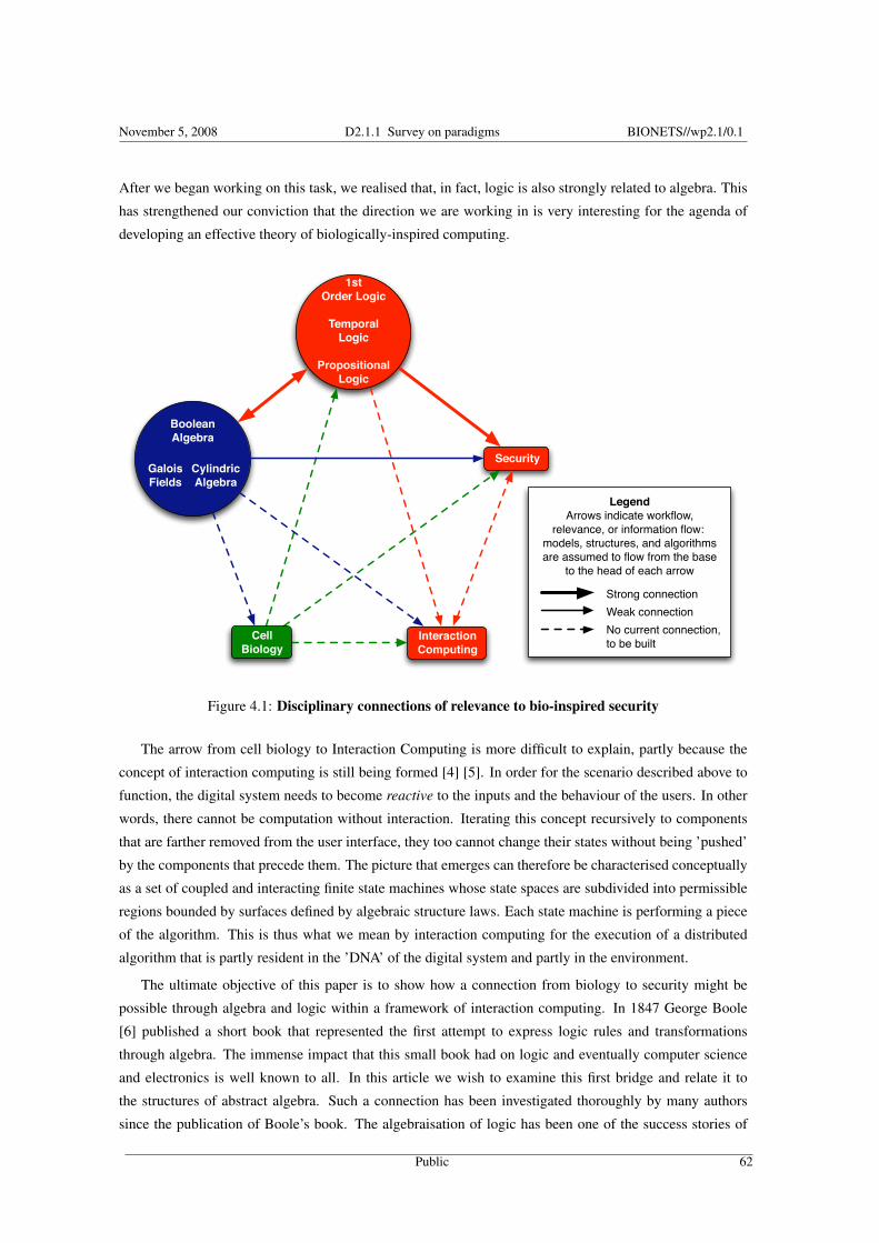
November 5, 2008 D2.1.1 Survey on paradigms BIONETS//wp2.1/0.1
After we began working on this task, we realised that, in fact, logic is also strongly related to algebra. This
has strengthened our conviction that the direction we are working in is very interesting for the agenda of
developing an effective theory of biologically-inspired computing.
Galois
Fields
Boolean
Algebra
Cylindric
Algebra
Temporal
Logic
Propositional
Logic
1st
Order Logic
Strong connection
No current connection,
to be built
Legend
Arrows indicate workflow,
relevance, or information flow:
models, structures, and algorithms
are assumed to flow from the base
to the head of each arrow
Security
Interaction
Computing
Cell
Biology
Weak connection
Figure 4.1: Disciplinary connections of relevance to bio-inspired security
The arrow from cell biology to Interaction Computing is more difficult to explain, partly because the
concept of interaction computing is still being formed [4] [5]. In order for the scenario described above to
function, the digital system needs to become reactive to the inputs and the behaviour of the users. In other
words, there cannot be computation without interaction. Iterating this concept recursively to components
that are farther removed from the user interface, they too cannot change their states without being ’pushed’
by the components that precede them. The picture that emerges can therefore be characterised conceptually
as a set of coupled and interacting finite state machines whose state spaces are subdivided into permissible
regions bounded by surfaces defined by algebraic structure laws. Each state machine is performing a piece
of the algorithm. This is thus what we mean by interaction computing for the execution of a distributed
algorithm that is partly resident in the ’DNA’ of the digital system and partly in the environment.
The ultimate objective of this paper is to show how a connection from biology to security might be
possible through algebra and logic within a framework of interaction computing. In 1847 George Boole
[6] published a short book that represented the first attempt to express logic rules and transformations
through algebra. The immense impact that this small book had on logic and eventually computer science
and electronics is well known to all. In this article we wish to examine this first bridge and relate it to
the structures of abstract algebra. Such a connection has been investigated thoroughly by many authors
since the publication of Boole’s book. The algebraisation of logic has been one of the success stories of
Public 62

November 5, 2008 D2.1.1 Survey on paradigms BIONETS//wp2.1/0.1
the 20th Century [7] [8] [9]. Therefore, we do not expect to say anything fundamentally new in this regard,
in this article. However, if we take the interface between algebra and logic to be the ’centre of gravity’
of this article, we are interested in shedding some light in two different directions. On the one hand, we
will review the mapping of propositional logic to Boolean algebra, briefly explain the algebraisation of
First-Order Logic, and finally show the link between First-Order and Temporal Logic, which is widely
used in the security domain to support applications that are able to describe, detect, and prevent specific
security features or breaches, respectively. On the other hand, we will review the fundamentals of abstract
algebra, touching on coding and Galois theory, in order to explore its connections to the interaction between
the DNA code and cell metabolism. In this manner we hope to begin charting a possible path from order
construction in biology to autonomic security algorithms and data structures that weaves its way through
algebra and logic.
4.2 Abstract Algebra
In this section we will present the very basics of abstract algebra, which is relevant to coding theory and
Galois theory. The objective is two-fold, i.e. to show how the structure of algebra resembles to some extent
the structure of logic, to be presented in the next chapter, and to provide a vocabulary and formalism that
will at a later date be applied to biology. In this short article we will not attempt to review and define an
isomorphic map between the parts of algebra and logic that are specifically relevant to biology and security,
mainly because this is still an open question. We will also not attempt to "solve" any cell biology problems.
The algebra discussed in this section is quite elementary because we think it is useful to have self-contained
discussion of the concepts alongside the review of logic and algebraic logic presented in Section 3 of this
article. Our purpose is to take the first tentative steps in the direction of an integrative formalism that we
hope will bear fruits over the life of the BIONETS project.
4.2.1 Starting Concepts
The language of abstract algebra is set theory. Since it is easy to read and understand for most people, it
is used here. Abstract algebra deals with the operations between the elements of a set, with the mappings
between different sets, and with mappings defined from a set to itself. Different kinds of operations and
mappings give rise to different relationships between these constitutive parts of algebra, which is partly
responsible for associating a structure with algebra. The elements of a set can be anything at all, including
other sets. They can be integers, polynomials, functions, ’variables’, and so forth. What Boole realised is
that they could also be the constitutive elements of logic, which provides one of the fundamental motivations
for the line of investigation pursued in this article. Finally, we are making an explicit assignment of some
yet unspecified elements of the cell as elements of a set. The temptation is to treat the cell itself as a set.
Although this is not necessarily wrong, we are starting with much simpler sets such as, for example, treating
the four bases of the DNA as the elements of a set that we can call the alphabet of DNA. Another example
could be the 20 amino-acids from which all proteins are built.
Algebra has successfully identified and formalised the fact that certain sets, although apparently differ-
ent on the surface, exhibit identical behaviour in how their elements relate to or combine with each other.
This motivates the definition of abstract ’objects’ that model the structure and/or behaviour of sets that
Public 63

November 5, 2008 D2.1.1 Survey on paradigms BIONETS//wp2.1/0.1
recur again and again in countless applications. We will now define these basic building blocks, relying
almost exclusively on examples from various sets of numbers (the integers Z, the real numbers R, etc) and
of polynomials. The following statements can be found in any algebra book, but we are borrowing freely
mainly from [10] [11] [12].
A binary relation is a statement which, for any two elements of a set, is either true or false for that pair.
Another way to put it is that a binary relation R on a set A is a subset of the Cartesian product A×A. For
example, if A = 1,2,3, then the relation ’less than’ on A is the set (1,2),(1,3),(2,3).
Let R be a binary relation on A. An equivalence relation is a binary relation that satisfies these three
conditions:
• (Reflexive) (a,a) ∈ R,∀a ∈ A
• (Symmetric) If (a,b) ∈ R, then (b,a) ∈ R
• (Transitive) If (a,b) ∈ R and (b,c) ∈ R, then (a,c) ∈ R
The equivalence class of the element a ∈ A is the set
b ∈ A : (a,b) ∈ R
In the example above, the relation ’less than’ fails all three properties, so it is not an equivalence relation.
An important fact that is not necessarily obvious is that the set of equivalence classes of a relation R on a
set A is a partition of A. In other words, the equivalence classes do not intersect and, together, they cover
all of A.
4.2.2 Groups, Rings and Fields
Before we can move forward we need to define three of the abstract objects, or types of set, that were
indicated above: groups, rings and fields.
A group is a set G of elements with a binary operation between them such that:
• (G0- Closure) ∀ g, h ∈ G, gh ∈ G
• (G1- Associative) g (h k) = (gh) k, ∀ (g, h, k) ∈ G
• (G2- Identity) ∃ e ∈ G : g e = eg = g, ∀g ∈ G
• (G3- Inverse) ∀ g ∈ G, ∃ h ∈ G : gh = hg = e
• (G4- Commutative) gh = hg, ∀(g, h) ∈ G
The last condition is satisfied only by so-called abelian or commutative groups.
A ring R is a set with two operations, that are usually called ’addition’ and ’multiplication’, such that:
• (A0- Closure) ∀ a, b ∈ R, a+b ∈ R
• (A1- Associative) a+(b+ c) = (a+b)+ c, ∀ (a, b, c) ∈ R
Public 64

November 5, 2008 D2.1.1 Survey on paradigms BIONETS//wp2.1/0.1
Operations+ ·
0 0 0 00 1 1 01 0 1 01 1 0 1
Table 4.1: Truth table for the Z2 field
• (A2- Zero) ∃ 0 ∈ R : a+0 = 0+a = a, ∀a ∈ R
• (A3- Inverse) ∀ a ∈ R, ∃ b ∈ R : a+b = b+a = 0
• (A4- Commutative) a+b = b+a, ∀(a, b) ∈ R
• (M0- Closure) ∀ a, b ∈ R, ab ∈ R
• (M1- Associative) a(bc) = (ab)c, ∀ (a, b, c) ∈ R
• (D- Distributive) (a+b)c = ac+bc, c(a+b) = ca+ cb∀ (a, b, c) ∈ R
Rings can have additional structure if they satisfy one or more of these additional axioms:
• (M2- Identity) ∃ 1 ∈ R(1 6= 0) : a1 = 1a = a, ∀a ∈ R
• (M3- Inverse) ∀ a ∈ R(a 6= 0), ∃ b ∈ R : ab = ba = 1
• (M4- Commutative) ab = ba, ∀(a, b) ∈ R
A ring that satisfies M2 is called a ring with identity. If it satisfies M2 and M3 it is called a divisionring. A ring that satisfies the first 8 axioms plus M4 is a commutative ring. A ring that satisfies all the
axioms, i.e. a commutative division ring with identity, is a field. Subrings and subfields are subsets of rings
or fields that are themselves rings or fields.
In preparation for the next section on logic, it is interesting to represent the field 0,1 using the lan-
guage of truth tables, as shown in Table 4.1.
4.2.3 Cosets and Homomorphisms
Now we are going to start building up some more complicated concepts using the basics defined so far. It
is probably fair to say that the previous section is an essential reference that we can go back to when the
derivations below get confusing, whereas Section 2.1 will be used right away.
The presentation of this material is necessarily abstract and a little dry. We will try to compensate for
this by spending extra effort in explaining the concepts thoroughly, whenever possible, since most of the
concepts are extremely interesting. Given also their great depth, however, in most cases we will not be
able to do justice to the beauty and broad relevance of the theory. We will use numbers and polynomials as
motivating examples, keeping an eye out for connections with logic, which is presented in the next chapter,
and with biology, which is presented in the last chapter.
Public 65
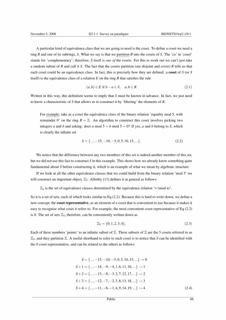
November 5, 2008 D2.1.1 Survey on paradigms BIONETS//wp2.1/0.1
A particular kind of equivalence class that we are going to need is the coset. To define a coset we need a
ring R and one of its subrings, S. What we say is that we partition R into the cosets of S. The ’co’ in ’coset’
stands for ’complementary’; therefore, S itself is one of the cosets. For this to work out we can’t just take
a random subset of R and call it S. The fact that the cosets partition (are disjoint and cover) R tells us that
each coset could be an equivalence class. In fact, this is precisely how they are defined: a coset of S (or S
itself) is the equivalence class of a relation E on the ring R that satisfies the rule
(a,b) ∈ E if b−a ∈ S, a,b ∈ R (2.1)
Written in this way, this definition seems to imply that S must be known in advance. In fact, we just need
to know a characteristic of S that allows us to construct it by ’filtering’ the elements of R.
For example, take as a coset the equivalence class of the binary relation ’equality mod 5, with
remainder 0’ on the ring R = Z. An algorithm to construct this coset involves picking two
integers a and b and asking: does a mod 5 = b mod 5 = 0? If yes, a and b belong to S, which
is clearly the infinite set
S = ...,−15,−10,−5,0,5,10,15, .... (2.2)
We notice that the difference between any two members of this set is indeed another member of this set,
but we did not use this fact to construct S in this example. This shows how we already know something quite
fundamental about S before constructing it, which is an example of what we mean by algebraic structure.
If we look at all the other equivalence classes that we could build from the binary relation ’mod 5’ we
will construct an important object, Z5. Allenby [11] defines it in general as follows:
Zn is the set of equivalence classes determined by the equivalence relation ’= (mod n)’.
So it is a set of sets, each of which looks similar to Eq (2.2). Because this is hard to write down, we define a
new concept, the coset representative, as an element of a coset that is convenient to use because it makes it
easy to recognise what coset it refers to. For example, the most convenient coset representative of Eq (2.2)
is 0. The set of sets Z5, therefore, can be conveniently written down as
Z5 = 0,1,2,3,4, (2.3)
Each of these numbers ’points’ to an infinite subset of Z. These subsets of Z are the 5 cosets referred to as
Z5, and they partition Z. A useful shorthand to refer to each coset is to notice that S can be identified with
the 0 coset representative, and can be related to the others as follows:
S = ...,−15,−10,−5,0,5,10,15, ...→ 0
S +1 = ...,−14,−9,−4,1,6,11,16, ...→ 1
S +2 = ...,−13,−8,−3,2,7,12,17, ...→ 2
S +3 = ...,−12,−7,−2,3,8,13,18, ...→ 3
S +4 = ...,−11,−6,−1,4,9,14,19, ...→ 4 (2.4)
Public 66
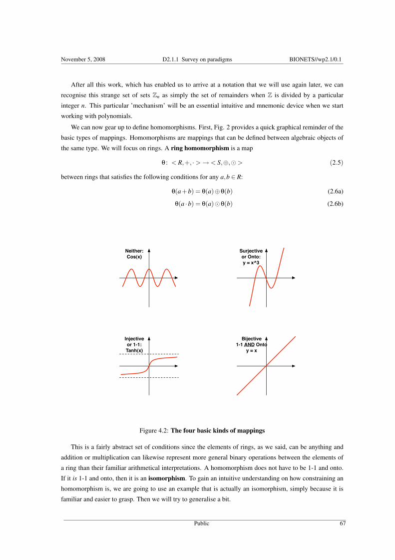
November 5, 2008 D2.1.1 Survey on paradigms BIONETS//wp2.1/0.1
After all this work, which has enabled us to arrive at a notation that we will use again later, we can
recognise this strange set of sets Zn as simply the set of remainders when Z is divided by a particular
integer n. This particular ’mechanism’ will be an essential intuitive and mnemonic device when we start
working with polynomials.
We can now gear up to define homomorphisms. First, Fig. 2 provides a quick graphical reminder of the
basic types of mappings. Homomorphisms are mappings that can be defined between algebraic objects of
the same type. We will focus on rings. A ring homomorphism is a map
θ : < R,+, ·>→ < S,⊕,¯> (2.5)
between rings that satisfies the following conditions for any a,b ∈ R:
θ(a+b) = θ(a)⊕θ(b) (2.6a)
θ(a ·b) = θ(a)¯θ(b) (2.6b)
Injective
or 1-1:
Tanh(x)
Surjective
or Onto:
y = x^3
Bijective
1-1 AND Onto
y = x
Neither:
Cos(x)
Figure 4.2: The four basic kinds of mappings
This is a fairly abstract set of conditions since the elements of rings, as we said, can be anything and
addition or multiplication can likewise represent more general binary operations between the elements of
a ring than their familiar arithmetical interpretations. A homomorphism does not have to be 1-1 and onto.
If it is 1-1 and onto, then it is an isomorphism. To gain an intuitive understanding on how constraining an
homomorphism is, we are going to use an example that is actually an isomorphism, simply because it is
familiar and easier to grasp. Then we will try to generalise a bit.
Public 67
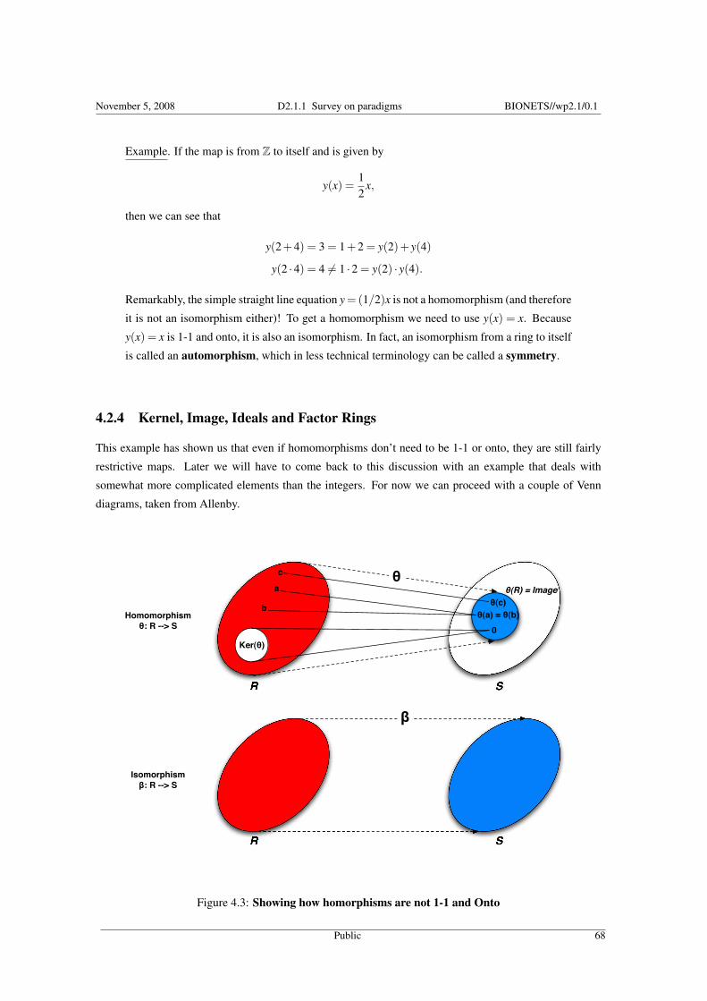
November 5, 2008 D2.1.1 Survey on paradigms BIONETS//wp2.1/0.1
Example. If the map is from Z to itself and is given by
y(x) =12
x,
then we can see that
y(2+4) = 3 = 1+2 = y(2)+ y(4)
y(2 ·4) = 4 6= 1 ·2 = y(2) · y(4).
Remarkably, the simple straight line equation y = (1/2)x is not a homomorphism (and therefore
it is not an isomorphism either)! To get a homomorphism we need to use y(x) = x. Because
y(x) = x is 1-1 and onto, it is also an isomorphism. In fact, an isomorphism from a ring to itself
is called an automorphism, which in less technical terminology can be called a symmetry.
4.2.4 Kernel, Image, Ideals and Factor Rings
This example has shown us that even if homomorphisms don’t need to be 1-1 or onto, they are still fairly
restrictive maps. Later we will have to come back to this discussion with an example that deals with
somewhat more complicated elements than the integers. For now we can proceed with a couple of Venn
diagrams, taken from Allenby.
Isomorphism
β: R --> S
R S
R S
θ(R) = Image
0
θ(a) = θ(b)Homomorphism
θ: R --> S
a
b
c
Ker(θ)
θ(c)
θ
β
Figure 4.3: Showing how homorphisms are not 1-1 and Onto
Public 68

November 5, 2008 D2.1.1 Survey on paradigms BIONETS//wp2.1/0.1
Figure 3 shows two new objects, the kernel and the image of a homomorphism. The kernel of a ring
homomorphism θ : R→ S is a subring of R defined by
Ker(θ) = k ∈ R : θ(k) = 0. (2.7)
The image is a subring of S defined by
Im(θ) = s ∈ S : s = θ(r) for some r ∈ R. (2.8)
There is a generalisation of the kernel that we are going to need. An ideal of a ring R is a subring S of R
such that, for any s ∈ S and r ∈ R, rs,sr ∈ S. To decide whether a subring is an ideal we should test this
condition plus all the ring axioms. However, there is an equivalent and shorter ’ideal test’. A non-empty
subset S of a ring R is an ideal of R iff
(a) ∀ s1,s2 ∈ S, s1− s2 ∈ S (2.9a)
(b) ∀ s ∈ S and r ∈ R, rs,sr ∈ S. (2.9b)
On the basis of this we can say that the kernel of a homomorphism θ : R→ S is an ideal of R. For example,
all the subrings of Z of the form nZ are ideals. We can now see how the first of the sets in Eq. (2.4) is
actually an ideal, which means that we can refer to the various cosets as I, I +1, I +2, etc. The ’set of sets’
that we keep referring to is so important that it is given a special name, the factor ring. Additionally, its
definition is made quite general, as follows.
Let I be an ideal of the ring R. The factor ring R/I is the set of cosets of I in R, with operations of
addition and multiplication defined as
(I + x)+(I + y) = I +(x+ y) (2.10a)
(I + x)(I + y) = I + xy (2.10b)
4.2.5 Fields
The research discussed in this article is not in mathematics, but in the application of algebra to logic, biology,
and new forms and models of computing. Therefore, practically no proofs are given and a lot is taken for
granted. We are just covering the smallest possible number of essential concepts in order to provide a basis
for coding theory and Galois theory that can expose the underlying algebraic machinery. We are assuming
that this algebraic machinery will then be relevant to biology, logic, and security. Furthermore, we hope
that it will help us develop a model for interactive computing that should enable the replication of biological
behaviour in software and in security applications in particular. Fields are the next algebraic structure that
will help us in this endeavour.
Whereas the ’ring archetype’ is the set of integers Z, the ’field archetype’ is the set of rational numbers,
Q. We saw in Section 2.2 that fields are more constrained than rings. In fact they are so constrained that
there are only two methods to construct a field. The first method essentially replicates the construction of
Q from Z. We proceed with a few definitions taken from [10].
A zero divisor in a ring R is a non-zero element a ∈ R : ∃(b 6= 0) ∈ R with ab = 0. An integral domainis a commutative ring with identity that has no zero-divisors (e.g. Z). Let R be an integral domain. A field
Public 69
November 5, 2008 D2.1.1 Survey on paradigms BIONETS//wp2.1/0.1
F is a ’field of fractions’ of R if
(a) R is a subring of F
(b) Any element of F can be written in the form ab−1 for some a,b ∈ R
The result of this kind of construction is an infinite field.
The second method generalises the construction of the integers modulo n from the integers, that is, the
field is a factor ring R/I. Some conditions need to be satisfied for this to be true, but in the examples we
will discuss it will be true, so we skip the finer points here. The result of this kind of construction is a finite
field.
Something we have not yet stated is that, for factor rings generated as a set of integers modulo n, n must
be a prime number. More generally, Galois proved that any and all finite fields have order a prime power.
This means that the number of elements of a finite field can only be either a prime (exponent = 1) or a
prime raised to a positive integer power. For example, finite fields of size 5, or 25, or 256 exist, whereas no
finite fields of size 18, or 30, or 100 exist. It is important to realise that, if the field is a prime power where
the power is greater than 1, then such a field cannot be composed by integers as its elements. As we will
soon see, in such cases its elements are more complex and can be represented as vectors, or as polynomials.
Finite fields are often called Galois fields in honour of their discoverer. Thus, Z5 can also be called GF(5)
and Z2 is interchangeable with GF(2). To denote a finite field whose size is a prime power, say m, we say
GF(2m). Such fields, where m > 1, are called field extensions.
4.2.6 Field Extensions
We have now reached the central topic of interest in this chapter, field extensions. Field extensions are
useful to give us a way to find the roots of polynomials. The kinds of problems we are interested in deal
with finite fields and with polynomials defined over finite fields, although the theory can handle any kind
of field. This means, for example, that if the finite field in question is F = 0,1,2,3,4, the polynomials
we can build have coefficients that can be taken only from this set of integers. Such polynomials are not
constrained in their degree, they can be of arbitrarily high degree. The (infinite) set of all such polynomials
is not a field, it is a ring with identity, denoted by F [x]. Since a ring needs to satisfy the closure condition
under addition and multiplication, when any two polynomials are added or multiplied together the arithmetic
operations on their coefficients are performed modulo (in this case) 5. This ensures closure with respect
to F . If a polynomial defined in this way has no roots in the field over which it is defined, it is called
irreducible. Polynomials whose leading coefficient (coefficient of the highest power of x) is 1 are called
monic polynomials.
We finally come to the main theorem of interest, due to Kronecker. Let F be any field and let f (x) =
a0 +a1x+a2x2 + ...+amxm ∈ F [x] be an irreducible polynomial over F. Then ∃ a field S containing F as a
subfield such that f (x) has a root in S. S is the extension field, F is the base field.
Surprising as it may seem, finding such a root is not our main goal! We will show why the above
theorem is true by relying on most of the concepts discussed so far, which is in itself quite interesting.
However, in the process we will discover that the roots of f (x) in the extension field have a very unexpected
representation, which makes them look rather useless. Our state of confusion will be rescued by a method
Public 70
November 5, 2008 D2.1.1 Survey on paradigms BIONETS//wp2.1/0.1
that shows how the algegraic structures in the extension field (the roots) are related to the algebraic structures
in the polynomial ring from which f (x) is taken through an elaborate mechanism [13]. This ’mechanism’
sheds light on network coding techniques, highlighting how they too do not need to find any roots explicitly.
In future work we will explore Gordon’s technique as it makes it relatively easy to verify the abstract theory
presented here with simple numerical examples. We will not have time or space in this article to delve into
Galois theory, which requires another level of abstraction and a firm grasp of groups, in addition to rings
and fields. The results we will discuss, however, should already provide a sufficiently rich context to begin
thinking about how to map them to security through logic, and to interaction computing through biology.
Our first step is to note that we can define an infinite number of ideals as subrings of F [x]. Each ideal
is generated by any one of the polynomials in the ring. For simplicity let’s assume that we are dealing
only with irreducible polynomials over F . We could take F to be the field GF(2) = 0,1 without loss of
generality. In other words, to prepare ourselves for the network coding examples (to be discussed in future
work) and the application to information systems in general we can use the binary ’alphabet’ as our base
field.
Kronecker’s theorem is proven by first establishing the following. Given a ring R and an ideal I of R,
∃ a ring S and a surjective map θ : R→ S such that Ker(θ) = I. This means that the polynomial of interest
(and all its possible multiples taken from F [x]) is mapped to 0 in S.
The ideal generated by a polynomial f (x) is the set of the possible products of all the elements of F [x]
with f (x), and is denoted by [ f (x)]. The ring S is nothing more than the factor ring
S =RI
=F [x][ f (x)]
, (2.11)
which is (conceptually) built by dividing all the polynomials in F [x] by the polynomial f (x) and retaining
only the remainders. Each different remainder represents a different coset representative for a different
coset of R. How many representatives are there? How big is S? It turns out it’s not that big.
For example, if the irreducible polynomial in question is of degree 6, the remainders can, by
definition, be of degree 5 at most:
a0 +a1x+a2x2 +a3x3 +a4x4 +a5x5. (2.12)
Because the coefficients are taken from Z2 = GF(2) this is equivalent to a binary string of 6
bits. Thus, there is a total of 26 = 64 elements in S for this example.
In other words, the required map is division of F [x] by f (x), modulo f (x). Because this maps F [x] to
the ring of remainders obtained by dividing by f (x), any multiple of f (x) will give 0 remainder. But any
multiple of f (x) is the ideal I = [ f (x)] generated by f (x). Therefore, I is mapped to the 0 element of S.
Therefore, Ker(θ) = I as required.
We can now prove Kronecker’s theorem. This is done in two steps: (1) we need to show that S = R/I
is a field; (2) we need to show that S contains a root of f (x). To prove the first part we first note that each
element of S is usually written as
I + r(x), (2.13)
Public 71
November 5, 2008 D2.1.1 Survey on paradigms BIONETS//wp2.1/0.1
where r(x) is the remainder we have been talking about. Now suppose that
f (x) = b0 +b1x+b2x2 + ...+bmxm (2.14)
and that r(x)+ I is a non-zero element of S. Because r(x) is a remainder upon division by f (x), necessarily
the Greatest Common Divisor in F [x] GCD(r(x), f (x)) = 1. One of the algebra basics we glossed over is
the result that, in F [x], ∃ s(x), t(x) :
s(x)r(x)+ t(x) f (x) = GCD
s(x)r(x)+ t(x) f (x) = 1 in F [x] (2.15)
Now the element 1 of R is mapped to the element 1 + I of S because clearly the number 1 can only be a
remainder in a division by f (x). Therefore, Eq. (2.15) in S becomes
s(x)r(x)+ t(x) f (x)+ I = 1+ I in S
By the rules by which ideals are added and multiplied (Eq. (2.10)),
[s(x)r(x)+ I]⊕ [t(x) f (x)+ I] = 1+ I in S,
[s(x)+ I]¯ [r(x)+ I]⊕ [t(x)+ I]¯ [ f (x)+ I] = 1+ I in S.
But, by the definition of ideal,
f (x)+ I = I = 0 in S!
As a consequence,
[s(x)+ I]¯ [r(x)+ I] = 1+ I in S, (2.16)
which means that the element [r(x)+ I] has an inverse in S:
[r(x)+ I]−1 = [s(x)+ I] in S. (2.17)
Hence, S is a field.
Now we need to show that S contains a root of f (x). To do this it is helpful to refer to Fig. 4, which is
also taken from Allenby. In the figure we can see how the original field F is a subset of F [x] since b0 in Eq
(2.14) spans over (can take on the value of) every element of F ; of course this refers to those polynomials
for which b1 and all the higher coefficients are 0, i.e. to constant polynomials. The map θ then involves
dividing all the polynomials in F [x] by a particular polynomial f (x), keeping only the remainders. Clearly,
all the constant polynomials can only be remainders. Therefore, the field F is identically reconstructed in
the factor ring S (which we have now established is a field). This is shown as θ(F) = F in the figure.
The final step in the proof is almost unremarkable and one struggles to see its significance at first. We
notice that we have constructed the field S in such a way as to make f (x) and its ideal map to 0. Then,
necessarily, the variable x must map to the root of f (x), which we will call α. How can we be sure? We
know that x is of degree smaller than f (x) because, if f (x) were a first-order polynomial then its root would
lie in F and we would have no need for all this work. So f (x) is of degree 2 or higher (and it is irreducible
Public 72
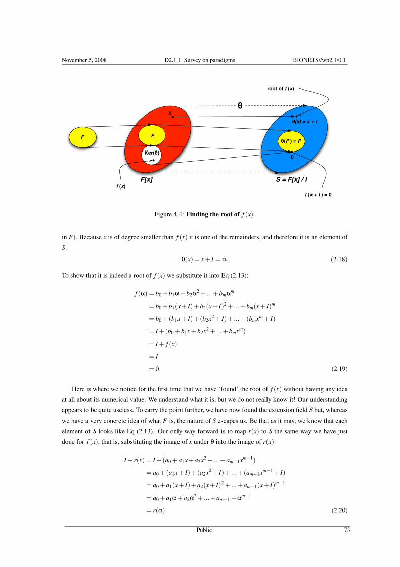
November 5, 2008 D2.1.1 Survey on paradigms BIONETS//wp2.1/0.1
F[x] S = F[x] / I
0
x
Ker(θ)
θ(x) = x + I
θ
Fθ(F ) = F
F
f (x)
f (x + I ) = 0
root of f (x)
Figure 4.4: Finding the root of f (x)
in F). Because x is of degree smaller than f (x) it is one of the remainders, and therefore it is an element of
S:
θ(x) = x+ I = α. (2.18)
To show that it is indeed a root of f (x) we substitute it into Eq (2.13):
f (α) = b0 +b1α+b2α2 + ...+bmαm
= b0 +b1(x+ I)+b2(x+ I)2 + ...+bm(x+ I)m
= b0 +(b1x+ I)+(b2x2 + I)+ ...+(bmxm + I)
= I +(b0 +b1x+b2x2 + ...+bmxm)
= I + f (x)
= I
= 0 (2.19)
Here is where we notice for the first time that we have ’found’ the root of f (x) without having any idea
at all about its numerical value. We understand what it is, but we do not really know it! Our understanding
appears to be quite useless. To carry the point further, we have now found the extension field S but, whereas
we have a very concrete idea of what F is, the nature of S escapes us. Be that as it may, we know that each
element of S looks like Eq (2.13). Our only way forward is to map r(x) to S the same way we have just
done for f (x), that is, substituting the image of x under θ into the image of r(x):
I + r(x) = I +(a0 +a1x+a2x2 + ...+am−1xm−1)
= a0 +(a1x+ I)+(a2x2 + I)+ ...+(am−1xm−1 + I)
= a0 +a1(x+ I)+a2(x+ I)2 + ...+am−1(x+ I)m−1
= a0 +a1α+a2α2 + ...+am−1−αm−1
= r(α) (2.20)
Public 73

November 5, 2008 D2.1.1 Survey on paradigms BIONETS//wp2.1/0.1
The result tells us that each element of S is isomorphic to the remainders of F [x]/[ f (x)], but expressed in
terms of the root we have ’found’. Interestingly, we have discovered quite a bit about the extension field
of F without calculating any ’numbers’. The nature of the extension field S is in fact to be isomorphic to a
vector space of dimension 2m over the field F . In other words, since F = GF(2), S = GF(2m). The different
powers of the root α play the role of basis vectors. We recognise in this the same structure of the complex
field C, each of whose elements is of the form a+ ib, where i is the root of the polynomial x2 +1, which is
irreducible over the real field R.
4.3 Logic, Algebra, and Security
Having presented a general overview of abstract algebra and its very basic concepts, this section is going to
establish a link between the disciplines of logic, algebra, and security.
For this purpose we start by defining propositional and first-order logic. Section 2 should help see the
strong similarities between logic and algebra, especially when comparing Galois fields and propositional
logic. We will attempt to show how the different logics find their counterparts in the realm of abstract
algebra. With the informal extension of the basic concepts of logic and algebra to temporal logic and
quantifier algebras, respectively, we will bridge from algebra to security. This not entirely obvious bridge is
emphasized in the final sub-section, where we show that the intentional application of temporal logic and its
wide use in the realm of computer science is process and program analysis and is therefore directly linked
to security.
4.3.1 Propositional and First-Order Logic
In this section we want to give a short introduction to propositional and predicate logic, two important fields
of the research area of symbolic logic. Of course, this introduction cannot be exhaustive and we will refer
the reader to appropriate literature.
The following sub-section will be the basis for sub-sections 4.3.2 and 4.3.3. However, for the experi-
enced reader who is familiar with the basic concepts of these logics we recommend to proceed directly to
sub-section 4.3.2.
Propositional Logic
Propositional logic is often called sentential logic. Both names account for the nature of this logic since it
uses sentences, thus sentential, which can be thought of as propositions. The classical propositional logic
studies the effects of propositional connectives, such as and and or, which can be used to form new sentences
out of atomic sentences. To formalise this quantitative description we define the syntax of propositional
logic before defining its semantics.
For the following definitions we assume that P is an infinite (countable) alphabet of propositional letters.
Additionally we denote > and ⊥ for the values true and false as it is usually done in classical two-valued
logic. Based on these assumptions we define propositional atomic formulas and propositional formulas.
Definition 4.3.1 An atomic formula is a propositional letter, > or ⊥.
Public 74

November 5, 2008 D2.1.1 Survey on paradigms BIONETS//wp2.1/0.1
Connectives⊥ ∧ ⊇ L ⊆ R 6≡ ∨ ↓ ≡ ¬ R ⊂ ¬ L ⊃ ↑ >
0 0 0 0 0 0 0 0 0 0 1 1 1 1 1 1 1 10 1 0 0 0 0 1 1 1 1 0 0 0 0 1 1 1 11 0 0 0 1 1 0 0 1 1 0 0 1 1 0 0 1 11 1 0 1 0 1 0 1 0 1 0 1 0 1 0 1 0 1
Table 4.2: Definition of propositional logic connectives
Please note that > and ⊥ are currently only symbols without any interpretation.
Definition 4.3.2 The set of propositional formulas is the smallest set P such that
1. If A is an atomic formula, A ∈ P
2. X ∈ P ⇒¬X ∈ P
3. If is a binary symbol, then X ,Y ∈ P ⇒ (X Y ) ∈ P
These definitions are sufficient to define the syntax of propositional logic. Due to space constraints, we
skip numerous theorems and other definitions that facilitate the handling of propositional logic. Instead, we
now define its semantics. To do so we first have to define so-called truth values, which can be mapped to
our previously defined truth symbols. For this purpose we define the set T = 0,1. Looking at definition
4.3.2 we additionally have to define the operation on set T represented by the operation symbols ¬ and .
There are some similarities and differences between these definitions and the starting point of abstract
algebra. P is analogous to an infinite set of variables whose values are taken from the field Z2 = T . In
abstract algebra we define more complicated ’objects’ over a particular field. These objects are called
polynomials. So we can have polynomials over Z2 or over Z,N,Q,R,C. In propositional logic we do not
actually have objects as complicated as polynomials, we have sets of propositions that are connected by
various binary or unary operators, forming the ’sentences’ mentioned above.
For the operational symbol ¬ we define the mapping ¬ : T → T by ¬(t) = f and ¬( f ) = t. Defining
the binary connectives is more complicated as there are 16 possible mappings. We can enumerate the
definitions of all connectives in Table 4.2.
After defining the basic operations of propositional logic we can now define the so-called Boolean
valuation, which is an appropriate mapping for propositional formulas.
Definition 4.3.3 A Boolean valuation is a mapping v from the set of propositional formulas to the set Tmeeting the conditions
1. v(>) = 1;v(⊥) = 0
2. v(¬X) = ¬v(X)
3. v(X Y ) = v(X) v(Y ), for any binary operations
Public 75
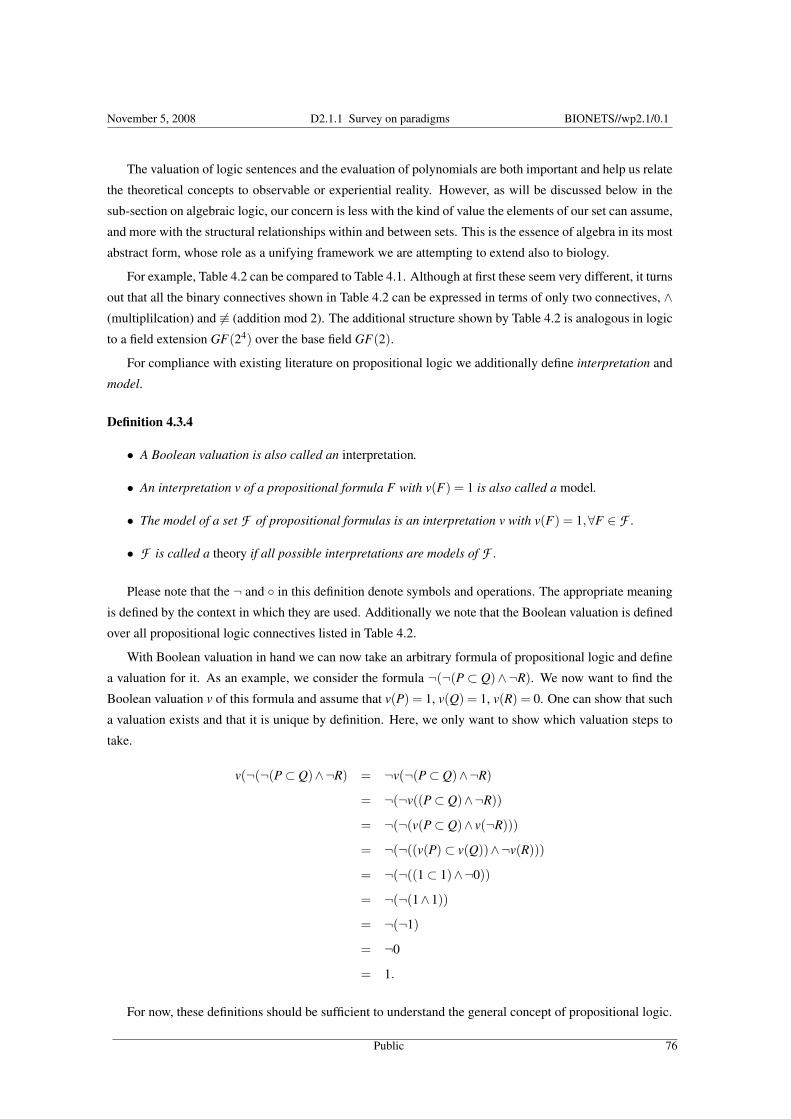
November 5, 2008 D2.1.1 Survey on paradigms BIONETS//wp2.1/0.1
The valuation of logic sentences and the evaluation of polynomials are both important and help us relate
the theoretical concepts to observable or experiential reality. However, as will be discussed below in the
sub-section on algebraic logic, our concern is less with the kind of value the elements of our set can assume,
and more with the structural relationships within and between sets. This is the essence of algebra in its most
abstract form, whose role as a unifying framework we are attempting to extend also to biology.
For example, Table 4.2 can be compared to Table 4.1. Although at first these seem very different, it turns
out that all the binary connectives shown in Table 4.2 can be expressed in terms of only two connectives, ∧(multiplilcation) and 6≡ (addition mod 2). The additional structure shown by Table 4.2 is analogous in logic
to a field extension GF(24) over the base field GF(2).
For compliance with existing literature on propositional logic we additionally define interpretation and
model.
Definition 4.3.4
• A Boolean valuation is also called an interpretation.
• An interpretation v of a propositional formula F with v(F) = 1 is also called a model.
• The model of a set F of propositional formulas is an interpretation v with v(F) = 1,∀F ∈ F .
• F is called a theory if all possible interpretations are models of F .
Please note that the ¬ and in this definition denote symbols and operations. The appropriate meaning
is defined by the context in which they are used. Additionally we note that the Boolean valuation is defined
over all propositional logic connectives listed in Table 4.2.
With Boolean valuation in hand we can now take an arbitrary formula of propositional logic and define
a valuation for it. As an example, we consider the formula ¬(¬(P ⊂ Q)∧¬R). We now want to find the
Boolean valuation v of this formula and assume that v(P) = 1, v(Q) = 1, v(R) = 0. One can show that such
a valuation exists and that it is unique by definition. Here, we only want to show which valuation steps to
take.
v(¬(¬(P⊂ Q)∧¬R) = ¬v(¬(P⊂ Q)∧¬R)
= ¬(¬v((P⊂ Q)∧¬R))
= ¬(¬(v(P⊂ Q)∧ v(¬R)))
= ¬(¬((v(P)⊂ v(Q))∧¬v(R)))
= ¬(¬((1⊂ 1)∧¬0))
= ¬(¬(1∧1))
= ¬(¬1)
= ¬0
= 1.
For now, these definitions should be sufficient to understand the general concept of propositional logic.
Public 76

November 5, 2008 D2.1.1 Survey on paradigms BIONETS//wp2.1/0.1
First-Order Logic
As we have seen above, propositional logic can be used to build formulas which represent propositions.
They can be evaluated using Boolean valuation. However, propositional logic is unable to derive valid
arguments which respect the internal structure of a proposition.
For this reason first-order logic (FOL) replaces the pure propositional letters by predicates which can
have arguments. Thus, first order logic is often called predicate logic. Due to the introduction of variables
FOL also supports quantifiers to bind variables.
As in the last subsection we will shortly introduce the syntax of first-order logic, also called first-order
language. After introducing the general concept of a model we define the semantics of FOL.
Definition 4.3.5 A first-order language L(R ,F ,C ) is determined by specifying
1. A finite or countable set R of relation symbols (predicate symbols) each of which has associated a
positive integer n with it. n indicates the arity1 of the predicate.
2. A finite or countable set F of function symbols each of which has associated a positive integer m with
it. m indicates the arity of the function.
3. A finite or countable set C of constant symbols.
Since we have finer granularity than in propositional logic, we have to define so-called terms before we
can take the next step and define first-order formulas, which are analogous to propositional logic formulas.
For this purpose we have to introduce variables. They represent elements of a set which we will later call
domain.
Definition 4.3.6 The family of terms of L(R ,F ,C ) is the smallest set meeting the following conditions:
1. Any variable is a term of L(R ,F ,C ).
2. Any c ∈ C is a term of L(R ,F ,C).
3. If f ∈F has arity n and t1, t2, ..., tn are terms of L(R ,F ,C ), then f (t1, t2, ..., tn) is a term of L(R ,F ,C).
4. We denote TL(R ,F ,C ) as the set of terms of L(R ,F ,C ).
Terms are closed if they contain no variables.
Based on the terms defined above we can now define formulas. You will recognise that the definition
is very similar to the definition of formulas in propositional logic. The main difference is the use of terms
instead of propositions and the introduction of the universal (∀) and existential (∃) quantifiers. We again
define atomic formulas first.
Definition 4.3.7 An atomic formula of L(R ,F ,C ) is any string of the form R(t1, t2, ..., tn) with R ∈ R and
t1, t2, ..., tn ∈ TL(R ,F ,C )
1In logic, mathematics, and computer science, the arity of a function or operation is the number of arguments or operands that thefunction takes. The arity of a relation is the number of domains in the corresponding Cartesian product. In this research we focus onthe Cartesian product of a set with itself (A×A). For example, the arity of the addition operation is 2, which means that addition is abinary operation, or that it takes 2 arguments. (http://en.wikipedia.org/wiki/Arity)
Public 77
November 5, 2008 D2.1.1 Survey on paradigms BIONETS//wp2.1/0.1
Based on atomic formulas we define the family of formulas of L(R ,F ,C ).
Definition 4.3.8 The family of formulas of L(R ,F ,C ) is the smallest set meeting the following conditions
1. Any atomic formula of L(R ,F ,C ) is a formula of L(R ,F ,C )
2. If A is formula of L(R ,F ,C ) so is ¬A
3. For a binary connective , if A and B are formulas of L(R ,F ,C ) so is (AB).
4. If A is a formula of L(R ,F ,C ) and x is a variable, then (∀x)A and (∃x)A are formulas of L(R ,F ,C ).
By using the syntax defined above and defining R , F , and C appropriately we can specify the same
formulas that we find in popular theories such as set theory. Theories using this first-order language are also
called first-order theories.
But with the syntax alone, the language is rather useless as it has no meaning. Thus the next step is to
define a semantics. However, compared to propositional logic the definition of first-order logic semantics
is very complicated as we are facing variables, functions, relations, and quantifiers. To slightly simplify the
definition we will first introduce the concepts of models, which implicitly define domains and interpreta-
tions.
Definition 4.3.9 A model for the first-order language L(R ,F ,C ) is a pair M =< D,I > with
D is non-empty set, called a domain of M
I is a mapping, called an interpretation that associates
1. To every c ∈ C , some member cI ∈D
2. To every f ∈ F , some function f I : Dn →D
3. To every P ∈ R , some relation PI ⊆Dn
As we can see, models do not cover variables. But as terms in first-order language are based on variables
we also need to assign elements from a domain to terms in order to be able to associate a value with them.
Definition 4.3.10 Let M =< D,I > be a model for the language L(R ,F ,C ), and let A be an assignment
in M . To each t ∈ TL(R ,F ,C ) we associate a value tI ,A in D as follows:
1. For c ∈ C ,cI ,A ∈ cI
2. For a variable v,vI ,A = vA
3. For f ∈ F , [ f (t1, t2, ..., tn)]I ,A = f I (tI ,A1 , tI ,A
2 , ..., tI ,An )
By defining how each term is associated with a value we arrived at the point where it is possible to as-
sociate a truth value with each formula defined in L(R ,F ,C ). This can be done in analogy to propositional
logic. We are also going to use the same propositional constants > and ⊥ as well as the same connectives
(denoted as ) as in propositional logic.
Public 78
November 5, 2008 D2.1.1 Survey on paradigms BIONETS//wp2.1/0.1
Definition 4.3.11 Let M =< D,I > be a model for L(R ,F ,C ). Let A be an assignment in this model. To
each formula Φ of L(R ,F ,C ) we associate a value ΦI ,A ∈ T as follows:
1. For atomic cases
[P(t1, t2, ..., tn)]I ,A = t ⇔< tI ,A1 , tI ,A
2 , ..., tI ,An >∈ PI ,
>I ,A = t,
>I ,A = f .
2. [¬X ]I ,A = ¬[XI ,A ].
3. [X Y ]I ,A = XI ,A Y I ,A
4. [(∀x)Φ]I ,A = t ⇔ΦI ,B = t for every assignment B in M that is an x-variant of A .
5. [(∃x)Φ]I ,A = t ⇔ΦI ,B = t for some assignment B in M that is an x-variant of A .
Here the assignment B in the model M is an x-variant of the assignment A , if A and B only assign a
possibly different value to x.
We want to finish this sub-section by giving an example to illustrate the expressiveness of first-order
logic.
For this example we assume the language L(R,⊕, /0) with variables x and y. We choose M =<
N,I > as the model with I defined as follows:
1. ⊕I (a,b) = a+b, with a,b ∈ N, and
2. RI = (x,y) : x,y ∈ N,x > y
Now, consider the sentence (∀x)(∀y)(∃z)R(x⊕ y,z). It is easy to see that this sentence always evaluates
to truth value 1 in model M . Note that this valuation does not depend on the assignment as all variables in
this sentence are bound to a quantifier.
As for propositional logic we could now start to introduce proof procedures which would show the full
power of first-order logic. However, we skip these interesting details and refer the interested readers to [14].
4.3.2 Algebraic Logic
Algebraic Logic is the field of research which deals with studies of algebras that are relevant for logic. It
additionally investigates the methodology of solving problems in one of the two domains, algebra or logic,
and translating the solution back into its original domain.
This section is going to show how propositional logic as well as first order logic are connected to algebra.
Propositional Logic and Boolean Algebra
In sub-section 4.3.1 we introduced the basic syntax and semantic of propositional logic. We defined Boolean
evaluation and showed how a simple formula in propositional logic is valuated. If we want to generalize
the Boolean valuation for arbitrary formulas with n propositions we will have to investigate 2n different
interpretations.
Public 79
November 5, 2008 D2.1.1 Survey on paradigms BIONETS//wp2.1/0.1
This characteristic becomes a problem if we do not simply want to valuate propositional formulas but if
we want to draw logical consequences from them.
Definition 4.3.12 A propositional formula X is a logical (propositional) consequence of a set S of propo-
sitional formulas, provided that every model of S is also a model for X. We write S |=p X
In common language we could state that a logical consequence is a statement which follows from some
other statements. In mathematics, for example, the set of statements could be axioms.
So if we want to prove in propositional logic that a statement is a logical consequence of other propo-
sitional formulas one may use established proof procedures such as Hilbert systems or resolution. Logical
consequences can also be interpreted as a means to find propositional formulas which are equivalent, this
is, which have the same model. In the field of electronic circuits this is important as it allows to reduce cost
and to find formulas with the least number of connectives in it. This may be achieved by simply guessing
formulas and proving their logical equivalence by valuation.
In section 4.2 we discussed the basic concepts of abstract algebra. We learnt that the basic language of
abstract algebra is set theory and that algebra can be used to apply transformations to sets without destroying
the relations between the elements within the set (homomorphism, isomorphism, etc). With this motivation
we take a closer look at propositional logic.
Due to the definition of propositional logic any propositional formula has infinite equivalent formulas.
As an example consider the atomic formula which consists of the proposition P. This formula can easily
be extended with the propositional letter ⊥ to P∨⊥. Both formulas are equivalent as they have the same
model. If we now merge all propositional formulas that we can build from the propositions P and R and that
have the same model as P, we obtain a set that represents an equivalence class of propositional formulas
with model M. Obviously, we can group all propositional formulas based on the propositions in P = P,Rand obtain 16 equivalence classes. We call the set of these classes, set E .
Now, according to the notion of algebra, we look at the interrelation between these equivalence classes.
For this purpose we introduce a tautology and the concept of satisfiability.
Definition 4.3.13 A propositional formula X is a tautology if v(X) = 1 for every interpretation v.
Definition 4.3.14 A set S of propositional formulas is satisfiable if there is some interpretation v: v(s) =
1, ∀s ∈ S .
Thus, the propositional formula P∨¬P is a tautology. Consequently, we also find an equivalence class
that only contains tautologies. As v(>) = 1 for all interpretations v, we call this equivalence class [>]. Its
counterpart is the equivalence class which is not satisfiable. We denote this equivalence class with [⊥].
Intuitively, we now want to define a partial order on E . We define the order ≤ as follows:
X ≤ Y ⇔ v(P) = v(P∧R),∀P ∈ X and ∀R ∈ Y , with X ,Y ∈ E and f or all interpretations v.
Why is this an intuitive definition? Consider the valuation of formula P∧R with the interpretation v with
v(P) = > and v(R) = ⊥. This yields v(>∧⊥) = v(⊥) which also means that ⊥ ≤ > which would be an
intuitive definition of a relation on the set ⊥,>.
Public 80
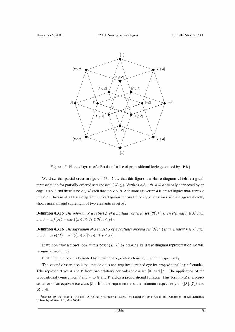
November 5, 2008 D2.1.1 Survey on paradigms BIONETS//wp2.1/0.1
u[⊥]
PPPPPPPPP³³³³³³³³³
BBBBBBBBB£
££££££££
u[P∧R]
³³³³³³³³³
£££££££££B
BBBBBBBB u
[P ↓ R]
PPPPPPPPP
BBBBBBBBB£
££££££££
u[P≡ R]
£££££££££B
BBBBBBBB
u[P 6⊃ R]
³³³³³³³³³PPPPPPPPP u[P 6⊂ R]
³³³³³³³³³PPPPPPPPP
u[P] ³³³³³³³³³
u[R] ³³³³³³³³³
u [¬R]
PPPPPPPPP u [¬P]
PPPPPPPPP
u[P⊂ R]
³³³³³³³³³
u[P⊃ R]
³³³³³³³³³PPPPPPPPP
u[P 6≡ R]
BBBBBBBBB£
££££££££
u[P∨R] PPPPPPPPP
BBBBBBBBB£
££££££££
u [P ↑ R]
³³³³³³³³³
£££££££££BB
BBBBBBB
u[>]
³³³³³³³³³PPPPPPPPP
£££££££££BB
BBBBBBB
Figure 4.5: Hasse diagram of a Boolean lattice of propositional logic generated by P,R
We draw this partial order in figure 4.52 . Note that this figure is a Hasse diagram which is a graph
representation for partially ordered sets (posets) (H ,≤). Vertices a,b ∈H ,a 6= b are only connected by an
edge if a≤ b and there is no c ∈H such that a≤ c≤ b. Additionally, vertex b is drawn higher than vertex a
if a≤ b. The use of a Hasse diagram is advantageous for our following discussions as the diagram directly
shows infimum and supremum of two elements in set H .
Definition 4.3.15 The infimum of a subset S of a partially ordered set (H ,≤) is an element h ∈ H such
that h = in f (H ) = max(x ∈H |∀y ∈H ,x≤ y).
Definition 4.3.16 The supremum of a subset S of a partially ordered set (H ,≤) is an element h ∈H such
that h = sup(H ) = min(x ∈H |∀y ∈H ,y≤ x).
If we now take a closer look at this poset (E ,≤) by drawing its Hasse diagram representation we will
recognize two things.
First of all the poset is bounded by a least and a greatest element, ⊥ and > respectively.
The second observation is not that obvious and requires a trained eye for propositional logic formulas.
Take representatives X and Y from two arbitrary equivalence classes [X ] and [Y ]. The application of the
propositional connectives ∨ and ∧ to X and Y yields a propositional formula. This formula Z is a repre-
sentative of an equivalence class [Z]. It is the supremum and the infimum respectively of [X ], [Y ] and
[Z] ∈ E .2Inspired by the slides of the talk “A Refined Geometry of Logic” by David Miller given at the Department of Mathematics,
University of Warwick, Nov 2005
Public 81
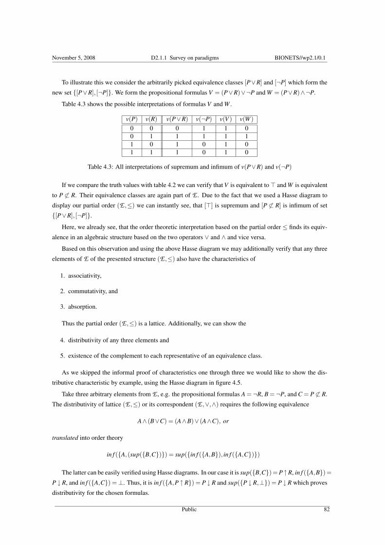
November 5, 2008 D2.1.1 Survey on paradigms BIONETS//wp2.1/0.1
To illustrate this we consider the arbitrarily picked equivalence classes [P∨R] and [¬P] which form the
new set [P∨R], [¬P]. We form the propositional formulas V = (P∨R)∨¬P and W = (P∨R)∧¬P.
Table 4.3 shows the possible interpretations of formulas V and W .
v(P) v(R) v(P∨R) v(¬P) v(V ) v(W )0 0 0 1 1 00 1 1 1 1 11 0 1 0 1 01 1 1 0 1 0
Table 4.3: All interpretations of supremum and infimum of v(P∨R) and v(¬P)
If we compare the truth values with table 4.2 we can verify that V is equivalent to> and W is equivalent
to P 6⊂ R. Their equivalence classes are again part of E . Due to the fact that we used a Hasse diagram to
display our partial order (E ,≤) we can instantly see, that [>] is supremum and [P 6⊂ R] is infimum of set
[P∨R], [¬P].
Here, we already see, that the order theoretic interpretation based on the partial order ≤ finds its equiv-
alence in an algebraic structure based on the two operators ∨ and ∧ and vice versa.
Based on this observation and using the above Hasse diagram we may additionally verify that any three
elements of E of the presented structure (E ,≤) also have the characteristics of
1. associativity,
2. commutativity, and
3. absorption.
Thus the partial order (E ,≤) is a lattice. Additionally, we can show the
4. distributivity of any three elements and
5. existence of the complement to each representative of an equivalence class.
As we skipped the informal proof of characteristics one through three we would like to show the dis-
tributive characteristic by example, using the Hasse diagram in figure 4.5.
Take three arbitrary elements from E , e.g. the propositional formulas A = ¬R, B = ¬P, and C = P 6⊂ R.
The distributivity of lattice (E ,≤) or its correspondent (E ,∨,∧) requires the following equivalence
A∧ (B∨C) = (A∧B)∨ (A∧C), or
translated into order theory
in f (A,(sup(B,C)) = sup(in f (A,B), in f (A,C))
The latter can be easily verified using Hasse diagrams. In our case it is sup(B,C)= P ↑R, in f (A,B)=
P ↓ R, and in f (A,C) =⊥. Thus, it is in f (A,P ↑ R) = P ↓ R and sup(P ↓ R,⊥) = P ↓ R which proves
distributivity for the chosen formulas.
Public 82

November 5, 2008 D2.1.1 Survey on paradigms BIONETS//wp2.1/0.1
The five characteristics listed above represent the axioms which have been set up by George Boole.
Therefore, this distributive complemented lattice is also called a Boolean algebra.
Tarski and Lindenbaum were the first to precisely discuss the set of propositional formulas as an algebra
with operators which were induced by the connectives of the propositional language. The structural analysis
we tried to sketch above by using intuition and geometrical representation in Hasse diagrams is discussed
in more detail in [8, 15].
We generalize this result and give the definition for a Boolean algebra.
Definition 4.3.17
A Boolean algebra is a structure B =< B,+, ·, ,0,1 > where the following system of equations is valid,
and where x,y,z ∈ B:
x+(y+ z) = (x+ y)+ z
x+ y = y+ x
x+(x · y) = x
x+(y · z) = (x+ y) · (x+ z)x+ x = 1
x · (y · z) = (x · y) · zx · y = y · x
x · (x+ y) = x
x · (y+ z) = (x · y)+(x · z)x · x = 0
(associativity)(commutativity)
(absorption)(distributivity)
(existence o f complement)
With this mathematical structure the Boolean algebra for propositional logic (PL) can be defined as the
Boolean algebra model BPL =< E ,∨,∧,¬, [⊥], [>] >.
You will realize that this algebra is only based on the operators ∨, ∧, and ¬. As we have shown the
equivalence with propositional logic is still valid. However, it becomes even more obvious if we reassure
the reader that every propositional formula can be rewritten into an equivalent propositional formula in
normal form which is only based on the connectives ∨ and ∧.
Summarizing the results of this section we can state that with Boolean algebra we possess a very power-
ful tool which can be used to transform arbitrary propositional formulas into other propositional and equiv-
alent formulas. These equivalence transformations have numerous areas of applications, such as integrated
circuit optimization or theorem proving to name just two possible domains.
However, of major importance for this contribution is the observation that there is a strong link between
propositional logic and algebra. We saw that the definition and structure of propositional logic directly
induces a Boolean algebra. Thus, we are now capable to choose a domain, propositional logic or Boolean
algebra, which offers the most suitable tools and the best knowledge to analyze a structure. Consequentially,
it would be good if the same correspondence between first-order logic and algebra held.
First-Order Logic and Quantifier Algebras
In this section we are going to show that first-order logic also possesses an algebraization. As we can use the
results from the last section we forego an intuitive interpretation and graphical explanation and use a more
mathematical approach. Nevertheless, this section is going to avoid complicated and highly mathematical
algebraizations of first order logic and follows the spirit of Charles C. Printer who followed “... the most
satisfactory way of introducing the [...] non-specialist to the ideas and methods of algebraic logic” [16].
Public 83

November 5, 2008 D2.1.1 Survey on paradigms BIONETS//wp2.1/0.1
From section 4.3.1 we already know that first-order logic is able to express formulas which are not
expressible in propositional logic. This is basically due to the fact that propositional logic has been extended
by quantifiers and that it supports n-ary relations as opposed to strict bi-nary relations. Now, one may
assume that we simply extend the Boolean algebra, the algebraization of propositional logic, and obtain a
first-order logic algebra. In the next couple of paragraphs this is exactly what we are going to do.
For this purpose we first introduce quantifier algebras for formulas. Their definition is very similar to
the construction of a Boolean algebra out of propositional logic. Thus, from the last section we simply
collect the elements which we need for a formal definition.
Let Γ be the first-order language L(R ,F ,C ) and let < vκ >κ<α a sequence of variables. Let Θ be a
theory of Γ. We define F Γ as the set of all formulas of Γ. We currently have to restrict our considerations
to the set of formulas which does not contain the formulas F ≡Θ G. Here relation ≡Θ denotes the equality
relation which can be deduced from Θ. This set is denoted by F Γ/≡Θ. We will account for this restriction
later in this section.
Based on L(R ,F Γ/ ≡Θ,C ) and the general Boolean algebra B =< B,+, ·, ,0,1 > we can define the
following Boolean operations:
(F/≡)+(G/≡) = F ∨G/≡(F/≡) · (G/≡) = F ∧G/≡
(F/≡) = ¬F/≡
1 denotes all formulas of theory Θ. For simplicity and consistency with previous sections we write>. 0, the
negations of all formulas in > is denoted by ⊥. We obtain the Boolean algebra < F Γ/≡Θ,+, ·, ,⊥,>>.
To define quantifier algebras we are only missing two more operations which find their analogy in the
quantifiers in first-order logic. For ∃we define the operation ∃κ with ∃κ(F/≡) denotes the equivalence class
of all formula (∃vκ)F . Quantifier ∀ can not be defined directly. Instead we define a substitution operation Sκλ.
Sκλ(F/≡) denotes the equivalence class of the formula which results from F by replacing each free occur-
rence of vκ by vλ. Here it becomes obvious why we needed an ordered sequence of variables. Extending the
Boolean algebra above we obtain the quantifier algebra of formulas: < F Γ/≡Θ,+, ·, ,⊥,>,Sκλ,∃κ >κ,λ<α
associated with Θ. We now formally define this algebra:
Definition 4.3.18 By a quantifier algebra of degree α (QAα) we mean a structure
U =< A,+, ·, ,0,1,Sκλ,∃κ >κ,λ<α where < A,+, ·, ,0,1 > is a Boolean Algebra with the unary opera-
tors Sκλ and ∃κ which have the following properties for all x,y ∈ A and κ,γ,λ < α,α≥ 2:
(q1) Sκλ(x) = Sκ
λ(x)(q2) Sκ
λ(x+ y) = Sκλ(x)+Sκ
λ(y)(q3) Sκ
κ(x) = x
(q4) SκλSγ
κ
(q5) ∃κ(x+ y) = ∃κx+∃κy
(q6) x≤ ∃κx
(q7) Sκλ∃κ = ∃κ
(q8) ∃κSκλ = Sκ
λ i f κ 6= λ(q9) Sκ
λ∃γ = ∃γSκλ i f γ 6= κ,λ
Public 84
November 5, 2008 D2.1.1 Survey on paradigms BIONETS//wp2.1/0.1
Due to the many indexes these equations may at first look difficult but if you have a closer look you
will realize that you can group (q1)− (q4) into simple substitution properties, (q5)− (q6) into quantifier
properties, and (q7)− (q9) into a group which relate substitutions to quantifiers. We assume here that the
interpretation of these equations is obvious.
If U is a quantifiere algebra as defined above we can define a so called dimension set of a fomula a ∈ A:
¦x = κ < α : ∀λ 6= κ, Sκλx 6= x
Quantitatively this is the set of all indexes κ of variables vκ which would change the valuation of formula
x if substituted with another variable vλ. We define U to be locally finite if ¦x is a finite set.
It can be shown that every quantifier algebra of formulas is a locally finite quantifier algebra as defined
above. Accordingly, one can show that if U is a locally finite quantifier algebra then there is a theory Θsuch that U is isomorph to a quantifier algebra of formulas which could be derived from Θ.
This result is already very important as it implies that we can express every theory in first-order logic
without equality by using locally finite quantifier algebras and thus sets up a link between algebra and logic.
Conversely we can take a locally finite quantifier algebra and translate it into a first-oder logic without
equality.
To make this link even stronger we will need to remove the limitations from above which restricted our
first-order formulas to F Γ/≡Θ.
Intuitevely we will extend the quantifier algebras by another equivalence class. This is equivalent to
extending Boolean algebra with substituion and existence equivalence classes. We define the equivalence
class of equality as eκλ which contains all formulas vκ ≡ vλ. Finally, we define the quantifier algebra with
equality.
Definition 4.3.19 A quantifier algebra with equality is an algebra < A,+, ·, ,0,1,Sκλ,∃κ,eκλ >κ,λ<α such
that U =< A,+, ·, ,0,1,Sκλ,∃κ >κ,λ<α is a QAα and eκλ are distinguished elements which satisfy
(q10) Sκλeκλ = 1
(q11) x · eκλ ≤ Sκλx
Why can we be sure that this quantifier algebra with equality is finally an algebra which represents
our first-order logic? Common practice is to search for an algebra from which we know that it is an
algebraization of first-order logic and show that quantifier algebra with equality is isomorph to this algebra.
Henkin, Monk and Tarski defined so called cylindric algebras in [9] as follows.
Definition 4.3.20 By a cylindric algebra of degree α we mean a system < A,+, ·, ,0,1,∃κ,eκλ >κ,λ<α such
that < A,+, ·, ,0,1 > is a Boolean algebra and ∃κ and eκλ satisfy the following conditions ∀x ∈ A and
κ,λ < α:
(c1) ∃κ0 = 0(c2) x≤ ∃κx
(c3) ∃κ(x · ∃κy) = ∃κx · ∃κy
(c4) ∃κ∃λ = ∃λ∃κ
(c5) eκκ = 1(c6) eλγ = ∃κ(eλκ · eκγ) i f κ 6= γ,λ(c7) ∃κ(eκλ · x) · ∃κ(eκλ · x) = 0 i f κ 6= λ
Public 85
November 5, 2008 D2.1.1 Survey on paradigms BIONETS//wp2.1/0.1
You may already wonder why we define this algebra. If we look at the formal definition of cylin-
dric algebras we will recognize that the substitution operation has disappeared which accounted for the ∀quantifier in quantifier algebras with equation. In fact if operations Sκ
λ are defined as
Sκλx = x i f κ = λ ; Sκ
λx = ∃κ(x · eκλ) i f κ 6= λ
This definition appears to be obvious. Of course, a formula which replaces a variable by the same variable
is equivalent to its original version. Substitution with a different value can be achieved by assigning vλ to
vκ if vκ actually exists.
With this definition we can conclude that a cylindric algebra is a quantifier algebra with a equaltiy. From
[16] we additionally know that definitions (q1)− (q11) are actually all theorems of the theory of cylindric
algebras as shown in [9].
It turns out that we now have a full mapping from cylindric algebra to first-order logic with equality.
If we only consider first-order logic without equality Galler also shows in [17] that we can map quantifier
algebra to polyadic algebra by slightly modifying substituion and existence operators in QAα. By doing this
we obtain a so called polyadic algebra defined by Halmos in [18].
As in section 4.3.2 we now have the evidence that we can directly map first-order logic into algebra
and vice versa. Daigneault’s interpretation [19] of Krasner’s general theory on Galois Fields [20] (see also
section 4.2.5) as polyadic algebras gives even more evidence to the relation of first-order logic and algebra.
This implies again that we can analyse effects in the domains which we can map to algebra in pow-
erful first-order logic. One of the probably most exciting results is the relatively recent work of Andréka,
Madaraász and Németi which used the relation between cylindric algebra and first-order logic to formulate
Einstein’s general theory of relativity in first-order logic [21].
Finally we want to refer the interested reader to the survey “Tarskian Algebraic Logic” by T.S. Ahmed
who gives a good overview on algebraic logic, summarizing its history and its different relations to other
fields. This survey also contains a nice discussion of (n-ary) Clyindric Algebras and their mapping to first-
order logic. Andréka et. al. focus in [22] more on the Tarskian structuralist view to logic and thus can
also be considered to be a good complement to this section. In this work the relevant branch of universal
algebra is also discussed. As a matter of fact universal algebra offers a framework which provides powerful
tools and theories to investigate the interconnections between different classes of algebras.
4.3.3 Temporal Logic
Sections 4.3.1 and 4.3.1 quantitatively introduced propositional and first-order logic. Generally speaking
these logics support the reasoning based on propositions or terms and formulas. The truth values are fixed
and constant over time, this is, no matter when you evaluate a proposition or a first-order formula, the truth
value will always be the same only depending on the valuation function, the propositons, and variables
used.
Temporal logic extends the classical concept and introduces the dimension of time. Thus, this notion of
logic will extend propositions with a reference to time conditions. Consequentially, compared with classical
logic which can describe states and properties of systems, temporal logic is able to express sequences of
state changes and properties of behavior.
Public 86

November 5, 2008 D2.1.1 Survey on paradigms BIONETS//wp2.1/0.1
As we have seen in calssical logic also temporal logic comprises different logics. Thus, propositional
and first-order logic find their correpsondence in propositional and first-order temporal logic.
To introduce the general idea of temporal logic we will shortly introduce linear temporal logic (LTL).
As we will not perform a similar algebraization as for propositional and first-order logic we only give an
informal definition for temporal logic and shortly compare it and its variants to first-order logic. Based on
these informal definitions we outline the link between temporal logic and algebras. For this purpose we
also establish a link to universal algebras. Finally, this section will explain the differences between linear
and branching time logic and conclude with a short list of applications of temporal logics.
Linear Time Logic
For this purpose we first define two new temporal operators on a set P of regular propositional formulas.
1. ©Q is a linear temporal formula if Q ∈ P
2. Q∪R is a linear temporal formula if Q,R ∈ P
To give the symbols defined above some semantics we extend the regular valuation function from section
4.3.1 as follows.
1. v(©Q) = 1, iff in the next time step v(Q) = 1.
2. v(Q∪R) = 1, iff v(Q∧¬R) = 1 until v(R) = 1.
To explain these rather abstract definitions we illustrate them in figure 4.6. Arrows in this figure repre-
sent the time line. Single nodes represent points in time at which a proposition changes. Above each node
you find the valuation of the corresponding formulas depending on the time they are evaluated.
v(Q) -v(Q)
±°²¯
-v(Q) ∈ 0,1
±°²¯
-v(Q) ∈ 0,1
±°²¯
-v(Q) ∈ 0,1
±°²¯
-
v(©Q) -v(Q) ∈ 0,1
±°²¯
-v(Q) = 1
±°²¯
-v(Q) ∈ 0,1
±°²¯
-v(Q) ∈ 0,1
±°²¯
-
v(Q∪R) -v(Q∧¬R) = 1
±°²¯
-v(Q∧¬R) = 1
±°²¯
-
v(R) = 1v(Q) ∈ 0,1
±°²¯
-v(Q),v(R) ∈ 0,1
±°²¯
-
Figure 4.6: Illustration of the semantics of LTL operators
Clearly, the choice of the type of illustration in figure 4.6 was not arbitrary. By choosing a representation
which resembles finite state machines we also wanted to emphasize the fact that Pnueli saw linear temporal
logic as a tools to analyze computer programs [23].
Public 87
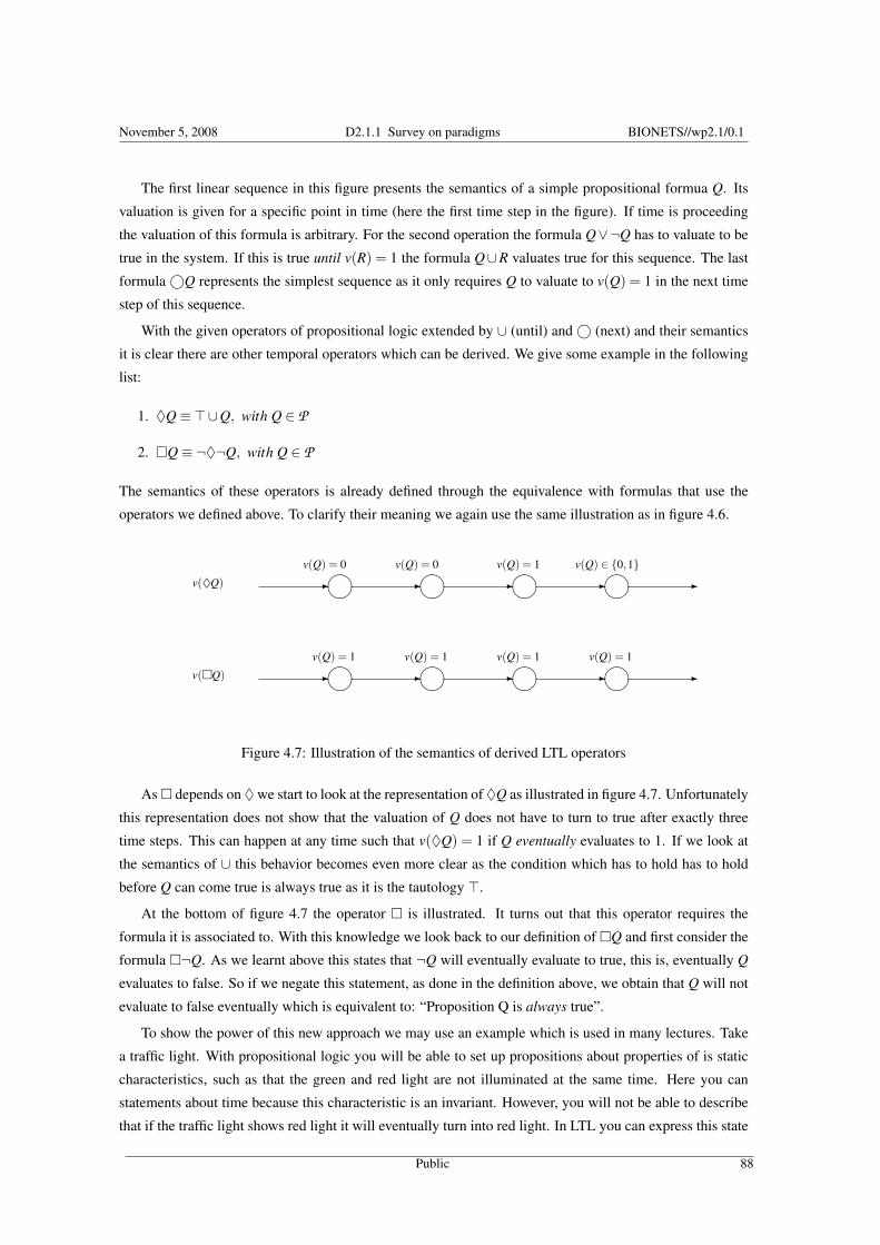
November 5, 2008 D2.1.1 Survey on paradigms BIONETS//wp2.1/0.1
The first linear sequence in this figure presents the semantics of a simple propositional formua Q. Its
valuation is given for a specific point in time (here the first time step in the figure). If time is proceeding
the valuation of this formula is arbitrary. For the second operation the formula Q∨¬Q has to valuate to be
true in the system. If this is true until v(R) = 1 the formula Q∪R valuates true for this sequence. The last
formula ©Q represents the simplest sequence as it only requires Q to valuate to v(Q) = 1 in the next time
step of this sequence.
With the given operators of propositional logic extended by ∪ (until) and © (next) and their semantics
it is clear there are other temporal operators which can be derived. We give some example in the following
list:
1. ♦Q≡>∪Q, with Q ∈ P
2. ¤Q≡ ¬♦¬Q, with Q ∈ P
The semantics of these operators is already defined through the equivalence with formulas that use the
operators we defined above. To clarify their meaning we again use the same illustration as in figure 4.6.
v(¤Q) -v(Q) = 1
±°²¯
-v(Q) = 1
±°²¯
-v(Q) = 1
±°²¯
-v(Q) = 1
±°²¯
-
v(♦Q) -v(Q) = 0
±°²¯
-v(Q) = 0
±°²¯
-v(Q) = 1
±°²¯
-v(Q) ∈ 0,1
±°²¯
-
Figure 4.7: Illustration of the semantics of derived LTL operators
As ¤ depends on ♦ we start to look at the representation of ♦Q as illustrated in figure 4.7. Unfortunately
this representation does not show that the valuation of Q does not have to turn to true after exactly three
time steps. This can happen at any time such that v(♦Q) = 1 if Q eventually evaluates to 1. If we look at
the semantics of ∪ this behavior becomes even more clear as the condition which has to hold has to hold
before Q can come true is always true as it is the tautology >.
At the bottom of figure 4.7 the operator ¤ is illustrated. It turns out that this operator requires the
formula it is associated to. With this knowledge we look back to our definition of ¤Q and first consider the
formula ¤¬Q. As we learnt above this states that ¬Q will eventually evaluate to true, this is, eventually Q
evaluates to false. So if we negate this statement, as done in the definition above, we obtain that Q will not
evaluate to false eventually which is equivalent to: “Proposition Q is always true”.
To show the power of this new approach we may use an example which is used in many lectures. Take
a traffic light. With propositional logic you will be able to set up propositions about properties of is static
characteristics, such as that the green and red light are not illuminated at the same time. Here you can
statements about time because this characteristic is an invariant. However, you will not be able to describe
that if the traffic light shows red light it will eventually turn into red light. In LTL you can express this state
Public 88

November 5, 2008 D2.1.1 Survey on paradigms BIONETS//wp2.1/0.1
change with the formula ¤(R ⊃ ♦G). Here R denotes the proposition “Red light” and G the proposition
“Green light. Reading this formula in natural language yields: It is always true that if there is red light then
eventually there will be green light.
Let us now look at the structure of linear temporal logic. To define it we took a classical propositional
logic and extended it with two additional operators which introduced the time dimension. However, if we
look at the definition of these operators then we could always formulate them with there exists a point in
time or for all points in time. Thus, these definitions suggest themselves to ask whether we could model
linear temporal logic in first order logic.
In fact, it is possible but tedious because we have to model time in first-order logic and thus formulas
become very complex and difficult to read. This is comparable to translating a higher programming lan-
guage to assembler. However, the important result we should remember is that we can model all statements
in propositional temporal logic using first-order logic. In [24] Etessami et al. go even one step further
and prove that unary temporal logic (which is temporal logic with only unary temporal operators as de-
fined above) can be expressed by first-order logic with only two variables. Consequentially, we can use the
algebras developed in the last section to allow the algebraization of unary-temporal logic.
One obvious question follows: Can formulas in first-order temporal logic be translated into first-order
logic and thus is it possible to use the same algebras? The answer to this question would require the
coverage of more theoretical concepts and we would need to extend our discussion of logic to completeness
and other important theories. Therefore, for completeness we mention here that a lot of research has been
conducted in this area. A good overview and introduction can be found in [25] and [26].
Branching Time Logic
So far linear temporal logics have been discussed. They get their name from the fact that they consider only
behaviors which can be modelled as linear time sequences. This characteristic is nicely illustrated by figures
4.6 and 4.7. Every state, represented as a node, has exactly one successor. However, in communication
systems or generally in concurrent systems a state in time will need to have several future states. To model
such system branching time logics [27] have been proposed. They possess tree structure in which each state
in time has more than one successor. One of the most popular of these logics is the computation tree logic
(CTL) proposed in [28].
Although, it is usually easier to model concurrent systems using branching time logic. This is due to
the fact that their additional path quantifiers usually support the navigation in their tree structure. However,
sometimes it easier to use existing tools, proof techniques, and analytical methods which exist already in
one domain. We can state here that branching temporal logics can be translated into linear temporal logic
by simply modelling each branch in the branching logic as a linear sequence in linear temporal logic. This
is common practice when, for example, translating non-deterministic machine models into deterministic
ones.
Applications
In this section we saw how temporal logic can extend classical propositional logic to describe properties of
behavior or generally time-dependent system characteristics.
Public 89

November 5, 2008 D2.1.1 Survey on paradigms BIONETS//wp2.1/0.1
This expressiveness can be used in many different ways. Very popular is the use of various types of
temporal logic in the field of security.
Here the logical formulas are used to describe expected behavior. This behavior could reflect certain
security characteristics of a control flow of a computer program, of a security protocol, or a general access
control mechanism.
Accordingly, the number of application of temporal logic in the field of security is huge.
The following list shows only an overview of areas in which temporal logic is and can be applied and
emphasizes its relevance to security.
Formal Specification has currently a strong focus in many areas of security research. Distributed com-
puting systems, access control and software systems, security protocols, etc. may be subject to using
logic for specifying their security characteristics [29]. This notion of formal verification was mainly
induced by Pnueli [23, 30] and Lamport [31].
Formal Verification One important characteristic of classical and temporal logic is the existence of a proof
calculus which is mainly based on the mathematical foundation of these logics in algebra. This
calculus can be used to show the correctness of system specifications based on logics [30, 31].
Requirements Description Specifiying the security compliant operation of a system does not only require
the thorough specification of its components. It is also required to thoroughly specify how the system
is restricted and what the environment can or can not do. Formulas of (temporal) logic can be used to
specify these requirements.
4.4 Conclusion
The reason we are interested in the metabolism of the cell is that the cell can be considered an immensely
complex parallel computer that executes a ’distributed algorithm’. This term arises from the fact that even
though most of the instructions are coded in the DNA, a significant part of each metabolic cycle depends on
the chemical composition of the cell moment-by-moment. The DNA instructions are propagated through
the cell by diffusion mechanisms coupled with various reactions. The concentrations of the various chemi-
cal species are far from uniform. In addition, several kinds of membranes and structural elements separate
areas of different chemical activities and make the internal topology of the cell nested and extremely com-
plex. There is however an aspect that greatly simplifies the conceptualisation of internal cell operations:
dimensional reduction.
The most successful example of dimensional reduction is provided by the microcanonical ensemble of
equilibrium statistical mechanics: an isolated system will approach equilibrium, which corresponds to the
configuration of highest entropy. The configuration of highest entropy is, by definition, the most probable.
Thus it can be easily identified by the peak in the frequency distribution of all possible configurations. For an
isolated system in equilibrium this is nothing more than the familiar Gaussian, which has a very sharp peak
indeed since it decays on both sides of the maximum like a square exponential. More generally, the Central
Limit Theorem says that a sequence of random samples will converge to a Gaussian for equilibrium systems
[32]. A more detailed discussion of these physics concepts and their relationship to self-organisation can
Public 90
November 5, 2008 D2.1.1 Survey on paradigms BIONETS//wp2.1/0.1
be found in [3]. For our purposes here it is sufficient to recall how the CLT allows the derivation of stable
macroscopic properties such as pressure from the random collisions of O(1023) molecules in a litre of air.
That’s a dimensional reduction of 1023 to 1.
When a gene is activated and begins to signal to the cell machinery to fabricate a particular protein, it
creates several thousand mRNA molecules that set an equal number of ribosomes to work in the cytoplasm
(each cell has millions of ribosomes, or ’protein factories’). Such a large number of proteins will provide a
high probability that the particular function the gene wants to execute will be executed. Therefore, we can
regard the large numbers of molecules in the cell as a strategy to achieve a form of dimensional reduction
that in computer science we generally call ’abstraction’. Several thousand proteins will participate in a
relatively few biochemical reactions to advance one or more metabolic cycles one execution step. Even
though the interior of the cell is never in equilibrium (it relies on its ’fall’ toward equilibrium as the engine
that drives all of its spontaneous self-organising processes—in fact, that’s what ’spontaneous’ means), its
complex topology is divided into many areas in each of which a few reactions are active at any one point
in time. From millions of elements we can therefore see how through a relatively small number of quasi-
equilibrium regions of the cell several hundred metabolic cycles can be executed in parallel.
Dimensional reduction or abstraction working together with the fact that the DNA itself is composed of
genes that can be ON or OFF makes it sound plausible that the internal working of the cell can be modelled
through a discrete or digital framework. We can begin to recognise some of the concepts discussed in
Section 2. For example, the 4 DNA bases represent an alphabet with which the specification of proteins can
be coded. The architecture of the DNA is such that it must not only carry the genetic code but also support
its expression through interactions with its enviroment. This has been achieved by replicating the same
information along the two parallel strands of the DNA molecule, in such a way that the 4 bases are paired
up two-by-two. In other words, of the four bases Thymine (T), Cytosine (C), Adenine (A), and Guanine(G)
[33], only 2 kinds of pairs are possible: A-T and C-G, so that a binary base field might still be relevant in
some way.
Assuming we can recognise an algebraic structure in the digital nature of cell biology, the same or
similar structure would help us make a bridge to the structure of logic. So at this point we may ask the
question: What can we do with logic and biology? As we have explained in Section 4.3.2 it may be
possible that by studying biological systems our research may yield interesting connections between two,
at first sight, completely different domains. However, this is not the final goal of our work.
In BIONETS we are currently exploring characteristics and structure of and operations on Fraglets [34].
They represent a programming model which is based on multi-set rewriting and can be compared to the
copying of DNA sequences described above. In fact, it turns out that the execution model of Fraglets is very
similar to interacting biological systems such as the DNA with the various enzymes that it generates. As
a consequence, one may actually expect that the implementation of genetic algorithms on these structures
may be fairly easy. However, first experiments show that this is not the case. To successfully design
a system which performs genetic operations we need to know what the basic building blocks are with
which we may build new individuals, and which structures of the individual representation (in our case
a program or service) are relevant to yield a ’fit’ individual. We know that biology is very successful in
choosing the right building blocks and the correct genetic operations that are applied to the appropriate
portions of the DNA. By choosing a programming model which is very similar to bio-chemical processes
Public 91
November 5, 2008 D2.1.1 Survey on paradigms BIONETS//wp2.1/0.1
in a cell we hope to be able to transfer the observations made in the realm of biology to a programming
language. In abstract terms, we would like to be able to describe structures of Fraglets using algebra. These
stuctures and their interaction with the environment would correspond to specific program characteristics
and behaviour. This seems possible in principle because we would exploit our observations from biological
system. Here this process is comparable to specific structures of the DNA (genes) which in interaction with
their environment yield different phenotypes of an organism. In this way, Fraglets and their similarity to
bio-chemical processes form the exemplary bridge head of the applicaiton of our theory to security.
As we learnt in this document we can use an algebra and map it into the realm of logic. Depending on
the type of algebra we obtain from the analysis of our programming model we will have the possibility to
analyse the corresponding characteristics in the realm of logic. As explained in section 4.3.3 logic is a pow-
erful means to investigate program properties, including security. Clearly, this process has its limitations as
we will not be able to investigate any arbitrary program characteristic (for example the Halting problem).
However, it will be an important step towards understanding the complicated programming and execution
model of Fraglets and possibly their counterpart in biology, the DNA and its proteins. Furthermore, if we
invert this analytical process, it becomes clear how we could guide evolution. Being able to express specific
program properties in logic, we will be able to express the same characteristic in algebra and thus as a
structure of the programming language, the Fraglets.
Consequently, the insights that we hope to obtain from this bridge between biology and logic could also
help to improve genetic operators. This is due to the fact that it would become easier to investigate the
implications of a structural change (which corresponds to a genetic operation) on the program properties.
Finally, this would also have immediate effect on the design of fitness functions. Based on the knowledge of
which structure of the program representation is responsible for which program property, fitness functions
could be improved. Instead of evaluating program representations as a whole they could analyse their
structure and evaluate only those parts that are relevant for ”survival”. This will also enable better evaluation
of security characteristics of the evolved programs.
The final goal is to be able to specify the security or other functional characteristics of a digital sys-
tem, and have the specifications map to running code through a process analogous to gene expression, i.e.
constructing order through interaction with the environment.
Acknowledgements
The authors would like to acknowledge the valuable feedback they received from Luciana Pelusi and
Marinella Petrocchi on the first draft of this article, and the stimulating conversations they had with Sotiris
Moschoyiannis and Christopher Alm during the course of the research.
The first author would like to acknowledge the partial support of his work by the OPAALS Project,
contract number FP6-034824.
Public 92
Bibliography
[1] S. Kauffman, The Origins of Order: Self-Organisation and Selection in Evolution. Oxford: Oxford
University Press, 1993.
[2] P. Dini, D4.1-DBE Science Vision. www.digital-ecosystem.org, Deliverables: SP0: DBE Project,
2006.
[3] P. Dini and E. Berdou, D18.1-Report on DBE-Specific Use Cases. www.digital-ecosystem.org, De-
liverables: SP5: DBE Project, 2004.
[4] P. Dini, D18.4-Report on self-organisation from a dynamical systems and computer science viewpoint.
www.digital-ecosystem.org, Deliverables: SP5: DBE Project, 2007.
[5] ——, D18.6-5-Year living roadmap for Digital Ecosystems research in biology-inspired computing.
www.digital-ecosystem.org, Deliverables: SP5: DBE Project, 2007.
[6] G. Boole, The Mathematical Analysis of Logic. Bristol: Thoemmes Press, 1998 (1847).
[7] P. R. Halmos, Algebraic Logic. AMS, 2007 (1962).
[8] A. Tarski, Logic, Semantics, Metamathematics. Oxford University Press, 1956, edited by J. H.
Woodger.
[9] L. Henkin, J. D. Monk, and A. Tarski, Cylindric Algebras. Amsterdam: North-Holland, 1971.
[10] P. Cameron, Introduction to Algebra. Oxford: Oxford University Press, 1998.
[11] R. B. J. T. Allenby, Rings, Fields and Groups: An Introduction to Abstract Algebra (2nd Ed.). Oxford:
Butterworth-Heinemann, 1991.
[12] I. Stewart, Galois Theory (2nd Ed.). London: Chapman and Hall, 1989.
[13] J. A. Gordon, “Very simple method to find the minimum polynomial of an arbitrary non-zero element
of a finite field,” Electronics Letters, vol. 12, pp. 663–664, 1976.
[14] M. Fitting, First-order logic and automated theorem proving (2nd ed.). Secaucus, NJ, USA: Springer-
Verlag New York, Inc., 1996.
[15] P. Halmos and S. Givant, Logic as Algebra. Washington, DC: The Mathematical Association of
America, 1998, vol. 21 of Dolciani Mathematical Expositions.
93

November 5, 2008 D2.1.1 Survey on paradigms BIONETS//wp2.1/0.1
[16] C. C. Pinter, “A simple algebra of first order logic,” Notre Dame Journal of Fomal Logic, vol. XIV,
no. 3, July 1973.
[17] B. A. Galler, “Cylindric and polyadic algebras,” in Proceedings of the American Mathematical Society,
vol. 8, no. 1, 1957, pp. 176–183.
[18] P. R. Halmos, “Algebraic logic, i. monadic boolean algebras,” Composito Mathematica, vol. 12, pp.
217–249, 1956.
[19] A. Daigneault, “On automorphisms of polyadic algebras,” Transactions of the American Mathematical
Society, vol. 112, no. 1, pp. 84–130, 1964.
[20] M. Krasner, “Généralisation abstraite de la théorie de galois,” in Algèbre et théorie des nombres, ser.
C.N.R.S. Paris: Centre national de la Recherche scientifique, 1950, no. 24, pp. 163–168.
[21] H. Andréka, I. Németic, and J. Madarász, “On the logical structure of relativity theories.” Electroni-
cally available at http://www.math-inst.hu/pub/algebraic-logic/Contents.html, Tech. Rep., 2002.
[22] H. Andréka, J. X. Madarász, and I. Németi, “Algebras of relations of various ranks, some current
trends and applications,” JoRMiCS, vol. 1, pp. 27–49, 2004.
[23] A. Pnueli, “The temporal logic of programs,” in Proceedings of the 18th IEEE Symposium on Foun-
dations of Computer Science, 1977, pp. 46–57.
[24] K. Etessami, M. Y. Vardi, and T. Wilke, “First-order logic with two variables and unary temporal
logic,” Information and Computation, vol. 179, no. 2, pp. 279–295, December 2002. [Online].
Available: http://dx.doi.org/10.1006/inco.2001.2953
[25] M. Gehrke and Y. Venema, Algebraic Tools for Modal Logic. Electronically available at
http://www.helsinki.fi/esslli/courses/readers/K15.pdf, Helsinki, Finland: European Summer School
in Logic, Language and Information, 2001.
[26] P. Blackburn, M. de Rijke, and Y. Venema, Modal Logic. Cambridge University Press, 2001.
[27] M. Ben-Ari, Z. Manna, and A. Pnueli, “The temporal logic of branching time,” in POPL ’81: Pro-
ceedings of the 8th ACM SIGPLAN-SIGACT symposium on Principles of programming languages.
New York, NY, USA: ACM Press, 1981, pp. 164–176.
[28] E. M. Clarke, E. A. Emerson, and A. P. Sistla, “Automatic verification of finite state concurrent system
using temporal logic specifications: a practical approach,” in POPL ’83: Proceedings of the 10th ACM
SIGACT-SIGPLAN symposium on Principles of programming languages. New York, NY, USA: ACM
Press, 1983, pp. 117–126.
[29] F. Kröger, Temporal logic of programs. New York, NY, USA: Springer-Verlag New York, Inc., 1987.
[30] Z. Manna and A. Pnueli, The temporal logic of reactive and concurrent systems. New York, NY,
USA: Springer-Verlag New York, Inc., 1992.
Public 94
November 5, 2008 D2.1.1 Survey on paradigms BIONETS//wp2.1/0.1
[31] L. Lamport, “The temporal logic of actions,” ACM Transactions on Programming Languages
and Systems, vol. 16, no. 3, pp. 872–923, May 1994. [Online]. Available: citeseer.ist.psu.edu/
lamport94temporal.html
[32] D. Sornette, Critical Phenomena in Natural Sciences: Chaos, Fractals, Self-organization and Disor-
der - Concepts and Tools. Heidelberg: Springer, 2000.
[33] B. Alberts, A. Johnson, J. Lewis, M. Raff, K. Roberts, and P. Walter, Molecular Biology of the Cell
(4th Ed.). New York: Garland Science, 2002.
[34] C. Tschudin, “Fraglets - a metabolistic execution model for communication protocols,” in 2nd Annual
Symposium on Autonomous Intelligent Networks and Systems (AINS), Menlo Park, USA, July 2003.
[35] R. Sanchez, E. Morgado, R. Grau, “Gene algebra from a genetic code algebraic structure”, Journal of
Mathematical Biology, 51, 431-457 (2005).
Public 95

November 5, 2008 D2.1.1 Survey on paradigms BIONETS//wp2.1/0.1
Public 96
Chapter 5
Evolutionary Computing and ArtificialEmbryogenyL. Yamamoto, D. Miorandi
Abstract. In this chapter we present a review of state-of-the-art techniques for automated creation and evolution of
software. The focus is on bio-inspired bottom-up approaches, in which complexity is grown from interactions among
simpler units. First, we review Evolutionary Computing (EC) techniques, highlighting their potential application to
the automated optimization of computer programs in an online, dynamic environment. Then, we survey approaches
inspired by embryology, in which artificial entities undergo a developmental process. The chapter concludes with a
critical discussion and outlook for applications of the aforementioned techniques to the BIONETS environment.
5.1 Introduction
Building software that is able to continuously improve itself automatically is a common goal in artificial in-
telligence, software engineering, and other areas of computer science, including, more recently, autonomic
systems and organic computing. The dream is to bring to computers the ability to constantly seek to learn
and adapt, driven by a concrete purpose and motivation coming from the interaction with the real world
[38].
Efforts in this direction follow a top-down or a bottom-up approach: Top-down approaches attempt to
automate the reasoning process used in software engineering and design, from user requirements down to
the code implementation. These include automatic program and protocol synthesis from specifications [27,
36] and more recently, derivation of policy rules from high-level representations closer to natural language
[51, 47]. Bottom-up approaches look at how higher-level software functionality would emerge from lower-
level interactions among simpler system units. Artificial Life (ALife), Evolutionary Computation, Swarm
Intelligence and other areas focus on such bottom-up approach.
While the top-down approach seeks a formal model of software construction by humans, the bottom-
up approach is essentially biologically-inspired. Even the most elementary life forms possess a level of
robustness and adaptation far beyond current artificial systems, therefore it seems worthwhile to learn from
biology in order to draw inspiration for the design of new systems.
97
November 5, 2008 D2.1.1 Survey on paradigms BIONETS//wp2.1/0.1
In this chapter we provide a survey of bio-inspired approaches to such bottom-up creation of software
functionality. Our focus is on dynamic, online processes where evolution and adaptation must happen con-
tinuously, during the operation of the system, as opposed to off-line, design-time optimization approaches.
We investigate the potential of bio-inspired algorithms to obtain systems that are able to continuously pursue
an optimum operation point without ever stopping. Such online optimization process involves the ability to
self-organize into structures at multiple scales, analogous to cells, multicellular organisms, up to artificial
ecosystems of interacting parts.
Numerous bio-inspired systems are available. A classification was proposed in [41], which positions
them in a 3-D space defined by three axes, related to evolution of functionality, structural growth, and learn-
ing ability, respectively. We focus on the first two axes, represented mainly by evolutionary computation
and developmental approaches related to embryology.
This chapter is organized as follows. In Sec. 5.2 we position our context within the classification adopted
from [41]. In Sec. 5.3 we review the state-of-the-art in evolutionary computing with focus on online and
dynamic environments. In Sec. 5.4 we present the two main research lines inspired by embryology: embry-
onics and artificial embryogenies. Sec. 5.5 presents a critical discussion on the possible combination of the
aforementioned approaches. Sec. 5.6 concludes the chapter pointing out possible applications to BIONETS.
5.2 Context: The PO-Plane
A classification of bio-inspired systems was proposed in [41], positioning them in a 3-D space defined by
three orthogonal axes. Although it was proposed ten years ago for hardware, its concepts remain valid today,
and apply to software as well. We focus on two of the the three axes, namely Phylogeny and Ontogeny. The
third axis (Epigenesis), related to learning, covers techniques such as artificial neural networks and artificial
immune systems, which are outside the scope of the present survey. The two remaining axes are defined as
follows:
• Phylogeny or phylogenesis is the process of genetic evolution of species. Phylogenetic mechanisms
are essentially non-deterministic, with mutation and recombination as major variation triggers. Arti-
ficial systems along this axis perform Artificial Evolution (AE) either in hardware (Evolvable Hard-
ware) or in software (Evolutionary Computation). The latter will be described in Section 5.3.
• Ontogeny or ontogenesis is the process of growth and development of a multicellular organism from
the fertilized egg to its mature form. Ontogeny is studied in developmental biology, which covers
the genetic control mechanisms of cell growth, differentiation and morphogenesis. Artificial systems
here go from simple replicators and self-reproducing systems to embryonics (mostly in hardware)
and artificial embryogeny (mostly in software). These will be described in Section 5.4.
The POE classification is represented in Fig. 5.1, where some of the techniques which will be treated in
this paper are positioned on the PO-Plane.
As predicted in [41], today combinations of both approaches, forming the so-called PO-Plane, are be-
coming more and more common. On one hand, an indirect encoding followed by a developmental process
has shown to increase the scalability of evolutionary computing for complex problems. On the other hand,
Public 98
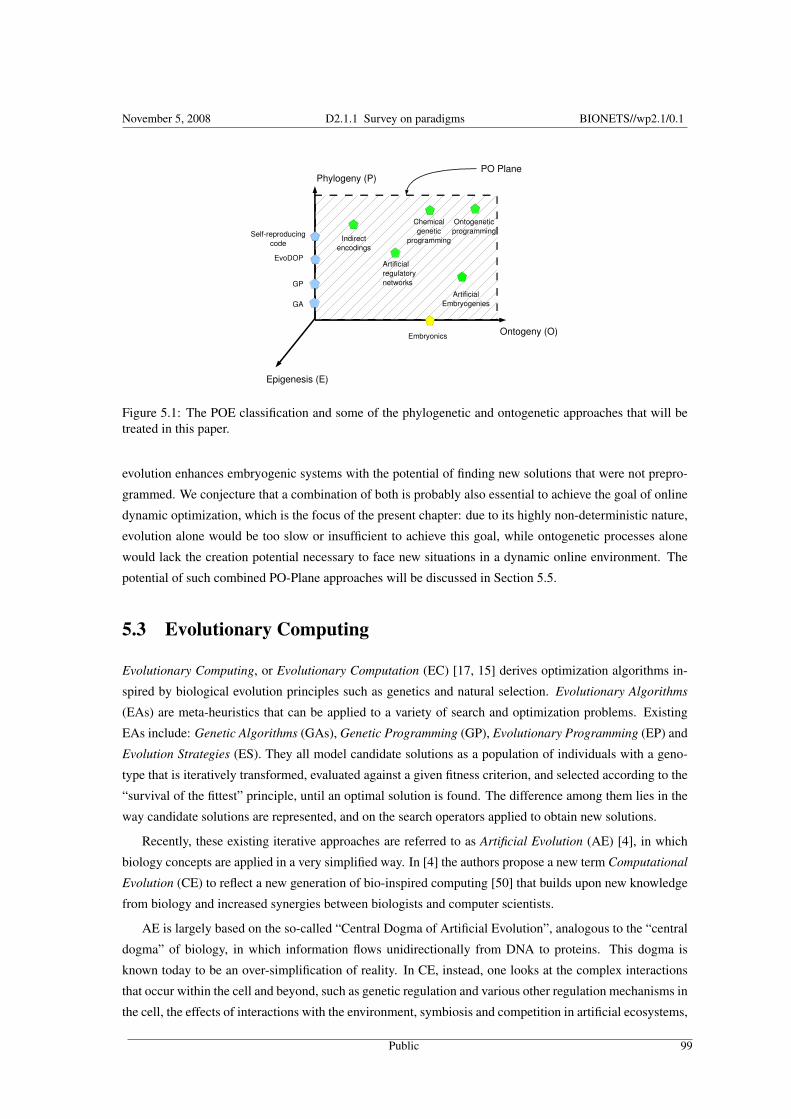
November 5, 2008 D2.1.1 Survey on paradigms BIONETS//wp2.1/0.1
Figure 5.1: The POE classification and some of the phylogenetic and ontogenetic approaches that will betreated in this paper.
evolution enhances embryogenic systems with the potential of finding new solutions that were not prepro-
grammed. We conjecture that a combination of both is probably also essential to achieve the goal of online
dynamic optimization, which is the focus of the present chapter: due to its highly non-deterministic nature,
evolution alone would be too slow or insufficient to achieve this goal, while ontogenetic processes alone
would lack the creation potential necessary to face new situations in a dynamic online environment. The
potential of such combined PO-Plane approaches will be discussed in Section 5.5.
5.3 Evolutionary Computing
Evolutionary Computing, or Evolutionary Computation (EC) [17, 15] derives optimization algorithms in-
spired by biological evolution principles such as genetics and natural selection. Evolutionary Algorithms
(EAs) are meta-heuristics that can be applied to a variety of search and optimization problems. Existing
EAs include: Genetic Algorithms (GAs), Genetic Programming (GP), Evolutionary Programming (EP) and
Evolution Strategies (ES). They all model candidate solutions as a population of individuals with a geno-
type that is iteratively transformed, evaluated against a given fitness criterion, and selected according to the
“survival of the fittest” principle, until an optimal solution is found. The difference among them lies in the
way candidate solutions are represented, and on the search operators applied to obtain new solutions.
Recently, these existing iterative approaches are referred to as Artificial Evolution (AE) [4], in which
biology concepts are applied in a very simplified way. In [4] the authors propose a new term Computational
Evolution (CE) to reflect a new generation of bio-inspired computing [50] that builds upon new knowledge
from biology and increased synergies between biologists and computer scientists.
AE is largely based on the so-called “Central Dogma of Artificial Evolution”, analogous to the “central
dogma” of biology, in which information flows unidirectionally from DNA to proteins. This dogma is
known today to be an over-simplification of reality. In CE, instead, one looks at the complex interactions
that occur within the cell and beyond, such as genetic regulation and various other regulation mechanisms in
the cell, the effects of interactions with the environment, symbiosis and competition in artificial ecosystems,
Public 99

November 5, 2008 D2.1.1 Survey on paradigms BIONETS//wp2.1/0.1
and other highly dynamic processes which occur in many real-life problems. CE is of particular interest in
online dynamic scenarios which are the focus of this survey. Note that there is no clear-cut border between
AE and CE, but rather a gradual transition. For instance, the combination of phylogenetic and ontogenetic
mechanisms positioned on the PO-Plane can be seen as a movement in the CE direction.
5.3.1 Genetic Algorithms
In a Genetic Algorithm (GA) [19] candidate solutions are represented as a population of individuals whose
genotype is a string of solution elements (bits, characters, symbols, etc.). Strings typically have a fixed
or bounded length, such that the size of the search space can be constrained. The goal of a GA is to
find the optimum value of such string that optimises a given fitness criterion. An initial population of
candidate strings is generated and evaluated against the fitness criterion. Multiple candidate solutions are
then chosen (usually with a probability which depends on the respective fitness level) for giving rise to the
next generation. This is accomplished by applying genetic operators (e.g., crossover and mutation) to such
candidate solutions in order to create new variants.
5.3.2 Genetic Programming
Genetic Programming (GP) [21, 6, 24] applies the GA idea to evolve computer programs automatically. A
GP algorithm is essentially the same as a GA, but the candidate solutions encode computer programs, such
that they can solve all instances of a problem, instead of optimizing for a particular instance as in GA.
GP typically evolves programs encoded in a linear (similar to assembly language) or tree representation
(similar to functional languages such as LISP). Other representations are also possible, such as graphs
[35, 29], finite state machines [1, 40, 39], neural networks [30], and more recently, chemical programs
[28, 54].
When solving a problem by GP, one generally does not know the maximum size of the target solution
program. Therefore, the genotype representation in GP generally allows for variable-length programs with
unbounded size. The size of the search space in this case is infinite, so programs can in principle grow
indefinitely. The bloat phenomenon was discovered early in the GP history, and refers to the fact that pro-
grams evolved by GP (especially tree-based GP) tend indeed to grow very large, with obvious shortcomings
in terms of memory usage and execution efficiency. The bloat phenomenon is generally accompanied by
an intron growth phenomenon, in which non-coding regions emerge, that have no effect on the program
outcome. Although some authors pointed out that this phenomenon may also have positive effects, such as
some protection against destructive crossover, it was mandatory to control code growth. Several methods
were proposed for this purpose, such as parsimony pressure [26].
Recently, special attention has been devoted to indirect representations in which a genotype encoding
is mapped onto a different phenotype representation. The goal is make GP solutions scale to complex
problems without corresponding growth in program size. Indirect encodings may also provide additional
robustness and evolvability, via redundant representations in which one phenotype may be expressed by
more than one genotype, and via neutrality in representations, in which mutations in the genotype do not
immediately affect the corresponding phenotype. This is especially important for online evolution. Indirect
encodings will be briefly discussed in Section 5.3.6.
Public 100

November 5, 2008 D2.1.1 Survey on paradigms BIONETS//wp2.1/0.1
Most GP approaches can be placed along the “P” axis in the POE framework (Fig. 5.1). Some indirect
encodings include a growth process which positions them on the PO-plane. An example is an Artificial
Embryogeny, which will be discussed in Section 5.4.2.
5.3.3 Evolutionary Computing for Dynamic Optimization
EC techniques have been widely used for solving optimization problems in dynamic environments, in which
the problem instance or the constraints may vary over time[20]. The aim is to introduce mechanisms able to
“track” the optimal solution. This field is referred to as Evolutionary Computing for Dynamic Optimization
Problems (EvoDOP). EC provides a natural framework for dynamic optimization, in that natural evolution
is a continuous process. Most approaches in EC for dynamic optimization are based on the assumption that
the changes in the problem settings are gradual, such that the previous population can be reused to search
for the new optimum, without having to restart from scratch.
One of the main problems in EvoDOP is premature convergence: the population quickly converges
to the optimum and tends to become very uniform, i.e. all solutions resemble the best one. In a static
environment this is not an issue, since one can stop searching once a satisfactory solution is found. In a
dynamic environment, premature convergence hinders the ability to search for new solutions. Proposed
solutions for this problem include:
• Generate diversity after a change, e.g. through Hypermutation, i.e. artificially high mutation rates in
response to a change.
• Maintain diversity throughout the run, e.g. through random immigrants, individuals that move be-
tween subpopulations.
• Implicit memory: usually takes the form of a redundant representation such as diploid or polyploid
individuals with a dominance mechanism.
• Explicit memory: previously good solutions are stored in memory, and retrieved when the system
encounters a previous situation for which the solution applied.
• Multi-population: Different subpopulations are spawned from a main population and assigned a sub-
space in which to track local optima. Several different promising subspaces can then be explored
simultaneously.
• Anticipation and prediction: These are recent methods that attempt to predict the consequences of
current decisions on the future of the system, such that informed decisions can be taken which will
lead to improved results with high probability [8].
Although much has been done in EvoDOP in the GA domain, little has been explored in the GP do-
main. In [11] the authors show a multi-chromosome approach to GP based on Prolog programs. Multi-
chromosomal GP is a polyploidy mechanism, thus a variant of implicit memory, which has been shown to
achieve only mitigated results in EvoDOP. Indeed, the approach [11] is not applied to a dynamic environ-
ment. In nature, however, polyploidy mechanisms are extremely helpful, therefore it would be interesting
Public 101
November 5, 2008 D2.1.1 Survey on paradigms BIONETS//wp2.1/0.1
to see how to improve the analogous artificial mechanisms to achieve an equivalent performance. An-
other research line would be to bring the most promising EvoDOP approaches to the GP domain, namely
multi-population and anticipation. EvoDOP techniques are mainly situated along the “P” axis in the POE
framework.
5.3.4 Self-Replicating and Self-Reproducing Code
Much attention has been paid in EC on self-replicating and self-reproducing code. In some cases, replication
and reproduction have actually been considered synonymous, which they are not [41]. Replication is an
ontogenetic, developmental process, involving no genetic operators, resulting in an exact duplicate of the
parent organism. Reproduction, on the other hand, is a phylogenetic (evolutionary) process, involving
genetic operators such as crossover and mutation, thereby giving rise to variety and ultimately to evolution.
The study of self-replicating software can be traced back to the pioneering work of John von Neumann
in the late 40s on self-replicating automata. He set the basis for a mathematically rigorous study of self-
replicating artificial machines based on cellular automata. Since then, several examples of self-replicating
machines have been shown and elaborated [18]. Such machines are able to produce an identical copy of
themselves, which means that the copy must also contain the part of the code that is able to produce a further
copy of itself. Errors in the replication process are usually not allowed, and recovery from copy errors are
thus in general not provided.
Self-reproducing code, on the other hand, involves a variation mechanism by which the new individual
is not an exact copy of its parent. Self-reproduction thus requires some form of self-modification, which
will be discussed below. Moreover it must include resilience to harmful replication errors in the form of a
self-repair mechanism, or a selection mechanism able to detect and discard harmful code.
5.3.5 Self-Modifying Code
In a system that is required to constantly evolve and adapt, the ability to automatically modify or update its
own code parts is essential. Since reliable and secure self-modification is still an open issue, self-modifying
code has been banished from good practice software engineering.
However, self-modifying code plays a key role in EC and ALife, where evolution still occurs mostly in
a simulated environment. In the case of EC, only the best programs which have been thoroughly tested via
multiple fitness cases can be safely used. In the case of ALife, the main role of programs is just to survive,
and since they remain in a virtual world there is no risk for the end user.
Evolvable instruction set virtual machines are used in most well-known ALife systems, such as Tierra
and Avida. They resemble assembly language, which is easily self-modifiable: one can write on memory
positions that include the own memory location of the code. This is used to evolve software that self-
reproduces, adapts, seeks to survive, etc. A precursor of such machine language approach was Core Wars
[13].
In the GP context, the Push family of programming languages [42] is designed for a stack-based virtual
machine in which code can be pushed to a stack and therefore be manipulated as data. A variant of Push
was used in Autoconstructive Evolution [43], where individuals take care of their own reproduction, and the
reproduction mechanism itself can evolve (showing self-modification at the level of reproduction strategies).
Public 102
November 5, 2008 D2.1.1 Survey on paradigms BIONETS//wp2.1/0.1
Recently [42], an enhancement of the language permitting the explicit manipulation of an execution stack
has been introduced. It has been shown to evolve iterative and recursive function which are non-trivial to
be evolved in GP.
Ontogenetic Programming [45] is a developmental approach to GP in which the generated programs
include self-modification instructions that enable them to change during the run. This is foreseen as an
advantage for adaptation to the environment. To illustrate the concept, in [44] Ontogenetic Programming is
applied to a virtual world game in which agents must find gold and survive multiple dangers and obstacles.
It is shown that the ontogenetic version is able to evolve correct solutions to the game, where traditional GP
fails to do so. This is an interesting example of hybrid approach located along the PO-Plane.
5.3.6 Indirect Encodings in Evolutionary Computing
It is well known in Evolutionary Computing that the representation of candidate solutions and the genetic
operators applied to it play a key role in the performance of the evolutionary process. The genotype to
phenotype mapping scheme is included in this representation problem, and it is well known in GP that
indirect encodings like Cartesian GP [29] and Grammatical Evolution [31] can greatly help in obtaining
viable individuals. Moreover they present a potential for encoding neutrality.
Neutrality occurs when small mutations in the genotype are likely not to affect the fitness of the cor-
responding individual. Such “silent” mutations, which modify the genotype while leaving the fitness un-
changed, are called neutral mutations. Since the resulting changes are not subject to selection, their imme-
diate impact is invisible. At first sight, they slow down evolution. However, over the long run, as neutral
mutations accumulate, some genotypes may end up expressing a different solution with a potentially higher
fitness. Neutrality provides a “smooth” way to explore the search space, and has been shown to potentially
increase the evolvability of a population.
Indirect encodings may also be used to enhance the scalability of EC to complex problems: a compact
genotype can express a large number of different phenotypes, such that the number of genes required to
specify a phenotype may be orders of magnitude less than the number of structural units composing the
phenotype. If coupled with developmental approaches (embryogeny, morphogenesis) it can encode pheno-
types that grow from simple structures to more complex ones.
Many indirect encoding approaches include such a developmental process and can therefore be posi-
tioned on the PO-plane of the POE framework.
5.3.7 Approaches Based on Gene Expression
Many indirect encoding approaches have taken inspiration from gene expression in order to improve the
performance of EC, especially GP. In these approaches, the process of decoding a genotype into a phenotype
is analogous to expressing genes, and is controlled by a regulation or feedback mechanism.
Artificial Regulatory Networks have been shown to model the biological regulatory mechanisms in
both natural [25] and artificial systems [23]. In [25] a genetic network exhibiting stochastic dynamics is
evolved using a set-based encoding of systems of biochemical reactions. In [23] the regulatory network
is represented with a genotype/phenotype binary encoding in which genes express proteins, which in turn
Public 103
November 5, 2008 D2.1.1 Survey on paradigms BIONETS//wp2.1/0.1
control the expression of genes, unleashing large reaction networks that evolve by gene duplication and
mutations. These networks are able to compute functions, such as a sigmoid and a decaying exponential.
Chemical Genetic Programming [34] proposes a feedback-based dynamic genotype to phenotype trans-
lation mechanism inspired by a cell’s dual step transcription-translation process from DNA to proteins.
Using a chemical reaction mechanism, it dynamically builds the rewriting rules of a grammar used to trans-
late a linear genotype into a tree phenotype. This leads to a highly dynamic and evolutive genotype to
phenotype mapping: starting from a pool of simple grammar rules, the system evolves more complex ones
and discards those that are not useful. While the concept itself seems promising, the encoding used and the
algorithm itself are relatively complex, albeit applied to relatively simple problems.
Epigenetic Programming [48] associates a developmental process to GP, in which an Epigenetic Learn-
ing (EL) algorithm activates or silences certain parts of the genetic code. This is said to protect individuals
from destructive crossover by silencing certain genotypic combinations and explicitly activating them only
when they lead to beneficial phenotypic traits. The authors show a 2-fold improvement in computational
effort with respect to GP, on a predator-prey pursuit problem. Although in this approach a potentially large
number of phenotypes can be expressed from a single genotype, this apparent increase in complexity is
misleading, since all phenotypes are subsets of the original genotype.
Gene Expression Programming (GEP) [16] uses a linear genotype representation in the form of a chro-
mosome with multiple genes. Each gene is translated into an expression tree, and trees are connected
together by a linking function. Although inspired by gene expression, this approach does not include any
dynamic feedback mechanism.
5.3.8 Chemical Computing Models and Evolution
Chemical computing models [3, 10, 33, 14] express computations as chemical reactions that consume and
produce computation objects (data or code). Objects are represented as elements in a multiset, an unordered
set within which elements may occur more than one. The number of occurrences of a given element within
the multiset is called the multiplicity of the element.
We believe that chemical models have a great potential for the class of online dynamic software opti-
mization problems that we are aiming at. This is due to their inherent parallelism and multiset model, which
permits several copies of instructions to be present simultaneously. We conjecture that a chemical language
can express programs that can be more easily transformed and can become more robust to disruptions due
to alternative execution paths enabled by a multiset model.
In this section we discuss some work in evolving programs using a chemical representation, which
presents a new challenge for GP.
An Algorithmic Chemistry [5, 52] is a reaction vessel in which instructions are executed in random
order. In [5] the power of GP applied to an algorithmic chemistry on evolving solutions specific problems is
shown. The authors point out the importance of the concentration of instructions, rather than their sequence.
They start from a nearly unpredictable system in which execution of instructions at a random order leads
to a random program output. This system is set to evolve by GP, including crossover and mutation of
instructions placed in registers. After some generations, some order can be observed, and at the end of the
evolutionary process a highly reproducible output is obtained, in spite of the random execution order.
Public 104
November 5, 2008 D2.1.1 Survey on paradigms BIONETS//wp2.1/0.1
The emergence of evolution in a chemical computing system is investigated in [28], using organiza-
tion theory. Artificial biochemical signaling networks are evolved in [12] to compute several mathematical
functions, using an evolutionary computation method based on asexual reproduction and mutations. Al-
though the networks evolved in [12] show computational capacity, it does not seem trivial to extend their
capabilities from mathematical functions to generic software actions.
We are working on our own chemical programming language [54, 53] which we are extending with
generic computation capacity and an evolution framework in which evolution will occur in an intrinsic and
asynchronous manner as in nature. Variation operations such as mutation and recombination will occur
within the individuals themselves as self-modifying code.
With such chemical systems it becomes possible to quantitatively regulate the behaviour of programs
for evolution or adaptation purposes. An example of that is Chorus [2], a grammar-based GP system which
uses a concentration table to keep track of concentrations of rules in the system. The rule with the highest
concentration is picked for execution. The purpose is to obtain a system in which the absolute position of
a gene (encoding a grammar rule number) does not matter. Such a system is then more resilient to genetic
operators. In [53] we have proposed a code regulation system based on the control of the concentration
of signals that activate or inhibit the expression of given genotypes according to their fitness. While [2]
chooses the rule with the highest concentration, in [53] the choice is probabilistic: the chance of a variant
being picked for execution is proportional to the concentration of its expression signals. While [53] is
explicitly intended for online problems, to the best of our knowledge[2] has not been applied in this context.
5.4 Embryology
Embryology, in general, is a branch of developmental biology focusing on embryogeny, i.e., the process by
which the embryo is formed and develops, from fertilization to mitotic divisions and cellular differentiation.
The ability of embryos to generate complexity starting from a basic entity has generated a lot of attention
in the computing field, since the ability to replicate in silico such process would enable researchers to break
the complexity ceiling which limits the ability of conventional EC techniques.
The application of ideas from embryology (or, better: embryogenies) to artificial systems has been
following two main research directions. One is embryonics (embryology plus electronics), an approach to
improve fault tolerance in evolvable hardware by using a cellular architecture presenting dynamic self-repair
and reproduction properties. Another one is artificial embryogeny, which aims at extending evolutionary
computing with a developmental process inspired by embryo growth and cell differentiation, such that
relatively simple genotypes with a compact representation may express a wide range of phenotypes or
behaviors. These two directions reflect just different communities (hardware vs. software) rather than a
clear conceptual partition, since the underlying concepts are common to both. Indeed, embryonics can be
considered as a branch of artificial embryogeny which focuses on cell differentiation as an error handling
mechanism in reconfigurable hardware, without necessarily covering evolutionary aspects.
5.4.1 Embryonics
The main goal of embryonics [9, 37, 32, 49] is to embed extreme fault tolerance into electronic devices (e.g.,
FPGA arrays) while maintaining the redundancy (e.g., number of “spare” columns/rows in FPGA arrays) at
Public 105
November 5, 2008 D2.1.1 Survey on paradigms BIONETS//wp2.1/0.1
acceptable levels. Approaches in this area have mostly focused on the use of artificial stem cells, i.e., cells
which are able to differentiate into any specific kind of cell required for the organism to work. The approach
is based on the flexibility offered by embryology-based mechanisms, in which there is no need to specify
a priori the actions to be undertaken as a consequence of a fault detected. In FPGA arrays, specifying the
reaction to each possible fault configuration would lead to poorly scalable designs, while at the same time
resulting in a large overhead, due to the need of maintaining a large number of spare rows/columns. The
systems devised in embryonics are based on the following two principles:
• Each cell (understood as the smallest indivisible building block of the system) contains the whole
genome, i.e., has the complete set of rules necessary for the organism to work. Each cell is totipotent,
i.e., can differentiate into any specific function and decides, based on the interaction with neighboring
cells, which functionalities (genes) need to be expressed.
• The system possesses self-organizing properties. Each cell monitors its neighborhood and, upon
detection of a faulty component, can return to the stem cell state and differentiate into another type
of cell to repair the fault. (Some works have proposed to use solutions inspired by the mammalian
immune system to implement this second functionality [9].) This step involves the availability of
“spare” cells, which provide resources necessary to replace the faulty component.
The main difference between the embryonics approach to fault tolerance and classical approaches is that
classical fault tolerance techniques tend to focus on simple replication as a way to achieve redundancy that
can be used to recover from failures. In embryonics the information stored in neighboring cells that might
have differentiated to perform other functions may be used to recreate a lost functionality by re-expressing
the corresponding genes that may be dormant in other cells. Such flexibility to switch functionality adds
another level of robustness, as now not only cells with identical functionality can be used as backup or
template to repair a failure, but also other cells with different functionalities can be used to recreate a lost
one. In evolvable hardware, functionality is mainly expressed by the state of a cell (e.g. in the form of
a configuration register), while in software it could also take the form of a computer program. Let us, for
example, consider a distributed service, i.e., a service whose outcome comes from the interaction of different
components running on different machines. Distributed services are prone to errors related to the possible
faults of one (or more) of the machines where the components reside and run. This is particularly important
in open uncontrolled environments, where the resources used for providing the service do not reside on
dedicated servers but are the spare resources possibly present in user’s desktop or even mobile devices. A
reactive and efficient self-repair or self-healing ability is essential in this context. It is not enough to rely
purely on classical fault tolerance, where failure modes must be pre-engineered into the system. Neither
can we rely exclusively on evolutionary mechanisms, which tend to be slow and unreliable, requiring a
resilience mechanism of their own. Clearly, embryonics provides a middle ground in which diversity can
be exploited for quick repair and re-adaptation, without changing the underlying (potentially evolvable)
genotype. This will involve the construction of artificial stem cells, in the form of representation of the
complete service instructions to be used. Such artificial stem cells shall be spread in the network, where
they shall differentiate (for example following a reaction-diffusion pattern) into the different components
needed for performing the service. Upon detection of a fault, they could re-enter the embryo state, for
differentiating again into the required functionalities, expressing the necessary genes.
Public 106

November 5, 2008 D2.1.1 Survey on paradigms BIONETS//wp2.1/0.1
The Embryonics approach does not encompass any evolutionary aspect. Therefore, in terms of the
classification introduced in Sec. 5.2, we can position it as a pure ontogenetic approach.
5.4.2 Artificial Embryogeny
Artificial Embryogeny [46] is a branch of Evolutionary Computing (EC) in which compact genotypes are
expressed into phenotypes that go through a developmental phase that may cause them to differentiate to
perform specific functions. Indeed, researchers have recognized that “conventional” EC techniques (like
GA, GP, Evolutionary Strategies, etc.) present scalability problems when dealing with problems of relevant
complexity [17]. The issue is that the size of the genotype representing possible solutions in the search
space turns out to grow fast as the complexity of the organism/behavior to be optimized grows. One solution
studied in such approach has been to add one more level of abstraction. In such case, the genotype does
not code the solution itself, but it codes recipes for building solutions (i.e., phenotypes). In this way, a
genotype change does not imply a direct change in the solution, but in the way solutions are decoded from
the genotype and further grown from an initial “seed” (the embryo).
In the case of GP, such indirect genotype encodings play an important role in obtaining viable indi-
viduals (i.e., syntactically correct programs suitable to be executed) via genetic transformations such as
crossover and mutation. Approaches in the GP area are classified according to the genotype representa-
tion and decoding: grammatical evolution and developmental/ontogenetic GP [17]. In the first case, the
genotype is a grammar that comprises a set of rewriting rules which are applied until a complete phe-
notype is obtained [31]. Since grammar production rules are applied to obtain the program, the derived
program is syntactically correct by construction. In the second case, the genotype contains a set of instruc-
tions/transformations which are applied repeatedly on an embryonic entity to obtain a full organism. One
of the most prominent examples of the second case is Ontogenetic Programming [45] (see Section 5.3.5),
which produces self-modifying programs that are highly adaptive.
Note that although grammatical evolution is an indirect encoding approach, it is not performing em-
bryogeny per se, as the generated individuals do not necessarily continue to develop after the phenotype
is expressed. One could easily imagine a grammar to express self-modifying programs (for instance, a
grammar that encodes for the stack-based linear programs in [45, 44]) such that grammatical evolution then
becomes part of the full cycle of evolution, gene expression, development and adaptation. However this is
orthogonal to the developmental process implied in artificial embryogeny.
Other grammar approaches outside the GP context have an inherent growth model which has been as-
sociated with artificial embryogeny. Chapter 2.1 of [46] presents a survey of these grammatical approaches
to artificial embryogeny. A simple one is to use L-Systems. L-Systems, or Lindenmayer Systems, express
fractal-like objects using a grammar where the production rules may or may not contain parameters that
determine how the structure will grow. Why is this form of grammar closer to embryogeny than grammat-
ical evolution? Since L-Systems encode structures as opposed to executable programs, any intermediate
step in the expansion of an L-System is a valid structure (thus a valid individual in growth process), while
in grammatical evolution the first valid program that can be executed is one in which all production sym-
bols (non-terminals) have been rewritten into terminal ones. On the other hand, L-Systems have not been
designed with evolution in mind, although they have been later used for this purpose.
Public 107
November 5, 2008 D2.1.1 Survey on paradigms BIONETS//wp2.1/0.1
Studies on artificial embryogeny [7] have reported a clear advantage of an indirect encoding over a di-
rect one such as tree-based GP. On the other hand, further experiments [22] report that the indirect approach
actually takes much longer to run, and show cases where tree-based GP outperforms the indirect approach
and vice-versa. What remains consistent across different experiments is that in general, indirect encodings
perform best when the problem is complex. There is therefore a trade-off between the computational re-
sources needed for performing embryogeny and the complexity of the problem to be tackled, which needs
to be carefully accounted for, especially in the presence of resource-constrained devices.
Artificial embryogenies may encompass both an ontogenetic as well as a phylogenetic aspect: as such,
they lie in the PO–plane.
5.5 Discussion: EC and Embryology: Common Synergies
While Evolutionary Computing and Embryology-based approaches pertain both —broadly speaking— to
the same research area, and while there is a considerable overlap in the research communities involved
(with the notable exception of embryonics), there are many synergies which have not been exploited so far.
Indeed, embryology-based approaches are still in their infancy, having been mostly applied to solve simple
problems or toy–cases, and could profit from the 30+-years experience and insight gained from research
in EC. At the same time, it is worth remarking that a thorough understanding of all the combinations
possible on the PO-Plane is still missing. Nonetheless, embryology–based approaches have the potential
to complement genetic-based EC techniques by providing a different level of system dynamics. While,
indeed, one of the advantages of artificial embryogenies is related to the possibility of encoding complex
behaviours in a parsimonious way (thus tackling the scalability problems encountered by standard GA/GP
techniques when applied to many real–world problems), it seems to us that another advantage would be
the possibility of having a much faster system dynamics, obtained through a fast growth process. This
is extremely important in applications requiring near real–time adaptability, a feature badly supported by
pure evolutionary approaches. Such an issue is extremely important in the perspective of the BIONETS
project, where services are expected to be able to self–organize and adapt to varying working conditions in
an extremely timely manner.
Further, embryology-inspired approaches can sustain interactions with the environment in a natural
way (embedding a self repair mechanism in most cases, see e.g. embryonics, and a form of adaptation in
some others), therefore complementing the natural selection process at the hearth of EC techniques. This
is particularly important when EC techniques are applied in an on–line fashion. Indeed, EC techniques
can easily lead to the creation, in the evolutionary paths, of organisms which are not able to perform the
expected operations. In conventional EC applications this is not an issue, as intermediate solutions are not
turned into a working system but only the final result of the evolutionary process is used. On the contrary,
in an on–line evolution also intermediate solutions are used for performing the system’s operations. The
ability to repair automatically and/or to sustain the presence of faulty components becomes therefore a
critical one for ensuring purposeful system operations.
We believe that a combination of the two approaches can be used to effectively design distributed,
autonomic software systems as addressed within the BIONETS project.
Public 108
November 5, 2008 D2.1.1 Survey on paradigms BIONETS//wp2.1/0.1
5.6 Conclusion
In this chapter, we have presented a survey of existing approaches in Evolutionary Computing and Embryology-
inspired techniques. While these techniques have been proven useful in a variety of problems, we are still
far from the application of such techniques for creating and evolving software in an online and dynamic
way.
In the perspective of the BIONETS project, there are therefore issues of fundamental nature which need
to be tackled before moving to the application of such techniques for solving the problems related to auto-
nomic computing and communication systems. Nonetheless, there is a considerable body of works in the
area which can provide insight into the design of novel, bio-inspired techniques which may prove to over-
come conventional static solutions by enriching them with the possibility of evolving - in an unsupervised
manner - new configurations, providing enhanced flexibility, robustness and resilience.
At the same time, CE and the forthcoming second generation of bio-inspired systems [50] (which is
looking more closely into biology in order to draw inspiration from more accurate biological models as
opposed to the initial coarse-grained, highly simplified ones at the basis of EC) brings with it the promises
of moving one step further in the creation of suitable computational models for self-creating software code.
While this may take long to come, it is our belief that the area of bio-inspired solutions to autonomic
computing represents the most promising and viable approach to tackle such problems.
Public 109

November 5, 2008 D2.1.1 Survey on paradigms BIONETS//wp2.1/0.1
Public 110
Bibliography
[1] S. G. Araújo, A. C. P. Pedroza, and A. C. Mesquita. “Evolutionary Synthesis of Communication
Protocols”. 10th International Conference on Telecommunications (ICT 2003), 2:986–993, February-
March 2003.
[2] R. M. A. Azad. “A Position Independent Representation for Evolutionary Automatic Programming Al
gorithms - The Chorus System”. PhD dissertation, University of Limerick, 2003.
[3] J.-P. Banâtre, P. Fradet, and Y. Radenac. “A Generalized Higher-Order Chemical Computation Model
with Infinite and Hybrid Multisets”. In 1st International Workshop on New Developments in Compu-
tational Models (DCM’05), pages 5–14, 2005. To appear in ENTCS (Elsevier).
[4] W. Banzhaf, G. Beslon, S. Christensen, J. Foster, F. Képès, V. Lefort, J. Miller, M. Radman, and
J. Ramsden. “From Artificial Evolution to Computational Evolution: A Research Agenda”. Nature
Reviews Genetics, pages 729 – 735, 2006.
[5] W. Banzhaf and C. Lasarczyk. “Genetic Programming of an Algorithmic Chemistry”. In Genetic
Programming Theory and Practice II, O’Reilly et al. (Eds.), volume 8, chapter 11, pages 175–190.
Kluwer/Springer, 2004.
[6] W. Banzhaf, P. Nordin, R. E. Keller, and F. D. Francone. “Genetic Programming, An Introduction”.
ISBN 155860510X. Morgan Kaufmann Publishers, Inc., 1998.
[7] P. J. Bentley and S. Kumar. “Three Ways to Grow Designs: A Comparison of Embryogenies for
an Evolutionary Design Problem”. In Proceedings of the Genetic and Evolutionary Computation
Conference (GECCO 1999), pages 35–43, Orlando, Florida USA, 1999.
[8] P. A. N. Bosman. “Learning, anticipation and time-deception in evolutionary online dynamic opti-
mization”. In Proc. Genetic and Evolutionary Computation Conference (GECCO 2005), pages 39–47,
Washington DC, USA, June 2005.
[9] D. Bradley, C. Ortega-Sanchez, and A. Tyrrell. “Embryonics + immunotronics: a bio-inspired ap-
proach to fault tolerance”. In Proc. of NASA/DoD Workshop on Evolv. Hardw., pages 215–223,
2000.
[10] C. S. Calude and G. Paun. “Computing with Cells and Atoms: An Introduction to Quantum, DNA and
Membrane Computing”. Taylor & Francis, 2001.
111
November 5, 2008 D2.1.1 Survey on paradigms BIONETS//wp2.1/0.1
[11] R. Cavill, S. Smith, and A. Tyrrell. “Multi-Chromosomal Genetic Programming”. In Proc. Genetic
and Evolutionary Computation Conference (GECCO 2005), pages 1753–1759, Washington DC, USA,
June 2005.
[12] A. Deckard and H. M. Sauro. “Preliminary Studies on the In Silico Evolution of Biochemical Net-
works”. ChemBioChem, 5(10):1423–1431, 2004.
[13] A. K. Dewdney. “Recreational Mathematics – Core Wars”. Scientific American, May 1984. See also
http://www.koth.org/ and http://www.corewars.org/.
[14] P. Dittrich. “Chemical Computing”. In Unconventional Programming Paradigms (UPP 2004),
Springer LNCS 3566, pages 19–32, 2005.
[15] A. Eiben and J. Smith. “Introduction to Evolutionary Computing”. Springer, 2003.
[16] C. Ferreira. “Gene Expression Programming: A New Adaptive Algorithm for Solving Problems”.
Complex Systems, 13(2):87–129, 2001.
[17] J. A. Foster. “Evolutionary Computation”. Nature Reviews Genetics, pages 428–436, June 2001.
[18] R. A. Freitas Jr. and R. C. Merkle. “Kinematic Self-Replicating Machines”. Landes Bioscience,
Georgetown, TX, USA, 2004. available online http://www.molecularassembler.com/KSRM.htm.
[19] J. Holland. “Adaptation in Natural and Artificial Systems”. MIT Press, 1992. First Edition 1975.
[20] Y. Jin and J. Branke. “Evolutionary Optimization in Uncertain Environments - A Survey”. IEEE
Transactions on Evolutionary Computation, 9(3):303–317, June 2005.
[21] J. Koza. “Genetic Programming: On the Programming of Computers by Means of Natural Selection”.
MIT Press, 1992.
[22] S. Kumar and P. J. Bentley. “Computational Embryology: Past, Present and Future”. In Ghosh
and Tsutsui, editors, Advances in Evolutionary Computing, Theory and Applications, pages 461–478.
Springer, 2003.
[23] P. Kuo, W. Banzhaf, and A. Leier. “Network topology and the evolution of dynamics in an artificial
genetic regulatory network model created by whole genome duplication and divergence”. Biosystems,
85:177–200, 2006.
[24] W. B. Langdon and R. Poli. “Foundations of Genetic Programming”. Springer, 2002.
[25] A. Leier, P. D. Kuo, W. Banzhaf, and K. Burrage. “Evolving Noisy Oscillatory Dynamics in Genetic
Regulatory Networks”. In Proc. 9th European Conference on Genetic Programming, P. Collet, M.
Tomassini, M. Ebner, S. Gustafson, A. Ekárt (Eds.) Springer LNCS 3905, pages 290–299, Budapest,
Hungary, April 2006.
[26] S. Luke and L. Panait. “Fighting Bloat With Nonparametric Parsimony Pressure”. In Parallel Problem
Solving from Nature (PPSN VII), LNCS 2439, pages 411–421, 2002.
Public 112
November 5, 2008 D2.1.1 Survey on paradigms BIONETS//wp2.1/0.1
[27] Z. Manna and R. Waldinger. “Fundamentals of Deductive Program Synthesis”. IEEE Transactions
on Software Engineering, 18(8):674 – 704, August 1992.
[28] N. Matsumaru, P. S. di Fenizio, F. Centler, and P. Dittrich. “On the Evolution of Chemical Organiza-
tions”. In Proc. 7th German Workshop on Artificial Life, pages 135–146, 2006.
[29] J. F. Miller and P. Thomson. “Cartesian Genetic Programming”. In R. P. et al., editor, Genetic Pro-
gramming, Proceedings of EuroGP’2000, volume 1802 of LNCS, pages 121–132, Edinburgh, April
2000.
[30] S. Nolfi and D. Floreano. “Evolutionary Robotics: The Biology, Intelligence, and Technology of
Self-Organizing Machines”. MIT Press, 2000.
[31] M. O’Neill and C. Ryan. “Grammatical Evolution: Evolutionary Automatic Programming in an
Arbitrary Language”. Kluwer Academic Publishers, 2003.
[32] C. Ortega-Sanchez, D. Mange, S. Smith, and A. Tyrrell. “Embryonics: a bio-inspired cellular archi-
tecture with fault-tolerant properties”. Genetic Programming and Evolvable Machines, 1:187–215,
2000.
[33] G. Paun. “Computing with Membranes”. Journal of Computer and System Sciences, 61(1):108–143,
2000.
[34] W. Piaseczny, H. Suzuki, and H. Sawai. “Chemical Genetic Programming - The Effect of Evolving
Amino Acids”. In Late Breaking Papers at the 2004 Genetic and Evolutionary Computation Confer-
ence (GECCO 2004), July 2004.
[35] R. Poli. “Parallel Distributed Genetic Programming”. In New Ideas in Optimization, chapter 27,
pages 403–431. McGraw-Hill, Maidenhead, Berkshire, England, 1999.
[36] R. L. Probert and K. Saleh. “Synthesis of Communication Protocols: Survey and Assessment”. IEEE
Transactions on Computers, 40(4):468 – 476, April 1991.
[37] L. Prodan, G. Tempesti, D. Mange, and A. Stauffer. “Embryonics: artificial stem cells”. In Proc. of
ALife VIII, pages 101–105, 2002.
[38] O. G. Selfridge. “Learning and Education: A Continuing Frontier for AI”. IEEE Intelligent Systems,
21(3), May-June 2006.
[39] N. Sharples. “Evolutionary Approaches to Adaptive Protocol Design”. PhD dissertation, University
of Sussex, UK, August 2001.
[40] N. Sharples and I. Wakeman. “Protocol construction using genetic search techniques”. In Real-World
Applications of Evolutionary Computing – EvoWorkshops 2000, Springer LNCS 1803, Edinburgh,
Scotland, April 2000.
[41] M. Sipper, E. Sanchez, D. Mange, M. Tomassini, A. Perez-Uribe, and A. Stauffer. “A Phylogenetic,
Ontogenetic, and Epigenetic View of Bio-Inspired Hardware Systems”. IEEE Transactions on Evolu-
tionary Computation, 1(1), April 1997.
Public 113
November 5, 2008 D2.1.1 Survey on paradigms BIONETS//wp2.1/0.1
[42] L. Spector, J. Klein, and M. Keijzer. “The Push3 execution stack and the evolution of control”. In
Proc. Genetic and Evolutionary Computation Conference (GECCO 2005), pages 1689–1696, 2005.
[43] L. Spector and A. Robinson. “Genetic Programming and Autoconstructive Evolution with the Push
Programming Language”. Genetic Programming and Evolvable Machines, 3(1):7–40, 2002.
[44] L. Spector and K. Stoffel. “Automatic Generation of Adaptive Programs”. In P. Maes, M. J. Mataric,
J.-A. Meyer, J. Pollack, and S. W. Wilson, editors, Proceedings of the Fourth International Conference
on Simulation of Adaptive Behavior: From animals to animats 4, pages 476–483, Cape Code, USA,
9-13 September 1996. MIT Press.
[45] L. Spector and K. Stoffel. “Ontogenetic Programming”. In J. R. Koza, D. E. Goldberg, D. B. Fogel,
and R. L. Riolo, editors, Genetic Programming 1996: Proceedings of the First Annual Conference,
pages 394–399, Stanford University, CA, USA, 28–31 July 1996. MIT Press.
[46] K. O. Stanley and R. Miikkulainen. “A taxonomy for artificial embryogeny”. Artif. Life, 9:93–130,
2003.
[47] R. Sterritt, M. G. Hinchey, J. L. Rash, W. Truszkowski, C. Rouff, and D. Gracanin. “Towards Formal
Specification and Generation of Autonomic Policies”. In 1st IFIP Workshop on Trusted and Auto-
nomic Ubiquitious and Embedded Systems, Nagasaki, Japan, December 2005.
[48] I. Tanev and K. Yuta. “Epigenetic Programming: an Approach of Embedding Epigenetic Learning via
Modification of Histones in Genetic Programming”. In Proc. Congress on Evolutionary Computation
(CEC), pages 2580–2587, 2003.
[49] G. Tempesti, D. Mange, and A. Stauffer. “Bio-inspired computing architectures: the Embryionics
approach”. In Proc. of IEEE CAMP, 2005.
[50] J. Timmis, M. Amos, W. Banzhaf, and A. Tyrrell. “Going back to our Roots: Second Generation
Biocomputing”. International Journal on Unconventional Computing, 2(4):349–382, 2006.
[51] J. Weeds, B. Keller, D. Weir, I. Wakeman, J. Rimmer, and T. Owen. “Natural Language Expression of
User Policies in Pervasive Computing Environments”. In Proc. LREC Workshop on Ontologies and
Lexical Resources in Distributed Environments (OntoLex), 2004.
[52] C. W.G.Lasarczyk and W. Banzhaf. “An Algorithmic Chemistry for Genetic Programming”. In
Proc. 8th European Conference on Genetic Programming, M. Keijzer, A. Tettamanzi, P. Collet, M.
Tomassini, J. van Hemert (Eds.) Springer LNCS 3447, pages 1–129, Lausanne, Switzerland, April
2005.
[53] L. Yamamoto. “Code Regulation in Open Ended Evolution”. In Ebner et al., editor, Proceedings
of the 10th European Conference on Genetic Programming (EuroGP 2007), volume 4445 of LNCS,
pages 271–280, Valencia, Spain, April 2007. poster presentation.
[54] L. Yamamoto and C. Tschudin. “Experiments on the Automatic Evolution of Protocols using Genetic
Programming”. In Proc. 2nd Workshop on Autonomic Communication (WAC), pages 13–28, Athens,
Greece, October 2005.
Public 114
Chapter 6
A Survey of Message DiffusionProtocols in Mobile Ad Hoc NetworksA. Al Hanbali, M. Ibrahim, V. Simon, E. Varga and I. Carreras
6.1 Introduction
A Mobile Ad hoc Network (MANET) [8] is a self-configuring network consisting of mobile nodes that are
communicating through wireless links. Nodes are free to move and the network transparently supports such
movement by dynamically re-configuring itself whenever appropriate. The architecture that nodes form is
fully distributed, since they don’t assume any centralized network infrastructure to coordinate the commu-
nications among them, and each participating node can initiate a peer-to-peer data exchange with any other
node through one-hop, or multi-hop paths.
The intrinsic distributed and self-configuring nature of this communication paradigm, combined with the
ease and flexibility of deployment of such networks, make MANETs appealing for a wide range of appli-
cation scenarios including, e.g., emergency situations, sensor networks for environmental monitoring [35]
[57], vehicular ad hoc networks [12], and many others [13, 20].
The common denominator behind all these application scenarios is the fully distributed nature of the net-
work infrastructure supporting them, together with the support of nodes mobility. In particular, this last
characteristic is reflected in a network topology that can change over time, depending on the density and
mobility of nodes. With this respect, it is possible to distinguish between more or less dense networks.
The former case corresponds to networks that are connected most of the time, and for which a path almost
always exists from a source to a destination. In this case, disconnections represent an exception, rather than
the rule, and needs to be handled properly, although they do not represent a key requirement during the
system design. To this category belong those application scenarios for which the combination of (i) nodes
mobility (ii) nodes density and (iii) communication technology guarantee that the network is partitioned for
relatively small time periods.
The latter case is constituted by those scenarios where the devices may be disconnected due to some phys-
ical constraint. The most evident case is interplanetary Internet [13], where the planets orbits drive the
presence/absence of line-of-sight and hence the possibility of communications. Another similar case arises
when we consider the use of buses and other public transportation means for carrying and disseminating
115
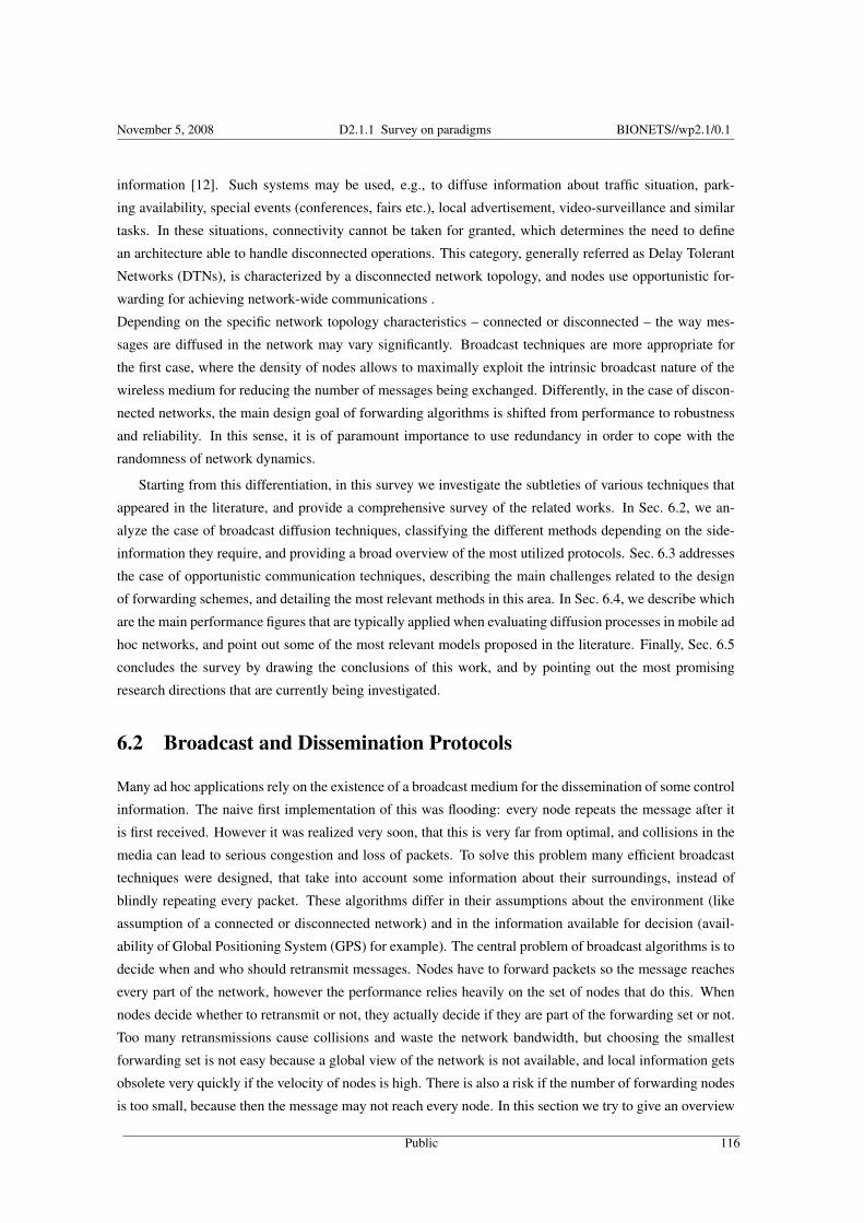
November 5, 2008 D2.1.1 Survey on paradigms BIONETS//wp2.1/0.1
information [12]. Such systems may be used, e.g., to diffuse information about traffic situation, park-
ing availability, special events (conferences, fairs etc.), local advertisement, video-surveillance and similar
tasks. In these situations, connectivity cannot be taken for granted, which determines the need to define
an architecture able to handle disconnected operations. This category, generally referred as Delay Tolerant
Networks (DTNs), is characterized by a disconnected network topology, and nodes use opportunistic for-
warding for achieving network-wide communications .
Depending on the specific network topology characteristics – connected or disconnected – the way mes-
sages are diffused in the network may vary significantly. Broadcast techniques are more appropriate for
the first case, where the density of nodes allows to maximally exploit the intrinsic broadcast nature of the
wireless medium for reducing the number of messages being exchanged. Differently, in the case of discon-
nected networks, the main design goal of forwarding algorithms is shifted from performance to robustness
and reliability. In this sense, it is of paramount importance to use redundancy in order to cope with the
randomness of network dynamics.
Starting from this differentiation, in this survey we investigate the subtleties of various techniques that
appeared in the literature, and provide a comprehensive survey of the related works. In Sec. 6.2, we an-
alyze the case of broadcast diffusion techniques, classifying the different methods depending on the side-
information they require, and providing a broad overview of the most utilized protocols. Sec. 6.3 addresses
the case of opportunistic communication techniques, describing the main challenges related to the design
of forwarding schemes, and detailing the most relevant methods in this area. In Sec. 6.4, we describe which
are the main performance figures that are typically applied when evaluating diffusion processes in mobile ad
hoc networks, and point out some of the most relevant models proposed in the literature. Finally, Sec. 6.5
concludes the survey by drawing the conclusions of this work, and by pointing out the most promising
research directions that are currently being investigated.
6.2 Broadcast and Dissemination Protocols
Many ad hoc applications rely on the existence of a broadcast medium for the dissemination of some control
information. The naive first implementation of this was flooding: every node repeats the message after it
is first received. However it was realized very soon, that this is very far from optimal, and collisions in the
media can lead to serious congestion and loss of packets. To solve this problem many efficient broadcast
techniques were designed, that take into account some information about their surroundings, instead of
blindly repeating every packet. These algorithms differ in their assumptions about the environment (like
assumption of a connected or disconnected network) and in the information available for decision (avail-
ability of Global Positioning System (GPS) for example). The central problem of broadcast algorithms is to
decide when and who should retransmit messages. Nodes have to forward packets so the message reaches
every part of the network, however the performance relies heavily on the set of nodes that do this. When
nodes decide whether to retransmit or not, they actually decide if they are part of the forwarding set or not.
Too many retransmissions cause collisions and waste the network bandwidth, but choosing the smallest
forwarding set is not easy because a global view of the network is not available, and local information gets
obsolete very quickly if the velocity of nodes is high. There is also a risk if the number of forwarding nodes
is too small, because then the message may not reach every node. In this section we try to give an overview
Public 116

November 5, 2008 D2.1.1 Survey on paradigms BIONETS//wp2.1/0.1
of the existing algorithms and approaches by giving a categorization and showing some of the interesting
techniques. There are many possible ways to categorize dissemination protocols, one of the most used is in
[67], which we also use as a basis, and extend it where it is needed. Giving a strict, orthogonal categoriza-
tion, where an algorithm is part of exactly one class is in fact not feasible because there are many hybrid
approaches that fall into many categories, and exploit different approaches simultaneously. Instead of this,
we provide a usable, but not necessarily rigorous classification of algorithms. This way we can follow the
conventions already established in the field. We try to show what approaches are common for dissemination
protocols, and how the existing solutions relate to these approaches. In the following sections (6.2.1, 6.2.2
and 6.2.3) we give three classifications which capture three different aspects of dissemination algorithms.
These classes are overlapping, and capture different aspects of the existing algorithms. In 6.2.1 we show
what kind of information can be used to optimize broadcasting.
6.2.1 Categorization by the used information
The dissemination algorithms use different information about their environment to make their decisions.
When one has to choose from the bag of existing algorithms, one has to first investigate if the needed
information is available in the target network. Good examples for this are the dissemination methods
that use location information. Another example can be the use of some beacon mechanism, where nodes
explicitly notify others about their presence. If our network devices cannot acquire the information needed
by a broadcast method, then we could not use that algorithm. However, when such an information is
available, the efficiency of broadcasting can be greatly improved and the use of bandwidth can be reduced.
Simple heuristic based algorithms
These algorithms use very limited information about their environment. Usually they do not require pe-
riodically updated information about their neighbors, instead they watch the events of their surroundings,
like successful transmissions, collisions, or the number of duplicate packets, and try to figure out whether
the rebroadcast of data is needed or not. One of the most frequently used environment information is the
number of received duplicates of a packet, like in the Counter Based Method [53]. Because these simple
algorithms depend on heuristics, they often have some adjustable parameters, which are loosely based on
the physical world, and incorporate the intuition of the designer. Determining the optimal value for these
parameters is not easy. To solve this problem many of the algorithms in this category have an adaptive
version, which try to figure out the optimal values for the internal parameters. Most of these algorithms are
very simple, and they are usually outperformed by the more complex ones. It is also very hard to design
good heuristics, that actually work in real world scenarios, too. However, in [17] the author shows, how
simple learning algorithms — like a decision tree learning — are able to mimic the behavior of complex
ones almost perfectly while using much simpler decision rules than the original ones. This suggests, that
while good heuristics are very hard to produce ”by hand” there are very good performing heuristics, that
can be found by learning algorithms or genetic algorithms (or even by a combination of both).
Public 117

November 5, 2008 D2.1.1 Survey on paradigms BIONETS//wp2.1/0.1
Neighbor information based algorithms
These algorithms use some information about the local topology around the sender. To acquire this, these
algorithms need to use periodic HELLO messages that indicate the presence of a node. These beacon
messages may contain additional topology information on neighbors of the sender. Some of the algorithms
collect knowledge about their immediate neighbors solely, others use k-hop information (where k = 2 in
most of the cases). In this case, the algorithms know the local topology with higher precision, and so they
can coordinate the forwarding of messages much more efficiently. Often these algorithms are sensitive to
high nodes speed, because their local topology view gets outdated very quickly, so the efficiency of their
forwarding policy drops. To overcome this, broadcast algorithms may choose to send topology updates
more often, however this can lead to channel congestion.
Location based algorithms
Location based algorithms use some spatial information to make their decision. In most of the cases this
means that the device should have a Global Positioning System (GPS) to acquire this information. These
methods use HELLO messages, just like the neighbor information (section 6.2.1) algorithms do, but they
collect the location of the neighbors too. There are also algorithms that need to know only the distance to
their neighbors [39], which may be measured by signal power. In this case, the use of HELLO messages
may not be necessary. The location based algorithms can perform very well (especially when combined with
neighbor information), because of their very precise view of the local topology. However, the performance
of these algorithms is not well understood when the error of the positioning system cannot be neglected.
6.2.2 Categorization by strategy
In section 6.2.1 we showed what kind of information can be used by the different algorithms in the litera-
ture. However this information can be processed in different ways. Again, we must emphasize that these
categories are not exclusive, and some of the algorithms are put into a separate class just because they are
usually discussed together in the literature.
Stochastic
These algorithms inhibit some intrinsic random behavior that do not come from the randomness of the
environment. The benefit of this can be the elimination of coupling between the decisions of neighbors,
so the mathematical properties of these algorithms may become easier to derive (this is very similar to
randomization in statistics). This way, the selection of an appropriate parameter value can be supported by
some mathematical results, which is a clear benefit compared to the ad hoc methods sometimes used for
setting parameters. The drawback is that in some cases a random behavior may destroy some information for
the neighboring nodes, as the behavior of the algorithm is no longer deterministic. Usually the behavior is
adaptable to different situations by adjusting the probabilities of different decisions. Many of the stochastic
algorithms are heuristic based. Some of the algorithms have some Media Access Control that introduces
non-deterministic behavior. While these algorithms could be treated as stochastic algorithms, we prefer to
refer to them as deterministic.
Public 118
November 5, 2008 D2.1.1 Survey on paradigms BIONETS//wp2.1/0.1
Deterministic
These algorithms use usually some simple information about their environment (so they usually fall also in
the Simple Heuristic Based category, see section 6.2.1) and behave always the same when the environment
is the same. One of the simplest examples is the Counter Based Method already discussed in subsection
6.2.1. Among the deterministic algorithms, the ones based on graph theory have a special status, and are
usually discussed separately. These algorithms also have their own literature [46, 68, 18, 43], they use more
solid mathematical models instead of simple ad hoc heuristics, and usually rely heavily on graph theory
results. Basically two types of such algorithms exist, depending on who makes the decision about being a
forwarding node or not. Self-pruning methods let every node decide to retransmit or not, while nodes using
designation protocols explicitly choose which neighbors should be forwarding nodes.
The self-pruning algorithms collect neighborhood information from other nodes, and make a local de-
cision whether to forward the message or not [68]. Nodes can decide their forwarding status when the
neighborhood information is updated (on-update) or when the broadcast packet is first received (on-the-
fly). The usual goal of these algorithms is to approximate a minimal connected dominating set (MCDS)
[38]. A node set is a Connected Dominating Set (CDS) if every node is in the set, or is the neighbor of
a node in the set. An MCDS is the smallest of the possible Connected Dominating Sets. An approxima-
tion scheme has been adopted to distributed systems in [42, 16] primarily for the use in wireless ad hoc
networks.
Designation protocols on the other hand try to choose the forwarding nodes among themselves by
explicitly designating a node to be a forwarder. Usually a node selects a subset of nodes from his 1-hop
neighbors to be forwarding nodes for its 2-hop neighbors. The list of the designated forward nodes is usually
sent with the broadcast packet [68]. The goal for neighbor designation protocols is the same as for the self-
pruning protocols to approximate a minimal connected dominating set (MCDS). In [68] the authors give a
generalization of the idea that incorporates most of the self-pruning and neighbor designation algorithms as
special cases.
6.2.3 Categorization by media access
In every problem which have to be solved over wireless medium we have to deal with the problem of media
access. This is a big difference from wired networks, where much of the details of the network can be
abstracted away. Unfortunately wireless networks are quite "hostile” and unresponsible abstractions of the
medium can lead to poorly performing designs. Broadcast algorithms are no different, so we dedicate this
subsection to discuss some of the approaches that different algorithms use.
Some methods assume Media Access to be solved by a lower layer. These algorithms usually suppose a
MAC mechanism that does not use an RTS/CTS (Ready To Send/Clear To Send) handshake because this can
degrade the performance of the broadcasting algorithms. Most of the algorithms use instead a random jitter
to minimize collisions with other nodes. This is enough in most of the cases to avoid packet loss. However
some of the algorithms use a more elaborate random backoff algorithm. One of the most used approach
is called Random Assessment Delay (RAD) which was first introduced in [53]. Algorithms using a RAD
mechanism do not retransmit messages immediately, but instead they wait for a random time. During this
time they are able to collect more information about their environment. After the RAD expires they can
Public 119
November 5, 2008 D2.1.1 Survey on paradigms BIONETS//wp2.1/0.1
cancel or proceed with the retransmission, according to the events that happened during the RAD. Some
algorithms vary the length of the possible RAD period according to local congestion levels. In other cases
RAD is used as a prioritization method to make some of the nodes more likely to broadcast first (usually the
ones with the most neighbors). We should note that the use of RAD creates non-deterministic behavior, but
we prefer to discuss this under Media Access, and not to treat the resulting algorithms as stochastic. There
are also broadcast algorithms, that adjust the signal levels of the network interfaces in a coordinated way, to
improve the efficiency of broadcasts. Of course these approaches need specialized equipment at the nodes.
6.2.4 Survey of existing algorithms
There are many published comparisons of information dissemination methods [40, 18, 67, 2, 33], which
provide us a quite detailed picture about the existing broadcast approaches. In this section we will try to
give a quick overview of the most important methods.
The Counter Based Method, originally introduced in [53], is one of the first controlled broadcast meth-
ods, and it is a deterministic, heuristic based algorithm. It is based on a simple observation, that if a duplicate
of a packet is received, then the probability of reaching any new node is low. To exploit this idea, the nodes
do not immediately transmit on the receipt of a packet, but instead they wait for a random time, which is
called Random Assessment Delay (RAD). If a duplicate is received during the RAD a counter is increased.
If the counter reaches a threshold before the RAD expires, the node cancels the transmission. The original
method has different adaptive versions [2], which try to adapt the length of RAD and the threshold of the
duplicate counter to the current network conditions.
Another very simple broadcast method is the Gossiping algorithm which was also introduced in [53]. It
is a very simple one: every node broadcasts the heard message with a predefined probability. The optimal
probability can be calculated off-line, or can be learned adaptively. Some of these adaptive versions are
covered in [15]. While the Counter Based method is a fine example of a simple heuristic based deterministic
algorithm, the Gossiping is an example for the simple heuristic based stochastic methods. While it is very
easy to implement, it is usually outperformed by other more sophisticated algorithms. Another problem
can be, that while the optimal retransmission probability can be calculated off line, it heavily relies on
the parameters of the environment. To overcome this limitation there are adaptive versions of the basic
methods, like Hypergossiping.
Hypergossiping [37] is one of the most recent algorithms discussed in this document. It is specifically
designed for partitioned networks, where nodes are mobile, and partitions join and split from time to time. It
is an advanced version of the Gossip algorithm, extended by neighbor information and partition join detec-
tion. The algorithm uses a simple adaptive gossiping strategy for in-partition forwarding, but rebroadcasts
some of the packets if it detects a join with another partition. The join detection is based on the simple
heuristic, that the nodes in the same partition received the same messages recently. Every node maintains
a list, called LBR (Last Broadcasts Received), of the recently broadcast messages. They send HELLO
messages periodically, to indicate their presence. When a new node is detected, one of the nodes includes
its LBR in the next HELLO message. When the other node receives this LBR, it compares with its own
LBR. If the overlap between the LBR of two nodes is smaller than a threshold, then the node is considered
coming from another partition, so a new message is sent, called BR (Broadcasts Received), which contains
Public 120
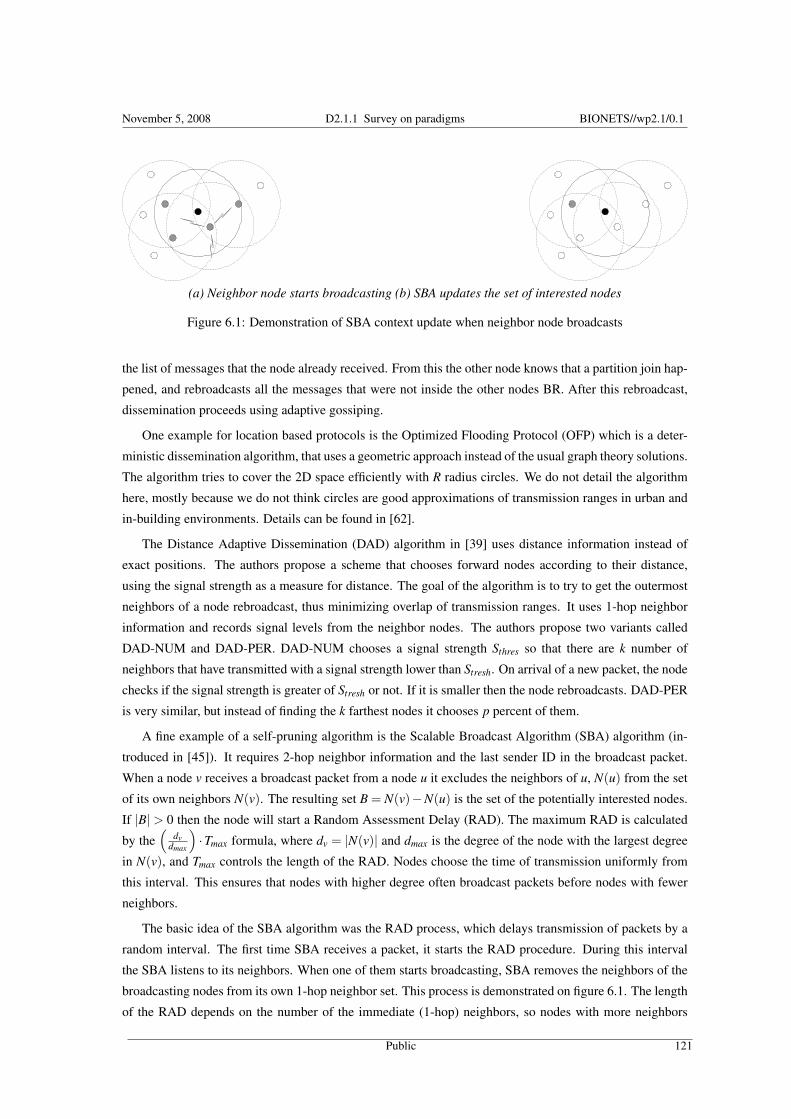
November 5, 2008 D2.1.1 Survey on paradigms BIONETS//wp2.1/0.1
(a) Neighbor node starts broadcasting (b) SBA updates the set of interested nodes
Figure 6.1: Demonstration of SBA context update when neighbor node broadcasts
the list of messages that the node already received. From this the other node knows that a partition join hap-
pened, and rebroadcasts all the messages that were not inside the other nodes BR. After this rebroadcast,
dissemination proceeds using adaptive gossiping.
One example for location based protocols is the Optimized Flooding Protocol (OFP) which is a deter-
ministic dissemination algorithm, that uses a geometric approach instead of the usual graph theory solutions.
The algorithm tries to cover the 2D space efficiently with R radius circles. We do not detail the algorithm
here, mostly because we do not think circles are good approximations of transmission ranges in urban and
in-building environments. Details can be found in [62].
The Distance Adaptive Dissemination (DAD) algorithm in [39] uses distance information instead of
exact positions. The authors propose a scheme that chooses forward nodes according to their distance,
using the signal strength as a measure for distance. The goal of the algorithm is to try to get the outermost
neighbors of a node rebroadcast, thus minimizing overlap of transmission ranges. It uses 1-hop neighbor
information and records signal levels from the neighbor nodes. The authors propose two variants called
DAD-NUM and DAD-PER. DAD-NUM chooses a signal strength Sthres so that there are k number of
neighbors that have transmitted with a signal strength lower than Stresh. On arrival of a new packet, the node
checks if the signal strength is greater of Stresh or not. If it is smaller then the node rebroadcasts. DAD-PER
is very similar, but instead of finding the k farthest nodes it chooses p percent of them.
A fine example of a self-pruning algorithm is the Scalable Broadcast Algorithm (SBA) algorithm (in-
troduced in [45]). It requires 2-hop neighbor information and the last sender ID in the broadcast packet.
When a node v receives a broadcast packet from a node u it excludes the neighbors of u, N(u) from the set
of its own neighbors N(v). The resulting set B = N(v)−N(u) is the set of the potentially interested nodes.
If |B| > 0 then the node will start a Random Assessment Delay (RAD). The maximum RAD is calculated
by the(
dvdmax
)·Tmax formula, where dv = |N(v)| and dmax is the degree of the node with the largest degree
in N(v), and Tmax controls the length of the RAD. Nodes choose the time of transmission uniformly from
this interval. This ensures that nodes with higher degree often broadcast packets before nodes with fewer
neighbors.
The basic idea of the SBA algorithm was the RAD process, which delays transmission of packets by a
random interval. The first time SBA receives a packet, it starts the RAD procedure. During this interval
the SBA listens to its neighbors. When one of them starts broadcasting, SBA removes the neighbors of the
broadcasting nodes from its own 1-hop neighbor set. This process is demonstrated on figure 6.1. The length
of the RAD depends on the number of the immediate (1-hop) neighbors, so nodes with more neighbors
Public 121
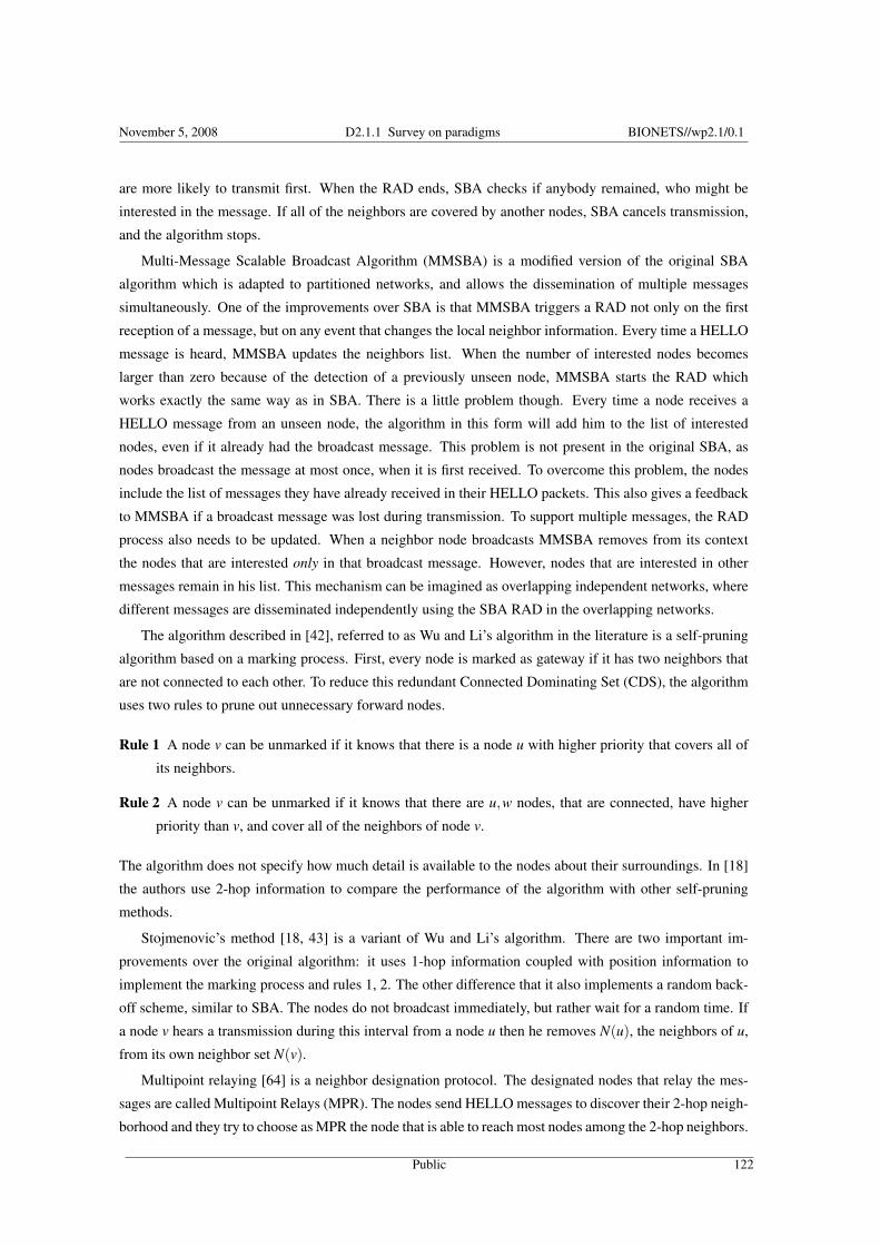
November 5, 2008 D2.1.1 Survey on paradigms BIONETS//wp2.1/0.1
are more likely to transmit first. When the RAD ends, SBA checks if anybody remained, who might be
interested in the message. If all of the neighbors are covered by another nodes, SBA cancels transmission,
and the algorithm stops.
Multi-Message Scalable Broadcast Algorithm (MMSBA) is a modified version of the original SBA
algorithm which is adapted to partitioned networks, and allows the dissemination of multiple messages
simultaneously. One of the improvements over SBA is that MMSBA triggers a RAD not only on the first
reception of a message, but on any event that changes the local neighbor information. Every time a HELLO
message is heard, MMSBA updates the neighbors list. When the number of interested nodes becomes
larger than zero because of the detection of a previously unseen node, MMSBA starts the RAD which
works exactly the same way as in SBA. There is a little problem though. Every time a node receives a
HELLO message from an unseen node, the algorithm in this form will add him to the list of interested
nodes, even if it already had the broadcast message. This problem is not present in the original SBA, as
nodes broadcast the message at most once, when it is first received. To overcome this problem, the nodes
include the list of messages they have already received in their HELLO packets. This also gives a feedback
to MMSBA if a broadcast message was lost during transmission. To support multiple messages, the RAD
process also needs to be updated. When a neighbor node broadcasts MMSBA removes from its context
the nodes that are interested only in that broadcast message. However, nodes that are interested in other
messages remain in his list. This mechanism can be imagined as overlapping independent networks, where
different messages are disseminated independently using the SBA RAD in the overlapping networks.
The algorithm described in [42], referred to as Wu and Li’s algorithm in the literature is a self-pruning
algorithm based on a marking process. First, every node is marked as gateway if it has two neighbors that
are not connected to each other. To reduce this redundant Connected Dominating Set (CDS), the algorithm
uses two rules to prune out unnecessary forward nodes.
Rule 1 A node v can be unmarked if it knows that there is a node u with higher priority that covers all of
its neighbors.
Rule 2 A node v can be unmarked if it knows that there are u,w nodes, that are connected, have higher
priority than v, and cover all of the neighbors of node v.
The algorithm does not specify how much detail is available to the nodes about their surroundings. In [18]
the authors use 2-hop information to compare the performance of the algorithm with other self-pruning
methods.
Stojmenovic’s method [18, 43] is a variant of Wu and Li’s algorithm. There are two important im-
provements over the original algorithm: it uses 1-hop information coupled with position information to
implement the marking process and rules 1, 2. The other difference that it also implements a random back-
off scheme, similar to SBA. The nodes do not broadcast immediately, but rather wait for a random time. If
a node v hears a transmission during this interval from a node u then he removes N(u), the neighbors of u,
from its own neighbor set N(v).
Multipoint relaying [64] is a neighbor designation protocol. The designated nodes that relay the mes-
sages are called Multipoint Relays (MPR). The nodes send HELLO messages to discover their 2-hop neigh-
borhood and they try to choose as MPR the node that is able to reach most nodes among the 2-hop neighbors.
Public 122
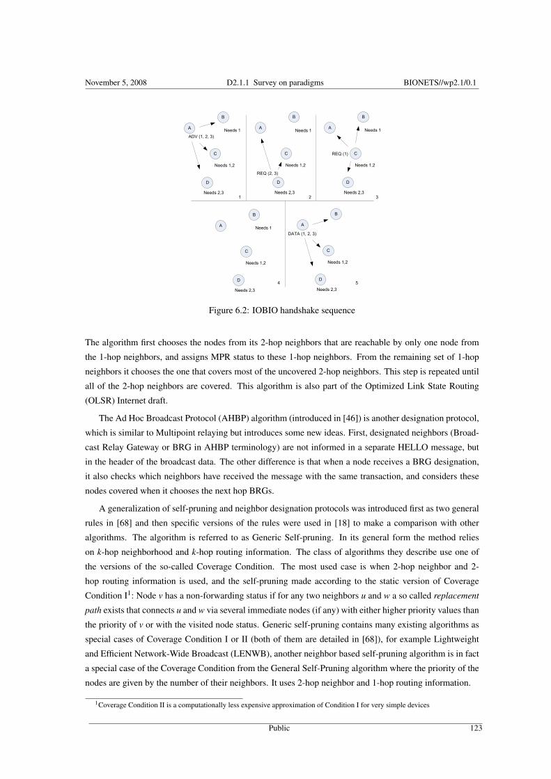
November 5, 2008 D2.1.1 Survey on paradigms BIONETS//wp2.1/0.1
Figure 6.2: IOBIO handshake sequence
The algorithm first chooses the nodes from its 2-hop neighbors that are reachable by only one node from
the 1-hop neighbors, and assigns MPR status to these 1-hop neighbors. From the remaining set of 1-hop
neighbors it chooses the one that covers most of the uncovered 2-hop neighbors. This step is repeated until
all of the 2-hop neighbors are covered. This algorithm is also part of the Optimized Link State Routing
(OLSR) Internet draft.
The Ad Hoc Broadcast Protocol (AHBP) algorithm (introduced in [46]) is another designation protocol,
which is similar to Multipoint relaying but introduces some new ideas. First, designated neighbors (Broad-
cast Relay Gateway or BRG in AHBP terminology) are not informed in a separate HELLO message, but
in the header of the broadcast data. The other difference is that when a node receives a BRG designation,
it also checks which neighbors have received the message with the same transaction, and considers these
nodes covered when it chooses the next hop BRGs.
A generalization of self-pruning and neighbor designation protocols was introduced first as two general
rules in [68] and then specific versions of the rules were used in [18] to make a comparison with other
algorithms. The algorithm is referred to as Generic Self-pruning. In its general form the method relies
on k-hop neighborhood and k-hop routing information. The class of algorithms they describe use one of
the versions of the so-called Coverage Condition. The most used case is when 2-hop neighbor and 2-
hop routing information is used, and the self-pruning made according to the static version of Coverage
Condition I1: Node v has a non-forwarding status if for any two neighbors u and w a so called replacement
path exists that connects u and w via several immediate nodes (if any) with either higher priority values than
the priority of v or with the visited node status. Generic self-pruning contains many existing algorithms as
special cases of Coverage Condition I or II (both of them are detailed in [68]), for example Lightweight
and Efficient Network-Wide Broadcast (LENWB), another neighbor based self-pruning algorithm is in fact
a special case of the Coverage Condition from the General Self-Pruning algorithm where the priority of the
nodes are given by the number of their neighbors. It uses 2-hop neighbor and 1-hop routing information.
1Coverage Condition II is a computationally less expensive approximation of Condition I for very simple devices
Public 123

November 5, 2008 D2.1.1 Survey on paradigms BIONETS//wp2.1/0.1
A quite different approach from the algorithms discussed so far is the IOBIO algorithm[63]. It is a
variation of the SPIN [27] dissemination protocol. It uses a simple 3-stage handshake to discover neighbors
that are interested in one of the carried messages. The goal of the protocol is to reduce the unnecessary load
of neighboring nodes by duplicate or unneeded data ("spamming”). There are three IOBIO message types
that are used by the protocol. The ADV (Advertisement) messages are sent periodically, and they contain
the list of messages that the sending node has. Neighbor nodes indicate their interest in the advertised
messages by sending a REQ (Request) packet. In response to the REQ, the originator node sends the
required DATA packets. The transmission of a REQ after an ADV is not done immediately, but after a
random delay. During this delay, the nodes listen to each other, and they only request packets that were not
requested before. This process is demonstrated on Figure 6.2. Node A sends an advertisement indicating
that it has the messages 1, 2 and 3. After receiving this ADV, nodes B, C, D start a random delay. At step
2 node D sends a REQ packet, indicating, that he needs messages 2 and 3. At step 3, node C sends a REQ
packet. However, he heard the REQ packet of D, so he knows, that message 2 is already requested, and only
puts the ID of message 1 in the REQ packet. At step 4, the random delay of B is over, however, message 1
is already requested, so no REQ is sent. At step 5 the wait interval of node A is over, and it broadcasts all
requested messages.
6.2.5 General comparison and discussion
Table 6.1 summarizes the algorithms discussed in the previous sections. The main aspect of classification
of dissemination protocols in dense mobile ad hoc network is the strategy used to effectively propagate
information in the system. Simple heuristic based and stochastic methods are usually outperformed by the
more sophisticated approaches like neighbor or location based strategies. An important constraint can be
the availability of special hardware e.g. GPS devices for location based methods meanwhile most of the
neighbor based schemes do not need any additional support. In dense scenarios neighbor based protocols
can dramatically decrease redundancy of dissemination at the cost of increasing the overall amount of
control messages. Another drawback could be the sensitivity to fast topology changes caused by high
velocity nodes. A different aspect of comparison could be where is the forwarding status decided: at the
node itself, or by the previous node. An exception to this is MIOBIO which uses a handshake mechanism
which means that a negotiation process is carried out among the interested and forwarding nodes. Many
times it is useful to be able to disseminate messages of different services in parallel, only Hypergossip,
MMSBA and MIOBIO provides this feature.
6.3 Routing Approaches for Intermittently Connected Networks
Intermittently connected networks are a new class of wireless networks that started to emerge recently and to
gain extensive efforts from the networking research community. In the literature, these networks are found
under different terminology such as sparse or extreme wireless networks, or under another commonly used
term disruption/delay tolerant networks (DTNs) [1],[20]. These schemes arise in areas where the network
spans over large distances with a low and heterogeneous node density and where the presence of a fixed
infrastructure has no great impact on the lack of connectivity of the network. Examples of such networking
scenarios include disaster healing and military networks, vehicular networks [54], deep space networks
Public 124
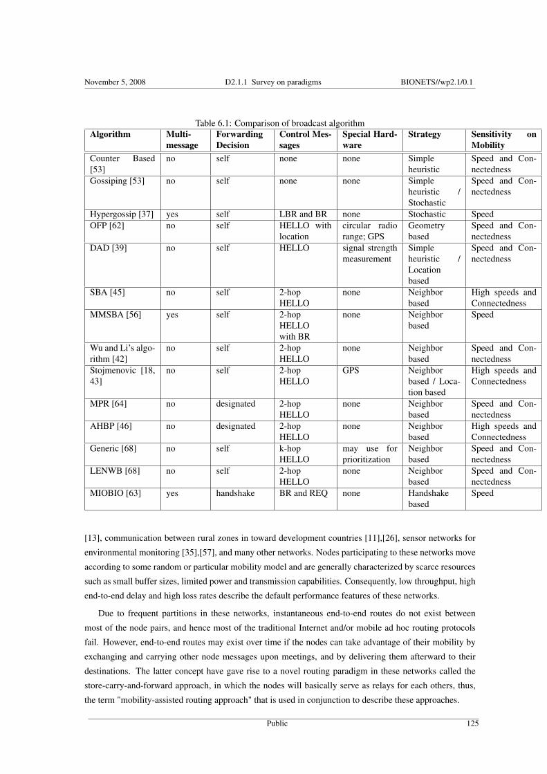
November 5, 2008 D2.1.1 Survey on paradigms BIONETS//wp2.1/0.1
Table 6.1: Comparison of broadcast algorithmAlgorithm Multi-
messageForwardingDecision
Control Mes-sages
Special Hard-ware
Strategy Sensitivity onMobility
Counter Based[53]
no self none none Simpleheuristic
Speed and Con-nectedness
Gossiping [53] no self none none Simpleheuristic /Stochastic
Speed and Con-nectedness
Hypergossip [37] yes self LBR and BR none Stochastic SpeedOFP [62] no self HELLO with
locationcircular radiorange; GPS
Geometrybased
Speed and Con-nectedness
DAD [39] no self HELLO signal strengthmeasurement
Simpleheuristic /Locationbased
Speed and Con-nectedness
SBA [45] no self 2-hopHELLO
none Neighborbased
High speeds andConnectedness
MMSBA [56] yes self 2-hopHELLOwith BR
none Neighborbased
Speed
Wu and Li’s algo-rithm [42]
no self 2-hopHELLO
none Neighborbased
Speed and Con-nectedness
Stojmenovic [18,43]
no self 2-hopHELLO
GPS Neighborbased / Loca-tion based
High speeds andConnectedness
MPR [64] no designated 2-hopHELLO
none Neighborbased
Speed and Con-nectedness
AHBP [46] no designated 2-hopHELLO
none Neighborbased
High speeds andConnectedness
Generic [68] no self k-hopHELLO
may use forprioritization
Neighborbased
Speed and Con-nectedness
LENWB [68] no self 2-hopHELLO
none Neighborbased
Speed and Con-nectedness
MIOBIO [63] yes handshake BR and REQ none Handshakebased
Speed
[13], communication between rural zones in toward development countries [11],[26], sensor networks for
environmental monitoring [35],[57], and many other networks. Nodes participating to these networks move
according to some random or particular mobility model and are generally characterized by scarce resources
such as small buffer sizes, limited power and transmission capabilities. Consequently, low throughput, high
end-to-end delay and high loss rates describe the default performance features of these networks.
Due to frequent partitions in these networks, instantaneous end-to-end routes do not exist between
most of the node pairs, and hence most of the traditional Internet and/or mobile ad hoc routing protocols
fail. However, end-to-end routes may exist over time if the nodes can take advantage of their mobility by
exchanging and carrying other node messages upon meetings, and by delivering them afterward to their
destinations. The latter concept have gave rise to a novel routing paradigm in these networks called the
store-carry-and-forward approach, in which the nodes will basically serve as relays for each others, thus,
the term "mobility-assisted routing approach" that is used in conjunction to describe these approaches.
Public 125
November 5, 2008 D2.1.1 Survey on paradigms BIONETS//wp2.1/0.1
This part will survey and classify various research works that have considered routing schemes for inter-
mittently connected networks. Actually, there are different ways to categorize these approaches. Hereafter,
we propose a classification that is based on the degree of knowledge that the nodes have about their future
contact opportunities 2 with other nodes. Specifically, depending on whether these contact opportunities
are scheduled, controlled, predicted or opportunistic, these approaches can be grouped into one of the four
following families.
6.3.1 Scheduled-contact based routing
This section surveys the routing approaches that attempt to improve the performance of a sparse network
when its dynamics are known in advance such as for instance Low-earth Orbiting satellites (LEO) based
networks. In a given network scenario, the most important metrics of interest are the following. The contact
times between nodes (their starting times and durations), queue lengths of the nodes, and the network traffic
load. The complete knowledge of these three metrics by the routing protocol allows to select optimal routes
between the nodes. Despite that the implementation of the complete knowledge in a distributed environment
is a very hard task, its evaluation is important as it constitutes the best case scenario compared with other
case where only a partial knowledge is available to the routing protocol. On the other side, the approaches
that use zero knowledge constitute the worst case scenario.
Jain et al. in [31] use the delay of a link as a cost function, and define the cost of a route to be the sum
of its link costs. The authors propose four different techniques that utilize different degrees of knowledge.
The first proposal is the Minimum Expected Delay (MED) where only the expectation of the link delay
(excluding queueing delay) is known by the routing protocols. The second is the Earliest Delivery (ED)
where the instantaneous link delay is available. The third is the Earliest Delivery with Local Queueing
(EDLQ) where in addition to the use of the instantaneous delay, the delay at the local queue node is known.
The last is the Earliest Delivery with All Queues (EDAQ) where in addition to the link delays, all the delays
of the nodes queues are known. All these approaches were evaluated using simulation and compared to
the zero knowledge and the complete knowledge cases. Their conclusion is that in networks with plentiful
communication opportunities, the need for smart algorithms that require more knowledge is minimal. In
situation where resources are limited smarter algorithms (EDLQ and EDAQ) may provide a significant
benefits.
6.3.2 Controlled-contact based routingapproaches
In this section, we discuss some routing approaches in DTNs which control the mobility of some dedicated
additional mobile nodes in order to improve the network performance by increasing the contact opportuni-
ties between participating nodes. The additional mobile nodes can either have fixed predetermined paths
conceived in a way to permit them to meet a large number of nodes, or their paths can be adjusted dynami-
cally to meet traffic flows between the nodes. Their main task is to relay packets between the participating
nodes by providing a store-carry-forward service. Indeed, by controlling the mobility of the additional
nodes, a DTN network administrator would be able to limit the delivery delay and to provide bounds on
2Two nodes are in contact if they are within transmission range of one another.
Public 126

November 5, 2008 D2.1.1 Survey on paradigms BIONETS//wp2.1/0.1
some other performance metrics of the network. In the literature, several research works have discussed
the integration of some special mobile nodes and the design of travel paths of these nodes to meet certain
optimization criteria.
Jain et al. in [32] have introduced and modeled an architecture of a sparse network constituted by
fixed sensors and extended by mobile nodes called MULEs (Mobile Ubiquitous LAN Extensions). MULEs
move in the network area according to a random mobility model. Their task is to collect data from sensors,
buffer it and drop it off later to a set of fixed base stations representing data sinks. The main objective
of the architecture is to enhance power saving by allowing sensor nodes to exploit the random mobility
of MULEs by transmitting their data to these mobile nodes over short range radio links when they pass
nearby. To characterize data success ratio and queueing delay at the sensor buffer, the authors introduce
a simple stochastic model based on renewal theory and bulk queueing theory. Through simulations, they
have also investigated other performance metrics when the system parameters, the number of access points
and the number of MULEs scale. Their basic observation confirms that an increase in the MULE density
will improve system performance and leverage resource consumption.
Another controlled-contact routing work that is based on a proactive approach has been introduced in
[70]-[71] by Zhao et al.. The approach is termed proactive in the sense that the trajectories of the special
mobile nodes, termed as message ferries (MF), are already determined and fixed. Under the assumption of
mobility of network nodes, the authors consider two schemes of messages ferries, depending on whether
nodes or ferries initiate the proactive movement. In the Node-Initiated Message Ferrying (NIMF) scheme,
ferries move around the area according to known routes, collect messages from the nodes and deliver the
messages later to their corresponding destinations. Aware of the ferries routes, the mobile nodes can adapt
their trajectories to meet the ferries in order to transmit and receive messages. In the Ferry-Initiated Message
Ferrying (FIMF), the ferries will move upon service requests to meet the nodes. Specifically, when a node
has packets to send or to receive, it generates a service request and transmits it to a chosen ferry using a long
range radio. When the ferry receives the request, it adapts its trajectory to meet with the node for packet
exchanging using short range radio.
In their former work [70], the focus was on the design of ferry routes to meet certain constraints on
throughput requirement and delivery delay in networks with stationary nodes using a single ferry. By for-
mulating the problem as two optimization sub-problems, they developed algorithms to design the ferry
route. In a recent work [72], they considered the case of multiple ferries with the possibility of interaction
between the ferries. The addition of multiple ferries has the advantages of improving the system perfor-
mance and robustness to ferry failure at the cost of increasing the complexity of the problem. Based on
several assumptions regarding whether the ferries follow the same or different routes and whether they in-
teract with each others, they investigated four different route design algorithms that attempt to meet the
traffic demand and minimize the delivery delay. Simulation results showed that when the traffic load is low,
the impact of increasing the number of ferries on the delivery delay is minor. However, for high traffic load
scenarios, the impact is significant.
In [14], the authors propose an algorithm called MV routing which, on one side, exploits the movement
patterns of participating nodes, that is the meeting and visit behaviors, and on the other side, attempts to
control the motions of some additional external nodes. Their aim is to improve network efficiency in terms
of bandwidth and latency of message delivery. The algorithm is seen as being constituted by two separate
Public 127
November 5, 2008 D2.1.1 Survey on paradigms BIONETS//wp2.1/0.1
mechanisms. Building on their previous work in [19], the first mechanism is a slightly modified variant
of the Drop-Least-Encountered technique that is used as a routing strategy instead of a buffer management
technique as it has been used in [19]. The second mechanism of the algorithm consists in adapting dynam-
ically the movement paths of some additional nodes to meet the traffic demands in the network while op-
timizing some performance criterion. Travel path adjustment is carried out through multi-objective control
algorithms with the objective of optimizing simultaneously several metrics related to bandwidth and delay.
Simulation results demonstrate that exploiting node mobility patterns in conjunction with multi-objective
control for autonomous nodes have the most significant performance improvements.
6.3.3 Predicted-contact based routingapproaches
Predicted routing techniques attempt to take advantage of certain knowledge concerning the mobility pat-
terns or some repeating behavioral patterns. Based on an estimation of that knowledge, a node will decide
on whether to forward the packet or to keep it and wait for a better chance. Basically, each node is as-
signed a set of metrics representing its likelihood to deliver packets to a given destination node. When a
node holding a packet meets another node with a better metric to the destination, it passes the packet to
it, hence increasing the packet likelihood of being delivered to its corresponding destination. According to
the nature of knowledge, we propose to reclassify the algorithms falling under this category as based on
mobility-pattern or based on history.
Mobility-pattern based approaches
Approaches falling under this section attempt to take advantage of common behaviors of node mobility
patterns in the network in order to derive decisions on packet forwarding. In fact, by letting the nodes learn
the mobility pattern characteristics in the network, efficient packet forwarding decisions can be taken. Two
main issues are related to these approaches. The first issue concerns the definition and the characterization
of the node mobility pattern where several ways can exist to characterize and acquire such a pattern. For
instance, the appearance of stable node clusters in the network, or the acquisition of statistical information
related to meeting times or to the visit frequencies of nodes to a given set of locations are examples of
mobility patterns that can be exploited by the nodes. The second issue is related to the way through which
a node can learn and acquire its own pattern as well as those of other nodes. In particular, the presence of
some external signals to the nodes such as GPS coordinates or some fixed beacons help greatly the nodes to
acquire easily the mobility patterns in the network. Alternatively, nodes can also learn their own mobility
patterns without any external signal by relying only on previous observations and measurements, or by
exchanging pattern information with other nodes. Several routing works in DTNs that use mobility patterns
to derive forwarding decisions have appeared in the literature.
In [55], the authors develop a routing algorithm that exploits the presence of concentration points (CPs)
of high node density in the network to optimize forwarding decisions. The appearance of CPs is seen as
the result of a general mobility model where nodes will have a high concentration inside these CPs with
random movements over time between these islands of connectivity. The basic idea of their algorithm is to
make use of the neighbor set evolution of each node without using any external signals. Specifically, nodes
Public 128

November 5, 2008 D2.1.1 Survey on paradigms BIONETS//wp2.1/0.1
that belong to a given concentration point will collaborate between them to assign a label to their CP. Nodes
will learn the labels of other nodes when they move in the network between the different CPs. Using the
knowledge of the CP graph, and the positions of the source and destination nodes in the graph, the message
is forwarded from the source to its destination through a sequence of CPs using the shortest path between
the respective CPs. Even though the algorithm performs well, the need to manage and update the labels
introduces some complexity in the algorithm mechanism.
In another work [41], the authors introduce a virtual-location routing scheme which makes use of the
frequency of visit of nodes to a discrete set of locations in the network area in order to decide on packet
forwarding. Specifically, they define a virtual Euclidean space, termed as MobySpace, where the dimension
degree and the type of the coordinate space depend on the mobility pattern of the nodes. For instance, for
a network with L possible node locations, the MobySpace is an n-dimensional space where n = |L|. Each
node is represented in that space by a virtual coordinate termed as MobyPoint. A source node X with a
message to send at time t will forward its message to a node Y among the set of its neighbors WX (t) for
which the Euclidean distance to the destination is the smallest. Observe that the MobyPoint of a node is not
related to its physical GPS coordinate. The acquisition of the visit frequencies of the nodes to the location
set is obtained by computing the respective fraction of time of being in a given location.
Another subclass of mobility-pattern based approach consists in exploiting the underlying structure of
social aspects of the network, whether in terms of contact patterns as well as set of interests, in order to de-
rive decisions on packet forwarding. Actually, accounting for the social interactions and the social structure
of the network to which the mobile users belong was proved to significantly influence the routing perfor-
mance of the network. Various groups have recently started investigating the impact of social aspects on
forwarding protocol design and routing performance.
In [28], the community structure behind the social interactions has been studied in order to improve the
forwarding algorithms in the network. The authors showed that there exists a limited set of nodes, called
hubs, which play a central role in the diffusion of information. Being aware of the community structure, the
authors showed that an extremely efficient trade-off between resources and performance can be achieved.
In [48], the impact of different social-based forwarding schemes were evaluated on real world mobility pat-
terns obtained from Bluetooth proximity measures. The authors showed that incorporating a friend/stranger
classification in the forwarding policies can be beneficial in different application scenarios.
History based approaches
History based approaches are developed mainly for heterogeneous mobility movements. They rely on the
observation that the future node movements can be effectively predicted based on repeating behavioral
patterns. For instance, if a node had visited a location at some point in time, it would probably visit that
location in another future time. Actually, if at any point in time a node can move randomly over the network
area, an estimate based on previous contacts is of no help to decide on packet forwarding. However, if
the mobility process has some locality, then last encounter times with other nodes can be associated with
some weights that can be ranked based on their likelihood to deliver the messages to the corresponding
destinations. The following works illustrate the working mechanisms of some of these approaches.
One of the pioneer work that considered history-based routing in sparse mobile networks is the work
of Davis et al. in [19]. The objective of their work is to study the impact of different buffer management
Public 129

November 5, 2008 D2.1.1 Survey on paradigms BIONETS//wp2.1/0.1
techniques on an extended variant of the epidemic protocol [61] on nodes with limited buffer size. Even
though their work is not related to routing, the way by which the packets are sorted upon a contact influ-
ences implicitly the performance of the routing protocol. More precisely, when two nodes meet, they will
first transfer the packets destined to each other, then they will exchange the lists of their remaining stored
packets. The combined list of remaining packets is next sorted according to the used buffer management
strategy, and each node will request the packets it does not have among the top K sorted packets. The au-
thors have explored four different buffer management techniques, among them the Drop-Least-Encountered
(DLE) technique which makes use of previous contacts with other nodes to decide on packet ranking. Ba-
sically, nodes using the DLE technique keep a vector indexed by addresses of other nodes where each entry
estimates the likelihood of meeting the corresponding node. At each time step, a given node A updates its
likelihood meeting values for every other node C with respect to the co-located node B according to the
temporal difference rule (see [60]). If node A meets B, it is likely that A meets B again in the future, and
hence A is a good candidate for passing the packets to B. Thus, node A should increase its likelihood for
node B. If B has a high encounter for node C, then A should increases its likelihood of meeting C by a factor
proportional to the likelihood of meeting between B and C. Last, if at a given time step, node A did not meet
any other node, the different likelihood values decrease in a constant rate.
In [35], the authors propose a wireless peer-to-peer networking architecture, called ZebraNet system,
which is designed to support wildlife tracking for biology research. The network is basically a mobile sensor
network, where animals equipped with tracking collars act as mobile nodes which cooperate between them
in a peer-to-peer fashion to deliver collected data back to researchers. Researcher base stations, mounted
on cars, are moving around sporadically to collect logged data. The design goal is to use the least energy,
storage and other resources necessary to maintain a reliable system with a very high data delivery success
rate. To attain these objectives, they propose the use of a history-based protocol to handle packet transfer
between neighbor peer nodes. More precisely, each node will be assigned a hierarchical level based on
its past successes of transferring data to the base station. The higher the level of the node, the higher the
probability that this node is within range of base station or within range of some other nodes near the base
station. Therefore, it has a high likelihood of relaying the data back to the base station either directly or
indirectly through minimal number of other nodes. The mechanism works as follows: each time a node
scans for peer neighbors, it requests the hierarchy level of all of its neighbors. Collected data is then sent to
the neighbor with the highest hierarchy level. Whenever a node comes within range of the base station, its
hierarchy level is increased while it is decreased over time at a given rate when it is out-of-range.
Jones et al. in [34] propose a variant of the MED approach of [31] called Minimum Estimated Expected
Delay (MEED). Alternatively to the MED approach where the expected delay of a link is computed using
the future contact schedule, MEED uses an estimation of the observed contact history. The estimator
implements a sliding history window with an adjustable size. To minimize the overhead induced by the
frequent updates of the estimated link delay, the authors propose to filter update samples having small
difference with the actual information in the network. Through simulations, MEED has shown to overcome
the performance of MED as it is more responsive to network changes, and its performance approaches that
of the epidemic protocol. However, the algorithm lacks the presence of an adjustment mechanism of its
window size.
The authors in [44] propose PROPHET (Probabilistic Routing Protocol using History of Encounters
Public 130
November 5, 2008 D2.1.1 Survey on paradigms BIONETS//wp2.1/0.1
and Transitivity), a single copy history-based routing algorithm for DTNs. Similarly to [19], each node in
PROPHET will attempt to estimate a delivery predictability vector containing an entry for each other node.
For a given node X, the entry P(X ,Y ) ∈ [0,1] will represent the probability of node X to deliver a message
to a given node, for instance node Y in this case. The entries of the predictability vectors will be used
to decide on packet forwarding. Specifically, when two nodes meet, a message is forwarded to the other
node if the delivery predictability for the destination of the message is higher at the other node. In addition
to the predictability vector, a summary vector of stored packets will be also exchanged upon contact. The
information in the summary vector is used to decide on which messages to request from the other node. The
entry update process occurs upon each contact and works as follows. Nodes that are often within mutual
ranges have a high delivery predictability for each other, and hence they will increase their corresponding
delivery predictability entries. Alternatively, nodes that rarely meet are less likely to be good forwarders of
messages to each other, and hence they will reduce their corresponding delivery predictability entries.
6.3.4 Opportunistic-contact based routingapproaches
Opportunistic based approaches are generally characterized by random contacts between participating nodes
followed by potential pair-wise exchanges of data. Given that connectivity, and consequently, data ex-
changes are subject to the characteristics of the mobility model which are in general unpredicted, these
approaches rely on multi-copy schemes to speed up data dissemination within the network. In the follow-
ing, we subdivide these approaches into epidemic-based approaches and coding based approaches.
Epidemic based approaches
Epidemic based approaches imitate the spread of contagious disease in a biological environment. Simi-
larly to the way an infected individual passes on a virus to those who come into contact, each node in an
epidemic-based system will spread copies of packets it has received to other susceptible nodes. The num-
ber of copies that an infected node is allowed to make, termed as the fan-out of the dissemination, and the
maximum number of hops that a packet is allowed to travel between the source and the destination nodes,
represented by a hop count field in the packet, define the epidemic variant of the algorithm. These two
parameters can be tuned to trade delay for resource consumption. Clearly, by allowing the packet to spread
throughout the mobile nodes, the delay until one of the copies reaches the destination can be significantly
reduced. However, this comes at the cost of introducing a large overhead in terms of bandwidth, buffer
space and energy consumption. Several variants of epidemic-based approaches have been proposed and
their performance in terms of delay and resource consumption have been evaluated.
One of the pioneer work in this domain is the epidemic routing protocol of Vahdat and Becker [61]. The
protocol is basically a flooding mechanism accommodated for mobile wireless networks. It relies on pair-
wise exchanges of messages between nodes as they get in contact with each other to eventually deliver the
messages to their destinations. Each node manages a buffer containing messages that have been generated
at the current node as well as messages that has been generated by other nodes and relayed to this node. An
index of the stored messages called a summary vector is kept by each node. When two nodes meet, they
will exchange their summary vectors. After this exchange, each node can determine then if the other node
Public 131
November 5, 2008 D2.1.1 Survey on paradigms BIONETS//wp2.1/0.1
has some messages that was previously unseen by it. In this case, it will request the missing messages from
the other node. To limit the resource utilization of the protocol, the authors propose to use a hop count field
at each message that specifies the total number of epidemic exchanges that a particular message may be
subject to. They showed that by appropriately choosing the maximum hop count, delivery rates can still be
kept high while limiting resource utilization.
In [24], Grossglauser and Tse introduce a one copy two-hop relay protocol. Basically, at any time, they
will be one copy of the packet in the network, however, the copy can make at most two hops between the
source node and the destination node. Their packet dissemination algorithm can be seen as an epidemic-
like protocol with a fan-out of one and a hop count of two. The key goal of their work is to show that the
capacity of a mobile network can scale with the number of nodes by exploiting the mobility of these nodes
through a two-hop relay protocol.
Building on [61] and [24], several research works have appeared subsequently which proposed analyti-
cal models to evaluate the performance of these protocols. In [23] Groenevelt et al. introduce a multicopy
two-hop relay protocol (MTR), a variant of the two-hop relay protocol. In MTR, the source forwards a
copy of the packet to any other relay node that it encounters. Relay nodes are only allowed to forward
the packets they carry to their destinations. By modeling the successive meeting times between any pair
of mobile nodes by Poisson processes, the authors characterize the distribution of the delivery delay and
that of the total number of copies generated until the packet delivery. This work was extended in [5] by
Al Hanbali et al. under the assumption of limited lifetime of the packets, and in [4] under the assumption
of general distribution of inter-meeting times. Zhang et al. in [69] extend the work in [23] by evaluating
several variations of the epidemic protocol and some infection-recovery schemes. Inspired by [23], the au-
thors of [29] consider a sparse mobile ad hoc network equipped by throwboxes. Throwboxes are small and
inexpensive wireless devices that act as fixed relays and that are deployed to increase contact opportunities
among the nodes. By modelling the meeting times between a mobile and a throwbox as a Poisson process,
the authors characterize the delivery delay and the total number of copies generated under the MTR and the
epidemic protocol for the cases where throwboxes are fully disconnected or mesh connected.
A biological acquisition system termed as the shared wireless infostation model (SWIM) has been
introduced in [57] as a way of routing collected measurement traces between a set of sensors attached to
whales and a set of fixed infostations acting as collecting nodes. Infostations act as base stations which
connect the users to the network. Mobile nodes represented by the tagged whales move randomly within
the area and connect to the infostations when they are within range to offload their data. When two tagged
whales meet, an epidemic exchange mechanism takes place in order to accelerate the delivery of the packets
at the cost of increasing the storage space at the nodes. Through simulations, the authors showed that
sharing the data among the whales as well as increasing the number of SWIM stations reduce significantly
the end-to-end delay. The positions of infostations as well as the mobility of whales greatly affect the
system performance.
Spyropoulos et al. introduce a new routing algorithm for sparse networks in [59], termed Spray and
Wait algorithm. The algorithm disseminates a number of copies of the packet to other nodes in the network,
and then waits until one of these copies meets the destination. It consists of two phases. In the first phase,
the source node will generate a total of L copies of the message it holds, then spreads these copies to other
nodes for delivery to the destination node. The spreading process works as follows. When an active node
Public 132

November 5, 2008 D2.1.1 Survey on paradigms BIONETS//wp2.1/0.1
holding n > 1 copies meets another node, it hands off to it F(n) copies and keeps for itself the remaining
n−F(n) copies and so forth until a copy of the message reaches the destination. F is the function that
defines the spreading process. For instance, for binary spray and wait, F(n) = n2 . In the second phase,
the wait phase, if the destination is not found among the L copy-carrying nodes, then these latter nodes
will perform direct transmissions to the destination node. Using simulations, the authors show that this
technique can achieve a trade-off between efficient packet delivery and low overhead if the parameters are
carefully designed.
Coding based approaches
The approaches in Section 6.3.4 are primarily based on packet flooding in order to improve the efficiency of
packet delivery. Unfortunately, these improvements come at the expense of introducing large overhead in
the network due to redundant packet transmissions. The approaches presented in this section alleviates the
effect of flooding through the use of smarter redundant algorithms that are based on coding theory. In the
following, we consider two main coding algorithms that appeared in the literature and which have shown
their suitability to the opportunistic contact networks, namely the erasure coding and the network coding.
In the erasure coding scheme, upon receiving a packet of size m, the source produces n data blocks of
size l < m. The coding algorithm composes these blocks in a such way to allow the destination to retrieve
the original message on receiving any subset of these blocks [49]. More precisely, the transmission of the
packet is completed when the destination receives the kth block, regardless of the identity of the k≈m/l < n
blocks it has received. The blocks are forwarded to the destination through the relay nodes according
to store-carry-and-forward approach. The performance analysis of this approach in opportunistic contact
network has shown to improve significantly the worst case delay with fixed amount of overhead [4, 65].
Further, in [30] it has been shown that erasure coding improve the probability of packet delivery in DTNs
with transmissions failures.
In the network coding scheme, instead of simply forwarding the packets, nodes may transmit packets
with linear combinations of previously received ones. For example, consider the three nodes case where
nodes A and C want to exchange packets via the intermediate node B. A (resp. C) sends a packet a (resp. c)
to B, which in turn broadcasts a xor c packet to A and C. Both A and C can recover the packet of interest,
while the number of transmissions is reduced. In [66], different aspects of the operability of network coding
with limited storage resources have been discussed and different techniques have been proposed. The main
result is that network coding benefits more from node mobility and performs well in scenarios of high
packet drop rate where simple flooding approaches fail.
6.3.5 General comparison and discussion
Table 6.2 compares the various proposals that have been addressed in Section 6.3 by summarizing the main
distinguishable features of each one. Our comparison is based on four features. The first feature defines the
degree of knowledge that the nodes have about their future contact opportunities. Future contact opportu-
nities are identified as being scheduled, controlled, predicted or opportunistic. The second feature lists the
key relevant performance metrics that each proposal attempts to optimize. For instance, these metrics range
from increasing the packet delivery ratio to reducing the end-to-end delivery delay, energy consumption
Public 133
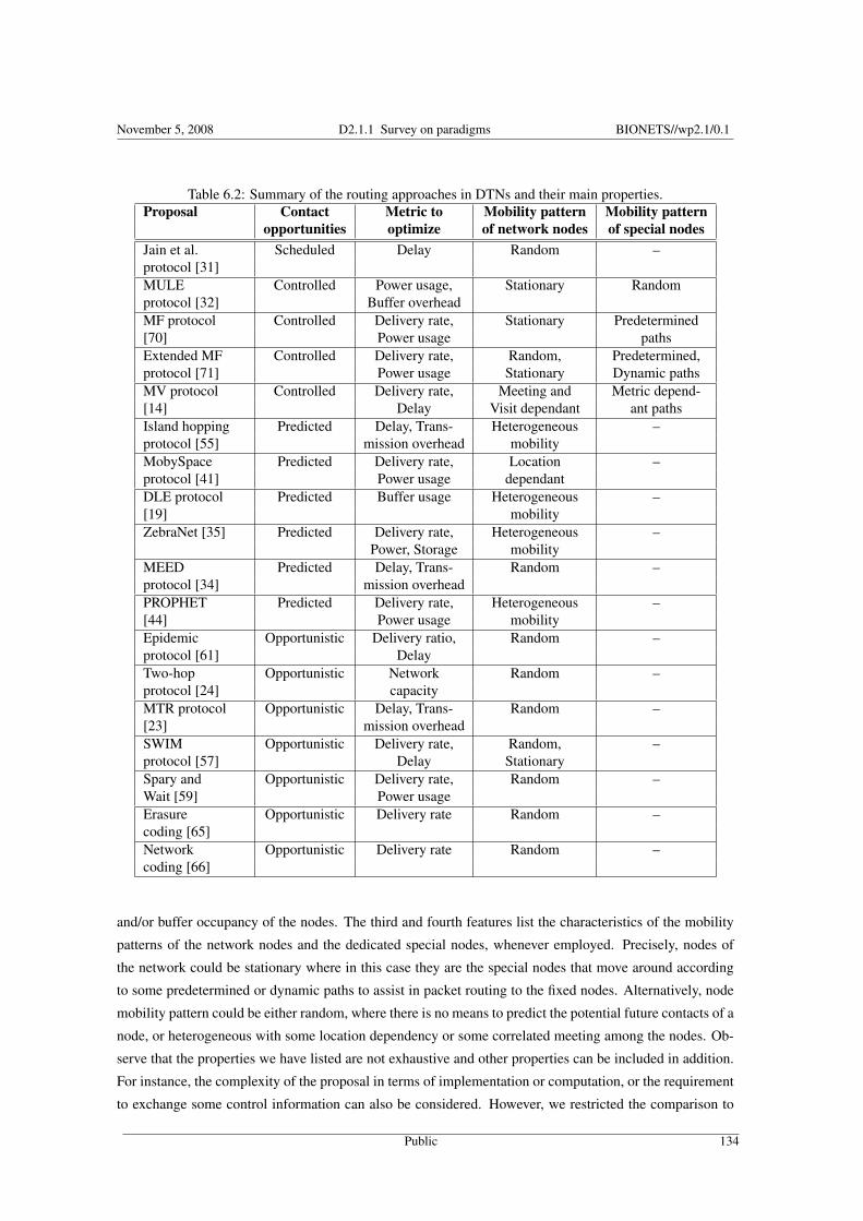
November 5, 2008 D2.1.1 Survey on paradigms BIONETS//wp2.1/0.1
Table 6.2: Summary of the routing approaches in DTNs and their main properties.Proposal Contact Metric to Mobility pattern Mobility pattern
opportunities optimize of network nodes of special nodesJain et al. Scheduled Delay Random –protocol [31]MULE Controlled Power usage, Stationary Randomprotocol [32] Buffer overheadMF protocol Controlled Delivery rate, Stationary Predetermined[70] Power usage pathsExtended MF Controlled Delivery rate, Random, Predetermined,protocol [71] Power usage Stationary Dynamic pathsMV protocol Controlled Delivery rate, Meeting and Metric depend-[14] Delay Visit dependant ant pathsIsland hopping Predicted Delay, Trans- Heterogeneous –protocol [55] mission overhead mobilityMobySpace Predicted Delivery rate, Location –protocol [41] Power usage dependantDLE protocol Predicted Buffer usage Heterogeneous –[19] mobilityZebraNet [35] Predicted Delivery rate, Heterogeneous –
Power, Storage mobilityMEED Predicted Delay, Trans- Random –protocol [34] mission overheadPROPHET Predicted Delivery rate, Heterogeneous –[44] Power usage mobilityEpidemic Opportunistic Delivery ratio, Random –protocol [61] DelayTwo-hop Opportunistic Network Random –protocol [24] capacityMTR protocol Opportunistic Delay, Trans- Random –[23] mission overheadSWIM Opportunistic Delivery rate, Random, –protocol [57] Delay StationarySpary and Opportunistic Delivery rate, Random –Wait [59] Power usageErasure Opportunistic Delivery rate Random –coding [65]Network Opportunistic Delivery rate Random –coding [66]
and/or buffer occupancy of the nodes. The third and fourth features list the characteristics of the mobility
patterns of the network nodes and the dedicated special nodes, whenever employed. Precisely, nodes of
the network could be stationary where in this case they are the special nodes that move around according
to some predetermined or dynamic paths to assist in packet routing to the fixed nodes. Alternatively, node
mobility pattern could be either random, where there is no means to predict the potential future contacts of a
node, or heterogeneous with some location dependency or some correlated meeting among the nodes. Ob-
serve that the properties we have listed are not exhaustive and other properties can be included in addition.
For instance, the complexity of the proposal in terms of implementation or computation, or the requirement
to exchange some control information can also be considered. However, we restricted the comparison to
Public 134
November 5, 2008 D2.1.1 Survey on paradigms BIONETS//wp2.1/0.1
the previous four features, which we think are the most relevant according to the classification that we made
before.
6.4 Modelling approaches
In the absence of predictable mobility and network topology, the notion of “route” for a message to follow
looses its significance, and it becomes imperative to employ some kind of “epidemic spreading” mecha-
nisms [36, 69]. Depending on the application scenario considered, such epidemic spreading can occur over
large periods of time, as in the case of sparse networks where the delivery of messages is obtained from
the physical mobility of nodes, or shorter ones, where the dense nature of the network allows to exploit the
use of broadcasting algorithms. In both cases, it is of paramount importance to use redundancy in order to
cope with the randomness of network dynamic. At the same time, forwarding operations rely on the ability
of a node to keep (even for a rather long time) a message in its internal memory. This is justified by the
fact that a node may be doomed to remain isolated for a long time, but should still be able to forward the
messages it received. In this sense, the redundancy encompassed by the algorithm stresses the existence of
a performance/robustness vs. storage/energy consumption tradeoff. Indeed, the larger the number of copies
of a message in the system, (i) the faster it reaches its destination (ii) the more it is robust with respect
to the nodes mobility and node/link failures. On the other hand, in order to have more copies of the same
message traveling in the network at the same time, a larger amount of network resources has to be exploited.
Resources are intended in terms of both (i) storage, necessary to keep the message in the nodes’ memory
for a longer time (ii) energy consumption, in that a larger number of transmissions of the same message is
needed.
From these considerations emerges how the performance of message diffusion in MANETs is always a
trade off between different requirements, and single aspects can not be considered in isolation. As an ex-
ample, end-to-end delay should always be considered as a function of the resources, e.g., storage, allocated
to run a specific forwarding or broadcasting algorithm.
It also clear the need to perform, where possible, an accurate modeling of the system and of the various
processes occurring in the network, able to efficiently account for the various system parameters and to
provide useful insights into the design space of such systems. This need is confirmed by the many models
and modeling techniques appeared in the literature over the past years.
The traditional store-and-forward routing protocols, which require the existence of a connected path be-
tween a source and a destination, do not achieve good performance in intermittently connected ad hoc
networks. A solution for this problem is to exploit the mobility of nodes present in the network. Such an
approach is known as store-carry-and-forward and it has been proposed in the pioneering paper of Gross-
glauser and Tse [24].
The important aspects in the store-carry-and-forward solutions are the so-called contact opportunity and
inter-contact time between nodes that mainly depend on the mobility of the nodes. In the following we will
first introduce the performance metrics of interest before surveying the performance evaluation tools used in
the literature. We should emphasize that most of the performance models developed in the literature focus
on the opportunistic networks in Section 6.3. The key performance metrics in intermittently-connected
networks are the following: (i) the network throughput known also network capacity, (ii) the delivery rate
Public 135

November 5, 2008 D2.1.1 Survey on paradigms BIONETS//wp2.1/0.1
defined as the percentage of packets that successfully reach the destination, (iii) the packet delay denoted
as the time that a packet requires to reach the destination, (iv) the energy consumption of the network in
order to deliver a packet to its destination. The latter metric is especially important for the multicopy relay
protocols that belong to the opportunistic class in Section 6.3.
A significant research work spawned exploring the trade-offs between the capacity and the delay of the
two-hop relay protocol and other similar schemes, especially their scaling laws when the number of nodes
is large [21, 22, 24, 25, 51]. It is important to mention that most of these studies assume a uniform spatial
distribution of nodes, which is the case, for example, when nodes perform a symmetrical Random-Walk
over the region of interest [22], or when nodes move according to the Random Direction model [50]. Using
a queueing analysis the authors in [3] prove that the uniform mobility models achieves the minimal relay
throughput as compared with non-uniform models such as the Random-Waypoint model [9]. On the other
hand, the authors in [23] show that the distribution of the inter-meeting times between any mobile nodes
pair is approximately an exponential distribution. This finding has been noticed for a number of mobility
models (Random Walk, Random Direction, Random Waypoint) in the case when the node transmission
range is small with respect to the area where the nodes move. Exploiting this property, a batch of Markovian
models of the number packet copies has been proposed recently in the literature to evaluate the delay and
the energy consumption of a class of multicopy relay protocols, e.g. MTR, Epidemic Routing, for both the
cases of finite and infinite number of nodes [5, 4, 23, 29].
Another tool that was used to evaluate the performance of multicopy relay protocols is the so-called
fluid approach also know as the mean field approach. In disconnected mobile networks the fluid quantity
represents the mean number of packet’s copies in the network. The dynamics of these quantities in time
can be written as a set of ordinary differential equations (ODEs). Using this tool Small and Haas in [57]
provide a model, to evaluate the performance of disconnected mobile networks embedded in an infostation
network architecture. They consider the case where the Epidemic Routing protocol is used to relay data
from the mobile nodes to the infostations. An infostation can be seen as a wireless access port to the Internet
or to some private networks. Zhang et al. in [52] extend the work in [57] and showed that the ODEs
can be derived as limits of Markovian models under a natural scaling as the number of nodes increases.
Moreover, they studied variations of the Epidemic Routing protocol, including probabilistic routing and
recovery infection schemes.
Once the performance metrics of interest are computed, e.g. the expected delay and the expected energy
consumed, one can construct a number of optimization problems. To this end, certain metrics should be first
parameterized such as the maximal number of packet transmissions or the maximal number of packet copies
in the case where packet’s copies have limited lifetime. Based on this idea the authors in [59, 58] proposed to
limit the maximal number of packet’s copies of forwarding protocols using token based solution. Building
on these studies Neglia and Zhang in [52] identify the best policy that a node should employ in order to
minimize the linear cost function of the expected delay and the expected energy consumption. This is done
with the help of the Dynamic Programming theory with a centralized controller.
In the case of dense ad hoc networks most of the modeling approaches of epidemics can not be applied.
The most important limitation is that mobility can not be modeled by exponential intermeeting times be-
cause of the significant probability of having a node already in range. Also meetings can not be assumed
pairwise anymore because small connected islands can be formed time to time. Because of connectivity
Public 136

November 5, 2008 D2.1.1 Survey on paradigms BIONETS//wp2.1/0.1
Figure 6.3: A Minimum Connected Dominating Set in a graph
the dissemination delays inside islands are much lower than in DTNs, therefore if the movement speed of
nodes is small (pedestrian) the underlying connection graph can be assumed to be fixed during the dissem-
ination in the island. The connections will change significantly only in the timescale of island intermeeting
times. This naturally leads to several graph-theory based approaches. One significant use is to model the
connection between nodes with Unit Disk Graphs (UDG) [10]. A UDG is constructed by placing unit radius
disks on the plane associating a vertex to each circle and connecting the vertices if the corresponding disks
overlap. It was shown by Breu and Kirkpatrick in [10] that the problem of deciding that a given graph is a
Unit Disk Graph is NP hard.
Random UDGs share many of the properties of Bernoulli random graphs [6, 7]. The most important
property of UDGs however is that many hard optimization problems on graphs can be approximated effec-
tively on UDGs [47]. These problems include the approximation of a Maximum Independent Set, Minimum
Dominating Set and Minimum Connected Dominating Set [38, 42, 16] (MCDS) that has very important ap-
plications for multi-hop broadcasting. A set of vertices is called a Connected Dominating Set if every vertex
is in the set or has a neighbor in the set and the vertices of the set form a connected subgraph. An MCDS
is the smallest of the possible Connected Dominating Sets. Figure 6.3 shows an example of an MCDS. The
cardinality of an MCDS is a lower bound on the number of transmissons that are needed to disseminate
a message in a connected island, therefore many algorithms try to approximate an MCDS in a distributed
way.
6.5 Conclusion
In this survey, we have investigated several techniques for packet dissemination in mobile ad hoc networks.
By referring to the type of applications which these techniques are designed for, we have categorized them
into two generic classes where the first class includes reliable dissemination mechanisms using broadcast
as a central means for packet delivery while the second class includes techniques that are designed for
networks tolerating high delivery latency where store-carry-and-forward paradigm is the commonly used
mechanism. For each class, we have reviewed a large part of recent research works that have appeared and
proposed further categorizations of the different techniques according to some distinguishing features.
Public 137

November 5, 2008 D2.1.1 Survey on paradigms BIONETS//wp2.1/0.1
Public 138
Bibliography
[1] Delay tolerant networks (DTN) research group. http://www.dtnrg.org.
[2] Adaptive approaches to relieving broadcast storms in a wireless multihop mobile ad hoc network. In
Proc. of the ICDCS, Washington, DC, USA, 2001. IEEE Computer Society.
[3] A. Al Hanbali, A. A. Kherani, R. Groenovelt, P. Nain, and E. Altman. Impact of mobility on the perfor-
mance of relaying in ad hoc networks- extended version. Elsevier Computer Networks, 51(14):4112–
4130, Oct. 2007.
[4] A. Al Hanbali, A. A. Kherani, and P. Nain. Simple models for the performance evaluation of a class
of two-hop relay protocols. In Proc. of IFIP Networking, Atlanta, GA, USA, May 2007.
[5] A. Al Hanbali, P. Nain, and E. Altman. Performance of ad hoc networks with two-hop relay routing
and limited packet lifetime. In Proc. of IEEE/ACM ValueTools, Pisa, Italy, Oct. 2006.
[6] M. J. Appela and R. P. Russob. The connectivity of a graph on uniform points on [0,1]d . Statistics
and Probability letters, 60:351–357, 2002.
[7] S. R. Ashish Goel and B. Krishnamachari. Sharp thresholds for monotone properties in random
geometric graphs. ACM Symposium on Theory of Computing, 2004.
[8] S. Basagni, M. Conti, S. Giordano, and I. Stojmenovi. Mobile Ad Hoc Networking. IEEE Press John
Wiley, 2004.
[9] C. Bettstetter, H. Hartenstein, and X. Pérez-Costa. Stochastic properties of the random waypoint
mobility model. ACM/Kluwer Wireless Networks, Special Issue on Modeling and Analysis of Mobile
Networks, 10(5):555–567, Sept. 2004.
[10] H. Breu and D. G. Kirkpatrick. Unit disk graph recognition is NP-hard. Computational Geometry.
Theory and Applications, 9(1-2):3–24, 1998.
[11] E. Brewer, M. Demmer, B. Du, M. Ho, M. Kam, S. Nedevschi, J. Pal, R. Patra, S. Surana, and K. Fall.
The case for technology in developing regions. IEEE Computer, 38:pp. 25–38, May 2005.
[12] J. Burgess, B. Gallagher, D. Jensen, and B. N. Levine. MaxProp: Routing for Vehicle-Based
Disruption-Tolerant Networks. In Proc. of IEEE INFOCOM, April 2006.
139
November 5, 2008 D2.1.1 Survey on paradigms BIONETS//wp2.1/0.1
[13] S. Burleigh, A. Hooke, L. Torgerson, K. Fall, V. Cerf, B. Durst, K. Scott, and H. Weiss. Delay
tolerant networking: an approach to interplanetary internet. IEEE Communications Magazine, 41:pp.
128–136, June 2003.
[14] B. Burns, O. Brock, and B. Levine. MV routing and capacity building in disruption tolerant networks.
In Proc. of IEEE INFOCOM, Miami, Florida, USA, Mar. 2005.
[15] J. Carle, J. Cartigny, and D. Simplot. Stochastic flooding broadcast protocols in mobile wireless
networks. Technical Report 2002-03, LIFL Univ. Lille 1, France, May 2002.
[16] X. Cheng, X. Huang, D. Li, W. Wu, and D.-Z. Du. A polynomial-time approximation scheme for the
minimum-connected dominating set in ad hoc wireless networks. Networks, 42(4):202–208, 2003.
[17] M. D. Colagrosso. Intelligent broadcasting in mobile ad hoc networks: Three classes of adaptive
protocols. EURASIP Journal on Wireless Communications and Networking, 2007. Article ID 10216.
[18] F. Dai and J. Wu. Performance analysis of broadcast protocols in ad hoc networks based on self-
pruning. IEEE Trans. Parallel Distrib. Syst., 15(11):1027–1040, 2004.
[19] J. Davis, A. Fagg, and B. Levine. Wearable computers as packet transport mechanisms in highly parti-
tioned ad hoc networks. In Proc. of 5 IEEE Intl. Symp. on Wearable Computers, Zurich, Switzerland,
2001.
[20] K. Fall. A delay tolerant network architecture for challenged internets. In Proc. of ACM Sigcomm,
Karlsruhe, Germany, Aug. 2003.
[21] R. M. G. Sharma and N. Shroff. Delay and capacity trade-offs in mobile ad hoc networks: A global
perspective. In Proc. of IEEE Infocom, Barcelona, Spain, Apr. 2006.
[22] A. Gamal, J. Mammen, B. Prabhakar, and D. Shah. Throughput-delay trade-off in wireless networks.
In Proc. of IEEE INFOCOM, Hong Kong, Mar. 2004.
[23] R. Groenevelt, P. Nain, and G. Koole. The message delay in mobile ad hoc networks. Performance
Evaluation, 62(1-4):210–228, Oct. 2005.
[24] M. Grossglauser and D. Tse. Mobility increases the capacity of ad hoc wireless networks. ACM/IEEE
Transactions on Networking, 10(4):477–486, Aug. 2002.
[25] P. Gupta and P. Kumar. The capacity of wireless networks. IEEE Transactions on Information Theory,
IT-46(2):388–404, Mar. 2000.
[26] A. A. Hasson, D. R. Fletcher, and D. A. Pentland. A road to universal broadband connectivity. In
Proc. of Development by Design, Dec. 2002.
[27] W. R. Heinzelman, J. Kulik, and H. Balakrishnan. Adaptive protocols for information dissemination
in wireless sensor networks. In Proc. MOBICOM, Seattle, 1999.
[28] P. Hui and J. Crowcroft. Bubble rap: Forwarding in small world dtns in ever decreasing circles.
Technical Report UCAM-CL-TR-684, Univ. of Cambridge, Computer Laboratory, May 2007.
Public 140
November 5, 2008 D2.1.1 Survey on paradigms BIONETS//wp2.1/0.1
[29] M. Ibrahim, A. Al Hanbali, and P. Nain. Delay and resource analysis in manets in presence of throw-
boxes. Performance Evaluation, 64(9-12):933–947, Oct. 2007.
[30] S. Jain, M. Demmer, R. Patra, and K. Fall. Using redundancy to cope with failures in a delay tolerant
network. In Proc. of ACM Sigcomm, Philadelphia, PA, USA, Aug. 2005.
[31] S. Jain, K. Fall, and R. Patra. Routing in a delay tolerant networking. In Proc. of ACM Sigcomm,
Portland, OR, USA, Aug. 2004.
[32] S. Jain, R. C. Shah, W. Brunette, G. Borriello, and S. Roy. Exploiting mobility for energy-efficient
data collection in sensor networks. In IEEE WiOpt, 2004.
[33] T. Jin, K. Yunjung, and M. G. Yi. Efficient flooding in ad hoc networks: a comparative performance
study, 2003.
[34] E. P. Jones, L. Li, and P. A. Ward. Practical routing in delay-tolerant networks. In Proc. of ACM
Sigcomm Workshop on Delay Tolerant Networking, Philadelphia, PA, USA, Aug. 2005.
[35] P. Juang, H. Oki, Y. Wang, M. Martonosi, L.-S. Peh, and D. Rubenstein. Energy-efficient computing
for wildlife tracking: Design tradeoffs and early experiences with ZebraNet. In Proc. of ASPLOS-X,
San Jose, CA, Oct. 2002.
[36] A. Khelil, C. Becker, J. Tian, and K. Rothermel. An epidemic model for information diffusion in
manets. In Proc. of MSWiM, pages 54–60, New York, NY, USA, 2002. ACM Press.
[37] A. Khelil, P. J. Marrón, C. Becker, and K. Rothermel. Hypergossiping: A generalized broadcast
strategy for mobile ad hoc networks. Ad Hoc Netw., 5(5):531–546, 2007.
[38] S. Khuller and S. Guha. Approximation algorithms for connected dominating sets. In European
Symposium on Algorithms, pages 179–193, 1996.
[39] S. Krishnamurthy, X. Chen, and M. Faloutsos. Distance adaptive (dad) broadcasting for ad hoc net-
works. In Proc. of MILCOM, Oct. 2002.
[40] T. O.-N. Larsen, T. H. Clausen, and L. Viennot. Investigating data broadcast performance in mobile
adhoc networks. In Proc. of WPMC, Oct. 2002.
[41] J. Leguay, T. Friedman, and V. Conan. Evaluating mobility pattern space routing for DTNs. In Proc.
of IEEE INFOCOM, Barcelona, Spain, Apr. 2006.
[42] H. Li and J. Wu. On calculating connected dominating set for efficient routing in ad hoc wireless
networks. In Proc. of DiaLM, 1999.
[43] X. Lin and I. Stojmenovic. Loop-free hybrid single-path/flooding routing algorithms with guaranteed
delivery for wireless networks, 2001.
[44] A. Lindgren, A. Doria, and O. Scheln. Probabilistic routing in intermittently connected networks. In
Proc. of ACM MobiHoc (poster session), Maryland, USA, June 2003.
Public 141
November 5, 2008 D2.1.1 Survey on paradigms BIONETS//wp2.1/0.1
[45] X. Lu and W. Peng. On the reduction of broadcast redundancy in mobile ad hoc networks. In Proc. of
Mobihoc, 2000.
[46] X. Lu and W. Peng. Ahbp: An efficient broadcast protocol for mobile ad hoc networks. Journal of
Science and Technology, 2002.
[47] M. V. Marathe, H. Breu, H. B. Hunt III, S. S. Ravi, and D. J. Rosenkrantz. Geometry based heuristics
for unit disk graphs, 1994.
[48] A. G. Miklas, K. K. Gollu, S. Saroiu, K. P. Gummadi, and E. de Lara. Exploiting social interactions
in mobile systems. In Proc. of UBICOMP, Innsbruck, Austria, Sept 2007.
[49] M. Mitzenmacher. Digital fountains: A survey and look forward. In Proc. of IEEE Information Theory
Workshop, Texas, USA, Oct. 2004.
[50] P. Nain, D. Towsley, B. Liu, and Z. Liu. Properties of random direction models. In Proc. of IEEE
Infocom, Miami, FL, Mar. 2005.
[51] M. J. Neely and E. Modiano. Capacity and delay tradeoffs for ad-hoc mobile networks. IEEE Trans-
actions on Information Theory, 51(6), June 2005.
[52] G. Neglia and X. Zhang. Optimal delay-power tradeoff in sparse delay tolerant networks: a prelimi-
nary study. In Proc. of CHANTS, Pisa, Italy, Sep. 2006.
[53] S.-Y. Ni, Y.-C. Tseng, Y.-S. Chen, and J.-P. Sheu. The broadcast storm problem in a mobile ad hoc
network. In Proc. of MobiCom, pages 151–162, New York, NY, USA, 1999. ACM.
[54] J. Ott and D. Kutscher. Drive-thru internet: IEEE 802.11b for automobile users. In Proc. of IEEE
INFOCOM, Hong Kong, Mar. 2004.
[55] N. Sarafijanovic-Djukic, M. Piorkowski, and M. Grossglauser. Island hopping: Efficient mobility-
assisted forwarding in partitioned networks. In IEEE SECON 2006, Reston, VA, Sept. 2006.
[56] V. Simon, L. Bacsardi, S. Szabo, and D. Miorandi. Bionets: A new vision of opportunistic networks.
In Proc. of IEEE WRECOM, 2007.
[57] T. Small and Z. J. Haas. The shared wireless infostation model: A new ad hoc networking paradigm.
In Proc. of ACM MobiHoc, Annapolis, MD, USA, June 2003.
[58] T. Small and Z. J. Haas. Resource and performance tradeoffs in delay-tolerant wireless networks. In
Proc. of ACM Sigcomm Workshop on Delay Tolerant Networking, Philadelphia, PA, USA, Aug. 2005.
[59] T. Spyropoulos, K. Psounis, and C. Raghavendra. Spray and wait: An efficient routing scheme for
intermittently connected mobile networks. In Proc. of ACM Sigcomm Workshop on Delay Tolerant
Networking, Philadelphia, PA, USA, Aug. 2005.
[60] R. S. Sutton. Learning to predict by the methods of temporal differences. Machine Learning, 3:9–44,
1988.
Public 142

November 5, 2008 D2.1.1 Survey on paradigms BIONETS//wp2.1/0.1
[61] A. Vahdat and D. Becker. Epidemic routing for partially connected ad hoc networks. Technical Report
CS-200006, Duke University, April 2000.
[62] R. J. Vamsi, K. Paruchuria, and A. Durresib. Optimized flooding protocol for ad hoc networks.
[63] E. Varga, T. Csvorics, L. Bacsï¿ 12 rdi, M. Berces, V. Simon, and S. Szabï¿ 1
2 . Novel information dis-
semination solutions in biologically inspired networks. In Proc. of ConTEL, Zagreb Croatia, Jun.
2007.
[64] L. Viennot, A. Qayyum, and A. Laouiti. Multipoint relaying: An efficient technique for flooding in
mobile wireless networks. Technical report, INRIA, 2000.
[65] Y. Wang, S. Jain, M. Martonosi, and K. Fall. Erasure-coding based routing for opportunistic networks.
In Proc. of ACM Sigcomm Workshop on Delay-Tolerant Networking, Philadelphia, PA, USA, Aug.
2005.
[66] J. Widmer and J.-Y. Le Boudec. Network coding for efficient communication in extreme networks. In
Proc. of ACM Sigcomm Workshop on Delay-Tolerant Networking, Philadelphia, PA, USA, Aug. 2005.
[67] B. Williams and T. Camp. Comparison of broadcasting techniques for mobile ad hoc networks. In
Proc. of MOBIHOC, pages 194–205, 2002.
[68] J. Wu and F. Dai. Broadcasting in ad hoc networks based on self-pruning. Int. J. Found. Comput. Sci.,
14(2):201–221, 2003.
[69] X. Zhang, G. Neglia, J. Kurose, and D. Towsley. Performance modeling of epidemic routing. In Proc.
of Networking, pages 827–839, Coimbra, Portugal, May 2006.
[70] W. Zhao and M. Ammar. Message ferrying: Proactive routing in highly-partitioned wireless ad hoc
networks. In Proc. of the IEEE Workshop on Futrure Trends in Distributed Computing Systems, Puerto
Rico, May 2003.
[71] W. Zhao, M. Ammar, and E. Zegura. A message ferrying approach for data delivery in sparse mobile
ad hoc networks. In Proc. of ACM Mobihoc, Tokyo, Japan, May 2004.
[72] W. Zhao, M. Ammar, and E. Zegura. Controlling the mobility of multiple data transport ferries in a
delay-tolerant network. In Proc. of IEEE INFOCOM, Miami, Florida, USA, Mar. 2005.
Public 143

November 5, 2008 D2.1.1 Survey on paradigms BIONETS//wp2.1/0.1
Public 144

Part II
Paradigms from Physics
145


Chapter 7
Scale-free networksJ. Riihijarvi, P. Mahonen, F. Oldewurtel (RWTH)
Abstract. We discuss the role scale-free network models both in relational and spatial contexts. An
overview of the objectives and applications of network modelling by probabilistic means is given, followed
by a concise review of the state-of-the-art in fixed network models focusing on graph-theoretic constructs.
We then report on our recent work in characterizing spatial structure of wireless networks by means of node
location correlations. We observe a scale-free phenomenon in an experimental data set of wireless LAN
access point locations. We conclude by discussing the significance of this observation as well as issues in
modelling and generation of node location distributions with internal structure similar to the observed one.
7.1 Introduction
During the past decade or so study of the topological structure of networks has gained considerable at-
tention. Availability of detailed measurements of the structure of a wide variety of networks has made
it possible to both analyse network topologies in detail, as well as to come up with probabilistic models
capturing the main features observed in those networks. Two examples of common features found in these
studies are the small-world phenomenon [40] and that many networks are in some sense scale-free. The
small-world phenomenon in essence means that the typical path lengths in the network are “short” compared
to the total number of nodes in the network. Here being short should not be understood in absolute terms,
but as logarithmic or sub-logarithmic scaling of the path length as a function of the total number of nodes.
Being scale-free on the other hand means that some aspect of the network structure displays self-similar or
fractal properties. Such properties are characterised by power laws, since homogeneous polynomials are
only functions that are scale-invariant, that is, for all constants c we have f (c · x) ∝ f (x). Vast number of
natural phenomena have been noted to exhibit scale-free characteristics, so it is not surprising that network
applications exist as well. We shall highlight two of these. First, we discuss scale-free structures observed
in relational networks (modelled by graphs). Here the scale-free property is typically manifest in the degree
distribution of the nodes. The second example of scale-free behaviour we shall discuss is a type of spatial
scale-free property of node location distributions, akin to fractals.
The rest of this chapter is now structured as follows. We shall first formulate the construction of proba-
147

November 5, 2008 D2.1.1 Survey on paradigms BIONETS//wp2.1/0.1
bilistic network models in slightly more detail. We shall then discuss some particularly popular models of
scale-free relational networks, namely preferential attachment models. We shall also make some cautionary
comments on the limits of applicability of such models for designed networks such as the Internet routing
graph. From the relational models we shall then move on to the spatial case, outlining some of our recent
research results illustrating the emergence of scale-free or fractal behaviour in wireless hotspot networks.
Techniques for constructing probabilistic spatial network models are discussed, and finally the conclusions
are drawn.
7.2 Scale-free relational network models
Fixed networks are usually modelled using various types of random graph models, that is, ensembles
(G ,G,PG) of graphs in some large graph space G . The “modelling” comes in via the definition of the
probability measure PG of a given graph to be realised. Until recently PG was invariably chosen either
based on intuition or mathematical convenience. This led to the introduction of several random graph mod-
els which we shall discuss below. As measurements on network characteristics directly related to graph
topologies were finally conducted these models were found to be a poor match in several respects. Exam-
ples of graph metrics which differ significantly between naive random graph models and communication
networks are the clustering coefficient (conditional probability that two nodes sharing a neighbour are di-
rectly connected) and the distribution and correlations of node degrees. Improved models, such as small
worlds [40] and scale-free networks were designed, trying to match qualitatively some of the features un-
covered by measurements. Here by a qualitative match we mean that the models replicate some aspects of
observations, such as the scale-free character of the degree distribution, but do not accurately replicate, for
example, the exponent of the related power-law. Of these models, we shall discuss the scale-free case at
some length.
The first relational random network models adopted were the random graph ones of Erdos and Rényi
[19], denoted by G(n,M(n)) and G(n; p(n)). Of these, G(n,M(n)) is the model on the collection of
all graphs of order n and size M(n) with uniform probability distribution whereas G(n; p(n)) consists of
graphs of order n with each disjoint vertex pair being an edge with probability p(n). Especially the model
G(n; p(n)) has been widely applied due to its extreme simplicity. The only parameters to decide are the
total number of nodes or vertices, and the connection probability p. In both cases M and p are (possibly
constant) functions of n. One of the principal characteristics of a relational network model is the degree
distribution which for the Erdos-Rényi model is given by
Pd(v) = k |v ∈V (Gn;p)=(
n−1k
)pk(1− p)n−1−k, (7.1)
that is, the degrees are binomially distributed. Standard approximation then gives that the degree distribu-
tion becomes Poisson in the large n limit, provided that p(n) is decreased suitably (for example, by setting
λ≡ (n−1)p≡ constant). Thus it is intuitively clear that the maximum and minimum degrees ∆(Gn;p) and
δ(Gn;p) are very “tightly” distributed for large n. Perhaps somewhat surprisingly this is one of major short-
comings of G(n; p) as a realistic network model. The second major problem is the complete independence
of the edges, which clearly cannot hold in most network or lower layer applications.
Public 148
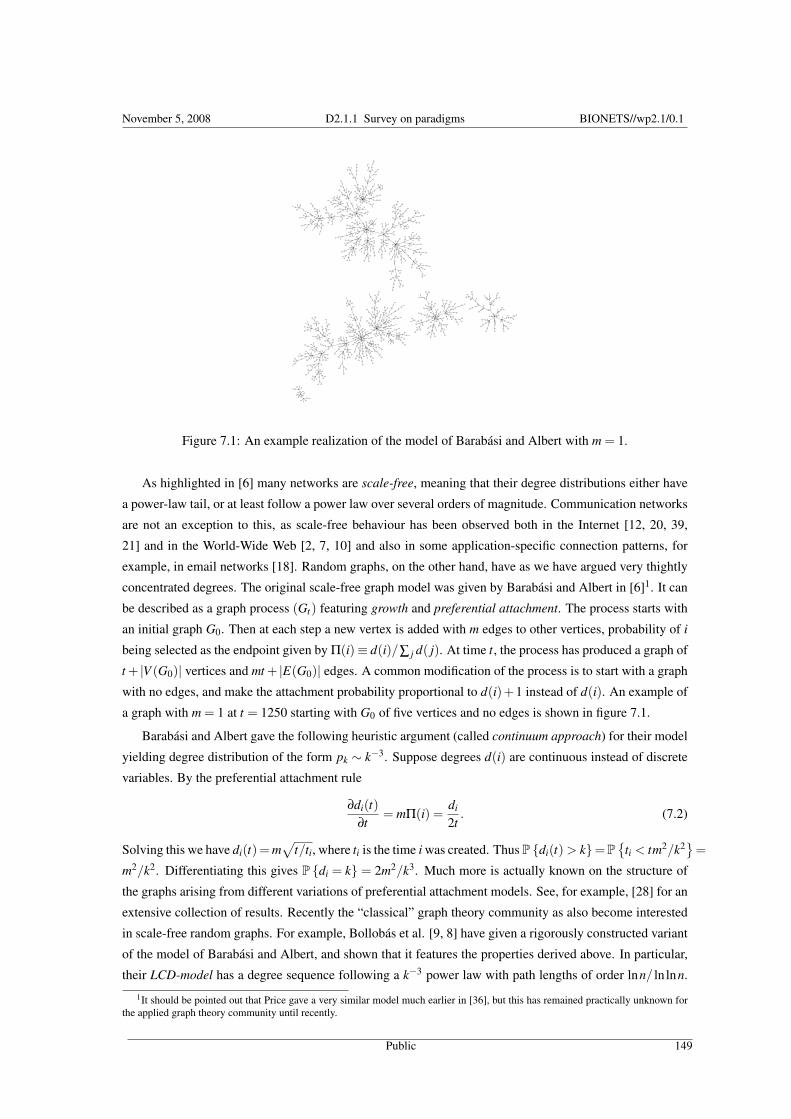
November 5, 2008 D2.1.1 Survey on paradigms BIONETS//wp2.1/0.1
Figure 7.1: An example realization of the model of Barabási and Albert with m = 1.
As highlighted in [6] many networks are scale-free, meaning that their degree distributions either have
a power-law tail, or at least follow a power law over several orders of magnitude. Communication networks
are not an exception to this, as scale-free behaviour has been observed both in the Internet [12, 20, 39,
21] and in the World-Wide Web [2, 7, 10] and also in some application-specific connection patterns, for
example, in email networks [18]. Random graphs, on the other hand, have as we have argued very thightly
concentrated degrees. The original scale-free graph model was given by Barabási and Albert in [6]1. It can
be described as a graph process (Gt) featuring growth and preferential attachment. The process starts with
an initial graph G0. Then at each step a new vertex is added with m edges to other vertices, probability of i
being selected as the endpoint given by Π(i)≡ d(i)/∑ j d( j). At time t, the process has produced a graph of
t + |V (G0)| vertices and mt + |E(G0)| edges. A common modification of the process is to start with a graph
with no edges, and make the attachment probability proportional to d(i)+1 instead of d(i). An example of
a graph with m = 1 at t = 1250 starting with G0 of five vertices and no edges is shown in figure 7.1.
Barabási and Albert gave the following heuristic argument (called continuum approach) for their model
yielding degree distribution of the form pk ∼ k−3. Suppose degrees d(i) are continuous instead of discrete
variables. By the preferential attachment rule
∂di(t)∂t
= mΠ(i) =di
2t. (7.2)
Solving this we have di(t)= m√
t/ti, where ti is the time i was created. Thus P di(t) > k=P
ti < tm2/k2
=
m2/k2. Differentiating this gives P di = k = 2m2/k3. Much more is actually known on the structure of
the graphs arising from different variations of preferential attachment models. See, for example, [28] for an
extensive collection of results. Recently the “classical” graph theory community as also become interested
in scale-free random graphs. For example, Bollobás et al. [9, 8] have given a rigorously constructed variant
of the model of Barabási and Albert, and shown that it features the properties derived above. In particular,
their LCD-model has a degree sequence following a k−3 power law with path lengths of order lnn/ ln lnn.
1It should be pointed out that Price gave a very similar model much earlier in [36], but this has remained practically unknown forthe applied graph theory community until recently.
Public 149
November 5, 2008 D2.1.1 Survey on paradigms BIONETS//wp2.1/0.1
See also [11] and [14].
While growth with variants of preferential attachment is by far the most studied combination in dynamic
network models, other types of dynamics have been studied as well. In [1] effects of local events (such as
edge rewirings) in combination with growth were studied. Effects of constraints such as maximum node
lifetimes and capacities have been studied by studied by several authors [16, 17, 4]. An interesting model
based on growth and copying has been given in [27, 29] to help to explain the structure of the World-Wide
Web graph. A salient feature of this model is that it can produce scale-free degree distributions for all values
of the power law exponent in [2,∞[. See [13] for further discussion on the copying models.
We conclude this section with a word of caution. While the models described above certainly replicate
many of the degree-related properties observed in communication networks, the case of modelling the large-
scale structure of the internet is by no means closed. Several features observed related to, for example, the
spectral structure and correlations in the node degrees are not properly covered by the preceding models. An
interesting take on the subject has been emerging from Doyle’s HOT programme (see [31, 3, 41]), trying
to explain the structure of the structure of the present-day networks as an outcome of a large collection
of local optimization procedures. Nevertheless, their applications have also been mainly confined to toy-
models, leaving ample room for further work on these matters.
7.3 Scale-free spatial structures
Relational structures are obviously of major importance in studying fixed networks. In wireless networks
the situation is, however, slightly different as the relational structure is purely a derived quantity, dependent
on the spatial structure of the network.
The spatial structure of the network can be modelled using the theory of point processes. Intuitively
point processes yield random point patterns in the same sense as random variables yield random numbers
(see the monographs of Karr [24] and Stoyan et al. [38] for an introduction). Technically a point process N
on a region A is defined as a random counting measure, that is, it assigns a random natural number N(Ai)
to any suitably regular subset Ai of A. The natural interpretation we are after is to think of N as a random
distribution of indistinguishable points in A, N(Ai) being the number of points lying in Ai. We can always
write N = ∑i εXi , where εx is the point mass at x (the measure equivalent to Dirac delta distribution), and
Xi is an A-valued random variable. The most fundamental point process is undoubtedly the Poisson point
process with intensity measure µ. It is defined by requiring independence of N(Ai) for all disjoint Ai and by
the law
PN(A) = k=µ(A)k
k!exp(−µ(A)).
Conditioned on the total number of points, the Poisson point process is used almost exclusively as the
model for node location distributions in the literature. It can clearly be thought of as the spatial analog of
the relational model of Erdos and Rényi. Unfortunately, as was the case above, the Poisson point process
cannot faithfully represent the rich structure present in the actually deployed wireless networks [37], making
its universal application problematic. We shall now have a more detailed look at the issues just alluded to,
with more detailed discussion available in [32].
The scale-free character of the location distributions of wireless nodes lies in spatial correlation func-
tions. Rigorously correlations of spatial processes is usually approached using Palm distributions. Here
Public 150
November 5, 2008 D2.1.1 Survey on paradigms BIONETS//wp2.1/0.1
we take a different road adopted in the applied spatial statistics community (astrophysicists in particular),
defining the pair correlation function via the definition of the joint probability density
dP = ν2(1+ξ(r))
dA1 dA2 (7.3)
of finding one point in each of the two area elements dA1 and dA2 with ν being the intensity of N. Clearly
if ξ≡ 0 no obvious correlation is present, as one would expect for, for example, the Poisson point process.
Positive values of ξ indicate positive correlations at the corresponding distance scales. The pair-correlation
function does not, of course, determine the distribution of a point process uniquely. An illustrative example
is the process of Baddeley and Silverman [5] having the same second-order structure as the Poisson point
processes while being structurally substantially different. Nevertheless, it has been found extremely power-
ful tool in a number of sciences and by the virtue of being straightforward to estimate numerically, warrants
close attention.
The definition of the pair-correlation function can, of course, be extended to the case of n-point correla-
tions. The definition analogous to (7.3) is given by the joint probability density
dP = νn(1+ξ(n)(r1,2,r1,3, . . . ,rn−1,n))
dA1 · · ·dAn,
of finding a point in each of the area elements dAi, where ri, j denotes the distance between area elements
dAi and dA j. For example, considering correlations up to the three-point case yields
dP = ν3(1+ξ(3)(r1,2,r1,3,r2,3))
dA1 dA2, dA3
= ν3(1+ξ(r1,2)+ξ(r1,3)+ξ(r2,3)+ζ(r1,2,r1,3,r2,3))
dA1 dA2, dA3,(7.4)
where ζ is the reduced three-point correlation function, expressing the residual three-point correlations that
do not arise from the two-point contributions directly.
To estimate the n-point correlations from a spatial data set a simple binning procedure can be utilised.
First, define the pair-counting function [26] by
Φr(x,y)≡ [r ≤ d(x,y)≤ r +∆], (7.5)
where d is the metric on E, and ∆ ∈ R+ is the width of the radial bin. Let D denote the collection of
observed point locations with n≡ |D|, and define the normalised observed pair counts by
DD(r) = ∑x∈D
∑y∈D
[x 6= y]Φr(x,y)/(n(n−1)). (7.6)
Further, let R be a realisation of a binomial point process of m points and define the normalised cross-pair
and random-pair counts by
DR(r) = ∑x∈D
∑y∈R
Φr(x,y)/(nm) (7.7)
and
RR(r) = ∑x∈R
∑y∈R
[x 6= y]Φr(x,y)/(m(m−1)), (7.8)
respectively.
Public 151
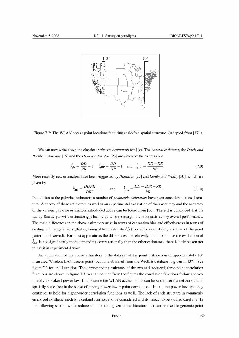
November 5, 2008 D2.1.1 Survey on paradigms BIONETS//wp2.1/0.1
-113° -80°
Figure 7.2: The WLAN access point locations featuring scale-free spatial structure. (Adapted from [37].)
We can now write down the classical pairwise estimators for ξ(r). The natural estimator, the Davis and
Peebles estimator [15] and the Hewett estimator [23] are given by the expressions
ξN ≡ DDRR
−1, ξDP ≡ DDDR
−1 and ξHe ≡ DD−DRRR
. (7.9)
More recently new estimators have been suggested by Hamilton [22] and Landy and Szalay [30], which are
given by
ξHa ≡ DDRRDR2 −1 and ξLS ≡ DD−2DR+RR
RR. (7.10)
In addition to the pairwise estimators a number of geometric estimators have been considered in the litera-
ture. A survey of these estimators as well as an experimental evaluation of their accuracy and the accuracy
of the various pairwise estimators introduced above can be found from [26]. There it is concluded that the
Landy-Szalay pairwise estimator ξLS has by quite some margin the most satisfactory overall performance.
The main differences in the above estimators arise in terms of estimation bias and effectiveness in terms of
dealing with edge effects (that is, being able to estimate ξ(r) correctly even if only a subset of the point
pattern is observed). For most applications the differences are relatively small, but since the evaluation of
ξLS is not significantly more demanding computationally than the other estimators, there is little reason not
to use it in experimental work.
An application of the above estimators to the data set of the point distribution of approximately 106
measured Wireless LAN access point locations obtained from the WiGLE database is given in [37]. See
figure 7.3 for an illustration. The corresponding estimates of the two and (reduced) three-point correlation
functions are shown in figure 7.3. As can be seen from the figures the correlation functions follow approx-
imately a (broken) power law. In this sense the WLAN access points can be said to form a network that is
spatially scale-free in the sense of having power-law n-point correlations. In fact the power-law tendency
continues to hold for higher-order correlation functions as well. The lack of such structure in commonly
employed synthetic models is certainly an issue to be considered and its impact to be studied carefully. In
the following section we introduce some models given in the literature that can be used to generate point
Public 152
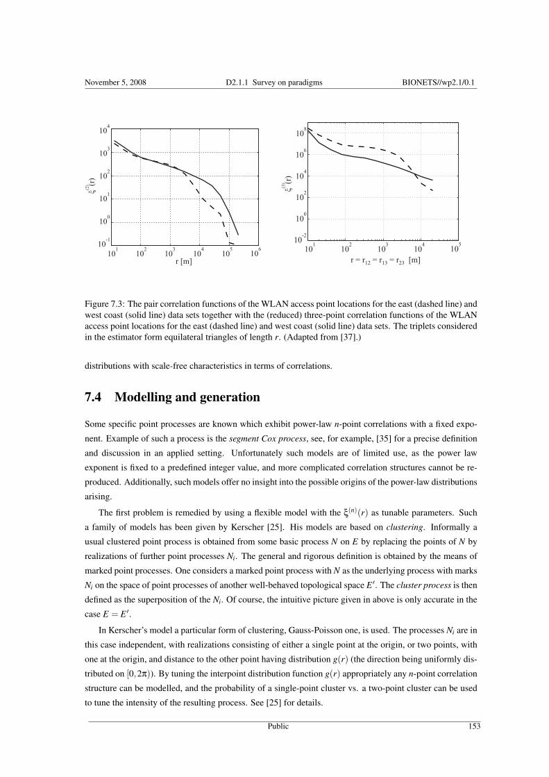
November 5, 2008 D2.1.1 Survey on paradigms BIONETS//wp2.1/0.1
104
100
101
102
103
10-1
ξ(r)
(2)
101
102
103
104
105
106
r [m]
102
108
10-2
ξ(r)
(3)
106
104
100
101
102
103
104
105
r = r = r = r [m]12 13 23
Figure 7.3: The pair correlation functions of the WLAN access point locations for the east (dashed line) andwest coast (solid line) data sets together with the (reduced) three-point correlation functions of the WLANaccess point locations for the east (dashed line) and west coast (solid line) data sets. The triplets consideredin the estimator form equilateral triangles of length r. (Adapted from [37].)
distributions with scale-free characteristics in terms of correlations.
7.4 Modelling and generation
Some specific point processes are known which exhibit power-law n-point correlations with a fixed expo-
nent. Example of such a process is the segment Cox process, see, for example, [35] for a precise definition
and discussion in an applied setting. Unfortunately such models are of limited use, as the power law
exponent is fixed to a predefined integer value, and more complicated correlation structures cannot be re-
produced. Additionally, such models offer no insight into the possible origins of the power-law distributions
arising.
The first problem is remedied by using a flexible model with the ξ(n)(r) as tunable parameters. Such
a family of models has been given by Kerscher [25]. His models are based on clustering. Informally a
usual clustered point process is obtained from some basic process N on E by replacing the points of N by
realizations of further point processes Ni. The general and rigorous definition is obtained by the means of
marked point processes. One considers a marked point process with N as the underlying process with marks
Ni on the space of point processes of another well-behaved topological space E ′. The cluster process is then
defined as the superposition of the Ni. Of course, the intuitive picture given in above is only accurate in the
case E = E ′.
In Kerscher’s model a particular form of clustering, Gauss-Poisson one, is used. The processes Ni are in
this case independent, with realizations consisting of either a single point at the origin, or two points, with
one at the origin, and distance to the other point having distribution g(r) (the direction being uniformly dis-
tributed on [0,2π)). By tuning the interpoint distribution function g(r) appropriately any n-point correlation
structure can be modelled, and the probability of a single-point cluster vs. a two-point cluster can be used
to tune the intensity of the resulting process. See [25] for details.
Public 153
November 5, 2008 D2.1.1 Survey on paradigms BIONETS//wp2.1/0.1
Another approach worth of consideration is the application of processes with explicit interactions be-
tween the points. Such processes could be considered as a spatial analog of the Albert-Barabasi model for
relational networks. The generic framework for such processes is given by the Gibbs models defined as
follows. Let us first consider a process N of n points Xi, defined on a bounded set E ⊂ Rd of volume A.
Suppose further that the law of N is given by a density function f : Rnd → [0,∞), that is,
P X1, . . . ,Xn ∈ B=∫
Bf (X1, . . . ,Xn)dX1 · · ·dXn. (7.11)
Now, to obtain a tractable family of models, we assume that to each configuration of points we assign a
numerical value called the energy or the Hamiltonian H(X1, . . . ,Xn). This approach is motivated by models
in physics in which such a quantity is often naturally defined. To obtain a more specific form for the
probability distribution we can now appeal to the maximum entropy principle, calling for maximisation of
the entropy of the system under the constraints obtained from observations or the modelling assumptions
made. By this assumption we now seek to find the law of N maximising the differential entropy
S =−∫
Enf (X1, . . . ,Xn) ln f (X1, . . . ,Xn)dX1 · · ·dXn (7.12)
under the constraint of constant H in expectation. This yields the density
f (X1, . . . ,Xn) = exp(−H(X1, . . . ,Xn)
)/Z, (7.13)
where the partition function Z is given by
Z =∫
Enexp
(−H(X1, . . . ,Xn))
dX1 · · ·dXn. (7.14)
The point process N defined in terms of the density f is called a Gibbs process, and is the spatial analog of
the maximum entropy graph models occasionally used to study scale-free network models [34].
As such the Gibbs model is of course still extremely general. Usually one assumes a simplified form
for the Hamiltonian H(X1, . . . ,Xn). A common choice considered in applications has been the pairwise
interaction model defined by
H(X1, . . . ,Xn) = a0 +n
∑i=1
ψ(Xi)+ ∑1≤i< j≤n
φ(Xi,X j) (7.15)
where ψ : Rd → R and φ : Rd ×Rd → R define the single-particle and pair contributions to H. Complex
interaction patterns and correlation structures can also be modelled by selecting a more complicated form
for the Hamiltonian. However, the simplest approach, and thus the one that should be covered in greater
detail first, would be to use the results from pair-correlation analysis of existing networks as a guide in
finding realistic pairwise interaction models. In the relational scale-free case the details have been worked
out by Park and Newman [33], but in the spatial case very little existing work is available, indicating the
need for further research.
7.5 Conclusions
While the structure of scale-free networks has been under intense investigation for almost a decade now the
field is still active and little signs of stagnation can be observed. Rather complete understanding of the so-
called configuration and preferential attachment models with scale-free degree distributions has emerged.
Public 154

November 5, 2008 D2.1.1 Survey on paradigms BIONETS//wp2.1/0.1
However, the realism and completeness of these models has recently been questioned, launching new re-
search avenues in the graph theory front. Comparatively less work has been done in characterizing networks
with significant spatial aspects in their structures, such as wireless networks of different kinds. In our work
we proposed the use of location correlations as a powerful paradigm. Initial results indicate that the metrics
chosen are able to convincingly distinguish between realizations of common artificial network models and
experimentally observed node locations. This distinction can now also be made quantitative in terms of
location correlations, and this quantification can be used as a basis for new network models.
Public 155

November 5, 2008 D2.1.1 Survey on paradigms BIONETS//wp2.1/0.1
Public 156
Bibliography
[1] R. Albert and A.L. Barabási. Topology of Evolving Networks: Local Events and Universality. Physi-
cal Review Letters, 85(24):5234–5237, 2000.
[2] R. Albert, H. Jeong, and A.L. Barabasi. Diameter of the World-Wide Web. Nature(London),
401(6749):130–131, 1999.
[3] D. Alderson, J.C. Doyle, L. Li, and W. Willinger. Towards a Theory of Scale-Free Graphs: Definition,
Properties, and Implications. Internet Math, 2(4):431–523, 2005.
[4] L.A.N. Amaral, A. Scala, M. Barthelemy, and HE Stanley. Classes of Small-World Networks. Pro-
ceedings of the National Academy of Sciences of the United States of America, 97(21):11149–11152,
2000.
[5] AJ Baddeley and BW Silverman. A Cautionary Example on the Use of Second-Order Methods for
Analyzing Point Patterns. Biometrics, 40(4):1089–1093, 1984.
[6] A.L. Barabási and R. Albert. Emergence of Scaling in Random Networks. Science, 286(5439):509–
512, 1999.
[7] A.L. Barabási, R. Albert, and H. Jeong. Scale-free characteristics of random networks: the topology
of the world-wide web. Physica A: Statistical Mechanics and its Applications, 281(1-4):69–77, 2000.
[8] B. Bollobás and O. Riordan. The Diameter of a Scale-Free Random Graph. Combinatorica, 24(1):5–
34, 2004.
[9] B. Bollobas, O. Riordan, J. Spencer, and G. Tusnady. The degree sequence of a scale-free random
graph process. Random Structures and Algorithms, 18(3):279–290, 2001.
[10] A. Broder, R. Kumar, F. Maghoul, P. Raghavan, S. Rajagopalan, R. Stata, A. Tomkins, and J. Wiener.
Graph structure in the Web. Computer Networks, 33(1-6):309–320, 2000.
[11] P.G. Buckley and D. Osthus. Popularity based random graph models leading to a scale-free degree
sequence. Discrete Mathematics, 282(1-3):53–68, 2004.
[12] Q. Chen, H. Chang, R. Govindan, and S. Jamin. The origin of power laws in Internet topologies
revisited. INFOCOM 2002. Twenty-First Annual Joint Conference of the IEEE Computer and Com-
munications Societies. Proceedings. IEEE, 2, 2002.
157

November 5, 2008 D2.1.1 Survey on paradigms BIONETS//wp2.1/0.1
[13] F. Chung, L. Lu, T.G. Dewey, and D.J. Galas. Duplication Models for Biological Networks. Journal
of Computational Biology, 10(5):677–687, 2003.
[14] C. Cooper and A. Frieze. A general model of web graphs. Random Structures and Algorithms,
22(3):311–335, 2003.
[15] M. Davis and PJE Peebles. A survey of galaxy redshifts. V- The two-point position and velocity
correlations. Astrophysical Journal, 267:465–482, 1983.
[16] SN Dorogovtsev and JFF Mendes. Evolution of networks with aging of sites. Physical Review E,
62(2):1842–1845, 2000.
[17] SN Dorogovtsev and JFF Mendes. Scaling behaviour of developing and decaying networks. Euro-
physics Letters, 52(1):33–39, 2000.
[18] H. Ebel, L.I. Mielsch, and S. Bornholdt. Scale-free topology of e-mail networks. Physical Review E,
66(3):35103, 2002.
[19] P. Erdös and A. Rényi. On the evolution of random graphs. Bulletin of the Institute of International
Statistics, 38:343–347, 1961.
[20] M. Faloutsos, P. Faloutsos, and C. Faloutsos. On power-law relationships of the Internet topology.
Comput. Commun. Rev, 29:251–263, 1999.
[21] R. Govindan and H. Tangmunarunkit. Heuristics for Internet map discovery. INFOCOM 2000. Nine-
teenth Annual Joint Conference of the IEEE Computer and Communications Societies. Proceedings.
IEEE, 3, 2000.
[22] AJS Hamilton. Toward better ways to measure the galaxy correlation function. Astrophysical Journal,
417(1):19–35, 1993.
[23] PC Hewett. The estimation of galaxy angular correlation functions. Royal Astronomical Society,
Monthly Notices,, 201:867–883, 1982.
[24] A. F. Karr. Point Processes and Their Statistical Inference. Marcel Dekker, 2nd edition, 1991.
[25] M. Kerscher. Constructing, characterizing, and simulating Gaussian and higher-order point distribu-
tions. Physical Review E, 64(5):56109, 2001.
[26] M. Kerscher, I. Szapudi, and A.S. Szalay. A Comparison of Estimators for the Two-Point Correlation
Function. The Astrophysical Journal, 535(1):L13–L16, 2000.
[27] J. Kleinberg, R. Kumar, P. Raghavan, S. Rajagopalan, and A. Tomkins. The web as a graph: Mea-
surements, models and methods. Proceedings of the International Conference on Combinatorics and
Computing, 6(1):6–1, 1999.
[28] PL Krapivsky and S. Redner. Organization of growing random networks. Physical Review E,
63(6):66123, 2001.
Public 158
November 5, 2008 D2.1.1 Survey on paradigms BIONETS//wp2.1/0.1
[29] R. Kumar, P. Raghavan, S. Rajagopalan, D. Sivakumar, A. Tomkins, and E. Upfal. Stochastic models
for the web graph. Proceedings of the 41st Annual Symposium on Foundations of Computer Science,
pages 57–65, 2000.
[30] S.D. Landy and A.S. Szalay. Bias and variance of angular correlation functions. The Astrophysical
Journal, 412:64, 1993.
[31] L. Li, D. Alderson, W. Willinger, and J. Doyle. A first-principles approach to understanding the
internet’s router-level topology. Proceedings of the 2004 conference on Applications, technologies,
architectures, and protocols for computer communications, pages 3–14, 2004.
[32] P. Mähönen, M. Petrova, and J. Riihijärvi. Applications of topology information for cognitive radios
and networks. In Proceedings of IEEE DySPAN 2007, April 2007.
[33] J. Park and MEJ Newman. Origin of degree correlations in the Internet and other networks. Physical
Review E, 68(2):26112, 2003.
[34] J. Park and MEJ Newman. Statistical mechanics of networks. Physical Review E, 70(6):66117, 2004.
[35] M.J. Pons-Borderia, V.J. Martinez, D. Stoyan, H. Stoyan, and E. Saar. Comparing Estimators of the
Galaxy Correlation Function. The Astrophysical Journal, 523(2):480–491, 1999.
[36] D.J.S. Price. A general theory of bibliometric and other cumulative advantage processes. J. Amer.
Soc. Inform. Sci, 27(5):292–306, 1976.
[37] J. Riihijärvi, P. Mähönen, and M. Rübsamen. Characterizing wireless networks by spatial correlations.
Communications Letters, IEEE, 11(1):37–39, 2007.
[38] D. Stoyan, W. S. Kendall, and J. Mecke. Stochastic geometry and its applications. Wiley, 1995.
[39] A. Vázquez, R. Pastor-Satorras, and A. Vespignani. Large-scale topological and dynamical properties
of the Internet. Physical Review E, 65(6):66130, 2002.
[40] DJ Watts and SH Strogatz. Collective dynamics of’small-world’networks. Nature, 393(6684):409–10,
1998.
[41] W. Willinger, D. Alderson, J.C. Doyle, and L. Li. More" normal" than normal: scaling distributions
and complex systems. Proceedings of the 36th conference on Winter simulation, pages 130–141, 2004.
Public 159

November 5, 2008 D2.1.1 Survey on paradigms BIONETS//wp2.1/0.1
Public 160

Chapter 8
Random matrix theory and freeprobabilityMerouane Debbah
8.1 Introduction
Random matrix theory have been a part of advanced multivariate statistical analysis since the end of the
1920’s. Random matrices were first proposed by Eugene Wigner in quantum mechanics where the statistics
of experimentally measured energy levels of nuclei were explained in terms of the eigenvalues of random
matrices. When Tsé [1] and Verdu [2] introduced nearly simultaneously random matrices in 1999 to model
uplink unfaded CDMA systems equipped with certain type of receivers, random matrix theory entered the
field of telecommunications. Until recently, in the field of information theory, simulations were widely
believed to be the only means to optimize a given network. However simulations had to be very intensive
and did not allow to single out parameters of interest easily. This changed when simultaneously in 1999, Tse
[1] and Verdú [2] introduced tools of Random Matrix Theory in order to analyse multi-user systems, in the
particular case of asymptotic performance of linear receivers for CDMA systems. They obtained explicit
expressions for various measures of interest such as capacity or Signal to Interference plus Noise Ratio
(SINR). Interestingly, it enables to single out the main parameters of interest that determine the performance
in numerous models of communication systems with more or less involved models of attenuation [1, 2, 3,
4, 5]. In addition, these asymptotic results provide good approximations for the practical finite size case,
as shown by simulations. A recent overview of Random Matrix Theory, centered on the applications to
Information Theory, is given in the book by Tulino and Verdú [6].
Random matrices were first studied by statistical physicists. One of the first studies was done in 1928
by Wishart [7]. He computed the probability density of v1vH1 + · · ·+ vnvH
n where vi are i.i.d. Gaussian
vectors. His results are among the few available on finite dimensional matrices. The typical question is
to characterize the distribution of (some of) the eigenvalues of random matrices. For finite matrix size
this distribution itself is usually random. The real interest in random matrices surged when non-random
limit distributions were derived for matrices whose dimensions tend to infinity, among others in 1955 by
Wigner [8] and in 1967 by Marchenko and Pastur [9]. The introduction of the (Cauchy-)Stieltjes transform
161
November 5, 2008 D2.1.1 Survey on paradigms BIONETS//wp2.1/0.1
[10, 11, 12] then enabled to derive distributions for more involved expressions: correlation among the
elements of the matrix, independant non-identically distributed elements, and sums and products of random
matrices. Random matrices are also particular non-commutative random variables.
Nowadays Random Matrix Theory is used in numerous domains, including but not limited to Riemann
hypothesis, stochastic differential equations, condensed matter physics, statistical physics, chaotic systems,
numerical linear algebra, neural networks, multivariate statistics, stock exchange analysis, and Information
Theory.
Another question that naturally arises in cognitive random networks [13] is the following: "From a set of
p noisy measurements, what can an intelligent device with n dimensions (time, frequency or space) extract
in terms of useful information on the network? Moreover, once this information has been extracted, how
can the terminal exploit (by capacity assessment, power allocation,...) that information?". It turns that these
questions have recently found answers in the realm of free deconvolution. Cognitive Random Networks
have been recently advocated as the next big evolution of wireless networks. The general framework is to
design self-organizing secure networks where terminals and base stations interact through cognitive sensing
capabilities. The complexity of these systems requires some sophisticated tools based on free probability
to make abstraction of the useless parameters. Free probability theory [14] is not a new tool but has grown
into an entire field of research since the pioneering work of Voiculescu in the 1980’s ([15, 16, 17, 18]).
However, the basic definitions of free probability are quite abstract and this has hinged a burden on its
actual practical use. The original goal was to introduce an analogy to independence in classical probability
that can be used for non-commutative random variables like matrices. These more general random variables
are elements in what is called a noncommutative probability space, which we only introduce partially as our
aim is to provide a more practical approach to these methods. Based on the moment/cumulant approach,
the free probability framework has been quite successfully applied recently in the pioneering works [19, 20]
to extract information (where information in wireless networks is related to the eigenvalues of the random
network) for very simple models i.e the case where one of the considered matrices is unitarily invariant. This
invariance has a special meaning in wireless networks and supposes that there is some kind of symmetry
in the problem to be analyzed. In this contribution, although focused on wireless communications, we
show that the cumulant/moment approach can be extended to more general models and provide explicit
algorithms to extract information (compute spectrums) on the network. In this paper, we give an explicit
relation between the spectrums of random matrices (M + N)(M + N)∗, MM∗ and NN∗, where M,N are
large rectangular independent random matrices, at least one of them having a distribution which is invariant
under multiplication, on any side, by any othogonal matrix. This had already been done ([21, 22, 23]), but
only in the case where M or N is gaussian.
8.2 Definitions and Notations
We consider the general case of two independent real rectangular random matrices M,N, both having size
n×p. We shall suppose that n, p tend to infinity in such a way that n/p tends to a real number λ ∈ [0,1].
We also suppose that at least one of these matrices has a distribution which is invariant by multiplication
on any side by any orthogonal matrix. At last, we suppose that the eigenvalue distributions of MM∗ and
NN∗ (i.e. the uniform distributions on their eigenvalues with multiplicity) both converge to non random
Public 162
November 5, 2008 D2.1.1 Survey on paradigms BIONETS//wp2.1/0.1
probability measures. From a historical and purely mathematical perspective, people have focused on these
types of random matrices because the invariance under actions of the orthogonal group is a – quite natural
– notion of isotropy. The Gram1 assumption was mainly due to the fact that the eigenvalues (which are real
and positive) are easier to characterize. From an engineering perspective, for a random network modeled by
a matrix M, the eigenvalues of MM∗ contain all the sufficient information to characterize the performance
of the system. In fact, the eigenvalues relate mainly to the energy of the system. We shall explain how one
can deduce, in a computational way, the limit eigenvalue distribution of (M + N)(M + N)∗ from the limit
eigenvalue distributions of MM∗ and NN∗. The underlying operation on probability measures is called the
rectangular free convolution with ratio λ and denoted by ¢λ in the literature ([24, 25, 26]). Our machinery
will also allow the inverse operation, called rectangular deconvolution with ratio λ: the derivation of the
eigenvalue distribution of MM∗ from the ones of (M+N)(M+N)∗ and NN∗.
We shall also review some classical results of free probability and show how (as long as moments of the
distributions are considered). One can, for A,B independent large square hermitian (or symmetric) random
matrices (under some general hypothesis that will be specified):
• Derive the eigenvalue distribution of A+B from the ones of A and B.
• Derive the eigenvalue distribution of AB or of A12 BA
12 from the ones of A and B.
The previous operations are known in the literature as free convolutions ([27]), and denoted respectively by
¢,¢.
We will also see how one can:
• Deduce the eigenvalue distribution of A from the ones of A+B and B.
• Deduce the eigenvalue distribution of A from the ones of AB or of A12 BA
12 and B.
These last operations are called free deconvolutions ([21]) and denoted respectively by ¯,r.
8.3 Information in random networks
In wireless intelligent random networks, devices are autonomous and should take optimal decisions based
on their sensing capabilities. Of particularly interest are information measures such as capacity, signal to
noise ratio, estimation of powers or even topology identification. Information measures are usually related
to the spectrum (eigenvalues) of the underlying network and not on the specific structure (eigenvectors).
This entails many simplifications that make free deconvolution a very appealing framework for the design
of these networks.
The fact that the spectrum of a stationary process is related to the information measure of the underlying
process dates back to Kolmogorov [28]. One can show that the entropy rate of a stationnary Gaussian
stochastic process can be expressed as:
H = log(πe)+1
2π
∫ π
−πlog(S( f ))d f ,
1For a matrix M, MM∗ is called the Gram matrix associated to M
Public 163
November 5, 2008 D2.1.1 Survey on paradigms BIONETS//wp2.1/0.1
where S is the spectral density of the process. Hence, if one knows the autocorrelation of the process, one
has therefore a full characterization of the information contained in the process. Moreover, as side result,
one can also show that the entropy rate is also related to the minimum mean squared error of the best esti-
mator of the process given the infinite past [29, 30]. This remarkable result is of main interest for wireless
communications as one can deduce one quantity from the other, especially as many receivers incorporate
an MMSE (Minimum Mean Square Error) component. These results show the central importance of the
autocorrelation function for Gaussian processes. In the discrete case when considering a random Gaussian
vector xi of size n, the entropy rate per dimension (or differential entropy) is given by:
H = log(πe)+1n
logdet(R)
= log(πe)+1n
n
∑i=1
log(λi), (8.1)
where R = E(xix∗i ) is the covariance and λi the associated eigenvalues. The covariance (and more precisely
its eigenvalues) carries therefore all the information of Gaussian networks. The Gaussianity of these net-
works is due to the fact that the noise, the channel and the signaling is very often Gaussian. Hence, in order
to get a reliable estimate of the rate (and in extension the capacity which is the difference between two
differential entropies or any other measure which involves performance criteria), one needs to compute the
eigenvalues of the covariance. For a number of observations p of the vector xi, i = 1, ..., p, the covariance
R is usually estimated by:
R =1p
p
∑i=1
xix∗i (8.2)
= R12 SS∗R
12 (8.3)
Here, S = [s1, ..,sp] is an n× p i.i.d zero mean Gaussian vector of variance 1p . It turns that in wireless
random networks, the number of samples p is of the same order as n. This is mainly due to the fact that
the network is highly mobile and the statistics are considered to be the same within a p number of sam-
ples, which restricts the use of classical asymptotic signal processing techniques. Therefore, information
retrieval must be performed within a window of limited samples. The main advantage of free deconvolution
techniques is that asymptotics "kick in" at a much earlier stage than other techniques available up to now.
The deconvolution framework comes here from the fact that we would like to invert equation (8.3) and
express R with respect to R. As we will show later on, this is not possible, however, one can compute the
eigenvalues of R knowing only the the eigenvalues of R (as the limiting eigenvalues of SS∗ are known to
be the Marchenko-Pastur law). This is mainly due to the fact that due to our invariance assumption on one
of the matrices (here SS∗), the eigenvector structure does not matter. Otherwise, it would have not been
possible. The invariance assumption "frees" in some sense one matrix from the other by "deconnecting"
their eigenspaces.
Public 164

November 5, 2008 D2.1.1 Survey on paradigms BIONETS//wp2.1/0.1
8.4 Eigenvalue distribution, joint eigenvalue distribution and mo-ments
8.4.1 Eigenvalue distribution and joint eigenvalue distribution
It is important to note at this stage what we mean by eigenvalue distribution. In general, one would like to
have the joint eigenvalue distribution of matrices or some marginal distribution with respect to the smallest
eigenvalue for example. It turns out that in wireless communications, functionals of the eigenvalues are
enough to characterize the measure of information or to retrieve information. Typically, as for the informa-
tion rate, one is interested in
Cn =1n
n
∑i=1
f (λi),
where f is a continous function (log(1 + x) for example)2. Note that Cn is a random variable (due to the
fact that the eigenvalues λi are random) and can be expressed as:
Cn =∫
f (λ)1n
δ(λ−λi)dλ (8.4)
=∫
f (λ)dρn(λ) (8.5)
We call here ρn the eigenvalue distribution which turns out to be nothing else than a projection of the
vector of eigenvalues [λ1, ...,λn] into a single quantity. It is therefore less explicit than the joint eigenvalue
distribution but contains all what is required for our problem. ρn is also a random variable but as the
dimension of the system grows, the behavior of the eigenvalue distribution becomes deterministic in many
cases. We will denote it ρ. Of course, other projections may also be of interest in other applications such as
the maximum of the vector [λ1, ...,λn].
8.4.2 Eigenvalue distribution and moments
Let us consider a probability measure ρ on the real line, which has moments of all order. We shall denote
by (mk(ρ) :=∫
tkdρ(t))k≥0 the sequence of its moments. A given sequence of moments mk,k ≥ 0 does
not uniquely determine the associated probability distribution. A trivial sufficient condition is the existence
of the moment generating function3. In any case, for computing the eigenvalue distribution, one needs to
determine the moments of all orders. However, once again, practical applications show that the limiting
eigenvalue distributions in wireless communications depends only a subset of parameters, typically:
dρ(λ) =1L
L
∑i=1
δ(λ−λi),
where L is small and is related to the problem of interest (class of users with a given power in multi-user
systems, number of scatterers in an environment, rank of the MIMO matrix in multiple antenna systems for
example).2In general, the function f should have other constraints (bounded) but for clarity reasons, we do not go into more details3A more sophisticated one is the Carleman condition, which states that the sequence characterizes a distribution if the following
holds:∞
∑i=1
m− 1
2i2i = ∞
Public 165

November 5, 2008 D2.1.1 Survey on paradigms BIONETS//wp2.1/0.1
In this case, the moments are related to the eigenvalues by the following relations:
mk(ρ) :=1L
L
∑i=1
λki . (8.6)
As detailed in [31, 19, 32], one needs only to compute L moments to retrieve the eigenvalues in equation
(8.6). This simplifies drastically the problems and favors a moment approach to the free deconvolution
framework rather than deriving the explicit spectrum.
The Newton-Girard Formulas [31] can be used to retrieve the eigenvalues from the moments. These
formulas state a relationship between the elementary symmetric polynomials
Π j(λ1, ...,λL) = ∑i1<···<i j≤L
λi1 · · ·λi j , (8.7)
and
Sp(λ1, ...,λL) =L
∑i=1
λpi
= L×mp(ρ)
through the recurrence relation
(−1)mmΠm(λ1, ...,λL)+ ∑m
k=1(−1)k+mSk(λ1, ...,λL)Πm−k(λ1, ...,λL) = 0.(8.8)
Interestingly, the characteristic polynomial
(λ−λ1) · · ·(λ−λL)
(which roots provides the eigenvalues of the associated matrix) can be fully characterized as its L− k
coefficient is given by: (−1)kΠk(λ1, ...,λL). As mp(ρ) (we will show later on how these quantities can be
computed) are known for 1≤ p≤ L, (8.8) can be used repeatedly to compute Πm(λ1, ...,λL), 1≤ m≤ L.
8.4.3 Information plus Noise model
Example (8.3) is unfortunately rarely encountered in practice in wireless communications. The signal of
interest si is usually distorted by a medium, given by mi = f (si) where f is any function. Moreover,
the received signal yi is altered by some additive noise ni (not necessarily Gaussian) but in many respect
unitarily invariant (due to the fact that all the dimensions have the same importance). In this case, the model
is known as the Information plus Noise model:
yi = mi +ni,
which can be rewritten in the following matrix form by stacking all the observations:
Y = M+N. (8.9)
The main challenge here is to infer on the eigenvalues of MM∗ when YY∗ and the eigenvalues of NN∗
are known (indeed, the noise can be measured by opening the receptor before the arrival of the signal
Public 166

November 5, 2008 D2.1.1 Survey on paradigms BIONETS//wp2.1/0.1
m). Once the spectrum of MM∗ has been computed (and depending on the function f ), one can get the
required information on the process si. Previous authors have addressed this problem through the Stieljes
transform [23] and other related methods for specific [33, 34, 35] models (typically, the case where N is i.i.d
Gaussian). In this work, we will show however that the cumulants/moment approach can be a very efficient
tool and provide implementable algorithms for a broader class of models.
8.5 Historical Perspective
Wigner [36] was interested in deriving the energy levels of nuclei. It turns out that energy levels are linked
to the Hamiltonian operator by the following Schrondinger equation:
Hφi = Eiφi
where
φi is the wave function
Ei is the energy level
H is the hamiltonian
Hence, the energy levels of the operator H is nothing else than the eigenvalues of the matrix represen-
tation of that operator. For a specific nuclei, finding the exact eigenvalues is a very complicated problem as
the number of interacting particles increase. The genuine idea of Wigner was to replace the exact matrix
by a random matrix having the same properties. Hence, in some cases, the matrix can be replaced by the
following hermitian random matrix where the upper diagonal elements are i.i.d generated with a binomial
distribution.
H =1√n
0 +1 +1 +1 −1 −1+1 0 −1 +1 +1 +1+1 −1 0 +1 +1 +1+1 +1 +1 0 +1 +1−1 +1 +1 +1 0 −1−1 +1 +1 +1 −1 0
It turns out as the dimension of the matrix increases, the eigenvalues of the matrix become more and
more predictable irrespective of the exact realization of the matrix. This striking result enabled to determine
the energy levels of many nuclei without considering the very specific nature of the interactions. In the
follwing, we will provide the different steps of the proof which are of interest for understanding the moment
approach.
8.6 Theoretical background
In the following, upper case and lower case boldface symbols will be used for matrices and column vec-
tors, respectively. (.)T will denote the transpose operator, (.)? conjugation and (.)H =((.)T
)? hermitian
transpose. E denotes the expectation operator.
Public 167

November 5, 2008 D2.1.1 Survey on paradigms BIONETS//wp2.1/0.1
−2.5 −2 −1.5 −1 −0.5 0 0.5 1 1.5 2 2.50
0.05
0.1
0.15
0.2
0.25
0.3
0.35
Figure 8.1: Semicircle law and simulation for a 512×512 Wigner matrix.
Definition 8.6.1 Let v = [v1, . . . ,vN ] be a vector. Its empirical distribution is the function FvN : R→ [0,1]
defined by:
FvN(x) =
1N
#vi ≤ x | i = 1 . . .N.
# corresponds to the cardinality operator. In other words, FvN(x) is the fraction of elements of v that are
inferior or equal to x. In particular, if v is the vector of eigenvalues of a matrix V, FvN is called the empirical
eigenvalue distribution of V.
A Wigner matrix is an N×N symmetric matrix H with diagonal entries zero and upper-triangle entries
i.i.d. zero mean and variance 1. As N → ∞, the empirical eigenvalue distribution of 1√N
H converges to the
semicircle law:
f (λ) =
1
2π√
4−λ2 if |λ| ≤ 20 if |λ| ≥ 2
The semicircle law is plotted in Fig. 8.1, as well as the plot obtained by tracing the histogram of the
eigenvalues of a single realization of a 512×512 Wigner matrix, with i.i.d. Gaussian N (0,1) distribution
of the upper-triangle entries. The semicircle already provides a good approximation of the eigenvalue dis-
tribution in the finite size case. Note that even though the nonzero entries are not bounded, the distribution
of the eigenvalues has a bounded support.
Wigner matrices have quite a constrained form, but it also possible to obtain results for a non-symmetric
matrix. If H is an N×N matrix with entries i.i.d. zero mean and variance 1, then the eigenvalues of 1√N
Hare uniformly distributed on the unit circle. This property is often referred to as Girko’s full circle law.
The full circle law is plotted in Fig. 8.2, as well as the plot of the eigenvalues of a single realization of
a 512×512 random matrix, with i.i.d. Gaussian N (0,1) distribution of the entries.
When non-square N×K matrices are under consideration, a common property of to ensure asymptotic
convergence of the distribution is that the ratio of the dimension KN be kept constant. One of the first
derivations of an explicit non-random limit distribution is due to Marchenko and Pastur. Let H be an N×K
matrix, with i.i.d. zero-mean complex entries with variance 1N and fourth moments O
(1
N2
). As K,N → ∞,
Public 168
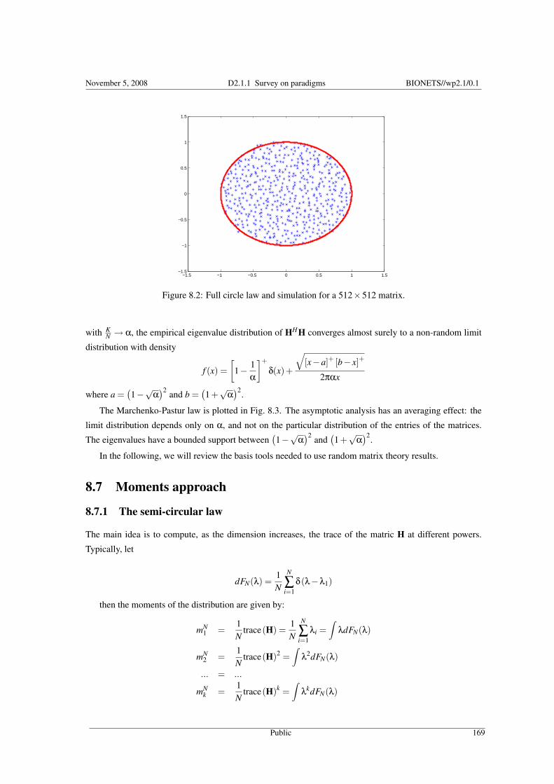
November 5, 2008 D2.1.1 Survey on paradigms BIONETS//wp2.1/0.1
−1.5 −1 −0.5 0 0.5 1 1.5−1.5
−1
−0.5
0
0.5
1
1.5
Figure 8.2: Full circle law and simulation for a 512×512 matrix.
with KN → α, the empirical eigenvalue distribution of HHH converges almost surely to a non-random limit
distribution with density
f (x) =[
1− 1α
]+
δ(x)+
√[x−a]+ [b− x]+
2παx
where a =(1−√α
)2 and b =(1+
√α)2.
The Marchenko-Pastur law is plotted in Fig. 8.3. The asymptotic analysis has an averaging effect: the
limit distribution depends only on α, and not on the particular distribution of the entries of the matrices.
The eigenvalues have a bounded support between(1−√α
)2 and(1+
√α)2.
In the following, we will review the basis tools needed to use random matrix theory results.
8.7 Moments approach
8.7.1 The semi-circular law
The main idea is to compute, as the dimension increases, the trace of the matric H at different powers.
Typically, let
dFN(λ) =1N
N
∑i=1
δ(λ−λ1)
then the moments of the distribution are given by:
mN1 =
1N
trace(H) =1N
N
∑i=1
λi =∫
λdFN(λ)
mN2 =
1N
trace(H)2 =∫
λ2dFN(λ)
... = ...
mNk =
1N
trace(H)k =∫
λkdFN(λ)
Public 169

November 5, 2008 D2.1.1 Survey on paradigms BIONETS//wp2.1/0.1
0 0.5 1 1.5 2 2.5 3 3.5 40
0.5
1
1.5
2
2.5
3
3.5
Figure 8.3: Marchenko-Pastur density function for α = 1,0.5,0.2.
Public 170
November 5, 2008 D2.1.1 Survey on paradigms BIONETS//wp2.1/0.1
Quite remarkably, as the dimension increases, the traces can be computed using combinatorial and non-
crossing partitions techniques. All the moments converge to what is known as the Catalan numbers In
particular, we have:
limN→∞
1N
Trace(H2k) =∫ 2
−2x2k f (x)dx
=1
k +1C2k
k
Note that since the semi-circle law is symmetric, the odd moments vanish. More importantly, the only
distribution which has all its moments equal to the Catalan number is known to be the semi-circular law
provided by:
f (x) =1
2π
√4− x2
with | x |≤ 2. Once can verify it directly by calculus based on recursion:
α2k =1π
∫ 2
−2x2k
√4− x2dx
= − 12π
∫ 2
−2
−x√4− x2
x2k−1(4− x2)dx
=1
2π
∫ 2
−2
√4− x2(x2k−1(4− x2))′dx
= 4(2k−1)α2k−2− (2k +1)α2k
In this way, the recursion is obtained:
α2k =2(2k−1)
k +1α2k−2
8.7.2 The marchenko-pastur Law
Let us give another example to understand the moments approach for a single random matrix. Suppose that
one is interested in the empirical eigenvalue distribution of HHH where H is N×K i.i.d Gaussian variance1N with K
N = α. In this case, in the same manner, the moments of this distribution are given by:
mN1 =
1N
trace(HHH)
=1N
N
∑i=1
λi → 1
mN2 =
1N
trace(HHH)2 =
1N
N
∑i=1
λ2i → 1+α
mN3 =
1N
trace(HHH)3 =
1N
N
∑i=1
λ3i → α2 +3α+1
It turns out that the only distribution which has the same moments is known to be the marchenko-pastur
Law.
Public 171
November 5, 2008 D2.1.1 Survey on paradigms BIONETS//wp2.1/0.1
Remark: In many cases, one would obviously think that the eigenvalues of
N
H
︸ ︷︷ ︸K
HH
when N → ∞, K/N → α are equal to one. Indeed, asymptotically, all the diagonal elements are equal to
one and the extra-diagonal elements are equal to zero. However, although the matrix "looks" like identity,
it is not identity. Indeed, there are N2 −N extra-diagonal terms which tend to zero at a rate of O( 1N2 ).
Therefore, the distance of the matrix to the identity matrix (in the froebenius norm sense) is not zero.
8.8 Freeness
The basic definitions of free probability are quite abstract, as the aim was to introduce an analogy to in-
dependence in classical probability that can be used for non-commutative random variables like matrices.
These more general random variables are elements in what is called a noncommutative probability space.
This can be defined by a pair (A,φ), where A is a unital ∗-algebra with unit I, and φ is a normalized (i.e.
φ(I) = 1) linear functional on A. The elements of A are called random variables. In all our examples, A will
consist of n× n matrices or random matrices. For matrices, φ will be the normalized trace trn, defined by
(for any a ∈ A)
trn(a) =1n
Tr(a) =1n
n
∑i=1
aii,
while for random matrices, φ will be the linear functional τn defined by
τn(a) =1n
n
∑i=1
E(aii) = E(trn(a)).
The unit in these ∗-algebras is the n× n identity matrix In. The noncommutative probability spaces
considered will all be tracial, i.e. φ satisfies the trace property φ(ab) = φ(ba). The analogy to independence
is called freeness:
Definition 8.8.1 A family of unital ∗-subalgebras (Ai)i∈I will be called a free family if
a j ∈ Ai j
i1 6= i2, i2 6= i3, · · · , in−1 6= inφ(a1) = φ(a2) = · · ·= φ(an) = 0
⇒ φ(a1 · · ·an) = 0. (8.10)
A family of random variables ai is called a free family if the algebras they generate form a free family.
One can note that the condition i1 6= in is not included in the definition of freeness. This may seem
strange since if φ is a trace and i1 = in, we can rearrange the terms so that two consecutive terms in (8.10)
come from the same algebra. If this rearranged term does not evaluate to zero through the definition of
freeness, the definition of freeness would be inconsistent. It is not hard to show that this small issue does
not cause an inconsistency problem. To see this, assume that (8.10) is satisfied for all indices where the
Public 172
November 5, 2008 D2.1.1 Survey on paradigms BIONETS//wp2.1/0.1
circularity condition i1 6= in is satisfied. We need to show that (8.10) also holds for indices where i1 = in.
By writing
ana1 = (ana1−φ(ana1)I)+φ(ana1)I = b1 +φ(ana1)I, (8.11)
we can express φ(a1 · · ·an)= φ(ana1a2 · · ·an−1) as a sum of the two terms φ(b1a2 · · ·an−1) and φ(ana1)φ(a2 · · ·an−1).
The first term is 0 by assumption, since φ(b1)= 0, b1 ∈Ain and in 6= in−1. The second term φ(ana1)φ(a2 · · ·an−1)
contributes with zero when i2 6= in−1 by assumption. If i2 = in−1, we use the same splitting as in (8.11) again,
but this time on φ(a2 · · ·an−1) = φ(an−1a2a3 · · ·an−2), to conclude that φ(a2 · · ·an−1) evaluates to zero un-
less i3 = in−2. Continuing in this way, we will eventually arrive at the term φ(an/2an/2+1) if n is even, or the
term φ(a(n+1)/2) if n is odd. The first of these is 0 since in/2 6= in/2+1, and the second is 0 by assumption.
Definition 8.8.2 We will say that a sequence of random variables an1,an2, ... in probability spaces (An,φn)
converge in distribution if, for any m1, ...,mr ∈Z, k1, ...,kr ∈1,2, ..., we have that the limit φn(am1nk1· · ·amr
nkr)
exists as n→ ∞. If these limits can be written as φ(am1k1· · ·amr
kr) for some noncommutative probability space
(A,φ) and free random variables a1,a2, ... ∈ (A,φ), we will say that the an1,an2, ... are asymptotically free.
Asymptotic freeness is a very useful concept for our purposes, since many types of random matrices ex-
hibit asymptotic freeness when their sizes get large. For instance, consider random matrices 1√n An1,
1√n An2, ...,
where the Ani are n× n with all entries independent and standard Gaussian (i.e. mean 0 and variance 1).
Then it is well-known [14] that the 1√n Ani are asymptotically free. The limit distribution of the 1√
n Ani in
this case is called circular, due to the asymptotic distribution of the eigenvalues of 1√n Ani: When n → ∞,
these get uniformly distributed inside the unit circle of the complex plane [37, 38]. (8.10) enables us to
calculate the mixed moments of free random variables a1 and a2. In particular, the moments of a1 +a2 and
a1a2 can be calculated. In order to calculate φ((a1 + a2)4), multiply out (a1 + a2)4, and use linearity and
(8.10) to calculate all φ(ai1ai2ai3 ai4) (i j = 1, 2). For example, to calculate φ(a1a2a1a2), write it as
φ(((a1−φ(a1)I)+φ(a1)I)((a2−φ(a2)I)+φ(a2)I)
((a1−φ(a1)I)+φ(a1)I)((a2−φ(a2)I)+φ(a2)I)),
and multiply it out as 16 terms. The term
φ((a1−φ(a1)I)(a2−φ(a2)I)
(a1−φ(a1)I)(a2−φ(a2)I))
is zero by (8.10). The term
φ((a1−φ(a1)I)φ(a2)I(a1−φ(a1)I)(a2−φ(a2)I))= φ(a2)φ((a1−φ(a1)I)(a1−φ(a1)I)(a2−φ(a2)I))
can be calculated by writing
b = (a1−φ(a1)I)(a1−φ(a1)I)
(which also is in the algebra generated by a1), setting
b = (b−φ(b)I)+φ(b)I,
and using (8.10) again. The same procedure can be followed for any mixed moments.
Public 173
November 5, 2008 D2.1.1 Survey on paradigms BIONETS//wp2.1/0.1
When the sequences of moments uniquely identify probability measures (which is the case for com-
pactly supported probability measures), the distributions of a1 + a2 and a1a2 give us two new probability
measures, which depend only on the probability measures associated with the moments of a1, a2. Therefore
we can define two operations on the set of probability measures: Additive free convolution
µ1 ¢µ2 (8.12)
for the sum of free random variables, and multiplicative free convolution
µ1 £µ2 (8.13)
for the product of free random variables. These operations can be used to predict the spectrum of sums or
products of asymptotically free random matrices. For instance, if a1n has an eigenvalue distribution which
approaches µ1 and a2n has an eigenvalue distribution which approaches µ2, one has that the eigenvalue
distribution of a1n +a2n approaches µ1 ¢µ2, so that µ1 ¢µ2 can be used as an eigenvalue predictor for large
matrices. Eigenvalue prediction for combinations of matrices is in general not possible, unless we have
some assumption on the eigenvector structures. Such an assumption which makes random matrices fit into
a free probability setting (and make therefore the random matrices free), is that of uniformly distributed
eigenvector structure (i.e. the eigenvectors point in some sense in all directions with equal probability).
We will also find it useful to introduce the concepts of additive and multiplicative free deconvolution:
Definition 8.8.3 Given probability measures µ and µ2. When there is a unique probability measure µ1 such
that
µ = µ1 ¢µ2, µ = µ1 £µ2 respectively,
we will write
µ1 = µ¯µ2, µ1 = µrµ2 respectively.
We say that µ1 is the additive free deconvolution (respectively multiplicative free deconvolution) of µ with
µ2.
It is noted that the symbols presented here for additive and multiplicative free deconvolution have not been
introduced in the literature previously. With additive free deconvolution, one can show that there always
is a unique µ1 such that µ = µ1 ¢ µ2. For multiplicative free deconvolution, a unique µ1 exists as long as
we assume non-vanishing first moments of the measures. This will always be the case for the measures we
consider.
Some probability measures appear as limits for large random matrices in many situations. One important
measure is the Marchenko Pastur law µc ([39] page 9), also known as the free Poisson distribution in free
probability. It is known that µc describes asymptotic eigenvalue distributions of Wishart matrices. Wishart
matrices have the form 1N RRH , where R is an n×N random matrix with independent standard Gaussian
entries. µc appears as limits of such when nN → c when n → ∞, Note that the Marchenko Pastur law can
also hold in the limit for non-gaussian entries.
Public 174

November 5, 2008 D2.1.1 Survey on paradigms BIONETS//wp2.1/0.1
8.9 Sum of two random matrices
8.9.1 Scalar case: X +Y
Let us consider two independent random variables X ,Y and suppose that we know the distribution of X +Y
and Y and would like to infer on the distribution of X . One way of doing that is to form the moment
generating functions
MX (s) = E(esX ), MX+Y (s) = E(es(X+Y )).
It is then immediate to see that
MX (s) = MX+Y (s)/MY (s).
The distribution of X can be recovered from MX (s). This task is however not always easy to perform
as the inversion formula does provide an explicit expression. Note also that the distribution of X +Y is the
convolution of the distribution of X with the distribution of Y . Here again, the expression is not always
straightforward to obtain. It is rather advantageous to express the independence in terms of moments of the
distributions or even cumulants which we denote by Ck the cumulant of order k. The cumulants are defined,
by the formula
Ck(X) :=∂n
∂tn |t=0log
(E
(etX))
.
They behave additively with respect to the convolution, i.e. we have, for all k ≥ 0,
Ck(X +Y ) = Ck(X)+Ck(Y ).
Recall that the moments of a random variable X are the numbers mn(X) =E(Xn), n≥ 1. It happens that
moments and cumulants of a random variable can easily be deduce from each other by the formula
∀n≥ 1,mn(X) =n
∑p=1
∑k1≥1,...,kp≥1k1+···+kp=n
Ck1(X) · · ·Ckp(X).
Thus the derivation of the law of X from the ones of X +Y and Y can be done by computing the
cumulants of X by the formula Ck(X) = Ck(X +Y )−Ck(X) and then deducing the moments of X from its
cumulants.
8.9.2 Additive free convolution ¢
Definition
It is has been proved by Voiculescu ([27]) that for An,Bn independent large n by n hermitian (or symmetric)
random matrices (both of them having iid entries, or one of them having a distribution which is invariant
under conjugation by any orthogonal matrix), if the eigenvalue distributions of An,Bn converge, as n tends
to infinity, to some probability measures µ,ν, then the eigenvalue distribution of An + Bn converges to a
probability measure which depends only on µ,ν, which is called the additive free convolution of µ and ν,
and which will be denoted by µ£ν.
Public 175

November 5, 2008 D2.1.1 Survey on paradigms BIONETS//wp2.1/0.1
Computation of µ¢ν by the moment/cumulants approach
Let us consider a probability measure ρ on the real line, which has moments of all order. We shall denote
its moments by mn(ρ) :=∫
tndρ(t), n≥ 1. (Note that in the case where ρ is the eigenvalue distribution
of a d× d matrix A, these moments can easily be computed by the formula: mn(ρ) = 1d Tr(An) ,where Tr
denotes the trace.) We shall associate to ρ another sequence of real numbers, (Kn(ρ))n≥1, called its free
cumulants. The sequences (mn(ρ)) and (Kn(ρ)) can be deduced one from each other by the fact that the
formal power series
Kρ(z) := ∑n≥1
Kn(ρ)zn and Mρ(z) := ∑n≥1
mn(ρ)zn (8.14)
are linked by the relation
Kρ(z(Mρ(z)+1)) = Mρ(z). (8.15)
Equivalently, for all n ≥ 1, the sequences (m0(ρ), . . . ,mn(ρ)) and (K1(ρ), . . . ,Kn(ρ)) can be deduced one
from each other via the relations
m0(ρ) = 1
mn(ρ) = Kn(ρ)+n−1
∑k=1
Kk(ρ) ∑l1,...,lk≥0
l1+···+lk=n−k
ml1(ρ) · · ·mlk(ρ)
for all n≥ 1.
The additive free convolution can be computed easily with the free cumulants via the following charac-
terization (see [40]).
þ For µ,ν compactly supported, µ¢ν is the only law m such that for all n≥ 1,
Kn(m) = Kn(µ)+Kn(ν).
8.9.3 The additive free deconvolution ¯
The moments/cumulants method can also be useful to implement the free additive deconvolution. The
additive free deconvolution of a measure m by a measure ν is (when it exists) the only measure µ such that
m = µ¢ν. In this case, µ is denoted by m¯ ν. By theorem 8.9.2, when it exists, m¯ ν is characterized by
the fact that for all n≥ 1, Kn(m¯ν) = Kn(m)−Kn(ν).
8.10 Product of two random matrices
8.10.1 Scalar case: XY
Suppose now that we are given two classical random variables X ,Y , assumed to be independent. How
do we find the distribution of X when only the distributions of XY and Y are given? The solution is
quite straightforward since E((XY )k) = E(Xk)E(Y k), so that E(Xk) = E((XY )k)/E(Y k). Hence, using the
moments approach, one has a neat algorithm to compute all the moments of the distribution. The case of
matrices is rather involved and is explained in the following.
Public 176
November 5, 2008 D2.1.1 Survey on paradigms BIONETS//wp2.1/0.1
8.10.2 The multiplicative free convolution £Definition
It is has been proved by Voiculescu ([27]) that for An,Bn independent large n by n positive hermitian (or
symmetric) random matrices (both of them having iid entries, or one of them having a distribution which is
invariant under conjugation by any orthogonal matrix), if the eigenvalue distributions of An,Bn converge,
as n tends to infinity, to some probability measures µ,ν, then the eigenvalue distribution of AnBn, which is
equal to the eigenvalue distribution of A12 BA
12 converges to a probability measure which depends only on
µ,ν, which is called the multiplicative free convolution of µ and ν, and which will be denoted by µ¢ν.
Computation of µ¢ν by the moment/cumulants approach
Let us consider a probability measure ρ on the [0,+∞), which is not the Dirac mass at zero and which has
moments of all order. We shall denote by (mn(ρ) :=∫
tndρ(t))n≥0 the sequence of its moments. We shall
associate to ρ another sequence of real numbers, (sn(ρ))n≥0, which are the coefficients of what is called its
S-transform. The sequences (mn(ρ)) and (sn(ρ)) can be deduced one from each other by the fact that the
formal power series
Sρ(z) := ∑n≥1
sn(ρ)zn−1 and Mρ(z) := ∑n≥1
mn(ρ)zn (8.16)
are linked by the relation
Mρ(z)Sρ(Mρ(z)) = z(1+Mρ(z)). (8.17)
Equivalently, for all n ≥ 1, the sequences (m1(ρ), . . . ,mn(ρ)) and (s1(ρ), . . . ,sn(ρ)) can be deduced one
from each other via the relations
m1(ρ)s1(ρ) = 1,
mn(ρ) = ∑n+1k=1 sk(ρ) ∑
l1,...,lk≥1l1+···+lk=n+1
ml1(ρ) · · ·mlk(ρ). (8.18)
rmq 8.10.1 Note that these equations allow computations which run faster than the ones already imple-
mented (e.g. [22]), because those ones are based on the computation of the coefficients sn via non crossing
partitions and the Kreweras complement, which use more machine time.
Example 8.10.2 As an example, it can easily be computed that for the Marchenko-Pastur law µλ, for all
n≥ 1, sn(µλ) = (−λ)n−1.
The multiplicative free convolution can be computed easily with the free cumulants via the following
characterization ([40]).
þ For µ,ν compactly supported probability measures on [0,∞), non of them being the Dirac mass at
zero, µ£ν is the only law m such that Sm = SµSν, i.e. such that for all n≥ 1,
sn(m) = ∑k,l≥1
k+l=n+1
sk(µ)sl(ν).
The algorithm for the computation of the spectrum of the product of two random matrices following
from this theorem has been implemented. It is presented in the following paragraph 8.10.3.
Public 177
November 5, 2008 D2.1.1 Survey on paradigms BIONETS//wp2.1/0.1
8.10.3 The multiplicative free deconvolution
The moments/cumulants method can also be useful to implement the multiplicative free deconvolution. The
multiplicative free deconvolution of a measure m by a measure ν is (when it exists) the only measure µ such
that m = µ£ν. In this case, µ is denoted by mrν. By theorem 8.10.2, when it exists, mrν is characterized
by the fact that for all n≥ 1,
sn(mrν)s1(ν) = sn(m)−n−1
∑k=1
sk(mrν)sn+1−k(ν).
Hence this operation, very useful to denoise a signal, can be implemented.
8.11 (M+N)(M+N)∗
8.11.1 Main result
In this section, we still consider two independent rectangular random matrices M,N, both having size n×p.
We shall suppose that n, p tend to infinity in such a way that n/p tends to a real number λ ∈ [0,1]. We also
suppose that at least one of these matrices has a distribution which is invariant by multiplication on both
sides by any orthogonal (or unitary, in the case where the matrices are not real but complex) matrix. At
last, we suppose that the eigenvalue distributions of MM∗ and NN∗ (i.e. the uniform distributions on there
eigenvalues with multiplicity) both converge to non random probability measures. Here, we shall denote by
respectively σ,τ the limit eigenvalue distributions of MM∗ and NN∗.
Note that in the previously presented results, the case of the limit eigenvalue distribution of (M +
N)(M + N)∗ has not been treated. The reason is that these results relay on the works of Voiculescu, who
"only" found out a general way to compute the limit normalized trace of product of independent square
random matrices with large dimension, which is all we need to compute the moments of the eigenvalue
distribution of either MM∗ + NN∗ or MM∗NN∗ (because in these expression, both M and N are always
followed by their adjoints), but which is not enough to compute the moments of the eigenvalue distribution
of (M+N)(M+N)∗. In a recent work ([24]), the first named author generalized Voiculescu’s work to rect-
angular random matrices, which allowed him to prove that, under the hypothesis made here, the eigenvalue
distribution of (M+N)(M+N)∗ converges to a probability measure which only depends on σ,τ and λ, and
will be denoted by σ¢+λ τ.
rmq 8.11.1 - The symmetric square root4 of the distribution σ ¢+λ τ is be called the rectangular free con-
volution with ratio λ of the symmetric square roots√
σ,√
τ of σ and τ, and denoted by√
σ ¢λ√
τ. The
operation ¢λ is, rather than ¢+λ , the one we introduced in [24]. It is essentially equivalent to ¢λ, as we
explain in the footnote below.
As for ¢, we shall see two ways to compute ¢λ: the first one is accomplished via the moments and is
easy to implement, and the second one relays on analytic functions and is practically working in very few
cases.4For any probability measure ρ on [0,∞), the symmetric square root of ρ, denoted by
√ρ, is the only symmetric probability measureon the real line which push-forward by the t 7→ t2 function is ρ. Note that ρ is completely determined by
√ρ, and vice versa. In thetheoretical paper [24], the use of symmetric measures was more appropriate, that’s why we chose to work with symmetric square rootsof measures. However, in the present paper, where we try to present how practically, matrices are working, we shall not symmetrizedistributions.
Public 178
November 5, 2008 D2.1.1 Survey on paradigms BIONETS//wp2.1/0.1
8.11.2 Computing ¢λ
We fix λ ∈ [0,1]. Let us consider a probability measure ρ on [0,+∞), which has moments of all orders.
We shall denote by (mn(ρ) :=∫
tndρ(t))n≥0 the sequence of its moments. We shall associate to ρ another
sequence of real numbers, (cn(ρ))n≥1, depending on λ, called its rectangular free cumulants5 with ratio
λ, defined by the fact that the sequences (mn(ρ)) and (cn(ρ)) can be deduced one from each other by the
relation
Cρ[z(λMρ2(z)+1)(Mρ2(z)+1)] = Mρ2(z) (8.19)
between the power series
Cρ(z) := ∑n≥1
cn(ρ)zn and Mρ2(z) := ∑n≥1
mn(ρ)zn. (8.20)
Equivalently, for all n≥ 1, the sequences (m0(ρ), . . . ,mn(ρ)) and (c1(ρ), . . . ,cn(ρ)) can be deduced one
from each other via the relations (involving an auxiliary sequence (m′0(ρ), . . . ,m′
n(ρ)))
m0(ρ) = m′0(ρ) = 1,
∀n≥ 1, m′n(ρ) = λmn(ρ),
∀n≥ 1, mn(ρ) =
cn(ρ)+n−1
∑k=1
ck(ρ) ∑l1,l′1,...,lk,l′k≥0
l1+l′1+···+lk+l′k=n−k
ml1(ρ)m′l′1(ρ) · · ·mlk(ρ)m′
l′k(ρ).
Example 8.11.2 As an example, it is proved in [41] that the law µλ has rectangular free cumulants with
ratio λ given by cn(µλ) = δn,1 for all n≥ 1.
The additive free convolution can be computed easily with the free cumulants via the following charac-
terization ([24]).
Theorem 8.11.3 For σ,τ compactly supported, σ ¢+λ τ is the only distribution m such that for all n ≥ 1,
cn(m) = cn(σ)+ cn(τ).
8.11.3 The rectangular free deconvolution
The moments/cumulants method can also be useful to implement the rectangular free deconvolution. The
rectangular free deconvolution with ratio λ of a probability measure m on [0,+∞) by a measure τ is (when
it exists) the only measure σ such that m = σ¢+λ τ. In this case, σ is denoted by m¯λ τ. By theorem 8.11.3,
when it exists, m¯λ τ is characterized by the fact that for all n≥ 1,
cn(m¯λ τ) = cn(m)− cn(τ).
Hence this operation, very useful to denoise a signal, can be implemented.
5Note that again, in [24], these numbers were not called rectangular free cumulants of ρ, but of its symmetrized square root.
Public 179

November 5, 2008 D2.1.1 Survey on paradigms BIONETS//wp2.1/0.1
8.11.4 Discussion
Case where λ = 0
It is proved in [24] that if λ = 0, then ¢+λ = ¢.
Concretely, it means that if M,N are independent n×p random matrices which dimensions n, p both
tend to infinity such that n/p→ 0, then (under the hypothesis that M or N is invariant, in distribution, under
multiplication by unitary matrices)
eigenvalue distribution((M+N)(M+N)∗)
' eigenvalue distribution(MM∗+NN∗).
Case where λ = 1
It is proved in [24] that if λ = 1, then for all σ,τ probability measures on [0,+∞), σ¢+λ τ is the push forward
by the function t 7→ t2 of the free convolution√
σ ¢√
τ of the symmetrized square roots√
σ,√
τ of σ and
τ.
An analytic tool: the rectangular R-transform
λ ∈ [0,1] is still fixed. For τ probability measure on [0,+∞), we shall define an analytic function Cτ(z) in a
neighborhood of zero (to be more precise, in a neighborhood of zero in C\R+) which, in the case where τis compactly supported, has the following series expansion:
Cτ(z) = ∑n≥1
cn(τ)zn. (8.21)
It implies, by theorem 8.11.3, that for all compactly supported probability measures σ,τ,
Cσ¢+λ τ(z) = Cσ(z)+Cτ(z). (8.22)
Hence the analytic transform ρ 7→Cρ somehow "linearizes" the binary operation ¢+λ on the set of probability
measures on [0,+∞). The analytic function τ 7→Cρ is called the rectangular R-transform6 with ratio λ of
ρ.
It happens, as we present it bellow, that for any probability measure ρ on [0,+∞), Cρ can be computed
in a direct way, without using the definition of (8.21), by the resolution of an equation.
Let us define Mρ(z) =∫
t∈R+zt
1−zt dρ(t). Then the analytic function Cρ is defined in a neighborhood of
zero (in C\R+) to be the solution of
Cρ[z(λMρ(z)+1)(Mρ(z)+1)] = Mρ(z). (8.23)
which tends to zero at zero.
To give a more explicit definition of Cρ, let us define
Hρ(z) = z(λMρ(z)+1)(Mρ(z)+1).
6Again, to make the notations of this paragraph coherent with the ones of the paper [24], where the rectangular machinery wasbuild, one needs to use the duality between measures on [0,+∞) and their symmetrized square roots, which are symmetric measureson the real line.
Public 180
November 5, 2008 D2.1.1 Survey on paradigms BIONETS//wp2.1/0.1
Then
Cρ(z) = U
(z
H−1ρ (z)
−1
)
with
U(z) =
−λ−1+((λ+1)2+4λz)
12
2λ if λ 6= 0,z if λ = 0,
where z 7→ z12 is the analytic version of the square root defined on C\R− such that 1
12 = 1 and H−1
ρ is the
inverse (in the sense of the composition) of the function Hρ.
To recover ρ from Cρ, one has to go the inverse way:
H−1ρ (z) =
z(λCρ(z)+1)(Cρ(z)+1)
and
Mρ(z) = U(
Hρ(z)z
−1)
,
from what one can easily recover ρ, via its Cauchy transform.
Note that all this method is working for non compactly supported probability measures, and that (8.22)
is valid for any pair of symmetric probability measures.
As for ¢ and £, analytic functions give us a new way to compute the multiplicative free convolution
of two symmetric probability measures τ,σ. However, as for ¢ and £, the operations which are necessary
in this method (the inversion of certain functions, the extension of certain analytic functions) are almost
always impossible to realize practically. However, in the following example, computations are possible.
Example 8.11.4 Suppose λ > 0. Then δ1 ¢+λ δ1 has support [(2−κ),(2 + κ)] with κ = 2(λ(2−λ))1/2 ∈
(0,2), and it admits a density with formula[κ2− (x−2)2
]1/2
πλx(4− x)(8.24)
on its support.
Concretely, it means that if A is an n×p matrix with ones on the diagonal and zeros everywhere else,
and U,V are random n×n, p×p orthogonal matrices with Haar distribution, then as n, p tend to infinity such
that n/p→ λ,
eigenvalue distribution(A+UAV)(A+UAV)∗ has density
'[κ2− (x−2)2
]1/2
πλx(4− x)on [2−κ,2+κ].
Indeed, [κ2−(x−2)2]1/2
πλx(4−x) is the density of the square of a random variable with density (8.24).
8.12 Examples in Wireless Random Networks
8.12.1 Topology information
The most simple example is the case where f is identity. This case is of practical interest when one per-
forms channel sounding measurements. The transmitter sends an impulse on a given band to sound the
Public 181
November 5, 2008 D2.1.1 Survey on paradigms BIONETS//wp2.1/0.1
environment. The channel response (or more precisely its power delay profile through the covariance of the
received signal) contains information on the structure of the environment. By appropriate ray tracing tech-
niques localization can be performed with a single receiver. The time-delayed channel impulse response
can be written as:
x(τ) =L
∑k=1
σkskg(τ− τk),
where sk are zero mean unit gaussian variables and σk are their associated variances (due to the topology),
L represent the total number of scatterers and g is the transmit filter. In the frequency domain, the received
vector for a given frequency fi in the presence of noise, can be written:
yi = xi +ni,
where xi = ∑Lk=1 skG( fi)e− j2π fiτk . In matrix form,
y = R12 s+n,
where R12 = Gθ . Here, G is a diagonal matrix with entries G( fi), θ is n×L matrix with entries e− j2π fiτk
and is a diagonal matrix with entries σk. s and n are respectively L×1 and n×1 zero mean unit variance
Gaussian vectors. The free deconvolution framework enables to infer on the L non-zero eigenvalues of Rand therefore σk as suggested in [19].
8.12.2 Capacity and SINR estimation
In the case of cognitive TDD (Time Division Duplex) MIMO systems (the transmitter and the receiver have
multi-antenna elements), the receiver would like to infer on the rate based only on the knowledge of the
variance of the noise σ2, but without any training systems and using only p samples. The TDD mode here
enables channel reciprocity by providing the same rate on both ends. The received signal can be written as:
yi = Hsi +ni,
where H is the n×n MIMO matrix. The information rate is given by [42]:
C = logdet(I+1
σ2 HH∗)
=n
∑i=1
log(1+λi). (8.25)
One can also be interested in the estimation of the SINR (Signal to Interference plus Noise Ratio) at the
output of the MMSE receiver (if Bit Error Rate requirements are imposed) which is asymptotically given
by [43]:
SINR =1n
trace(HH∗+σ2)−1
=1n
n
∑i=1
1λi +σ2
Public 182

November 5, 2008 D2.1.1 Survey on paradigms BIONETS//wp2.1/0.1
In both cases, the number of non-zero eigenvalues is also limited to L in general as the medium (matrix
H) provides only a finite number of degrees of freedom. One can compute these eigenvalues by using the
free deconvolution framework on YY∗.
8.12.3 Power estimation
In TDD heterogenous systems where a terminal is connected to several base stations, determining the power
of the signal received from each base station is important as it will induce the adequate rate splitting between
the different base stations. Suppose that each base station in the downlink has a given signature vector of
size n×1 hk (OFDM, CDMA) with random i.i.d components, the received signal can be written as:
y =L
∑k=1
hk√
Pksk +n
where Pk is the power received from each base station. L is the number of base stations, sk is the signal
transmitted by base station k and y and n are respectively the n× 1 received signal and additive noise. It
turns out here once again that one can infer on the powers Pk knowing only YY∗ as shown in [32].
8.13 The Stieljes Transform approach
Let µ be a probability measure on R. Its Stieljes transform:
Gµ(z) =∫ +∞
−∞
dµ(t)t− z
is defined on C/R. When z lies in the upper half-plane C+ = (z ∈ C : Im(z) > 0), the transform Gµ(z)
is an analytic function in C+ possessing the following properties:
Gµ(C+)⊂ C+ and | Gµ(z) |≤ 1Im(z)
Let µ be compactly supported. Then Gµ(z) is analytic in a neighborhood of ∞. Since (z− t)−1 =
∑∞k=0 tkz−k−1, it is obvious that Gµ(z) has the following expansion at z = ∞:
−Gµ(z) = z−1 +∞
∑k=0
mk(µ)z−k−1.
where mk(µ) =∫
tkdµ(t)(k ∈ Z+)
Writing z = x + iy, it is possible to recover µ from its Cauchy transform up to a factor . When µ is
absolutely continuous with respect to the Lebesgue measure, its density f(x) is given by:
f (x) = +1π
limy→0
ImGµ(x+ iy)
The random matrix theory in consideration here (see [44, 11] for more details) deals with the limiting
distribution of random Hermitian matrices of the form A+WDW H . Here, W (N×K),D(K×K),and A(N×N) are independent, with W containing i.i.d entries having finite second moments, T is diagonal with real
entries, A is Hermitian and K/N → α > 0 as N → ∞. The behavior is expressed in terms of the limiting
distribution function FA+WDW Hof the eigenvalues of A +WDW H (i.e FA+WDW H
(x) is the proportion of
Public 183

November 5, 2008 D2.1.1 Survey on paradigms BIONETS//wp2.1/0.1
eigenvalues of A+WDW H ≤ x). The remarkable result of random matrix theory is the convergence in some
sense, of FA+WDW H(x) to a non random F.
The papers vary in the assumption on T, W and A. We will only take here the case of interest.
Theorem 8.13.1 Let A be a N×N hermitian matrix, nonrandom, for which FA converges weakly as N →∞to a distribution function A. Let FD converges weakly to a nonrandom probability distribution function
denoted D. Suppose the entries of√
NW i.i.d for fixed N with unit variance (sum of the variances of the
real and imaginary parts in the complex case). Then the eigenvalue distribution of A +WDW H converges
weakly to a deterministic F. Its Stieljes transform G(z) satisfies the equation:
G(z) = GA
(z−α
∫ τdT(τ)1+ τG(z)
)(8.26)
8.13.1 A theoretical application example
We give hereafter the eigenvalue distribution of matrices defined by:
WN,KWHN,K +σ2I
where√
NWN,K is a N×K matrix with i.i.d entries with zero mean and variance one and N →∞ such asKN →α fixed. This example is intended to show to what extent (in terms of the matrix dimension) theoretical
and practical results fit. Moreover, we give the basic machinery that the reader can use to derive any limiting
eigenvalue distribution of matrices defined as in theorem 8.13.1.
Denote A = σ2I and D = IK,K . In this case, dA(x) = δ(x−σ2) and dD(x) = δ(x−1). Applying theorem
8.13.1, the following result is obtained:
G(z) = Gσ2I
(z−α
∫ τδ(τ−1)dτ1+ τG(z)
)(8.27)
= Gσ2I(z−α
1+G(z)) (8.28)
=∫ δ(σ2−λ)dλ
λ− z+ α1+G(z)
(8.29)
=1
σ2− z+ α1+G(z)
. (8.30)
Gσ2I(z) is the Cauchy transform of the eigenvalue distribution of matrix σ2I. The solution of the second
order equation 8.30 yields:
G(z) =1−α
2(σ2− z)− 1
2+− 1
2(σ2− z)
√((σ2− z+α−1)2 +4(σ2− z)).
The asymptotic eigenvalue distribution is therefore given by:
f (λ) =
[1−α]+δ(x)+ α
π(λ−σ2)
√λ−σ2− 1
4 (λ−σ2 +1−α)2 if σ2 +(√
α−1)2 ≤ λ≤ σ2 +(√
α+1)2
0 otherwise
Public 184
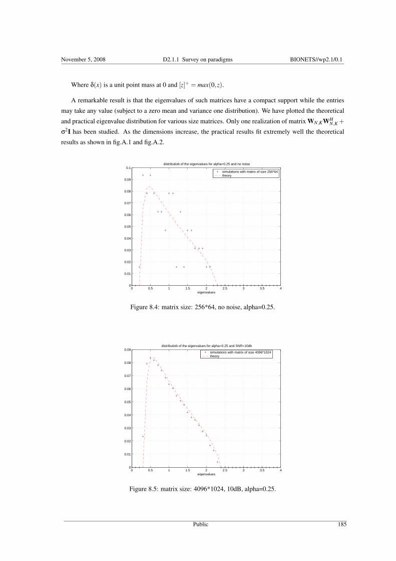
November 5, 2008 D2.1.1 Survey on paradigms BIONETS//wp2.1/0.1
Where δ(x) is a unit point mass at 0 and [z]+ = max(0,z).
A remarkable result is that the eigenvalues of such matrices have a compact support while the entries
may take any value (subject to a zero mean and variance one distribution). We have plotted the theoretical
and practical eigenvalue distribution for various size matrices. Only one realization of matrix WN,KWHN,K +
σ2I has been studied. As the dimensions increase, the practical results fit extremely well the theoretical
results as shown in fig.A.1 and fig.A.2.
0 0.5 1 1.5 2 2.5 3 3.5 40
0.01
0.02
0.03
0.04
0.05
0.06
0.07
0.08
0.09
0.1distributiob of the eigenvalues for alpha=0.25 and no noise
eigenvalues
simulations with matrix of size 256*64theory
Figure 8.4: matrix size: 256*64, no noise, alpha=0.25.
0 0.5 1 1.5 2 2.5 3 3.5 40
0.01
0.02
0.03
0.04
0.05
0.06
0.07
0.08
0.09distributiob of the eigenvalues for alpha=0.25 and SNR=10db
eigenvalues
simulations with matrix of size 4096*1024theory
Figure 8.5: matrix size: 4096*1024, 10dB, alpha=0.25.
Public 185

November 5, 2008 D2.1.1 Survey on paradigms BIONETS//wp2.1/0.1
8.13.2 A wireless communication example
Most of the information theoretic literature focuses on vector memoryless channels of the form:
Y = Hs+n. (8.31)
Eq. (8.31) covers the cases of a number of multiple access techniques, including but not limited to
Code Division Multiple Access (CDMA), Orthogonal Frequency Division Multiple Access (OFDMA) and
Multiple Input Multiple Output (MIMO). Under some assumptions, the capacity of the system is given by
1N
C =1N
logdet(
I+1
σ2 HHH)
=1N
N
∑i=1
log(
1+1
σ2 λi(HHH))
=∫
log(
1+1
σ2 λ)
1N
N
∑i=1
δ(λ−λi
(HHH))
dλ
=∫
log(
1+1
σ2 λ)
FHHH(λ)dλ.
Hence, as shown by the derivation above, the empirical eigenvalue distribution naturally appears in the
expression of the capacity. It also enables to derive several other performance measures of interest, such as
Signal to Interference plus Noise Ratio (SINR) or multiuser efficiency [2].
Unfortunately, the three laws plotted before are among the only known empirical eigenvalue distribu-
tions which have an explicit analytical expression. Generally, the limit distributions are given by an implicit
equation, and can only be computed numerically. It may look tiresome to first get the Stieltjes transform,
and then retrieve the empirical eigenvalue distribution using the inversion formula. Fortunately, there is a
way to circumvent this problem. One can observe that:
1N
C =∫
log(
1+1
σ2 λ)
FHHH(λ)dλ,
and differentiating according to σ2, we obtain
1N
∂C∂σ2 =
∫ − 1σ4 λ
1+ 1σ2 λ
FHHH(λ)dλ
=− 1σ2
∫ 1σ2 λ+1−1
1σ2 λ+1
FHHH(λ)dλ
=− 1σ2 +
∫ 1λ+σ2 FHHH
(λ)dλ
=− 1σ2 +mHHH (−σ2) .
Hence, finding the Stieltjes transform is often enough.
Public 186

Bibliography
[1] D.N.C Tse and S. Hanly, “Linear Multi-user Receiver: Effective Interference, Effective Bandwidth
and User Capacity,” pp. 641–657, Mar. 1999.
[2] S. Verdu and S. Shamai, “Spectral Efficiency of CDMA with Random Spreading,” pp. 622–640, Mar.
1999.
[3] J. Evans and D.N.C Tse, “Large System Performance of Linear Multiuser Receivers in Multipath
Fading Channels,” pp. 2059–2078, Sept. 2000.
[4] S. Shamai and S. Verdu, “The Impact of Frequency-Flat Fading on the Spectral Efficiency of CDMA,”
pp. 1302–1326, May 2001.
[5] A. Tulino, L. Li, and S. Verdu, “Spectral Efficiency of Multicarrier CDMA,” pp. 479 – 505, February
2005.
[6] A. M. Tulino and S. Verdu, Random Matrix Theory and Wireless Communications, Foundations and
Trends in Communications and Information Theory, NOW, The Essence of Knowledge, 1st edition,
2004.
[7] J. Wishart, “The Generalized Product Moment Distribution in Samples from a Normal Multivariate
Population,” Biometrika, vol. 20, no. A, pp. 32–52, 1928.
[8] E. Wigner, “Characteristic Vectors of Bordered Matrices with Infinite Dimensions,” Annals of Math-
ematics, vol. 62, pp. 546–564, 1955.
[9] V.A. Marchenko and L.A. Pastur, “Distribution of Eigenvalues for Some Sets of Random Matrices,”
Math USSR Sb., vol. 1, pp. 457–483, 1967.
[10] L.A. Pastur, “On the Spectrum of Random Matrices,” Teoret. Mat. Fiz., vol. 10, pp. 67–74, 1972.
[11] J.W. Silverstein and Z.D. Bai, “On the Empirical Distribution of Eigenvalues of a Class of Large
Dimensional Random Matrices,” J. Multivariate Anal., vol. 54, no. 2, pp. 175–192, 1995.
[12] V. L. Girko, “Theory of Random Determinants,” Kluwer Academic Publishers, Dordrecht, The
Netherlands, 1990.
[13] S. Haykin, “Cognitive Radio: Brain Empowered Wireless Communications,” Journal on Selected
Areas in Communications, vol. 23, pp. 201–220, 2005.
187
November 5, 2008 D2.1.1 Survey on paradigms BIONETS//wp2.1/0.1
[14] F. Hiai and D. Petz, The Semicircle Law, Free Random Variables and Entropy, American Mathematical
Society, 2000.
[15] D.V. Voiculescu, “Addition of certain non-commuting random variables,” J. Funct. Anal., vol. 66, pp.
323–335, 1986.
[16] D. V. Voiculescu, “Multiplication of certain noncommuting random variables,” J. Operator Theory,
vol. 18, no. 2, pp. 223–235, 1987.
[17] D.V. Voiculescu, “Circular and semicircular systems and free product factors,” vol. 92, 1990.
[18] D.V. Voiculescu, “Limit laws for random matrices and free products,” Inv. Math., vol. 104, pp.
201–220, 1991.
[19] Ø. Ryan and M. Debbah, “Free deconvolution for signal processing applications,” second round
review, IEEE Trans. on Information Theory, 2008, http://arxiv.org/abs/cs.IT/0701025.
[20] Ø. Ryan and M. Debbah, “Channel capacity estimation using free probability theory,” to appear,
2008, http://arxiv.org/abs/0707.3095.
[21] Ø. Ryan and M. Debbah, “Multiplicative free convolution and information-plus-noise
type matrices,” Planned for submission to Journal Of Functional Analysis, 2006,
http://www.ifi.uio.no/~oyvindry/multfreeconv.pdf.
[22] O. Ryan, “Implementation of free deconvolution,” Planned for submission to IEEE Transactions on
Signal Processing, 2006, http://www.ifi.uio.no/~oyvindry/freedeconvsigprocessing.pdf.
[23] B. Dozier and J.W. Silverstein, “On the empirical distribution of eigenvalues of large dimensional
information-plus-noise type matrices,” Submitted., 2004, http://www4.ncsu.edu/~jack/infnoise.pdf.
[24] Florent Benaych-Georges, “Rectangular random matrices, related convolution,” To appear in Proba-
bility Theory and Related Fields.
[25] Benaych-Georges Florent Guionnet Alice Belinschi, Serban, “Regularization by free additive convo-
lution, square and rectangular cases,” To appear in Complex Analysis and Operator Theory.
[26] Florent Benaych-Georges, “Infinitely divisible distributions for rectangular free convolution: classi-
fication and matricial interpretation,” Probab. Theory Related Fields, vol. 139, no. 1-2, pp. 143–189,
2007.
[27] D. V. Voiculescu, K. J. Dykema, and A. Nica, Free random variables, vol. 1 of CRM Monograph Se-
ries, American Mathematical Society, Providence, RI, 1992, A noncommutative probability approach
to free products with applications to random matrices, operator algebras and harmonic analysis on free
groups.
[28] T. Cover and J. Thomas, Elements of Information Theory, Wiley, 1991.
[29] D. Guo, S. Shamai, and S. Verdu, “Mutual information and minimum mean-square error in gaussian
channels,” vol. 51, no. 4, pp. 1261 – 1282, Apr. 2005.
Public 188

November 5, 2008 D2.1.1 Survey on paradigms BIONETS//wp2.1/0.1
[30] D. P. Palomar and S. Verdu, “Gradient of Mutual Information in Linear Vector Gaussian Channels,”
IEEE Trans. Information Theory, vol. 52, pp. 141–154, 2006.
[31] R. Seroul and D. O’Shea, Programming for Mathematicians, Springer.
[32] R. Couillet and M. Debbah, “Free deconvolution for ofdm multicell snr detection,” PIMRC 2008,
Cognitive Radio Workshop, Cannes, France, Sept, 2008.
[33] N.R. Rao and A. Edelman, “Free probability, sample covariance matrices and signal processing,”
ICASSP, pp. 1001–1004, 2006.
[34] N. Rao, J. Mingo, R. Speicher, and A. Edelman, “Statistical eigen-inference from large wishart ma-
trices,” http://front.math.ucdavis.edu/0701.5314, Jan, 2007.
[35] N. El. Karoui, “Spectrum estimation for large dimensional covariance matrices using random matrix
theory,” http://front.math.ucdavis.edu/0609.5418, Sept, 2006.
[36] E. Wigner, “On the distribution of roots of certain symmetric matrices,” The Annals of Mathematics,
vol. 67, pp. 325–327, 1958.
[37] V. L. Girko, “Circular Law,” Theory. Prob. Appl., pp. 694–706, vol. 29 1984.
[38] Z. D. Bai, “The Circle Law,” The Annals of Probability., pp. 494–529, 1997.
[39] A.M. Tulino and S. Verdo, Random Matrix Theory and Wireless Communications,
www.nowpublishers.com, 2004.
[40] Alexandru Nica and Roland Speicher, Lectures on the combinatorics of free probability, vol. 335 of
London Mathematical Society Lecture Note Series, Cambridge University Press, Cambridge, 2006.
[41] Florent Benaych-Georges, “Infinitely divisible distributions for rectangular free convolution: classi-
fication and matricial interpretation,” Probab. Theory Related Fields, vol. 139, no. 1-2, pp. 143–189,
2007.
[42] E. Telatar, “Capacity of Multi-Antenna Gaussian Channels,” Eur. Trans. Telecomm. ETT, vol. 10, no.
6, pp. 585–596, Nov. 1999.
[43] D. Tse and S. Hanly, “Linear multiuser receivers: Effective interference, effective bandwidth and user
capacity,” IEEE Transactions on Information Theory, vol. 45, no. 2, pp. 641–657, 1999.
[44] V.A. Marchenko and L.A. Pastur, “Distribution of Eigenvalues for Some Sets of Random Matrices,”
Math USSR Sb., vol. 1, pp. 457–483, 1967.
:
Public 189

November 5, 2008 D2.1.1 Survey on paradigms BIONETS//wp2.1/0.1
Public 190
Chapter 9
Tools from Physics and Road-trafficEngineering for Dense Ad-hocNetworksE. Altman, P. Bernhard, M. Debbah, A. Silva
Abstract We consider massively dense ad-hoc networks and study their continuum limits as the node density increases
and as the graph providing the available routes becomes a continuous area with location and congestion dependent costs.
We study both the global optimal solution as well as the non-cooperative routing problem among a large population
of users where each user seeks a path from its source to its destination so as to minimize its individual cost. We
seek for a (continuum version of the) Wardrop equilibrium. We first show how to derive meaningful cost models as
a function of the scaling properties of the capacity of the network and of the density of nodes. We present various
solution methodologies for the problem: (1) the viscosity solution of the Hamilton-Bellman-Jacobi equation, for the
global optimization problem, (2) a method based on Green Theorem for the least cost problem of an individual, and (3)
a solution of the Wardrop equilibrium problem using a transformation into an equivalent global optimization problem.
9.1 Introduction
In the design and analysis of wireless networks, researchers frequently stumble on the scalability problem
that can be summarized in the following sentence: “As the number of nodes in the network increases,
problems become harder to solve” [26]. The sentence takes its meaning from several issues. Some examples
are the following:
• In Routing: As the network size increases, routes consists of an increasing number of nodes, and so
they are increasingly susceptible to node mobility and channel fading [22].
• In Transmission Scheduling: The determination of the maximum number of non-conflicting trans-
missions in a graph is a NP-complete problem [29].
• In Capacity of Wireless Networks: As the number of nodes increases, the determination of the precise
capacity becomes an intractable problem.
191
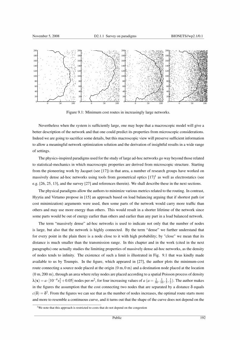
November 5, 2008 D2.1.1 Survey on paradigms BIONETS//wp2.1/0.1
0 50 1000
20
40
60
80
100
120
140
160
180
200
0 50 1000
20
40
60
80
100
120
140
160
180
200
0 50 1000
20
40
60
80
100
120
140
160
180
200
0 50 1000
20
40
60
80
100
120
140
160
180
200
Figure 9.1: Minimum cost routes in increasingly large networks.
Nevertheless when the system is sufficiently large, one may hope that a macroscopic model will give a
better description of the network and that one could predict its properties from microscopic considerations.
Indeed we are going to sacrifice some details, but this macroscopic view will preserve sufficient information
to allow a meaningful network optimization solution and the derivation of insightful results in a wide range
of settings.
The physics-inspired paradigms used for the study of large ad-hoc networks go way beyond those related
to statistical-mechanics in which macroscopic properties are derived from microscopic structure. Starting
from the pioneering work by Jacquet (see [17]) in that area, a number of research groups have worked on
massively dense ad-hoc networks using tools from geometrical optics [17]1 as well as electrostatics (see
e.g. [26, 25, 13], and the survey [27] and references therein). We shall describe these in the next sections.
The physical paradigms allow the authors to minimize various metrics related to the routing. In contrast,
Hyytia and Virtamo propose in [15] an approach based on load balancing arguing that if shortest path (or
cost minimization) arguments were used, then some parts of the network would carry more traffic than
others and may use more energy than others. This would result in a shorter lifetime of the network since
some parts would be out of energy earlier than others and earlier than any part in a load balanced network.
The term “massively dense” ad-hoc networks is used to indicate not only that the number of nodes
is large, but also that the network is highly connected. By the term “dense” we further understand that
for every point in the plain there is a node close to it with high probability; by "close" we mean that its
distance is much smaller than the transmission range. In this chapter and in the work (cited in the next
paragraphs) one actually studies the limitting properties of massively dense ad-hoc networks, as the density
of nodes tends to infinity. The existence of such a limit is illustrated in Fig. 9.1 that was kindly made
available to us by Toumpis. In the figure, which appeared in [27], the author plots the minimum-cost
route connecting a source node placed at the origin (0 m,0 m) and a destination node placed at the location
(0 m,200 m), through an area where relay nodes are placed according to a spatial Poisson process of density
λ(x) = a · [10−4x21 +0.05] nodes per m2, for four increasing values of a (a = 1
30 , 110 , 1
5 , 12 ). The author makes
in the figures the assumption that the cost connecting two nodes that are separated by a distance δ equals
c(δ) = δ2. From the figures we can see that as the number of nodes increases, the optimal route starts more
and more to resemble a continuous curve, and it turns out that the shape of the curve does not depend on the
1We note that this approach is restricted to costs that do not depend on the congestion
Public 192
November 5, 2008 D2.1.1 Survey on paradigms BIONETS//wp2.1/0.1
precise node placement, but only on the node density function λ(x) and the cost-versus-distance function
c(δ).
The development of the original theory of routing in massively dense networks among the community of
ad-hoc networks has emerged in a complete independent way of the existing theory of routing in massively
dense networks which had been developed within the community of road traffic engineers. Indeed, this
approach had already been introduced in 1952 by Wardrop [30] and by Beckmann [4] and is still an active
research area among that community, see [6, 7, 14, 16, 32] and references therein. We combine in this
chapter various approaches from this area as well as from optimal control theory in order to formulate
models for routing in massively dense networks. We further propose simple novel approach to that problem
using a classical device of 2-D. singular optimal control [19] based on Green’s formula to obtain a simple
characterization of least cost paths of individual packets. We end the chapter by a numerical example for
computing an equilibrium.
We consider in this chapter static networks (say sensor networks) characterized by communications
through horizontally and vertically oriented directional antennas. The use of directional antennas allows
one to save energy and to use it in an efficient way which may result in a longer life time of the network.
The structure of this chapter is as follows. We begin by presenting models for costs relevant to op-
timization models in routing or to node assignment. We then formulate the global optimization problem
and the individual optimization one with a focus on the directional antennas scenario. We provide several
approaches to obtain both qualitative characterization as well as quantitative solutions to the problems.
9.2 Determining routing costs in dense ad-hoc networks
In optimizing a routing protocol in ad-hoc networks, or in optimizing the placement of nodes, one of the
starting points is the determination of the cost function. To determine it, we need a detailed specification of
the network which includes the following:
• A model for the placement of nodes in the network.
• A forward rule that nodes will use to select the next hop of a packet.
• A model for the cost incurred in one hop, i.e. for transmitting a packet to an intermediate node.
Below we present several ways of choosing cost functions.
9.2.1 Costs derived from capacity scaling
Many models have been proposed in the literature that show how the transport capacity scales with the
number of nodes n or with their density λ. Assume that we use a protocol that provides a transport capacity
of the order of f (λ) at some region in which the density of nodes is λ. A typical cost (see e.g. [25]) at a
neighborhood of x is the density of nodes required there to carry a given flow. Assuming that a flow2 T(x)
is assigned through a neighborhood of x, the cost is taken to be
c(x,T(x)) = f−1(|T(x)|) (9.1)2We denote with bold font the vectors.
Public 193

November 5, 2008 D2.1.1 Survey on paradigms BIONETS//wp2.1/0.1
where | · | represents the norm of a vector.
Examples for f :
• Using a network theoretic approach based on multi-hop communication, Gupta and Kumar prove
in [12] that the throughput of the system that can be transported by the network when the nodes
are optimally located is Ω(√
λ), and when the nodes are randomly located this throughput becomes
Ω(√
λ√logλ
). Using percolation theory, the authors of [9] have shown that in the randomly located set
the same Ω(√
λ) can be achieved.
• Baccelli, Blaszczyszyn and Mühlethaler introduce in [2] an access scheme, MSR (Multi-hop Spatial
Reuse Aloha), reaching the Gupta and Kumar bound O(√
λ) which does not require prior knowledge
of the node density.
• A protocol introduced by Tse and Glosglauser [10] has a capacity that scales as O(λ). However, it
does not fall directly within the class of massively dense ad-hoc networks and indeed, it relies on
mobility and on relaying for handling disconnectivity.
We conclude that for the model of Gupta and Kumar with either the optimal location or the random location
approaches, as well as for the MSR protocol with a Poisson distribution of nodes, we obtain a quadratic
cost of the form
c(T(x)) = k|T(x)|2 (9.2)
This follows from (9.1) as f (x) behaves like√
x so its inverse is quadratic.
9.2.2 Congestion independent routing
A metric often used in the Internet for determining routing is the number of hops, which routing protocol
try to minimize. The number of hops is proportional to the expected delay along the path in the context
of ad-hoc networks, in case that the queuing delay is negligible with respect to the transmission delay over
each hop. This criterion is insensitive to interference or congestion. We assume that it depends only on the
transmission range. We describe various cost criteria that can be formulated with this approach.
• If the range were constant then the cost density c(x) is constant so that the cost of a path is its length
in meters. The routing then follows a shortest path selection.
• Let us assume that the range R(x) depends on local radio conditions at a point x (for example, if it
is influenced by weather conditions) but not on interference. The latter is justified when dedicated
orthogonal channels (e.g. in time or frequency) can be allocated to traffic flows that would otherwise
interfere with each other. Then determining the routing becomes a path cost minimization problem.
We further assume, as in Gupta and Kumar, that the range is scaled to go to 0 as the total density λ of
nodes grows to infinity. More precisely, let us consider a scaling of the range such that the following
limit exists:
r(x) := limλ→∞
Rλ(x)λ
Then in the dense limit, the fraction of nodes that participate in forwarding packets along a path is
1/r(x) and the path cost is the integral of this density along the path.
Public 194
November 5, 2008 D2.1.1 Survey on paradigms BIONETS//wp2.1/0.1
• The influence of varying radio conditions on the range can be eliminated using power control that can
equalize the hop distance.
9.2.3 Costs related to energy consumption
In the absence of capacity constraints, the cost can represent energy consumption. In a general multi-hop
ad-hoc network, the hop distance can be optimized so as to minimize the energy consumption. Even within
a single cell of 802.11 IEEE wireless LAN one can improve the energy consumption by using multiple
hops, as it has been shown not to be efficient in terms of energy consumption to use a single hop [20].
Alternatively, the cost can take into account the scaling of the nodes (as we had in Subsection 9.2.1)
that is obtained when there are energy constraints. As an example, assuming random deployment of nodes,
where each node has data to send to another randomly selected node, the capacity (in bits per Joule) has the
form f (λ) = Ω((λ/ logλ)(q−1)/2
)where q is the path-loss, see [21]. The cost is then obtained using (9.1).
9.3 Preliminary
In the work of Toumpis et al. ([26, 25, 13, 28, 27]), the authors address the problem of the optimal deploy-
ment of Wireless Sensor Networks by a parallel with Electrostatic.
Consider in the two dimensional plane X1 ×X2, the continuous information density function ρ(x),
measured in bps/m2, such that at locations x where ρ(x) > 0 there is a distributed data source such that the
rate with which information is created in an infinitesimal area of size dΩ centered at x is ρ(x)dΩ. Similarly,
at locations x where ρ(x) < 0 there is a distributed data sink such that the rate with which information is
absorbed by an infinitesimal area of size dΩ, centered at point x, is equal to −ρ(x)dΩ.
The total rate at which sinks must absorb data is the same as the total rate which the data is created at
the sources, i.e. ∫
X1×X2
ρ(x)dS = 0.
Next we present the flow conservation condition (see e.g. [25, 6] for more details). For information
to be conserved over a domain Ω0 of arbitrary shape on the X1 ×X2 plane, (but with smooth boundary)
it is necessary that the rate with which information is created in the area is equal to the rate with which
information is leaving the area, i.e∫
Ω0
ρ(x)dx =∮
∂Ω0
[T(x) ·n(x)]d`
The integral on the left is the surface integral of ρ(x) over Ω0. The integral on the right is the path
integral of the inner product T ·n over the curve ∂Ω0. The vector n(x) is the unit normal vector to ∂Ω0 at
the boundary point x ∈ ∂Ω0 and pointing outwards. The function T(x) ·n(x) measured in bps/m2 is equal
at the rate with which information is leaving the domain Ω0 per unit length of boundary at the boundary
point x.
This holding for any (smooth) domain Ω0, it follows that necessarily
∇ ·T(x) :=∂T1(x)
∂x1+
∂T2(x)∂x2
= ρ(x), (9.3)
Public 195

November 5, 2008 D2.1.1 Survey on paradigms BIONETS//wp2.1/0.1
where “∇·” is the divergence operator.
Extension to multi-class The work on massively dense ad-hoc networks considered a single class of
traffic. In the geometrical optics approach it corresponded to demand from a point a to a point b. In the
electrostatic case it corresponded to a set of origins and a set of destinations where traffic from any origin
point could go to any destination point. The analogy to positive and negative charges in electrostatics may
limit the perspectives of multi-class problems where traffic from distinct origin sets has to be routed to
distinct destination sets.
The model based on geometrical optics can directly be extended to include multiple classes as there are
no elements in the model that suggest coupling between classes. This is due in particular to the fact that the
cost density has been assumed to depend only on the density of the mobiles and not on the density of the
flows.
In contrast, the cost in the model based on electrostatics is assumed to depend both on the location
as well as on the local flow density. It thus models more complex interactions that would occur if we
considered the case of ν traffic classes. Extending the relation (9.3) to the multi-class case, we have traffic
conservation at each point in space to each traffic class as expressed in the following:
∇ ·T j(x) = ρ j(x), ∀x ∈Ω. (9.4)
The function T j is the flow distribution of class j and ρ j corresponds to the distribution of the external
sources and/or sinks.
Let T(x) be the total flow vector at point x ∈Ω. A generic multi-class optimization problem would then
be: minimize Z over the flow distributions T ji
Z =∫
Ωg(x,T(x))dx1dx2 subject to ∇ ·T j(x) = ρ j(x), j = 1, ...,ν ∀x ∈Ω. (9.5)
9.4 Directional Antennas and Global Optimization
Unlike the previous work that we described on massively dense ad-hoc networks, we introduce a model that
uses directional antennas. The approach that we follow is inspired by the work of Dafermos (see [6]) on
road traffic. An alternative approach based on road traffic tools can be found in [1, 23].
For energy efficiency, it is assumed that each terminal is equipped with one or with two directional
antennas, allowing transmission at each hop to be directed either from North to South or from West to East.
The model we use extends that of [6] to the multi-class framework. We thus consider ν classes of flows
T j1 ≥ 0, T j
2 ≥ 0, j = 1, ...,ν. To be compatible with Dafermos [6], we use her definitions of orientation
according to which the directions North to South and West to East are taken positive. In the dense limit, a
curved path can be viewed as a limit of a path with many such hops as the hop distance tends to zero.
Some assumptions on the cost:
• Individual cost: We allow the cost for a horizontal (West-East) transmission from a point x to be
different than the cost for a vertical transmission (North-South). It is assumed that a packet located
at the point x and traveling in the direction of the axis xi incurs a transportation cost gi and such
transportation cost depends upon the position x and the traffic flow T(x). We thus allow for a vector
valued cost g := g(x,T(x)).
Public 196

November 5, 2008 D2.1.1 Survey on paradigms BIONETS//wp2.1/0.1
• The local cost corresponding to the global optimization problem is given by g(x,T(x)) = g(x,T(x)) ·T(x) if it is perceived as the sum of costs of individuals.
• The global cost will be the integral of the local cost density.
• The local cost g(x,T(x)) is assumed to be non-negative, convex increasing in each of the components
of T (T1 and T2 in our 2-dimensional case).
The boundary conditions will be determined by the options that travelers have in selecting their origins
and/or destinations. Examples of the boundary conditions are:
• Assignment problem: users of the network have predetermined origins and destinations and are free
to choose their travel paths.
• Combined distribution and assignment problem: users of the network have predetermined origins and
are free to choose their destinations (within a certain destination region) as well as their paths.
• Combined generation, distributions and assignment problem: users are free to choose their origins,
their destinations, as well as their travel paths.
The problem formulation is again to minimize Z as defined in (9.5). The natural choice of functional spaces
to make that problem precise, and take advantage of the large body of theory developped with Sobolev
spaces in the PDE community, is to seek T ji in L2(Ω), so that ρ may be in H−1(Ω), allowing for some
localized mass of traffic source or sink.
Kuhn-Tucker conditions. Define the Lagrangian as
Lζ(x,T) :=∫
Ω`ζ(x,T)dx where `ζ(x,T) = g(x,T(x))−
ν
∑j=1
ζ j(x)[∇·T j(x)−ρ j(x)
]
where the ζ j(x) ∈ H1(Ω) are Lagrange multipliers. The criterion is convex, and the constraint (9.4) affine.
Therefore the Kuhn-Tucker theorem holds, stating that the Lagrangian is minimum at the optimum. A
variation δT(·) will be admissible if T(x)+δT(x)≥ 0 for all x, hence in particular, ∀x : T ji (x) = 0, δT j
i (x)≥0.
Let DLζ denote the Gâteaux derivative of Lζ w.r. to T (·). Euler’s inequality reads
∀δT admissible ,DLζ ·δT≥ 0 ,
therefore here ∫
Ω∑
j〈∇T j g(x,T(x)),δT j(x)〉dx−
∫
Ω∑
jζ j(x)∇·δT j(x)dx≥ 0.
Integrating by parts with Green’s formula, this is equivalent to∫
Ω∑
j
[〈∇T j g,δT j〉+ 〈∇xζ j,δT j〉]dx−∫
∂Ω∑
jζ j〈δT j,n〉d`≥ 0 .
We may choose all the δTk = 0 except δT j, and choose that one in (H10 (Ω))2, i.e. such that the boundary
integral be zero. This is always feasible and admissible. Then the last term above vanishes, and it is a
Public 197

November 5, 2008 D2.1.1 Survey on paradigms BIONETS//wp2.1/0.1
classical fact that the inequality implies for i = 1,2:
∂g(x,T)
∂T ji
+∂ζ j(x)
∂xi= 0 if T j
i (x) > 0 (9.6a)
∂g(x,T)
∂T ji
+∂ζ j(x)
∂xi≥ 0 if T j
i (x) = 0. (9.6b)
Placing this back in Euler’s inequality, and using a δT j non zero on the boundary, it follows that necessarily3 ζ j(x) = 0 at any x of the boundary ∂Ω where T (x) > 0. This provides the boundary condition to recover
ζ j from the condition (9.4).
Remark: The Kuhn-Tucker type characterization (9.6a)-(9.6b) is already stated in [6] for the single class
case. However, as Dafermos states explicitly, its rigorous derivation is not available there.
Consider the following special cases that we shall need later. We assume a single traffic class, but this
could easily be extended to several. Let
g(x,T(x)) = ∑i=1,2
gi(x,T(x))Ti(x).
1. Monomial cost per packet:
gi(x,T(x)) = ki(x)(
Ti(x))β
(9.7)
for some β > 1. Then (9.6a)-(9.6b) simplify to
(β+1)ki(x)(Ti(x))β +∂ζ(x)
∂xi= 0 if Ti(x) > 0 (9.8a)
(β+1)ki(x)(Ti(x))β +∂ζ(x)
∂xi≥ 0 if Ti(x) = 0. (9.8b)
In that case, recovery of ζ to complete the process is difficult, at best. Things are simpler in the next
case.
2. Affine cost per packet:
gi(x,T(x)) =12
ki(x)Ti(x)+hi(x). (9.9)
Then (9.6a)-(9.6b) simplify to
ki(x)Ti(x)+hi(x)+∂ζ(x)
∂xi= 0 if Ti(x) > 0
ki(x)Ti(x)+hi(x)+∂ζ(x)
∂xi≥ 0 if Ti(x) = 0.
Assume that the ki(·) are everywhere positive and bounded away from 0. For simplicity, let ai = 1/ki,
and b be the vector with coordinates bi = hi/ki, all assumed to be square integrable. Assume that
there exists a solution where T (x) > 0 for all x. Then
Ti(x) =−(
ai(x)∂ζ(x)
∂xi+bi(x)
).
As a consequence, from (9.4) and the above remark, we get that ζ(·) is to be found as the solution in
H10 (Ω) of the elliptic equation (an equality in H−1(Ω))
∑i
∂∂xi
(ai(x)
∂ζ∂xi
)+∇·b(x)+ρ(x) = 0 .
3This is a complementary slackness condition on the boundary.
Public 198

November 5, 2008 D2.1.1 Survey on paradigms BIONETS//wp2.1/0.1
This is a well behaved Dirichlet problem, known to have a unique solution in H10 (Ω), furthermore
easy to compute numerically.
9.5 User optimization and congestion independent costs
We expand on the shortest path approach for optimization that has already appeared using geometrical
optics tools [17]. We present general optimization frameworks for handling shortest path problems and
more generally, minimum cost paths.
We consider the model of Section 9.4. We assume that the local cost depends on the direction of the
flow but not on its size. The cost is c1(x) for a flow that is locally horizontal and is c2(x) for a flow that is
locally vertical. We assume in this section that c1 and c2 do not depend on T. The cost incurred by a packet
transmitted along a path p is given by the line integral
cp =∫
pc ·dx. (9.11)
Let V j(x) be the minimum cost to go from a point x to a set B j, j = 1, ...,ν. Then
V j(x) = min(c1(x)dx1 +V j(x1 +dx1,x2),c2(x)dx2 +V j(x1,x2 +dx2)
)(9.12)
This can be written as
0 = min(
c1(x)+∂V j(x)
∂x1,c2(x)+
∂V j(x)∂x2
), ∀x ∈ B j , V j(x) = 0 . (9.13)
If V j is differentiable then, under suitable conditions, it is the unique solution of (9.13). In the case that V j
is not everywhere differentiable then, under suitable conditions, it is the unique viscosity solution of (9.13)
(see [3, 8]).
There are many numerical approaches for solving the HJB equation. One can discretize the HJB equa-
tion and obtain a discrete dynamic programming for which efficient solution methods exist. If one repeats
this for various discretization steps, then we know that the solution of the discrete problem converges to the
viscosity solution of the original problem (under suitable conditions) as the step size converges to zero [3].
9.6 Geometry of minimum cost paths
We begin by introducing the standard attribute (plus or minus) to a path according to the direction of the
movement along it. The definition is different than in [6] (which we used in Section 9.4).
Definition 9.6.1 [18]. (i) Let C be some simple closed curve surrounding some region R. Then C+ corre-
sponds to a counterclockwise movement; more precisely, it corresponds to moving so that the region R is to
our left. The opposite orientation along C is denoted by C−.
(ii) The orientation of path segments which are not closed are defined differently. A “plus” indicates an
orientation of left to right or bottom to top, and the “minus” indicates curves oriented from right to left or
from top to bottom.
Public 199

November 5, 2008 D2.1.1 Survey on paradigms BIONETS//wp2.1/0.1
We consider now our directional antenna model in a given rectangular area R on a region Ω, defined by
the simple closed curve ∂R+ = Γ+1 ∪Γ+
2 ∪Γ−3 ∪Γ−4 (see Fig. 9.2).
We obtain below optimal paths defined as paths that achieve the minimum cost in (9.11). We shall
study two problems:
• Point to point optimal path: we seek the minimum cost path between two points.
• Point to boundary optimal path: we seek the minimum cost path on a given region that starts at a
given point and is allowed to end at any point on the boundaries.
Define the function
U(x) =∂c2
∂x1(x)− ∂c1
∂x2(x) ∀x ∈Ω.
It will turn out that the structure of the minimum cost path depends on the costs through the sign of the
function U . Now, if the function c ∈ C 1(Ω) then U is a continuous function on Ω. This motivates us to
study cases in which U has the same sign everywhere (see Fig. 9.3), or in which there are two regions in R,
one with U > 0 and one with U < 0, separated by a curve on which U = 0 (e.g. Fig. 9.4).
Γ+1 = 0≤ x1 ≤ a, x2 = 0
Γ+2 = x1 = a, 0≤ x2 ≤ b
Γ−3 = 0≤ x1 ≤ a, x2 = bΓ−4 = x1 = 0, 0≤ x2 ≤ b.
Figure 9.2: The boundaries of theregion R.
Figure 9.3: The region R. The casewhere U > 0.
Figure 9.4: The case of tworegions separated by a curve.Case 1.
We shall assume throughout that the function c∈ C 1(Ω), and that, if non empty, the set M = x |U(x) =
0 is a smooth line. (This is true, e.g., if c ∈ C 2 and ∇U 6= 0 on M.)
9.6.1 The function U has the same sign over the whole region R
Theorem 9.6.1 (Point to point optimal path) Suppose that a point xO = (xO1 ,xO
2 ) in R (the interior of R),
wants to send a packet to a point xD = (xD1 ,xD
2 ) in R.
Public 200
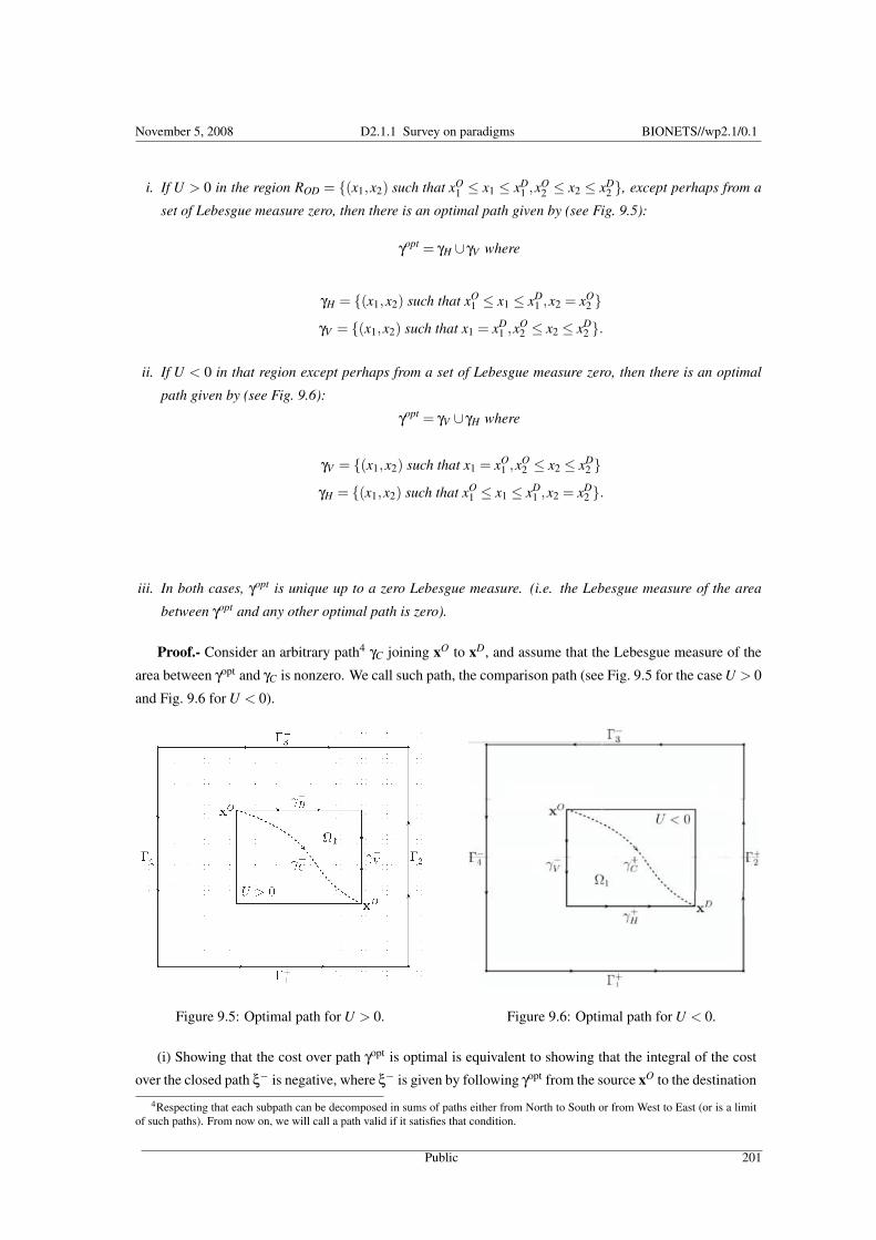
November 5, 2008 D2.1.1 Survey on paradigms BIONETS//wp2.1/0.1
i. If U > 0 in the region ROD = (x1,x2) such that xO1 ≤ x1 ≤ xD
1 ,xO2 ≤ x2 ≤ xD
2 , except perhaps from a
set of Lebesgue measure zero, then there is an optimal path given by (see Fig. 9.5):
γopt = γH ∪ γV where
γH = (x1,x2) such that xO1 ≤ x1 ≤ xD
1 ,x2 = xO2
γV = (x1,x2) such that x1 = xD1 ,xO
2 ≤ x2 ≤ xD2 .
ii. If U < 0 in that region except perhaps from a set of Lebesgue measure zero, then there is an optimal
path given by (see Fig. 9.6):
γopt = γV ∪ γH where
γV = (x1,x2) such that x1 = xO1 ,xO
2 ≤ x2 ≤ xD2
γH = (x1,x2) such that xO1 ≤ x1 ≤ xD
1 ,x2 = xD2 .
iii. In both cases, γopt is unique up to a zero Lebesgue measure. (i.e. the Lebesgue measure of the area
between γopt and any other optimal path is zero).
Proof.- Consider an arbitrary path4 γC joining xO to xD, and assume that the Lebesgue measure of the
area between γopt and γC is nonzero. We call such path, the comparison path (see Fig. 9.5 for the case U > 0
and Fig. 9.6 for U < 0).
Figure 9.5: Optimal path for U > 0. Figure 9.6: Optimal path for U < 0.
(i) Showing that the cost over path γopt is optimal is equivalent to showing that the integral of the cost
over the closed path ξ− is negative, where ξ− is given by following γopt from the source xO to the destination
4Respecting that each subpath can be decomposed in sums of paths either from North to South or from West to East (or is a limitof such paths). From now on, we will call a path valid if it satisfies that condition.
Public 201
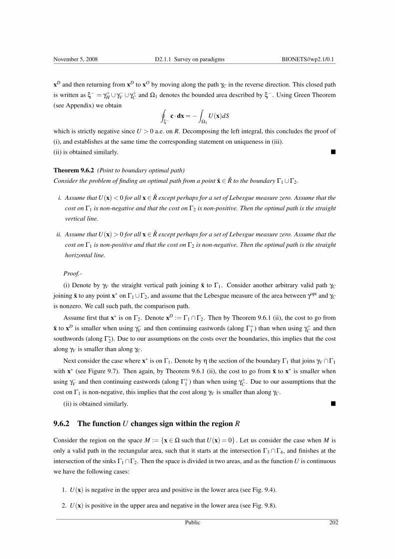
November 5, 2008 D2.1.1 Survey on paradigms BIONETS//wp2.1/0.1
xD and then returning from xD to xO by moving along the path γC in the reverse direction. This closed path
is written as ξ− = γ+H ∪ γ−V ∪ γ+
C and Ω1 denotes the bounded area described by ξ−. Using Green Theorem
(see Appendix) we obtain ∮
ξ−c ·dx =−
∫
Ω1
U(x)dS
which is strictly negative since U > 0 a.e. on R. Decomposing the left integral, this concludes the proof of
(i), and establishes at the same time the corresponding statement on uniqueness in (iii).
(ii) is obtained similarly. ¥
Theorem 9.6.2 (Point to boundary optimal path)
Consider the problem of finding an optimal path from a point x ∈ R to the boundary Γ1∪Γ2.
i. Assume that U(x) < 0 for all x ∈ R except perhaps for a set of Lebesgue measure zero. Assume that the
cost on Γ1 is non-negative and that the cost on Γ2 is non-positive. Then the optimal path is the straight
vertical line.
ii. Assume that U(x) > 0 for all x ∈ R except perhaps for a set of Lebesgue measure zero. Assume that the
cost on Γ1 is non-positive and that the cost on Γ2 is non-negative. Then the optimal path is the straight
horizontal line.
Proof.-
(i) Denote by γV the straight vertical path joining x to Γ1. Consider another arbitrary valid path γC
joining x to any point x∗ on Γ1∪Γ2, and assume that the Lebesgue measure of the area between γopt and γC
is nonzero. We call such path, the comparison path.
Assume first that x∗ is on Γ2. Denote xD := Γ1 ∩Γ2. Then by Theorem 9.6.1 (ii), the cost to go from
x to xD is smaller when using γ−V and then continuing eastwords (along Γ+1 ) than when using γ+
C and then
southwords (along Γ∗2). Due to our assumptions on the costs over the boundaries, this implies that the cost
along γV is smaller than along γC.
Next consider the case where x∗ is on Γ1. Denote by η the section of the boundary Γ1 that joins γV ∩Γ1
with x∗ (see Figure 9.7). Then again, by Theorem 9.6.1 (ii), the cost to go from x to x∗ is smaller when
using γ−V and then continuing eastwords (along Γ+1 ) than when using γ+
C . Due to our assumptions that the
cost on Γ1 is non-negative, this implies that the cost along γV is smaller than along γC.
(ii) is obtained similarly. ¥
9.6.2 The function U changes sign within the region R
Consider the region on the space M := x ∈Ω such that U(x) = 0 . Let us consider the case when M is
only a valid path in the rectangular area, such that it starts at the intersection Γ3 ∩Γ4, and finishes at the
intersection of the sinks Γ1∩Γ2. Then the space is divided in two areas, and as the function U is continuous
we have the following cases:
1. U(x) is negative in the upper area and positive in the lower area (see Fig. 9.4).
2. U(x) is positive in the upper area and negative in the lower area (see Fig. 9.8).
Public 202

November 5, 2008 D2.1.1 Survey on paradigms BIONETS//wp2.1/0.1
η+ ⊆ Γ1
Γ2
Γ3
Γ4
U ≤ 0
γ+
Vγ+
C
1
Figure 9.7: Theorem 9.6.2 (i)
Two other cases where the sign of U is the same over Ω are contained in what we solved in the previous
section (allowing U to be zero on M which has Lebesgue measure zero)
Case 1: The function U(x) is negative in the upper area and positive in the lower area.
We shall show that this case, M is an atractor.
Proposition 9.6.1 Assume that the source x and destination y are both on M. Then the path pM that follows
M is optimal.
Proof.- Consider an alternative path γC that coincides with M only in the source and destination points.
First assume γC is entirely in the upper (i.e. northen) part and call Ω1 the surrounded area. Define ξ+ to be
the closed path that follows pM from x to y and then returns along γC.
The integral∫
Ω1U(x)dS is negative by assumption. By Green Theorem it equals
∮ξ+ c ·dx. This implies
that the cost along pM is strictly smaller than along γC.
A similar argument holds for the case that γC is below pM .
A path between x and y may have several intersections with M. Between each pair of consecutive
intersections of M, the subpath has a cost larger than that obtained by following M between these points
(this follows from the previous steps of the proof). We conclude that pM is indeed optimal. ¥
Proposition 9.6.2 Let a point xO send packets to a point xD.
i. Assume both points in the upper region. Denote by γ1 the two segments path given in Theorem 9.6.1
(ii). Then the curve γ obtained as the maximum between M and γ1 is optimal.5
ii. Let both points be in the lower region. Denote by γ2 the two segments path given in Theorem 9.6.1 (i).
Then the curve γ obtained as the minimum between M and γ2 is optimal.
5By the maximum we mean the following. If γ1 does not intersect M then γ = γ1. If it intersects M then γ agrees with γ1 over thepath segments where γ1 is in the upper region and otherwize agrees with M. The minimum is defined similarly
Public 203

November 5, 2008 D2.1.1 Survey on paradigms BIONETS//wp2.1/0.1
Proof.- (i) A straightforward adaptation of the proof of the previous proposition implies that the path in
the statement of the proposition is optimal among all those restricted to the upper region. Consider now a
path γC that is not restricted to the upper region. Then M∩ γC contains two distinct points such that γC is
strictly lower than M between these points. Applying Proposition 9.6.1 we then see that the cost of γC can
be strictly improved by following M between these points instead of following γC there. This concludes (i).
(ii) is proved similarly. ¥
Proposition 9.6.3 Let a point xO send packets to a point xD.
i. Assume the origin is in the upper region and the destination in the lower one. Then the optimal path
has three segments;
1. It goes straight vertically from xO to M,
2. Continues as long as possible along M, i.e. until it reaches the x coordinate of the destination,
3. At that point it goes straight vertically from M to xD.
ii. Assume the origin is in the lower region and the destination in the upper one. Then the optimal path
has three segments;
1. It goes straight horizontally from xO to M,
2. Continues as long as possible along M, i.e. until it reaches the y coordinate of the destination,
3. At that point it goes straight horizontally from M to xD.
Proof.- The proofs of (i) and of (ii) are the same. Consider an alternative route γC. Let x be some point
in γC ∩M. The proof now follows by applying the previous proposition to obtain first the optimal path
between the origin and x and second, the optimal path between x and the destination. ¥
Case 2: The function U is positive in the upper area and negative in the lower area.
M
Γ1
Γ2
Γ3
Γ4
U > 0
U < 0
1
Figure 9.8: Two regions separated by the curve M. Case 2.
Public 204

November 5, 2008 D2.1.1 Survey on paradigms BIONETS//wp2.1/0.1
This case turns out to be more complex than the previous one. The curve M has some obvious repelling
properties which we state next, but they are not as general as the attractor properties that we had in the
previous case.
Proposition 9.6.4 Assume that both source and destination are in the same region. Then the paths that are
optimal in Theorem 9.6.1 are optimal here as well if we restrict to paths that remain in the same region.
Proof.- Given that the source and destination are in a region we may change the cost over the other
region so that it has the same sign over all the region R. This does not influence the cost of path restricted to
the region of the source-destination pair. With this transformation we are in the scenario of Theorem 9.6.1
which we can then apply. ¥Discussion.- Note that the (sub)optimal policies obtained in Proposition 9.6.4 indeed look like being
repelled from M; their two segments trajectory guarantees to go from the source to the destination as far as
possible from M.
We note that unlike the attracting structure that we obtained in Case 1, one cannot extend the repelling
structure to the case where the paths are allowed to traverse from one region to another.
9.7 User optimization and congestion dependent cost
We go beyond the approach of geometrical optics by allowing the cost to depend on congestion. Shortest
path costs can be a system objective as we shall motivate below. But it can also be the result of decentralized
decision making by many “infinitesimally small" players where a player may represent a single packet (or
a single session) in a context where there is a huge population of packets (or of sessions). The result of
such a decentralized decision making can be expected to satisfy the following properties which define the
so called, user (or Wardrop) equilibrium:
“Under equilibrium conditions traffic arranges itself in congested networks such that all used routes
between OD pair (origin-destination pair), have equal and minimum costs while all unused routes have
greater or equal costs" [30].
Related work.- Both the framework of global optimization as well as the one of minimum cost path
had been studied extensively in the context of road traffic engineering. The use of a continuum network
approach was already introduced on 1952 by Wardrop [30] and by Beckmann [4]. For more recent papers
in this area, see e.g. [6, 7, 14, 16, 32] and references therein. We formulate it below and obtain some of its
properties.
Motivation.- One popular objective in some routing protocols in ad-hoc networks is to assign routes for
packets in a way that each packet follows a minimal cost path (given the others’ paths choices) [11]. This
has the advantage of equalizing source-destination delays of packets that belong to the same class, which
allows one to minimize the amount of packets that come out of sequence. (This is desirable since in data
transfers, out of order packets are misinterpreted to be lost which results not only in retransmissions but
also in drop of systems throughput.)
Traffic assignment that satisfies the above definition is known in the context of road traffic as Wardrop
equilibrium [30].
Public 205

November 5, 2008 D2.1.1 Survey on paradigms BIONETS//wp2.1/0.1
Congestion dependent costWe now add to c1 the dependence on T1 and to c2 the dependence on T2, as in Section 9.4. Let V j(x) be the
minimum cost to go from a point x to B j at equilibrium. Equation (9.12) still holds but this time with ci that
depends on T ji i = 1,2, and on the total flows Ti i = 1,2. Thus (9.13) becomes, ∀ j ∈ 1, . . . ,ν,
0 = mini=1,2
(ci(x,Ti)+
∂V j(x)∂xi
), ∀x ∈ B j ,V j(x) = 0 . (9.14)
We note that if T ji (x) > 0 then by the definition of the equilibrium, i attains the minimum at (9.14). Hence
(9.14) implies the following relations for each traffic class j, and for i = 1,2:
ci(x,Ti)+∂V j
∂xi= 0 if T j
i > 0, (9.15a)
ci(x,Ti)+∂V j
∂xi≥ 0 if T j
i = 0. (9.15b)
This is a set of coupled PDE’s, actually difficult to analyse further.
Beckmann transformationAs Beckmann et al. did in [5] for discrete networks, we transform the minimum cost problem into an
equivalent global minimization one. We shall restrict here to the single class case. To that end, we note that
equations (9.15a)-(9.15b) have exactly the same form as the Kuhn-Tucker conditions (9.6a)-(9.6b), except
that ci(x,Ti) in the former are replaced by ∂g(x,T)/∂Ti(x) in the latter. We therefore introduce a potential
function ψ defined by
ψ(x,T) = ∑i=1,2
∫ Ti
0ci(x,s)ds
so that for both i = 1,2:
ci(x,Ti) =∂ψ(x,T)
∂Ti.
Then the user equilibrium flow is the one obtained from the global optimization problem where we use
ψ(x,T) as local cost. Hence, the Wardrop equilibrium is obtained as the solution of
minT (·)
∫
Ωψ(x,T)dx subject to ∇ ·T(x) = ρ(x), ∀x ∈Ω.
In the special case where costs are given as a power of the flow as defined in eq. (9.7), we observe that
equations (9.15a)-(9.15b) coincide with equations (9.8a)-(9.8b) (up-to a multiplicative constant of the cost).
We conclude that for such costs, the user equilibrium and the global optimization solution coincide.
9.8 Numerical Example
The following example is an adaptation of the road traffic problem solved by Dafermos in [6] to our ad-hoc
setting. We therefore use the notation of [6] for the orientation, as we did in Section 9.4. Thus the direction
from North to South will be our positive x1 axis, and from West to East will be the positive x2 axis. The
framework we study is the user optimization with congestion cost. For each point on the West and/or North
boundary we consider the point to boundary problem. We thus seek a Wardrop equilibrium where each user
can choose its destination among a given set. A flow configuration is a Wardrop equilibrium if under this
Public 206

November 5, 2008 D2.1.1 Survey on paradigms BIONETS//wp2.1/0.1
configuration, each origin chooses a destination and a path to that destination that minimize that users cost
among all its possible choices.
Consider the rectangular area R on the bounded domain Ω defined by the simple closed curve ∂R+ =
Γ+1 ∪Γ+
2 ∪Γ−3 ∪Γ−4 where
Γ1 = 0≤ x1 ≤ a, x2 = 0 , Γ2 = x1 = a, 0≤ x2 ≤ b ,Γ3 = 0≤ x1 ≤ a, x2 = b , Γ4 = x1 = 0, 0≤ x2 ≤ b .
Assume throughout that ρ = 0 for all x ∈ Ω, and that the costs of the routes are linear, i.e.
c1 = k1T1 +h1 and c2 = k2T2 +h2, (9.16)
with k1 > 0, k2 > 0, h1, and h2 constant over Ω.
We are precisely in the framework of section 9.7 and 9.4 with affine costs per packet. As a matter of
fact, the potential function associated with these costs is
ψ(T) =2
∑i=1
∫ Ti
0(kis+hi)ds =
2
∑i=1
(12
kiTi +hi)Ti .
Now, we want to handle a condensation of sources or sinks along the boundary. While this is feasible with
the framework of section 9.4, it is rather technical. We rather use a more direct path below.
Notice that we have in Ω, we have∂T1
∂x1+
∂T2
∂x2= 0.
Take any closed path γ surrounding a region ω. Then by Green formula,
∮
γT1dξ2−T2dξ1 =
∫
ω
∂T1
∂x1+
∂T2
∂x2= 0
Therefore we can define
φ(x) :=∫ x
xoT1dξ2−T2dξ1
the integral will not depend on the path between xo and x and φ is thus well defined, and we have
∂φ(x)∂x2
= T1(x)∂φ(x)∂x1
=−T2(x) . (9.17)
We now make the assumption that there is sufficient demand and that the congestion cost is not too high so
that at equilibrium the traffic T1 and T2 are strictly positive over all Ω [6]. It turns out that all paths to the
destination are used. Thus, from Wardrop’s principle, the cost∫
cdx is equalized between any two paths.
And therefore,∂c1
∂x2=
∂c2
∂x1.
Using the equations in (9.16) then
k1∂T1
∂x2= k2
∂T2
∂x1,
and from equations in (9.17) we have
k1∂2φ∂x2
2+ k2
∂2φ∂x2
1= 0.
Public 207
November 5, 2008 D2.1.1 Survey on paradigms BIONETS//wp2.1/0.1
Let ki = K2i . Divide the above equation by k1k2. One obtains
1K2
1
∂2φ∂x2
1+
1K2
2
∂2φ∂x2
2= 0.
Following the classical way of analyzing the Laplace equation, (see[31]) we attempt a separation of vari-
ables according to
φ(x1,x2) = F1(K1x1)F2(K2x2) .
We then get thatF ′′1 (K1x1)F1(K1x1)
=−F ′′2 (K2x2)F2(K2x2)
= s2 .
In that formula, since the first term in independent on x2 and the second on x1, then both must be constant.
We call s2 that constant, but we do not know its sign. Therefore, s may be imaginary or real. All solutions
of this system for a given s are of the form
F1(x) = Acos(isx)+Bsin(isx) , F2 = C cos(sx)+Dsin(sx) .
As a matter of fact, φ may be the sum of an arbitrary number of such multiplicative decompositions with
different s. We therefore arrive at general formula such as
φ(x1,x2) =∫
[A(s)cos(isK1x1)+B(s)sin(isK1x1)][C(s)cos(sK2x2)+D(s)sin(sK2x2)]ds.
From this formula, we can write T1 and T2 as integrals also. The flow T at the boundaries should be
orthogonal to the boundary, and have the local source density for inward modulus (it is outward at a sink).
There remains to expand these boundary conditions in Fourier integrals to identify the functions A, B, C,
and D. (Surely not a simple matter!) (It is advisable to represent the integrals of the boundary densities
as Fourier integrals, since then the boundary conditions themselves will be of the form s∫
R(s)ds, closely
matching the formulas we obtain for the Ti’s.)
9.9 Conclusions
Routing in ad-hoc networks have received much attention in the massively dense limit. The main tools
to describe the limits had been electrostatics and geometric optics. We exploited another approach for the
problem that has its roots in road traffic theory, and presented both quantitative as well as qualitative results
for various optimization frameworks.
Acknowledgement
We wish to thank Dr. Stavros Toumpis for helpful discussions. The work has been kindly supported by the
Bionets Eurpean Contract.
Public 208
Bibliography
[1] Eitan Altman, Pierre Bernhard and Alonso Silva, "The Mathematics of Routing in Massively Dense Ad-HocNetworks", 7th International Conference on Ad-Hoc Networks and Wireless, September 10 - 12, 2008, SophiaAntipolis, France.
[2] F. Baccelli, B. Blaszczyszyn and P. Muhlethaler, “An ALOHA protocool for multihop mobile wireless networks,”IEEE Transactions on Information Theory, Vol. 52, Issue. 2, 421- 436, Febrary 2006
[3] Martino Bardi and Italo Capuzzo-Dolcetta, Optimal Control and Viscosity Solutions of Hamilton-Jacobi-BellmanEquations, Birkhauser, 1994.
[4] M. Beckmann, “A continuum model of transportation,” Econometrica 20:643-660, 1952.
[5] M. Beckmann, C. B. McGuire and C. B. Winsten, Studies in the Economics and Transportation, Yale Univ. Press,1956.
[6] Stella C. Dafermos, “Continuum Modeling of Transportation Networks,” Transpn Res. Vol. 14B, pp 295–301,1980.
[7] P. Daniele and A. Maugeri, “Variational Inequalities and discrete and continuum models of network equilibriumprotocols,” Mathematical and Computer Modelling 35:689–708, 2002.
[8] Wendell H. Fleming and H. M. Soner, Controlled Markov Processes and Viscosity Solutions. Springer, SecondEdition, 2006.
[9] M. Franceschetti, O. Dousse, D. Tse, P. Thiran, “Closing the gap in the capacity of random wireless networks,” InProc. Inf. Theory Symp. (ISIT), Chicago, IL, July 2004.
[10] M. Grossglauser and D. Tse, “Mobility Increases the Capacity of Ad Hoc Wireless Networks,” IEEE/ACM Trans.on Networking, vol 10, no 4, August 2002.
[11] P. Gupta and P. R. Kumar, “A system and traffic dependent adaptive routing algorithm for ad hoc networks,”Proceedings of the 36th IEEE Conference on Decision and Control, pp. 2375–2380, San Diego, December 1997.
[12] P. Gupta and P. R. Kumar, “The Capacity of Wireless Networks,” IEEE Transactions on Information Theory, vol.IT-46, no. 2, pp. 388–404, March 2000.
[13] G. A. Gupta and S. Toumpis, “Optimal placement of nodes in large sensor networks under a general physical layermodel,” IEEE Secon, Santa Clara, CA, September 2005.
[14] H.W. Ho and S.C. Wong, “A Review of the Two-Dimensional Continuum Modeling Approach to TransportationProblems,” Journal of Transportation Systems Engineering and Information Technology, Vol.6 No.6 P.53–72,2006.
[15] E. Hyytia and J. Virtamo, “On load balancing in a dense wireless multihop network,” Proceeding of the 2ndEuroNGI conference on Next Generation Internet Design and Engineering, Valencia, Spain, April 2006.
[16] G. Idone, “Variational inequalities and applications to a continuum model of transportation network with capacityconstraints,” Journal of Global Optimization 28:45–53, 2004.
[17] P. Jacquet, “Geometry of information propagation in massively dense ad hoc networks,” in MobiHoc ’04: Pro-ceedings of the 5th ACM international symposium on Mobile ad hoc networking and computing, New York, NY,USA, 2004, pp. 157–162, ACM Press.
[18] Jerrold E. Marsden and Anthony J. Tromba, Vector Calculus, Third Edition, W.H. Freeman and Company 1988.
[19] A. MIELE, Extremization of Linear Integrals by Green’s Theorem, Optimization Technics, Edited by G. Leitmann,Academic Press, New york, pp. 69–98, 1962.
209
November 5, 2008 D2.1.1 Survey on paradigms BIONETS//wp2.1/0.1
[20] Venkatesh Ramaiyan, Anurag Kumar, Eitan Altman, “Jointly Optimal Power Control and Hop Length for a SingleCell, Dense, Ad Hoc Wireless Network,” Proc. Modeling and Optimization in Mobile, Ad Hoc and WirelessNetworks, WiOpt, April 2007.
[21] V. Rodoplu and T. H. Meng, “Bits-per-Joule capacity of energy-limited wireless networks,” IEEE Transactionson Wireless Communications, Vol. 6, Number 3, pp. 857-865, March 2007.
[22] I. Stavrakakis R. Ramanathan C. Santinavez, B. McDonald, “On the scalability of ad hoc routing protocols,”IEEE INFOCOM, vol. 3, pp. 1688–1697, 2002.
[23] Alonso Silva, Eitan Altman and Pierre Bernhard, "Numerical solutions of Continuum Equilibria for Routingin Dense Ad-hoc Networks", Workshop on Interdisciplinary Systems Approach in Performance Evaluation andDesign of Computer & Communication Systems (InterPerf), Athens, Greece, October, 2008.
[24] L. Tassiulas and S. Toumpis, “Packetostatics: Deployment of massively dense sensor networks as an electrostaticproblem,” IEEE INFOCOM, vol. 4, pp. 2290–2301, Miami, March 2005.
[25] L. Tassiulas and S. Toumpis, “Optimal deployment of large wireless sensor networks,” IEEE Transactions onInformation Theory, Vol. 52, No. 7, pp 2935-2953, July 2006.
[26] S. Toumpis, “Optimal design and operation of massively dense wireless networks: or how to solve 21st centuryproblems using 19th century mathematics,” in interperf ’06: Proceedings from the 2006 workshop on Interdis-ciplinary systems approach in performance evaluation and design of computer & communications systems, NewYork, NY, USA, 2006, p. 7, ACM Press.
[27] S. Toumpis, “Mother nature knows best: A survey of recent results on wireless networks based on analogies withphysics,” Unpublished.
[28] S. Toumpis, R. Catanuto and G. Morabito, “Optical routing in massively dense networks: Practical issues anddynamic programming interpretation,” Proc. of IEEE ISWCS 2006, September 2006.
[29] T. V. Truong A. Ephremides, “Scheduling broadcasts in multihop radio networks,” IEEE INFOCOM, vol. 38, pp.456–460, 1990.
[30] J.G. Wardrop, “Some theoretical aspects of road traffic research,” Proceedings of the Institution of Civil Engineers,Part II, I:325–378, 1952.
[31] H. Weinberger, A First Course in Partial Differential Equations with Complex and Transform Methods, DoverBooks on Mathematics.
[32] S.C.Wong, Y.C.Du, J.J.Sun and B.P.Y.Loo, “Sensitivity analysis for a continuum traffic equilibrium problem,”Ann Reg Sci 40:493–514„ 2006.
9.10 Appendix: Mathematical ToolsTheorem 9.10.1 (Green’s Theorem) Let Ω ⊆ X be a region of the space, and let Γ be its boundary. Suppose thatP,Q∈ C 1(Ω) (We denote C 1(Ω) the set of functions that are differentiable and whose partial derivatives are continuouson Ω.) Then ∮
Γ+Pdx+Qdy =
∫
Ω
(∂Q∂x− ∂P
∂y
)dxdy. (9.18)
Public 210

Part III
Socio-Economic Paradigms
211


Chapter 10
Historical-Interpretive Considerationsabout Money as a Unit of Value andScale-Dependent PhenomenonS. Elaluf-Calderwood
10.1 IntroductionThis document aims to present a sectional overview of the social, economic and technological aspects that need tobe taken into account when understanding the potential application for the Economics of Sharing and/or CommunityCurrencies socio-economic models in the BIONETS environment. These models have been actively used over timebut since economic interconnections tend to be of a socio-geographical nature (Schraven, 2001), the adoption of suchmodels has been highly ideologically motivated, such as in the case of the Local Exchange and Trading Systems (LETS)(Cadwell, 2000). Membership of these types of economic initiatives has been exclusive of the average population andnot economically motivated, and is sustained by considerable social effort in the medium and long term (Schraven,2001). A similar situation occurs in the case of complementary currencies, which can coexist with national currencies.
The rise of mobile technology and the multiple applications and services that can be provided directly to users offersthe opportunity to liberate the economics of sharing and community currencies from the ideological trap, allowing theirusers to create a wider user base where exchanges are economically motivated. Ubiquitous technology such as mobiledevices raises new possible applications in a virtual world for how to understand, apply and negotiate these concepts.This is a new area of social interaction being researched by social scientists. If technology increases the ability ofpeople to share, the question still pending is whether they will share more than just those goods and services that canbe exchanged by means of technology? (The Economist, 2005).
This paper is structured in five sections. The first section discusses a global abstraction of the common idea ofmoney as a phenomenon that is historically interpretative. The second and third sections reflect upon the meaningand ideological abstractions linked to the concepts of community currencies and the economics of sharing. The fourthsection covers a further in-depth analysis of mobile technology as a potential new economic agent-mediator as well assome business examples of how mobile users, and in general IT users, are using technology to establish new socio-economic money trade-offs. Finally, some words about further research in the area using the BIONETS infrastructureat the application layer ends this paper.
10.2 Historical BackgroundMoney has a social interpretive value and this is clear if seeking a definition of money using neo-classical economics.In the Economics field there are several definitions of money; some of these definitions overlap others and othershave distinct semantic boundaries. In this document the discussion of money is limited to the meaning it has acquiredthrough a consensual process, highlighting the social interpretation of the idea of money over other categorizations.Thus, money is commonly defined by the functions attached to any good or token that functions in trade as a medium
213

November 5, 2008 D2.1.1 Survey on paradigms BIONETS//wp2.1/0.1
of exchange, store of value, and unit of account (Wikipedia, 2006). In everyday use money refers more specifically tocurrency, and the circulation of currencies with a legal tender status, which works as a standard of deferred payment.Historically commodity money systems were the first to appear; exchanges in salt, iron, copper, gold, silver, preciouswoods, etc. were used for trade, firstly between individuals, then social groups, and finally communities, tribes ornations. A main characteristic of commodity money is the fact that, in addition to the value the money mediates, thereis an intrinsic value to the currency being traded; for example, wood can be used to build buildings besides being traded.This type of money value differs from the barter model in which goods are given equal value for trade; or even from thesocially-based, multiple-commodity currency used by medieval towns in the Hanseatic league in the Northern areas ofEurope (Menger, 1982).
Modern barter models deserve a more in-depth analysis in light of the fact that it has been used as the referencemodel of choice by modern community currencies such as LETS. The barter model encourages people to exchangegoods and services within their local communities, creating an alternative economy outside, and parallel to, the widereconomy, to which the community might belong to. The barter economy was highly developed during Medieval timesfor practical reasons: the lack of readily available gold currency for trade made this model a common practice, since itrelies on reciprocity, distribution and trust for its sustainability.
Figure 1 is an illustration of a medieval Sunday Village Fair. All members of the village joined the common area andexchanged goods, news and other items. It is known that visitor traders from outside the village would have presentedsome form of accreditation to the local authorities, before proceeding to trade. The European Medieval village is a richsource of metaphors for community currencies and economics of sharing. The barter model would have been the choicebetween the members of the community as it would have coexisted in parallel with currency brought to the communityby visitor traders.
Figure 10.1: The Medieval Village: Barter economy and multiple community currencies in action
In the Medieval Village there is limited centralization when issuing money or currency. There is trust betweenvillagers or group of villagers at trading time for goods or services. The shift in money priorities between the feudaland capitalist systems can be seen from the contrasting modern description of money. Based on common understandingof the phenomenon, this is commonly identified with ÒFiat MoneyÓ, in which a central authority such as a nationalgovernment creates a new money object that has negligible inherent value. The widespread acceptance of Fiat Moneyis most frequent when the central authority mandates the acceptance of money under penalty of law and demands thismoney in payment of taxes or tribute.
According to this centralized view, money needs to be provided with some essential value characteristics. The
Public 214
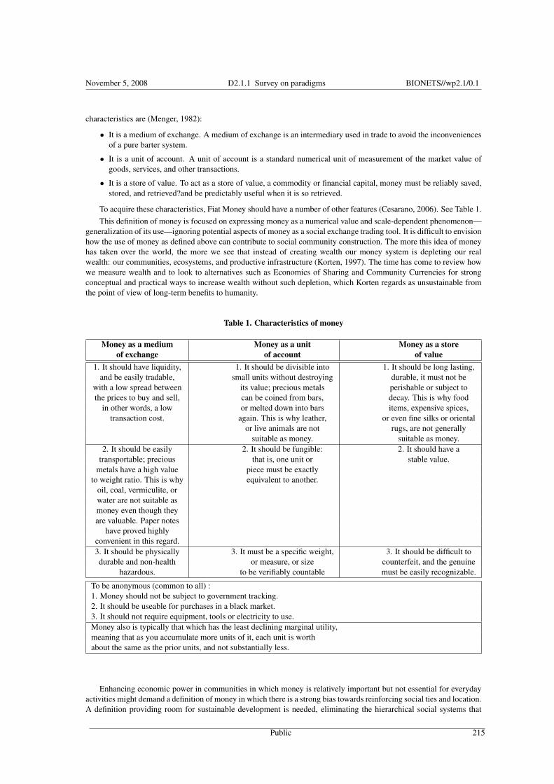
November 5, 2008 D2.1.1 Survey on paradigms BIONETS//wp2.1/0.1
characteristics are (Menger, 1982):
• It is a medium of exchange. A medium of exchange is an intermediary used in trade to avoid the inconveniencesof a pure barter system.
• It is a unit of account. A unit of account is a standard numerical unit of measurement of the market value ofgoods, services, and other transactions.
• It is a store of value. To act as a store of value, a commodity or financial capital, money must be reliably saved,stored, and retrieved?and be predictably useful when it is so retrieved.
To acquire these characteristics, Fiat Money should have a number of other features (Cesarano, 2006). See Table 1.This definition of money is focused on expressing money as a numerical value and scale-dependent phenomenon—
generalization of its use—ignoring potential aspects of money as a social exchange trading tool. It is difficult to envisionhow the use of money as defined above can contribute to social community construction. The more this idea of moneyhas taken over the world, the more we see that instead of creating wealth our money system is depleting our realwealth: our communities, ecosystems, and productive infrastructure (Korten, 1997). The time has come to review howwe measure wealth and to look to alternatives such as Economics of Sharing and Community Currencies for strongconceptual and practical ways to increase wealth without such depletion, which Korten regards as unsustainable fromthe point of view of long-term benefits to humanity.
Table 1. Characteristics of money
Money as a medium Money as a unit Money as a storeof exchange of account of value
1. It should have liquidity, 1. It should be divisible into 1. It should be long lasting,and be easily tradable, small units without destroying durable, it must not be
with a low spread between its value; precious metals perishable or subject tothe prices to buy and sell, can be coined from bars, decay. This is why food
in other words, a low or melted down into bars items, expensive spices,transaction cost. again. This is why leather, or even fine silks or oriental
or live animals are not rugs, are not generallysuitable as money. suitable as money.
2. It should be easily 2. It should be fungible: 2. It should have atransportable; precious that is, one unit or stable value.
metals have a high value piece must be exactlyto weight ratio. This is why equivalent to another.
oil, coal, vermiculite, orwater are not suitable asmoney even though theyare valuable. Paper notes
have proved highlyconvenient in this regard.3. It should be physically 3. It must be a specific weight, 3. It should be difficult todurable and non-health or measure, or size counterfeit, and the genuine
hazardous. to be verifiably countable must be easily recognizable.
To be anonymous (common to all) :1. Money should not be subject to government tracking.2. It should be useable for purchases in a black market.3. It should not require equipment, tools or electricity to use.Money also is typically that which has the least declining marginal utility,meaning that as you accumulate more units of it, each unit is worthabout the same as the prior units, and not substantially less.
Enhancing economic power in communities in which money is relatively important but not essential for everydayactivities might demand a definition of money in which there is a strong bias towards reinforcing social ties and location.A definition providing room for sustainable development is needed, eliminating the hierarchical social systems that
Public 215

November 5, 2008 D2.1.1 Survey on paradigms BIONETS//wp2.1/0.1
are the product of centrally controlled money, since in most cases this type of money has drawbacks when socialcommunities need to be built and sustained over time. For this type of money to be sustainable, social participation needsto be committed to developing trust between both individuals and social groups, extending to nations or geographicaldistributed governments. If the idea of modern mutual banking was proposed only in the 19th century (by Frenchsocial-anarchist Proudhom (Wikipedia, 2006) ), it is possible to see that, compared to human trade, this type of moneyhas existed over a historically short time span, and changes in attitude to money and shifts in social practices in thenear future cannot be ruled out. Such an approach can create a shift in our understanding of money as a meta-modelmonopolizing control over the issue of value and currency.
These ideas are not new; in the early 20th Century Silvio Gesell—the founder of the school of Free Economics—envisaged money liberated from interest (Gesell, 1929). The gain of interest for money is one of the major preoccupa-tions linked to the use of money, in fact the demand for interest historically strengthened the concentration of money inthe hands of the rich as a way of further financing the expansion of national economies, imposing demands on futureeconomic resources. Gesell disputed this idea. In his eyes money was in fact a service to the community to the users(Van Arkel and Peterse, 1998). He proposed that everyone having money in their hands at a certain point of time shouldpay a liquidity tax on the possession of money; in his view this tax would make people want to lose the money as soonas possible. They would buy something for it, invest it in durable goods or lend it, so that money had its unlimitedexchange function again, without the need to offer the moneyÕs owner profit on lending. Gessell thought that thispractice would liberate the economic system from the grip of interest. In our times with computer technology this ideais feasible. Lietaer, who coordinated from Brussels the introduction of the European Monetary Union (EMU), followsGesells; in some way he is also seeking to use money without the liability of interest; in other ways, there is renewedsearch for a system in which people are stimulated to spend their money directly and at the same time to take care ofthe future (Van Arkel and Peterse, 1998).
LietaerÕs view reduces the functions of money to two: money as a measuring unit and money as a unit of exchangethat can be abstracted further by trading money via electronic systems for money. Already in Stock Exchanges all overthe world, gold and paper money can be traded electronically via online systems. It is speculated that in the near futuredeveloped economies may migrate from the present system of physical money to an entirely digital currency system.As stated in the title of this paper, money is becoming a form of social information, hence the need to re-evaluate whatmoney is, and its real contribution to the management of material and human resources available now and in future.
The vision of Gesells and Lietaer can be easily implemented with modern real-time computer technology as themoney functions for storing and exchanging are merged into one. Money circulates faster and faster as electronicsystems are in place, hence money owners either circulate it or lend it. Because of this it is possible to stimulate aneconomy without the involvement of interest. Once interest is not required, the idea of money tenure has changed.The idea of future income will be directed to consuming products with a longer life span, which might be perceivedas reducing the stimulus for economic growth, but from another perspective it can also be seen as encouraging thedevelopment of a more durable and stable economy. These types of thoughts are basic assumptions in the models thatwill be explained in sections two and three, in which sustainability is at the core of the socio-economical models to bepresented.
We should clarify that the economics of sharing discussed in this paper as one of the phenomena underpinningcommunity currencies are mainly focussed on sharing unused capital and do not include the open source phenomenonor the processes and interactions collectively referred to as the Gift Economy.
10.3 Community currencies working framework
Besides the shift in the ideas about money presented above—requiring stronger community participation in the useof money—community currencies can be explained in parallel to the historical evolution of the idea of ÒCommonsÓas a means for structuring rights to access, use and control over resources (Benkler, 2006). Working commons needto define in the first instance their accessibility, either as restricted to members or open to all; in the second instancecommons need to define whether their workable system is regulated or unregulated. Depending on which combinationof these two parameter definitions is workable, four types of commons can be classified. See table 2.1 below.
Table 2. Commons as a unit of cohesion for Community Currencies(Sourced from description by Benkler (2006))
Public 216
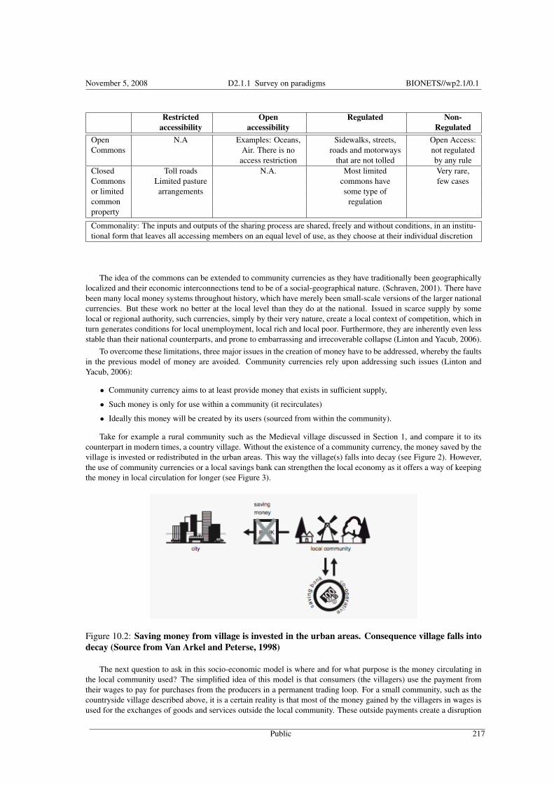
November 5, 2008 D2.1.1 Survey on paradigms BIONETS//wp2.1/0.1
Restricted Open Regulated Non-accessibility accessibility Regulated
Open N.A Examples: Oceans, Sidewalks, streets, Open Access:Commons Air. There is no roads and motorways not regulated
access restriction that are not tolled by any ruleClosed Toll roads N.A. Most limited Very rare,Commons Limited pasture commons have few casesor limited arrangements some type ofcommon regulationproperty
Commonality: The inputs and outputs of the sharing process are shared, freely and without conditions, in an institu-tional form that leaves all accessing members on an equal level of use, as they choose at their individual discretion
The idea of the commons can be extended to community currencies as they have traditionally been geographicallylocalized and their economic interconnections tend to be of a social-geographical nature. (Schraven, 2001). There havebeen many local money systems throughout history, which have merely been small-scale versions of the larger nationalcurrencies. But these work no better at the local level than they do at the national. Issued in scarce supply by somelocal or regional authority, such currencies, simply by their very nature, create a local context of competition, which inturn generates conditions for local unemployment, local rich and local poor. Furthermore, they are inherently even lessstable than their national counterparts, and prone to embarrassing and irrecoverable collapse (Linton and Yacub, 2006).
To overcome these limitations, three major issues in the creation of money have to be addressed, whereby the faultsin the previous model of money are avoided. Community currencies rely upon addressing such issues (Linton andYacub, 2006):
• Community currency aims to at least provide money that exists in sufficient supply,
• Such money is only for use within a community (it recirculates)
• Ideally this money will be created by its users (sourced from within the community).
Take for example a rural community such as the Medieval village discussed in Section 1, and compare it to itscounterpart in modern times, a country village. Without the existence of a community currency, the money saved by thevillage is invested or redistributed in the urban areas. This way the village(s) falls into decay (see Figure 2). However,the use of community currencies or a local savings bank can strengthen the local economy as it offers a way of keepingthe money in local circulation for longer (see Figure 3).
Figure 10.2: Saving money from village is invested in the urban areas. Consequence village falls intodecay (Source from Van Arkel and Peterse, 1998)
The next question to ask in this socio-economic model is where and for what purpose is the money circulating inthe local community used? The simplified idea of this model is that consumers (the villagers) use the payment fromtheir wages to pay for purchases from the producers in a permanent trading loop. For a small community, such as thecountryside village described above, it is a certain reality is that most of the money gained by the villagers in wages isused for the exchanges of goods and services outside the local community. These outside payments create a disruption
Public 217
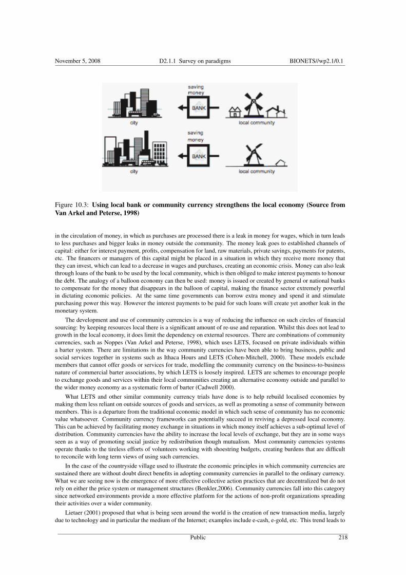
November 5, 2008 D2.1.1 Survey on paradigms BIONETS//wp2.1/0.1
Figure 10.3: Using local bank or community currency strengthens the local economy (Source fromVan Arkel and Peterse, 1998)
in the circulation of money, in which as purchases are processed there is a leak in money for wages, which in turn leadsto less purchases and bigger leaks in money outside the community. The money leak goes to established channels ofcapital: either for interest payment, profits, compensation for land, raw materials, private savings, payments for patents,etc. The financers or managers of this capital might be placed in a situation in which they receive more money thatthey can invest, which can lead to a decrease in wages and purchases, creating an economic crisis. Money can also leakthrough loans of the bank to be used by the local community, which is then obliged to make interest payments to honourthe debt. The analogy of a balloon economy can then be used: money is issued or created by general or national banksto compensate for the money that disappears in the balloon of capital, making the finance sector extremely powerfulin dictating economic policies. At the same time governments can borrow extra money and spend it and stimulatepurchasing power this way. However the interest payments to be paid for such loans will create yet another leak in themonetary system.
The development and use of community currencies is a way of reducing the influence on such circles of financialsourcing: by keeping resources local there is a significant amount of re-use and reparation. Whilst this does not lead togrowth in the local economy, it does limit the dependency on external resources. There are combinations of communitycurrencies, such as Noppes (Van Arkel and Peterse, 1998), which uses LETS, focused on private individuals withina barter system. There are limitations in the way community currencies have been able to bring business, public andsocial services together in systems such as Ithaca Hours and LETS (Cohen-Mitchell, 2000). These models excludemembers that cannot offer goods or services for trade, modelling the community currency on the business-to-businessnature of commercial barter associations, by which LETS is loosely inspired. LETS are schemes to encourage peopleto exchange goods and services within their local communities creating an alternative economy outside and parallel tothe wider money economy as a systematic form of barter (Cadwell 2000).
What LETS and other similar community currency trials have done is to help rebuild localised economies bymaking them less reliant on outside sources of goods and services, as well as promoting a sense of community betweenmembers. This is a departure from the traditional economic model in which such sense of community has no economicvalue whatsoever. Community currency frameworks can potentially succeed in reviving a depressed local economy.This can be achieved by facilitating money exchange in situations in which money itself achieves a sub-optimal level ofdistribution. Community currencies have the ability to increase the local levels of exchange, but they are in some waysseen as a way of promoting social justice by redistribution though mutualism. Most community currencies systemsoperate thanks to the tireless efforts of volunteers working with shoestring budgets, creating burdens that are difficultto reconcile with long term views of using such currencies.
In the case of the countryside village used to illustrate the economic principles in which community currencies aresustained there are without doubt direct benefits in adopting community currencies in parallel to the ordinary currency.What we are seeing now is the emergence of more effective collective action practices that are decentralized but do notrely on either the price system or management structures (Benkler,2006). Community currencies fall into this categorysince networked environments provide a more effective platform for the actions of non-profit organizations spreadingtheir activities over a wider community.
Lietaer (2001) proposed that what is being seen around the world is the creation of new transaction media, largelydue to technology and in particular the medium of the Internet; examples include e-cash, e-gold, etc. This trend leads to
Public 218

November 5, 2008 D2.1.1 Survey on paradigms BIONETS//wp2.1/0.1
trade utilizing multiple currencies: local, national and international. There is no need to choose one currency over theother as they could all coexist, closing a circle of economic models that have been tried since Medieval times. It seemsthat in order to establish trust within the community members, the formation of closed commons in which there areregulated norms for trading and membership are more successful than open commons in which anyone can participate.This seems to be the case for most online communities that have embarked on these types of schemes. The discussionthen has to reflect upon the motivations for trading or sharing that lead to the search for such economic models, as willbe presented in the section below.
10.4 Economics of sharing
Most of the contemporary economic models adopt a very simple model for human motivation: the basic assumptionis that all human motivations can be more or less reduced to positive or negative utilities—things people want, andthings people want to avoid. These utilities are all represented by the money or currency exchange by the societymembers. There is plenty of room to discuss these assumptions, which are obviously not always correct in representingthe diverse social frameworks in which humans operate. The continuous presence of community currencies in socialhistory has shown that humans do have other motivations besides the accumulation of money for their consumptionof utilities, especially if there is a long-term view of how to use and manage human and natural resources. Like anyother economic theory dominant in the 20th Century, the utility assumption is currently subject to a revisionist process,where economic models can widen their assumptions for human motivation by creating a distinction between intrinsicand extrinsic motivations.
Extrinsic motivations are imposed on humans by external factors, and social pressure then reduces the room forintrinsic motivations. There are two rewards associated with human beings in a social structure: economic and socialstanding (Granovetter, 2000). As technological developments make society better networked, new ways of socialproduction emerge (Castells, 1996). Even so, post-modern sharing is emerging from certain physical, rivalrous goodsand will increase due to advances in technology (Benkler,2006). Until now this sharing has not been extended to thespheres of social sharing, in which a third mode of organizing economic production, alongside markets and the state(Benkler, 2004) is being built up.
Intrinsic motivations such as the need for belonging to a community and being valued not only by the products orgoods consumed, but also through the exchange of money, are better expressed in this post-modern sharing of resources.The economics of sharing is departing from these models of human motivation, searching for a motivation for humaneconomic activity that goes beyond the value of human actions based on money exchanges, building upon human capitalto create a more optimal distribution of wealth and resources that give not only a material but also a spiritual reward.What is understood as sharing is the ability to motivate human interaction or sociality besides the need to be awardedmoney for exchanging goods and services. The source of this type of sharing is a way of providing an interpretive andsubjective space in which humans can allocate a subjective value to the sharing.
Current economics of sharing models contextually attached to the use of mobile technology are evolving overservices platforms that are social networks in digital forms; the driver to share is expressed in several modes, forexample:
• Sharing and distribution of electronic tokens between social networks of friends using I-mode enabled phonesin Japan (Rheingold, 2002)
• Sharing tokens, or paying for services through mobile services that are centralized, such as car parks, vendingmachines, and others.
• Sharing Contribution to the fitness valuation of mobile services, sharing moods or opinions about service quality.
• Bluetooth/Wifi sharing of information in digital format (MP3s)
• Video Sharing (www.mytube.com), now on mobile format
These are basic forms of sharing that have been adopted by many mobile users around the world; a valid questionwill be to ask how a sustainable economic model of sharing, developed through mobile services, can be defined. Untilnow, sharing has provided only limited exchange between small groups of friends (e.g. Java applets) but has not linkedsuch exchange to any monetary value. It is possible however to forecast a near future in which the economics of sharingwill develop to produce exchanges in which the interest shown by the community of users would account for a variableexchange value for the goods or services exchanged.
Public 219
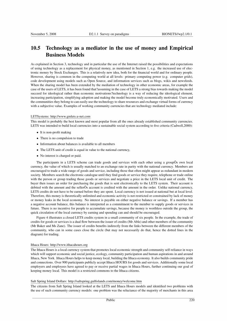
November 5, 2008 D2.1.1 Survey on paradigms BIONETS//wp2.1/0.1
10.5 Technology as a mediator in the use of money and EmpiricalBusiness Models
As explained in Section 3, technology and in particular the use of the Internet raised the possibilities and expectationsof using technology as a replacement for physical money, as mentioned in Section 1, e.g. the increased use of elec-tronic money by Stock Exchanges. This is a relatively new idea, both for the financial world and for ordinary people.However, sharing is common in the computing world at all levels: primary computing power (e.g. computer grids),code development using models such as Open Source, and information services such as blogs, wikis and newsfeeds.When the sharing model has been extended by the mediation of technology in other economic areas, for example thecase of the users of LETS, it has been found that?assuming in the case of LETS a strong bias towards making the modelsucceed for ideological rather than economic motivations?technology is a way of reducing the ideological element,increasing participation, simplifying adoption and making the model become truly economically motivated. Users andthe communities they belong to can easily use the technology to share resources and exchange virtual forms of currencywith a subjective value. Examples of working community currencies that are technology mediated include:
LETSystems: http://www.gmlets.u-net.comThis model is probably the best known and most popular from all the ones already established community currencies.LETS was intended to build local currencies into a sustainable social system according to five criteria (Cadwell,2000):
• It is non-profit making
• There is no compulsion to trade
• Information about balances is available to all members
• The LETS unit of credit is equal in value to the national currency,
• No interest is charged or paid.
The participants in a LETS scheme can trade goods and services with each other using a groupÕs own localcurrency, the value of which is usually matched to an exchange rate in parity with the national currency. Members areencouraged to trade a wide range of goods and service, including those that often might appear as redundant in modernsociety. Members search the electronic catalogue until they find goods or service they require, telephone or trade onlinewith the person or group trading those goods or services and negotiate a price in the LETS local unit of credit. Thebuyer then issues an order for purchasing the goods that is sent electronically to the LETS system. Their account isdebited with the amount and the sellerÕs account is credited with the amount in the order. Unlike national currency,LETS credits do not have to be earned before they are spent. Local currency is not issued at national but at local level.Therefore, this money is theoretically unlimited and economic activity is not restricted or constrained by lack of moneyor money leaks in the local economy. No interest is payable on either negative balance or savings. If a member hasa negative account balance, this balance is interpreted as a commitment to the member to supply goods or services infuture. There is no incentive for people to accumulate savings, because the money is worthless outside the group, thequick circulation of the local currency by earning and spending can and should be encouraged.
Figure 4 illustrates a closed LETS credits system in a small community of six people. In the example, the trade ofcredits for goods or services is a dual flow between the issuer of credits (Mr Able) and other members of the community(Mr Baker and Ms Zane). The issuer of credits benefits indirectly from the links between the different members of thecommunity, who can in some cases close the circle (but may not necessarily do that, hence the dotted lines in thediagram) for trading.
Ithaca Hours: http://www.ithacahours.orgThe Ithaca Hours is a local currency system that promotes local economic strength and community self-reliance in wayswhich will support economic and social justice, ecology, community participation and human aspirations in and aroundIthaca, New York. Ithaca Hours helps to keep money local, building the Ithaca economy. It also builds community prideand connections. Over 900 participants publicly accept Ithaca HOURS for goods and services. Additionally some localemployers and employees have agreed to pay or receive partial wages in Ithaca Hours, further continuing our goal ofkeeping money local. This model is a restricted commons to the Ithaca citizens.
Salt Spring Island Dollars: http://saltspring.gulfislands.com/money/welcome.htmThe citizens from Salt Spring Island looked at the LETS and Ithaca Hours models and identified two problems withthe use of such community currency models: one problem was the reluctance of the majority of merchants in this area
Public 220

November 5, 2008 D2.1.1 Survey on paradigms BIONETS//wp2.1/0.1
to accept such currency unless the currency was 100% redeemable into their national currency; the second problemwas how and when the currency was in circulation to receive and/or maintain any value for the holder. In addition theoperation of local currencies was segregated from local financial institutions. The way these problems were addressedwas to give the currency a two year expiry date; any bills not redeemed by the expiry date would represent a profit. Bycreating a profit concept, to cover costs, it made it possible for the currency to go into circulation through a one-to-oneexchange with the Canadian Dollar. The system went live in 2001. Given that the island has a population of around10,000 with an annual tourist flow of over 200,000, a potential edition of 20,000 has a considerable base. The currencyis now issuing coins made of precious metals and complies with all the aims and goals that other community currencieshave established.
Figure 10.4: An illustration model of how the LETS credits can be used within a local community
Strohalm: http://www.strohalm.org/vlcs.htmlThe Social Trade Organisation, STRO (in Dutch STROhalm), is a Research & Development network working in
the field of micro-credit, development of small and medium enterprises and strengthening of local economies throughcomplementary circuits of exchange. The basic tool of the methodologies of STRO is a circuit of exchange betweenproducers and consumers. A part of the flow of money that enters a community through the purchasing power of theseconsumers, or connected governmental agencies, is circulating several times through the exchange circuit before itleaves the area, to bring as much unused capacities as possible back into productivity. Some of their projects are fo-cussing on the very first step towards entrepreneurship, whilst others are more elaborated tools to optimise the outreachof the existing economic actors. All projects aim to result in more employment, income and opportunities for localcommunities to improve their living conditions. Most of the pilot-projects are concentrated in Brazil, Central-America,Asia and the Netherlands.
Brazilian Educational Currency (Saber): See Lietaer (2006b).The main learning focus of this currency is to multiply the number of students that can afford to obtain a college-
level education in Brazil. The approach is to create a special targeted currency, whose unit is called Saber, whichwould be issued under highly controlled conditions in the educational system. Its face value would be nominally thesame as a Reai (Brazilian currency), and would be redeemable for tuition in higher education programs in participatinguniversities. This would be a paper currency (although electronic accounts can be kept where they will accumulate),
Public 221
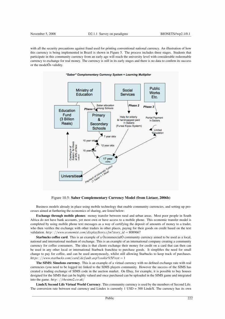
November 5, 2008 D2.1.1 Survey on paradigms BIONETS//wp2.1/0.1
with all the security precautions against fraud used for printing conventional national currency. An illustration of howthis currency is being implemented in Brazil is shown in Figure 5. The process includes three stages. Students thatparticipate in this community currency from an early age will reach the university level with considerable redeemablecurrency to exchange for real money. The currency is still in its early stages and there is no data to confirm its successor the modelÕs validity.
Figure 10.5: Saber Complementary Currency Model (from Lietaer, 2006b)
Business models already in place using mobile technology that enable community currencies, and setting up pro-cesses aimed at furthering the economics of sharing, are listed below:
Exchange through mobile phones: money transfer between rural and urban areas. Most poor people in SouthAfrica do not have bank accounts, yet most own or have access to a mobile phone. This economic transfer model iscompleted by using mobile phone text messages as a way of certifying the deposit of amounts of money to a trader,who then verifies the exchange with other traders in other places, paying for their goods on credit based on the textvalidation. htt p : //www.economist.com/displayStory.c f m?story_id = 8089667
Starbucks coffee card. This is an example of a ÒcommercialÓ community currency aimed to be used as a local,national and international medium of exchange. This is an example of an international company creating a communitycurrency for coffee consumers. The idea is that clients exchange their money for credit on a card that can then canbe used in any other local or international Starbuck franchise to purchase goods. It simplifies the need for smallchange to pay for coffee, and can be used anonymously, whilst still allowing Starbucks to keep track of purchases.htt ps : //www.starbucks.com/card/de f ault.asp?cookie%5Ftest = 1
The SIMS: Simelons currency. This is an example of a virtual currency with no defined exchange rate with realcurrencies (you need to be logged in) linked to the SIMS players community. However the success of the SIMS hascreated a trading exchange of SIMS code in the auction market. On Ebay, for example, it is possible to buy housesdesigned for the SIMS that can be highly valued and once purchased can be uploaded in the SIMS game and integratedinto the game. htt p : //thesims2.co.uk/
LindeX Second Life Virtual World Currency. This community currency is used by the members of Second Life.The conversion rate between real currency and Lindex is currently 1 USD = 300 LindeX. The currency has its own
Public 222

November 5, 2008 D2.1.1 Survey on paradigms BIONETS//wp2.1/0.1
stock market, and it is used to purchase all types of goods and services in the virtual community; it is a closed common,and extremely popular. htt p : //secondli f e.com/whatis/currency.php
My gamma. This community currency does not exchange money as such but knowledge, social networks, friend-ships and other tokens. It is particularly popular in Asia (now extending its influence to Europe and Africa). The tradingis also token based and the value assigned to some of those tokens is subjective and depends upon the demand for them.Exchange rates are variable and determined by the supply-demand relationships. (See htt p : //www20.mygamma.com/rankdisplay.php?country =uk&i = 1 or htt p : //en.wikipedia.org/wiki/MyGamma)
The models listed above are based on sharing common resources provided by technological development based onthe theoretical socio-economical models; there are however additional characteristics of note:
• The sharing is free from geographical restrictions
• When there is a virtual or real currency to be traded, the value assigned to the unit is universally accepted by allpartners.
• There is a conversion exchange rate between the virtual and the real world.
In real terms the mediation of technology allows the easy creation, accountability, and trade of virtual currencies,some of them follow the conventional idea of money discussed in Section 1 of this paper, whilst others have followedthe path established by community currencies. However it is clear that this trend in associating parallel currencieswith national currencies will continue and become more sophisticated as technology advances further, perhaps makingincursions into areas of trade currently based on conventional models. Nascent technologies which might further thistrend include exchanges of identity and DNA samples. It is important to understand that the creation and measurementof wealth will have to be reconceptualized to include the new exchange opportunities opened to all people through thetechnology.
10.6 Further research applied to BIONETSThis document has presented an overview of how money as a concept has changed over time as well as a compendiumof knowledge about social economic models for Economics of Sharing and Community Currencies. The relevance ofsuch concepts applied to the BIONETS service creation development model can be seen as self-evolving, autonomic,aimed at gaining the best support for user tasks while reducing the efforts of the user in service creation. From this pointof view, there exist opportunities to research scenarios where the technology is used selectively, both by individuals andby the social networks linked by the distributed applications available from BIONETS services. There are alreadyindicators that such platforms will lead to an exchange of services and goods beyond those based on the technology.
For example, researchers at Nokia speculate that, within a decade, the cost of storage will have fallen so far that itmight be possible to store every piece of music ever recorded on a single chip that could be included in each phone.It would be necessary to update the chip every so often to allow for new releases, of course. But this could open upnew business models that do not depend on downloading music over the airwaves; instead, the phone could simplyexchange brief messages with a central server to unlock purchased tracks or report back on what the user had listenedto for billing purposes (The Economist, 2006). This type of exchange will raise the opportunity to create communitiesin which music recording might be the currency of trade associated with that community.
There is also the possibility of using mobile phone applications to confirm transactions with one another by simplypressing a button. A central or distributed server could confirm that a transaction has been completed. This will besimilar to enabling the back-end for a truly decentralized marketplace with buyers, sellers, traders, and sharers in anOpen Source killer application for the 21st Century (Rushkoff, 2004)
In terms of the BIONETS service layer as the project advances and applications are developed using the BIONETSinfrastructure, it will be possible to put to test some of the concepts discussed in this document. Special mentioncan be given to the planned undersound (Bassoli, 2006) experience where there is the opportunity to create a tokentrade community currency based on music. The core of research and development currently being undertaken bycomputing and science researchers in the project points towards a significant benefit of the BIONETS architecturedesign compared with traditional or currently available mobile networks. For example, the T-Node/U-Node separation,evolving applications, inherent user feedback, etc. might represent a wider technology platform providing more—andÒbuilt-inÓ—support for sharing and community currencies. At this stage of the project these are promising avenuesfor deploying and exploring such models that require further research.
As an introduction to the concepts in the area of money, community currencies, and economics of sharing, thispaper has aimed to link these ideas to applications and services already available, as well as to explore some of thebenefits and drawbacks of such uses.
Public 223

November 5, 2008 D2.1.1 Survey on paradigms BIONETS//wp2.1/0.1
10.7 ReferencesBassoli, A (2006). Òundersound: exploring the experience of riding the UndergroundÓ. London, UK, Media and
Communications Department, The London School of Economics and Political Science: 37.Benkler, Y (2004). ÒSharing Nicely: On Shareable Goods and the Emergence of Sharing as a Modality of Economic
ProductionÓ. Yale Law Journal. Available athtt p : //www.yalelaw journal.org/pd f /114−2/BenklerF INALY LJ114−2.pd f
Benkler, Y (2006). The Wealth of Networks: How Social Production Transforms Markets and Freedom. New Havenand London, Yale University Press.
BIONETS (2006). BIONETS Service Life-Cycle. Internal Report, BIONETS.Castells, M (1996). The Rise of the network society. Oxford, UK, Blackwell.Cadwell, C (2000). ÒWhy do People Join local Exchange Trading Systems?Ó International Journey of Community
Currency Research 4.Cesarano, F (2006). Monetary Theory and Bretton Woods: The Construction of an International Monetary Order.
Cambridge, UK, Cambridge University Press.Cohen-Mitchell, T (2000). ÒCommunity Currencies at a Crossroads: New Ways ForwardÓ. New Village Journal (2).
Available athtt p : //www.ratical.org/manyworlds/cc/[email protected]
Korten, D (1997). ÒMoney versus WealthÓ. The Money Spring 1997 Issue: Print your Own - YES!(2). Available athtt p : //www.yesmagazine.org/article.asp?ID = 885
Gesell, S (1929). The Natural Economic Order, Berlin: Neo-Verlag.Granovetter, M (2000). ÒA theoretical Agenda for Economic SociologyÓ. University of California, Institute for Cul-
ture, Organization and Politics. Working Paper.Lietaer, B, A (2001). The Future of Money: Creating New Wealth, Work and a Wiser World, Century.Lietaer, B, A (2006a). ÒCommunity Currencies: A new Tool for the 21st CenturyÓ. Available at:
htt p : //www.appropriate− economics.org/materials/21stcent.htmlLietaer, B, A (2006b). ÒA Proposal for a Brazilian Education Complementary CurrencyÓ. International Journey of
Community Currency Research 10(1): 18-23.Linton, M (1996). ÒThe Future of Local CurrenciesÓ. E.F. Schumacher Society Decentralist Conference, Williams
College, Williamstown, Massachusetts.Linton, M and E Yacub (2006). Open Money. Available at:
htt p : //subsol.c3.hu/subsol2/contributors0/lintontext.htmlLiss, D (2003). Coffee Trader, Abacus.Menger, K (1982). "On the origin of Money." The Economic Journal 2(239-255).OpenMoney (2006). Available at: www.openmoney.orgRheingold, H (2002). Smart Mobs. Cambridge, USA, Perseus Publishing.Rushkoff, D (2004). ÒOpen Source CurrencyÓ, The Feature. Available at
htt p : //www.rushko f f .com/T heFeatureArchive/oscurrency.htmlSchraven, J (2001). ÒThe Economics of Community Currencies: a Theoretical PerspectiveÓ, Unpublished Honours
Thesis, Oxford University. Available athtt p : //www. jorim.nl/economicscommunitycurrencies.html
The Economist (2005). ÒThe Economics of SharingÓ. Feb 3rd 2005. Available athtt p : //www.economist.com/ f inance/displayStory.c f m?storyid = 3623762
The Economist (2006) ÒThe Phone of the FutureÓ. 30th Nov 2006. Available athtt p : //www.economist.com/printedition/displayStory.c f m?storyid = 8312260& f src = RSS
Van Arkel, H and G Peterse (1998). Money and its alternatives: How money controls the world and the alternatives tochange it. Utrecht, The Netherlands, Stichting Aktie Strohalm.
Wikipedia (2006) Available at www.wikipedia.org, online source
Public 224

Chapter 11
Eigenvector based reputation measuresK. Avrachenkov, D. Nemirovsky, K. S. Pham, R. G. Cascella, R. Battiti, M. Brunato
SUMMARY
Trust and reputation are imperative for Internet mediated service provision, electronic markets, document rankingsystems, P2P networks and Ad Hoc networks. BIONETS is not an exception as it implements a communicationparadigm based on nodes that form virtual communities in peer-to-peer ad hoc fashion. Reputation is a more objectivenotion and Trust is a more subjective one. Also, the estimation of trust is quite application specific. Reputation istypically acquired over a long time interval, whereas Trust is based on a personal reflection before taking a decision tointeract with another node. In other words, the reputation about a person or a thing is given by the community and thetrust is a decision taken by an individual member of the community to rely on the other party.
The reputation value of a node can be calculated by aggregating the information pertaining to the history of thenode itself. We must distinguish between two types of information: private observation and public observation. Theformer refers to direct experience of first-hand information and the latter to information that is publicly available.
Several functions can be used to aggregate reputation values starting from a simple average of the feedbacks to amajority rule approach. In the latter, if a majority of nodes send positive feedbacks, then the node is assumed to betrustworthy. Other functions count first for positive and negative ratings separately and, then, define the score as thedifference between the two computed values.
Many reputation systems are based on graph centrality measures. A social/information network is typically repre-sented by a directed/undirected/weighted graph. If the graph is directed, an edge from node A to node B signifies thatnode A recommends node B. Here we review distributed approaches to the graph based centrality/reputation measures.The distributed approaches are particularly needed for large systems such as WWW or P2P networks. Intuitively, graphcentrality measures are based on the following two observations: (a) it is more likely that individuals will interactwith friends of friends than with unknown parties. This is so-called transitivity of trust; and (b) individuals incline totrust more somebody who is trusted by some of their friends with high reputation. As case studies of the graph basedreputation systems we shall take PageRank, TrustRank and EigenTrust. The other graph based reputation measuresappear to be modifications of the latter ones. In fact, since PageRank, TrustRank and EigenTrust are only different inthe definition of the entries of the matrix representing reputation distribution among the nodes and in the definition ofpersonalized vector defining restart random walk distribution, many algorithms designed for one reputation rank metricwill work for the other eigenvector based reputation rank metrics.
The BIONETS system consists of U-Nodes that travel and form ad-hoc communities, named “islands”, and T-Nodes that provide context information related to specific locations. These islands of connected nodes are dynamic bynature and might be temporarily not reachable from other nodes in the system.
In this settings, it is worth noticing that traditional approaches cannot be used in BIONETS as the nodes must dealwith disconnected operations. Thus, new solutions are required to enable the foster of cooperation and the formation
225

November 5, 2008 D2.1.1 Survey on paradigms BIONETS//wp2.1/0.1
of reputation values when nodes join communities that last for short time. Given these constraints, the graph basedapproach, and in particular the personalized method, is a viable solution that can be used in parallel to reputationmanagement systems when the network is partitioned and local interactions of the nodes are frequent.
We present several approaches to compute the reputation value in a distributed way. The results presented in thisdeliverable target U-Nodes as they are more powerful entities that can compute the reputation of services, which isnot part of this document. Specifically, here we survey available distributed approaches to the graph based reputationmeasures. Graph based reputation measures can be viewed as random walks on directed weighted graphs whose edgesrepresent interactions among peers. We classify the distributed approaches to graph based reputation measures intothree categories. The first category is based on asynchronous methods. The second category is based on the aggrega-tion/decomposition methods. And the third category is based on the personalization methods which use the informationavailable locally. We survey in detail all the three categories.
11.1 IntroductionTrust and reputation are imperative for Internet mediated service provision, electronic markets, document rankingsystems, P2P networks and Ad Hoc networks. BIONETS is not an exception as it implements a communicationparadigm based on nodes that form virtual communities in peer-to-peer ad hoc fashion. Firstly for the definitionof suitable solutions in BIONETS it is important to distinguish clearly between the notions of trust and reputation.Following the works [17, 27], we can define Trust as the extent to which one party is willing to depend on somethingor somebody with a feeling of relative security, even though negative consequences are possible. And we can defineReputation as what is generally said or believed about a node’s or thing’s character or standing. Thus, Reputation is amore objective notion and Trust is a more subjective one.
Reputation is typically acquired over a long time interval, whereas Trust is based on a personal reflection beforetaking a decision to interact with another node. In other words, the reputation about a person or a thing is given by thecommunity and the trust is a decision taken by an individual member of the community to rely on the other party.
11.1.1 Estimation of trustThe estimation of trust is quite application specific. Examples of trust metrics for instance can be found in [17, 20, 27]and in references therein.
The trustworthiness of a node can be computed from the reputation values, that we refer as public available informa-tion, or a node can further combine reputation with its own personal experience. If we define the first hand informationfor node j computed at node x as opinion Ox j and the reports received from designated agents d, in general d > 1, Rd jcan be combined as shown in the equation
Tx j = (1−wp)Ox j +wp∑d Rd j ·Cxd
∑d Cxd, (11.1)
where Tx j is the trust node x calculates and wp is the parameter to make a trade off between the public and privateinformation and where Cxd is the credibility of node d estimated by node x.
Sometimes, when a node is willing to access a service, it can compute the risk of the interaction but even if the otherparty is untrustworthy, it might decide to interact anyway. In this case, the trustworthiness of a node is the evaluationof the risk of a transaction.
11.1.2 Estimation of reputationThe reputation value of a node can be calculated by aggregating the information pertaining to the history of the nodeitself. We must distinguish between two types of information: private observation and public observation. The for-mer refers to direct experience of first-hand information and the latter to information that is publicly available. Thereputation value can be either the public or private information or a combination of the two.
Several functions can be used to aggregate reputation values starting from a simple average of the feedbacks to amajority rule approach. In the latter, if a majority of nodes send positive feedbacks, then the node is assumed to betrustworthy. Other functions count first for positive and negative ratings separately and, then, define the score as thedifference between the two computed values. eBay uses a similar mechanism to compute reputation [42].
More complex mechanisms that count for positive and negative ratings are Bayesian systems [17, 38, 39]. Thebeta probability density function is used to determine the expected probability θ for a node to behave well, as shown in
Public 226

November 5, 2008 D2.1.1 Survey on paradigms BIONETS//wp2.1/0.1
equation (11.2). It is based on prior experience that is constantly updated by recomputing α and β as follows: α = p+1and β = n+1, where p and n are the number of positive and negative feedbacks respectively
Beta(θ,α,β) =Γ(α+β)Γ(α)Γ(β)
θα−1(1−θ)β−1, (11.2)
where α,β > 0,0≤ θ≤ 1 and Γ(·) is the Gamma function. Other aggregation functions weigh each feedback Fi j issuedby node i for the node j with other factors, e.g., the credibility of the reporter node Cxi estimated by node x, as definedin the following equation
Rx j =∑i Fi j ·Cxi
∑i Cxi. (11.3)
Other values can be used to weigh reputation, like a quality value that scores the importance of the transaction thatnodes are reporting. The quality value can be function of the number of transactions which the reputation value is basedon or the importance of those transactions. This can be useful to distinguish reputation values that are based on verysmall number of transactions or on very minor transactions as reputation values, thus, computed may not be an adequateindicator of the reputation of a node.
Using a quality value protects the system from milking agents that build up their reputation by behaving honestly inmany minor unimportant transactions and, then, behave dishonestly in a few large transactions. If all transactions havethe same weight, an agent can successfully milk the system by choosing a few large transactions to behave dishonestlyin. The concept of transaction quality has been discussed in literature [41, 43].
The feedbacks can also be aged to assign higher weights to more recent experiences. This ensures that stalereputation information is aged appropriately and lower weight is given as reputation becomes older. The weight is afunction of the time when the feedback is created. For instance, if the information is t time units old, then, the weightof that information is computed as e−γt where γ is the aging constant that denotes the rate at which information ages.Equation (11.4) shows an example of the computation of the reputation value for node j made by node x, where i countsfor the number of feedbacks to aggregate
Rx j = ∑i Fie−γti
∑i e−γti. (11.4)
Other aggregating functions are based on a trust graph built from direct interactions between entities [40, 43]. Nodesare the vertices of the graph and the edges are the direct interactions. The weight we on the edge e rates the transactions.The reputation of a node j is calculated at node x by considering all the available paths from x to j and it can beexpressed as shown in equation (11.5), where u are the intermediate nodes along the path between the source and thedestination
Rx j = ∑e∈incoming( j)
we ·Ru j
∑ f∈incoming( j) Ru, (11.5)
where Ru is the trustworthiness of the nodes that have interacted with node j and f gives the transactions that node uhad with nodes connected to x. An algorithm can use this aggregation function recursively to determine the reputationvalues of all nodes in the system.
The choice of the best aggregation function and its implementation depend on the application context and on thedesired output. The aggregated reputation value must be presented in a way that is useful to the consumers of thisinformation. The aggregation service may output a binary value (trusted or not trusted), values on a discrete scale (sayfrom 1 to 5 or −1,0,1) or on a continuous scale (0 to 1). A value of 0 means a node is not trustworthy and a value of1 means a node is completely trustworthy.
11.1.3 Graph based reputation measureThe computation of reputation measures is less application specific. Many reputation systems are based on graphcentrality measures. A social/information network is typically represented by a directed/undirected/weighted graph.If the graph is directed, an edge from node A to node B signifies that node A recommends node B. Here we reviewdistributed approaches to the graph based centrality/reputation measures. The distributed approaches are particularlyneeded for large systems such as WWW or P2P networks. Intuitively, graph centrality measures are based on thefollowing two observations: (a) it is more likely that individuals will interact with friends of friends than with unknownparties. This is so-called transitivity of trust; and (b) individuals incline to trust more somebody who is trusted by someof their friends with high reputation. As case studies of the graph based reputation systems we shall take PageRank [30],TrustRank [10] and EigenTrust [20]. The other graph based reputation measures appear to be modifications of the latterones.
PageRank [30] is one of the principle criteria according to which Google search engine ranks Web pages. Thebasic idea of PageRank algorithm is to use the hyper-links as indication that one Web page recommends another Web
Public 227
November 5, 2008 D2.1.1 Survey on paradigms BIONETS//wp2.1/0.1
page. Also, PageRank can be interpreted as the frequency that a random surfer visits a Web page. Thus, PageRankreflects the popularity and reputation of a Web page. The formal definition of PageRank is as follows: Denote by n thetotal number of pages on the Web and define the n× n hyper-link matrix P as follows. Suppose that page i has k > 0outgoing links. Then pi j = 1/k if j is one of the outgoing links and pi j = 0 otherwise. If a page does not have outgoinglinks, we call it a dangling page, and the probability is spread among all pages of the Web with some distribution v,namely, pi j = v j . In order to make the hyper-link graph connected, it is assumed that a random surfer goes with someprobability to an arbitrary Web page with the distribution v. Sometimes the distribution v is called personalized vector.In the standard PageRank formulation, this distribution is chosen to be uniform. Thus, the PageRank is defined as astationary distribution of a Markov chain whose state space is the set of all Web pages, and the transition matrix is
G = cP+(1− c)ev, (11.6)
where e is a vector whose all entries are equal to one, v = 1n eT , and c ∈ (0,1) is the probability of following a link on
the page and not jumping to a random page (it is chosen by Google to be 0.85). The constant c is often referred to asa damping factor. The Google matrix G is stochastic, aperiodic, and irreducible, so there exists a unique row vector πsuch that
πG = π, πe = 1. (11.7)
The row vector π satisfying (11.7) is called a PageRank vector, or simply PageRank. There is an important modificationof PageRank called TrustRank [10]. TrustRank adopts a special choice of personalized vector v to perform spamdetection. Specifically, in TrustRank algorithm a set of pages called seeds is selected. The seeds are the pages judged byhuman experts as non-spam pages. It is argued that a small amount of pages should be judged to effectively distinguishspam pages from non-spam ones. This general idea is implemented by a particular choice of personalized vector vthat is not an uniform probability distribution as in standard PageRank algorithm but a distribution allocating higherprobability to seeds.
EigenTrust [20] is a reputation measure used in P2P networks with the aim to identify malicious peers and toexclude them from the network. Each peer i of the network stores the number of satisfactory transactions it has hadwith peer j, sat(i, j) and the number of unsatisfactory transactions it has had with that peer j, unsat(i, j). Then, thedifference between the values si j is calculated
si j = sat(i, j)−unsat(i, j). (11.8)
By composing matrix P in the following way
pi j =max(si j,0)
∑ j max(si j,0), (11.9)
we can now apply the already familiar PageRank scheme. Personalization vector v for P2P networks is defined insimilar way as in TrustRank. There are some peers in a P2P networks that are know to be trustworthy. They are called“pre-trusted” peers. Assuming that we have t pre-trusted peers in the network vector v is defined as vi = 1
t if i is apre-trusted peer and vi = 0 if i is not a pre-trusted peer.
There is a drawback of PageRank as a reputation measure. All outgoing links from a node provide equal contribu-tions. However, in many applications one node can have worse or better experience when interacting with another nodeand consequently, the relations between two nodes can have different level of trust. This factor was taken into accountin [20, 36, 37]. Namely, now the entries of matrix P are not simply defined as uniform distributions over the outgoinglinks, but represent levels of trust the node has in respect to his peers. Thus, we could regard the TrustRank measure asa random walk on a weighted graph. We would like to mention that the other works that study the reputation systemsfor P2P networks are [31, 32, 34]. The authors of [36, 37] apply the graph based reputation measures to Semantic Weband the authors of [8] suggest to use the graph based reputation measures in mobile Ad Hoc networks.
Since PageRank, TrustRank and EigenTrust are only different in the definition of the entries of matrix P and in thedefinition of personalized vector v, many algorithms designed for one reputation rank metric will work for the othereigenvector based reputation rank metrics. Thus, in our survey, if an algorithm can be applied to either PageRank,TrustRank or EigenTrust, we simply denote the outcome of the algorithm as a Rank vector. In particular, to find thevalue of the Rank vector, it is often convenient to transform the eigenproblem based definition to an equivalent form ofthe linear system [26, 22]:
π = πcP+(1− c)v. (11.10)
The structure of the chapter is organized as follows. In Section 2 we discuss the BIONETS system and we presentthe integration and application of the graph based approach. In Section 3 we review the asynchronous approaches tothe graph based reputation measures. Then, in Section 4 we review the aggregation/decomposition approaches. In fact,the aggregation/decomposition approaches can be regarded as some limiting cases of the asynchronous approaches.
Public 228

November 5, 2008 D2.1.1 Survey on paradigms BIONETS//wp2.1/0.1
However, the class of aggregation/decomposition approaches is large and it deserves a special section. Finally, inSection 5 we review the personalized approach to the graph based reputation measures. The personalized approachuses the information available locally. This is a natural approach to the reputation measures as the reputation discountsquickly in the chain of acquaintances and might not be easily accessible across the network.
11.2 Application of graph based reputation in BIONETSThe BIONETS system consists of U-Nodes that travel and form ad-hoc communities, named “islands”, and T-Nodesthat provide context information related to specific locations. These islands of connected nodes are dynamic by natureand might be temporarily not reachable from other nodes in the system. The work presented in [44] highlights theimportance of reputation to provide provision trust among nodes and to function as fitness criteria for service provisionin an autonomic system, like the one envisioned in BIONETS.
The application of reputation management systems in BIONETS is constrained by the networking functionalitiesof the components which implement a scheme proper of delay tolerant networks (DTNs) if they are not in the sameisland. The reacheability of all the nodes and, as consequence, the retrieve of trust information of U-Nodes is affectedby the communication network. To overcome these issues, several approaches have been investigated to analyze howthe outcome of a transaction can be collected from the system and how reputation values can be disseminated [45].
In this settings, it is worth noticing that traditional approaches cannot be used in BIONETS as the nodes must dealwith disconnected operations. Thus, new solutions are required to enable the foster of cooperation and the formationof reputation values when nodes join communities that last for short time. Given these constraints, the graph basedapproach, introduced in Subsection 11.1.3, and in particular the personalized approach discussed in Section 5, is aviable solution that can be used in parallel to reputation management systems when the network is partitioned and localinteractions of the nodes are frequent.
In fact, this scheme only requires the collection of feedbacks as nodes can compute the trustworthiness of eachsingle U-Node by exploiting information acquired through direct acquaintances. U-Nodes can create a temporarycommunity and benefit at the same time from the definition of reputation to decide upon their transactions.
In particular, the application of the distributed approach can be used to mitigate the effect of disconnected networkswhere the nodes designated to store and to compute the reputation of other nodes cannot be contacted immediately.However, the drawback of this approach lays on the fact that it is not always possible to exploit initial personal acquain-tances as the interactions between the same pairs of nodes are not frequent.
In BIONETS, we must deal with the high mobility of the nodes and the methods that exploit personal acquaintancesmust consider this issue for the computation of the reputation value. In some application, mobility has the advantageof helping in the creation of so-called trust chain [46], but in our case, the computation of reputation can lack samplesto have a correct estimation of nodes trustworthiness. Moreover, the high churn rate in BIONETS requires that nodescompute the reputation value by using asynchronous approaches and the computation should be fast so that nodes canquickly evaluate other parties before leaving the community.
In the following sections, we present several approaches to compute the reputation value in a distributed way. Theresults presented in this survey target U-Nodes as they are more powerful entities that can compute the reputation ofservices.
11.3 Asynchronous approachThe most standard way for the computation of the Rank vector is the method of power iteration. Namely, in the poweriteration method one just needs to iterate equation (11.10). Namely,
π(t+1) = π(t)cP+1− c
neT , t = 0,1, ... , (11.11)
with π(0) = 1n eT . Since the matrix cP is substochastic, the algorithm converges. Furthermore, its convergence rate is
bounded by c [13]. The number of FLOPS required to achieve the accuracy ε is equal to logεlogc nnz(P), where nnz(P) is
the number of nonzero elements of the matrix P [33]. Even though an implementation of the power iteration methodfor sparse matrices can be very efficient, one still would like to distribute its computation. The reasons for this aretwo-fold. Firstly, the computation on parallel computers can significantly accelerate the basic algorithm. In particular,one can apply GRID technology [9]. Secondly, in some applications like P2P network a distributed approach to thecomputation of reputation measures is indispensable. Below we review deterministic and stochastic approaches to theasynchronous computation of the graph based reputation measures.
Public 229

November 5, 2008 D2.1.1 Survey on paradigms BIONETS//wp2.1/0.1
The asynchronous iterations for the solution of fixed point linear systems like (11.10) was proposed in [6]. Theclass of asynchronous iterative methods of [6] can be described as follows:
π(t+1)j =
∑n
i=1 cPi jπ(t−d(t,i, j))i + 1−c
n if j ∈U(t),π(t)
j if j 6∈U(t),(11.12)
where the function U(t) gives a set of states to be updated at each step, and the function d(t, i, j) gives the relative“age” of the entries used in the updates. Then, from [14, 15] we have the following result about the convergence ofasynchronous methods.
Theorem 11.3.1 Let the functions U(t) and d(t, i, j) satisfy the following conditions:
1. Each vector entry, j, features in an infinite number of update sets;
2. For each pair of vector entries, i and j, we have that (t−d(t, i, j))→ ∞ as t → ∞ as well as ∀t : d(t, i, j)≤ t.
Then, if the spectral radius of cP is strictly less than one, every sequence of iterates within the class given by (11.12)converges to the unique fixed point.
The authors of [21] have shown that the asynchronous iterates also converge in the eigenproblem formulation withthe largest eigenvalue equal to one.
In P2P network a similar approach to asynchronous one is used. Each peer having requested trust values from otherpeers calculates its own value of trust
π(k+1)i = c(p1iπ
(k)1 + ...+ pniπ
(k)n )+(1− c)vi (11.13)
and reports it to others.
Monte Carlo method provides a framework for the construction of stochastic asynchronous methods [2, 5]. Let usfor example describe one particular method from [2].
Algorithm 1 Simulate N runs of the random walk initiated at a randomly chosen node. For any node j, evaluate π j asthe total number of visits to node j multiplied by (1− c)/N.
We note that the random walks are generated independently, which provides a natural framework for distributedimplementation. Having information about a subgraph ("island") of the whole graph at a node the random walks canbe generated at the node until the random walk leaves the subgraph. After that when it will be possible (two islandsestablish a connection) the generated parts of random walks will be merged producing estimation of Rank vectorby Algorithm 1. As was shown in [2], to find nodes with high reputation it is enough to simulate the random walk anumber of times equal to the number of nodes. This is in turn equivalent to the complexity of just one iteration of thepower iteration method.
11.4 Aggregation/Decomposition ApproachAggregation/decomposition methods (A/D methods) for computation of the Rank vector use the decomposition of theset of pages which we denote by I . Let us assume that the set I is decomposed into N 6 n non-intersecting sets I (i),i = 1, . . . ,N, such that
I (1) = 1, . . . ,n1 ,
I (2) = n1 +1, . . . ,n1 +n2 ,...
I (N) =
∑N−1i=1 ni +1, . . . ,∑N
i=1 ni
,
(11.14)
with ∑Ni=1 ni = n.
According to the decomposition of the set of pages the transition matrix can also be partitioned as follows:
P =
P11 P12 . . . P1NP21 P22 . . . P2N
......
. . ....
PN1 PN2 . . . PNN
,
Public 230

November 5, 2008 D2.1.1 Survey on paradigms BIONETS//wp2.1/0.1
where Pi j is a block with dimension ni×n j . In the same manner the Google matrix G can be presented in blocks,
G =
G11 G12 . . . G1NG21 G22 . . . G2N
......
. . ....
GN1 GN2 . . . GNN
. (11.15)
Following the partitioning of the Google matrix, the Rank vector is partitioned into components:
π = (π1,π2, . . . ,πN), (11.16)
where πi is a row vector with dim(πi) = ni. All aggregation methods use an aggregation matrix A. The matrix A is amatrix whose each element corresponds to a block of matrix G, i.e. ai j ↔Gi j . Typically the elements of the matrix A areformed as ai j = ζiGi je, where ζi is a probability distribution vector. We call the vector ζi the aggregation vector. Eachaggregation method forms the aggregation matrix in its own way using different probability distributions as aggregationvectors and different partitioning. One can consider the aggregated matrix as a transition matrix of a Markov chain withstate space formed by sets of pages.
The convergence rate of an aggregation method depends on the choice of the decomposition. The aggregationmethod converges faster than power iteration method if off-diagonal blocks Pi j are close to zero matrix. It means thatthe random walk performed by the transition matrix G most likely stays inside sets I (i) and with small probability goesout.
In the following discussion the aggregation methods are applied to the Google matrix (11.6) and the Rank vec-tor (11.7), but some of them can be applied to a general (irreducible or primitive) stochastic matrix and its stationaryprobability distribution.
11.4.1 Block-diagonal case
Let us consider the case when all blocks excluding the diagonal ones are zeroes [1], i.e.
P =
P1 0 . . . 00 P2 . . . 0...
.... . .
...0 0 . . . PN
.
Since P is a stochastic matrix then all Pi are stochastic. For the ith block define the Google matrix
Gi = cPi +(1− c)(1/ni)eeT ,
where the vector e has an appropriate dimension. Let vector πi be the Rank vector of Gi,
πi = πiGi.
Then the original Rank vector π is expressed by
π =(n1
nπ1,
n2
nπ2, . . . ,
nN
nπN
).
The block-diagonal structure of the matrix P allows to produce computation of each component of the Rank vector inabsolutely independent way from the other components.
11.4.2 Full aggregation method (FAM)
The method is based on the theory of stochastic complement and the coupling theorem [25]. Here we introduce it forthe completeness.
Definition 11.4.1 (Stochastic complement) For a given index i, let Gi denote the principal block submatrix of Gobtained by deleting the ith row and ith column of blocks from G, and let Gi∗ and G∗i designate
Gi∗ = (Gi1Gi2 · · ·Gi,i−1Gi,i+1 · · ·GiN)
Public 231
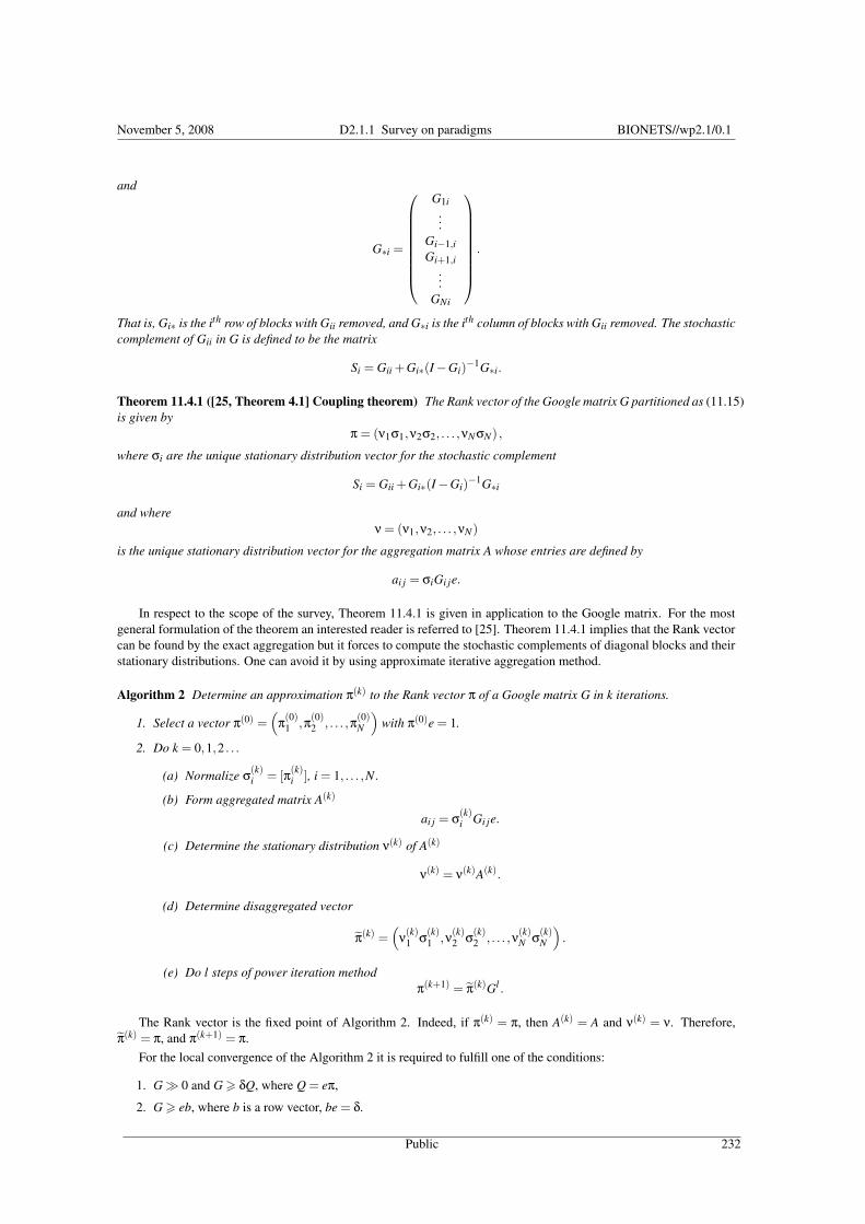
November 5, 2008 D2.1.1 Survey on paradigms BIONETS//wp2.1/0.1
and
G∗i =
G1i...
Gi−1,iGi+1,i
...GNi
.
That is, Gi∗ is the ith row of blocks with Gii removed, and G∗i is the ith column of blocks with Gii removed. The stochasticcomplement of Gii in G is defined to be the matrix
Si = Gii +Gi∗(I−Gi)−1G∗i.
Theorem 11.4.1 ([25, Theorem 4.1] Coupling theorem) The Rank vector of the Google matrix G partitioned as (11.15)is given by
π = (ν1σ1,ν2σ2, . . . ,νNσN) ,
where σi are the unique stationary distribution vector for the stochastic complement
Si = Gii +Gi∗(I−Gi)−1G∗i
and whereν = (ν1,ν2, . . . ,νN)
is the unique stationary distribution vector for the aggregation matrix A whose entries are defined by
ai j = σiGi je.
In respect to the scope of the survey, Theorem 11.4.1 is given in application to the Google matrix. For the mostgeneral formulation of the theorem an interested reader is referred to [25]. Theorem 11.4.1 implies that the Rank vectorcan be found by the exact aggregation but it forces to compute the stochastic complements of diagonal blocks and theirstationary distributions. One can avoid it by using approximate iterative aggregation method.
Algorithm 2 Determine an approximation π(k) to the Rank vector π of a Google matrix G in k iterations.
1. Select a vector π(0) =(
π(0)1 ,π(0)
2 , . . . ,π(0)N
)with π(0)e = 1.
2. Do k = 0,1,2 . . .
(a) Normalize σ(k)i = [π(k)
i ], i = 1, . . . ,N.
(b) Form aggregated matrix A(k)
ai j = σ(k)i Gi je.
(c) Determine the stationary distribution ν(k) of A(k)
ν(k) = ν(k)A(k).
(d) Determine disaggregated vector
π(k) =(
ν(k)1 σ(k)
1 ,ν(k)2 σ(k)
2 , . . . ,ν(k)N σ(k)
N
).
(e) Do l steps of power iteration methodπ(k+1) = π(k)Gl .
The Rank vector is the fixed point of Algorithm 2. Indeed, if π(k) = π, then A(k) = A and ν(k) = ν. Therefore,π(k) = π, and π(k+1) = π.
For the local convergence of the Algorithm 2 it is required to fulfill one of the conditions:
1. GÀ 0 and G > δQ, where Q = eπ,
2. G > eb, where b is a row vector, be = δ.
Public 232
November 5, 2008 D2.1.1 Survey on paradigms BIONETS//wp2.1/0.1
Since the Google matrix satisfies the both conditions, Algorithm 2 converges locally [24, Theorem 1]. Algorithm 2also converges globally if l is large enough [24].
Let us provide an estimation of the rate of convergence of Algorithm 2 [28].
1. Consider the condition G > δ1Q. Let us find δ1. Denote by gmin the minimum entry of the matrix G. If pi j = 0then gi j = gmin. Hence,
gmin =1− c
n. (11.17)
The maximum of the elements of the Rank vector π is achieved when all the other elements achieving minimum,because of π > 0 and πe = 1. The minimum entry of the Rank vector for a page is realized if there is no otherpage referring to it. The minimum entry of the Rank vector is 1−c
n . Therefore the maximum of one of the elementof the Rank vector is equal to
πmax = 1− 1− cn
(n−1) =1+ c(n−1)
n. (11.18)
Hence, if we find δ1 from the constraintgmin > δ1πmax, (11.19)
it ensures that G > δ1Q. From the equalities (11.17), (11.18) and (11.19) we get
δ1 6 1− c1+ c(n−1)
.
2. Consider the condition G > eb, where be = δ2. Let us determine δ2. From the equalities (11.6) we obtain, thatG > 1−c
n E. The equality can be rewritten as G > e( 1−c
n eT ). Therefore, as the vector b one can take
( 1−cn eT )
.Hence,
δ2 = 1− c.
The error vector of the method at the kth iteration is given by
π(k+1)−π = (π(k)−π)J(π(k)).
The definition and expressions for the matrix J(v) can be found in [24].From the above estimation and [24] we can conclude that the spectral radius of the matrix J(π):
1. is less than 1−δ1 = cn1+c(n−1) < 1,
2. is less than√
1−δ2 =√
c < 1.
For n big enough the second estimation becomes better than the first one. The second estimation ensures that theconvergence rate of the method is no less than
√c. Unfortunately, the estimation does not ensure that the method
converges faster than the power iteration method. Nevertheless, for the partial aggregation method which is discussedin the next subsection and is actually a particular case of the full aggregation method it was shown that there existssuch partitioning of the Google matrix which provides faster convergence than the convergence of the power iterationmethod.
11.4.3 Partial aggregation method (PAM)The partial aggregation method is considered in detail in [11]. Here we discuss the application of the method to theGoogle matrix and the Rank vector. The method is applied to the 2×2 case, i.e. N = 2, and the matrix G is partitionedas follows
G =(
G11 G12G21 G22
).
The matrix I−G is singular, but the matrix I−G11 is nonsingular [3]. Hence we can factor I−G = LDU [25, proof ofTheorem 2.3], where
L =(
I 0−G21(I−G11)−1 I
),
D =(
I−G11 00 I−S2
),
U =(
I −(I−G11)−1G120 I
),
Public 233
November 5, 2008 D2.1.1 Survey on paradigms BIONETS//wp2.1/0.1
and where S2 is a stochastic complement of the block G22.Since the matrix U is nonsingular we have π(I−G) = 0 if and only if πLD = 0. Hence
π2S2 = π2 π1 = π2G21(I−G11)−1, (11.20)
which means that π2 is a stationary distribution for the matrix S2. The expression (11.20) represents a particular caseof Theorem 11.4.1 for the 2× 2 decomposition of the transition matrix [25, Colorary 4.1]. The matrix S2 has uniquestationary distribution
σ2S2 = σ2, σ2e = 1.
And we can find π2 as π2 = ρσ2, where the factor ρ is chosen to satisfy the normalization condition πe = 1.The component π1 and the factor ρ can be expressed as components of the stationary distribution of the aggregated
matrix
A1 =(
G11 G12eσ2G21 σ2G22e
).
From (11.20), π2 = ρσ2 and σ2e = 1 we get
(π1,ρ)(I−A1) = 0, (π1,ρ)e = 1.
Since A1 is stochastic and irreducible [25, Teorem 4.1], it has a unique stationary distribution α,
αA2 = α, αe = 1.
By the uniqueness we get α = (π1,ρ).The above analysis implies that the Rank vector can be found by the partial exact aggregation but it forces to
compute the stochastic complement of G22, block of the Google matrix G and its stationary distribution. One can avoidthis by using the approximate iterative partial aggregation method.
Algorithm 3 Determine an approximation π(k) to the Rank vector π of a Google matrix G in k iterations.
1. Select a vector π(0) =(
π(0)1 ,π(0)
2
)with π(0)e = 1.
2. Do k = 0,1,2 . . .
(a) Normalize σ(k)2 = [π(k)
2 ].
(b) Form aggregated matrix A(k)1
A(k)1 =
(G11 G12e
σ(k)2 G21 σ(k)
2 G22e
).
(c) Determine the stationary distribution α(k) of A(k)1
α(k) = α(k)A(k)1 .
(d) Partition α(k)
α(k) = (ω(k)1 ,ρ(k)).
(e) Determine disaggregated vectorπ(k) =
(ω(k)
1 ,ρ(k)σ(k)2
).
(f) Do l steps of power iteration methodπ(k+1) = π(k)Gl .
Let us consider l = 1. Algorithm 3 is the power iteration methods with matrix G [11, Proposition 5.1, Theorem 5.2],where
G =(
0 0G21(I−G11)−1 S2
)
Therefore, the rate of convergence of Algorithm 3 is equal to |λ2(S2)| [11, Theorem 5.2]. If power iteration methodsconverges for matrix G then Algorithm 3 converges, too [11, Proposition 7.1]. If we consider a general stochastic matrixinstead of the Google matrix Algorithm 3 can converge slower than the power iteration method [11, Example 6.3], butfor the Google matrix there always exists such decomposition which ensures that Algorithm 3 converges faster than thepower iteration method.
Public 234
November 5, 2008 D2.1.1 Survey on paradigms BIONETS//wp2.1/0.1
11.4.4 BlockRank Algorithm (BA)The next method exploits the site structure of the Web. According to the experiments made by the authors of [18] themajority of links are the links between pages inside Web sites. Hence, we can decompose the set of pages I into thesubsets according to the Web sites, i.e. I (i) is the set of the pages of site i. Then, the Google matrix is partitionedaccording to the decomposition of I .
Algorithm 4 Determine an approximation π(k) to the Rank vector π of the Google matrix G in k iterations.
1. Determine local Rank vector for each diagonal block Pi
(a) Normalize Pi, i.e. (Pi) jk =(Pi) jk(Pi) j1
.
(b) Form Gi, Gi = cPi +(1− c)(1/n)E.
(c) Approximately determine πi
i. Select a vector π(0)i .
ii. Do k = 1,2 . . .
π(k)i = π(k−1)
i Gi.
2. Determine BlockRank
(a) Form aggregated matrix Aai j = πiPi je.
(b) Form B, B = cA+(1− c)(1/n)E.
(c) Approximately determine β
i. Select a vector β(0).ii. Do k = 1,2 . . .
β(k) = β(k−1)B.
3. Determine global Rank vector
(a) Form the vector π(0) = (β1π1,β2π2, . . . ,βN πN).
(b) Do k = 1,2 . . .π(k) = π(k−1)G.
It was empirically shown that Algorithm 4 is faster than the power iteration method by at least the factor of two[18].
11.4.5 Fast Two-Stage Algorithm (FTSA)The next method also exploits the structure of the Web and in particular the presence of dangling nodes [23]. The mainidea of the method is to lump dangling nodes into one state and find the Rank vector of the new aggregated matrixat the first stage and to aggregate non-dangling pages into one state at the second stage. Therefore, the set of pagesis decomposed into two sets I1 and I2, where I1 ∪ I2 = I , and I1 contains all non-dangling pages and I2 contains alldangling pages. Hence, the matrix G is represented in the following way:
G =(
G11 G12en1 vn1 en2 vn2
),
where e =(eT
n1,eT
n2
)T and v = (vn1 ,vn2).
Algorithm 5 Determine an approximation π(k) to the Rank vector π of the Google matrix G in k iterations.
1. The first stage: lump dangling pages
(a) Form the lumped matrix G(1)
G(1) =(
G11 G12en2
vn1 vn2 en2
).
(b) Approximately determine π1
Public 235

November 5, 2008 D2.1.1 Survey on paradigms BIONETS//wp2.1/0.1
i. Select a vector π(0)1 .
ii. Do k = 1,2 . . .
π(k)1 = π(k−1)
1 G(1).
(c) Determine aggregation weights of the second stage
η =π1
∑n1i=1(π1)i
.
2. The second stage: aggregate non-dangling pages
(a) Form aggregated matrix G(2)
G(2) =(
ηG11en1 ηG12vn1 en1 en2 vn2
).
(b) Approximately determine π2
i. Select a vector π(0)2 .
ii. Do k = 1,2 . . .
π(k)2 = π(k−1)
2 G(2).
3. Form the Rank vectorπ = (π1,π2) .
The first stage requiring less computation work than the power iteration method does, roughly O(n1) as opposed toO(n) per iteration, and converges at least as fast as the power iteration method. The second stage usually converges toafter about three iterations. If the second stage does not converge after about three iterations the acceleration based onAitken Extrapolation [19] can be applied:
(π2)i =
((π(2)
2
)i−
(π(1)
2
)i
)2
(π(3)
2
)i−2
(π2)
2
)i+
(π(1)
2
)i
.
11.4.6 Distributed PageRank Computation (DPC)
The following method is designed for distributed computation of the Rank vector [35]. The set of pages is decomposedby sites, i.e. I (i) is the pages of site i. The main idea of the method is to allow each site to compute the Rank vector forlocal pages and after that construct the entire Rank vector. (We refer to a site as a super-node which can independentlyperform computations.) After the Rank vectors for local pages is constructed by each super-node, the vectors are sentto selected central node (for example, central node can be one of the super-nodes), which constructs an aggregatedmatrix and determines its stationary distribution. The entries of the aggregated stationary distribution are delivered tosuper-nodes each of which constructs extended local transition matrix. Super-node determine stationary distribution ofthe extended local transition matrix and a part of the stationary distribution is normalized and reported to central node.The process is repeated until convergence. The formal definition of the algorithm is the following.
Let S(π) denote a N×n disaggregation matrix as
S(π) =
S(π)1 0 . . . 00 S(π)2 . . . 0...
.... . .
...0 0 . . . S(π)N
,
where S(π)i = [πi] is a row vector denoting the censored stationary distribution of pages in site i. Also let us denote byGi the ith block row of the matrix G partitioned as (11.15), i.e.
Gi = (Gi1,Gi2, . . . ,GiN) .
Algorithm 6 Determine an approximation π(k) to the Rank vector π of the Google matrix G in k iterations.
1. For each super-node i
Public 236

November 5, 2008 D2.1.1 Survey on paradigms BIONETS//wp2.1/0.1
(a) Construct an ni×ni local transition matrix Gii, i.e. normalize Gii
(Gii
)jk =
(Gii) jk
(Gii) j 1.
(b) Determine the stationary distribution π(0)i for Gii.
2. Do k = 0, 1, 2, . . .
3. the central node
(a) Normalize σ(k)i = [π(k)
i ].
(b) Construct the aggregated matrix A(k) with
ai j = σ(k)i Gi je.
(c) Determine the stationary distribution ν(k) for A(k).
4. For each super-node i
(a) Construct an (ni +1)× (ni +1) extended local transition matrix
B(k)i =
Gii eT (I−Gii
)(
ν(k)S(π(k))Gi−ν(k)i π(k)
i Gii
)
1−ν(k)i
αk
,
where the scalar αk ensures the row sum of B(k)i is one.
(b) Determine the stationary distribution bki for B(k)
i .
(c) Partition bki
bki = (ω(k)
i ,β(k)i ),
where β(k)i is a scalar.
(d) Form local vector π(k)i
π(k)i =
1−ν(k)i
β(k)i
ω(k)i .
5. The central node
(a) Construct vector π(k)
π(k) =(
π(k)1 , π(k)
2 , . . . , π(k)N
).
(b) Normalize π(k) = [π(k)].
The method is proved to be equivalent to iterative aggregation/disaggregation method based on Block Jordan de-composition [35]. The main advantage of this method is that it provides a distributed way to calculate the Rank vector,at the same time the communication overhead is not high due to only scalars and vector are being sent between nodesand not matrices. The entire communication overhead is of the magnitude O(nnz((L +U)S(π)))+ O(n), where L andU are low-triangular and upper-triangular matrices of the matrix P, respectively.
11.4.7 Discussion of the A/D methodsThe considered A/D methods can be classified into two groups. While FAM and PAM are general methods which canbe applied to any decomposition of the set of nodes, BA and FTSA propose to use a particular decomposition. Therate of convergence of FAM and PAM essentially depends on the chosen decomposition. The questions of “optimal”decomposition of the set of nodes and convergence acceleration are still not fully answered. BA and FTSA methods havemade a step in the direction of solving the both questions. Whilst the BA method accelerates the power iteration method,the FTSA method converging as fast as the power iteration method reduces the dimension of matrices and vectorsused in iterations. The DPC method, being distributed and parallel method, converges like aggregation-disaggregationmethod and at the same time has low communication overhead.
Public 237
November 5, 2008 D2.1.1 Survey on paradigms BIONETS//wp2.1/0.1
11.5 Personalized approachThe above presented algorithms compute the global reputation measure. Namely, to calculate the Rank vector we needan input (may be indirect) from all the nodes. However, the reputation discounts quickly in the chain of acquaintances.This provides a motivation to consider “localized” or “personalized” versions of the graph based reputation measures.Furthermore, one often needs to encompass different notions of importance or reputation for different users and queries.Thus, the original algorithm should be modified to take into account personalized view for the reputation of the nodes.
As we mentioned in the introduction, in general a random walk follows the outgoing links with probability c, andmakes a random jump with probability (1− c) according to the probability distribution given in v. Depending on the“type” of users, vector v will not be uniform, but biased to some set of nodes, which are considered to be importantfor these “types” of users. For this reason, the vector v is referred as personalization vector. Let π(v) denote thepersonalized Rank vector (PRV), corresponding to the personalization vector v. It can be computed by solving theequation π = πG
π = πcP+(1− c)v,
π−πcP = (1− c)v,
π(I− cP) = (1− c)v.
Since c is different from one, the matrix (I− cP) is invertible and we have
π(v) = v(1− c)(I− cP)−1. (11.21)
Let Q = (1− c)(I− cP)−1. By letting v = eTi
1 we see that π(ei) = Qi− the ith row of Q. Thus, rows of Q comprise acomplete basis for personalized Rank vectors. Any PRV can be expressed as a convex linear combination of these basicvectors. This statement is based on the following theorem:
Theorem 11.5.1 Given two arbitrary π1,π2 PRVs and v1,v2 are their corresponding personalization vectors. Then,for any constants α1,α2 > 0 such that α1 +α2 = 1
α1π1 +α2π2 = c(α1π1 +α2π2)P+(1− c)(α1v1 +α2v2) (11.22)
For any personalization vector v, the corresponding PRV is given by : vQ. Unfortunately, approach to use the completebasis for the personalized Rank vector is infeasible in practice. Computing the dense matrix Q off line is impracticaldue to its huge size. However, rather than using the full basis, we can use a reduce basis with k < n vectors. In this case,we can not express all PRVs but only those corresponding to convex combinations of the vectors in reduced basis set
π(ω) = wQ. (11.23)
11.5.1 Scaled PersonalizationIn [16] the authors have presented a method that enables the computation of PRVs which scales well with the increasingnumber of users. The authors of [16] have developed their method in the context of information retrieval. Then, theauthors of [7] have adopted the method of [16] to the reputation management in P2P networks. In this survey, we alsopresent a broader reputation measure based interpretation of the algorithm of [16]. We would like to mention that thedivision of the users in two groups: pre-trusted peers and regular users provide yet another application of the results of[7, 16] in the context of Bionets [4].
The central notion of the scaled personalization algorithm is the set of pre-trusted peers (or hub peers). A regularpeer can choose some of pre-trusted peers. This does not mean that the hub peers selected by a user more trustworthythan the other hub peers. This simply means that a user might prefer certain hub peers because they supply a specificservice of a very good quality. Next let us describe several stages of the scaled personalization algorithm.
Specification Let us consider a set of the personalization vectors uh where uh = eh is biased to a specific hub nodeh ∈ H. We denote by H the set of hub nodes. The personalized Rank vector corresponding to uh is called a basis hubvector πh. If the basis vector for each hub node h ∈ H is computed and stored, then, by Theorem 11.5.1 any PRVcorresponding to a preference set P ⊆ H can be computed. The preference set P corresponds to the set of hub nodeschosen by a user as preferred pre-trusted peers.
Each hub vector can be computed naively by power method. However, this task is very expensive in time andresources. The algorithm of [16] enables a more scalable computation by constructing hub vectors from shared compo-nents.
1ei has 1 in ith place, and 0 elsewhere.
Public 238

November 5, 2008 D2.1.1 Survey on paradigms BIONETS//wp2.1/0.1
Decomposition of Basis Vectors To compute a large number of basis hub vectors efficiently, one can decomposethem into partial vectors and hubs skeleton, components from which hub vectors can be constructed quickly.
Let define the inverse P-distance r′p(q) from p to q as
r′p(q) = ∑t:pÃq
P[t](1− c)cl(t), (11.24)
where the summation is taken over all tours t, starting from p and finishing at q, possibly visiting p and q more thanone time, l(t) is the length of the tour, and P[t] is the probability of taking the tour t.
Consider tour t =< w1, . . . ,wk >, then
P[t] =k−1
∏i=1
1Outdeg(wi)
,
or 1, if l(t) = 0. If there is no any tours from p to q, the summation is taken to be equal to 0. It is proven thatπp(q) = rp(q) [16].
Let us also define the restricted inverse P-distance. Let H ⊆V be some nonempty set of nodes. For p,q ∈V , rHp (q)
is defined as a restriction of rp(q) that considers only tours from p to q that pass through H, that is,
rHp (q) = ∑
t:pÃHÃqP[t](1− c)cl(t). (11.25)
Intuitively, rHp (q) is the influence of p on q through H. Obviously, if all paths from p à q come through H, then
rHp (q) = rp(q). For carefully chosen H, rp(q)− rH
p (q) = 0 for many pages p,q. The strategy is to take advantage of thisproperty by breaking rp into components (rp− rH
p ) and rHp .
πp = rp = (rp− rHp )+ rH
p . (11.26)
The vector (rp− rHp ) is called the partial vector. Computing and storing partial vectors is cheaper, since they can be
represented as a list of their nonzero entries. Moreover, the size of each partial vector will decrease as H increases insize, making this approach particularly scalable. It can be proven that any rH
p vector can be expressed in terms of thepartial vectors (rh− rH
h ) for h ∈ H (see the Hub Theorem in [16]).
Theorem 11.5.2 For any p ∈V,H ⊆V ,
rHp =
11− c ∑
h∈H(rp(h)− (1− c)xp(h))(rh− rH
h − (1− c)xh), (11.27)
where xh = eh. The quantity (rh− rHh ) appears on the right hand side of (11.27) is the partial vector. Suppose we have
computed rp(H) = (h,rp(h))|h ∈ H for a hub node p. Substituting it into equation (11.26) gives
rp = (rp− rHp )+
11− c ∑
h∈H(rp(h)− (1− c)xp(h))[(rh− rH
h )− (1− c)xh]. (11.28)
The equation is central to the construction of hub vectors from partial vectors. The set S = rp(H)|p ∈ H formsthe hubs skeleton, giving the interrelationships among partial vectors. Computing (rp− rH
p ), p ∈ H naively by powermethod is inefficient due to the large number of hub nodes. Three scalable algorithms for computing these partialvectors, using dynamic programming are presented. All of them are based on the decomposition theorem in [16].
Theorem 11.5.3 For any p ∈V
rp =c
|O(p)||O(p)|∑i−1
rOi(p) +(1− c)xp (11.29)
where Oi(p) is the ith neighbour of node p.
The above theorem gives the interpretation for PRV. The p’s view of rp is the average of the views of its out-neighbors,but with extra importance given to p itself.
Public 239

November 5, 2008 D2.1.1 Survey on paradigms BIONETS//wp2.1/0.1
Construction of PRV’s Let u = α1 p1 + . . .+az pz be a preference vector, where pi ∈ H. Let
ru(h) =z
∑i=1
αi(rpi(h)− c.xpi(h)). (11.30)
Then, the PRV π can be computed as follows:
π =z
∑i=1
αi(rpi − rHpi)+
11− c ∑
h∈Hru(h)[(rh− rH
h )− (1− c)xh]. (11.31)
The choice of H The choice of hub nodes can have a strong effect on the overall performance. Particularly, the sizeof partial vectors is smaller when pages in H have high Rank vector values, since nodes with high Rank vector valuesare closer in term of P-reverse distance to other pages. In the context of P2P networks, it is natural for the members inthe pre-trusted peers to have high Rank values.
11.5.2 Relation to the A/D approachLet us relate the Personalized Rank vector approach to the A/D approach. The BlockRank algorithm proposed in [18]computes n× k matrix corresponding to k blocks. Each block corresponds to a host. Instead of choosing an uniformdistribution over pages to which the user jumps, we may choose a distribution centered on hosts. So, we can encodethe personalization vector in the k-dimensional space. With this adaptation the local Rank vector will not change fordifferent personalizations. Only the BlockRank depends on the personalizations. Therefore, we only need to recomputethe BlockRank for each block-personalization vector. The BlockRank algorithm is able to exploit the graph’s blockstructure to compute efficiently many of the block-oriented basis vectors.
11.6 ConclusionsIn this paper we reviewed reputation and trust measures that one can apply to BIONETS. Graph based reputationmeasures are discussed in details. Although all the methods can be effectively implemented in BIONETS environments,some of them has evident advantages and disadvantages. Aggregation/disaggregation methods like FAM, PAM, BA,DPC construct an aggregated matrix and its stationary distribution at each iteration of the algorithms that requirescommunication with selected central node. In application to BIONETS it means that before the iterations can becontinued all the "islands" should connect to a selected node (which means there should be a node traveling to theselected nodes and back to an "island") to upload current state and, after a while, connect the same selected node todownload aggregated distribution. This constraint is very stringent for BIONETS systems since it requires existence ofnodes with special mobility pattern. Besides the mentioned disadvantages BA and DPC has an advantage over FAM,PAM and FTSA since BA and DPC calculate local Rank vectors as an initialization to iterations that can be used asreputation before islands get a connection to the selected node and determine the global reputation. The asynchronousapproach and Monte Carlo method take an advantage comparing to aggregation/disaggregation methods since a lot ofcalculation of reputation can be done inside an island and the information of local reputation can be spread to otherislands by nodes traveling occasionally from one island to another. While the spreading of information is achieved bymerging generated random walks in Monte Carlo method, in asynchronous approach it is done by choosing appropriatefunctions of U(t) and d(t, i, j), where U(t) is responsible for reachable at the moment nodes and d(t, i, j) defines relativeage of reputation values used in further calculations. Personalized approach is a kind of auxiliary approach to all thediscussed methods because it chooses personalization vector that can be used in aggregation/disaggregation methods aswell as in the asynchronous approach and the Monte Carlo method. The personalized approach allows one to take intoaccount preferences like special services provided by nodes or extremely high quality of common services.
Public 240

Bibliography
[1] K. Avrachenkov and N. Litvak. “Decomposition of the Google PageRank and Optimal Linking Strategy”. INRIAResearch Report no. 5101, 2004.
[2] K. Avrachenkov, N. Litvak, D. Nemirovsky and N. Osipova, “Monte Carlo methods in PageRank computation:When one iteration is sufficient”, SIAM Journal on Numerical Analysis, v.45, no.2, pp.890-904, 2007.
[3] A. Berman and R.J. Plemmons. “Nonnegative Matrices in the Mathematical Sciences”. SIAM Classics In AppliedMathematics, SIAM, Philadelphia, 1994.
[4] Biologically inspired Network and Services (BIONETS): http://www.bionets.org/
[5] L.A. Breyer, “Markovian Page Ranking Distributions: Some Theory and Simulations”, Technical report, 2002;available online at http://www.lbreyer.com/preprints.html.
[6] D. Chazan and W.L. Miranker, “Chaotic relaxation”, Linear Algebra and its Applications, v.2, pp.199-222, 1969.
[7] P.A. Chirita, W. Nejdl, M. Schlosser, and O. Scurtu, “Personalized reputation management in P2P networks”, inProceedings of the Trust, Security, and Reputation Workshop, 2004.
[8] L. Eschenauer, V. Gligor and J. Baras, “On trust establishment in mobile Ad Hoc networks”, in Proceedings ofSecurity Protocols Workshop, pp.47-66, 2002.
[9] I. Foster and C. Kesselman, (eds.) “The GRID: Blueprint for a new computing infrastructure”, Elsevier, SanFrancisco, 2004.
[10] Z. Gyongyi, and H. Garcia-Molina and J. Pedersen, “Combating Web Spam with TrustRank”, VLDB, Toronto,Canada, 2004.
[11] C.F. Ipsen and S. Kirklad. “Convergence analysis of an improved PageRank algorithm”. NCSU CRSC TechnicalReport, 2004.
[12] T.H. Haveliwala, “Topic-Sensitive PageRank”, in Proceedings of the 11th International World Wide Web Confer-ence, 2002.
[13] T.H. Haveliwala and S.D. Kamvar, “The Second Eigenvalue of the Google Matrix”, Stanford University TechnicalReport, March 2003.
[14] D. de Jager, “PageRank: Three distributed algorithms”, Master thesis, Imperial College (University of London),2004.
[15] D. de Jager and J.T. Bradley, “Asynchronous iterative solution for state-based performance metrics”, in Proceed-ings of ACM SIGMETRICS 2007.
[16] G. Jeh and J. Widom, “Scaling Personalized Web Search”, in Proceedings of the 12th International World WideWeb Conference, 2003.
[17] A. Josang, R. Ismail and C. Boyd, “A survey of trust and reputation systems for online service provision”, DecisionSupport Systems, v.43, no.2, pp.618-644, 2007.
[18] S. Kamvar, T. Haveliwala, C. Manning, and G. Golub. “Exploiting the block structure of the web for computingpagerank”. Stanford University Technical Report, 2003.
[19] S.D. Kamvar, T.H. Haveliwala, C.D. Manning, and G.H. Golub, “Extrapolation methods for accelerating PageR-ank computations”, in Proceedings of the 12th International World Wide Web Conference, 2003.
[20] S.D. Kamvar, M.T. Schlosser and H. Garcia-Molina, “The EigenTrust algorithm for reputation management inP2P networks”, in Proceedings of the 12th International World Wide Web Conference, 2003.
241

November 5, 2008 D2.1.1 Survey on paradigms BIONETS//wp2.1/0.1
[21] G. Kollias, E. Gallopoulos and D. Szyld, “Asynchronous iterative computations with Web information retrievalstructures: The PageRank case”, in Proceedings of the International Conference ParCo 2005. Parallel Computing:Current & Future Issues of High-End Computing, pp.309-316.
[22] A.N. Langville and C.D. Meyer. “Deeper inside pagerank”. Internet Mathematics, 1(3):335–380, 2005.
[23] Ch.P.Ch. Lee, G.H. Golub, and S.A. Zenios, “A fast two-stage algorithms for computing PageRank”, SCCMReport, 2002.
[24] I. Marek and I. Pultarova. “Two notes on local and global convergence analysis of iterative aggregation-disaggregation method” available on the Web, 2005.
[25] C.D. Meyer and R.J. Plemmons. “Stochastic complementation, uncoupling Markov chains, and the theory ofnearly reducible systems”. SIAM Rev., 1989.
[26] C.B. Moler. “Numerical Computing with MATLAB”. SIAM, 2004.
[27] L. Mui, M. Mohtashemi and A. Halberstadt, “A computational model of trust and reputation”, in Proccedings ofthe 35th Hawaii International Conference on System Sciences, 2002.
[28] D.A. Nemirovsky, “Analysis of iterative methods for PageRank computation based on decomposition of the Webgraph”, Master thesis, St.Petersburg State University, in Russian, 2005.
[29] The Open Directory Project www.dmoz.org
[30] L. Page, S. Brin, R. Motwani and T. Winograd, “The PageRank citation ranking: Bringing order to the Web”,Technical Report, Stanford Digital Library Technologies Project , 1998.
[31] K. Sankaralingam, S. Sethumadhavan and J.C. Browne, “Distributed pagerank for P2P systems”, in Proceedingsof the 12th IEEE International Symposium on High Performance Distributed Computing, 2003.
[32] S.M. Shi, J. Yu, G.W. Yang and D.X. Wang, “Distributed page ranking in structured P2P networks”, in Proceedingof International Conference on Parallel Processing, 2003.
[33] W.J. Stewart. “Introduction to the numerical solutions of Markov chains”. Princeton University Press, Princeton,1994.
[34] A. Yamamoto, D. Asahara, T. Itao, S. Tanaka and T. Suda, “Distributed pagerank: a distributed reputation modelfor open peer-to-peer network”, in Proceedings of the International Symposium on Applications and the InternetWorkshops, 2004.
[35] Y. Zhu and Sh. Ye and X. Li, “Distributed PageRank computation based on iterative aggregation-disaggregationmethods”, in CIKM ’05: Proceedings of the 14th ACM international conference on Information and knowledgemanagement, 2005, an updated version is available at http://www.cs.cmu.edu/˜yangboz/cikm05_pagerank.pdf.
[36] C.-N. Ziegler and G. Lausen, “Spreading activation models for trust propagation”, in Proceedings of IEEE Inter-national Conference on e-Technology, e-Commerce and e-Service, 2004.
[37] C.-N. Ziegler and G. Lausen, “Propagation models for trust and distrust in social networks”, Information SystemsFrontiers, v.7, no.4/5, pp.337-358, 2005.
[38] S. Buchegger and J.-Y. L. Boudec. Performance analysis of the confidant protocol. In MobiHoc ’02: Proceedingsof the 3rd ACM international symposium on Mobile ad hoc networking & computing, pages 226–236, Lausanne,Switzerland, 2002.
[39] S. Buchegger and J.-Y. L. Boudec. A robust reputation system for P2P and mobile ad-hoc networks. In SecondWorkshop on the Economics of Peer-to-Peer Systems, Cambridge, MA, USA, 2004.
[40] Z. Despotovic and K. Aberer. P2P reputation management: probabilistic estimation vs. social networks. ComputerNetworks, 50(4):485–500, 2006.
[41] A. Garg, R. Battiti, and G. Costanzi. Dynamic Self-management of Autonomic Systems: The Reputation, Qualityand Credibility (RQC) scheme. In The 1st IFIP TC6 WG6.6 International Workshop on Autonomic Communica-tion (WAC 2004) (LNCS 3457), pages 165–176, Berlin, Germany, Oct. 2004. Springer.
[42] P. Resnick and R. Zeckhauser. Trust among strangers in internet transactions: Empirical analysis of ebay’s rep-utation system. the economics of the internet and e-commerce. In M. R. Baye, editor, Advances in AppliedMicroeconomics, volume 11, pages 127–157. Elsevier Science, 2002.
[43] L. Xiong and L. Liu. PeerTrust: Supporting reputation-based trust in peer-to-peer communities. IEEE Transac-tions on Data and Knowledge Engineering, Special Issue on Peer-to-Peer Based Data Management, 16(7):843–857, July 2004.
Public 242

November 5, 2008 D2.1.1 Survey on paradigms BIONETS//wp2.1/0.1
[44] R. Cascella and A. Garg (Eds.). Trust and reputation management system definition. BIONETS (IST-2004-2.3.4FP6-027748) Deliverable (D4.1), June 2007.
[45] D. Schreckling (Eds.). Towards security in BIONETS. BIONETS (IST-2004-2.3.4 FP6-027748) Deliverable(D4.2), August 2007.
[46] S. Capkun, J.-P. Hubaux, and L. Buttyán. Mobility helps peer-to-peer security. IEEE Transactions on MobileComputing, 5(1):43–51, January 2006.
Public 243

November 5, 2008 D2.1.1 Survey on paradigms BIONETS//wp2.1/0.1
Public 244
Chapter 12
Network Formation GamesGiovanni Neglia
Abstract. Recent research in different fields like physics, economics, social sciences has pointed out the important roleof network structure for the performance of a distributed system (be it a group of friends, the World Wide Web or abusiness and commerce system). In current Internet the network structure arises from interactions of agents at differentlevels. Internet Service Providers (ISPs) and different organizations decide autonomously which other entities in theInternet they want to be directly connected to. More recently Peer-to-Peer (P2P) networks and ad hoc networks haveintroduced new actors shaping the current Internet structure. All these agents (ISPs, peers,...) may have disjoint andcompeting interests, so game theory can provide useful mathematical tools to study the outcomes of their interactions.In particular there is a growing research trend on so-called network formation games, which explicitly consider playerswho can decide to connect to each other. In these games the network structure both influences the result of the economicinteractions and is shaped by the decisions of the players. The purpose of this chapter is to provide the reader unfamiliarwith this research area with the basic concepts, pointers to other surveys, and an overview of current results in thecomputer networks field.
12.1 IntroductionRecent research in different fields like physics, economics, social sciences has pointed out the important role of networkstructure for the performance of a distributed system (would it be a group of friends, the World Wide Web or a businessand commerce system). The birth of a new science of networks has been advocated [6].
In current Internet the network structure arises from interactions of agents at different levels. First regarding thephysical infrastructure of traditional wired Internet, there is no single central authority designing the graph, but InternetService Providers (ISPs) and different organizations decide autonomously which other entities in the Internet they wantto be directly connected to, and the use of the link established (e.g. if these links can forward also third party traffic andif so at which price).
New scenarios are extending the number of actors involved in shaping the current Internet structure. Peer-to-Peer (P2P) networks and ad hoc networks clearly show this trend. P2P applications rely on overlays, i.e. logicalnetworks, built atop of the existing physical infrastructure. Connections among nodes are logical or virtual links atthe application level, so an end user interacts with other users in order to create the logical network. Current overlaysexhibit different topologies, like stars, rings, d-dimensional grids, butterflies, de Bruijn graphs, trees, and random graphgenerated topologies. The wide spectrum of proposed solutions reveals by itself that there is no optimal choice for allpossible design goals like robustness, maintenance costs, efficiency for routing and efficiency for dissemination. Adhoc networks are formed by nodes (like laptops or sensors) with wireless transmission capabilities located in a givearea, in general without any backbone infrastructure to route packets. For this reason nodes have to act as routers andto cooperate to deliver traffic in the network. They can create a specific topology, because they have the possibility -toa given extent- to determine the set of reachable nodes, by deciding for example their power transmission level and theorientation of the antenna and which nodes they want to forward the traffic to among those reachable.
Endogenous network formation is probably going to play a more and more important role in future computernetworks. This is a particular aspect of current attrition of central and explicit control. In fact computer networksare rapidly increasing in size and extending to new environments (vehicles, home appliances, natural ecosystems...).
245

November 5, 2008 D2.1.1 Survey on paradigms BIONETS//wp2.1/0.1
Central and explicit control is not a feasible solution for the management and operation of these large scale distributedsystems. Even traditional approaches to distributed system design are not applicable as they would not scale to suchsizes, nor would they be able to deal with the fast dynamics and the intrinsic unreliability of the components of thesesystems. For example in P2P networks and ad hoc and sensor networks new nodes can join the system while othersleave abruptly because of users decisions or failures (e.g. due to battery depletion). At the same time mobility andvagaries of wireless channel can frequently sever and create links. In some cases even connectivity across the networkcannot be assumed: in Delay Tolerant Networks disconnected operation is the normal situation rather than an exception.These issues call for completely distributed self-organizing systems, i.e. systems able to reorganize themselves on thebasis of local knowledge to deal with such dynamic environment. The absence of a central server (or of central servers)intrinsically offers more robustness to failures. Also, completely decentralized systems appear intrinsically appealingto implement communication, storage and computational services in a bottom-up fashion, at a very low cost. Besidesthese technological motivations, the popularity of P2P applications among Internet users also strengthen this tendencyto decentralization.
In general, altruistic cooperation cannot be assumed in computer networks, where users likely have disjoint andcompeting interests, and this is also true for network formation. This is clear for ISPs, that are primarily concernedwith maximizing profits. But also users in a P2P networks can have specific interests in controlling the number ofconnections they establish (because they can be costly), or in establishing some connections rather than others, e.g. toincrease their downloading rate in a file-sharing network, or to achieve a better quality in a multicast overlay for real-time contents. Also the behavior of nodes in an ad hoc network can be driven by the wish to spare their own battery,avoiding to cooperate in the forwarding process. Decentralization makes these issues more significant, because in adecentralized environment it is harder to force users to cooperate. Game theory is clearly a candidate to study such kindof problems, because it provides mathematical tools to study the outcomes of interactions among self-interested players.In particular there is a growing research trend in game theory on so-called network formation games, which explicitlyconsiders players who can decide to connect to each other. In these games the network structure both influences theresult of the economic interactions and is shaped by the decisions of the players. Characterizing the structure and theefficiency of networks arising as equilibria from players interaction is one of the main purpose of such research.
12.2 Purpose and outline
The purpose of this document is not to be an exhaustive survey on network formation games techniques and applications,but rather to provide the reader unfamiliar with this research area with the basic concepts, pointers to other surveys, andan overview of current results in the computer networks field.
The chapter is organized as follows. In section 12.3 we introduce the two main approaches in current researchon network formation games research adopted from two different different communities. In section 12.4 we illustratethe main concepts and tools used in this research field. Finally in section 12.5 we present papers addressing networkformation problems in computer networks.
12.3 Approaches
The birth of network formation games can be dated to 1977 with Myerson’s paper [24]. Since that time networkformation games have been applied as models of social and economic networks focusing on pairwise relations betweenindividuals or companies who can locally form direct links. In this research stream link creation usually requiresagreement among the players, so new equilibria concepts have been developed to address this coordination requirement(see section 12.4). An optimal survey of this socio-economic literature is [16].
More recently there has been an increasing interest on network formation games from researchers in theoreticalcomputer science, interested in the fusion of algorithmic ideas with concepts and techniques from game theory. Thisnew research area is sometimes referred to as algorithmic game theory. Algorithmic game theory focuses mainlyon computational issues in game theory, like Nash equilibrium or best response computation or mechanism design.Useful introductions to this field are [27, 15], while the first book on this subject has appeared recently [1]. Up tonow algorithmic game theory has given a specific contribution to network formation games with the elaboration ofprice of anarchy and price of stability concepts to quantify the cost of using decentralizing solution to a problem (seesection 12.4). In [29] the author presents some illustrative results on network formation games fitting them in moregeneral frameworks (congestion games, potential games and utility games) and introducing open research issues.
Public 246

November 5, 2008 D2.1.1 Survey on paradigms BIONETS//wp2.1/0.1
12.4 Main Concepts in Network Formation GamesIn this section we are going to introduce some important concepts in network formation games, using a simple exampleas starting point.
Let us assume that there are N players and the strategy of each player is the set of links he would like to create withother players. Formally we indicate the strategy of player i with the vector si, where si, j = 1 indicates his willingnessto form a link with player j, si, j = 0 otherwise. The set of possible strategies is than Si = 0,1N . We denote the linkbetween i and j as i j and we assume that the link between i and j is created when one of the two players wants it, i.e. ifsi, j ∨ s j,i = 1. Given a strategy profile s, we indicate the network rising from player interaction as g(s), which is simplythe list of unordered pair of connected players, and we indicate as G the set of all possible networks users can form.With some abuse of notation, we let i j ∈ g indicate that link i j belongs to the network g and we let also g + i j denotethe network found by adding the link i j to the network g and g− i j denote the network found by deleting the link i jfrom the network g. The utility of player i is a function of the final network g, we denote it as ui(g).
For example in [13] user utility takes into account the cost of the number of connections established with otherplayer -|si| for user i- as well as the sum of the costs of reaching all the other players:
−ui(g(s)) = α|si|+N
∑j=1
d(i, j)(g(s)), (12.1)
where d(i, j)(g(s)) is the shortest-path distance (in terms of hops-count) between nodes i and j in the graph g(s).
12.4.1 Nash EquilibriumA standard equilibrium concept in Game Theory is Nash equilibrium. With reference to our example above we say thata strategy profile s∗ is a Nash Equilibrium if
∀i,∀si ∈ Si, ui(g(s∗))≥ ui(g(si,s∗−i)),
where (si,s∗−i) indicates a strategy profile s′ such that s′j = s∗j ∀ j 6= i, and s′i = si. This is a Nash equilibrium in purestrategies, mixed strategies are not usually considered in network formation games literature.
A network g is said to be Nash stable if it arises from a Nash equilibrium.Sometimes also approximate Nash equilibria are considered. Roughly speaking an approximate Nash equilibrium
is a strategy profile, such that users convenience to defect is smaller than a given bound. In case of absolute improvementbounds, s∗ is a ε-approximate Nash Equilibrium (with ε > 0) if
∀i,∀si ∈ Si, ui(g(s∗))≥ ui(g(si,s∗−i))− ε,
while in case of relative improvement bounds, s∗ is a ε-approximate Nash Equilibrium (with 1 > ε > 0) if
∀i,∀si ∈ Si, ui(g(s∗))≥ ε ui(g(si,s∗−i)).
Approximate Nash equilibria have been advocated as tools to quantify the lack of coordination due to selfishbehaviour (section 12.4.4) when Nash equilibria do not exist, or are hard to find.
12.4.2 Other Equilibria for Coordination requirementIn socio-economic literature it is common to consider situations when both players have to agree in order to create alink. For example with reference to our reference game, a link would be created only if si, j ∧ si, j = 1.
In such cases the concept of Nash equilibrium can be inadequate, because it allows for too many equilibria. Forexample the empty network is always a Nash stable network regardless of the utility functions ui(). In order to deal withthis coordination requirement new equilibria concepts have been introduced. Here we mainly follow the terminologyin [7], where also relations among these different equilibria are illustrated.
Pairwise Stable Networks
A network g is pairwise stable if
a) ∀i j ∈ g, ui(g)≥ ui(g− i j),
b) ∀i j 6∈ g, if ui(g+ i j) > ui(g) then u j(g+ i j) < u j(g).
Then the network is not pairwise stable if some player can gain by deleting a link or two players can gain from addinga link. Note that the concept of pairwise stability does not consider more complex deviations where for example a nodecan sever two or more links at the same time.
Public 247
November 5, 2008 D2.1.1 Survey on paradigms BIONETS//wp2.1/0.1
Pairwise Nash Stable Networks
Nash equilibrium and pairwise stability can be merged together. We say that a strategy set s∗ is a pairwise Nashequilibrium if
a) s∗ is a Nash equilibrium,
b) ∀i j 6∈ g, if ui(g+ i j) > ui(g) then u j(g+ i j) < u j(g).
A network g is pairwise Nash stable if there exists a pairwise Nash equilibrium s of the game, such that g = g(s)1.
Allowing transfers
If transfer among players are allowed than the previous definition can be straightforwardly extended. Here we onlypresent the concept of a pairwise stable network with transfers, the reader can refer to [7] for the other extensions.
A network g is said to be pairwise stable with transfers if
a) ∀i j ∈ g, ui(g)+u j(g)≥ ui(g− i j)+u j(g− i j)
b) ∀i j 6∈ g, ui(g)+u j(g)≥ ui(g+ i j)+u j(g+ i j).
12.4.3 Value Function and Allocation RuleValue function and allocation rule are natural extensions of characteristic function and imputation rule from the coop-erative game theory (see for example [28] for a gentle introduction to these concepts).
The value function assigns a value to every possible network players can create, v : G→ R. The set of all possiblevalue functions is denoted by V . The value of a network can in general depend in arbitrary ways on the structure of thenetworks, but component additivity and anonymity are common assumptions. A value function is component additiveif the value of each network g is equal to the sum of the values of all the disconnected subgraphs (components) in g; it isanonymous if the value depends only on the structure and not on which player occupies a given place in this structure,i.e. on player labels ([16] for formal definitions). In the special case where the value depends only on the groups ofplayers that are connected, the value function reduces to the characteristic function in a cooperative game.
The allocation rule is a function which specifies how the value of the network is distributed among the players,Y : G×V → RN , such that ∑i Yi(g,v) = v(g) for all v and g. An allocation rule is component balanced if the value ofeach component is divided among players belonging to that component; it is anonymous if allocations do not dependon player labels.
If a network formation game is defined explicitly, defining for each player his set of strategies and his payoffs, thanthe value function and the allocation rule are immediately determined. For example in our simple example the valuefunction can be defined as the sum of each node utility:
v(g) =N
∑i=1
ui(g(s))
= −N
∑i=1
(α|si|+
N
∑j=1
d(i, j)(g(s))
),
and Yi(g,v) = ui(g) if no utility transfer is possible among players. This value function is clearly component additiveand anonymous.
12.4.4 Price of anarchy/stabilityIn general the interaction of selfish peers leads to a degradation in network performance. In order to quantify suchdegradation it is possible to compare the value of an equilibrium network, geq with the value of an optimal networkgopt , i.e. a network for which v(gopt) is maximum2.
1Sometimes definitions are not coherent across literature. For example "pairwise Nash stable networks", are referred as "pairwiseequilibrium networks" in [14] and as "pairwise Nash equilibrium networks" in [11].
2Two remarks. First, here we do not need to restrict ourselves to a specific equilibrium, geq could be a Nash stable network or oneof the other equilibria introduced in section 12.4.2. Second, with a finite number of players the set of possible networks, G, is finite,so v() has always a maximum value on G.
Public 248
November 5, 2008 D2.1.1 Survey on paradigms BIONETS//wp2.1/0.1
The price of anarchy, first defined in [17], is the ratio of the value function for the worst Nash equilibrium and thatof an optimal solution. It represents a bound on the inefficiency of every possible stable outcome of the game.
The price of stability, first defined in [4], is the ratio of the value function for the best Nash equilibrium and thatof an optimal solution. The interpretation of the price of stability is less immediate. Let us assume that there is acentral authority that cannot enforce strict policies from selfish users after the network is built, but it can affect playersinteraction in the early stage (e.g. by introducing some form of incentives) in such a way that the final equilibrium willbe the best possible Nash equilibrium. The price of stability is the minimum loss of efficiency such central authorityshould pay, in order to have an operation that is robust (stable) to selfish behaviors.
12.5 Applications to Computer NetworksIn this section we present some network formation games addressing specific issues in computer networks.
We first consider games where players aim to achieve connectivity in the network. Following [29] we distinguishlocal connection games (Sec. 12.5.1) and global connection games (Sec. 12.5.2). In the first case each player is asso-ciated to a node and he can only decide to create links between the given node and other nodes in the network. Thisscenario fits the case of fully distributed P2P networks, where each peer can only decide about its local connections.In the second case a player is not associated with an individual node, but he is willing to pay for creating links inthe network in order to connect some specific nodes. Finally section 12.5.3 introduces a few games for some specificoverlays for file sharing and multicast.
12.5.1 Local Connection GamesTo the best of our knowledge, the first paper studying the Internet design as a network formation game was [13]. Inthis paper the authors propose a simple model, where each player is a node and can create bidirectional connectionsto other nodes. The price of a connection is paid only by the initiator while everyone can take advantage of it. Theutility function of each player is that indicated in Eq. 12.1. Being that link creation does not require coordination, theauthors adopt Nash equilibrium as investigation tool. They are able to characterize socially optimal networks for all thepossible value of α and to determine bound for the price of stability (they do not explicitly mention it, but see resultsin Section 2 and the description of their game in [29]) and for the price of anarchy. They also state a tree conjecture: itexists a constant A such that for α > A all non-transient Nash equilibria3 are trees.
The bounds for the price of anarchy are improved in [3]. This paper proves also that the original tree-conjectureis false, but they show that for α ≥ 12ndlogne every Nash equilibrium is a tree. Moreover they extend some of theirresults to the case where a non-uniform traffic matrix is taken into account in players payoffs. In particular, given wi, jthe traffic from i to j the cost of player i is:
−ui(g(s)) = α|si|+N
∑j=1
wi, jd(i, j)(g(s)).
Different extensions of the model in [13] are studied through simulations in [9]. In particular they introduce anode-dependent connection cost, drawn from an exponential distribution or dependant from the node degree (i.e. fromhis strategy), constraints on the maximum number of connections a player can open, and a underlying Internet-liketopology which allows to consider as distance between nodes i and j (d(i, j)(g((s)))) the latency of the path between thetwo nodes. The authors investigate what overlay structures arise in terms of node-degree distribution, social cost, pathlength, number of messages needed to build a given topology, failure and attack tolerance.
A more recent simulation study [19] considers a variant where each user can establish a fixed number of directedlinks and there is a non-uniform traffic matrix. The cost function is then:
−ui(g(s)) =N
∑j=1
wi, jd(i, j)(g(s)).
Realistic underlay topologies, deriving from topology simulators or measurements are considered. The results suggestthat selfish users adopting a best response strategy are able to achieve almost optimal performance. The paper inves-tigates also the interaction among such users and users employing more naive strategies, like connecting to a random
3They denote as non-transient Nash equilibria a weak Nash equilibria (i.e. one in which at least one player can change his strategywithout affecting his payoff), from which there exists a sequence of single-player deviation that do not alter the player payoff, but leadto a non-equilibrium position.
Public 249

November 5, 2008 D2.1.1 Survey on paradigms BIONETS//wp2.1/0.1
set of players or to the closest ones. Another paper [18] from the first author of [19] addresses more theoretical issueslike the existence of Nash equilibrium under uniform and non-uniform traffic matrix, the properties of Nash stablenetworks (differences in utilities across nodes, diameter of the graph), the possibility to reach a stable network througha best-response dynamics.
In [11] the original model is extended, considering that both players need to agree in order to create a link. Upperand lower bounds for the price of anarchy are determined for pairwise Nash stable networks4 and it is proven that theprice of anarchy is bigger for this coordinated game than for the uncoordinated game considered in [13].
A variation of the cost function in Eq. 12.1 is considered in [22], where players can establish directed virtual links,building an overlay g on top of an existing underlay f , trying to minimize:
−ui(g(s)) = α|si|+N
∑j=1
d(i, j)(g(s))d(i, j)( f )
,
where d(i, j)( f ) is the direct distance between node i and j in the underlay graph and d(i, j)((g(s)) is, as above the distancein the overlay graph created by players interaction. In the P2P language the ratio of these two quantities is called thestretch between player i and player j. While it is not clear how meaningful is minimizing the sum of the stretches, theauthors can prove an upper bound for the price of anarchy independent from the specific metric space where playerscan be located5. The paper also shows that Nash equilibrium do not always exist, but players can be trapped in aninfinite loop of strategy changes (see [16] for a discussion about the existence of cycles and pairwise stable networksand sufficient conditions to exclude cycles). Finally determining the existence of a pure Nash equilibrium for this gameis NP-complete.
In [12] a local connection game is considered for an ad-hoc networks scenario, where nodes can choose their powerlevels in order to ensure the desired connectivity properties. A main difference in comparison to the basic model in [13]is that the set of neighbors is uniquely determined by the transmission range: all the nodes inside the transmissionrange6 r of a node are its neighbors. Also in this case, once a link is established, it can be used by all other nodes, thisis in our opinion the main weakness of this model, because, even if selfish and power concerned, nodes forward othernodes traffic. It is assumed that the relation between the transmitting power at node i (Pemit
i ) and the received power atnode j (Prec
i, j ) is Preci, j = K/d(i, j)γPemit
i , and that the received power needs to exceed a minimum level in order to have asuccessful transmission. In this case power minimization from user i is equivalent to minimize rγ. The authors considerdifferent variants of the game: users can only try to connect to a given destination (connectivity game in the paper),or to all nodes (strong connectivity game), and they can require a single path to the destination or k node-disjoint path((strong) k-connectivity game), or they can try to maximize the difference between the number of reachable nodes andrγ. (reachability game). The case of directional antennas is also considered. For each of these variants the existence ofa Nash equilibrium or of an approximate one is investigated. When a Nash equilibrium exists, the price of anarchy isevaluated.
12.5.2 Global Connection GamesIn global connection games, each player can build edges throughout the network. Multiple players may share the costof building mutually beneficial links.
The original model was proposed in [5]. The game occurs in a directed graph G = (V,E), where each edge e ∈ Ehas a nonnegative cost ce. The purpose of each player i (i = 1, · · · ,N) is to connect a set of terminals to a source. Astrategy of a player is a payment function pi, where pi(e) is how much player i is willing to pay for link e. Any edgesuch that ∑i pi(e) ≥ c(e) is considered bought. Each player tries to minimize its total payment. The authors showthat there instances of the game without deterministic Nash equilibria, but the specific case (called single source game)where each player has a single terminal and all the players share the same source always admit a Nash equilibrium. Thepaper evaluates the price of anarchy and the price of stability for the cases when Nash equilibria exist. Moreover it usesapproximate Nash equilibria to evaluate how unhappy would the agents be if they were forced to pay for the sociallyoptimal network. More specifically the authors try to identify approximate Nash equilibria whose total cost is within agiven factor to the optimal network.
The authors of [4], together with others, consider in [5] a variant of the previous game with a specific link costsharing among users. In the new game each user aims to connect a specific source-sink pair (si, ti), creating a path
4Interestingly the authors proof that for their game three different equilibria concepts are equivalent: pairwise stable networks,pairwise Nash stable networks and proper equilibrium [25].
5Note that assuming players belong to a metric space is not trivial. In general peers in the Internet are not located in a metric spacefor many interesting distance metric, like for example delay (the triangle inequality is not in satisfied in general).
6The transmission range is the maximum distance at which a given node can transmit successfully.
Public 250
November 5, 2008 D2.1.1 Survey on paradigms BIONETS//wp2.1/0.1
Pi in the network. The cost of each link in the path is shared equally by all the players who are interested into usingthat link. The final network has a social cost equal to ∑e∈∪iPi ce. This way to share costs among the players hasmany interesting properties: it distributes the whole social cost (so it is budget balanced), it can be derived by theShapley value and for this reason it can be shown to be the unique cost-sharing scheme satisfying a number of naturalsets of axioms [23]. In this more regulated setting, it is possible to show that there always exists a Nash equilibriumof total cost at most H(N) = ∑N
i=1 1/i and that the price of stability is equal to H(N). This result is achieved using apotential function method [21] and can be extended to some more general settings: users selecting arbitrary subsets ofE (not necessarily paths), edge costs that are non-decreasing concave functions of the number of users and can includea latency cost, constraints on the number of users at each node. The authors also investigate the speed of convergenceof the best-response dynamics.
The authors of [8] extend the model in [4], by attributing a weight wi to each player, so that the i-th player shareof edge e cost is equal to cewi/∑ j w j . In this case there are instances with no pure-strategy Nash equilibrium. For thisreason, similarly to [5] the authors look for α-approximate Nash equilibria, whose cost is within a β factor from theoptimal social cost and in particular they try to investigate how much stability one has to give up (higher α values) inorder to achieve low cost solution (low β values), and vice versa. They identify a possible trade-off between β and αand show that it is very close to the best possible one. The paper presents also an interesting discussion about alternativeapproaches to α-approximate Nash equilibria.
12.5.3 Overlay Specific GamesIn [30] and in its extension [26] we have proposed a network formation game to model interaction among peers usingBitTorrent [10] protocol for file sharing. One of the reason of BitTorrent success is its ability to enforce cooperationamong the peers (contrasting hence the well know problem of free-ride), through the so called Tit-for-Tat strategy:when a peer receives requests for file pieces from different peers, it uploads to the nu peers (the default value is 4) fromwhich it can download at the highest rate, i.e., its best uploaders. This strategy is clearly intended to benefit the peerswho contribute more to the system. Tit-for-Tat is generally considered robust to selfish behaviour. In order to investigatethis issue we have considered a game where peers can change the number of connections to open in order to improvetheir performance and achieve better performance. This model captures Tit-for-Tat reciprocation feature by consideringthat two peers set up a connection between themselves only when they both find it beneficial. For this game we havecharacterized the topologies of some pairwise Nash stable networks peers can form both in homogeneous scenarios andin heterogenous scenarios (i.e. respectively when all the links have the same or different capacity values) and we haveshown that loss of efficiency peers experience because of their lack of coordination is in general unbounded despite theutilization of the Tit-for-Tat strategy. Finally we have considered a simple dynamics for this game, and have provedthat when connection costs are linear functions of the number of links, this dynamics converges to a pairwise stablenetwork. We have also quantified by simulations the convergence time and shown that as the network size increases thedynamics leads to networks near to the equilibria described.
In P2P application for multicast, peers are organized into an overlay content distribution tree. Each peer receivesthe content from his parent in the tree and distribute it to his children. Nodes with more children have clearly a higherreplication burden, while nodes nearer to the source perceive in general a better service, because they experience smallerloss probability and jitter. It is hence clear that selfish peers can try to be positioned closer to the data source and tolimit the number of children. In [20] the authors analyze different multicast protocol families and show for each ofthem how a peer can cheat in order to change its position and what is the impact on the global performance. In [2] arepeated-game models is proposed: each user tries to improve its position, but at the same time it wants the overlayto survive, so its utility function is the discounted future benefit over the expected lifetime of the system. Taking intoaccount the future introduces a motivation for users to cooperate. The game is studied through simulations and someguidelines on how to make protocols more robust are proposed.
Public 251

November 5, 2008 D2.1.1 Survey on paradigms BIONETS//wp2.1/0.1
Public 252

Bibliography
[1] Algorithmic Game Theory. Cambridge University Press, 2007.
[2] Mike Afergan and Rahul Sami. Repeated-game modeling of multicast overlays. In INFOCOM, April 2006.
[3] Susanne Albers, Stefan Eilts, Eyal Even-Dar, Yishay Mansour, and Liam Roditty. On nash equilibria for a net-work creation game. In SODA ’06: Proceedings of the seventeenth annual ACM-SIAM symposium on Discretealgorithm, pages 89–98, New York, NY, USA, 2006. ACM Press.
[4] Elliot Anshelevich, Anirban Dasgupta, Jon Kleinberg, Eva Tardos, Tom Wexler, and Tim Roughgarden. Theprice of stability for network design with fair cost allocation. In FOCS ’04: Proceedings of the 45th Annual IEEESymposium on Foundations of Computer Science (FOCS’04), pages 295–304, Washington, DC, USA, 2004. IEEEComputer Society.
[5] Elliot Anshelevich, Anirban Dasgupta, Eva Tardos, and Tom Wexler. Near-optimal network design with selfishagents. In STOC ’03: Proceedings of the thirty-fifth annual ACM symposium on Theory of computing, pages511–520, New York, NY, USA, 2003. ACM Press.
[6] Albert-Laszlo Barabasi. Linked: How Everything Is Connected to Everything Else and What It Means for Busi-ness, Science, and Everyday Life. Plume Books, April 2003.
[7] Francis Bloch and Matthew Jackson. Definitions of equilibrium in network formationgames. International Journal of Game Theory, 34(3):305–318, October 2006. available athttp://ideas.repec.org/a/spr/jogath/v34y2006i3p305-318.html.
[8] Ho-Lin Chen and Tim Roughgarden. Network design with weighted players. In SPAA ’06: Proceedings of theeighteenth annual ACM symposium on Parallelism in algorithms and architectures, pages 29–38, New York, NY,USA, 2006. ACM Press.
[9] B. Chun, R. Fonseca, I. Stoica, and J. Kubiatowicz. Characterizing selfishly constructed overlay networks. InProc. of IEEE INFOCOM’04, Hong Kong, 2004.
[10] Bram Cohen. Bittorrent, http://www.bittorrent.com.
[11] J. Corbo and D. C. Parkes. The price of selfish behavior in bilateral network formation. In Proc. of the 24th ACMSymp. on Principles of Distributed Computing, pages 99–107, Las Vegas, Nevada, 2005.
[12] Stephan Eidenbenz, V. S. Anil Kumar, and Sibylle Zust. Equilibria in topology control games for ad hoc networks.Mob. Netw. Appl., 11(2):143–159, 2006.
[13] A. Fabrikant, A. Luthra, E. Maneva, C. H. Papadimitriou, and S. Shenker. On a network creation game. In Proc. ofthe 22nd annual symposium on Principles of distributed computing, pages 347–351, New York, NY, USA, 2003.ACM Press.
[14] Sanjeev Goyal and Sumit Joshi. Unequal connections. International Journal of Game Theory, 34(3):319–349,October 2006. available at http://ideas.repec.org/a/spr/jogath/v34y2006i3p319-349.html.
[15] Joseph Y. Halpern. Computer Science and Game Theory: A Brief Survey, 2007.
[16] M. Jackson. A Survey of Models of Network Formation: Stability and Efficiency. In Gabrielle Demange andMyrna Wooders, editors, Group Formation in Economics: Networks, Clubs, and Coalitions. Cambridge Univer-sity Press, 2004.
[17] E. Koutsoupias and C. Papadimitriou. Worst-case equilibria. In 16th Annual Symposium on Theoretical Aspectsof Computer Science, pages 404–413, Trier, Germany, 4–6 March 1999.
[18] Nikolaos Laoutaris, Rajmohan Rajaraman, Ravi Sundaram, and Shang hua Teng. A bounded-degree networkformation game, 2007.
253
November 5, 2008 D2.1.1 Survey on paradigms BIONETS//wp2.1/0.1
[19] Nikolaos Laoutaris, Georgios Smaragdakis, Azer Bestavros, and John W. Byers. Implications of Selfish NeighborSelection in Overlay Networks. In Proceedings of IEEE INFOCOM 2007, Anchorage, AK, May 2007.
[20] Laurent Mathy, Nick Blundell, Vincent Roca, and Ayman El-Sayed. Impact of simple cheating in application-levelmulticast. In INFOCOM, 2004.
[21] D. Monderer and L. Shapley. Potential games. Games and Economic Behavior, 14, 1996.
[22] Thomas Moscibroda, Stefan Schmid, and Roger Wattenhofer. On the topologies formed by selfish peers. In PODC’06: Proceedings of the twenty-fifth annual ACM symposium on Principles of distributed computing, pages 133–142, New York, NY, USA, 2006. ACM Press.
[23] Herve Moulin and Scott Shenker. Strategyproof sharing of submodular access costs: Budget balance versusefficiency. Economic Theory.
[24] Roger B. Myerson. Graphs and cooperation in games. Mathematics of Operations Research, 2(3), August 1977.
[25] Roger B. Myerson. Game Theory: Analysis of Conflict. Harvard University Press, September 1997.
[26] Giovanni Neglia, Giuseppe Lo Presti, Honggang Zhang, , and Donald F. Towsley. A network formation game ap-proach to study bittorrent tit-for-tat. In EuroFGI International Conference on Network Control and Optimization,June 2007.
[27] Christos Papadimitriou. Algorithms, games, and the internet. In STOC ’01: Proceedings of the thirty-third annualACM symposium on Theory of computing, pages 749–753, New York, NY, USA, 2001. ACM Press.
[28] P. D. Straffin. Game Theory and Strategy. Mathematical Association of America, Washington, DC, 1993.
[29] Eva Tardos. Network Formation Games and the Potential Function Method. In Noam Nisan, Tim Roughgarden,Eva Tardos, and Vijay Vazirani, editors, Algorithmic Game Theory. Cambridge University Press, 2007.
[30] Honggang Zhang, Giovanni Neglia, Donald F. Towsley, and Giuseppe Lo Presti. On unstructured file sharingnetworks. In INFOCOM, pages 2189–2197, 2007.
Public 254
Index
Ad hoc networks, 245Ad-hoc networks
Optics and Electrostatics Models, 191Road traffic Engineering, 191
ad-hoc networks, 14Algorithmic Chemistry, 104Algorithmic game theory, 246Allocation rule, 248Artificial Embryogeny, 97, 107Artificial Evolution, 99Artificial Regulatory Networks, 103Autoconstructive Evolution, 102
bloat, 100
Chemical Computing, 104Chemical Genetic Programming, 104Chorus, 105Computational Evolution, 99
Delay Tolerant Networks, 115DTN, 14, 115Dynamic Optimization, 101
Economics of sharing, 219electrostatics, 14Embryogeny
Artificial, 97Embryonics, 105Epidemic Routing, 14epidemic routing, 115Epigenetic Programming, 104ESS, 45, 47Evolutionary Algorithms, 99Evolutionary Computation, 99Evolutionary Computing, 97, 99Evolutionary Computing
Dynamic Optimization Problems, 101indirect encoding, 103
Evolutionary Games, 13, 45Evolutionary Stable Strategies, 45Replicator Dynamics, 49
Evolutionary Stable Strategies, 45, 47
GameAlgorithmic game theory, 246Allocation rule, 248Evolutionary, 13, 45Hawk and Dove, 47
Nash equilibrium, 247Network design games, 245Network formation games, 245Pairwise stability, 247Price of anarchy, 248Price of stability, 248Value function, 248
Gene Expression Programming, 104Genetic Algorithm, 100Genetic Programming, 100Genetic Programming
bloat, 100intron, 100parsimony, 100
Hawk and Dove Game, 47
intron, 100
mobile ad-hoc networks, 115
Nash equilibrium, 247Network design games, 245Network formation games, 245
ontogenesis, 98Ontogenetic Programming, 103ontogeny, 98opportunistic communications, 115
Pairwise stability, 247Peer-to-Peer networks, 245phylogenesis, 98phylogeny, 98Price of anarchy, 248Price of stability, 248Push programming language, 102
Replicator Dynamics, 49Reputation
measure, 225
Scale-free, 14self-modifying code, 102self-replicating code, 102self-reproducing code, 102Sensor networks, 245spatial models, 14
Value function, 248
255

November 5, 2008 D2.1.1 Survey on paradigms BIONETS//wp2.1/0.1
Wireless Sensor NetworksOptimal Deployment, 195
Public 256