COURSE DESCRIPTORS - WP 2.5 - APPLY Project
86
COURSE DESCRIPTORS WP 2.5 - Design of APPLY courses
-
Upload
khangminh22 -
Category
Documents
-
view
6 -
download
0
Transcript of COURSE DESCRIPTORS - WP 2.5 - APPLY Project

COURSE DESCRIPTORS
WP 2.5 - Design of APPLY courses

Disclaimer:
With the support of the Erasmus+ Programme of the European Union. This document reflects only the view of its
author; the EACEA and the European Commission are not responsible for any use that may be made of the
information it contains.
Project Information
Project Acronym: APPLY
Project full title: A new Master Course in Applied Computational Fluid Dynamics
Project No: 609965-EPP-1-2019-1-TH-EPPKA2-CBHE-JP
Funding Scheme: Erasmus+ KA2 Capacity Building in the field of Higher Education
Coordinator: Chiang Mai University
Project website www.apply-project.eu
Document Information
Author: Universitat Politècnica de Catalunya
Reviewer: University Technology Mara & Jaipur University
Status: Draft
Dissemination Level: Public
Copyright © APPLY Project
This deliverable is licensed under a Creative Commons Attribution-ShareAlike 4.0 International License. The
open license applies only to final deliverables. In any other case, the deliverables are confidential.

Deliverable 2.5 Course Descriptors
3
EXECUTIVE SUMMARY ....................................................................................................................... 5
1. INTRODUCTION ............................................................................................................................. 6
2. NUMERICAL METHODS FOR PARTIAL DIFFERENTIAL EQUATIONS.................................................. 8
3. FUNDAMENTALS FLUID DYNAMICS AND HEAT TRANSFER ........................................................... 13
4. HANDS-ON COMPUTATIONAL FLUID DYNAMICS (PART 1) ........................................................... 17
5. INTRODUCTION TO THE NUMERICAL SOLUTION OF THE NAVIER-STOKES EQUATIONS ............... 22
6. TURBULENCE MODELLING AND SIMULATION ............................................................................. 28
7. HANDS-ON COMPUTATIONAL FLUID DYNAMICS (PART 2) ........................................................... 34
8. COMPUTATIONAL AERODYNAMICS ............................................................................................. 39
9. CHEMICALLY REACTING FLOWS – COMBUSTION ......................................................................... 43
10. FLUID STRUCTURE INTERACTION .............................................................................................. 47
11. LINKING EXPERIMENTS WITH CFD ............................................................................................. 52
12. ENVIRONMENTAL FLOWS .......................................................................................................... 56
13. MULTIPHASE FLOWS ................................................................................................................. 61
14. MODELLING AND SIMULATION OF ENERGY SYSTEMS ............................................................... 68
15. INT. TO THE NUMERICAL SIMULATION OF ENVIRONMENTAL AND ATMOSPHERIC FLOWS ....... 72
16. INTRODUCTION TO FINITE ELEMENT ANALYSIS OF SOLIDS AND FLUIDS .................................... 76
17. TRANSPORT PHENOMENA ......................................................................................................... 80
18. INTERNSHIP/MASTER THESIS ..................................................................................................... 83

Deliverable 2.5 Course Descriptors
4

Deliverable 2.5 Course Descriptors
5
Executive Summary
This document summarizes the course descriptors of the sixteen courses plus the master thesis. It has
been developed by the APPLY partners, assigning one leader partner and, at least one, supervisor. Each
courses leader and supervisor will develop the course content in the WP3.1 - APPLY courses – learning
material.
Copyright © APPLY project
This deliverable is licensed under a Creative Commons Attribution-ShareAlike 4.0 International
License.

Deliverable 2.5 Course Descriptors
6
1. Introduction
This delivery will summarise the course descriptors developed by the APPLY consortium for the CFD
Master. This document will resume the contents that will be developed for the following course:
1. C1 – Numerical PDEs.
2. C2 – Fundamentals Fluid Dynamics and Heat Transfer.
3. C3 – Hands-on Computational Fluid Dynamics (part 1).
4. C4 – Introduction to the Numerical Solution of the Navier-Stokes equations.
5. C5 – Turbulence modelling and simulation.
6. C6 – Hands-on Computational Fluid Dynamics (part 2).
7. E1 – Computational Aerodynamics.
8. E2 – Chemically Reacting Flows – Combustion.
9. E3 – Fluid-Structure Interaction.
10. E4 – Linking experiments with CFD.
11. E5 – Environmental Flows
12. E6 – Multiphase Flows.
13. E7 – Modeling and Simulation of Energy Systems.
14. E8 – Introduction to the Numerical Simulation of Environmental and Atmospheric Flows.
15. E9 – Introduction to Finite Element Analysis of Solids and Fluids.
16. E10 – Environmental Flows.
17. E11 – Internship/Master Thesis.
The partners were provided with a template to synthesize the content that will be developed in the WP
3.1 - APPLY courses – learning material. The template includes the module names and content, the assessment
of the course and the expected outcome from the course. The partners have been asked for their preferences
obtaining the following courses assignation:
Course Develop Review
C1 Numerical Methods for Partial Differential
Equations (PDEs) MUJ/UP UiTM
C2 Fundamentals Fluid Dynamics and Heat Transfer UM/MUJ VIT/UCr/UP
C3 Hands-on Computational Fluid Dynamics (part 1) MAHE VIT
C4 Introduction to the Numerical Solution of the
Navier-Stokes equations UPC MUJ
C5 Turbulence Modelling and Simulation UPC UiTM
C6 Hands-on Computational Fluid Dynamics (part 2) VIT MAHE
E1 Computational Aerodynamics (A&T) CMU NU/VIT
E2 Chemically Reacting Flows - Combustion (Energy,
A&T) UCr MUJ

Deliverable 2.5 Course Descriptors
7
E3 Fluid Structure Interaction (A&T) MAHE UM
E4 Linking Experiments with CFD (ST) UCr UM
E5 Environmental Flows (Environmental) UP MUJ
E6 Multiphase flows (ST) UP UM
E7 Modeling and Simulation of Energy Systems
(Energy) NU CMU
E8 Introduction to the Numerical Simulation of
Atmospheric Flows (Environmental) UPC/VIT
E9 Introduction to Finite Element Analysis of Solids
and Fluids (A&T) CMU MAHE
E10 Transport Phenomena (Environmental, A&T) NU CMU
E11 Internship / Master Thesis UiTM -

Deliverable 2.5 Course Descriptors
8
2. Numerical Methods for Partial Differential Equations
Course Title: Numerical Methods for Partial Differential Equations
Course Code: APPLY C1
Course Type: Core ☒ Elective ☐
Credits: 6 ECTS
Semester: 1
Course Coordinator: MUJ (Santosh/Reema) / UP( Papadopoulos)
Course Review: VIT
A. Course Description
The course aims to give the student the knowledge of computational methods that he/she needs in problems arising in physics and engineering. It explores the different types of PDEs and links the discretization schemes and the solution techniques with the specific features of each type. The course will help the student develop a physical
intuition regarding the solution of the PDEs and interpret complex problems as a composition of simple physical mechanisms. Additionally, the course aims to provide the necessary knowledge for the implementation of solution techniques in the context of finite difference, finite volume and finite element on cartesian and non-cartesian
meshes.
B. Modules
Module name Classification of Partial Differential Equations. Number 1
Total hours 8 Class hours 6 Autonomous study hours 2
Module description
General Features of Partial Differential Equations. Classification of Partial Differential Equations. Classification of
Physical Problems. The existence of characteristics and their physical interpretation. Elliptic, parabolic and hyperbolic partial differential equations. The convection-diffusion equation. Initial Values and Boundary Conditions. Well posed problems.
Module assessment methodology
Exercises.
Module name The Finite Difference Method. Number 2
Total hours 12 Class hours 6 Autonomous study hours 6
Module description
Taylor expansion. Forward, backward and central differences. Discretization of partial differential equations. Implicit and explicit methods.
Module assessment methodology
Individual Assignment 1: The student will write code for the solution of a simple 1D diffusion equation using the
FTCS method.

Deliverable 2.5 Course Descriptors
9
Module name Iterative Methods for Linear Systems – Elliptic equations Number 3
Total hours 20 Class hours 8 Autonomous study hours 12
Module description
Direct methods: Gauss elimination. Thomas algorithm for tridiagonal systems. Iterative methods: The Jacobi method. The Gauss – Seidel method. The Successive Over-Relaxation Method. The steepest descent method. The conjugate gradient method. Discretization of elliptic equations
Module assessment methodology
Individual Assignment 2: The student will write code for the solution of a 2D Poisson equation using the Jacobi, the Gauss-Seidel and the S.O.R. methods.
Module name Parabolic Partial Differential Equations. Number 4
Total hours 20 Class hours 6 Autonomous study hours 14
Module description
Parabolic Partial Differential Equations. Consistency, Order, Stability, and Convergence. The Forward-Time Centered-Space (FTCS) scheme. The Backward-Time Centered-Space (BTCS) scheme. The Crank Nicolson
scheme.
Module assessment methodology
Individual Assignment 3: The student will write code for the solution of a 2D diffusion equation, with Dirichlet and Neumann boundary conditions using the FTCS method.
Module name Hyperbolic Partial Differential Equations Number 5
Total hours 10 Class hours 3 Autonomous study hours 7
Module description
Hyperbolic partial differential equations. General features of hyperbolic equations. Upwind scheme. Lax-
Friedrichs scheme. Lax-Wendroff scheme (one and two steps). Mac Cormack scheme. The wave equation.
Module assessment methodology
Individual Assignment 4: The student will write code for the solution of a 1D convection equation, using the Upwind scheme, the Lax-Friedrichs scheme and the Lax-Wendroff scheme and check the unstable FTCS
scheme.
Module name General Partial Differential Equations. Number 6
Total hours 10 Class hours 3 Autonomous study hours 7
Module description
Expansion of previous schemes to 2D and 3D problems. Nonlinear Equations. Linearization techniques.
Module assessment methodology
Individual Assignment 5: The student will write code for the solution of a 1D convection-diffusion equation, using the FTCS scheme and the upwind scheme.

Deliverable 2.5 Course Descriptors
10
Module name The Finite Volume Method Number 7
Total hours 30 Class hours 6 Autonomous study hours 24
Module description
Conservative form and Global Conservation Property. Finite Volume Method. Finite Volume Grid. Volume and Surface Integrals. Discretization in cartesian grids. Discretization in orthogonal non-cartesian grids. Discretization
in non-orthogonal meshes.
Module assessment methodology
Individual Assignment 6: The student will write code for the solution of a 1D convection-diffusion equation, using the finite volumes method to implement the FTCS scheme and the upwind scheme.
Module name The Finite Element Method Number 8
Total hours 30 Class hours 6 Autonomous study hours 24
Module description
Generalization of the finite element concepts. Discretization of the domain. Derivation of element matrices and
vectors. Assembly of element matrices and vectors and derivation of system equations. Basic equations and
solution procedure. Galerkin-weighted residual and variational approaches.
Module assessment methodology
Exercises.
Module name Mesh generation Number 9
Total hours 10 Class hours 4 Autonomous study hours 6
Module description
Properties of mesh. Structured, unstructured hybrid and moving meshes. Techniques for creating boundary fitted meshes. Techniques for creating unstructured meshes.
Module assessment methodology
Exercises.
C. Course Learning Outcomes. Upon completion of the course, students will be able to
1. Identify the type of a PDE and chose the appropriate discretization scheme.
2. Solve linear systems with direct and iterative techniques.
3. Examine the Consistency of a finite differences scheme and define the Stability criteria.
4. Implement different boundary conditions and linearization techniques.

Deliverable 2.5 Course Descriptors
11
5. Implement the finite volumes method in a non-cartesian mesh.
6. Implement the Finite Element Methods for the solution of Ordinary and Partial Differential Equations.
Transferable Skills: - Code development and verification.
- Proficiency in numerical methods. - Modelling of physical processes.
D. Assessment strategies
Assessment Type Percentage of Final Marks
☒ Exam (EX) 40
☐ Presentation (PRS) -
☐ Portfolio (PTO) -
☐ Multiple Choice Exam (MCQ) -
☒ Assignment (ASM) 60
☐ Design Project (DPR) -
☐ Debate (DEB) -
E. Assessment strategies description
Exams
This course will have 1 final exam at the end of the course, with a 30% of the final mark weight. The exams will have 2 parts: theoretical development and test. Each part has a weight of 50% of the exam
Assignments
The students will be requested to deliver 6 assignments. Assignments 1 to 5 weight are 8% of the final mark and
the 6th one a 20%. Individual Assignment 1: The student will write code for the solution of a simple 1D diffusion equation using the FTCS method. The problem will be explained by the lecturer in class. It will reflect the knowledge obtained during
Module 2. Individual Assignment 2: The student will write code for the solution of a 2D Poisson equation using the Jacobi, the Gauss-Seidel and the S.O.R. methods. The problem will be explained by the lecturer in class. It will reflect
the knowledge obtained during Module 3. Individual Assignment 3: The student will write code for the solution of a 2D diffusion equation, with Dirichlet and Neumann boundary conditions using the FTCS method. The code will be based on the previous assignments.
Individual Assignment 4: The student will write code for the solution of a 1D convection equation, using the Upwind scheme, the Lax-Friedrichs scheme and the Lax-Wendroff scheme and check the unstable FTCS scheme. The problem will be explained by the lecturer in class. It will reflect the knowledge obtained during
Module 5. Individual Assignment 5: The student will write code for the solution of a 1D convection-diffusion equation, using the FTCS scheme and the upwind scheme. The problem will be explained by the lecturer in class. The code will
be based on the previous assignments. Individual Assignment 6: The student will write code for the solution of a 1D convection-diffusion equation, using the finite volumes method to implement the FTCS scheme and the upwind scheme. The problem will be
explained by the lecturer in class. It will reflect the knowledge obtained during Module 7. The code will be based on the previous assignments.

Deliverable 2.5 Course Descriptors
12
D. Indicative Student Workload Indicative hours
Class Contact: Lectures 48
Class Contact: Small Group Discussions or online
Blended learning activities
Autonomous student learning 100
Group-based learning
Field trip
Exams 2
Total hours 150
E. Indicative Content
Module
Content Content Sources/Resources (e.g. texts, web
resources, journal articles, equipment resources)
1 Classification of Partial Differential
Equations
PowerPoint presentation. Books: J. D. Hoffman, Numerical Methods for Engineers and Scientists, McGraw-Hill, Inc. New York, 1992. K. W. Morton and D. F. Mayers, Numerical Solution of Partial Differential Equations, Cambridge, 2nd Edition
2 The Finite Difference Method.
3 Iterative Methods for Linear Systems –
Elliptic equations
4 Parabolic Partial Differential Equations
5 Hyperbolic Partial Differential Equations
6 General Partial Differential Equations
7 The Finite Volume Method Ferziger, J. H.; Perić, M.: Computational Methods for Fluid Dynamics. Berlin etc., Springer‐Verlag, 1996
8 The Finite Element Method J. N. Reddy, An Introduction to the Finite Element Method, 3rd edition, 2006
T. R. Chandrupatla and A. D. Belegundu, Introduction to Finite Elements in Engineering, PHI Learning
Private Limited, 2011.
9 Mesh Generation

Deliverable 2.5 Course Descriptors
13
3. Fundamentals Fluid Dynamics and Heat Transfer
Course Title: Fundamentals Fluid Dynamics and Heat Transfer
Course Code: APPLY C2
Course Type: Core ☒ Elective ☐
Credits: 6 ECTS
Semester: 1
Course Coordinator: UM/MUJ (Ramesh S, Ramesh K (UM), Santosh, Reema Jain (MUJ))
Course Review: VIT/Cranf/UP
A. Course Description
Reviews the fundamentals of fluid mechanics and heat transfer. It will focus on the various formulations of governing equations and their mathematical properties in order to establish a firm basis for other modules.
B. Modules
Module name Fluid Dynamics Number 1
Total hours 75 Class hours 30 Autonomous study hours 45
Module description
The goal of this module is to impart knowledge, understanding and an appreciation of the field of fluid mechanics. This course includes the study of the basic properties of fluids which encompasses both gases and liquids, the basic concepts of system, control volume and flow field, the basic principles of conservation of mass, energy and momentum, the fundamental equations that govern the behaviour of fluids, the application of the principles and equations to the understanding of the operations of various types of flow measuring equipment and the study and analysis of the forces that act on bodies moving through a fluid and vice versa.
Module assessment methodology
Assignment, presentation, design project, multiple-choice exam.
Module name Heat Transfer Number 2
Total hours 75 Class hours 30 Autonomous study hours 45
Module description
This module consists of the fundamental concepts of heat transfer, conduction, convection and radiation. Transient heat conduction, internal & external forced convections will be introduced. Besides, the applications and concepts of energy calculations in the heat transfer system will be introduced.
Module assessment methodology
Assignment, presentation, design project, multiple-choice exam.

Deliverable 2.5 Course Descriptors
14
C. Course Learning Outcomes. Upon completion of the course, students will be able to
1. Explain various fluid properties and their applications
2. Analyse pressure forces and flow situations using relevant governing equations
3. Apply the concept and relationship of thermodynamics and fluid mechanics, and mathematics in heat transfer
4. Solve the conduction equation in various applications
5. Apply the convection heat transfer problems in various engineering applications
Transferable Skills:
- Communication skills; - Critical thinking and problem-solving skills - Team work skills
D. Assessment strategies
Assessment Type Percentage of Final Marks
☐ Exam (EX)
☒ Presentation (PRS) 20
☐ Portfolio (PTO) -
☒ Multiple Choice Exam (MCQ) 30
☒ Assignment (ASM) 20
☒ Design Project (DPR) 30
☐ Debate (DEB) -
E. Assessment strategies description
Presentation
The topics related to the modules will be announced to the students and they have to do one presentation for each module. The contribution of presentations will be 20% to the total marks.
Multiple choice exam
This course will have 2 multiple choices (MCQ) exams. Each module has one MCQ exam of 15 marks each.
Assignments
There will be two assignments based on the concepts of each module. The students will be assigned to solve problems. A total of 20 marks will be allotted for the assignments.
Design Project
The project will be a team work for the group of students. The project design will be based on fluid dynamics and heat transfer concepts. Several parameters need to be considered in both modules for certain applications. The marks will be distributed based on the contribution/analytical power and problem-solving skills.
Deliverable 2.5 Course Descriptors
15
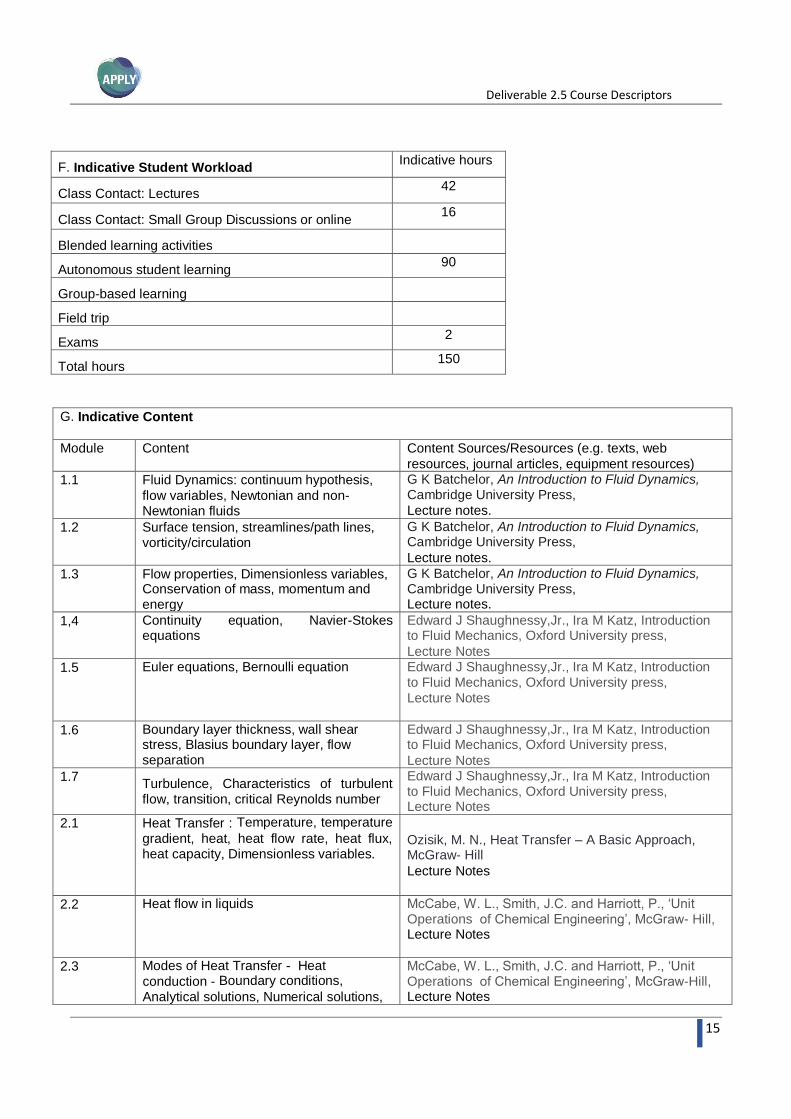
F. Indicative Student Workload Indicative hours
Class Contact: Lectures 42
Class Contact: Small Group Discussions or online 16
Blended learning activities
Autonomous student learning 90
Group-based learning
Field trip
Exams 2
Total hours 150
G. Indicative Content
Module
Content Content Sources/Resources (e.g. texts, web
resources, journal articles, equipment resources)
1.1 Fluid Dynamics: continuum hypothesis,
flow variables, Newtonian and non-Newtonian fluids
G K Batchelor, An Introduction to Fluid Dynamics, Cambridge University Press, Lecture notes.
1.2 Surface tension, streamlines/path lines, vorticity/circulation
G K Batchelor, An Introduction to Fluid Dynamics, Cambridge University Press, Lecture notes.
1.3 Flow properties, Dimensionless variables, Conservation of mass, momentum and energy
G K Batchelor, An Introduction to Fluid Dynamics, Cambridge University Press, Lecture notes.
1,4 Continuity equation, Navier-Stokes equations
Edward J Shaughnessy,Jr., Ira M Katz, Introduction to Fluid Mechanics, Oxford University press,
Lecture Notes
1.5 Euler equations, Bernoulli equation Edward J Shaughnessy,Jr., Ira M Katz, Introduction to Fluid Mechanics, Oxford University press,
Lecture Notes
1.6 Boundary layer thickness, wall shear stress, Blasius boundary layer, flow separation
Edward J Shaughnessy,Jr., Ira M Katz, Introduction to Fluid Mechanics, Oxford University press,
Lecture Notes
1.7 Turbulence, Characteristics of turbulent flow, transition, critical Reynolds number
Edward J Shaughnessy,Jr., Ira M Katz, Introduction to Fluid Mechanics, Oxford University press, Lecture Notes
2.1 Heat Transfer : Temperature, temperature
gradient, heat, heat flow rate, heat flux, heat capacity, Dimensionless variables.
Ozisik, M. N., Heat Transfer – A Basic Approach, McGraw- Hill
Lecture Notes
2.2 Heat flow in liquids McCabe, W. L., Smith, J.C. and Harriott, P., ‘Unit Operations of Chemical Engineering’, McGraw- Hill, Lecture Notes
2.3 Modes of Heat Transfer - Heat
conduction - Boundary conditions,
Analytical solutions, Numerical solutions,
McCabe, W. L., Smith, J.C. and Harriott, P., ‘Unit Operations of Chemical Engineering’, McGraw-Hill, Lecture Notes

Deliverable 2.5 Course Descriptors
16
Heat conduction in Navier-Stokes equations
2.4 Heat transfer for forced and free convection
McCabe, W. L., Smith, J.C. and Harriott, P., ‘Unit Operations of Chemical Engineering’, McGraw- Hill,
Lecture Notes
2.5 Heat radiation - Black-body radiation, radiation of real objects
Heat Transfer: A Practical Approach, McGraw‐Hill,
Lecture Notes
2.6 Heat exchange equimpment McCabe, W. L., Smith, J.C. and Harriott, P., ‘Unit Operations of Chemical Engineering’, McGraw- Hill,
Lecture Notes
2.7 Evaporation Processes McCabe, W. L., Smith, J.C. and Harriott, P., ‘Unit Operations of Chemical Engineering’, McGraw- Hill,
Lecture Notes

Deliverable 2.5 Course Descriptors
17
4. Hands-on Computational Fluid Dynamics (part 1)
Course Title: Hands-on Computational Fluid Dynamics (part 1)
Course Code: APPLY C3
Course Type: Core ☒ Elective ☐
Credits: 6 ECTS
Semester: 1
Course Coordinator: MAHE
Course Review: VIT
A. Course Description
Lectures in the course are designed to cover the terminology and core concepts and theories in CFD. To introduce the student to the basic tools of computer-aided design. The set of examples are designed to provide the student with the necessary tools for using commercial CFD software. A set of laboratory tasks will take the student through
a series of increasingly complex flow and heat transfer simulations, requiring an understanding of the basic theory of computational fluid dynamics (CFD).
B. Modules
Module name Introduction to CFD and ANSYS Workbench (CFX/FLUENT) Number 1
Total hours 22 Class hours 6 Autonomous study hours 16
Module description
The module will introduce CFD and its applications in various engineering problems, review the CFD process. The students will be familiarized with the workbench interface, various options for solving any CFD problem. Lab sessions on creating geometry and meshing; Defining a CFD problem; Familiarization with Design Modeler and
Space Claim, Creating and/or Importing 2D Geometry in Design Modeller,
Module assessment methodology
Assignment-submission of lab reports, Viva voce, Lab exam
Module name Overview of Meshing Techniques for 2D flow problems Number 2
Total hours 24 Class hours 8 Autonomous study hours 16
Module description
Meshing the 2D Geometry; workbench mesh and ICEM Mesh, Meshing Techniques, structured and Unstructured mesh, Mapped mesh, Mesh Refinement, Quality of Mesh,
Module assessment methodology
Assignment-submission of lab reports, Viva voce, Lab exam
Module name Application of CFD for incompressible flows-Jet dynamics Number 3

Deliverable 2.5 Course Descriptors
18
Total hours 24 Class hours 8 Autonomous study hours 16
Module description: Flow over an Airfoil
Modeling/import of an airfoil in design Modeller, meshing techniques, Laminar flow fundamentals, Angle of Attack, Variation of Reynolds number, lift and drag, post processing results
Module assessment methodology
Assignment-submission of lab reports, Viva voce, Lab exam
Module name Flow over an airfoil Number 4
Total hours 22 Class hours 8 Autonomous study hours 14
Module description: boundary layer Development
Basics of 3D modeling and meshing. Inflation layers, Hybrid meshing, Y+ value, Fundamentals of turbulence, comparison of turbulence models
Module assessment methodology
Assignment-submission of lab reports, Viva voce, Lab exam
Module name Flow over a cylinder Number 5
Total hours 22 Class hours 8 Autonomous study hours 14
Module description: User Defined Functions
Axisymmetric conditions, transient flow, user defined function (UDF) post processing, wake formation, animation
Module assessment methodology:
Assignment-submission of lab reports, Viva voce, Lab exam
Module name A 3D bifurcating Artery Number 6
Total hours 18 Class hours 6 Autonomous study hours 12
Module description: Incompressible and Compressible flows
Fundamentals of Incompressible and Compressible flows, nozzle design, Analysis of over expanded Nozzle and
under expanded nozzles
Module assessment methodology

Deliverable 2.5 Course Descriptors
19
Assignment-submission of lab reports, Viva voce, Lab exam
Module name Advanced aspects of post processing Number 7
Total hours 18 Class hours 6 Autonomous study hours 12
Module description: Heat Transfer
Energy equation, combustion, porous media, NOx emissions
Module assessment methodology
Assignment-submission of lab reports, Viva voce, Lab exam
C. Course Learning Outcomes. Upon completion of the course, students will be able to
1. Perform geometry modeling of simple fluid flow problems
2. Develop different types of mesh for extrapolating the basic equations of flow
3. Perform 2D analysis to understand the forces developed due to aerodynamic shape such as airfoil
4. Compare the boundary layer development for a flat plate and a simple pipe flow
5. Develop user defined functions to simulate flow over cylinder
6. Analyze the compressible flow in a Nozzle
7. Simulate the application of energy equation in combustion
Transferable Skills: - Development of 2D and 3D models for fluid flow. - Discritization of Geometry (Meshing)
- User Defined Functions - Flow visualization, animation
D. Assessment strategies
Assessment Type Percentage of Final Marks
☒ Exam (EX) 40
☐ Presentation (PRS) -
☐ Portfolio (PTO) -
☐ Multiple Choice Exam (MCQ) -
☒ Assignment (ASM) 40
☒ Design Project (DPR) 10
☐ Debate (DEB) -
☒ Lab viva voce 10

Deliverable 2.5 Course Descriptors
20
E. Assessment strategies description
Exams
A final lab exam of 2 hours duration will be conducted to assess the learning outcomes of students. Students will be asked to perform any one subcomponent of CFD simulation (geometry modeling/grid generation/solution setup/ post processing of given set of data) of a given problem.
Assignments
Students will have to complete at least one numerical experiment as the part of each module. Subsequent to the class hour teaching, students must complete the experiment in sense by spending the additional autonomous
study hours. Assessment will be done based on the merit of detailed lab report of each experiment.
Project
Students will be encouraged to take up independent CFD projects of their interest. Based on the merit of submitted
project report and presentation of results before the project evaluation committee, marks will be awarded
Viva voce
An oral examination to assess the level of knowledge gained by the students through this course. Maximum test
duration will be 15 minutes and 8-12 questions, randomly covering the course content will be asked.
F. Indicative Student Workload Indicative hours
Class Contact: Lectures 50
Class Contact: Small Group Discussions or online
Blended learning activities
Autonomous student learning 100
Group-based learning
Exams
Total hours 150
G. Reference text books
1 Ansys Fluent 2020 R1-Theory Guide
2 Versteeg, Henk Kaarle, and Weeratunge Malalasekera. An introduction to computational fluid dynamics: the finite volume method. Pearson education, 2007.
3 John Matsson, An Introduction to ANSYS Fluent 2020, SDC Publications, 2020
4 Suhas Patankar, Numerical heat transfer and fluid flow, CRC Press
5 Blazek, Jiri. Computational fluid dynamics: principles and applications. Butterworth-Heinemann, 2015.
6 John D. Anderson, Jr, Computational Fluid Dynamics: The Basics with Applications
7 Jiyuan Tu , Guan Heng Yeoh , Chaoqun Liu, Computational Fluid Dynamics: A Practical Approach, Butterworth-Heinemann 2007

Deliverable 2.5 Course Descriptors
21
H. Indicative Lab experiments
Module
Content
1 Geometry modelling: Modelling using Geometric Modeller, space claims, CATIA
2 Structured Mesh, Unstructured Mesh, Mesh export
3 Flow over an airfoil
4 Flat plate and pipe flow boundary layer comparison
5 Steady and Unsteady Flow Past a Cylinder
6 Over expanded and Under expanded Nozzle
7 Bifurcating Artery
8 Hospital ventilation-Fan boundary
9 Natural convection
10 Flow across Porous Media
11 Partially Premixed Combustion
12 Wind Turbine blade
Deliverable 2.5 Course Descriptors
22
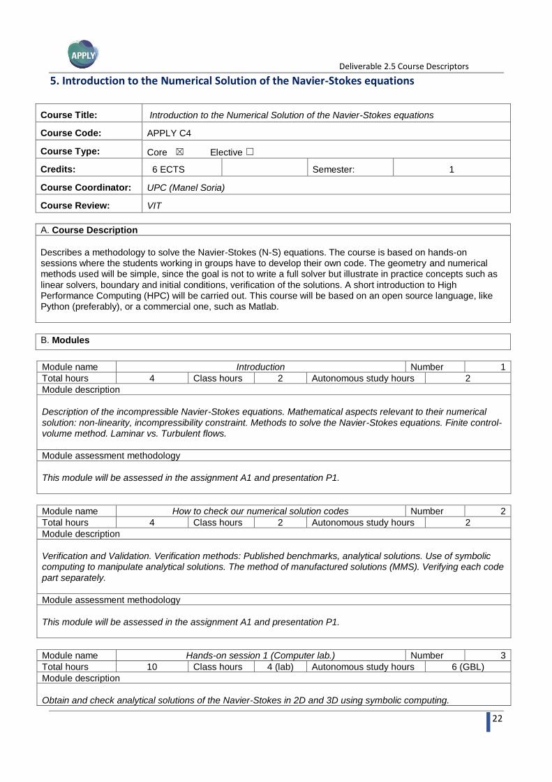
5. Introduction to the Numerical Solution of the Navier-Stokes equations
Course Title: Introduction to the Numerical Solution of the Navier-Stokes equations
Course Code: APPLY C4
Course Type: Core ☒ Elective ☐
Credits: 6 ECTS
Semester: 1
Course Coordinator: UPC (Manel Soria)
Course Review: VIT
A. Course Description
Describes a methodology to solve the Navier-Stokes (N-S) equations. The course is based on hands-on sessions where the students working in groups have to develop their own code. The geometry and numerical methods used will be simple, since the goal is not to write a full solver but illustrate in practice concepts such as
linear solvers, boundary and initial conditions, verification of the solutions. A short introduction to High Performance Computing (HPC) will be carried out. This course will be based on an open source language, like Python (preferably), or a commercial one, such as Matlab.
B. Modules
Module name Introduction Number 1
Total hours 4 Class hours 2 Autonomous study hours 2
Module description
Description of the incompressible Navier-Stokes equations. Mathematical aspects relevant to their numerical
solution: non-linearity, incompressibility constraint. Methods to solve the Navier-Stokes equations. Finite control-volume method. Laminar vs. Turbulent flows.
Module assessment methodology
This module will be assessed in the assignment A1 and presentation P1.
Module name How to check our numerical solution codes Number 2
Total hours 4 Class hours 2 Autonomous study hours 2
Module description
Verification and Validation. Verification methods: Published benchmarks, analytical solutions. Use of symbolic computing to manipulate analytical solutions. The method of manufactured solutions (MMS). Verifying each code
part separately.
Module assessment methodology
This module will be assessed in the assignment A1 and presentation P1.
Module name Hands-on session 1 (Computer lab.) Number 3
Total hours 10 Class hours 4 (lab) Autonomous study hours 6 (GBL)
Module description
Obtain and check analytical solutions of the Navier-Stokes in 2D and 3D using symbolic computing.

Deliverable 2.5 Course Descriptors
23
Module assessment methodology
This module will be assessed in the assignment A1 and presentation P1.
Module name Starting our code Number 4
Total hours 4 Class hours 2 Autonomous study hours 2
Module description
Scope of the first code. Use of staggered meshes. Understanding the mesh disposition. Description of the mesh. Halo update function. Print field function. Numerical representations of analytic distributions. Guidelines to write
good code: modularity, quality of the documentation.
Module assessment methodology
This module will be assessed in the assignment A1 and presentation P1.
Module name Hands-on session 2 (Computer lab.) Number 5
Total hours 12 Class hours 4 (lab) Autonomous study hours 8 (GBL)
Module description
Writing and testing the initial Navier-Stokes solver functions.
Module assessment methodology
This module will be assessed in the assignment A1 and presentation P1.
Module name Discretization of diffusive and convective terms Number 6
Total hours 8 Class hours 4 Autonomous study hours 4
Module description
Expressing diffusive and convective terms as a divergence. Discretization of diffusive term. Discretization of convective term. Numerical scheme. Kinetic-energy preserving discretization. Upwind scheme. Verification.
Module assessment methodology
This module will be assessed in the assignment A1 and presentation P1.
Module name Hands-on session 3 (Computer lab.) Number 7
Total hours 16 Class hours 4 (lab) Autonomous study hours 12 (GBL)
Module description
Writing and testing functions for the diffusive and convective terms.
Module assessment methodology
This module will be assessed in the assignment A1 and presentation P1.
Module name Presentation of results - P1 Number 8
Total hours 6 Class hours 2 Autonomous study hours 4
Module description

Deliverable 2.5 Course Descriptors
24
Each group will present its work to the class and answer the questions of the other groups and the professor
Module assessment methodology
-
Module name Time marching algorithm and the incompressibility constraint Number 9
Total hours 4 Class hours 2 Autonomous study hours 2
Module description
Understanding the problem of pressure-velocity coupling. Ladyzhenskaya theorem. Velocity/pressure coupling and time integration. The predictor velocity. Recovering the pressure.
Module assessment methodology
This module will be assessed in the assignment A2 and presentation P2.
Module name Pressure-velocity coupling and the Poisson equation Number 10
Total hours 10 Class hours 4 Autonomous study hours 6
Module description
Obtaining the discrete Poisson equation. Avoiding the singularity. Compatibility. Physical interpretation of the compatibility condition. Physical interpretation of the singularity. Interpretation of the pressure values obtained. Solving the Poisson equation in real applications. Computational complexity of an algorithm. Role and limitations
of parallel computers. Field representations and algebraic representations. The divergence and gradient functions..
Module assessment methodology
This module will be assessed in the assignment A2 and presentation P2.
Module name Hands-on session 4 (Computer lab.) Number 11
Total hours 14 Class hours 4 (lab) Autonomous study hours 10 (GBL)
Module description
Writing and testing functions for pressure-velocity coupling.
Module assessment methodology
This module will be assessed in the assignment A2 and presentation P2.
Module name Hands-on session 5 (Computer lab.) Number 12
Total hours 26 Class hours 6 (lab) Autonomous study hours 20 (GBL)
Module description
Finishing and verifying our first Navier-Stokes solver.
Testing different numerical schemes.
Module assessment methodology
This module will be assessed in the assignment A2 and presentation P2.

Deliverable 2.5 Course Descriptors
25
Module name Boundary conditions Number 13
Total hours 8 Class hours 4 Autonomous study hours 4
Module description
Dirichlet condition (value). Neumann condition (derivative). Effects on our code. How to implement them. Boundary conditions with effect on the compressibility constraint: Inlets and outlets.
Using benchmark solutions: the driven-cavity problem.
Module assessment methodology
This module will be assessed in the assignment A3 and presentation P2.
Module name Hands-on session 6 (Computer lab.) Number 13
Total hours 18 Class hours 4 (lab) Autonomous study hours 14 (GBL)
Module description
Implementing the driven-cavity problem.
Module assessment methodology
This module will be assessed in the assignment A3 and P2.
Module name Presentation of the results – P2 Number 14
Total hours 6 Class hours 2 Autonomous study hours 4
Module description
Each group will present its work to the class and answer the questions of the other groups and the professor.
Module assessment methodology
-
C. Course Learning Outcomes. Upon completion of the course, students will be able to
1. Understand symbolic computing and its utility to manipulate long algebraic expressions.
2. Understand the numerical problems associated with the Navier-Stokes equations
3. Know several techniques to validate PDE solvers
4. Know and apply guidelines to write good scientific / engineering software
5. Understand finite-control volume method for incompressible Navier-Stokes equations
6. Understand the problem of pressure-velocity coupling in the incompressible Navier-Stokes equations
7. Know how to implement several basic boundary conditions to the incompressible Navier-Stokes equations
Transferable Skills: - Code development and verification. - Symbolic computing.
- Understanding boundary conditions and how to implement them. - Understanding Navier-Stokes equations.

Deliverable 2.5 Course Descriptors
26
D. Assessment strategies
Assessment Type Percentage of Final Marks
☐ Exam (EX) -
☒ Presentation (PRS) 40
☐ Portfolio (PTO) -
☐ Multiple Choice Exam (MCQ) -
☒ Assignment (ASM) 60
☐ Design Project (DPR) -
☐ Debate (DEB) -
E. Assessment strategies description
Assignments
The students will be requested to deliver 3 assignments, each of them will be 20% of the final mark.
A1. Implement and validate convective and diffusive terms. A2. Implement and validate a Navier-Stokes solver with periodic boundary conditions. A3. Final Navier-Stokes solver.
Presentation
There will be two presentations: P1. Implement and validate convective and diffusive terms. (20% of the final mark) P2. Final Navier-Stokes solver (test with analytic functions and driven cavity). (20% of the final mark)
Each group will present its work to the class and answer the questions of the other groups and the professor.
F. Indicative Student Workload Indicative hours
Class Contact: Lectures 20
Class Contact: Small Group Discussions or online
Computer laboratory sessions 26
Blended learning activities
Autonomous student learning 30
Group-based learning 70
Field trip
Exams (presentations) 4
Total hours 150

Deliverable 2.5 Course Descriptors
27
G. Indicative Content
Module
Content Content Sources/Resources (e.g. texts, web
resources, journal articles, equipment resources)
1 Introduction
PowerPoints / PDFs , Lecture notes,
A personal computer with a programing environment. Anderson , J. “Computational Fluid Dynamics”,
McGraw-Hill
Versteeg, H. “An Introduction to Computational Fluid Dynamics: The Finite Volume Method”, Pearson
2 How to check our numerical solution
codes
3 Hands-on session 1
4 Starting our code
5 Hands-on session 2
6 Discretization of diffusive and convective terms
7 Hands-on session 3
8 Presentation of results
9 Time marching algorithm and the incompressibility constraint
10 Pressure-velocity coupling and the Poisson equation
11 Hands-on session 4
12 Hands-on session 5
13 Boundary conditions
14 Hands-on session 6
Additional information
The students will need to use a personal computer with a programming environment. Some examples will be in
Matlab and others in Python. While the course stresses the importance of good programming practices, it is not a
programming course. The students are assumed to have some previous knowledge and experience about
programming and maintaining small codes.

Deliverable 2.5 Course Descriptors
28
6. Turbulence modelling and simulation
Course Title: Turbulence modelling and simulation
Course Code: APPLY C5
Course Type: Core ☒ Elective ☐
Credits: 6 ECTS
Semester: 2
Course Coordinator: UPC (Ivette Rodríguez)
Course Review: UiTM
A. Course Description
This course provides the student with a background on turbulence, the concepts and tools needed to understand the physics behind turbulent flows. The course is divided into two main parts: the first half of the course introduces the student into the theoretical subjects about turbulence, turbulence scales, transport equations, etc. In the second half of the course, an overview of the different numerical modelling techniques, together with their capabilities and limitations for treating turbulent flows are presented. From Direct numerical simulations (DNS), large eddy simulations (LES) and Reynolds-averaged Navier-Stokes (RANS) equation modelling.
B. Modules
Module name Introduction Number 1
Total hours 12 Class hours 4 Autonomous study hours 8
Module description
Introduction to turbulence. The nature of turbulent flows. Scales of turbulence, can we solve them? Turbulence and its complexity, the multi-scale problem. The Navier-Stokes equations. The energy equation.
Module assessment methodology
This module will be assessed in the assignments A1 & A2 and presentation P1.
Module name Turbulent flow statistics. Number 2
Total hours 8 Class hours 2 Autonomous study hours 6
Module description
Random nature of turbulence. Turbulence length scales. Energy cascade and Kolmogorov hypothesis. Energy
spectrum.
Module assessment methodology
This module will be assessed in the assignments A1 & A2 and presentation P1.

Deliverable 2.5 Course Descriptors
29
Module name Turbulent flow statistics. Practical session (Computer lab.) Number 3
Total hours 10 Class hours 2 (lab) Autonomous study hours 8 (GBL)
Module description
From a set of numerical probes, obtain flow statistics, two-point correlations, energy spectrum, Taylor microscale. The student will write a small computer program to do this
Module assessment methodology
This module will be assessed in the assignments A1 & A2 and presentation P1.
Module name Turbulent mean flow Number 4
Total hours 12 Class hours 4 Autonomous study hours 4
Module description
Reynolds decomposition. Time average N.S equations. Reynolds stresses. The closure problem. Turbulent
transport of heat.
Module assessment methodology
This module will be assessed in the assignments A1 & A2 and presentation P1.
Module name Turbulent mean flow. Practical session (Computer lab.) Number 5
Total hours 14 Class hours 4 (lab) Autonomous study hours 10 (GBL)
Module description
Using data from a DNS, the student will write a small code to post-process the data and obtain the mean flow field and its statistics. Then, results will be analysed and compared with reference data
Module assessment methodology
This module will be assessed in the assignments A1 & A2 and presentation P1.
Module name Transport equations for kinetic energy and Reynolds stresses Number 6
Total hours 6 Class hours 2 Autonomous study hours 4
Module description
Transport equations for turbulent kinetic energy. Dissipation, production, convection and turbulent diffusion.
Reynolds stresses transport equations.
Module assessment methodology
This module will be assessed in the assignments A1 & A2 and presentation P1.
Module name Transport equations for kinetic energy and Reynolds stresses.
Practical session (Computer lab.)
Number 7
Total hours 14 Class hours 4 (lab) Autonomous study hours 10(GBL)
Module description
Using data from a DNS database, the student will write a small computer program to evaluate the turbulent kinetic energy budget.

Deliverable 2.5 Course Descriptors
30
Module assessment methodology
This module will be assessed in the assignments A1 & A2 and presentation P1.
Module name Presentation of results of assignment 1 & 2 - P1 Number 8
Total hours 6 Class hours 2 Autonomous study hours 4
Module description
Each group will present its work to the class and answer the questions of the other groups and the professor
Module assessment methodology
Module name Turbulence modelling and simulation. Introduction. Number 9
Total hours 6 Class hours 2 Autonomous study hours 4
Module description
The challenge to be faced in the simulation of turbulent flows. The wall problem. Overview of the different approaches to deal with the resolution of turbulent flows. Examples.
Module assessment methodology
This module will be assessed in the assignment A3 and presentation P2.
Module name Assessing mesh resolution. Practical session (Computer lab.) Number 10
Total hours 8 Class hours 2 (lab) Autonomous study hours 6 (GBL)
Module description
The student will write a small computer program to analyse the data from a DNS or LES in order to compute dissipation and assess mesh resolution for the approach used.
Module assessment methodology
This module will be assessed in the assignment A3 and presentation P2.
Module name Turbulence modelling. Large-eddy simulation Number 11
Total hours 8 Class hours 4 Autonomous study hours 4
Module description
Scale separation and filtering. Deriving the LES equations. SGS models. Smagorinsky and mixing length
models. Other closures. The wall problem. Resolution requirements.
Module assessment methodology
This module will be assessed in the assignment A3 and presentation P2.
Module name Large-eddy simulations. Practical session (Computer lab.) Number 12
Total hours 16 Class hours 6(lab) Autonomous study hours 10 (GBL)

Deliverable 2.5 Course Descriptors
31
Module description
Practical lesson includes the resolution with OpenFoam of a square cylinder. Results will be analysed and compared with those of the literature.
Module assessment methodology
This module will be assessed in the assignment A3 and presentation P2.
Module name Turbulence modelling. Reynolds-Averaged Navier-Stokes (RANS) models
Number 13
Total hours 10 Class hours 4 Autonomous study hours 6
Module description
Overview. Boussinesq hypothesis and eddy viscosity models. The k-ε model. Reynolds stress transport model.
Targeting industrial flows with RANS models. Limitations of RANS models.
Module assessment methodology
This module will be assessed in the assignment A3 and presentation P2.
Module name RANS models. Practical session (Computer lab.) Number 14
Total hours 18 Class hours 6(lab) Autonomous study hours 12 (GBL)
Module description
Practical lessons include the resolution of a case in OpenFoam The comparison of different RANS models and
with results of LES/DNS given to the student will give an insight into the main strengths and limitations of RANS models
Module assessment methodology
This module will be assessed in the assignment A3 and presentation P2.
Module name Presentation of the results of assignment 3– P2 Number 15
Total hours 6 Class hours 2 Autonomous study hours 4
Module description
Each group will present its work to the class and answer the questions of the other groups and the professor.
Module assessment methodology
C. Course Learning Outcomes. Upon completion of the course, students will be able to
1. Understand the physics of viscous flows,
2. Understand the physics of flow instability and laminar-turbulent transition,

Deliverable 2.5 Course Descriptors
32
3. Understand the development of the governing conservation equations problems for solving turbulent flows,
4. Understand the different levels of modelling turbulent flows,
5. Understand statistical analysis of turbulence and the general properties of turbulent shear flows,
6.. Understand the quantitative description of turbulent wall-bounded flows and to be able to calculate flow
statistics, etc.
Transferable Skills: - Understanding Navier-Stokes equations
- Understanding the different approaches to deal with turbulent flows - Mesh assessment - numerical solution verification and validation
D. Assessment strategies
Assessment Type Percentage of Final Marks
☐ Exam (EX) -
☒ Presentation (PRS) 40
☐ Portfolio (PTO) -
☐ Multiple Choice Exam (MCQ) -
☒ Assignment (ASM) 60
☐ Design Project (DPR) -
☐ Debate (DEB) -
E. Assessment strategies description
Assignments
The students will be requested to deliver 3 assignments. Assignment 1 and 2 will represent a 15 % of the final mark whereas assignment 3 weight is 30 % of the final mark.
A1: Evaluate turbulence statistics from time resolved DNS data and comparison with the literature. A2: Following A1, evaluate turbulent kinetic energy and Reynolds-stress budgets. A3: Solve a turbulent flow at high Reynolds number using different RANS models and comparison with results
from the literature.
Presentation
There will be two presentations: P1. Students will present and discuss the results obtained in A1 & A2 (20% of the final mark)
P2. Students will present and discuss results obtained in A3 (20% of the final mark) Each group will present its work to the class and answer the questions of the other groups and the professor.
F. Indicative Student Workload Indicative hours
Class Contact: Lectures 22
Class Contact: Small Group Discussions or online

Deliverable 2.5 Course Descriptors
33
Computer laboratory sessions 24
Blended learning activities
Autonomous student learning 44
Group-based learning 56
Field trip
Exams (presentations) 4
Total hours 150
G. Indicative Content
Module
Content Content Sources/Resources (e.g. texts, web resources, journal articles, equipment resources)
1 Introduction Bradshaw, P. (1971) An introduction to turbulence and its measurements. Pergamon Press
Tennekes, H. and Lumley, J. L. (1972) ‘A first course in turbulence’. MIT Press.
Pope, S. B. (2001) Turbulent Flows. Cambridge University Press.
2 Turbulent flow statistics
3 Turbulent flow statistics. Practical session
4 Turbulent mean flow
5 Turbulent mean flow. Practical session
6 Transport equations for kinetic energy and Reynolds stresses
7 Transport equations for kinetic energy and Reynolds stresses. Practical session
8 Presentation of results
9 Turbulence modelling and simulation. Introduction.
10 Assessing mesh resolution
11 Turbulence modelling. Large-eddy simulation
12 Large-eddy simulations. Practical session
13 Turbulence modelling. Reynolds-Averaged Navier-Stokes (RANS) models
14 RANS models. Practical session
15 Presentation of the results
Additional information
The students will need to use a personal computer with a programming environment. Some skills using some programming language might be advisable. Matlab or python might be used in some examples in class.
For the assignments students will need to have some type of visualisation software, Paraview might be used (it is available for all OS). For some assignments the students will need to plot their results, python,matlab/gnuplot or other graphing software might be used. For some practical lessons and the last assessment OpenFoam will be
used. The student will need to install this CFD software into their personal computer. The students are assumed to have some previous knowledge and experience about programming and maintaining small codes

Deliverable 2.5 Course Descriptors
34
7. Hands-on Computational Fluid Dynamics (part 2)
Course Title: Hands-on Computational Fluid Dynamics (part 2)
Course Code: APPLY C6
Course Type: Core ☒ Elective ☐
Credits: 6 ECTS
Semester: 2
Course Coordinator: VIT
Course Review: MAHE
A. Course Description
This course enables students to apply CFD methods for the design and analysis of engineering systems involving fluid flow and heat transfer. The course covers advanced topics which include preprocessing, solution setup and post processing procedures of CFD. The first two modules of this course provide detailed grid generation methods,
including structured and unstructured approaches. Both commercial and open source CAD and grid generation packages will be used to provide hands on-experience to the students. The next four modules are then framed to introduce solver setup for executing specific flow problems chosen from many fields of applications - aerospace,
automotive, turbo machinery, multi-phase flow etc. The last module of this course aims to familiarize the student with post processing and visualization tools. This lab based course will train the students through the execution of 10 different experiments-2 based on grid generation, 6 based on flow problems and 2 based on post processing.
B. Modules
Module name Advanced aspects of CAD modeling and surface meshing Number 1
Total hours 18 Class hours 6 Autonomous study hours 12
Module description
Review of basics of geometry modeling-Geometry handling and CAD repairing-Domain Decomposition with Multi-Blocking-Remarks on Block Topology For Multi-Block Meshing-Hybrid Blocking- Unstructured and Multi-
Zone meshing methods-surface meshing, Structured blocking and meshing for 2D flow problems-Local grid refinement-boundary layer meshing- Demonstration of Cartesian grid schemes over 2D domains-Adaptive grid refinement, Immersed Boundary Methods, Cut Cell based Methods, Chimera Grid Schemes.
Module assessment methodology
Assignment-submission of lab reports, Viva voce, Lab exam
Module name Guidelines on grid generation-complex 3D flow problems Number 2
Total hours 20 Class hours 8 Autonomous study hours 12
Module description
Automatic generation of Unstructured Meshes, Multi-Block Mesh Generation, importance of grid topology, Generation of orthogonal hexahedral elements for cylindrical objects like internal combustion engine cylinder through O grid. Creation of hexahedral C-Grid for piston bowl and L- grid meshes using blocking methodologies.
Generation of tetrahedral mesh for complex geometry using Octree algorithm. Development of prism layers over tetrahedral elements for capturing rotor stator interfaces of turbo machinery components. grid quality and grid design, local refinement and grid adaptation, Definitions of Size Functions - Mesh Sensitivity and Mesh
Independence Study- Mesh editing, smoothening or quality improvement.

Deliverable 2.5 Course Descriptors
35
Module assessment methodology
Assignment-submission of lab reports, Viva voce, Lab exam.
Module name Application of CFD for incompressible flows-Jet dynamics Number 3
Total hours 20 Class hours 8 Autonomous study hours 12
Module description
Review of Solution of Navier-Stokes Equations governing incompressible flow using FVM-Pressure based solvers, Pressure-velocity coupling Techniques, Laminar vs Turbulent flows, Features and applications of jet, Jet
flow analysis using RANS and LES approach, Boundary conditions, Selection of Numerical schemes, Defining the required fluid properties, solver setup for steady and transient flow analysis, Confirmation of convergence, Transient data collection.
Module assessment methodology
Assignment-submission of lab reports, Viva voce, Lab exam.
Module name Application of CFD for compressible flows-Aerodynamics Number 4
Total hours 20 Class hours 8 Autonomous study hours 12
Module description
Review of governing equations for compressible flows-Subsonic, transonic and supersonic flows-density based
solvers, Requirement of solution of energy equation, Internal and external flow aerodynamics-cascade flows, shock waves, shock capturing, shock-shock and shock wave-boundary layer interactions, Solution of inviscid, laminar and turbulent flows. Steady and transient flow analysis, boundary conditions, implicit and explicit
algorithms, CFL criterion, solution steering, higher order accuracy in spatial and temporal discretization, use of gas models, fixing of convergence criteria/simulation time, Methods of solution validation.
Module assessment methodology
Assignment-submission of lab reports, Viva voce, Lab exam.
Module name Application of CFD for Multiphase flow analysis Number 5
Total hours 20 Class hours 8 Autonomous study hours 12
Module description
Introduction to multiphase flow, types and applications, Common terminologies, flow patterns and flow pattern maps, Homogeneous and separated flow Analysis, Modelling: Solid - Liquid, Liquid - Liquid, Gas - Liquid two
phase flow Analysis using VOF and DPM models, Boiling and Non-Boiling flow, Validation of simulated results using basic measurement techniques for multiphase flows.
Module assessment methodology
Assignment-submission of lab reports, Viva voce, Lab exam.
Module name Application of CFD for Fluid-Structure Interaction (FSI) analysis Number 6
Total hours 18 Class hours 6 Autonomous study hours 12
Module description

Deliverable 2.5 Course Descriptors
36
Review of FSI-Introduction to FSI , Significance of FSI, Governing Equations of Fluid and Structural Mechanics, Theoretical aspects of Fluid-Structure Interactions - i) Potential Flow (Inertial Coupling) ii) Viscous Flow (Viscous
Damping) iii) Compressible Flow (Radiation Damping). Formulation of Arbitrary Lagrangian-Eulerian (ALE) and Space-time methods. Numerical aspects of Fluid-Structure Interactions - Finite Element and Boundary Element Methods – Different types of interface boundary conditions - Types of FSI – One way transfer and two way
transfer. Applications of FSI - Hands on Numerical experiment with FSI .
Module assessment methodology
Assignment-submission of lab reports, Viva voce, Lab exam.
Module name Advanced aspects of post processing Number 7
Total hours 18 Class hours 6 Autonomous study hours 12
Module description
Script writing for large data processing; Gradient , Vector and Tensor Calculations of flow properties; Identification of different zone using Velocity and pressure distribution; Turbulence measurements, Reynolds shear stress distribution, Budget of turbulent kinetic energy, creation of numerical schlieren images, Evolution of
the momentum flux, Identification of fluid structures using Q-function, Lambda2-function, Coherent structures, Estimation of turbulent length scales.
Module assessment methodology
Assignment-submission of lab reports, Viva voce, Lab exam.
C. Course Learning Outcomes. Upon completion of the course, students will be able to
1. Perform geometry modeling of complex domains
2. Create grids required for simulating complex flow structures
3. Setup and execute incompressible flow simulations
4. Setup and execute compressible flow simulations
5. Simulate simple multiphase flows by choosing suitable multiphase flow models
6. Setup and execute Fluid structure interaction simulations
7. Perform post processing of data obtained from the simulations and visualize/represent the results in an appropriate manner.
Transferable Skills: - Geometry modeling. - Grid generation.
- Effective use of solvers suited to a particular problem - Post processing and result analysis
D. Assessment strategies
Assessment Type Percentage of Final Marks
☒ Exam (EX) 40
☐ Presentation (PRS) -

Deliverable 2.5 Course Descriptors
37
☐ Portfolio (PTO) -
☐ Multiple Choice Exam (MCQ) -
☒ Assignment (ASM) 40
☒ Design Project (DPR) 10
☐ Debate (DEB) -
☒ Lab viva voce 10
E. Assessment strategies description
Exams
A final lab exam of 2 hours duration will be conducted to assess the learning outcomes of students. Students will
be asked to perform any one subcomponent of CFD simulation (geometry modeling/grid generation/solution setup/ post processing of given set of data) of a given problem.
Assignments
Students will have to complete at least one numerical experiment as the part of each module. Subsequent to the
class hour teaching, students must complete the experiment by utilizing the allotted additional autonomous study hours. Assessment will be done based on the merit of detailed lab report of each experiment.
Project
Students will be encouraged to take up independent CFD projects of their interest. Based on the merit of submitted
project report and presentation of results before the project evaluation committee, marks will be awarded.
Viva voce
An oral examination to assess the level of knowledge gained by the students through this course. Maximum test duration will be 15 minutes and 8-12 questions, randomly covering the course content will be asked.
F. Indicative Student Workload Indicative hours
Class Contact: Lectures 50
Class Contact: Small Group Discussions or online
Blended learning activities
Autonomous student learning 84
Exams

Deliverable 2.5 Course Descriptors
38
Total hours 134
G. Reference text books
1 Edelsbrunner, Herbert. Geometry and topology for mesh generation. Cambridge University Press, 2001.
2 Sadrehaghighi, Ideen. "Mesh generation in CFD." CFD Open Ser 151 (2017).
3 Tu, Jiyuan, Guan Heng Yeoh, and Chaoqun Liu. Computational fluid dynamics: a practical approach. Butterworth-Heinemann, 2018.
4 Versteeg, Henk Kaarle, and Weeratunge Malalasekera. An introduction to computational fluid dynamics: the finite volume method. Pearson education, 2007.
5 Blazek, Jiri. Computational fluid dynamics: principles and applications. Butterworth-Heinemann, 2015.
6 Moukalled, Fadl, L. Mangani, and Marwan Darwish. The finite volume method in computational fluid dynamics-. An Advanced Introduction with OpenFOAM® and Matlab® Vol. 113. Berlin, Germany:: Springer, 2016.
7 Yeoh, Guan Heng, and Jiyuan Tu. Computational techniques for multiphase flows. Butterworth-Heinemann, 2019.
8 Bazilevs, Yuri, Kenji Takizawa, and Tayfun E. Tezduyar. Computational fluid-structure interaction: methods and applications. John Wiley & Sons, 2013.
9 Ansys Fluent 2020 R1-Theory Guide
H. Indicative Lab experiments
Sl. No.
Title
1 Geometry modelling: Multi-Blocking of a Wing-Fuselage Geometry
2 2D Grid generation for the simulation of turbulent flow over a flat plate
3 3D Multi-block grid generation for the simulation of flow over a passenger car
4 Simulation of turbulent jet impinging on a flat surface
5 Simulation of shell and tube heat exchanger
6 Simulation of transonic flow in a NGV cascade
7 Simulation of 2D and 3D supersonic flow over a bump in a channel
8 Simulation of shock wave-boundary layer interaction in hypersonic flows
9 Numerical prediction of flow patterns of liquid-liquid pipe flows
10 Numerical study of wet-steam flow in Moore nozzles
11 FSI study of Flow Past an Elastic Beam Attached to a Fixed, Rigid Block
12 3D flowfield analysis of a vertical axis wind turbine using moving reference frame (MRF)
12 Post processing for the visualisation of numerical schlieren images of complex shock trains in a supersonic air intake.
13 Scripting for the identification of fluid structures using Q-function and Lambda2-function

Deliverable 2.5 Course Descriptors
39
8. Computational Aerodynamics
Course Title: Computational Aerodynamics
Course Code: APPLY E1
Course Type: Core ☐ Elective ☒
Credits: 6 ECTS
Semester: 2
Course Coordinator: CMU (Watchapon Rojanaratanangkule)
Course Review: NU/VIT
A. Course Description
Give an insight on the simulation of external flows that are pivotal in the design of vehicles and are an integral part of R&D in the aerospace and automotive industries. This course will cover a wide range of external flow problems and provide an introduction to the CFD methods used for their simulation. It will discuss the factors that affect the accuracy of the simulations, depending on the flow characteristics, in subsonic, supersonic and hypersonic regimes and demonstrate the most appropriate techniques and CFD methods for each kind of flow.
B. Modules
Module name Fundamental of aerodynamics Number 1
Total hours 45 Class hours 15 Autonomous study hours 30
Module description
- Review of 1D gasdynamics and basic concept from thermodynamics. - Two-dimensional gas dynamics (Oblique shock waves; shock reflections (regular and Mach);
shock/shock interactions; Prandtl-Meyer expansion waves; shock/expansion method for airfoils;
under/over-expanded flow; supersonic wind tunnel.) - Conservation laws and simplifications (Conservation of mass, momentum and energy leading to the
compressible Navier–Stokes equations. Euler and potential flow equations.)
- External aerodynamics (Flow patterns in transonic and supersonic airfoil flow; critical Mach number; thin airfoils in compressible flow; velocity potential and pressure coefficient).
Module assessment methodology
Exam: Theory of aerodynamics.
Module name Introduction to CFD Number 2
Total hours 30 Class/Lab
hours
9 Autonomous study hours 21
Module description
- Governing equations and boundary conditions. - Review of basic numerical methods: finite differences, finite elements, and finite volumes. - Stability and convergence.
- Pre-processing: Geometry and grids. Grid quality. - Introduction to CFD open source software (e.g. OpenFOAM, SU2 code, PyFR, etc.). -
Module assessment methodology
Exam: CFD theory.

Deliverable 2.5 Course Descriptors
40
Module name Simulation of inviscid flows Number 3
Total hours 24 Class/Lab
hours
6 Autonomous study hours 18
Module description
- Review of governing equations of inviscid flows. - Treatment of shocks: artificial viscosity, Riemann solvers. Boundary conditions. - 1D and 2D inviscid test cases (e.g. shock tube, double Mach reflection, etc.)
Module assessment methodology
Assignment: 1D/2D simulation of shock wave.
Module name Simulation of viscous flows and introduction to turbulence modelling.
Number 4
Total hours 24 Class/Lab hours
6 Autonomous study hours 18
Module description
- Viscous effects.
- Review of boundary layers: laminar, transition and turbulent boundary layers. - Introduction to turbulence simulation: RANS, LES, DES, DNS. - Simulations of flows about aerodynamic shapes such as aerofoils.
Module assessment methodology
Assignment: 2D/3D simulation of aerofoil, wing or aircraft at relatively high Reynolds number.
Module name Aerodynamics case studies Number 5
Total hours 66 Lab hours 9 Autonomous study hours 57
Module description
- Various examples of simulations of aerodynamics applications.
Module assessment methodology
Individual project about simulation of aerodynamics applications using open source software.

Deliverable 2.5 Course Descriptors
41
C. Course Learning Outcomes. Upon completion of the course, students will be able to
1. Understand the basic principles for the computational aerodynamic analysis and design of aeronautical configurations, their limitations and range of applicability.
2. Utilize open-source CFD codes to perform flow simulations about aerodynamics applications (e.g.
shockwave, aerofoils, etc.), interpret the results and be able to quantify the errors.
Transferable Skills:
- Ability to work of software-related projects.
D. Assessment strategies
Assessment Type Percentage of Final Marks
Exam (EX) 40
Presentation (PRS) -
☐ Portfolio (PTO) -
☐ Multiple Choice Exam (MCQ) -
Assignment (ASM) 30
Design Project (DPR) 30
☐ Debate (DEB) -
E. Assessment strategies description
Exams
This course will have 1 exam, 2 months after the beginning of the course, with a 40% of the final mark weight. The exams will have 2 parts: theories of aerodynamics (30%) and CFD (10%).
Assignments
The students will be requested to deliver 2 assignments. Each weight is 15% of the final mark. Assignment 1: 1D/2D simulation of shock wave. It will reflect the knowledge obtained during the Module 3. Assignment 2: 2D/3D simulation of aerofoil, wing or aircraft at relatively high Reynolds number.
Project
A term project is assigned to the students during the beginning of the 5 th module. Student must choose their own topic related to simulation of aerodynamics applications. The simulation must be done using an open source software.
F. Indicative Student Workload Indicative hours
Class Contact: Lectures 27
Class Contact: Small Group Discussions or online -
Computer Laboratory Sessions 18
Blended learning activities -

Deliverable 2.5 Course Descriptors
42
Autonomous student learning 144
Group-based learning
Field trip
Exams 3
Total hours 150
G. Indicative Content
Module
Content Content Sources/Resources (e.g. texts, web resources, journal articles, equipment resources)
1 Fundamental of aerodynamics (Exam 1: 30)
PowerPoint, video lecture, PDF lecture notes,journal article,
Text books:
- Applied computational aerodynamics : a modern engineering approach, Russell M.
Cummings, William H. Mason, Scott A. Morton, and David R. McDaniel, 2015 by Cambridge University Press.
2 Introduction to CFD: Governing equations and boundary conditions. Review of basic numerical methods: finite differences, finite elements, and finite volumes. Stability and convergence. (Exam 2: 10)
3 Simulation of inviscid flows. Treatment of shocks: artificial viscosity, Riemann solvers. Boundary conditions. (Assignment 1: 15)
4 Simulation of viscous flows and introduction to turbulence modelling. (Assignment 2: 15)
5 Aerodynamics case studies. Projects (30)

Deliverable 2.5 Course Descriptors
43
9. Chemically Reacting Flows – Combustion
Course Title: Chemically Reacting Flows - Combustion (Energy, A&T)
Course Code: APPLY E2
Course Type: Core ☐ Elective ☒
Credits: 6 ECTS
Semester: 1
Course Coordinator: UCr
Course Review: MUJ
A. Course Description
The module introduces theory and methodology to simulate reacting flows with CFD. Various approaches of
incorporating species transport and coupling the interaction between turbulence and chemistry will be covered. Multi-phase spray modelling will be briefly introduced. Examples of combustion simulations in typical gas turbine combustors will be provided to student via a set of tutorials. Commercial CFD codes ANSYS FLUENT will be
used.
B. Modules
Module name Introduction to combustion flow physics Number 1
Total hours 15 Class hours 4 Autonomous study hours 8
Module description
Introduction to flame types, categorized as premixed/diffusion flame, laminar and turbulent flame, lean and rich combustion and their corresponding applications. Introduction to the physics of turbulence-chemistry interaction and different flame regimes and to the importance of turbulence models (RANS and LES).
Module assessment methodology
Exam and assignment
Module name Reacting flow numerical modelling methods Number 2
Total hours 30 Class hours 8 Autonomous study hours 16
Module description
Introduction to various combustion and turbulence-chemistry interaction models. Concept of reaction
mechanism, reaction rate, flamelet and PDF models. Basic governing equations for enthalpy and species transport.
Module assessment methodology
Exam and assignment
Module name Application of reacting flow for gas turbine combustors Number 3
Total hours 45 Class hours 15 Autonomous study hours 30
Module description

Deliverable 2.5 Course Descriptors
44
Combustion simulation of a gas turbine combustor. Geometry import, meshing, model selection, boundary condition setup, simulation and post-processing.
Module assessment methodology
Submit assignment on generic gas turbine combustion case analysis.
Module name Introduction to spray modelling Number 4
Total hours 18 Class hours 5 Autonomous study hours 10
Module description
Introduction of fuel injection modelling methods commonly used: Lagrangian model and Eulerian model. The focus will be the Discrete Phase Modelling technique (Lagrangian model). Basics of modelling continuous and discrete phases simultaneously will be covered, including governing equations, solver
methodology and best practices.
Module assessment methodology
Exam, assignment
Module name Spray modelling application Number 5
Total hours 22 Class hours 8 Autonomous study hours 16
Module description
A tutorial on demonstrating steps for modelling fuel injection of a generic atomiser using Discrete Phase
Modelling method, including mesh generation, model selection, boundary condition setup, solver setup and post-processing.
Module assessment methodology
Submission of assignment on simulating and analysing the fuel droplet characteristics of a generic
atomizer.
Module name Combustion simulation with liquid fuel atomisation Number 5
Total hours 22 Class hours 10 Autonomous study hours 20
Module description
A tutorial combining the combustion flow simulation with liquid fuel injection and atomisation process. The results from previous tutorial will be used as a starting point. Droplet evaporation modelling will be included.
The ignition process will be demonstrated as well as the subsequent combustion.
Module assessment methodology
Submission of assignment on simulating and analysing the flow field of the liquid fuel combustion process.
C. Course Learning Outcomes. Upon completion of the course, students will be able to
1. Understand different flame types, basic flame characteristics, various combustion models
2. Apply appropriate combustion models to various flame regimes and specifc cases

Deliverable 2.5 Course Descriptors
45
3. Perform reacting flow simulation to obtain useful information for flow analysis
4. Understand basic theory of Lagrangian models for spray and its application for fuel injection
5. Perform fuel injection simulation and analyse key fuel droplet characteristics
6 Perform liquid fuel atomization and combustion simulation within a typical gas turbine combustor
Transferable Skills: - Simulation of gas turbine combustion flow
- Simulation of fuel injection and atomisation
D. Assessment strategies
Assessment Type Percentage of Final Marks
☒ Exam (EX) 40
☐ Presentation (PRS)
☐ Portfolio (PTO) -
☐ Multiple Choice Exam (MCQ) -
☒ Assignment (ASM) 60
☐ Design Project (DPR) -
☐ Debate (DEB) -
E. Assessment strategies description
Exams
A final exam to assess the students’ understanding of the basic theory of reacting flow, including categorise
flames, discuss the pros and cons of various combustion models, estimation on flame characteristics, as well as the models for fuel injection.
Assignments
The students will be requested to deliver 2 assignments: each assignment weighs 30% of the final mark.
Assignment 1: Analyse the performance of a gas turbine combustor by simulating reacting flow field. Assignment 2: Analyse the performance of an atomizer by simulating the fuel injection and droplet formation.
F. Indicative Student Workload Indicative hours
Class Contact: Lectures 21
Class Contact: Small Group Discussions or online 29
Blended learning activities
Autonomous student learning 100
Group-based learning
Field trip
Exams

Deliverable 2.5 Course Descriptors
46
Total hours 150
H. Reference text books
1 Ansys Fluent 2020 R1-Theory Guide
2 Gas turbine combustion, Lefebvre, CPC Press
3 Theoretical and Numerical Combustion, Poinsot and Veynante
4 Atomisation and Spray, Lefebvre, Taylor & Francis
5 Comprehensive Gas Turbine Combustion Modeling Methodology, Mongia, 2007

Deliverable 2.5 Course Descriptors
47
10. Fluid Structure Interaction
Course Title: Fluid Structure Interaction (A&T)
Course Code: APPLY E3
Course Type: Core ☐ Elective ☒
Credits: 6 ECTS Semester: 2
Course Coordinators: MAHE (Dr. Satish Shenoy B, Dr. Mohammad Zuber)
Course Review: UM (Ramesh T Subramaniam, Ramesh Kasi)
A. Course Description
Fluid-structure interaction approach can be widely used in applications such as aircraft wing, turbomachinery, tall bridges, subsea pipelines, micro-aerial vehicle, parachutes, airbags, blood flow in arteries, heart valves, etc. This course is intended to provide comprehensive knowledge and overview of the underlying unsteady physics and coupled mechanical aspects of the fluid-structure interaction. FSI is an advanced course covering modelling approaches for fluid-structure interaction applications using Ansys Fluent and Ansys Mechanical. This course will cover setup, solution and convergence of one-way and two-way FSI simulations. Basic tools to be able to predict and eventually mitigate things called flutter, galloping, sloshing, vortex-induced vibrations and added mass
B. Modules
Module name Introduction Number 1
Total hours 3 Class hours 3 Autonomous study hours 0
Module description
Basic concepts and introduction of fluid-structure interaction, applications
Module assessment methodology
This module will be assessed in internal assessment examination
Module name Governing Equations of Fluid and Structural Mechanics (Theory) Number 2
Total hours 6 Class hours 6 Autonomous study hours 0
Module description
•Governing Equations for Fluid Mechanics
•Governing Equations for Structural Mechanics •Governing Equations for Fluid Mechanics in moving domains
Module assessment methodology
This module will be assessed in the quiz and internal assessment examination.

Deliverable 2.5 Course Descriptors
48
Module name Basics of Finite Element Method for Non-moving domains problems Number 3
Total hours 21 Class hours 6 Autonomous study hours 15
Module description
•FEM applied to steady problems •Construction of Finite element basis functions •Finite element interpolation of Navier Stokes equations
•Examples of finite element formulations
Module assessment methodology
Assignment 1 Assignment Topic:Few examples of finite element formulations will be given for solving
Module name ALE and time space-time methods for moving boundaries and Inter-
faces
Number 4
Total hours 18 Class hours 8 Autonomous study hours 10
Module description
•Interface-tracking (Moving mesh) techniques •Interface-capturing (Nonmoving-mesh) Techniques •ALE Methods
•Space time methods •Mesh moving methods
Module assessment methodology
This module will be assessed in the quiz and internal assessment examination.
Module name ALE and time space-time methods for FSI Number 5
Total hours 23 Class hours 8 Autonomous study hours 15
Module description
•FSI formulation at the continuous level •ALE formulation of FSI
•Space-time formulation of FSI •Advanced mesh update techniques •FSI geometric smoothing technique (FSI-GST)
Module assessment methodology
Assignment A2 Students will be asked to compared the various techniques
Module name Engineering applications of FSI Number 6
Total hours 24 Class hours 4 Autonomous study hours 20
Module description
•2D flow past elastic beam attached to a fixed, rigid block
•2D flow past an airfoil •Inflation of a Balloon •Aerodynamics of flapping wings

Deliverable 2.5 Course Descriptors
49
Module assessment methodology
Assignment 3 Assignment Topic:Students shall develop a simple 2D analysis on topics covered in this module
Module name Biomedical Applications of FSI Number 7
Total hours 18 Class hours 3 Autonomous study hours 15
Module description
• Blood flow in artery • Aortic valve motions
• Peristaltic motion in ureter
Module assessment methodology
Assignment 4 Assignment Topic:Students shall develop a simple 2D analysis on topics covered in this module
Module name Aerodynamics FSI Number 8
Total hours 18 Class hours 3 Autonomous study hours 15
Module description
• Equations for Aerodynamics resolution • FSI simulations of wind turbine blade
• Propeller aerodynamics
Module assessment methodology
Assignment 5 Assignment Topic:Students shall develop a simple 2D analysis on topics covered in this module
Module name Vibroacoustics FSI Number 9
Total hours 24 Class hours 4 Autonomous study hours 20
Module description
Equations of the acoustic and structure problems Boundary conditions of the acoustic problem
Study of an elastic plate coupled with a fluid cavity Hydro elastic sloshing
Module assessment methodology
Assignment 6
Assignment Topic:Students shall develop a simple 2D analysis on topics covered in this module

Deliverable 2.5 Course Descriptors
50
C. Course Learning Outcomes. Upon completion of the course, students will be able to
1. Gain a valuable theoretical background in fluid-structure interaction applications
2. Understand the theoretical and mathematical aspects of fluid-structure interaction and aero/hydroelasticity
3. Familiarise with common types of coupled fluid-structure and aero/hydroelastic systems.
4. Perform preliminary design simulations to estimate the fluid-elastic instability, vortex-induced vibration, flutter limit for structures.
Transferable Skills:
- Understanding the Navier-Stokes equations, and their association with FSI. - Gain insights into modeling methods to address FSI general problems such as vortex-induced vibrations
D. Assessment strategies
Assessment Type Percentage of Final Marks
☒ Exam (EX) 50
☐ Presentation (PRS) --
☐ Portfolio (PTO) --
☐ Multiple Choice Exam (MCQ) --
☒ Assignment (ASM) 30
☒ Internal Assessment 20
☐ Debate (DEB) --
E. Assessment strategies description
An End semester examination will be testing their knowledge and their understanding of FSI formulations
An internal assessment in the form of quiz and/or sessional exams
Assignments to develop hands on experience and familiarization of applications of FSI examples using commercial software
D. Indicative Student Workload Indicative hours
Class Contact: Lectures 45
Class Contact: Small Group Discussions or online
Blended learning activities
Autonomous student learning 50
Group-based learning 50
Field trip
Exams 5
Total hours 150

Deliverable 2.5 Course Descriptors
51
E. Indicative Content
Module
Content Content Sources/Resources (e.g. texts, web
resources, journal articles, equipment resources)
1 Introduction PowerPoints / PDFs, Lecture notes, Scientific
books., YouTube video’s , journal articles, 2 Governing Equations of Fluid and Structural
Mechanics
3 Basics of Finite Element Method for Non-moving
domains problems
4 ALE and time space-time methods for moving boundaries and Interfaces
5 ALE and time space-time methods for FSI
6 Engineering applications of FSI
7 Biomedical Applications of FSI
8 Aerodynamics FSI
9 Vibroacoustics FSI
Additional information
The students of this course are required to have basic understanding of CFD.
Additional information about multiphase flows can be found in the following books:
1. Païdoussis, M. P., Price, S. J., & de Langre, E. (2011). Fluid-structure interactions: Cross-flow-induced
instabilities Cambridge University Press.
2. Yuri Bazilevs, Kenji Takizawa, Tayfun E Tezduyar, Computational Fluid-Structure Interaction-methods
and applications, (2013) Wiley Series
3. Abdelkhalak El hami, Bouchaib Radi, Fluid-structure Interactions and Uncertainties, volume 6, 2017,
Wiley Publications
4. Yong Zhao, Xiaohui Su, Computational Fluid-Structure Interaction-methods, models and applications,
(2019), Academic Press

Deliverable 2.5 Course Descriptors
52
11. Linking experiments with CFD
Course Title: Linking experiments with CFD
Course Code: APPLY E4
Course Type: Core ☐ Elective ☒
Credits: 6 ECTS
Semester: 2
Course Coordinator: UCr
Course Review: UM
A. Course Description
This course is designed to provide students with a strong background in verification and validation of CFD. Lectures in the course are designed to provide an overview of the different approaches of assessing the accuracy of computational simulation procedures. The students will be introduced to test cases that demonstrate the
principles of CFD validation in time and special discretization. The course will continue with an outline of the different verification and validation standards in CFD and validation processes for aerospace applications.
B. Modules
Module name Introduction to notion of validation Number 1
Total hours 1 Class hours 1 Autonomous study hours 2
Module description
- Introduction to CFD verification and validation and understanding their differences and purpose.
- Introduction to glossary definitions
Module assessment methodology
Module name Data types and key validation methods Number 2
Total hours 10 Class hours 4 Autonomous study hours 6
Module description
The module will review: - the different methods of verification, i.e code (Method of Manufactured Solutions), solution (Richardson’s
extrapolation), model
- the validation assessment processes. Students will appreciate fundamentals of different types of convergence, i.e iterative, grid, temporal.
- uncertainties and errors (round-off, iterative convergence, modelling, discretization, usage (CAD, grid-
generating, post-processing software)) - comparison of simulation results to experimental data
Module assessment methodology
Tutorial: exercises to examine iterative, grid, temporal convergence and solution consistency, perform MMS and
Richardson’s extrapolation

Deliverable 2.5 Course Descriptors
53
Module name Principles of CFD validation in space/time Number 3
Total hours 28 Class hours 10 Autonomous study hours 18
Module description
The module will review: - numerical methods and discretization schemes, i.e Finite differences schemes, Finite difference
representation of PDEs, Implicit and explicit methods, Marching/ time integration methods, Time
integration schemes - the foundations of numerical stability analysis - Grid size and time step convergence methods
Module assessment methodology
Tutorial: perform stability analysis of CFD schemes to assess their convergence and consistency solutions.
Module name ASME/AIAA/SAE validation procedures (simplify standards of verification and validation in CFD)
Number 4
Total hours 6 Class hours 2 Autonomous study hours 4
Module description
Introduce basic concept of AMSE/SAE/AIAA V&V standards and validation procedures, identify their application areas, discuss terminology differences
Module assessment methodology
Module name The AGARD-CFD validation procedure for aerospace CFD predictions
Number 5
Total hours 8 Class hours 3 Autonomous study hours 5
Module description
Introduce basic concept of AMSE/SAE/AIAA V&V standards and validation procedures, identify their application
areas, discuss terminology differences
Module assessment methodology
Tutorial Identify key differences between the V&V standards
Module name Lab experiment linked with numerical simulation Number 6
Total hours 23 Class hours 8 Autonomous study hours 15
Module description
Lab workshop to investigate flow in a venturi model, using a small open-loop laboratory wind tunnel apparatus. The workshop will help students understand the set up of an experiment and the different apparatus used to take measurements. This will be followed by a CFD simulation of the same experiment, developed in class. This will
allow for student to grasp all stages of an experimental study with a focus on the post processing, since students will need to compare their simulation results with their experimental results.
Module assessment methodology
A report outlining the methodology of the experimental study and a discussion of the findings, limitations and
recommendations for future work.

Deliverable 2.5 Course Descriptors
54
Module name Demo test cases Number 7
Total hours 62 Class hours 12 Autonomous study hours 50
Module description
The module will review test cases to determine appropriate selection of: (a) mathematical model, (b) grid pattern,
(c) grid spacing, (d) time step- understand the impact, (e) convergence criteria for iterative equation solution, and demonstrate types of errors.
Test cases:
Spatial domain: Ahmed body: flow past a simplified car model using simplified RANS for turbulent flow
Temporal domain: Unsteady 2D flow in a flat channel around a cylinder
Module assessment methodology
Individual assignment: 2D (RANS flow about airfoil with set CAD model and known boundary/inlet conditions.
Build CFD simulation and then study convergence, finite precision, compare with experimental data. Submission of report including methodology and discussion
C. Course Learning Outcomes. Upon completion of the course, students will be able to
1. Understand the difference of verification and validation
2. Select appropriate numerical methods, discretization schemes
3. Recognize the various terminologies in practical CFD
4. Gain a theoretical background in the different standards available for Verification and Validation
5. Apply the different assessment procedures to evaluate applicability of a particular model, understand its
limitations, ascertain verification/validation
Transferable Skills: - Understanding of different V&V guides - Knowledge and development of validation and verification processes
D. Assessment strategies
Assessment Type Percentage of Final Marks
☐ Exam (EX) -
☐ Presentation (PRS) -
☐ Portfolio (PTO) -
☐ Multiple Choice Exam (MCQ) -
☒ Assignment (ASM) 100
☐ Design Project (DPR) -
☐ Debate (DEB) -
☐ Lab viva voce -

Deliverable 2.5 Course Descriptors
55
E. Assessment strategies description
Assignment
Students will be asked to complete one CFD project to assess the learning outcomes. Subsequent to the class hour teaching, students must complete the project in sense by spending the additional autonomous study hours.
F. Indicative Student Workload Indicative hours
Class Contact: Lectures 40
Class Contact: Small Group Discussions or online -
Blended learning activities 10
Autonomous student learning 100
Group-based learning -
Exams -
Total hours 150
H. Reference textbooks
1 Roache, P. J. (1998). Verification and Validation in Computational Science and Engineering, Hermosa Publishers, Albuquerque, NM
2 TU, J., YEOH, G. H., & LIU, C. (2018). Computational fluid dynamics a practical approach.

Deliverable 2.5 Course Descriptors
56
12. Environmental Flows
Course Title: Environmental Flows
Course Code: APPLY E5
Course Type: Core ☐ Elective ☒
Credits: 6 ECTS
Semester: 2
Course Coordinator: UP (Polycarpos Papadopoulos)
Course Review: MUJ
A. Course Description
The course deals with flow problems that arise in the natural environment and in urban areas. It involves modelling the physical processes that take action, making appropriate approximations to simplify the problem formulation and applying the necessary method to solve the governing equations. The course includes a brief
presentation of the modelling tools that have been introduced in core courses (e.g. models for turbulent flows, conservation laws etc.) and then proceeds to introduce new concepts that are necessary for each specific problem. The aim of the course is to familiarize the students with a diverse set of flow that appear in the
environment and, whenever possible, encourage them to work on simplified case studies.
B. Modules
Module name Introduction Number 1
Total hours 7 Class hours 3 Autonomous study hours 4
Module description
Eulerian and Langagian description of fluid motion. Mass, Momentum and Energy Conservation. Inviscid and viscous flow. Turbulence modelling. Turbulence modelling for stratified flows
Module assessment methodology
Exercises.
Module name Modelling techniques Number 2
Total hours 7 Class hours 3 Autonomous study hours 4
Module description
Environmenta systems. Modelling approaches. Modelling validation and sensitivity analysis. Complex systems., self-organization and emergence. Spatial modelling and scaling issues.
Module assessment methodology
Exercises.
Module name Buildings and urban environment Number 3
Total hours 6 Class hours 3 Autonomous study hours 3
Module description

Deliverable 2.5 Course Descriptors
57
Atmospheric model. Mean air flow. Temperature and humidity. Turbulence and exchange processes. Radiative fluxes. Soil model. Vegetation model. Ground surface and walls.
Module assessment methodology
This module will be assessed in the assignment A1 and the presentation P1.
Module name Simulation of air flow in urban environment Number 4
Total hours 28 Class hours 8(lab) Autonomous study hours 20(GBL)
Module description
The students, working in teams, shall simulate surface–plant–air interactions inside urban environments
Module assessment methodology
This module will be assessed in the assignment A1 and the presentation P1.
Module name Atmospheric dispersion modelling Number 5
Total hours 6 Class hours 3 Autonomous study hours 3
Module description
The transport equation. Buoyancy effects. Turbulence parameterization. Wet and dry deposition. Chemcal reactions. Gaussian dispersion models. Lagrangian models. Eulerian models.
Module assessment methodology
This module will be assessed in the assignment A2 and the presentation P2.
Module name Simulation of pollutant dispersion Number 6
Total hours 28 Class hours 8(lab) Autonomous study hours 20(GBL)
Module description
The students, working in teams, shall simulate a turbulent buoyant atmospheric flow and pollutant dispersion
inside large open pit mines.
Module assessment methodology
This module will be assessed in the assignment A2 and the presentation P2.
Module name Environmental hydraulics and transport processes Number 7
Total hours 6 Class hours 3 Autonomous study hours 3
Module description
Fundamental equations for CFD in river flow simulations. Depth-averaged equations. Bed shear stresses. The
dispersion terms. Pollutant transport equations. Free surface flows. Fixed lid schemes. The Volume of Fluid (VOF) model. Upstream and donwstream boundary conditions. Wall functions and bed roughness. Advection, diffusion and dispersion. Turbulenent diffusion.
Module assessment methodology

Deliverable 2.5 Course Descriptors
58
This module will be assessed in the assignment A3 and the presentation P3.
Module name Pollutant transport in a channel flow Number 8
Total hours 28 Class hours 8(lab) Autonomous study hours 20(GBL)
Module description
The students, working in teams, shall simulate the flow field in a channel flow and then use it to calculate the
dispersion of a contaminant.
Module assessment methodology
This module will be assessed in the assignment A3 and the presentation P3.
Module name Soil erosion Number 9
Total hours 6 Class hours 3 Autonomous study hours 3
Module description
Theoretical modelling, sef-organization approach, physically based models. Surface runoff. Rainfall intensity. Infiltration. Soil removal, transportation and sedimentation. Solid material continuity. Soil mapping and classification. Principal components analysis.
Module assessment methodology
This module will be assessed in the assignment A4 and the presentation P4
Module name Erosion in bare soil area Number 10
Total hours 28 Class hours 8(lab) Autonomous study hours 20(GBL)
Module description
The students, working in teams, shall simulate the erosion in bare soil area
Module assessment methodology
This module will be assessed in the assignment A4 and the presentation P4
C. Course Learning Outcomes. Upon completion of the course, students will be able to
1. Understand the difference between modelling environmental problems and industrial applications.
2. Implement simple models for airflow in urban environment
3. Model the dispersion of a pollutant
4. Understand the techniques for environmental hydraulics
5. Comprehend the basic modelling principles for soil erosion
Transferable Skills: - Modelling of a diverse set of physical mechanisms. - Model implementation in OpenFOAM
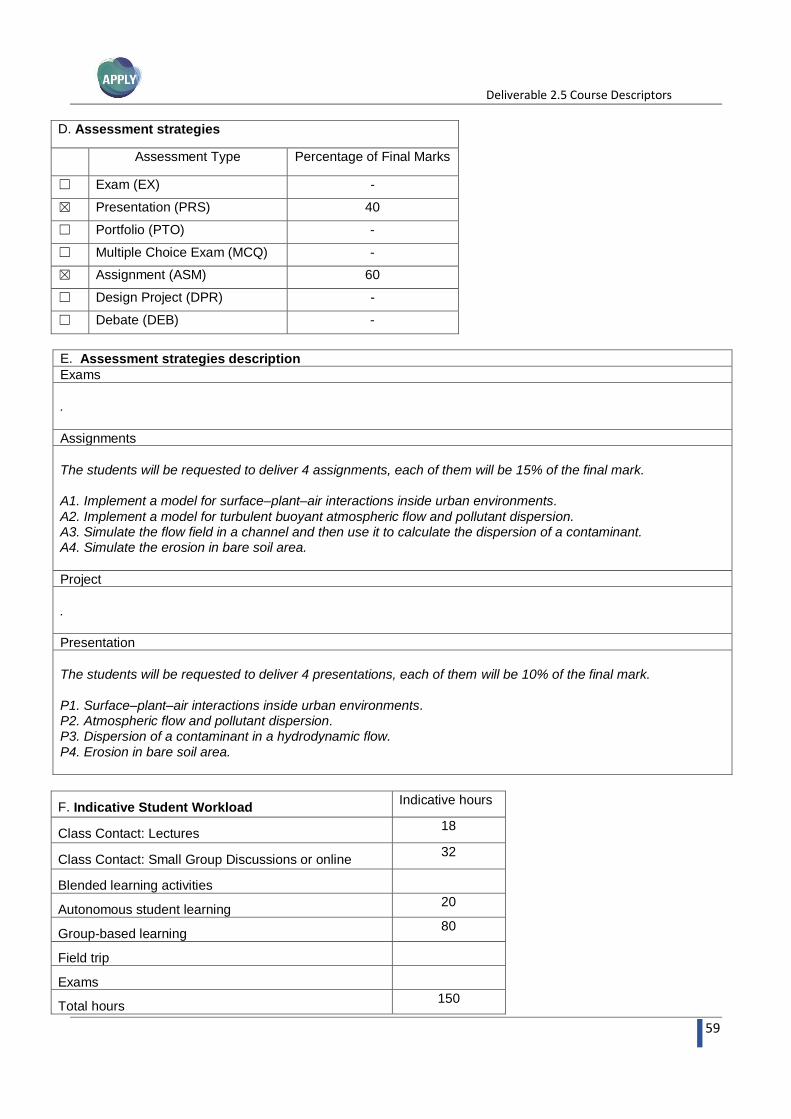
Deliverable 2.5 Course Descriptors
59
D. Assessment strategies
Assessment Type Percentage of Final Marks
☐ Exam (EX) -
☒ Presentation (PRS) 40
☐ Portfolio (PTO) -
☐ Multiple Choice Exam (MCQ) -
☒ Assignment (ASM) 60
☐ Design Project (DPR) -
☐ Debate (DEB) -
E. Assessment strategies description
Exams
.
Assignments
The students will be requested to deliver 4 assignments, each of them will be 15% of the final mark. A1. Implement a model for surface–plant–air interactions inside urban environments.
A2. Implement a model for turbulent buoyant atmospheric flow and pollutant dispersion. A3. Simulate the flow field in a channel and then use it to calculate the dispersion of a contaminant. A4. Simulate the erosion in bare soil area.
Project
.
Presentation
The students will be requested to deliver 4 presentations, each of them will be 10% of the final mark.
P1. Surface–plant–air interactions inside urban environments. P2. Atmospheric flow and pollutant dispersion. P3. Dispersion of a contaminant in a hydrodynamic flow.
P4. Erosion in bare soil area.
F. Indicative Student Workload Indicative hours
Class Contact: Lectures 18
Class Contact: Small Group Discussions or online 32
Blended learning activities
Autonomous student learning 20
Group-based learning 80
Field trip
Exams
Total hours 150

Deliverable 2.5 Course Descriptors
60
G. Indicative Content
Module
Content Content Sources/Resources (e.g. texts, web resources, journal articles, equipment resources)
1 Introduction PowerPoints / PDFs ,
Lecture notes, A personal computer with a programing environment Books:
Environmental modelling : finding simplicity in complexity / [edited by] John Wainwright and Mark Mulligan. – 2nd ed., 2013 by John Wiley &
Sons, Handbook of Environmental Fluid Dynamics, / [edited by] H. J. S. Fernando, 2013 CRC Press by Taylor &
Francis Group Computational fluid dynamics: applications in environmental hydraulics/ editors,
Paul D. Bates, Stuart N. Lane, Robert I. Ferguson, 2005 John Wiley & Son.
2 Modelling techniques
3 Buildings and urban environment
4 Simulation of air flow in urban environment
5 Atmospheric dispersion modelling
6 Simulation of pollutant dispersion
7 Environmental hydraulics and transport processes
8 Pollutant transport in a channel flow
9 Soil erosion
10 Erosion in bare soil area

Deliverable 2.5 Course Descriptors
61
13. Multiphase Flows
Course Title: Multiphase Flows
Course Code: APPLY E6
Course Type: Core ☐ Elective ☒
Credits: 6 ECTS Semester: 2
Course Coordinators: UP (George Vafakos – Polycarpos Papadopoulos)
Course Review: UM (Ramesh T Subramaniam, Ramesh Kasi)
A. Course Description
This course is designed to provide students with a strong background on fundamental fluid mechanics, the
necessary understanding of the dynamics of multiphase flow and the essential CFD tools for such kind of flows.
In this course, after a description of the mathematical and physical aspects of multiphase flows, a detailed overview of the most important computational models will be given. The primary computational models that will be discussed are targeted in the continuous phase (two liquid mixing, liquid-gas flow, etc.), such as the Euler-
Euler and the volume-of-fluids model, and in the discrete phase (particles, droplets or bubbles), such as the Euler-Lagrangian models. The students will be called upon to create computer scripts, either in a programming language of their choosing or using the open-source OpenFOAM library, in order to gain hands-on experience in
successfully solving an applied multiphase problem.
B. Modules
Module name Introduction Number 1
Total hours 13 Class hours 8 Autonomous study hours 5
Module description
Basic definitions. Importance of dimensionless numbers. Notation of important fluid variables. Classification of
multiphase flows. Flow patterns and regimes. Horizontal and vertical two-phase flows. Instabilities. Eulerian and
Lagrangian description of fluid motion. Mass, momentum and energy conservation equations for single and multi-phase flows. Mixture model equations. Two-fluid model equations. Boundary conditions in two-phase flow. Interaction with turbulence.
Module assessment methodology
Assignment 1
Assignment Topic: Exercises on the understanding of multi-phase flows. Type of Assignment: Personal assignment. Estimated study hours: 5
Module name Liquid-Gas Two-Phase Flows (Theory) Number 2
Total hours 8 Class hours 8 Autonomous study hours
Module description
Flow pattern classification. Flow regime maps for vertical and horizontal flow. Bubble flow. Slug flow. Churn flow.
Annular flow. Dispersed flow. Flow regimes limits. Separated flow instabilities. Frictional pressure drop in disperse, homogenous and separated flows. Darcy–Weisbach equation. Pressure drop models by Lockhart-Martinelli, Baroczy-Chisholm, Beggs-Brill, Friedel, etc. Homogenous flows. Gas/bubble dynamics flows.

Deliverable 2.5 Course Descriptors
62
Module assessment methodology This module will be assessed in the assignment A2.
Module name Liquid-Gas Two-Phase Flows (Project) Number 3
Total hours 12 Class hours 2 Autonomous study hours 10
Module description
Explanation and presentation of the project by the teacher. The students will perform an algebraic computation of pressure drop behaviour in two-phase liquid-gas pipe flow, using realistic conditions (surface roughness, friction factor, geometry bends, etc.) and compare results using various multiphase models. There will be multiple projects to choose from.
Module assessment methodology
Assignment 2 Assignment Topic: Students shall create a dynamic executable computer program that calculates and
presents the requested results. A report deliverable is required. Type of Assignment: Personal assignment. Estimated study hours: 10
Module name Particle Motion, Bubble/Droplets Formation and Cavitation Number 4
Total hours 13 Class hours 8 Autonomous study hours 5
Module description
Single particle motion. Flow around a sphere. Free flow velocity. Grain’s size and concentration effect on free
flow drag. Schiller-Naumann drag model. Hydraulic transport of solids. Particle’s flow motion. Bubble shape. Marangoni effects and Bjerkes forces. Rayleigh-Plesset equation. Thermal and non-thermal bubble growth and collapse. Cavitation bubbles: shape distortion and noise.
Module assessment methodology
Assignment 3
Assignment Topic: Mathematical exercises on particle motion, bubble/droplets formation and cavitation. Type of Assignment: Personal assignment. Estimated study hours: 5
Module name Numerical Modelling I: Euler-Lagrangian Model (Theory) Number 5
Total hours 3 Class hours 3 Autonomous study hours
Module description
Newton’s second law for single particle’s motion. Lagrangian particle tracking. Force balance. Drag, lift, buoyancy, gravitational and Brownian forces. Particle’s relaxation time. Visualization of particle’s trajectory.
Module assessment methodology

Deliverable 2.5 Course Descriptors
63
This module will be assessed in the assignment A4.
Module name Numerical Modelling I: Euler-Lagrangian Model (Project) Number 6
Total hours 32 Class hours 2 Autonomous study hours 30
Module description
Explanation and presentation of the group project by the teacher. The students shall create a CFD numerical
code in a programming language of their choosing, using the Euler-Lagrangian model, in order to model the motion of solid particles in fully developed or developing 2D incompressible laminar flow.
Module assessment methodology
Assignment 4
Assignment Topic: Students shall create a CFD numerical code in a programming language of their choosing, in order to solve the equations and visualize the flow.
Type of Assignment: Team project. A report deliverable is required. Estimated study hours: 30
Module name Numerical Modelling I: Euler-Lagrangian Model (Results & Discussion)
Number 7
Total hours 3 Class hours 3 Autonomous study hours
Module description
The students will present their results in the classroom, along with a brief explanation of their code and techniques.
Module assessment methodology
This module will be assessed in the assignment A4.
Module name Numerical Modelling II: Volume-of-Fluids Model (Theory) Number 8
Total hours 3 Class hours 3 Autonomous study hours
Module description
Newton’s second law for single particle’s motion. Lagrangian particle tracking. Force balance. Drag, lift, buoyancy, gravitational and Brownian forces. Particle’s relaxation time. Visualization of particle’s trajectory.
Module assessment methodology
This module will be assessed in the assignment A5.
Module name Numerical Modelling II: Volume-of-Fluids Model (Project) Number 9
Total hours 32 Class hours 2 Autonomous study hours 30

Deliverable 2.5 Course Descriptors
64
Module description
Explanation and presentation of the group project by the teacher. The students will create a computational code based in OpenFOAM, starting from a simplistic incompressible solver, and building up to a VOF multiphase
solver.
Module assessment methodology
Assignment 5
Assignment Topic: The solution of a benchmark simple fluid dynamic multiphase case study, using a VOF solver, constructed with the OpenFOAM software tool.
Type of Assignment: Personal project. A report deliverable is required. Estimated study hours: 30
Module name Numerical Modelling II: Volume-of-Fluids Model (Results & Discussion)
Number 10
Total hours 3 Class hours 3 Autonomous study hours
Module description
The students will present their results in the classroom, along with a brief explanation of their solver and input parameters.
Module assessment methodology
This module will be assessed in the assignment A5.
Module name Numerical Modelling III: Euler-Euler Model (Theory) Number 11
Total hours 3 Class hours 3 Autonomous study hours
Module description
Full Euler-Euler model for multiphase flows. Link momentum equation for each phase. Liquid-liquid / liquid-solid mixing. Introduction to OpenFOAM multiphase solvers. Complex multiphase flows with turbulence, compressibility and heat transfer effects
Module assessment methodology
This module will be assessed in the assignment A6.
Module name Numerical Modelling III: Euler-Euler Model (Project) Number 12
Total hours 22 Class hours 2 Autonomous study hours 20
Module description
Explanation and presentation of the group project by the teacher. The students shall simulate a complex flow using the OpenFOAM platform, using the multiphase tools that are provided. The case could contain one or

Deliverable 2.5 Course Descriptors
65
more of the following phenomena: heat transfer, turbulence, non-Newtonian fluids, flow through porous media, etc.
Module assessment methodology
Assignment 6
Assignment Topic: Computationally model a complex multiphase flow for various parameters, fluids and working conditions using the software tool OpenFOAM.
Type of Assignment: Personal project. A report deliverable is required. Estimated study hours: 20
Module name Numerical Modelling III: Euler-Euler Model (Results & Discussion) Number 13
Total hours 3 Class hours 3 Autonomous study hours
Module description
The students will present their results in the classroom, along with the post-process visualization techniques and
a brief explanation of the physical phenomena that observed in the flow.
Module assessment methodology
This module will be assessed in the assignment A6.
C. Course Learning Outcomes. Upon completion of the course, students will be able to
1. Gain a valuable theoretical background in multiphase flows.
2. Understand the applications of multiphase flows in the industry.
3. Understand the necessity of numerical modelling in such complex flows.
4. Apply various models for multiphase flows.
5. Have a deep understanding of the available multiphase solvers provided by the OpenFOAM software.
6. Predict the behaviour of multiphase flows in internal pipe flows, in realistic industrial conditions.
Transferable Skills: - Code development and verification.
- Knowledge of OpenFOAM multiphase solvers. - Knowledge of manipulating OpenFOAM available solvers and cases towards one’s needs. - Understanding the Navier-Stokes equations, and their association with multiphase flows.
D. Assessment strategies
Assessment Type Percentage of Final Marks
☐ Exam (EX) -
☒ Presentation (PRS) 40

Deliverable 2.5 Course Descriptors
66
☐ Portfolio (PTO) -
☐ Multiple Choice Exam (MCQ) -
☒ Assignment (ASM) 60
☐ Design Project (DPR) -
☐ Debate (DEB) -
E. Assessment strategies description
Assignments
The students will be requested to deliver 6 assignments, two of which are theoretical exercises, and the other 4
are computational projects. The successful project completion will result in the 60% of their final mark. - Assignment 1: Solve simple mathematical exercises on understanding of multiphase flows. (Module 1) - Assignment 2: Create a computational code that computes the pressure drop and other important
parameters for liquid-gas two-phase internal incompressible flows. (Module 3) - Assignment 3: Solve simple mathematical exercises on particle motion, bubble/droplets formation and
cavitation. (Module 4)
- Assignment 4: Create a computational code that solves the multiphase flow equations using the Euler/Lagrange model. (Module 6)
- Assignment 5: Create a solver using the open-source library OpenFOAM, which will use the volume-of-
fluids model to describe a multiphase flow. (Module 9) - Assignment 6: Use the incorporated OpenFOAM tools to describe a complex multiphase flow that
includes various physical phenomena, such as turbulence, heat/mass transfer, etc. (Module 12)
-
Presentation
There will be three classroom presentations of the three last projects, where the teachers will assess the student’s work, discuss their results, and evaluate their effort. The presentation will be conducted in Modules 7, 10 and 13. It will represent the 40% of their final mark.
F. Indicative Student Workload Indicative hours
Class Contact: Lectures 41
Class Contact: Small Group Discussions or online -
Blended learning activities -
Autonomous student learning 70
Group-based learning 30
Field trip -
Exams (presentations) 9
Total hours 150
G. Indicative Content
Module
Content Content Sources/Resources (e.g.
texts, web resources, journal
articles, equipment resources)
1 Introduction

Deliverable 2.5 Course Descriptors
67
2 Liquid-Gas Two-Phase Flows (Theory)
PowerPoints / PDFs, Lecture notes, Scientific books.
3 Liquid-Gas Two-Phase Flows (Project)
4 Particle Motion, Bubble/Droplets Formation and Cavitation
5 Numerical Modelling I: Euler-Lagrangian Model (Theory)
6 Numerical Modelling I: Euler-Lagrangian Model (Project)
7 Numerical Modelling I: Euler-Lagrangian Model (Results & Discussion)
8 Numerical Modelling II: Volume-of-Fluids Model (Theory)
9 Numerical Modelling II: Volume-of-Fluids Model (Project)
10 Numerical Modelling II: Volume-of-Fluids Model (Results & Discussion)
11 Numerical Modelling I: Euler- Euler Model (Theory)
12 Numerical Modelling I: Euler- Euler Model (Project)
13 Numerical Modelling I: Euler- Euler Model (Results & Discussion)
Additional information
The students of this course are required to have basic background in programming, general fluid dynamics and calculus, either by their undergraduate education, or from previous courses of the present master program. The preferred programming languages are Matlab or python.
Additional information about multiphase flows can be found in the following books:
Brennen, C. (2005). Fundamentals of Multiphase Flow. Cambridge: Cambridge University Press. doi:10.1017/CBO9780511807169
Guan Heng Yeoh, Jiyuan Tu. (2019). Computational Techniques for Multiphase Flows (Second Edition). Butterworth-Heinemann. ISBN 9780081024539. https://doi.org/10.1016/B978-0-08-102453-9.12001-X.

Deliverable 2.5 Course Descriptors
68
14. Modelling and Simulation of Energy Systems
Course Title: Modeling and Simulation of Energy Systems (Energy)
Course Code: APPLY E7
Course Type: Core ☐ Elective ☒
Credits: 6 ECTS ☒
Semester:
Course Coordinator: Naresuan University (NU)
Course Review: Chiang Mai University (CMU)
A. Course Description
Will examine specific flows that occur in power plants, cogeneration systems, propulsion plants, heating and cooling applications etc. It will involve an introduction to the main flows that are encountered in such systems and a presentation of the numerical tools that are available for their simulation. The focus of the course will be in
the utilization of CFD as a means of optimizing the energy systems and determining the limiting values of critical operational parameters.
B. Modules
Module name Introduction Number 1
Total hours 9 Class hours 2 (Lec) 2 (Lab)
Autonomous study hours 5
Module description
Overview of utilising CFD technique for flow study and design optimization of components in energy systems.
Practice in flow simulation of a simple heat exchanger using CFD software.
Module assessment methodology
Practice: a simple heat exchanger: Simulation and design optimization
Module name Thermal power plant Number 2
Total hours 36 Class hours 8 (Lec)
8 (Lab) Autonomous study hours 20
Module description
Using CFD software for the simulation of main components in a thermal power plant as follows: Steam boiler, Steam turbine and Furnace. Explanation of the theories related in flow phenomena each component. Design optimization of operational parameters.
Module assessment methodology
Assignment 1 : Steam boiler : Simulation and design optimization Assignment 2 : Steam turbine: Simulation and design optimization Assignment 3 : Furnace: Simulation and design optimization

Deliverable 2.5 Course Descriptors
69
Module name Hydro power plant Number 3
Total hours 18 Class hours 4 (Lec) 4 (Lab)
Autonomous study hours 5
Module description
Using CFD software for the flow simulation of main components in a hydro power plant. The theories and equations related in flow simulation of water turbine. Design optimization of operational parameters.
Module assessment methodology
Assignment 4 : Hydro turbine : Simulation and design optimization
Module name Wind power plant Number 4
Total hours 18 Class hours 4 (Lec)
4 (Lab) Autonomous study hours 10
Module description
Using CFD software for the flow simulation of main components in wind power plant. The theories and equations related in flow simulation of wind turbine. Design optimization of operational parameters.
Module assessment methodology
Assignment 5: Wind turbine : Simulation and design optimization
Module name Propulsion plant Number 5
Total hours 18 Class hours 4 (Lec) 4 (Lab)
Autonomous study hours 10
Module description
Using CFD software for the flow simulation of main components in a propulsion plant. The theories and
equations related in flow simulation of gas turbine. Design optimization of operational parameters.
Module assessment methodology
Assignment 6: Gas turbine : Simulation and design optimization
Module name Heating: Solar collector Number 6
Total hours 18 Class hours 4 (Lec)
4 (Lab) Autonomous study hours 10
Module description
Using CFD software for the flow simulation of a solar collector. The theories and equations related in flow simulation of the solar collector. Design optimization of operational parameters.
Module assessment methodology
Assignment 7: Heating: Solar collector : Simulation and design optimization
Module name Cooling: Condenser Number 7
Total hours 18 Class hours 4 (Lec) Autonomous study hours 10

Deliverable 2.5 Course Descriptors
70
4 (Lab) Module description
Using CFD software for the flow simulation of a condenser. The theories and equations related in flow simulation of the condenser. Design optimization of operational parameters.
Module assessment methodology
Assignment 8 : Cooling : Condenser : Simulation and design optimization
C. Course Learning Outcomes. Upon completion of the course, students will be able to
1. The student will be able to work on the flow simulation including design optimization of main components in
the thermal power plant.
2. The student will be able to work on the flow simulation including design optimization of a main component in the hydro power plant.
3. The student will be able to work on the flow simulation including design optimization of a main component in the wind power plant.
4. The student will be able to work on the flow simulation including design optimization of main components in the propulsion plant.
5. The student will be able to work on the flow simulation including design optimization of a solar collector.
6. The student will be able to work on the flow simulation including design optimization of a condenser.
Transferable Skills: - Knowledge of using a commercial CFD software as tool for the flow simulation in energy systems
D. Assessment strategies
Assessment Type Percentage of Final Marks
☒ Exams (EX) 40
☐ Presentation (PRS) -
☐ Portfolio (PTO) -
☐ Multiple Choice Exam (MCQ) -
☒ Assignment (ASM) 60
☐ Design Project (DPR) -
☐ Debate (DEB) -
E. Assessment strategies description
Exams
Two exams of 40 % will be found in the mid-term period and the end of course. Each assessment carries 20 % of the final marks. The numerical simulation using CFD of case studies will be assigned in each exam.
Assignments
Eight assignments of the simulation and optimization in each module will be requested for practice.

Deliverable 2.5 Course Descriptors
71
Assignment 1: Steam boiler
Assignment 2: Steam turbine Assignment 3: Furnace Assignment 4: Hydro turbine
Assignment 5: Wind turbine Assignment 6: Gas turbine Assignment 7: Solar collector
Assignment 8: Condenser
F. Indicative Student Workload Indicative hours
Class Contact: Lectures 30
Class Contact: Computer Laboratory 30
Blended learning activities
Autonomous student learning 75
Group-based learning
Field trip
Exams 15
Total hours 150
G. Indicative Content
Module
Content Content Sources/Resources (e.g. texts, web
resources, journal articles, equipment resources)
1 Week 1 : Introduction PowerPoint, Textbook, Computer laboratory, CFD
Commercial software 2 Week 2-5 :Thermal power plant
3 Week 6-7 :Hydro power plant
4 Week 8-9 :Wind power plant
5 Week 10-11 :Propulsion plant
6 Week 12-13 :Heating application : Solar collector
7 Week 14-15 :Cooling Application: Condenser
Text book:
1. ANSYS FLUENT User's Guide 2. ANSYS FLUENT Theory Guide
Deliverable 2.5 Course Descriptors
72
15. Int. to the Numerical Simulation of Environmental and Atmospheric Flows
Course Title: Introduction to the Numerical Simulation of Environmental and Atmospheric Flows
Course Code: APPLY E8
Course Type: Core ☒ Elective
Credits: 6 ECTS
Semester: 1
Course Coordinator: UPC (Enrique García-Melendo)
Course Review: VIT
A. Course Description
In this course the student is introduced to the application of the Navier-Stokes (N-S) equations and several aspects of thermodynamical applications to understand the fundamentals of atmospheric /environmental fluid flows. The Navier-Stokes equations are then simplified to a Shallow Water (SW) model applied to a planetary
spherical or ellipsoidal surface. The course is based on theory and numerical exercises and projects where the students will have to apply the learned theory and ultimately build their own model. This course will be based on an open source language, like Python (preferably), or, Fortran, or a commercial one, such as Matlab.
B. Modules
Module name Fundamentals of Atmospheric Processes Number 1
Total hours 37 Class hours 12 Autonomous study hours 25
Module description
N-S equations. Coriolis force. Rossby number. Equations of motion in spherical coordinates. The f-plane, the 𝛽-
plane. Geostrophic flows. Vorticity and potential vorticity. Hydrostatic balance. Derivation of the Potential Temperature. States of stability. Stratification and diffusion problems. Parcel Concepts. Thermal wind equation. General Circulation. Simulation techniques in Large scale flows.
Module assessment methodology
Open Book examination to test familiarity with (i) theoretical Concepts (ii) applied concepts Assignment : Resolving computer exercises. Using a GCM model following a WRF (Weather Research and
Forecasting) Tutorial. Students will learn the fundamentals by experimenting with either their own codes or by using already existing models such as the WRF. Simple code development to ascertain stability states of the atmosphere (stable, unstable, neutral), Coding simple diffusion problems under various states of stability
Module name Thermodynamics and Boundary Layer Processes Number 2
Total hours 38 Class hours 13 Autonomous study hours 25
Module description
Principles of Energy, Entropy and Enthalpy. The First and Second law of Thermodynamics. Thermodynamic Energy Equations. Vertical structure and change of state due to vertical motions. Moist and Pseudo-adiabatic processes. Expanded continuity equations. Cloud-fog physics. Boundary layer physics. Applications of the momentum equation in urban boundary layer.
Module assessment methodology
Open Book Examination to test knowledge of (i) Thermodynamical extensions over large scale flows (ii) Boundary layer/Urban Meteorology
Deliverable 2.5 Course Descriptors
73
Assignment : (i) Solving chosen case studies sourced locally to simulate dispersion of gases and particles from point (industrial stacks), line (traffic laden highway) and area sources (crop residue burning over farmlands)
(ii) Simulating a cloud/fog event in an urban boundary layer using a thermodynamic parcel model
Module name The SW model theory and numerical methods Number 3
Total hours 24 Class hours 12 Autonomous study hours 12
Module description
Approximations to N-S equations: Shallow Water (SW) equations, Boussinesq and Anelastic approximations. Model for large scale oceanic or atmospheric simulations. Approximations on free surface SW equations. Potential vorticity and conservation properties. Finite differences. Numerical schemes for the advection term. Basic and energy conserving schemes. Flux limiters. The Courant number. The Rossby radius of deformation.
Module assessment methodology
Modules 3 and 4 are assessed during the implementation of a fully functional SW model in an open source language such as in Python, Fortran or in commercial software such as Matlab.
Module name SW model implementation Number 4
Total hours 51 Class hours 12 Autonomous study hours 39
Module description
SW model implementation. Staggered grids. MMS validation, advection implementation, dynamic pressure, time integration and Coriolis acceleration. Mass conservation equation implementation. Boundary conditions. Cartesian and ellipsoidal coordinates. Introduction of zonal jets, currents. Large scale perturbations and geostrophic equilibrium.
Module assessment methodology
Modules 3 and 4 are assessed during the implementation of a fully functional SW model in an open source
language such as in Python or Fortran or in commercial software such as Matlab .
C. Course Learning Outcomes. Upon completion of the course, students will be able to
1. Understand the basic principles of atmospheric physics.
2. Understand the basic particularities of the atmpshere/ocean dynamics.
3. Understand some de thermodynamic aspects of the atmosphere and its interaction with the earth surface.
4. Elaborate/use code to simulate the behavior of different aspects of the atmosphere/oceans.
5. Code a fully functional SW model for atmospheric/oceanic applications on Earth or other planets.
Transferable Skills: - Understand the nature of SW equations.
- Code development and verification. - Complete model implementation

Deliverable 2.5 Course Descriptors
74
D. Assessment strategies
Assessment Type Percentage of Final Marks
☒ Exam (EX) 15
☒ Presentation (PRS) 15
☐ Portfolio (PTO) -
☐ Multiple Choice Exam (MCQ) -
☒ Assignment (ASM) 20
☒ Design Project (DPR) 50
☐ Debate (DEB) -
E. Assessment strategies description
Exams
In modules 1 and 2 students will have to demonstrate not only a working familiarity, but also an in depth understanding of the applications of the Navier Stokes Equation to distinguish between the relative importance
of the Pressure Gradient, Coriolis Force and Viscous Force in atmospheric processes. Additionally, they must demonstrate an understanding of diffusion, stratification and processes of turbulent transport of tracers in the form of gases and particles from real world examples sourced from urban and industrial processes.
Assignments
In modules 1 and 2 assignments will focus on (i) Simple code development to ascertain stability states of the atmosphere (stable, unstable, neutral), Coding simple diffusion problems under various states of stability (ii) Solving chosen case studies sourced locally to simulate dispersion of gases and particles from point (industrial
stacks), line (traffic laded highway) and area sources (crop residue burning over farmlands) In modules 3 and 4 students will have to implement different modules of the SW model with its corresponding
MMS validation, (i) boundary conditions, (ii) advection, (iii) dynamical pressure forcing, (iv) time integration, (v) Coriolis term, (vi) potential vorticity, (vii) perturbation injection, (viii) zonal winds/current introduction, (forced versus geostrophic equilibrium) , (xix) vortex/pertubation introduction.
Project
In modules 1 and 2 the following projects will be undertaken (i) Using established codes such as simple test cases of the most basic version of the WRF model to generate forecasts of cyclonic activity / precipitation events (ii) Develop a simple Gaussian Plume diffusion code in Python with its own graphical interface to
demonstrate diffusion of pollutants from point, line and area sources (iii) Use of a simple cloud parcel model to simulate fog/cloud events
Building a fully functional SW model. In two steps. Step 1: Building the initial core of the model by simulating in a fully periodic domain in Cartesian coordinates gravity waves. Step 2: Introducing the Coriolis force and spherical and/or ellipsoidal coordinates, channel boundary conditions, zonal winds, and a perturbation to build a moldel to
simulate de Great Red Spot of Jupiter or Saturn’s 2010 Great Storm.
Presentation
For Modules 1 and 2, the students will have to give one class presentation (40 minutes) and additionally will submit abstracts for VIT’s annual SET (Science Engineering and Technology Conference) and prepare a conference Presentation (15 minutes).
For Modules 3 and 4, the students will have to give one class presentation of his SW project showing their results on the Great Spot of Jupiter or Saturn’s 2010 Great Storm.

Deliverable 2.5 Course Descriptors
75
F. Indicative Student Workload Indicative hours
Class Contact: Lectures 50
Class Contact: Small Group Discussions or online
Blended learning activities
Autonomous student learning 100
Group-based learning
Field trip
Exams
Total hours 150
G. Indicative Content
Module
Content
1 Fundamentals of Atmospheric Processes:
1. Fundamentals of Atmospheric Modelling. Mark
Jacobson. 2nd Edition (2005). Publisher: ISBN-10: 0521548659 ISBN-13: 978-0521548656. Cambridge University Press. U.K.
2. Computational Methods in Environmental Fluid
Mechanics. Kolditz Olaf. 1st Edition (2002). ISBN 978-3-540-42895-4. Springer.
3. Atmosphere, Ocean and Climate Dynamics. John
Marshall and Alan Plumb. 1st Edition (2007). ISBN-10: 0125586914 | ISBN-13: 978-0125586917 | Elsevier Academic Press. USA.
2 Thermodynamics and Boundary Layer Processes
3 The SW model theory and numerical
methods
4. Pedlosky, “Geophysical Fluid Dynamics”, Springer.
5. Benoit Cushman-Roisin & Jean-Marie Beckers, “Introduction to Geophysical Fluid Dynamics, Physical and Numerical Aspects”, Academic Press.
6. 3.Jochen Kämpf, “Ocean Modelling for Beginners”. Springer.
7. 4.Versteeg, H. “An Introduction to Computational Fluid Dynamics: The Finite Volume Method”, Pearson

Deliverable 2.5 Course Descriptors
76
16. Introduction to Finite Element Analysis of Solids and Fluids
Course Title: Introduction to Finite Element Analysis of Solids and Fluids
Course Code: APPLY E9
Course Type: Core ☐ Elective ☒
Credits: 6 ECTS
Semester: 1
Course Coordinator: CMU (Arpiruk Hokpunna)
Course Review: NU ()
A. Course Description
Covers theory and method of linear and non-linear finite element procedures solving solid and fluid mechanics, heat and mass transfer problems. Theoretical and fundamental procedure in one dimension will be covered in detail. Hands-on experiment with 1D and 2D codes will be given and followed by 2D and 3D experiment with
opensource and commercial-software.
B. Modules
Module name Introduction to Finite Element Method Number 1
Total hours 21 Class hours 9 Autonomous study hours 12
Module description
- Introduction to interlink between spatial discretization, equation discretization and numerical
approximation. - Basic concept of node and element - Introduction to method of weighted residual and the finite element approximation
- Element and shape function. - Nodal vs. Modal FEM. - Hands on practice on the application of FEM/FVM on 1D heat conduction-convection equation (CDE).
Module assessment methodology
Assignment 1 : Derivation of 1D FEM for convection-diffusion equation Assignment 2 : Python or Octave programing of FEM solving 1D convection-diffusion equation
Module name Two dimensional FEM and higher order element Number 2
Total hours 21 Class hours 9 Autonomous study hours 12
Module description
- Introduction to 1D higher-order element - Two-dimensional triangular linear element and quadratic element
- Two-dimensional quadrilateral elements - Introduction to standard FEM (Galerkin, Rtiz) - Numerical Integration
Module assessment methodology

Deliverable 2.5 Course Descriptors
77
Assignment 1 : Solve 1D CDE using higher-order element and compare convergence rate and solution time with result form the last module.
Assignment 2 : Use symbolic software to solve 2D CDE using 1,4 and 16 linear elements and compare the accuracy with quadratic element on 1 and 4 elements. Assignment 3: 1D and 2D numerical integration
Module name Application to Solid Mechanics: one-dimensional Beam Number 3
Total hours 15 Class hours 6 Autonomous study hours 9
Module description
- Kinematics, equilibrium and material laws - Beam element, stiffness matrix and the variational approach - Transverse beam load (concentrated and distributed forces)
- Planar frame structure
Module assessment methodology
Assignment 1 : Solve two problems of 1D axial load problem Assignment 2 : Solve two problems of 1D transverse load problem
Assignment 3: Solve one problem of Planar frame structure
Module name Application to Solid Mechanics: Multi-dimensional problems Number 4
Total hours 12 Class hours 6 Autonomous study hours 6
Module description
- Beam element stiffness matrix of triangular element in 2D - Forming two-dimensional discrete system of FEM
Module assessment methodology
Assignment 1 : Solve two problems of 2D beam bending
Module name Application to Fluid Mechanics Number 5
Total hours 21 Class hours 9 Autonomous study hours 12
Module description
- Discrete and semi-discrete FEM for fluid flow - Split method and penalty method
- Discrete mass conservation and energy conservation
Module assessment methodology
Assignment 1 : Use opensource software to solve a two-dimensional flow problems
Module name Analysis of Finite element method and parallel solution procedure Number 6

Deliverable 2.5 Course Descriptors
78
Total hours 21 Class hours 9 Autonomous study hours 12
Module description
- Review of Linear algebra and introduction to Functional Analysis - Errors, consistency, stability, and convergence of FEM
- Iterative and parallel solver for large matrices
Module assessment methodology
Assignment 1 : Perform error analysis on convection and diffusion equation Assignment 2 : Conduct speedup study on parallel iterative solver applied to FEM linear system
C. Course Learning Outcomes. Upon completion of the course, students will be able to
1. Demonstrate understanding of fundamental concept of Finite Element Method
2. Apply Finite Element Method to solve problems related to Fluid Mechanics and Solid Mechanics
3. Able to utilize opensource FEM software to solve, interpret analyze engineering problems.
Transferable Skills: - Code development and verification.
- Ability to use opensource software to visualize and analyze data. For example, gnuplot, TikZ, paraview.
D. Assessment strategies
Assessment Type Percentage of Final Marks
Exam (EX) 40
Presentation (PRS) 10
☐ Portfolio (PTO) -
☐ Multiple Choice Exam (MCQ) -
Assignment (ASM) 30
Design Project (DPR) 20
☐ Debate (DEB) -
E. Assessment strategies description
Exams
This course will have 2 exams. The first one, 2 months after the beginning of the course, with a 15% of the final
mark weight and a second one, at the end of the course, with a 25% of the final mark weight.
Assignments
The students will be requested to deliver 12 assignments. Assignment 1 to 10 weight are 20% of the final mark and the last two are 10%.
Project

Deliverable 2.5 Course Descriptors
79
A term project is assigned to the students after the comlpletion of the 4th module. Each goup will consist of 2 – 3 students. A set of scenarios will be given for choosing. The students must clarify their responsibility in the
project and present their parts during the project presentation.
Presentation
Each student shall select an academic paper related to Finite Element and present the paper to the class within 45 minute. The class shall have 15 minutes to ask the questions. Samples paper will be given to the student
such that they can choose a similar paper.
F. Indicative Student Workload Indicative hours
Class Contact: Lectures 30
Class Contact: Small Group Discussions or online 15
Blended learning activities ---
Autonomous student learning 63
Group-based learning 36
Field trip ---
Exams 6
Total hours 150
G. Indicative Content
Module
Content Content Sources/Resources (e.g. texts, web
resources, journal articles, equipment resources)
1 Introduction to Finite Element Method PowerPoint, video lecture, PDF lecture notes,journal
article, Text books:
- Fundamentals of the Finite Element Method
for Heat and Fluid Flow , Roland W. Lewis Perumal Nithiarasu Kankanhalli N. Seetharamu ,2004 by John Wiley & Sons,
- The Finite Element Method for Fluid Dynamics , Zienkiewicz, Taylor, Nithiarasu, 7th ed., 2013, by Butterworth-Heinemann
- MATLAB Codes for Finite Element Analysis, A. J. M. Ferreira and N. Fantuzzi, 2nd ed., 2009 by Springer
2 Two dimensional FEM and higher order element
3 Application to Solid Mechanics: one-dimensional Beam
4 Application to Solid Mechanics: Multi-dimensional problems
5 Application to Fluid Mechanics
6 Analysis of Finite element method and parallel solution procedure
Additional information
Symbolic programming, usage of opensource are given exclusively as online primer and video lectures. Students are expected to study them during the autonomous study time.

Deliverable 2.5 Course Descriptors
80
17. Transport Phenomena
Course Title: Transport Phenomena
Course Code: APPLY Elective course
Course Type: Core ☐ Elective ☒
Credits: 6 ECTS ☒
Semester:
Course Coordinator: Naresuan University (NU)
Course Review: Chiang Mai University (CMU)
A. Course Description
Analytic method of solving transport problems: momentum, energy and species. Transport by molecular motion; one-dimensional transport in laminar flow and in solids. Transport in continuum: isothermal, non-isothermal and multi-component systems. Transport in laminar flow for both Newtonian and non-Newtonian fluids and in solids with two independent variables. Numerical solution for transport phenomena problems. Case studies.
B. Modules
Module name Momentum Transport Number 1
Total hours 47 Class hours 15 (Lec) 7 (Lab)
Autonomous study hours 25
Module description
Introduction to molecular momentum transport; Newtonian vs non-Newtonian fluid viscosity models; Shell balances; Equation of change for isothermal systems; Momentum transport problem with 2 independent
variables
Module assessment methodology
Practice: Analytical solutions for Newtonian fluid flow through different coordinate systems such as the
Cartesian, the cylindrical, and the spherical coordinates. Assignment : 2D and 3D simulation of non-Newtonian fluid flow
Module name Energy Transport Number 2
Total hours 41 Class hours 10 (Lec)
6 (Lab) Autonomous study hours 25
Module description
Introduction of mechanism of energy transport; Shell balances on energy transport for 1D problem; Equation of
change for nonisothermal system; Energy transport problem with 2 independent variables
Module assessment methodology
Practice: Analytical solutions for energy transport in different coordinate systems Assignment : 2D and 3D simulation of energy transport
Module name Species (Mass) Transport Number 3

Deliverable 2.5 Course Descriptors
81
Total hours 47 Class hours 15 (Lec) 7 (Lab)
Autonomous study hours 25
Module description
Diffusivity and mechanism of mass transport; Shell balances on mass transport for 1D problem; Equation of
change for multicomponent systems; Mass transport problem with 2 independent variables
Module assessment methodology
Practice : Analytical solutions for mass transport in different coordinate systems
Assignment : 2D and 3D simulation of mass transport
C. Course Learning Outcomes. Upon completion of the course, students will be able to
1. Students will be able to develop analytical solutions for momentum, energy and mass transport phenomena.
2. Students will be able to use computational software to solve transport phenomena problems and present
their results in the appropriate ways.
3. Students will be able to discuss the solved results by using their knowledge in transport phenomena.
Transferable Skills: - Setting up correct differential equations for each or multiple phenomena.
- Using a commercial CFD software as tool for simulation of each or multiple phenomena. - Discussion skill on obtaining both analytical and numerical solutions.
D. Assessment strategies
Assessment Type Percentage of Final Marks
☒ Exams (EX) 20
☒ Presentation (PRS) 20
☐ Portfolio (PTO) -
☐ Multiple Choice Exam (MCQ) -
☒ Assignment (ASM) 60
☐ Design Project (DPR) -
☐ Debate (DEB) -
E. Assessment strategies description
Exams
One exam of 20% will be held at the end of the course. This will include the knowledge in obtaining the analytical solutions from simpler problems as well as the skeleton of methodology of obtaining numerical solutions.
Assignments
3 Assignments of 20% each along with 6-7% of discussion for each assignment will be counted. Each module
includes an assignment of obtaining analytical solution for simpler problems and numerical solutions for complex problems. Each student will prepare their own problems upon the permission from the professor.

Deliverable 2.5 Course Descriptors
82
D. Indicative Student Workload Indicative hours
Class Contact: Lectures 40
Class Contact: Computer Laboratory 20
Blended learning activities -
Autonomous student learning 75
Group-based learning -
Field trip -
Exams 15
Total hours 150
E. Indicative Content
Module
Content Content Sources/Resources (e.g. texts, web
resources, journal articles, equipment resources)
1 Week 1-5 : Momentum Transport PowerPoint, Lecture Notes, Textbooks, Computer
laboratory, CFD Commercial software, Journal Articles
2 Week 6-10 : Energy Transport
3 Week 11-15 : Mass Transport
Textbooks:
3. “Transport Phenomena” by Bird, R.B., Stewart, W.E. and Lightfoot, E.N.
4. “Fundamentals of Momentum, Heat and Mass Transfer” by Welty, Wicks, Wilson and Rorrer. 5. ANSYS FLUENT and/or COMSOL User's Guide 6. ANSYS FLUENT and/or COMSOL Theory Guide

Deliverable 2.5 Course Descriptors
83
18. Internship/Master Thesis
Course Title: Internship/Master Thesis
Course Code: APPLY E11
Course Type: Core ☒ Elective ☐
Credits: 10 + 20 ECTS
Semester: 1 - 3
Course Coordinator: UiTM
Course Review: -
A. Course Description
The student has to produce a joint industry-academia thesis on a topic of importance for the design in Computational Fluid Dynamic (CFD)-related industries (aerospace, automotive, energy, chemical manufacturing, agriculture, etc.). Synergies with industry will be implemented through industrial attachment in two ways: a) Students have the option to participate in the short-term internships in CFD-related industries before embarking their thesis OR attending an Industrial Master Thesis course. This is to provide students with hands-on experiences from Industrial partners to incorporate industry-oriented learning outcomes. This flexible structure will ensure student’s exposure to real industry problems with a view to future employment. The thesis is written placing emphasis on the technical/scientific/artistic aspects of the subject matter. There are four modules to facilitate the students, namely Research Methodology, Publication Skills, Communication Skills and Thesis Writing.
B. Modules
Module name Research Methodology Number 1
Total hours 24 Class hours 24 Autonomous study hours -
Module description
Semester 1
The module consists of topics on writing thesis proposal including topics: pertinent background literature, hypothesis, rationale and experimental design and significance, potential pitfalls and a short section of future directions. Advance library and information search skills, ethical and professional issues in the discipline.
Module assessment methodology There are no formal assignment and assessment.
Module name Publication skills Number 2
Total hours 16 Class hours 16 Autonomous study hours -
Module description
Semester 2 This module will be delivered in a workshop designed to be implemented after students have already gathered most of the materials, they will require to write their research papers. The workshop helps students impose order on their materials and formulate a plan for integrating the research into their papers. Using an organizational grid, students will focus on meaningfully categorizing and evaluating their research in light of a focused research question.
Module assessment methodology
There are no formal assignment and assessment.

Deliverable 2.5 Course Descriptors
84
Module name Communication Skills Number 4
Total hours 8 Class hours 8 Autonomous study hours -
Module description
Semester 2
This module will deliver in a workshops on use of audio visual technology skills, oral presentation skills, media presentation skills.
Module assessment methodology
There are no formal assignment and assessment.
Module name Thesis Writing Number 3
Total hours 16 Class hours 16 Autonomous study hours -
Module description
Semester 3 This module will be delivered with a workshop focuses on understanding the characteristics of a strong thesis and how to write one relating to format and components. It will also cover data techniques, including differences between direct and indirect effects, and correlative vs. causal relationships.
Module assessment methodology
There are no formal assignment and assessment.
C. Course Learning Outcomes. Upon completion of the course, students will be able to
1. To apply and integrate a complex body of knowledge assessing strengths and weaknesses of various
methodologies relevant to the research questions of major subject/field
2. To creatively identify, formulate and deal with complex and/or ambiguous issues and ideas
3. To develop computing fluid dynamics solutions and use necessary tools to analyze their performance.
3. To apply critical analysis, synthesizing and evaluation of complex information pertaining to the solutions of the problems
4. To clearly present and discuss the conclusions as well as the knowledge and arguments that form the basis for the findings in written and spoken English within a team of experts
5. To demonstrate autonomy, expert judgement and responsibility as a learner
Transferable Skills:
- Research competency - Communication skills - Awareness of limits of knowledge

Deliverable 2.5 Course Descriptors
85
D. Assessment strategies
Assessment Type Percentage of Final Marks
☐ Exam (EX) -
☐ Presentation (PRS) - Defense -
☐ Portfolio (PTO) -
☐ Multiple Choice Exam (MCQ) -
☐ Assignment (ASM)
☐ Design Project (DPR)
Approach 1 - Internship in CFD-related industries
with thesis Industrial Host Report
Thesis Approach 2 – Master Thesis
30
70 100
☐ Debate (DEB) -
E. Assessment strategies description
Research Competency
CO1, CO2, CO3 There is no formal assessment, but indicators are used for monitoring the progress of the students.
Assessment
A student will be provided with regular oral and written formative feedback through committee meetings,
proposal and final thesis defense:
1. Topic presentation and discussion during supervisory committee meetings;
2. Review, defense and approval of a proposal by a panel of examiners; 3. The completion of three presentations to field appropriate stakeholders 4. The completion as first author of minimum two original research articles in an index journal;
5. The completion of two presentations in local, national and/or international conferences. 6. Review, defense and approval of a final thesis.
Communication Skills
CO4 There is no formal assessment but indicators are used for monitoring the progress of the students.
Assessment
Communication indicators: 1. Successfully presented and defended orally research proposal (Additional Assessment Resources
provided)
2. Successfully presented at workshops, seminars and conferences
Awareness of Limits of Knowledge CO2, CO3,CO5 There is no formal assessment but indicators are used for monitoring the progress of the students.
Assessment 1. Conducting field of research appropriate review of the state of the art / discipline (literature, techniques,
standards, etc.);
2. Written (papers, proposals) and oral (presentations, candidacy, Master defence) forms: identifying and
explaining research pertinent theory, approaches, techniques, and paradigms;
3. Defending a Master proposal by a candidacy examination committee; and
4. The Master defence examination (Viva).
Project

Deliverable 2.5 Course Descriptors
86
The project is to be rooted in industrial operations and systems through university-industry-knowledge Triangle Model. The thesis is to be submitted in fulfilment of the Master’s Programme.
Approach 1 - Internship in CFD-related industries with thesis Approach 2 – Master Thesis Class Contact: Small Group Discussions online (3 sessions) Group based-learning: Seminars with the industrial stakeholders (3 sessions).
Assessment
Approach 1 - Internship in CFD-related industries with thesis Industrial Host Report30 Thesis70
Approach 2 – Master Thesis (100%)
D. Indicative Student Workload Indicative hours
Class Contact: Lectures /Workshops 36
Class Contact: Small Group Discussions or online 24
Blended learning activities -
Autonomous student learning 658
Group-based learning 24
Field trip -
Exams (2 defenses: proposal and final thesis) 8
Total hours (30 ECTs x 25/ECT) 750
Module
Content Content Sources/Resources (e.g. texts,
web resources, journal articles, equipment resources)
1 Research Methodology PowerPoint, Text, Web resources
2 Publication Skills PowerPoint, Text, Web resources
3 Thesis Writing PowerPoint, Text, Web resources
4 Communication Skill PowerPoint, Text, Web resources