High-speed recursive digital filter realization

CIRCUITS SYSTEMS SIGNAL PROCESS Vot. 3, NO. 3, t984

HIGH-SPEED RECURSIVE DIGITAL FILTER REALIZATION*

H e r s c h e l H. L o o m i s , Jr. ~ and B h a s k a r S inha 2

Abstract. Pipeline techniques have been successfully applied to speeding up processing in both general- and special-purpose digital computers. Application of these techniques to nonrecursive (FIR) filters has been suggested and is quite straightforward. Application to recursive (IIR) filters has not previously been shown. In this paper, the technique for applying pipeline techniques to recursive filters is shown and the advantages and disadvantages of the technique are discussed. Using these techniques, recursive digital filters operating at hitherto impossibly high rates can be designed.

1. Introduction

Digital filters have an impor t an t place in the technology of processing signals. As a result o f the sample theorem, the sampl ing rate, which is also the clock

rate o f the fi l ter, must be higher than twice the highest f requency c o m p o - nent in the signal to be f i l tered. Thus the use o f digi tal filters in rea l - t ime app l i ca t ion involving high frequencies demand s a high sample rate.

P ipe l ine techniques are wel l -known [1,2] ways to increase the clock ra te ( th roughput ) o f a pa r t i cu la r s ta te -of - the-ar t rea l iza t ion o f a logic module . Fo r example , the Cray I supe rcompu te r has a c lock rate o f 80 Mhz and re- quires a seven-stage pipel ine mul t ip l ie r to pe r fo rm 64-bit f loa t ing-po in t mul t ip l i ca t ion at the ra te o f one p roduc t every 12.5 ns. [3].

Other workers have investigated residue number techniques to ob ta in high- rate digi ta l filters [4]. However , diff icul t ies in implement ing divis ion by a cons tan t impose l imi ta t ions on such rea l iza t ions , mak ing scaling a w k w a r d

* The basic research for this idea was supported by the Department of Electrical and Com- puter Engineering, University of California, Davis, California 95616. The basic idea is the sub- ject of a pending patent application. Subsequent research was supported by the U.S. Naval Electronic Systems Command.

' Department of Electricaland Computer Engineering, Naval Postgraduate School, Monterey, California 93943. On leave from the Department of Electrical and Computer Engineering, Univer- sity of California, Davis, California 95616, USA.

2 International Business Machines Corporation, Boca Raton, Florida 33432, USA.

268 LooMIs, JR. AND SINItA

and precluding anything resembling floating point. Pipeline techniques can thus be used to produce multipliers and adders

that operate at the maximum clock rate possible for a given state of the art of logic devices. For example, TRW makes a nonpipetine 16-bit integer multiply chip with input and output registers that can be operated at the ra te of about 9 MHz. Pipeline techniques could be applied to that design, producing a new chip that might have three stages and operate at near 40 MHz.

Discrete logic realization of the basic functions of multiplication and divi- sion can yield even better performance. At the extreme we have some of the integrated circuit ECL lines. Based on the experience gained with pipeline supercomputers, it is reasonable to expect that a three-stage 12-bit integer multiply and one- to two-stage 16-bit integer adder could be built to operate at around 80 MHz. Floating-point operation could be obtained at the same rate with a cost of perhaps only two additional stages for the multiplier and three more for the adder.

What finally limits the clock rate in a pipeline system is the net delay of all logic and the register delay between successive registers; however, pipeline techniques will yield the highest throughput or clock rate possible with a given. state of the art.

Now it should be clear why we should consider the application of pipeline techniques.

(1) Higher clock (sample) rates are possible for a given state of the art. (2) More complex operations (i.e., floating point) are possible for a given

state of the art and clock rate. Pipeline techniques can be easily applied to nonrecursive systems, that is,

systems without feedback. In the digital filter arena, this would correspond to non-recursive or finite impulse response (FIR) filters. These techniques are straightforward and proceed as follows.

An FIR filter can be described by a transfer function i n the delay operator (Z-' or D) as in (1):

Y - - = H ( Z - ~ ) ..~ a o + a ~ z -~ + . ' . + a , , , z . - " . (1) x

Figure 1 shows the realization of such a filter using delayless add and multiply modules as well as unit delays. This realization is unrealistic and does not capitalize on the advantages of pipeline processors as discussed above.

Let us suppose that we have a two-stage pipeline adder and a three-stage pipeline multiplier.

Figure 2 shows a pipeline realization of the transfer function given in (1). In fact, (1) is not exactly realized because of the delay of the adders. Instead

HIGH-SPEED RECURSIVE DIGITAL FILTER REALIZATION 269

Figure 1. Simple FIR Realization.

- - - ( ~y

the output of the filter is y delayed by seven clock periods. This, however, is not a serious difficulty.

Thus, pipeline realization of FIR filters is straightforward, costing only an added delay in the resulting output sequence rate, and perhaps some additional adders over the realization of Figure 1, if the adder has more than one stage.

Then what about doing this for IIR filters? Applying pipeline techniques to recursive calculations is not so straightforward as it is in the nonrecursive case and was first reported in [1] in connection with accumulator design.

In the next section we shall consider the design of recursive (IIR) filters. Following that, we discuss the general attributes of the solution and some of the unsolved problems associated with the technique. Finally, an example of a sixth-order Butterworth filter is treated to illustrate the technique.

Pipeline Recursive Design

An n th-order recursive or infinite impulse response (IIR) filter can be characterized by a ratio of two nth-degree polynomials in z -1, the delay operator, as shown in (2):

ao + a ~ z -~ + . . . + a ~ z - " A ( z )

Y = 1 - b l z - ~ - b 2 z -2 . . . . . b.z-~" x - B ( z ) x . (2)

This representation can be expressed using D, another notation for the delay operator, as shown in (3). Time is measured in integer steps by the index i.

y ( i ) - A ( D ) x ( i ) = ( a o + a ~ D + . . . + a m D m ) x ( i ) , (3) B ( D ) 1 - b i D . . . . . b , D "

where

D k x ( i ) = x ( i - k ) .

Rearranging (3) yields the familiar recursive formulation of the filter equation, as shown in (4):

y ( i ) = ( a o + a , D + . - . + a ~ D - ) x ( i ) + ( b ~ D + . . . + b , D " ) y ( i ) . (4)

I ao+

a T D

++

a2.t+

1D

21+I

] x

t,J

--.,I

�9

O

t:J

(./3

>

Figu

re 2

. R

eali

zati

on o

fA (

D)x

Usi

ng T

hree

-Sta

ge P

ipel

ine

Mul

tipl

iers

, T

wo-

Sta

ge P

ipel

ine

Add

ers

and

Uni

t D

elay

s

m

~7

Fig

ure

3.

Can

onic

al R

eali

zati

on o

f a

Rec

ursi

ve F

ilte

r

~7

z'v

~

~7

Dy

b~

t~

7~

~q

~o

7~

N

tZ

to

272 LOOMIS, JR. AND SINHA

Equation (4) leads directly to the canonical representation of the filter as shown in Figure 3, assuming the availability of a multiply-add unit with unit delay (one clock pulse period delay). This realization actually does not yield y, but in fact produces Dy, y delayed by one clock pulse period. The canonical form shown in Figure 3 can be realized, but unfortunately, because the multiply-add unit is very complex, the realization will be quite slow. If we assume 12 bits of significance to the representation of the numbers in the filter, we find that the unit has two one-input 12-bit constant multipliers feeding a three-input by 12-bit adder. All of this complexity forces the clock pulse period to be very long and as a consequence, the clock or sampling rate to be low. A typical value or clock rate using state-of-the-art Schottkey integrated circuit PROMs and adders would be on the order of 10 MHz. A slight improvement in the rate of operation is possible if we use the basic module shown in Figure 4a. A delay of one clock pulse period is produced by the output register. This module could be built to operate at a clock rate of perhaps 12 MHz, compared with the realization of Figure 3.

J

(a)

(b)

J

Figure 4. (a) One-Stage Pipeline Multiply-Add Unit; (b) One-Stage Pipeline Multiply Feeding One-Stage Add


What is desired is some means for taking advantage of higher clock-rate pipeline realization of the basic multiply-add module, thus producing a higher sampling-rate realization of the recursive digital filter.

Y (x+oKmy)

Figure 5. ka + k~-Stage Pipeline Multiply-Add Module

In order to increase the clock rate of the multiply-add unit, we first use the two-input version and then insert several registers for intermediate results in the coefficient multiply and adder sections. For example, a two-stage version is shown in Figure 4(b) that could be made to operate at 16 MHz. The net result is a k m + ko-stage (register) pipeline multiply-add unit as shown in Figure 5, with km stages involved in the coefficient multiply and ko stages in the adder.

When we attempt to use the module of Figures 4 or 5, we find it impossible to insert it in the feedback loop, preserving a minimum delay of only one. So, if we are to use the pipeline module, some other way must be found.

For the purposes of the derivation which follows, we will restrict our at- tention to second-order filters, that is, in = 2,n = 2. This in no way limits the result, for the process used is not dependent on n, except for the value of the individual coefficients. On the other hand, higher-order filters can also be realized as the cascade of In/21 second-order filters and at most one filter of lower order.

Now we let n = 2 and consider the specific case of

Y A ( Z -~) ao + a l z -1 + a 2 z -2

X B(Z -1) 1 - b ~ z -~ - b 2 z -2 ' (5)

or represented in terms of the delay operator D, the usual computer representation of delay:

x ( i ) _ ao + a i D + a 2 D 2

y ( i ) 1 - b i D - b 2 D 2 (6)

Writing this in a different form, we have

y ( i ) = ( a o + a i D + a 2 D 2 ) x ( i ) + ( b ~ D + b ~ D 2 ) y ( i ) (7)

274 LooMIs, JR. AND SINItA

which can also be written in difference-equation form:

y~ = aox~ + a,x~-~ + a2x,-~ + (b~y~_~ + b~y , -2 ) �9 (8)

For subsequent development we will use (7); furthermore, we will omit the (i) notation. We will relate this form to the other forms where appropriate.

Let us first ignore the A ( D ) polynomial by substituting

x " = A ( D ) x (9)

into (7), yielding

y = x ' + ( b , D y + b ~ D 2 y ) �9

Delaying (10) and substituting for D y in (9), we obtain

y = x ' + b ~ ( D x ' + b ~ D ~ y + b 2 D 3 y ) + b 2 D 2 y

or

y = (1 + b ~ D ) x ' = (b~ + b 2 ) D Z y + b ~ b ~ D 3 y �9

(10)

(11)

Equation (11) is now a third-order difference equation describing the s a m e

digital filter. That is to say, the filter described by (11) has the same transfer characteristic as the one described by (7) or (10). Delaying (10) by D 2 and substituting into (11) yields

y = [t + b , D + ( b 2, + b 2 ) D Z ] x '

(12) + ( 2 b ~ b 2 + b ~ ) D a y + ( b ~ + b ~ b 2 ) D 4 y .

In generat, successively more delayed versions of (10) can be substituted, raising the order of the difference equation, but, more importantly, also raising the minimum delay associated with the feedback y terms. The general higher-order difference equation has the following general form, provided we start from a second-order equation:

y = [t + c d ~ D + o4P'~D ~ + "'" + a~P~DP]x '

+ h~,) DP~*y + h(p) DP*2y (13) v p + 1 ~ p + 2 �9

tn fact, if we began with an n'~-order difference equation, we would have an equation of p + n order resulting from the foregoing process as shown in (14):

y = [1 + c~p~D + . . . + ~x~")Dp]x '

+ b~g~ DP+ly + . ' ' + ~h~"~,,+, D~+,~y . (14)


The coefficients a ~ and b ~") can be calculated by following the process described in detail above. For example, it should be clear f rom (12) that

o~ 2~ = b l ; o~ 2) = bY + b2 ;

b~ 2) = 2b ,b2 + bY; b~ ~ = b~ + b~b~ , (15)

where the original b coefficients are f rom (10). We will cover the process in detail a little later in this section.

Now let us recall what x ' is in terms of the original IIR filter as described in (7). Substituting x ' = A ( D ) x into (13) yields

y = [1 + oe[ p~D + . . . + a~p)D p] [ao + a , D + a 2 D 2 ] x

(p p+2 + b ~ + I D P + ' y + b~+~D y .

This equation when multiplied out for the case p = 2 yields (17):

and

y = [ao r + a[ 2 ' D + . . . + aC4=~D4]x

+ [ba r + b ~ Z l D 4 y ]

w ' = D4D~[aCo2~ + a~2)D + . . . + aC42)D4]x

(16)

(17a)

+ [ b ~ r b ~ 2 ) D 4 w ' ] . (18a)

These two equations look very similar now, the only difference being that the nonrecursive parts of (18a) is the nonrecUrsive part of (17a) delayed by A + 4. I f both sides of (17a) are delayed by this amount , (17b) results:

D a + 4 y = D~+4[aor + a i 2 ) D + . . . + a ~ , 2 ~ D 4 ] x

+ [bCa2)D~+~y + bS))Da§ .

Finally, it should be noted that D*X+4y in (17b) is the same as w substitUting O Z § = W ' in (17b) produces (17c):

(17b)

' i n (18a),

(17c)

W' = D~+4[ao c2) + a~ 2) + . . . + aC42)D4]x

+ [b~2~D3w ' + b~21D4w ']

which is the same as (18a).


p a r ,.,+ ,., 2 j , L~ ~ ~

/

T

I

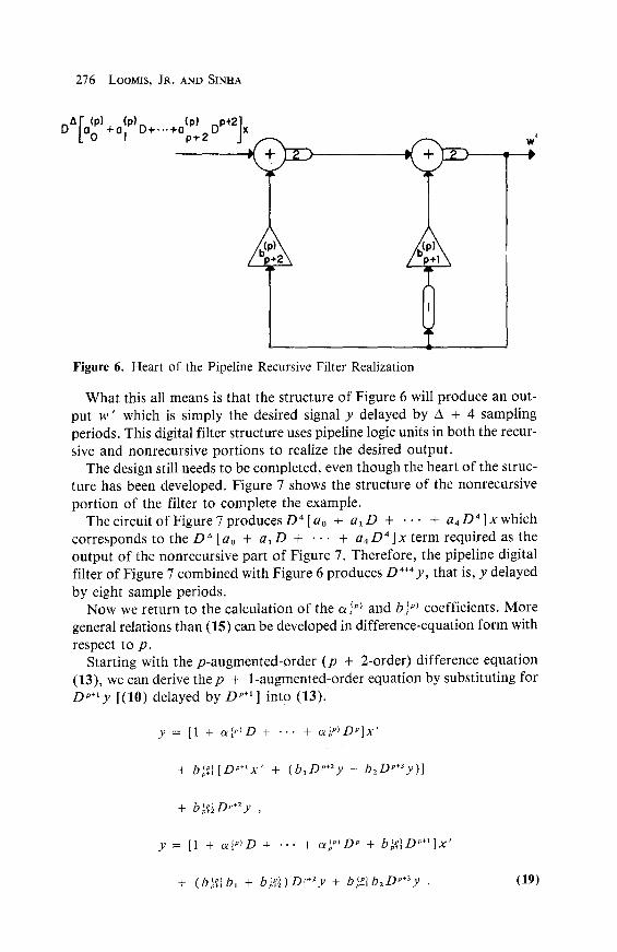
Figure 6. Heart of the Pipeline Recursive Filter Realization

What this all means is that the structure of Figure 6 will produce an output w ' which is simply the desired signal y delayed by A + 4 sampling periods. This digital filter structure uses pipeline logic units in both the recursive and nonrecursive portions to realize the desired output.

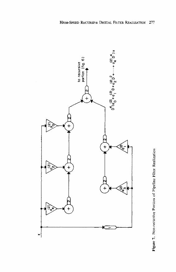
The design still needs to be completed, even though the heart of the structure has been developed. Figure 7 shows the structure of the nonrecursive portion of the filter to complete the example.

The circuit of Figure 7 producesD 4 [ao + a i D + �9 �9 �9 + a 4 D 4 ] x w h i c h

corresponds to the D ~ [ao + a i D + . . . + a4D4]x term required as the output of the nonrecursive part of Figure 7. Therefore, the pipeline digital filter of Figure 7 combined with Figure 6 produces D4+4y, that is, y delayed by eight sample periods.

Now we return to the calculation of the a ~P~ and b) p~ coefficients. More general relations than (15) can be developed in difference-equation form with respect to p.

Starting with the p-augmented-order (p + 2-order) difference equation (13), we can derive the p + 1-augmented-order equation by substituting for D ; + l y [(10) delayed by D p+I ] into (13).

y = [1 + o ~ i " D + " " + o ~ p ) D ~ ] x '

+ b ~ [ D p * ~ x ' + ( b , D ~ § + b2Dp+3Y)]

+ b ~ D ~ ' + 2 y ,

( p ) p + l t y = [1 + o~Ip~D + . . . + o~p~DP + b~+~D ] x

+ ( b ~ b l + b ~ ) D p * 2 y + b~e lb2Dp+3Y �9 (19)

X

L/

"k

S % /

T

Figu

re 7

. N

on-r

ecur

sive

P

orti

on o

f Pi

pelin

e Fi

Tte

r R

ealiz

atio

n

J

\

%

to r

ecur

sive

po

rtio

n (f

ig.

6)

D (a

o+

a2D +...+a 4

u )x

Z ~-..)

'--.I

278 LOOMIS, JR, AND SINHA

F r o m (19) we can see that

~+~ = b~+~ (20a)

b (~*~ ~ b ('~ (20b) p+2 : b.+lb~ + p+2 ,

b(P*~l = b~.~ b~ (20e) p+3

where c~ ~> = 1, b l ~ = b~, and b~ ~ = b2.

Table 1 shows the values o f the coeff icients o f (13) for the values o f p

f r o m 0 th rough 5 as derived f r o m (20). Fur the rmore , mul t ip l ica t ion o f the

p '~-order po lynomia l

c~o ~ + c~I~'D' + . . . + a,(~')D"

by the or iginal

ao + a i D + a 2 D 2

yields the po lynomia l

a~op~ + a ~ D + . . . + .~p~ r~+~ t~ p+2

as shown in (16) and (18). Table 2 shows the values o f a) "> for p f rom 0 th rough 5.

Table l(a). b's f o r p = 0,1 ,..., 5

Coeff ic ient o f D "§ Coeff ic ient o f D "§

b (p) p b~+] ~+~ 0 b~ b2

1 b~ + b~ b~b2

2 b~ + 2b~b2 b~b2 + b~ 3 b~ + 3b~bz + b~ b4b2 + 3b~b~ + b~

4 b~ + 463b2 + 3b~b~ b~b2 + 3b~b~ + b~ 4b~b2 + 3b~b~ 5 b~ + 5b4b2 + 6b~b~ + b~ b~b~ + 3 z

Table l (b) . ~ 's f o r p = 0 ,1 , . . . , 5

p ~0 ~p) alp> cdp) cd,> ~F ~ cd ~

0 1 0 0 0 0 0

1 1 b~ 0 0 0 0

2 1 b~ b~ + b~ 0 0 0 3 1 b~ b~ + b2 b~ + 2b~b~ 0 0 4 l b~ b~ + b2 b~ + 2b~b~ b~ + 3b~b~ + b~ 0 5 1 b~ b~ + b~ b~ + 2b~b~ b~ + 3b~b2 + b~ b s + 4b~b2 + 3b~b~

Tab

le 2

. a

(p~

Coe

ffic

ien

ts o

f E

qu

atio

n (

17)

p a6

"'

aW

a

l"

a~ "~

a

~

a~"'

a~

~ a~

"

0 ao

a

, a2

0

0 0

0 0

1 ao

a~

b,

+

a~

a~b,

0

0 0

0

2 ao

a

ob

t +

a~

a~

(b~

+

b~

) 0

0 0

ao

(b~

+

b~

)

+

atb

t +

a~

a,(

b~

+

b~

)

+ a

zb~

ao

(b]

+

2b~

b2)

ao

(b~

+

b

z)

3 ao

ao

b~

+ a

, +

a~

(bI

+

b2)

+ a

~(b

7

+

2b

~b

z)

0 +

at

b~

+

a~

+ a

~b

, +

a~

(b~

+

b~

) +

a

2(b

~

+

2b

,b2

)

ao

(b~

+

2b

,b~

) a

o(b

~

+

3b~

b2

+

b~

) a

~(b

~

+

bz)

4

ao

ao

b,

+ a

, +

a~

(b~

+

b~

) +

a

~(b

~

+

2b~

b~)

+ a

~(b

~

+

3b~b

2 +

b

~)

+ a

tbj

+ a

2 +

a

z(b

~

+

3b~

b~

+

b~

) +

a2b

~ +

a

~(b

] +

b~

) +

a~

(b~

+

2b

,bz)

ao

(b~

+

b2

) a

o(b

~

+

2b

,b~

) a

o(b

~

+

3b~

b~

+

b~

) a

o(b

] +

4b

~b~

+

3

b~

b~

) a

~(b

~

+

4b~

b~

+

3b

,b~

) 5

ao

ao

b,

+ a

~ +

a~

(b~

+

b~

) +

a,(

b]

+ 2

b~b~

) +

a

~(b

~

+

3b

]b~

+

b

~)

+

a~b~

+

az

+

a~

(b~

+

3b

~b~

+

4b~

) +

a~

b,

+ a

~(b

~

+

b~)

+

a~

(b~

+

2b

~b

~)

d~

U

70

<

0

>

+ a

~(b

~

+ 4

b~b2

+

3b

~b~

Z


DA ( a(~)+ ... + a(pP+]2 D P+ 2 ) x

ko-I

DAf2koy

-

Figure 8. Heart of More General Pipeline Filter Realization

The unique structure of this realization, which differs from conventional realizations of digital filters, is contained in the recursive portion, where the basic feedback loop involving the longest delay passes th roughp + 2 pipeline stages for the realization of a second-order filter. In the example developed, p was 2, causing us to use a fourth-order pipeline filter representation of the original second-order filter.

In general, we assume we have ko-stage pipeline add units and kin-stage pipeline multipliers. The structures of the realization of the feedback portion of the filter would be as shown in Figure 8. Since the maximum delay around the loop must match the p-augmented difference-equation order, we have

p = 2k~ + k m - 2 . (21)

The FIR portion of the filter is shown in general terms in Figure 14. From this figure, it should be clear that

A = [log2(ko) 1 k~ + ko +km

and that the overall delay is therefore

A + 2ko = ~log2(k,) ~ k. + 3ko + /,:~ . (22) ! /

Stability Issues

In the previous section we have seen the general process of realization of a digital filter transfer function using pipeline multiply-add units with delay


2. We have also shown a realization using two-stage multiply-add units. The essence of the technique is to represent a second-order section by means of a (2 + p ) *h-order section of a particular form, where p is determined by the number of stages in the pipeline multiply and add units.

We know from other considerations that the transfer function of the higher- order realization must in fact be the same as the original and therefore must have the same poles and zeros in the z plane. Thus, the operation which transforms (7) into (17) can be thought of in the following way:

( a o + a l z -1 + a2z-2)(1 + a [ " ' z -~ + . . . + o ~ " ~ z - " )

H ' ( z - ' ) = (1 - b l z -~ - b~z2)(1 + a i " ) z -1 + . . . + a ~ " ' z - " ) (23)

a~o p, + a~p~z-~ + . . . + a ~ . A z - . -2 = ( 2 4 )

1 - h c.) . - , , - 1 _ b .+2c~ z - " - 2 , V p + 1 1o

where the coefficients of the a polynomial depend on the original bl and b2 of (5) and (7). These ~ coefficients are governed by (20) and some were tabulated in Table lb. Thus, we raise the order of the denominator, introduc- ingp new poles and corresponding cancelling zeros. These new poles correspond to the roots of

0 = 1 + c ~ i " ~ D + . . . + a ~ " ) D " . ( 2 5 )

The roots of a (D) , of course, are the poles in the z-1 plane and are the reciprocal of the poles in the z plane.

One concern in the realization is that the filter be stable, that is, that it have an impulse response which decays to zero. A sufficient condition for the stability of a digital filter with transfer function H ( z -1 ) is that the poles of H ( z -1 ) in the z -1 plane lie o u t s i d e the unit circle, and that the order of the numerator ( - m ) be less than or equal in magnitude to the order ( - n ) of the denominator. A more familiar sufficient condition is that the poles of the transfer function of z ( H ( z ) ) be i n s i d e the unit circle.

Now, if we start with a stable filter, we would like to be assured that the poles of the augmented-order filter all be outside the unit circle in the z -1 plane. We desire this because, even though the added poles are cancelled by the zeros of ( 1 + a tp) z -1 + �9 �9 �9 + a t"~ z -p ), realization imperfections will prevent exact cancellation and the augmented filter would be unstable.

In order to examine the stability question, we will make use of Jury's stability test [6] as applied to the successively higher-degree denominator polynomials in z as p increases.

We start with the denominator of (5), written as a polynomial in z:

P ( z ) = z 2 - b l z - b2 . (26)

l

m

-I

D k~

x

~ m

'x.

m

rlog2

k ]

leve

ls

I I I

DA

,

(p)

(p)

~p~-

2,

la o

+...

ap

f2U

/

x

ko I

Jog2

kol "

1- ko

+ k m

A

=

Note

= fig

ure

illus

trote

s co

sew

here

p+l

is

inte

ger

mul

tiple

of

k o.

ix9

t-

�9

7 >

Fig

ure

9.

R

eali

zati

on

o

f F

IR

Po

rtio

n

of

Fil

ter


To ensure tha t the original poles of (5) are inside the unit circle and hence tha t the or iginal filter is stable, we app ly Ju ry ' s test with necessary condi t ions:

P ( 1 ) = 1 - b l - be 2> 0 ,

( - I ) ' P ( - 1 ) = 1 + bl - b2 > 0 ,

a n d sufficient condition

!b2! < 1 . (27)

Polynomial: F(z)= z ,-rb I z-b2= 0 Condit ions for Stabi l i ty:

l-bl-b2>O ........... (~) 1+b,-b2>o ........... |

1

; i

/

Figure 10. Condition for Stability of the Original Filter

284 L00MIS, JR. AND SINHA

Hence, for this second-order digital filter to be stable, the values o f bl and b2 must be in the shaded area as shown in Figure 10. Note that this is the case when p = 0, i.e., no augmentat ion.

Now, assuming that the original filter transfer funct ion (5) is stable, i.e., (27) is satisfied, it is desirable to determine conditions to assure stability o f the new p poles in t roduced into the system when the transfer funct ion is p- augmented. For p = 1, the new polynomial int roduced in the numera tor and denomina tor is

F ( z ) = z + b l �9

Applying Jury ' s test, conditions for stability are

F ( 1 ) = 1 + bl > 0 ,

( - 1 ) " F ( - 1 ) = 1 - b~ > 0 .

(28)

(29) This condit ion, Jbll < 1, is shown graphically in Figure 11. Similarly, for p = 2, the added polynomial is

F ( z ) = z 2 + b l z + ( b ~ + b 2 ) . (30)

Polynomial: F ( z ) = z +b 1 = 0

Conditions for Stability:

1+ b l>O . . . . . . . . . . . . C~)

1 - b l > O . . . . . . . . . . . . ( ~

I

I I-1 I

Figure 11. Condition for Stability of the Augmented Filter: p = 1


Jury ' s test gives condi t ions for stable roots. The necessary condi t ions are

F ( 1 ) = 1 + b1 + (b~ + b2) > 0 ,

( - ] ) ~ = 1 - b , + ( b ~, + b=) > 0 ,

and the sufficient condition is

]b 2 + b21 < 1 . (31)

The region defined by condi t ions (31) is shown graphically in Figure 12.

Polynomial= F(z)= z2+ b 1 z + ( b12+ b2 ) Conditions for Stability=

1+bl+(b2+b2) >0 . . . . . . . . . . . . (~

l§ b~+b 2 >0 . . . . . . . . . . . . (~) < , . . . . . . . . . . . .

bl L



Finally, for p --- 3,

F ( z ) = z ~ + b , z 2 + (b} + b~)z + (b 3 + 2b ,b2) ,

and the conditions for stable poles are (Figure 13):

F(1) = i + b, + (b, 2 + b2) + (b 3 + 2b lb2) > 0 ,

( - l ) n F ( - l ) = I - b~ + (b~ + b2) - (b~ + 2b ,b2) > 0 ,

Ib 3 + 261b21 < I ,

l (b~ + 2b ,b2) ~ - 11 > I b , ( b 3, + 2 b , b 2 ) - (b} + b2)l �9

Polynomial: F(z)= z3+blZ2+ (b2+b 2) z +(bSi+2b Ib 2) Conditions for Stability

2 3 l+bl+(bl+b2)+(bl +261b2) > 0 ................. (~

, - b , + l b ~ b , ~ - c : , + 2 b , ~ _ _ _ _ >o . . . . . . . . . . . . . . . . |

I b~"2b,': '~l <~ . . . . . . . . . . . . . . . . . . . . . . | 3 2 D]'3+2bl 2

bl h.~

(32)



This procedure can be continued for higher values of p; in fact general stability tests based on Jury's test have been developed [6]. Unfortunately, those tests are cumbersome to apply.

Instead, let us take another approach. From Figures 10-13 it may be observed that as the value of p increases,

the area of stability (the shaded areas in the figures) tends to increase. It has been seen graphically that as p increases, the stable region approaches the original shaded area for p = 0, i.e., Figure 10. This leads to the obvious conjecture t]~at all stable filters have a stable augmented filter for some large enough p.

We will follow the procedure suggested by Voelcker [7] for block filters to show that for a large value of augmentation, p, the pipelined version of the original filter will always be stable, provided that the original second- order filter is stable. This is a very important and useful conclusion and implies that an augmented stable realization is always possible if the original transfer function is stable. The proof of this fact follows

Since the process of augmentation implies multiplying the numerator and denominator by the same polynomial, the original transfer function may be equated to the augmented transfer function as

N ( z ) N ( z ) ( o ~ W + o ~ W Z -~ + . . . + ~ W z - ' )

1 - b x z -1 - b ~ z -z (p -1 1 - Z -~'§ (h~,~,+, + b , A z )

where N( z ) is the numerator of the original transfer function. Denoting the denominator of the original transfer function as D (z), since this original filter is stable, the roots o f D (z) are inside the unit circle. Figure 14(a) shows the original filter, where H , (z) is a pole-only function representing the denominator, ( 1 /D ( z ) ) of the original filter.

The process of augmenting the difference equations suggests building the filter as shown in Figure 14(b), where

o ~ ( z ) -- c~g ~ + c ~ ' z -~ + . . . + o ~ ? ' z - "

and

G ( Z ) --- h~p~ + b ~ " 1 " - 1 p + l p+2 A,

Thus

H~,(z) - 1 _ a ( z ) ( 3 3 ) D ( z ) 1 - z - ( ~ G ( z )

Hence, the nonrecursive transfer function c~ (z) may be written as

o ~ ( z ) = H v ( Z ) - Z -C'§ G ( Z ) (34) D ( Z )

288 L 0 0 M I S , JR . AND SINHA

X(Z) J N(z) H (Z)=D-~z)

(o)

Y(z)

x (z)~

Hp(Z) s . . . . . . . . . . . . . . . . . . . . . . . . . . . . . . . . . . . !

!

_ ~Y(z)

. . . . . . . . . . . . . . . . . . . . . . . . . . . . . . . .

( b )

N(z)

Figure 14. (a) Original Transfer Function; (b) Equivalent Augmented Transfer Function

Since kip (z) is a pole-only transfer function,

H , ( z ) = (ii )_1 1 - z i / z

i=1

2 al

= ~ 1 ---Z,/Z " i=1

Taking the inverse t rans form

2

h p ( n ) = ~ alz7 i=1

Since zl and z2 are the initial poles, they are inside the unit circle. Hence hp ( n ) is an infinite sequence decreasing in magnitude. I f the sequence is trun- cated at the ( p + 1 ) term, the remaining por t ion o f the sequence

H I G H - S P E E D RECURSIVE DIGITAL FILTER REALIZATION 2 8 9

h p ( n ) = ~ a l z 7 n = 0,1 , . . . ,p i=1

0 otherwise

Taking the z-transform

P

Jq,(z) = ]~ L( , , ) z T M

n=0

p 2

E aiz z-~ n=0 i=1

"= n=0

i=l al 1 - (Z~/Z)

Thus,

2 2 al at (Z l /Z) .+1

1 - (Ze/Z) - E ~-_ i=l i=1

2 aezf +1

~ p ( z ) = H , ( z ) - z -'p*l' ~ 1 2 - (~ , / z ) i=1

(35)

Comparing (34) and (35)and, since/-~r(z) is a finite-impulse-response transfer function, equating/-)p (z) and o~ ( z ) ,

Thus

2 a ~ z f +1 G ( z ) _ ~

D ( z ) 1 --- ~-,/z i=1

~a,zV I D ( z ) G ( z ) = -l ~ Z Z z

i=1

(36)

The intent of this procedure is to prove that for some high value of p , all roots of o~ (z) are inside the unit circle in the z-domain. From (33),

D ( Z ) O l ( Z ) = 1 - Z-C~+llG(z) . (37)

Since D (z) is the denominator of the original transfer function, all roots

290 LooM~s, JR. A~'~D SINHA

of D ( z ) are inside the unit circle. Hence all roots of c~ (z) are also inside if and only if all roots of the right-hand expression of (37) are inside the unit circle. To do this, let tilde (-) denote the result of the mapping z -~ -- z i.e., f ( z ) = f ( z -~) and ~ (z ) is defined as

d ( z ) = 1 - z ' ~ + ' d ( z ) = ,O ( z )~ ( z ) . (38)

All roots o f / 3 (Z) are exterior (outside the unit circle). Hence, all roots of c~ (z ) are exterior if all roots of /~ (z) are exterior. To prove this, Rouche 's theorem is used, which states that: " I f f ( z ) and g ( z ) are analytic inside and on a closed contour C, and !g ( z ) l < I f ( z ) ! on C, then f ( z ) and f ( z ) + g ( z ) have the same number of zeroes inside C . " Clearly, A in (38) is analytic within and on the unit circle. The constant " 1 " has no interior zeroes. Hence A (z ) wilt have no interior zeroes if, on the unit circle,

IZ ~p+~G(z) I < 1, z = e ~~ �9 (39)

F r o m ( 3 6 ) ,

~z=e J~ 1 - - s ,~ i - i

(40)

However, I z,I < 1 for all i because these are poles of the original filter. Thus, for some value of p greater than some critical value, equation (40) will be satisfied. Note that (,10) may be satisfied for smaller value of p also.

From the above discussion, it may be concluded that for some high value of augmentation, it is always possible to ensure that c~ (z ) has roots inside the unit circle. Since these roots are the new additional poles of the augmented system, the new high-order transfer function would be stable.

As a result of this fact, the following design method is suggested. We assume that the designer is given a stable recursive digital filter transfer

function H ( z ) and a desired sampling (clock) rate of operation, f , .

1. Find k~-stage pipeline multiply and k~-stage pipeline add units that wilt operate at clock frequency f , .

2. Factor H ( z ) into f ( f - 1 if n is odd) second-order (and if n is odd, at most one first-order) transfer functions.

H ( z ) = H , ( z ) H ~ ( z ) ... H A z ) ,

where f = [ n / 2 ~ . 3. For each H , ( z ) , i = 1, 2 ,.. . , f. Realize H~(Z) as follows:

a. S e t p = 2k~ + k,~ - 2. b. Determine the polynomial 1 h ~,~ _ ~,,§ _ b~z -p-2 = B , ( z -~ ) . c. Solve for the roots of B~ (z "~) = 0.


d. I f all roo t s o f Bp ( z -1 ) = 0 are ou t s ide the uni t circle, go to e; o ther -

wise set p = p + 1 a n d r e t u r n to s tep b.

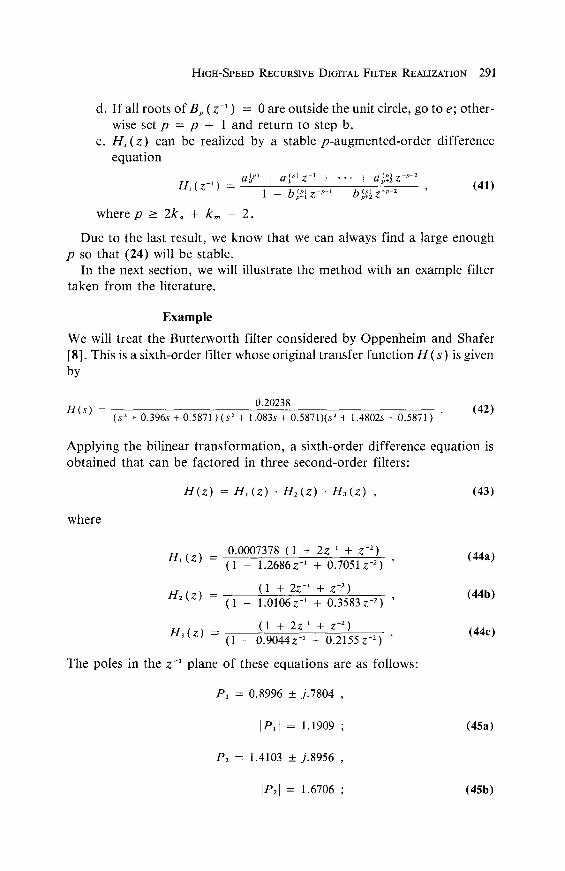
e. H i ( z ) can be rea l ized by a s table p - a u g m e n t e d - o r d e r d i f f e r e n c e

e q u a t i o n

a~o~ ~ + a I ~ z - ' + . . . + a~+~z -~-~ H, ( z -I ) = , (41)

1 h (p) (p) -p-: - - c , p + l Z - p - 1 - - b p + 2 Z

where p _> 2ko + k , - 2.

D u e to the last resul t , we k n o w tha t we can a lways f ind a large e n o u g h

p so tha t (24) will be s table .

In the nex t sec t ion , we will i l lus t ra te the m e t h o d wi th an e x a m p l e f i l ter

t a k e n f r o m the l i t e ra tu re .

E x a m p l e

W e will t rea t the B u t t e r w o r t h f i l ter c o n s i d e r e d by O p p e n h e i m a n d S h a r e r

[8]. Th is is a s ix th -o rde r f i l ter w h o s e o r ig ina l t r ans f e r f u n c t i o n H ( s ) is g iven

by

0.20238 H ( s ) = (42)

(s2+ 0.396s + 0.5871)(s 2 + 1.083s + 0.5871)(s 2 + 1.4802s + 0.5871)

A p p l y i n g the b i l inea r t r a n s f o r m a t i o n , a s i x th -o rde r d i f f e r e n c e e q u a t i o n is

o b t a i n e d tha t can be f a c t o r e d in th ree s e c o n d - o r d e r f i l ters :

H ( z ) = H , ( z ) . H 2 ( z ) . H 3 ( z ) , (43)

w h e r e

H,(z ) = 0 . 0 0 0 7 3 7 8 (1 + 2 z - ' + z -2) ( 4 4 a ) (1 - 1.2686z -1 + 0.7051z -z) '

H 2 ( z ) = (1 + 2Z -~ + Z -2)

(1 - 1.O106z -1 + 0.3583z -2) '

H3 (z ) = (1 + 2z -~ + z -2)

(1 - 0.9044z -~ + 0.2155z -2)

T h e po les in t he z - ' p l ane o f these e q u a t i o n s are as fo l lows :

( 4 4 b )

( 4 4 c )

P, = 0.8996 • j .7804 ,

IP,] = 1.1909 ; (45a)

P2 = 1.4103 • j .8956 ,

[P2] = 1.6706 ; (45b)


P3 = 2.0984 • j.4870 ,

IP31 = 2.1542 . (45c)

Thus all three of the factoring second-order transfer functions are stable. p-augmented-order difference equations of the form of (16) were derived

for each of the three sections, for values o f p from 1 through 5. H , and H2 were unstable for p = 1 and stable for all values of p from 2 through 5. H3 was stable for all values of p from 1 through 5.

If we had a two-stage adder and a two-stage multiplier, (21) would yield a p of 4, which for our example adds stable poles to each section. The general structure of each of the second-order (four-augmented) sections would be as shown in Figure 15.

Finally, the values for the coefficient of each of the multipliers would be as shown in Table 3.

Note that the a <4) coefficient for the first section are all on the order of 0.001 in magnitude. These coefficients could easily be computed to more significant figures, although realization of more significant figures in the coefficient of an actual filter would require either scaling or the use of a floating- point number system.

This example shows how an IIR filter can be realized using high-rate pipeline modules, with the ultimate objective of achieving a higher sample rate than possible with nonpipelined multiplier and adders.

Table 3. Coefficient of Filter Section in Figure 15 to Realize Sixth-Order Butterworth Filter

a~ 4) a~ n') a2c4) a3~4) a~ 4, as{ 4, a6 (4) as(41 a6(41

H , (z -~) 0.0007 0.0023 0.0031 0.0023 0.0008 -0.0003 -0.0002 -0,5804 0.2236

H2 (z -1) 1.0 3.0106 3.6842 2.6446 1.3525 0.4552 0.0736 -0,0359 -0.0264

H3(z -1) 1.0 2.9044 3.4112 2.4592 1.4890 0.7233 0.1867 0.0934 -0.0402

S u m m a r y and Conclus ions

In this paper we have developed a method for applying pipeline techniques to the design of high-speed recursive digital filters. Using these techniques, recursive digital filters operating at rates hithert O impossible can be designed. The general structure of the filter and the method for calculating the multiplier coefficients have been presented. The stability of the resulting realization has been investigated and a technique for ascertaining the stability of the realization has been presented.

A significant example taken from the literature has illustrated the technique and demonstrated the existence of a stable high-rate pipeline realization of a practically useful filter.

XA

"k

7~ Y

Bos

ic

Pip

elin

e M

odul

es

2 -s

tage

mul

tiply

2-

sta

ge

8- s

tage

by

4

adde

r de

lay

Fig

ure

15.

Sixt

h-O

rder

Pip

elin

e R

eali

zati

on o

f Se

cond

-Ord

er R

ecur

sive

Filt

er

Y \/

\

6~

7~

N

7~

t~


References

[1] Loomis, H. H. Jr., TheMaximum Rate Accumulator, IEEE Tec. EC-15, 4 (1966), 628-639.

[2] Chen, T. C., Overlap and Pipeline Processing, Introduction to Computer Ar- chitecture, H. Stone, editor, Science Research Associate, Chicago, Chapter 9.

[3] Cray Research, Inc., Cray-1 Hardware Reference Manual, Cray Research Publica- tion No. 2240004, Rev. E, 1979.

[4] Soderstrand, M. A. and Fields, E. L., A High Speed Low-Cost Recursive Digital Filter Using Residue Number Arithmetic, Proc. IEEE (1977).

[5] Sinha, B., Pipelined Finite State Machine Architecture Applied to Digital Filters, Ph.D. Dissertation, University of California, Davis, CA, September 1983.

[6] Nagrath, I. J. and Gopal, M., Control Systems Engineering, Halsted, Wiley, 1982. [7] Voelcker, H. B. and Hartquest, E. E., Digital Filtering Via Block Recursion,

IEEE Transactions on Audio and Electroacoustics (1970). [8] Oppenheim, A. and Shafer, R., Digital Signal Processing, Prentice-Hall,

Englewood Cliffs, N J, 1975.

High-speed recursive digital filter realization

Documents

Transcript of High-speed recursive digital filter realization