A study of the recursive filter for computing scalar

eddy covariances

Mikhail S. Pekour *, Marvin L. Wesely, David R. Cook, Timothy J. Martin

Environmental Research Division, Argonne National Laboratory, Argonne, IL 60439-4843, USA

Received 19 February 2004; received in revised form 11 November 2004; accepted 4 December 2004

Abstract

Values of turbulent fluxes in the atmospheric surface layer obtained with block averaging and with recursive filtering showed

consistent differences during a 4-day experiment conducted over grassland in central Kansas. Analysis of the direct and indirect

impacts of recursive filtering on the calculated fluxes showed that flux values can be affected significantly by mismatched filtering in

different channels, unsuitable filter initialization, a poor choice of coordinate rotation technique, or a combination of these.

# 2005 Elsevier B.V. All rights reserved.

Keywords: Eddy covariance; Recursive filtering; Atmospheric turbulent fluxes

www.elsevier.com/locate/agrformet

Agricultural and Forest Meteorology 136 (2006) 101–107

1. Introduction

The current study grew from an investigation of

unexpected results from a short field campaign designed

to compare different flux measurement systems as a part

of an AmeriFlux intercomparison at the Walnut River

Watershed site in southeastern Kansas in May 2001.

Among other data conditioning and quality control

procedures, we evaluated possible flux loss from

recursive filtering by comparing: (1) 30 min flux

estimates obtained by block averaging and (2) flux

estimates calculated with recursive filters applied with

various effective time constants. Under reasonably

stationary conditions, we expected recursive filter

estimates to approach the block-averaged value from

below as the effective time constants are increased.

However, we found that recursive filtering produced

* Corresponding author. Present address: Atmospheric Science and

Global Change Division, Pacific Northwest National Laboratory,

Richland, WA 99352, USA. Tel.: +1 509 375 2470;

fax: +1 509 372 6168.

E-mail address: mikhail.pekour@pnl.gov (M.S. Pekour).

0168-1923/$ – see front matter # 2005 Elsevier B.V. All rights reserved.

doi:10.1016/j.agrformet.2004.12.011

flux densities 5–10% lower than block averaging, even

for very long effective time constants.

Recursive filtering is a well-known technique that has

been broadly used. However, it has several inherent

problems that tend to be overlooked. Although current

common opinion does not favor recursive filtering, the

procedure is still in use (Kruijt et al., 2004) and it is

indispensable for applications such as real-time mea-

surements made from a moving platform (aircraft, vessel,

car, etc.).

Adequate accounting for the low frequency contribu-

tion to fluxes is important for long-term flux measure-

ments (e.g., Sakai et al., 2001; Massman and Lee, 2002;

Kruijt et al., 2004). In this context, we look to a case study

of artifact flux underestimation to reveal potential

sources of significant errors in long-term flux studies.

2. Experimental data

We deployed two eddy covariance systems at the

AmeriFlux Walnut River Watershed site in southeastern

Kansas on 15–17 May, 2001. The major objective of the

campaign was to compare several flux measuring

M.S. Pekour et al. / Agricultural and Forest Meteorology 136 (2006) 101–107102

systems within the AmeriFlux framework; here, we use

the data collected as convenient material to illustrate the

problem, our approach, and the results.

The eddy covariance systems used sonic anem-

ometers and open-path infrared gas analyzers for fast

synchronous measurements of wind, temperature, and

densities of water vapor and carbon dioxide. The sonic

anemometers used were from Gill Instruments (http://

www.gill.co.uk1), Omnidirectional Model R3. One

infrared gas analyzer was an ATDD (Atmospheric

Turbulence and Diffusion Division, http://www.atdd.-

noaa.gov2) instrument, and the other was a LI-7500 (LI-

COR Environmental, http://www.licor.com/env/3)

instrument. The two systems were set up side-by-side

and 4 m apart, with sensors 4 m above ground level, in a

grazed, mixed-grass field with a slight slope to the south

and good fetch in all directions.

Raw data recorded with a 20 Hz acquisition rate

were saved in 30 min periods. The data were screened

for spikes, excessive noise, and unusual spectral shapes;

30 min data sets with unwanted characteristics were

excluded from subsequent analyses.

Data analyses included estimation of heat, moisture,

and carbon dioxide fluxes by using 30 min block

averages or a recursive filter with effective time

constants ranging from 50 to 800 s.

The recursive filter was implemented in the form:

xi ¼ xi þ e�D=tðxi�1 � xiÞ (1)

x0i ¼ xi � xi: (2)

Here, xi is the local mean (low-frequency component),

x0 is the departure from the local mean (fluctuating part),

D is the sampling interval (0.05 s), and t is the effective

time constant.

Traditional two-dimensional coordinate rotations

were performed to force means of transverse and vertical

wind components to zero. For block averaging, we used

rotation to bring the mean of vertical wind to zero; for

recursive filtering, however, the mean of the fluctuating

part of the vertical wind was forced to zero. When the

vertical wind is decomposed into mean w and fluctuating

w0 parts by high-pass filtering, the mean value of either

portion is not necessarily equal to zero. The meanvalue of

any one of three vertical wind variables (w; w; or w0)might be zeroed by coordinate rotation; this choice can

1 Gill Instruments.2 Atmospheric Turbulence and Diffusion Division.3 LI-COR Environmental.

have great impact on subsequent flux calculations, as will

be shown later.

In the calculation of covariances, special attention

was given to choosing the proper time delay between

data streams from different sensors. Time delays can be

caused by differences in the processing time of digital

sensors (e.g., Zeller et al., 2001), spatial separation of

the sensors, etc. We used the maximum of the

corresponding covariance function as a pointer to the

appropriate time lag. For the Gill–ATDD combination,

the sonic data had to be advanced by one digitization

time step (+0.05 s), while for the Gill–LI-COR

combination, the sonic data had to be delayed by four

steps (�0.2 s). The ATDD sensor is an analog device

that has virtually no time lag between measurement and

data output; the Gill R3 sonic anemometer has a time

delay of about 0.05 s, which explains the 0.05 s lag for

the Gill–ATDD pair. The LI-COR sensor has an

unavoidable internal delay of 0.230 s; it was pro-

grammed for an additional 0.019 s delay to bring the

total delay closer (within 0.02 s) to an integer number of

digitization steps.

Net radiation data were obtained from a REBS

(Radiation and Energy Balance Systems, Inc., Seattle,

Washington) Q*7.1 net radiometer, and soil heat flow

was obtained from an array of five sets of REBS STP-1

soil temperature probes, SMP-1 soil moisture probes,

and HFT-3 heat flow plates. Further details of the

eddy covariance system and other instrumentation

are on line at http://www.atmos.anl.gov/ABLE/instru-

ments.html4.

After spectral corrections for limited frequency

response and space separation of the sensors (Massman,

2000; Rannik, 2001), the sum of sensible and latent heat

fluxes, H + lE, found by 30 min block averaging, was

sufficiently large to close the energy balance for both

systems (Fig. 1). These flux estimates were consistently

larger than the fluxes computed with the recursive

filters. The differences during the daytime were usually

largest for water vapor, intermediate for carbon dioxide,

and smallest for heat. The differences for the recursive

filter were typically 10–18% with a 50 s time constant

and 5–10% with an 800 s time constant. An example of

the average difference between sensible heat flux

estimates made by using block averaging and recursive

filters is shown in Fig. 2, line 1.

In general, an energy balance closure test may not be

the best evaluation of the performance of an eddy

covariance system (e.g. Twine et al., 2000); it involves

4 Argonne Boundary Layer Experiments.

M.S. Pekour et al. / Agricultural and Forest Meteorology 136 (2006) 101–107 103

Fig. 1. Daytime energy balance components with 30 min block

averaging for the eddy fluxes of sensible and latent heat, H + lE,

vs. the sum of net radiation and soil heat flux, Rn + G, for two systems,

Gill–ATDD (+) and Gill–LI-COR (�). The dashed lines show coin-

cidence and �15% difference.

data from several different sensors, each with errors and

limitations. Even more important, there are large

differences in footprints among the sensors, from several

square meters for the soil heat flow and net radiation

measurements, to tens of thousands of square meters for

eddy covariance fluxes. However, in our case of fairly

stationary conditions and rather uniform terrain, we can

take the result of the energy balance test as reasonable

proof that block-averaged fluxes may be used as a valid

Fig. 2. Relative flux loss associated with recursive filter application.

Line 1 (�—�) is the average difference (‘‘loss’’) in daytime sensible

heat flux estimates for recursive filtering as compared to block

averaging, expressed as percentage of block-averaged values. Line

2 (+—+) is an estimate of the effect of high-pass filtering [attenuation

factor b(t) as in Eq. (19)] on sensible heat flux under neutral

conditions for the Kaimal cospectrum, with mean wind speed of

4 m s�1 and height of 4 m above the ground. Line 3 (D—D) is the

average difference of sensible heat flux estimates made with the same

recursive filters and two coordinates rotation schemes, w ¼ 0 and

w0 ¼ 0, expressed as percentage of block-averaged values.

approximation to ‘‘true’’values in comparisons and in the

demonstration of relative flux lost.

In the remainder of this paper, we do not apply

spectral corrections to any flux estimate. This is

because: (a) corrections due to sensors (dimensions,

separation, time response, etc.) are the same for all

filtering methods; (b) the difference between the

spectral correction for block averaging and for recursive

filtering becomes negligible with sufficiently long time

constants; (c) we wish to avoid involving in the

discussion another complex, still unresolved matter

(i.e., spectral corrections) that would unnecessarily

complicate and obscure the results.

3. Discussion

Since the effects of the 800 s recursive filter are

roughly equivalent to block averaging over a period of

40 min, some mechanisms besides simple filter attenua-

tion must be responsible for the additional flux loss. We

consider three factors associated with filtering as

possible causes: (a) direct recursive filter effects, (b)

unmatched filter initialization, and (c) distortion of

computed vertical flux resulting from improper coordi-

nate rotation.

3.1. Direct filter effects

Filter impact can be described by using the approach

of Kristensen (1998) (see also Horst, 2000, and

references herein). Let wðtÞ and s(t) be the vertical

velocity component and the scalar, respectively; then,

recursive high-pass filtering with a time constant t can

be expressed as:

w0ðtÞ ¼1

t1

Z t

0

wðt � t1Þ exp

�� t1

t1

�dt1; (3)

s0ðtÞ ¼1

t2

Z t

0

sðt � t2Þ exp

�� t2

t2

�dt2; (4)

w0ðtÞ ¼ wðtÞ � w0ðtÞ; (5)

s0ðtÞ ¼ sðtÞ � s0ðtÞ; (6)

where w0ðtÞ and s0(t) are local means, and w0ðtÞ and s0(t)are fluctuations (deviations from local means). Then,

the covariance of fluctuating parts for a series of length

T becomes:

w0s0 ¼ wsþ w0s0 � ws0 � w0s; (7)

where

M.S. Pekour et al. / Agricultural and Forest Meteorology 136 (2006) 101–107104

w0s0 ¼Z T

0

dt1

t1

exp

�� t1

t1

�Z T

0

dt2t2

exp

�� t2

t2

�wðt � t1Þsðt � t2Þ

¼Z T

0

dt1

t1

exp

�� t1

t1

�Z T

0

dt2t2

exp

�� t2

t2

�Z þ1�1

GðvÞ expðivðt2 � t1ÞÞ dv; (8)

w0s ¼Z T

0

dt1t1

exp

�� t1

t1

�Z þ1�1

GðvÞ expð�ivt1Þ dv; (9)

ws0 ¼Z T

0

dt2t2

exp

�� t2

t2

�Z þ1�1

GðvÞ expðivt2Þ dv; (10)

and G(v) = Co(v) + iQ(v) is the complex cross spec-

trum, with Co(v) and Q(v) being the cospectrum and

quadrature spectrum, respectively. The last two terms

on the right-hand side of (7) represent so-called Leo-

nard fluxes, which are not equal to zero in this case,

because filtering does not obey Reynolds averaging

rules.

After integration over t1 and t2, and using standard

symmetry considerations, we get:

w0s0 ¼Z þ1�1

ðR1R2 �I1I2ÞCoðvÞ � ðR1I2þR2I1ÞQðvÞð1þ ðvt1Þ2Þð1þ ðvtÞ2Þ

dv;

(11)

w0s ¼Z þ1�1

R1CoðvÞ � I1QðvÞð1þ ðvt1Þ2Þ

dv; (12)

ws0 ¼Z þ1�1

R2CoðvÞ � I2QðvÞð1þ ðvt2Þ2Þ

dv; (13)

where

R1 ¼ 1� exp

�� T

t1

�cosðvTÞ

þ exp

�� T

t1

�vt1 sinðvTÞ; (14)

R2 ¼ 1� exp

�� T

t2

�cosðvTÞ

þ exp

�� T

t2

�vt2 sinðvTÞ; (15)

I1 ¼ exp

�� T

t1

�sinðvTÞ � vt1

þ exp

�� T

t1

�vt1 cosðvTÞ; (16)

I2 ¼ �exp

�� T

t2

�sinðvTÞ � vt2

þ exp

�� T

t2

�vt2 cosðvTÞ: (17)

Note that no imaginary part is left in (11)–(17); all of the

values are real.

In the simplest case, with a sufficiently long series

T� t and with the same filter used on both variables

(t1 = t2 = t), Eq. (7), after substitution of (11)–(17) into

(8)–(10), reverts to the well-known high-pass filter

expression:

w0s0 ¼ ws�Z þ1�1

CoðvÞ1þ ðvtÞ2

dv: (18)

To illustrate the influence of high-pass filtering, we

calculated attenuation factor:

bðtÞ ¼ ws� w0s0

ws(19)

against filter time constant for sensible heat flux under

ordinary conditions (wind speed of 4 m s�1 and height

of 4 m above the ground) by using the Kaimal cospec-

trum of temperature and vertical wind for neutral

stratification (Fig. 2, line 2). Low-frequency attenuation

seems to be negligible, for practical purposes, at less

than 1% for t � 200 s.

In the case of limited series length, when condition

T� t is no longer valid, we get:

M.S. Pekour et al. / Agricultural and Forest Meteorology 136 (2006) 101–107 105

w0s0 ¼ ws

�Z þ1�1

1þ 2 exp

�� T

t

�vt sinðvTÞ � exp

�� 2 T

t

�1þ ðvtÞ2

CoðvÞ dv: (20)

Note that (20) does not depend on the quadrature

spectrum. The function:

Fðv; tÞ ¼2 exp

�� T

t

�vt sinðvTÞ � exp

�� 2 T

t

�1þ ðvtÞ2

(21)

is plotted in Fig. 3 for a half-hour series (T = 1800 s) and

three filter time constants. This function determines the

deviation of filter transfer function from that for a

simple high-pass filter due to ‘‘border effects.’’ This

deviation seems to be negligible for Tt� 5 in the prac-

tical frequency range. This condition can be used to

determine the maximum value of the time constant.

In the case of different filters (t1 6¼ t2) but a

sufficiently long series (T� t), Eq. (7) becomes:

w0s0 ¼ ws�Z þ1�1

ðv2ðt21 þ t2

2Þ þ ð1� v2t1t2ÞÞCoðvÞ þ v3t1t2ðt2 � t1ÞQðvÞð1þ ðvt1Þ2Þð1þ ðvt2Þ2Þ

dv: (22)

The term that contains the quadrature spectrum

describes the so-called out-of-phase corruption; in

other words, two signals that experience different filter

time delays introduce an additional frequency-depen-

dent time lag that leads to underestimation of

covariance.

Fig. 3. ‘‘Border effect’’ function F(v,t) [Eq. (21)] calculated for a

series length of 1800 s and three filter time constants. The angular

frequency v (in radians) has been converted into natural frequency

f = v/2p (in Hz).

Because little is known about the quadrature spectra

of the vertical wind and scalars, it may be instructive to

look at the ratio D(a,t1) of coefficients to Q(v) and

Co(v) in (22):

Dða; t1Þ ¼aða� 1Þv3t3

1

1þ v2t21ða2 � aþ 1Þ ; (23)

where

a ¼ t2

t1

: (24)

Fig. 4 shows the ratio D(a, t1) for several values of

a and filter time constant t1. The absolute value of

the quadrature spectrum is usually assumed to be

lower than the cospectrum by several orders of

magnitude. However, Fig. 4 shows that at frequencies

above 0.5 Hz the contribution from the quadrature

spectrum might become significant because of the v3

multiplier. One important conclusion is that if any of

the sensors has internal high-pass filtering of any kind

(electronic, spatial, digital, recursive, etc.), the impact

of possible phase corruption must be assessed in the

analysis.

3.2. Filter initialization

A recursive filter needs to be initialized at the

beginning of a data series with some mean value.

Fig. 4. Ratio D(a,t) [Eq. (23)] for three different values of t and three

values of a: thick solid line, a = 10; thin solid line, a = 5; dashed line,

a = 2. The angular frequency v (in radians) has been converted into

natural frequency f = v/2p (in Hz).

M.S. Pekour et al. / Agricultural and Forest Meteorology 136 (2006) 101–107106

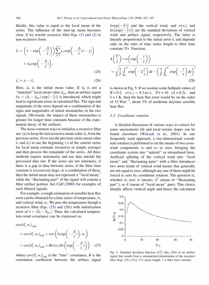
Fig. 5. Standard deviation function A Tt

� �(Eq. (28)) of an artifact

signal that results from a mismatched initialization of the recursive

filter (Eqs. (25)–(27)). T is series length, t is filter time constant.

Ideally, this value is equal to the local mean of the

series. The influence of the start-up mean becomes

clear, if we rewrite recursive filter Eqs. (1) and (2) in

non-recursive form:

xi ¼�

1� exp

��D

t

��Xj¼i

j¼1

x j exp

��D

tði� jÞ

�

þ x0 exp

��D

ti

�;

(25)

x0i ¼ xi � xi: (26)

Here, x0 is the initial mean value. If x0 is not a

‘‘matched’’ local mean value xloc, then an artifact signal

dxi ¼ ðx0 � xlocÞ exp � Dt

i� �

is introduced, which might

lead to significant errors in calculated flux. The sign and

magnitude of the error depend on a combination of the

signs and magnitudes of initial mismatches in the two

signals. Obviously, the impact of these mismatches is

greater for longer time constants because of the expo-

nential decay of the artifacts.

The most common ways to initialize a recursive filter

are: (a) to keep the last recursive mean value xN from the

previous series, (b) to use the previous series mean value

x, and (c) to use the beginning t s of the current series

for local mean estimate (recursive or simple average)

and then process the remainder of the series. All three

methods require stationarity and use data outside the

processed data run. If the series are not stationary, if

there is a gap in data between series, if the filter time

constant is excessively large, or a combination of these,

then the initial mean may not represent a ‘‘local mean,’’

while the ‘‘fluctuating part’’ of the signal will contain a

filter artifact portion. See Culf (2000) for examples of

such filtered signals.

For example, a rough estimation of sensible heat flux

error can be obtained for a time series of temperature, ui,

and vertical wind, wi. We pass the temperature though a

recursive filter (Eqs. (25) and (26)) with initialization

error of d ¼ ðu0 � ulocÞ. Then, the calculated tempera-

ture-wind covariance can be expressed as:

covðu0i;wiÞcalc

¼ covðu0i;wiÞreal þ cov

�d exp

��D

ti

�;wi

�

¼ covðu0i;wiÞreal þ RsðwiÞds�

exp

��D

ti

��(27)

where covðu0i;wiÞreal is the ‘‘true’’ covariance, R is the

correlation coefficient between the artifact signal

d exp � Dt

i� �

and the vertical wind, and sðwiÞ and

ds exp � Dt

i� �� �

are the standard deviations of vertical

wind and artifact signal, respectively. The latter is

linearly proportional to the initial error d, and depends

only on the ratio of time series length to filter time

constant T/t. Function,

A

�T

t

�¼s

�exp

�� t

t

��

¼

ffiffiffiffiffiffiffiffiffiffiffiffiffiffiffiffiffiffiffiffiffiffiffiffiffiffiffiffiffiffiffiffiffiffiffiffiffiffiffiffiffiffiffiffiffiffiffiffiffiffiffiffiffiffiffiffiffiffiffiffiffiffiffiffiffiffiffiffiffiffiffiffiffiffiffiffiffiffiffiffiffiffiffiffiffiffiffiffiffiffiffiffiffiffiffiffi1

T

Z T

0

exp

��2

t

t

�dt �

�1

T

Z T

0

exp

�� t

t

�dt

�2s

(28)

is shown in Fig. 5. If we assume some ballpark values of

R = 0.2, sðwiÞ ¼ 0:3 m=s, T/t = 10 (A = 0.2), and

d = 1 K, then the heat flux error would be on the order

of 15 Wm�2, about 5% of moderate daytime sensible

heat flux.

3.3. Coordinate rotation

A detailed discussion of various ways to correct for

sonic anemometer tilt and local terrain slopes can be

found elsewhere (Wilczak et al., 2001). In one

frequently used approach, a two-dimensional coordi-

nate rotation is performed to set the means of two cross-

wind components (v and w) to zero, bringing the

coordinate system into ‘‘natural’’ or streamlined form.

Artificial splitting of the vertical wind into ‘‘local

mean’’ and ‘‘fluctuating parts’’ with a filter introduces

two more kinds of vertical wind means that generally

are not equal to zero, although any one of them might be

forced to zero by coordinate rotation. The question is,

whether to zero w (mean), w0 (mean of ‘‘fluctuating

part’’), or ¯w (mean of ‘‘local mean’’ part). This choice

sharply affects vertical angle and hence the calculated

M.S. Pekour et al. / Agricultural and Forest Meteorology 136 (2006) 101–107 107

flux. The error in the vertical heat flux can vary from 9%

per degree of tilt error for neutral stability to 1% per

degree of tilt error for unstable conditions (Wilczak

et al., 2001). Evidently, the choice of the appropriate

vertical wind to zero should be made with respect to

the reason for filtering the data in the first place (to

remove sensor bias or drift, to assure stationarity of

signals, etc.).

In our particular case, the wind directions during the

experiment were from the same quadrant (south); our

block averaging procedure used coordinate rotation to

attain w ¼ 0, which repeatedly produced a vertical

angle consistent with the local slope of about 2–38. The

other procedure (recursive filtering) used coordinate

rotation to attain w0 ¼ 0 and produced more or less

random vertical angles of small absolute value, so that

hypothetical tilt errors were on the order of the local

terrain slope, with unchanged sign because of persistent

wind direction. Coordinate rotation based on forcing

w0 ¼ 0 was a major source of flux underestimation. Line

3 in Fig. 2 illustrates the average relative difference

between sensible heat flux calculated by using

coordinate rotations w ¼ 0 and w0 ¼ 0 for the same

set of recursive-filtered data. Although forcing w0 ¼ 0

was incorrect in our case (a ‘‘legacy’’ of older sensors

initially overlooked), many other studies calculate

vertical angle on the basis of detrended vertical winds

(Aubinet et al., 2000).

4. Conclusions

1. Our research upholds the already widely supported

belief that the use of recursive filters in eddy

covariation measurements should be avoided when-

ever possible.

2. I

f recursive filtering is used, the same filter time

constant should be employed for both signals to

avoid phase corruption at the high-frequency end. If

one or both sensors have internal high-pass filtering,

that filtering must be taken into account. Special

analysis of combined (sensor + filter) transfer func-

tions is required to estimate possible phase corrup-

tion errors. Otherwise, additional, albeit unknown,

distortion of calculated fluxes is possible.

3. T

o avoid low-frequency distortion due to ‘‘border

effects,’’ the time constant of the filter should not

exceed 1/5 of the series length.

4. P

roper initialization of the filter is necessary at the

beginning of processing for each new series.

Otherwise, artifact signals may distort calculated

flux values.

5. S

pecial care is needed in choosing a coordinate

rotation algorithm; if the algorithm uses filtered data,

then the effect of possible tilt errors or non-zero mean

vertical wind on the resulting flux needs to be

analyzed.

Acknowledgments

This work was supported by the U.S. Department of

Energy, Office of Science, Office of Biological and

Environmental Research, Global Change Research

Division, under contract W-31-109-Eng-38.

References

Aubinet, M., Grelle, A., Ibrom, A., Rannik, U., Moncrieff, J., Foken,

T., Kowalski, A.S., Martin, P.H., Berbigier, P., Bernhofer, Ch.,

Clement, R., Elbers, J., Granier, A., Grunwald, T., Morgenstern,

K., Pilegaard, K., Rebmann, C., Snijders, W., Valentini, R., Vesala,

T., 2000. Estimates of the annual net carbon and water exchange of

forests: the EUROFLUX methodology. Adv. Ecol. Res. 30, 113–

175.

Culf, A.D., 2000. Examples of the effects of different averaging

methods on carbon dioxide fluxes calculated using the eddy

correlation method. Hydrol. Earth Syst. Sci. 4 (1), 193–198.

Horst, T.W., 2000. On frequency response corrections for eddy

covariance flux measurements. Bound-Layer Meteorol. 94,

517–520.

Kristensen, L., 1998. Time Series Analysis, Dealing with Imperfect

Data. Report Risø-I-1228(EN), Risø National Laboratory, P.O.

Box 49, DK-4000 Roskilde, Denmark.

Kruijt, B., Elbers, J.A., von Randow, C., Araujo, A.C., Oliveira, P.J.,

Manzi, A.O., Nobre, A.D., Kabat, P., Moors, E.J., 2004. The

robustness of eddy correlation fluxes for Amazon rain forest

conditions. Ecol. Appl. 14 (4), S101–S113.

Massman, W.J., 2000. A simple method for estimating frequency

response corrections for eddy covariance systems. Agric. Forest

Meteorol. 104, 185–198.

Massman, W.J., Lee, X., 2002. Eddy covariance flux corrections and

uncertainties in long-term studies of carbon and energy exchanges.

Agric. Forest Meteorol. 113, 121–144.

Rannik, U., 2001. A comment on the paper by W.J. Massman. A

simple method for estimating frequency response corrections for

eddy covariance systems. Agric. Forest Meteorol. 107, 241–

245.

Sakai, R.K., Fitzjarrald, D.R., Moore, K.E., 2001. Importance of low-

frequency contributions to eddy fluxes observed over rough

surfaces. J. Appl. Meteorol. 40, 2178–2192.

Twine, T.E., Kustas, W.P., Norman, J.M., Cook, D., Houser, P.R.,

Meyers, T.P., Prueger, J.H., Starks, P.J., Wesely, M.L., 2000.

Correcting eddy-covariance flux underestimates over a grassland.

Agric. Forest Meteorol. 103, 279–300.

Wilczak, J.M., Oncley, S.P., Stage, S.A., 2001. Sonic anemometer tilt

correction algorithms. Bound-Layer Meteorol. 99, 127–150.

Zeller, K., Zimmerman, G., Hehn, T., Donev, E., Denny, D., Welker, J.,

2001. Analysis of inadvertent microprocessor time lag on eddy

covariance results. J. Appl. Meteorol. 40, 1640–1646.