Monge Property and Bounding Multivariate Probability Distribution Functions with Given Marginals and...

R u t c o r

Research

R e p o r t

RUTCOR

Rutgers Center for

Operations Research

Rutgers University

640 Bartholomew Road

Piscataway, New Jersey

08854-8003

Telephone: 732-445-3804

Telefax: 732-445-5472

Email: [email protected]

http://rutcor.rutgers.edu/∼rrr

Monge Property and Bounding

Multivariate Probability

Distribution Functions withGiven Marginals and Covariances

Xiaoling Hou a Andras Prekopa b

RRR 27-2005, September, 2005

aRUTCOR, Rutgers, the State University of New Jer-sey, 640 Bartholomew Rd, Piscataway, NJ 08854-8003, Email:[email protected]

bRUTCOR, Rutgers, the State University of New Jer-sey, 640 Bartholomew Rd, Piscataway, NJ 08854-8003, Email:[email protected]

Rutcor Research Report

RRR 27-2005, September, 2005

Monge Property and Bounding

Multivariate Probability

Distribution Functions withGiven Marginals and Covariances

Xiaoling Hou Andras Prekopa

Abstract. Multivariate probability distributions with given marginals are consid-ered, along with linear functionals, to be minimized or maximized, acting on them.The functionals are supposed to satisfy the Monge or inverse Monge or some higherorder convexity property and they may be only partially known. Existing results inconnection with Monge arrays are reformulated and extended in terms of LP dualfeasible bases. Lower and upper bounds are given for the optimum value as well asfor unknown coefficients of the objective function based on the knowledge of somedual feasible basis and corresponding objective function coefficients. In the two-and three-dimensional cases dual feasible bases are obtained for the problem, wherenot only the univariate marginals, but also the covariances of the pairs of randomvariables are known.

Keywords 1: Distributions with given marginals, transportation problem,Monge arrays, bounding expectations under partial information.

Acknowledgements: The partial support of the DIMACS Winter 2004 and Summer 2005Research Program to the first author are gratefully acknowledged

RRR 27-2005

1 Introduction

In this paper we consider multivariate discrete probability distributions with given marginals,

along with special linear functionals, to be minimized or maximized, acting on them. In other

words, we consider transportation problems with special objective functions, where the sum

of the marginal values is equal to 1. The latter condition, as not essential, can be dropped

in the general theory.

About the objective functions we assume that they enjoy the Monge or inverse Monge

or some higher order convexity property.

There is a considerable literature on the Monge property and its use in optimization

and other fields of applied mathematics. The papers by Burkard et al. (1995) and Burkard

(2004) provide us with an overview about the classical and more recent results. The notion

of a discrete higher order convex function was introduced and first studied by the second

named author. We elaborate on it in Section 1.1.

The purpose of the paper is the following. First, we reformulate the Monge and inverse

Monge properties in terms of dual feasible bases of the transportation problem and obtain

further results for them. Secondly, we give lower and upper bounds for the optimum value

based on the knowledge of the univariate marginals and the covariances of pairs of bivariate

marginals. The results for the latter case concern the two- and three-dimensional transporta-

tion problems. Thirdly, we look at partially known objective functions and give lower and

upper bounds for entries of the coefficient array. The bounds are based on the knowledge of

the univariate marginals in the general, n-dimensional case and on the additional knowledge

of the covariances in the two- and three-dimensional cases. In particular, we give lower and

upper bounds for the unknown entries of a partially known Monge array.

The linear programming problem:

min(max)∑m

i=1

∑nj=1 cijxij

subject to ∑nj=1 xij = ai, i = 1, . . . ,m∑mi=1 xij = bj, j = 1, . . . , n

xij ≥ 0, i = 1, . . . ,m, j = 1, . . . , n,

(1)

where

m∑i=1

ai =n∑

j=1

bj, ai > 0, i = 1, . . . ,m, bj > 0, j = 1, . . . , n,

RRR 27-2005 Page 3

and the more general problem:

min(max)∑

i1,...,idc(i1, . . . , id)x(i1, . . . , id)

subject to ∑i1,...,id,ik=i x(i1, . . . , id) = ak(i),

for all i = 1, . . . , nk, k = 1, . . . , d

x(i1, . . . , id) ≥ 0,

for all ik = 1, . . . , nk, k = 1, . . . , d,

(2)

wheren1∑i=1

a1(i) = · · · =nd∑i=1

ad(i), ak(i) > 0, i = 1, . . . , nk, k = 1, . . . , d

are called 2- and d-dimensional transportation problems, respectively.

We can write problems (1) and (2) in the following matrix form:

min(max) cTx

subject to

Ax = b

x ≥ 0.

(3)

In case of problem (1), we have

x = (x11, . . . , x1n, . . . , xm1, . . . , xmn)T

c = (c11, . . . , c1n, . . . , cm1, . . . , cmn)T

b = (a1, . . . , am, b1, . . . , bn)T (4)

A = (a11, . . . , a1n, . . . , am1, . . . , amn),

where

aij = ei + em+j, i = 1, . . . ,m, j = 1, . . . , n,

and ei, em+j are unit vectors in Em+n with ones in the i-th and (m + j)-th positions,

respectively. In case of problem (2),

x = (x(1, . . . , 1, 1), . . . , x(1, . . . , 1, nd), . . . ,

x(n1, . . . , nd−1, 1), . . . , x(n1, . . . , nd−1, nd))T

c = (c(1, . . . , 1, 1), . . . , c(1, . . . , 1, nd), . . . ,

c(n1, . . . , nd−1, 1), . . . , c(n1, . . . , nd−1, nd))T

b = (a1(1), . . . , a1(n1), . . . , ad(1), . . . , ad(nd))T (5)

A = (a(1, . . . , 1, 1), . . . , a(1, . . . , 1, nd), . . . ,

a(n1, . . . , nd−1, 1), . . . , a(n1, . . . , nd−1, nd)),

RRR 27-2005

where

a(i1, . . . , id) = ei1 + · · ·+ en1+···+nd−1+id , for all 1 ≤ ik ≤ nk, 1 ≤ k ≤ d,

and ei1 , . . ., en1+···+nd−1+id are unit vectors in En1+···+nd with ones in the i1-th, . . ., (n1 +

· · ·+ nd−1 + id)-th positions, respectively.

By the definition of aij in (4) and a(i1, . . . , id) in (5), the constraints in problems (1) and

(2) can be written in the following compact forms:

m∑i=1

n∑j=1

aijxij = b

xij ≥ 0, (6)

for all i = 1, . . . ,m, j = 1, . . . , n,

∑i1,...,id

a(i1, . . . , id)x(i1, . . . , id) = b

x(i1, . . . , id) ≥ 0, (7)

for all ik = 1, . . . , nk, k = 1, . . . , d.

The vectors aij in problem (6) can be assigned to the cells (i, j) in an m×n array. Similarly,

the vectors ai1,...,id in problem (7) can be assigned to the cells (i1, . . . , id) of an n1 × · · · × nd

array in the d-space.

If in problem (1) we have the relation∑m

i=1 ai =∑n

j=1 bj = 1, then {xij} is a bivariate

probability distribution, where its univariate marginals are prescribed to be {ai} and {bj}.Problem (1) can then be reformulated in such a way that we minimize or maximize the

expectation of c(X, Y ), where X, Y are random variables with given distributions, P (X =

i) = ai, i = 1, . . . ,m, P (Y = j) = bj, j = 1, . . . , n and c(i, j) = cij, i = 1, . . . ,m, j = 1, . . . , n

is a given function. Similar is the probabilistic interpretation of problem (2), where there

are d random variables X1, . . . , Xd involved and each has a known probability distribution.

Note that we chose the sets {1, . . . ,m}, {1, . . . , n} as the supports of X and Y , respectively,

but the solution of problem (1) does not depend on the choices of these sets.

In what follows we assume that the sum of each set of marginal values is equal to 1.

We are primarily interested in the probabilistic applications. Our results, however, can be

generalized in a trivial way for the case, where the sum of the marginal values is not 1.

Sometimes the function c(i1, . . . , id) is known, but the joint distribution of the random

variables X1, . . . , Xd is unknown and our purpose is to give lower and upper bounds for the

expectation E(c(X1, . . . , Xd)), i.e., the value of the objective function.

RRR 27-2005 Page 5

Sometimes, however, some of the c(i1, . . . , id) values are unknown and we want to give

lower and upper bounds for them. We provide such bounds based on the knowledge of the

univariate marginal distributions and the basic components of the c function, corresponding

to dual feasible bases of the above LP’s.

In a linear programming problem of the form (3), where we do not assume that A has

full row rank, a basis B is called dual feasible in the minimization (maximization) problem

if yTA ≤ cT (yTA ≥ cT ), where y is any solution of the equation yTB = cBT . The above

inequality holds with equality sign if c is replaced by cB and A is replaced by AB, i.e.,

yTAB = cBT , where cB and AB are those parts of c and A which correspond to basic

subscripts, respectively. Thus, the knowledge of a dual feasible basis B, together with the

corresponding cB and y, provide us with lower (upper) bound for the unknown components

of the coefficient vector c. At the same time we can obtain lower (upper) bound for the

value of the objective function, given that the univariate marginal distributions are known.

For a brief introduction to linear programming see Prekopa (1996).

To be able to provide us with the above mentioned bounds some special property has

to be assumed in connection with c. Our first assumption is that c satisfies the Monge

property or the inverse Monge property. In the paper we briefly review some of the existing

results in connection with Monge arrays, reformulate them in terms of LP dual feasible bases

and obtain new results as well. Other problems that we consider in this paper differ from

problems (1) and (2) in such a way that, in addition to the constraints that prescribe the

univariate marginal distributions, we also prescribe the covariances of pairs of the random

variables involved. While in problems (1) and (2) it is unimportant which are the support sets

of the random variables, in the problems with covariances these sets play important role.

Already the assumption that we impose on the coefficient array of the objective function

depends on them. It is a special higher order convexity that we briefly describe in Section

1.1. In addition, one of the constraints of the problem has the elements of the support sets

in the coefficients of the variables. We use these problems to give lower and upper bounds

for the same values as before, under the modified conditions.

In the further parts of Section 1 we recall some basic notations and facts. Section 2 is

devoted to the study of the bivariate and multivariate cases. Existing results in connection

with Monge and distribution arrays are reformulated and extended in terms of dual feasi-

bility. Bounds on the expectation and the unknown components of c are obtained under

the condition that the univariate marginals of the random vector are known. In Section 3

the bivariate case is considered, where, in addition to the knowledge of the marginal distri-

butions, we assume the knowledge of the covariance of the two random variables involved.

We give bounds for the same values as before. Finally, we present similar results for the

three-dimensional case in Sections 4 and 5.

RRR 27-2005

1.1 Multivariate Discrete Higher-order Convexity

Let f(z), z ∈ {z0, . . . , zn} be a univariate discrete function, where z0, . . ., zn are distinct.

Its divided difference of order 0, corresponding to zi, is f(zi), by definition. The first-order

divided difference corresponding to zi1 , zi2 is designated and defined by

[zi1 , zi2 ; f ] =f(zi2)− f(zi1)

zi2 − zi1

, (8)

where zi1 6= zi2 . The kth-order divided difference is defined recursively (see Popoviciu 1944,

Jordan 1965, Prekopa 1998) by

[zi1 , zi2 , . . . , zik , zik+1; f ] =

[zi2 , . . . , zik+1; f ]− [zi1 , . . . , zik ; f ]

zik+1− zi1

, (9)

where zi1 , . . . , zik+1are pairwise different.

We call the function kth-order convex if z0 < · · · < zn and its kth-order divided differ-

ences are all nonnegative. First-order convexity means monotonicity; second-order convexity

means convexity of the sequence of function values in the traditional sense.

Let f(z), z ∈ Z = Z1 × · · · × Zd be a multivariate discrete function and take the subset

ZI1...Id= {z1i, i ∈ I1} × · · · × {zdi, i ∈ Id} = ZI1 × · · · × ZId

, (10)

where |Ij| = kj + 1, j = 1, . . . , d. Define the (k1, . . . , kd)-order divided difference of f on

the set (10) in an iterative way. First we take the k1th divided difference with respect to

the first variable, then the k2th divided difference with respect to the second variable etc..

These operations can be executed in any order even in a mixed manner, the result is always

the same. Let

[z1i, i ∈ I1; . . . ; zdi, i ∈ Id; f ] (11)

designate the (k1, . . . , kd)-order divided difference. The sum k1 + · · ·+ kd is called the total

order of the divided difference.

We call the function (k1, . . . , kd)-order convex if all sequences in all Z1, . . ., Zd are in-

creasing and all (k1, . . . , kd)-order divided differences are nonnegative.

1.2 Monge Arrays and Distribution Arrays

An m × n 2-dimensional array c = (cij) is called a Monge array if it satisfies the Monge

property:

cij + crs ≤ cis + crj for all 1 ≤ i < r ≤ m, 1 ≤ j < s ≤ n. (12)

RRR 27-2005 Page 7

If the inequality in (12) holds strictly, i.e.,

cij + crs < cis + crj for all 1 ≤ i < r ≤ m, 1 ≤ j < s ≤ n, (13)

then it is the strict Monge property and c is called a strict Monge array. If the inequalities

in (12) and (13) hold in the reverse direction, then it is the inverse Monge property and

strict inverse Monge property, respectively, and c is called an inverse Monge array and

strict inverse Monge array, respectively. A comprehensive survey on Monge property was

presented by Burkard et al.(1996).

If we consider cij as the value of a function f on (i, j), i.e., f((i, j)) = cij, then the inverse

Monge property is equivalent to that the (1, 1)-order divided differences are all nonnegative,

i.e., f is (1, 1)-order convex.

A subclass of Monge arrays can be generated by borrowing an idea from statistics. Let p

be an m× n array with nonnegative entries plk, l = 1, . . . ,m, k = 1, . . . , n. Then the array

c = (cij) defined by

cij =i∑

l=1

j∑k=1

plk for all 1 ≤ i ≤ m, 1 ≤ j ≤ n (14)

is called a distribution array, and p a density array. It is easy to check that if c is a

distribution array, then c is a Monge array and −c is an inverse Monge array (see Bein

et al. 1995). A characterization of 2-dimensional Monge arrays can be given in terms of

distribution arrays, first noted by Bein and Pathak. We recall it below.

Theorem 1.1. (Bein and Pathak 1990) A 2-dimensional array c = {cij} is a Monge array

if and only if there exist a distribution array d = {dij} and vectors u = (ui) and v = (vj)

such that

cij = ui + vj + dij.

For d ≥ 2, we define the d-dimensional Monge array due to Aggarwal and Park (1988).

An n1 × · · · × nd d-dimensional array c = {c(i1, . . . , id)} has the Monge property if for all

entries c(i1, . . . , id) and c(j1, . . . , jd), 1 ≤ ik, jk ≤ nk, 1 ≤ k ≤ d, we have

c(s1, . . . , sd) + c(t1, . . . , td) ≤ c(i1, . . . , id) + c(j1, . . . , jd), (15)

where for all 1 ≤ k ≤ d, sk = min{ik, jk}, tk = max{ik, jk}. If this inequality holds strictly

for all (s1, . . . , sd) 6= (i1, . . . , id) and (s1, . . . , sd) 6= (j1, . . . , jd), then we say that array c has

the strict Monge property. If the inequality in (15) holds in the reverse direction, then it is

called the inverse Monge property and c is called an inverse Monge array. The definitions

of the strict inverse Monge property and strict inverse Monge array are similar.

RRR 27-2005

1.3 Hoffman’s Result

Hoffman’s (1963) result for the 2-dimensional minimization transportation problem is stated

in terms of Monge sequences, not Monge arrays. Given an m×n array c = (cij), an ordering

σ of the mn pairs of indices (i, j) of c is called a Monge sequence (with respect to c) if the

following conditions hold true:

(i) 1 ≤ σ(i, j) ≤ mn for all 1 ≤ i ≤ m, 1 ≤ j ≤ n,

(ii) σ(i1, j1) 6= σ(i2, j2) for any (i1, j1) 6= (i2, j2),

(iii) whenever σ(i, j) < σ(i, s) and σ(i, j) < σ(r, j), for all 1 ≤ i, r ≤ m and 1 ≤ j, s ≤ n,

we have

cij + crs ≤ cis + crj. (16)

Hoffman proved that the greedy algorithm, or northwest corner rule:

Step 1. Set k = 1

Step 2. Set xij = min(ai, bj) such that σ(i, j) = k (17)

Step 3. Replace ai by ai − xij. Replace bj by bj − xij

Step 4. If k = mn, stop. Otherwise, replace k by k + 1

and go to Step 2

solves the 2-dimensional minimization transportation problem if and only if σ is a Monge

sequence with respect to the cost array c.

Note that c is a Monge array if and only if σ(i, j) = (i − 1)n + j is a Monge sequence

with respect to c.

1.4 Dual Feasible Basis

In what follows, we use the notations and definitions in Prekopa (1996). A basis of the

columns of a non-zero matrix A = (a1, . . . , an) is a collection of linearly independent vectors

{ai1 , . . . , air} such that all column vectors of A can be represented as linear combinations of

these vectors. Assuming i1 < · · · < ir, we also call the submatrix B = (ai1 , . . . , air) a basis

and a basis of A. Let I designate the set of subscripts of the vectors in a basis B of A and

K = {1, . . . , n} − I. Then the column vectors aj, 1 ≤ j ≤ n can be represented as

aj =∑i∈I

dijai.

Define zj =∑

i∈I dijci. A basis B is said to be dual feasible in the minimization (maximiza-

tion) problem (3) if zj − cj ≤ 0 for all j ∈ K (zj − cj ≥ 0 for all j ∈ K). The differences

zj − cj are called relative costs.

RRR 27-2005 Page 9

1.5 Ordered and Inverse Ordered Sequences

We introduce ordered and inverse ordered subsets for 2-dimensional index sets. Given an

m× n 2-dimensional index set S = {(i, j)|1 ≤ i ≤ m, 1 ≤ j ≤ n}, we call a subset I of S an

ordered subset if it has the following form:

I = {(1, j0), . . . , (1, j1), (2, j1), . . . , (2, j2), . . . , (m, jm−1), . . . , (m, jm)}, (18)

where 1 = j0 ≤ j1 ≤ j2 ≤ · · · ≤ jm−1 ≤ jm = n. We call a subset J of S an inverse ordered

subset if it has the following form:

J = {(1, n− j0), . . . , (1, n− j1), (2, n− j1), . . . , (2, n− j2),

. . . , (m, n− jm−1), . . . , (m, n− jm)}, (19)

where 0 = j0 ≤ j1 ≤ j2 ≤ · · · ≤ jm−1 ≤ jm = n− 1.

For an ordered subset I or inverse ordered subset J of S, the collection B of vectors aij,

(i, j) ∈ I or (i, j) ∈ J of the matrix A in (4) is called an ordered sequence or inverse ordered

sequence of A.

More generally, we define the ordered subset for d-dimensional (d > 2) index sets. We

call a subset I of the n1× · · ·×nd d-dimensional index set S = {(i1, . . . , id)|1 ≤ ik ≤ nk, 1 ≤k ≤ d} an ordered subset if it has the following form:

I = {(1, . . . , 1, 1), . . . , (1, . . . , 1, id,1), . . . , (1, . . . , id−1,1, id,1),

. . . , (i1,1, . . . , id−1,1, id,1), . . . , (i1,n−1, . . . , id−1,n−1, id,n−1),

. . . , (i1,n−1, . . . , id−1,n−1, id,n), . . . , (i1,n−1, . . . , id−1,n, id,n),

. . . , (i1,n, . . . , id−1,n, id,n)}, (20)

where 1 ≤ ik,1 ≤ · · · ≤ ik,n−1 ≤ ik,n = nk, for all 1 ≤ k ≤ d. Similarly, for an ordered subset

I, the collection B of vectors a(i1, . . . , id), (i1, . . . , id) ∈ I of the matrix A in (5) is called an

ordered sequence of A.

We have the following theorem for 2-dimensional ordered and inverse ordered sequences

and d-dimensional ordered sequence.

Let us assign the cell (i, j), in the m × n transportation tableau, to the column aij in

the matrix A. Any collection of cells is called a cell graph. A cell graph is a circuit if

its cells can be connected by a closed sequence of lines going alternately horizontally and

vertically. A cell graph is a tree if there is no circuit in it. A tree that has m + n − 1

cells in it is called a spanning tree. The following assertions hold true (see, e.g., Hadley,

1963): A collection of vectors aij, (i, j) ∈ I is a basis of A iff I is a spanning tree. Let

I = {(i1, j1), (i2, j1), (i2, j2), (i3, j2), . . . , (in−1, jn), (i1, jn)} be a circuit. Then we have the

relation

ai1j1 − ai2j1 + ai2j2 − ai3j2 + · · ·+ ain−1jn − ai1jn = 0. (21)

RRR 27-2005

If I is a spanning tree and (p, q) /∈ I, then there exists a subset J such that J ∪ {(p, q)} is a

circuit. In view of (21) we can obtain a unique linear combination of apq, by the use of the

vectors of a basis aij, (i, j) ∈ I, in such a way that we add the vectors corresponding to J

along the circuit using alternately +1, −1 as coefficients.

Theorem 1.2. A 2-dimensional ordered or inverse ordered sequence of the matrix A forms

a basis of A.

Proof. Any ordered sequence is a spanning tree hence the assertion follows.

Theorem 1.3. A d-dimensional ordered sequence B of the matrix A in (5) forms a basis of

A.

Proof. It is easy to see that the rank of the matrix in (5) is n1 + · · · + nd − (d − 1). The

proof goes along the same way as the well-known proof for the case of d = 2.

Next, we prove that the vectors in B are linearly independent. Suppose that for some λ

numbers we have the equation:

λ(1, . . . , 1, 1)a(1, . . . , 1, 1) + · · ·+ λ(1, . . . , 1, id,1)a(1, . . . , 1, id,1)

+ · · ·+ λ(1, . . . , id−1,1, id,1)a(1, . . . , id−1,1, id,1)

+ · · ·+ λ(i1,1, . . . , id−1,1, id,1)a(i1,1, . . . , id−1,1, id,1)

+ · · ·+ λ(i1,n−1, . . . , id−1,n−1, id,n−1)a(i1,n−1, . . . , id−1,n−1, id,n−1)

+ · · ·+ λ(i1,n−1, . . . , id−1,n−1, id,n)a(i1,n−1, . . . , id−1,n−1, id,n)

+ · · ·+ λ(i1,n−1, . . . , id−1,n, id,n)a(i1,n−1, . . . , id−1,n, id,n)

+ · · ·+ λ(i1,n, . . . , id−1,n, id,n)a(i1,n, . . . , id−1,n, id,n) = 0.

In view of the structure of a(i1, . . . , id), the left hand side of the above equation can be

written as a linear combination of the unit vectors in En1+···+nd . Then the coefficient of each

unit vector should be equal to 0. If id,1 > 1, then since the coefficients of en1+···+nd−1+1, . . .,

en1+···+nd−1+id,1−1 are λ(1, . . . , 1, 1), . . ., λ(1, . . . , 1, id,1 − 1), respectively, it follows that

λ(1, . . . , 1, 1) = · · · = λ(1, . . . , 1, id,1 − 1) = 0. (22)

Otherwise, a(1, . . . , 1, 1) = · · · = a(1, . . . , 1, id,1), which implies (22) too. Similarly, consid-

ering the value of id−1,1, we obtain λ(1, . . . , 1, id,1) = · · · = λ(1, . . . , id−1,1 − 1, id,1) = 0, and

so on. So all λ values are zero, and the vectors in B are linearly independent.

Thus B forms a basis of the matrix A.

RRR 27-2005 Page 11

2 Monge Property and Dual Feasible Bases

In this section we establish relationship between ordered sequences and dual feasible bases

in the 2- and d-dimensional minimization problems (1) and (2), and between the inverse

ordered sequences and the dual feasible bases in the 2-dimensional maximization problem

(1).

The dual of the 2-dimensional minimization problem (1) is:

max∑m

i=1 aiui +∑n

j=1 bjvj

subject to

ui + vj ≤ cij, i = 1, . . . ,m, j = 1, . . . , n.

(23)

Theorem 2.1. In the minimization problem (1), any ordered sequence of the matrix A forms

a dual feasible basis if and only if the cost array c satisfies the Monge property.

Proof. First we prove that if c satisfies the Monge property then any ordered sequence

aij, (i, j) ∈ I forms a dual feasible basis of A.

Given a cell (p, q) /∈ I, we form the unique circuit J ∪ {(p, q)}, where J ⊂ I. Assume

that the cell (p, q) is above the ordered sequence in the transportation tableau. Then in

J ∪ {(p, q)} = {(p, q), (p, j1), (i1, j1), (i1, j2), . . . ,

(ih, jh), (ih, q)}, we have the relations

p > i1 > · · · > ih

j1 > · · · > jh > q. (24)

We want to prove that the reduced cost zpq−cpq ≤ 0. Relations (24) and the Monge property

imply:

cpq − cpj1 + ci1j1 − ci1q ≥ 0

ci1q − ci1j2 + ci2j2 − ci2q ≥ 0...

cih−2q − cih−2jh−1+ cih−1jh−1

− cih−1q ≥ 0

cih−1q − cih−1jh+ cihjh

− cihq ≥ 0.

If we add these relations, then ci1q, . . ., cih−1q cancel and the sum equals cpq − zpq. Thus,

cpq − zpq ≥ 0.

Similar is the proof if (p, q) is below the ordered sequence of the transportation tableau.

Since cpq − zpq ≥ 0 holds for every (p, q) (with equality, if (p, q) is basic), the basis is dual

feasible.

RRR 27-2005

To prove the other part of the theorem, suppose that any ordered sequence forms a dual

feasible basis. Assume that the cost array c does not satisfy the Monge property. Then there

exist 1 ≤ i < r ≤ m and 1 ≤ j < s ≤ n such that cij + crs > cis + crj. Let B be an ordered

sequence which contains aij and ars. By the known condition, B is a dual feasible basis. Let

ui, i = 1, . . . ,m, vj, j = 1, . . . , n be the components of the basic solution corresponding to

this dual feasible basis. We have the relations:

cij = ui + vj,

crs = ur + vs,

cis ≥ ui + vs,

crj ≥ ur + vj.

This implies that

cis + crj ≥ ui + vs + ur + vj = cij + crs

which contradicts the assumption.

Since Hoffman’s greedy algorithm gives us an ordered sequence, by Theorem 2.1, a dual

feasible basis can be obtained by the use of Hoffman’s greedy algorithm, i.e., Hoffman’s

greedy algorithm solves the minimization problem (1) if and only if the cost array is Monge.

So, Hoffman’s theorem can be seen as a consequence of Theorem 2.1.

Theorem 2.2. In the minimization problem (1), any dual feasible basis of the matrix A

forms an ordered sequence of A if the cost array c satisfies the strict Monge property.

Proof. Suppose that the cost array c satisfies the strict Monge property, and B is a dual

feasible basis. Assume that the vectors of B do not form an ordered sequence of A. Then

there must exist vectors ais and arj in B with 1 ≤ i < r ≤ m, 1 ≤ j < s ≤ n. Let ui,

i = 1, . . . ,m, vj, j = 1, . . . , n be the components of the basic solution corresponding to B in

problem (23). This basic solution is feasible, hence

cis = ui + vs

crj = ur + vj

cij ≥ ui + vj

crs ≥ ur + vs.

It follows that

cij + crs ≥ ui + vj + ur + vs = cis + crj

which contradicts the strict Monge property.

RRR 27-2005 Page 13

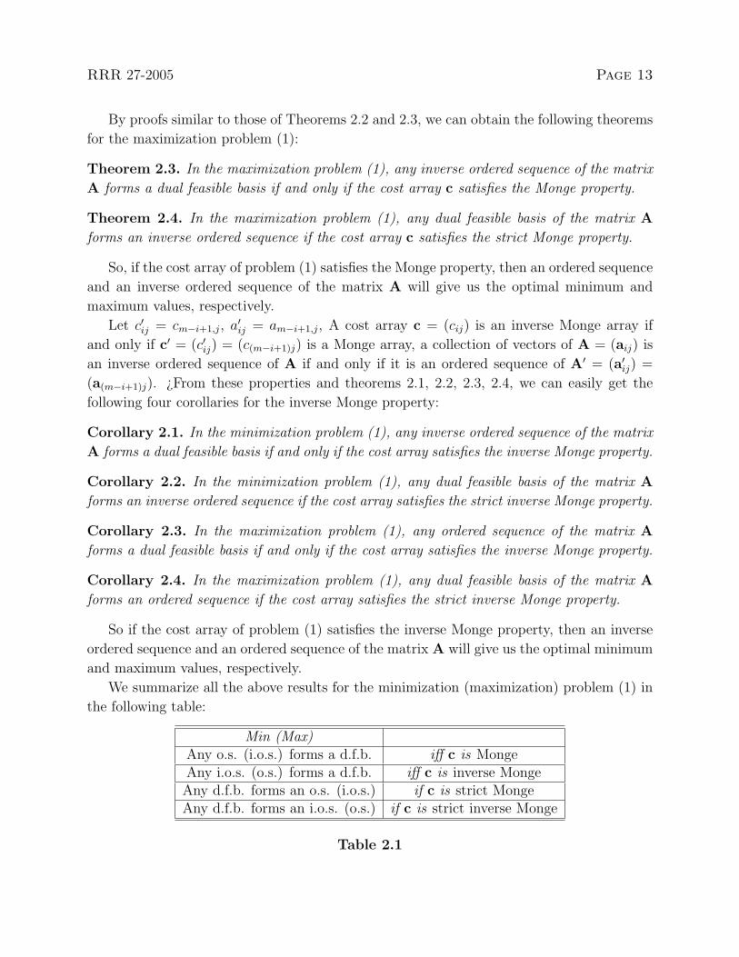
By proofs similar to those of Theorems 2.2 and 2.3, we can obtain the following theorems

for the maximization problem (1):

Theorem 2.3. In the maximization problem (1), any inverse ordered sequence of the matrix

A forms a dual feasible basis if and only if the cost array c satisfies the Monge property.

Theorem 2.4. In the maximization problem (1), any dual feasible basis of the matrix A

forms an inverse ordered sequence if the cost array c satisfies the strict Monge property.

So, if the cost array of problem (1) satisfies the Monge property, then an ordered sequence

and an inverse ordered sequence of the matrix A will give us the optimal minimum and

maximum values, respectively.

Let c′ij = cm−i+1,j, a′ij = am−i+1,j, A cost array c = (cij) is an inverse Monge array if

and only if c′ = (c′ij) = (c(m−i+1)j) is a Monge array, a collection of vectors of A = (aij) is

an inverse ordered sequence of A if and only if it is an ordered sequence of A′ = (a′ij) =

(a(m−i+1)j). ¿From these properties and theorems 2.1, 2.2, 2.3, 2.4, we can easily get the

following four corollaries for the inverse Monge property:

Corollary 2.1. In the minimization problem (1), any inverse ordered sequence of the matrix

A forms a dual feasible basis if and only if the cost array satisfies the inverse Monge property.

Corollary 2.2. In the minimization problem (1), any dual feasible basis of the matrix A

forms an inverse ordered sequence if the cost array satisfies the strict inverse Monge property.

Corollary 2.3. In the maximization problem (1), any ordered sequence of the matrix A

forms a dual feasible basis if and only if the cost array satisfies the inverse Monge property.

Corollary 2.4. In the maximization problem (1), any dual feasible basis of the matrix A

forms an ordered sequence if the cost array satisfies the strict inverse Monge property.

So if the cost array of problem (1) satisfies the inverse Monge property, then an inverse

ordered sequence and an ordered sequence of the matrix A will give us the optimal minimum

and maximum values, respectively.

We summarize all the above results for the minimization (maximization) problem (1) in

the following table:

Min (Max)Any o.s. (i.o.s.) forms a d.f.b. iff c is MongeAny i.o.s. (o.s.) forms a d.f.b. iff c is inverse MongeAny d.f.b. forms an o.s. (i.o.s.) if c is strict MongeAny d.f.b. forms an i.o.s. (o.s.) if c is strict inverse Monge

Table 2.1

RRR 27-2005

Here ”o.s.” means ordered sequence, ”i.o.s.” means inverse ordered sequence, and ”d.f.b.”

means dual feasible basis.

Next, we present the relationship between ordered sequences and the dual feasible bases

in the d-dimensional problem (2) (d > 2). So, the vectors x, c, b and the matrix A, we use

in the rest of this section, are those in (5).

To prove our results we recall three theorems, where the first two are well-known in linear

programming (see, Prekopa, 1996, Theorem 5 and 3).

Theorem 2.5. If problem (3) has a primal feasible solution and a finite optimum, then there

exists a primal feasible basis that is also dual feasible.

Theorem 2.6. If in problem (3) B is a primal feasible and nondegenerate basis (i.e., the

xB, determined by BxB = b, has all positive components) and B is optimal, i.e., (xB,xR)

is an optimal solution (xR = 0), then B is a dual feasible basis.

Bein et al (1995) extended the algorithm GREEDY2 to the algorithm GREEDYd and

proved the following theorem:.

Theorem 2.7. (Bein et al. 1995) Given a particular n1 × n2 × · · · × nd d-dimensional cost

array c, the algorithm GREEDYd solves the corresponding d-dimensional transportation

problem for any b if and only if c is Monge.

For d-dimensional minimization problem (2), we prove two theorems.

Theorem 2.8. In the minimization problem (2), any ordered sequence of the matrix A forms

a dual feasible basis if and only if the cost array c satisfies the Monge property.

Proof. For the proof of the ”if” direction, assume that c is Monge. For any given ordered

sequence, write positive numbers in the cells of it and what comes out on the r.h.s., let

it be the b. For this b, the algorithm GREEDYd produces the same ordered sequence, by

Theorem 2.7, this ordered sequence is a primal non-degenerate, optimal basis to the problem.

By Theorem 2.6, this ordered sequence is dual feasible.

For the proof of the ”only if” direction, assume that any ordered sequence of matrix

A forms a dual feasible basis. Then for any b the algorithm GREEDYd solves the prob-

lem optimally, because the algorithm GREEDYd produces an ordered sequence. Thus, by

Theorem 2.7, c is Monge.

To prove the next theorem, we need the dual of the minimization problem (2) which is

given as follows:

RRR 27-2005 Page 15

max∑d

k=1

∑nk

ik=1 ak(ik)wk(ik)

subject to

w1(i1) + · · ·+ wd(id) ≤ c(i1, . . . , id)

for all ik = 1, . . . , nk, k = 1, . . . , d.

(25)

Theorem 2.9. In the minimization problem (2), any dual feasible basis of the matrix A

forms an ordered sequence of A if the cost array c satisfies the strict Monge property.

Proof. Suppose that the cost array satisfies the strict Monge property, and B is a dual

feasible basis of matrix A. Assume that the vectors of B do not form an ordered sequence,

then there must exist vectors a(i1, . . . , id) and a(j1, . . . , jd) in B such that if sk = min{ik, jk},tk = max{ik, jk}, then (s1, . . . , sd) 6= (i1, . . . , id), (s1, . . . , sd) 6= (j1, . . . , jd). Let wk(ik),

ik = 1, . . . , nk, k = 1, . . . , d, be the components of dual vector corresponding to B. Then

c(i1, . . . , id) = w1(i1) + · · ·+ wd(id),

c(j1, . . . , jd) = w1(j1) + · · ·+ wd(jd),

c(s1, . . . , sd) ≥ w1(s1) + · · ·+ wd(sd),

c(t1, . . . , td) ≥ w1(t1) + · · ·+ wd(td).

Since

w1(i1) + · · ·+ wd(id) + w1(j1) + · · ·+ wd(jd)

= w1(s1) + · · ·+ wd(sd) + w1(t1) + · · ·+ wd(td), (26)

we have the relation

c(s1, . . . , sd) + c(t1, . . . , td) ≥ c(i1, . . . , id) + c(j1, . . . , jd).

It contradicts to the strict Monge property, so any dual feasible basis of the matrix A must

be an ordered sequence of A.

3 The Use of Covariance in The Two-Dimensional Case

In this section we consider the problem:

min(max)∑m

i=1

∑nj=1 cijxij

subject to ∑nj=1 xij = ai, i = 1, . . . ,m∑mi=1 xij = bj, j = 1, . . . , n∑mi=1

∑nj=1 yizjxij = c

xij ≥ 0, i = 1, . . . ,m, j = 1, . . . , n.

(27)

RRR 27-2005

The first m + n constraints in problem (27) prescribe that the univariate marginals are

{ai}, {bj}. Since the univariate marginals determine the univariate expectations, the last

constraint in (27) prescribes that the covariance between the two random variables is also

given. Assume that cij is a function of yi, zj: cij = g(yi, zj), i = 1, . . . ,m, j = 1, . . . , n.

Problem (27) can be written in the following matrix form:

max cTx

subject to

Ax = b

x ≥ 0,

(28)

where A = (aij), aij = ei + em+j + yizjem+n+1, i = 1, . . . ,m, j = 1, . . . , n, ei, em+j and

em+n+1 are unit vectors in Em+n+1 with ones in the i-th, (m + j)-th and (m + n + 1)-th

positions, respectively, b =

(bc

), and b, c and x are defined in (4).

Theorem 3.1. Consider the minimization problem (27), and assume that {yi} is strictly

increasing and {zj} is strictly decreasing, and the (1,2)-order and (2,1)-order divided dif-

ferences of g(yi, zj) are nonnegative. Then B1 = {ai1, i = 1, . . . ,m, amj, j = 2, . . . , n, a1n}forms a dual feasible basis of A.

Proof. First, let us show that B1 forms a basis of A. It is easy to see that the rank of A is

m + n, and there are m + n vectors in B1. To show the linear independence of the m + n

vectors in B1, consider the linear combination of the vectors of B1:

m∑i=1

λi1ai1 +n∑

j=2

λmjamj + λ1na1n

=m∑

i=1

λi1(ei + em+1 + yiz1em+n+1) +n∑

j=2

λmj(em + em+j + ymzjem+n+1)

+λ1n(e1 + em+n + y1znem+n+1)

= (λ11 + λ1n)e1 +m−1∑i=2

λi1ei + (n∑

j=1

λmj)em + (m∑

i=1

λi1)em+1 +n−1∑j=2

λmjem+j

+(λmn + λ1n)em+n + (m∑

i=1

λi1yiz1 +n∑

j=2

λmjymzj + λ1ny1zn)em+n+1.

If it equals 0, then, by the linear independence of the unit vectors, it follows that all λ’s

must be 0.

Secondly let us show that this basis is dual feasible. For any nonbasic vector aij, 1 ≤ i <

RRR 27-2005 Page 17

m, 1 < j ≤ n, we have the equations:

aij − ai1 + am1 − amj = (yi − ym)(zj − z1)em+n+1

aij − ai1 + a11 − a1n + amn − amj

= [(yi − ym)(zj − z1)− (y1 − ym)(zn − z1)]em+n+1.

¿From here we derive the expression of aij as the following linear combination of the basic

vectors:

aij =(y1 − ym)(z1 − zn)− (yi − ym)(z1 − zj)

(y1 − ym)(z1 − zn)(ai1 − am1 + amj)

− (yi − ym)(z1 − zj)

(y1 − ym)(z1 − zn)(a11 − a1n + amn − amj − ai1).

We have to prove that

(y1 − ym)(z1 − zn)− (yi − ym)(z1 − zj)

(y1 − ym)(z1 − zn)(ci1 − cm1 + cmj)

− (yi − ym)(z1 − zj)

(y1 − ym)(z1 − zn)(c11 − c1n + cmn − cmj − ci1)− cij ≤ 0,

or, what is the same,

(ci1 − cm1 + cmj − cij) ≤(yi − ym)(z1 − zj)

(y1 − ym)(z1 − zn)(c11 − cm1 + cmn − c1n). (29)

Since (yi − ym)(z1 − zj) < 0, the above inequality is equivalent to

ci1 − cm1 − cij + cmj

(yi − ym)(z1 − zj)≥ c11 − cm1 − c1n + cmn

(y1 − ym)(z1 − zn).

We have assumed that the (1,2)-order and (2,1)-order divided differences of g(yi, zj) are

nonnegative. The nonnegativity of the (1,2)-order divided difference implies

c11−cm1−c1n+cmn

(y1−ym)(z1−zn)− c11−cm1−c1j+cmj

(y1−ym)(z1−zj)

zn − zj

≥ 0.

Similarly, the nonnegativity of (2,1)-order divided difference gives

c11−cm1−c1j+cmj

(y1−ym)(z1−zj)− ci1−cm1−cij+cmj

(yi−ym)(z1−zj)

y1 − yi

≥ 0.

Since both zn − zj and y1 − yi are negative, the above two inequalities imply

ci1 − cm1 − cij + cmj

(yi − ym)(z1 − zj)≥ c11 − cm1 − c1j + cmj

(y1 − ym)(z1 − zj)≥ c11 − cm1 − c1n + cmn

(y1 − ym)(z1 − zn).

This completes the proof.

RRR 27-2005

The following corollaries follow at once from Theorem 3.1.

Corollary 3.1. Consider the minimization problem (27), and assume that {yi} is strictly

decreasing and {zj} is strictly increasing, and the (1,2)-order and (2,1)-order divided differ-

ences of g(yi, zj) are nonpositive. Then B1 forms a dual feasible basis of A.

Corollary 3.2. Consider the minimization problem (27), and assume that both {yi} and

{zj} are strictly increasing, the (1,2)-order divided difference of g(yi, zj) is nonnegative, and

the (2,1)-order divided difference of g(yi, zj) is nonpositive. Then B1 forms a dual feasible

basis of A.

Corollary 3.3. Consider the minimization problem (27), and assume that both {yi} and

{zj} are strictly decreasing, the (1,2)-order divided difference of g(yi, zj) is nonpositive, and

the (2,1)-order divided difference of g(yi, zj) is nonnegative. Then B1 forms a dual feasible

basis of A.

Corollary 3.4. Consider the maximization problem (27), and assume that {yi} is strictly

decreasing and {zj} is strictly increasing, and the (1,2)-order and (2,1)-order divided differ-

ences of g(yi, zj) are nonnegative. Then B1 forms a dual feasible basis of A.

Corollary 3.5. Consider the maximization problem (27), and assume that {yi} is strictly

increasing and {zj} is strictly decreasing, and the (1,2)-order and (2,1)-order divided differ-

ences of g(yi, zj) are nonpositive. Then B1 forms a dual feasible basis of A.

Corollary 3.6. Consider the maximization problem (27), and assume that both {yi} and

{zj} are strictly increasing, the (1,2)-order divided difference of g(yi, zj) is nonpositive, and

the (2,1)-order divided difference of g(yi, zj) is nonnegative. Then B1 forms a dual feasible

basis of A.

Corollary 3.7. Consider the maximization problem (27), and assume that both {yi} and

{zj} are strictly decreasing, the (1,2)-order divided difference of g(yi, zj) is nonnegative, and

the (2,1)-order divided difference of g(yi, zj) is nonpositive. Then B1 forms a dual feasible

basis of A.

If we use the reasoning in the proof of Theorem 3.1, we can obtain a variety of dual fea-

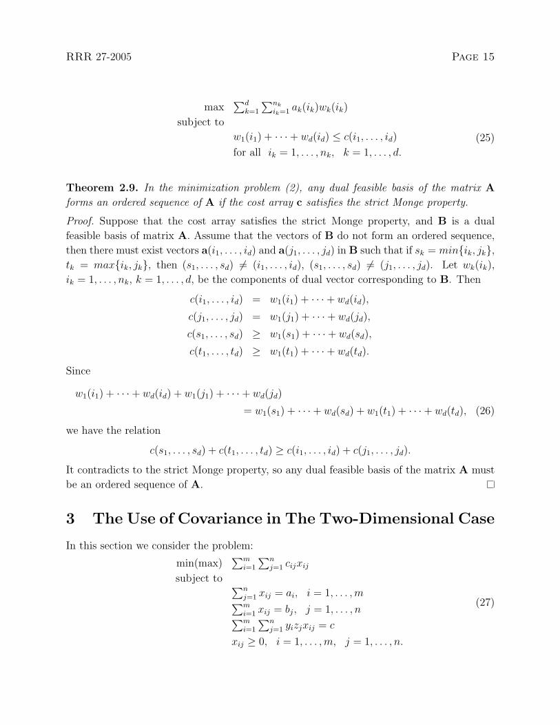
sible bases for problem (27) under different conditions. Let B2 = {ain, i = 1, . . . ,m, a1j, j =

1, . . . , n−1, am1}, B3 = {ai1, i = 1, . . . ,m, a1j, j = 2, . . . , n, amn}, B4 = {ain, i = 1, . . . ,m, amj, j =

1, . . . , n− 1, a11}, the cells corresponding to the vectors in B1, B2, B3 and B4 are designated

by boldface points in Figures 3.1, 3.2, 3.3 and 3.4, respectively.

RRR 27-2005 Page 19

s c a a a c s s s q q q s ss c a a a c c c c a a a c sqqq aaa aaa aaa aaa qqq aaa aaa aaa qqqs c a a a c c c c a a a c ss s q q q s s s c a a a c s

1 2 n-1 n 1 2 n-1 n1

2

m-1

m

1

2

m-1

m

Figure 3.1. (B1) Figure 3.2. (B2)

s s q q q s s s c a a a c ss c a a a c c c c a a a c sqqq aaa aaa aaa aaa qqq aaa aaa aaa qqqs c a a a c c c c a a a c ss c a a a c s s s q q q s s

1 2 n-1 n 1 2 n-1 n1

2

m-1

m

1

2

m-1

m

Figure 3.3. (B3) Figure 3.4. (B4)

We summarize all the results for the minimization (maximization) problem (27) in the

following table:

yi zj (1,2)-order d.d. (2,1)-order d.d. d.f.b. of min d.f.b. of max↗ ↘ ≥ 0 ≥ 0 B1 B2

↘ ↗ ≤ 0 ≤ 0 B1 B2

↗ ↗ ≥ 0 ≤ 0 B1 B2

↘ ↘ ≤ 0 ≥ 0 B1 B2

↗ ↘ ≤ 0 ≤ 0 B2 B1

↘ ↗ ≥ 0 ≥ 0 B2 B1

↗ ↗ ≤ 0 ≥ 0 B2 B1

↘ ↘ ≥ 0 ≤ 0 B2 B1

↗ ↘ ≤ 0 ≥ 0 B3 B4

↘ ↗ ≥ 0 ≤ 0 B3 B4

↗ ↗ ≤ 0 ≤ 0 B3 B4

↘ ↘ ≥ 0 ≥ 0 B3 B4

↗ ↘ ≥ 0 ≤ 0 B4 B3

↘ ↗ ≤ 0 ≥ 0 B4 B3

↗ ↗ ≥ 0 ≥ 0 B4 B3

↘ ↘ ≤ 0 ≤ 0 B4 B3

RRR 27-2005

Table 3.1

The sign ↗ means strictly increasing, while ↘ means strictly decreasing. ”d.d.” means

divided difference, and ”d.f.b.” means dual feasible basis.

4 The Three-Dimensional Case

In this section we look at the 3-dimensional transportation problem:

min(max)∑n1

i=1

∑n2

j=1

∑n3

k=1 cijkxijk

subject to ∑n2

j=1

∑n3

k=1 xijk = ai, i = 1, . . . , n1∑n1

i=1

∑n3

k=1 xijk = bj, j = 1, . . . , n2∑n1

i=1

∑n2

j=1 xijk = ck, k = 1, . . . , n3

xijk ≥ 0, i = 1, . . . , n1, j = 1, . . . , n2, k = 1, . . . , n3.

(30)

We can write problem (30) in matrix form if we let

x = (x111, . . . , x11n3 , . . . , x1n21, . . . , x1n2n3 , . . . ,

xn111, . . . , xn11n3 , . . . , xn1n21, . . . , xn1n2n3)T

c = (c111, . . . , c11n3 , . . . , c1n21, . . . , c1n2n3 , . . . ,

cn111, . . . , cn11n3 , . . . , cn1n21, . . . , cn1n2n3)T (31)

b = (a1, . . . , an1 , b1, . . . , bn2 , c1, . . . , cn3)T

A = (a111, . . . , a11n3 , . . . , a1n21, . . . , a1n2n3 , . . . ,

an111, . . . , an11n3 , . . . , an1n21, . . . , an1n2n3)T ,

where aijk = ei + en1+j + en1+n2+k and ei, en1+j and en1+n2+k are unit vectors in En1+n2+n3 ,

with ones in the ith, (n1+j)th and (n1+n2+k)th positions, respectively, for all i = 1, . . . , n1,

j = 1, . . . , n2, k = 1, . . . , n3. With these definitions problem (30) takes the form (3).

For this problem, we can get the following theorem:

Theorem 4.1. Consider the minimization problem (30), and assume that the cost array

satisfies the Monge property. Then each of the following six sequences of vectors forms a

dual feasible basis of the columns of the matrix A:

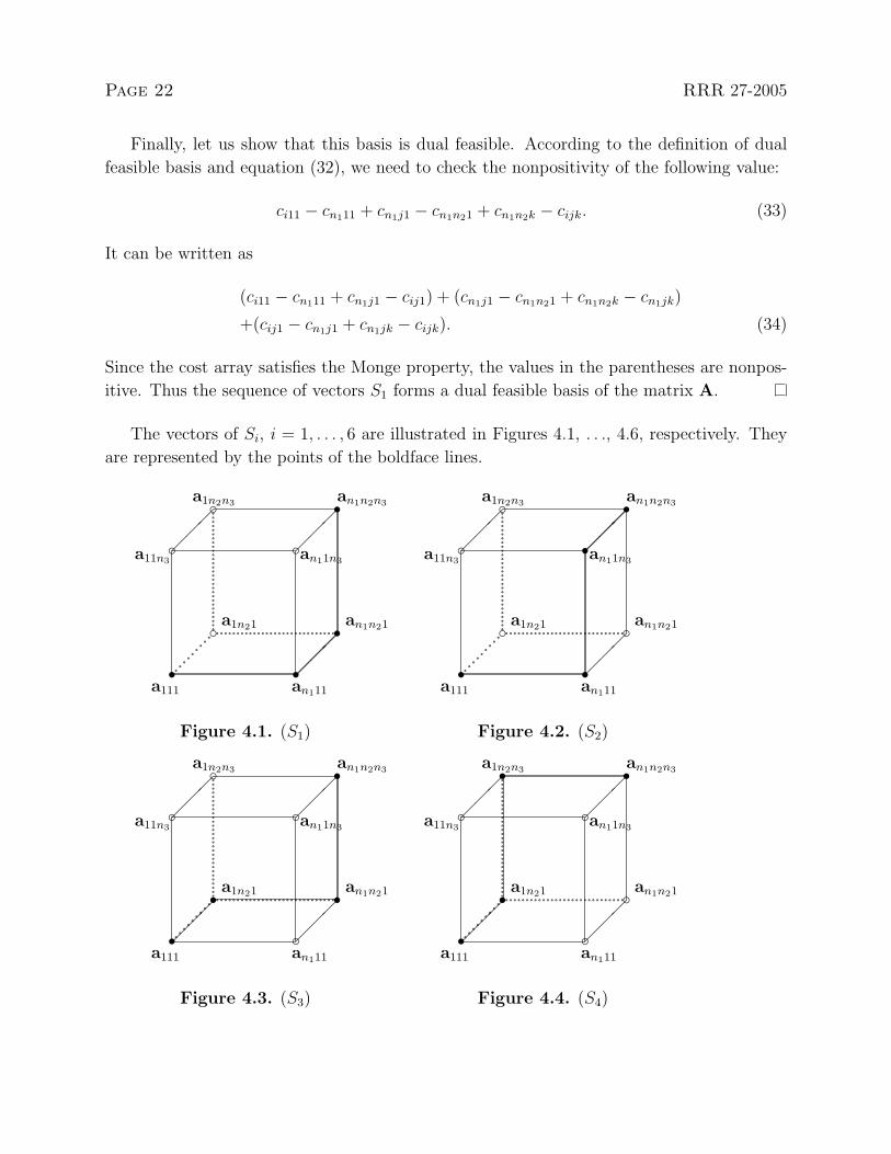
(S1) {ai11, i = 1, . . . , n1, an1j1, j = 2, . . . , n2, an1n2k, k = 2, . . . , n3},(S2) {ai11, i = 1, . . . , n1, an11k, k = 2, . . . , n3, an1jn3 , j = 2, . . . , n2},(S3) {a1j1, j = 1, . . . , n2, ain21, i = 2, . . . , n1, an1n2k, k = 2, . . . , n3},(S4) {a1j1, j = 1, . . . , n2, a1n2k, k = 2, . . . , n3, ain2n3 , i = 2, . . . , n1},(S5) {a11k, k = 1, . . . , n3, ai1n3 , i = 2, . . . , n1, an1jn3 , j = 2, . . . , n2},(S6) {a11k, k = 1, . . . , n3, a1jn3 , j = 2, . . . , n2, ain2n3 , i = 2, . . . , n1}.

RRR 27-2005 Page 21

Proof. Theorem 4.1 can easily be derived by the use of Theorem 2.8. In fact, each of (S1)-

(S6) is an ordered sequence. A direct proof, however, may be instructive and below we

present one.

First let us show that the vectors of S1 are independent. Consider the linear combination

of these vectors:

n1∑i=1

λi11ai11 +

n2∑j=2

λn1j1an1j1 +

n3∑k=2

λn1n2kan1n2k

=

n1∑i=1

λi11(ei + en1+1 + en1+n2+1) +

n2∑j=2

λn1j1(en1 + en1+j + en1+n2+1)

+

n3∑k=2

λn1n2k(en1 + en1+n2 + en1+n2+k)

=

n1−1∑i=1

λi11ei + (

n2∑j=1

λn1j1 +

n3∑k=2

λn1n2k)en1 + (

n1∑i=1

λi11)en1+1

+

n2−1∑j=2

λn1j1en1+j + (

n3∑k=1

λn1n2k)en1+n2

+(

n1∑i=1

λi11 +

n2−1∑j=2

λn1j1)en1+n2+1 +

n3∑k=2

λn1n2ken1+n2+k.

We can see that if it equals 0, then all λ’s must be 0.

Next we show that any vector aijk of the matrix A can be expressed as a linear combi-

nation of these vectors, 1 ≤ i ≤ n1, 1 ≤ j ≤ n2, 1 ≤ k ≤ n3. In fact,

aij1 − an1j1 + an1jk

= ei + en1+j + en1+n2+1 − (en1 + en1+j + en1+n2+1)

+en1 + en1+j + en1+n2+k

= ei + en1+j + en1+n2+k

= aijk,

aij1 = ai11 − an111 + an1j1,

an1jk = an1j1 − an1n21 + an1n2k,

so,

aijk = ai11 − an111 + an1j1 − an1n21 + an1n2k, (32)

where ai11, an111, an1j1, an1n21, an1n2k ∈ S1. Thus S1 forms a basis of matrix A.

RRR 27-2005

Finally, let us show that this basis is dual feasible. According to the definition of dual

feasible basis and equation (32), we need to check the nonpositivity of the following value:

ci11 − cn111 + cn1j1 − cn1n21 + cn1n2k − cijk. (33)

It can be written as

(ci11 − cn111 + cn1j1 − cij1) + (cn1j1 − cn1n21 + cn1n2k − cn1jk)

+(cij1 − cn1j1 + cn1jk − cijk). (34)

Since the cost array satisfies the Monge property, the values in the parentheses are nonpos-

itive. Thus the sequence of vectors S1 forms a dual feasible basis of the matrix A.

The vectors of Si, i = 1, . . . , 6 are illustrated in Figures 4.1, . . ., 4.6, respectively. They

are represented by the points of the boldface lines.

s s s sc s c c

c c c sc s c s

` ` ` ` ` ` ` ``

` ` ` ` ` ` ` ```

```

````

` ` ` ` ` ` ` ` ` ` ` ` ` ` ` ` ` ` ` ` ` ` ` ` ` ` ` ` ` ` ` ` ` ` ` ` ` ` ` ` ` ` ` ` ` ` ` ` ` ` ` ` ` ` ` ` ` `�

��

��

�

��

�

��

�

��

�

��

�

��

�

��

�

a111 an111 a111 an111

a1n21 an1n21 a1n21 an1n21


a1n2n3 an1n2n3 a1n2n3 an1n2n3

Figure 4.1. (S1) Figure 4.2. (S2)

s c s cs s s c

c c c cc s s s

` ` ` ` ` ` ` ``

` ` ` ` ` ` ` ```

```

````

` ` ` ` ` ` ` ` ` ` ` ` ` ` ` ` ` ` ` ` ` ` ` ` ` ` ` ` ` ` ` ` ` ` ` ` ` ` ` ` ` ` ` ` ` ` ` ` ` ` ` ` ` ` ` ` ` `�

��

��

�

��

�

��

�

��

�

��

�

��

�

��

�

a111 an111 a111 an111





RRR 27-2005 Page 23

s c s cc c c c

s s s cc s s s

` ` ` ` ` ` ` ``

` ` ` ` ` ` ` ```

```

````

` ` ` ` ` ` ` ` ` ` ` ` ` ` ` ` ` ` ` ` ` ` ` ` ` ` ` ` ` ` ` ` ` ` ` ` ` ` ` ` ` ` ` ` ` ` ` ` ` ` ` ` ` ` ` ` ` `�

��

��

�

��

�

��

�

��

�

��

�

��

�

��

�

a111 an111 a111 an111





Theorem 4.2. Consider the maximization problem (30). If the cost array satisfies the

Monge property, then each of the following sequences of vectors forms a dual feasible basis

of the matrix A:

(S ′1) {ai11, i = 1, . . . , n1, a1j1, j = 2, . . . , n2, a11k, k = 2, . . . , n3},

(S ′2) {ain2n3 , i = 1, . . . , n1, an1jn3 , j = 1, . . . , n2 − 1,

an1n2k, k = 1, . . . , n3 − 1}.

Proof. We prove the assertion for S ′1. The proof for the other one can be carried out similarly.

First we show that these vectors are independent. Consider the linear combination of the

vectors of S ′1:

n1∑i=1

λi11ai11 +

n2∑j=2

λ1j1a1j1 +

n3∑k=2

λ11ka11k

=

n1∑i=1

λi11(ei + en1+1 + en1+n2+1) +

n2∑j=2

λ1j1(e1 + en1+j + en1+n2+1)

+

n3∑k=2

λ11k(e1 + en1+1 + en1+n2+k)

= (

n2∑j=1

λ1j1 +

n3∑k=2

λ11k)e1 +

n1∑i=2

λi11ei + (

n1∑i=1

λi11 +

n3∑k=2

λ11k)en1+1

+

n2∑j=2

λ1j1en1+j + (

n1∑i=1

λi11 +

n2∑j=2

λ1j1)en1+n2+1 +

n3∑k=2

λ11ken1+n2+k.

We can easily see that if it is 0, then all λ’s are zero.

RRR 27-2005

Secondly we show that any vector aijk of the matrix A can be expressed as a linear

combination of the vectors in S ′1. In fact, we have the relations:

aij1 − ai11 + ai1k

= ei + en1+j + en1+n2+1 − (ei + en1+1 + en1+n2+1)

+ei + en1+1 + en1+n2+k

= ei + en1+j + en1+n2+k

= aijk,

aij1 = ai11 − a111 + a1j1,

ai1k = ai11 − a111 + a11k.

Then

aijk = ai11 − a111 + a11k − a111 + a1j1, (35)

where ai11, a111, a11k, a1j1 ∈ S ′1. So S ′

1 forms a basis of the matrix A.

Thirdly we show that this basis is dual feasible. According to the definition of the dual

feasibility of a basis for the maximization problem and equation (35), we need to prove the

nonnegativity of the following value:

ci11 − c111 + c11k − c111 + c1j1 − cijk. (36)

The value (36) can be written as

(ci11 − c111 + c11k − ci1k) + (ci11 − cij1 + c1j1 − c111)

+(ci1k − ci11 + cij1 − cijk). (37)

Since the cost array satisfies the Monge property, the values in the three parentheses are

nonnegative. Thus the sequence of vectors S ′1 forms a dual feasible basis of the matrix A in

the maximization problem (30).

The vectors of S ′1 and S ′

2 are illustrated in Figures 4.7 and 4.8, respectively. They are

represented by the points of the boldface lines.

RRR 27-2005 Page 25

s s c cs c c s

s c c sc c s s

` ` ` ` ` ` ` ``

` ` ` ` ` ` ` ```

```

````

` ` ` ` ` ` ` ` ` ` ` ` ` ` ` ` ` ` ` ` ` ` ` ` ` ` ` ` ` ` ` ` ` ` ` ` ` ` ` ` ` ` ` ` ` ` ` ` ` ` ` ` ` ` ` ` ` `�

��

��

�

��

�

��

�

��

�

��

�

��

�

��

�

a111 an111 a111 an111




Figure 4.7. (S ′1) Figure 4.8. (S ′

2)

5 The Use of Covariances in The Three-Dimensional

Case

In this section we supplement the covariance constraints to the constraints of problem (30).

The new problem is the following:

min(max)∑n1

i=1

∑n2

j=1

∑n3

k=1 cijkxijk

subject to ∑n2

j=1

∑n3

k=1 xijk = ai, i = 1, . . . , n1∑n1

i=1

∑n3

k=1 xijk = bj, j = 1, . . . , n2∑n1

i=1

∑n2

j=1 xijk = ck, k = 1, . . . , n3∑n1

i=1

∑n2

j=1

∑n3

k=1 risjxijk = d1∑n1

i=1

∑n2

j=1

∑n3

k=1 sjtkxijk = d2∑n1

i=1

∑n2

j=1

∑n3

k=1 ritkxijk = d3

xijk ≥ 0, i = 1, . . . , n1, j = 1, . . . , n2, k = 1, . . . , n3.

(38)

Assume that there is a map between ri, sj, tk and cijk, i.e., cijk = g(ri, sj, tk), for i =

1, . . . , n1, j = 1, . . . , n2, k = 1, . . . , n3. Problem (38), can be written in the compact form

RRR 27-2005

(28), where

A = (aijk) =

Arsstrt

b =

(bd

)rs = (r1s1, . . . , r1s1, . . . , r1sn2 , . . . , r1sn2 , . . . ,

rn1s1, . . . , rn1s1, . . . , rn1sn2 , . . . , rn1sn2)

st = (s1t1, . . . , s1t1, . . . , s1tn3 , . . . , s1tn3 , . . . ,

sn2t1, . . . , sn2t1, . . . , sn2tn3 , . . . , sn2tn3) (39)

rt = (r1t1, . . . , r1t1, . . . , r1tn3 , . . . , r1tn3 , . . . ,

rn1t1, . . . , rn1t1, . . . , rn1tn3 , . . . , rn1tn3)

d = (d1, d2, d3)T ,

and A, b, c, x are the same as in (31).

Let S1 be the collection of those vectors aijk which have the same subscripts as those in

S1 in Theorem 4.1. We prove

Theorem 5.1. Consider the minimization problem (38). If ri, sj and tk are strictly in-

creasing, all (1, 2, 0)-order, (1, 0, 2)-order, (0, 1, 2)-order divided differences of g(ri, sj, tk) are

nonnegative, and all (2, 1, 0)-order, (2, 0, 1)-order and (0, 2, 1)-order and (1, 1, 1)-order di-

vided differences of g(ri, sj, tk) are nonpositive, then S1 ∪ {an11n3 , a1n21, a11n3} forms a dual

feasible basis of the matrix A.

Proof. First let us show that vectors of the sequence S1 and the vectors an11n3 , a1n21 and

a11n3 form a basis of A. By Theorem 4.1 S1 forms a basis of A, and the basis of A has at

most three more vectors than the basis of A. So, we only need to prove that these vectors are

linearly independent. It is, however true, because we have the equation (for n1 +n2 +n3 +3-

dimensional vectors)

∑n1

i=1 λi11ai11 +∑n2

j=2 λn1j1an1j1 +∑n3

k=2 λn1n2kan1n2k

+λn11n3an11n3 + λ1n21a1n21 + λ11n3a11n3

RRR 27-2005 Page 27

=

λ111 + λ1n21 + λ11n3

λ211...

λ(n1−1)11

λn111 + · · ·+ λn1n21 + · · ·+ λn1n2n3 + λn11n3

λ111 + · · ·+ λn111 + λn11n3 + λ11n3

λn121...

λn1(n2−1)1

λn1n21 + · · ·+ λn1n2n3 + λ1n21

λ111 + · · ·+ λn111 + · · ·+ λn1n21 + λ1n21

λn1n22...

λn1n2(n3−1)

λn1n2n3 + λn11n3 + λ11n3

r1s1λ111 + · · ·+ rn1s1λn111 + · · ·+ rn1sn2λn1n21 + · · ·+ rn1sn2λn1n2n3

+rn1s1λn11n3 + r1sn2λ1n21 + r1s1λ11n3

s1t1λ111 + · · ·+ s1t1λn111 + · · ·+ sn2t1λn1n21 + · · ·+ sn2tn3λn1n2n3

+s1tn3λn11n3 + sn2t1λ1n21 + s1tn3λ11n3

r1t1λ111 + · · ·+ rn1t1λn111 + · · ·+ rn1t1λn1n21 + · · ·+ rn1tn3λn1n2n3

+rn1tn3λn11n3 + r1t1λ1n21 + r1tn3λ11n3

and if it equals 0, then all λ’s must be 0.

Secondly, let us show that this basis is dual feasible. Assume that all {ri}, {sj} and {tk}sequences are strictly decreasing. The proof for the case where all ri, sj and tk are strictly

increasing can be carried out the same way. For any nonbasic vector aijk, 1 ≤ i ≤ n1,

1 ≤ j ≤ n2, 1 ≤ k ≤ n3, we have the following four equations:

aijk − ai11 + an111 − an1j1 + an1n21 − an1n2k

=

0

(ri − rn1)(sj − s1)(sj − sn2)(tk − t1)(ri − rn1)(tk − t1)

, (40)

aijk − ai11 + an111 − an1n2k + an1n2n3 − an11n3 + an111 − an1j1

=

0

(ri − rn1)(sj − s1)(sj − sn2)(tk − t1)− (s1 − sn2)(tn3 − t1)

(ri − rn1)(tk − t1)

, (41)

RRR 27-2005

aijk − an1j1 + an1n21 − an1n2k + an11n3 − a11n3 + a111 − ai11

=

0

(ri − rn1)(sj − s1)(sj − sn2)(tk − t1)

(ri − rn1)(tk − t1)− (r1 − rn1)(tn3 − t1)

, (42)

aijk − ai11 + a111 − a1n21 + an1n21 − an1j1 + an1n21 − an1n2k

=

0

(ri − rn1)(sj − s1)− (r1 − rn1)(sn2 − s1)(sj − sn2)(tk − t1)(ri − rn1)(tk − t1)

, (43)

where 0 is a zero vector in Rn1+n2+n3 . For simplicity, let

A1 = (ri − rn1)(sj − s1),

A2 = (sj − sn2)(tk − t1),

A3 = (ri − rn1)(tk − t1),

B1 = (r1 − rn1)(sn2 − s1),

B2 = (s1 − sn2)(tn3 − t1),

B3 = (r1 − rn1)(tn3 − t1),

a13 =

0A1

0A3

, a12 =

0A1

A2

0

, a23 =

00A2

A3

.

¿From (40) and (41) we obtain

A2 −B2

A2

(aijk − ai11 + an111 − an1j1 + an1n21 − an1n2k − a13)

= aijk − ai11 + an111 − an1n2k + an1n2n3 − an11n3 + an111 − an1j1 − a13.

Thus,

aijk = (ai11 − an111 + an1j1 − an1n21 + an1n2k + a13)

−A2

B2

(an1n2n3 − an11n3 + an111 − an1n21). (44)

Equations (40) and (42) imply


−A3

B3

(an11n3 − a11n3 + a111 − an111). (45)

RRR 27-2005 Page 29

Similarly, equations (40) and (43) imply


−A1

B1

(a111 − a1n21 + an1n21 − an111). (46)

Finally, from the definition of a13, a12, a23 and (38), we derive the relation:

a13 + a12 + a23 = 2(aijk − ai11 + an111 − an1j1 + an1n21 − an1n2k).

Summing up (41), (42) and (43), we find that

aijk = ai11 − an111 + an1j1 − an1n21 + an1n2k

−A2

B2

(an1n2n3 − an11n3 + an111 − an1n21)

−A3

B3

(an11n3 − a11n3 + a111 − an111) (47)

−A1

B1

(a111 − a1n21 + an1n21 − an111).

To prove the dual feasibility, we need to prove that

ci11 − cn111 + cn1j1 − cn1n21 + cn1n2k

−A2

B2

(cn1n2n3 − cn11n3 + cn111 − cn1n21)

−A3

B3

(cn11n3 − c11n3 + c111 − cn111)

−A1

B1

(c111 − c1n21 + cn1n21 − cn111)− cijk ≤ 0,

or, what is the same,

(ci11 − cn111 + cn1j1 − cij1)

+(cij1 − cn1j1 + cn1jk − cijk)

+(cn1j1 − cn1n21 + cn1n2k − cn1jk)

≤ A2

B2

(cn1n2n3 − cn11n3 + cn111 − cn1n21) (48)

+A3

B3

(cn11n3 − c11n3 + c111 − cn111)

+A1

B1

(c111 − c1n21 + cn1n21 − cn111)

RRR 27-2005

If we fix one of the i, j, k subscripts in cijk, then, in view of Corollary 2.6, (29) will hold

for the remaining two subscripts. Thus we can obtain the following inequalities:

ci11 − cn111 + cn1j1 − cij1 ≤A1

B1

(c111 − c1n21 + cn1n21 − cn111), (49)

cn1j1 − cn1n21 + cn1n2k − cn1jk ≤A2

B2

(cn1n2n3 − cn11n3 + cn111 − cn1n21), (50)

cij1 − cn1j1 + cn1jk − cijk ≤A3

B3

(cn1jn3 − c1jn3 + c1j1 − cn1j1). (51)

Also, from the nonpositivity of the (1,1,1)-order divided difference of g(ri, sj, tk), we obtain

c111−cn111−c11n3+cn11n3

(r1−rn1 )(t1−tn3 )− c1j1−cn1j1−c1jn3

+cn1jn3

(r1−rn1 )(t1−tn3 )

(s1 − sj)≤ 0,

where s1 − sj < 0, r1 − rn1 < 0, t1 − tn3 < 0. This implies

c1j1 − cn1j1 − c1jn3 + cn1jn3 ≤ c111 − cn111 − c11n3 + cn11n3 .

By (51) and the inequality A3

B3> 0, we have

cij1 − cn1j1 + cn1jk − cijk ≤A3

B3

(c111 − cn111 − c11n3 + cn11n3). (52)

Summing up (49), (50) and (52), we can obtain (48). Thus the basis is dual feasible.

By the similar proof, we can obtain the following theorem

Theorem 5.2. Under the same conditions with Theorem 5.1 except that (1, 1, 1)-order di-

vided differences of g(ri, sj, tk) are nonnegative, then S1∪{an11n3 , a1n21, a1n2n3} forms a dual

feasible basis of the matrix A.

RRR 27-2005 Page 31

Define S2, . . ., S6, S ′1, S ′

2 the same way as we have defined S1. Let

S11 = S1 ∪ {an11n3 , a1n21, a11n3},S12 = S1 ∪ {an11n3 , a1n21, a1n2n3},S21 = S2 ∪ {a11n3 , an1n21, a1n21},S22 = S2 ∪ {a11n3 , an1n21, a1n2n3},S31 = S3 ∪ {an111, a1n2n3 , a11n3},S32 = S3 ∪ {an111, a1n2n3 , an11n3},S41 = S4 ∪ {a11n3 , an1n21, an111},S42 = S4 ∪ {a11n3 , an1n21, an11n3},S51 = S5 ∪ {an111, a1n2n3 , a1n21},S52 = S5 ∪ {an111, a1n2n3 , an1n21},S61 = S6 ∪ {a1n21, an11n3 , an111},S62 = S6 ∪ {a1n21, an11n3 , an1n21},S ′

11 = S ′1 ∪ {an1n21, an11n3 , a1n2n3},

S ′12 = S ′

1 ∪ {an1n21, an11n3 , an1n2n3},S ′

13 = S ′1 ∪ {an1n21, an1n2n3 , a1n2n3},

S ′14 = S ′

1 ∪ {an1n2n3 , an11n3 , a1n2n3},S ′

21 = S ′2 ∪ {an111, a1n21, a11n3},

S ′22 = S ′

2 ∪ {an111, a1n21, a111},S ′

23 = S ′2 ∪ {an111, a111, a11n3},

S ′24 = S ′

2 ∪ {a111, a1n21, a11n3}.

Then we can derive results for the three-dimensional problem (38), we present them in Tables

5.1-5.8. In the following tables, ↗ means strictly increasing, ↘ means strictly decreasing,

(i, j, k) means (i, j, k)-order divided difference, 0 ≤ i, j, k ≤ 2, ’d.f.b. of min’ and ’d.f.b. of

max’ mean ’dual feasible basis of the minimization problem (38)’ and ’dual feasible basis of

the maximization problem (38)’, respectively.

RRR 27-2005

ri ↗ ↗ ↗ ↘ ↗ ↘ ↘ ↘sj ↗ ↗ ↘ ↗ ↘ ↗ ↘ ↘tk ↗ ↘ ↗ ↗ ↘ ↘ ↗ ↘

(1, 2, 0) ≥ 0 ≥ 0 ≥ 0 ≤ 0 ≥ 0 ≤ 0 ≤ 0 ≤ 0(2, 1, 0) ≤ 0 ≤ 0 ≥ 0 ≤ 0 ≥ 0 ≤ 0 ≥ 0 ≥ 0(1, 0, 2) ≥ 0 ≥ 0 ≥ 0 ≤ 0 ≥ 0 ≤ 0 ≤ 0 ≤ 0(2, 0, 1) ≤ 0 ≥ 0 ≤ 0 ≤ 0 ≥ 0 ≥ 0 ≤ 0 ≥ 0(0, 1, 2) ≥ 0 ≥ 0 ≤ 0 ≥ 0 ≤ 0 ≥ 0 ≤ 0 ≤ 0(0, 2, 1) ≤ 0 ≥ 0 ≤ 0 ≤ 0 ≥ 0 ≥ 0 ≤ 0 ≥ 0(1, 1, 1) ≤ 0 ≥ 0

(≥ 0) (≤ 0)

d.f.b. S11

of min (S12)

d.f.b. S62

of max (S61)

Table 5.1

ri ↗ ↗ ↗ ↘ ↗ ↘ ↘ ↘sj ↗ ↗ ↘ ↗ ↘ ↗ ↘ ↘tk ↗ ↘ ↗ ↗ ↘ ↘ ↗ ↘

(1, 2, 0) ≤ 0 ≤ 0 ≤ 0 ≥ 0 ≤ 0 ≥ 0 ≥ 0 ≥ 0(2, 1, 0) ≥ 0 ≥ 0 ≤ 0 ≥ 0 ≤ 0 ≥ 0 ≤ 0 ≤ 0(1, 0, 2) ≤ 0 ≤ 0 ≤ 0 ≥ 0 ≤ 0 ≥ 0 ≥ 0 ≥ 0(2, 0, 1) ≥ 0 ≤ 0 ≥ 0 ≥ 0 ≤ 0 ≤ 0 ≥ 0 ≤ 0(0, 1, 2) ≤ 0 ≤ 0 ≥ 0 ≤ 0 ≥ 0 ≤ 0 ≥ 0 ≥ 0(0, 2, 1) ≥ 0 ≤ 0 ≥ 0 ≥ 0 ≤ 0 ≤ 0 ≥ 0 ≤ 0(1, 1, 1) ≤ 0 ≥ 0

(≥ 0) (≤ 0)

d.f.b. S61

of min (S62)

d.f.b. S12

of max (S11)

Table 5.2

RRR 27-2005 Page 33

ri ↗ ↗ ↗ ↘ ↗ ↘ ↘ ↘sj ↗ ↗ ↘ ↗ ↘ ↗ ↘ ↘tk ↗ ↘ ↗ ↗ ↘ ↘ ↗ ↘

(1, 2, 0) ≥ 0 ≥ 0 ≥ 0 ≤ 0 ≥ 0 ≤ 0 ≤ 0 ≤ 0(2, 1, 0) ≤ 0 ≤ 0 ≥ 0 ≤ 0 ≥ 0 ≤ 0 ≥ 0 ≥ 0(1, 0, 2) ≥ 0 ≥ 0 ≥ 0 ≤ 0 ≥ 0 ≤ 0 ≤ 0 ≤ 0(2, 0, 1) ≤ 0 ≥ 0 ≤ 0 ≤ 0 ≥ 0 ≥ 0 ≤ 0 ≥ 0(0, 1, 2) ≤ 0 ≤ 0 ≥ 0 ≤ 0 ≥ 0 ≤ 0 ≥ 0 ≥ 0(0, 2, 1) ≥ 0 ≤ 0 ≥ 0 ≥ 0 ≤ 0 ≤ 0 ≥ 0 ≤ 0(1, 1, 1) ≤ 0 ≥ 0

(≥ 0) (≤ 0)

d.f.b. S21

of min (S22)

d.f.b. S42

of max (S41)

Table 5.3

ri ↗ ↗ ↗ ↘ ↗ ↘ ↘ ↘sj ↗ ↗ ↘ ↗ ↘ ↗ ↘ ↘tk ↗ ↘ ↗ ↗ ↘ ↘ ↗ ↘

(1, 2, 0) ≤ 0 ≤ 0 ≤ 0 ≥ 0 ≤ 0 ≥ 0 ≥ 0 ≥ 0(2, 1, 0) ≥ 0 ≥ 0 ≤ 0 ≥ 0 ≤ 0 ≥ 0 ≤ 0 ≤ 0(1, 0, 2) ≤ 0 ≤ 0 ≤ 0 ≥ 0 ≤ 0 ≥ 0 ≥ 0 ≥ 0(2, 0, 1) ≥ 0 ≤ 0 ≥ 0 ≥ 0 ≤ 0 ≤ 0 ≥ 0 ≤ 0(0, 1, 2) ≥ 0 ≥ 0 ≤ 0 ≥ 0 ≤ 0 ≥ 0 ≤ 0 ≤ 0(0, 2, 1) ≤ 0 ≥ 0 ≤ 0 ≤ 0 ≥ 0 ≥ 0 ≤ 0 ≥ 0(1, 1, 1) ≤ 0 ≥ 0

(≥ 0) (≤ 0)

d.f.b. S41

of min (S42)

d.f.b. S22

of max (S21)

Table 5.4

RRR 27-2005

ri ↗ ↗ ↗ ↘ ↗ ↘ ↘ ↘sj ↗ ↗ ↘ ↗ ↘ ↗ ↘ ↘tk ↗ ↘ ↗ ↗ ↘ ↘ ↗ ↘

(1, 2, 0) ≤ 0 ≤ 0 ≤ 0 ≥ 0 ≤ 0 ≥ 0 ≥ 0 ≥ 0(2, 1, 0) ≥ 0 ≥ 0 ≤ 0 ≥ 0 ≤ 0 ≥ 0 ≤ 0 ≤ 0(1, 0, 2) ≥ 0 ≥ 0 ≥ 0 ≤ 0 ≥ 0 ≤ 0 ≤ 0 ≤ 0(2, 0, 1) ≤ 0 ≥ 0 ≤ 0 ≤ 0 ≥ 0 ≥ 0 ≤ 0 ≥ 0(0, 1, 2) ≥ 0 ≥ 0 ≤ 0 ≥ 0 ≤ 0 ≥ 0 ≤ 0 ≤ 0(0, 2, 1) ≤ 0 ≥ 0 ≤ 0 ≤ 0 ≥ 0 ≥ 0 ≤ 0 ≥ 0(1, 1, 1) ≤ 0 ≥ 0

(≥ 0) (≤ 0)

d.f.b. S31

of min (S32)

d.f.b. S52

of max (S51)

Table 5.5

ri ↗ ↗ ↗ ↘ ↗ ↘ ↘ ↘sj ↗ ↗ ↘ ↗ ↘ ↗ ↘ ↘tk ↗ ↘ ↗ ↗ ↘ ↘ ↗ ↘

(1, 2, 0) ≥ 0 ≥ 0 ≥ 0 ≤ 0 ≥ 0 ≤ 0 ≤ 0 ≤ 0(2, 1, 0) ≤ 0 ≤ 0 ≥ 0 ≤ 0 ≥ 0 ≤ 0 ≥ 0 ≥ 0(1, 0, 2) ≤ 0 ≤ 0 ≤ 0 ≥ 0 ≤ 0 ≥ 0 ≥ 0 ≥ 0(2, 0, 1) ≥ 0 ≤ 0 ≥ 0 ≥ 0 ≤ 0 ≤ 0 ≥ 0 ≤ 0(0, 1, 2) ≤ 0 ≤ 0 ≥ 0 ≤ 0 ≥ 0 ≤ 0 ≥ 0 ≥ 0(0, 2, 1) ≥ 0 ≤ 0 ≥ 0 ≥ 0 ≤ 0 ≤ 0 ≥ 0 ≤ 0(1, 1, 1) ≤ 0 ≥ 0

(≥ 0) (≤ 0)

d.f.b. S51

of min (S52)

d.f.b. S32

of max (S31)

Table 5.6

RRR 27-2005 Page 35

ri ↗ ↗ ↗ ↘ ↗ ↘ ↘ ↘sj ↗ ↗ ↘ ↗ ↘ ↗ ↘ ↘tk ↗ ↘ ↗ ↗ ↘ ↘ ↗ ↘

(1, 2, 0) ≤ 0 ≤ 0 ≤ 0 ≥ 0 ≤ 0 ≥ 0 ≥ 0 ≥ 0(2, 1, 0) ≤ 0 ≤ 0 ≥ 0 ≤ 0 ≥ 0 ≤ 0 ≥ 0 ≥ 0(1, 0, 2) ≤ 0 ≤ 0 ≤ 0 ≥ 0 ≤ 0 ≥ 0 ≥ 0 ≥ 0(2, 0, 1) ≤ 0 ≥ 0 ≤ 0 ≤ 0 ≥ 0 ≥ 0 ≤ 0 ≥ 0(0, 1, 2) ≤ 0 ≤ 0 ≥ 0 ≤ 0 ≥ 0 ≤ 0 ≥ 0 ≥ 0(0, 2, 1) ≤ 0 ≥ 0 ≤ 0 ≤ 0 ≥ 0 ≥ 0 ≤ 0 ≥ 0(1, 1, 1) ≥ 0 ≤ 0

(≤ 0) (≥ 0)

d.f.b. S ′11

of min (S ′12, S ′

13, or S ′14)

d.f.b. S ′22, S ′

23, or S ′24

of max (S ′21)

Table 5.7

ri ↗ ↗ ↗ ↘ ↗ ↘ ↘ ↘sj ↗ ↗ ↘ ↗ ↘ ↗ ↘ ↘tk ↗ ↘ ↗ ↗ ↘ ↘ ↗ ↘

(1, 2, 0) ≥ 0 ≥ 0 ≥ 0 ≤ 0 ≥ 0 ≤ 0 ≤ 0 ≤ 0(2, 1, 0) ≥ 0 ≥ 0 ≤ 0 ≥ 0 ≤ 0 ≥ 0 ≤ 0 ≤ 0(1, 0, 2) ≥ 0 ≥ 0 ≥ 0 ≤ 0 ≥ 0 ≤ 0 ≥ 0 ≤ 0(2, 0, 1) ≥ 0 ≤ 0 ≥ 0 ≥ 0 ≤ 0 ≤ 0 ≥ 0 ≤ 0(0, 1, 2) ≥ 0 ≥ 0 ≤ 0 ≥ 0 ≤ 0 ≥ 0 ≤ 0 ≤ 0(0, 2, 1) ≥ 0 ≤ 0 ≥ 0 ≥ 0 ≤ 0 ≤ 0 ≥ 0 ≤ 0(1, 1, 1) ≤ 0 ≥ 0

(≥ 0) (≤ 0)

d.f.b. S ′22, S ′

23, or S ′24

of min (S ′21)

d.f.b. S ′11

of max (S ′12, S ′

13, or S ′14)

Table 5.8

RRR 27-2005

6 Applications and Illustrative Examples

Monge and inverse Monge arrays came up in many practical applications. A collection of

them is presented in Burkard et al. (1996). In this section we present three more applications

which, at the same time, illustrate the ways that we can make use the results of the present

paper.

6.1 Bounding Unknown Entries in Partially Known Arrays

As we have mentioned in the Introduction, any dual feasible bases in an LP may serve

for bounding and approximation of unknown components of the coefficient vector of the

objective function. If B1 (B2) is a dual feasible basis in a minimization (maximization)

problem such that cB1 (cB2) is known, then we have the bound for any unknown ck:

yTak ≤ ck (53)

(yTak ≥ ck),

where y is any solution of the equation yTB1 = cTB1

(yTB2 = cTB2

). The best theoretical

bound is the largest (smallest) of all these bounds.

In Sections 2 and 4 we have presented dual feasible bases for LP’s with Monge arrays in

the objective function. We have done the same in Sections 3 and 5 for some higher order

convex objective function coefficient arrays. Thus, we have created methods for bounding

the entries of the above-mentioned arrays, if they are only partially known. If both the lower

and upper bounds can be given for ck and the bounds are close, then they may be used for

the approximation of that value.

The dual feasibility of a basis, however, does not depend on the right hand side values in

the equality constraints. Therefore, the bounds presented in Sections 2-5 may not be close

enough to the unknown value. There are two possibilities to improve on them.

The first one is to carry out steps according to the rules of the dual method. Any time

when a dual step is carried out, first we decide on the vector that leaves the basis B and the

right hand side values in the constraints, to do that. As regards the entering vector, we can

find one as long as there is an ak such that ck is known and ak can enter the basis according

to the rules of the dual method. Whenever no further ak can be included into the basis,

either because primal feasible basis has been found or the corresponding ck is unknown, then

we take the best bound so far as our final (lower or upper) bound.

The second one is the reduction of the size of the problem. This can be done only in

connection with the problems discussed in Sections 2 and 4, unless the available information

allows for applying it to problems in Sections 3 and 5.

In the problems of Sections 2 and 4 the right hand side values, i.e., the univariate marginal

distributions are fully known, by assumption, so are the univariate marginal conditional

RRR 27-2005 Page 37

distributions, given that the univariate random variables are restricted to some subsets of

the support sets. The new problem, written up with the conditional probabilities on the right

hand side, becomes smaller and the bounds for the unknown entries of the Monge array in

the objective function may be better. This method can be applied for problems described

in Sections 3 and 5 only if the conditional covariances are also known.

Any distribution array is a Monge array and the entries of a distribution array are values

of a probability distribution function. Hence, the methodology of Sections 2, 4 provides us

with a methodology for bounding and approximation of unknown values of a multivariate

discrete p.d.f.. The results of Sections 3 and 5 improve on the bounds. In those cases

the distribution functions must have the special property: nonnegativity of some divided

differences.

Example 6.1 In the problem (1), the known cij and ai,bj values are given in the

following table:

a4 = 14 c41 = 22 c42 = 20 c43 = 20 c44 = 16 c45 = 12 c46 = 13a3 = 39 c31 = 17 c32 c33 c34 c35 c36 = 12a2 = 22 c21 = 17 c22 c23 c24 c25 c26 = 20a1 = 18 c11 = 8 c12 = 10 c13 = 13 c14 = 11 c15 = 14 c16 = 23

b1 = 10 b2 = 11 b3 = 13 b4 = 20 b5 = 24 b6 = 15

Table 6.1

To find the lower bounds for the unknown values of cij, we choose

L1 = {a11, a12, a13, a14, a15, a16, a26, a36, a46}

as the initial dual feasible basis. Carrying out the dual method, no more dual feasible basis

can be obtained. Since the solution of the equation yT1 L1 = cT

L1is yT

1 = (23, 20, 12, 13,−15,−13,−10,−12,−9, 0),

the lower bounds for the unknown cij obtained from the dual feasible basis L1 are as follows:

c22 ≥ 7, c23 ≥ 10, c24 ≥ 8, c25 ≥ 11,

c32 ≥ −1, c33 ≥ 2, c34 ≥ 0, c35 ≥ 3.

Again we can choose

L2 = {a11, a21, a31, a41, a42, a43, a44, a45, a46}

as the initial dual feasible basis. Carrying out the dual method, no more dual feasible basis

can be obtained. Since the solution of the equation yT2 L2 = cT

L2is yT

2 = (−1, 8, 8, 13, 9, 7, 7, 3,−1, 0),

the lower bounds for the unknown cij obtained from the dual feasible basis L2 are as follows:

c22 ≥ 15, c23 ≥ 15, c24 ≥ 11, c25 ≥ 7,

c32 ≥ 15, c33 ≥ 15, c34 ≥ 11, c35 ≥ 7.

RRR 27-2005

So the final lower bounds for the unknown cij are as follows:

c22 ≥ 15, c23 ≥ 15, c24 ≥ 11, c25 ≥ 11,

c32 ≥ 15, c33 ≥ 15, c34 ≥ 11, c35 ≥ 7.

To find the upper bounds for the unknown values of cij, similarly we choose

U1 = {a16, a15, a14, a13, a12, a11, a21, a31, a41}

or

U2 = {a16, a26, a36, a46, a45, a44, a43, a42, a41}.

as the initial dual feasible basis. The final upper bounds for the unknown cij are as

follows:

c22 ≤ 19, c23 ≤ 22, c24 ≤ 20, c25 ≤ 19,

c32 ≤ 19, c33 ≤ 19, c34 ≤ 15, c35 ≤ 11.

Example 6.2 In example 6.1, if one more constraint is given with the form of the last

constraint in problem (27), where

c = 1076, y1 = 1, y2 = 2, y3 = 3, y4 = 4,

z1 = 16, z2 = 9, z3 = 4, z4 = 3, z5 = 2, z6 = 1,

then we can get a problem with the form of problem (27). It is easy to see that {yi} is

strictly increasing and {zj} is strictly decreasing. Assume that cij = g(yi, zj), then both

the (1,2)-order and (2,1)-order divided differences are nonpositive. According to the results

obtained in Section 3,

B2 = {a11, a12, a13, a14, a15, a16, a26, a36, a46, a41},

B1 = {a11, a21, a31, a41, a42, a43, a44, a45, a46, a16}

are the dual feasible bases of the minimization and maximization problems respectively.

¿From these two bases, the lower and upper bounds for the unknown cij can be obtained as

follows:

11.3 ≤ c22 ≤ 22.5, 11.6 ≤ c23 ≤ 27.8,

9.07 ≤ c24 ≤ 24.9, 11.5 ≤ c25 ≤ 21.9,

7.53 ≤ c32 ≤ 18.7, 5.2 ≤ c33 ≤ 21.4,

2.13 ≤ c34 ≤ 17.9, 4.07 ≤ c35 ≤ 14.5.

RRR 27-2005 Page 39

6.2 Bounding Expectations

Let X, Y be two independent random vectors with the same discrete support set. Suppose

that the probability distribution of X is fully known but the distribution of Y is only partially

known. We know all univariate marginal distributions of its components and, if d = 2 or 3,

all covariances of the pairs. Then we can give lower and upper bounds for

P (X ≤ Y ). (54)

Each lower or upper bound is based on a dual feasible basis. Any dual feasible basis that

we presented in Sections 2-5 provides us with a bound. If the basis is both primal and

dual feasible, then the bound is sharp, no better bound can be given based on the available

information. If we use our dual feasible bases as initial bases and carry out the lexicographic

dual method, then the last basis is both primal and dual feasible, and the optimum value of

the problem is the sharp bound.

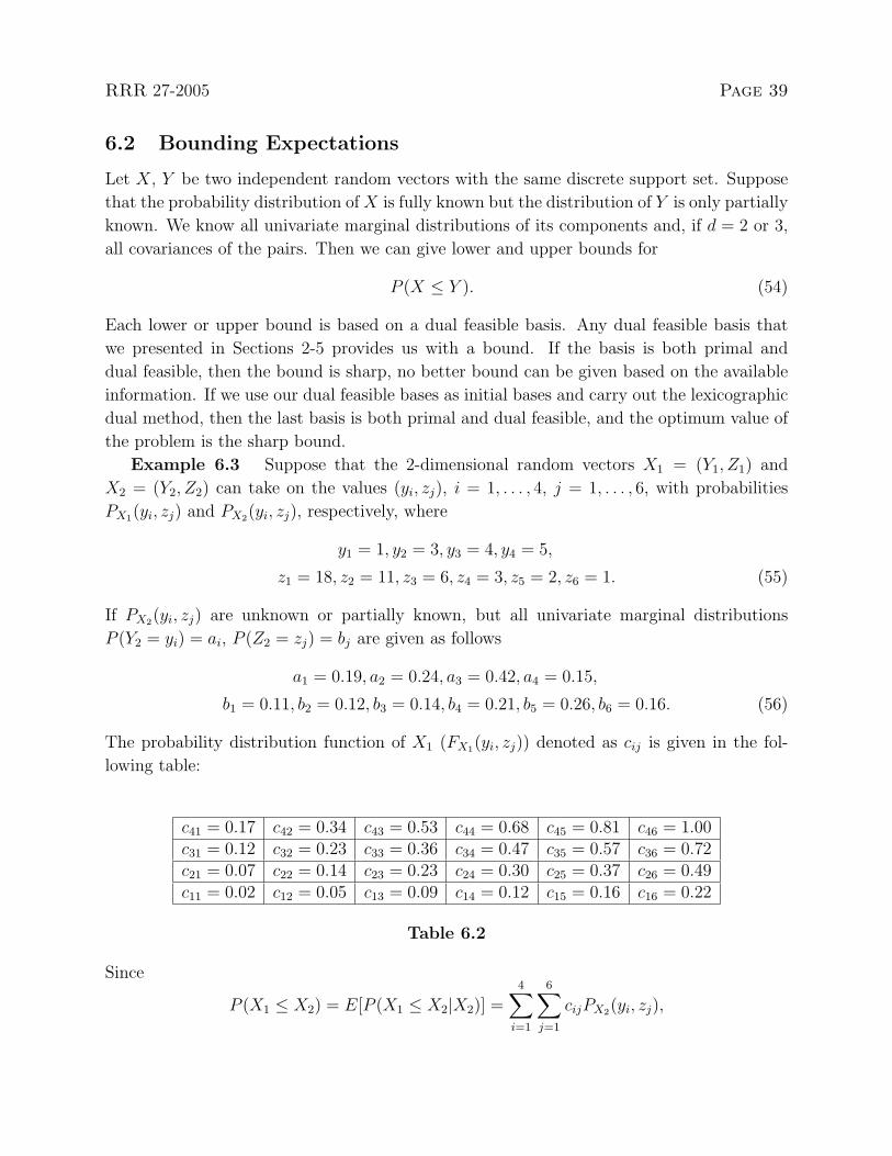
Example 6.3 Suppose that the 2-dimensional random vectors X1 = (Y1, Z1) and

X2 = (Y2, Z2) can take on the values (yi, zj), i = 1, . . . , 4, j = 1, . . . , 6, with probabilities

PX1(yi, zj) and PX2(yi, zj), respectively, where

y1 = 1, y2 = 3, y3 = 4, y4 = 5,

z1 = 18, z2 = 11, z3 = 6, z4 = 3, z5 = 2, z6 = 1. (55)

If PX2(yi, zj) are unknown or partially known, but all univariate marginal distributions

P (Y2 = yi) = ai, P (Z2 = zj) = bj are given as follows

a1 = 0.19, a2 = 0.24, a3 = 0.42, a4 = 0.15,

b1 = 0.11, b2 = 0.12, b3 = 0.14, b4 = 0.21, b5 = 0.26, b6 = 0.16. (56)

The probability distribution function of X1 (FX1(yi, zj)) denoted as cij is given in the fol-

lowing table:

c41 = 0.17 c42 = 0.34 c43 = 0.53 c44 = 0.68 c45 = 0.81 c46 = 1.00c31 = 0.12 c32 = 0.23 c33 = 0.36 c34 = 0.47 c35 = 0.57 c36 = 0.72c21 = 0.07 c22 = 0.14 c23 = 0.23 c24 = 0.30 c25 = 0.37 c26 = 0.49c11 = 0.02 c12 = 0.05 c13 = 0.09 c14 = 0.12 c15 = 0.16 c16 = 0.22

Table 6.2

Since

P (X1 ≤ X2) = E[P (X1 ≤ X2|X2)] =4∑

i=1

6∑j=1

cijPX2(yi, zj),

RRR 27-2005

the lower and upper bounds for P (X1 ≤ X2) can be obtained by solving the minimization

and maximization problems (1) with the ai, bj and cij values provided in (56) and Table 6.2.

Taking into account that the cij values satisfy inverse Monge property, we choose

L1 = {a11, a12, a13, a14, a15, a16, a21, a31, a41}

as the initial dual feasible basis for the minimization problem. Carrying out the lexicographic

dual method, we obtain a sequence of dual feasible bases. The last one is also primal feasible,

whose subscripts are {33, 34, 24, 25, 15, 16,

32, 42, 41}. Thus the optimum value 0.3232 is the lower bound for P (X1 ≤ X2). Similarly,

solving the maximization problem, we obtain a sequence of dual feasible bases The last

one is also primal feasible, whose subscripts are {11, 12, 22, 23, 24, 34, 35, 36, 46}. Thus the

optimum value 0.4381 is the upper bound for P (X1 ≤ X2). Therefore, the sharp bounds for

P (X1 ≤ X2) are as follows:

0.3232 ≤ P (X1 ≤ X2) ≤ 0.4381.

Example 6.4 In Example 6.3, suppose that the covariance of Y2 and Z2 is −5.003.

Since

E[Y2] =∑4

i=1 yiai = 3.34,

E[Z2] =∑6

j=1 zjbj = 5.45,

E[Y2Z2] =4∑

i=1

6∑j=1

yizjPX2(yi, zj)

= Cov(Y2, Z2) + E[Y2]E[Z2] (57)

= −5.003 + (3.34)(5.45) = 13.2.

Furthermore, the bounding problem can be formulated as the minimization and maximiza-

tion problems (27) with one more constraint described in (57).

Assume that cij = g(yi, zj), then the (1,2)-order divided difference of g(yi, zj) is nonneg-

ative and the (2,1)-order divided difference of g(yi, zj) is nonpositive. Then

B4 = {a16, a26, a36, a46, a41, a42, a43, a44, a45, a11}

and

B3 = {a11, a21, a31, a41, a12, a13, a14, a15, a16, a46}

are the initial dual feasible bases for the minimization and maximization problems, respec-

tively. Carrying out the lexicographic dual method, we obtain a sequence of dual feasi-

ble bases for the minimization and maximization problems, respectively. The subscripts

RRR 27-2005 Page 41

of the last ones, which are also primal feasible, are {22, 26, 25, 35, 12, 33, 43, 44, 34, 11} and

{11, 21, 24, 36, 12, 13, 23,

34, 35, 46} for the minimization and maximization problems, respectively. Thus the optimum

values are also the bounds for P (X1 ≤ X2) as follows:

0.4084 ≤ P (X1 ≤ X2) ≤ 0.4337.

These bounds improve the ones in Example 6.3.

6.3 The Wasserstein Distance of Two Probability Distributions

The Wasserstein distance between the probability distributions µ and ν, defined in Rn, is

the value:

W (µ, ν) = infπ∈Π

√∫ ∫1

2d(x, y)2dπ(x, y), (58)

where Π is the set of all probability distributions in Rn × Rn with marginals µ and ν,

respectively, i.e., if π ∈ Π, then π(◦×Rn)) = µ, π(Rn×◦)) = ν and d(x, y) is the Euclidean

distance between x and y.

Let n = 1 and µ, ν be the discrete distributions with supports {y1, . . . , ym}, {z1, . . . , zn}and corresponding probabilities {ai}, {bj}, respectively. Then

W 2(µ, ν) = min∑m

i=1

∑nj=1

12(yi − zj)

2xij

subject to∑nj=1 xij = ai, i = 1, . . . ,m∑mi=1 xij = bj, j = 1, . . . , n

xij ≥ 0, i = 1, . . . ,m, j = 1, . . . , n.

(59)

Assume that both {yi} and {zj} are increasing sequences. It is easy to see that the array

cij =1

2(yi − zj)

2, i = 1, . . . ,m, j = 1, . . . , n

has the Monge property (its (1, 1)-order divided difference is constant, equal to −1).

By Hoffman’s result, the greedy algorithm, described in Section 1.3, solves optimally

problem (59).

By Theorem 2.1 the objective function value, corresponding to any ordered sequence of

the transportation min problem, is a lower bound on W 2(µ, ν). That ordered sequence which

is also primal feasible, provides us with the exact value of W 2(µ, ν).

RRR 27-2005

7 Conclusions

We have presented results in connection with multivariate probability distributions with

given marginals and given covariances of the pairs of random variables involved. We have

also formulated optimization problems, where the coefficient array of the objective function

is supposed to have the Monge, or inverse Monge property, or is a special higher order convex

function.

We have reformulated basic results, obtained in connection with Monge arrays, in terms

of dual feasible bases in the two-, three- and multidimensional transportation problem. We

have also obtained general results in connection with the structures of dual feasible bases in

the two- and three-dimensional cases, where the constraints of the transportation problems

are supplemented by covariance constraints.

Our results allow for creating lower and upper bounds for unknown entries in partially

known Monge and inverse Monge arrays. We have also shown how the results can be used

to obtain lower and upper bounds for the expectation of a function of a discrete random

vector, where the function is a Monge or inverse Monge array and the univariate marginal

distributions are known. In the two- and three-dimensional cases we have obtained improved

bounds under the condition that the covariances of the pairs of the random variables are

also known. In this case the coefficient array of the objective function is supposed to have

some special higher order convexity property.

Illustrative numerical results have been presented and we mentioned some among the

many possible applications of our results.

References

[1] A. Aggarwal and J. K. Park, Parallel Searching in Multidimensional Monotone Arrays,Research Report RC 14826, IBM T. J. Watson Research Center, Yorktown Heights,NY, 1989. Submitted to J. Algorithms. Portions of this paper appear in Proceedingsof the 29th Annual IEEE Symposium on Foundations of Computer Science (1988), pp.497-512.

[2] A. Aggarwal and J. K. Park, Sequential Searching in Multidimensional Monotone Ar-rays, Research Report RC 15128, IBM T. J. Watson Research Center, Yorktown Heights,NY, 1989. Submitted to J. Algorithms. Portions of this paper appear in Proceedingsof the 29th Annual IEEE Symposium on Foundations of Computer Science (1988), pp.497-512.

[3] w. w. Bein and P. K. Pathak, A Characterization of The Monge Property, TechnicalReport CS90-11, Department of Computer Science, University of New Mexico, Albu-querque, New Mexico, 1990.

RRR 27-2005 Page 43

[4] W. W. Bein, P. Brucker, J. K. Park and P. K. Pathak, A Monge Property for thed-dimensional Transportation Problem, Discrete Appl. Math., 58 (1995), pp. 97-109.

[5] R. E. Burkard, B. Klinz and R. Rudolf, Perspectives of Monge Properties in Optimiza-tion, Discrete Applied Mathematics 60 (1996), pp. 95-161.

[6] R. E. Burkard, Monge Properties, discrete convexity and applications, Tech. Report 328,Graz University of Technology, 2004.

[7] K. Cechlarova and P. Szabo, On the Monge Property of Matrices, Discrete Math., 81(1990), pp. 123-128.

[8] G. Hadley, Linear Programming, Addison Wesley, Reading, MA, 1963.

[9] A. J. Hoffman, On Simple Linear Programming Problems, V. Klee,ed, Proc. Sympos.Pure Math., Convexity VII (1963), pp. 317-327.

[10] C. Jordan, Calculus of Finite Differences, Chelsea Publishing Company, New York,1947.

[11] I. Olkin and S. T. Rachev, Distribution with Given Marginals Subject to Certain Con-straints, Tech. Report 270, Department of Statistics, Stanford University, Stanford, CA,1990.

[12] T. Popoviciu, Les Fonctions Convexes, Actualites Scientifiques et Industrielles, 992,Hermann, Paris, 1994.

[13] A. Prekopa, Stochastic Programming. Budapest, Kluwer, 1995.

[14] A. Prekopa, A Brief Introduction to Linear Programming, Math. Sci., 21 (1996), pp.85-111.

[15] A. Prekopa, Bounds on Probabilities and Expectations Using Multivariate Moments ofDiscrete Distributions Studia Sci. Math. Hungar., 34 (1998), pp. 349-378.

[16] S. T. Rachev, Probability Metrics and the Stability of Stochastic Models, Wiley, Chich-ester, New York, 1991.

[17] R. Rudolf, Recognition of d-dimensional Monge Arrays, Discrete Appl. Math., 52 (1994),pp. 71-82.

Monge Property and Bounding Multivariate Probability Distribution Functions with Given Marginals and...

Documents

Transcript of Monge Property and Bounding Multivariate Probability Distribution Functions with Given Marginals and...