Longitudinal design considerations to optimize power to detect variances and covariances among rates...
23
Psychological Methods Longitudinal Design Considerations to Optimize Power to Detect Variances and Covariances Among Rates of Change: Simulation Results Based on Actual Longitudinal Studies Philippe Rast and Scott M. Hofer Online First Publication, November 11, 2013. doi: 10.1037/a0034524 CITATION Rast, P., & Hofer, S. M. (2013, November 11). Longitudinal Design Considerations to Optimize Power to Detect Variances and Covariances Among Rates of Change: Simulation Results Based on Actual Longitudinal Studies. Psychological Methods. Advance online publication. doi: 10.1037/a0034524
Transcript of Longitudinal design considerations to optimize power to detect variances and covariances among rates...

Psychological Methods
Longitudinal Design Considerations to Optimize Power toDetect Variances and Covariances Among Rates ofChange: Simulation Results Based on Actual LongitudinalStudiesPhilippe Rast and Scott M. HoferOnline First Publication, November 11, 2013. doi: 10.1037/a0034524
CITATIONRast, P., & Hofer, S. M. (2013, November 11). Longitudinal Design Considerations toOptimize Power to Detect Variances and Covariances Among Rates of Change: SimulationResults Based on Actual Longitudinal Studies. Psychological Methods. Advance onlinepublication. doi: 10.1037/a0034524
Longitudinal Design Considerations to Optimize Power to Detect Variancesand Covariances Among Rates of Change: Simulation Results Based on
Actual Longitudinal Studies
Philippe Rast and Scott M. HoferUniversity of Victoria
We investigated the power to detect variances and covariances in rates of change in the context ofexisting longitudinal studies using linear bivariate growth curve models. Power was estimated by meansof Monte Carlo simulations. Our findings show that typical longitudinal study designs have substantialpower to detect both variances and covariances among rates of change in a variety of cognitive, physicalfunctioning, and mental health outcomes. We performed simulations to investigate the interplay amongnumber and spacing of occasions, total duration of the study, effect size, and error variance on power andrequired sample size. The relation between growth rate reliability (GRR) and effect size to the samplesize required to detect power greater than or equal to .80 was nonlinear, with rapidly decreasing samplesizes needed as GRR increases. The results presented here stand in contrast to previous simulation resultsand recommendations (Hertzog, Lindenberger, Ghisletta, & von Oertzen, 2006; Hertzog, von Oertzen,Ghisletta, & Lindenberger, 2008; von Oertzen, Ghisletta, & Lindenberger, 2010), which are limited dueto confounds between study length and number of waves, error variance with growth curve reliability,and parameter values that are largely out of bounds of actual study values. Power to detect change isgenerally low in the early phases (i.e., first years) of longitudinal studies but can substantially increaseif the design is optimized. We recommend additional assessments, including embedded intensivemeasurement designs, to improve power in the early phases of long-term longitudinal studies.
Keywords: statistical power, growth rate reliability, individual differences in change, longitudinal design,study optimization
Supplemental materials: http://dx.doi.org/10.1037/a0034524.supp
Most questions in the study of developmental and aging-relatedprocesses pertain to “change” in systems of variables and acrossdifferent time scales. Typical longitudinal studies focus on change
processes over months and years, whereas “intensive measure-ment” studies examine change and variation across much shorterperiods (e.g., Walls, Barta, Stawski, Collyer, & Hofer, 2011).Although the design of particular longitudinal studies relies onboth theoretical rationale and previous empirical results, there isgeneral agreement that longitudinal data are necessary in order toapproach questions regarding developmental and aging-relatedchange within individuals (e.g., Bauer, 2011; Hofer & Sliwinski,2006; Schaie & Hofer, 2001). Optimally, the design of the longi-tudinal study will provide estimates of reliable within-personchange and variation in the processes of interest.
In order to model individual differences in change in longitudi-nal settings, multilevel models are a frequent choice (Laird &Ware, 1982; Raudenbush & Bryk, 2002) because they allow theflexible specification of both fixed (i.e., average) and randomeffects (i.e., individual departures from the average effect). Thedegree to which individuals change differently over time is in thevariance of a time-based slope, which can be expanded to covari-ances in the multivariate case involving two or more processesover time (e.g., MacCallum, Kim, Malarkey, & Kiecolt-Glaser,1997; McArdle, 1988). The covariance among the random slopesprovides information whether, and how strongly, these processesare associated. For example, Hofer et al. (2009) report associationsamong individual differences in level, rate of change, andoccasion-specific variation across subscales of the DevelopmentalBehavior Checklist (DBC) in a sample (N � 506) aged 5–19 years
Philippe Rast and Scott M. Hofer, Department of Psychology, Universityof Victoria, Victoria, British Columbia, Canada.
Preparation of this article in part was supported by the Swiss NationalScience Foundation (Grant SNSF-131511) and the Integrative Analysis ofLongitudinal Studies of Aging (IALSA) research network (NIHAG026453, P01AG043362). This research has been enabled by the use ofcomputing resources provided by WestGrid and Compute/Calcul Canada.We thank Andrea Piccinin and Catharine Sparks for their assistance instatistical analysis of IALSA-related studies and Belaid Moa for the im-plementation of OpenMx on the Nestor cluster. We gratefully thank thefollowing for contributing their study data for purposes of this article:Dorly Deeg (Longitudinal Aging Study Amsterdam), Roger Dixon (Vic-toria Longitudinal Study), Stewart Einfeld (Australian Child to AdultDevelopment Study), Boo Johansson (Origins of Variance in the Old-Old:Octogenarian Twins), Bonnie Leadbeater (Victoria Healthy Youth Sur-vey), K. Warner Schaie (Seattle Longitudinal Study), Bruce Tonge (Aus-tralian Child to Adult Development Study), Sherry Willis (Seattle Longi-tudinal Study), and Elizabeth Zelinski (Long Beach Longitudinal Study).
Correspondence concerning this article should be addressed to PhilippeRast or Scott M. Hofer, Department of Psychology, University of Victoria,P.O. Box 3050 STN CSC, Victoria, BC V8W 3P5, Canada. E-mail:[email protected] or [email protected]
Thi
sdo
cum
ent
isco
pyri
ghte
dby
the
Am
eric
anPs
ycho
logi
cal
Ass
ocia
tion
oron
eof
itsal
lied
publ
ishe
rs.
Thi
sar
ticle
isin
tend
edso
lely
for
the
pers
onal
use
ofth
ein
divi
dual
user
and
isno
tto
bedi
ssem
inat
edbr
oadl
y.
Psychological Methods © 2013 American Psychological Association2013, Vol. 18, No. 4, 000 1082-989X/13/$12.00 DOI: 10.1037/a0034524
1

and at four occasions over an 11-year period. Correlations amongthe five DBC subscales ranged from .43 to .66 for level, .43 to .88for linear rates of change, and .31 to .61 for occasion-specificresiduals, with the highest correlations observed consistently be-tween Disruptive (D), Self-Absorbed (SA), and CommunicationDisturbance behaviors. In addition to the mean trends (Einfeld etal., 2006), the pattern of these interdependencies among dimen-sions of emotional and behavioral disturbance provides insight intothe developmental dynamics of psychopathology from childhoodthrough young adulthood.
The power to detect the variance and covariance of variablesover time is a fundamental issue in associative and predictivemodels of change. Although a number of authors have dealt withquestions of sample size planning and power in the context oflongitudinal studies (e.g., Hedeker, Gibbons, & Waternaux, 1999;Kelley & Rausch, 2011; Maxwell, 1998; Maxwell, Kelley, &Rausch, 2008; B. O. Muthén & Curran, 1997), relatively few havespecifically addressed the power to estimate individual differencesin change and associations among rates of change (but see Hert-zog, Lindenberger, Ghisletta, & von Oertzen, 2006; Hertzog, vonOertzen, Ghisletta, & Lindenberger, 2008; von Oertzen, Ghisletta,& Lindenberger, 2010).
The estimation of power to detect change and correlated changein longitudinal designs requires consideration of a number ofcritical parameters, each having potential differential effects on theresults. Briefly, following early work by Willett (1989), we dif-ferentiate between parameters that are not typically under controlof the researcher, such as the variability of change over time (i.e.,individual differences in slope �S
2), the correlation betweenchanges over time (i.e., covariance of slopes �SySx
), the measure-ment error variance (�ε
2), and features of the study design that aremodifiable such as the sample size (N), the spacing and number ofmeasurement assessments, and the total span or duration of thestudy. These parameters and design features are directly linked tothe reliability to detect individual growth curves (cf. Willett,1989), which is partly given by the reliability of the measures butcan be considerably altered by the study design.
Hence, the purpose of this work is to cast light on the interplayamong different factors that contribute to the detection of individ-ual differences in and among rates of change. It is important toknow how our decisions regarding longitudinal designs impactpower to detect certain effects. In this regard it is of special interestto identify features of the study design that are modifiable and thatcan be used to optimize power and with it sample size require-ments. An important tool to identify the relevant parameters andtheir interplay is the reliability of the growth rate as proposed byWillett (1989).
Growth Rate Reliability
The reliability of the growth rate is central to the analysis ofchange. In the context of longitudinal multilevel models, the firststep usually involves the estimation of an intraclass correlationcoefficient (ICC), an index of the ratio of between-subject variance(�class
2 ) to total variance. This is done by estimating an uncondi-tional means model whereby the variance due to differences be-tween persons in a repeated-measures setting is expressed as aproportion of the total variance �class
2 /(�class2 � �ε
2) (cf. Raudenbush& Bryk, 2002). If the number of measurement occasions is the
same for all participants in a study, the ICC can be expanded toobtain a measure of reliability. Thereby, the residual variance (�ε
2)is divided by the number of measurement occasions to obtain theICC2 estimate (Bliese, 2000). The ICC2 indicates how much of thebetween-person variation in observed scores is due to true scorevariation (see also Kuljanin, Braun, & DeShon, 2011).
To obtain an estimate of the reliability of the growth rate, Willett(1989) presented an index that bears some similarity to the reli-ability estimate ICC2. Willett’s index, however, takes into accountthe design of the study by dividing the residual variance �ε
2 by the sumof squared deviations of time points (�) about the mean at measure-
ment occasions (w) in W waves, SST � �w�1W ��w � ���2. Hence,
Willett defines growth rate reliability (GRR) as
GRR ��S
2
�S2 � � ��
2
SST�. (1)
The GRR estimate provides critical information about the capa-bility to distinguish individual differences in the slope parametersbut should not be mistaken for an index of reliability of themeasurement instrument, as “it confounds the unrelated influencesof group heterogeneity in growth-rate and measurement precision”(Willett, 1989, p. 595). For instance, in a situation with no indi-vidual differences in slope, GRR will be 0 even if the reliability ofthe measurement is high. At the same time, this feature is desirablefor the purpose of understanding and identifying critical designparameters because it takes into account the increasing difficulty todetect slope variances as they approach 0. Hence, GRR is wellsuited for the identification of critical design parameters thatinfluence the ability to detect individual differences in growthrates. As Willett showed, the reliability of individual growth isdependent on several factors, including the magnitude of interin-dividual heterogeneity in growth (�S
2); the size of the measurementerror variance (�ε
2); and total sum of squared deviations of timepoints (SST), which is dependent on the number of waves (W); thespacing or interval between these waves; and the total duration ofa study. Besides the sample size, these five elements all contributeto the power to detect individual differences in and among rates ofchange. Of special interest is the SST component because it istypically under the control of the researcher.
The same value of SST can be obtained with different designsvarying in study length, number of measurement occasions, anddifferent intervals among the measurement occasions. For exam-ple, SST � 10 can be obtained with five measurement occasionsat the years 0, 1, 2, 3, and 4. The same SST could also be obtainedwith three measurement occasions at the years 0, 2.2, and 4.5 orwith seven occasions at approximately 0, 0.6, 1.2, 1.8, 2.4, 3.0, and3.6 years. On the other hand, SST can result in different values ifthe same number of measurement occasions cover different timespans. For example, if five equally spaced waves cover 4 years,SST is 10. If five equally spaced waves cover 8 years, SSTincreases to 40, and if five waves cover 2 years, SST reduces to2.5. Clearly, decisions regarding the study design can have a stronginfluence on GRR as SST alters the impact of the error variance.Hence, the reliability of the same slope variance can be quitedifferent depending on the study design, and Willett (1989) con-cluded that “with sufficient waves added, the influence of falliblemeasurement rapidly dwindles to zero” (p. 598). We would add
Thi
sdo
cum
ent
isco
pyri
ghte
dby
the
Am
eric
anPs
ycho
logi
cal
Ass
ocia
tion
oron
eof
itsal
lied
publ
ishe
rs.
Thi
sar
ticle
isin
tend
edso
lely
for
the
pers
onal
use
ofth
ein
divi
dual
user
and
isno
tto
bedi
ssem
inat
edbr
oadl
y.
2 RAST AND HOFER

that any step taken to increase SST, such as adding years andoptimizing design intervals, reduces the impact of “fallible mea-surement” and increases GRR.
The relation of GRR to power, however, remains an openquestion. It is reasonable to assume that higher GRR will increasepower, but it is not well understood how these two quantities arerelated and how manipulations of GRR elements, such as �S
2, �ε2,
and especially SST-related design factors, will affect power todetect variances and covariances of growth rates. Hence, GRR willbe used here to define and examine different longitudinal designsand the impact of these decisions on power to detect individualdifferences in change.
Growth Curve Reliability
It is important to differentiate GRR (Willett, 1989) from growthcurve reliability (GCR) defined by McArdle and Epstein (1987)and applied recently by Hertzog et al. (2006, 2008). GCR isdefined as (see also McArdle & Epstein, 1987, Table 2B)
GCRw ��I
2 � 2�w�IS � �w2 �S
2
�I2 � 2�w�IS � �w
2 �S2 � ��
2 , (2)
and describes the relation between the expected variance deter-mined by a growth curve model at a particular measurementoccasion (w) and the total variance at that same time point. Besidesthe slope variance, GCR also accounts for the intercept varianceand covariance among the intercept and slope in the computationof predicted total variance of a parameter at a particular occasion.Given that GCR relates model-predicted true score to total vari-ance, the ratio provides different estimates for different occasionsif �S
2 � 0 and/or �IS � 0.Although GRR remains unaffected by the intercept variance and
the related covariance term, GCR provides an index of reliabilityof the measurement at a given occasion and may result in highvalues even if there is no variability in the slope (�S
2 � 0). GCR issomewhat complementary to GRR, which can produce high reli-ability even if GCR approaches 0 at one occasion. For example, ifthe intercept (�w � 0) approaches the cross-over point of a growthmodel, most variance at this occasion will due to residual varianceand, accordingly, GCR0 approaches 0. GRR is unaffected by thelocation of the intercept, and its estimate remains constant acrossa study design.
The commonality between GRR and GCR is in the error vari-ance. Large error variances decrease both reliability indices,whereas small error variances increase their magnitude. The ratiosupon which these estimates are based, however, are quite differentand have distinct interpretations. Also, with a given residual vari-ance, GCR is defined by the size of the true-score variance. In turn,the detrimental effect of unreliable measurements on power can beattenuated in GRR as longitudinal observations or the duration ofthe study increase.
As such, GCR provides information about the reliability of staticmeasurements, but it does not provide information on how well wecan distinguish individual differences in growth processes. Hence,if we are interested in understanding which factors contribute tothe power to detect individual differences in rates of change, weshould rely on the reliability of the growth rate, GRR, as it includesthe most relevant parameters that impact power.
Critique of Power Analyses by Hertzog et al. (2006,2008) and von Oertzen et al. (2010)
Hertzog et al. (2006, 2008) and von Oertzen et al. (2010)estimated the power to detect correlated change and individualdifferences in change using latent growth curve models. Theytested a number of different models by varying sample size, effectsize, number of measurement occasions, and growth curve reli-ability (GCR0 at the first measurement occasion w(0)) using asimulation approach. The authors concluded from their results thatmost existing longitudinal studies do not have sufficient power todetect either individual differences in change or covariancesamong rates of change. For example, with a sample size of 200 anda correlation among the linear slopes of r � .25 in a bivariategrowth curve model, power did not exceed .80 for study designswith equal or less than six waves in 10 years unless growth curvereliability (GCR0) was almost perfect at .98 (Hertzog et al., 2006,Figure 1). The outlook was similar for power to detect slopevariances (Hertzog et al., 2008). For example, in the case of afour-wave design over the period of 6 years, the power to detect asignificant slope variance in the best condition (�S
2 � 50 and N �500) is only sufficient if the residual variance is 10 (GCR0 � .91)or smaller. The closing comments in von Oertzen et al. (2010)“persuade LGCM [latent growth curve model] users not to rest onsubstantive findings, which might be invalid because of inherentLGCM lack of power under specific conditions” (p. 115). How-ever, the identification of individual differences in change andcorrelated change does not seem to be particularly difficult or rarein practice, and the results from these simulation studies (Hertzoget al., 2006, 2008; von Oertzen et al., 2010) do not appear tocorrespond to actual results. In the following, we provide a criticalevaluation of this set of previous simulation research on the powerto detect individual differences in change.
Role of GCR on Power to DetectSlope (Co-)Variances
A key assumption in Hertzog et al. (2006, 2008) and vonOertzen et al. (2010) is that GCR0 is a primary determinant ofpower. The authors computed GCR0 at the first measurementoccasion w(0) in order to obtain an estimate of measurementreliability. At the wave where the intercept is defined as �w � 0,Equation 2 reduces to the ratio of intercept variance to totalvariance (GCR0 � �I
2/(�I2 � �ε
2)). At that specific occasion theratio bears some similarity to ICC, which, however, is based on anunconditional means model, and hence, GCR0 and ICC usually donot provide the same values.
As discussed earlier, GCR is an index of measurement reliabilitybut does not directly provide information on the ability to detectslope variances. Although variations in the intercept and errorvariance will result in different GCR values, increases or decreasesin the slope variance �S
2 are not captured by GCR0, and the indexis unaffected by the amount of individual differences in growthrates. GCR0 does not contain the critical slope-to-error varianceratio and informs only about measurement reliability at the inter-cept (or at other particular values of time), which can be unrelatedto the ability to statistically detect slope variances. GCR can alsovary substantially across measurement occasions and is thereforenot an invariant index.
Thi
sdo
cum
ent
isco
pyri
ghte
dby
the
Am
eric
anPs
ycho
logi
cal
Ass
ocia
tion
oron
eof
itsal
lied
publ
ishe
rs.
Thi
sar
ticle
isin
tend
edso
lely
for
the
pers
onal
use
ofth
ein
divi
dual
user
and
isno
tto
bedi
ssem
inat
edbr
oadl
y.
3LONGITUDINAL STUDY DESIGN: OPTIMIZING POWER
Selection of Population Parameters: Intercept-to-SlopeVariance Ratio
Hertzog et al. (2006, 2008) and von Oertzen et al. (2010) framedtheir simulations using a hypothetical longitudinal study covering19 years with 20 occasions. The variance of the intercept �I
2
defined at the first time point was fixed to 100, and the slopevariance �S
2 was chosen such that the ratio of total change overtrue-score variance at the first occasion was either 1:2 or 1:4.Given that the authors used a 0–1 unit scale to cover the full rangeof 19 years, the slope variance was �S
2 � 50 and �S2 � 25
accordingly. In the case where the intercept and slope are uncor-related (�IS � 0), their approach yields variance ratios across 20occasions up to 100:150 (�0
2 : �192 for �S
2 � 50) and 100:125 (�02 :
�192 for �S
2 � 25). Table 1 reports ratios of variances (�02 : �year
2 ) forstudies with 6, 8, 10, and the full range of 19 years. These valuescorrespond to the four, five, and six occasion case with a 2-yearinterval and the one case that covered the whole study length of 19years with 1-year intervals (cf. von Oertzen et al., 2010, p. 111).
Hertzog et al. (2006) assumed that they had generated popula-tion values that are on the positive side and claimed “that estimatedratios reported in the literature are generally smaller, in all likeli-hood making it even more difficult to detect interindividual dif-ferences in change” (p. 245). In reality, however, the parametervalues selected by Hertzog et al. represent, for the most part,unusually small rates of total change to intercept variance. Inactual longitudinal studies, ratios of total change to interceptvariance seem to be more favorable than the ratios used in theseearlier simulations. For example, Lindenberger and Ghisletta(2009, Table 3) report intercept and slope variances for a set ofvariables from the Berlin Aging Study (Baltes & Mayer, 1999) thatresult1 in variance ratios of �0
2 : �192 � 100 : 221.79 to �0
2 : �192 �
100 : 837.73, with a median ratio of �02 : �19
2 � 100 : 397.25,indicating that the ratios used in Hertzog et al. (2006, 2008) andvon Oertzen et al. (2010) seem to be quite unfavorable.
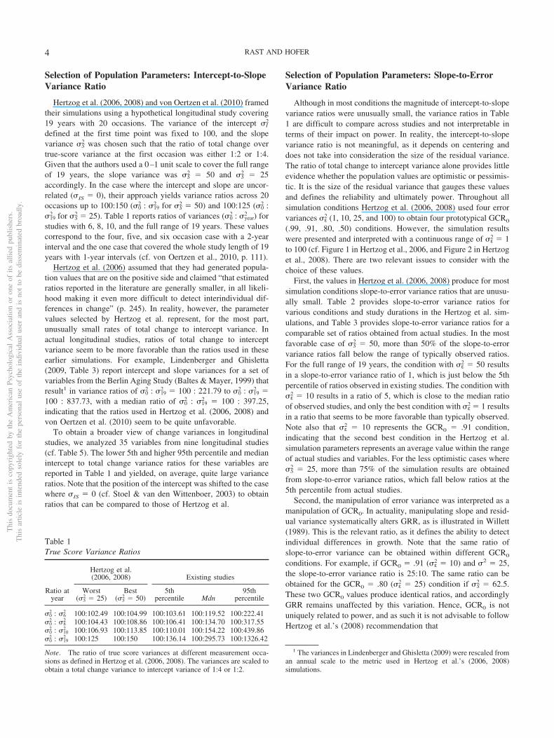
To obtain a broader view of change variances in longitudinalstudies, we analyzed 35 variables from nine longitudinal studies(cf. Table 5). The lower 5th and higher 95th percentile and medianintercept to total change variance ratios for these variables arereported in Table 1 and yielded, on average, quite large varianceratios. Note that the position of the intercept was shifted to the casewhere �IS � 0 (cf. Stoel & van den Wittenboer, 2003) to obtainratios that can be compared to those of Hertzog et al.
Selection of Population Parameters: Slope-to-ErrorVariance Ratio
Although in most conditions the magnitude of intercept-to-slopevariance ratios were unusually small, the variance ratios in Table1 are difficult to compare across studies and not interpretable interms of their impact on power. In reality, the intercept-to-slopevariance ratio is not meaningful, as it depends on centering anddoes not take into consideration the size of the residual variance.The ratio of total change to intercept variance alone provides littleevidence whether the population values are optimistic or pessimis-tic. It is the size of the residual variance that gauges these valuesand defines the reliability and ultimately power. Throughout allsimulation conditions Hertzog et al. (2006, 2008) used four errorvariances �ε
2 (1, 10, 25, and 100) to obtain four prototypical GCR0
(.99, .91, .80, .50) conditions. However, the simulation resultswere presented and interpreted with a continuous range of �ε
2 � 1to 100 (cf. Figure 1 in Hertzog et al., 2006, and Figure 2 in Hertzoget al., 2008). There are two relevant issues to consider with thechoice of these values.
First, the values in Hertzog et al. (2006, 2008) produce for mostsimulation conditions slope-to-error variance ratios that are unusu-ally small. Table 2 provides slope-to-error variance ratios forvarious conditions and study durations in the Hertzog et al. sim-ulations, and Table 3 provides slope-to-error variance ratios for acomparable set of ratios obtained from actual studies. In the mostfavorable case of �S
2 � 50, more than 50% of the slope-to-errorvariance ratios fall below the range of typically observed ratios.For the full range of 19 years, the condition with �ε
2 � 50 resultsin a slope-to-error variance ratio of 1, which is just below the 5thpercentile of ratios observed in existing studies. The condition with�ε
2 � 10 results in a ratio of 5, which is close to the median ratioof observed studies, and only the best condition with �ε
2 � 1 resultsin a ratio that seems to be more favorable than typically observed.Note also that �ε
2 � 10 represents the GCR0 � .91 condition,indicating that the second best condition in the Hertzog et al.simulation parameters represents an average value within the rangeof actual studies and variables. For the less optimistic cases where�S
2 � 25, more than 75% of the simulation results are obtainedfrom slope-to-error variance ratios, which fall below ratios at the5th percentile from actual studies.
Second, the manipulation of error variance was interpreted as amanipulation of GCR0. In actuality, manipulating slope and resid-ual variance systematically alters GRR, as is illustrated in Willett(1989). This is the relevant ratio, as it defines the ability to detectindividual differences in growth. Note that the same ratio ofslope-to-error variance can be obtained within different GCR0
conditions. For example, if GCR0 � .91 (�ε2 � 10) and �2 � 25,
the slope-to-error variance ratio is 25:10. The same ratio can beobtained for the GCR0 � .80 (�ε
2 � 25) condition if �S2 � 62.5.
These two GCR0 values produce identical ratios, and accordinglyGRR remains unaffected by this variation. Hence, GCR0 is notuniquely related to power, and as such it is not advisable to followHertzog et al.’s (2008) recommendation that
1 The variances in Lindenberger and Ghisletta (2009) were rescaled froman annual scale to the metric used in Hertzog et al.’s (2006, 2008)simulations.
Table 1True Score Variance Ratios
Ratio atyear
Hertzog et al.(2006, 2008) Existing studies
Worst(�S
2 � 25)Best
(�S2 � 50)
5thpercentile Mdn
95thpercentile
�02 : �6
2 100:102.49 100:104.99 100:103.61 100:119.52 100:222.41�0
2 : �82 100:104.43 100:108.86 100:106.41 100:134.70 100:317.55
�02 : �10
2 100:106.93 100:113.85 100:110.01 100:154.22 100:439.86�0
2 : �192 100:125 100:150 100:136.14 100:295.73 100:1326.42
Note. The ratio of true score variances at different measurement occa-sions as defined in Hertzog et al. (2006, 2008). The variances are scaled toobtain a total change variance to intercept variance of 1:4 or 1:2.
Thi
sdo
cum
ent
isco
pyri
ghte
dby
the
Am
eric
anPs
ycho
logi
cal
Ass
ocia
tion
oron
eof
itsal
lied
publ
ishe
rs.
Thi
sar
ticle
isin
tend
edso
lely
for
the
pers
onal
use
ofth
ein
divi
dual
user
and
isno
tto
bedi
ssem
inat
edbr
oadl
y.
4 RAST AND HOFER

At minimum, researchers should calculate estimates of GCR in theirstudy and evaluate whether it is sufficiently low to raise concernsabout power to detect random effects, which could be done to a crudeapproximation from the simulation results provided in this [Hertzog etal., 2008] study. Generically, our simulation indicates that GCRvalues under .90 are potentially problematic. (p. 560)
SST: Study Duration, Number of Occasions, andSpacing of Occasions
GRR is a function of �S2, �ε
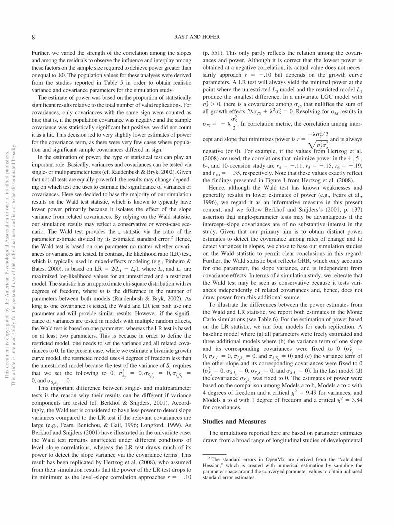
2, and SST whereby the latter isdetermined by study duration, number of waves, and relativespacing of occasions. In Hertzog et al. (2006, 2008) and vonOertzen et al. (2010), study duration and number of occasions areconfounded. The interval between occasions is constant at 2 yearsfor all conditions (except for the condition where all 20 occasionsare presented). As a result, only one of the three facets of SST wassystematically manipulated, rendering the results ambiguous withrespect to the impact of number of occasions on power. Althoughthe authors concluded from their simulations that number of oc-casions is a determining factor of power, it might as well be arguedthat it is not the number of measurement occasions but the studylength that matters. Given the discussion about the elements ofGRR, it is clear that study length has an important influence onGRR and on power because it impacts the size of SST. From theseprevious simulations it remains unknown whether power increaseddue to more measurement occasions or due to more time covered,or, and probably, both. These factors need to be manipulatedindependently in order to understand design decisions on power.Unfortunately, however, the Hertzog et al. results convey littleinformation about the interplay of power and design issues such asstudy length as well as number and spacing of measurementoccasions, which could have been illustrated even with unusualpopulation parameters. For example, if four waves are adminis-
tered over 6 years with �S2 � 50 and �ε
2 � 10, GRR is .22 (SST �0.05) but increases to .74 (SST � 0.56) if the same number ofmeasurement occasions cover the full study length of 19 years. Theincrease in GRR suggests that covering a longer period with thesame amount of waves has a strong effect on the ability to detectnonzero slope variances. GRR clearly indicates that it is notnecessarily the number of waves but also the time covered that canhave a beneficial effect on power. Figure 1 illustrates the effect ofstudy duration and number of waves with constant values of �S
2 �50 and �ε
2 � 10 on GRR. In this example, study length is scaled asa one-unit difference comprising 19 years (cf. Hertzog et al.,2006). Different numbers of measurement occasions are markedwith different symbols and range from three to 10 waves within agiven amount of time. The effect of increasing study length onGRR under equal numbers of measurement occasions is clearlyvisible. As more years are covered, GRR increases. At the sametime, increasing the number of measurement occasions within thesame study length increases GRR as well, and both manipulationsseem to have a unique effect on GRR.
So far, the above issues treat the impact of various componentsseparately. In reality, a number of interrelating factors that are
Table 2Total Change to Error Variance Ratios
Ratio at year �ε2 � 100 �ε
2 � 90 �ε2 � 75 �ε
2 � 50 �ε2 � 25 �ε
2 � 10 �ε2 � 1
Hertzog et al. (2006, 2008) with �S2 � 25
(�62 � �0
2)/�ε2 0.025 0.028 0.033 0.050 0.100 0.249 2.493
(�82 � �0
2)/�ε2 0.044 0.049 0.059 0.089 0.177 0.443 4.432
(�102 � �0
2)/�ε2 0.069 0.077 0.092 0.139 0.277 0.693 6.925
(�192 � �0
2)/�ε2 0.250 0.278 0.333 0.500 1 2.5 25
Hertzog et al. (2006, 2008) with �S2 � 50
(�62 � �0
2)/�ε2 0.050 0.055 0.066 0.100 0.199 0.499 4.986
(�82 � �0
2)/�ε2 0.089 0.098 0.118 0.177 0.355 0.886 8.864
(�102 � �0
2)/�ε2 0.139 0.154 0.185 0.277 0.554 1.385 13.850
(�192 � �0
2)/�ε2 0.500 0.556 0.667 1 2 5 50
Table 3Ratios at Percentiles From Existing Studies
Ratio at year 5th 25th Mdn 75th 95th
(�62 � �0
2)/�ε2 0.102 0.274 0.465 0.760 2.248
(�82 � �0
2)/�ε2 0.181 0.487 0.826 1.351 3.997
(�102 � �0
2)/�ε2 0.283 0.761 1.291 2.110 6.246
(�192 � �0
2)/�ε2 1.022 2.748 4.661 7.618 22.547
Length of Study
GR
R
0 2/19 4/19 6/19 8/19 10/19 12/19 14/19 16/19 18/19
0.0
0.2
0.4
0.6
0.8
1.0 Measurement occasions:
= 3= 4= 5
= 7=10
Figure 1. The effect of study length and number of measurement occa-sions on growth rate reliability (GRR). The slope variance is �S
2 � 50, andthe error variance is �ε
2 � 10. Study length is scaled as a one-unit differencecomprising 19 years (cf. Hertzog et al. 2006).
Thi
sdo
cum
ent
isco
pyri
ghte
dby
the
Am
eric
anPs
ycho
logi
cal
Ass
ocia
tion
oron
eof
itsal
lied
publ
ishe
rs.
Thi
sar
ticle
isin
tend
edso
lely
for
the
pers
onal
use
ofth
ein
divi
dual
user
and
isno
tto
bedi
ssem
inat
edbr
oadl
y.
5LONGITUDINAL STUDY DESIGN: OPTIMIZING POWER

described in GRR contribute to power. GCR0, defined by the errorvariance, is one of them and cannot be considered independently ofother values, as it reflects only one facet of a number of factors thatinfluence GRR. Figure 2, which mirrors the power plot of Hertzoget al. (2008, Figure 3), illustrates this relation among �S
2, GCR0
(�ε2), and four designs. It is clear that GCR0 is not uniquely related
to power or GRR because altering �S2 also changes the slope-to-
error variance ratio, and in each of the four designs SST is differentas well. As described previously, the same GRR value is obtainedin a number of different GCR0 conditions, and the same GCR0
condition can result in almost any GRR or power value. Forexample, a constant value of GCR0 � .91 yields GRR values thatrange form 0 to .36 in the four-occasions design or from 0 to .90in the 10-occasions design. Accordingly, power to detect slopevariances can take almost any value within a given GCR0 condi-tion. Figure 2 clearly illustrates that the only value that is uniquelyrelated to power is GRR, and it also shows that power is a functionof GRR. What remains unknown, however, is the nature of thefunction that relates power to GRR. Also, the curves illustrate theimpact of study duration with equally spaced measurement occa-sions. However, Hertzog et al. (2006, 2008) and von Oertzen et al.(2010) did not indicate the unique impact of study duration,number of measurement occasions, and interval size on GRR.
Aim of the Study
The present study evaluates the power to detect variances andcovariances among rates of change in growth curve models usingMonte Carlo simulations. We base these simulations on a range ofsensible population values from a number of different longitudinalstudies comprising early and late life periods and varying insample size, number of waves, interval lengths, overall studyfollow-up, variables, heterogeneity of baseline age, and othercharacteristics of the participants. We examine power across sev-eral variable domains that are often the focus within developmen-
tal and aging psychology: cognition, affect, physical functioning,and dimensions of psychopathology. Together these studies pro-vide a basis for estimating power as well as a realistic range ofpopulation values for further simulation studies.
Our aim is to understand the effect of critical design parameterson power to detect individual differences in growth. GRR, themeasure of the reliability of the growth rate proposed by Willett(1989), is used as an index of power to detect individual differ-ences in change but also as a guide to identify the interplay amongits elements, slope variance, error variance, number and spacing ofwaves, and study length. Of special interest are the variables thatconstitute SST, as they are under the control of the researcherconducting a longitudinal study and can be used to optimize powerin the early phases of such studies.
Method
Latent Growth Curve Modeling
Our analyses are based on a bivariate linear growth curve (LGC)model where we observe a set of repeated observations on twovariables Y and X for individual i in a longitudinal setting with severalwaves. Let yi � �y1, y2, . . . , yWi
�� denote the response on Y andxi � �x1, x2, . . . , xWi
�� denote the response on X for individual i. Theresponses are observed according to a set of waves wi � (1, 2, 3, . . . ,Wi)=, where Wi is the total number of waves for individual i, which donot need to be the same for all individuals. A general expression fora time-structured latent growth curve model for two variables yi andxi then is
yi � �yi�yi � �yi
xi � �xi�xi � �xi, (3)
where � is the (Wi � p) factor loading matrix with number of rowsequal to Wi and where the number of columns is equal to the
4 occasions(SST=0.06)
Slope Variance (σS2)
0 20 60 100
0.0
0.2
0.4
0.6
0.8
1.0
GR
R
5 occasions(SST=0.11)
Slope Variance (σS2)
0 20 60 100
6 occasions(SST=0.19)
Slope Variance (σS2)
0 20 60 100
10 occasions(SST=0.91)
Slope Variance (σS2)
0 20 60 100
GCR σε2
0.99 10.91 100.8 250.5 100
Figure 2. Growth rate reliability (GRR) as a function of slope variance (�S2) among different numbers of
measurement occasions. The four lines are based on four error variances. The figure parallels the power plotsin Hertzog et al. (2008, Figure 3) and shows how growth curve reliability (GCR) is related to GRR. Fouroccasions cover a study duration of 6 years, 5 occasions cover 8 years, 6 occasions cover 10, and 10 occasionscover 18 years. SST � total sum of squared deviations of time points.
Thi
sdo
cum
ent
isco
pyri
ghte
dby
the
Am
eric
anPs
ycho
logi
cal
Ass
ocia
tion
oron
eof
itsal
lied
publ
ishe
rs.
Thi
sar
ticle
isin
tend
edso
lely
for
the
pers
onal
use
ofth
ein
divi
dual
user
and
isno
tto
bedi
ssem
inat
edbr
oadl
y.
6 RAST AND HOFER

number of factors or growth parameters (p) estimated in the model(here p � 2 for each variable). The vector � captures the randomeffects particular to individual i in the intercept and slope, and �represents a vector of residuals. We follow standard assumptionswhere E(�) � 0 and COV(�, �) � 0. Further, let E(�) � �,COV(�, �) � �, and COV(�, �) � �.
In the bivariate LGC model (cf. MacCallum et al., 1997; Tisak &Meredith, 1990, for the general multivariate case) Y and X are mod-eled simultaneously, which is expressed in the means and covariancematrix
� � ��
� � ���′ � �. (4)
The vector of means � has 2p elements; in the case where weestimate two intercept and two slope parameters, the elements 1and 3 in � pertain to the intercept and the elements 2 and 4 capturethe slope of Y and X. � defines the loadings (i.e., intercepts andslopes) for both sets of variables with the dimension 2W � 2p, andthe 2p � 2p covariance matrix � is unstructured, leaving the(co-)variances unconstrained:
� ��1 �y0 0 0
1 �y1 0 0
É É É É
1 �yW 0 0
0 0 1 �x0
0 0 1 �x1
É É É É
0 0 1 �xW
�, � ���Iy
2
�SyIy�Sy
2
�IxIy�IxSy
�Ix
2
�SxIy�SxSy
�SxIx�Sx
2�.
To set the intercept at the first wave, we assign �y0and �x0
thevalue 0. The loadings �w may take different scales; usually theyare assigned values that reflect the interval of the measurementoccasions, but they may be scaled to alternative metrics as well asbe individually time-varying. Note that here both variables aremeasured at the same occasions and, hence, �y � �x.
To account for dependencies across measurements within eachwave, we relaxed the condition of uncorrelated residuals andallowed occasion-specific covariances among the residuals acrossY and X. The residual covariance matrix with equality constraintsacross occasion-specific residual covariances is defined as
� ����y
2
0 Ì
É É ��y
2
��x�y0 . . . ��x
2
É ��x�y0 É Ì
0 . . . ��x�y0 . . . ��x
2
�.
This bivariate growth model is represented in Figure 3, and itwas used to both estimate parameter values from a set of longitu-dinal studies and served as the basis for all simulations.
Power Estimation
Statistical power is defined as the probability of correctly rejectingthe null hypothesis when it is false (Cohen, 1988), which is repre-
sented as power () � 1 � , where represents the probability ofa Type II error. Statistical power depends on a number of factors, suchas the Type I error rate, sample, and effect size. In the present workwe will use the commonly applied values of � .05 to definestatistical significance and values of � .80 to define sufficientpower.
To assess the power to detect variance in slopes ��Sx
2 , �Sy
2 � andcovariances among slopes (�SySx
), in a first step we estimated theactual power for these parameters in a number of current longitudinalstudies. All parameters were based on the same bivariate longitudinalgrowth curve model described in Equation 4 and depicted in Figure 3.The estimates for each combination of variables upon which thesimulations were based are reported in Table 5. We used Monte Carlosimulations to estimate the power for each variable combinationwithin the reported longitudinal studies and the sample size needed toobtain power of at least � .80. For all analyses, the extraction ofpopulation values and the estimation of power for different conditionswere based on an annual time scale where one unit represents 1 year.The choice of an annual time scale is arbitrary and does not change thepower estimates, but it places the population parameters on a com-monly used metric, which facilitates their interpretation and compar-ison to other studies.
In a second step, we systematically varied the number of waves, theinterval between waves, the total duration of the study, and the size ofthe error and slope variance in order to obtain different GRR values.
Figure 3. The bivariate latent growth curve model that was used toextract parameter values from existing longitudinal studies. This modelwas also used to obtain power estimates by means of Monte Carlo simu-lations.
Thi
sdo
cum
ent
isco
pyri
ghte
dby
the
Am
eric
anPs
ycho
logi
cal
Ass
ocia
tion
oron
eof
itsal
lied
publ
ishe
rs.
Thi
sar
ticle
isin
tend
edso
lely
for
the
pers
onal
use
ofth
ein
divi
dual
user
and
isno
tto
bedi
ssem
inat
edbr
oadl
y.
7LONGITUDINAL STUDY DESIGN: OPTIMIZING POWER
Further, we varied the strength of the correlation among the slopesand among the residuals to observe the influence and interplay amongthese factors on the sample size required to achieve power greater thanor equal to .80. The population values for these analyses were derivedfrom the studies reported in Table 5 in order to obtain realisticvariance and covariance parameters for the simulation study.
The estimate of power was based on the proportion of statisticallysignificant results relative to the total number of valid replications. Forcovariances, only covariances with the same sign were counted ashits; that is, if the population covariance was negative and the samplecovariance was statistically significant but positive, we did not countit as a hit. This decision led to very slightly lower estimates of powerfor the covariance term, as there were very few cases where popula-tion and significant sample covariances differed in sign.
In the estimation of power, the type of statistical test can play animportant role. Basically, variances and covariances can be tested viasingle- or multiparameter tests (cf. Raudenbush & Bryk, 2002). Giventhat not all tests are equally powerful, the results may change depend-ing on which test one uses to estimate the significance of variances orcovariances. Here we decided to base the majority of our simulationresults on the Wald test statistic, which is known to typically havelower power primarily because it isolates the effect of the slopevariance from related covariances. By relying on the Wald statistic,our simulation results may reflect a conservative or worst-case sce-nario. The Wald test provides the z statistic via the ratio of theparameter estimate divided by its estimated standard error.2 Hence,the Wald test is based on one parameter no matter whether covari-ances or variances are tested. In contrast, the likelihood ratio (LR) test,which is typically used in mixed-effects modeling (e.g., Pinheiro &Bates, 2000), is based on LR � 2(L1 � L0), where L0 and L1 aremaximized log-likelihood values for an unrestricted and a restrictedmodel. The statistic has an approximate chi-square distribution with mdegrees of freedom, where m is the difference in the number ofparameters between both models (Raudenbush & Bryk, 2002). Aslong as one covariance is tested, the Wald and LR test both use oneparameter and will provide similar results. However, if the signifi-cance of variances are tested in models with multiple random effects,the Wald test is based on one parameter, whereas the LR test is basedon at least two parameters. This is because in order to define therestricted model, one needs to set the variance and all related cova-riances to 0. In the present case, where we estimate a bivariate growthcurve model, the restricted model uses 4 degrees of freedom less thanthe unrestricted model because the test of the variance of Sy requiresthat we set the following to 0: �Sy
2 � 0, �SyIy� 0, �IxSy
�
0, and �SxSy� 0.
This important difference between single- and multiparametertests is the reason why their results can be different if variancecomponents are tested (cf. Berkhof & Snijders, 2001). Accord-ingly, the Wald test is considered to have less power to detect slopevariances compared to the LR test if the relevant covariances arelarge (e.g., Fears, Benichou, & Gail, 1996; Longford, 1999). AsBerkhof and Snijders (2001) have illustrated in the univariate case,the Wald test remains unaffected under different conditions oflevel–slope correlations, whereas the LR test draws much of itspower to detect the slope variance via the covariance terms. Thisresult has been replicated by Hertzog et al. (2008), who assumedfrom their simulation results that the power of the LR test drops toits minimum as the level–slope correlation approaches r � �.10
(p. 551). This only partly reflects the relation among the covari-ances and power. Although it is correct that the lowest power isobtained at a negative correlation, its actual value does not neces-sarily approach r � �.10 but depends on the growth curveparameters. A LR test will always yield the minimal power at thepoint where the unrestricted L0 model and the restricted model L1
produce the smallest difference. In a univariate LGC model with�S
2 � 0, there is a covariance among �IS that nullifies the sum ofall growth effects 2��IS � �2�S
2 � 0. Resolving for �IS results in
�IS � � ��S
2
2. In correlation metric, the correlation among inter-
cept and slope that minimizes power is r ����S
2 ⁄ 2
��I2�S
2and is always
negative (or 0). For example, if the values from Hertzog et al.(2008) are used, the correlations that minimize power in the 4-, 5-,6-, and 10-occasion study are r4 � �.11, r5 � �.15, r6 � �.19,and r10 � �.35, respectively. Note that these values exactly reflectthe findings presented in Figure 1 from Hertzog et al. (2008).
Hence, although the Wald test has known weaknesses andgenerally results in lower estimates of power (e.g., Fears et al.,1996), we regard it as an informative measure in this presentcontext, and we follow Berkhof and Snijders’s (2001, p. 137)assertion that single-parameter tests may be advantageous if theintercept–slope covariances are of no substantive interest in thestudy. Given that our primary aim is to obtain distinct powerestimates to detect the covariance among rates of change and todetect variances in slopes, we chose to base our simulation studieson the Wald statistic to permit clear conclusions in this regard.Further, the Wald statistic best reflects GRR, which only accountsfor one parameter, the slope variance, and is independent fromcovariance effects. In terms of a simulation study, we reiterate thatthe Wald test may be seen as conservative because it tests vari-ances independently of related covariances and, hence, does notdraw power from this additional source.
To illustrate the differences between the power estimates fromthe Wald and LR statistic, we report both estimates in the MonteCarlo simulations (see Table 6). For the estimation of power basedon the LR statistic, we ran four models for each replication. Abaseline model where (a) all parameters were freely estimated andthree additional models where (b) the variance term of one slopeand its corresponding covariances were fixed to 0 ��Sy
2 �0, �SyIy
� 0, �IxSy� 0, and �SxSy
� 0� and (c) the variance term ofthe other slope and its corresponding covariances were fixed to 0��Sx
2 � 0, �SxIy� 0, �SxSy
� 0, and �SxIx� 0�. In the last model (d)
the covariance �SxSywas fixed to 0. The estimates of power were
based on the comparison among Models a to b, Models a to c with4 degrees of freedom and a critical �2 � 9.49 for variances, andModels a to d with 1 degree of freedom and a critical �2 � 3.84for covariances.
Studies and Measures
The simulations reported here are based on parameter estimatesdrawn from a broad range of longitudinal studies of developmental
2 The standard errors in OpenMx are derived from the “calculatedHessian,” which is created with numerical estimation by sampling theparameter space around the converged parameter values to obtain unbiasedstandard error estimates.
Thi
sdo
cum
ent
isco
pyri
ghte
dby
the
Am
eric
anPs
ycho
logi
cal
Ass
ocia
tion
oron
eof
itsal
lied
publ
ishe
rs.
Thi
sar
ticle
isin
tend
edso
lely
for
the
pers
onal
use
ofth
ein
divi
dual
user
and
isno
tto
bedi
ssem
inat
edbr
oadl
y.
8 RAST AND HOFER

and aging-related change. Design characteristics of the includedlongitudinal studies are provided in Table 4, and descriptive sta-tistics are reported in Table 5. Bivariate linear growth modelsdescribed in Equation 4 were analyzed for each set of outcomesand were used to provide a range of realistic values on which tobase an evaluation of power to detect variance in linear slopes andbivariate associations in linear rates of change.
All of the actual longitudinal studies used in this article hadincomplete data due to study attrition. In addition, in longitudinalstudies of aging, this attrition is related primarily to dropout due todeath. Incomplete data were estimated under the assumption thatthe data are at least missing at random (MAR; where the proba-bility of missing information is related to covariates and previouslymeasured outcomes). Such methods are in regular usage in anal-ysis of longitudinal studies. However, attrition in studies of agingis often nonrandom, or selective, in that it is likely to result frommortality or declining physical and mental functioning of theparticipants over the period of observation. In the case ofmortality-related dropout, the MAR assumption is likely to beproblematic unless age at death is included in the model to accountfor population selection.
The parameter estimates were obtained via full informationmaximum likelihood (FIML). We report only linear growth mod-els with fixed time-in-study intervals as the time basis and onlymodels with adequate model fit according to the comparative fitindex (above .95) and the root-mean-square error of approximation(below .08; Browne & Cudeck, 1993; MacCallum, Browne, &Sugawara, 1996). Estimates were based on annual rates of changewith the intercept specified at baseline. We refrained from usingthe unit scale transformation applied by Hertzog et al. (2006; andlater studies), which covers 19 years, because it provides estimatesthat are uncommon, as most researchers scale change in years. Thepurpose of Table 5 is also to provide an array of actual populationvalues in the most common format. As pointed out earlier, allvariance and covariance estimates can be rescaled to be on othertime metrics, such as the 0–1 unit scale adopted by these earliersimulation studies, with GRR and power being invariant to suchrescaling. Note that our primary aim in the parameter extractionwas to obtain a range of realistic values for later use as populationvalues in simulation studies. Hence, we chose to remain with theFIML in order to make full use of the sample sizes, and we did notinclude higher order terms to capture curvilinear changes over timein the few cases where this was indicated.
All of the power estimates in Table 6 were based on 10,000replications. To compute and plot the required sample size forpower of at least � .80 for given population values, we used aniterative approach whereby the final iterations approached � .80by steps of N � 10 to ensure sufficient precision. The figures weregenerated with 5,000 replications in the final iteration steps. Allanalyses made use of the software package R (R DevelopmentCore Team, 2012), where we relied on the mvrnorm function fromthe MASS package (Venables & Ripley, 2002) to generate randombivariate samples with the structure given in Equations 4 and 5.The statistical analysis of the LGC models was performed with thefreely available structural equation modeling software packageOpenMx (Version 1.2.3; Boker et al., 2011). To check the consis-tency of the power estimates based on the Wald statistic, we reranall models (i.e., data generation and estimation) within the MonteCarlo facility of Mplus (L. K. Muthén & Muthén, 2010). The
results from both software packages resulted in close to identicalpower and sample size estimates. To speed up computing time, weconducted all analyses in R on Nestor, a capability cluster gearedtoward large parallel jobs provided by WestGrid and Compute/Calcul Canada. Sample scripts used in this simulation study areavailable in the supplemental materials and for integration in R orMplus.
Results
Power Estimates for Actual Study Values
A sample of longitudinal developmental and aging studies wasused as a foundation to evaluate power to detect variance in, andassociations among, rates of change. Table 5 provides descriptivestatistics and estimated values from bivariate growth curve modelsfor a variety of outcomes, including cognitive, physical function-ing, and mental health variables. In few cases, particularly instudies with more waves and longer follow-up, quadratic trendswere indicated. However, all reported estimates are based on LGCmodels in order to permit evaluation of linear slope associationsand to provide a consistent basis for obtaining LGC parameters forsimulation purposes. The values from Table 5 provide the basis forestimating power for particular combinations of variables withinactual studies but also for extrapolating to a range of effect sizes,sample sizes, and slope reliabilities. Notably, 95% of the slope-to-error variance in these longitudinal studies ranged from 1:14 to1:478. The average ratio was 1:335 and the median was 1:81,indicating that the error variance was 81 times larger relative to theslope variance. Accordingly, 95% of GRR ranged from .07 to .71,with a median GRR of .36. For these same variables, 95% of GCR0
values ranged from .33 to .90, with a median of .68.Based on the results of Table 5, Table 6 provides standardized
estimates of associations among slopes and power to detect linearslope variances and covariances in bivariate combinations of out-comes. Results from Monte Carlo simulations using both Wald andLR statistics are reported.
Covariance among slopes. The correlations among rates ofchange ranged from �.57 (Victoria Longitudinal Study [VLS];simple reaction time with Identical Pictures [IPic]) to .03 (VLS;Social Activities with IPic) to .89 (Australian Child to AdultDevelopment Study [ACAD]; D with SA), with an average, abso-lute correlation of r � |.52|. Power and the sample size needed toobtain power of at least .80 was largely dependent on two factors:the magnitude of the correlation among the slopes (i.e., effect size)and the magnitude of GRR. If any one of these factors was small,sufficient power ( � .80) to detect the covariance was onlyachieved with large sample sizes. For example, in the SeattleLongitudinal Study, the sample size was comparable among thefive sets of variable pairs, but the power ranged from .09 to 1.0.Power estimates for the covariances appeared to be related to theGRR values of the respective variables. For example, the power todetect the correlation among variables including the Physical Ac-tivity from Life Complexity Scale (PHY; GRR .03) was alwaysvery low, and there was virtually no chance to detect correlationsinvolving the PHY variable with the available sample size. In turn,the somewhat stronger correlation among Delayed Word Recall(DWR) and Number Comparison in the same study had sufficientpower to be detected. Given the simulation results, 240 partici-
Thi
sdo
cum
ent
isco
pyri
ghte
dby
the
Am
eric
anPs
ycho
logi
cal
Ass
ocia
tion
oron
eof
itsal
lied
publ
ishe
rs.
Thi
sar
ticle
isin
tend
edso
lely
for
the
pers
onal
use
ofth
ein
divi
dual
user
and
isno
tto
bedi
ssem
inat
edbr
oadl
y.
9LONGITUDINAL STUDY DESIGN: OPTIMIZING POWER

Tab
le4
Des
crip
tion
ofL
ongi
tudi
nal
Stud
ies
and
Sele
cted
Var
iabl
es
Stud
ySt
art
year
N(T
ime
1)
Age
inye
ars
(Tim
e1)
Occ
asio
nin
terv
al
Num
ber
ofoc
casi
ons
Typ
esa
mpl
eM
easu
rem
ent
Ref
eren
ces
Aus
tral
ian
Chi
ldto
Adu
ltD
evel
opm
ent
Stud
y(A
CA
D)
1991
578
4–19
4.5,
7.5,
11.3
4H
ealth
,ed
ucat
ion,
and
fam
ilyse
rvic
eag
enci
esth
atpr
ovid
edse
rvic
esto
child
ren
with
inte
llect
ual
defi
cits
ofal
lle
vels
Dev
elop
men
tal
Beh
avio
rC
heck
list:
Dis
rupt
ive/
Ant
isoc
ial
(D);
Self
-A
bsor
bed
(SA
);C
omm
unic
atio
nD
istu
rban
ce(C
D);
Anx
iety
(A);
Soci
alR
elat
ing
(SR
)
Ein
feld
&T
onge
(199
2,19
95,
2002
)
Eng
lish
Lon
gitu
dina
lSt
udy
ofA
gein
g(E
LSA
)
2002
12,1
0049
2.3,
4.12
,6.
194
Rep
rese
ntat
ive
Del
ayed
Wor
dR
ecal
l(D
WR
);Pr
ospe
ctiv
eM
emor
y(P
M);
Ani
mal
Flue
ncy
(AF)
Ban
kset
al.
(200
8,20
10);
Hup
pert
etal
.(2
006)
;R
oth
etal
.(1
986)
Hea
lthan
dR
etir
emen
tSt
udy
(HR
S)an
dA
HE
AD
1992
12,6
0050
–60
1.94
,4.
10,
6.03
,8.
045
Nat
iona
lsa
mpl
e,m
inor
ities
over
sam
pled
Imm
edia
te(I
WR
S)an
dD
elay
ed(D
WR
S)W
ord
Rec
all;
Subt
ract
7s(S
S);D
epre
ssiv
eSy
mpt
oms
(CE
SD)
Just
er&
Suzm
an(1
995)
;R
adlo
ff(1
977)
Lon
gitu
dina
lA
ging
Stud
yA
mst
erda
m(L
ASA
)19
92–1
993
3,10
755
3.11
,6.
08,
9.03
,13
.15
5St
ratif
ied
rand
omsa
mpl
eof
urba
nan
dru
ral
mun
icip
alre
gist
ries
Alp
habe
tCod
ing
Tas
k(A
lC);
Min
i-M
enta
lSta
teE
xam
inat
ion
(MM
SE);
Rav
enC
olou
red
Prog
ress
ive
Mat
rices
(RC
PM)
Fols
tein
etal
.(1
975)
;H
uism
anet
al.
(201
1);
Picc
inin
&R
abbi
tt(1
999)
;R
aven
etal
.(1
995,
Sect
ion
2);
Sava
ge(1
984)
Lon
gB
each
Lon
gitu
dina
lSt
udy
(LB
LS)
1978
509
55–8
73.
28,
6.18
,8.
414
Rec
ruite
dfr
omhe
alth
mai
nten
ance
orga
niza
tion
Let
ter
and
Num
ber
Seri
es(R
eas)
;ST
AM
AT
Rec
ogni
tion
Voc
abul
ary
(VC
B);
Com
posi
teof
Patte
rn,
Num
ber,
and
Let
ter
Com
pari
son
(SPD
)
Scha
ie(1
985)
;Z
elin
ski
&B
urnr
ight
(199
7)
Ori
gins
ofV
aria
nce
inth
eO
ld-O
ld:
Oct
ogen
aria
nT
win
s(O
CT
O-T
win
)
1990
702
802.
06,
4.07
,6.
04,
8.03
5Sw
edis
hT
win
Reg
istr
yM
emor
y-in
-Rea
lity
Free
Rec
all
(MiR
);D
igit
Sym
bol
Subs
titut
ion
Tes
t(D
ST);
Koh
’sB
lock
Des
ign
(BlK
);Pe
akE
xpir
ator
yV
olum
e(P
EF)
Ced
erlö
f&
Lor
ich
(197
8);
Coo
ket
al.
(199
5);
Joha
nsso
net
al.
(199
9,20
04);
McC
lear
net
al.
(199
7);
Wec
hsle
r(1
991)
Seat
tleL
ongi
tudi
nal
Stud
y(S
LS)
1984
557.
00,
13.6
3,21
.00
4H
ealth
mai
nten
ance
orga
niza
tion;
sequ
entia
lde
sign
Num
ber
Com
pari
son
(NC
);W
ord
Seri
esR
easo
ning
Tes
t(W
ST);
Wor
dFl
uenc
y(W
FT);
Del
ayed
Wor
dR
ecal
l(D
WR
);Ph
ysic
alA
ctiv
ityfr
omL
ife
Com
plex
itySc
ale
(PH
Y)
Eks
trom
etal
.(1
976)
;Sc
haie
(198
5);
Thu
rsto
ne&
Thu
rsto
ne(1
949)
Vic
tori
aH
ealth
yY
outh
Surv
ey(V
HY
S)20
0366
412
–18
2.08
,4.
05,
6.83
4R
ando
mdi
git
dial
ing
ofG
reat
erV
icto
ria
area
Brie
fC
hild
and
Fam
ilyPh
one
Inte
rvie
w(B
CFP
I):A
nxie
ty(A
nx);
Dep
ress
ion
(Dep
);O
ppos
ition
alD
efia
nce
(OpD
);Fr
iend
s’po
sitiv
ean
dne
gativ
eac
tiviti
es(F
rAc)
Bar
nes
etal
.(2
009)
;C
unni
ngha
met
al.
(200
9)
Vic
tori
aL
ongi
tudi
nal
Stud
y(V
LS)
55–8
53.
06,
6.08
,9.
504
Com
mun
ityvo
lunt
eers
;se
quen
tial
desi
gnSi
mpl
ere
actio
ntim
e(S
RT
);W
ord
Rec
all
(WR
C);
Iden
tical
Pict
ures
(IPi
c);
Phys
ical
Act
iviti
es(P
A);
Soci
alA
ctiv
ities
(SA
)
Dix
on&
deFr
ias
(200
4);
Hul
tsch
etal
.(1
998,
1999
)
Thi
sdo
cum
ent
isco
pyri
ghte
dby
the
Am
eric
anPs
ycho
logi
cal
Ass
ocia
tion
oron
eof
itsal
lied
publ
ishe
rs.
Thi
sar
ticle
isin
tend
edso
lely
for
the
pers
onal
use
ofth
ein
divi
dual
user
and
isno
tto
bedi
ssem
inat
edbr
oadl
y.
10 RAST AND HOFER

Tab
le5
Des
crip
tive
Stat
isti
csan
dE
stim
ated
Val
ues
Fro
mB
ivar
iate
Gro
wth
Cur
veM
odel
sfo
rSt
udie
sB
ased
onT
hree
,F
our,
and
Fiv
eW
aves
Stud
yy
xN
�Iy2
�Sy2
�Ix2
�Sx2
�Iy
Sy
�Iy
Sx
�Iy
Sy
�SyI
x�
SyS
x�
IxSx
��
y2�
�x2
��
y�x
Wav
esL
engt
h
OC
TO
BlK
MiR
486
39.6
300.
531
4.02
60.
138
�0.
694
5.81
70.
625
0.25
20.
162
0.27
49.
203
1.89
40.
510
34.
07O
CT
OD
STM
iR43
397
.289
1.63
83.
533
0.14
1�
2.31
79.
110
1.16
2�
0.17
00.
267
0.30
621
.106
1.99
50.
512
34.
07O
CT
OPE
FD
ST36
697
61.8
0449
.436
98.9
671.
403
�36
1.76
732
9.60
13.
343
�17
.701
3.05
9�
2.79
123
43.1
8622
.478
0.28
93
4.07
LA
SAA
lCM
MSE
2,57
152
.440
0.10
93.
325
0.05
90.
412
9.90
01.
037
0.22
60.
036
0.35
15.
417
2.79
50.
201
36.
08L
ASA
RC
PMA
lC2,
430
10.9
830.
022
50.1
980.
101
0.10
516
.516
0.13
10.
300
0.02
50.
115
5.19
95.
326
�0.
010
36.
08A
CA
DA
CD
506
6.29
10.
039
13.2
010.
072
�0.
259
4.62
0�
0.09
6�
0.17
50.
026
0.39
83.
867
6.34
11.
941
411
.3A
CA
DA
SR50
66.
270
0.03
87.
348
0.03
5�
0.25
52.
949
�0.
031
�0.
048
0.01
4�
0.07
63.
877
4.66
01.
324
411
.3A
CA
DC
DD
506
13.1
640.
070
73.5
720.
300
�0.
384
18.6
62�
0.74
5�
0.57
70.
114
�2.
438
6.34
821
.993
5.95
74
11.3
AC
AD
CD
SA50
613
.192
0.07
188
.168
0.26
4�
0.39
515
.392
�0.
786
�0.
393
0.11
1�
1.84
96.
341
21.1
916.
030
411
.3A
CA
DD
SA50
673
.610
0.29
987
.869
0.25
9�
2.45
432
.880
�2.
020
�0.
987
0.24
8�
1.81
522
.034
21.3
1913
.351
411
.3A
CA
DD
SR50
673
.366
0.29
67.
352
0.03
4�
2.42
57.
747
�0.
032
�0.
203
0.05
3�
0.07
422
.094
4.66
33.
989
411
.3A
CA
DSA
SR50
687
.962
0.25
67.
290
0.03
5�
1.79
415
.919
�0.
157
�0.
340
0.04
9�
0.07
621
.292
4.67
64.
524
411
.3E
LSA
DW
RA
F11
,017
261.
696
1.41
024
63.0
4615
.530
1.22
754
9.45
421
.609
7.85
42.
175
44.3
0418
2.75
816
44.8
7850
.906
46.
19E
LSA
DW
RPM
10,9
8725
9.86
81.
475
112.
989
1.01
80.
900
111.
142
0.43
30.
675
0.63
7�
2.74
918
2.87
723
0.52
47.
914
46.
19E
LSA
AF
PM10
,988
2436
.489
15.4
6411
3.48
20.
978
40.2
0828
9.29
4�
1.48
98.
825
1.42
6�
2.82
016
48.5
4223
0.51
427
.965
46.
19L
BL
SR
eas
SPD
504
122.
904
0.35
871
0.29
31.
702
0.03
422
1.45
32.
600
3.14
50.
530
5.92
812
.886
79.4
292.
914
48.
41L
BL
SR
eas
VC
B59
512
6.21
10.
324
103.
922
0.39
4�
0.59
079
.494
0.91
4�
1.35
90.
248
�0.
272
12.8
5512
.788
0.31
44
8.41
LB
LS
SPD
VC
B50
873
4.64
61.
713
90.6
870.
413
9.40
616
9.85
77.
156
1.86
60.
486
0.56
980
.464
12.8
844.
167
48.
41SL
SD
WR
WFT
765
1400
.770
1.53
913
192.
938
13.9
535.
726
2448
.552
20.1
50�
1.56
33.
747
�7.
692
540.
669
3208
.648
24.5
994
21SL
SD
WR
NC
766
1395
.275
1.48
021
05.7
451.
691
8.33
775
2.31
05.
176
10.9
300.
852
�14
.092
541.
774
736.
465
75.0
614
21SL
SW
FTN
C78
313
132.
604
13.0
0021
03.6
261.
598
12.0
4623
80.8
493.
942
32.7
632.
940
�13
.618
3220
.428
743.
690
172.
179
421
SLS
PHY
NC
761
54.1
250.
007
2055
.156
1.59
0�
0.44
472
.746
1.62
8�
1.01
0�
0.04
5�
14.1
7563
.798
760.
697
2.25
74
21SL
SPH
YD
WR
749
53.3
520.
005
1406
.833
1.54
6�
0.40
064
.853
1.24
1�
1.61
70.
027
5.01
664
.186
546.
304
2.15
34
21V
HY
SA
nxD
ep66
23.
451
0.04
43.
565
0.04
7�
0.10
21.
890
�0.
039
0.03
50.
022
�0.
100
3.22
03.
125
0.92
64
6.83
VH
YS
Anx
OpD
662
3.44
10.
042
3.21
90.
029
�0.
096
1.24
0�
0.05
00.
045
0.01
5�
0.10
33.
231
2.24
50.
609
46.
83V
HY
SD
epO
pD66
23.
583
0.04
83.
220
0.02
9�
0.10
22.
061
�0.
066
�0.
034
0.02
3�
0.10
33.
115
2.24
20.
868
46.
83V
HY
SA
nxFr
Ac
662
3.44
60.
042
9.60
00.
205
�0.
098
1.73
1�
0.34
3�
0.27
50.
055
�0.
112
3.23
323
.633
0.23
84
6.83
VH
YS
Dep
FrA
c66
23.
577
0.04
89.
636
0.20
5�
0.10
51.
096
�0.
301
�0.
263
0.03
6�
0.11
73.
120
23.6
250.
052
46.
83V
HY
SO
pDFr
Ac
662
3.22
10.
029
9.60
20.
205
�0.
104
0.59
7�
0.02
4�
0.12
80.
023
�0.
106
2.24
623
.620
�0.
069
46.
83V
LS
SRT
WR
C52
128
71.9
3227
.380
14.0
990.
056
41.8
31�
62.2
96�
3.54
6�
5.84
9�
0.59
10.
250
2816
.220
4.99
2�
5.29
94
9.5
VL
SSR
TIP
ic52
128
39.3
4032
.226
28.7
990.
838
42.7
21�
139.
087
�2.
772
�1.
572
�2.
940
�0.
563
2861
.373
17.4
72�
21.3
664
9.5
VL
SW
RC
IPic
522
14.1
640.
055
28.9
890.
850
0.23
910
.101
�0.
418
0.30
10.
074
�0.
656
5.01
017
.356
�0.
345
49.
5V
LS
SAIP
ic50
433
.556
0.17
628
.020
0.89
8�
0.32
27.
423
�0.
284
�0.
044
0.01
3�
0.73
112
.874
17.4
94�
0.83
34
9.5
VL
SSA
SRT
503
33.6
110.
179
2742
.526
27.3
23�
0.32
7�
17.3
042.
364
�2.
138
�1.
051
23.0
2912
.843
2769
.302
8.73
64
9.5
VL
SPA
SRT
503
17.8
540.
090
2742
.510
27.1
30�
0.28
9�
33.7
591.
217
�2.
792
�0.
323
22.3
418.
136
2772
.468
�7.
483
49.
5H
RS
IWR
SSS
17,8
8460
42.7
6119
.885
6376
.911
13.3
66�
94.7
9931
79.7
4738
.772
�35
.270
9.74
04.
948
4467
.069
3590
.358
198.
991
56.
03H
RS
DW
RS
SS17
,884
6361
.483
28.0
5463
69.3
9113
.341
�13
1.15
030
35.1
3838
.917
�39
.341
9.91
12.
140
4363
.758
3591
.891
226.
381
56.
03H
RS
CE
SDIW
RS
18,8
392.
159
0.01
462
00.5
3120
.298
�0.
033
�32
.825
0.00
9�
0.51
1�
0.02
4�
103.
606
1.63
244
89.2
52�
1.40
85
6.03
HR
SC
ESD
SS17
,819
2.08
50.
014
6312
.542
12.8
81�
0.03
2�
39.1
64�
0.34
40.
256
�0.
069
�4.
269
1.61
036
00.7
10�
1.60
75
6.03
LA
SAR
CPM
MM
SE2,
783
11.8
450.
024
3.75
40.
054
0.15
34.
806
0.28
20.
136
0.03
10.
229
5.12
52.
977
0.21
25
13.1
5L
ASA
RC
PMA
lC2,
430
11.2
960.
024
50.3
430.
073
0.06
216
.395
0.11
90.
359
0.02
40.
188
4.88
55.
962
0.16
15
13.1
5L
ASA
AlC
MM
SE2,
571
52.4
170.
096
3.57
90.
058
0.58
210
.204
0.88
90.
184
0.05
60.
251
5.96
72.
996
0.32
15
13.1
5O
CT
OD
STB
lK42
996
.478
0.84
839
.210
0.27
8�
1.51
748
.921
�0.
207
�0.
239
0.37
5�
0.61
525
.984
10.6
243.
797
58.
03O
CT
OD
STM
iR43
395
.769
0.80
13.
920
0.13
0�
1.16
29.
103
0.91
90.
313
0.20
50.
143
26.3
552.
064
0.84
65
8.03
OC
TO
BlK
MiR
486
39.1
390.
257
4.32
00.
124
�0.
457
6.00
60.
573
0.21
90.
116
0.13
210
.659
2.04
70.
629
58.
03O
CT
OPE
FB
lK39
796
95.4
8239
.254
38.9
040.
284
�30
8.50
619
4.35
3�
5.02
3�
3.83
81.
063
�0.
721
2460
.029
10.7
0821
.892
58.
03O
CT
OPE
FM
iR56
897
48.8
4838
.954
4.62
50.
137
�28
3.57
340
.143
5.37
7�
3.43
40.
764
0.16
125
37.8
742.
111
0.03
35
8.03
OC
TO
PEF
DST
366
9799
.248
43.5
7298
.362
0.79
5�
331.
960
347.
794
�3.
992
�17
.542
3.14
4�
2.22
624
89.1
7826
.441
6.65
85
8.03
Not
e.Se
eT
able
4fo
rde
fini
tions
ofab
brev
iatio
ns.
Thi
sdo
cum
ent
isco
pyri
ghte
dby
the
Am
eric
anPs
ycho
logi
cal
Ass
ocia
tion
oron
eof
itsal
lied
publ
ishe
rs.
Thi
sar
ticle
isin
tend
edso
lely
for
the
pers
onal
use
ofth
ein
divi
dual
user
and
isno
tto
bedi
ssem
inat
edbr
oadl
y.
11LONGITUDINAL STUDY DESIGN: OPTIMIZING POWER

Tab
le6
Pow
erE
stim
ates
Fro
mM
onte
Car
loSi
mul
atio
nsB
ased
onA
ctua
lSt
udy
Res
ults
Stud
yy
xr S
ySx
N
Wal
dte
stst
atis
tic
GR
Ry
GR
Rx
Lik
elih
ood
ratio
test
stat
istic
w
ithgi
ven
Nfo
r
�.8
0,N
�
with
give
nN
for
�
.80,
N�
r SyS
x�
S12�
S22r S
ySx
�S12
�S22
r SyS
x�
S12�
S22r S
ySx
�S12
�S22
OC
TO
BlK
MiR
.60
486
.97
.99
128
022
015
0.3
2.3
8.9
71
127
515
560
OC
TO
DST
MiR
.56
433
.97
11
250
130
160
.39
.37
.97
11
250
155
55O
CT
OPE
FD
ST.3
736
6.2
5.3
3.9
81,
970
1,25
020
0.1
5.3
4.2
6.8
1.9
51,
850
360
255
LA
SAA
lCM
MSE
.45
2,57
11
11
780
330
310
.27
.28
11
178
019
055
LA
SAR
CPM
AlC
.53
2,43
0.7
8.4
41
2,50
05,
600
370
.07
.26
.78
11
2,50
090
036
0A
CA
DA
CD
.49
506
.99
11
240
105
90.4
1.4
4.9
91
123
013
040
AC
AD
ASR
.38
506
.80
11
505
115
160
.40
.34
.81
11
500
130
160
AC
AD
CD
D.7
950
61
11
9095
70.4
3.4
81
11
8095
75A
CA
DC
DSA
.81
506
11
190
9080
.43
.46
11
180
9085
AC
AD
DSA
.89
506
11
175
7080
.48
.45
11
160
6580
AC
AD
DSR
.53
506
.99
11
230
7016
5.4
8.3
3.9
91
.99
230
8015
0A
CA
DSA
SR.5
250
6.9
71
128
085
160
.45
.34
.98
11
250
100
155
EL
SAD
WR
AF
.46
11,0
171
11
2,20
01,
140
790
.14
.16
11
12,
200
640
300
EL
SAD
WR
PM.5
210
,987
11
13,
400
1,06
03,
200
.14
.08
11
13,
400
640
2,05
0E
LSA
AF
PM.3
710
,988
.95
11
6,40
079
03,
400
.16
.08
.96
11
5,99
030
03,
400
LB
LS
Rea
sSP
D.6
850
41
11
8560
80.5
3.4
61
11
8050
55L
BL
SR
eas
VC
B.6
959
51
11
7065
50.5
0.5
51
11
6550
35L
BL
SSP
DV
CB
.58
508
11
111
080
50.4
6.5
61
11
110
5535
SLS
DW
RW
FT.8
176
51
11
7011
060
.41
.51
11
165
5545
SLS
DW
RN
C.5
476
61
11
240
110
145
.40
.36
11
123
070
130
SLS
WFT
NC
.65
783
11
113
070
160
.49
.34
11
113
550
115
SLS
PHY
NC
�.4
376
1.1
7.0
51
6,40
056
,150
165
.03
.34
.17
.62
16,
300
1,05
020
0SL
SPH
YD
WR
.31
749
.09
.04
122
,000
150,
000
105
.02
.41
.10
.59
122
,200
1,12
580
VH
YS
Anx
Dep
.48
662
.81
11
660
300
250
.26
.28
.82
11
640
260
310
VH
YS
Anx
OpD
.43
662
.64
.99
.99
960
330
330
.25
.25
.66
1.9
595
028
042
0V
HY
SD
epO
pD.6
266
2.9
41
.99
430
240
325
.28
.25
.94
1.9
741
027
537
0V
HY
SA
nxFr
Ac
.59
662
.81
.98
.83
660
320
635
.25
.18
.81
11
660
280
260
VH
YS
Dep
FrA
c.3
666
2.4
61
.81
1,55
024
565
0.2
8.1
8.4
61
11,
550
240
290
VH
YS
OpD
FrA
c.3
066
2.2
9.9
8.9
72,
600
330
620
.25
.18
.29
.97
.97
2,60
039
036
5V
LS
SRT
WR
C�
.48
521
.91
11
370
180
150
.33
.36
.92
11
360
9075
VL
SSR
TIP
ic�
.57
521
11
111
014
530
.36
.70
11
110
565
20V
LS
WR
CIP
ic.3
452
2.9
61
130
014
030
.35
.71
.96
11
300
7525
VL
SSA
IPic
.03
504
.06
11
35,5
0010
525
.40
.72
.07
11
35,2
0011
520
VL
SSA
SRT
�.4
850
3.9
51
132
010
517
0.4
1.3
3.9
51
132
090
95V
LS
PASR
T�
.21
503
.29
11
1,95
014
017
5.3
5.3
3.3
01
11,
900
150
110
HR
SIW
RS
SS.6
017
,884
11
11,
450
815
1,18
0.1
5.1
31
11
1,35
076
054
0H
RS
DW
RS
SS.5
117
,884
11
11,
380
425
1,20
0.2
1.1
31
11
1,38
048
053
0H
RS
CE
SDIW
RS
�.0
518
,839
.20
11
150,
000
280
800
.26
.16
.20
11
150,
000
320
1,10
0H
RS
CE
SDSS
�.1
617
,819
.95
11
14,1
0027
01,
200
.26
.13
.95
11
14,1
4032
01,
140
LA
SAR
CPM
MM
SE.8
62,
783
11
155
160
30.3
3.6
51
11
5050
15L
ASA
RC
PMA
lC.5
72,
430
11
114
015
045
.34
.56
11
114
080
40L
ASA
AlC
MM
SE.7
52,
571
11
135
3530
.63
.67
11
130
2515
OC
TO
DST
BlK
.77
429
11
155
5050
.57
.51
11
150
3525
OC
TO
DST
MiR
.64
433
11
155
5025
.55
.72
11
150
3515
OC
TO
BlK
MiR
.65
486
11
160
6525
.49
.71
11
155
4015
OC
TO
PEF
BlK
.32
397
.76
11
440
105
55.3
9.5
2.7
81
144
010
060
OC
TO
PEF
MiR
.33
568
.98
11
280
115
25.3
8.7
2.9
81
127
585
15O
CT
OPE
FD
ST.5
336
6.9
91
114
095
50.4
1.5
51
11
130
7045
Not
e.Se
eT
able
4fo
rde
fini
tions
ofab
brev
iatio
ns.
Thi
sdo
cum
ent
isco
pyri
ghte
dby
the
Am
eric
anPs
ycho
logi
cal
Ass
ocia
tion
oron
eof
itsal
lied
publ
ishe
rs.
Thi
sar
ticle
isin
tend
edso
lely
for
the
pers
onal
use
ofth
ein
divi
dual
user
and
isno
tto
bedi
ssem
inat
edbr
oadl
y.
12 RAST AND HOFER

pants would have been sufficient to detect the statistically signif-icant correlation among the slopes of both variables with � .80.The main difference in these two examples from Table 6 was in theGRR. Notably, the GRR of the DWR variable was .40, which wasconsiderably larger compared to that of PHY.
Another factor which influenced the power estimate was thenumber of waves and duration of a study. Note that in Table 6, forthe most part, number of measurement occasions and study lengthwas confounded in the sense that more measurement occasionswere associated with longer follow-up periods. A clear distinctionof the contribution of study length and number of measurementoccasions on power is difficult to obtain from Table 6. Neverthe-less, analyses of the shorter three-wave designs, Origins of Vari-ance in the Old-Old: Octogenarian Twins (OCTO-Twin) and Lon-gitudinal Aging Study Amsterdam (LASA), showed that thenumber of participants required to obtain sufficient power wasmuch larger compared to the same studies with five waves thatcovered 4–7 more years. The magnitude of this effect was quiteremarkable. For example, we estimated the power to detect thesignificant correlation of .56 among the slopes of Digit SymbolSubstitution Test (DST) and Memory-in-Reality Free Recall(MiR) in three waves of OCTO-Twin. The GRR values were at .39and .37, which is comparably high for a short study with only threewaves. Accordingly, power was � .97 with the actual sample,and 250 participants would have been needed to obtain powergreater than or equal to .80 to detect the correlation. Four years andtwo waves later, the same study based on five waves covering 8years had more than sufficient power to detect the correlationamong the same two variables (i.e., 55 participants would havebeen sufficient to detect the correlation of .64 between DST andMiR). The GRR values were now very high with .55 (DST) and.72 (MiR), which, together with the stronger correlation, reducedthe required sample size drastically. Similarly, in LASA the cor-relation of r � .53 among the slopes of Raven Coloured Progres-sive Matrices (RCPM) and Alphabet Coding Task (AlC) wasdetectable in 6 years and three waves with a sample size greaterthan or equal to 2,500. In the five-wave design covering the fullrange of 13.15 years, about 140 participants would have sufficed todetect the correlation of r � .57 between RCPM and AlC with �.80. Note that the associated GRR values increased each by .30points from .07 (RCPM) and .26 (AlC) to .34 and .56, respectively.
The effect size of the association among the slopes played animportant role as well. Small correlations (r � .10) were, if at all,detectable in five-wave studies with more than 7,000 participantssuch as the Health and Retirement Study. Larger effect sizes wereassociated with higher power. It is important to note that consid-ering one factor alone is not sufficient to obtain an estimate aboutpower. If GRR is small, larger correlations may still not bedetectable, such as in the case of the Victoria Healthy YouthSurvey, where the correlation of r � .43 among Anxiety andOppositional Defiance suffered from low GRR (� .25) values forboth variables. Accordingly, the power to detect this specificcorrelation was moderate and at � .64 with the available samplesize. Note that the power estimates of the covariances were allbased on 1 degree of freedom test and that the results obtained withthe Wald and the LR statistic were very close.
Slope variances. Similar patterns of results were found in thepower to detect statistically significant variances, although thepower to detect variances was in most cases higher compared to
the power to detect covariances among linear slopes. Further, anotable difference among the results can be seen for the type ofhypothesis test. The power to detect slope variances based oneither Wald or LR sometimes resulted in very different results.Note that the Wald statistic for variances is still based on 1 degreeof freedom, whereas the LR statistic is now based on 4 degrees offreedom in the bivariate growth model. Notably, the LR test hadmore power to detect slope variances if the accompanying cova-riances were large and positive. The magnitude of this effect wasquite remarkable for some situations, such as in case of the EnglishLongitudinal Study of Ageing (ELSA) study. According to the Waldtest, 790 participants would have been needed to achieve sufficient powerto detect the variance of animal fluency (AF). The LR test, in turn,required 300 participants in order to achieve the same power of � .80 for the same variable. In this case, the LR test drew itspower from large associations among the slope of AF and DWR,and among its large and positive level and slope covariance, whichwere all medium to large in terms of effect sizes (rSAFIDWR
�.34, rSAFIDWR
� 46, and rSAFIAF� .23).
Even though the differences among the Wald and LR statistic wereusually not as extreme as in the ELSA data, in most cases the LR testoutperformed the Wald statistic in terms of power to detect variances.As described previously, the Wald statistic may be seen as conserva-tive, but given that our focus is on slope variances, its power estimatescan be generalized more easily in the context of this simulation study,because the effect of the covariances does not influence, and thereforeconfound, the power estimate of the variance. Given the Wald statis-tic, all studies had sufficient power to detect both, or at least one, ofthe variances in the given variable combinations.
In summary, besides the sample size, design factors such asstudy length and number of measurement occasions that constituteSST in GRR, influenced the power estimate of the slope variances.To illustrate this relation, in Figure 4 we plotted, for each variable
Growth Rate Reliability (GRR)
Sam
ple
size
(N)
0.0 0.2 0.4 0.6 0.8
050
010
0015
00
3 Waves
4 Waves
5 Waves
f(GRR) = 13.48GRR−2.266
R2 = 0.993
Figure 4. Estimates of .80 power to detect slope variances given theobserved growth rate reliability from all variables in the studies reported inTable 6. Each symbol represents the required sample size to achieve apower of .80. Triangles represent studies with three waves, crosses repre-sent studies with four, and circles represent studies with five. All values arereported in Table 6. The hatched gray line represents the fitted powerfunction f(GRR) � 13.48GRR�2.266.
Thi
sdo
cum
ent
isco
pyri
ghte
dby
the
Am
eric
anPs
ycho
logi
cal
Ass
ocia
tion
oron
eof
itsal
lied
publ
ishe
rs.
Thi
sar
ticle
isin
tend
edso
lely
for
the
pers
onal
use
ofth
ein
divi
dual
user
and
isno
tto
bedi
ssem
inat
edbr
oadl
y.
13LONGITUDINAL STUDY DESIGN: OPTIMIZING POWER

combination reported in Table 6, the sample size needed to obtainpower of � .80 relative to GRR. The number of waves in thestudies are represented by the shape of the symbols. Trianglescorrespond to studies with three waves, squares for studies withfour waves, and circles for studies with five waves. Each symbolcorresponds to an actual estimate within Table 6. Across allstudies, the relation among GRR and sample size needed for �.80 followed a nonlinear, asymptotic function with a dramaticdecrease in sample size as GRR increased to about .40. For valuesof GRR above .60, sample size decrements seemed to flatten outand approach an asymptote. A power function (f(GRR) �13.48GRR�2.266 with R2 � .99) fitted the data points in Figure 4best and illustrates that GRR is functionally related to the samplesize required to obtain a power of � .80 using a single-parametertest. Even though the nonlinear relation seems to hold across alltypes of studies, three wave designs are discernible from designswith more waves. That is, studies with three waves and shortduration seem to require slightly more participants for the samevalues of GRR compared to four- or five-wave studies.
To illustrate the effect of GCR on sample size needed to obtain � .80, we followed Hertzog et al.’s (2006) approach andcomputed the GCR0 value at the first measurement occasion wherethe time scale is defined to be at 0 for each variable in Table 6. Therelation between GCR and sample size is shown in Figure 5. As inFigure 4, the symbols represent different numbers of waves andeach symbol represents one value from Table 6. The visual in-spection shows that GCR does not seem to be related to power orsample size estimates, especially for GCR values between .50 and.80. The hatched vertical gray line represents the .90 GCR thresh-old, which, according to Hertzog et al. (2008), should be calculatedto identify potentially problematic slope variances. In the presentcase, practically all variables produce GCR values below thethreshold, while five variables were at a GCR of .90.
Simulation Results for Different Cases
Given the observations from Table 6 and Figure 4, as well as thedefinition of GRR in Equation 1, we systematically varied anumber of parameters that are related to the estimation of power todetect change. In the first three cases, we manipulated all elementsof GRR: SST, �ε
2, and �S2. SST was manipulated via the number of
waves, the duration of the study, and the length of the intervalamong waves. In the last two cases, the impact of varying effectsizes of slope covariances and residuals on the power to detectcorrelated change are investigated. The population values used inthe following cases were derived from Table 5 in order to obtainrealistic situations and to obtain covariance matrices that werepositive definite for all variations of the simulation parameters.These case studies are meant to be instructive as to the potential foraltering key elements of the design.
Case 1: The impact of design variations on SST, GRR, andpower. The correlation among the slopes in the covariance ma-trix of the random coefficients was set to r � .50, and the slopevariances were both �Sy
2 � �Sx
2 � 28. The slope-to-error varianceratio was 1:75, and the intercept to slope variance ratio was 1:180,which is close the median across all reported studies. The effectsizes of the correlations among the intercept and slope weremoderate. This covariance matrix reflects average values fromTable 5 (correlations are in the upper triangle in parentheses):
��5040 (�0.27) (.48) (.09)
�100 28 (�.08) (.50)
2400 �29 5040 (�.27)
32 14 �100 28�.
Note that the error variance �ε2 � 2100 and the occasion-specific
error covariance was set to ��y�x� 70, which corresponds to a
correlation among the errors of r � .05.Variable SST and GRR: The impact of study duration and
number of waves. First, we explored the effect of varying studylength on power. Therefore we manipulated the duration of thestudy to range from 3 to 15 years. We created four study designsbased on three (W3), four (W4), five (W5), and seven (W7) waves.The intervals between measurement occasions within a givenstudy length were equidistant. As shown earlier in Figure 1,different study durations result in different SST values and, hence,in different GRR values. Figure 6 shows the impact of differentstudy durations on the sample size required to obtain at least powerof � .80 to detect significant slope variances and covariancesamong slopes at p .05. Solid lines represent .80 power to detectcovariances among slopes, and hatched lines represent .80 powerto detect slope variances.
The effect of time was nonlinear, leading to larger sample sizerequirements for studies covering few years. At the same time, therequirements on the sample size dropped rapidly as the studyduration increased. For example, if the W4 design covers 3 years,SST is 5 and GRR is 0.06. With this design approximately 5,650participants are required to obtain power of at least � .80 todetect a significant slope variance at p .05. If the W4 designcovers 4 years, SST changes to 8.89, GRR to .11, and the requiredsample size decreases to 1,860, which is a reduction in sample sizeof 67%. The effect of adding 1 year to the total study length on thecritical sample size becomes less pronounced as more years are
Growth Curve Reliability (GCR)
Sam
ple
size
0.2 0.4 0.6 0.8 1.0
050
010
0015
00 = 3 Waves
= 4 Waves
= 5 Waves
Figure 5. Estimates of .80 power to detect slope variances given theobserved growth curve reliability (GCR) from all the studies in Table 6.Triangles represent studies with three waves, crosses represent studies withfour, and circles represent studies with five. The hatched, gray line repre-sents the .90 GCR value. According to Hertzog et al. (2008), values below.90, all values left of the line, are “potentially problematic.”
Thi
sdo
cum
ent
isco
pyri
ghte
dby
the
Am
eric
anPs
ycho
logi
cal
Ass
ocia
tion
oron
eof
itsal
lied
publ
ishe
rs.
Thi
sar
ticle
isin
tend
edso
lely
for
the
pers
onal
use
ofth
ein
divi
dual
user
and
isno
tto
bedi
ssem
inat
edbr
oadl
y.
14 RAST AND HOFER

covered. That is, if the W4 design covers 10 years (STT � 55.56,GRR � .42) approximately 90 participants are required to detect asignificant slope variance with � .80. A W4 design that covers11 years (SST � 67.22, GRR � .47) requires 70 participants, 22%less, to detect the same slope variance.
To explore the effect of the number of measurement occasionson power and sample size, we manipulated a larger set of mea-surement occasions ranging from three to 15 in four study condi-tions covering in total 3, 5, 7, or 9 years. Figure 7 shows the effectof different numbers of waves that are administered within a giventotal study duration. Due to the nonlinear nature of number ofmeasurement occasions and power, the impact of the number ofwaves on the sample size was more pronounced for studies withfew waves and short durations. For example, if 5 years (5y)comprise three waves, 1,320 participants are required to detect asignificant slope variance at p .05 with � .80. If in the sameamount of time four waves are administered, sample size reducesby 35% to 860 participants. If 7 years are covered with threewaves, 410 participants suffice to detect the slope variance, and ifin the same time span four waves are administered, the requiredsample size reduces by 32% to approximately 280 participants.Figure 7 also illustrates that short studies that only cover 3 yearswould have to operate with very large numbers of measurementoccasions in order to reduce the sample size. For example, in astudy with a duration of 3 years, 1,600 participants and ninemeasurement occasions are needed to detect a significant slopevariance at p .05 with � .80. To detect the correlation amongslopes of r � .50 in the same study, at least 16 measurementoccasions would be required.
The relation among power to detect a significant covarianceamong the slopes was functionally similar but generally resulted inlarger sample size requirements compared to slope variances.
With, for example, 500 participants and a study length of 9 years,correlations among the slopes of r � .50 have more than sufficientpower for all studies with three or more waves. That is, 370participants suffice to detect a significant slope correlation in astudy covering 9 years with three waves. If 5 years are covered,approximately 10 waves are necessary to detect the same correla-tion with 500 participants.
As demonstrated above, both the study length and the number ofwaves have interrelated but unique effects on power in the sensethat power can be increased either by including more waves withina given study length or by covering a longer time span with aconstant number of waves. Note that SST and GRR are differentfor all simulation conditions and both, increasing the number ofwaves and years covered, positively influence SST.
Constant SST and GRR: Different number of waves, differentstudy duration. In the previous case we manipulated the numberof waves and study duration and with it SST and GRR. Here weexamined the effect of varying numbers of waves and studyduration on power while keeping SST and GRR constant. That is,all parameters in GRR were kept constant while we compareddifferent design types. In order to do so, we kept the reliabilityconstant at GRR � .40 across all conditions. Given that an in-crease in number of waves also increases the reliability (cf. Equa-tion 1), we chose to adjust the time span covered by differentdesigns in order to keep GRR constant. For instance, the W3design covered 10 years with measurement occasions at Time 0, 5,and 10, which amounts to an SST of 50. By holding the error andslope variances constant, we achieved a reliability of GRR �
2828�2100 ⁄ 50 � .40, which is close to the average GRR in Table 6.To achieve the same reliability with the W4 design, we neededto reduce the amount of years covered in that design. An SST �50 with four equally spaced waves is obtained in 9.49 years, andthe measurement occasions were set to 0, 3.16, 6.33, and 9.49years. The W5 design spanned 8.94 years with measurements at
Years covered in total
Sam
ple
size
3 5 7 9 11 13 15
050
010
0015
0020
0025
0030
00
σSxSy = 14σS
2 = 28
W3W4W5W7
GRR =28
28 + 2100SST
σSxSy σS2
Figure 6. Power curves for covariances among slopes (solid lines) andslope variances (dashed lines) given �S
2 � 28, �ε2 � 2100, and a correlation
(r � .50) among the slopes. The figure represents four design types basedon three (W3), four (W4), five (W5), and seven (W7) waves with equi-distant intervals. The total study length varied between 3 and 15 years.Study length and number of waves have interrelated but unique effects onpower. GRR � growth rate reliability; SST � total sum of squareddeviations of time points.
Number of measurement occasions
Sam
ple
size
3 4 5 6 7 8 9 10 11 12 13 14 15
050
010
0015
0020
0025
0030
00
3y5y7y9y
σSxSy σS2Study length
Figure 7. Power curves for covariances among slopes (solid lines) andslope variances (dashed lines) given �S
2 � 28, �ε2 � 2100, and a correlation
(r � .50) among the slopes. The lines represent four study durationscovering 3, 5, 7, and 9 years (y) in total with equidistant intervals. Thenumber of measurement occasions for each of these four study lengthsvaried from three to 15.
Thi
sdo
cum
ent
isco
pyri
ghte
dby
the
Am
eric
anPs
ycho
logi
cal
Ass
ocia
tion
oron
eof
itsal
lied
publ
ishe
rs.
Thi
sar
ticle
isin
tend
edso
lely
for
the
pers
onal
use
ofth
ein
divi
dual
user
and
isno
tto
bedi
ssem
inat
edbr
oadl
y.
15LONGITUDINAL STUDY DESIGN: OPTIMIZING POWER

0, 2.24, 4.47, 6.71, and 8.94 years. The last design, W7,spanned 8.02 years and had seven waves at the occasions 0,1.34, 2.67, 4.01, 5.35, 6.68, and 8.02. Note that with sevenwaves the total time span of a study reduces by almost 2 years,while GRR remains constant.
Figure 8 shows four solid and four hatched lines. The solid linesrepresent the power curves for the covariances among the slope,and the hatched lines represent the power curves for the slopevariances, which, in the present case, were identical for both setsof variables. The thin horizontal line represents the .80 powerthreshold, indicating that, for example, the sample size needed todetect a correlated slope of r � .50 with three waves and a powerof .80 is about 275. The slope variance in the same W3 designrequires about 130 participants to obtain � .80. There is a smallgap in the sample size needed to uncover significant covariances orvariances between the study designs based on three and fourwaves. In order to uncover the covariance among the slopes in theW4 design, about 235 participants are needed—40 fewer, or 15%less, than in the W3 design. Similarly, the slope variance may bedetected with about 110 participants in the W4 design—20 fewer,or 15% less, than in the W3 design. Notably, power to detect slopevariances was higher compared to power to detect covariancesamong slopes. The small but consistent effect of different numberof waves on power indicates that SST did not completely absorball design effects.
Variable SST and GRR: Constant number of waves, constantstudy duration, varying intervals among waves. Following thedefinition of the growth rate reliability in Equation 1, changes inSST affect the magnitude of the reliability. Hence, the type of thelongitudinal study design alters the SST not only by number ofwaves and overall time span, but also via the choice of intervals
between waves. By altering the times at which measurementsoccur, one might maximize SST and, ultimately, reduce the samplesize needed to detect a given effect. To estimate changes in powerdue to different interval spacing designs, we tested three designsthat involved changes across 10 years. All designs involved fourwaves where Design 1 (D1) had measurement occasions at 0, 1, 9,and 10 years and an SST of 82. The waves in Design 2 (D2) wereequally spaced at 0, 3.3, 6.6, and 10 years, which equates to anSST of 55.4. Design 3 (D3) had waves at 0, 4.9, 5.1, and 10 years,which leads to the smallest SST of 50. Given that we varied thetime at which each measurement occurred, we also varied the SSTand with it GRR. We chose to set GRR � .35 in D2, which reflectsthe average GRR from studies based on four waves in Table 6.Given the intervals in the other two designs, we obtained GRR �.44 for D1 and GRR � .33 for D3. The error variance was set to��y
2 � ��x
2 � 2883 in order to obtain a GRR � .35 for D2 with �2 �28. The occasion-specific error covariance was set to be equivalentto a correlation of r � .05, which resulted in ��y�x
2 � 144.2.Figure 9 shows the results from the Monte Carlo simulation for
three designs that vary the intervals between waves. Solid linesrepresent power curves for the slope covariance parameters, anddashed lines represent the power curves for the slope varianceparameters. The effect of the design type on the power curves isclearly visible for both the covariances and the variance parame-ters. For example, in order to detect the covariance among theslopes with � .80 in the D2 design where the waves are equallyspaced, a sample of 320 participants or more would be needed. InD3 one would need more than 380 participants to uncover thesame correlation, but with the D1 design, which maximizes theSST, only 190 participants would suffice. As previously observed,the slope variances were detectable with fewer participants com-pared to the correlation among the slopes.
Case 2: The effect of �2 on the sample size. In order to
explore the effect of GRR on the power to detect slope variancesand covariances, we varied the reliability between .10 and .80 viathe error variance �ε
2. We used the same setup as above, but now�ε
2 ranged from 12,600 to 350. To further explore the combinationof study type and reliability regarding sample size, we varied GRRin all four previously defined study design types: W3 (10y), W4(9.49y), W5 (8.94y), and W7 (8.02y). To facilitate the interpreta-tion, we plotted .80 power curves in Figure 10. Each line repre-sents � .80 for a given GRR value and a given sample size forfour study designs. SST was again held constant at 50.
Figure 10, which shares some similarities with Figure 4, illus-trates the nonlinear relation between reliability and sample size. AsGRR decreases, the number of participants needed to obtain apower of � .80 increases notably and nonlinearly. Further, theabsolute sample size and the gradient of change in sample sizedepends on GRR and on the parameters in question: The samplesize to detect covariances among slopes is generally higher com-pared to the sample size needed to detect slope variances. Also, ifGRR is held constant across design types by reducing the totalstudy duration, designs with different numbers of waves producesimilar sample size requirements to detect variances or covarianceswith power of at least � .80. Note that the required sample sizesare close but not identical across design types and designs withfewer waves, such as W3, need larger samples compared to de-signs with higher numbers of waves. The size of the gap in the
Sample size
Pow
er
0.0
0.2
0.4
0.6
0.8
1.0
100 200 300 400 500 600
σSxSy = 14
σS2 = 28
GRR = 0.4
W3W4W5W7
σSxSy σS2
GRR = 0.4 =28
28 + 210050
Figure 8. Power curves for covariances among slopes (solid lines) andslope variances (dashed lines) given equal growth curve reliability ofGRR � .40, equal slope variances, and equal correlations (r � .50) amongthe slopes. The figure represents four design types based on three (W3),four (W4), five (W5), and seven (W7) waves with equidistant intervals. Inorder to maintain the reliability constant across all four study designs,the total sum of squared deviations of time points was fixed to 50, and thestudy designs covered different intervals. The thin gray line represents the.80 power threshold. GRR � growth rate reliability.
Thi
sdo
cum
ent
isco
pyri
ghte
dby
the
Am
eric
anPs
ycho
logi
cal
Ass
ocia
tion
oron
eof
itsal
lied
publ
ishe
rs.
Thi
sar
ticle
isin
tend
edso
lely
for
the
pers
onal
use
ofth
ein
divi
dual
user
and
isno
tto
bedi
ssem
inat
edbr
oadl
y.
16 RAST AND HOFER

power curve between the three-wave and the four-wave design isaccentuated by smaller reliability values.
Case 3: Varying effect sizes of the slope variance S2. Up to
this point, we varied GRR via the error variance �ε2 and SST while
keeping the slope variance constant. GRR also depends on the sizeof the variance in linear change �S
2. Here we will manipulate thethird remaining parameter �S
2 in GRR. �S2 represents a critical
parameter, as it will reduce GRR to 0 in the case of �S2 � 0. To
evaluate the effect of the slope variance on power, we manipulated�S
2 to cover a broad range of slope-to-error variance ratios as shownin Table 5. In the present case we estimated power to detectsignificant slope variances with slope-to-error variance ratios rang-ing from 1:420 to 1:20. These ratios produced GRR values rangingfrom .11 to .71. We remained with the population values for thematrix of random coefficients and the error (co)variance from Case1, but in the present case �S
2 ranged from 5 to 105. To keep thecovariance matrix positive definite, we kept the correlations con-stant at the values given in Case 1. As in the prior cases, weevaluated the effect of the manipulations within four designs,comprising the W3, W4, W5, and W7 designs defined in Case 1with SST � 50.
Figure 11 shows four hatched lines which represent .80 powerestimates at a certain sample size for the four design types.Different slope-to-error variance ratios affected the power and thesample size needed to obtain power of � .80. As seen previ-ously, the curves followed a nonlinear pattern, indicating that littlevariance in �S
2 needs to be compensated with a large sample size,while large �S
2 can be detected with much fewer participants. Notethat these .80 power estimates of the variance parameters repro-duce closely the estimates obtained under the same GRR values inFigure 10.
Case 4: Varying effect sizes of the slope covariance. As canbe seen from Table 6, the magnitude of the correlation among theslopes largely influenced the power estimate and sample sizeneeded to obtain power of at least .80. In the present case, weinvestigated the influence of the effect size on the sample size fora given reliability of GRR � .40. The correlations ranged between.10 and .80, covering a realistic range of values from Table 5.Again, we contrasted four conditions based on the W3, W4, W5,and W6 design defined in Case 1 where GRR was held constantacross all design conditions. The covariance matrix was derivedfrom the ELSA study using DWR and AF scores from Table 5 inorder to represent findings in cognitive variables and to obtain acovariance matrix that remained positive definite for the entirerange of covariance parameters tested here. Note that both slopevariances were set to equal values to facilitate the interpretation ofthe figures. The covariance matrix for this present case was
��260 (.05) (.62) (.31)
1 1.4 (.17) [.10;.80]
150 3 224 (.23)
6 [0.14;1.12] 4 1.4�.
The values in square brackets denote the range of the covariancesand correlations (above diagonal). Covariances varied between0.14 and 1.12; accordingly the correlation ranged from .10 to .80.The occasion-specific error correlation was set to r � .10.
Figure 12 shows .80 power curves for the four given designsW3, W4, W5, and W7. Generally, the relation among the effectand sample size was negative in the sense that high correlationsamong the slopes can be detected with fewer participants com-pared to smaller effect sizes, which require more participants. The
Sample size
Pow
er
0.0
0.2
0.4
0.6
0.8
1.0
30 100 200 300 400 500 600
σSxSy σS2 GRR
D1D2D3
.44
.35
.33
GRR =28
28 + 2883SST
Figure 9. Power curves for correlated slopes (solid lines) and slopevariances (dashed lines) given three types of wave intervals that all span 10years. The correlation between the slopes is .50. Design 1 (D1) hasmeasurement occasions at years 0, 1, 9, and 10 (SST � 82); Design 2 (D2)at 0, 3.3, 6.6, and 10 (SST � 55.4); and Design 3 (D3) at 0, 4.9, 5.1, and10 (SST � 50). The variances and covariances of level, slope and of theerrors are held constant across the three interval types. The reliability onlychanges due to different spacing of the intervals between waves. GRR �growth rate reliability; SST � total sum of squared deviations of timepoints.
Growth Rate Reliability (GRR)
Sam
ple
size
050
010
0015
0020
0025
00
0.1 0.2 0.3 0.4 0.5 0.6 0.7 0.8
12600 5600 3267 2100 1400 933 600 350
Error Variance (σε2)
σSxSy = 14σS
2 = 28
W3W4W5W7
GRR =28
28 + σε2
50
Figure 10. Curves of .80 power for covariances among slopes (solidlines) and slope variances (dashed lines) given equal slope variances andequal correlations (r � .50) among the slopes. The figure represents fourdesign types based on three (W3), four (W4), five (W5), and seven (W7)waves with equidistant intervals. Growth rate reliability (GRR) is manip-ulated via the error term �ε
2, which ranges from 12,600 to 350.
Thi
sdo
cum
ent
isco
pyri
ghte
dby
the
Am
eric
anPs
ycho
logi
cal
Ass
ocia
tion
oron
eof
itsal
lied
publ
ishe
rs.
Thi
sar
ticle
isin
tend
edso
lely
for
the
pers
onal
use
ofth
ein
divi
dual
user
and
isno
tto
bedi
ssem
inat
edbr
oadl
y.
17LONGITUDINAL STUDY DESIGN: OPTIMIZING POWER

relationship between the effect size and the sample size wasnonlinear. As the correlation increased in size, the demand on thesample size rapidly decreased until it reached a plateau. Forexample, in order to detect a correlation of r � .25, between 1,070(W3) and 840 (W7) participants are needed. Correlations of r �.50 are detectable with considerably smaller samples ranging from280 (W3) to 210 (W7) participants. Similarly, 500 participants
suffice to detect correlations ranging from r � .36 in the W3design to r � .33 in the W7 design.
To investigate the relation between effect and sample size withvarying GRR, we computed the .80 power curves for GRR valuesof .20, .40, .60, and .80 in a four-wave design. We used the W4design defined in Case 1, which covers 9.48 years in total withGRR modified only by changes to the error variance. As can beseen from Figure 13, the power curves are nonlinear, indicatingthat smaller effect sizes require increasing sample sizes in order todetect the slope correlations. Notably, the reliability exerts a sub-stantial effect on the sample size. Power curves for higher reli-abilities seem to reach an asymptotic level earlier than powercurves based on low reliability, which yields an increasingly strongbut negative dependence between the effect size and the samplesize as GRR decreases. For example, a correlation of r � .40 maybe detectable with 80 participants if reliability is high (GRR �.80), but more than 1,630 participants are required to detect thesame correlation with low reliability of GRR � .20.
Case 5: The effect of occasion-specific error covariances��y�x
on the sample size to detect power greater than or equalto .80. The studies in Table 5 show that the effect size of thetime-specific residual covariance was small to moderate with anaverage correlation of about r � .10. In some studies, however,such as in ACAD, the residual covariances were large, up to r �.62. To relate the magnitude of the occasion-specific error corre-lation to the sample size, we computed .80 power curves acrossfour GRR values (.20, .40, .60, and .80) in a four-wave studyspanning 6 years with equally spaced waves. The covariancematrix used to define the population values was the same as inCase 4 with a slope correlation of r � .50. Apart from the effectof GRR on sample size, Figure 14 shows that the magnitude of theerror covariance ��y�x
exerts a negligible effect on the sample sizeto detect power greater than or equal to .80. With GRR of .04 andabove, the effect of the error correlation has little impact on thesample size. For example, if GRR � .60, the increase in samplesize associated to an increase in the error correlation from r � .20(N � 90) to r � .60 (N � 120) is 20 participants. If the reliability
Slope Variance σS2
Sam
ple
size
050
010
0015
00
5 15 25 35 45 55 65 75 85 95 105
0.11 0.45 0.57 0.61 0.64 0.67 0.69 0.71
Growth Rate Reliability (GRR)
SST = 50σe
2 = 2100W3W4W5W7
GRR =σS
2
σS2 + 2100
50
Figure 11. Estimates of .80 power for slope variances (dashed lines) infour designs based on three (W3), four (W4), five (W5), and seven (W7)waves. The error variance is constant at �ε
2 � 2100, and total sum ofsquared deviations of time points (SST) is 50. The slope-to-error varianceratio ranges from 1:420 (5:2100) to 1:20 (105:2100). The lower x-axisprovides the variances, and the top x-axis provides the according growthrate reliability values.
Effect size
Sam
ple
size
0.1 0.2 0.3 0.4 0.5 0.6 0.7 0.8
050
010
0015
0020
0025
00
GRR = 0.4σS
2 = 1.4W3W4W5W7
Figure 12. Curves of .80 power for correlated slopes given equal reli-ability of GRR � .40, and equal slope variances of 1.4. The figurerepresents four design types based on three (W3), four (W4), five (W5),and seven (W7) waves with equidistant intervals. GRR � growth ratereliability.
Effect size
Sam
ple
size
010
0020
0030
0040
0050
00
0.1 0.2 0.3 0.4 0.5 0.6 0.7 0.8
Waves = 4σS
2 = 1.4
GRR0.20.40.60.8
Figure 13. Four .80 power curves for covariances among slopes givendifferent growth rate reliability (GRR) values ranging from .20 to .80 in afour-wave study design with equally spaced intervals.
Thi
sdo
cum
ent
isco
pyri
ghte
dby
the
Am
eric
anPs
ycho
logi
cal
Ass
ocia
tion
oron
eof
itsal
lied
publ
ishe
rs.
Thi
sar
ticle
isin
tend
edso
lely
for
the
pers
onal
use
ofth
ein
divi
dual
user
and
isno
tto
bedi
ssem
inat
edbr
oadl
y.
18 RAST AND HOFER

is low, at GRR � .20, the sample size increases from 1,110 to1,350 participants, which corresponds to a difference of 240 par-ticipants.
Discussion
In this study, we investigated the interplay of different factorsthat contribute to the power to detect variances and covariances inlinear rates of change in the context of a broad range of actuallongitudinal studies and variables. We emphasized the importanceof GRR, as defined by Willett (1989), which captures relevantparameters associated to power, such as the slope variance, errorvariance, and design attributes comprising number and spacing ofwaves, and the total study duration. Power was estimated by meansof Monte Carlo simulations using LGC models. Our study wasgeared mainly toward the understanding of the interplay among thecomponents of GRR and their relation to power and not to reporta definitive statement about the range of power to detect individualdifferences in slope variances and covariances in longitudinalstudies. Nonetheless, our results provide a quite positive summaryof power in existing studies and demonstrate that most existinglongitudinal studies of developmental and aging-related outcomeshave more than sufficient power to detect individual differences inchange and associations among linear rates of change. This wasalso the case in many of the studies covering few years with onlythree measurement occasions. Power to detect covariances amongrates of change was generally lower and required larger samplesizes compared to the detection of variances. Also, power can besubstantially increased by adding more measurement occasions,particularly when study duration is short (e.g., 5 years and less),such as in the early phases of every longitudinal study.
The range of GRR and slope-to-error variance ratios is consid-erable across longitudinal studies (as shown in Tables 2 and 6), andaccordingly the range of sample size requirements to obtain suf-ficient power can be very large. Although we provide estimates ofpower for actual values from the studies reported here, we used the
model estimates primarily to anchor our power simulations to arange of real parameter estimates for several variable domains.Table 5 provides a range of values for cognitive, physical, andmental health variables that can be used as start values for simu-lation and power analyses that provide a realistic basis for thedesign of new longitudinal studies and further extensions of ex-isting studies. Given the large heterogeneity in the relevant param-eters �S
2 and �ε2, we strongly encourage investigators to run power
analyses during the processes of designing longitudinal studies andplan for relatively low power early in the longitudinal follow-up byadding observations, possibly including more intensive measure-ment designs to capture within-person dynamics and optimizeestimates of within-person means.
The selection of realistic simulation parameters is essential,particularly given the discrepancy between results from recentsimulations and the increasing number of statistically and substan-tively significant findings reported from a variety of developmen-tal and aging studies based on longitudinal designs. Crucial to anysimulation is its generalizability to the “real world,” with theoutcome of any simulation being highly dependent on the deriva-tion of population parameters (Paxton, Curran, Bollen, Kirby, &Chen, 2001). Indeed, the large and increasing body of publishedlongitudinal findings and the results of our power analysis are atodds with recent results from a series of simulation studies byHertzog et al. (2006, 2008) and von Oertzen et al. (2010), whopainted a pessimistic picture of current longitudinal studies andrelated designs. We have critically evaluated these earlier studiesof power to detect change in the introduction. We showed that thelow power estimates for most conditions reported by these earliersimulation studies was due to their choice of parameter values thatwere largely out of bounds of actual study values. In particular,their choice of parameter values resulted in low GRR conditionsdue to little change variability relative to the error variance. Also,Hertzog et al. interpreted GCR as an absolute index of power.Their interpretation regarding the pivotal role of GCR in thecontext of power to detect slope variances and covariances needsto be put into perspective. Although measurement reliability ispositively related to power, GCR simply reflected variation inerror variance within their simulation design. More importantly,the different GCR conditions in their simulations were not staticbut resulted in different slope-to-error variance ratios and differentGRR conditions. We illustrate this effect in Figure 2 across fourdesigns where we show that changes in error variance led todifferent GRR values, which truly captures the nature of power.For example, the GCR � .91 condition can result in almost anyvalue of GRR in the range between 0 and 1 depending on the sizeof the slope variance and the number of measurements in thedesign. Accordingly, almost any value of power between 0 and 1 willbe obtained with these variations. Hence, although GCR captures theimportant aspect of measurement reliability, it is only one element ofa very dynamic and complex relation among different facets that arecaptured in GRR and that constitute power to detect change andcovariation in change. Moreover, the simulation work of Hertzog etal. (2006, 2008) and von Oertzen et al. (2010) perfectly confoundedstudy length with number of waves. As a result, a clear distinction ofthe unique contributions of these study design elements to power todetect variances and covariances among rates of change cannot bemade. Any interpretation regarding study design elements in theearlier results reported by Hertzog et al. remains ambiguous due to
Occasion specific error correlation
Sam
ple
size
0.0 0.1 0.2 0.3 0.4 0.5 0.6 0.7 0.8 0.9
050
010
0015
00
Waves = 4σSxSy = 14σS
2 = 28
GRR
0.20.40.60.8
Figure 14. Curves of .80 power of correlated slopes for four growth ratereliability (GRR) values ranging from .20 to .80 in a four-wave studydesign with equally spaced intervals. The occasion-specific error correla-tion spanned from .0 to .90.
Thi
sdo
cum
ent
isco
pyri
ghte
dby
the
Am
eric
anPs
ycho
logi
cal
Ass
ocia
tion
oron
eof
itsal
lied
publ
ishe
rs.
Thi
sar
ticle
isin
tend
edso
lely
for
the
pers
onal
use
ofth
ein
divi
dual
user
and
isno
tto
bedi
ssem
inat
edbr
oadl
y.
19LONGITUDINAL STUDY DESIGN: OPTIMIZING POWER
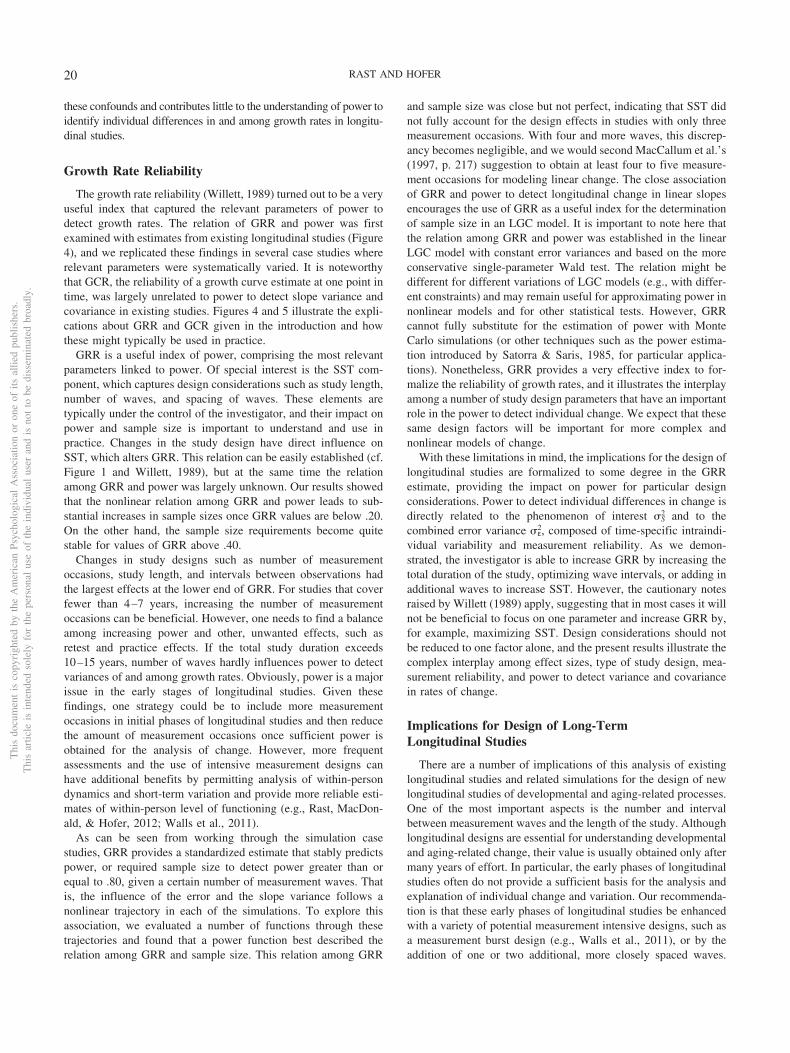
these confounds and contributes little to the understanding of power toidentify individual differences in and among growth rates in longitu-dinal studies.
Growth Rate Reliability
The growth rate reliability (Willett, 1989) turned out to be a veryuseful index that captured the relevant parameters of power todetect growth rates. The relation of GRR and power was firstexamined with estimates from existing longitudinal studies (Figure4), and we replicated these findings in several case studies whererelevant parameters were systematically varied. It is noteworthythat GCR, the reliability of a growth curve estimate at one point intime, was largely unrelated to power to detect slope variance andcovariance in existing studies. Figures 4 and 5 illustrate the expli-cations about GRR and GCR given in the introduction and howthese might typically be used in practice.
GRR is a useful index of power, comprising the most relevantparameters linked to power. Of special interest is the SST com-ponent, which captures design considerations such as study length,number of waves, and spacing of waves. These elements aretypically under the control of the investigator, and their impact onpower and sample size is important to understand and use inpractice. Changes in the study design have direct influence onSST, which alters GRR. This relation can be easily established (cf.Figure 1 and Willett, 1989), but at the same time the relationamong GRR and power was largely unknown. Our results showedthat the nonlinear relation among GRR and power leads to sub-stantial increases in sample sizes once GRR values are below .20.On the other hand, the sample size requirements become quitestable for values of GRR above .40.
Changes in study designs such as number of measurementoccasions, study length, and intervals between observations hadthe largest effects at the lower end of GRR. For studies that coverfewer than 4–7 years, increasing the number of measurementoccasions can be beneficial. However, one needs to find a balanceamong increasing power and other, unwanted effects, such asretest and practice effects. If the total study duration exceeds10–15 years, number of waves hardly influences power to detectvariances of and among growth rates. Obviously, power is a majorissue in the early stages of longitudinal studies. Given thesefindings, one strategy could be to include more measurementoccasions in initial phases of longitudinal studies and then reducethe amount of measurement occasions once sufficient power isobtained for the analysis of change. However, more frequentassessments and the use of intensive measurement designs canhave additional benefits by permitting analysis of within-persondynamics and short-term variation and provide more reliable esti-mates of within-person level of functioning (e.g., Rast, MacDon-ald, & Hofer, 2012; Walls et al., 2011).
As can be seen from working through the simulation casestudies, GRR provides a standardized estimate that stably predictspower, or required sample size to detect power greater than orequal to .80, given a certain number of measurement waves. Thatis, the influence of the error and the slope variance follows anonlinear trajectory in each of the simulations. To explore thisassociation, we evaluated a number of functions through thesetrajectories and found that a power function best described therelation among GRR and sample size. This relation among GRR
and sample size was close but not perfect, indicating that SST didnot fully account for the design effects in studies with only threemeasurement occasions. With four and more waves, this discrep-ancy becomes negligible, and we would second MacCallum et al.’s(1997, p. 217) suggestion to obtain at least four to five measure-ment occasions for modeling linear change. The close associationof GRR and power to detect longitudinal change in linear slopesencourages the use of GRR as a useful index for the determinationof sample size in an LGC model. It is important to note here thatthe relation among GRR and power was established in the linearLGC model with constant error variances and based on the moreconservative single-parameter Wald test. The relation might bedifferent for different variations of LGC models (e.g., with differ-ent constraints) and may remain useful for approximating power innonlinear models and for other statistical tests. However, GRRcannot fully substitute for the estimation of power with MonteCarlo simulations (or other techniques such as the power estima-tion introduced by Satorra & Saris, 1985, for particular applica-tions). Nonetheless, GRR provides a very effective index to for-malize the reliability of growth rates, and it illustrates the interplayamong a number of study design parameters that have an importantrole in the power to detect individual change. We expect that thesesame design factors will be important for more complex andnonlinear models of change.
With these limitations in mind, the implications for the design oflongitudinal studies are formalized to some degree in the GRRestimate, providing the impact on power for particular designconsiderations. Power to detect individual differences in change isdirectly related to the phenomenon of interest �S
2 and to thecombined error variance �ε
2, composed of time-specific intraindi-vidual variability and measurement reliability. As we demon-strated, the investigator is able to increase GRR by increasing thetotal duration of the study, optimizing wave intervals, or adding inadditional waves to increase SST. However, the cautionary notesraised by Willett (1989) apply, suggesting that in most cases it willnot be beneficial to focus on one parameter and increase GRR by,for example, maximizing SST. Design considerations should notbe reduced to one factor alone, and the present results illustrate thecomplex interplay among effect sizes, type of study design, mea-surement reliability, and power to detect variance and covariancein rates of change.
Implications for Design of Long-TermLongitudinal Studies
There are a number of implications of this analysis of existinglongitudinal studies and related simulations for the design of newlongitudinal studies of developmental and aging-related processes.One of the most important aspects is the number and intervalbetween measurement waves and the length of the study. Althoughlongitudinal designs are essential for understanding developmentaland aging-related change, their value is usually obtained only aftermany years of effort. In particular, the early phases of longitudinalstudies often do not provide a sufficient basis for the analysis andexplanation of individual change and variation. Our recommenda-tion is that these early phases of longitudinal studies be enhancedwith a variety of potential measurement intensive designs, such asa measurement burst design (e.g., Walls et al., 2011), or by theaddition of one or two additional, more closely spaced waves.
Thi
sdo
cum
ent
isco
pyri
ghte
dby
the
Am
eric
anPs
ycho
logi
cal
Ass
ocia
tion
oron
eof
itsal
lied
publ
ishe
rs.
Thi
sar
ticle
isin
tend
edso
lely
for
the
pers
onal
use
ofth
ein
divi
dual
user
and
isno
tto
bedi
ssem
inat
edbr
oadl
y.
20 RAST AND HOFER

Such study designs would refine detection of individual variationand change our understanding of intraindividual dynamics overshorter periods. Measurement-intensive designs and additionalwaves increase SST and GRR, and have a major effect on powerto detect change and covariation among rates of change if embed-ded in more typical longitudinal designs. Such innovations inmeasurement and intraindividual dynamics would carry forward inimportant ways to understand change in outcomes and processesthat may better capture the complexity of individual developmentand improve power to detect individual change and variation.
References
Baltes, P. B., & Mayer, K. U. (Eds.). (1999). The Berlin Aging Study:Aging from 70 to 100. New York, NY: Cambridge University Press.
Banks, J. A., Breeze, E., Lessof, C., & Nazroo, J. (Eds.). (2008). Living inthe 21st century: Older people in England: The 2006 English Longitu-dinal Study of Ageing (Wave 3). London, England: Institute for FiscalStudies.
Banks, J. A., Lessof, C., Nazroo, J., Rodgers, N., Stafford, M., & Steptoe,A. (Eds.). (2010). Financial circumstances, health and well-being of theolder population in England: The 2008 English Longitudinal Study ofAgeing (Wave 4). London, England: Institute for Fiscal Studies.
Barnes, G. E., Mitic, W., Leadbeater, B., & Dhami, M. K. (2009). Risk andprotective factors for adolescent substance use and mental health symp-toms. Canadian Journal of Community Mental Health, 28, 1–15.
Bauer, D. J. (2011). Evaluating individual differences in psychologicalprocesses. Current Directions in Psychological Science, 20, 115–118.doi:10.1177/0963721411402670
Berkhof, J., & Snijders, T. A. B. (2001). Variance component testing inmultilevel models. Journal of Educational and Behavioral Statistics, 26,133–152. doi:10.3102/10769986026002133
Bliese, P. D. (2000). Within-group agreement, non-independence, andreliability: Implications for data aggregation and analysis. In K. J. Klein& S. W. Kozlowski (Eds.), Multilevel theory, research, and methods inorganizations (pp. 349–381). San Francisco, CA: Jossey-Bass.
Boker, S., Neale, M., Maes, H., Wilde, M., Spiegel, M., Brick, T., . . . Fox,J. (2011). OpenMx: An open source extended structural equation mod-eling framework. Psychometrika, 76, 306–317. doi:10.1007/s11336-010-9200-6
Browne, M. W., & Cudeck, R. (1993). Alternative ways of assessing modelfit. In K. Bollen & J. Long (Eds.), Testing structural equation models(pp. 136–162). Newbury Park, CA: Sage.
Cederlöf, R., & Lorich, U. (1978). The Swedish Twin Registry. In W. E.Nance, G. Allen, & P. Parisi (Eds.), Twin research: Biology and epide-miology (Vol. 24, pp. 189–195). New York, NY: Liss.
Cohen, J. (1988). Statistical power analysis for the behavioral sciences(2nd ed.). Hillsdale, NJ: Erlbaum.
Cook, N. R., Albert, M. S., Berkman, L. F., Blazer, D., Taylor, J. O., &Hennekens, C. H. (1995). Interrelationships of peak expiratory flow ratewith physical and cognitive function in the elderly: MacArthur Founda-tion Studies of Aging. Journals of Gerontology: Series A. BiologicalSciences and Medical Sciences, 50, M317–M323. doi:10.1093/gerona/50A.6.M317
Cunningham, C. E., Boyle, M. H., Hong, S., Pettingill, P., & Bohaychuk,D. (2009). The Brief Child and Family Phone Interview (BCFPI): 1.Rationale, development, and description of a computerized children’smental health intake and outcome assessment tool. Journal of ChildPsychology and Psychiatry, 50, 416 – 423. doi:10.1111/j.1469-7610.2008.01970.x
Dixon, R. A., & de Frias, C. M. (2004). The Victoria Longitudinal Study:From characterizing cognitive aging to illustrating changes in memorycompensation. Aging, Neuropsychology, and Cognition, 11, 346–376.doi:10.1080/13825580490511161
Einfeld, S. L., Piccinin, A. M., Mackinnon, A., Hofer, S. M., Taffe, J.,Gray, K. E., . . . Tonge, B. J. (2006). Psychopathology in young peoplewith intellectual disability. Journal of the American Medical Associa-tion, 296, 1981–1989. doi:10.1001/jama.296.16.1981
Einfeld, S. L., & Tonge, B. J. (1992). Manual for the DevelopmentalBehaviour Checklist (DBC): Primary Carer Version (DBC-P). Sydney,Australia: University of New South Wales and Monash University.
Einfeld, S. L., & Tonge, B. J. (1995). The Developmental BehaviorChecklist: The development and validation of an instrument to assessbehavioral and emotional disturbance in children and adolescents withmental retardation. Journal of Autism and Developmental Disorders, 25,81–104. doi:10.1007/BF02178498
Einfeld, S. L., & Tonge, B. J. (2002). Manual for the DevelopmentalBehaviour Checklist. Melbourne, Australia: School of Psychiatry.
Ekstrom, R. B., French, J. W., Harman, H. H., & Dermen, D. (1976).Manual for kit of factor-referenced cognitive tests. Princeton, NJ: Edu-cational Testing Service.
Fears, T. R., Benichou, J., & Gail, M. H. (1996). A reminder of thefallibility of the Wald statistic. American Statistician, 50, 226–227.
Folstein, M. F., Folstein, S. E., & McHugh, P. R. (1975). “Mini-MentalState”: A practical method for grading the cognitive state of patients forthe clinician. Journal of Psychiatric Research, 12, 189 –198. doi:10.1016/0022-3956(75)90026-6
Hedeker, D., Gibbons, R. D., & Waternaux, C. (1999). Sample sizeestimation for longitudinal designs with attrition: Comparing time-related contrasts between two groups. Journal of Educational and Be-havioral Statistics, 24, 70–93.
Hertzog, C., Lindenberger, U., Ghisletta, P., & von Oertzen, T. (2006). On thepower of multivariate latent growth curve models to detect correlatedchange. Psychological Methods, 11, 244–252. doi:10.1037/1082-989X.11.3.244
Hertzog, C., von Oertzen, T., Ghisletta, P., & Lindenberger, U. (2008).Evaluating the power of latent growth curve models to detect individualdifferences in change. Structural Equation Modeling, 15, 541–563.doi:10.1080/10705510802338983
Hofer, S. M., Gray, K. M., Piccinin, A. M., Mackinnon, A., Bontempo, D. E.,Einfeld, S. L., . . . Tonge, B. J. (2009). Correlated and coupled within-personchange in emotional and behavioral disturbance in individuals with intel-lectual disability. American Journal on Intellectual and DevelopmentalDisabilities, 114, 307–321. doi:10.1352/1944-7558-114.5.307
Hofer, S. M., & Sliwinski, M. J. (2006). Design and analysis of longitu-dinal studies on aging. In K. W. Schaie & J. E. Birren (Eds.), Handbookof the psychology of aging (6th ed., pp. 15–37). San Diego, CA:Academic Press. doi:10.1016/B978-012101264-9/50005-7
Huisman, M., Poppelaars, J., van der Horst, M., Beekman, A. T. F., Brug,J., van Tilburg, T. G., & Deeg, D. J. H. (2011). Cohort profile: TheLongitudinal Aging Study Amsterdam. International Journal of Epide-miology, 40, 868–876. doi:10.1093/ije/dyq219
Hultsch, D. F., Hertzog, C., Dixon, R. A., & Small, B. J. (1998). Memorychange in the aged. Cambridge, MA: Cambridge University Press.
Hultsch, D. F., Hertzog, C., Small, B. J., & Dixon, R. A. (1999). Use it orlose it: Engaged lifestyle as a buffer of cognitive decline in aging?Psychology and Aging, 14, 245–263. doi:10.1037/0882-7974.14.2.245
Huppert, F. A., Gardener, E., & McWilliams, B. (2006). Cognitive func-tioning. In J. Banks, E. Breeze, C. Lessof, & J. Nazroo (Eds.), Retire-ment, health and relationships of the older population in England: The2004 English Longitudinal Study of Ageing (Wave 2) (pp. 217–242).London, England: Institute for Fiscal Studies.
Johansson, B., Hofer, S. M., Allaire, J. C., Maldonado-Molina, M. M.,Piccinin, A. M., Berg, S., . . . McClearn, G. E. (2004). Change incognitive capabilities in the oldest old: The effects of proximity to deathin genetically related individuals over a 6-year period. Psychology andAging, 19, 145–156. doi:10.1037/0882-7974.19.1.145
Thi
sdo
cum
ent
isco
pyri
ghte
dby
the
Am
eric
anPs
ycho
logi
cal
Ass
ocia
tion
oron
eof
itsal
lied
publ
ishe
rs.
Thi
sar
ticle
isin
tend
edso
lely
for
the
pers
onal
use
ofth
ein
divi
dual
user
and
isno
tto
bedi
ssem
inat
edbr
oadl
y.
21LONGITUDINAL STUDY DESIGN: OPTIMIZING POWER

Johansson, B., Whitfield, K., Pedersen, N. L., Hofer, S. M., Ahern, F., &McClearn, G. E. (1999). Origins of individual differences in episodicmemory in the oldest-old: A population-based study of identical andsame-sex fraternal twins aged 80 and older. Journals of Gerontology:Series B. Psychological Sciences and Social Sciences, 54, P173–P179.doi:10.1093/geronb/54B.3.P173
Juster, F. T., & Suzman, R. (1995). An overview of the Health andRetirement Study. Journal of Human Resources, 30, S7–S56. doi:10.2307/146277
Kelley, K., & Rausch, J. R. (2011). Sample size planning for longitudinalmodels: Accuracy in parameter estimation for polynomial change pa-rameters. Psychological Methods, 16, 391–405. doi:10.1037/a0023352
Kuljanin, G., Braun, M. T., & DeShon, R. P. (2011). A cautionary note onmodeling growth trends in longitudinal data. Psychological Methods, 16,249–264. doi:10.1037/a0023348
Laird, N. M., & Ware, J. H. (1982). Random-effects models for longitu-dinal data. Biometrics, 38, 963–974. doi:10.2307/2529876
Lindenberger, U., & Ghisletta, P. (2009). Cognitive and sensory declines inold age: Gauging the evidence for a common cause. Psychology andAging, 24, 1–16. doi:10.1037/a0014986
Longford, N. (1999). Standard errors in multilevel analysis. MultilevelModelling Newsletter, 11, 10–13.
MacCallum, R. C., Browne, M. W., & Sugawara, H. M. (1996). Power analysisand determination of sample size for covariance structure modeling. Psy-chological Methods, 1, 130–149. doi:10.1037/1082-989X.1.2.130
MacCallum, R. C., Kim, C., Malarkey, W. B., & Kiecolt-Glaser, J. K.(1997). Studying multivariate change using multilevel models and latentcurve models. Multivariate Behavioral Research, 32, 215–253. doi:10.1207/s15327906mbr3203_1
Maxwell, S. E. (1998). Longitudinal designs in randomized group comparisons:When will intermediate observations increase statistical power? Psycholog-ical Methods, 3, 275–290. doi:10.1037/1082-989X.3.3.275
Maxwell, S. E., Kelley, K., & Rausch, J. R. (2008). Sample size planningfor statistical power and accuracy in parameter estimation. AnnualReview of Psychology, 59, 537–563. doi:10.1146/annurev.psych.59.103006.093735
McArdle, J. J. (1988). Dynamic but structural equation modeling of re-peated measures data. In J. R. Nesselroade & R. B. Cattell (Eds.),Handbook of multivariate experimental psychology (2nd ed., pp. 561–614). New York, NY: Plenum Press.
McArdle, J. J., & Epstein, D. (1987). Latent growth curves within devel-opmental structural equation models. Child Development, 58, 110–133.doi:10.2307/1130295
McClearn, G. E., Johansson, B., Berg, S., Pedersen, N. L., Ahern, F.,Petrill, S. A., & Plomin, R. (1997). Substantial genetic influence oncognitive abilities in twins 80 or more years old. Science, 276, 1560–1563. doi:10.1126/science.276.5318.1560
Muthén, B. O., & Curran, P. J. (1997). General longitudinal modeling ofindividual differences in experimental designs: A latent variable frame-work for analysis and power estimation. Psychological Methods, 2,371–402. doi:10.1037/1082-989X.2.4.371
Muthén, L. K., & Muthén, B. O. (2010). Mplus user’s guide (6th ed.). LosAngeles, CA: Muthén & Muthén.
Paxton, P., Curran, P. J., Bollen, K. A., Kirby, J., & Chen, F. (2001). MonteCarlo experiments: Design and implementation. Structural EquationModeling, 8, 287–312. doi:10.1207/S15328007SEM0802_7
Piccinin, A. M., & Rabbitt, P. (1999). Contribution of cognitive abilities toperformance and improvement on a substitution coding task. Psychologyand Aging, 14, 539–551. doi:10.1037/0882-7974.14.4.539
Pinheiro, J. C., & Bates, D. M. (2000). Mixed-effects models in S andS-PLUS. New York, NY: Springer. doi:10.1007/978-1-4419-0318-1
Radloff, L. S. (1977). The CES-D scale: A self-report depression scale forresearch in the general population. Applied Psychological Measurement,1, 385–401. doi:10.1177/014662167700100306
Rast, P., MacDonald, S. W. S., & Hofer, S. M. (2012). Intensive measure-ment designs for research on aging. GeroPsych, 25, 45–55. doi:10.1024/1662-9647/a000054
Raudenbush, S. W., & Bryk, A. S. (2002). Hierarchical linear models:Applications and data analysis methods (2nd ed., Vol. 1). ThousandOaks, CA: Sage.
Raven, J. C., Court, J. H., & Raven, J. (1995). Manual for Raven’sProgressive Matrices and Vocabulary Scales. Oxford, England: OxfordPsychologist Press.
R Development Core Team. (2012). R: A language and environment forstatistical computing [Computer software manual]. Vienna, Austria: RFoundation for Statistical Computing. Retrieved from http://www.r-project.org
Roth, M., Tym, E., Mountjoy, C. Q., Huppert, F. A., Hendrie, H., Verma,S., & Goddard, R. (1986). CAMDEX. A standardised instrument for thediagnosis of mental disorder in the elderly with special reference to theearly detection of dementia. British Journal of Psychiatry, 149, 698–709. doi:10.1192/bjp.149.6.698
Satorra, A., & Saris, W. (1985). Power of the likelihood ratio test incovariance structure analysis. Psychometrika, 50, 83–90. doi:10.1007/BF02294150
Savage, R. D. (1984). Alphabet Coding Task–15. Unpublished manuscript,Murdoch University, Perth, Australia.
Schaie, K. W. (1985). Manual for the Schaie–Thurstone Adult Mental AbilitiesTest (STAMAT). Palo Alto, CA: Consulting Psychologists Press.
Schaie, K. W., & Hofer, S. M. (2001). Longitudinal studies in aging research. InJ. E. Birren & K. W. Schaie (Eds.), Handbook of the psychology of aging(5th ed., pp. 53–77). San Diego, CA: Academic Press.
Stoel, R. D., & van den Wittenboer, G. (2003). Time dependence of growthparameters in latent growth curve models with time invariant covariates.Methods of Psychological Research, 8, 21–41.
Thurstone, L. L., & Thurstone, T. G. (1949). Examiner manual for the SRAPrimary Mental Abilities Test. Chicago, IL: Science Research.
Tisak, J., & Meredith, W. (1990). Descriptive and associative developmen-tal models. In A. von Eye (Ed.), Statistical methods in longitudinalresearch (Vol. 2, pp. 387–406). New York, NY: Academic Press.
Venables, W. N., & Ripley, B. D. (2002). Modern applied statistics with S(4th ed.). New York, NY: Springer.
von Oertzen, T., Ghisletta, P., & Lindenberger, U. (2010). Simulatingstatistical power in latent growth curve modeling: A strategy for eval-uating age-based changes in cognitive resources. In M. W. Crocker & J.Siekmann (Eds.), Resource-adaptive cognitive processes (pp. 95–117).Berlin, Germany: Springer-Verlag. doi:10.1007/978-3-540-89408-7_6
Walls, T. A., Barta, W. D., Stawski, R. S., Collyer, C., & Hofer, S. M.(2011). Time-scale-dependent longitudinal designs. In B. Laursen, T. D.Little, & N. Card (Eds.), Handbook of developmental research methods(pp. 46–64). New York, NY: Guilford Press.
Wechsler, D. (1991). Manual for the Wechsler Adult Intelligence Scale–Revised. New York, NY: Psychological Corporation.
Willett, J. B. (1989). Some results on reliability for the longitudinalmeasurement of change: Implications for the design of studies on indi-vidual growth. Educational and Psychological Measurement, 49, 587–602. doi:10.1177/001316448904900309
Zelinski, E. M., & Burnright, K. P. (1997). Sixteen-year longitudinal andtime lag changes in memory and cognition in older adults. Psychologyand Aging, 12, 503–513. doi:10.1037/0882-7974.12.3.503
Received June 11, 2012Revision received July 27, 2013
Accepted August 7, 2013 �
Thi
sdo
cum
ent
isco
pyri
ghte
dby
the
Am
eric
anPs
ycho
logi
cal
Ass
ocia
tion
oron
eof
itsal
lied
publ
ishe
rs.
Thi
sar
ticle
isin
tend
edso
lely
for
the
pers
onal
use
ofth
ein
divi
dual
user
and
isno
tto
bedi
ssem
inat
edbr
oadl
y.
22 RAST AND HOFER