i wmiiii*!—WB—■—n —TT""""1" .mmm&wum-

AD-769 221

LONGITUDINAL MANPOWER PLANNING MODELS

Richard C. Grinold, et al

California University

Prepared for:

Office of Naval Research

August 1973

DISTRIBUTED BY:

KJÜ1 National Technical Information Service U. S. DEPARTMENT OF COMMERCE 5285 Port Royal Road, Springfield Va. 22151

Unc1 ssifled Socunty Cl.issificntion /?/)7C9^4/

DOCUMENT CONTROL DATA -R&D St-i nrffi ctnuitfcutton uf fitly, hinly ol tthBlfiWt tuitl ittdvtttit^ •umululhtn mif»! hr vnu-rvü wlwn thr itvvtitU repttrt is cluhtiifivit)

O^IOIN* TING ACTIVITV fCorfturmf itttthur)

University of California, Berkeley

til. Ht POXT SECUniTV Cl ASSIFIC < 1 IOM

Unclassified 2li GROUP

i RfPORT ntLF

LONGITUDINAL MANPOWER PLANNING MODELS

4 ocscRiPTivic HOTES (Type ol report »nd.lnctusive date*)

Research Report ; «UTHORISI (First name, middle initial, Imm nome)

Richard C. Grlnold, Kneale T. Marshall and Robert M. Oliver

6 REPORT OA TE

August 1973 »a. CONTRACT OR GRANT NO.

N00014-69-A-0200-1055 b. PROJEC T NO.

NR 047 120

7«. TOTAL NO. OF PAGES

gg J£ lb. NO. OF REFS

9». ORIGINATOR'S REPORT NUMBER(S)

ORC 73-15

9b. OTHER RFPORT NOISI (Any other numbers that may be amslgned this repotl)

10 DISTRI BUTION STATEMENT

This document has been approved for public release and sale; its distribution is unlimited.

II i^-^LiMENTARY NOTES

None

•1 ---JSTPACT

12. SPONSORING MILITARY ACTIVITY

Office of Naval Research Department of the Navy Arlington, Virginia 22217

..,

SEE ABSTRACT.

*'"O6M£SL\ TECHNICAL NATIONAL it V4CE iNfORMA^VT

SPW1'"

Jj£

S/N 0101-807-6RIt Unclassified Socufily Classification

A-3140-i

«■■■^HHiVM^^VI^H^HMWBH wimumwium^^^BKmwi

Unclassified Security ClttRsifu'ation

KEY WORDS

HOLt IKT

Manpower Planning

Cohort Model

Linear Programming

Infinite Programs

Manpower Data

DD .F.r.,1473 'BACK) 11 ,• I - ro ; •,. . i

Ik 1 Unclassified Security Classification

1

LONGITUDINAL MANPOWER PLANNING MODELS

by

Richard C. Grinold, Kneale T. Marshall and Robert M. Oliver Operations Research Center

University of California, Berkeley

) (i

,' NOV 1% 1373 ; M

i

E

AUGUST 1973 ORC 73-15

This research has been supported by the Office of Naval Research under Contract N00014-69-A-0200-1055 with the University of Caa.ifornia. Reproduction in whole or in part is permitted for any purpose of the United States Government.

ri

I

ABSTRACT

Several manpower planning models are presented that exploit the longitudinal stability of manpower cohorts. The manpower planning process is described along with the problem of identi- fying and obtaining various types of longitudinal data. An infinite horizon linear program for calculating minimum cost manpower input plans is found to have a straightforward solution in a great many cases and to yield an easily implemented approxi- mation technique in other cases.

Mi

./

1. INTRODUCTION

This paper formulates manpower planning models for a system consisting of

many skill categories; the particular application is to the enlisted force in

the U.S. Navy. Interactive computer models of these theoretical formulations

have been developed and implemented to aid decision-makers who wish to test

the effects of alternative manpower policies on staffing requirements and fu-

ture manpower budgets. These interactive manpower planning models have a

variety of uses, to:

(1) predict the manpower requirements that will be fulfilled by the

current stock of manpower.

(2) calculate unfulfilled requirements and the new Inputs necessary to

meet them.

(3) identify bottlenecks In the manpower planning process.

(4) assist in preparation of future manpower budgets.

(5) simulate the effects of manpower policy changes on future manpower

needs.

(6) relate alternate personnel retention and performance assumptions to

the need for future inputs.

(7) calculate minimum co&'c input schedules when lower bounds on require-

ments are given.

Details of the interactive positions of the models are not included here since

they are to a large extent dependent on the particular hardware/software com-

bination used. Rather we emphasize the underlying mathematical structure.

Individuals in any skill category can be Identified by several character-

istics: examples are; rank, salary, number of years of experience in the skill

category, length of service in the Navy, and personal attributes such as age

and measures of performance. The models presen*- d in this paper are designed

2

to assist In preparing manpower budgets and meeting aggregate strength require-

ments. For these purposes we have chosen to Identify Individuals In the enlisted

force according to skill category and length of service (LOS) In the Navy.

Section 2 of the paper describes the underlying manpower flow models.

The models are based on the assumption of longitudinal stability In the service

lifetimes of different manpower cohorts. We show that the accession schedule

that exactly meets requirements Is found by solving a set of lower triangular

system of linear equations. Section 3 relates several methods of describing

the longitudinal behavior of manpower cohorts and shows how the flow model's

parameters can be estimated from existing Navy data. In Section 4 we present

an ii finite horizon linear program for the calculation of future manpower in-

puts and strength levels with the objective of minimizing discounted costs.

We derive readily verifiable conditions on the inputs to the infinite horizon

problem that guarantee that the equality solution, described in Section 2, will

be optimal. In cases where the equality solution is not optimal we describe

a finite linear program that will approximate solutlois of the infinite horizon

program.

The models presented in this paper examine the relationships between three

factors: (1) the current manpower situation as described by the LOS distribu-

tions of different skill ratings, (li) the survivor fractions that will deter-

mine the lorgitudlnal behavior of manpower cohorts, and (ill) the manpower

requirements for future times. The size of our models and the type of calcu-

lations performed allow policy makers to quickly analyze the impact of various

assumptions and policies.

-

2. THE UNDERLYING COHORT FLOW MODELS

We consider an organization which is divided into many skill categories

vlare movement between categories typically involvas retraining of the indi-

vidual. In this paper we consider each skill category separately; a subsequent

paper, will discuss transfers and other interactions between skill cate-

gories.

We idealize the evolution of the skill category by analyzing its changes

at discrete points in time (i » ... -2,-1,0,1,2, ...) . We say that period

i is the interval between times (1 - 1) and i ; it is a future period if

i > 1 , a past period if i < 0 , and the current period if i = 1 . In period

i a number of people x. enter the skill category; that group is called

cohort i and x. is the number of accessions in cohort i . Let a . be

the fraction of the cohort entering in period 1 which is still present and

available to meet requirements at time 1 + J (j ü 0) . Let z. be the re-

quirement in the skill category at time k and let (m + I) be the maximum

number of periods an individual is allowed to stay in the system. Thus

o.. = 0 if 1 > m . For some future time k we have ij J

(1) \ " Vk,0 + VlVl,l + ''' + VmVm.m '

Equation (1) simply says that the requirement at time k is made u.) of frac-

tions of cohorts which survive from earlier periods. Thus it is natural to

call the n^'s the suwivoi' fvaotions for the cohort which enters at time i .

At time 0 , the history of past accessions is given by the vector

(x ,xn , ..., x ..x ,.x.) . The current inventory of people Is given by —m A-m —/ -i u

XA01« ri + x,a+...+x a , and contains the remaining fractions or

0 0,0 -1 —1,1 -m -m,m

past inputs. This quantity is called the current legacy, say y. . In future

period k the legacy y, from past inputs up to and including period 0 will

be

: *&•■

(2)

y, ■ x_a- ,+x,a,,1, + ...+x1 a ,._» if k<ni, 7k 0 0,k -1 -l,k+l k-m, -m.k+m -

»0 if k > m .

Suppose we have a planning horizon of T periods with requirements

z-,2», ... 2_ . From equations (1) and (2) we see that future cohort sizes

must satisfy

ai.oxl = Zl - yl

al.lXl + a2.0x2 Z2-y2

(3) • • • • • •

alfT-lXl + 02.T-2X2 + '•• + aT.0XT = ZT " yT

Here we have assumed

Al: requirements are met exactly.

Under Al It Is quite possible that for a given set of z.'s , y,'s and

a, 's some x. could be negative. Such a result would say that in order

to exactly meet requirements In all periods 1,2, ..., T it will be necessary

to remove people from the skill category in period k . In practice, this

might be accomplished through retraining.

This section concentrates on the equality solution for several reasons.

First, It is misleading to state the problem as if the accessions (the x, )

are the only variables which the decision-maker can influence. The legacies

(y,) , requirements (z. ) and to some extent the survivor fractions (a..)

Recall that «11 = 0 if j > m .

can all be changed or explicitly influenced by manpower policies. Second,

plans that are eventually recommended will probably conform to the equality

constraints since budget restrictions do not generally allow for slack in the

system. Third, we intend to use the models in this section to test the ef-

fects of alternate policies on several objectives: (1) the departure of

realistic requirements from ideal requirements, (2) the smoothing of stocks

and accessions, (3) the Impact of policy changes on personnel and finally

(4) the retraining costs associated with switching personnel from one spe-

cialty to another. In Section 4 we shall drop Al and treat the net require-

ments as lower bounds and look for cost minimizing accession schedules.

In the remainder of this paper we make an important second assumption

A2: the survivor fractions a are stationary from period to period, l»j

That is, a = a , independent of i and independent of x, . "'•» J J i

Under assumption A2 equation (3) to simplify to

Vi = zl - yl

(4) Vl + V2 ^ Z2 - y2

aT-lXl + V2X2 + ••' + VT = ZT - yT

In these equations the legacies are given by

Vo + V-i + + a x, m 1-m

(5) Yo = Vo + V-i + + a x m 2-m

yT - aTx0 + ... + a^

Equation (4) can be used In a number of ways. We have mentioned already

that given the requirements, legacies and survivor fractions, (4) can be used

to calculate new cohort Input requirements for each period of the planning

horizon T . Alternatively, given planneo Inputs over the next T periods

the z.'s can be considered as the result of these Inputs. Also, given re-

quirements and planned Inputs, the legacies which satisfy equation (4) can

be determined. These possibilities will be discussed further tu the section

on Interactive programming.

To this point we have motivated equations (4) and (5) by considering z.

and y. as stocks of people and x as a flow of people per year. It is not

necessary to define a , x , y , and z In that manner. We could also speak

of stocks and flows of money or effective personnel or use another unit of

time. For example If c. Is the cost associated with an individual in the

j year of service, the total cost In year i will be

, (6) CrtO-x. + c,a,x. i ... + c a x. v ' 0 0 111 1-1 m m 1-m

The cost legacy, that will be Incurred in future period 1 due to current,

period 0 , manpower legacies is

(7) c.a.xn + c-.-a.-.x, ... + c a x. ' 1 i 0 1+1 1+1 1 mm i-m

The use of equations (4) and (5) depends on the availability of data to

estimate the various parameters. The next section examines several possible

data configurations and presents some actual examples of U.S. Navy enlisted

force data.

3. DATA

To employ nhe cohort model described in Section 2, it is necessary to

obtain information about past accessions x. and some knowledge about past

survivor fractions a . Typically, data which is available in most organi-

zations is of the cross-sectional type. Thus we may know the number currently

in a given skill category and the length of time each person has been in the

category. In the case of the U.S. Navy enlisted force this type of cross-

sectional information is available for a number of past planning periods.

Data on the past Inputs and the survivor fractions are not available, and

so we must either eliminate these from our equations or find methods of de-

termining them from available data.

We shall demonstrate below how estimates of the survivor fractions and

past skill category accessions can be obtained from several different config-

urations, and present an example using U.S. Navy data. The reader should,

however, not focus too strongly on the problem of estimating survivor frac-

tions from historical data. Survivor fractions realized by past cohorts are

the result of former manpower policies, and the cohort's behavioral charac-

teristics. In the context of the U.S. Navy these data are influenced by early

out policies, retraining and transfer decisions, changes in the length of

tours, the mixture of regular and reserve forces, and the fraction of draft

motivated accessions. Simple projections using historical estimates of sur-

vivor fractions will, at best, show the results of continuing past manpower

policies. The specification of future survivor fractions is, to a great ex-

tent, the specification of future manpower policy.

Despite this warning on the use of historical estimates, we shall now

show how these estimates can be made with several different data configura-

tions. In the first case we assume that past accession levels x. for i <^ ü ,

are known as well as part stocks z . Equation (1) of Section 1, combined

with assumption A2 can be written

W «j " «j^O + xj-l0l + Xj-2a2 "• + xj-mam *

If z. Is known for j ■ 0,-1, ..., -m and x. for j = 0,-1, ..., -2m ,

then system (1) represents m 4- 1 equations In the m + 1 unknowns

's ,a., ..., a . However, it Is highly unlikely that data on skill category

inputs will be maintained at the precise degree of aggregation called for by

the model over the past 2m periods. We might find the aggregate Input Into

several skill levels, or a change in manpower accounting methods in the past

2m periods. Thus, in general, it is necessary to estimate the survivor frac-

tions without knowledge of past accessions.

We are now left with the task of using the models described in Section 2

when past accessions are not known and cross-sectional data is available. We

define a., to be the number of people in year 1 with J years of service.

From the cohort assumption A2,

(2) n^ - x^oj .

An Individual has j years of service if his length of service (LOS) lies in

the Interval [J,j + 1) . It does not follow that an Individual with I.0S

equal to j has been in a skill category for J years. It is possible to

be unrated for several years, and it is possible to be transferred between

skill categories. In many of the critical highly trained ratings, however,

the LOS and time in skill category coincide.

Note that formula (2) allows one to calculate the legacy without knowledge

of the past accession levels. Given tin current longitudinal data nn. and

the survivor fractions i:-. that will obtain in future periods, formula (2)

can be used to calculate the past acce^ion levels that would be consistent

with both current LOS data and the assumption that the survivor fractions ctj

applied in past periods. These accession levels can then be used In equation

(5) of Section 2 to calculate the legacy.

It remains to find some method of estimating the survivor fractions and

of relating them to other measures of longitudinal stability namely: the con-

tinuation rate ß. , and the age fraction y.. . These measures will be de-

fined, and then related to the survivor fractions a. , and cross-sectional

data n., .

The continuation rate 3. is defined as

n. .

:, Vi.j-i

It is most convenient to interpret 3, as the fraction of those with j - 1

years of service in year i - 1 , that remain (continue) in year i . It is

possible, although this effect is not explicitly considered in our model, to

enter a skill category with more thn one year of se-vice. Therefore histori-

cal estimates of ß, from reliable data can yield numbers that are greater

than one. The notation has anticipated the result that ß. is independent

of i due to assumption A2. From (2), we have

Xl-iai 0l1 (A) ß. =- i-J-i "T2-- j-1,2. ...,m.

3 xi-l-(j-l)aj-l aj-l

The value of ß0 " 1 is assumed. Thus we can calculate ß from a using u

(4) and the reverse calculation is simply:

"J = "° k 6J (5) a = a £ ß j = 1,2, ... m .

The age fraation y is the fraction of people in year i that have j

years of service. It follows thnL

10

Y -^

m where z 4 " 1 n4i ' w^en assumption A3 holds, theu

1 J-0 1J

Y .^i

To be a useful measure of longitudinal stability, the y,. should be sta-

tionary, i.e. independent of i . However, stationary age fractions are in

general incompatible with assumption A2. In particular, if A2 holds and y..

is independent of i , then one can easily determine that the system must be

growing at a constant rate (9 - 1) with x. e 9 x- , z. => 0 20 , and

Y ii i

6 z0

We have seen that the survivor fractions a , and continuation rates $ ,

are useful measures of longitudinal cohort stability, while the age fraction

y.. does not isolate the effects of varying past levels of accessions from

the behavior patterns of the cohorts. We conclude this discussion with a

formula that shows how the quantities a , ß , y are calculated from the

cross-sectional data. Since the a and ß are essentially flow rates, at

least two years of cross-sectional data are necessary to determine their values.

ni^.a Vii j ni-l,J-l zi-lYi-l,j-l

(6)

o o . "ij ••• ni2'nll

J Vi.j-i '•• ni-i,i'ni-i,o Oo *

In what follows we shall demonstrate how these concepts can be applied to

some actual data.

11

The flow models described in Section 1 were designed to assist in man-

power planning for the U.S. Navy's enlisted ranks. That force comprises

approximately 550,000 people in nine ranks and c'O skill categories which

are commonly called ratings.

Tables 1 and 2 contain the length of service distributions of five ratings.

If we take June 30, 1972 to be time 0 , then Table 1 gives the values of

n . . and Table 2 the values of nrt . . The particular data presented in

Tables 1 and 2 was abstracted from Rating Career Factor reports prepared by

the Personnel System Research Department of the Naval Personnel Training and

Research Laboratory, San Diego.

The Rating Career Factor reports contain the tail of the age fraction as

well as the total Inventory z in each rank. Let T , be the fraction in

period i , that have completed j or more periods of service. Clearly

ri,j ' Yl,j + Yi.j+1 •,, +Yi,in

and

Y = r - r Yij l.j i,j+l

Thus to find n.. we must calculate

nij " 2i(ri,j " ri,j+l) *

For the Boatswain's Mate rating we have

n0.5 = z-l(r-1.5 " r-l,6)

= (10973)(5.97 - 56.2) = 384 .

The original source of this data is the enlisted personnel master tape,

that is maintained by the Management Information Division of the Bureau of

Naval Personnel (Pers N). The data kept by Pers N is used on a daily basis

for current management of the Navy; it is a necessity of the cross-sectional

12

TABLE 1

LENGTH OF SERVICE DISTRIBUTIONS AS OF 6/30/71

Length of Service

0

1

2

3

4

5

6

7

8

9

10

11

12

13

14

15

16

17

18

19

20

21

22

23

24

25

26

27

28

29

BM QM Ratings

ET CS ET

225 1186 5044 1435 1488 1547 1078 3848 1372 1926 1513 911 3544 1173 2156 382 82 2305 357 198 438 141 1762 503 285 449 87 ' 762 493 340 438 125 653 399 318 449 141 544 325 285 561 152 479 378 285 516 130 436 315 340 449 168 414 284 274 404 125 371 231 329 348 130 349 231 351 326 130 262 273 351 471 168 197 451 548 516 168 218 545 559 236 103 131 294 209 427 93 110 503 307 483 103 88 420 220 124 28 44 116 56 57 17 23 32 23

102 17 23 43 23 158 28 44 64 23 102 12 23 32 1 124 17 23 64 23 79 17 23 32 23 91 17 23 32 12

102 17 23 53 1 79 17 1 32 12 35 6 1 11 1

TABLE 2

LENGTH OF SERVICE D1FTRIBUTIONS AS OF 6/30/72

13

Length of Service

0

1

2

3

A

5

6

7

8

9

10

11

12

13

14

15

16

17

18

19

20

21

22

23

24

25

26

27

28

29

BM QM Ratings

ET CS ET

166 1317 357 Ü 1649 2501

769 596 3578 830 961

2832 1050 3578 1489 2026

319 107 2996 331 286

341 62 2091 321 170

385 132 1121 470 254

418 87 647 480 317

418 117 518 361 275

418 122 454 301 254

484 137 432 351 254

495 127 410 311 317

429 157 389 291 254

395 117 367 231 317

330 132 324 231 339

219 127 238 261 349

462 167 195 441 539

495 167 216 530 560

231 97 130 291 201

297 62 87 311 170

253 56 23 191 3b

78 16 23 71 33

45 11 23 21 12

67 16 23 31 22

122 21 44 41 12

78 11 23 31 12

100 6 23 41 12

67 16 23 21 22

78 11 1 41 1

89 21 23 41 12

23 6 1 11 1

1A

type. That Is, on any given day, their data file gives a current listing of

Navy Personnel. We obtained values of n . . from report E1S-9H, Pers A12,

Bureau of Naval Personnel, dated 9/30/71. These values conformed closely to

the n . . calculated from the age tails. From Tables 1 and 2, we see that -1| J

on June 30, 1971 there were 1513 people in the category "Boatswain's Mate" in

the Navy with between 2 and 3 years of service. Similarly there were 371

"Electronics Technicians" with more than 11 and not more than 12 years of

service.

Using this data and formula (6), we can calculate a point estimate of

the continuation rates 0. . For example for Boatswain's Mates.

4 n.jj 382

on

, rX2_ 2832 „ 8 32 n . ' 1547 1-83 *

In this case, we see that the continuation rate exceeds 1. This is due to a

large number of inputs into BM rating with two years of unrated service. The

continuation rates and survivor fraction calculated for the skill categories

BM and ET are presented in Tables 3.

In the critical skill, ET, the continuation rate? are less than 1 and

survivor fractions decrease. This follows from the Navy's practice of training

ET's from recruits with a zero LOS. The BM rating draws its input from the

unrated enlisted ranks, and generally with an LOS equal to 2. The BM survivor

fractions can be modified by dividing them by a. = 6.28 . The modification

allows us to Interpret x as the number of accessions at time 1 that even-

tually enter the BM skill category, and ax. as the number in the BM skill

category in period i + j .

15

LOS

0

1

2

3

4

5

6

7

8

9

10

11

12

13

14

15

16

17

18

19

20

21

22

23

24

TABLE 3

CONTINUATION RATES

BM ET

1 1

3.43 0.71

1.83 0.93

0.21 0.85

0.89 0.91

0.88 0.64

0.33 0.85

0.95 0.79

0.93 0.83

0.86 0.90

0.96 0.94

0.96 0.94

0.98 0.99

0.95 0.93

0.98 0.91

0.98 0.99

0.96 0.99

0.98 0.99

0.70 0.79

0.52 0.25

0.62 0.50

0.78 0.99

0.65 0.99

0.77 0.99

0.76 0.99

SURVIVOR FRACTIONS

BM ET

1 1

3.43 0.71

6.28 0.66

1.32 0.56

1.18 0.51

1.04 0.32

0.97 0.27

0.92 0.22

0.85 0.18

0.74 0.16

0.70 0.15

0.68 0.14

0.66 0.14

0.63 0.13

0.62 0.12

0.60 0.12

0.57 0.12

0.57 0.12

0.39 0.09

0.20 0.02

0.12 0.01

0.10 0.01

0.07 0.01

0.05 0.01

0.04 0.01

16

4. MINIMIZING ACCESSION COSTS

The accession schedule that meets future manpower requirements z exactly

is lound by solving the equations

Vo = zi - yi

Vl + a0X2 ^ Z2 - y2

(1) a^ .x. + a _x- + ... + anx - z - y m-1 1 m2 2 0 m m ym

a x, + a , x- + ... + a, x + aAx ,, = z ., m 1 m-1 2 1 m 0 nrfl m+l

a x- + ... + a-x + a-x_., + artx_. . " z_. . m 2 2ml m+l 0 nri-2 m+2

In this section we shall relax the assumption that future manpower require-

ments are satisfied exactly. Instead we shall treat the variables z AS

lower bounds on the manpower level at time t . Moreover, we shall restrict

the accessions x to be nonnegative. Thus the equalities in (1) will be

replaced by inequalities (>) . This leaves us with an infinite system of

linear inequalities that will, in general, have a large number of possible

solutions. To obtain a single accession schedule in this case we can specify

a performance criterion and then select the accession schedule that optimizes

that criterion.

In the analysis that follows we assume that the performance criterion is

to minimize the present worth of all future accession costs. This objective

ia obtained by discounting future costs to today's dollars and then summing

ove: all future periods.. We obtain the extremely simple and useful result

17

that the optimal accession schedule is Independent or the costs. In addition,

we will show that there are many conditions of practical interest when the

equality solution discussed in earlier sections is indeed an optimal solution

to the infinite-horizon program. Finally, we will discuss several practical

methods by which the infinite program can be truncated and approximated by a

finite program with T rather than an infinite number of periods. The method

of truncation that should be used depends on the conditions the user wishes to

assume for planning periods in the distant future.

The Infinite Horizon Program

Thera are several approaches to the solution of (1) when the restriction

of exactly meeting the mar ^. rer requirements is relaxed. In describing a cost

minimization model in which the manpower requirements are considered to be

lower bounds we assume that manpower requirements can in fact be modelled by

such inequality restrictions.

The problem is to choose the nonnegative vector (xj.x«, ...) that

satisfies

(2)

Vl ^ zl " yl

Vl + V2 - Z2 - y2

Vl + V2 + a0X3 - Z3 - y3

x > 0

Note that it is possible to consider x as the number of accessions above

some minimal level. Then z should be interpreted as the requirements left

unsatisfied by the minimal accession schedule.

Let c, for k = 0,1,2, .... m be the cost of training and support of

&

18

an Individual In the k year of service. The discounted cost of an accession

Is thus

m "> m (3) c - I (V )6J - a0c0 + o c 6 + a ^6^ + ... + a^ö"1

j«0 J J

where 6 is a discount factor less than one. The total discounted cost of

an accession schedule (x..,x_, ...,) is therefore

(A) J cx.,6"1 « ex. + öcx- + S ex- + ...

■

j-l *

Since an accession in any period j costs ö c t it is evident that the

value of c will not affect the optimal eotution. In fact, we can, without

any loss in generality, use

* „ J-l I x S^ » x + 6x9 + 6 x_ + ... j-l -' X * J

as the objective to be minimized subject to the constraints in (2).

The Dual Progra'a and Optimality Conditions

The dual of the infinite linear program in (5) and (2) Is to find non-

negatlvt variables u ,u?, ... which

(6) Maximize u^Zj^ - y^ + u2(z2 - y ) +

subject to the inequality constraints

UjO- + u-a + u.a + ... < 1

(7) u2a0 + u-a + ... _< 6 "j. i 0

2 u-a + ... < 6

19

A feasible solution of the dual problem always exists and is given by

u = vi6 , where y = 1/j ^ a ö-5 J . This solution is strictly positive VJ-O 3 /

and satisfies each dual constraint as an equality.

The main results of linear programming do not carry over to infinite

linear programs; the strong duality theorem can fall, [1], and in some cases

even the weak duality thenem and the related sufficiency condition (comple-

mentary slackness) can fail, [2]. Fortunately, our problem has a great deal

of special structure and under two reasonable assumptions we shall establish

a useful lower bound on the optimal value of the infinite problem and deter-

mine that the solution of (1) is optimal if it is nonnegative, i.e. feasible.

The first assumption is that »n > 0 and that «^ ^ 0 for all j .

th m

The second assumption is on the m order difference equation ^ ax . =• z , j=0 J ^ t

with initial conditions given by (xQ,x,, ..., x, ) . It is obvious from

equation (5) in Section 2 that the Initial conditions are also specified by

the legacy y, ,y,,, ..., y , and that the unique solution of this difference

equation is simply the solution of (1) in this section. The difference equa-

tion is called asymptotically stable if all the complex roots of its charac-

m . teristic polynomial J a.w ^ , have absolute value strictly less than one.

In particular, the condition is satisfied if: 1 > a. > a... and o. . > a. > «... j J"'"! l—i 1 i+1

■■

for some 1 , and appears to be satisfied by other survivor fraction data that

we have encountered to date. In, [3], Chapter 10 it is demonstrated that

asymptotic stability implies that for any initial conditions and any bounded

z the solution of the difference equation will be bounded. Let x be the t t

unique, bounded solution of (1). From our two assumptions it follows that

x = Max (0,x ) is a bounded and feasible solution for the constraints (2).

To establish optlmality conditions it is useful to examine the T period

approximations of the infinite problem. The T period problem is

20

T Minimize I fr5'1*.

t-1 (8) Su bject to ^o «jx^j > «t - yt

x > 0 for t - 1,2, ..., T

Notice that any solution of the infinite problem will have Its first T com-

ponents (x-.x-, ..., x ) feasible for the T period approximation. Moreover,

the solution u - yfi ~ for t - 1,2 T will be feasible for the dual

of problem (8). Thus by the weak duality theorem for problem (8), we have

t-i c t-i z z

for all T and any solution of the Infinite problem. This gives us a lower

as

bound J y6 ~ (z - y ) on the optimal value of the infinite problem.

t-1

Finally, since 6 < 1 , and x is bounded it is possible to show that

00 CO

^6 x - ^ yfi (z - y ) . Thus the possibly infeasible solution x t"l t"l

achieves the lower bound. It follows that x is optimal If it Is fearible.

I.e. if each element of x la nonnegative.

In summary the result of tnis section is th'c under the hypothesis of

asymptotic stability, boundedness of the requirements sequence z , and

nonnegatlvity of t'ae survivor fractions, the equality solution x la optimal

If it Is nonnegative.

Optimality of Equality Solution

Intuition suggests the equality solution of (2) will often be an optimal

solution of the infinite horizon planning problem posed In (5). Identification

of the conditions which must exist for the equality solution to be nonnegative

21

and thus optimal gives considerable insight into the structure of the problem.

These conditions place bounds on the magnitude of allowable changes in future

manpower requirements. Moreover, optimality of the equality solution gives us

an analytic expression for total system cost as a function of the continuation

rates, net requirements, and costs.

To begin the analysis of this section we look for solution of a reduced

system of linear equations

x. =1

61x1 + x2 = ^

ß1ß2x1 + Plx2 + X3 - ^2

3l02ß3Xl + ßlß2X2 + ßlX3 + X4 = ♦iVa

which is equivalent to normalizing the equality system in (1) by the constant

Zl-yl In (9) (|), is defined to be the ratio of successive net require- ao 3

ments, i.e. z.+1 - y^+i/z^ ~ y^ • Alternatively, one can view (9) as the

equality system in (2) with a0 « 1 , ß.fä- ... jJ. ■ a. , z, - y. ■ 1 and

(z,+1 - yj+1) = <t,1|j)? • • • "frj • In either case, multiplicatioi of a solution

vector x = (x^x^, ...) of (9) by z.. - y-i/a« yields the equality solution

of (1). It should be not 2d by the reader that just as the continuation rates

ß^ß«, ... 3 measure the period to period increases or decreases in the

fraction surviving an additional period, the growth rates «J»,,«^, ... <(».

measure the period to period ■'ncreases or decreases in the net requirements

that must be met by new accessions.

With this definition of terms it is tempting to believe that so long as

—■MM—«»H»:^^- .,

22

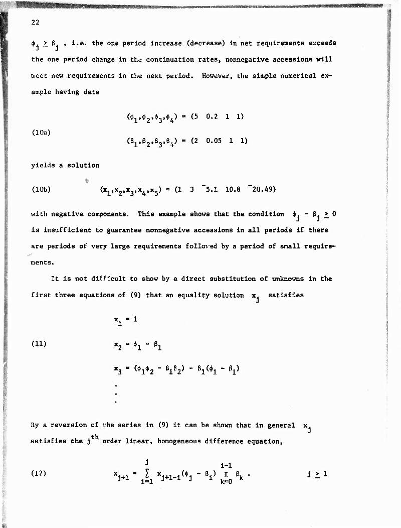
♦ • >. ß. $ i.e. the one period increase (decrease) in net requirements exceeds

the one period change in the continuation rates, nonnegative accessions will

meet new requirements in the next period. However, the simple numerical ex-

ample having data

(10a)

(i^.^.fj,^) " (5 0.2 1 1)

(ß1,B2,03,ßi) - (2 0.05 1 1)

yields a solution

f (10b) (x1,x2,x3,xA.x5) "(13 "5.1 10.8 -20.49)

with negative components. This example shows that the condition ^i. -3.^0

is insufficient to guarantee nonnegative accessions in all periods if there

are periods of very large requirements folloved by a period of small require-

ments.

It is not difficult to show by a direct substitution of unknowns in the

first three equations of (9) that an equality solution x. satisfies

x^l

(ID x2 = *1 - h

X3 " ^1^2 * ßiß2) " h^l " ßl)

3y a reversion of v.he series in (9) it can be shown that in general x. feu

satisfies the j order linear, homogeneous difference equation,

J 1-1 (12) xj+1 - l^ xj^^j - ^ ^ ßk . J > 1

23

With (12) it is now possible to obtain x.... recursively in terms of

x-.x-, ... x. . As we have already pointed out the solution of x. only

depends on ß's and $ ' s with i .£ j . In other words changing the

requirements on periods beyond j does not affect the accessions in time

periods on or before j . Since continuation rates are nonnegative it is

simple to show that the sequence of Inequalities

(13) (J), > Max {ß1,ß2, ... 3.) j > 1

is sufficient to ensure that x. >^ 0 . The system of inequalities in (13)

is, of course, much more restrictive than the one period inequalities

({i > ß (all j) as it compares the growth rate in one period to alt pre-

vious continuation rates. The proof is straightforward: x, = 1 is non-

negative and by (11) $- >_ ß. also implies x7 ^ 0 . If we now assume that

x..,x_, ... x are all nonnegative and that (13) holds, then x . In (12)

is a sum of nonnegative terms. Thus, by inductioa on n we see that (13) is

sufficient to guarantee that ail accessions x. are nonnegative.

Again we use the data in (10a) to indicate why the equality solution in

(10b) fails to be optimal. Notice that

(^ = 5 ^ Max {2} = 2

d'O

<t> » 0.2 < Max {2,0.05} - 2

(|> = 1 < Max {2,0.05,1} = 2

({iA = 1 < Max {2,0.05,1,1} = 2 .

Necessary conditions for the x. in (12) to be nonnegative are obtained

st by noting that we can always rewrite the (j + 1) equation in (9) as

j+1 j+l-i (15) W3 ... *. -W2 ... 3. = J2xi ^ ßk.

Ik

Since the right hand side is nonnegative if all x.^ 0 it follows that the

inequalities on cumulative products.

\l.\

(16) ^2 1 ß1ß2

W3 ^ ßlß2ß3 ' e,:C-

must hold. While 4». >^ 3 impj.y (16) the converse is not true as it is quite

possible that <J>. < ß, while (J> ((i- ... $x t. ^i6? ••' ^\ ' Thus the siinPle

and local test of whether the growth rate in net requirements exceeds the ccn-

tinuation rate in each period lies somewhere between the necessary conditions

of (16) and the more global sufficiency conditions in ^13).

When the equality solution is nonnegative the optimal dual variables far

problem (7) are given by yfi . However, to obtain useful total and marginal

cost information it is necessary to reintroduce (3) v the discounted cost per

accession. The total cost of an optimal solution is

(17) il (*<c.y/l «/) I \j=0 "' 1 ^=0 J / t=l

(Zt - yt)fi

This formula has a reasonable interpretation in the case where an ■ 1 , and

the ex. are nonincreasing. Let a - a . be the probability that an

individual's lifetime, i.e. maximum LOS, is equal to j . With this stochastic

interpretation of the survivor fractions we define two random variables: T the

individual's lifetime and K the total support cost of the individual. When

6 is equal to 1, the term in brackets in (17) is simply E[K]/E[T] . Thus we

can save by keeping EfT] fixed and reducing costs. Notice, however, that if

we attempt to increase expected lifetime by changing the a. , then the cost

will change also. We can get a more accurate estimate of the impact of possible

25

changes by rewriting the first terra of (17) with <S = 1 , and a expressed

in terms of continuation rates

/ m j \ m j I c n 3 / I n e

\j=0 J k=0 7 j=0 k=0 k

The derivat-'ve of (18) with respect to ß is

m I jcj - E[K]/E[T]}^

This expression reinforces some intuitive feelings about the system. If the

cost in the periods following £ is greater than average, then an increase in

3 will surely increase costs. On the other hand, if all of the downstream

costs are less than average, then it will reduce costs when ß. is increased.

Special Cases

This section examines several special cases and derives tighter and more

easily verified conditions under which the equality solution is optimal.

First if the ß, are nondecreasing, then $. >_ ß. implies (J). >^ ß. for

i < j , thus the conditions (J). > ß are necessary and sufficient for the J _ j

equality solution to be nonnegative.

In a second case, if the a. are nonincreasing, then ß. £ 1 for all j .

Moreover, nonincreasing a imply, see equation 5 Section 2, that the legacy

y is nonincreasing. If z is nondecreasing, it follows that z - y is

nondecreasing and thus that <♦>.. ü 1 for all j . Therefore we have optimality

of the equality solution under the readily verified conditions z nondecreasing t

and a nonincreasing. 1

If we further specialize the first case so that ß. = ß < d). for all i ,

.

26

then we can write

(i9) Vi'Vifc^r)^ J-2'3'--

with Xj^ - 1 , and x2 - ^ - 8 . If ♦. - ♦ J - 1,2, .... T , and f. - 1

thereafter we obtain

y"1^-ß) J<T (20) «i+l " 1 T 3+1 ha - ß) J > T

Calculating Approximately Optimal Accessions Schedules

It Is often not possible to determine If the equality solution of (1) Is

nonnegative. These situations typically Involve relatively large decreases

in requirements In the first few periods together with a large legacy. In

these cases we must find some procedure for either solving or approximating

the solution of the infinite horizon problem (2) and (5).

This section will briefly describe three methods for calculating approxi-

mately optimal solution to the infinite horizon optimization problem. Each of

the three methods is based on a partition of the original infinite problem into

a T period finite problem followed by an infinite problem that commences at

time T + 1 . The hope is that the system will settle down enough so that the

problem starting at time T + 1 will have a nonnegative equality solution re-

gardless of the choice of (x-.x-, ...( x-) .

The first method simply ignores the decisions and constraints for time

T + 1 onwards. Thus we are solving problem (8) of this section. This pro-

cedure is quite simple, however, it can lead to optimal programs that save in

periods 1 through T by presenting difficult initial conditions for the

second problem that commences at time T + 1 . Since the problem that starts

27

at time T + 1 Is not explicitly considered in the objective, there is no

penalty to deter this type of behavior.

The second method attempts to provide a smooth transition to equilibrium

by fixing accessions at their equilibrium value for periods T + 1 onward. m

The assumption is that z - z for t ^ T , and that x ■ z / £ a for j=0 J

all t ■> T . Thus the accessions in periods 1 - m,2 - m, .... -1,0 and

T + 1, T + 2, ... are all known. We must determine the accessions in periods

1 through T In order to satisfy the lower bound requirement in the first

T + m time periods. This leads to a linear program with T + m Inequality

constraints and T * nonnegative variables x., ..., x. . The dual linear pro-

gram, with T inequality constraints and T + m nonnegative variables, is

easier to solve. Unfortunately this truncation procedure has not been effec-

tive in numerical examples we have solved to date. We frequently obtain rela-

tively low values of x_ . , x___ , etc. and a relatively large value of x .

In effect, the program satisfies the boundary restriction by making a last

period correction. This behavior is contrary to the smooth transition to

equilibrium that the model was designed to produce.

The third method Is based on the theory developed previously on optimality

conditions. The lower bound on the optimal value of the infinite horizon prob-

lem that starts at time T + 1 ^ must consider the additional legacy due to the

accessions in periods 1 through T . The bound is

I wsJ'Vz - y. - I o. xk) * l-T+l \ J J k=l :, K V

T r k-1

If we add the value of the first T periods, I $ x. , and rearrange terms k=l k

we obtain a lower bound for the original infinite problem in terms of the de-

cision variables x.., ..., x_

28

nH-k-T T / , , _ nH-k-T „ . \ " . , I (s^ - 6\ I ^\+T_X - I u^U. - y.) .

k-1 V Ä-1 l+i V K J-T+l 2 •>

Notice that the expression on the right is a constant. Independent of the

decisions In period 1 through T . Thus the linear program we solve Is

Minimize T / . . _ m+k-T . . \

c-l ^ £-1 k-l x 1=1 ""* "' "

t (21) Subject to I at_y.\ > »t - yt

k-1

x > 0 t - 1,2, ..., T .

Notice that the third method is similar to the first, except for the objective

which explicitly contains a penalty cost on the legacy created for the infinite

problem starting at time T + 1 .

In our calculations we have used the third method. There are two main

reasons for this: first, the lower bound is exact when the equality solution

is optimal for the problem commencing in period T + 1 ; second, the calcu-

lations we have made using actual survivor fractions have led to realistic

answers.

The dual linear program is stated below:

T Maximize / ufz - y )

T;t i-i T nrit"'T i i (22) Subject to I au + v * 6Z l - &\ f 6* V

j-0 J c :| c Ä-0 * t"t

ut > 0 , vt > 0 for t - 1,2 T

29

The interpretation of the dual variables is straight forward: u Is the

marginal change In the optimal cost of increasing net requirements (z - y ) ,

and v is the marginal change In the optimal cost associated with increasing

the lower bound on accessions in period t . The dual constraints can be In-

m t_1 terpreted as the equations 7 o.u . . + v = 6 where u^ and v. for

• Lj j t+j t t t t-1

t 21 T have been assigned the values 6 \i and 0 .

The example below was solved for the rating ET, electronics technician,

using the survivor fraction and age distribution data contained in Tables 2

and 3 of Section 3. We imposed a lower bound of 1750 accessions per year, a

discount factor 6 ■ 0.95; and z = 16000 for t >_ 6 .

^ Vt-1 |=0 ■' c :,

u

1 2 3 4 5

20000 18000 16000 16000 16000

2112 1750 1750 2098 2828

20000 18363 16922 16000 16000

0.5 0.0 0.0 0.19 0.18

0.0 0.35 0.2 0.0 0.0

Since z is constant for t ^ 6 and the survivor fractions a. are

nonlncreasing for the ET rating we know that the equality solution is optimal

for the problem beginning in period 6 regardless of the accessions in periods

1 through 5. Thus the solution above is optimal for the infinite horizon problem.

■

30

REFERENCES

[1] Duffln, R. J. and L. A. Karlovitz, "An Infinite Linear Program with a Duality Gap," Management Science, Vol. 12, (1965).

[2] Grinold, R. C. and D. S. P. Hopkins, "Duality Overlap in Infinite Linear Programs," Journal of Math. Anal, and App., Vol. 41, No. 2 (February 1973).

[3] Feller, W., INTRODUCTION TO PROBABILITY THEORY AND ITS APPLICATIONS, Vol. 1, Chapter 11, 3rd Edition, (1968).

[4] Zadeh, L. A. and C. A. Desoer, LINEAR SYSTEM THEORY, McGraw Hill, New York, (1963).