3.8 ETHYLENE DICHLORIDE

3.8.1 Production-usage Summary

9In 1977, some 12.5 x 10 lbs of ethylene dichloride (EDC) were produced in

the United States. About 80% of this product is converted to vinyl chloride

monomer (VCM), while an estimated additional 14% is committed to other types

of synthetic and chemical processes (Ref. 53). Only one EDC plant operates

in California the Stauffer Chemical Company plant at Carson. This plant

consumes most of its EDC production in the synthesis of VCM. In 1978,

Stauffer sold off 9.63 million lbs of EDC to California users. Most (97.6%)

-· of this,they advised KVB, eventually went into gasoline. Other unidentified

chemical process uses in California were detected that probably utilized

intermediate or solvent EDC. These were small in volume, however.

The EDC production used as gasoline additive and for pesticide applications

involves operations quite analogous to those already described for EDB. Notably,

however, use of EDC in California pest control activities is quite minor.

3.8.2 EDC Use in Gasoline

A. Gasoline Refineries--

As pointed out in the discussion on EDB, the commonly observed weight

ratios for TEL:EOB:EDC solutions are: 1.000:0.294:0.304,respectively. Thus

the gasoline usage data developed for EDB can be factored (0.304/0.294=1.034)

to furnish equivalent information for EDC. This has been done in Table 3-25.

to show the estimated consumption of EDC as gasoline additive for July 1977-

June 1978. The assumptions employed are described in the parallel discussions

on EDB.

KVB 26900-836

3-99

\ i

TABLE 3-25. ESTIMATED LEADED GASOLINE PRODUCTION AND ASSOCIATED EDC

USAGE IN CALIFORNIA DURING 1977-1978

Number Estimated

of Leaded Gasol~ne Area Refineries Production, 10 gpd

Los Angeles Basin 10 10.7

Carquines Straights 5 5.8

Bakersfield Area 5 0.93

Other* 4 3.3

TOTAL 24 20.7

·,.,,)

Estimated Ege usage

10 lbs/yr

36.5

19.7

3.2

12.0

71.4

*92.4% of the capacity for this category is located at the Chevron-Richmond refinery.

B. Gasoline Marketing and Combustion--

Again the reader is referred to the related discussion on EDB. A

significant difference in the possible loss rates of EDC relative to those

of gasoline or EDB is the intermediate vapor pressure of EDC. At 77°F, this

value is 77 Torr, which is considerably higher than that of EDB (12 Torr@ 77° F)

but still well below that of a typical gasoline (~400 Torr). EOC, however, has

not been identified in the off-gases from 11 soaking" test cars (Ref. 54)

3.8.3 EDC Use in Pest Control

Application of EDC as a fumigant is largely done in grain silos, '""'i

usually in conjunction with carbon tetrachloride (Ref. 53). This practice is

not very popular here, since the Pesticide Enforcement Branch of the Cali­

fornia State Food and Agriculture Department recorded for 1977 only 26,134 lbs

EDC usage within the State. Being a restricted pesticide, this would include

operations of both commercial appliers and farmers. The net EDC application

is only about 5% that of EDB for the same period.

Of the total recorded usage, over 99% involved three counties. This

is tabulated as follows:

KVB 26900-836 3-100

TABLE 3-26. EDC USAGE IN CALIFORNIA COUNTIES IN SIGNIFICANT AMOUNTS FOR PEST CONTROL DURING 1977 .._

SOURCE: California Department of Food and Agriculture Files

Type EDC Acreage County Application Applied, Lbs Treated

Fresno Other Agencies* 2,419 .....

San Francisco Other Agencies* 5,498

Yolo Soil Fumigant 4,050 135

Tomatoes 14,076 590

TOTAL (Yolo) 18,126

*Material use controlled by other agencies, exact use not known.

The data are also mapped on Figure 3-16, a map· showing both the county political

boundaries and growing areas within the State.

3.8.4 EDC Synthesis

The only facility in California producing EDC is located in Carson.

Operated by the Stauffer Chemical Company, plant capacity is rated (Ref.53) 6

at 300 x 10 lbs/yr, much of which is converted to VCM at that plant. Actual

production data for EDC and VCM were not obtained from Stauffer. In view of

the increase in EDC production over the past several years, it is reasonable

to assume that the Stauffer/Carson plant is operating at at least 70% of

capacity, which was the case for all plants in 1973. For estimation purposes, 6 *

therefore, a production rate of 210 x 10 lbs was assumed for 1978.

The oxychlorinati.on process, which is used at Stauffer, actually in­

"-., volves three separate processes, these are as follows:

Oxychlorination: c H +2HC1 + 1/2 o .. 2 4 2

(ethylene)

c H cl + H o2 4 2 2 (EDC)

Direct Chlorination: Cl + c H --Ilia- c H c12 2 4 2 4 2

fJ. EDC Dehydrohalogenation: ► c H Cl + HCl

2 3(VCM)

6*Stauffer later advised that actual 1978 rate was 133 X 10 1bs.

KVB 26900-836 3-101

Figure 3-16. Ethylene dichlorid3 agricultural applications in 1977 by county {10 lbs/yr)

KVB 26900-8363-102

The combined process is arranged so that all of the HCl produced in the

VCM step is fed back to the oxychlorination process. The latter, however,

consumes twice as much HCl than is produced from its output EDC when converted

to VCM. Thus,the direct chlorination process is also used to furnish the

additional EDC needed to balance the overall process. Thus, if all the EDC

produced were converted to VCM, just one-half of the feed ethylene would go to

the oxychlorinator and one-half to the direct chlorinator. To compensate for

any EDC withdrawn for sale in that form, the oxychlorination process rate is

turned down correspondingly.

The typical overall process -(Ref. 56) is shown in Figure 3-17. The

oxychlorination reaction is carried out in a catalyst bed incorporating cupric

chloride. A catalyst is also used in the direct chlorination side of the

system, where the reaction is carried out at 50 °C and 20 psig with excess EDC

serving as solvent. Purified EDC from both reactions is dehydrohalogenated or

cracked at about 400 °C and elevated pressure. The formed products are partially

condensed, the HCl and VCM being fractionally distilled. Uncracked EDC is

returned to the purification stage.

Being a closed process, EDC release is through valving, pump shaft

packings, pipe connections, and the storage and handling of the EDC that is

tapped off for sale in that fonn.

3.8.5 Other Industrial EDC Uses

Some EDC is used in the State for applications other than those itemized

above. These other uses may vary widely, including specialty solvent, extraction,

chemical intermediate, and stripping. EDC is not used in degreasers in Cali­

fornia according to the spokepersons of manufacturers of such equipment

(Baron-Blakesiee and Delta Industries).

'I

KVB 26900-8363-103

OXCL OXCL OXCL Reactor Primary Recovery Secondary Recovery

Vent Gas

Air ___....i

Ethylene,

Heavies

---~inyl Chloride

Direct Chlorination EDC Cracking HCl VCM

Reactor Purification Furnace Column Column

Figure 3-17. Process for the production of EDC amd VCM (Source: Ref. 50)

KVB 26900-836

3-104

The major producers of EDC are:

Continental Oil Company, Conoco Chemicals

Dow Chemical, U.S.A.

Ethyl Corporation

B. F. Goodrich Chemical Company

r.c.r. United States, Inc.

PPG Industries, Inc.

Shell Chemical Company

Stauffer Chemical Company

Vulcan Materials Company

All were contacted and most indicated that no EDC was shipped here

for any purpose. Two, however, acknowledged that some EDC was sold in

California for minor uses, such as considered in this subsection. Specific

amounts were furnished by Stauffer but not by Vulcan. It was obvious from

the Stauffer delivery points, which were few in number and not major industrial

terminals, that the minor uses of EDC were probably confined to a relatively

few users. KVB estimates that a half million lbs/yr of EDC is consumed in I, . I

California for such minor EDC applications (see Sec. 3.8.6.E).

3.8.6 Emission Factors

A. Gasoline Production--

Unlike the monitoring work done to establish atmospheric levels of

EDB downwind of refineries, similar data could not be found for EDC. The

vapor pressure of these haloethanes differ by over a factor of six in favor

of EDC and the rnol fraction of EDC in gasoline is just twice that of EDB.

The rough approximation, based on Henry's law, was that only 1.3 lbs/yr of

EDB evaporated from the Douglas refinery in Paramount and 22 lbs/yr from the

State 0 s largest refinery - Chevron U.S.A., Richmond. Taking into account the

higher vapor pressure and higher mol fraction (with respect to EDB),

the corresponding releases would be 9 and 149 lbs/yr, respectively. These

releases are again too low to be of concern.

KVB 26900-836 j

3-105 ......,

I

B. Gasoline Marketing and Consumption--

An area-source type of effect, EDC losses from gasoline haulers, ser­

vice stations and user vehicles may all occur. Again, considering the . 3

relative partial pressures of EDB and EDC, levels as high as 0.5 µg/m of

EDC may occur in areas well travelled and populated with gasoline stations

(see Table 3-23). Tail pipe emissions of uncombusted EDB and EDC could

contribute significantly. In this case 2 however, the expectable concentration

ratios of emitted EDB/EDC would be different, since partial pressure ratio would

not control. EDC tail pipe emissions would likely still be higher than those for

EDB, however, since the latter is more labile and probably would combust more

completely.

C. Pest Control--

Again using Hartley's equation (see Section 3.7.5.C}, one calculates

that EDC will be released at a rate 7.6 times faster than moisture evaporating

from the soil or 4.7 times faster than EDB. A plot of assumed soil conditions

is shown in Figure 3-18 with estimated EDC release rates. Estimated loss rates

are so high as to explain the limited usage of EDC as a soil fumigant.

D. EDC Synthesis--

On an EPA program (Ref. 55) ;, emissions of the Stauffer Chemical Company

plant in Carson were measured in 1973 when it was operated as the American

Chemical Company. Unfortunately, only VCM {just then of prime concern) was

quantitated. Data published by EPA 1 s Patrick (Ref. 43) show 0.012 lb

nonmethane hydrocarbons (NMHC) emitted for each pound of EDC produced by the

* oxychlorination process, which is what is employed at Carson. The materials

comprising the NMHC fraction of emissions should include some ethylene gas.

This emission factor is thus in possible variance with that of John's (Ref. 53),

which predicts 0.015 lb of EDC emitted per lb produced. Assuming, however,

that only 10% of the NMHC emissions from EDC production estimated by Patrick

are of the compound itself, then an emission range representing the two different

estimates is 0.0012-0-015 lb/lb EDC produced. For the Carson plant1 this would 6

suggest atmospheric release of EDC of roughly 0.3 to 3.2 x 10 lbs EDC per

year1 assuming 70% capacity production. At either rate of release, the

Stauffer plant would clearly constitute a "hot spot".

*Actually a combination of the oxychlorination and direct chlorination process (See Page 3-101).

KVB 26900-836

3-106

100

.......

80-z H ::E: I

~ u ,:i:....., '-... U)

~ 60 ..

1-1 H 0 U)

~

@ Ii.

8z

40

~ 2 00::

~ 8 l"il

20

0

5 10

WATER PAN EVAPORATION RATE (EPAN), INCHES/MO

Figure 3-18. Estimated EDC Evaporation Rates from fumigated soil under different moisture conditions.

3-107

1

E. Other Minor Industrial Uses of EDC--

The other minor industrial uses of EDC have been very roughly

10 6estimated here as 0.5 x lb/yr. User points are probably highly sep­

arated but may not involve a great number of facilities. These small

users may be involved in releases in which all of the EDC used is vented

to the atmosphere.

The EDC estimated consumption in minor industrial uses is based on

Stauffer's sales data* for 1978, which shows 230,000 lb. going to unidenti-

fied users at Redwood City (172,000) , San Diego ( 38 ,r 000) and La Mirada

(20,000). Because of the locations of these cities and the absence of

sales at major distribution points, it may be assumed that single busi­

nesses were users at each place. The Bay Area and South Coast AQMD's

were not able to identify the users in their jurisdictions. San Diego APCD did +locate an EDC consumer. This was the ENCOM Division of Illinois Tool

Works in the Sorrento Valley District of San Diego. EDC is used to

disperse ceramic paste that is applied to electronic components and

fixed by kiln firing. EDC emissions could be in excess of 80% (the

amount eva:fX)rated from the components prior to firing). Use of EDC at

this plant will be discontinued shortly when the binder it is used in is

withdrawn and an aqueous emulsion binder is substituted. EMCON was of the

opinion that this shift will also affect competitor plants, since the

process is rather standard within the industry.

The only other EDC supplier identified with servicing minor indus­

trial uses was Vulcan Materials Co., Birmingham, AL. This firm regarded

their distribution data as ouquite confidential. u For the purposes of this

study, it was assumed that Vulcan's minor-use EDC sales were about the same

as Stauffer's to give the rounded estimate of 0.5 x 10 6 lb/yr. It may

further be assumed that Vulcan sales were to a relatively few specialty

users, as appears to be the case with Stauffer.

*Which does not include sales to gasoline producers. -rstauf fer later stated that the customer was not theirs.

KVB 26900-836

3-108

Another user of EDC (supplier unknown) is the Keysor-Century Co.

in Saugus. This plant polymerizes vinyl chloride (see next section) and

uses EDC to clean the primary reactor. The quantities of EDC used are

unknown as is the fate of the wastes produced by this practice.

F. EDC Emissions Associated With Polyvinyl Chloride (PVC) Production-­

Emission factors for various pollutants released during PVC produc­

tion have been tabulated by Monsanto workers (Ref. 57). These estimates -5

include a release rate for EDC (4xl0 g/kg PVC produced), which is

coincident with the release rate for VCM multiplied by the level of EDC

(0.1-2.0 ppm) found in VCM as impurity.

Three VCM polymerization plants operate in California, according

to the Monsanto report. These are tabulated below.

'I'ABLE 3-27. VINYL CHLORIDE POLYMERIZATION PLANTS IN CALIFORNIA

(SOURCE: REF. 57)

Estimated Annua~ PVC 3

Company Location Capacity, 10 tons

Stauffer Chemical Co. Carson 75

B. F. Goodrich Co. Long Beach 58 (See Text Below)

Keysor-Century Saugus 17.5

It can be seen that the Monsanto-estimated EDC releases associated with

VCM polymerization are trivial. Stauffer, the largest PVC producer, would

release only 6 lbs/yr from this particular effect. As pointed out earlier, very

significant EDC releases could be occurring at the same plant from EDC conver­

sion to VCM. Also, as previously mentioned, Keysor-Century uses EDC as a

.......

solvent in the VCM polymerization process, which could result in significant

releases of EDC. The B. F. Goodrich plant in Long Beach once used EDC as a I

cleaning solvent but discontinued that practice for health reasons. The PVC i

capacity shown in Table 3-25, incidentally, is low according to B. F. Goodrich. 3

They pointed out that plant capacity and production is about 75xl0 tons/yr.

KVB 26900-836

3-·109

3 .. 9 NITROSA.1'1INES

3.9.1 Occurrence Summary

The three major uses for ni trosamines are rubber processing, or:~anic

chemicals manufacturing, and alkylhydrazines (rocket fuel) production. The

patent literature suggests many other uses comprising or involving dyestuffs,

gasoline additives, lubricatin9 oils, explosives, insecticides, fungicides,

dielectric fluids, plasticizers, industrial solvents, etc. (Ref. 58).

Despite this suggestive enumeration, nitrosamines have relatively

little application in the State.

In rubber production, N-nitrosodiphenylamine (Uniroyal Retarder J,

R.T .. Vanderbilt's Redax) serves as a "scorch 11 inhibitor. It is actually

a polymerization inhibitor extending the mixing and extrusion life of

the worked rubber, thus avoiding the scorching associated with early-setting

batches. Most of the N-nitrosodiphenylamine is used in natural rubber

processed into off-road vehicle tires. In addition to supplying the above comments,

a Uniroyal technical representative estimated West Coast Sales of Retarder J at

less th~n 20,000 lbs/yr.

In orq3nic syntheses (rocket propellants arbitrarily excluded), a

variety of intermediate roles exist for nitrosarnines. The survey literature,

however, suggests no products made in California that could involve such

chemistries. Besides N-nitrosodiphenylamine, the scorch inhibitor, only

N-ni.trosodimethylamine {DMN)*is produced in the U.S .. in quantities exceeding

1000 lbs/yr (Ref. 59). The latter is principally used in the production of rocket

fuel (see below). DMN is only known to be manufactured in Baltimore by FMC

(Ref. 58). A reported minor use of a nitrosamine is as a blowing agent for

microcellular rubber production. The material used is dinitrosopentamethylenetetra­

mine (Ref. 60). The Uniroyal technical representative mentioned above was familiar

with the process but believed that it is now obsolete and never widely used.

The Teledyne-McCormick-Selph facility in Hollister produced about a

million lbs of unsym-dimethylhydrazine {UDMH) annually for the U.S. Air Force.

*:From the Synonym, dirnethylnitrosamine

KVB 26900-836

3-110

--

This synthesis finishes with the conversion of N-nitrosodimethylamine to the

product. Although the most volatile of the nitrosamines, even DMN boils

at 153 °C. In any case, Teledyne fulfilled its contractual commitments and

went off stream in August, 1978. They do not contemplate any further manu­

facture of UDMH, according to the company's environmental specialist.

Aside from direct manufacturing use of nitrosamines, potential or

confirmed sources of incidental releases of nitrosamines include (Ref. 58)

combustion of hydrazine-based rocket fuel, fish meal processing, tobacco

smoke, power plants (using amine additives to modify fly ash resistivity),

any source emitting secondary amines, and vehicles (gasoline or diesel

engines). Of these possibilities, the sources amenable to control are utility

power plants, vehicle engines, and fish meal factories.

EPA's John Bachman (office of Air Quality Planning and Standards)

was consulted in this matter as that agency's identified expert on atmospheric

nitrosamine pollution. He stated that as a result of work done at Mitre

Corporation (Ref. 61) and subsequent information studied, the EPA concluded that,

as a class, nitrosamines do not constitute an atmospheric hazard that warrants

development of control strategies. Furthermore, there has been no conclusive

evidence to indicate that either fossil-fueled power plants or Diesels (or

gasoline engines) emit detectible amounts of either amines or nitrosamines.

3.).2 Secondary Sources (Secondary Amines}

Concern is developing over the possibility that nitrosamines may

be formed in significant quantities in the atmosphere in reactions between

nitrogen oxides and terrestrially released. amines. This effect has been

demonstrated in troposphere simulators (Ref. 62) with secondary and tertiary

ethyl and methyl amines. Believing that only secondary amines are nitrosable,

the EPA listed sources for such emissions (Ref. 58). These EPA findings are

discussed in the following subsections. The omission of tertiary amines as

precursors of nitrosamines by that agency does not likely represent a sci­

entific position, but, rather, possession of incomplete information.

:._. KVB 26900-836

3-111

I

1 1

I'

'""I

A. Feedlots--

Dimethylamine and various primary and tertiary amines have been

identified in air samples taken near feedlots. A survey (Ref. 63) at two 3

Texas beef cattle feedlots showed a concentration of 632 mg/m of dimethylarnine

at a height of 59 ft. The product.ion of these nitrogenous compounds is

associated with the decomposition of livestock and poultry excreta. :::·or beet

cattle alone, there are 130 feedlots in California, 80% of which can accommo­

date over 1,000 head per lot, according to the Department of Food and Agri­

culture Division of Animal Industry.

B. Rendering Plants--

Animal parts not suitable for human or pet consumption are digested

to yield tallow and neat's-foot oil. The wet vapor withdrawn is an odorous

stream containing not only secondary amines but such vile-smelling species as

putrescine and cadaverine.

Rendering plant digestors are,therefore, necessarily well-equipped with

APC systems. The most popular configuration consists of condenser stages

followed by a gas incinerator. Liquid scrubbers (three-and-four-stage are also

now being permitted by air quality agencies.

Data provided to KVB for a number of rendering plants tested by the

SCAQMD showed impressive amine reductions. Expressed as armnonia but not

including ammonia itself, 1 lb/hr of amines is volatilized from the digestor

for each ton/hr of feed (bones, hooves, horns, hide scraps, and hair). About

one tenth of this release fails to collect in the condenser section, but only -4

6 x 10 lb/hr survive the gas incinerator. This represents a control

efficiency of 99.94%, which leaves little margin for improvement.

c. Manufacture of Amines and Formulations Containing Amines--

Of the major amine manufacturers listed in the EPA report (Ref. 58),

only one is located in California. This is the Shell Chemical Co's Martinez

plant. The EPA report stated that amine epoxy hardeners were produced there.

According to a Shell spokesman, however 1 the Martinez plant has not made any

kind of amine in over two years. All Shell amine products are now produced at

their Houston plant.

KVB 26900-836

3-112

According to the EPA report, many products incorporate or utilize

amines as snythetic intermediates. These include: {l) vulcanization accelera­

tors (metallic and sulfided thiurams); (2) pharmaceuticals (e.g., ephedrine,

chloroquine, Benemide, etc.); (3) morpboline emulsified self-polishing waxes;

(4) pesticides (thiurams, triazines, anilines, pyridines, piperazines, etc.);

(5) solvents {dimethylformamide); (6} wet strength paper (polyethylenimine);

and (7} corrosion inhibitors (morpholine). With the exception of the com­

pounding of waxes and corrosion inhibitors and the manufacture of rubber,

the industries involved in the other activities are not known to operate to

any appreciable extent in this State.

D. Pesticide Application--

Some pesticides contain secondary amine nitrogens in their molecular

structures. Of these, specific individuals have been identified that have ......

been shown to form nitrosamines either in vivo or in vitro (Ref. 64). Six

pesticides are listed. Three (carbaryl, propoxur, and benzthiazuron) are

N-methyl carbamate structures which additively nitrosate, forming even less

volatile structures than the parent compounds. The other three (ziram, thiram,

and ferbam) are the zinc, thio and iron (II} bridged forms of bis-dimethyldithio­

carbamate. All three of these thiuram pesticides undergo cleavage between the

carbarnate nitrogen and carbon members to yield dimethylnitrosamine. This

is the most volatile nitrosamine (b pt. 153 °C), as mentioned earlier.

Considering the thiuram pesticides as potential precursors of nitro­

samine emissions, we see a substantial usage in the 1978 Pesticide Use Report

(Table 3-28) .

Although no test data are known that demonstrate that field application

of these three pesticides actually results in DMN release, a potential site for

such a survey is indicated. Almond orchards account for the consumption of

75.5% of the total combined weight used of all three of these thiuram

pesticides. The application rate (5.9 lbs/acre), which is only slightly

exceeded in ziram-spraying of peach trees, is high for this group of protective

fungicides.

KVB 26900-836 3-113

..

---

TABLE 3-28. REPORTED APPLICATIONS OF THREE THIURAM

PESTICIDES IN CALIFORNIA DURING 1978

Pesticide Application Pounds

Ferbam

Dates 9,952

Residential 5

Totals 9,957

Thiram

Strawberries 5,162

Tomatoes 1,993

Turf 3,687

Other crops 890

Various agencies 5,414

Totals 17Jl46

Zirarn

Almonds 218,954

Apricots 10,540

Peaches 30,906

Other fruit 1,, 742

Various agencies 7

Totals 262,149

% of Total

99.95

0.05

100.00

30 .12

11.62

21.50

5.19

31.57

100.00

83.53

4.02

11. 79

0.66

100.00

Acres

2,964

2,964

3,763

743

974 .......,.,

252,381

257,861

36 I' 962

1,932

5,171

1,079

45,144

Source: Pesticide Use Report 1978

KVB 26900-836

3-114

E. Miscellaneous Other Secondary Amine Sources--

In the EPA report {Ref. 58), other sources of secondary amine emissions

were listed. These are: (1) systems disclosed in patents (amine-type

oxidation inhibitors for lubricants and rubber storage environment),

(2) synthetic detergent manufacture involving dimethylamine release, (3) ....,

uranium oxide extraction with dilaurylamine, and (4) leather tanning using

dimethylamine as a liming accelerator. Topic (1) was not pursued because

only patent literature was cited; this strongly implies uncertainty as to

whether reduction to industrial practice had occurred. Topic (2) concerns

the odor problem associated with the release of dimethylamine which occurs

as process contaminant in LAs'°manufacture. According to Byrd et al (Ref. 65),

application of suitable APC equipment has elimi~ated this problem. This

was confirmed in discussions with Pilot Chemical Company of California,

a major LAS producer in this State. Topic (3), uranium oxide extraction

from yellow cake, was referred to the Bureau of Mines, Spokane, Washington.

According to that agency, there is no known uranium ore processing in this

State. The last topic deals with leather tanning and the use of dimethyl

amine (or sodium sulfide) as liming accelerators. The alkaline properties

of this (lime saturated) liquor would render the dissolved amine essentially

nonvolatileo

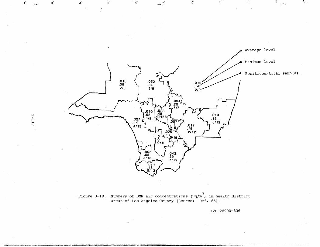
3.9.3 Atmospheric Survey of Nitrosamines--"'

Unlike most of the other pollutants considered on this program, a

systematic sampling for nitrosamines has been conducted in California.

This work, under CARE sponsorship, was done by R. J. Gordon of the USC

School of Medicine (Ref. 66). The survey included air sampling downwind

of: (1) the Teledyne UDMH plant (then operating); (2) the individual

chemical and petroleum plants situated between Richmond and Antioch; and

(3) selected points representing clusters of chemical plants (and a fish

processing plant) in the Vernon-Commerce and Carson-Wilmington districts.

Gordon also conducted a systematic sampling program in the southern half

of Los Angeles County at about 150 points for comparison with cancer

incidence datae I

* Linear alkylsulfonate. i KVB 26900-836

3-115

No evidence for any specific point emission source for volatile

nitrosamines was observed. The majority of all samples were below detection 3

limits (about 0.03 µg/m for dimethylnitrosamine (DMN). Several samples 3

reached 0.3 µg/m or higher, up to a maximim of 1.0 (for a mislabeled sample),

but later repeat samples were always lower. The second highest concentration 3

recorded was 0.48 µg/m; the sample was taken on the grounds of the Los

Angeles County Hospital.

Gordon concluded that more positive samples were collected in winter.

A diurnal pattern was suggested, with maxima around 8:00 a.m. and 6:00 p.m.

Diethylnitrosamine was found less frequently than DMN but at similar levels.

Traces of a third, less volatilel' unidentified nitrosamine r,11ere also seen.

Gordon's mapping of DM:N data in his cancer correlation study (no

apparent correlations found) are shown in Figure 3-19.

KVB 26900-836

3-116

......

E • Miscellaneous Other Secondary Amine Sources--

In the EPA report (Ref. 58), other sources of secondary amine emissions

were listed. These are: {1) systems disclosed in patents (amine-type

oxidation inhibitors for lubricants and rubber storage environment),

(2) synthetic detergent manufacture involving dimethylamine release, (3)

uranium oxide extraction with dilaurylarnine, and (4) leather tanning using

dimethylamine as a liming accelerator. Topic (1) was not pursued because

only patent literature was cited; this strongly implies uncertainty as to

whether reduction to industrial practice had occurred. Topic (2) concerns

the odor problem associated with the release of dimethylamine which occurs

as process contaminant in LAs"manufacture. According to Byrd et al (Ref. 65),

application of suitable APC equipment has elimil"!,ated this problem. This

was confirmed in discussions with Pilot Chemical Company of California,

a major LAS producer in this State. Topic (3), uranium oxide extraction

from yellow cake, was referred to the Bureau of Mines, Spokane, Washington.

According to that agency, there is no known uranium ore processing in this

State. The last topic deals with leather tanning and the use of dimethyl

amine (or sodium sulfide) as liming accelerators. The alkaline properties

of this (lime saturated) liquor would render the dissolved amine essentially

nonvolatileo

3.9.3 Atmospheric Survey of Nitrosamines--

Unlike most of the other pollutants considered on this program, a

systematic sampling for nitrosamines has been conducted in California.

This work, under CARE sponsorship, was done by R. J. Gordon of the USC

School of Medicine (Ref. 66). The survey included air sampling downwind

of: (1) the Teledyne UDMH plant (then operating); (2) the individual

chemical and petroleum plants situated between Richmond and Antioch; and

(3) selected points representing clusters of chemical plants (and a fish

processing plant) in the Vernon-Commerce and Carson-Wilmington districts.

Gordon also conducted a systematic sampling program in the southern half

of Los Angeles County at about 150 points for comparison with cancer

incidence dataa

* Linear alkylsulfonate. KVB 26900-836

3-115

No evidence for any specific point emission source for volatile

nitrosamines was observed. The majority of all samples were below detection 3

limits (about 0.03 l-lg/m for dirnethylnitrosamine (DMN). Several samples 3

reached 0.3 µg/m or higher, up to a maximirn of 1.0 (for a mislabeled sample),

but later repeat samples were always lower. The second highest concentration 3

recorded was O.. 48 µg/m ; the sample was tak,en on the grounds of the Los

Angeles County Hospital.

Gordon concluded that more positive samples were collected in winter.

A diurnal pattern was suggested, with maxima around 8:00 a.m. and 6:00 p.m.

Diethylnitrosamine was found less frequently than DMN" but at similar levels.

Traces of a third, less volatile, unidentified nitrosamine were also seen.

Gordon's mapping of DlYtN data in his cancer correlation study (no

apparent correlations found) are shown in Figure 3-19.

KVB 26900-836

3-116

~.-f if ,( .,' ic < •f c( '( "'l

,~-~.,.... --_ "

~ .0 t6 .08 218

Average level

Maximum level

Positives/total samples .

w I

I-' I-' -..J

3Figure 3-19. Summary of DMN air concentrations (µg/m ) in health district

areas of Los Angeles County (Source: Ref. 66).

KVB 26900-836

3 .• 10 PERCHLOROETHYLENE

3.10.1 Production-Usage Summary

Perchloroethylene (1, 1, 2, 2-tetrachloroethene), which is often

referred to as perc, is a widely used solvent. The modes of use, however,

are conducive to vapor release such that rather large emission factors have

been developed for perc sources.

The estimated 1978 National consumption of Pere has been tabulated

by SRI (Ref. 67). These data are shown b,elow with earlier (1971) usage

estimates compiled by Mitre Corp. (Ref. 68).

TABLE 3-29. ESTIMATED CONSUMPTION OF PERC IN THE U.S.

SRI Estimated 1978 % of Total Tn~e of Use Consumption, 106 lbs SRI-1978 Mitre-1971

Dry Cleaning 353 53 70

Textile Processing 44 7

Chemical Intermediate 88 13 11

.Metal Cleaning 110 17 18

Miscellaneous 66 10·" 1

661 100 100

* Includes Pere going into inventory.

The SRI study focused on only two use-categories (dry cleaning and

degreasing) and did not explain what consituted miscellaneous use, other

than suggested in the tab~e's footnote. In searching the EIS print-outs keyed

to perc emitters, no permitted sources could be identified that would fulfill

the miscellaneous category in California.

Use of perc as a chemical intermediate {Ref. 67) is predominately for

the syntheses of F-113 through F-116 (trichlorotrifluoroethane through

KVB 26900-836

3-ll8

hexafluoroethane). No facilities were identified in California that produced

other than fluorinated methanes (DuPont, Antioch and Allied Chemical, El

Segundo). Thus, it is assumed that chemical intermediate use of perc does

not occur in the State.

Use of perc in textile processing is insignificant in California. A

search of the EIS print-outs mentioned above, produced only a few hits (e.g.,

SIC 2283-Wool Yarn Mill; SIC 2262-Finisher of Broad Woven Fibers of Manmade

Fiber and Silk, etc.) for the category.

Thus, the present State survey, like the SRI National assessment, focused

on just three areas: (1) perc manufacture; (2) dry cleaning, and (3) degreasing

operations.

3.10.2 Pere Production ,._,

The only producer of perc in the state is Dow Chemical Co., Pittsburg.

According to SRI that plant has a ~ated annual capacity of 44 million lbs and

a production last year at half capacity, or 22 million lbs. 7hc process used,

w~ich also yields carbon tetrachloride, is described in Section 3.5.1.A.

3.10.3 Dry Cleaning

Three categories of dry cleaning operations can be considered:

Commercial dry cleaners--the common walk-in garment cleaning service

Coin-operated machines--located in self-service laund.r-ies, apart­ments, etc.

Industrial cleaners--supplying cleaned uniforms, wipe rags, safety equipment, dust control devices, etc .

......

SRI estimates that: (1) about 75% of commercial dry cleaners use perc;

C2) coin-operated dry cleaning machines use perc almost exclusively (3% use

F-113); and(3) about half the industrial cleaning plants are on perc. Except

for the small amount of F-113 used, the balance of cleaning fluid is believed

to be Stoddard solvent. The SRI estimated inventory of perc dry cleaning plants

in California, broken down by size of operation (based on nurnbe.r of employees),

is shown in Table 3-30.

KVB 26900-836 3-119

TABLE 3-30. ESTIMATED NUMBER OF DRY CLEANING PLANTS USING PERC IN THE U.S. AND CALIFORNIA

(Source: Ref. 67)

Number of Plants (% of Category Total)

No. of Employees Commercial Coin-Operated Industrial £er Plant U.S. Calif. U.S. Calif. U.S. Calif. --.,

1-4

5-9

10-19

20-49

50+

TOTALS

( 9., of total of all three categories)

4,194 (54. 1)

1,906 (24.6)

846 (10. 9)

691 (8.9)

119 (1. 5)

7,756

(62. 6)

566 (58.6)

247 (25.6)

101 (10.5)

44 (4. 6)

8 (0.8)

966

(72. 5)

3,695 (84. 3)

499 (11. 4)

119 (2. 7)

57 (1. 3)

12 (0. 3)

4,382

(35.4)

269 (80. 5)

47 (14 .1)

12 (3. 6)

4 (1. 2)

2 (0.6)

334

(25.1)

16 (6. 3)

11 (4. 3)

18 (7.1)

98 (38.4)

112 (43.9)

255

(2 .1)

3 (9.1)

2 (6 .1) ,_"

3 (9. 1)

12 (36.4)

13 (39.4)

33

~,

(2.4)

KVB 26900-836 3-120

....

While the distribution of types of dry cleaning establishments varies

somewhat between the Nation and the State, the conformity in size distribution

is reasonably good. This composition would then permit the calculation of

perc use in the State based on SRI's estimated national perc consumption and

the fraction of the national inventory of plants that are operating in the

State. This was done with the following results:

TABLE 3-31. ESTIMATED CONSUMPTION OF PERC FOR DRY CLEANING IN CALIFORNIA DURING 1978

- Estimated Pere % of Tyre of 0Eeration No. of Plants Consum,etion, 106 lbs Total Consumed

Commercial 966 33.8 78.7

Coin-operated 334 3.9 7.4

Industrial 33 4.0 13. 9

TOTALS 1333 41. 7 100.0

3.10.4 Metal Cleaning Operations

Solvent cleaning of metals can be dichotomized into two practices

cleaning with the hot vapor of the solvent and cleaning with the liquid

solvent itself, usually at room temperature. Thus, the terms "cold cleaning"

and "vapor degreasing 11 evolved. Application of these degreasing techniques

is predominately batch mode, although conveyorized configurations are dic­

tated for large output operations. The conveyorized degreasers may operate

as either cold cleaning or vapor degreasing systems.

KVB 26900-836

3-121

In batch cold cleaning, parts are suspended in a tank of solvent with

or without spraying, stirring, ultrasound~ and other process-accelerating

effects. Rejuvenation of the solvent is variously practiced ranging from

replacement of the discarded loaded solvent with fr,esh stock to distillation

of the dirty solvent and recycle.

In batch vapor degreasin~, the coated pieces are suspended in a vapor

reflux configuration. Under the load, the solvent is boiled and above the

load the solvent vapors are condensed on cooled surfaces. The clean reflux­

ate flows back into the pot while some vapor condenses on and drips off the

parts themselves, providing the cleaning effect. Most large vapor degreasers

are fitted with quick-operating lids and charcoal vapor recovery systems.

The most popular synthetj_c degreasing solvent is 1, 1, 1 - trichloro­

ethane (methylchloroform) followed, up w1.til recently, by trichloroethylene

and then perc. Halogenated solvents (the above three plus methylene chloride

and F-113) accounted for about 59 wt~% of the degreasing fluids used in 1974

(Ref. 68). The balance of the materials used in degreasers were petroleum

solvents (37 wt-%) and the various oxycarbons (4 wt-%).

Trichloroethylene, a photochemically active substance, is now falling

in popularity as a degreasing solvent in some states (certainly in California).

This has resulted from local APC regulation and, perhaps, the carcinogen-

icity issue. There is, however, no pending OSHA action for lowering the MAC

for trichloroethylene and the EPA is only now tentatively considering trichloro­

ethylene for inclusion on the list of hazardous pollutants. In any case,

most California degreasers who used that solvent have converted their tri­

chloroethylene degreasers to methylchloroform service. The boiling point

of the latter (74 °C) is closer to trichloroethylene (87 °C) than any of the 0

other halocarbon degreasing solvents. Pere (b. pt. 121 C) sales have also ap-

parently benefited somewhat from the reduced usage of trichloroethylene here.

Tr_e above observations resulted from discussions with technical representatives

of Baron-Blakeslee and Delta Industries, leading degreaser manufacturers.

In a study for the CARB, Eureka Laboratores (Ref. 69) canvassed a sampling

of California industries operating degreasers to determine solvent types used.

The field represented 45 different SIC codes, covering all possible categories

KVB 26900-8363-122

of degreaser users. Although the canvass reached only 5.8% of the selected

field, statistically this is a generous sample and should promote a high

confidence level in the results.

SRI (Ref. 67) analyzed the work sheets from the Eureka survey to

determine perc preference among the polled group. Some manufacturers in

17 of the 45 SIC codes canvassed were found to.degrease with perc. The

fractions within this subgroup using perc and their estimated annual conswnp­

tion of the solvent are shown in Table 3-32. KVB obtained from SRI (B.E. Suta)

the population of plants within the 17 SIC categories (according to size)

that SRI had extracted from the 1976 Bureau of Census report on 1974 County

Business Patterns.

This matrix represented a total of 6,550 plants that operated de­

greasers. The fraction using perc was then multiplied for each corresponding

population element and the SRI-estimated perc usage (Table 3-32) for that

particular SIC and plant size. The breakdown is shown in Table 3-33·-. Using

Mitre Corporation's (Ref. 68) estimated National consumption of perchloro­

ethylene for degreasing in 1975 (108 million lbs), the Table 3-32 estimate

for California is 11.9% of that total.

Several interesting aspects of the Table 3-33 perc consumption es­

timates are apparent. Small business operations using degreasers account

for a very minor part of the total. The aircraft and aircraft equipment

manufacturing industries account for almost 36% of the total degreasing perc

used. The larger companies (greater than 100 employees) account for over

67% of the perc consumed in degreasing, although only 62 plants comprise

that grouping.

A print-out from the Emission Inventory Subsystem (EIS) of firms

operating perc degreasers and dry cleaning equipment was also requested

and received from the CARB. 'l'hese data we.re fragmentary, there being no

information included for such important counties as most of those littoral

to San Francisco Bay. Although listed, no permits were recorded for Riverside

and San Bernardino Counties. Thus, the discrepancy in the total count of

KVB 26900-836 3-123

! I

11 I

I

! l

: I

11

I

TABLE 3-32. ESTIMATED FRACTIONAL AND INDIVIDUAL PLANT PERCHLOROETHYLENE USAGE FOR DEGREASING IN CALIFORNIA BY PLANT SIZE AND SIC TYPE

(Source: SRI and Eureka Laboratories - Refs. 67 & 69)

% Using Pere Amount of Pere Used

Per Plant, 10 3 ,lbs/yr

SIC Industry No. of Employees No. of Employees Code D~scription < 20 > 20 < 20 20-100 > 100

11

6

14

9

14

8

18

11

14

11

7

0

7

11

0

5

22

on number

0 24.4*

0 0.6*

0 163

0 36.0*

0 37.3

0 4.8

0 11. 7*

4.5 71. 3

0 17. 8

0 1. 2*

0 2.0*

3.0 0

0

0 2.4*

Jo. 0 0

0 1.5

0.14 6.6

of employees.

136

3.4

911*

200

209*

26.6*

65*

231

99*

6.8*

11.2

0

5.5

13. 3

0

8.4*

348

331

336

339

342

343

344

345

347

349

352

361

362

364

366

367

371

372

Basic steel 0

Non-ferrous foundry 0

Misc. primary metal 0

Gen. hardware 0

Plumbing and gas heating 0

Structural metal 0

Metal fasteners 0

Plating and engraving 8

Misc. metal products 0

Farm and garden eqpt. 0

Elec. transmission eqpt. 0

Elec. industrial apparatus 17

Elec. lighting and wiring 0

Communications eqpt. 0

Electronic components 6

Vehicles and eqpt. 0

Aircraft and eqpt. 10

* These estimates are extrapolations based

3-124 KVB 26900-836

TABLE 3-33. ESTIMATED TOTAL PERCHLOROETHYLENE USAGE IN CALIFORNIA DEGREASERS BY PLANT SIZE AND TYPE

lo,..,

Amount of Pere Used Per Category 103 lbs/yr

SIC Industry Number of Ernplo:iees ..... Code Description < 20 20-100 > 100

331 Basic steel 0 97 358

336 Non-ferrous foundry 0 3.2 5.5

339 Misc. prirna1."Y steel 0 911 637

342 Gen. hardware 0 191 774

343 Plumbing and gas heating 0 177 438

344 Structural metal 0 117 145

345 Metal fasteners 0 145 281

347 Plating and engraving 201 1,411 534

349 Misc. metal products 0 482 696

352 Farm and garden eqpt. 0 5.5 6.0

361 Elec. transmission eqpt. 0 4.7 17.2 ~,

( 362 Elec. industrial apparatus 53 0 0

364 Elec. lighting and wiring 0 6.3 15.7

366 Communication eqpt. 0 40.9 139

367 Electronic components 219 0 0 •.'--".

371 Vehicles and eqpt. 0 1.2 25.5

372 Aircraft and eqpt. 2.3 113 4,597

TOTALS 475 3,706 8,669

GRAND TOTAL 12,850,000 lbs '-

KVB 26900-836

3-125

degreasers shown in the EIS an.d the SRI data was expectable. For the South

Coast Air Basin, for example, the EIS lists only 128 degreasers, while the

SRI compilation shows about 250. The latter count represented a population

within a matrix consisting of 17 SIC (three digit) codes .. These were identified

by SRI within the 45 SIC codes canvassed by Excelsior Laboratories as in­

cluding any degreaser-operating companies employing perc. In the EIS print­

out, however, 41% of the SCABperc users involved SIC codes other than those

17. Of these extraneous sources, almost 60% did fall within the other 28

codes considered by Eureka. The balance were extraneous to the overall

matrix of 45 considered by that contractor.

While these overlooked SIC's represented 41% of the total permitted

and EIS-listed firms operating perc degreasers, emission-wise their contri­

bution was only 29% of the EIS total. If one assumes that there is a direct re­

lationship between perc consumption and release, then the total perc consump­

tion figure shown on Table 3-.]2 is possibly low by 29%. If this were the

case, total consumption of degreasing perc in California would be just over

18 million lbs/yr.

3.10.5 Enission Factors

A. Pere Production--

The Dow Chemical plant at Pittsburg is estimated by SRI (Ref. 67) to

emit 44,000 lbs/yr of perc. This is less than is released by a single, large,

open-top degreaser. The factor applied was 0.002 lb emitted/lb produced.

This factor was estimated for the direct chlorination process by the EPA

(Office of Air Quality Planning and Standards) on the basis of ''several very

limited studies of perc losses during production". The estimates were pro­

vided to SRI in a personal communication (December 1978) from J. K. Greer, Jr.

of that agency. An earlier SRI estimate {Ref. 70) placed the emission factor

at 7.5 times higher than that cited above.

Excerpts of the later SRI report were presented to Dow Chemical for

review. After studying the material, Dow returned the material without

comment.

KVB 26900-836 3-126

B. Dry Cleaning--

It is generally assumed {e.g., AP-42) that all of the perc consumed

by the dry cleaning business community is lost to the atmosphere. Based on 6

the Table 3-31 consumption estimate, this would amount to 41.7 x 10 lbs/yr

of perc emissions in California.

Fisher of the International Fabricare Institute (IFI) estimated

(Ref. 71} a per capita perc release of 1.75 and 1.99 lb/year based on report­

ed and calculated perc consumption, respectively. The Census Bureau estimated

the state's population at 22,294,000 as of July 1978. This would_represent 6

perc releases of 39.0 and 44.4 x 10 lbs/yr for the above two conditions. 6

The average of the two IFI estimates is 41.7 x 10 lbs/yr, which happens to

be the same value as calculated from Table 3-31•.

A CARB draft report (Ref. 72) dealing with solvent (petroleum and

synthetic) emissions from dry cleaning operations was obtained from that

agency. In the report, per capita emissions were estimated at 1.5 lb and

included both petroleum and synthetic species. This was based on AQMA

surveys of dry cleaning plants in the various jurisdictions. Although over

one-third of the state was not included, most of the state's population was

inclusive of the area inventoried. A survey was also conducted to determine

usage rates of petroleum solvent. This was found to average 3,840 gal/yr in

commercial plants and 37,200 gal/yr in industrial plants. Synthetic emissions

were calculated according to the following formula:

37,200 dE synth = 1. 5 p - (3,840 x d lb/plant-yr x :t'b) + { lb/

2

plant-yr x Ni )

where:

Nc = number of commercial cleaning establishments using petroleum

solvents

Ni = number of industrial cleaning establishments using petroleum

solvents

3-127 KVB 26900-836

p county population in 1976

d average density of petroleum solvent (6.5 lb/gal)·

The first term (1. 5 p) calculates the total petroleum and synthetic emissions

for the county (or State). The balance of the expression is intendeq: to

subtract out the petroleum solvent used in industrial and commercial operations

(coin-operated facilities can be ignored as using no petroleum solvent), and

then add back half the solvent consumed in industrial plants as being for the

cleaning of non-clothing items (drapes, rugs, uniforms, cleaning rags, etc.).

It was apparently assumed that the 1.5 lb per capita emission factor did only

include solvent releases from wearing apparel.

The formula, however,, fails to accomplish the stated scenario. While

the second term does subtract out petrol,eum solvent usage in commercial plants,

the third term does not accomplish this for industrial plants or add back

half the synthetic solvent used to clean non-clothing items. As written,

the formula defines estimated emissions to include all the synthetic solvent

used in all dry cleaning operations plus 150% of the petroleum solvent used

in industrial facilities.

A breakdown by county of perc emissions was included in the CARE 6

report (Ref. 72). The total for the entire state was 27.4 x 10 lbs/yr.

The estimate may be on the low end of the probable range.

The distribution of the .sources responsible for these considerable

perc emissions are doubtless consistent with population densities. The small

(approx. 14%) fraction of the total perc emitted by industrial cleaning

establishments is probably concentrated in non-residential zones of the major

California cities. The general effect, however, should still be one in which·

perc dry cleaning emissions are distributed according to and are directly pro­

portional to urban population concentrations.

C. Degreasing Operations--

The EPA (Ref. 73) estimates the average emission rate for cold cleaners

at 662 lbs/yr, although the rates vary widely. Most losses occur-because of

KVB 26900-836 3-128

bath evaporation, solvent carry-out, agitation, waste solvent evaporation, and

spray evaporation. In sharp contrast, the same report estimates the average

solvent loss for an open top vapor degreaser at 80,650 lb/yr. Most of the

losses are directly out of the opening, there being relatively small losses

occasioned by carry-out or waste solvent evaporation. Conveyorized degreasers

are mostly of the vapor type, only about 15% being designed to operate with

cold solvent. Although typically of larger capacity, the conveyor vapor de­

greasers are of enclosed design and thus release less solvent than the open

top configuration. The EPA estimates the average conveyorized vapor degreaser

to emit 55,620 lb/yr of solvent. The cold conveyorized degreasers are estim­

ated to release about 105,000 lb/yr per unit on the average. The more recent

designs are far more efficient, however.

The EPA report estimates that only 10 to 20% of the solvent i_nput to

conveyorized degreasers and 20 to 25% of the solvent input to open top vapor

degreasers are disposed of as waste solvent. In California, most vapor de­

greasers distill and recycle this material in-house. APCD pennit charges are

based on solvent purchases The incentive is thus to recycle solvent internallY,

rather than to sell off dirty solvent to outside reclaimers, according to the

degreaser manufacturers cited earlier.

Emissions from degreasing operations are ge.nerally regarded (e.g. ,

AP-42) as being equal to the solvent purchased. The Eureka study (Ref. 69)

subtracts out solvent sent to reclaimers, which involved a small fraction.

Mitre Corp. (Ref. 68) estimates that 98% of the solvent purchased is Jost

to the atmosphere.

The Eureka study, which involved the polling of a generous sampling ......

of degreaser users, resulted in emissions for nine different solvents in the

principal California air basins by 45 SIC plant categories. The latter was

assumed to embrace all probable classifications that would be employing

degreaser equipment. As pointed out earlier, this is not the case, but the

error involved is not great. The results obtained by Eureka for perc emissions

in 1976 are given in Table 3-34. They have also been cited in a recent CARB

model rule proposed (Ref. 74) within that agency.

KVB 26900-836 3-129

TABLE 3-34. ESTIMATED PERC EMISSIONS FOR MANUFACTURING INDUSTRY DEGREASING OPERtt\.TIONS FOR 1976

(Source: Eureka Laboratories, Ref. 68)

Pere Emissions, Air Basin County 103 lbs/yr % of State

Sacramento Valley Sacramento 14.6 0.09

San Diego San Diego 1,343 8.1

San Francisco Bay Area Alameda 263 Contra Costa 21.9 Marin 197 Santa Clara 453 San Francisco 58.4

TOTAL 993 6.0

San Joaquin Valley Fresno 29.2 Kern 7.3 San Joaquin 321 Stanislaus Tulare

TOTAL 358 2.2

South Central Coast .Santa Barbara 307 Ventura

TOT~l\L 307 1. 9

South Coast Los Angeles 11,592 Orange 1;854 Riverside 29.2 San Bernardino 80.3

TOTAL 13,556 81.8

State total 16,571,600 lbs/yr.

------------·-=======-...::.====================================

KVB 26900-836

3-130

It will be noted that the State total emissions of perc are consider­

ably larger than the consumption rate estimated in Table 3-33. The data

presented in that table are, however, based on SRI statistics which consider­

ed only 17 of the 45 SIC codes canvassed by Eureka. SRI felt that all of the

perc users were inclusive of that grouping. As pointed out earlier, it was

estimated that their figures may be low by 29% because, based on SCAB perc

emissions data (EIS),rnany other SIC categories had been overlooked. Thus,

if the Table 3-33 data are increased by 29%, the estimated release for the 6state would be 16.58 x 10 lbs/yr. This extremely close agreement with the

6Eureka estimate (16.57 x 10 ) is extraordinary. Although SRI worked with

Eureka's questionnaire results, KVB adjusted the Table 3-33 total using EIS

emission factors (and for only one air basin) rather than Eureka's findings.

The one air basin -- SCAB -- does, however, furnish an estimated 81.8% of

the total perc emissions in the state.

Just 90% of the total perc emissions are identified with four counties:

Los Angeles (70.0%), Orange (11.2%), San Diego (6.0%), and Santa Clara

(2.7%).

Because of the high concentration of perc emissions in Los Angeles

County, the EIS printouts were searched to detect the possible existence of

hot spots. It was noted that 12 aircraft/aerospace and two other companies

were responsible for 22% of the perc emissions in the County. Of that

fraction, 45% were contributed by one firm, the Day and Night Manufacturing Co.,

City of Industry (SIC 3822 - automatic controls for regulating residential

and commerical environmental control systems and related appliances). The

annual release of perc from that plant is listed as 1,180,000 lbs/yr in the

EIS. These sources are plotted on Figure 3-20- The distribution of the

balance of the perc degreasers generally covered the industrialized areas

of greater Los Angeles.

D. Ambient Air Measurements--

In 1972, Simmonds, et al (Ref. 75) obtained ambient perc measurements

on three different dates at mostly non-repeated station sites throughout

3-131 KVB 26900-836

)

w I

I--' w N

Canoga Park -Rockwell c1s;ooo)

Santa Monica -Gillette Co.-(2-38-,-o-o'o)

Palmdale - Lockheed (80,000)

Burbank - Weber Aircraft (128,000) Lo,· :,eed (240,000)

Commerce - Lockheed (224,000)

Compton - Air Form {44,000)

Industry - Day & Night Mfr. Co. (1,180,000)

Downey - Rockwell (12,000)

<160 -.so aoo 020

~---/<:J= I I I 'f l l//h4 I /I I I I I I I I I !1710Inglewood -Western Airlines (42,000)

Manhattan Beach -Fairchild Aircraft (56,000)

Redondo Beach"-------J TRW, Inc. (32,000)

Torrance -Airesearch (86,000) Aeronca (260,000)

)

Selllwr,cr11i,.i

- I I 4-=F=r~ ~, 1 ~A=11 1 rr , , )1"~,.~ neo

H-1

~:

\ Figure 3-20. Location of 14 degreaser-operating firms estimated to be

contributing 22% of the perchloroethylene released in Los Angeles County by such operations (emission factors in lbs/yr).

KVB 26900-836

) ) _,/ ) ) ) )

Los Angeles County. On a fourth date, samples were taken in the San Bernardino

Mountains-to characterize background. The weather conditions were somewhat

mixed. In the first survey (industrial eastern Los Angeles), perc levels

ranged from 1.3 to 2.5 ppb. The second survey ranged from the area of the

first survey west through central Los Angeles to Santa Monica Bay. At the

beach station a value of 0.01 ppb was obtained, while the high value proved

to be 3.8 ppb (central Los Angeles). The third survey ranged south into

Orange County, triangulating from the extreme eastern and western stations

of the first two surveys. On the third survey, perc levels ranged from

0.06 ppb (west central Orange County) to 3.84 ppb (at the coast). The 24 hr

average obtained at about 6,000 feet in the San Bernardino Mountains was

Oo09 ppb.

The one station (industrial eastern Los Angeles) that was sampled

on all three surveys produced an average for the three samples of 1.4 + 0.3

ppb perc. This site, incidentally, was probably less than ten miles distant

from the Day and Night Manufacturing Co. plant, which alone is estimated to

realease 7% of all the perc emitted by degreasers in the state.

KVB 26900-836

3-133

,,I

I

.....,,

3.11 POLYCYCLIC ORGANIC MATTER l[POM}

3.11.1 General Nature of the Pollutant Category

A. Definition--

Some confusion exists as to the specific chemical class(es) repre­

sented by the POM category. The tendency is to assume. that the precedent

expressions PAH, PNAf and PNAH are all the same classification. The latter

three abbreviations refer, however, to fused polycyclic (polynuclear) hydro­

carbons (carbon and hydrogen only) which exhibit a maximum number of

non-cumulative double bonds (or aromaticity). The narrowness of this classi­

fication is raised since saturated and heteroatomic derivations of the poly­

nuclear aromatics certainly occur with them in the polluted media. Such other

forms, perhaps no less potent carcinogens, are therefore brought into the

category, the definition of which has been semantically broadened under the

title, 0 Polycyclic Organic Matter.''

The National Academy of Science :first used the title (Ref. 7,J ), and

the EPA eventually defined it {Ref.77 ). This definition is somewhat confus­

ing because of the terminology used. Included in the POM category are the

true PNA's, plus aza and imino (the terms are synonymous), arenes (generic

term for monocyclic as well as fused ring aromatic hydrocarbons),and so on.

The intent, however, was to bring in a broader class of compounds that allows

nitrogen,. oxygen, sulfur, and oxycarbon ring-atoms as well as PCB I s and ap­

propriate pesticides. The last two subgroupings were not considered in the

present study. Collectively, PCB's now comprise a banned substance category.

Pesticides represent a commodity rather than a chemical class. Many pesti­

cides could be shown to fit the imprecise EPA definition of POM, the

determination of which would clearly be outside the int,mt ot the study.

*The expression PNA will be used in this discussion to refer to the true hydrocarbon fused ringed aromatic compounds.

KVB 26900-836 3-134

B. Occurrence--

With the exceptions of PCB's and pesticides, the use of technical-grade

chemicals that are generically POM's is limited to a few materials in commerce.

Very small amounts of true PNA's are used as organic semi-conductors. In the

broader POM concept, cholesteric liquid crystalline materials can be considered;

they are widely employed in numeric registers for calculators and wrist watches.

Naphthalene (the simplest fused ring aromatic but not a polynuclear aromatic)

is heavily used (75% of that produced) in the synthesis of phthalic anhydride,

dyestuffs, and various specialty chemicals (Ref. 59). California apparently

does not share in this area of manufacture.

The principal occurrence of POM arises as a result of combustion

processes. Minor releases are associated with ~sphalt-product manufacture,

carbon black production, bauxite reduction, and tire-wear (carbon back re­

lease)8 according to the EPA (Ref. 77).

In combustive processes, the major concern, POM's are typically

pyrogenically formed. Benzene itself is very refractory and can survive

thermal environments in which other hydrocarbons completely oxidize. The

presence of this aromatic in a reactive zone with nonaromatic radicals can

produce accreted, cyclized structures. These can then molecularly condense

with each other to produce a wide variety of fused ring species. On leaving

the hot zone of the sponsoring process, the POM vapors must physically con­

dense, which process is promoted by any particulate matter capable of nuc­

leating the effect. Ordinary soot or fly ash from boilers, Diesels, jet

engines, forest fires, etc., serve this function.

c. Measurement of POM--

The measurement of POM's is also an imprecise if highly challenging

technical art. It is virtually impossible at the present time to identify

and quantify all of the class species in any given POM sample. It is also

quite inadequate to apply many of the extant sampling techniques to the col­

lection of these substances, and expect 100%·recovery for analysis. This

situation is generally acknowledged by the community of analytical chemists.

KVB 26900-836 3-135

The family of chemical analytes comprising P0M's is simply too

numerous, too extensive of range in physical and chemical properties, and

so involatile at the higher boiling end that it frustrates facile specific

analyses.

At present, considerable POM testing is being done with the com­

puterized GC/MS. This is a semiquantitative analysis which furnishes

reasonable resolution of species but shows deteriorating recovery as molecular

weight and/or polarity of the eluted compounds increase. High performance

liquid chromatography (HPLC) is suggested for more accurate results. It is a

more reliable quantitative procedure and does tend to overcome the inadequacies

of GC/MS in eluting the lower vapor pressure POM 1 s. HPLC does not furnish

the resolution available from an efficient (60,000 to 70,000 effective theoretical

plates) capillary GC colLwnn. It also cannot identify the substances triggering

the detector (s). Analysis is thus an inadequately developed art for this

difficult mixture of chemicals tha~ until recently, was of relatively little

interest to the analyst.

Because the P0M family is a very complex chemical group and the

analytical chemistry being applied is far from optimum, compromise procedures

have been adopted. A favored technique is to measure the PNA, benzo[a]pyrene

(Ba.P) as being the representative or "surrogate" for the entire class. This

resulted because BaP analysis was theretofore reasonably developed, favorinq

its use as an indicator P0M s®stance.

In some cases, the values of BaP determined for a particulate sample

can be related to data available from the same sampling for benzene soluble

organics {BS0) and a fraction loosely defined as "P0M''. The last is usually·

the sum of ten (and sometimes more) PNA species (pyrene 1, BaP, BeP, perylene,

benzo[ghi]perylene, anthracene, caronene, anthranthrene, phenanthrene, and

fluoranthene) collected on the front and back portions of the EPA Method 5

sampling train. While this group of ten PNA's does not possibly represent all

of the P0M in the sample, the BSO will conversely include most or all of the

POM but other matter as well. Thus, the actual P0M content lies somewhere between

the yield of ten or more PNA 1 s and BS0. A comparison of BaP values with BS0

and the totalled PNA's will afford the extremes of the range in which the ratio

of BaP to POM should fall. These data are shown in Table 3-35.

KVB 26900-8363-136

-TABLE 3-35 ESTIMATES OF RATIOS FOR BaP, BSO, AND TEN

PNA's FOR VARIOUS PROCESSES BASED ON GEOMETRIC MEANS. OF COLLECTED DATA

Process BSO/BaP PNA' s */BaP Reference

Coke Production Wet coal charging 500 Quenching 300 Door leaks 167 Battery stacks 133

Residential Fireplaces...... (Wood burning)

Oil Fired Intermediate Boilers Steam atomized 80,900 Low pressure, air atomized 15,500

Forest Fires ...... Heading Backing

Mobile Sources Autos (diesel) 3,250 Trucks (diesel)

Gas Fireq Intermediate Boilers Process steam > 800 Hospital heating 2,760

Gas Fired Residential Heaters Double shell boiler 19,500 Hot air furnace 11,000 Wall heater 20,000

Petroleum Catalytic Crackers# Regenerator outlet 12,160 CO waste heat boiler > 89,000

Asphalt Production Saturators (controlled) Air blowing (controlled) Hot road mix (controlled) > 180,000

28

21 21

810

> 3.5 145

23 13

110

68 24

4 50

> 70

78 78 78 78

79

80 80

81 81

82 83

80 80

80 ,I80

80 !

80 80

84 84 80

* Ten I'Nl\'g were dctcrr.i.incd and sur.uncd unlcs!:. "i"

Fourteen PNA's determined and summed.

§Eighteen PNA's determined and summed. #All types weighted by population.

otherwise specified.

3-137 KVB 26900-836

l I

D. POM Emission Sources--

Some 17 categories of POM sources have been identified by Energy and

Environmental Analysis, Inc. (EEA) as emitters of POM {Ref. 85). A number

of these source types do not exist in California or are so limited in number

as to be inconsequential. These sources include coal-fired power plants,

industrial boilers, and residential furnaces; municipal and commercial in­

cinerators; bauxite reduction plants; open burning dumps; and burning coal

refuse b~nks. The balance of the source types and the estimated National

emissions of BaP included in the EEA report are shown in Table 3-36.

These estimates are described as being quite coarse by EEA. Also,

by utilizing BaP as the indicator or surrogate substance, the actual POM

emission factors are speculative and certainly considerably higher. Nonetheless,

concern for all source categories listed in Table 3-36 below "Iron and Steel

Sintering" can be dismissed as minor in nature by comparison.

In the higher BaP emission categories, the estimates point to dispersed

sources in all cases except the dominant one. This is coking for steel pro­

duction and the related practice of iron ore sintering. In California, this

occurs at only one site, the Fontana steel mill of the Kaiser Steel Co.

Although the estimated POM emissions for coking shown in Table 3-36 are National,

one must assume that, until source testing is accomplished, releases at Fontana

are proportional in terms of coke output.

Another factor in coking to be noted is that the BSO/BaP and PNA/BaP

ratios for coking operations are the lowest for any of the source categories

shown in Table 3-35. This suggests, although not convincingly,considering

the measurement methodology, that coking oven POM emissions are comparatively

enriched in BaP with respect to other types of POM species.

Whatever attention again focuses on the Kaiser plant in this present

topic, the other designated POM sources should also be considered. The next

section therefore deals with all the categories listed in Table 3-36 with

the exception of those previously eliminated as being minor in nature.

KVB 26900-836

3-138

TABLE 3-36- ESTIMA'I'ES OF TOTAL BaP EMISSIONS IN THE UNITED STATES BY SOURCE TYPE

I...,

(Source: Energy and Environmental Analysis, Inc. - Ref. 85)

Estimated BaP Emissions, Tons Annual Production Date Geometric

....., Source or Fuel Consumption Year Minimum Maximum Mean

Ii..,

. (

6Coke Production 56.5 X 10 tons

6Residential Fireplaces 47.5 X 10 tons (wood)

Oil Fired Intermediate Boilers 6

Commercial/ 522.6 X 10 tons Institutional

Industrial 377 .1 X 106 tons

Forest Fires 8,000 sq miles

Mobile Sources Tire wear 217 X 106 pop'n Motorcycles 512 X 106 gals Autos (gasoline) 78 X 109 gals Autos (Diesel) 10 X 106 gals Trucks (Diesel) 9 X 109 gals

Iron & Steel Sintering 40.8 X 106 tons

Gas Fired Intermediate Boilers 1012Commercial/ 2.8 X cu ft

Institutional 12Industrial 5.3 X 10 cu ft

1012Gas Fired Residential 7.6 X cu ft Furnaces

1975

1975

1973

1973

1976

1977 1975 1975 1975 1975

1977

1973

1973

1973

0.06

57

0.25

10.5

0

1. 7 0.007 0.009

0.024

0.13

330 120

120 80

21

0.75 0.41

140 110

12 6.2

3.6 3.0 0.03 0.01 6.8 0.14

45 0.69

0.67

0.02

1.7 0.47

I....,

.....,

Petroleum Catalytic Crackers 6

Fluid cat 28.8 X 10 cu ft Thermofor 1.6 X 106 cu ft Houdriflow 0.1 X 106 cu ft

Carbon Black Production 1.3 X 106 tons

Asphalt Production Saturators 4.8 X 106 tons Air blowing 4.8 X 106 tons Hot road mix 21.5 X 106 tons

1977 1977 1977

1976

1976 1976 1976

0.00002 negl

0.043

negl 0.002

0.003 0.0003 0.04 0.001

0.005

0.096 0.096

0.019 0.005 0.027 0.005 0.014 0.001

!1

:I

3-139 KVB 26900-836

I I

,i ,, I

3 .11. 2 Emission Factors

A. Coking Operations and Ore Sintering~-

The coal and coke estimates developed by SRI (Ref. 86) show 1975 coke 6

production at Fontana at about 1. 3 x 10 tons. This was produced in 315

ovens organized within seven batteries. Comparing this coke production w,ith

the National output and the average BaP (Table 3-36) emission, the factor

for Fontana would be 5,500 lbs/yr of BaP. The ratios given in Table 3-35 would

suggest that the release of PNA's (14 species, including BaP) would be about

three times that amount, and of BSO about 300 times (based on a rounded average

of Table 3-35 BSO/BaP ratios).

B. Residential Wood Burning Fireplaces--

As the Table 3-36 estimates suggest .. the burning of wood is a relatively

rich source for the emissions of POM. This may arise from the aromatic nature

of lignin, a characteristic fraction of woody plants and trees.

Of the sources listed in Table 3-36J, the home fireplace emerges as the

third largest source of BaP emissions in the United States. Assuming that

California homeowners burn wood in the fireplaces in proportion to their

fraction of the National population (~10%), then the BaP emissions from these

sources would be 16,000 lbs/yr --poM. The Califon~ia Housing and Comi."lluni ty

Development Department estim?ted that, as of January 1978, there were 8,613,388

residential units in the State. Although not all of these housing units have

fireplaces, a fireplace emission factor of 840 mg BaP/yr. per unit is calcu­

lated. This is based on the data given in Ref. 79 for ten PNA's measured in

home fireplace emissions. Assuming that these ten PNA 1 s {including BaP) re­

present the entire POM class, then the POM emission factor would be 23.7 g

POM/yr per unit. The BaP fraction in the ten PNA's measured was 3.54%.

KVB 26900-8363-140

c. Oil Fired Intermediate Boilers--

The two types of boilers considered in this class, as shown in Table

3-36, are industrial and institutional/commercial boilers. The former are

employed in manufacturing processes to furnish process steam and electricity. 6

The industrial boilers are of higher energy capacity (> 20 x 10 Btu/hr) and

are more efficient combustors than the smaller institutional/commercial ..... boilers c~ 10 x 10

6Btu/hr). As shown in Table 3-36, the BaP emissions of

industrial boilers are relatively low even though their fuel comsumption is

similar to that of institutional/commercial boilers. Their emissions are also

a small fraction of the total and are therefore not considered further.

The institutional/commercial boilers are typically low pressure, air­

atomized devices that are used for space heating. In California, most are

operated with natural gas although all must have standby oil firing capability.

When gas service is interrupted, the oil systems are of course used. Practically

all boilers in this category purchase gas at curtailable service rates.

Curtailment is very infrequent, however, such that oil firing occurs for only

several days a month during the winter months. Thus, the State's fraction

of the oil burned in these smaller boilers throughout the nation (523 million

tons, per Table 3-36) is far below the population ratio. For this reason,

development of an emission factor was not attempted.

D. Forest Fires--

Considerable variability in the output of POM is seen in burning timber

stands (Ref. 81). Smoldering fires emit three to four times the BaP as do

flaming forest areas. Fires burninq into the wind (backing) emit eight to ten

times the BaP as do wind-driven (heading) fires. These ratios are considerably

higher for the comparative yields of PNA's (18 determined in the case of the

data considered here). The estimated average emissions for forest fires are

therefore quite coarse.

In Table 3-36 the area consumed by forest fires is listed at 8,000

square miles in 1976. Comparative forest area loss in California is con­

siderably less than the National population ratio. The six year average fur­

nished by the State Dept. of Forestry includes all State fire control juris­

dictions (California Dept. of Forestry, U.S. Forestry Service, Bureau of Land

KVB 26900-836

3-141

Management, U.S. Park Services, and five counties contracted to protect State

forests), is 378 square miles annually destroyed. This is less than 5% of the

National loss figure.

This fractional area loss figure permits estimation of BaP emissions

in the amount of 10,400 lbs/yr based on Table 3-36. The amount of PNA 1 s

that would be measured (18 species including BaP, according to Ref. 81) would

weigh somewhere between 50 to 250 times as much.

E. Mobile Sources--

1. Tire wear--The National Academy of Science (NAS) points out (Ref. 76)

that the carbon black (a rich source of PO.M) incorporated in vehicle tires

as opacifier releases that matter with wear. Relevant statistics on parti­

culate releases are cited in Section 3.4.6C of this report. The NAS estimated

emissions range from zero to 12 tpy (Table 3-36}. The California fraction,

based on vehicle population would be less than 3,000 lbs per year. The effect

would be highly dispersed.

2. Motorcycles--Most lower horsepower motorcycles are equipped with two

cycle engines. These engines combu.st a premixed fuel of gasoline and oil.

Combustion is less efficient than that in a four cycle engine since the

exhaust remains in the firing chamber after each cycle. 'I'he presence of oil

results in high emissions of POM (Ref. 76).

The NAS estimates the national release of BaP from motorcycles at

6.2 tpy. Assuming the state motorcycle population ratio to National count

corresponds with the human population ratio of about 10%, the BaP release from

this source in California would be less than one ton per year.

3. Other vehicles--The POM emissions of gasoline engine automobiles

have been characterized by Gross (Ref. 87). Based on his data and the estimates

for gasoline consumption, the release shown in Table 3-36 was derived by EEA

{Ref. 85). The fractional amount released in California would be about 1,000

lbs/yr, roughly one-half the amount released by motorcycles. This is notable

in that automobiles consume over 150 times the gasoline used in motorcycles.

KVB 26900-836 3-142

The contributions of Diesel engines to the POM burden are minor.

What is interesting in the estimates presented in the Table 3-36 is the

disparity of emission factors between the gasoline and Diesel engine auto­

mobiles and trucks. On a unit volume of fuel, the Diesel truck emits only

40% of the BaP attributed to the gasoline engine car. The latter, in turn is

estimated to produce only 2.5% BaP of the Diesel car. Per gallon, the

latter emits 90 times the BaP than does a truck equipped with the same type

engine.

3.11.3 Ambient Levels of BaP and BSO

As might be expected from the previous discussion, POM emissions of

integrated steel plants are of greatest concern. Thus, average BaP and

BSO data obtained from the National Air Surveillance Network {NASN) are

compared with respect to cities in which such mills are located to those not

hosting such operations. This comparison was prepared by SRI {Ref. 74) and

is shown in Table.s 3-37 and 3-38.

These data can be compared with the levels measured at seven Southern

California cities, all of which are 75 miles or less from Fontana (Table 3-39).

The data suggest several things. Emissions of POM, as indicated by BaP

measurements may have dropped over the past decade. The levels of ambient BaP

in U.S. cities hosting coking plants appear to be higher than in those which

do not.

KVB 26900-836

3-143

TABLE 3-37. SUMMARIZATION OF NATIONAL AMBIENT BaP AND BSO DATA FROM NATIONAL AIR SURVEILLANCE NETWORK (NASN)

Cities with Cities without Pollutant Statistic Coke Ovens Coke Ovens Rural Areas

BaP (ng/m3 ) 1975 data Average 1.21 0.38 < 0.10

Sample size* 21 13 3

Range 0.3-4.7 0.03-0.9 < 0.10

BSO (JJg/m3) 1971-72 data Average 4.21 3.75 0.95

Sample size* 25 12 2

Range 2.1-7.3 1. 9-5. 6 0.8-1.1

* Number of cities providing averaged annual concentration data.

Source: Ref. 85

TABLE 3-38 ~ CHRONOLOGICAL BaP AVERAGES FOR SELECTED U.S. CITIES (NASN DATA) (ng/m3 )

Cities with Cities without Year Coke Ovens Coke Ovens

1966 4.74 (15) * 2.76 (7)

1967 5.34 (15) 2.29 (8) _...,,_

1968 3.75 (18) 2.64 (8)

1969 4.41 (23) 2.14 (11)

1970 3. 02 (21) 1.41 (11)

1971 2.18 (11) 1. 22 (8)

1972 2.14 (19) 0.64 (11)

1975 1. 21 (21) 0.38 (13)

1976 0.93 (20) 0.41 (13)

* Number of cities included in average.

Source: Ref. 85

KVB 26900-836

3-144

TABLE 3-39. ATMOSPHERIC BaP AND BSO CONCENTRATIONS FOR CHESS AND CHAMP SITES IN CALIFORNIA*

3 3Distance from BaP (n9:/m } BSO (µg/m }

Location Fontana, Miles Mean Ran9:e Mean Range

Vista 65 1.03 0.1-4.9 2.07 0.8-6.7

Santa Monica 64 1.46 0.2-3.5 3.91 1. 1-6.1

Thousand Oaks 75 0.63 0.1-1.4 2.31 1.1-4.8

Garden Grove

Glendora

West Covina

Anaheim

37

23

29

34

2.42

0.91

1.98

2.36

0.3-7.5

0.1-2.2

0.2-5.0

0.4-7.1

3.86

4.13

5.85

4. 77

0. 8-11. 9

0.5-6.5

2.6-9.5

1.6-11.2

* Data collected in 1975 over a 12 month period (except Santa Monica, which was for six months}; all samples are 24 hour averages.

Source: Ref. 85

The pattern in Southern California for seven cities in 1975 shows

BaP at,ld BSO levels that are higher than the National average for cities 3 3

having steel mills (BaP 1.80 vs 1.20 ng/m and BSO 4.40 vs 4 .. 21 µg/rn, re-

spectively). The effect of the Fontana coking plant in this is not clear.

The CHESS/CHAMP data are for cities off the prevailing wind (westerly) at

Fontana. Glendora, the nearest city to Fontana exhibits the next to lowest

BaP value for the ~et. It would be of interest to measure BaP levels east

of Fontana at, say, San Bernardino or Redlands.

I

i I

KVB 26900-836

3-145

I·

1

SECTION 4. 0

POPULATION DENSITIES RELATIVE TO POLLUTANT SOURCES

4.1 SOURCE MAPPING

A number of the pollutants studied were found to be used in a manner

that resulted in their being released as area sources. Figure 1-2 presented

early in this report was included to show this effect for sources exhibiting

some geographic definitions. Other pollutant sources considered are so

highly dispersed, however, that even this treatment is not possible.

In contrast to the dispersed area sources that offer no reco:,nizable

''hot spots," a number of materials and point sources were described. Assuming

that the emissions factors associat,ed with these point sources are significant,

these can be mapped to show relationship with population density. This has

been done here using a Bureau of Census map (stock no. 0324-00214) section.

In ry,rerlaying the point sources of interest, a single map was

originally considered. This proved too cluttered.r so that two separate maps

have been prepared. The display of "hot spots'' on the two maps was arbitrar­

ily segregated in-co displays of sources for the inorganic and organic classes

of materials. Explanatory tables furnish firm names and estimated emissions

rates. The technique for reading the population density map was given earlier

with Figure 1-2.

In the following discussions, comments are also offered on the mic:::-o­

meteorology /topography of the locales in which various souces or groups of

sources are situated. These observations derive from the general knowledge

of the project staff and should not be construed as being products of the study

itself.

4-1 KVB 26900-836

4.2 INORGANIC POLLUTANTS

4.2.1 Arsenic

From Figure 4-1 and Table 4-1, it can be seen that 90% of the arsenic

emissions emitted (mostly from the secondary lead smelters) is released

into the South Coast Air Basin (SCAB). Most of the pollutant is released

in the heaviest populated area of the State. The topography of the basin and

its historical lack of air qrainage are well known. The balance (10%) of the

arsenic released in the State is from reasonably well ventilated shore

sites.

4.2.2 Asbestos

All three of the asbestos mining and milling areas are located in

very lightly populated areas, although each is near a small city or town.

The micrometeorology and topography in each case favors the dispersion

of particulate matter. This probabl~ is not altogether an advantage in view

of the great amount of surface-exposed facies bearing asbestos.

4.2.3 Cadmium

This air pollutant is· associated principally with the Kaiser steel

mill at Fontana. Also located in the SCAB, this locale suffers from deficient

vertical air movement and prevailing (light) winds are westerly. The

topography comprising a tank framed by the (clockwise) San Gabriel, San

Bernardino, San Jacinto, Lakeview, and Santa Ana Mountains, entraps polluted

air masses in the moderately populated areas around San Bernardino, Redlands

and Riverside. The Kaiser mill contributes cadmium (,and three other of the

materials of interest)to this pocket of polluted air.

Another source of significant cadmium emissions is the highway vehicle

tire. Conceptualization of traffic density patterns with respect to popu-

lation densities was given earlier in Figure 1-2. This map overlay, however,

KVB 26900-836

4-2

......

P,sbestos (11..--

it\,sbestos

Arsenic

Inorganic Pollutants

Arseri i '- {4if,

Arsenic (8_)_/4,miurn

( 3)

·C

4--1. Location of inorganic carcinogen emission sources relative i<) California population concentrations. KVB 26900-836

4-3

I

......,.

TABLE 4-1. INORGANIC POLLUTANT SOURCE INFORMATION CORRESPONDING TO FIGURE 4-1

EstimatedMap Type AnnualCode Fi1'111 Name Operation Emissions! Lbs ARSENIC 1 Antioch Pac. Gas & Elect. Pwr Plt 1,225

Pittsburg 2,0852 Morro Bay 1,1723 Oxnard So. ca 1. l::dison 1.189 4 Redondo Beach 1,134

El Segundo 809..Hernosa Beach 645

...., (

ASBESTOS

CADMIUM

5

6 7 8

1 2 3

1

Long Beach Seal Beach Carson Vernon Carlsbad San Diego San Bernardino Etiwanda Fontana

King City Coalinga Coppetopolis

Fontana

LA Dept W&P ALCO Pacific Gould, Inc. San Diego G&E

Southwest Smelt. So. ca1. Edison Kaiser Steel Co

Union Carbide Atlas ASbestos Calaveras Asb

Kaiser Steel Co

Lead Smelt.

Pwr Plt

Lead Smelt. Pwr Flt Steel Mill

Ash.mine

Steel Mill

1,561 1,216 4,400

44,000 677 744

4,400 800

1,480

26,500 17,500 34,000

14,000

i

'\•.. -- ,i !

KVB 26900-836

4-4

shows flow densities for only the State highway systems. This represents

roughly half the highway miles driven. The other half, operated by county

and city jurisdictions, lies mostly within the densest population zones.

KVB 26900-836

4-5

l

4.3 ORGANIC POLLUTANTS

4.3.l Benzene

Before considering the point sources emitting this chemical, the

reader is again referred to Figure 1-2 As pointed out earlier, the auto-

mobile is a major source of benzene pollution.

The "hot spots" identified with benzene emissions are the tvro producers

(ARCO-Carson and Chevron - El Segundo), the three benzene converters (Chevron-

El Segundq,Chevron-Richmond and Witco-Carson), the refinery community

and the Kaiser steel plant. These are shown on Figure 4-2 with emission

factor tabulations included in Table 4-2. With the estimated high release

from the Kaiser plant, together with emissions from thirteen refineries (two

of which produce benzene) and two of the State's three benzene converters

{one of which is not a refinery), the SCAB is again recipient of the bulk

{57%) of this carcinogenic burden.

Because of the presence of the Chevron U.S.A. refinery at Richmond,

the largest in California, the community of refineries iR the area {Car­

quines Straights) emit a substantial (37%) fraction of the estimated State

total. The locale, however, is spotty in populated areas {east of Richmond)

and is reasonably well ventilated much of the time. Richmond itself is

situated in a topographical arrangement which involves the buildup of polluted

air in the Berkeley/Oakland area when winds are unfavorable. The population

density southwesterly of the Chevron-Richmond plant is quite dense.

The final grouping of benzene emissions sources is around the city

of Bakersfield. This area is seldom becalmed, enjoying the prevailing winds

out of the north (San Joaquin Valley). Terrain-induced wind-flows associated

with the nearby Sierra Nevada Mountains play a relatively minor role at

Bakersfield. Thus, stagnant air conditions are infrequent in this area.

KVB 26900-836

4-6

\,.,

----

ill)

Pittsburg

AntiochCarquines Straights

BENZENE SOURCES HALOCARBON SOURCES

Arroyo

~-Bakersfield_..,.,,.. ~

Vent

Newhal~

_.,,,./ ......,.....,,........,

Greater Los ,Angeles ..,,......--,...........,..,.......__.,,.,.,.., ~ CarsonFontana ,.,/

Figure 4-·2 Location of Organic Carcinogenic Emission Sources Relative to California

Population Concentrations KVB 26900-836

4-7

TABLE 4-2. ORGANIC POLLUTANT SOURCE INFORMATION CORRESPONDING TO FIGURE 4-2 {BENZENE OVERLAY)

AREi\ LOCATION FIRM NAME TYPE OPERATION

ESTIMATED ANNUAL EMISSIONS, LBS

"' (

\,,,_,,

,.,_,

,.:

\-

Carquines Straights Richmond Benicia Avon Hercules Martinez Rodeo

Arroyo Grande Ventura Los Angeles Basin

Carson

Wilmington

El Segundo Long Beach Sante Fe Springs

Torrance South Gate Paramount

Fontana Hanford Bakersfield/Oildale

Bakersfield

Oildale

Newhall

Chevron USA Ref/Conv Exxon Oil Co Refinery Lion Oil Co Pacific Ref· Co Shell Oil Co Union Oil Co

USA Pet Co

ARCO Ref/Prod Fletcher Oil Co. Refinery WITCO Converter Champlin Pet Refinery Shell Oil Co Texaco, Inc Union Oil Co Chevron USA Ref/Prod/Con Edging ton Oi 1 Co Asphalt Plt Gulf Oil Co Refinery Powerine Oil Co Mobil Oil Co. Lunday Oil Co Asph Plt Douglas Oil Co Refinery Kaiser Steel Co Steel Mill Beacon Oil Co Refinery

Chevron U.S.A. Kern Cty Ref Co Lion Oil Co Mohawk Petro Co Road Oil Sales Asph Plt Sunland Ref Co Refinery West Coast Oil Co Golden Bear Co San Joaquin Refining Co Newhall Refining Co

217,600 20,000 28,500 12,000 19,700 15,900 9,200 3,400

30,300 4,500

27,500 2,800

20,400 14,200

4,500 61,600 6,500

11,700 9,900

50,800

1,100 10,500

223,400 2,800

5,900 3.600 9,100 5,000

400 3,400 3,600 2,400 3,800 1,700

~==

KVB 26900-836

4-8

TABLE 4-3. ORGANIC POLLUTANT SOURCE INFORMATION CORRESPONDING 'J:IO FIGURE 4-2 (HALOCARBON OVERLAY)

ESTIMATED .ANNUAL

LOCATION FIRM HALOCARBON EMISSIONSr LBS

Carson Stauffer Chemical Co EDC 300,000-3,200,000 Pittsburg Dow Chemical Co Pere 44,000

Carbon Tet 320,000 Antioch DuPont 20,000- 520,000 El Segundo Allied Chemical Co 7,000- 175,000

KVB 26900-836

4-9

......,

4.3.2 Halocarbon Pollutant Sources

,.__ The broken lines in Figure 4-2 site the four plants in California

associated with the release of three different halocarbons (ethylene dichloride,

perchloroethylene and carbon tetrachloride). Each of these plants is located

in an area which has already been discussed in this section, namely the SCAB

I..- and the Carquines Straights. Emission data are shown in Table 4-3.

-I,

KVB 26900-836

4-10

4. 4 SELECTION OF CANDIDATE 11 HOT SPO'I'S" FOR TASK IV SOURCE TESTING PLAN

The use of the population density map permits the direct visualiza­

tion of the potential impact of sources on the surrounding communities.

It does not, however, provide an adequate scaling of the "hot spots 11 rela-

tive to one another. In plaJrning f9r source testing for specific pollu-

tants, all of the 1'hot spots" cannot be immediately included. Thus, the

need to establish a scaling factor was indicated. This would properly

include certain of the factors already described in Task I screening effort.

For convenience, these are repeated here:

R: Extent of present use in California1

R : Projected growth in use in California2

R : Potential for emission during production and use3

R : Stability in ambient air4

R : Dispersion potential5

R : Evidence of carcinogenicity6

These factors were intended to scale pollutants rather than sources with

respect to each other.. Thus certain modifications w·ould be needed to ren-

der them compatible to source ranking. Term Rl 'WOuld be inapplicable and

term R should be replaced w·i th the emission rate for the source consider-3

ed that was actually estimated. Finally 1 a term should be introduced that

,,,wuld reflect the human population density in the area surrounding the

source. As with the Task I rating factors, these terms ~.-muld again be

combined using a multiplicative approach .. In u~e present formulaF however,

the term R has been emphasized by exponentiation.6

Scaling fac,ror = E x .P x R x R '{ R x e',::p (R )... 2 4 " , 5 " 6'

specific pollutant emissions 1, tpy

p human population in area of source

The values for the R texms are the same as used in Task I, and

are repeated here for convenience in Table 4-4. The emission factors are

those discussed in the various subheadings of Section 3.0.

The p:::>pulation term employed is the estimated population of a 10

km. grid in which the source is centered. For the SCAB area, population

data were available from KVB computer printouts serially organized by

L1TM coordinates. These were prepared from CARB computer files on a SCAB

4-11 KVB 26900-836

TABLE 4-4. TASK I RATING FACTOR ASSIGNMENTS

R2 R4 RS R6

.......

Arsenic 3 5 3 5

Asbestos 1 5 5 5

Benzene 3 5 5 5

I,,,,. Cadmium

Carbon Tetrachloride

3

3

5

5

5

5

5

4

Chloroform 3 5 5 4

Ethylene Dibromide 1 5 5 4

··Ii...-Ethylene Dichloride

Ni trosamines

3

3

5

3

5

5

4

5

Perchloroethylene 3 5 5 4

POM 4 5 5 5

'-'-( I

t \ 4-12

KVB 26900-836

I I

I

hydrocarbon survey (Ref. 22). The UTM coordinates of the emission sources

were determined from Geological Survey map.

The emission sources were never found to lie directly in the center

of the UTM grids. It was necessary, therefore, to use the population data

for the four decade-numbered UTM grids that enclosed the 10 km. grid in

which the source centered. Homogenous distribution of people in each of

the four grids was assumed and t:.he people within the four rectangular

fractions added to obtain the estimated total for the source-centered grid.

Computer print-outs of populations by UTM coordinates were not

readily available for the rest of the State .. The Bay Area AQMD accessed

their tapes to furnish KVB 5 km. grid populations. These corresponded

to UTM-source coordinates for Richmond, Antioch, and Pittsburg that were

given KVB by the Contra Costa County Planning Commission. In order to

develop source-centered 10 km. grid populations, _r;opulations for six

pentad-numbered grids were used. In the case of the du Pont Antioch Works,

it was found that the UTM coordinates obtained were incorrect. Therefore,

the population for the grid centered on the close-by Dow plant at Pittsburg

was used.

Populations for the 10 km. grids centered on the Stockton John-

Mansvi11e plant and the Salinas PG&E power plant were estimated from

Census Bureau maps. These estimates 11,1ere provided by the Planning Com­

missions of the counties of San Joanquin and Monterey, respectively. In

the case of the three State a.sbestos rnines ,, th1e populations of the nearby

cities, Copperopolis, King City, and Coalinga, were used. Telephone calls

to the City Halls of the last two cities and the Fire Department (there

being no City Hall) at Copperopolis were used to obtain the population data.

The individuals contacted acknowledged that each of the towns would com­

pletely fit within a 10 km. grid centered on the nearby mills. They also

estimated that the nwnber of people within that zone that did not live in

the towns would be less than 10% of the populations of King City and Coalinga.

In the case of Copperopolis (population 110 at last count), an additional

hundred or so people were estimated to be scattered throughout the out-of­

town area.

KVB 26900-836 4-13

The results of the scaling exercise were presented earlier in

Section 2.0 as Table 2-1. Included therewith are the conclusions ar­

rived at, which will serve as the basis for designing the Task IV recom­

mended source testing plan.

/

KVB 26900-836 4-14

REFERENCES

1. Shriner, C. R., "Review of the Environmental Effects of Arsenic," Oak Ridge National Laboratory Working Draft Report No. ORNL/EIS -79, Oak Ridge,, Tennessee, September 1976.

2. Bur t...iss, R. P. and Sar,gent, D. H., Technical and Microeconomic Analysis of Arsenic and Its Compounds," Office of Toxic Substances, U.S. EPA Report No. EPA 560/6-76-016, Washington, D.C., 12 April 1976.

3. Taback, H.J. , et al .. , ''Fine Particle Emissions from Stationary and Miscellaneous Sources in the South Coast Air Basin 11

, KVB Final.Report No. 5806-783 to California Air Resources Board, February, 1979.

4. Suta, B. E., "Human Exposures to Atmospheric Arsenic," Stanford Research Institute Final Report on U.S. EPA Contracts 68-01-4314 and 68-02-2835, Menlo Park, California, September 1978.

5. Youngblood, P. L., "Rough Dispersion Estimates for Arsenic from Various Sources," U.S. EPA Draft Memorandum, March 1978.

6. Anderson, D., "Emission Factors for Trace Substances," U.S. EPA Report EPA - 450/2-73-001, Office of Air Quality Planning and Standards, Research Triangle Park 1 North Carolinav December 1973.

7. Harwood, C. F., and Blaszak, T .. P., "Characterization and Control of Asbestos Emissions from Open Sources," U.S. EPA Report No. 650/2-74-090, Washington, D. C., May 1974.

8. John, W.. , et al., "Experimental Determination of the Number and Size of Asbestos Fibers in Ambient Air," California Air Resources Board, Report No. ARB 3-688, January 1976.

9. Murchie, J., et al, "Report on Asbestos in Clear Creek Recreation Area", University of California, Berkeley, report to the U.S. Bureau of Land Management.

10. Wesolowski, J. J., "Asbestos in the California Environment," California State Department of H1ealth, Air and Industrial Hygiene Laboratory Report No. 164-A, June 1975.

11. Briggs, T. M., et al., "Atmospheric Benzene Emissions," U.S. EPA Report No. EPA-450/3-77-029, Research Triangle Park, North Carolina, October 1977.

12. Patterson, R. M., et al., "Assessment of Benzene as a Potential Air Pollution Problem," Vol. IV, GCA Corporation Report No. OCA-TR-75-32-6(4) for the U.S. EPA, Research Triangle Park, North Carolina, January 1975.

KVB 26900-836

4-15

I\

'-·

......

13. Mara, S. J. and Lee, s. S., "Assessment of Human Exposures to Atmospheric Benzene," U.S. EPA Report No. EPA 450/3-78-031, Research Triangle Park, North Carolina, June 1978.

14. Runion, H. E., "Benzene in Gasoline," American Industrial Hygiene Association Journal, 36, 338-350 (1975).

15. "Update Criteria and Recommendations for a Recommended Benzene Standard," NIOSH Report No. 74-137, 1976 .

16. "Revision of Evaporative Hydrocarbon Emission Factors," U.S. EPA Report, EPA-450/3-76-039, Research Triangle Park, North Carolina, August 1976.

17. Black, F. M. and Bradow, R. C., "Patterns of Hydrocarbon Emissions from 1975 Production Cars," U.S. EPA, Research Triangle Park, North Carolina, 1976.

18. Dekany, J. P. , "Evaluation of OAQPS Draft Report on Benzene," Internal Memorandum, U.S. EPAt Emission·control Technology Division, Research Triangle Park, North Carolina, 21 January 1977.

19. Darley, E. F., "Hydrocarbon Characterization of Agricultural Waste Burning," University of California, Riverside Final Report on California Air Resources Board Contract A7 068 30, April 1979.

20. Bess, F. D., Union Carbide Corporation, Chemicals and Plastics Div, Personal Communication to Dr. R. J. Johnson, U.S. EPA, Research Triangle Park, North Carolina, 3 March 1977.

21. "Hydrocarbon Pollutant Systems Study; Vol. I, Stationary Sources, Effects and Control, ,u MSA Research Corporation Final Report on u. S. EPA Contract No. EPA 71-12, Evans City, Pennsylvania, 20 October 1973.

2 2. 'l'aback, H. J. , et al. , "Control of Hydrocarbon Emissions From Stationary Sources in the California South Coast Air Basin," Final Report to California Air Resources Board on Contract ARBS-1323, June 1978.

23. Delavan, G. I., California Department of Transportation, Office of Highway Planning and Research, Personal Communication to R. M. Roberts, KVB, 6 March 1979.

24. Neufeld, M. C., et al., "Market Input/Output Studies/Task V Benzene Consumption as a Solvent," U.S. EPA Report No. EPA-560/6-77-034, Office of Toxic Substances, Washington, D.C., October 1978.

25. Mayrsohn, H., et al., "Atmospheric Hydrocarbon Concentrations," CARB Report dated April 1975.

KVB 26900-836

4-16

26. Lonneman, W. A., T. A. Bellar and A .. P. Altshuller, "Aromatic Hydrocarbons in the Atmosphere of the Los Angeles Basin," Environmental Science and Technology, 3-_ ( 11) , 1017 (1968) .

27. Altshuller, A .. P. and T. A. Bellar, "Gas Chromatographic Analysis of Hydrocarbon in the Los Angeles Atmosphere," JAPCA, Q. (2), 81 ( 1963) .

/•1 '·1')

28. Pellizzari, E. D., "The Measurement of Carcinogens in Ambignt Atmospheres," u. s. EPA Report No. EPA-600/7-77-055, Research Triangle Park, North Carolina, June 1977 ..

29. Hansen, D. A., "Survey of Benzene Occurrence in Ambient Air at Various Locations Throughout the United States," American Petroleum Institute Publication No. 4305, December 1978.

30. Goldberg, A. J., "."!\ Survey of Emissions and Controls for 'Hazard­ous' and Other Pollutants," U.S. EPA Report No. R4-73/021, Washington, D.C., 1973.

31. Yost, K. J. , ''1Environrnental Exposure to Cadmium in the U.S., 11

Paper presented at the 2nd International Cadmium Conference, Cannes, France, 4 February 1979 ..

32. Hammons, A. S. , et al. , 10 R,evie,,vs of the Environmental Effects of Pollutants: IV. Cadmium, 11 EPA Report No. 600/1-78-026, June 1978.

33. Williams, R. L. and Cadle, S. H .., "Characterization of Tire Emissions Using an Indoor Test Facility, 11 Rubber Chemistry and Technology, 51 (1), 7-25 ,(1978).

34. Harrison, P. R. and Winchester,, J. W., "Area-Wide Distribution of Lead, Copper, and Cadmium in Air Particulates from Chicago and Northwest Indiana,u Atmospheric Environment, (Great Britain), 5, 863-880 (1971).

35. Yost, K. J., "Some ,.'1\spects of the Environmental Flow of Cadmium in the United States," Proceedings of the First International Cadmium Conference, San Francisco, California, 1977.

36. Subramani, J.P., "Particulate Air Pollution from Automobile Tire Tread Wear,°' Doctoral Thesis, University of Cincinnati, 1971.

37. Goeller, H. E., et al., "Societal Flow of Zinc and Cadmium" in Cadmium, the Dissipated Element, Fulkerson, W. and Goeller, H. E., eds., ORNL/NSF/EP-21, Oak Ridge National Laboratory, Oak Ridge, Tennessee, 1973.

38. Daniel, R. L., ucarbon Tetrachloride," in Chemical and Process Technology Encyclopedia, D. M. Considine, Ed., McGraw-Hill Book Co., New York, N.Y., 1974, pp. 213-214.

KVB 26900-836

4-17

39. Deshon, H. D., "Perchloroethylene," ibid, pp. 835-836.

40. Shreve, R. N., Chemical Process Industries, McGraw-Hill Book Co., 4th Ed., New York, N.Y., 1977, pp. 322-323.

41. "Chloroform, Carbon Tetrachloride, and Other Halomethanes; An Environmental Assessment," National Academy of Sciences Report, Washington, D.C., 1978.

42. Shamel, R. E., et al., "Preliminary Economic Impact Assessment of ...... Possible Regulatory Action to Control Atmospheric Emissions of

Selected Hydrocarbons," U. s. EPA Report No. EPA-450/3-75-073, September 1975.

43. Patrick, D.R., "Year End Report/Synthetic Organic Chemical Manufacturing Industry Study," U. s. EPA, Research Triangle Park, North Carolina, December 1977.

44. Al tshuller, A. P., "Average Tropospheric Concentration of Carbon Tetrachloride Based on Industrial Production, Usage, and Emissions," Environmental Science and Technology, 10 (6), 596-598 (1976).

45. Galbally, I.E., "Man-made Carbon Tetrachloride in the Atnnsphere," Science, 193, 573-776 (1976).

46. Singh, H.B., et al., "Urban and Non-Urban Relationships of Halocarbons, SF , N o, and Other Atmospheric Constituents,"

6 2Atmospheric Environment, 11 (9), 819 (1977).

47. Larson, R. A~ and Rockwell, A. L., "Chloroform and Chlorophenol Production by Decarboxylation of Natural Acids During Aqueous Chlorination,n Environmental Science and Technology, 13 (3), 325-329 (1979) .

48. Shelton, E. M., "Motor Gasolines, Summer 1978," ERDA Report No. BERC/PPS-79/1, Bartlesville, Oklahoma, January 1979.

49. Johns, R., "Air Pollution Assessment of Ethylene Dibromide," MITRE Corporation Technical Report MTR-7222 on EPA Contract No. 68-02-1495, May 1976.

50. Going, J. and Long, s. ,_ 11 Sampling and Analysis of Selected Toxic Substances, Task II-Ethylene Dibromide," U.S. EPA Report No. 560/6-75-001, September 1975.

51. Leung, s., "Air Pollution Emissions Associated with Pesticide Applications in Fresno County," Eureka laboratories, Inc. Final Report to CARB on Contract ARB A?-047-30, Sacramento, California, December 1978.

52. Hartley, G. s. , 11 Evaporation of Pesticide," Pesticide Formation Research, Physical and Colloidal Aspects, Adv. Chem. Series No. 86 (1969), p. 115.

KVB 26900-8364-18

53. Johns, R., 11Air Pollution Assessment of Ethylene Dichloride, 11 MITRE Corporation Final Report on EPA Contract No. 68-02-1495, McLean, Virginia, May 1976.

54. Automotive Environmental Systems, Inc., "Accelerated Decaw.of Non­Fuel Evaporative Emissions/Task No. 1," U. S. EPA Report t.f'B} EPA-460/3-76-026, Office of Air and Waste Management, Ann Arbor, Michigan, August 1976.

55. "Vinyl Chloride Testing Conducted at the 11..merican Chemical Company, Carson, California with Supplemental Method Evaluation, 11 Scott Environmental Technology, Inc. Draft Final Report No. SET-2526020175 on U.S. EPA Contract EPA 68-02-1400 (Task 8) to the Emissions Measurement Branch, Research Triangle Park, North Carolina, January 1975.

56. Riegel~ Handbook of Industrial Chemistry, J. A. Kent, Ed., Van Nostrand Reinhold Co., New York, N. Y., 7th Ed., 1974, p. 784.

57. Khan, Z. S. and Hughes, T. W., usource ~~ssessment: Polyvinyl Chloride," U. S. EPA Report No. EPA 600/2-78-004i 1, Cincinnati, Ohio, May 1978.

58. 11 Scientific and Technical Assessment Report on Nitrosarnines, 11 U.S. EPA Report No. EPA 600/6-77-001, Office of Research and Development, Washington, D.C., June 1977.

59. Chem Sources--USA, Directories Publishing Co., Flemington, N. J., 1975.

60. Magee, P. N., "Possibilities of Hazard from Nitrosarnines in Industry," Ann. Occup .. Hyg. ,, 15 (19), 22 (1972).

61. Walker, P., et al., "'Environmental Assessment of Atmospheric Nitrosamines," MITRE Corporation Final Report on U.S. EPA Contract No. 68-02-1495, McLean, Virginia, February 1976.

62. Pitts, J. N. , Jr. , et al. , 11 Photooxidation of Aliphatic Amines Under Simulated Atmospheric Conditions: Formation of Nitrosamines, Nitramines, Amides, and Photochemical Oxidant," Environmental Science and Technology, g (8) ,, 946-58 ( 1978) .

63. Peters, J. A. and Blackwood, T. R-u nsource Assessment Document No. 6 1

Beef Cattle Feedlots, 0 Monsanto Research Corporation Final Report to u. S. EPA on Contract No. 68-02-1320, Research Triangle Park, North Carolina.

64. Mirvish, S.S., "Formation of N-nitroso Compounds: Chemistry, Kinetics and In-Vivo Occurrence," Toxicology and Applied Pharma­cology, l!_ (1975).

65. Byrd, J. F., "Solving a Major Odor Problem in a Chemical Process, 11

Journal of Air Pollution Control Association, 14, 509-516 (1964).

KVB 26900-836 4-19

66. Gordon, R. J., "Survey for Airborne Nitrosamines," USC School of Medicine Final Report on CARB Contract No. A6-096-30, June 1978.

67. Mara, S. J., et al., "Assessment of Human Exposures to Atmospheric Perchloroethylene," SRI Center for Resource and Environmental Systems Studies Draft Final Report No. 73 to U.S. EPA on Contract No. 68-02-2835, January 1979.

68. Fuller, B. B., "Air Pollution Assessment of Tetrachloroethylene," MITRE Corporation Final Report on U.S. EPA Contract No. 68-02-1495, McLean, Virginia, February 1976.

69. Leung, S., et al., "Alternatives to Organic Solvent Degreasing," Eureka Laboratories, Inc. Final Report on CARB Contract No. ARB A6-206-30, Sacramento, California, May 1978.

70. Brown, S. L., et al., "Research Program on Hazard Priority Ranking of Manufactured Chemicals, "Stanford Research Institute Project ECU-3386, Menlo Park, California, 1975 ..

71. Fisher, W. E., International Fabricare Institute, Research Division, Siver Spring, Maryland, paper presented at the EPA Hydrocarbon Control Workshop, Chicago, Illinois, 20 July 1977.

72. Poindexter, S., "Area Source Emissions: Dry Cleaning," California Air Resources Board draft report, 13 March 1978.

73. Bollinger, J.C. and Shumaker, J. L., "Control of Volatile Organic Emissions from Solvent Metal Cleaning," U.S. EPA Report No. EPA-450/2-77-022, Office of Air Quality Planning and Standards, Research Triangle Park, North Carolina, November 1977.

74. Humenny, M.A., et al., "Consideration of a Proposed Model Rule for the Control of Volatile Organic Compound Emissions from Organic Solvent Degreasing Operations," California Air Resources Board Report, Sacramento, California, 23 August 1978.

75. Simmonds, P. G., et al., "Distribution of Atmospheric Halocarbons in the Air Over the Los Angeles Basin," Atmospheric Environment,_§_, 209-216 (1974).

76. "Particulate Polycyclic Organic Matter," Committee on Biological Effects on Atmospheric Pollutants Report, National Academy of Science, Washington, D. c., 1972.

"'"' 77.

"Scientific and Technical Assessment Report on Particulate Polycyclic Organic Matter (PPOM} " U.S. EPA Report EPA-600/6-7 5-001, Washington, D.C. March 1975.

78. Tr~nh~lm, A. R. and Beck, L. L., "Assessment of Hazardous Organic Emissions from Slot-type Coke Oven Batteries," Internal EPA Report, OAQP&S, Research Triangle Park, North Carolina, 16 March 1978.

4-20 KVB 26900-836

79. Snowden, W. D., et al., "Source Sampling: Residential Fireplaces for Emission Factor Development," U.S. EPA Report EPA 450/3-76-00, OAQP&S, Research Triangle Park, North Carolina, November 1975.

80. Hangebrauch, R. P. , et al. ,, ''Sources of Polynuclear Hydrocarbons in the Atmosphere," U.S. HEW, PHS, Report AP-33, Washington, D-S::·, 1967.

81. McMahon, C. K. and Tsoukalos, S. IN., 11 Polynuclear Aromatic Hydrocarbons in Forest Fire Smoke 1,

11 Paper presented at the 2nd International Symposium on Polynuclear Aromatic Hydrocarbons, Battelle-Columbus Laboratories, Columbus, Ohio 28-30 September 1977.

82. Springer~ I<. L. and Baines, T.O.M,., nEmissions from Diesel Versions of Production Passenger Cars," Paper 77018 presented at SAE Passenger Car Meeting, Detroit, Michigan 20-26 September 1977.

83. Spindt, R. s., 11 Study of Polynuclear Aromatic Hydrocarbon Emissions from Heavy Duty Diesel Engines," Gulf F.e~earch & Development Company Annual Report No. 1 on EPA, Contract No. 68-01-2116, Pittsburgh, Pennsylvania, 1 July 1974.

84. Gerstle, R. W., 11 Atmospheric Emissions from Asphalt Roofing Processes," U.S. EPA Report No. 6502-75-101, Washington, D.C .. , October 1974.

85. "Preliminary Assessment of the Sources,, Control and Population Exposure to Airborne Polycyclic Organic Matter (POM) as Indicated by Benzo (A) Pyrene {BaP) , " Energy and Environmental Analysis, Inc. External Review Draft Final Report on EPP.1 Contract No. 68-02-2836, Office of Air Quality Planning and Standards, Research Triangle Park, North Carolina, May 1978.

86. Suta, B. E., "Human Population Exposures to Coke-Oven Atmospheric Emissions, Stanford Research Institute Final Report on U.S. EPA Contracts 68-01-4314 and 68-02-2835, Menlo Park, California, October 1978.

87. Gross, G. P., "Third Annual Report on Gasoline Composition and Vehicle Exhaust Gas Polynuclear Aromatic Content," Esso Research and Engineering Company, Final Report on U.S. EPA Contract No. EPA 68-04-0025, Linden, New Jersey, 30 July 1972.

3D. Turner, D. B., "~'7orkbook of Atmosphe.:-ic Dispersion Estinates," u. s. EPA Office of Air Programs Publication No. AP-26, Research Triangle Park, North Carolina, January 1974.

KVB 26900-836

4-21

APPENDIX A

MAJOR MANUFACTURERS OF ASBESTOS CONTAINING PRODUCTS

IN CALIFORNIA

I...,.

A-1 KVB 26900-836

\.._,

APPENDIX A

MAJOR MANUFACTURERS OF ASBESTOS

PRODUCTS IN CALIFORNIA

(Source: U. S. EP,~-1973)

A & D Gasket Mfg. Co. Andersen Mfg. Co. 2G43 E. 124th Street 5442 Vineland Avenue Compton, CA 90222 No. Hollywood, CA 91601

ACAP Gasket & Washer Co. Armstrong Cork Company 219 S. Mednick Avenue 5037 Patata Los Angeles, CA 90022 South Gate, CA 90280

Acero Gasket Co., Inc. Amsted Industries, Inc. 4535 N. Baldwin Avenue 10661 Etiwanda Avenue El .Monte, CA 91731 Fontana, CA 92335

Acme Gasket, Inc. Asbestos Cloth Products Co. 16322 Garfield Avenue 766 Merchant Paramount, CA 90723 Los Angeles, CA 90021

Airseals Corp. Asbestos Products & Fabricators 1045 S. Wall 2316 San Fernando Road Los Angeles, CA 90015 Los Angeles, CA 90065

Airseals Company Atlas Asbestos Co. 1834 Overland Avenue 1145 Westminster Avenue Los Angeles, CA 90025 Alhambra, CA 91802

Alcan Western Products Atlas Minerals Corp. 3016 Kansas Avenue P.O. Box 805 Riverside, CA 92502 Coalinga, CA 92112

Aluminum Company of American Bass Chemical Company 1450 Rincon Street 70 15th Street Corona, CA 91720 San Diego, CA 92112

AMAX Alum Mill Products Borg-Warner Corp. 1495 Colwnbia Avenue 2300 E. Vernon Avenue Riverside, CA 92507 Los Angeles, CA 90058

Anchorlik Division, Royal Industries Walter D. Burt Mfg. Co. 9530 W. Jefferson McNears Point Culver City, CA 90230 San Rafael, CA 94901

....,,,

A-2 KVB 26900-836

California Gasket Corp. 1601 W. 134th Street Gardena, CA 90249

Cellulo Company 124 "M" Street Fresno, CA 93721

Certain-Teed Products Corp. 1695 W. Crescent Anaheim, CA 92801

Certain-Teed Products Co. 2100 Avalon Avenue P.O. Box 706 Riverside, CA 92502

Certain-Teed Saint Gobain Insulation 1700 S. El Camino Real San Mateo, CA 94402

Chevron Chemical Co. 200 Bush Street San Francisco, CA 94120

Childers Products Co., Inc. 1150 S. Vail Montebello, CA 90640

Coalinga Asbestos Co. P.O. Box 1045 Coalinga, CA 93210

Darcoid Company of California, Inc. 234 Ninth Street San Francisco, CA 94103

DeSoto, Inc. 4th & Cedar Streets Berkeley, CA 94710

Dure-Well Liner Co. 591 S. Walnut La Habra, CA 90631

El Dorado Limestone Co., Inc. Old Highway 50 Shingle Springs, CA 95682

Esco Rubber Co. 130 N. Brea Boulevard Brea, CA 92621

A-3

Featherock, Inc. 6331 Hollywood Boulevard Los Angeles, CA 90028

Federal-Mongul Corp. 11634 Patton Road Downey, CA 90241

Filtering Materials, Inc. 860 S. 19th Street Richmond, CA 94804

Flintkote Com. P.O. Box 2218 Terminal Annex Los Angeles, CA 90054

Fortifiber Corp. 4489 Bandini Boulevard Los Angeles, CA 90023

Foundry Service & Supply 1906 Oak Torrance, CA 90501

GAF Corp. P.O. Box 1768 2340 E. Artesia Long Beach, CA 90801

T. H. Garner Co., Inc. 177 S. Indian Hill Claremont, CA 91711

Gasket Shop, Inc. 435 Brannan Street San Francisco, CA 94107

Gasket Manufacturing Co., Inc. IP.O. Box 26 I

18001 S. Main Street Gardena, CA 90247

Gasket Manufacturing Co. 320 Venice Boulevard Los Angeles, CA 90015

GRAFCO, Inc. Lomita, CA 90717 1.

I

KVB 26900-836

Grefco, Inc. Kaiser Gypsum 630 Shatto Place 300 Lakeside Drive Los Angeles, CA 90005 Oakland, CA 94612

Golden State Stamping Gasket Kennedy Industries 8654 Helms Avenue 4447 47 1/2 Alger Cucamonga, CA 91730 Los Angeles, CA 90039

HSG Company Krasne Division 435 Brannan Street Royal Industries San Francisco, CA 94107 3171 East 12th Street

Los Angeles, CA 90023 Johns-Mannville Sales Corp. Exploration Department LASCO Industries, Inc. P.O. Box 1045 1561 Chapin Road Coalinga, CA 93210 Montebello, CA 90640

Johns-Mannville Corp. Leed Insulator Corp. 2420 E. 223rd Street 793 East Pico Boulevard P.O. Box 9067 Los Angeles, CA 90021 Los Angeles, CA

Local Co., Inc. Johns-Mannville Corp. 3440 East 14th Street East Third Street Los Angeles, CA 90023 P.O. Box 591 Pittsburg, CA 94565 Lasco Brake Products Corp., Ltd.

26th & Magnolia Street Johns-Mannville Corp. Oakland, Cl1 94600 P.O. Box 1587 Stockton, CA 95201 M. G.. Industries, Inc.

1427 West 16th Street Head Gasket Company Long Beach, CA 90813 465 Bryant Street San Francisco, CA 94107 D. W. Mack Co.

8124 Secura Way Hill Bros. Chemical Co., Inc. Santa F,e Springs, CA 90670 15017 East Clark Avenue City of Industry, CA 91744 Miller Gasket Mfg. Co.

1020 South Azusa Boulevard Hun ting ton Ti le, Inc. City of Industry, CA 91744 9223 Balsa Avenue Westminster, CA 92683 Miller Gasket Mfg. Co.

5100 District Boulevard House of Rubber Los Angeles, CA 90058 2522 East 54th Street Huntington Park, CA 90255 Milton M. Minear

1839 Preuss Road Industrial Building Materials, Inc. Los Angeles, CA 90035 6417 Bandini Los Angel.es, CA 90022 Mobar Industrial Supply Co.

1106 Van Ness Avenue Torrance, CA 90507

KVB 26900-836A-4

Monogram Industries, Inc. Riverside Cement Co. 10889 Wilshire Boulevard 1500 Rubidoux Boulevard Los Angeles, CA 90024-Nicolet of California, Inc. 544 McCray Hollister, CA

North American Asbestos Corp. 139 South Beverly Drive Beverly Hills, CA 90212

North American Rockwell Autonetics Division 3370 Miraloma Anaheim, CA 92803

0. G. Supply, Inc. 700 Palm Avenue Alhambra, CA 91803

Joseph P. Occhipinti 11779-1/2 East Slauson Santa Fe Springs, CA 90670

Pacific Asbestos Corp. Obyrns Ferry Road P.O. Box 127 Copperbpolis, CA 95228

Pacific States Felt & Mfg. Co. 23850 Clawiter Road Hayward, CA 94545

Paramount Gasket Mfg. Co. 15553 Vermont Street Paramount, CA 90723

Parker Hannipin Company 10567 Jefferson Boulevard Culver City, CA 90230

Raybestos•-Manhattan, Inc. 1400 East Orangethorpe Fullerton, CA 92634

Raybestos-Manhattan, Inc. 1825 East 22nd Street Los Angeles, CA 90058

Riverside, CA 92502

Royal Industries, Inc. 947 North Vignes Street Los Angeles, CA 90012

SACOMO-Sierra Mfg. Co. 1559 Custer Avenue San Francisco, CA 94124

Searle Leather & Packing Co. 2101 15 North Marianna Los Angeles, CA 90032

Serra Manufacturing 3039 East Las Hermanas Compton, CA 90221

Silver Line Products, Inc. 4615 Bandini Boulevard Los Angeles, CA 90022

Silverline Brake Lining Corp. Davie Avenue & Fleet Street Los Angeles, CA 90022

Simpson Drag Chute Safety Equip. 22638 South Normandie Torrance, CA 90502

Southern Pacific Milling Co. P.O. Box 71 San Luis .Obispo, CA 93401

Southern Pipe & Casting Co. P.O. Box C

Azusa, CA 91702

R.H. Strever Mfg. Co. 3032 Enterprise Street Costa Mesa, CA 92626

Thorpe Insulation Company 2741 South Yates Los Angeles, CA 90022

Thorpe Insulation Company 24300 Broad Wilmington, CA 90744

KVB 26900-836

A-5

Tilley Manufacturing Co., Inc. 900 Industrial Way San Carlos, CA 94070

Union Carbide Corp. P.O. Box K Highway 101 South King City, CA

Uniroyal, Inc. 5901 Telegraph Road Los Angeles, CA 90022

Walker Products, Inc. 3600 South San Pedro Street Los Angeles, CA 90011

Weber Pipe Diapers 1024 East Foothill Boulevard Claremont, CA 91711

Western Aircraft Supply, Inc. 815 Moraga Drive Los Angeles, CA 90049

Western Chemical & Manufacturing Co. 3270 East Washington Boulevard Vernon, CA 90058

Western Gasket & Packing Company 3007 Fruitland Avenue Los Angeles, CA 90058

Western MacArthur Company 3150 Third Street San Francisco, CA 94124

Western States Brake Mfg. Co. 1224 West 130th Street Gardena, CA 90247

Anchor Packing Company 22600 South Avalon Carson, CA 90744

Berg-Nelson Company 1633 West 17th Street Long Beach, CA 90813

Douglas Oil Company Attn: F. N. Dawson Dir. of Manufacturing 14708 Downey Road Paramount, CA 90723

Edgington Oil Company 2400 East Artesia Road Paramount, CA 90723

Griffith Company 1380 Arrow Highway Irwindale, CA 91706

Industrial Asphalt 6840 Hayvenhurst Van Nuys, CA 91406

Livingston-_Graham Company 5500 North Peck Road El Monte, CA 91732

Lunday-Thagard Oil Company 9301 South Garfield South Gate, CA 90280

Ow·l Rock Products .....,5435 North Peck Road

El Monte, CA 91732

Standard Oil Company 324 West El Segundo El Segundo, CA 90245

Sully-~uller Contracting 5500 North Peck Road El Monte 1, CA 91732

KVB 26900-836A-6

APPENDIX B

HYDROCARBON EMISSIONS MEASURED AT THE DOUGLAS OIL COMPANY REFINERY IN PARAMOUNT, CALIFORNIA ON KVB HYDROCARBON SURVEY PROGRAM

(CARB Contract ARB 5-1323)

KVB 26900-836 B-1

SECTION B-L 0

OVERVIEW

The objectives of the refinery tests conducted as part of the KVB

hydrocarbon survey were to: ( 1) obtain erni ssion profile data, ( 2) check

emission factors in AP-42 and (3) evaluate ambient testing as a means of

characterizing refinery emissions. The fugitive emission rates from eight

major refineries had been measured in the late S0's by the LA APCD in a

joint Federa~ State and District project. These test results became the

basis for most emission factors in AP-42. It was felt that the testing

permitted by the ARB program budget for the hydrocarbon survey would be

sufficient to validate the AP-42 emission factors or determine that current

maintenance practices and sealing technology had caused a reduction in

emission factors. Also by sampling and analyzing the emissions from typical

refinery processes an emission profile for various refinery processes could

be obtained ..

One major refinery was tested primarily for device type emission

factors. The smaller Douglas Oil refinery was tested to evaluate correla-

tions between ambient and source testing results. .i.l\nother small indepen­

dent refinery was used for some preliminary testing to check out test pro­

cedures. Because the work done at the Douglas refinery furnished data that

would best support the development of a hydrocarbon emission factor for an

entire refineryv that data has been referenced in the present report.

The effort included stack tests on process heaters and FCC units

plus fugitive emission tests on valves 1, fittingsv pumps, compressors,

cooling towers and oil/water separation pools. Fugitive emissions from

process hardware were determined by spraying the components with soap solu­

tion and characterizing the leak rates by the rate of bubble formation. By

measuring a nwnber of small, medium and large leaks, a characteristic leak

rate was determined for each of these leak sizes. Emissions from cooling

towers and _p::)ols were estimated by determining organic evaporation rates

KVB 26900-836 B-2

from samples taken from these sources.

Although GC/MS data were obtained for many of the samples acquired,

insufficient compositional information is available to attempt a benzene

emission factor for the entire refinery. By using data obtained from major

refinery sources together with extrapolations and estimates derived from

the leak and evaporation rates discussed in the preceding paragraph, total

hydrocarbon releases can be estimated. Applying a separately derived value

for the benzene content, which will vary considerably, depending on the nature

of the crude being processed, will then furnish a benzene emission factor

for the plant. This was done in Section 3.3.7.C.2 of this report.

KVB 26900-836B-3

I

SECTION B-2.0

SURVEY RESULTS

For the

storage

The

three

and

layout of the Douglas Oil Co. refinery is

principal categories of emitters (stack 1,

transfer), total hydrocarbon releases are

shown in Figure

fugitive, and

summarized and

B-1.

tank

com­

pared with data obtained by the LA ,A.PCD and published in AP-42.

TABLE B-1. DOUGLAS OIL COMPANY HC EMISSION SUMMARY (LB./HR.)

KVB/ARB (Ref. 3) SC APCD AP-42 24 Hr. Av. Night

Stack Emissions 11 26 13 13 Fugitive Emissions 84 123 54 54 Tank Storage and Transfer 90 95 95 67

TOTAL 185 244 162 134

A breakdown of the unit emissions for each of the categories of

refinery components are swnmarized in Table B-2.

TABLE B-2. DOUGLAS OIL CO. BC EMISSION (LB/HR.) BY COMPONENT TYPES

Emission Category

Stack Emissions Heaters Boilers Flaring Asphalt Blowing SCOT Incinerators

Fugitive Emissions Reformer Unit Naphtha Unit Crude Units (2) Asphalt Plant Oil/Water Separators Cooling Towers

Tank Storage and Transfer Crude Storage (3 F/R; l C/R) Gasoline Storage (9 F/R) Other Petroleum Storage (6 C/R) Gasoline Transfer and Mixing Other Petroleum Transfer

TOTAL

SC APCD AP-42 KVB/ARB

9 14 10 2 2 2

Neg. 10 <l Neg. Neg. NT Neg. N/L 1

12 16 14 12 13 Neg. 44 54 25 15

1 20 1 20 14

58 48 48 16 22 22 14 9 9

1 16 16 1

162

Legend; Neg. = negligible; NT not tested; N/L not listed; F/R - fixed roof; C/R cone roof KVB 26900-836

B-4

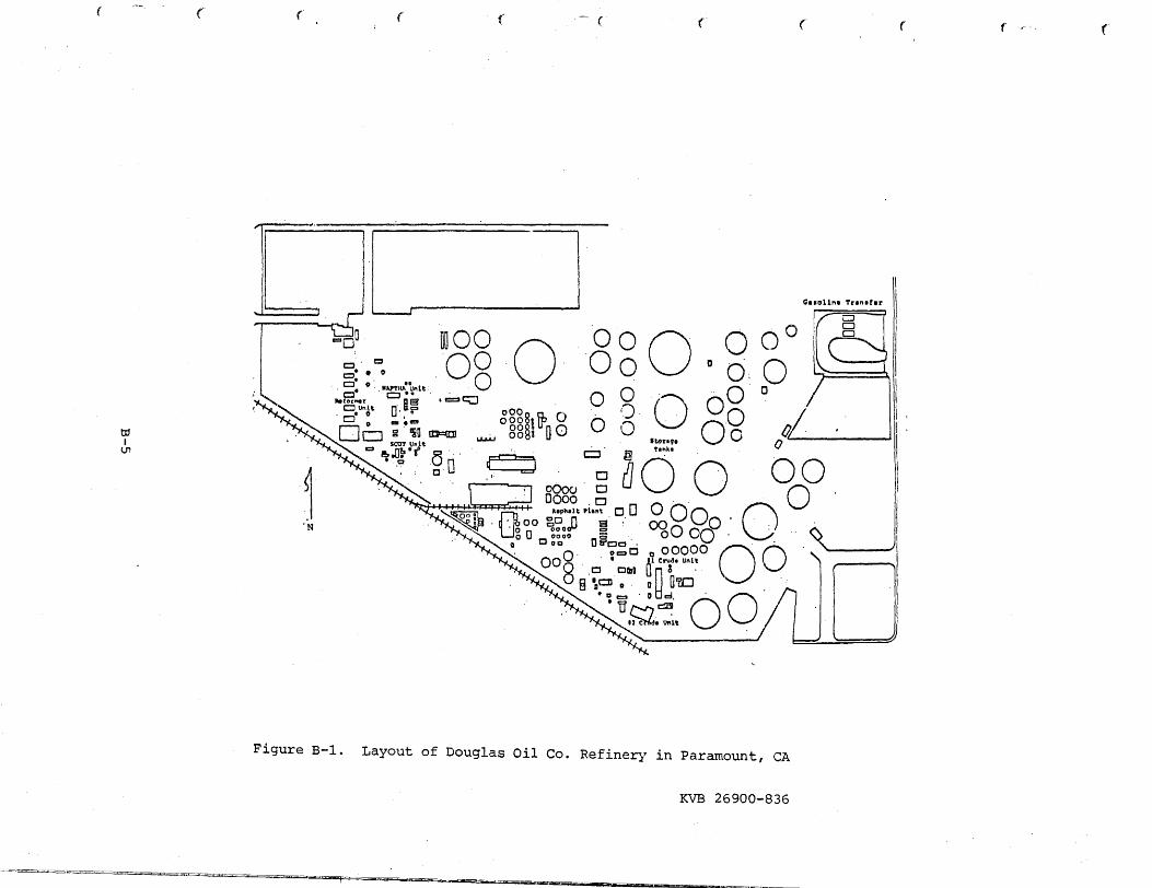
( ( ( ( { - ( ( ( ( ((- f

L I Ca,0Un• Tr ■n ■ rar

=~o" moo ·O _oo O o: •. o . oo . 0 0 :;. -~:·i·" . 0 .

D

Jlefo,... r

0

as ·=~ 0 0 . . .. c::J\llllt. a· II.co O 0· r::::::::l O ·, • oOO i

o :-·- ogg8dr. o - '.J . . tII D - ,iu D=mJ - 001<1 n O 0 O o· I D ~~t ~ ~ u

Cl e, .m, •r ,So:? . . . • . . . . lt.ortf ■u, • ,i;; U -=:1 - c::::J ~ T•~k•

. . c O a_ ::) . D 80 0-FD·.~ oo ._ :A _)?;.'.~ni.~ □. o o o·-0'

o_ oo . · 00 .0 0

O 0

Q Q 0

.N ~ 0,;__,~ 1Jn 00 ~~oJJ g 00 0 . . . o o

O 0000 :s _ 0 0 OQ . .

o oa Dli"oo .. ' ooO· :c=O a 00000 0 o·

8 ,,1 Crvd• U,,lt

.C Ctbt LJ ~ 3 . § 'aCD o · 0 Q'&J . '

·-:TI -o~. o· Q l~e\111°lt ·□

Figure B-1. Layout of Douglas Oil Co. Refinery in Paramount, CA

KVB 26900-836

Stack emissions were determined in the convential manner 1, except

that grab samples were also taken to per:mit speciation. Fugitive emissions

estimates were based on coarse leakage testing which results were expressed

as heav-y {0.15 cu. ft./min.), medium (0.025 cu. ft./min.) and small (0.002 cu.

ft./min.). The number of valves, flanges and pumps inventoriec2 for the

reformer unit, naphtha unit and the two crude units are shown in Table B-3.

This table also indicates the percentage of these components that were

tested on the program and the number of J.eakers, graded by size, found.

Where less than 100% of the components were tested, the number of leakers

found is extrapolated to the full population.

In the case of the testing of Douglas tankage, compositional data

only were acquired. Mass flows of emissions were calculated using AP-42

{thus the agreement for this category in Table B-2 for AP-42 and KVB data

columns). The assumptions used in rendering these calculations are as

follows:

Fixed Roof (API 2518)

Assumptions: Av. temp. 75op Point Factor 1.0 i",T=200F Tank Ullage = 1/3 Tank Height Tank Turnovers - Crude 35

Gasoline 10

Floating Roof (API 2517)

Assumptions: Av. temp .. 75°F 6 mph wind (4 mph at night) Welded, old, white

TABLE B-3. DOUGLAS OIL COMPANY VALVE, FLl~.NGE AND PUMP INVENTORY

Reformer Unit Na;ehtha Unit Crude Unit

Valves 500 {100%) 318 (100%) 475 (80%)

Heavy Leaks Medium Leaks Small Leaks

-0-26 13

-o---0-

5

2 9 7

Flan2es 852 (70%) 889 (70%) 1,319 (80%)

Heavy Leaks Medi um Leaks Small Leaks

-o-13

7

-o--o--o-

-o-7

11

Pumps 12 {100%} 7 (100%) 30 (100%)

Heavy Leaks Medi um Leaks Small Leaks

-0-1 1

-0--0--0-

l -o-

2

KVB 26900-836

B-6

APPENDIX C

ESTIMATION OF SOURCE STRENGTH USING REVERSE DIFFUSION CALCULATIONS

ETHYLENE DIBROMIDE EMITTED BY REFINERY GASOLINE TRANSFER AND LOADING OPERATIONS

KVB 26900-836C-1

In Section 3. 7. 5 .A of this report,1 ethylene dibromide (EDB) measure­

men ts at a refinery are discussed. These were made on an EPA-sponsored

study (Ref. 50) downwind of bulk transfer and tank truck loading operations.

The values obtained were 165 and 0.23 rng/m 3 at 50 and 400 ft., respectively,

from the designated centerpoint of the operations.

It was desired that these measurements be related to EDB release

rate at the source complex. The use of reverse diffusion calculations has

been employed before, although not always with notable success (Ref. 22-­

Appendix A). In any case, a very rough approximation would serve in making

comparisons with estimates derived by other approaches.

In the present case, the Gaussian distribution mod1el, modified by

Gifford ( Ref. 88) , was used. This is expressed as follows:

__Q~-·[1y2 2TIO 0 exp 2 (o ) ] · U -

y z y {exp [ - ½ ( ~ -H ) 2] + exp [ - ½ ( z ~ H ) 2) J

z z

Xis the concentration of the indicator substance at point x,y,z,

the coo'rdinates being relative to the ground level wind vector. Q is the

source strength or emission factor. His the effective plume height, which

includes source elevation. Wind speed is U and the O terms are vertical and

horizontal dispersion coefficients.

In the present exercise, assumptions were necessary since actual

conditions were not known. First, it was assumed that the measured values

were taken directly on the wind vector. Thus y = 0 and the first exponen­

tiated term of the equation becomes unity .. Sampling height (or z) was

asswned to be 2m and the wind speed 2. 24 m/sec. ( 5 mph) ..

The dispersion coefficients were taken from Reference 88, using

Class C stability category. This corresponds, at the given wind speed, to

daytime air stability with moderate solar radiation. The values would thus

be: ~

Station Dispersion Distance from Source Coefficients, m Feet Meters 0 0

z _x

40 15 1. 3 1.5 400 122 9 15

C-2 KVB 26900-836

The effective plume height was assumed to be 10 m. for the 400 ft.

station since there would be no propelling forces operating in the vertical

direction (as from conventional stacks) and the sources involved in the

present refinery analysis are largely close to the ground (tank trucks,

etc.). In the case of the close-in station at 50 ft., the plume height

was assumed to be 5 m. This derived from the assumption that the mean height

of the source complex was rather low and, since the station was so close in,

that vertical plume lift by any propelling effect would be small.

The Gifford equation was exercised using these variously estimated

values. The source strength (Q) results were 1.7 mg. EDB/sec. at 400 ft.

and 65 mg./sec. at 50 ft. The discrepancy, while not small, is consistent

with measurements that had been taken off the wind by the same angular

displacement. The closer in source would be more influenced by thisr

yielding larger values if they term is set at zero, as was done here.

C-3 KVB 26900-836

-~#############=#=#######################~

-~ ~ ~ ~ ~ ~ ~ ~ ~ ~

: AN INVENTORY OF CARCINOGENIC SUBSTANCES RELEASED : ~ INTO THE AMBIENT AIR OF CALIFORNIA ::ft:: ~ ::ft:: ~ ~

- ~ ~ ~ ~ ::ft:: TASK IV ~ ~ ~ ~ ~ ~ ~ ~ ~ ~ ~ ~ ~ ~ CONTRACT No. 1-068-32-221-12 ~ ~ ~ ~ ~ ~ ~ ~ ~ ~ ~ ~ ~ : PREPARED FOR :

~ SCIENCE APPLICATIONS, !NC, =it:: ~ ~ ~ Los ANGELES, CALIFORNIA - ~ ~ ~ ~ ~ ~ ~ ~ ~ ~ ~ ~ ~ ~ PREPARED BY ~ ~ ::ft:: ~ KVB., INC, ~

~ A RESEARCH-COTTRELL COMPANY ~ ~. ~.

~ ~

: ~

~ : ~ ,j

: A AelNrd\-Conrel C01111PMU 1:: ::ft::

~ MARCH 1980 ::ft:: ~ ::ft:: ~ '

-~ ~

~####################################:

;

'i.

,,_

CONTENTS

Section Page

1.0 INTRODUCTION 1

2.0 LABORATORY PROCEDURES 8

2.1 Arsenic Analysis 9 ._ 2.1.1 Current Methodology 9

2.1. 2 Analytical Problems 10

2.1. 3 Recom.~ended Approach 12

2.1.4 Laboratory Qualifications 13 ,._ 2.2 Asbestos Measurements 14

2.2.1 Current Methodology 14

2.2.2 Problems with the Methodology 15

2.2.3 Recommended Approach 18 .....,

I 2.2.4 Laboratory Qualifications 18 I

2.3 Benzene Analysis 20

2.3.1 Nature of the Methodology 20

2.3.2 Analytical Problems 22

2.3.3 Recommended Approach 22

2.3.4 Laboratory Qualifications 23

2.4 Cadmium Analysis 24

2.4.1 Nature of the Methodology 24 ,.,_

2.4.2 Recommended Approach 25

2.4.3 Laboratory Qualifications 25 I

2.5 Halocarbon Analysis 27

2.5.1 Nature of the Methodology 27 ,._,

2.5.2 Analytical Problems 27

2.5.3 Recommended Approach 28

2.5.4 Laboratory Qualifications 28

,..,.

ii KVB 26900-836

Section

2.6 Nitrosamine Analysis 29

2.6.1 Nature of the Methodology 29

2.6.2 Analytical Drawbacks 30

2.6.3 Recommended Approach 30

2.6.4 Laboratory Qualifications 30

2.7 Polycyclic Organic Matter (POM) Analysis 32

2.7.1 Nature of the Methodology 32

2.7.2 Analytical Problems 33

2.7.3 Recommended Approach 34

2.7.4 Laboratory Qualifications 34

2.8 Quality Assurance - Laboratory 35

3.0 TEST PLAN 37

3 .. 1 Stationary Source Testing 37

3.1.1 Primary Steel Mill 38

3 .. 1.2 Refinery Operations 55 .....

I3.1.3 Carbon Tetrachloride/Perch1oroethylene 64 Manufacturing Plant

3.1.4 Carbon Tetrachloride Conversion Plant 69

3.1.5 Ethylene Dichloride Production Plant 73

3 .1 .. 6 Secondary Lead Smelter 77

3.1.7 Asbestos Mining and Milling Operations 80

3.1.8 Power Plants 83

3.1.9 Asbestos Consuming Plants 84

3.2 Special Testing 88

REFERENCES 90

APPENDIX:

A. BAT'rELLE COLUMBUS LABORATORIES METHOD FOR PAH ANALYSIS A-1

iii KVB 26900-836

......

FIGURES

Number

3-1 Typical iron ore sinte:ring process 45

3-2 Kaiser steel mill: of plant

General plan of northeast portion 48

3-3 Location of Dow Chemical Company CT/Pere Plant in Pittsburg

67

.......

iv KVB 26900-836

TABLES

Number Page ......

1-1 Eleven Suspected Carcinogenic Substances Selected for 2 Specific Study in Task II

1-2 Summary of "Hot Spots" Identified in Ta.sk II and Their 3 Relative Scaling Using an Arbitrary Hazard Formula

1-3 Categories of Stationary Sources Considered in the Test Plan 5

2--1 Results of TEM-SAED Chrysotile Counting. in EPA-Sponsored 16 Round Robin

3-1 Target Pollutants Associated with Steel Mill Operations 39

3-2 Computed Kaiser Steel Corp. Coke Oven Fugitive Emissions 42 Using Current SCAQMD Emission Fee Factors

3-3 Volatile Organic Stack Gas Emissions from Under-Fired 44 Coke Ovens

3-4 Summary of Pollutant ':r'esting Operations Proposed for the 54 Kaiser Steel Plant, Fontana

3-5 Percentage Frequency uf Wind Direction and Speed 66

3-6 Analysis of Asbestos Fiber Emissions 86

3-7 Special Testing of Nonstationary Sources Suggested by 89 Program Findings

V KVB 26900-836

SECTION LO

INTRODUCTION

- The development of an inventory of carcinogenic substanc~s released

into the ambient air of California involved a four-element program, the last

of which, Task IV 6 is described in this volume. The overall organization of

these tasks is as follows:

TASK I (SAI) - Identify a limited number of carcinogens posing the

greatest potential hazard as ambient atmospheric pollutants in California.

TASK II (KVB) -- Locate major sources of and estimate emission factors

for this list of carcinogens.

TASK III (SAI) - Determine usage patterns, release rates, and popula­

tion exposures for the sixteen substances regulated by the Occupational

Carcinogens Control Act and investigate substances of concern by incorporating

them into the Task I evaluation.

TASK IV (KVB) - Develop a field test plan to verify the more significant

factors· estimated on Task II.

As discussed in the Task I volume, 114 substances regarded by the EPA

as having carcinogenic potential were screened. By rating these under the

criteria of: (1) annual U.S. production; (2) fraction lost during production;

(3) volatility; and (4) carcinogenicity, the group was reduced to 35 substances

(compounds or classes of compounds). Further reduction of the list was done

through semi-objective quantitative algorithms based upon adding and multiply­

ing rating factors. These included all the factors listed above (except as

applied to the State rather than National level) plus rating factors for:

(1) projected growth in usage; {2) stability in ambient air; and (3) potential

for dispersion after release. Application of this refinement resulted in a

ranked list of 22 substances.

1 KVB 26900-836

The selection process further involved a review by an ad hoc panel of

experienced scientists convened by SAI. From this and two final .-1-,•-listings,1/,•1

the eleven highest scoring substances wer,e then selected for study in Task II.

These are listed, alphabetically, in Table 1-1.

TABLE 1-1. ELEVEN SUSPECTED CARCINOGENIC SUBSTANCES SELECTED FOR SPECIFIC STUDY IN TASK II

Arsenic Ethylene dibrornide

Asbestos Ethylene dichloride

Benzene Nitrosamines

Cadmium Perchloroethylene

Carbon tetrachloride Polycyclic Organic

Chloroform Matter (POM}

On the Task II effort 1 which is discussed in another volume of this

report, sources were identifi-ed where the highest concentrations of emissions

of these substances were suspected. This was based on the analysis of

published data, together with contacts 11.,;rith qov8rnment agencies and major

producers and/or users of these m2.terials. Stationary sources, recognized

as "hot spots," t.1ere then displayed on maps 1, whenever practical, and coded

according to the ranges of estimated quantities released per unit of time.

A number of the pollutants studied were associated with area or dispersed

sources. These would thus not emerge as 11 hot spots,n although comparatively

large total releases were involved in some cases.

So that "hot spots 11 identified could be roughly graded or prioritized

for source testing planning, an arbitrary scaling factor was applied. This

was arrived at in a manner similar to that used in Task I for the comparison

of suspected carcinogens with one another with respect to hazard potential.

The application of this formula resulted in the listing of seventeen 11 hot spots 11

that are detailed in Table 2-1 of the Task II report. An abbreviated version

of that tabulation is presented here as Table 1-2.

2 KVB 26900-836

--

( ( (( ( ( ( ( --{ ( ( ,,,...=-::-.,,_

TABLE 1-2 . SUMMARY OF uHOT SPOTS II IDENTIFIED IN TASK II AND THEIR RELATIVE

SCALING USING AN ARBITRARY HAZARD FORMULA

Estimated Scaling -6

Site Pollutant Emissions, tpy Factor x 10

Kaiser Steel Corp., Fontana

Stauffer Chemical, Carson

Dow Chemical USA, Pittsburg w

DuPont de Nemours & Co., Antioch

Chevron USA, Richmond

ARCO, Carson

Allied Chemical, El Segundo

~ Witco Chemical Co., Carson Iv C' I.D Chevron USA, El Segundo 0 0 I Gould Inc., Vernon

co w C' RSR Corp., Industry

Benzene

Cadmium

Arsenic

POM

Ethylene dichloride

Carbon tetrachloride

Perchloro-ethylene

Carbon tetrachloride

Benzene

Benzene

Carbon tetrachloride

Benzene

Benzene

Arsenic

Arsenic

112

7.0

1.6

27 *

Total

150 i'

160 §

22 §

Total

250 #

50

25

113 #

14

30

22

3.3

54.5

3.4

0.5

17.5

75.9

55.2

41.8

5.7

47.5

41.8

35.0

21.1

17.8

14.0

12.0

3.5

1.3

TABLE 1-2. (Continued)

Site Pollutant

ALCO-Pacific, Carson Arsenic

Pacific Gas & Elec., Arsenic

Johns-Manville, Stockton Asbestos

Calavaras Asbestos, Copperopolis Asbestos

So. Cal. Edison, Long Beach Arsenic

Pacific Gas & Elec., Salinas Arsenic

Estimated Scaling Emissions, tpy Factor x 10-6

2.2 1.3

1.0 0.4

2.9 0.3

148 0.3

0.8 0.3

1.0 0.02

Notes:

* Assumes POM/benzo(a)pyrene (BaP) = 10; BaP actually measured

t A minimum estimate ~

§ Process factors suggest that the large difference between CT and perc emissions is suspect (See Sec. 3.5.2

#Maybe high by

~ N O'I w 0 0 I

a:> w (j\

(A))

an order of magnitude

j ) ) j ) ) )

-

The Task III effort aimed at expanding the scope of Task I to

include sixteen cancer-causing substances regulated by the State under the

Occupational Carcinogens Control Act.

These substances were studied in the same manner as the target com­

pounds considered in Task I. Those materials found to be high scoring on

being tested with the screening- algorithms were then input into Task I for

comparative evaluation with the materials of interest in that task that had

already been similarly screened. Thus Task III actually represented an

expansion of scope of the Task I work. The output of the latter included

input target materials for both tasks and became the common focal point for

the Task II studies.

The objective of Task IV, which .is the topic of the present discussion,

was to develop a plan for a source-testing program which, if implemented, would

verify or correct the emission factors estimated for the top seventeen "hot

spots" in California. The initial requirement was to determine if access to

the various plants would be permitted such that at least one site representative

of each plant or process type category would be accessible. These categories

are listed below. Three of the eleven topical cnrcinogens are seen not to have

been identified as pollutants for anv of the seventeen "hot spots."

TABLE 1-3. CATEGORIES OF STATIONARY SOURCES CONSIDERED IN THE TEST PLAN

Number Listed Plant Category or Subprocess_ on Table 1- 2 Pollutant (s)

Integrated Steel Mill 1 Benzene Cadmium Arsenic POM

EDC-Synthesis 1 EDC

Carbon tetrachloride perc synthesis

(CT)/ 1 CT & perc

Carbon tetrachloride converters 2 CT

Benzene synt},zsis/conv·~rsion and/or gasoline refining 4 Benzene

secondary lead smelter 3 Arsenic

Oil-fired power plant 3 Arsenic

Asbestos-contai~ing product manufacture 1 Asbestos

Asbestos mining 1 Asbestos

5 KVB 26900-836

1,1 I

With the exception of utility companies and one benzene consumer

(Chevron-USA, Richmond) , all of these plants wer•e contacted. Omission of

contact with the utilities was prompted because power plant access was believed

to be readily forthcoming and the sites so familiar as to obviate the need

for inspection. Chevron-USA, El Segundo, was contacted in preference to the

Richmond plant because it represented a more interesting test site (see Sec.

3 .1. 2 .A) . It is the only refinery in the State that both rnanuf.:...ctures and

consumes benzene.

With one exception, access to a t,est site within each category was

extended, but usually with the provision that the test plan was found to be

technically acceptable by the intended host. The one exception was the Dow

Chemical plant at Pittsburg; emission factor estimation using the Virtual

Source Test Method will thus be required there.· In the case of the other

categories and where more than a single plant offered access, the best

candidates were identified using Task II information. Site visits were then

arranged and conducted at most of the "open'' plants. Because of the informa­

tion supplied and the nature of the test work contemplated (see Sec. 3.1.7

and 3.1.9), visits to the asbestos mine and the asbestos/cement pipe works

were considered unnecessary.

As a result of the site visits, considerable proprietary information

was acquired. In most cases, secrecy or proprietary information agreements

were stipulated. It was also required that the preliminary test plan developed

for these plants be reviewed for content by the host companies. The present

discussions, therefore, avoid process details that are regarded as proprietary

by these companies.

Using the information thus gained, a general test approach was next

developed for each host plant and submitted for review, where required. Some,

but not all, of the comments received back have been incorporated in the

present volume.

6 KVB 26900-836

-

'-

Additionally, methodology for the overall pertinent analytical chemistry

and asbestos counting is examined and optimum techniques recommended. This

proved particularly appropriate since measurement of several of the analytes*

(arsenic, asbestos and POM) is by no means routinized and/or ruggedized~t

Another section of this volume deals with nonstationary sources which,

though not "hot spots," account for releases of significant amounts of

materials from dispersed or area sources. This section is called "Special

Testing". It briefly itemizes the identified problems and suggests the

general type of testing that would be appropriate for each source type.

Section 2.0, which next follows, deals with chemical analytical and

oth~r measurement methodology. This is presented first, so that the

selection of modalities of sampling for these analytes that is discussed in

the test plan will be better appreciated. Section 3.0 presents a discussion

of the test approaches recommended for the various plant categories. This is

followed by a subsection on "Special Testing."

,........

* 11 Analyte 11 is a term generally used by analytical chemists to describe the thing that is measured by a chemical analytical procedure.

t "Ruggedization" is a term widely used by analytical chemists, particularly in government agencies (EPA, NIOSH, FDA etc.). The term denotes the exercise of an analytical method to the degree adequate to determine its precision and ·accuracy, and its sensitivity to chemical or other interferences.

7 KVB 26900-836

SECTION 2.0

LABORATORY PROCEDURES

In the following subsections, the methodology applied in environmental

test laboratories for the measurement of the eleven materials of interest is

reviewed. Procedures are favored which would furnish adequate sensitivities

for trace substances having potentially potent pathogenic properties and which

are reasonably available and relatively economic to employ. These include

techniques in some degree of use at the EPA, NIOSH, OSHA and other agency

laboratories, as well as contractor labs under contract to these agencies.

While the detection limits of the various techniques are discussed

in either specific or general terms, the sample size requirements are not.

This will be determined by a number of factors, the consideration of which

would involve detailing beyond the scope of this study. As a generalization,

however, the sample sizing should conform with the formula:

Where:

V = Sample volume (vapor equivalent)s

M = Detectable mass0

c = Concentration of analyte in V s

a = Aliquoting factor (fraction of analyte in V actually seen by the detector) s

This rule of thumb thus specifies a sample volume that will provide to the

detector an analyte mass that is five times, at least, the detection limit of the

detector. As will be pointed out, detection limits are not always accurate

values, and measurements at levels well below these limits are frequently

reported without comment on that fact.

8 KVB 26900-836

2.1 ARSENIC ANALYSIS

2 .1.1 Current Methodology

The techniques in most prevalent usage for environmental arsenic

analysis are colo.rimetric r atomic absorption spectroscopy (AAS) , and vol tam­

metry. All require wet ashing of the sample filters, usually with a combina­

tion of nitric, perchloric and sulfuric acids. Aside from low temperature

ashing in a microwave furnace (Ref. 1), the use of elevated temperature

ashings or fusions of arsenic-containing samples are avoided because of the

comparatively high volatility of the metal and its salts.

The colorimetric procedure is cornrnonly used and is recommended by

EPA (Ref. 2), the NIOSH {Ref .. 3), the American Conference of Governmental

Industrial Hygienists (ACGIH) (Ref. 4), and the Association of Official

Agricultural Chemists (AOAC) (Ref. 5). The solubilized arsenic is converted

to arsine with a hydrogen sm.irce (NaBH ) {Ref. 6) or the classical Zn/HCl4

mixture and collected in a pyridine solution containing silver diethyldithio-

carbamate. Arsine reacts with the latter to form a colored adduct which is

photometrically measured at 560 nm. The detection limit would be about

0. 2 ]Jg/:i:-,.3 in air, assuming 60 cu ft is passed through the filter. Use of the

method for lead smelter effluents is contraindicated since antimony, a sig­

nificant constituent in the input scrapr interferes.

Of the A.A,S techniques, three versions can be employed: (1) direct

solution aspiration into the flame; (2) direct hydride aspiration into the

flame; and (3) graphite furnace solution injection. Method {l) is not favored

for trace-rea1m work because detectivity* is not impressive (>l l-lg/m3 - 60 cu ft

sample) and accuracy is often compromised by matrix effects (Ref. 7)~ The

hydride/flame AAS technique is more sensitive. Absence of solvent enhances

ana.lyte ionizability and, thus, specific responses. Typically a detection 3

lirni t of less than 50 ng/rn (60 cu ft sample) is obtained {Ref. 7) .. The

MS graphite furnace furnishes a sensitivity of about that of the AAS hydride

technique (Ref. 7). It is specified for use by the NIOSH (Ref. 3) and the

EPA (Ref. 8).

·* "Detectivity" is the.term specified by the 1\merican Chemical Society to denote the limit of detection of a measurement, usually assuming a signal to noise ratio of 5:1.

KVB 26900-836 9

Another technique that has received Government acceptance (Ref. 3)

is the voltarnrnetric approach. After conventional wet ashing, pentavalent

arsenic is reduced to As(III) with NaHS0 /Fe(Cl0 ) • The Fe(II) is stabilized3 4 2

by addition of hydrazine and As(III) determined by anodic stripping, using a

composite gold-graphite electrode. The detection limit of the procedure is

about the same as for the graphite furnace and hydride AAS procedures.

Bismuth and antimony interfere but can be corrected for if separately

determined.

Another technique that has been adopted by the NIOSH (Ref. 3)

involves the measurement of iodide oxidation (by bromate) as controlled by

osmium catalysis (Ref. 9--12). Arsenic promotes the catalysis such that

iodine concentration is proportional to As (III)· level. The former is determined

colorimetrically. The detection limit is about 2 ng/m3 {60 cu ft sample);- copper (II) and ammonium ions interfere.

Neutron activation analysis (NAA) has been employed to achieve low

detection limit quantitative analysis of arsenic (Ref. 13). Although

applied to direct analysis of oil samples, measurement of arsenic in conven­

tionally digested air-filter samples should furnish a lower working limit of 3

about 5 ng/m by the cited NAA approach.

A number of other techniques can be employed for arsenic analysis.

These include such approaches as mass spectrometry (spark source and

secondary ionization), emission spectroscopy (flame, arc and inductively

coupled argon plasma modes), X-ray fluorescence spectroscopy, polarography,

various micro-field spectroscopic techniques (Auger, microprobe, X-ray

energy dispersive, ESCA), and so on. Due to limitations in the individual

cases, these methods are not widely used for the quantitative analysis of

arsenic on filters.

2. 1.2 Analytical Problems

Either the graphite furnace or hydride AAS analysis would appear to

be an.acceptable approach for arsenic analysis. Neither is known to be

susceptible to :matrix or other interferences (Ref. 3); both are widely

10 KVB 26900-836

practiced, offer adequate sensitivity for source-acquired filter samples,

and are endorsed by the EPA and the NIOSH.

Robbins et al of Asarco have published (Ref. 14) round robin

results that show acceptable precision but poor accuracy in arsenic analyses 3

at levels equivalent to 4.3 and 6.B µg/rn (60 cu ft sample). The methods

employed (ad lib) included the arsine AAS 1, vol tarnmetry and colorimetric

procedures.

The State's Air and Industrial Hygiene Laboratory (AIHL) verified

the problem using the graphite furnace AAS approach {NIOSH Method S309).

AIHL's Lew stated (Ref. 14) that the poor recovery of 53-61% for the lower

and 58-68% for the higher concentration samples obtained by S309 agreed

reasonably well with Robbins' x·ound robin results of 62% and 71%, respec­

tively. Lew concluded that NIOSH method S309 would be inappropriate for the 3

current arsenic standard of lOµg /m .

When contacted, Lew suggested that because of the low concentration

involved, a more sensitive technique,, such as voltammetry, would be

appropriate. This did not prove convincing, since the voltammetric approach

had been employed (with recov,eries of 81% and 64% for the two levels cited

above) on the Robbins round robin. Also, the arsenic levels were at least

two orders of magnitude above the graphi t,e furnace .AAS detection lirnit.

It would appear that the problem is not inherent in the various

measurement techniques employed, all of which should have been adequately

sensitive, but in the sample preparation. .All of the methods involve digestion

of the filters under fuming perchloric acid conditions. Such an elevated

temperature promotes arsenic volatilization. This is why NIOSH method S309

requires the application of a recovery factor, which is developed

(independent of the usual calibration curve preparation) using standards that

are carried through the complete procedure. It is not clear that this was

done in either the Robbins or the CALOSHA studies. Even if applied, however,

the recovery factor use is problematic in that it varies with concentration.

The overall problem has been recognized by the OSHA Analytical

Laboratory in Salt Lake City. There, the digestion step involves only the

11 KVB 26900-836

use of nitric acid. Unlike the colorimetric, voltarnrnetric, or hydride AAS

methods, nitric acid is compatible with the graphite furnace AAS procedure.

Solubilization of arsenic in nitric acid is excellent. The filter is also

completely dissolved, if not completely digested (to co ).2

Arsenic volatilization is supressed by the addition of Ni(N0 ) 2

.3

Based on the results at OSHA, Salt Lake, this technique is effective when

nitric acid digestion is involved. CALOSHA found it ineffectual at the

higher temperature perchloric acid digestion conditions.

Arsenic recoveries at OSHA, Salt Lake, typically exceed 90% when

working in the range considered by Robbins. Although not published in the

open literature, the procedure is available on request and is recommended

for the present requirement.

The analytical chemists at OSHA who supplied the above comments

(L. Larson and J. Septon) also noted the work done by D. V. Sweet at NIOSH,

Cincinnati. In lieu of the S309 perchloric/nitric acid digestion, that

worker dry-ashed her filters in a microwave low-temperature asher. She

worked with as little as 30 ng As/filter, which borders on detection limit,

but experienced an average arsenic recovery of 101% using a graphite

furnace AAS finish. Nickel spiking was not employed.

Sweet presented her results recently (Ref. 15) and the method will

be incorporated in the NIOSH Manual of Analytical Methods as P & CAM No. 286.

At present, the method is unclassified but will be designated as either

Class D (operational) or Class E (proposed). Negotiations are currently

underway to retain a contractor who will ruggedize the procedure, that is,

fully exercise the procedure against interferants, over the full working

range and with equipment variables. If successfully emergent (variance

analysis demonstrates acceptable precision and accuracy), the method will

be given a Class B (accepted by NIOSH) designation.

2.L 3 Recommended Approach

The OSHA, Salt Lake City, graphite furnace AAS procedure_is

recomrne:nded. The NIOSH P & CAM No. 286 procedure will also be endorsed

if proved acceptably rugged in upcoming testing.

12 KVB 26900-836

The EP.~ is currently developing a reference method for the sampling

and analysis of arsenic in flue gases. 1,,7hile the former portion was com­

plete and appeared satisfactory, the analytical methodology was still not

set. Thus, no comment on this agency 1 s procedure can be offered at this time.

2. 1. 4 Laboratory Qualifications

Assuming that an adequate QA program is effectively in place (see

Sec. 2. 8), any laboratory offering the requisite AAS equipment should be

capable of performing the arsenic measurements. The AA spectrophotometer

should have a monochromator with a reciprocal linear dispersion of about

0.65 nm/mm in the u.v. region. "rhe use of a background corrector is abso­

lutely necessary in order to avoid molecular sc.attering effects at the working

wavelength (193. 7 nm). An electrodeless arsenic lamp should be used. A

direct readout (metric or recorder) proportional to absorbance W1its should

be provided.

If the P & CJlu1 Method 286 is employed, a suitable low temperature

ashing system will be required. The International Plasma Model PM 1604 has

furnished satisfactory results in NIOSH tests.

13 KVB 26900-836