New Longitudinal Error Balancing Approaches for Closed ...
109
Georgia Southern University Digital Commons@Georgia Southern Electronic Theses and Dissertations Graduate Studies, Jack N. Averitt College of Summer 2021 New Longitudinal Error Balancing Approaches for Closed Traverses Jose L. Manzano Follow this and additional works at: https://digitalcommons.georgiasouthern.edu/etd Part of the Civil Engineering Commons, and the Construction Engineering and Management Commons Recommended Citation Manzano, Jose L., "New Longitudinal Error Balancing Approaches for Closed Traverses" (2021). Electronic Theses and Dissertations. 2295. https://digitalcommons.georgiasouthern.edu/etd/2295 This thesis (open access) is brought to you for free and open access by the Graduate Studies, Jack N. Averitt College of at Digital Commons@Georgia Southern. It has been accepted for inclusion in Electronic Theses and Dissertations by an authorized administrator of Digital Commons@Georgia Southern. For more information, please contact [email protected].
-
Upload
khangminh22 -
Category
Documents
-
view
2 -
download
0
Transcript of New Longitudinal Error Balancing Approaches for Closed ...

Georgia Southern University
Digital Commons@Georgia Southern
Electronic Theses and Dissertations Graduate Studies, Jack N. Averitt College of
Summer 2021
New Longitudinal Error Balancing Approaches for Closed Traverses Jose L. Manzano
Follow this and additional works at: https://digitalcommons.georgiasouthern.edu/etd
Part of the Civil Engineering Commons, and the Construction Engineering and Management Commons
Recommended Citation Manzano, Jose L., "New Longitudinal Error Balancing Approaches for Closed Traverses" (2021). Electronic Theses and Dissertations. 2295. https://digitalcommons.georgiasouthern.edu/etd/2295
This thesis (open access) is brought to you for free and open access by the Graduate Studies, Jack N. Averitt College of at Digital Commons@Georgia Southern. It has been accepted for inclusion in Electronic Theses and Dissertations by an authorized administrator of Digital Commons@Georgia Southern. For more information, please contact [email protected].

NEW LONGITUDINAL ERROR BALANCING APPROACHES FOR CLOSED TRAVERSES
by
JOSE LIWENG MANZANO
(Under the Direction of Gustavo Maldonado)
ABSTRACT
This study presents two novel approaches to balance the horizontal longitudinal error of closure,
EC, in closed polygonal traverses. The standard procedure to balance EC is the Compass Rule.
This technique reduces EC to zero by applying corrections in the lengths of all traverse sides.
Those corrections are proportional to the corresponding side lengths. That is, this approach is not
an error-correcting approach, but an error-balancing procedure. The proposed new techniques
are based on sensitivity analysis of EC with respect to small variations, Δi, in the lengths of all
sides i = 1, 2, …, n of the traverse, where n is the total number of sides. In fact, for improved
visualization purposes, the sensitivity analysis is performed on quantity D = P/EC, where P is the
perimeter of the traverse. Additionally, D is the denominator of the Longitudinal Precision Ratio,
LPR = 1/D, of the traverse. The presented new schemes first select the side lengths to be
modified as those showing the most pronounced variations in D. Then, after the length of a few
selected sides are modified, the Compass Rule is applied to close the remaining small gap. One
of the proposed schemes requires a single sensitivity analysis and modifies the length of a few
sides simultaneously, whereas the other scheme requires iterative sensitivity analyses and
modifies the length of only one side per iteration. Potential weaknesses of the

proposed schemes were investigated and analyzed. Additionally, an attempt was made to
corroborate if the proposed schemes were truly error-correcting approaches or just error-
balancing ones. However, the attempt was inconclusive due to unexpected inaccuracies in a few
side lengths employed as benchmarks. Those lengths were obtained from vertex coordinates
acquired by Leica GS14 antennas. Unfortunately, 2 vertices out of 7 presented quality-control
parameters slightly out of the suggested preferred ranges. Therefore, it could not be concluded
that the proposed schemes are truly error-correcting ones. Nevertheless, they effectively reduce
and fully eliminate the horizontal longitudinal error of closure in closed polygonal traverses.
This corroborates that they are, at least, new effective error-balancing procedures.
INDEX WORDS: Closed traverse, Surveying, Compass rule, Bowditch rule, Error of closure,
Sensitivity analysis

NEW LONGITUDINAL ERROR BALANCING APPROACHES FOR CLOSED TRAVERSES
by
LIWENG MANZANO
B.S., Georgia Southern University, 2019
A Thesis Submitted to the Graduate Faculty of Georgia Southern University
In Partial Fulfillment of the Requirements for the degree
MASTER OF SCIENCE

©2021
LIWENG MANZANO
All Rights Reserved

1
NEW LONGITUDINAL ERROR BALANCING APPROACHES FOR CLOSED TRAVERSES
by
LIWENG MANZANO
Major Professor: Gustavo Maldonado
Committee: Marcel Maghiar
Francisco Cubas-Suazo
Electronic Version Approved:
July 2021

2
ACKNOWLEDGMENTS
I gratefully acknowledge the assistance of undergraduate students including Keith
Stevens, Wesley Duncan, John Williams-Rosario, Colby Polk, Sierra Lackey, Ryan Wren, Shay
Stripling, Teresa J. Vazquez, and graduate students Ananya Augustine and Mariah Peart. I would
also like to express my gratitude for the hard work and contributions of my advisor Dr. Gustavo
Maldonado leading to the successful completion of this project. I also extend my gratitude to my
committee, Dr. Francisco Cubas Suazo and Dr. Marcel Maghiar, for guiding me through the
finalization of this project.

3
TABLE OF CONTENTS
Page
ACKNOWLEDGMENTS …………………………………….......................................................... 2
LIST OF TABLES.............................................................................................................................. 4
LIST OF FIGURES ............................................................................................................................ 5
CHAPTER
1 INTRODUCTION …………………………..…………………………………………… 6
2 PREVIOUS STUDIES ………………………..………………………………...……..… 11
3 EMPLOYED INSTRUMENTS ……………….………………………………….……... 13
4 METHODOLOGY ……..………………………………………………………….……. 18
Field Procedure …………………………………………………………………… 18
Data Processing …………………………………………………………..……… 18
Compass Rule …………………………………………………………….……… 22
Proposed Procedure to Balance the Longitudinal Error of Closure ……………... 24
OPUS/GPS Procedure ………………………………………………………….... 31
5 RESULTS …………………………………………………………………………….… 35
Case Study one: El Sombrero ................................................................................. 35
Case Study Two: El Sombrero ................................................................................ 36
Case Study Three: Georgia Southern University- Statesboro ……………………. 43
Successive-Sensitivity Application of the Proposed Balancing Method ...………. 51
Comparison of Proposed Approach against GNSS-Collected Data …………....… 55
Analysis of Results ………………………………………………………..…..….. 59
Virtual Case: Rectangular Traverse .……………………………………….……... 62
6 CONCLUDING REMARKS ………………………………………………...………….. 67
Potential Improvements to be Considered……………………………...………… 71
Further Studies ………………………………………………………...………….. 72
REFERENCES ................................................................................................................................... 74
APPENDICES .................................................................................................................................... 75
A Protocol to Perform Static-GPS with GS14 …………………...…………………….. 75
B Point Acquisition for Closed Traverse with Azimuth Protocol ...………………….... 81
C A New Longitudinal Error Balancing Approach for
Closed Traverses - Mathematical Model ………………………...……………..…… 91
D Opus Emails for Points 1-7…………………………………………………………… 97

4
LIST OF TABLES
TABLE
3.1 Leica Viva GS14 Specifications…………………………………………………………14
3.2 One-second Robotic Total Station Specifications……………………………………….15
3.3 GPT-3200NW Series Specification……………………………………………….……..17
4.1 Case Study 1 (7-sec instrument) - Internal Angle at Vertex T1 …………………….....19
4.2 Case Study 1(7-second instrument) – Overall Angular Error Balancing……………....20
4.3 Case Study 1 - Case Study 1(7-sec instrument) – Azimuths of Each Side…………......21
4.4 Case Study 1 (7-sec instrument)- Longitudinal Balancing via Compass Rule ………...23
4.5 Case Study 1 (1-sec instrument)- Overall Angular Error Balancing…………………...24
4.6 Case Study 1 (1-sec instrument)- Longitudinal Balancing via Compass Rule ……..….25
4.7 Case Study 1 (1-sec instrument)- Sensitivty of Pseudo Longitudinal Precision Ratio....26
4.8 Case Study 1 (1-sec instrument)- Longitudinal Balancing via the Proposed approach...29
4.9 Case Study 1 (1-sec instrument)- Vertex Coordinates after New Balancing Approach..30
5.1 Case Study 2 (1-sec instrument)- Overall Angular Error Balancing…………………...38
5.2 Case Study 2 (1-sec instrument)- Longitudinal Balancing via Compass Rule…………38
5.3 Case Study 2 (1-sec instrument)- Sensitivity of Pseudo Longitudinal Precision Ratio...39
5.4 Case Study 2 (1-sec instrument)- Longitudinal Balancing via the Proposed approach...42
5.5 Case Study 2 (1-sec instrument)- Vertex Coordinates after New Balancing Approach..42
5.6 Case Study 3 (1-sec instrument)- Overall Angular Error Balancing…………………...44
5.7 Case Study 3 (1-sec instrument)- Longitudinal Balancing via Compass Rule…………45
5.8 Case Study 3 (1-sec instrument)- Sensitivity of Pseudo Longitudinal Precision Ratio...46
5.9 Case Study 3 (1-sec instr.)- Longitudinal Balancing via the Proposed approach............50
5.10 Case Study 3 (1-sec instr.)- Vertex Coordinates after New Balancing Approach……...51
5.11 First Iteration of the Successive-Sensitivity Alternative Approach…………………….52
5.12 Second Iteration of the Successive-Sensitivity Alternative Approach…………………53
5.13 Third Iteration of the Successive-Sensitivity Alternative Approach…………………...54
5.14 Vertex Coordinates after the 1st, 2nd, and 3rd iteration………………………………….54
5.15 Received OPUS Coordinate Data for all Seven Vertices of Case Study 3……………..55
5.16 Additional Data from OPUS……………………………………………………………56
5.17 Vertex Coordinates, Side Lengths and Perimeters from 5 Different Approaches……...57
5.18 Discrepancies in Horizontal Lengths with Respect to GNSS-Measured Lengths……...58
5.19 Virtual Rectangular Traverse – Error Balancing Via Compass Rule..….…………….. 63
5.20 Virtual Rectangular Traverse – Final Vertex Coordinates Via Compass Rule….…….64
5.21 Virtual Rectangular Traverse – Error Balancing Via Proposed Simultaneous Scheme..66

5
LIST OF FIGURES
FIGURE
1.1 Case Studies 1 (North) and 2 (South) Traverses at El Sombrero Restaurant Site……8
1.2 Case Study 3 Georgia Southern University Statesboro Campus Traverse..........…….9
3.1 Leica GRZ122 360° Prism………………………………………………....……….13
3.2 Leica Viva GS14……………………………………………………………...…….13
3.3 One-Second Leica TRCP 1201+ Robotic Total-Station Instrument………………..14
3.4 Leica CS10 Controller……………………………………………………………....16
3.5 Seven Second GPT-3200NW Total-Station Instrument……………………………19
4.1 Latitude and Departure Components of a Traverse Side…………………….……..21
4.2 Sensitivity of Pseudo Longitudinal Precision with Respect to Distance T1-T2…....27
4.3 Sensitivity of Pseudo Longitudinal Precision with Respect to Distance T2-T9……27
4.4 Sensitivity of Pseudo Longitudinal Precision with Respect to Distance T9-T6……28
4.5 Sensitivity of Pseudo Longitudinal Precision with Respect to Distance T6-T1……28
4.6 Error Convergence for OPUS Horizontal Coordinates (from OPUS website)……..31
4.7 Sample OPUS Online Screen to Submit Captured GNSS Data……………………33
5.1 Case Study 1: El Sombrero Restaurant- North Traverse………………………...…35
5.2 Case Study 2: El Sombrero Restaurant- South Traverse………………………...…37
5.3 Sensitivity of Pseudo Longitudinal Precision with Respect to Distance T1-T12…..40
5.4 Sensitivity of Pseudo Longitudinal Precision with Respect to Distance T12-T15…40
5.5 Sensitivity of Pseudo Longitudinal Precision with Respect to Distance T15-T16....41
5.6 Sensitivity of Pseudo Longitudinal Precision with Respect to Distance T16-T01…41
5.7 Case Study 3: Seven-sided Traverse at Statesboro Campus………………………..43
5.8 Sensitivity of Pseudo Longitudinal Precision with Respect to Distance 1-2……….46
5.9 Sensitivity of Pseudo Longitudinal Precision with Respect to Distance 2-3……….47
5.10 Sensitivity of Pseudo Longitudinal Precision with Respect to Distance 3-4……….47
5.11 Sensitivity of Pseudo Longitudinal Precision with Respect to Distance 4-5……….48
5.12 Sensitivity of Pseudo Longitudinal Precision with Respect to Distance 5-6……….48
5.13 Sensitivity of Pseudo Longitudinal Precision with Respect to Distance 6-7……….49
5.14 Sensitivity of Pseudo Longitudinal Precision with Respect to Distance 7-1……….49
5.15 Discrepancies in Horizontal Lengths with Respect to GNSS-Attained Lengths…...59
5.16 Virtual Rectangular Traverse with No Errors of Closure …………………………..62
5.17 D-Sensitivity Analysis of Virtual Rectangular Traverse …..………………………65

6
CHAPTER 1
INTRODUCTION
The main objective of this work is to study and test a novel approach to balance
longitudinal errors of a closed polygonal surveying traverse, originally devised by Dr. Gustavo
O. Maldonado. A surveying traverse is usually a measuring control polygon, with known
accurate locations of all its vertices. It is employed in all forms of legal, mapping, civil
engineering, and land surveys. Essentially, a traverse is a series of established stations tied
together by angle and distance. The elements that are measured are the horizontal internal angles
and the horizontal lengths of the sides of the polygon. While land surveying professionals
perform these measurements, there are two types of inevitable errors, angular and longitudinal
ones. When the instruments are properly calibrated and have adequate resolution, most of these
errors can be reduced by measuring numerous times each internal angle and each side of the
polygon. However, even with the current advanced modern surveying instruments it is still rare
that these errors are reduced to within strict tolerances or fully eliminated. Obtaining exact
measurements is impossible, even when using highly accurate Global Navigation Satellite
Systems (GNSS) approaches.
According to the Geographic Information System (GIS) dictionary of the Environmental
System Research Institute (ESRI), for two hundred years the Compass Rule or Bowditch Rule,
named after Nathaniel Bowditch, has been the civil engineering/land surveying industry standard
for distributing longitudinal corrections (i.e., balancing the longitudinal errors) in each horizontal
component (latitude and departure) of each side in the closed traverse. In this rule, the
corrections applied to those components are assumed to be proportional to the lengths of each
side. That is, they are not actual corrections, but logically assumed ones. Today, even though

7
modern surveying has evolved to employ powerful computer programs, such as SurvCE and
GeoPro Field 2.0 among others, no significant research has been completed on improving the
Compass Rule of which these computer codes are based on. The proportional corrections
employed in the Compass rule balance the longitudinal error of closure by assuming that
measurements of longer sides contain larger errors. The term balancing refers to reduction of the
error of closure to zero. The balancing approach employed by the Compass Rule does not
necessarily correct the actual errors. It just reduces to zero the total error of closure, but it does
not actually eliminate the error in the length of each traverse side. Significant errors may be
concentrated in just one or a few sides of the traverse, not necessarily in all of them.
This research focuses solely on the longitudinal error of closure of polygonal closed
traverses. The angular error of closure is closed by distributing equal corrections to each internal
angle of the traverses. The longitudinal error of closure is due to unknown variables such as
improper verticalization of poles marking the polygonal vertices, improper stationing of the
measuring instrument on top of those vertices, foliage affecting the line of sight from vertex to
vertex, ambient temperature, and other instrument or human based errors. This study analyzes an
error balancing approach, as an alternative to the classical Compass Rule. The proposed
approach attributes the most significant components of the longitudinal error of closure to
specific sides of the closed polygon, not necessarily to all of them (as it is the case in the
Compass Rule). However, the remaining substantially diminished error is still closed via the
Compass Rule. The proposed approach uses a sensitivity analysis to select the polygonal side or
sides that are assumed having the most significant longitudinal error(s). For this, a sensitivity
analysis of the longitudinal error of closure is completed with respect to small variations in the
lengths of all traverse sides. It is therefore proposed to only correct the lengths of the sides that

8
cause more sensible effects on the total longitudinal error of closure. Attempts to alternatively
reduce this error has never been notably endeavored since the discovery of the Compass Rule
method, over 200 years ago. The new proposed procedure could potentially be used to increase
the accuracy of field calculations and even be implemented into commonly used computer
programs, where calculation time is insignificant. This study attempts to corroborate that the
proposed approach mainly corrects, rather than balance, the longitudinal error of closure.
Figure 1.1: Case Studies 1 (North) and 2 (South) Traverses at El Sombrero Restaurant Site

9
This study considered three closed traverses: two four-sided quadrilateral polygons and
one seven-sided polygon. The four-sided polygons were part of previous studies that were
unrelated with this research. Initially, the third polygon was planned to be a six-sided irregularly
shaped closed traverse, but due to restrictions of sightlines in the field, it was extended to seven
sides. The two four-sided polygons are in the site of El Sombrero Restaurant, at 897 Buckhead
Drive, Statesboro, GA. These North and South traverses are shown, with their named vertices, in
Figure 1.1. The seven-sided polygon is at the Statesboro Campus of Georgia Southern
University. Figure 1.2 below displays the campus area where that seven-sided polygon is located.
Figure 1.2: Case Study 3 Georgia Southern University Statesboro Campus Traverse
The work was completed with two field measuring instruments, a one-second Leica’s
robotic total-station instrument, TRCP 1201+, and with a seven-second Topcon GPT-3207NW

10
total-station device. Measurements in the field were completed with the assistance of
undergraduate and graduate students. Additionally, to compare the error balancing/correction
capabilities of the proposed approach, the coordinates of all vertices of the seven-sided traverse
were acquired via an accurate STATIC (4+ hours of data collection) Global Navigation Satellite
System (GNSS) approach, popularly known as Global Positioning System (GPS) approach. For
this purpose, a Leica GS14 GNSS antenna, with a Leica CS10 handheld data collector, were
employed.

11
CHAPTER 2
PREVIOUS STUDIES
Even though the classical, 200-year-old, Compass Rule or Bowditch Rule is the most
popular and employed method to balance the longitudinal error of closure in closed polygonal
traverses, there are also different methods that can be used to balance the errors in latitude and
departure of a closed traverse. H. Amani and S. Mehrdad (2020) assessed the difference in
accuracy between the varying methods in error adjustment for closed traverse networks. Along
with the impact of the differing observation error setups in the respective geometrical
configurations. They found that using simulated observations with varying accuracies, the transit
method showed the poorest accuracy. And that it also relied on the direction of the simulated
adjustments. The Bowditch method was equal to or even more accurate than the least-squares
method when the simulated accuracy was increased. The doubly braced and the least squares
methods were also equal in accuracy, if the weighted error was constant. The whole method had
the best performance when the angular and longitudinal observations had an accuracy of the
same order. Overall, the true weighted error propagation method performed the best out of the
other methods. This study is a good example of the Compass Rule being one of the most
effective methods and, reasonably, the most used.
In other related literature, unconventional methods were also researched. Alexander
James Cook (2019) examined the possibility of using resection function on total stations in series
instead of traditional traversing. The open and closed traverse that the accuracy and precision
was tested on was 730 meters in length. The error of closure for the open traverse was 66
millimeters horizontal and 30 mm vertical. The accuracy and precision for the closed traverse
was slightly better but was still sensitive to abrupt changes in direction. The results indicate that

12
this method of using a series of resections should be discouraged if a more than moderate
accuracy is required for the project. This research reemphasized the validity of closed traverse
procedures and the Compass Rule as the standard.
Along with using the proposed new error-balancing approach for closed traverses,
verification of the procedure is also important. The device used to accurately obtain the
coordinates of the traverse vertices is a GNSS antenna (or GPS antenna). Mohammed Hashim
Ameen, Abdulla Saeb Tais, and Qayssar Mahmood Ajaj (2019) evaluated the accuracy between
a rapid Real Time Kinematic (RTK) GPS approach and a total-station instrument in an adjusted
closed traverse. Mapcheck, within the AutoCAD Civil3D program, was used to evaluate and
corroborate the accuracy assessment between the two. They found that the main advantage of the
RTK GPS approach is the speed of the data capture. They also found it to be better suited for
repetitive surveys and, overall, it is more efficient. The final accuracy for the RTK GPS was
higher than the accuracy of the total station in both the error in angular and linear closures and
the separation distances of liner errors. “Where Northing and Easting errors of DGPS
(Differential GPS) were 0.0098 m and 0.0126 m and for total station were 0.092 m and -0.056 m
respectively. Moreover, the absolute errors were 0.0159 m for DGPS and 0.1077 m for total
station.” (Ameen 2019). This research confirmed the use of an RTK GPS procedure as
verification for coordinates attained via classical closed traverse measurements. Since the GPS
has a higher accuracy it can be used as the control for the results of the proposed error-balancing
approach in this study. However, we used a more accurate STATIC GPS approach for that
purpose.

13
CHAPTER 3
EMPLOYED INSTRUMENTS
Employed Instruments and Capabilities
Only three instruments were necessary for the completion of this project. For angular and
longitudinal field measurements, the Leica TRCP 1201+ robotic total-station instrument and the
Topcon GPT-3207NW total-station device were employed. Along with the total stations, Leica’s
reflector targets (360° and single prism ones) were used. Pictured below is the Leica GRZ122
360° Reflector prism that was used.
Figure 3.1: Leica GRZ122 360° Prism
For geolocating various selected points of the polygon, the Leica GS14 (antenna/receiver)
was used with a Leica CS10 controller to find all global positioning data. All instruments were
operated by undergraduate and graduate students overseen by Professor Gustavo Maldonado.
Figure 3.2: Leica Viva GS14

14
Table 3.1: Leica Viva GS14 Specifications
Figure 3.3: One-Second Leica TRCP 1201+ Robotic Total-Station Instrument
The selected (one-second) robotic total station, Leica TRCP 1201+, has a horizontal and
vertical angular accuracy of 1 second. Using the selected reflector prism, the range of the
instrument is 1,000 meters under a light haze with a visibility of at least 20 kilometers. The
standard deviation of a single measurement using the same reflector prism is 1 millimeter + 1.5
parts per million while the distance is less than 3,000 meters. The selected scanner is also

15
equipped with a centralized compensator that reduces angular error caused by the regular tilt of
the vertical axis within half a second accuracy.
Table 3.2: One-second Robotic Total Station Specifications
Item 1-Second Robotic Total Station
Principle Type: Combined, Pulse and Phase-Shift Based
Range
Reflectorless: 1000 m.
(Using one standard prism, under light haze with visibility of 20 km,
Range = 3,000 m)
Accuracy of Single Measurement
Distance, Reflectorless Mode:
Std. Dev. = ± [2 mm + 2 ppm × (Dist. < 500 m)]
Std. Dev. = ± [4 mm + 2 ppm × (Dist. > 500 m)]
Distance, Reflector Mode:
Std. Dev. = ± [1 mm + 1.5 ppm × (Dist. < 3000 m)]
Angular Accuracies (Standard
Deviation)
Horizontal Angle = 1 sec
Vertical Angle = 1 sec
Inclination Sensor Centralized Dual-Axis Compensator, with 0.5-sec accuracy.
Data collection Speed Approximately, 1-3 points per minute
The GS14 has an installation time of about four seconds. The RTK accuracy is 8mm for
horizonal and 15 mm for vertical. For long observation static measurements, which is the
measurement type that was utilized for this study, the accuracy is 3 mm+.1 ppm horizontal and
3.5 mm+.04 ppm for vertical. Regular static accuracy is 3 mm+.05 ppm horizontal and 5 mm
+.05 ppm for vertical. Operation time is 7 hours with an internal radio, 5 hours transmitting data
with internal radio, or 6 hours with Rx/Tx data with internal modem.

16
Figure 3.4: CS10 Controller
The employed seven-second total station, Topcon GPT-3207NW, has a vertical and
angular accuracy of seven seconds. Using a prism, the range for the instrument is 9,900 ft (3,000
m). The mean squared error is 2 millimeters + 2 parts per million. This instrument is shown in
Figure 3.5. Its manufacturer’s specifications are provided in Table 3.3.
Figure 3.5: Seven-Second GPT-3200NW Total-Station Instrument
17
Table 3.3: GPT-3200NW Series Specification

18
CHAPTER 4
METHODOLOGY
The approach employed in this study consists of the following two main steps: (i)
Collection of measurements in the field, and (ii) data processing in a computer laboratory.
Field Procedure
For the various polygons included in this study, the methodology for gathering point data
and calculating the traverse is the same. On the field, the vertices of the polygons are selected
based on visibility between each contiguous point and are marked with nails to ensure future
finding of their locations. Two total-station instruments were employed to measure the internal
angles and lengths of each traverse. Initially, we employed a seven-second instrument, Topcon’s
GPT-3207NW. Then, we employed a more accurate one-second instrument, the Leica’s TRCP
1201+. Initially, when using the less accurate seven-second total station, the internal and external
angles of the polygons were measured via the direct and reverse configurations of the instrument.
Then, we used the more accurate one-second instrument and only the internal angles were
measured at each vertex. The point acquisition protocol highlighted in Appendix B was followed
at each point when using the more accurate instrument.
Data processing
When using the seven-second instrument, the direct and reverse readings were averaged.
The resulting internal and external angles were equally balanced by considering that their sum is

19
to be 360°. An example of the indicated internal-external angular balancing scheme, at one
vertex, is shown in Table 4.1.
Table 4.1: Case Study 1 (7-Sec Instrument) - Internal Angle at Vertex T1
Then, the internal angles of all vertices are equally balanced by considering the fact that the sum
of all internal angles of a closed polygon must be (n-2)×180˚, where n is the number of sides of
the polygon. The difference between this exact number and the measured one is referred here as
the Overall Angular Error of Closure. So, this second angle-balancing instance is referred here as
the Overall Angular Balancing step. For the traverse of Case Study 1, Table 4.2 shows details
corresponding to this overall angular balancing approach. There, it is observed that the overall
angular error was 44.37 seconds and the correction per internal angle was -11.09 seconds.
After the internal angles were fully balanced, the azimuths of each side were determined.
For this, an initial vertex (T1) was selected, and an azimuth of 18.753453° was assigned to the
first polygonal side, from vertex T1 to T2. This azimuth was measured via rapid Real Time
Kinematic (RTK) Global Navigation Satellite System (GNSS) procedure. The azimuths of the
remaining sides were determined by circling counterclockwise around the perimeter of the

20
polygon. Each next azimuth was obtained by adding the internal angle to the back azimuth of the
previous side. Details of these calculations are presented in Table 4.3.
Table 4.2: Case Study 1(7-Sec Instrument) – Overall Angular Error Balancing
Then, the total longitudinal error of closure, EC, was determined. For this, we used the
already calculated azimuths and the lengths of each side. Those lengths were measured twice,
backsight and foresight of different points, with one of the laser-based total-station instruments.
Then, both measurements were averages. During the calculation process, trigonometry was
employed to find the two horizontal components of each side, latitude (Northing component) and
departure (Easting component). This is indicated in Figure 4.1 below. The length of each side is
multiplied by the cosine of the azimuth (Az) to obtain the latitude and by the sine of the azimuth
to obtain the departure.
21
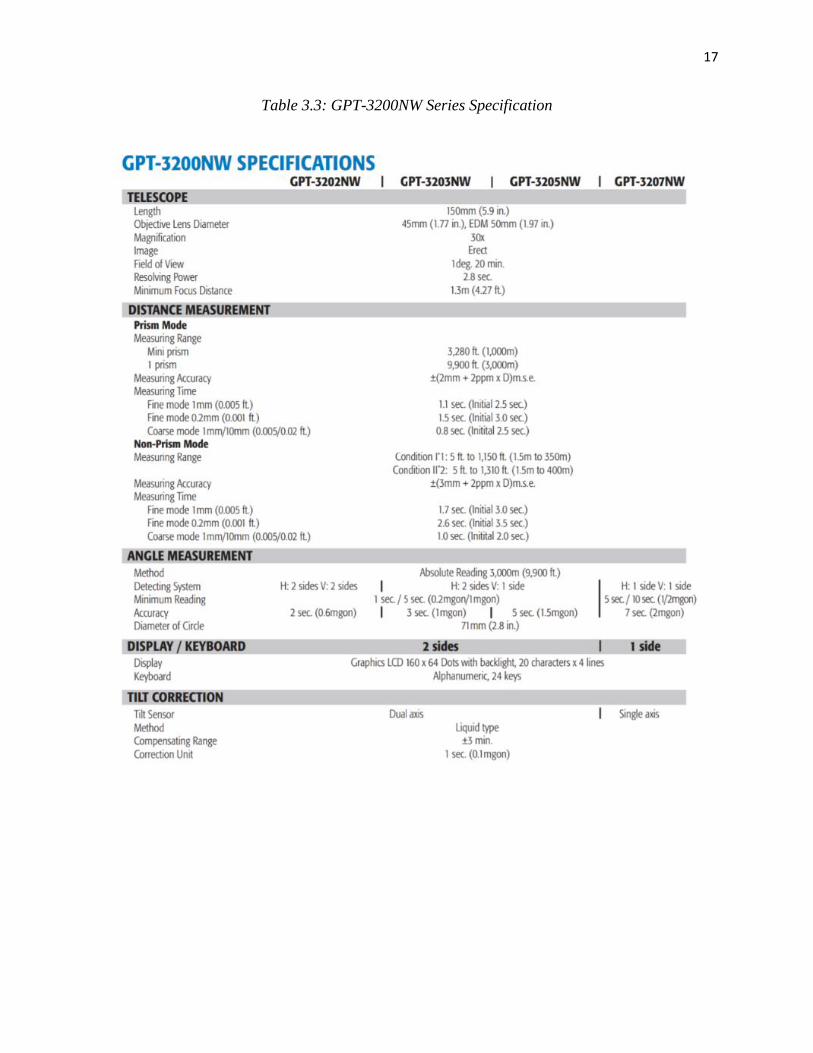
Table 4.3: Case Study 1 (7-Sec Instrument) – Azimuths of Each Side
Figure 4.1: Latitude and Departure Components of a Traverse Side.
Then, the latitudes of all sides are added to determine the latitude component, EL, of the
total longitudinal error of closure, EC. Similarly, the departures of all sides are added to obtain
the departure component, ED, of the total longitudinal error of closure, EC. Subsequently, these

22
two components are combined to calculate the full magnitude of the longitudinal error of closure
as follows:
𝐸𝐶 = √𝐸𝐿2 + 𝐸𝐷
2
EC, is present in most closed polygonal traverses. This study attempts to correct it via a different
approach than the classical Compass Rule. At this point in the calculations, the needed full
Closure Correction, is 𝐶𝐶 = −𝐸𝐶.
Compass Rule
As indicated above, the two horizontal components (latitude and departure) of the vector
representing the total longitudinal error of closure can be straightforwardly determined for each
closed traverse. Therefore, the vector corresponding to the total closure correction, CC, is known.
The widely used Compass Rule corrects the error of closure, EC, by applying assumed
corrections to each horizontal component of each side of the traverse. These corrections are
proportional to the length of each side. Thus, to determine the Compass Rule correction in
latitude, 𝐶𝐿𝑖, and in departure, 𝐶𝐷𝑖
, for each side i, the following two expressions were used:
𝐶𝐿𝑖= −𝐸𝐿
𝐿𝑖
𝑃 and 𝐶𝐷𝑖
= −𝐸𝐷
𝐿𝑖
𝑃
Where 𝐿𝑖 is the length of side i and P is the perimeter of the full closed traverse. Table 4.4 shows
these calculations for the example traverse we are considering in this section. It should be
mentioned that the above referred corrections are not actual corrections. They just represent a

23
rational approach to assume corrections for each side of the traverse and attain zero total error of
closure.
Table .4.4: Case Study 1 (7-Sec Instrument)- Longitudinal Balancing via Compass Rule
During this procedure it is possible to calculate the Longitudinal Precision Ratio (LPR)
using the following expression:
𝐿𝑃𝑅 =𝐸𝐶
𝑃=
1
(𝑃/𝐸𝐶)=
1
𝐷
The LPR is most commonly expressed as 1:D, where 𝐷 = 𝑃/𝐸𝐶. Sice P is a much larger number
than 𝐸𝐶, D results as a large number compared to the unit numerator in the LPR which is
commonly referred to as the longitudinal precision of the traverse. In civil engineering projects,
the usually minimum required longitudinal precision is 1:10,000, but depending on the type of

24
project, much higher precisions could be required. Here, the word higher indicates a larger
denominator D in the expression for LPR. In Table 4.4, it is observed that the longitudinal
precision of the considered example traverse was 1:18,819.
Proposed Procedure to Balance the Longitudinal Error of Closure
Even though the Compass Rule fully balances (reduces it to zero) the total error of
closure, 𝐸𝐶, it does not necessarily apply a true correction to each side of the traverse. This
motivated Professor Gustavo Maldonado to analyze the sensitivity of 𝐸𝐶 to small variations in
lengths of each side of the traverse. It was thought this sensitivity analysis could identify the
side(s) with the erroneous lengths and the magnitude of these errors. If this were the case,
applying actual corrections to those particular sides will increase the original longitudinal
precision. This motivated the current work.
Table 4.5: Case Study 1 (1-Sec Instrument) – Overall Angular Error Balancing

25
Since this work only focuses in the longitudinal error of closure, it was preferred to
minimize the angular error of closure and its influence in the longitudinal one. Therefore, the
example traverse that was previously considered was remeasured employing a more accurate
total station instrument, the one-second Leica TRCP 1201+. This resulted in a negligible angular
error of closure (i.e., zero second). Tables 4.5 and 4.6 show the corresponding calculations with
measurements performed with the 1-sec TRCP 1201+ instrument. Table 4.6 shows the balancing
results corresponding to the Compass Rule approach, where it can be noticed that the 1-sec
instrument attained EC = 0.026 ft (vs EC = 0.029 ft with the 7-sec instrument), and LPR =
1/21,465 (vs LPR = 1/18,819 with the 7-sec instrument).
Table 4.6: Case Study 1 (1-Sec Instrument) – Longitudinal Balancing via Compass Rule
Since the denominator, 𝐷 = 𝑃/𝐸𝐶, of the longitudinal precision ratio, 𝐿𝑃𝑅 = 1/𝐷 is a
relatively large number, inversely proportional to 𝐸𝐶 (whose magnitude is small and needs to be

26
further reduced), it was decided to analyze the sensitivity of D (instead of 𝐸𝐶) to small variations
in the lengths of each traverse side. This assists the graphical visualizing of those sensibilities.
The sensitivity analysis of D was completed as follows. The length of each side was
changed by successive increments of ±0.01 ft and a new LPR = 1/D value was calculated after
each small variation in side length. These new values are referred to here as Pseudo LPR. Table
4.7 shows the differences in D after small increments or decrements in the lengths of each
traverse side. In this table, the originally measured distances, between two consecutive vertices,
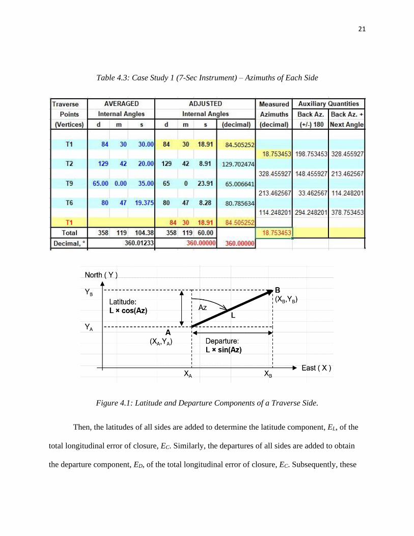
are highlighted in yellow. Figures 4.2-4.5 show the sensitivities of D in the Pseudo LPRs.
Table 4.7: Case Study 1 (1-Sec Instrument) – Sensitivity of Pseudo Longitudinal Precision Ratio
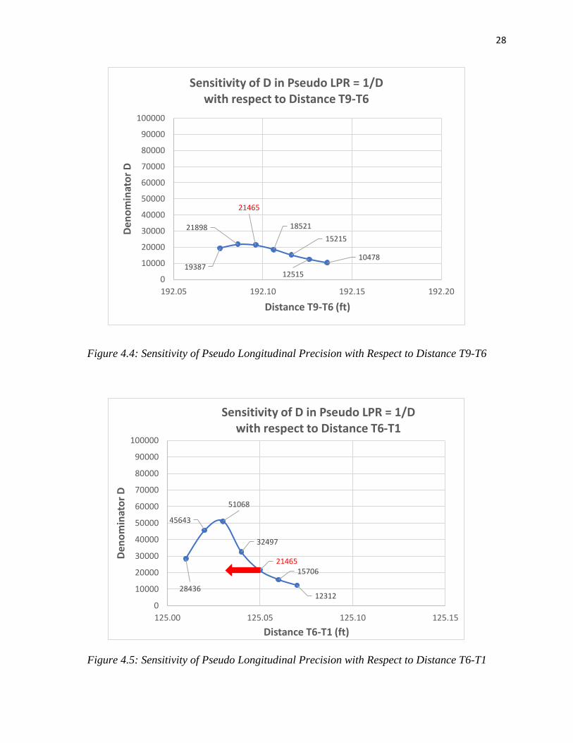
Figures 4.2-4.5 clearly show that, in this case, the Pseudo LPR is more sensitive to the
variations in lengths of sides T2-T9 and T6-T1. Therefore, those two sides are considered as the
most likely cause of the longitudinal error of closure for the traverse. Based on this observation,
the sides that were determined more sensitive were slightly altered in length to attain higher
Pseudo LPRs. Thus, the length of side T2-T9 was increased from 98.417 ft to 98.437 ft and the
length of side T6-T1 was decreased from 125.050 ft to 125.040 ft (see arrows in red). In both
cases, the lengths were chosen to be closer to the sensitivity peak shown in Figures 4.3 and 4.5.

27
Figure 4.2: Sensitivity of Pseudo Longitudinal Precision with Respect to Distance T1-T2
Figure 4.3: Sensitivity of Pseudo Longitudinal Precision with Respect to Distance T2-T9
13967
1736021465
2437823218
19290
0
10000
20000
30000
40000
50000
60000
70000
80000
90000
100000
134.85 134.90 134.95 135.00
Den
om
inat
or
D
Distance T1-T2 (ft)
Sensitivity of D in Pseudo LPR=1/Dwith respect to Distance T1-T2
12113
15499
21465
34550
7781380961
35358
0
10000
20000
30000
40000
50000
60000
70000
80000
90000
100000
98.35 98.40 98.45 98.50
Den
om
inat
or
D
Distance T2-T9 (ft)
Sensitivity of D in Pseudo LPR=1/Dwith respect to Distance T2-T9
28
Figure 4.4: Sensitivity of Pseudo Longitudinal Precision with Respect to Distance T9-T6
Figure 4.5: Sensitivity of Pseudo Longitudinal Precision with Respect to Distance T6-T1
19387
21898
21465
18521
15215
12515
10478
0
10000
20000
30000
40000
50000
60000
70000
80000
90000
100000
192.05 192.10 192.15 192.20
Den
om
inat
or
D
Distance T9-T6 (ft)
Sensitivity of D in Pseudo LPR = 1/Dwith respect to Distance T9-T6
28436
45643
51068
32497
2146515706
123120
10000
20000
30000
40000
50000
60000
70000
80000
90000
100000
125.00 125.05 125.10 125.15
Den
om
inat
or
D
Distance T6-T1 (ft)
Sensitivity of D in Pseudo LPR = 1/Dwith respect to Distance T6-T1

29
After the two new side lengths were adopted, the longitudinal error of closure was
recalculated as seen in Table 4.8. Its value was substantially reduced from 0.026 ft to 0.003 ft,
and the Pseudo LPR changed from 1:21,465 to 1:172,787. Additionally, after this balancing was
implemented, the Compass Rule was applied to further balance the traverse and bring EC to zero.
Table 4.8: Case Study 1 (1-Sec Instrument) – Longitudinal Balancing via the Proposed
Approach
Then, starting from a vertex with known or set coordinates (XT1=400.000 ft and
YT1=600.000 ft), the Northing (Y) and Easting (X) coordinates of the remaining vertices were
determined by adding the components of each subsequent side. This is completed around the

30
perimeter of the traverse until the Northing and Easting coordinates of all vertices are
determined. To calculate the new value of the perimeter, the distance formula is used between
two consecutive vertices √(𝑥2 − 𝑥1)2 + (𝑦2 − 𝑦1)2, and these new distances were added to find
the perimeter of the polygon. The final coordinates are presented in Table 4.9.
Table 4.9: Case Study 1 (1-Sec Instrument) – Vertex Coordinates after New Balancing Approach
In summary, the proposed balancing approach is based on a sensitivity analysis of the
denominator D (in the longitudinal precision ration, LPR=1/D), with respect to small variations
in the lengths of all sides of the traverse, considering each of them independently. This analysis
identifies the sides that produce the most noticeable increases in D. Those sides are altered in
length to maximize D. This substantially reduces the longitudinal error of closure of the traverse.
31
However, EC is not zero yet. At that point, the Compass Rule is used to fully close the remaining
gap, attaining EC=0.
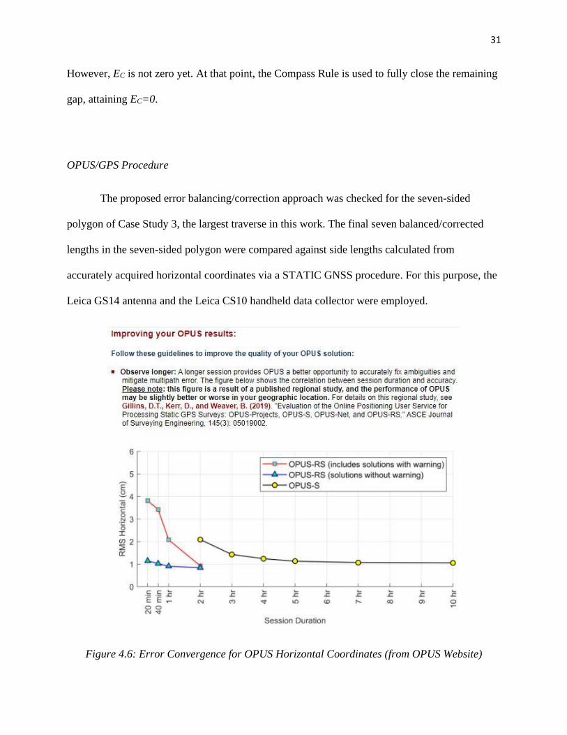
OPUS/GPS Procedure
The proposed error balancing/correction approach was checked for the seven-sided
polygon of Case Study 3, the largest traverse in this work. The final seven balanced/corrected
lengths in the seven-sided polygon were compared against side lengths calculated from
accurately acquired horizontal coordinates via a STATIC GNSS procedure. For this purpose, the
Leica GS14 antenna and the Leica CS10 handheld data collector were employed.
Figure 4.6: Error Convergence for OPUS Horizontal Coordinates (from OPUS Website)

32
The GNSS antenna was stationed during a minimum of four hours on each marked fixed
ground point (vertex) of the traverse. According to Figure 4.6, extracted from OPUS website, at
four continuous hours of STATIC data (S) collection, the root mean square (RMS) error is about
1.2 cm. It should be mentioned that about 8 hours of continuous collection time is required to
reduce the RMS value to 1 cm. Since the battery of our GNSS instruments was fully depleted at
approximately 6 hours of continuous use, it was decided to capture satellite data during a
minimum of four hours.
When analyzing the type of coordinate errors produced by STATIC GNSS approaches,
the mean value of those errors approaches zero and the corresponding RMS value approaches the
Standard Deviation, σ, of the error. So, in this case, RMS ≈ σ. Since it is assumed that this is a
Gaussian process, it is possible to apply the well-known 68-95-99.7 statistical rule. That is, 68%
of the observations have an error within the ± σ = ± 1.2 cm interval; 95% of the observations
falls in the ± 2 σ = ± 2.2 cm error interval; and 99.7% of the observations are within the ± 3 σ =
±3.6 cm interval. This provides a sense of the horizontal coordinate accuracy attained by the
selected benchmarking STATIC GNSS approach in this work. That is, after 4 hours of data
collection, we should expect that only 68% of the point data submitted, processed, and returned
to us by OPUS is with a ± 1.2-cm error. The remaining 32% has higher errors which may reach
up to 3.6 cm. In other words, statistically, about 2 out of 3 submissions to OPUS would return
data with an error in the ± 1.2 cm range. The third point is likely to have an error in the ± 2.4 cm
range, and very unlikely it may reach ± 3.6 cm. We submitted 7 points. So, it is expected that 4
or 5 of them have a ± 1.2-cm error and 3 or 2 of them have a ± 2.4-cm error.
The data collected by the Leica GS14 antenna is stored in a memory card (MicroSD card)
as a computer file with extension “.m00” (which corresponds to a ComputerEyes Animation

33
format). That file is then extracted and uploaded directly to https://geodesy.noaa.gov/OPUS/, the
website of OPUS. The submission requires to complete the below steps. Additionally, Figure 4.7
shows the online screen at OPUS website, where the file is to be submitted.
Figure 4.7: Sample OPUS Online Screen to Submit Captured GNSS Data
Steps to submit a file to OPUS:
a. First, use the above Internet address to visit the OPUS website to submit your .m00 file.
b. In the “Choose File” field enter the name of your Leica file with extension “.m00”.

34
c. Select GS14 antenna as the antenna in the dropdown menu that has “NONE” selected as
default.
d. Enter your antenna height. In our case it was “1.8” meters.
e. Enter the email address where you prefer to receive the processed data back.
f. The “Options” field refers to the amount of data you wish to receive back from OPUS. If
this option is left without selection, the default will be assumed. That is, the file you will
receive will be in the “standard” format. The other alternative option is “extended” which
will include more information.
g. Finally, select the “Upload to Static” option.
OPUS sends the corrected vertex coordinates in meters on various systems of references,
such as Universal Transverse Mercator (UTM), Zone 17, or the Georgia East State Plane
Coordinate System (SPCS). The processed data received from OPUS for all seven vertices is
included in Appendix D. These coordinates were employed to calculate the distances of all seven
sides of the traverse. Then, these measurements were employed as benchmarks. The distances
obtained with the proposed error-closing approach were compared against these seven
benchmarks.

35
CHAPTER 5
RESULTS
Case Study 1
Four-Sided Polygon 1: North Traverse at El Sombrero Restaurant Site
The first case considered was chosen to be a traverse located at the site of El Sombrero
Restaurant in Statesboro, GA. This traverse was measured twice. Once on March 25-27, 2019,
with a seven-second instrument, and again on Wednesday, April 10, 2019, with a one-second
instrument. This was completed by a group of undergraduate and graduate students under the
direction of Professor Maldonado.
Figure 5.1: Case Study 1: El Sombrero Restaurant – North Traverse

36
The area enclosed by this traverse was approximately 0.39 acres. Four control points
were chosen and marked with a nail to represent the total study area. These four points were
selected following clear lines of sight between two contiguous points, which allowed the
completion of accurate and undisturbed measurements with the two mentioned total-station
instruments. As shown in Figures 1.1 and 5.1, the vertices of this traverse were T1, T2, T9, and
T6. Points T1 and the one used as its backsight, T14, were geolocated via the RTK GNSS
procedure. The results of this case were described in the previous section of this document, when
introducing the proposed new balancing approach.
The implementation of the classical Compass Rule generated an original longitudinal
precision ratio LPR=1/21,465, whereas the proposed new error-balancing approach produced a
Pseudo LPR = 1/172,787.
Case Study 2
Four-Sided Polygon 2: South Traverse at El Sombrero Restaurant Site
This case also considers a quadrilateral closed traverse but with larger dimensions than
the traverse of Case Study 1. The enclosed area of the South traverse is approximately 1.13
acres. This traverse and its vertices are shown in Figures 1.1 and 5.2. In this instance, all
measurements were completed employing first a seven-second instrument and then were
repeated with a one-second instrument. The seven-second instrument generated an angular error
of closure of -5 seconds. Even though this was relatively low, this traverse was remeasured with
a one-second instrument which resulted in a 0-second angular error of closure, as observed in
Table 5.1. The second measurements are considered more accurate and were selected to proceed

37
with the proposed sensitivity analysis. Since the angular error of closure was zero second, it was
expected that it would not affect the longitudinal one. This South traverse contained one vertex,
T1 (or T01), common to the Case 1 traverse. The remaining points T12, T15 and T16, were
chosen for visibility reasons and marked with steel nails on the ground, as in the previous
traverse.
Figure 5.2: Case Study 2: El Sombrero Restaurant – South Traverse
The employed one-second instrument generated an error of closure EC = 0.033 ft and a
longitudinal precision ratio LPR = 1/29,477. The calculations leading to the classical Compass
Rule error-balancing approach are presented in Table 5.2. The sensitivity analysis involving
small variations of all four sides is presented in Table 5.3, where the originally measured side
lengths are highlighted in yellow and the adopted final lengths are marked in red.

38
Table 5.1: Case Study 2 (1-Sec Instrument) – Overall Angular Error Balancing
Table 5.2: Case Study 2 (1-sec instrument) – Longitudinal Balancing via Compass Rule

39
Table 5.3: Case Study 2 (1-sec instrument) – Sensitivity of Pseudo Longitudinal Precision Ratio
The sensitivity of D with respect to each side of this traverse is graphically shown in
Figures 5.3-5.6. In those figures, the points corresponding to the original measurements show the
value of D in red. After observing these graphs, it was decided that the proposed balancing
procedure be implemented by slightly changing the lengths of two sides.
The length of side T15-T16 was increased 0.02 ft, from 180.479 ft to 180.499 ft, and the
length of T16-T1 was decreased 0.03 ft, from 354.863 ft to 354.833. That is, in both cases these
lengths were modified to approach the peak of the two most pronounced sensitivity graphs. This
resulted in the balanced side components presented in Table 5.4. There, it is observed that the
longitudinal error of closure was substantially reduced to EC = 0.003 ft and the attained pseudo
longitudinal precision ratio was LPR = 1/355,314.

40
Figure 5.3: Sensitivity of Pseudo Longitudinal Precision with Respect to Distance T1-T12
Figure 5.4: Sensitivity of Pseudo Longitudinal Precision with Respect to Distance T12-T15
24461
27666
29477
28816
26112
22715
0
10000
20000
30000
40000
50000
60000
179.53 179.55 179.57 179.59
De
no
min
ato
r D
Distance T1-T12 (ft)
Sensitivity of D in Pseudo LPR = 1/Dwith respect to Distance T1-T12
19423
23595
2947737409
45299 46172
38930
0
10000
20000
30000
40000
50000
60000
263.25 263.27 263.29 263.31 263.33
De
no
min
ato
r D
Distance T12-T15 (ft)
Sensitivity of D in Pseudo LPR = 1/Dwith respect to Distance T12-T15

41
Figure 5.5: Sensitivity of Pseudo Longitudinal Precision with Respect to Distance T15-T16
Figure 5.6: Sensitivity of Longitudinal Precision with Respect to Distance T16-T01
21227
25153
2947732787
32993
29933
25629
0
10000
20000
30000
40000
50000
60000
180.45 180.47 180.49 180.51 180.53
De
no
min
ato
r D
Distance T15-T16 (ft)
Sensitivity of D in Pseudo LPR = 1/Dwith respect to Distance T15-T16
46979
56433
51035
38840
29477
23263
19056
0
10000
20000
30000
40000
50000
60000
354.82 354.84 354.86 354.88 354.90
De
no
min
ato
r D
Distance T16-T01 (ft)
Sensitivity of D in Pseudo LPR = 1/Dwith respect to Distance T16-T01

42
Table 5.4: Case Study 2 (1-Sec Instr.) – Longitudinal Balancing via the Proposed Approach
The final vertex coordinates attained after implementing the proposed balancing approach
are presented in Table 5.5.
Table 5.5: Case Study 2 (1-Sec Instrument) – Vertex Coordinates after New Balancing Approach

43
Case Study 3
Seven-Sided Polygon: Georgia Southern University - Statesboro Campus.
To further test the proposed method, a larger seven-sided polygon was chosen. It is
located on the Statesboro Campus of Georgia Southern University, enclosing an area of
approximately 6.82 acres. It is shown in Figures 1.2 and 5.7. Its seven vertices were selected so
unobstructed lines of sight were available between two consecutive vertices.
Figure 5.7: Case Study 3- Seven-Sided Traverse at Statesboro Campus
Initially, the following arbitrary coordinates were chosen for Vertex 1, Northing =
200.000 ft and Easting = 400.000 ft. Additionally, an approximate azimuth of 67° was assigned
Vertex 2900.408,412.414
Vertex 31191.350, 704.517
Vertex 41156.079, 1052.098
Vertex 5970.956, 864.349
Vertex 6619.39, 622.37
Vertex 799.91,
102.68
Vertex 1400.000, 200.000
0
200
400
600
800
1000
1200
0 200 400 600 800 1000 1200 1400
No
rth
ing
(ft
)
Easting (ft)
CAMPUS Traverse via 1-sec Total-Station Instrument
44
to side 1-2. Two of its vertices coincide with two Georgia Southern University official
benchmarks. Vertex 4, at the entrance of the Carruth building parking lot, is fixed point GSU 01.
Vertex 7, at the parking lot between the Engineering Building and the Performing Arts Center, is
fixed point GSU 27.
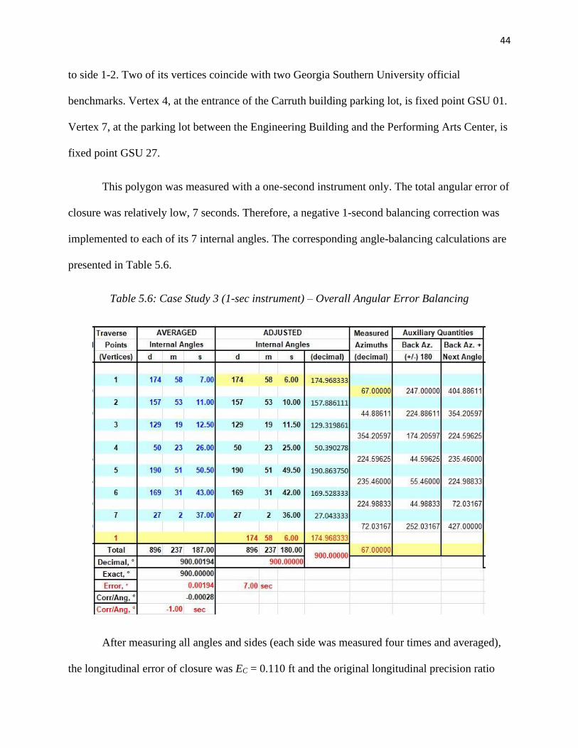
This polygon was measured with a one-second instrument only. The total angular error of
closure was relatively low, 7 seconds. Therefore, a negative 1-second balancing correction was
implemented to each of its 7 internal angles. The corresponding angle-balancing calculations are
presented in Table 5.6.
Table 5.6: Case Study 3 (1-sec instrument) – Overall Angular Error Balancing
After measuring all angles and sides (each side was measured four times and averaged),
the longitudinal error of closure was EC = 0.110 ft and the original longitudinal precision ratio

45
was LPR = 1/27,653, as seen in Table 5.7. Then, the classical Compass Rule was employed to
balance the latitude and departure components of each side, as indicated in Table 5.7.
Table 5.7: Case Study 3 (1-sec instrument) – Longitudinal Balancing via Compass Rule
Then, the balancing obtained with the Compass Rule was stored for comparison purposes
and the same sensitivity analysis, used in the previous two cases, was implemented for this
polygon. Table 5.8 shows all considered small variations for each side and their associated
denominator D of the corresponding pseudo longitudinal precision ratios. The line highlighted in
yellow contains the field measurements and the denominator, D = 27,653, of the original
longitudinal precision ratio, LPR = 1/27,653, corresponding to these field measurements.
Additionally, the numbers in red indicate the adopted new lengths for each side. In this case, the

46
sensitivity analysis prompted to change only three lengths, those of sides 1-2, 3-4 and 7-1.
Figures 5.8-5.14 show the sensitivity graphs corresponding to each of the seven sides.
Table 5.8: Case Study 3 (1-sec instrument) – Sensitivity of Pseudo Longitudinal Precision Ratio
Figure 5.8: Sensitivity of Pseudo Longitudinal Precision with Respect to Distance 1-2
22784
25988
28525
29218
27653
24708
21504
18631
16237
0
10000
20000
30000
40000
50000
543.52 543.56 543.60 543.64 543.68 543.72 543.76 543.80
De
no
min
ato
r D
Distance 1-2 (ft)
Sensitivity of D in Pseudo LPR = 1/Dwith respect to Distance 1-2

47
Figure 5.9: Sensitivity of Pseudo Longitudinal Precision with Respect to Distance 2-3
Figure 5.10: Sensitivity of Pseudo Longitudinal Precision with Respect to Distance 3-4
18232
20887
23769
26335
27653
27041
24834
21983
19206
0
10000
20000
30000
40000
50000
412.12 412.16 412.20 412.24 412.28 412.32 412.36 412.40 412.44
De
no
min
ato
r D
Distance 2-3 (ft)
Sensitivity of D in Pseudo LPR = 1/Dwith respect to Distance 2-3
13927
16008
18753
22481
2765334692
42717
46666
42095
0
10000
20000
30000
40000
50000
349.14 349.18 349.22 349.26 349.30 349.34 349.38 349.42
De
no
min
ato
r D
Distance 3-4 (ft)
Sensitivity of D in Pseudo LPR = 1/Dwith respect to Distance 3-4

48
Figure 5.11: Sensitivity of Pseudo Longitudinal Precision with Respect to Distance 4-5
Figure 5.12: Sensitivity of Pseudo Longitudinal Precision with Respect to Distance 5-6
19255
22039
24889
27076
27653
26303
23722
20839
18190
0
10000
20000
30000
40000
50000
263.52 263.56 263.60 263.64 263.68 263.72 263.76 263.80
De
no
min
ato
r D
Distance 4-5 (ft)
Sensitivity of D in Pseudo LPR = 1/Dwith respect to Distance 4-5
17578
20150
23039
25830
27653
27622
25755
22951
20067
0
10000
20000
30000
40000
50000
426.64 426.68 426.72 426.76 426.80 426.84 426.88 426.92 426.96
De
no
min
ato
r D
Distance 5-6 (ft)
Sensitivity of D in Pseudo LPR = 1/Dwith respect to Distance 5-6
49
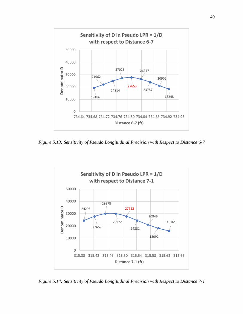
Figure 5.13: Sensitivity of Pseudo Longitudinal Precision with Respect to Distance 6-7
Figure 5.14: Sensitivity of Pseudo Longitudinal Precision with Respect to Distance 7-1
19186
21962
24814
27028
27653
26347
23787
20905
18248
0
10000
20000
30000
40000
50000
734.64 734.68 734.72 734.76 734.80 734.84 734.88 734.92 734.96
De
no
min
ato
r D
Distance 6-7 (ft)
Sensitivity of D in Pseudo LPR = 1/Dwith respect to Distance 6-7
24298
27669
29978
29972
27653
24281
20949
18092
15761
0
10000
20000
30000
40000
50000
315.38 315.42 315.46 315.50 315.54 315.58 315.62 315.66
De
no
min
ato
r D
Distance 7-1 (ft)
Sensitivity of D in Pseudo LPR = 1/Dwith respect to Distance 7-1

50
In figures 5.8, 5.10, and 5.14, it is clearly observed that originally measured lengths of
sides 1-2, 3-4, and 7-1 do not correspond to the peaks of denominator D. Therefore, they were
selected to be changed so they move closer to their respective sensitivity peaks. Thus, the length
of side 1-2 was decreased from 543.6555 ft to 543.6225 ft; side 3-4 was increased from 349.2748
ft to 349.3648 ft; and the length of side 7-1 was decreased from 315.5125 ft to 315.4825 ft. This
resulted in a substantial reduction of the longitudinal error of closure from EC = 0.110 ft to EC =
0.016 ft, and the original longitudinal precision ratio improved from LPR = 1/27,653 to a Pseudo
LPR = 1/193,727. At this point, the Compass Rule was applied to close the remaining small error
(0.016 ft). These calculations are shown in Table 5.9.
Table 5.9: Case Study 3 (1-Sec Instr.) – Longitudinal Balancing via the Proposed Approach
51
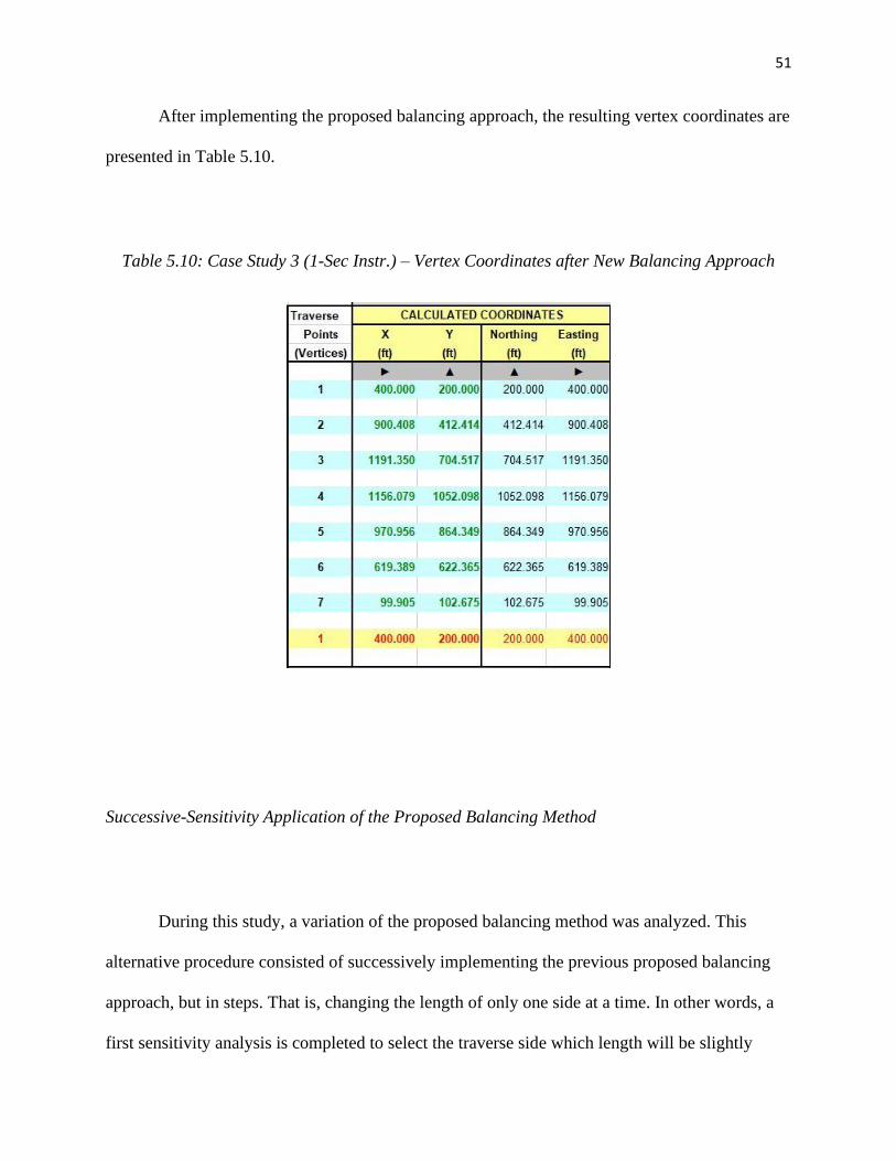
After implementing the proposed balancing approach, the resulting vertex coordinates are
presented in Table 5.10.
Table 5.10: Case Study 3 (1-Sec Instr.) – Vertex Coordinates after New Balancing Approach
Successive-Sensitivity Application of the Proposed Balancing Method
During this study, a variation of the proposed balancing method was analyzed. This
alternative procedure consisted of successively implementing the previous proposed balancing
approach, but in steps. That is, changing the length of only one side at a time. In other words, a
first sensitivity analysis is completed to select the traverse side which length will be slightly

52
modified. That side is the one associated with the largest sensitivity in D. After the length of this
single side is adjusted, a new improved pseudo longitudinal precision ratio is obtained. Then, a
second full sensitivity analysis of D with respect to all sides is performed again. This second
time, it may be necessary to reduce the magnitude of the small variations ± Δ applied to all side
lengths. This second run allows to select a second traverse side to adjust its length. After,
adopting a new length for this second side, an improved pseudo longitudinal precision ratio is
attained. This process could be repeated several times, as necessary.
Initially, it was considered that this alternative (and more time-consuming) approach,
may improve the final pseudo longitudinal precision ratio with respect to the final one obtained
in the original non-successive approach, the one that changes the lengths of several sides after a
single sensitivity analysis. This motivated the exploration of the successive sensitivity analyses.
Table 5.11: First Iteration of the Successive-Sensitivity Alternative Approach
The same polygon for Case Study 3 was used to test this alternative approach to balance
the longitudinal error of closure via successive sensitivity analysis. Table 5.11 shows the

53
numeric results for the first sensitivity iteration of this approach. This first run was completed
using ±Δ = 0.03 ft. It clearly indicates that D is most sensitive to variations in the length of side
3-4. Therefore, the length of this side is changed from its original field value 349.27475 ft
(average of four measurements) to 349.36475 ft. This results in a pseudo longitudinal precision
ratio LPR = 1/46,666, which represents an improvement with respect to the original LPR =
1/27,653. Table 5.11 presents all seven original field lengths in yellow (each is the average of 4
measurements in the field) and indicates the adopted length of side 3-4 in red.
Table 5.12: Second Iteration of the Successive-Sensitivity Alternative Approach
The results of the second sensitivity iteration (with ±Δ = 0.02 ft) are shown in Table 5.12.
From this second sensitivity analysis, it is inferred that now D is most sensitive to variations in
the length of side 7-1. Therefore, the length of this side was increased from 315.5125 ft to
315.4525 ft. This resulted in an error of closure EC = 0.013 ft and in a pseudo LPR = 1/231,303.
Similarly, Table 5.13 shows the results of the third sensitivity iteration (with ±Δ = 0.01
ft). This third sensitivity analysis shows that now D is most sensitive to variations in length of

54
side 3-4. Consequently, the length of this side was increased from 349.36475 ft to 349.37475 ft.
This resulted in an error of closure EC = 0.007 ft and in a pseudo LPR = 1/450.925.
Table 5.13: Third Iteration of the Successive-Sensitivity Alternative Approach
The final vertex coordinates resulting from each successive iteration (followed by closing
the remaining gap via the Compass Rule) are presented in Table 5.14:
Table 5.14: Vertex Coordinates after the 1st, 2nd and 3rd iteration.
First Iteration Second Iteration Third Iteration

55
Comparison of Proposed Approach against GNSS-Collected Data
To analyze the results of the proposed approaches (i.e., the simultaneous modifications of
side lengths and the successive modifications of them), their resulting final side lengths were
compared against accurate side lengths calculated from vertex coordinates obtained via GNSS.
In other words, this comparison was to discern if the proposed approach was correcting the side
lengths or if it was balancing them.
For this purpose, the Leica GS14 antenna was used in STATIC mode. It was setup on
each point of the seven-sided polygon to collect GNSS coordinate data during four or more
continuous hours per vertex. The GNSS/OPUS procedure, detailed in Methodology, was
followed for each point. The processed (corrected) coordinate data was received back from
OPUS, in meters at Grid Level. These coordinates, including orthogonal heights are shown in
Table 5.15.
Table 5.15: Received OPUS Coordinate Data for all Seven Vertices of Case Study 3
56
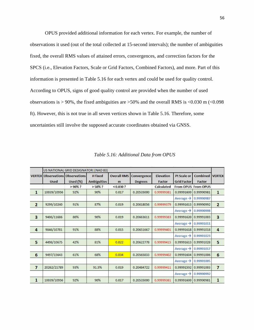
OPUS provided additional information for each vertex. For example, the number of
observations it used (out of the total collected at 15-second intervals); the number of ambiguities
fixed, the overall RMS values of attained errors, convergences, and correction factors for the
SPCS (i.e., Elevation Factors, Scale or Grid Factors, Combined Factors), and more. Part of this
information is presented in Table 5.16 for each vertex and could be used for quality control.
According to OPUS, signs of good quality control are provided when the number of used
observations is > 90%, the fixed ambiguities are >50% and the overall RMS is <0.030 m (<0.098
ft). However, this is not true in all seven vertices shown in Table 5.16. Therefore, some
uncertainties still involve the supposed accurate coordinates obtained via GNSS.
Table 5.16: Additional Data from OPUS

57
The coordinates were converted from meters to international feet. Then, all seven
distances, between two consecutive vertices, were calculated from those coordinates. This
resulted in distances at Grid Level. Therefore, the Combined Factors were employed to divide
the Grid-Level distances and thus converting them into Ground Level distances. For that
purpose, the Combined Factors of the two vertices defining a traverse side were averaged and
used for the distance between both. Those averaged Combined Factors are shown in Table 5.16.
Table 5.17: Vertex Coordinates, Side Lengths and Perimeters from 5 Different Approaches

58
Table 5.18: Discrepancies in Horizontal Lengths with Respect to GNSS-Measured Lengths
Figure 5.15: Discrepancies in Horizontal Lengths with Respect to GNSS-Attained Lengths
-0.20
-0.18
-0.16
-0.14
-0.12
-0.10
-0.08
-0.06
-0.04
-0.02
0.00
0.02
0.04
0.06
0.08
0.10
1-2 2-3 3-4 4-5 5-6 6-7 7-1 Per.
Dis
cre
pan
cies
in le
ngt
hs
(In
tern
atio
nal
Fo
ot)
Traverse Sides are designated as 1-2, 2-3, 3-4, 4-5, 5-6, 6-7 and 7-1.The Perimeter is designated as Per.
Discrepancies in Horizontal Lengthsof Traverse Sides and Perimeter
with Respect to GNSS Lengths (International Foot)
Compass Rule
Scheme 1
Scheme 2 - 1st Iter.
Scheme 2 - 2nd Iter.
Scheme 2 - 3rd Iter.

59
All seven side distances at Ground Level were calculated five times. One for each considered
case: (1) Plain Compass Rule (old classical approach); (2) Proposed Scheme 1 (simultaneous
sensitivity-based corrections of some sides plus Compass Rule to balance the remaining error of
closure); (3) Proposed Scheme 2 with 1 Iteration (sensitivity-based correction of one side plus
Compass Rule to balance remaining error of closure); (4) Proposed Scheme 2 with 2 Successive
Iterations (sensitivity-based successive correction of two sides plus Compass Rule to balance
remaining error of closure); and (5) Proposed Scheme 2 with 3 Successive Iterations
(sensitivity-based successive correction of three sides plus Compass Rule to balance remaining
error of closure). This is shown in Table 5.17. Additionally, Table 5.17 shows the calculated
perimeters at Ground Level for all 5 considered approaches.
For comparison purposes, the GNSS Ground-Level distances and perimeter were
subtracted from the distances and perimeters attained in the abovementioned five cases. These
discrepancies results are shown in Table 5.18. The two lines marked in red in Table 5.18 indicate
the sides presenting the largest discrepancies with respect to distances measured via GNSS. To
facilitate the visualization of these discrepancies they have been presented graphically in Figure
5.15.
Analysis of Results
The discrepancy information provided in Table 5.18, and visualized in Figure 5.15, is
analyzed here for each individual side of this seven-sided traverse.

60
Side 1-2: It is observed that the proposed scheme 2 with 3 iterations produced no distinguishable
discrepancy (0.000 ft) with the length calculated via GNSS. However, the Compass Rule
discrepancy is very small (0.002 ft) as well.
Side 2-3: The discrepancies presented by the Compass Rule (0.021 ft), by proposed scheme 1
(0.021 ft) and by proposed scheme 2 with 3 iterations (0.020 ft) are very similar to each other.
Almost no difference between them.
Side 3-4: In this side, the Compass Rule presents substantial less discrepancy (-0.017 ft) than
scheme 1 (0.074 ft) and scheme 2 with 3 iterations (0.083 ft).
Side 4-5: This side presents relatively large discrepancies, very similar in all three approaches
(from 0.085 ft to 0.086 ft).
Side 5-6: This side shows the largest discrepancies with respect to the measurement attained via
GNSS. For the three approaches the discrepancy amplitude is equal to 0.176 ft.
It should be noticed that Table 5.16 shows that the coordinates of vertex 5 were
calculated with only 42% of the collected observations and the RMS value of its error is 0.022 m
(larger than the 0.012 m expected). Similarly, the coordinates of vertex 6 were calculated with
61% of the observations and the RMS value of its error is 0.034 m which is the largest RMS
value of all seven vertices and almost 3 times much larger than the 0.012 m expected).
Therefore, it is possible that these two vertices were not acquired accurately by the GNSS
procedure. If that were the case, distance 5-6 cannot be used for comparison purposes.
Additionally, distances 4-5 and 6-7 could be affected by the wrong location of vertices 5 and 6.

61
Side 6-7: For this side, all three approaches present almost the same discrepancy magnitude,
ranging from 0.036 ft to 0.038 ft.
Side 7-1: In this side, the Compass Rule presents substantial less discrepancy (0.003 ft) than
scheme 1 (-0.028 ft) and much less than scheme 2 with 3 iterations (-0.058 ft).
Therefore, given the uncertainties involved in the accuracy of the GNSS-based
coordinates and respective lengths, the above discrepancies indicate that the proposed schemes to
balance/correct the error of closure, when applied to the seven-sided closed traverse, did not
present substantial evidence yet to indicate that they corrected the error of closure, rather than
balancing it. Given these uncertain results, we can only indicate that the proposed approaches
fully balance the error of closure. It will be necessary to repeat the collection of GNSS data for
this polygon, especially for vertices 5 and 6 to see if the proposed approaches effectively correct
the longitudinal error of closure. Alternatively, GNSS data could be obtained for the two
quadrilateral polygons or for new ones to full y test this.
An interesting observation is the fact that the proposed successive scheme performs better
than the Compass Rule when the full perimeter is compared. In that case the discrepancies in the
total length of the perimeter are -0.044 ft for the Compass Rule, 0.044 ft for scheme 1 and very
small, 0.007 ft, for scheme 2 with 3 iterations. This may still indicate that one of the two
proposed approaches, at least, may lead to truly correction of a substantial amount of the
longitudinal error of closure EC.

62
Virtual Case: Rectangular Traverse
This study investigated a particular case where the proposed approaches will not properly
identify the side with an erroneous length. Additionally, it was analyzed if the proposed
approaches correct, or just balance, the longitudinal error of closure, EC. For this purpose, a
virtual rectangular traverse (1000 ft × 500 ft), enclosing ~11.48 acres, was analyzed. It is shown
in Figure 5.16 with the exact coordinates of its four vertices. A selected small error of closure,
EC.=0.040 ft, was imposed in its first side, from vertex V1 to vertex V2. That is, the erroneous
length of side V1-V2 was considered 999.960 ft, instead of the correct 1000.000 ft. Furthermore,
it was assumed that all four internal angles were correctly measured to be exactly 90°00’00”
each. That is, no angular error of closure was imposed. Then, the Compass Rule and the
proposed simultaneous approach, scheme 1, were independently completed.
Figure 5.16: Virtual Rectangular Traverse with No Errors of Closure
V2: 1200.000,200.000
V3: 1200.000700.000
V4: 200.000,700.000
V1: 200.000,200.000
0
100
200
300
400
500
600
700
800
900
1000
0 100 200 300 400 500 600 700 800 900 1000 1100 1200 1300 1400
No
rth
ing
(ft
)
Easting (ft)
Virtual Rectangular Traverse

63
The error-balancing results from the application of the Compass Rule, and the resulting
balanced lengths and final vertex coordinates are shown in Tables 5.19 and 5.20. In those Tables,
it is clearly observed that the Compass Rule does not actually correct the longitudinal error of
closure but just balances it. The final vertex coordinates, resulting from the application of the
Compass Rule only, are not the exact ones, but close to the exact ones. Also, the final lengths of
the traverse sides are V1-V2: L1=999.973 ft (instead of the exact 1000.000 ft), V2-V3: L2=500.000
ft (exact!), V3-V4: L3=999.987 ft (instead of the exact 1000.000 ft), and V4-V1: L4=500.000 ft
(exact!). That is, two of them are not the exact ones.
Table 5.19: Virtual Rectangular Traverse – Error Balancing Via Compass Rule

64
Table 5.20: Virtual Rectangular Traverse – Final Vertex Coordinates Via Compass Rule
The sensitivity analysis of D with respect to lengths L1, L2, L3 and L4, is graphically
presented in Figure 5.17, where it can be observed that D is increased to very high values at
certain lengths of sides L1 (V1-V2) and L3 (V3-V4). Therefore, these four D-sensitivity graphs
(a), (b), (c) and (d), prompt us to vary the lengths of only sides, L1 and L3. However, only L1 is
the erroneous one. So, if we use the proposed simultaneous scheme 1, both sides L1 and L3 are to
be varied and this is not appropriate. After varying sides L1 from 999.960 ft to 1000.000 ft and L3
from 1000.000 ft to 999.960 ft, EC is back to the original magnitude of 0.04 ft. Then, the
subsequent application of the error-balancing Compass Rule results in the final vertex
coordinates shown in Table 5.21 which are similar but slightly different than those in Table 5.20,
where only the Compass Rule was employed.
Consequently, it is observed that the proposed simultaneous scheme 1 may not properly
identify the side length in error if it is parallel to another one. Therefore, it should be indicated
that, in these parallel-side cases, the proposed simultaneous scheme 1 is an error-balancing
approach, rather than an error-correcting one.

65
Figure 5.17: D-Sensitivity Analysis of Virtual Rectangular Traverse

66
Table 5.21: Virtual Rectangular Traverse – Error Balancing Via Proposed Simultaneous Scheme
Additionally, the use of the proposed successive scheme 2, in this rectangular traverse,
shows a similar behavior than scheme 1. That is, it is not able to properly identify the side with
the erroneous length if it is parallel to the other one. For example, if for the first iteration, we
modify side L1 (from 999.960 ft to 1000.000) the polygon would be truly corrected (not
balanced) and there will be no need for another iteration. On the other hand, if we start the first
iteration modifying side L3, (from 1000.000 ft to 999.960 ft) there would be no need to perform
another iteration to correct side L1, but this length modification will not correspond to a true
correction. It will be an error balancing approach and the final lengths of both sides will still
have an error.
Therefore, under the mentioned parallel conditions, it is evident that the proposed
schemes do not truly correct the errors but balance them. The successive scheme 2 may truly
correct the rectangular traverse, or similar one with parallel sides, only if the proper side (out of
the parallel one) is selected to be corrected.

67
CHAPTER 6
CONCLUDING REMARKS
In this study, three closed polygons were materialized and measured in the field to
implement and test two proposed new approaches to balance/correct the horizontal longitudinal
error of closure in land surveying traverses. Two of the traverses were quadrilateral polygons at
the North (~0.39 acres) and South (~1.13 acres) sections of a commercial site in Statesboro, GA.
One traverse was a seven-sided polygon (~6.82 acres) at the Statesboro Campus of Georgia
Southern University, and one traverse was a virtual rectangular one to analyze the behavior of
the proposed schemes when considering traverses with parallel sides.
The proposed two new approaches are sensitivity-based schemes 1 and 2, where the
amplitude of the horizontal longitudinal error of closure, EC, of a closed traverse is analyzed with
respect to small variations in the horizontal lengths of each traverse side, L1, L2, …, Ln (where n
is the total number of sides in the traverse). Since EC is a small number to be reduced to zero in
this study, for better visualization purposes it was decided to analyze the sensitivity of a quantity
D, inversely proportional to EC, to small variations of the side lengths. Since D is defined as
D=P/EC, where P is the full perimeter of the traverse, D is a relatively large number that
approaches infinity when EC approaches zero. As seen in the below expression, D is the
denominator of the original longitudinal precision ratio (LPR) of the traverse when its numerator
is forced to be equal to one. LPR defined as:
𝐿𝑃𝑅 =𝐸𝑐
𝑃=
1
(𝑃/𝐸𝑐)=
1
𝐷

68
In Land Surveying/Civil Engineering practice, LPR is usually expressed as LPR = 1:D. This
ratio is a good measure of the horizontal longitudinal precision attained by the original field
measurements. In this study, every time that the length of a side is modified, LPR is recalculated.
Since this recalculation involves modified lengths (not the original ones), it was preferred to call
the recalculated LPR as Pseudo LPR. If the applied length modifications were actual error-
correction ones, then LPR should remain named LPR (not Pseudo LPR). However, if the
modifications were just error-balancing ones, it is more appropriate to call the new calculation of
LPR as Pseudo LPR. The proposed new error-balancing/error-correction schemes, 1 and 2, are
briefly described as follows:
Scheme 1 performs a sensitivity analysis of D with respect to small variations, Δi, in all
lengths Li of the traverse, one at a time. This leads to D-sensitivity graphs where it clearly
identifies the length of each side that is associated with the peak of the corresponding D-
sensitivity curve. These sensitivity graphs are analyzed to assist in the adoption of simultaneous
changes in the lengths of a few sides of the traverse, not necessarily in all of them. In all cases,
the original measured lengths are modified (increased or decreased) so they approach the peak in
their respective D-sensitivity curves. During this process, it was observed that some sides were
already at their respective sensitivity peaks, or their D-sensitivity curves were relatively flat, so
modifying their lengths did not represent significant modifications in D. Since this scheme
simultaneously modifies the length of various traverse sides, it is also referred as the
Simultaneous Scheme.
Scheme 2 is a variation of scheme 1 requiring iterative sensitivity analyses. First, D-
sensitivity curves for all sides are determined in the same way as they were determined in scheme
1. However, in this alternative approach, only one side is selected to be modified per iteration.

69
This is the side showing the most pronounced D-sensitivity. The new modified length is adopted
and the EC and Pseudo LPR are recalculated to see the effect of this change. Then, a second
iteration is started which requires to produce all D-sensitivity curves again. These new curves
assist in modifying the length of a second side, the one showing the most pronounced D-
sensitivity curve. To perform the second iteration (and each subsequent one), it is necessary to
reduce the magnitude of the employed small variations, Δi, in the lengths of the traverse sides.
Then, a third or fourth iteration could be performed. After each iteration, EC and the Pseudo LPR
are recalculated to observe the effect of the applied length modification. In the study polygons,
After two or three iterations, EC would be substantially reduced, and D would be considerably
increased without the need to continue iterating. As it was the case in scheme 1, the remaining
small gap is closed via the classical Compass Rule. Due to the iterative characteristic of this
second proposed scheme, it is also referred as the Successive or Iterative Scheme. This second
scheme was only tested in the seven-sided polygon.
Both proposed schemes, the simultaneous and the successive one, substantially reduced
the magnitude of the horizontal longitudinal error of closure, EC, in the two, North and South,
four-sided traverses and in the seven-sided one. However, when considering the especial virtual
rectangular case, the successive scheme did not reduce the error of closure when modifying the
lengths of the two parallel sides that may contain the error. It was necessary to apply the
Compass Rule to balance and fully reduce EC to zero. Nevertheless, when the proposed
successive scheme was applied to the rectangular traverse, it did reduce EC to zero during the
first iteration. If, during this first iteration, the length of the right side was modified, then the
error of closure was fully and truly corrected. If the length of the wrong parallel side was
modified, EC was still reduced to zero, but the lengths of the parallel sides were not truly

70
corrected. They were just balanced. Therefore, it was realized that the proposed approach may
not truly correct EC in polygons with parallel sides.
To check if the proposed schemes were truly correcting EC, the vertex coordinates of the
seven-sided traverse were obtained via an accurate STATIC GNSS approach assisted by the
Online Positioning User Services, OPUS. These coordinates were then employed to obtain the
GNSS-based lengths of all seven sides to compare them against the final side lengths obtained
via the proposed schemes. This comparison was presented in Figure 5.15 and is here referred as
the discrepancy analysis. However, a couple of points (vertices 5 and 6) did not fully satisfy the
quality control requirements suggested by OPUS. Consequently, it is understood that the GNSS-
based coordinates of these two vertices (especially those of vertex 5) may have been acquired
with errors larger than expected. When comparing the final lengths obtained via the plain
Compass Rule or via the two proposed schemes against the GNSS-based lengths, side 5-6
presented the largest difference with a discrepancy=-0.176 ft, followed by side 4-5, with
discrepancies in the range of 0.085-0.086 ft. This further indicates that the GNSS-based
coordinates of vertex 5 may have not been accurately acquired, even after four continuous hours
of satellite data acquisition.
The plain Compass Rule showed almost the same very small discrepancy in the length of
side 1-2 as the iterative scheme 2. Similarly, the plain Compass Rule presented almost the same
discrepancy than those attained by schemes 1 and 2 in the lengths of sides 2-3, 4-5, 5-6 and 6-7.
Additionally, the plain Compass Rule presented less discrepancies in the lengths of sides 3-4 and
7-1 than schemes 1 and 2. On the other hand, when the length of the full perimeter was
compared, scheme 2 was much closer to the GNSS-based perimeter than scheme 1 which
showed less discrepancy than the plain Compass Rule. All these discrepancies were presented in

71
in Figure 5.15. Given the mentioned variations of the discrepancy results in the lengths of the
traverse sides, it was inconclusive if the suggested schemes were truly error-correction ones or
just error-balancing approaches, as the plain Compass Rule is. Further studies are needed to
arrive at a more conclusive statement on this regard. Nevertheless, both proposed new schemes
substantially reduce the longitudinal error of closure, EC.
The original longitudinal precision ratios, LPR, and the attained Pseudo LPR (before
applying the Compass Rule) are presented int Table 5.22, where it can clearly be inferred that the
proposed two schemes did considerably reduce the horizontal longitudinal error of closure.
Table 5.22: Original LPR and Attained Pseudo LPRs
Original
LPR
Pseudo LPR
after Scheme 1
Pseudo LPR after
Scheme 2 (3 iter.)
Case1: North, 4-sided
Polygon 1 / 21,465 1 / 172,787
Case 2: South, 4-sided
Polygon 1 / 29,477 1 / 355,314
Case 3: 7-sided
Polygon 1 / 27,653 1 / 193,727 1 / 450,925
Consequently, the proposed schemes do reduce the error of closure in an alternative fashion as
the plain Compass Rule does. It first applies corrections to certain selected sides (via a sensitivity
analysis of the denominator D of LPR=1/D), attaining a considerable reduction of the error of
closure before using the Compass Rule to fully close the remaining small gap.
Potential Improvements to be Considered

72
This work attempted to corroborate the use of the proposed schemes 1 and 2 in case study
three only, comparing the side lengths to lengths obtained via a STATIC GNSS approach.
However, that comparison provided inconclusive results. Therefore, it is suggested to extend that
comparison to case studies 1 and 2 to further investigate if the procedure was ultimately
correcting or just balancing the error of closure. Additionally, the proposed schemes only
consider the longitudinal error of closure and not the angular error of closure. It assumes the
angles do not play a role in the longitudinal error of closure and only focuses on whether to
stretch or shrink the lengths of those sides associated with the highest sensitivity of D.
Additionally, the proposed schemes do not identify the side that needs correction when the
erroneous length is parallel to another side. For instance, if sides one and three of a perfect
rectangular polygon are parallel and one of them is erroneously larger or shorter than the other,
either side could be shrunk or expanded to close the gap. The method examined in this study
cannot determine which of those two parallel sides contains the error without further human
intervention.
Further Studies
An additional undergraduate research study, sponsored by the Allen E. Paulson College
of Engineering and Computing of Georgia Southern University, was completed by undergraduate
student Lionel Ramirez Duran and the author of this thesis. This work investigated the
generation of closed form expressions for the denominator D, of the Longitudinal Precision Ratio
LPR, and its first partial derivatives with respect to the length of each traverse side, 𝜕𝐷
𝜕𝐿𝑖, where
i=1, 2,…, n, and n is the total number of sides of the traverse. These expressions are relevant

73
because they could substitute the time-consuming numerical sensitivity analyses employed in
this work. Preliminary results on this regard were presented in a short internal report to Georgia
Southern University. Since this report is not publicly available, it is attached to this thesis as
Appendix C. In that study, closed form expressions were obtained for the four-sided polygon of
Case 1. However, more work is still needed to find general expressions for a closed polygonal
traverse with any number of sides n.

74
REFERENCES
1. Peart, Mariah D., "Accuracy of 3D Point-Cloud and Photo-Based Models of City Street
Intersections" (2019). Electronic Theses and Dissertations. 1943
2. “What is OPUS.” National Geodetic Survey, https://geodesy.noaa.gov/OPUS/about.jsp.
Accessed 1 July 2021.
3. “Upload your data file.” National Geodetic Survey, https://geodesy.noaa.gov/OPUS/.
Accessed 1 July 2021.
4. “Convert Meters to Feet (u.s. Survey).” Kyles Converter,
http://www.kylesconverter.com/length/meters-to-feet-(u.s.-survey). Accessed 1 July 2021.
5. California Department of Transportation. Classification of Accuracy and Standards. April
2015, https://dot.ca.gov/-/media/dot-media/programs/right-of-way/documents/ls-
manual/05-surveys-a11y.pdf
6. Kavanaugh, Barry. Surveying Principles and Applications, Pearson Prentice Hall, July 4,
2008.
7. Mohammed Hashim Ameen, Abdulla Saeb Tais, Qayssar Mahmood Ajaj. “Evaluate
Accuracy between RTK GPS and Total Station in Adjustment Closed Traverse.”
International Journal of Interdisciplinary Environmental Studies, October 2019, pp. 1-15.
8. Alexander James Cook.” Can a Series of Resections Replace Conventional Traversing?”
February 2019.
9. H.Amini, S.Mehrdad.” Accuracy Assessment Of Different Error Adjustment Methods In
Closed Traverse Networks; Studying The Impact Of Different Observation Error Setups
In Different Geometrical Configurations.” The International Archives of the
Photogrammetry, Remote Sensing and Spatial Information Sciences, August 2020.
10. Charles D. Ghilani. “Where Theory Meets Practice: Grid versus Ground.”xyht,
https://www.xyht.com/professional-surveyor-archives/3088/. March 21, 2015
11. “Compass Rule.” ESRI, https://support.esri.com/en/other-resources/gis-
dictionary/term/29eb6d6a-177a-4b7b-ad05-1c06a0445438. Accessed 1 July 2021.
12. Topcon. GPT-3200NW Series. 2011, http://www.haagtrammell.com/docs/GPT-
3200NW_Broch_7010_2059-RevA-FINAL_lg.pdf

75
APPENDIX A
PROTOCOL TO PERFORM STATIC-GPS with GS14
SmartWorx Viva – How to Record Static Observation Data On-board GS Receivers in Rover Mode
STATIC OBSERVATION RECORDING OPTIONS
From the main menu select the Instrument icon.
© 2012 G360, LLC – All rights reserved
Next, choose the GPS settings.. icon.

76
Next, select the Raw Data Logging icon. That will open the Raw Data Logging Settings window, shown in the next figure.
In the Raw Data Logging Settings window, select the box next to Log data for post-processing and the options will be viewable. There are options to log data to the CS controller or the GS receiver (the receiver may also be referred to as GS sensor or GS Antenna). Logging the raw data to the SD card onboard the antenna will give you more flexibility. If you log it to the handheld controller, it will have to remain connected to the antenna for the entire session. To store the data in the SD card of the GS receiver, in the Log data to: field choose GS sensor. In the Logging starts: field choose Only within survey so that you can name your Point ID, input antenna height, and code if needed. In the Log data when: field select Static. In the Rate: field choose the epoch interval you wish to record observations. In the Data type: field you can choose either Leica format (MDB) or RINEX (for processing via OPUS). In this example we will be logging data in Leica format (MDB) to import the static data into Leica Geo Office (LGO) for processing. However, if you are going to process the data via OPUS, select RINEX.
The above settings, should be saved in a Working Style for convenience. If a Working Style is created for static surveys the user will be able to load the working style quickly instead of manually changing individual settings.
The SD card that will store the GNSS observation data should be placed in the GS receiver. The following figure shows an example of the LED configuration for the GS receivers when a formatted SD card is inserted. When the SD card is inserted into the receiver the LED next to the SD card icon will turn steady green (it looks as light green or even yellowish). This means the card is recognized and available for data recording. However, it is not recording data yet.

77
Leica GS14 with SD Card Inserted
PERFORMING SURVEY for STATIC OBSERVATIONS
To start the static survey and have it stored to the SD memory card (in the GS receiver) after you have made the proper settings, simply choose the Go to Work! icon from the main menu.

78
Next choose the Survey icon…
You can now enter the Point ID, Antenna height, and Code (see Code tab) as you prefer/need.
Then select F1 (Meas) function key. It is important that you enter all of the information for the survey point before you select to start measuring observations.

79
After you select to start measuring observations you will receive the message shown below.
Select the F6 (Yes) function key to exit the Survey application so that you can move to another part of your survey project. The GS receiver will continue to log raw data. IF BLINKING GREEN LIGHT ON GPS STOPS THE GPS IS NOT RECORDING DATA. LIGHT MUST BE BLINKING GREEN TO BE RECORDING DATA CORRECTLY.
SmartWorx will now report that the point has been stored. The job files will be stored on the CS controller (not in the antenna).
The GNSS raw data file (.m00 for the Leica Format) will be stored on the SD Card in the GS receiver (antenna).
If you plant to record data for a long period of time and need to leave the GS receiver, before you leave, observe that the SD card is recording the raw data. The LED for the SD card will blink green as shown in the following figure when the SD card is recording data.

80
Leica GS15 with SD Card Logging Data
THEN TURN OFF THE GPS WHEN YOU ARE DONE STORING DATA FORM THE SATELLITES BEFORE MOVING IT OFF THE FIXED POINT.

81
APPENDIX B
Two Point Acquisition for Closed Traverse Protocol
Leica TCRP 1201+ Robotic Total Station and Data Collector
Built Environment and Modeling LabGeorgia Southern University

82
Department of Civil Engineering and ConstructionOriginal Written by: Mariah Peart
Fall 2018 Adapted by: Jose Manzano
Summer 2021
Level & Laser Plummet
• Start by placing the instrument on any point of the closed traverse• Turn on the Robotic Total Station Instrument.• Level the instrument with the tripod stand, then complete the procedure with the leveling
screws.• Be sure to place laser plummet at the center location of the station (center of the nail).
Please note the following procedures are performed with a stylus. Procedures can vary without this tool.
Data Collector
• Turn on the Data Collector as a remote to the instrument.• The Instrument Mode Selection screen will appear, as shown in Figure 1.• Set Choose Sensor to “TPS”• Set Show at Startup to “Yes”• Then, press CONT
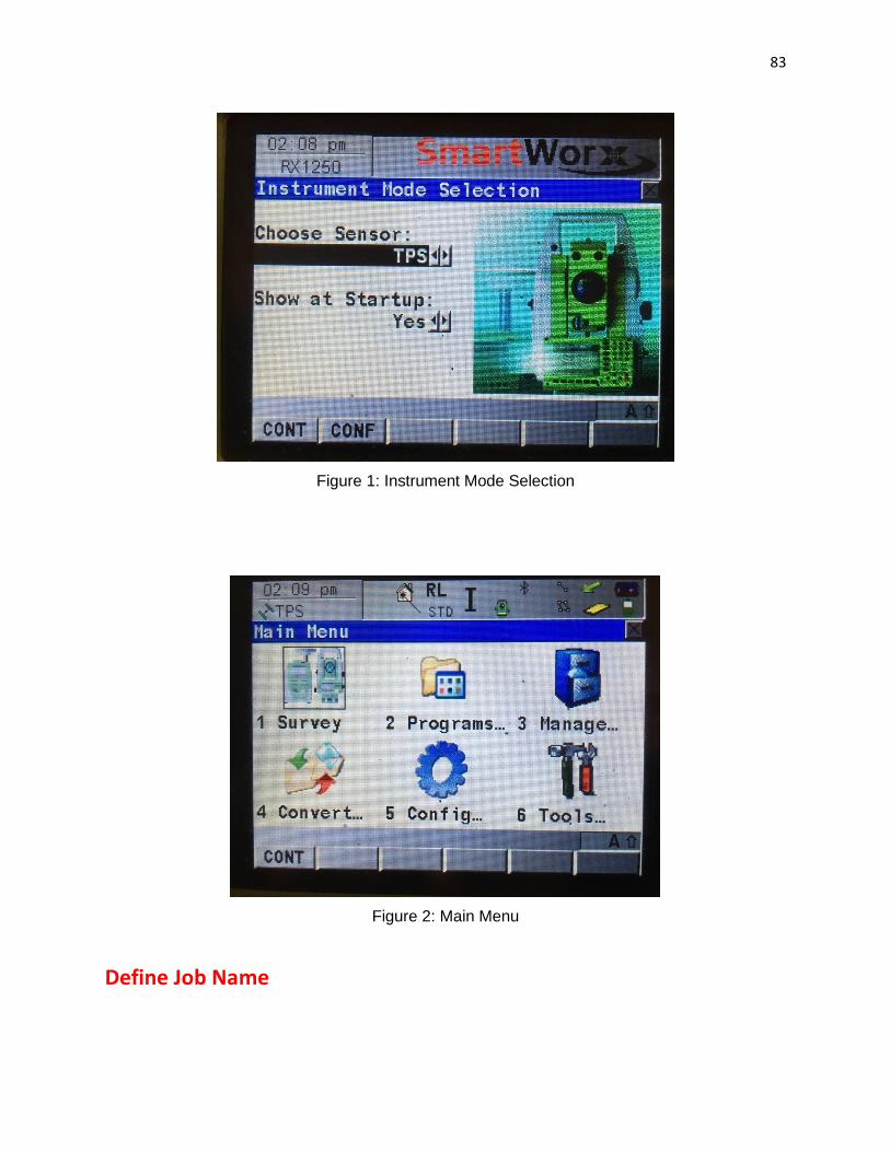
83
Figure 1: Instrument Mode Selection
Figure 2: Main Menu
Define Job Name

84
• From the main menu, select Manage, as shown in Figure 2.• From the Management window, select Jobs, as shown in Figure 3 (a).• From the Jobs window, select NEW, as shown in Figure 3 (b).• Name your New Job, then press STORE, as shown in Figure 3 (c).
Figure 3 (a): Management Window
Figure 3 (b): Job List

85
Figure 3 (c): Creating a New Job
Setting Instrument to Reflectorless
• From the main menu, select Manage. • From the Management menu, select Reflectors, choose Leica 360° prism, then press
CONT, as shown in Figure 4 (a - b).

86
Figure 4 (a): Management Menu (Reflectors)
Figure 4 (b): Reflector List

87
Station Setup
• From the main menu, select Survey.• The Survey Begin window will appear, as shown in Figure 5.• Check all parameters (Mainly, consider the “Job” and “Reflector” settings).• Then, select SETUP.
Figure 5: Survey Begin Window
The Station Setup Window will appear, as shown in Figure 6 (a).
• Set Method to “Set Azimuth”• Set Station Coord to “From Job”• Set new Station ID (this will be the I.D. for the current station)
• Select the current (highlighted) Station ID name.• The Data window will appear, as shown in Figure 6 (b).• Then, select NEW• The New Point screen will appear.• Input a new name for the Point ID• Input the Northing, Easting and Height (Elevation) as 0 ft for each the coordinates of the
current station.• Press STORE.• Be sure the new Point ID (Station ID) is highlighted, then select CONT.

88
• Measure and Input the Instrument Height.• Check Fixpoint Job name (same as the Job name that is created).• Then, select CONT.
Figure 6 (a): Station Setup
Figure 6 (b): Data Window

89
Set Station & Orientation – Set Azimuth
The “Set Stn & Ori – Set Azimuth” window will appear, similar to Figure 7.
• Name Backsight ID (This will be the name of the station where the reflector is located).
• Measure and Input the Reflector Height • Aim the instrument towards the reflector’s center point or press F12 for the instrument to
automatically find the reflector. • Set Azimuth to 0°0’0” • When the instrument is set, select DIST. • The distance is recorded as the distance between the current point and the backsight. • Then, choose SET. • The following message will appear, “Station and Orientation has been set.” • Then, press OK
Figure 7: “Set Stn & Ori – Known BS Point” Window
Note: If the Station Setup screen appears, as shown in Figure 6 (a), after the last step in the “Set Station & Orientation –Known BS Point” procedures, then press CONT.
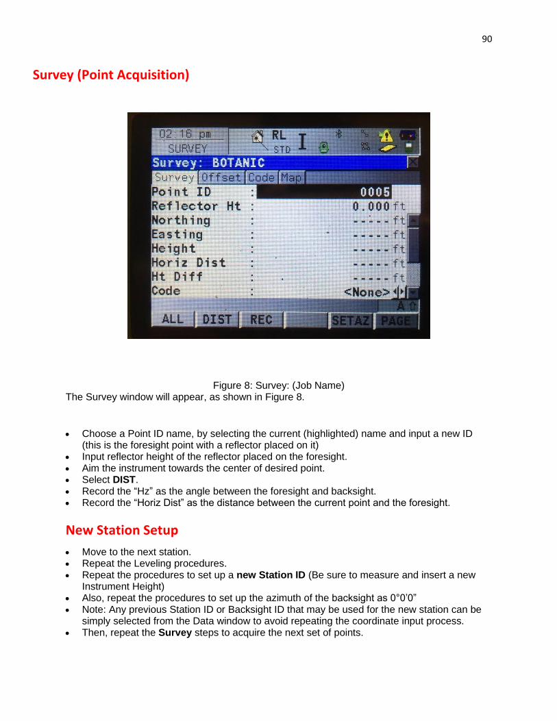
90
Survey (Point Acquisition)
Figure 8: Survey: (Job Name) The Survey window will appear, as shown in Figure 8.
• Choose a Point ID name, by selecting the current (highlighted) name and input a new ID(this is the foresight point with a reflector placed on it)
• Input reflector height of the reflector placed on the foresight.• Aim the instrument towards the center of desired point.• Select DIST.• Record the “Hz” as the angle between the foresight and backsight.• Record the “Horiz Dist” as the distance between the current point and the foresight.
New Station Setup
• Move to the next station.• Repeat the Leveling procedures.• Repeat the procedures to set up a new Station ID (Be sure to measure and insert a new
Instrument Height)• Also, repeat the procedures to set up the azimuth of the backsight as 0°0’0”• Note: Any previous Station ID or Backsight ID that may be used for the new station can be
simply selected from the Data window to avoid repeating the coordinate input process.• Then, repeat the Survey steps to acquire the next set of points.

91
APPENDIX C
Report on Undergraduate Research
Submitted to the Allen E. Paulson College of Engineering & Computing
Georgia Southern University
May 2021
A New Longitudinal Error Balancing Approach for Closed
Traverses – Mathematical Model
Student Authors
Lionel Ramirez Duran and J. Liweng Manzano
Faculty Mentors
Dr. Gustavo O. Maldonado and Dr. Marcel Maghiar
Department of Civil Engineering and Construction
Introduction and Objectives
A closed traverse is a mathematical approach commonly employed by land surveyors and civil
engineers to accurately determine the coordinates of ground control points (vertices of a closed polygon)
serving as reference benchmarks in boundary and construction surveys. This procedure involves the
measurement of a closed polygon. The elements that are measured are the horizontal internal angles and
the horizontal lengths of the sides of the polygon. While survey professionals perform these
measurements, there are two types of inevitable errors, angular and longitudinal ones. When the
instruments are properly calibrated and have adequate resolution, most of these errors can be reduced by
measuring numerous times each internal angle and each side of the polygon. However, with the current
modern surveying instruments it is still rare that these errors are fully eliminated obtaining exact
measurements.
Indefectibly, while performing the above-indicated traverse measurements and calculations there
will be remaining errors. They are called angular error of closure (AEC) and longitudinal error of closure
(LEC). Unfortunately, today does not exist a procedure that eliminates those errors. They can easily be
quantified but cannot be fully corrected. Currently, there are simple mathematical approaches that assist

92
in balancing these errors. The word “balancing” is purposely employed here to signify those errors of
closure are reduced to zero by distributing corrections to all involved elements, all internal angles, or all
side lengths. However, those “corrections” not necessarily are applied to the elements that were in error.
They are distributed to all of them. That is, it is assumed that all angles contribute to the AEC and that all
sides contribute to the LEC. Therefore, under that assumption, all elements are corrected a given amount
to make their global errors of closure to approach zero. The existing, classical, error-balancing approaches
are commonly employed by professional land surveyors and civil engineers while establishing accurate
ground-control points, i.e. vertices of the mentioned polygons, near construction projects and/or property
boundaries.
In this work, we will only concentrate in the LEC. An existing, classical, error-balancing
approach for LEC was developed by an American mathematician, Nathaniel Bowditch, and it was
published in 1807. The name of this approach is Compass Rule. Even today, after more than 200 years, it
is widely employed in polygonal closed traverses to balance LEC by stretching or shortening all polygon
sides by amounts proportional to their measured lengths. Certainly, the existing Compass Rule does not
properly correct the actual errors of closure. Errors may be concentrated in just one or in a few sides, not
necessarily in all of them. This study presents an alternative approach to balance errors of closure via
sensitivity analyses based on small variations of the lengths of all involved polygonal sides.
This work involves a two-fold goal: (1) Design a new mathematical approach to correct and
balance inevitable LEC, occurring in typical closed-traverse (i.e., closed-polygon) operations, performed
in Land Surveying/Geomatics applications. (2) Corroborate the effectiveness of the proposed new error-
correction/balancing scheme to attain higher longitudinal precisions than those typically obtained by
existing methods.
Methodology
This work uses a sensitivity-based analysis to reduce and balance the LEC resulting when
surveyors/engineers establish, and measure closed traverses in the field. Instead of determining the
sensitivity of LEC to small variations in lengths of the polygonal sides, we focus on the sensitivity to
those small variations of the denominator Y=(Perimeter/LEC) of the resulting original longitudinal
precision (OLP), which is defined as OLP=[1 / (Perimeter/LEC)]. This has been selected because Y is a
large number, closely related to LEC, and showing more ample variations than LEC itself. Actually, when
LEC approaches zero, Y approaches infinity. Each time that a small variation is provided to one side of
the polygon a new value of OLP is calculated. This new value is called herein as Pseudo Longitudinal
Precision (PLP). Here, we prefer to use the word pseudo because the OLP is modified each time that a
side variation is introduced. The actual longitudinal precision is OLP and depends on the original
measurements. It cannot change unless the LEC is properly corrected. Since we do not know if this
approach corrects or just balances the LEC (in a different manner than the Compass Rule), we prefer to
call the varying longitudinal precision as pseudo longitudinal precision, PLP.
For this work, we first established a four-sided traverse in the field and measured all its four
internal angles and the four horizontal lengths of its sides. This quadrilateral traverse was materialized
with steel nails around the main building, on the northern section of the El Sombrero restaurant site, at
879 Buckhead Dr, Statesboro, GA. The measurements and calculations corresponding to that traverse
were performed using a highly accurate one-second robotic total-station instrument as shown in Table 1.
Fortunately, the measurement of the four internal angles closed without error (AEC=0 sec). However, the
LEC (referred in Table 1 as Ec) was relatively high, 0.026 ft, with an OLP=1:21,465 (1 unit in 21,465
units).

93
Table 1: Four-sided traverse data and calculations,
with LEC = Ec.= 0.026, OLP=1/21,465, and Y=21,465.
Figure 1: Sensitivity analysis of Y (denominator of the PLP) with respect to small variations in the
lengths of each side of the closed traverse, defined by vertices T1, T2, T9 and T6.

94
Then, the sensitivity of the ratio Y=(Perimeter/LEC) was analyzed with respect to small, manually
selected, variations of the lengths of each polygonal side, one at a time. This variation of Y, with respect
to small variations in the length of each side (one side at each time), is presented in Figure 1(a-d).It
should be noticed that smaller variations steps improve the capture of sensitivity peaks in the previous
graphs. Corrections were applied to only the sides associated to the most pronounced variations of Y. The
remaining, and substantially reduced error of closure was balanced via the typical Compass Rule. This
final balancing step will attain zero closure in the horizontal lengths of the traverse sides.
Additionally, the Y value was
expressed in terms of the horizontal lengths
of sides Li (with i=1,2,3,4) and each side was
mathematically stretched or shortened
(varied) to observe the effect of such finite
variations in the overall Y value of the
involved closed traverse. The resulting finite
variational effects were graphically
interpolated using best-fit curves to observe
the continuous sensitivity of Y with respect to
each side of the polygon.
The methodology to obtain
mathematical expressions for the resulting
sensitivity graphs is based on the use of a
symbolic calculation computer algebra
system, named wxMaxima (version 20.06.6).
This methodology is presented in Figure 2,
where E is LEC, Li is the horizontal length of
side i, PLP is ε and Y is the ratio
(Perimeter/LEC). Figure 2: Sensitivity Methodology via wxMaxima
The resulting closed form expressions for 𝑌(𝐿𝑖) and its first derivative with respect to Li, 𝜕𝑌(𝐿𝑖)
𝜕𝐿𝑖, for
i=1,2,…,n, where n is the total number of sides, can be employed to accurately identify the amount of
variation needed in a particular side to effectively reduce the error of closure.
Results: Sample mathematical expression and corresponding graphs for an actual 4-sided traverse
This study analyzed the proposed approach in three different closed traverses. Two of them were
quadrilateral ones. One in the northern section of El Sombrero Restaurant site (enclosing 0.39 acres) and
one in its southern section (enclosing 1.13 acres). The remaining traverse was a much larger seven-sided
one (enclosing 6.82 acres), within the Statesboro Campus of Georgia Southern University.
Unlike the widely employed Compass Rule, the proposed balancing approach only applies main
corrections to a few sides. Table 2 shows the traverse calculations corresponding to the application of the
proposed scheme to the already introduced traverse example, the quadrilateral northern traverse. It is
observed that the proposed balancing approach only varied the lengths of two sides (those in red in Table
2, 94.437 ft and 125.040 ft) to reduce the LEC. The resulting calculations are presented in Table 2.

95
Table 2: Four-sided traverse data and calculations,
with LEC = Ec.= 0.003, PLP=1/172,787, and Y=1712,787
Figure 1 (b) and (d) shows the pronounced sensitivity of 𝑌(𝐿1,𝐿2,𝐿3,𝐿4) with respect to small
variations in the lengths of two sides, T2-T9 (b) and T6-T1 (d). In those graphs the number in red, 21.465,
indicates the value of Y when all sides were considered with their original measurements. By observing
Figure 1, the length of side T2-T9, shown in graph (b), must be increased to increase Y and reduce the
LEC. Similarly, the length of side T6-T1, shown in graph (d), must be decreased to increase Y and reduce
LEC. This was done by changing T2-T9 from 98.417 ft to 98.437 ft and by changing T6-T1 from 125.050
ft to 125.040 ft. These small changes resulted in a benefitting difference between PLP=1/172,787.vs
OLP=1/21,465.
For the same example, northern traverse, function 𝑌(𝐿1,𝐿2,𝐿3,𝐿4) = (Perimeter/LEC) is a function of
L1, L2, L3 and L4. After keeping L1, L3 and L4 constant, Y becomes a function of only L2, 𝑌(𝐿2), as seen in
the below expression, which is plotted in Figure 2. Recall that, in this example, L2 is the length of distance
T2-T9.
𝑌(𝐿2) =𝐿2 + 452.065
√(0.852110 ∗ 𝐿2 − 83.8811)2 + (51.5250 − 0.523362 ∗ 𝐿2)2
Similar expressions were attained for 𝑌(𝐿1), 𝑌(𝐿3),and 𝑌(𝐿4). Additionally closed-form expressions
were obtained for their first derivatives: 𝜕𝑌(𝐿1)/𝜕𝐿1, 𝜕𝑌(𝐿2)/𝜕𝐿2, 𝜕𝑌(𝐿3)/𝜕𝐿3, and 𝜕𝑌(𝐿4)/𝜕𝐿4. The
advantage of these expressions is that they assist in easily identifying the precise magnitudes of the side
lengths producing the highest value of Y (i.e., minimizing LEC). Figure 3 shows 𝜕𝑌(𝐿2)/𝜕𝐿2 vs L2, and it
clearly identifies the value of L2 (at the zero crossing of 𝜕𝑌(𝐿2)/𝜕𝐿2) where Y attains its highest value (i.e.,
lowest LEC).
Figure 3 clearly shows that variations in the original length of side 2, L2, generate a maximum
peak in ratio 𝑌(𝐿2) = (Perimeter/LEC). Additionally, Figure 4 can be used to identify the value of L2
producing that peak.
Conclusions and Closing Remarks
The proposed error balancing approach reduces the longitudinal error of closure and effectively closes the
traverses by correcting the lengths of a few of their sides. This contrast with the current and widely
employed error balancing technique, the Compass Rule, which balances the error of closure by applying
corrections to all traverse sides. Closed form expressions were obtained to assist in determining the proper
correction to be applied to each side and effectively close the traverse. Currently, this research has shown
that the proposed approach works. However, it is still necessary to corroborate if it corrects or simply
balance the error of closure. This corroboration will be implemented by accurately measuring a field

96
traverse using an accurate Global Navigation Satellite System (GNSS) device. Coordinate data will be
statically collected during four continuous hours at each traverse vertex. This should provide near-
centimeter accuracy in the coordinates of all vertices and their related side lengths.
Figure 3: Plot of 𝑌(𝐿2) = (𝑃𝑒𝑟𝑖𝑚𝑒𝑡𝑒𝑟/𝐿𝐸𝐶)(𝐿2) vs L2. Figure 4: Plot of 𝜕𝑌(𝐿2)/𝜕𝐿2 vs L2:

97
APPENDIX D
OPUS email regarding Vertex 1

98
OPUS email regarding Vertex 2

99
OPUS email regarding Vertex 3

100
OPUS email regarding Vertex 4

101
OPUS email regarding Vertex 5

102
OPUS email regarding Vertex 6

103
OPUS email regarding Vertex 7, captured on March 25, 2021

104
OPUS email regarding Vertex 7, captured on March 28, 2021