Optimized bounding boxes for three-dimensional treatment planning in brachytherapy

M. Lahanas, T. Kemmerer, N. Milickovic Department of Medical Physics & Engineering, Strahlenklinik, Klinikum Offenbach, 63069 Offenbach, Germany.

K. Karouzakis, D. Baltas, N. Zamboglou Department of Medical Physics & Engineering, Strahlenklinik, Klinikum Offenbach, 63069 Offenbach, Germany. and Institute of Communication & Computer Systems, National Technical University of Athens, 15773 Zografou, Athens, Greece.

Corresponding author: Michael Lahanas Dept. Of Medical Physics & Engineering Strahlenklinik Klinikum Offenbach Starkenburgring 66 63069 Offenbach am Main, Germany Tel.: +49 – 69 – 8405 –4480 E-mail: mlahanas@gmx.de

Lahanas Optimized bounding boxes for three-dimensional Page 2 of 2

ABSTRACT

It is sometimes necessary to determine the optimal value for a direction dependent quantity. Using a search technique based on Powell’s quadratic convergent method such an optimal direction can be approximated. The necessary geometric transformations in n-dimensional space are introduced. As an example we consider the approximation of the minimum bounding box of a set of three-dimensional points. Minimum bounding boxes can significantly improve accuracy and efficiency of the calculations in modern brachytherapy treatment planning of the volumes of objects or the dose distribution inside an object. A covariance matrix based approximation method for the minimum bounding box is compared with the results of the search method. The benefits of the use of optimal oriented bounding boxes in brachytherapy treatment planning systems are demonstrated and discussed. Key words: minimum bounding box, geometrical optimization, brachytherapy

Lahanas Optimized bounding boxes for three-dimensional Page 3 of 3

I. INTRODUCTION

The aim of this work was the development of an algorithm for the approximation of

the minimum bounding box of a three-dimensional object defined by a set of points. These points can be points of contours which describe objects such as organs. Normally the bounding box used is defined by the extreme coordinate values of the points with respect to some given global coordinate system. As objects in general are not aligned the bounding box can be very large compared to the dimensions of the object, see Figure 1. It is therefore useful to align the bounding box so that it encloses all the points but the volume is minimized. We call this bounding box a minimum-volume bounding box or minimum bounding box. An optimal oriented bounding box is an approximation of the minimum bounding box obtained from an optimization process. We present an optimization method for oriented bounding boxes and discuss the application of optimal oriented boxes in the field of brachytherapy.

Our anatomy based optimization method in the field of brachytherapy 1 uses bounding

boxes for a variety of reasons.

1) For the efficient calculation of dose-volume histograms (DVHs) of anatomical structures obtained from sampling points inside the three-dimensional triangulated objects using the test routines described by Lahanas et al. 2 The sampling points are required to be outside catheters and critical structures but inside the object. The generation time of sampling points can be reduced significantly using optimal oriented bounding boxes of the object, the critical structures and catheters.

2) For an optimal orientation of dose calculation grids for fast Fourier transform (FFT) based dose calculation methods, 3 the number of grid points inside an object has to be maximized. If the axes of the grid are given by the axes of the minimum bounding box of the object then the number of grid points inside the objects is maximal and this significantly increases the efficiency and accuracy of this method. 4

3) For the efficient determination of the volumes of objects which take into account catheters, a simple hit or miss Monte Carlo method with a large number of random points (> 105) inside the bounding box of each structure (e.g. organs) is produced. The ratio of the number of points inside the structure to the number of points inside the associated bounding box, which is maximal for minimum bounding boxes, is equal to the ratio of the structure volume to the bounding box volume. From the known bounding box volume, the volume of the structure is then calculated.

4) For the efficient calculation of DVHs of critical structures and the PTV a stratified sampling technique can be used 5 in which the regions also known as strata are defined by either optimal oriented bounding boxes or minimum enclosing spheres.

The minimum bounding box of a set of points can currently only be found with a

deterministic algorithm which requires an order of N3 operations for N points. An optimum oriented bounding box with a given accuracy can be found by a rather complicated systematic search. 6 For the minimum bounding sphere of a set of points very efficient algorithms are known. 7,8

Our method uses a gradient based optimization procedure to search an optimal

direction and orientation of the bounding box of a set of points using as a objective a minimum bounding box volume. This method can be used for other problems which require the determination of a direction which optimizes some quantity of interest. As an example, a problem in inverse planning in brachytherapy is the determination of an optimal position and orientation of a template for catheter insertion where the quantity to be optimized could be

Lahanas Optimized bounding boxes for three-dimensional Page 4 of 4

the cross-sectional area and volume covered by the template and accessible by the needles, taking into account critical structures.

II. METHODS

We present the currently known algorithms for the calculation of two and three-

dimensional minimum or optimum oriented bounding boxes. Thereafter our search based method is presented with the relevant coordinate transformations. Finally we describe how oriented bounding boxes are defined and how they can be used in a brachytherapy planning system.

A. Algorithms for the minimum bounding rectangle

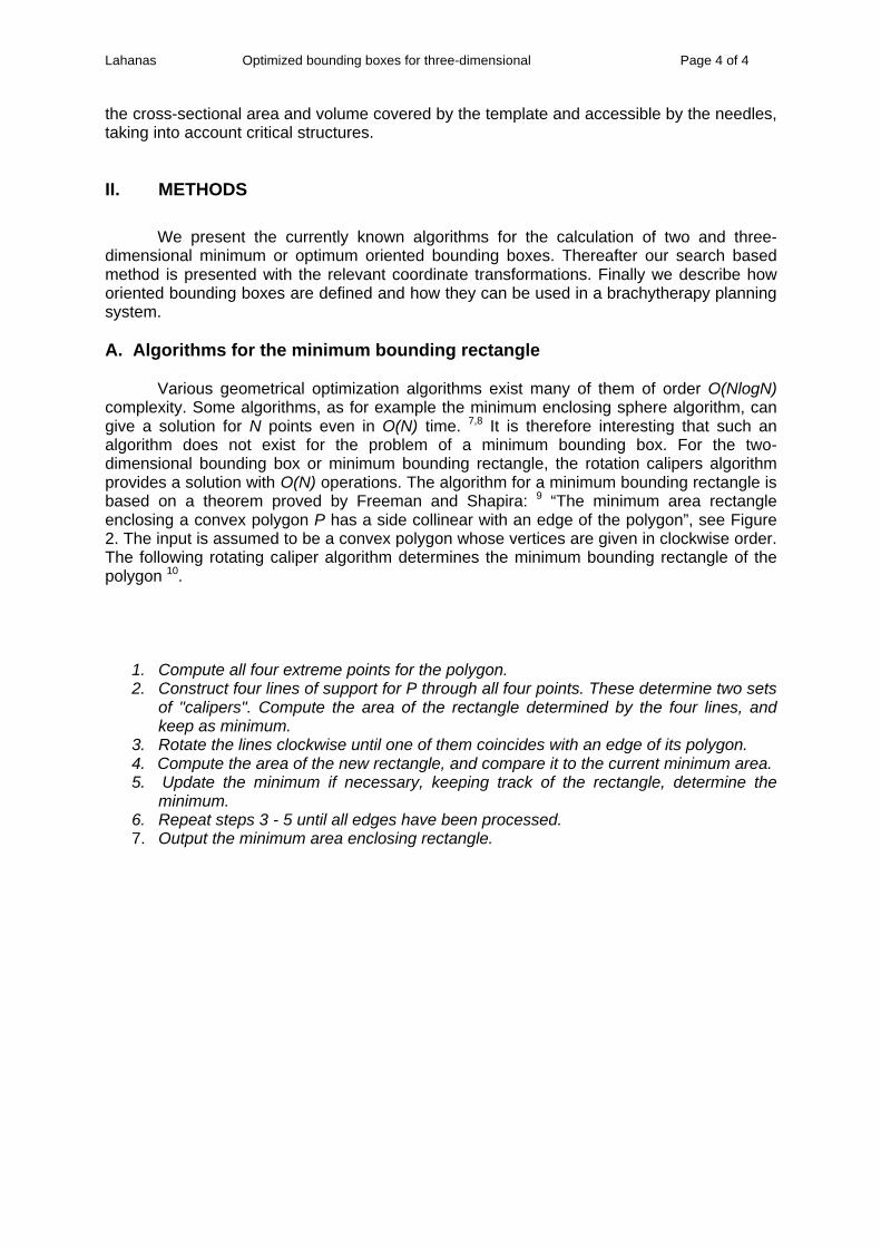
Various geometrical optimization algorithms exist many of them of order O(NlogN) complexity. Some algorithms, as for example the minimum enclosing sphere algorithm, can give a solution for N points even in O(N) time. 7,8 It is therefore interesting that such an algorithm does not exist for the problem of a minimum bounding box. For the two-dimensional bounding box or minimum bounding rectangle, the rotation calipers algorithm provides a solution with O(N) operations. The algorithm for a minimum bounding rectangle is based on a theorem proved by Freeman and Shapira: 9 “The minimum area rectangle enclosing a convex polygon P has a side collinear with an edge of the polygon”, see Figure 2. The input is assumed to be a convex polygon whose vertices are given in clockwise order. The following rotating caliper algorithm determines the minimum bounding rectangle of the polygon 10.

1. Compute all four extreme points for the polygon. 2. Construct four lines of support for P through all four points. These determine two sets

of "calipers". Compute the area of the rectangle determined by the four lines, and keep as minimum.

3. Rotate the lines clockwise until one of them coincides with an edge of its polygon. 4. Compute the area of the new rectangle, and compare it to the current minimum area. 5. Update the minimum if necessary, keeping track of the rectangle, determine the

minimum. 6. Repeat steps 3 - 5 until all edges have been processed. 7. Output the minimum area enclosing rectangle.

Lahanas Optimized bounding boxes for three-dimensional Page 5 of 5

B. Algorithms for the minimum bounding box

A variant of Freeman’s theorem for rectangles exists also for three-dimensional

bounding boxes: “A box of minimal volume enclosing a convex polyhedron must have at least two adjacent faces flush with edges of the polyhedron”. 9

The only exact algorithm due to O’Rourke for the calculation of a minimum bounding

box of a three-dimensional set of points is a rotating caliper variant in 3D. 11 This algorithm requires O(N3) operations for the determination of a minimum bounding box for N points. The number of vertices of objects in medical applications described by contours can exceed 1000 and therefore the number of operations required for the minimum bounding box is very large. Using the convex hull of the points can reduce this number, but not always by a very significant amount.

Recently two deterministic methods for an optimal oriented bounding box were

presented. 6 One method requires of the order O(N+ 1/ε4.5) operations whereas the running time of the other algorithm is O(NlogN + N/ε3). If Bopt is the minimum bounding box and V(Bopt) its volume, then the algorithms can be used for the calculation of a bounding box B with a volume V(B) so that V(B)< (1+ε)V(Bopt) where ε is the required accuracy. The first algorithm is claimed by its authors is to be difficult to implement. The second algorithm which was tested by the authors is a exhaustive grid based search algorithm which requires the calculation of some properties of the set of points such as the convex hull and some initial approximation of the minimum bounding box.

Lahanas Optimized bounding boxes for three-dimensional Page 6 of 6

1. Bounding box using the covariance matrix A more frequently used algorithm for the minimum bounding box of a set of points,

uses the covariance matrix of these points. If pi = (pix,piy,piz) is the ith point, then the center C of the set of N points is

and the covariance matrix C is:

Large valued non-diagonal covariance matrix elements in a coordinate system reveal that the object is not aligned with the coordinate system. In a coordinate system where the covariance matrix is diagonal it is expected that the corresponding bounding box will be close to the minimum bounding box. The eigenvectors of this matrix define the axes of the minimum bounding box and its dimensions. The eigenvectors can be obtained using the QL algorithm of Numerical Recipes. 5 A Householder transformation yields a tridiagonal matrix T from C. Since C is a real symmetric matrix a transformation exists so that T = QT⋅C⋅Q, where Q is a orthogonal matrix. The dimension of the bounding box along an axis (eigenvector) is given by the extreme values of the projection of the points on the corresponding axis.

We call V1 the volume of the bounding box obtained by the covariance matrix of the set of points. As the covariance matrix depends on the distribution of points there is not always a strong correlation between the eigenvectors and the main axes of the minimum bounding box such as in the case when a significant number of points is located in a small part of the space. Therefore to overcome this problem variants of the covariance matrix based method have been proposed. If a triangulation of its surface exists, then the covariance matrix obtained using all the surface points can be used. This can be achieved by replacing the summation over the contour points in Eq. (1) with an integration over all points of the triangulated surface. The resulting center of mass and the covariance matrix elements obtained from the integration over the triangulated surface is described in Appendix I. We call V2 the volume of the bounding box obtained by this approach.

A third variant proposed by Gottschalk et al. uses the covariance matrix obtained by

the triangulated convex hull of the points, see Appendix I. 12 We call V3 the volume of the bounding box obtained by this approach. Which of these methods is better can only be determined experimentally. In Fig. 3 we see an example of the bounding boxes obtained by these three variants for a rib implant.

(2) ))((1

1∑

=

−−=N

i

TiiN

cpcpC

(1) 1

1∑

=

=N

iiN

pC

Lahanas Optimized bounding boxes for three-dimensional Page 7 of 7

2. Bounding box using a search based optimization method We use another approach which overcomes the problems of the covariance based

method CM is easy to implement and does not require the computation of geometrical quantities such as the convex hulls and a specified approximate initial solution.

We use Powell’s quadratic convergent optimization method 5 for the search of an optimal oriented bounding box. Other optimization methods which do not require gradients of the objective function could be used, such as simulated annealing but we decided to use Powell’s method due to its simplicity.

We initialize the set of directions ui to the basis vectors ei. The goal of this optimization is to minimize the bounding box volume V obtained after rotation of the point set around an axis by some angle α. Given a direction u the angle which gives a minimum bounding volume along this direction can be determined. The optimization goal is a set of angles (ϕ, θ, α) which minimize V(ϕ, θ, α). VOpt is the bounding box volume obtained by this method.

Lahanas Optimized bounding boxes for three-dimensional Page 8 of 8

C. Searching an optimum of a direction dependent quantity.

We consider the problem of the determination of a direction vector u which optimizes some utility function f(u, ...), where f can depend on additional parameters some of which are direction dependent.

A rotation in n-dimensional space leaves invariant a n-2 dimensional subspace. In two

dimensions an invariant is a point, in three dimensional space a line is invariant after an arbitrary rotation etc. If we assume that the n-2 dimensional invariant space can be described by the n-2 basis vectors e1,…,en-2 then a rotation around an angle α can be described by a matrix

where P is a skew symmetric see Appendix II for details. In three-dimensional space the invariant can be viewed as a rotation axis u = (u1,u2,u3). Using spherical coordinates this vector u can be specified using the spherical angles (ϕ,θ) i.e. u = (u1,u2,u3) = (sin(θ)cos(ϕ), sin(θ)sin(ϕ), cos(θ)) and the utility function f depends on the three parameters (ϕ,θ,α). Given a direction u the angle which optimizes the utility function along this direction can be determined. We use Powell’s quadratic convergent method. 5 The search in the θ direction actually is a search in cosθ which ensures that the angular space is uniformly searched. In order to escape from local minima we introduced a grid search method using a multi-scale approach. From the current search position new directions specified by a grid of a specified size and a given grid size are searched for a possible better solution. If a better solution is found on one of these grid points, then the search is repeated on a grid in a smaller part of space with a smaller grid constant around the previously found minimum. This process is repeated a few times.

D. Application of optimal oriented bounding boxes 1. Production of points inside the optimized bounding box

Oriented bounding boxes are used to efficiently produce points inside objects, but

also they can be used to speed up the generation of sampling points in objects used eg. for the calculation of their volume using Monte-Carlo methods. The production of points inside the minimum bounding box will increase the efficiency of the procedure by reducing the probability of generating points outside the object. This effect becomes very significant if the main axes of the object are not aligned with the coordinate system in use.

An optimal oriented bounding box is specified by borig the origin of the oriented bounding box with respect to the coordinate system in use and the vectors b1, b2, b3 which define the main axes of the box, see Fig. 4. A point p inside this box can be generated by r1, r2, r3 ∈ [0, 1] can be either random or quasi-random numbers. 5

2. Test if a point is inside an optimized bounding box In some cases, such as the prostate, a critical structure, in this example the urethra,

is surrounded by the PTV volume giving a PTV that is not continuously filling the anatomical volume enclosed by the PTV outer contours. In such cases, points generated inside the 3D PTV contour surface must be ignored if they are within any critical structure. In addition, any points inside the PTV, critical structures and any tissue volume, which are also inside the

(3) ))cos(1()sin(),,...,,( 2221 PPeeeR n ⋅−+⋅+=− ααα 1

(4) r r r 332211orig bbbbp +++=

Lahanas Optimized bounding boxes for three-dimensional Page 9 of 9

catheters, should be ignored. This can be done efficiently if oriented bounding boxes of the catheters and anatomical structures is used. The test of whether a point is inside an oriented bounding box can be made solving the linear equation system defined by Eq. (4) using Cramer’s Rule with unknowns r1, r2, r3. If r1, r2, r3 ∈ [0, 1] then the point is inside the oriented bounding box. 3. Expanding an optimum oriented bounding box

An expanded version of an optimum oriented bounding box can be used to cover the PTV and a surrounding region efficiently for anatomy based optimization methods which define a region called “the body”. This is required for the following.

1) Production of sampling points using a stratified sampling method for dose

calculation in regions, where the regions are optimum oriented bounding boxes or minimum enclosing spheres.

2) For optimum oriented dose calculation grids which include the PTV and surrounding tissue for FFT based methods for the calculation of the dose distribution 3,4 or other methods which require the dose to be known on grid points such as for isodose drawing algorithms.

If lb1, lb2, lb3 is the required offset of the expanded oriented bounding box in each direction the corresponding relative increase of the length of the vector b1 e.g. is The resulting vectors of the expanded bounding boxes b1’, b2’ and b3’ are obtained from a scaling of the original bounding box vectors The new origin b’orig of the expanded bounding box, see Figure 5, is then: 4. Optimal oriented dose calculation grid

Optimal oriented bounding boxes can be used to improve the performance and accuracy of the FFT based method for the computation of the dose distribution as described by Boyer et al. 3 Usually the FFT method uses a three-dimensional grid which is oriented with respect to the coordinate system in use. If the anatomical structure is not oriented to this structure then the number of grid points inside the anatomical structure can be small compared to the total number of grid points. If we orient the grid system so that the oriented bounding box volume in this system is minimal we maximize the number of grid points which will be inside the anatomical structure, see Fig. 6.

1b1bl=α

33

22

11

bbbbbb

)21(')21(')21('

γβα

+=+=+=

z

y

x

z

y

x

z

y

x

zorig

yorig

xorig

zorig

yorig

xorig

bbb

bbb

bbb

bbb

bbb

3

3

3

2

2

2

1

1

1

'''

γγγ

βββ

ααα

−−−

−−−

−−−

===

Lahanas Optimized bounding boxes for three-dimensional Page 10 of 10

The benefit of using an optimal oriented grid is shown in Fig. 7 for the distribution of

the shifts of the sources to the closest grid points using the original grid and an optimal oriented dose calculation grid. Not only the width but also the mean shift has been reduced. An additional benefit is an increase of the number of grid points inside the PTV for a fixed total number of grid points. In comparison to the original grid the increase of grid points using an optimal oriented grid can be from a few percent to greater than 100 percent for elongated objects.

Lahanas Optimized bounding boxes for three-dimensional Page 11 of 11

5. Use of optimum oriented bounding boxes for DVH computation using stratified sampling

We use optimum oriented bounding boxes for the calculation of DVHs. In our anatomy based optimization algorithm the optimization is based on the conformity index COIN derived from the DVHs of the body and the PTV. 1 A conventional method calculating the DVH for the body using uniform distributed sampling points would require a very large number of sampling points if a sufficiently large part of tissue surrounding the PTV has to be considered.

We therefore developed a method which is partly based on the stratified sampling technique in Monte Carlo integration in which the region of interest is divided in regions (strata) with different but uniform sampling point density. 5 These strata are the PTV and two expanded optimal oriented bounding boxes of the PTV or an expanded bounding box and a sphere, which defines the body. These are used to define regions of very high, high and low dose gradients. The use of oriented bounding boxes increases the efficiency of this method as they cover more efficiently the PTV and the surrounding tissue.

As a result we show the accuracy of the DVH of the body for a rib implant with 10000 sampling points uniformly distributed inside the body obtained by a conventional method compared to a very high statistics DVH obtained with 3 000 000 sampling points, see Fig. 8(a). The corresponding accuracy as a function of total 10000 sampling points distributed in the strata is shown in Fig. 8(b). The accuracy of the stratified sampling method is significantly higher even at high dose values.

Lahanas Optimized bounding boxes for three-dimensional Page 12 of 12

III. MATERIAL

We first compared all the covariance matrix based variants with our search based method. This is to determine whether the former gives sufficiently good results. The material used in this study include 10 actual clinical implants which represent a typical range of PTVs from 20 cm3 to 500 cm3 which are encountered in clinical practice. We compare the original bounding box volume with the bounding box volume obtained from the three variants of the covariance matrix method and with our search based algorithm. We also include the tightness factor for the original and the optimized bounding box obtained by our method. This factor is defined as the ratio of the bounding box volume to the volume of the object it encloses.

Since the actual minimum bounding box volume for the implants is not known we

used a test set of points with a known minimum bounding box. The test cases are generated using a point on each corner of a bounding box, and include a variable number of additional points inside this box. The coordinates are transformed using a random rotation matrix which simulates a random orientation of the bounding box. The optimization algorithm is then applied with the transformed coordinates. The result of the optimization is shown in Table 1. We used bounding boxes with sides 1/1/1, 1/1/2, 1/1/5 and 1/1/10, which cover a range of dimensions of objects typically found in brachytherapy clinical practice. IV. RESULTS

Table 1 shows the volume of the bounding box for objects in 10 implants. The volume

of the bounding box obtained by various covariance matrix methods are compared with the result of our orientation search based method including the volume of the original bounding box. If the objects are not aligned with the coordinate system in use then the bounding box volume from the covariance method results in an improved bounding volume, otherwise the result can be significantly worse than the original bounding volume. This shows that the covariance matrix based method is of limited practical use. Our orientation search method always resulted in a better solution. For the PTV and critical structures the average tightness factor was improved from 4.4 to 2.6.

Fig. 9 shows the time which is required for the algorithm to produce the resulting

optimum oriented bounding box. This time is averaged over 1000 runs for the most elongated box with sides 1/1/10 as a function of the number of points which define the box. Linear dependence is observed in Figure 9. These results have been obtained using a 400 MHz Intel Pentium II system with Windows 98. Tests have shown that the time is approximately independent on the shape of the box.

The accuracy of our method has been tested with boxes of known sizes with a ratio

of sides from 1/1/1, 1/1/2, 1/1/5 to 1/1/10. We consider the true bounding box volume of the object Vmin, the volume Vopt which is obtained from our search method and Vorig the bounding box volume in the world coordinate system after a random rotation has been applied to all points of the set. In Fig. 10 we have compared the distribution of the optimized bounding box volume to the true volume with the non-optimized ratio from the arbitrary oriented boxes as obtained from 1000 runs.

In Table II the average values of these ratios and the maximum value observed for the optimized and the arbitrary oriented box is given.

Lahanas Optimized bounding boxes for three-dimensional Page 13 of 13

V. CONCLUSIONS A method for the search of a optimal direction has been introduced and its application

for the bounding box optimization of a set of points has been presented. The covariance matrix based methods have been shown to fail to produce good solutions for most cases. Our search based method produces results close to the true minimum. The time is proportional to the number of points which define the minimum bounding box.

The minimum bounding box algorithm has several applications in the field of

brachytherapy treatment planning. The calculation of bounding boxes for catheters, the PTV and other anatomical structures requires only 2-3 seconds on the average which is much less than the time saved by a more efficient volume and DVHs calculation. Our results present some of the benefits of the use of minimum bounding boxes in brachytherapy.

Lahanas Optimized bounding boxes for three-dimensional Page 14 of 14

( ) (I.2) 3/321iiii vvvc ++=

APPENDIX I Calculation of the covariance matrix of a triangulated surface

The center of gravity c of a 3D triangulated surface F is given by:

where r is a point lying on the triangulated surface and ρ(r) is the surface density which we assume to be constant. Given the ith triangle with vertices vi

1, vi2, vi

3 the center of gravity of the ith triangle ci

. is

The contributions of each triangle to the center of the triangulated surface is proportional to its area. Therefore the center of gravity c of the triangulated surface is given by

where Fi is the area of the ith triangle.

The covariance matrix C of a surface F is given by:

where r is a point lying on the surface and ρ(r) is the surface density which we assume to be constant. The contribution of the ith triangle to the covariance matrix Ci is given by:

where the point r is expressed using barycentric coordinates s,t. 2

( )

( )(I.1)

∫

∫=

F

F

dF

dF

r

rrc

ρ

ρ

( )

( )(I.4)

))((

∫

∫ −−=

F

F

T

dF

dF

r

rcrcrC

ρ

ρ

(I.5) )),()(),((

1

0

1

0

1

0

1

0

∫ ∫

∫ ∫−

−

−−= t

tTii

i

dsdt

dsdttsts crcrC

(I.3) N

1i/

N

1i31 TT

∑=

∑=

= iii FF cc

Lahanas Optimized bounding boxes for three-dimensional Page 15 of 15

After the integration of Eq. (I.5) we obtain Eq. (I.6).

The covariance matrix C of the triangulated surface is given by

(I.7) /11

∑∑==

=N

i

iN

i

ii FF CC

(I.6) )])(())(([241 3

1

3

1

3

1ββααββαααβ cvcvcvcv k

ik

i

kk

i

j kj

ii −−+−−= ∑∑∑== =

C

Lahanas Optimized bounding boxes for three-dimensional Page 16 of 16

APPENDIX II

Transformation matrix for a rotation around an arbitrary three-dimensional vector

Given an axis u = (u1,u2,u3) then a rotation of a vector w around this axis by an angle

α can be described by the transformation matrix R, see Fig 11(a),

where ⊗ denotes the tensor product. Eq. (II.1) is equivalent with Eq. (3), with matrix elements

P is a skew symmetric matrix formed by the elements of u, called the dual to u matrix. δij is the Kronecker delta symbol and εijk the anti-symmetric permutation tensor.

The angle α and the rotation axis u can be obtained from the trace of R and its transposed matrix RT using the Equations (II.5) and (II.6).

Fig. 11(b) shows the derivation of Equation (II.1). We consider the components of w parallel and perpendicular to u, w|| and wT respectively. The term u⊗u = uuT describes the projection w|| of w onto u which remains unchanged after a rotation around u. (1-uuT) describes the projection of w onto the plane on which u is perpendicular and P describes a projection of w onto the plane where u’s is normal. This operation is followed by an additional rotation by an angle π/2.

II.3)( 0

00

12

13

23

−−

−=

uuuu

uuP

(II.6) )sin(2 TRRP −=α

(II.4) ∑=k

kijkij uP ε

−=

else0 npermutatio oddan is )( if1npermutatioeven an is )( if 1

ijkijk

ijkε

(II.1) sincos)( αα Puu1uuR +⊗−+⊗=

(II.2) sincos)( ∑+−+=k

kijkjiijjiij uuuuuR εααδ

[ ] (II.5) 1)(21

)cos( −= Rtraceα

Lahanas Optimized bounding boxes for three-dimensional Page 17 of 17

Given a transformation matrix R we can determine the corresponding rotation axis u from P using Eq. (II.6), whereas the corresponding rotation angle is given by Equation (II.5). If R-RT = 0 then the rotation angle is 0 or π and the rotation axis can be obtained from R. In this case it follows that R has as diagonal matrix elements the following:

(II.7) 1)- 2u 1,- 2u 1,- diag(2u 23

22

21

Lahanas Optimized bounding boxes for three-dimensional Page 18 of 18

VI. REFERENCES 1M. Lahanas, D. Baltas and N. Zamboglou, “Anatomy-based three-dimensional dose optimization in brachytherapy using multiobjective genetic algorithms,'' Med. Phys. 26, 1904-1918 (1999). 2M. Lahanas, D. Baltas, S. Giannouli, N. Milickovic, and N. Zamboglou, “Generation of uniformly distributed dose points for anatomy-based three-dimensional dose optimization methods in brachytherapy,” to appear in Med. Phys. 27 (2000). 3A. L. Boyer, E. C. Mok, “Brachytherapy seed dose distribution calculation employing the fast Fourier transform,” Med. Phys 13, 525-529 (1986). 4T. Kemmerer, M. Lahanas, D. Baltas and N. Zamboglou, “Comparison of DVHs computation in brachytherapy using conventional methods and optimized FFT algorithms,” submitted for publication in Medical Physics. 5W. H. Press, S. A. Teukolsky, W.T. Vetterling, B. P. Flannery, Numerical Recipes in C, 2nd ed. (Cambridge University Press, Cambridge, 1992). 6G. Barequet and S. Har-Peled, Efficiently approximating the minimum-volume bounding box of a point set in three dimensions, Proc. 10th Ann. ACM-SIAM Symp. On Discrete Algorithms (SODA), Baltimore, MD, pp. 82-91, January 1999. 7Welzl Emo, Smallest enclosing disks (balls and ellipsoids): In H. Maurer, editor, New Results and New Trends in Computer Science, volume 555 of Lecture Notes in Computer Science 359-370. Springer-Verlag, 1991. 8B. Gärnter, Fast and robust smallest enclosing balls., Proc. 7th Annual European Symposium on Algorithms (ESA), Lecture Notes in Computer Science 1643, Springer Verlag, pp. 325-338 (1999). 9H. Freeman and R. Shapira, “Determining the minimum-area encasing rectangle for an arbitrary closed curve,” Commun. of the ACM. 18, 409-413 (1975). 10G. T. Toussaint. “Solving geometric problems with the rotating calipers”. In Proc. IEEE MELECON, Athens, pages A10.02/1-4, 1983. 11J. O.‘ Rourke. ,”Finding minimal enclosing boxes,“ Internat. J. Comput. Inform. Sci. 14, 183-199, June 1985. 12S. Gottschalk, M. Lin and D. Manocha, “Obb-tree: A hierarchical structure for rapid interference detection,” In Proc. of ACM Siggraph‘1996, 171-180 (1996).

Lahanas Optimized bounding boxes for three-dimensional Page 19 of 19

Figure Legends Figure 1. Contours of a critical structure (myelon) and the catheters of an implant showing the original bounding box (white) and the optimized bounding box (red).

Figure 2. A minimum bounding rectangle defined by six points using the rotating calipers algorithm. A side of the convex hull of the points must be collinear with one side of the minimum bounding rectangle, such as the side 2-3.

Figure 3. Optimum bounding box of a rib implant obtained by the covariance matrix method. (a) using the contour points, (b) using the triangulated convex hull and (c) using the triangulated surface.

Figure 4. Production of a point P inside a oriented bounding box. The four vectors borig, b1, b2 and b3 are used to define a oriented bounding box with respect to a global coordinate system with the unit basis vectors e1, e2 and e3. Figure 5. A oriented bounding box expanded by Ib1, lb2 and lb3 units of length in the direction specified respectively by b1, b2 and b3. The centers of the original and expanded box are the same. Figure 6. (a) Original and (b) optimal oriented dose calculation grid for a rib implant, produced inside the original and optimal oriented bounding boxes respectively. The number of sampling points in both cases is the same. Figure 7. Distribution of the shift ∆ of the source dwell positions from their original positions to the closest situated grid point using (a) the original 16×16×32 grid and (b) the optimal oriented 16×32×16 dose calculation grid for a rib implant, see Fig. 6. Figure 8. Accuracy of the DVH of the body of a 500 cm3 large rib implant in comparison to a high statistics reference distribution using (a) the conventional and (b) the stratified sampling method. The volume of the Body which surrounds and includes the PTV is 4400 cm3. Figure 9. Calculation time averaged over 1000 random oriented sets of points for our optimal oriented bounding box algorithm which is a function of the number of points with the standard deviation for a box having a ratio of sides 1/2/5. For 500 and 2000 points the average calculation time for a box with sides 1/1/10 is included. Figure 10. Distribution of the ratio a=Vorig/Vmin. This is the ratio for the original box to the minimum bounding box volume using arbitrary oriented sample of points. The ratio b=Vopt/Vmin is also shown for the optimized to the minimum bounding box volume (a) for a box with sides 1/1/1 (b) with sides 1/1/2 (c) with sides 1/1/5 and (d) with sides 1/1/10. Figure 11. (a) Rotation of a vector w around an arbitrary axis u by an angle α. (b) components of w in the plane which is perpendicular to the rotation axis u after the rotation.

TABLES

Object No.

Implant Description Vorig

cm3

V1

cm3

V2

cm3

V3

cm3

Vopt

cm3

Vobj

cm3

Original tightness factor T1

Optimized tightness factor T2

T1/T2

1 PTV 402.07 440.15 447.99 447.26 381.30 152.22 2.64 2.50 1.05

2

Head & Neck

Myelon 98.57 36.52 35.57 33.99 32.99 13.85 7.12 2.38 2.99

3 Breast PTV 278.47 350.66 362.55 347.26 228.40 121.91 2.28 1.87 1.22

4 PTV 120.83 151.21 157.99 157.83 119.30 62.20 1.94 1.91 1.01

5 Urethra 4.41 2.46 2.43 2.42 2.38 0.59 7.47 4.03 1.85

6

Prostate

Rectum 77.62 122.20 124.99 99.59 72.16 31.43 2.47 2.30 1.08

7 Cervix PTV 1001.70 1090.54 1140.49 1037.73 915.78 291.00 3.44 3.15 1.09

8 Breast PTV 59.62 54.28 54.45 53.02 49.69 18.41 3.24 2.70 1.20

9 PTV 47.51 54.35 55.37 56.72 44.92 20.79 2.29 2.16 1.06

10 Urethra 4.38 1.55 1.67 1.60 1.47 0.28 15.64 5.25 2.98

11

Prostate

Rectum 137.73 168.17 170.82 164.79 132.27 46.77 2.94 2.83 1.04

12 PTV 2410.85 1554.40 1733.64 1505.84 1338.50 504.04 4.78 2.66 1.80

13

Rib

Left kidney 643.01 662.95 663.79 670.23 595.86 236.60 2.72 2.52 1.08

14 Breast PTV 266.44 279.52 281.16 286.72 247.14 123.11 2.16 2.01 1.08

15 Head & Neck PTV 49.06 47.30 47.57 49.11 39.55 17.72 2.77 2.23 1.24

Lahanas Optimized bounding boxes for three-dimensional Page 22 of 22

16 PTV 43.86 53.20 59.24 56.14 43.86 21.63 2.03 2.03 1

17 Urethra 5.94 1.68 1.66 1.76 1.46 0.54 11.0 2.70 4.07

18

Prostate

Rectum 54.93 66.23 68.59 74.30 53.62 23.08 2.38 2.32 1.02

TABLE I. Volume results of different minimum bounding box approximation methods V1, V2, V3 and Vopt used in this study. The tightness factor is defined in the text.

Ratio of box sides Non-optimized bounding box Optimized bounding box

Lx/Ly/Lz Mean(Vorig/Vmin) Max(Vorig/Vmin) Mean(Vopt/Vmin) Max(Vopt/Vmin) 1/1/1 2.78 ±0.98 4.61 1.01±0.09 2.00 1/1/2 3.15 ±1.21 5.48 1.03±0.12 2.00 1/1/5 5.69 ±3.00 12.25 1.08±0.22 2.65 1/1/10 12.32 ±8.24 31.82 1.23±0.35 4.09 TABLE II. Comparison of volume ratios for the optimized and non-optimized oriented bounding boxes to the true volumes of the boxes.

M. Lahanas, T. Kemmerer et al. Geometric optimization of the bounding box.. Page 24 of 24

M. Lahanas et al. Figure 1.

M. Lahanas, T. Kemmerer et al. Geometric optimization of the bounding box.. Page 25 of 25

M. Lahanas et al. Figure 2.

Minimum bounding rectangle

Original bounding rectangle

1 6

54

3

2

M. Lahanas, T. Kemmerer et al. Geometric optimization of the bounding box.. Page 26 of 26

M. Lahanas et al. Figure 3(a).

M. Lahanas, T. Kemmerer et al. Geometric optimization of the bounding box.. Page 27 of 27

M. Lahanas et al. Figure 3(b).

M. Lahanas, T. Kemmerer et al. Geometric optimization of the bounding box.. Page 28 of 28

M. Lahanas et al. Figure 3(c).

M. Lahanas, T. Kemmerer et al. Geometric optimization of the bounding box.. Page 29 of 29

M. Lahanas et al. Figure 4.

P

b1

b2 b3

e1

e2

e3 borig

M. Lahanas, T. Kemmerer et al. Geometric optimization of the bounding box.. Page 30 of 30

M. Lahanas et al. Figure 5.

M. Lahanas, T. Kemmerer et al. Geometric optimization of the bounding box.. Page 31 of 31

M. Lahanas et al. Figure 6(a).

M. Lahanas, T. Kemmerer et al. Geometric optimization of the bounding box.. Page 32 of 32

M. Lahanas et al. Figure 6(b).

M. Lahanas, T. Kemmerer et al. Geometric optimization of the bounding box.. Page 33 of 33

M. Lahanas et al. Figure 7(a).

0 1 2 3 4 5 60

5

10

15

20

25

30

35

∆ [mm]

dN/d

∆

M. Lahanas, T. Kemmerer et al. Geometric optimization of the bounding box.. Page 34 of 34

M. Lahanas et al. Figure 7(b).

0 1 2 3 4 5 60

10

20

30

40

50

dN/d

∆

∆ [mm]

M. Lahanas, T. Kemmerer et al. Geometric optimization of the bounding box.. Page 35 of 35

M. Lahanas et al. Figure 8(a).

0 2 4 6 8 10-40

-30

-20

-10

0

10

20

30

40 BODY

Ac

cu

rac

y (

%)

D /Dref

Conventional

N=10000

M. Lahanas, T. Kemmerer et al. Geometric optimization of the bounding box.. Page 36 of 36

M. Lahanas et al. Figure 8(b).

0 2 4 6 8 10-40

-30

-20

-10

0

10

20

30

40BODY Stratified Sampling

D/Dref

Ac

cu

rac

y (

%)

N=10000

M. Lahanas, T. Kemmerer et al. Geometric optimization of the bounding box.. Page 37 of 37

M. Lahanas et al. Figure 9.

500 1000 1500 20000.0

0.5

1.0

1.5

2.0t [

sec]

N

1/2/5 1/1/10

M. Lahanas, T. Kemmerer et al. Geometric optimization of the bounding box.. Page 38 of 38

M. Lahanas et al. Figure 10(a).

0 1 2 3 4 5 60.1

1

10

1001/1/1

dn/d

a

a=Vorig

/Vmin

0 1 2 3 4 5 6

10

100

10001/1/1

dn/d

bb = V

opt/V

min

M. Lahanas, T. Kemmerer et al. Geometric optimization of the bounding box.. Page 39 of 39

M. Lahanas et al. Figure 10(b).

0 1 2 3 4 5 6

10

100

1000

1/1/2

dn/d

bb = V

opt/V

min

0 1 2 3 4 5 6

1

10

dn

/da

a=Vorig

/Vmin

1/1/2

M. Lahanas, T. Kemmerer et al. Geometric optimization of the bounding box.. Page 40 of 40

M. Lahanas et al. Figure 10(c).

0 2 4 6 8 10 12 141

10

100

1000

dn

/db

b = Vopt

/Vmin

1/1/5

0 2 4 6 8 10 12 140.1

1

10

1/1/5

dn/d

a

a=Vorig

/Vmin

M. Lahanas, T. Kemmerer et al. Geometric optimization of the bounding box.. Page 41 of 41

M. Lahanas et al. Figure 10(d).

0 5 10 15 20 25 30 351

10

100

1000

dn/d

b

b = Vopt

/Vmin

1/1/10

0 5 10 15 20 25 30 35

1

10

100

a=Vorig

/Vmin

dn/d

a

1/1/10

M. Lahanas, T. Kemmerer et al. Geometric optimization of the bounding box.. Page 42 of 42

M. Lahanas et al. Figure 11(a).

vT

w|| w

u

u wx

w⊥

Plane ⊥ u

α

M. Lahanas, T. Kemmerer et al. Geometric optimization of the bounding box.. Page 43 of 43

M. Lahanas et al. Figure 11(b).

w⊥ αcos

sinw⊥ α

In Plane u⊥

α

w⊥

u wx

w⊥

M. Lahanas, T. Kemmerer et al. Geometric optimization of the bounding box.. Page 44 of 44