Accurate 3D Bounding Box Estimation with Multi-Radars - arXiv
14
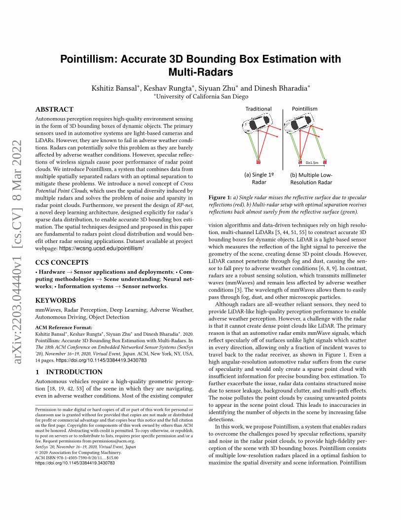
Pointillism: Accurate 3D Bounding Box Estimation with Multi-Radars Kshitiz Bansal ∗ , Keshav Rungta ∗ , Siyuan Zhu ∗ and Dinesh Bharadia ∗ ∗ University of California San Diego ABSTRACT Autonomous perception requires high-quality environment sensing in the form of 3D bounding boxes of dynamic objects. The primary sensors used in automotive systems are light-based cameras and LiDARs. However, they are known to fail in adverse weather condi- tions. Radars can potentially solve this problem as they are barely affected by adverse weather conditions. However, specular reflec- tions of wireless signals cause poor performance of radar point clouds. We introduce Pointillism, a system that combines data from multiple spatially separated radars with an optimal separation to mitigate these problems. We introduce a novel concept of Cross Potential Point Clouds, which uses the spatial diversity induced by multiple radars and solves the problem of noise and sparsity in radar point clouds. Furthermore, we present the design of RP-net, a novel deep learning architecture, designed explicitly for radar’s sparse data distribution, to enable accurate 3D bounding box esti- mation. The spatial techniques designed and proposed in this paper are fundamental to radars point cloud distribution and would ben- efit other radar sensing applications. Dataset available at project webpage: https://wcsng.ucsd.edu/pointillism/ CCS CONCEPTS • Hardware → Sensor applications and deployments; • Com- puting methodologies → Scene understanding; Neural net- works;• Information systems → Sensor networks. KEYWORDS mmWaves, Radar Perception, Deep Learning, Adverse Weather, Autonomous Driving, Object Detection ACM Reference Format: Kshitiz Bansal ∗ , Keshav Rungta ∗ , Siyuan Zhu ∗ and Dinesh Bharadia ∗ . 2020. Pointillism: Accurate 3D Bounding Box Estimation with Multi-Radars. In The 18th ACM Conference on Embedded Networked Sensor Systems (SenSys ’20), November 16–19, 2020, Virtual Event, Japan. ACM, New York, NY, USA, 14 pages. https://doi.org/10.1145/3384419.3430783 1 INTRODUCTION Autonomous vehicles require a high-quality geometric percep- tion [18, 19, 42, 53] of the scene in which they are navigating, even in adverse weather conditions. Most of the existing computer Permission to make digital or hard copies of all or part of this work for personal or classroom use is granted without fee provided that copies are not made or distributed for profit or commercial advantage and that copies bear this notice and the full citation on the first page. Copyrights for components of this work owned by others than ACM must be honored. Abstracting with credit is permitted. To copy otherwise, or republish, to post on servers or to redistribute to lists, requires prior specific permission and/or a fee. Request permissions from [email protected]. SenSys ’20, November 16–19, 2020, Virtual Event, Japan © 2020 Association for Computing Machinery. ACM ISBN 978-1-4503-7590-0/20/11. . . $15.00 https://doi.org/10.1145/3384419.3430783 (a) Single 1º Radar (b) Multiple Low- Resolution Radar D≥1.5m Pointillism Traditional Figure 1: a) Single radar misses the reflective surface due to specular reflections (red). b) Multi-radar setup with optimal separation receives reflections back almost surely from the reflective surface (green). vision algorithms and data-driven techniques rely on high resolu- tion, multi-channel LiDARs [5, 44, 51, 55] to construct accurate 3D bounding boxes for dynamic objects. LiDAR is a light-based sensor which measures the reflection of the light signal to perceive the geometry of the scene, creating dense 3D point clouds. However, LiDAR cannot penetrate through fog and dust, causing the sen- sor to fall prey to adverse weather conditions [6, 8, 9]. In contrast, radars are a robust sensing solution, which transmits millimeter waves (mmWaves) and remain less affected by adverse weather conditions [3]. The wavelength of mmWaves allows them to easily pass through fog, dust, and other microscopic particles. Although radars are all-weather reliant sensors, they need to provide LiDAR-like high-quality perception performance to enable adverse weather perception. However, a challenge with the radar is that it cannot create dense point clouds like LiDAR. The primary reason is that an automotive radar emits mmWave signals, which reflect specularly off of surfaces unlike light signals which scatter in every direction, allowing only a fraction of incident waves to travel back to the radar receiver, as shown in Figure 1. Even a high angular-resolution automotive radar suffers from the curse of specularity and would only create a sparse point cloud with insufficient information for precise bounding box estimation. To further exacerbate the issue, radar data contains structured noise due to sensor leakage, background clutter, and multi-path effects. The noise pollutes the point clouds by causing unwanted points to appear in the scene point cloud. This leads to inaccuracies in identifying the number of objects in the scene by increasing false detections. In this work, we propose Pointillism, a system that enables radars to overcome the challenges posed by specular reflections, sparsity and noise in the radar point clouds, to provide high-fidelity per- ception of the scene with 3D bounding boxes. Pointillism consists of multiple low-resolution radars placed in a optimal fashion to maximize the spatial diversity and scene information. Pointillism arXiv:2203.04440v1 [cs.CV] 8 Mar 2022
-
Upload
khangminh22 -
Category
Documents
-
view
1 -
download
0
Transcript of Accurate 3D Bounding Box Estimation with Multi-Radars - arXiv
Pointillism: Accurate 3D Bounding Box Estimation withMulti-Radars
Kshitiz Bansal∗, Keshav Rungta
∗, Siyuan Zhu
∗and Dinesh Bharadia
∗∗University of California San Diego
ABSTRACTAutonomous perception requires high-quality environment sensing
in the form of 3D bounding boxes of dynamic objects. The primary
sensors used in automotive systems are light-based cameras and
LiDARs. However, they are known to fail in adverse weather condi-
tions. Radars can potentially solve this problem as they are barely
affected by adverse weather conditions. However, specular reflec-
tions of wireless signals cause poor performance of radar point
clouds. We introduce Pointillism, a system that combines data from
multiple spatially separated radars with an optimal separation to
mitigate these problems. We introduce a novel concept of CrossPotential Point Clouds, which uses the spatial diversity induced by
multiple radars and solves the problem of noise and sparsity in
radar point clouds. Furthermore, we present the design of RP-net,a novel deep learning architecture, designed explicitly for radar’s
sparse data distribution, to enable accurate 3D bounding box esti-
mation. The spatial techniques designed and proposed in this paper
are fundamental to radars point cloud distribution and would ben-
efit other radar sensing applications. Dataset available at project
webpage: https://wcsng.ucsd.edu/pointillism/
CCS CONCEPTS•Hardware → Sensor applications and deployments; • Com-puting methodologies → Scene understanding; Neural net-works; • Information systems → Sensor networks.
KEYWORDSmmWaves, Radar Perception, Deep Learning, Adverse Weather,
Autonomous Driving, Object Detection
ACM Reference Format:Kshitiz Bansal
∗, Keshav Rungta
∗, Siyuan Zhu
∗and Dinesh Bharadia
∗. 2020.
Pointillism: Accurate 3D Bounding Box Estimation with Multi-Radars. In
The 18th ACM Conference on Embedded Networked Sensor Systems (SenSys’20), November 16–19, 2020, Virtual Event, Japan. ACM, New York, NY, USA,
14 pages. https://doi.org/10.1145/3384419.3430783
1 INTRODUCTIONAutonomous vehicles require a high-quality geometric percep-
tion [18, 19, 42, 53] of the scene in which they are navigating,
even in adverse weather conditions. Most of the existing computer
Permission to make digital or hard copies of all or part of this work for personal or
classroom use is granted without fee provided that copies are not made or distributed
for profit or commercial advantage and that copies bear this notice and the full citation
on the first page. Copyrights for components of this work owned by others than ACM
must be honored. Abstracting with credit is permitted. To copy otherwise, or republish,
to post on servers or to redistribute to lists, requires prior specific permission and/or a
fee. Request permissions from [email protected].
SenSys ’20, November 16–19, 2020, Virtual Event, Japan© 2020 Association for Computing Machinery.
ACM ISBN 978-1-4503-7590-0/20/11. . . $15.00
https://doi.org/10.1145/3384419.3430783
(a) Single 1º Radar
(b) Multiple Low-Resolution Radar
D≥1.5m
PointillismTraditional
Figure 1: a) Single radar misses the reflective surface due to specularreflections (red). b) Multi-radar setup with optimal separation receivesreflections back almost surely from the reflective surface (green).
vision algorithms and data-driven techniques rely on high resolu-
tion, multi-channel LiDARs [5, 44, 51, 55] to construct accurate 3D
bounding boxes for dynamic objects. LiDAR is a light-based sensor
which measures the reflection of the light signal to perceive the
geometry of the scene, creating dense 3D point clouds. However,
LiDAR cannot penetrate through fog and dust, causing the sen-
sor to fall prey to adverse weather conditions [6, 8, 9]. In contrast,
radars are a robust sensing solution, which transmits millimeter
waves (mmWaves) and remain less affected by adverse weather
conditions [3]. The wavelength of mmWaves allows them to easily
pass through fog, dust, and other microscopic particles.
Although radars are all-weather reliant sensors, they need to
provide LiDAR-like high-quality perception performance to enable
adverse weather perception. However, a challenge with the radar
is that it cannot create dense point clouds like LiDAR. The primary
reason is that an automotive radar emits mmWave signals, which
reflect specularly off of surfaces unlike light signals which scatter
in every direction, allowing only a fraction of incident waves to
travel back to the radar receiver, as shown in Figure 1. Even a
high angular-resolution automotive radar suffers from the curse
of specularity and would only create a sparse point cloud with
insufficient information for precise bounding box estimation. To
further exacerbate the issue, radar data contains structured noise
due to sensor leakage, background clutter, and multi-path effects.
The noise pollutes the point clouds by causing unwanted points
to appear in the scene point cloud. This leads to inaccuracies in
identifying the number of objects in the scene by increasing false
detections.
In this work, we propose Pointillism, a system that enables radars
to overcome the challenges posed by specular reflections, sparsity
and noise in the radar point clouds, to provide high-fidelity per-
ception of the scene with 3D bounding boxes. Pointillism consists
of multiple low-resolution radars placed in a optimal fashion to
maximize the spatial diversity and scene information. Pointillism
arX
iv:2
203.
0444
0v1
[cs
.CV
] 8
Mar
202
2
SenSys ’20, November 16–19, 2020, Virtual Event, Japan K. Bansal, K. Rungta, S. Zhu, D. Bharadia
combines this spatial diversity with novel multi-radar fusion algo-
rithms to tackle the problem of specular reflections, sparsity and
noise in radar point clouds. Building upon the hardware and algo-
rithms, Pointillism also introduces a novel data-driven approach
that enables the detection of multiple dynamic objects in the scene,
with their accurate location, orientation and 3D dimensions. Fur-
thermore, Pointillism enables such perception even in inclement
weather, thereby paving a way for radar to be the main-stream
sensor for autonomous perception.
A natural question is how does Pointillism overcomes the physics
of wireless signals i.e., specularity. Pointillism’s key idea to over-
come specular reflections is to use multiple radars placed at spatially
separated locations overlooking the same scene and illuminate an
object in the scene from different viewpoints. This, in turn, in-
creases the probability of receiving a reflection back from multiple
points/surfaces of the object, which single radar could have missed,
as shown in Figure 1. Pointillism formulates the problem of optimal
placement of multiple low-resolution radars as an optimization
problem to achieve multiple reflection points from a vehicle at all
orientation. The optimization reveals that the optimal radar place-
ment of around 1.5 meter apart (typical width of a car) to achieve
high-fidelity in the estimated pose of the surface.
A good placement ensures spatial diversity in the point clouds,
but noise is still a major challenge. Pointillism presents a novel
multi-radar fusion algorithm that reduces the noise points to enable
accurate detection of multiple dynamic objects. The insight is to
use spatial diversity generated by multiple radars to reduce the
noise and enhance points corresponding to actual dynamic objects
(eliminate noise). A naive approach to leverage spatial diversity
would be to translate the point clouds collected by each radar of
the multiple-radar to a common frame of reference and combine
them to densify the radar point cloud. However, this approach adds
up the noise points as well, doesn’t reduce the noise and misses
out on the crucial information encoded in the spatial locations of
radars.
We make a key observation that across multiple viewpoints
(radars), the noise points appears independent of each other in
space and the points belonging to actual surface/object appear at
nearby location consistently in most of the views (radars). To best
leverage the observation, we create a space-time coherence based
framework for combining of 3D point clouds from multiple radars.
The output is a novel representation of Cross Potential Point Cloudsthat have the information regarding the confidence of each point
coming from an actual object as soft probability value, along with
all the properties of a point cloud.
With the knowledge of confidence estimates for the points, we
can infer whether they belong to objects or noise. However, merely
identifying all the relevant points out of noise is not sufficient for
multi-object 3D bounding box estimation. Firstly, depending on the
distance, orientation, and the exposed surface of an object, only a
limited set of points could be captured by the radar. Secondly, in a
scene with multiple objects, precise 3D bounding box estimation
requires segmenting out the points belonging to each object. This
results in massive uncertainty in the exact orientation and the
location of the bounding box.
A naive approach to solve for uncertainty could be to design
hand-crafted features by taking into account the shape and size
of the vehicles and all possible orientations. However, such an
approach is not trivial because crafting the features that can incor-
porate all possible cases is very challenging. Our insight here is that
a data-driven method could potentially solve this problem by build-
ing experience over time and learn the non-uniform distribution of
radar point clouds.
We reap the advantages of data-driven learning for precise 3D
bounding box estimation and propose a novel deep learning-based
approach RP-net, that leverages the sparsity of Cross Potential
Point Clouds. RP-net combines the two problems of point cloud seg-
mentation and 3D bounding box location estimation in space, and
performs a region of interest (RoI) based classification. However,
picking RoIs uniformly throughout the 3D space is not computa-
tionally feasible. So, we define a unique set of anchor boxes that
allow us to iterate over all the possible configurations of bound-
ing boxes over sparse point clouds. Further, our experiments show
that with this set of anchor boxes, we can exhaustively cover all
the configurations while efficiently reducing the search space. Our
solution is an end-to-end trainable network, which can easily be
deployed for real-life testing.
It is well known that a data-driven approach needs a lot of data
for training and validation. To the best of our knowledge, no publicly
available dataset contains data from multiple low-resolution radars
with overlapping field of views. Due to the lack of data, we built
an automated data collection platform with multiple radars along
with a LiDAR and a depth camera for ground truth labels of scene.
Pointillism achieves a median error of less than 37cm in local-
izing the center of an object bounding box, and a median error
of less than 25cm in estimating the dimensions of the bounding
boxes. Moreover, Pointillism achieves an overall mAP score [23] of
0.67 with an IoU threshold of 0.5 and 0.94 with an IoU threshold of
0.2 for estimating 3D bounding box, which is comparable with the
state-of-the-art bounding box estimation techniques [44, 50, 51]
using LiDARs. Furthermore, with our approach, the mAP values
increase to 0.67 compared to 0.45 for a single radar system. This
means that Pointillism improves the performance by 48% with its
multi-radar fusion compared to a single radar. RP-net can make
inference at a frame rate of 50Hz which is well beyond the real-time
requirements.
In summary, our contributions are as follows:
• We propose Pointillism, a new framework for radar per-
ception that leverages spatial diversity induced by multiple
radars and optimizes their separation, to counter the funda-
mental challenge of specular reflections in mmWave radars.
• We conceptualize the notion of Cross Potential Point Cloudsby utilizing space-time coherence on point clouds from mul-
tiple radars, to reduce the noise in radar point clouds, thereby
increasing quality of signal.
• We provide the design of RP-net, a novel deep learning frame-
work, designed to leverage the non-uniform distribution of
radar point clouds, and estimate precise 3D bounding boxes
on Cross Potential Point Clouds.
• We build the first real-world dataset of labeled radar point
clouds from multiple radars with overlapping field of view,
that contains 54K radar frames and corresponding LiDAR

Pointillism: Accurate 3D Bounding Box Estimation with Multi-Radars SenSys ’20, November 16–19, 2020, Virtual Event, Japan
Clutter Noise
Multipath Noise
Target Vehicle
Target Points
LiDAR Points
Source Vehicle
Figure 2: Point-cloud of a scene with one target car using multipleradars (red triangles and green dots are two different radars, bluepoints are from LiDAR). Multiple such target vehicles could be presentin the scene. Figure shows noisy radar points generated due to clutterand multipath effects, and their independence across two radars.
point clouds and RGB images in good/bad weather condi-
tions. We believe that this dataset would enable innovation
in a variety of sensor-fusion approaches.
2 BACKGROUND AND CHALLENGESIn this section, we briefly describe the point cloud generation pro-
cess used in the current automotive radars and outline the chal-
lenges involved in working with radar point clouds.
2.1 Radar Processing PipelineFMCW (Frequency Modulated Continous Wave) technique has
become a standard in the automotive radar market for point cloud
generation and velocity estimation [1, 39]. Additionally, multiple
transmit and receive antennas are used for the angle of arrival
estimation using beamforming. We would refer the reader to [1]
for a detailed description of the entire point cloud generation. The
resolution in range and angle estimation in FMCW depends on
the bandwidth of operation and the number of available antennas,
respectively.
The current market trend is to achieve higher angular resolution
by using several co-located antennas and improve bounding box
estimation performance. However, radar point clouds are affected
by more fundamental challenges that inhibit the bounding box esti-
mation performance on radar data. In the next section, we describe
the challenges with radar point clouds and discuss how they affect
the bounding box estimation performance.
2.2 Challenges in radar point cloudsMillimeter wave sensing has enabled high resolution radars for
automotive sensing but it has its own perils. There are three main
challenges faced in mmWave sensing:
(a) Specular reflections: For an incident electromagnetic wave
on a surface, the size of its wavelength compared to the roughness
of the object’s surface determines the degree of scattering of the
wave. mmWaves undergo a negligible scattering effect, resulting
in a specular reflection (angle of incidence = angle of departure)
from the surfaces. Consequently, for a small aperture radar, a lot of
reflected signal does not make its way back to the sensor, causing
RP-net Bounding Box
Estimation
CPPC Noise Filtering
Optimally Separated Radars
Radar Point Cloud
Improved Point CloudBounding Boxes
D
Confidence Estimate
Figure 3: Overview of Pointillism. PC: Point Cloudblindness of the objects. This blindness is even independent of the
resolution capabilities of the sensor.
(b) Radar clutter and noise: Radar detections are commonly
known to be polluted by signals from clutter, noise, and multi-
path effects. Radar clutter is defined as the unwanted echos from
the ground or other objects like insects that can be confused with
the objects under consideration. In a congested environment like
cities, a signal emitted by a radar sensor could suffer multiple reflec-
tions before coming back to the sensor. The result is the formation
of ghost objects, which are reflections of actual objects in some
reflector formed because of multipath(Figure 2).
(c) Sparsity: Outdoor scene point clouds are inherently sparse due
to the empty volume between the objects, which are at a substantial
distance from each other. Additionally, due to different interaction
properties of mmWaves with different objects (non-uniform inter-
actions), this effect is compounded in the case of mmWave radars.
The result is a sparse and non-uniform point cloud (Figure 2).
Pointillism aims to tackle each of these challenges and provide
accurate bounding boxes. Our approach towards achieving this
goal is to couple multiple radar fusion with a novel noise filtering
algorithm and estimate the bounding boxes. Figure 3 shows an
overview of our entire processing pipeline.
3 MULTI-RADAR PERCEPTIONSpecular reflections of millimeter waves can cause direct blindness
of object surfaces, which could lead to fatal accidents. To better
scrutinize the effect of specularity, we need to understand the dis-
tribution of a radar point cloud. Point cloud generated by a radar
dependsmainly on two aspects: geometry of the scene and resolutionof the radar (figure 6b). Importantly, the adverse effect of specular
reflections is a geometric shortcoming and can not be tackled simply
by increasing the resolution of the radar.
3.1 Studying Radar point cloudsTo study the effect of scene geometry, we need to consider radars
with a perfect resolution that can resolve any two reflections which
are arbitrarily close to each other. We use a high-fidelity EM wave
propagation tool Wireless InSite to model the EM wave interac-
tions [37]. Our experiments using a 1-degree radar (section 8), and
the results in past work [48], show that the radar reflection charac-
teristics obtained from these simulations are similar to a real-world
radar. We create simulations using a CADmodel of a car along with
its material properties. We create multiple simulations by placing
SenSys ’20, November 16–19, 2020, Virtual Event, Japan K. Bansal, K. Rungta, S. Zhu, D. Bharadia
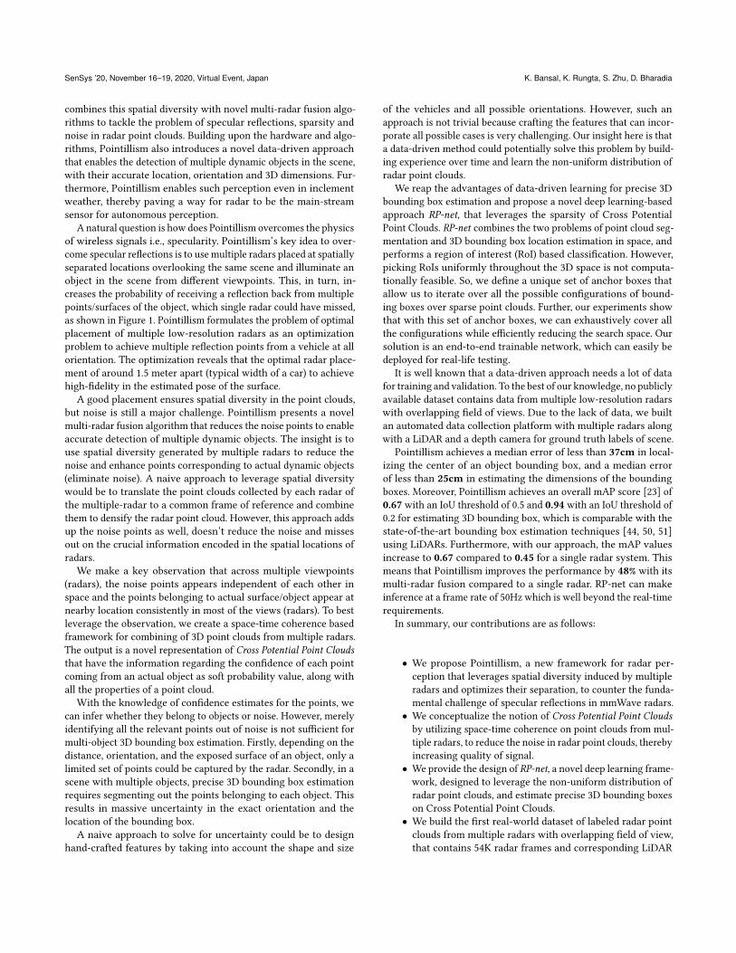
Single 0.5m 1m 2m 3mGT orientation
Figure 4: Wireless Insite simulations: Point clouds with single radaror smaller separation could lead to ambiguity in pose of the car whichgets eliminated by increasing radar separation. Orange and blue pointsare from 2 different radars.
Figure 5: Comparison of average error in radian between single andmultiple radars. For a separation greater than 1.5m, the performanceimproves.
the car at several locations in an area of 10m×10m in front of the
radar(s). At each location, simulations are created for multiple ori-
entations(angles) of car, spanning 360 degrees in 36 discrete steps.
For each placement and orientation, we consider two radar setups:
Single radar and Two radars with varying separation distance. In sim-
ulations, the radars can resolve all the rays returning to the receiver
(perfect resolution). With this, we can independently compare how
the geometry of the scene affects performance.
3.2 Performance comparison of single andmultiple radars
For a rectangular bounding box of a car, the system that captures
more surface points (less affected by specularity) would perform
better in estimating the bounding box’s orientation. To estimate
the orientation angle of the box from point clouds, we use an MLP
(multi-layer perceptron) regressor from scikit-learn [41] trained on
the data generated from the simulations. MLP regressor takes a
simulated point cloud as input and outputs the orientation angle of
the car. Figure 5 shows the comparison of performance in terms of
the mean error made in angle estimation. We make two important
observations from these results. Firstly, the results show that the
two radar system outperforms the single radar system. Secondly,
a more interesting observation is that there is a sharp increase in
performance between the separations 1.5m and 2m. It remains rela-
tively constant before and after. The width of the car we used in
simulations is ≈ 1.7m, which is the width of a standard car. Hence,
the results show that the optimal distance between two radars for
estimating a bounding box on a vehicle should be comparable to
the vehicle’s width. Figure 4 further shows how increasing the sep-
aration between radars would improve the point cloud generated.
3
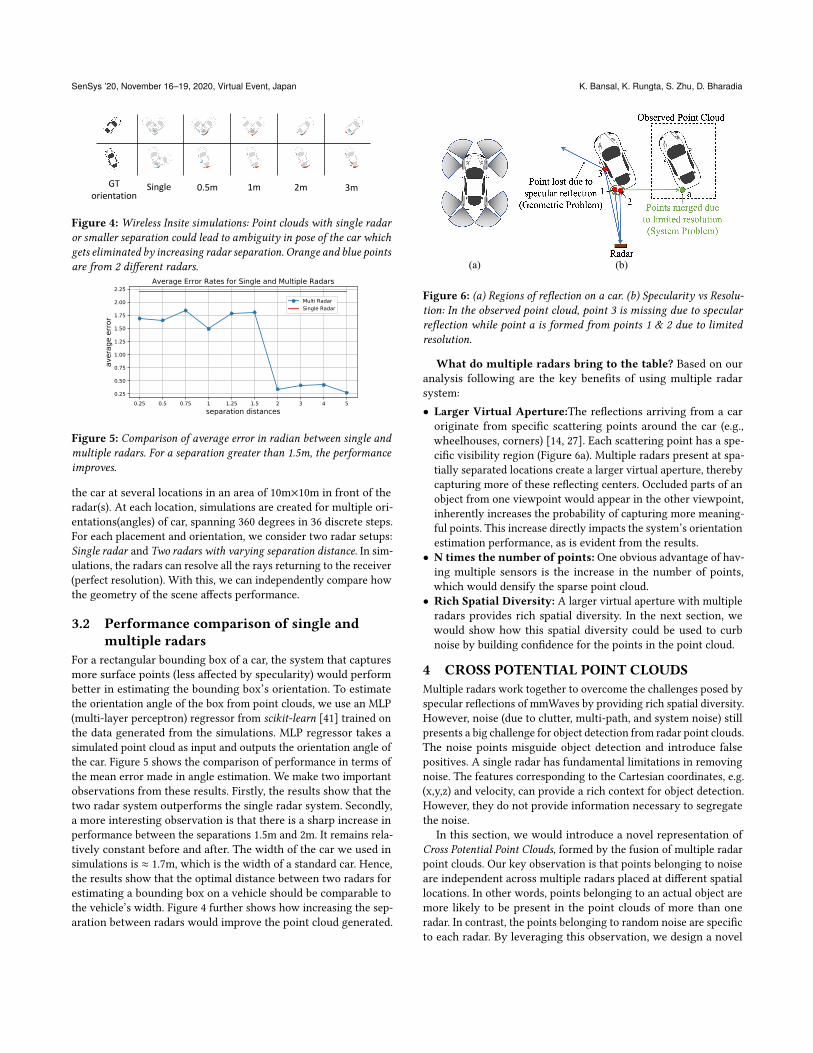
12
aPoint lost due to
specular reflection(Geometric Problem) Points merged due
to limited resolution(System Problem)
Radar
Observed Point Cloud(a) (b)
Figure 6: (a) Regions of reflection on a car. (b) Specularity vs Resolu-tion: In the observed point cloud, point 3 is missing due to specularreflection while point a is formed from points 1 & 2 due to limitedresolution.
What do multiple radars bring to the table? Based on our
analysis following are the key benefits of using multiple radar
system:
• Larger Virtual Aperture:The reflections arriving from a car
originate from specific scattering points around the car (e.g.,
wheelhouses, corners) [14, 27]. Each scattering point has a spe-
cific visibility region (Figure 6a). Multiple radars present at spa-
tially separated locations create a larger virtual aperture, thereby
capturing more of these reflecting centers. Occluded parts of an
object from one viewpoint would appear in the other viewpoint,
inherently increases the probability of capturing more meaning-
ful points. This increase directly impacts the system’s orientation
estimation performance, as is evident from the results.
• N times the number of points: One obvious advantage of hav-ing multiple sensors is the increase in the number of points,
which would densify the sparse point cloud.
• Rich Spatial Diversity: A larger virtual aperture with multiple
radars provides rich spatial diversity. In the next section, we
would show how this spatial diversity could be used to curb
noise by building confidence for the points in the point cloud.
4 CROSS POTENTIAL POINT CLOUDSMultiple radars work together to overcome the challenges posed by
specular reflections of mmWaves by providing rich spatial diversity.
However, noise (due to clutter, multi-path, and system noise) still
presents a big challenge for object detection from radar point clouds.
The noise points misguide object detection and introduce false
positives. A single radar has fundamental limitations in removing
noise. The features corresponding to the Cartesian coordinates, e.g.
(x,y,z) and velocity, can provide a rich context for object detection.
However, they do not provide information necessary to segregate
the noise.
In this section, we would introduce a novel representation of
Cross Potential Point Clouds, formed by the fusion of multiple radar
point clouds. Our key observation is that points belonging to noise
are independent across multiple radars placed at different spatial
locations. In other words, points belonging to an actual object are
more likely to be present in the point clouds of more than one
radar. In contrast, the points belonging to random noise are specific
to each radar. By leveraging this observation, we design a novel
Pointillism: Accurate 3D Bounding Box Estimation with Multi-Radars SenSys ’20, November 16–19, 2020, Virtual Event, Japan
Target Vehicle
Multiple Radars on Source Vehicle
Large separation between Ghost
Cluster Centroids
Small separation between Target Cluster centroids
Figure 7: Formation of ghost clusters due to multipath. The centroidsin the ghost clusters are more separated in comparison to the centroidof target cluster and given low potential values in Cross PotentialPoint Clouds.
algorithm that filters noise from radar point clouds and creates low-
noise Cross Potential Point Clouds. In the following subsection, we
would describe how we can use the data from multiple radars to
encode information regarding noise.
4.1 Space coherence with Radar point potentialNoise harms the bounding box estimation as it creates false posi-
tives. Our key insight on tackling noise takes inspiration from sig-
nal processing techniques. In signal processing, we collect multiple
noisy data stream and take their average to reduce the noise vari-
ance and improve the overall SNR (signal to noise ratio). The idea is
that the signal present in each data stream adds up coherently. At
the same time, the noise is random and will not add constructively.
While the idea is intuitive, it is non-trivial to extend it to the point
clouds. We cannot simply add point clouds from multiple radars
in the hope to reduce noise because of the following reasons: (1)
The 3D point cloud is sparse and incoherent in space, i.e., multiple
radars may capture different points in 3D space for the same target
object. (2) It is hard to build confidence for every point, whether it
contributes to the object bounding box or corresponds to the noise
point (generated by clutter or multi-path).
To apply the space coherence in the point cloud domain, we use
the geometric information of point clouds. The above insight prop-
agates to the fact that if a region of 3D space generates a response
in multiple radars, it is likely to be generated from an object and
not noise. To capture this effect, we need to measure the coherence
between point clouds originating from multiple radars across 3D
space. As shown in Figure 6, radar points from an object are clus-
tered around some scattering regions on a vehicle. By identifying
these clusters, we can define our confidence of a point being gen-
erated from an object by looking at the same scattering region in
multiple radar point clouds (space coherence). Our approach runs
in two steps: (a) Clustering the point clouds and (b) Enforcing space
coherence by defining cross-potentials, detailed as follows:
(a) Clustering the point clouds: Radar point clouds are presentin the form of clusters of points originating from a scattering re-
gion on the object (Section 3). We use the standard DBSCAN [20]
algorithm to find clusters in our point cloud. DBSCAN works on
the notion of defining a neighborhood of points based on distance 𝜖
given as an input parameter. If a specific number of points (another
input parameter) is present in that neighborhood, the point and
its neighborhood are identified as a cluster. For each cluster 𝑖 , the
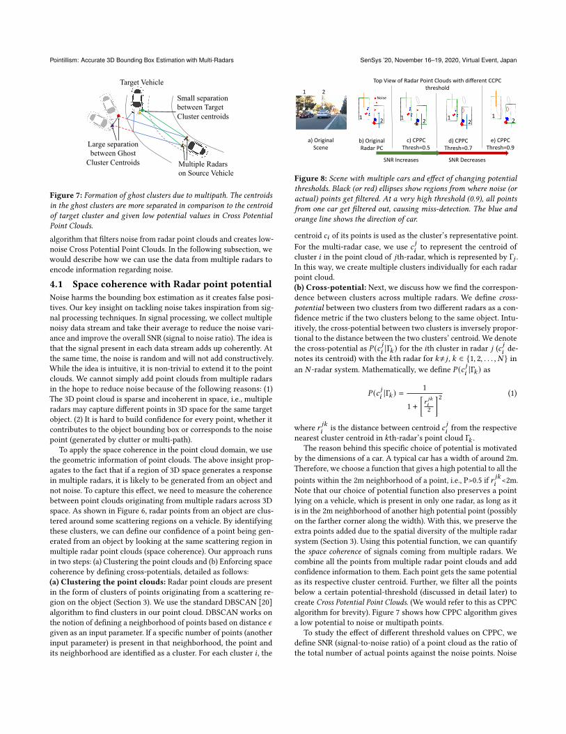
b) Original Radar PC
c) CPPC Thresh=0.5
e) CPPC Thresh=0.9
d) CPPC Thresh=0.7
SNR Increases SNR Decreases
a) Original Scene
Top View of Radar Point Clouds with different CCPC threshold
Noise21
1 1 1 12 2 2 2
Figure 8: Scene with multiple cars and effect of changing potentialthresholds. Black (or red) ellipses show regions from where noise (oractual) points get filtered. At a very high threshold (0.9), all pointsfrom one car get filtered out, causing miss-detection. The blue andorange line shows the direction of car.
centroid 𝑐𝑖 of its points is used as the cluster’s representative point.
For the multi-radar case, we use 𝑐𝑗𝑖to represent the centroid of
cluster 𝑖 in the point cloud of 𝑗th-radar, which is represented by Γ𝑗 .In this way, we create multiple clusters individually for each radar
point cloud.
(b) Cross-potential: Next, we discuss how we find the correspon-
dence between clusters across multiple radars. We define cross-potential between two clusters from two different radars as a con-
fidence metric if the two clusters belong to the same object. Intu-
itively, the cross-potential between two clusters is inversely propor-
tional to the distance between the two clusters’ centroid. We denote
the cross-potential as 𝑃 (𝑐 𝑗𝑖|Γ𝑘 ) for the 𝑖th cluster in radar 𝑗 (𝑐
𝑗𝑖de-
notes its centroid) with the 𝑘th radar for 𝑘≠ 𝑗 , 𝑘 ∈ {1, 2, . . . , 𝑁 } inan 𝑁 -radar system. Mathematically, we define 𝑃 (𝑐 𝑗
𝑖|Γ𝑘 ) as
𝑃 (𝑐 𝑗𝑖|Γ𝑘 ) =
1
1 +[𝑟𝑗𝑘
𝑖
2
]2
(1)
where 𝑟𝑗𝑘𝑖
is the distance between centroid 𝑐𝑗𝑖from the respective
nearest cluster centroid in 𝑘th-radar’s point cloud Γ𝑘 .The reason behind this specific choice of potential is motivated
by the dimensions of a car. A typical car has a width of around 2m.
Therefore, we choose a function that gives a high potential to all the
points within the 2m neighborhood of a point, i.e., P>0.5 if 𝑟𝑗𝑘𝑖<2m.
Note that our choice of potential function also preserves a point
lying on a vehicle, which is present in only one radar, as long as it
is in the 2m neighborhood of another high potential point (possibly
on the farther corner along the width). With this, we preserve the
extra points added due to the spatial diversity of the multiple radar
system (Section 3). Using this potential function, we can quantify
the space coherence of signals coming from multiple radars. We
combine all the points from multiple radar point clouds and add
confidence information to them. Each point gets the same potential
as its respective cluster centroid. Further, we filter all the points
below a certain potential-threshold (discussed in detail later) to
create Cross Potential Point Clouds. (We would refer to this as CPPC
algorithm for brevity). Figure 7 shows how CPPC algorithm gives
a low potential to noise or multipath points.
To study the effect of different threshold values on CPPC, we
define SNR (signal-to-noise ratio) of a point cloud as the ratio of
the total number of actual points against the noise points. Noise
SenSys ’20, November 16–19, 2020, Virtual Event, Japan K. Bansal, K. Rungta, S. Zhu, D. Bharadia
Low to Heavy Noise Reduction
No or very low noise cases
Decrease in SNR for higher thresh:
For <=0.5
For <=0.7
For <=0.9
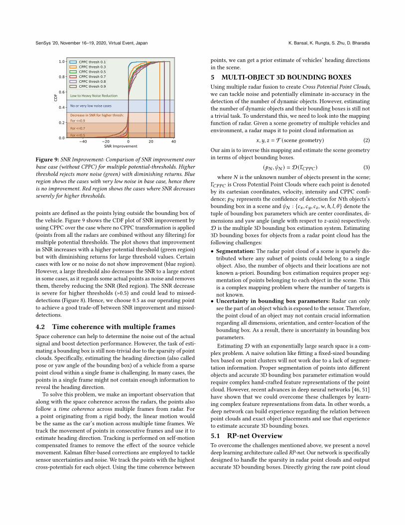
Figure 9: SNR Improvement: Comparison of SNR improvement overbase case (without CPPC) for multiple potential-thresholds. Higherthreshold rejects more noise (green) with diminishing returns. Blueregion shows the cases with very low noise in base case, hence thereis no improvement. Red region shows the cases where SNR decreasesseverely for higher thresholds.
points are defined as the points lying outside the bounding box of
the vehicle. Figure 9 shows the CDF plot of SNR improvement by
using CPPC over the case where no CPPC transformation is applied
(points from all the radars are combined without any filtering) for
multiple potential thresholds. The plot shows that improvement
in SNR increases with a higher potential threshold (green region)
but with diminishing returns for large threshold values. Certain
cases with low or no noise do not show improvement (blue region).
However, a large threshold also decreases the SNR to a large extent
in some cases, as it regards some actual points as noise and removes
them, thereby reducing the SNR (Red region). The SNR decrease
is severe for higher thresholds (>0.5) and could lead to missed-
detections (Figure 8). Hence, we choose 0.5 as our operating point
to achieve a good trade-off between SNR improvement and missed-
detections.
4.2 Time coherence with multiple framesSpace coherence can help to determine the noise out of the actual
signal and boost detection performance. However, the task of esti-
mating a bounding box is still non-trivial due to the sparsity of point
clouds. Specifically, estimating the heading direction (also called
pose or yaw angle of the bounding box) of a vehicle from a sparse
point cloud within a single frame is challenging. In many cases, the
points in a single frame might not contain enough information to
reveal the heading direction.
To solve this problem, we make an important observation that
along with the space coherence across the radars, the points also
follow a time coherence across multiple frames from radar. For
a point originating from a rigid body, the linear motion would
be the same as the car’s motion across multiple time frames. We
track the movement of points in consecutive frames and use it to
estimate heading direction. Tracking is performed on self-motion
compensated frames to remove the effect of the source vehicle
movement. Kalman filter-based corrections are employed to tackle
sensor uncertainties and noise. We track the points with the highest
cross-potentials for each object. Using the time coherence between
points, we can get a prior estimate of vehicles’ heading directions
in the scene.
5 MULTI-OBJECT 3D BOUNDING BOXESUsing multiple radar fusion to create Cross Potential Point Clouds,we can tackle noise and potentially eliminate in-accuracy in the
detection of the number of dynamic objects. However, estimating
the number of dynamic objects and their bounding boxes is still not
a trivial task. To understand this, we need to look into the mapping
function of radar. Given a scene geometry of multiple vehicles and
environment, a radar maps it to point cloud information as
𝑥,𝑦, 𝑧 = F (scene geometry) (2)
Our aim is to inverse this mapping and estimate the scene geometry
in terms of object bounding boxes.
(𝑝𝑁 ,𝜓𝑁 ) = D(Γ𝐶𝑃𝑃𝐶 ) (3)
where 𝑁 is the unknown number of objects present in the scene;
Γ𝐶𝑃𝑃𝐶 is Cross Potential Point Clouds where each point is denoted
by its cartesian coordinates, velocity, intensity and CPPC confi-
dence; 𝑝𝑁 represents the confidence of detection for 𝑁 th objects’s
bounding box in a scene and𝜓𝑁 : {𝑐𝑥 , 𝑐𝑦, 𝑐𝑧 ,𝑤, ℎ, 𝑙, \ } denote thetuple of bounding box parameters which are center coordinates, di-
mensions and yaw angle (angle with respect to 𝑧-axis) respectively.
D is the multiple 3D bounding box estimation system. Estimating
3D bounding boxes for objects from a radar point cloud has the
following challenges:
• Segmentation: The radar point cloud of a scene is sparsely dis-
tributed where any subset of points could belong to a single
object. Also, the number of objects and their locations are not
known a-priori. Bounding box estimation requires proper seg-
mentation of points belonging to each object in the scene. This
is a complex mapping problem where the number of targets is
not known.
• Uncertainty in bounding box parameters: Radar can only
see the part of an object which is exposed to the sensor. Therefore,
the point cloud of an object may not contain crucial information
regarding all dimensions, orientation, and center-location of the
bounding box. As a result, there is uncertainty in bounding box
parameters.
Estimating D with an exponentially large search space is a com-
plex problem. A naive solution like fitting a fixed-sized bounding
box based on point clusters will not work due to a lack of segmen-
tation information. Proper segmentation of points into different
objects and accurate 3D bounding box parameter estimation would
require complex hand-crafted feature representations of the point
cloud. However, recent advances in deep neural networks [46, 51]
have shown that we could overcome these challenges by learn-
ing complex feature representations from data. In other words, a
deep network can build experience regarding the relation between
point clouds and exact object placements and use that experience
to estimate accurate 3D bounding boxes.
5.1 RP-net OverviewTo overcome the challenges mentioned above, we present a novel
deep learning architecture called RP-net. Our network is specificallydesigned to handle the sparsity in radar point clouds and output
accurate 3D bounding boxes. Directly giving the raw point cloud

Pointillism: Accurate 3D Bounding Box Estimation with Multi-Radars SenSys ’20, November 16–19, 2020, Virtual Event, Japan
Nx2
56
Anchor Box Proposal
Max
mlp 1 x 1024K x 259
Box Refinement Parameters
NMS1 x 1024
b) Feature pooling
mlpAnchor Box Confidence
Scores
Selected Box Features
M boxes Pooled features
(shared)
Fully Connected
Fully Connected
(64,128,256)(512,1024)
Representative features for M boxes
(512,256,2)
(512,256,7)
a) Region Proposal
c) Confidence
d) Refinement
Anchor Point
Input Point Cloud
Output 3D Boxes
Figure 10: RP-net architecture: a) Our network takes CPPC as input with N points and 6 channels, extracts features using a pointnet layer,and generates anchor boxes for each point. b) A Feature pooling layer pools point features from K points lying inside each box, which are passedthrough pointnet and max pool layers to generate representative features for anchors. c) Confidence values are predicted for each anchor. d) Highconfidence anchors are taken to the box refinement stage. The output is a set of 3D bounding boxes for each object in the scene (top view box isshown).as an input can not solve the problem due to the unknown number
and locations of the objects in the scene. Usually, an object detector
uses a fixed set of initial region proposals to solve this problem.
Our network proposes a novel way of generating these region
proposals (anchor boxes), based on the radar response due to vehicle
geometry and space-time coherence. Unlike LiDAR, where many
points originate from ground and other static objects like buildings,
radar data is sparse and contains mostly the points from dynamic
and metallic objects like cars after CPPC noise suppression due to
strong EM reflective properties of metals. Specifically, the sparsity
in radar data and the fact that all the points originate from the
vehicles’ surface allow us to define point-based region proposals.
These fixed size anchor boxes are used as initial estimates of 3D
bounding boxes. The size of these anchor boxes is determined by
the average size of vehicles in the training dataset. Now, instead of
the entire scene point cloud, the network works separately on each
of these anchor boxes. For each of these anchor boxes, the task is
reduced to generate a confidence number 𝑝 of whether the points
inside that anchor box belongs to an object.
Confidence scores are generated for all the anchor boxes. A set
of high confidence boxes is chosen. These anchor boxes are passed
through a refinement stage that solves the uncertainty issue in
bounding box parameters. In this stage, the anchor boxes are refined
to provide accurate 3D bounding boxes of the objects present in
the scene (parameter𝜓 ).
5.2 Network Architecture DesignThe job of RP-net is that given a scene point cloud, output the
set of 3D bounding boxes of the objects present in the scene. It
takes CPPC as input, which has 6 channels corresponding to x,y,z
coordinates, velocity, peak intensities, and cross-potential values
for each point. RP-net comprises of following blocks:
(a) Handling Multiple Objects.For a given scene with multiple
vehicles, region proposals are defined by placing multiple anchor
boxes in the scene. As mentioned above, we propose a novel point-
based region proposal (anchor boxes) generation scheme based
on the radar response due to vehicle geometry and space-time
coherence. Given a point, we use five different placements of anchor
box around the point (we call this point as anchor point for those
anchor boxes. Refer Figure 10). We use the pose values derived for
each anchor point using space-time coherence for the orientation
angle, as explained in Section 4.
(b) Segmentation by Feature Extraction and pooling. Our ob-jective is to perform classification and 3D bounding box parameter
regression by learning meaningful feature representations from
the point cloud data. RP-net extracts these features in two stages,
i.e., before and after generating anchor boxes. We first use a point-
net [46] encoder of shared MLP to extract features from the entire
point cloud. We would refer the reader to [46] for an in-depth
understanding of pointnets.
In the second stage, the anchor boxes are determined for each
point. An RoI (Region of Interest) feature pooling block of the
network pools the features from all the points lying inside an anchor
box. These features are passed through another pointnet layer and
then max pooled into a single representative feature for every
anchor box defined per scene.
(c) Bounding Box confidence prediction. The entire set of rep-resentative features of anchor boxes, obtained after the previous
block, is passed through a classification network consisting of fully
connected layers. The fully connected layers learn a mapping from
anchor boxes’ representative features to the confidence value for
each box.
Performing classification on RoI based max-pooled features al-
ways ensures that the contextual information from all neighborhood
points of the anchor point, lying inside the anchor box is accounted,
leading to better classification results. The problem of segmentation
is solved by performing classification directly on the anchor boxes.
The network will learn to choose the corresponding anchor box
with high confidence, which contains all the points belonging to
an object.
(d) Refinement of Box Parameters. In the previous step, the an-
chor boxes were rough estimates of the dimensions, center, and
orientation of final 3D bounding boxes as we used fixed-size anchor
boxes. We still need further refinement of these parameters to get
accurate bounding boxes. Note that this step is quite essential to es-
timate the accurate dimensions and location of the boxes. After the
classification step, we obtain the confidence scores for all the anchor

SenSys ’20, November 16–19, 2020, Virtual Event, Japan K. Bansal, K. Rungta, S. Zhu, D. Bharadia
boxes. Since we obtained anchor boxes for each point, there could
be many overlapping high confidence boxes belonging to the same
object. Non-maximal suppression(NMS) sampling is performed on
this set using the confidence values. NMS sampling removes boxes
which have a high overlap with another high confidence box of
the same object. The representative features from the remaining
anchor boxes are passed through three fully connected layers to
output a tuple [ℎ′,𝑤 ′, 𝑙 ′, 𝑥 ′, 𝑦′, 𝑧′, \ ′] corresponding to refinements
of length, breadth, height, center coordinates, and orientation an-
gle respectively. These refinements are added to the anchor box
parameters to generate the final 3D bounding box prediction.
(e) Loss functions. The anchor box classification in the first stage
of the network is a binary classification problem that uses a cross-
entropy loss, given by
L𝑅𝑃𝑁 =
𝑁∑︁𝑖=1
−(𝑦𝑖 log(𝑝𝑖 ) + (1 − 𝑦𝑖 ) log(1 − 𝑝𝑖 )) (4)
where 𝑦𝑖 = [0, 1] is the ground truth and 𝑝𝑖 is the predicted con-
fidence value. Refinement of the bounding boxes is a regression
problem and we use Smooth-L1 loss for this purpose. The loss is
given by:
L𝑟𝑒 𝑓 𝑖𝑛𝑒𝑚𝑒𝑛𝑡 (𝑟, 𝑟 ′) ={1
2(𝑟 − 𝑟 ′)2, for |𝑟 − 𝑟 ′ | < 1.
𝛿 |𝑟 − 𝑟 ′ | − 1
2, otherwise.
(5)
where 𝑟 and 𝑟 ′ are ground truth and regressed refinement values
respectively for each parameter [ℎ′,𝑤 ′, 𝑙 ′, 𝑥 ′, 𝑦′, 𝑧′, \ ′].
6 EXPERIMENTAL SETUP AND DATASET
Parameter Value Parameter ValueStart Frequency 77 GHz Frame rate 30 fps
Bandwidth 2240 MHz Range Res. 0.067m
ADC rate 7500 ksps Velocity Res. 2.59 m/s
Chirp Duration 40 `s Max velocity 20.74 m/s
Table 1: Values of the radar parameters used. (Res.=resolution)The use of radars for perception in autonomous systems is quite
recent. No publicly available dataset collects data from multiple
radar sensors with overlapping fields of view in 3D. We collect our
own dataset for training and testing Pointillism. We collected data
from three sensors: a 16 channel Ouster LiDAR [4] placed and an
Intel RealSense D415 [2] Camera at the center of a rail , and 2 TI
IWR1443BOOST [1] radars placed at the end-points of the rail at
a distance of 1.5m, all placed on a car. Figure 12 shows our data
collection platform. We use LiDAR for ground truth annotations
and camera for visualization only. Data is labeled using an online
tool called scalabel [7]. All the sensors are controlled using a centralcontroller running ROS (Robotic Operating System), running on
a laptop placed in the car. Each data frame is timestamped for
synchronizing the sensors. We perform controlled experimentation
based sensor calibration. The data from all the sensors are brought
to the same coordinate system by deriving extrinsic matrices for
each sensor. Our hardware design is modular so that sensors can
be swapped, and only data extraction for that sensor needs to be
updated.
Each radar has a 3Tx and 4Rx MIMO antenna array. We use the
FMCW processing chain provided by TI for generating point clouds
Figure 11: Dataset Distribution: Histogram plots of the dimensionsof the vehicles present in the dataset. It includes small golf carts tolarge buses.
Tx/Rx
Figure 12: Pointillism data collection platform. (Top Left) 16-channel Ouster LiDAR, RealSense Depth Camera for ground truthlabels. (Top Right) our radars. (Bottom) Our System: Two radars,LiDAR, Depth camera combined synchronously to common clock.
characterized by x,y,z coordinates, doppler, and the intensity (peak
values) of points [1]. Table 1 summarizes the operating parameters
of our radars. Figure 11 shows the distribution of the different sizes
of objects/cars present in our dataset. The dataset includes small
golf carts to large buses with a maximum number of 4 objects in the
scene. In total, we collect 54K radar frames for five real-life traffic
and driving scenes. Data was collected in different operating condi-
tions, including day, night, and adverse weather (fog) conditions
(smoke machine experiments). It is the first of its kind radar dataset
with data from multiple radars, LiDARs, and RGB cameras that can
enable various sensor-fusion-based approaches. We will release the
dataset for public use. We plan to keep expanding this dataset with
more samples over time.
7 IMPLEMENTATIONIn this section we would describe the implementation details of
Pointillism.
Deep learning parameters: For implementing our network, we
use the PyTorch framework. The number of output channels is men-
tioned above each layer in Figure 10. We use Adam optimizer with
a learning rate of 0.0002 and momentum 0.9. A batch-normalization
layer follows each layer of the network. We use (2m, 2m, 5m) as
(width, height, length) to initialize the anchor boxes’ dimensions. 70
random points are sampled from each Cross Potential Point Clouds

Pointillism: Accurate 3D Bounding Box Estimation with Multi-Radars SenSys ’20, November 16–19, 2020, Virtual Event, Japan
Figure 13: Predicted 3D bounding boxes using only radar (red) alongwith ground truth boxes (blue). The 3D IoUs of predictions are 0.52,0.43 & 0.83 respectively. Radars can be used as a standalone sensorfor object detection despite sparsity and low resolution.
for giving input to the network. The network takes 6 channel inputs
for xyz-coordinates, velocity, peak intensity values, and confidence
estimates. We sample 32 points at random from all the points lying
inside an anchor box during the feature pooling stage. If the num-
ber of points is less than 32, then the same points are repeated to
maintain consistency throughout network operation.
End-to-end training and deployment: For training the classifi-cation network, ground truth is generated based on the IoU (Inter-
section over Union) values of the anchor boxes against the ground
truth bounding boxes. We use the top view of the anchor boxes to
calculate 2D IoUs. We choose choose top 100 anchor boxes based on
IoU match for classification. Boxes with 2D IoU overlap of greater
than 0.2 are considered as positive examples for classification. For
the refinement network, NMS is performed on the boxes to remove
boxes with more than 0.5 2D IoU overlap using predicted confi-
dence scores. The training happens simultaneously for both region
proposal and the refinement network. However, at the start of the
training, the classification head can not provide correct confidence
scores; hence, for the initial 30 epochs, we use 2D IoU scores with
ground-truth boxes as confidence values for NMS. Note that the
network is already trained during the testing phase, and we do not
need these IoU values.
8 EVALUATIONIn this section, we would comprehensively evaluate each part of
Pointillism. We would compare our results against the commonly
used deterministic clustering [59] and deep learning based ap-
proaches [51] for 3D bounding box estimation on point clouds.
Figure 13 shows examples of predicted 3D bounding boxes by
Pointillism.
Testing and Training data-set: We test our system on the
dataset collected by us (section 6) that contains 54000 radar frames.
We use a train test split of 9:1. The data used for testing comes
from separate data collection runs than training data to ensure the
generalization of our approach. We also use the publicly available
astyx dataset [39] for automotive radars to demonstrate the gen-
eralization of our approach. We also compare the performance of
Pointillism against LiDAR in bad weather conditions.
Following are the metrics we use to evaluate our system:
• IoU: IoU (Jaccard Index) is a measure of the overlap between the
predicted bounding box and the ground truth box. 3D IoU is given
byIntersection Volume
Union Volume. 2D IoU is defined for the top view (also
called Bird-eye-view (BEV)) rectangles of 3D bounding boxes, as
Intersection Area
Union Area. Two equal-sized boxes with half overlap would
have an IoU of 0.33. Hence, even an IoU of around 0.5 is generally
regarded as a good overlap.
• mAP: (mean Average Precision) mAP is the area under the
precision-recall (PR) curve, which is a measure of the number of
actual boxes detected (recall) along with the accuracy of detec-
tions (precision). Specifically, precision is obtained for incremen-
tal recall values to get PR curve.
𝑃𝑟𝑒𝑐𝑖𝑠𝑖𝑜𝑛 = 𝑇𝑃/(𝑇𝑃 + 𝐹𝑃)𝑅𝑒𝑐𝑎𝑙𝑙 = 𝑇𝑃/(𝑇𝑃 + 𝐹𝑁 )𝑚𝐴𝑃 = 𝐴𝑟𝑒𝑎(precision-recall curve)
An estimation is regarded as a true positive (TP) if it is above
a particular IoU (Intersection Over Union) threshold. Note that
a higher recall rate can easily be obtained by predicting a large
number of boxes, but at the cost of sacrificing precision (more
False Positives (FP)) and vice-versa. A higher mAP means better
performance on both accuracy (precision) and exhaustiveness
(recall) of estimation. An FP could also be obtained because of
noise. An FP generated due to noise will have a very small (almost
0) IoU with any ground truth box. Hence, in a lower IoU threshold
regime, the mAP is more sensitive to the amount of noise and
allows us to better compare our noise suppression performance.
In summary, Pointillism achieves a median error of less than
37cm in localizing the center of an object bounding box and a
median error of less than 25cm in estimating the dimensions of the
bounding boxes. We use 2D IoU (BEV IoU) as the thresholds for our
mAP metric [23]. Pointillism achieves an mAP score of 0.67 for an
IoU threshold of 0.5 and a score of 0.94 for a lower IoU threshold
of 0.2, which is a 45% improvement over a single radar system. We
further show that RP-net is easily generalizable to other datasets
by evaluating its performance on Astyx dataset [39] and achieve
an mAP of 0.65 with IoU threshold of 0.2.
8.1 Performance on Bounding Box estimationOur entire system (dubbed RP-MR-CPPC) consists of multi-radar
(MR) fusion to create Cross Potential Point Clouds (CPPC) and
RP-net to estimate 3D bounding box. To individually compare the
mAP performance of CPPC and RP-net we define the following
baselines:
• RP-SR: RP-net on single radar data.
• RP-MR: RP-net on multiple radar data without Cross Potential
Point Clouds fusion. The point clouds from multiple radars are
simply added in the global coordinate system.
• Clust: A clustering based bounding box estimation baseline. A
predefined size bounding box is estimated for each cluster found
using DBSCAN, coupled with angle estimation using PrincipleComponent Analysis [56]
• Clust-CPPC: The clustering based approach used on Cross Po-
tential Point Clouds.
• PointRCNN: Official implementation of well-known LiDAR
based 3D bounding box estimation network PointRCNN [51]
used on our collected dataset.
Figure 14a shows the overall performance of these systems. The
X-axis is the IoU thresholds used for the mAP values. Further, to
best examine the performance improvement brought in by CPPC,
we also evaluate the performance on a subset of validation set that
contains hard examples following KiTTi evaluation framework [23].
Hard examples are characterized by point clouds containing more
than one-fourth of the points coming from noise, and the cars are
SenSys ’20, November 16–19, 2020, Virtual Event, Japan K. Bansal, K. Rungta, S. Zhu, D. Bharadia
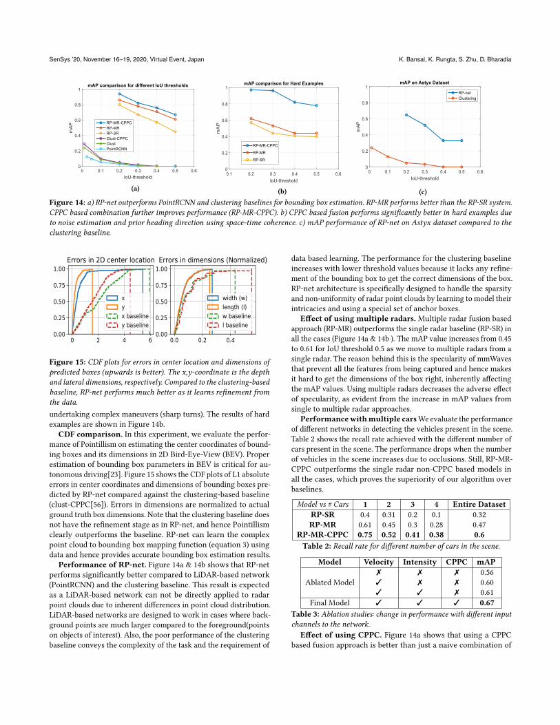
(a) (b) (c)Figure 14: a) RP-net outperforms PointRCNN and clustering baselines for bounding box estimation. RP-MR performs better than the RP-SR system.CPPC based combination further improves performance (RP-MR-CPPC). b) CPPC based fusion performs significantly better in hard examples dueto noise estimation and prior heading direction using space-time coherence. c) mAP performance of RP-net on Astyx dataset compared to theclustering baseline.
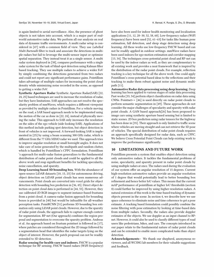
Figure 15: CDF plots for errors in center location and dimensions ofpredicted boxes (upwards is better). The x,y-coordinate is the depthand lateral dimensions, respectively. Compared to the clustering-basedbaseline, RP-net performs much better as it learns refinement fromthe data.undertaking complex maneuvers (sharp turns). The results of hard
examples are shown in Figure 14b.
CDF comparison. In this experiment, we evaluate the perfor-
mance of Pointillism on estimating the center coordinates of bound-
ing boxes and its dimensions in 2D Bird-Eye-View (BEV). Proper
estimation of bounding box parameters in BEV is critical for au-
tonomous driving[23]. Figure 15 shows the CDF plots of L1 absolute
errors in center coordinates and dimensions of bounding boxes pre-
dicted by RP-net compared against the clustering-based baseline
(clust-CPPC[56]). Errors in dimensions are normalized to actual
ground truth box dimensions. Note that the clustering baseline does
not have the refinement stage as in RP-net, and hence Pointillism
clearly outperforms the baseline. RP-net can learn the complex
point cloud to bounding box mapping function (equation 3) using
data and hence provides accurate bounding box estimation results.
Performance of RP-net. Figure 14a & 14b shows that RP-net
performs significantly better compared to LiDAR-based network
(PointRCNN) and the clustering baseline. This result is expected
as a LiDAR-based network can not be directly applied to radar
point clouds due to inherent differences in point cloud distribution.
LiDAR-based networks are designed to work in cases where back-
ground points are much larger compared to the foreground(points
on objects of interest). Also, the poor performance of the clustering
baseline conveys the complexity of the task and the requirement of
data based learning. The performance for the clustering baseline
increases with lower threshold values because it lacks any refine-
ment of the bounding box to get the correct dimensions of the box.
RP-net architecture is specifically designed to handle the sparsity
and non-uniformity of radar point clouds by learning to model their
intricacies and using a special set of anchor boxes.
Effect of using multiple radars.Multiple radar fusion based
approach (RP-MR) outperforms the single radar baseline (RP-SR) in
all the cases (Figure 14a & 14b ). The mAP value increases from 0.45
to 0.61 for IoU threshold 0.5 as we move to multiple radars from a
single radar. The reason behind this is the specularity of mmWaves
that prevent all the features from being captured and hence makes
it hard to get the dimensions of the box right, inherently affecting
the mAP values. Using multiple radars decreases the adverse effect
of specularity, as evident from the increase in mAP values from
single to multiple radar approaches.
Performancewithmultiple carsWeevaluate the performance
of different networks in detecting the vehicles present in the scene.
Table 2 shows the recall rate achieved with the different number of
cars present in the scene. The performance drops when the number
of vehicles in the scene increases due to occlusions. Still, RP-MR-
CPPC outperforms the single radar non-CPPC based models in
all the cases, which proves the superiority of our algorithm over
baselines.
Model vs # Cars 1 2 3 4 Entire DatasetRP-SR 0.4 0.31 0.2 0.1 0.32
RP-MR 0.61 0.45 0.3 0.28 0.47
RP-MR-CPPC 0.75 0.52 0.41 0.38 0.6Table 2: Recall rate for different number of cars in the scene.
Model Velocity Intensity CPPC mAP
Ablated Model
✗ ✗ ✗ 0.56
✓ ✗ ✗ 0.60
✓ ✓ ✗ 0.61
Final Model ✓ ✓ ✓ 0.67Table 3: Ablation studies: change in performance with different inputchannels to the network.
Effect of using CPPC. Figure 14a shows that using a CPPC
based fusion approach is better than just a naive combination of

Pointillism: Accurate 3D Bounding Box Estimation with Multi-Radars SenSys ’20, November 16–19, 2020, Virtual Event, Japan
multiple radar point clouds (RP-MR). In the hard examples (fig-
ure 14b) the effect is even more significant. The performance in-
creases from 0.44 to 0.78 by using CPPC on multiple radars for IoU
threshold of 0.5. Note that even for the clustering based baseline,
using CPPC fusion improves the results for bounding box estima-
tion. The space-time coherence in CPPC reduces the noise, thereby
minimizing false positives and improving results.
Comparison to other approaches (LiDAR/sensor fusion).In order to put these results into perspective, we provide some
results from LiDAR-based approaches. PointRCNN [51] achieves
0.78 mAP on KiTTi LiDAR dataset [23]. A camera and radar fusion
approach, on a dataset provided by Astyx GMBH [39], achieves an
mAP value of 0.45 on the complete dataset. Although it is not fair to
directly compare with the LiDAR results, as the underlying datasets
and IoU thresholds used are different (LiDAR-based approaches use
a higher IoU threshold of 0.7), but we want to emphasise on the
fact that it is possible to achieve LiDAR or camera like perception
using just radars. Moreover, a higher resolution radar can produce a
denser point cloud, that would further increase the IoU performance
using our method.
Model mAP (IoU>0.5) Time256 channels 0.50 0.018 seconds (55 fps)
1024 channels 0.68 0.0208 seconds (48 fps)
Table 4: Effect of model size on time and performance
8.2 Model Generalization on Astyx datasetIn order to evaluate the generalization of our network, we test our
network on the recently released Astyx dataset [39]. The released
data set contains only 545 scene point clouds, which are quite less
in order to allow efficient training. Also, the dataset contains only a
single radar, which prevents us from applying our entire processing
chain to the dataset. We divide the dataset into 5% test (and rest
training) set and evaluate the object detection performance. RP-net
is able to achieve a performance of 0.65 mAP on this dataset with
an IoU threshold of 0.2 while the clustering baseline achieves a
significantly lower mAP of 0.05, as shown in Figure 14c.
8.3 Effect of input channelsIn this experiment, we would perform the ablation study for adding
different channels to our input. We report the mAP score changes
with the incorporation of a different number of input channels. Ta-
ble 3 summarizes the performance of this experiment. As expected,
adding the velocity as an input channel brings the performance
improvement as it provides the context about the direction of the
vehicle’s movement. Adding the intensity values do not have much
effect on the performance. We hypothesize that as the target objects
are only cars, there isn’t much difference between the intensity of
reflections. Lastly, using Cross Potential Point Clouds based fusion
further improves the performance to mAP score of 0.67 because of
space-time coherence.
8.4 Model Architecture validationIn this section, we evaluate the effect of model size on the perfor-
mance. We change the number of channels for the representative
feature vector of anchor boxes and compare the performance. Ta-
ble 4 shows the result of our analysis. This experiment sheds light
Camera Image
Figure 16: Performance comparison of different sensors in the pres-ence of adverse conditions. The left plot shows the depth estimationperformance of Radar and LiDAR for an object directly in front of thesensor in the presence of fog. The right figure shows the camera imagefor the experiment.on the trade-off of time and accuracy. Clearly, with the increase in
the number of layers from 256 to 1024, the model performs better
(0.18 increase in mAP ) but lags on time (0.01 sec slower).
One of the major requirements of an autonomous perception
system is real-time performance. Our best model makes inference
at 50fps while running on an NVIDIA GTX 1080 Ti GPU(Table 4).
Normal human reaction time is 100ms, which means that our model
can provide 5 different scene perception outcomes until a normal
human reacts to an event. Thus, Pointillism has huge potential to
be deployed on a real-time autonomous vehicular system.
8.5 Performance in bad weatherThe main objective of using radar as a primary sensory modality
is to enable all-weather perception. To compare the performance
of different sensing modalities in adverse weather scenarios, we
perform experiments in foggy conditions. We use an artificial fog
generator to simulate adverse weather conditions and estimate the
performance of the depth estimation of a single-vehicle present in
front of the sensor. The first point of return is regarded as the pre-
dicted depth. Figure 16 shows the performance comparison between
LiDAR and Radar (the results are an averaged over 100 frames).
LiDAR and camera get severely affected in the presence of fog,
which would pose severe problems for tasks like depth estimation.
Radar, on the other hand, remains unaffected. Moreover, past work
[16, 32] conduct large scale experiments using fog chambers and
artificial rain generators to show the prominence of radar sensors
compared to LiDAR sensors in adverse weather conditions.
9 RELATEDWORKThe techniques designed in Pointillism are fundamental and could
be used to improve LiDAR, ultra-sonic, and infra-red imaging other
radar applications. Spatial separation analysis could be used for
other applications to identify optimal separation. Similarly, Cross
Potential Point Clouds and RP-net can potentially be extended to
benefit all the radar sensing applications relying on radar point
clouds. Our work is closely related to the work on the following:
MIMO radar and Multi-radar fusion. Radars have been long-
standing sensors in the field of surveillance and detection. Past
works have considered the fusion of multiple radar sensors for
aerial surveillance [21, 31, 43, 57] but do not have much relevance
to self-driving scenarios involving high-resolution MIMO radars. In
[43], a nearest neighbor based association scheme is given, which
SenSys ’20, November 16–19, 2020, Virtual Event, Japan K. Bansal, K. Rungta, S. Zhu, D. Bharadia
is again limited to aerial surveillance. Also, the presence of ghost
objects is not taken into account, which is a major part of real-
world automotive radar data. We perform all our analysis on real
data of dynamic traffic environments. A multi radar setup is con-
sidered in [47] with a common field of view. They use LabelledMulti Burnoulli filter to track and associate the detections in multi-
ple radars but fail to leverage the multi-sensor input or optimize
spatial separation. They instead treat it as a single sensor. A multi
radar system deployed in [38], compares performance with a single
radar system for the task of blind-spot detection using Kalman filter
based tracking. They use multiple radars to achieve a wider FoV
by simply combining the detections generated from two radars
and could not report any significant performance gains. Pointillism
takes advantage of multiple radars for increasing the point cloud
density while minimizing noise recorded in the scene, as opposed
to getting a wider FoV.
Synthetic Aperture Radar Synthetic Aperture Radar(SAR) [22,24, 25] based techniques are used to increase the resolution of radar,
but they have limitations. SAR approaches can not resolve the spec-
ularity problem of mmWaves, which requires a different viewpoint
as provided by multiple radars in Pointillism. For a vehicle moving
on the road, a SAR based approach needs to be implemented using
the motion of the car as done in [22, 24], instead of physically mov-
ing the radar. This approach to SAR only increases the resolution
on the sides of the ego vehicle (side-looking SAR). Applications of
this method include parking spot detection, but object detection in
front of vehicles is not improved. A forward-looking SAR is imple-
mented in [25] by using a beam scanning 300 GHz radar, which is
different from the 77 GHz MIMO radar we used. This approach tries
to improve angular resolution at small boresight angles. It does not
take care of noise generated by the multipath and random clutter,
which is handled by Pointillism’s CPPC formulation. Pointillism
’s approach for multi-radar fusion generalizes to the fundamental
distribution of radar point clouds and could be applied to all the
above work and reap significant benefits for tackling specularity,
noise cancellation, and sparsity.
Deep Learning based 3D bounding box.With the abundance of
open-source LiDAR datasets [10, 15, 23] for autonomous driving,
object detection on LiDAR point clouds has seen numerous ad-
vancements. Point clouds are converted into voxel grids for object
detection with bounding box prediction in [36, 45]. Direct object de-
tection on point cloud data is performed in [44, 55]. However, they
use calibrated 2D RGB images to segment instance-based frustums
from a point cloud. A camera-radar fusion approach for bounding
boxes is provided in [40] but would be infeasible for all-weather
perception tasks. PointRCNN [51] performs 3D bounding box esti-
mation only using LiDAR point clouds. However, due to the sparsity
of radar point clouds, the approach fails to capture enough context
for segmentation. RP-net (Our approach) combines the region pro-
posal and segmentation to overcome the sparsity problem. Andreas
et al. An approach based on frustum pointnet is followed in [17],
where patches are considered throughout the 2D image followed by
a segmentation head that identifies the radar targets lying on the
object of interest. However, the patch proposal can not be readily
extended to 3D detection.
Radar sensing for health-care and indoors. FMCW is a popular
technique for RF sensing. FMCW based radars (WiFI frequency)
have also been used for indoor health monitoring and localization
applications [11, 12, 28–30, 52, 58, 60]. Low-frequency radars (WiFI
frequency) have been used [52, 61–63] for tasks like human pose
estimation, fall detection, and sleep stage detection using deep
learning. All these works use low-frequency FMCW based and can
not be readily applied in outdoor settings. mmWave radars have
been used indoors for ego-motion estimation and corridor mapping
[13, 34]. The techniques cross-potential point cloud and RP-net can
be used by the indoor radars as well, as they are complementary to
all existing work and provides a neat framework that is inspired by
the distribution of the radar point clouds. For example, reflection
tracking is a key technique for all the above work. One could apply
Pointillism’s cross-potential based ideas to the reflections and their
tracking to make them robust against noise and dynamic multi-
path [11].
AutomotiveRadar data processing using deep learning.Deeplearning has been applied to various stages of radar data processing.
Past works [33, 54] perform object classification on radar data using
CNNs. Pointnet++ [46] is used directly on radar point clouds to
perform semantic segmentation in [49]. These approaches do not
consider the major challenges of specularity and sparsity with radar
point clouds. A GAN based approach[26] has been proposed to
image cars using synthetic aperture based sensing but is limited to
static scenes. 2D box prediction using radar tensors for the highway
has been done in [35]. Their approach is only limited to traffic scene
where vehicles are moving straight and can not retrieve the 3D pose
of vehicles. The special distribution of radar point clouds requires
an approach specifically designed for radar data, such as CPPC.
We believe Cross Potential Point Clouds can help existing work to
improve the performance significantly.
10 LIMITATIONS AND FUTUREWORKPointillism presents a system that enables object detection using
only automotive radars. It tackles the fundamental problems of
noise, specularity, and sparsity present in radar point clouds by
using multiple radars at once. The radars used during the evaluation
of our system offer an angular resolution of 15 degrees. Current
high-resolution automotive radars provide an angular resolution
of 1 degree that would potentially lead to better bounding box
refinement and hence better IoU values. This means that the current
mAP performance of pointillism at higher IoU thresholds (section
8) could further be improved by using higher-resolution radars. A
natural extension of this work is the time-based tracking of dynamic
objects present in the scene. In section 4, we describe how we use
space coherence to eliminate noise and time coherence to get a pose
estimate. A tracking based formulation could possibly combine the
noise filtering with pose estimation by looking at time-based data
from multiple radars. Secondly, the radars also provide doppler
estimates of the objects. We use doppler as an input channel to RP-
net. However, it could also be used to classify different types of road
users like pedestrians, bikes, and cars. The concepts introduced in
our paper relate to the fundamental nature of radar point clouds
and can be extended to enable more complicated tasks than object
detection.
Acknowledgements– We thank our shepherd, anonymous re-
viewers, and all WCSNG lab members for their valuable suggestions
and feedback.

Pointillism: Accurate 3D Bounding Box Estimation with Multi-Radars SenSys ’20, November 16–19, 2020, Virtual Event, Japan
REFERENCES[1] FMCW fundamentals in TI radar. https://training.ti.com/mmwave-training-series.[2] Intel Real Sense D415 depth camera. https://www.intelrealsense.com/.[3] LiDAR vs. RADAR. https://www.sensorsmag.com/components/lidar-vs-radar.[4] OS-1, Ouster 16 channel LiDAR. https://ouster.com/products/os1-lidar-sensor/.[5] Perception matters: How deep learning enables autonomous vehicles to under-
stand their environment. https://blogs.nvidia.com/blog/2018/08/10/autonomous-vehicles-perception-layer/.
[6] Report of traffic collision involving an autonomous vehicle (OL 316). https://www.dmv.ca.gov/portal/dmv/detail/vr/autonomous/autonomousveh_ol316.
[7] Scalabel - bekley deepdrive. https://www.scalabel.ai/.[8] Self-driving cars can handle neither rain nor sleet nor snow. https:
//www.bloomberg.com/news/articles/2018-09-17/self-driving-cars-still-can-t-handle-bad-weather.
[9] Uber self-driving car crash: What really happened. https://www.forbes.com/sites/meriameberboucha/2018/05/28/uber-self-driving-car-crash-what-really-happened/#11619a944dc4.
[10] Waymo open dataset: An autonomous driving dataset, 2019.
[11] F. Adib, Z. Kabelac, and D. Katabi. Multi-person localization via RF body reflec-
tions. In 12th {USENIX} Symposium on Networked Systems Design and Implemen-tation ({NSDI} 15), pages 279–292, 2015.
[12] F. Adib, H. Mao, Z. Kabelac, D. Katabi, and R. C. Miller. Smart homes that monitor
breathing and heart rate. In Proceedings of the 33rd annual ACM conference onhuman factors in computing systems, pages 837–846. ACM, 2015.
[13] Y. Almalioglu, M. Turan, C. X. Lu, N. Trigoni, and A. Markham. Milli-rio: Ego-
motion estimation with low-cost millimetre-wave radar. IEEE Sensors Journal,2020.
[14] M. Bühren and B. Yang. Automotive radar target list simulation based on re-
flection center representation of objects. In Proc. Intern. Workshop on IntelligentTransportation (WIT), pages 161–166, 2006.
[15] H. Caesar, V. Bankiti, A. H. Lang, S. Vora, V. E. Liong, Q. Xu, A. Krishnan, Y. Pan,
G. Baldan, and O. Beijbom. nuScenes: A multimodal dataset for autonomous
driving. arXiv preprint arXiv:1903.11027, 2019.[16] L. Daniel, D. Phippen, E. Hoare, A. Stove, M. Cherniakov, and M. Gashinova.
Low-thz radar, lidar and optical imaging through artificially generated fog. 2017.
[17] A. Danzer, T. Griebel, M. Bach, and K. Dietmayer. 2D car detection in radar data
with pointnets, 2019.
[18] M. Darms, P. Rybski, and C. Urmson. Classification and tracking of dynamic
objects with multiple sensors for autonomous driving in urban environments. In
2008 IEEE Intelligent Vehicles Symposium, pages 1197–1202. IEEE, 2008.
[19] X. Du, M. H. Ang, S. Karaman, and D. Rus. A general pipeline for 3D detection
of vehicles. In 2018 IEEE International Conference on Robotics and Automation(ICRA), pages 3194–3200. IEEE, 2018.
[20] M. Ester, H.-P. Kriegel, J. Sander, X. Xu, et al. A density-based algorithm for
discovering clusters in large spatial databases with noise. In Kdd, volume 96,
pages 226–231, 1996.
[21] L. Favalli, P. Gamba, T. Gatti, and A. Mecocci. Multi-radar data fusion for object
tracking and shape estimation. Signal processing, 48(3):235–239, 1996.[22] F. Fembacher, F. B. Khalid, G. Balazs, D. T. Nugraha, and A. Roger. Real-time
synthetic aperture radar for automotive embedded systems. In 2018 15th EuropeanRadar Conference (EuRAD), pages 517–520. IEEE, 2018.
[23] A. Geiger, P. Lenz, and R. Urtasun. Are we ready for autonomous driving? the
KITTI vision benchmark suite. In Conference on Computer Vision and PatternRecognition (CVPR), 2012.
[24] T. Gisder, M.-M. Meinecke, and E. Biebl. Synthetic aperture radar towards
automotive applications. In 2019 20th International Radar Symposium (IRS), pages1–10. IEEE, 2019.
[25] S. Gishkori, D. Wright, L. Daniel, M. Gashinova, and B. Mulgrew. Imaging moving
targets for a forward-scanning automotive sar. IEEE Transactions on Aerospaceand Electronic Systems, 56(2):1106–1119, 2019.
[26] J. Guan, S. Madani, S. Jog, and H. Hassanieh. High resolution millimeter wave
imaging for self-driving cars, 2019.
[27] L. Hammarstrand, L. Svensson, F. Sandblom, and J. Sorstedt. Extended object
tracking using a radar resolution model. IEEE Transactions on Aerospace andElectronic Systems, 48(3):2371–2386, 2012.
[28] C.-Y. Hsu, A. Ahuja, S. Yue, R. Hristov, Z. Kabelac, and D. Katabi. Zero-effort
in-home sleep and insomnia monitoring using radio signals. Proceedings of theACM on Interactive, Mobile, Wearable and Ubiquitous Technologies, 1(3):59, 2017.
[29] C.-Y. Hsu, R. Hristov, G.-H. Lee, M. Zhao, and D. Katabi. Enabling identification
and behavioral sensing in homes using radio reflections. In Proceedings of the2019 CHI Conference on Human Factors in Computing Systems, page 548. ACM,
2019.
[30] C.-Y. Hsu, Y. Liu, Z. Kabelac, R. Hristov, D. Katabi, and C. Liu. Extracting gait
velocity and stride length from surrounding radio signals. In Proceedings of the2017 CHI Conference on Human Factors in Computing Systems, pages 2116–2126.ACM, 2017.
[31] I. Jouny. Target identification using multi-radar fusion. In Automatic TargetRecognition XVII, volume 6566, page 65660M. International Society for Optics
and Photonics, 2007.
[32] M. Kutila, P. Pyykönen, H. Holzhüter, M. Colomb, and P. Duthon. Automotive
lidar performance verification in fog and rain. In 2018 21st International Conferenceon Intelligent Transportation Systems (ITSC), pages 1695–1701. IEEE, 2018.
[33] J. Lombacher, M. Hahn, J. Dickmann, and C. Wöhler. Potential of radar for
static object classification using deep learning methods. In 2016 IEEE MTT-SInternational Conference on Microwaves for Intelligent Mobility (ICMIM), pages1–4. IEEE, 2016.
[34] C. X. Lu, S. Rosa, P. Zhao, B. Wang, C. Chen, J. A. Stankovic, N. Trigoni, and
A. Markham. See through smoke: robust indoor mapping with low-cost mmwave
radar. In MobiSys, pages 14–27, 2020.[35] B. Major, D. Fontijne, A. Ansari, R. Teja Sukhavasi, R. Gowaikar, M. Hamilton,
S. Lee, S. Grzechnik, and S. Subramanian. Vehicle detection with automotive
radar using deep learning on range-azimuth-doppler tensors. In Proceedings ofthe IEEE International Conference on Computer Vision Workshops, pages 0–0, 2019.
[36] D. Maturana and S. Scherer. VoxNet: A 3D convolutional neural network for
real-time object recognition.
[37] P. Medeđović, M. Veletić, and Ž. Blagojević. Wireless insite software verification
via analysis and comparison of simulation and measurement results. In 2012Proceedings of the 35th International Convention MIPRO, pages 776–781. IEEE,2012.
[38] A. Metzner and T. Wickramarathne. On multi-sensor radar configurations for
vehicle tracking in autonomous driving environments. In 2018 21st InternationalConference on Information Fusion (FUSION), pages 1–8. IEEE, 2018.
[39] M. Meyer and G. Kuschk. Automotive radar dataset for deep learning based
3D object detection. In 2019 16th European Radar Conference (EuRAD), pages129–132. IEEE, 2019.
[40] M. Meyer and G. Kuschk. Deep learning based 3D object detection for automotive
radar and camera. In 2019 16th European Radar Conference (EuRAD), pages 133–136. IEEE, 2019.
[41] F. Pedregosa, G. Varoquaux, A. Gramfort, V. Michel, B. Thirion, O. Grisel, M. Blon-
del, P. Prettenhofer, R. Weiss, V. Dubourg, J. Vanderplas, A. Passos, D. Courna-
peau, M. Brucher, M. Perrot, and E. Duchesnay. Scikit-learn: Machine learning
in Python. Journal of Machine Learning Research, 12:2825–2830, 2011.[42] S. D. Pendleton, H. Andersen, X. Du, X. Shen, M. Meghjani, Y. H. Eng, D. Rus,
and M. H. Ang. Perception, planning, control, and coordination for autonomous
vehicles. Machines, 5(1):6, 2017.[43] M. N. Petsios, E. G. Alivizatos, and N. K. Uzunoglu. Solving the association
problem for a multistatic range-only radar target tracker. Signal Processing,88(9):2254–2277, 2008.
[44] C. R. Qi, W. Liu, C. Wu, H. Su, and L. J. Guibas. Frustum pointnets for 3D object
detection from RGB-D data. 2018 IEEE/CVF Conference on Computer Vision andPattern Recognition, Jun 2018.
[45] C. R. Qi, H. Su, M. NieBner, A. Dai, M. Yan, and L. J. Guibas. Volumetric and
multi-view cnns for object classification on 3D data. 2016 IEEE Conference onComputer Vision and Pattern Recognition (CVPR), Jun 2016.
[46] C. R. Qi, L. Yi, H. Su, and L. J. Guibas. PointNet++: Deep hierarchical feature
learning on point sets in a metric space, 2017.
[47] A. Scheel, C. Knill, S. Reuter, and K. Dietmayer. Multi-sensor multi-object track-
ing of vehicles using high-resolution radars. In 2016 IEEE Intelligent VehiclesSymposium (IV), pages 558–565. IEEE, 2016.
[48] K. Schuler, D. Becker, and W. Wiesbeck. Extraction of virtual scattering cen-
ters of vehicles by ray-tracing simulations. IEEE Transactions on Antennas andPropagation, 56(11):3543–3551, 2008.
[49] O. Schumann, M. Hahn, J. Dickmann, and C. Wöhler. Semantic segmentation
on radar point clouds. 2018 21st International Conference on Information Fusion(FUSION), pages 2179–2186, 2018.
[50] S. Shi, C. Guo, L. Jiang, Z. Wang, J. Shi, X. Wang, and H. Li. PV-RCNN: Point-voxel
feature set abstraction for 3D object detection. arXiv preprint arXiv:1912.13192,2019.
[51] S. Shi, X. Wang, and H. Li. PointRCNN: 3D object proposal generation and
detection from point cloud, 2018.
[52] Y. Tian, G.-H. Lee, H. He, C.-Y. Hsu, and D. Katabi. RF-based fall monitoring
using convolutional neural networks. 2018.
[53] J. Van Brummelen, M. O’Brien, D. Gruyer, and H. Najjaran. Autonomous vehicle
perception: the technology of today and tomorrow. Transportation research partC: emerging technologies, 89:384–406, 2018.
[54] T. Visentin, A. Sagainov, J. Hasch, and T. Zwick. Classification of objects in
polarimetric radar images using CNNs at 77 GHz. 2017 IEEEAsia PacificMicrowaveConference (APMC), pages 356–359, 2017.
[55] Z. Wang and K. Jia. Frustum convnet: Sliding frustums to aggregate local point-
wise features for amodal 3D object detection, 2019.
[56] S. Wold, K. Esbensen, and P. Geladi. Principal component analysis. Chemometricsand intelligent laboratory systems, 2(1-3):37–52, 1987.

SenSys ’20, November 16–19, 2020, Virtual Event, Japan K. Bansal, K. Rungta, S. Zhu, D. Bharadia
[57] J. Xu, M. Dong, D. Ding, and R. Chen. Multi-radar data fusion imaging based
on iterative adaptive algorithm. In 2017 International Applied ComputationalElectromagnetics Society Symposium (ACES), pages 1–2. IEEE, 2017.
[58] S. Yue, H. He, H. Wang, H. Rahul, and D. Katabi. Extracting multi-person respira-
tion from entangled RF signals. 2018.
[59] X. Zhang, W. Xu, C. Dong, and J. M. Dolan. Efficient l-shape fitting for vehicle
detection using laser scanners. In 2017 IEEE Intelligent Vehicles Symposium (IV),pages 54–59. IEEE, 2017.
[60] M. Zhao, F. Adib, and D. Katabi. Emotion recognition using wireless signals. In
Proceedings of the 22nd Annual International Conference on Mobile Computing andNetworking, pages 95–108. ACM, 2016.
[61] M. Zhao, T. Li, M. Abu Alsheikh, Y. Tian, H. Zhao, A. Torralba, and D. Katabi.
Through-wall human pose estimation using radio signals. In Proceedings of theIEEE Conference on Computer Vision and Pattern Recognition, pages 7356–7365,2018.
[62] M. Zhao, Y. Tian, H. Zhao, M. A. Alsheikh, T. Li, R. Hristov, Z. Kabelac, D. Katabi,
and A. Torralba. RF-based 3D skeletons. In Proceedings of the 2018 Conference ofthe ACM Special Interest Group on Data Communication, pages 267–281. ACM,
2018.
[63] M. Zhao, S. Yue, D. Katabi, T. S. Jaakkola, and M. T. Bianchi. Learning sleep stages
from radio signals: A conditional adversarial architecture. In Proceedings of the34th International Conference on Machine Learning-Volume 70, pages 4100–4109.JMLR. org, 2017.