BRDF Slices: Accurate Adaptive Anisotropic Appearance Acquisition

Jirı Filip1 Radomır Vavra1 Michal Haindl1 Pavel Zid1 Mikulas Krupicka1 Vlastimil Havran2

1 Institute of Information Theory and Automation of the AS CR, Prague2 Faculty of Electrical Engineering, Czech Technical University in Prague{filipj,vavra,haindl,zid,krupimik}@utia.cas.cz, havran@fel.cvut.cz

AbstractIn this paper we introduce unique publicly available

dense anisotropic BRDF data measurements. We use thisdense data as a reference for performance evaluation ofthe proposed BRDF sparse angular sampling and inter-polation approach. The method is based on sampling ofBRDF subspaces at fixed elevations by means of severaladaptively-represented, uniformly distributed, perpendicu-lar slices. Although this proposed method requires only asparse sampling of material, the interpolation provides avery accurate reconstruction, visually and computationallycomparable to densely measured reference. Due to the sim-ple slices measurement and method’s robustness it allowsfor a highly accurate acquisition of BRDFs. This in com-parison with standard uniform angular sampling, is consid-erably faster yet uses far less samples.

1. IntroductionAccurate acquisition and representation of real-world

materials’ appearance is of an ultimate challenge in com-

puter vision and graphics. Although many factors influ-

ence the appearance of materials, we investigate in this

paper those which are most apparent – illumination and

view directions. A directional properties of material re-

flectance was formalized by Nicodemus et al. [15] in

a form of a bidirectional reflectance distribution function

BRDF (λ, θi, ϕi, θv, ϕv), where λ is light wavelength or

color spectrum, and the remaining parameters represent il-

lumination ωi = [θi, ϕi] and view ωv = [θv, ϕv] directions,

each parameterized by elevation θ and azimuth ϕ angles as

shown in Fig. 1. In this paper a novel BRDF goniometric

Figure 1. A parameterization of illumination and view directions.

measurement setup is introduced and its very dense BRDF

measurements are analyzed. Additionally, we introduce a

novel adaptive method of highly accurate interpolation of

sparsely measured BRDF and have made measured data

publicly available for research purposes.

2. Related WorkBased on the way the four degrees of mechanical free-

dom are realized, BRDF acquisition setups can be divided

into three categories. The first is based on gonioreflectome-

ters where all combinations of illumination and viewing di-

rections are achieved by the sequential mutual positioning

of light, sensor, and sample [7, 8]. The second category

leverages mechanical complexity using parabolic mirrors to

capture multiple views in a single image [1, 4]. The third

category utilizes a prior knowledge of non-planar sample

geometry to capture in a single image many different illu-

mination and viewing directions. These setups capture ei-

ther isotropic [12] or anisotropic [10, 11, 14] BRDF data.

The last two categories have either compromised accuracy,

as well as limitations in the effective range of elevation an-

gles, or require certain geometry of the sample making the

measurement procedure more efficient.

Although four anisotropic BRDFs have been made avail-

able for research purposes [14], their minimal azimuthal

sampling step is 2o only and the resulting data are extremely

noisy. Therefore, we introduce a novel gonioreflectometer-

based acquisition setup for measurement of anisotropic

BRDF with unique angular density and accuracy. Such pre-

cise measurement data are then used as reference data for

the proposed interpolation algorithm evaluation.

General methods of adaptive sampling [18] have been

extensively studied. Their application to adaptive illumina-

tion sampling was investigated in [3]. Robinson and Ren

[16] applied sparse one-dimensional yard-stick coding for

image data compression along ridges and valleys obtained

using a Laplacian-of-Gaussian image filter. They proposed

a suboptimal relaxation algorithm for refinement of sparse

samples positions. Sampling of known 1D functions based

on Douglas-Peucker algorithm was introduced in [9]. How-

2013 IEEE Conference on Computer Vision and Pattern Recognition

1063-6919/13 $26.00 © 2013 IEEE

DOI 10.1109/CVPR.2013.193

1466

2013 IEEE Conference on Computer Vision and Pattern Recognition

1063-6919/13 $26.00 © 2013 IEEE

DOI 10.1109/CVPR.2013.193

1466

2013 IEEE Conference on Computer Vision and Pattern Recognition

1063-6919/13 $26.00 © 2013 IEEE

DOI 10.1109/CVPR.2013.193

1468

ever, these approaches assume prior knowledge of the en-

tire data, while we use only a sparse adaptive sampling of

unknown reflectance data constrained by a typical BRDF

behavior, i.e., we sequentially measure new samples to con-

tinually improve overall reconstruction. To date, we are not

aware of any literature on a sparse adaptive acquisition of

unknown 4D BRDFs.

Our work is motivated by the method of Filip and Vavra

[2], using a sparse set of azimuthal slices placed orthogo-

nally to main reflectance features in BRDF space. These

slices allow for an efficient and robust reconstruction.

3. Measurement SetupAll the measurements were done using the gonioreflec-

tometer shown in Fig. 2.

Figure 2. The UTIA gonioreflectometer.

Mechanical Construction – The setup consists of the

measured sample held by a rotating stage and two indepen-

dently controlled arms with camera (one axis) and light (two

axes) as shown in Fig. 2. It allows for flexible and adaptive

measurements of nearly arbitrary combinations of illumina-

tion and viewing directions. Although camera view occlu-

sion by arm with light may occur, it can be analytically de-

tected, and in most cases alternative positioning is possible.

Verified illumination and camera arms positioning angular

accuracy across all axes is ±0.03o.

Illumination Source – Due to advantages of color sta-

bility, long-lifetime and reasonable heat dissipation, we

used a custom build array of 11 LED Cree XML, each hav-

ing flux 280 lm at 0.7 A (max. current 3 A). Each LED is

equipped with its own optics producing a narrow and uni-

form beam of light. HDR acquisition is achieved by adap-

tive exposure times and variable lighting intensity (through

current being fed into LEDs); both of this is controlled re-

motely depending on the dynamic range of the measured

sample.

Imaging Device – An industrial full-frame 16Mpix RGB

camera AVT Pike 1600C was used in the setup containing

a Kodak KAI-16000 CCD sensor (14 bits/channel), resolu-

tion 4872×3248 pixels and the shortest integration time of

0.6 ms. The sensor’s distance from the sample was ≈ 2 m.

Using two different optics we achieved two spatial reso-

lutions: 350 DPI (i.e., 73 μm/pixel) and 1071 DPI (i.e.,

24 μm/pixel), which constrained maximal sample’s size to

140×140 mm and 44×44 mm, respectively.

System Calibration and Data Processing – Zero ini-

tial positions of all axes were found using a spirit level,

plummet, and device’s axes intersection, etc. Lighting non-

uniformity over the target area was measured using a lux-

meter, fitted by a 2D polynomial, and compensated from

the photos. The camera’s defective pixels were detected

and interpolated in the photos. Internal Bayer pattern in

the raw float data is interpolated into RGB using a local

linear interpolation. Optics vignetting is estimated from

photo of a white sheet and its non-uniformity is compen-

sated. A colorimetric calibration 3×3 matrix is obtained by

solving a set of linear equations relating known and mea-

sured color patches on Xrite target in CIE XYZ colorspace.

Images taken in the OpenEXR floating point HDR format

from different views are mutually pixel-wisely registered by

means of lines detection on registration target surrounding

the measured object.

System Control – The complete measurement proce-

dure is automatically controlled by a single server. The con-

trol application stores the list of the required measured po-

sitions, which can be adaptively modified during measure-

ment. Measured data are stored on a 20 terabytes disk-array

and accessed via speedy 10 Gbit optical LAN. Mechanical

positioning, exposure, and data transfer of 6561 measure-

ments typically took around 18 hours.

4. Uniform Sampling EvaluationView- and illumination-dependent reflectance properties

of materials are often measured uniformly over a hemi-

sphere. As examples can serve 81×81 directions sam-

pling (6561 samples) [17] or 151×151 directions sampling

(22801 samples) [13]. Unfortunately, even such relatively

dense sampling is insufficient to accurately capture impor-

tant reflectance behavior. Fig. 3 compares visualization

quality of five materials when the ground truth data and

uniform sampling 151×151 directions are used. To ob-

tain ground truth data we rendered a sphere in resolution

128×128 pixels using a simple ray tracer implemented in

Matlab and generated a list of 10975 view and illumina-

tion directions, one for each sphere pixel. Then all these

directions were measured using the gonioreflectometer and

visualized.

As expected, even with a high number of uniform sam-

ples the differences are significant, especially for specular

materials. Therefore, we investigate alternative means of

146714671469

fabric02 tile01 wood01 corduroy01 sandpaper01

gro

und

truth

151×1

51

10×

dif

f.

ΔE=3.7

RMSE=8.0

PSNR=30.1

ΔE=7.2

RMSE=29.9

PSNR=18.7

ΔE=1.2

RMSE=3.1

PSNR=38.2

ΔE=1.4

RMSE=3.6

PSNR=37.0

ΔE=7.2

RMSE=12.1

PSNR=26.5

Figure 3. A comparison of BRDF visualization on a sphere: mea-

sured 10975 exact directions in each pixel (the first row) vs. uni-

formly measured and interpolated 151×151 directions (the second

row). Below are the 10× difference images (the third row) and

CIE Lab ΔE / RMSE / PSNR[dB] values.

view- and illumination-dependent material appearance sam-

pling to achieve better reconstruction precision using less

samples.

5. A Test Sample Measurement and AnalysisEven an exhaustive measurement of all combinations of

view and illumination directions in 1o step would require

(360 × 90)2 ≈ 109 measurements, the acquisition time us-

ing our setup would exceed reasonable limits (≈ 329 years)

and still would not guarantee ideal measurements. There-

fore, we focused first on a dense measurement of BRDF

subspace for fixed elevations of a single but challenging

material. Our goal is to investigate the adaptive sparse sam-

pling algorithm which can represent appearance of this sub-

space very precisely using a reasonable number of samples.

We selected fabric material consisting of two perpendic-

ular finely interwoven yellow and gray fibers (see Fig. 4 top-

left). This material provides an intricate golden appearance

with a strong anisotropic behavior as shown in example im-

ages of various illumination and viewing conditions in the

second row of Fig. 4.

When the material’s BRDF was measured uniformly in

81×81 and 151×151 sampling, we obtained the result il-

lustrated in the first row of Fig. 4 (see Fig. 1 for values

ordering explanation). Visualization of this BRDF on a

sphere for 151×151 sampling is shown in the second row

of Fig. 3-left. Note that the minimal azimuthal distance of

individual samples in this data is 15o. In the further ex-

periment we selected BRDF subspace at the highest ele-

vation angles exhibiting the strongest anisotropic behavior,

i.e., θi = θv = 75o (see Fig. 4 top-right). Figure 5 com-

pares the reference subspace measurement (left) with two

4096 DPI scan 81×81 directions 151×151 dir.

Figure 4. The first row: High resolution scan of the fabric mate-

rial (left), its uniformly measured BRDF: in 81×81 (middle) and

151×151 (right) directions. The second row: Examples of mate-

rial’s appearance for different illumination and view conditions.

Ref: 720×720 az. 24×24 azimuths 48×48 azimuths

Δϕ = 0.5o Δϕ = 15o Δϕ = 7.5o

Figure 5. A BRDF subspace for view and illumination eleva-

tion 75o. Densely measured reference data with samples’ dis-

tance Δϕ = 0.5o (left); sparsely measured – samples’ distance

Δϕ = 15o (middle) and Δϕ = 7.5o (right). The middle image

corresponds to sampling 81×81 and 151×151.

uniform azimuthal sampling densities (middle, right). The

reference data are densely measured using azimuthal sam-

pling step ≈ Δϕ = 2o using 11856 samples and interpo-

lated into a resolution Δϕ = 0.5o (left). The subspace mea-

sured using 24 azimuthal samples (step Δϕ = 15o) contains

n = (360o/15o)2 = 576 samples (middle), and the sub-

space measured using 48 azimuthal samples (Δϕ = 7.5o)

contains n = (360o/7.5o)2 = 2304 samples (right). Perfor-

mance of a barycentric interpolation of these uniform sam-

ples into reference data resolution (Δϕ = 0.5o) is shown

in the second and fourth column of Fig. 10. These results

prove unsatisfactory performance of the uniform acquisition

approaches.

6. Sparse Data Acquisition and Interpolation

Proposed sparse data acquisition and interpolation is

similar to [2], where based on two perpendicular slices mea-

sured across azimuthal angles and fixed light and camera

elevations, a BRDF subspace parametrization and interpo-

lation was proposed, as shown in Fig. 6. The slice aligned

with the direction of specular highlights is called axial slice

146814681470

Figure 6. A schema of a subspace interpolation using two slices.

sA (red), i.e., ϕv − ϕi = α holds for azimuthal angles.

The axial slice records the material’s anisotropic proper-

ties (mutual azimuthal position of the light and camera is

fixed while the sample rotates), i.e., for near-isotropic sam-

ples it is almost a constant value. The slice perpendicu-

lar to the highlights is called diagonal slice sD (blue), i.e.,

ϕi + ϕv = 2π + β holds for azimuthal angles. The di-

agonal slice captures the shape of the specular peaks (light

and camera travel in mutually opposite azimuthal directions

over the sample). Both slices can be expressed as

sA,θi,θv,α(ϕv) = BRDF (θi, ϕi = ϕv − α, θv, ϕv), (1)

sD,θi,θv,β(ϕv) = BRDF (θi, ϕi = 2π − ϕv + β, θv, ϕv).

While [2] focuses on approximative subspace reconstruc-

tion using two slices only, we attempt for very accurate re-

construction of the subspace using the set of 12 axial and 12

diagonal slices. The slices’ placement is realized uniformly

across the subspace in azimuthal step 30o. Such a place-

ment divides the subspace image into a grid of rectangles

(see Fig. 10-f). The slices values are adaptively measured;

however, the remaining data has to be interpolated. Sec-

tion 6.1 explains method of adaptive sampling along slices

and Section 6.2 describes method of slices values propaga-

tion to missing parts of the BRDF subspace.

6.1. Adaptive Slice Sampling

Each slice can be interpreted as a one dimensional peri-

odic signal with period 360o. As such, it can be sampled

uniformly with a defined step (e.g., 1o) or adaptively de-

creasing a number of samples on the one hand and increas-

ing reconstruction accuracy in areas with high variance on

the other. As the behavior of the signal is unknown, the

adaptive algorithm can work with already measured sam-

ples only; adding new samples in areas where it can improve

reconstructed signal accuracy.

We propose the following algorithm outlined in Fig. 7-

left , which can be viewed as a form of cross-validation.

First we sample the signal uniformly with a low user-

defined step (e.g., 30o). We assume that all the previously

taken samples are sorted by their angle ϕv and labeled by

indices from 1 to n, when n is a count of samples al-

ready taken. Now take sample k ∈ {1, . . . , n}, draw a line

through samples k − 1 and k + 1 and compare line value uin position of the sample k with the sample’s value v. If the

values differ more than a user-defined number of percents

t (e.g., 10%) in any color channel, mark position s− in the

middle of sample k− 1 and k and position s+ in the middle

of sample k and k + 1 as candidates for a new sample. Re-

peat the algorithm for all the samples. Note that the signal

is circularly periodic.

When all the candidate positions of new samples are

known, they can be measured and we can search for new

candidate positions again. Algorithm stops when there are

no candidate positions (due to a limited signal rate of inno-

vation or measurement resolution) or after a defined num-

ber of iterations. When the samples are taken with sufficient

Figure 7. A principle of 1D adaptive sampling method. A shape af-

ter the first uniform step (5 samples, +) and candidates (×) for the

next step (left). Final state after six iterations (33 samp.) (right).

density every point on the slice can be interpolated very pre-

cisely, using e.g., a piece-wise cubic spline.

6.2. Subspace Reconstruction from Slices

To reconstruct an arbitrary point in a two-dimensional

subspace from reconstructed slices, we use an adapted

swept surface technique that uses two cross-section and two

profile curves and constrains resulting minimal value (see

Fig. 8). We tested also polynomial and spline interpola-

tions, but they required either predefined rank or introduced

disturbing artifacts.

Let the rectangle be axially aligned in a local coordinate

system defined by axes x and y ranging from 0 to 1. The

Figure 8. A scheme of 2D interpolation estimating interior points

of a general rectangle from corner’s and border’s values.

interpolation requires knowledge of values of eight points to

interpolate desired value rxy at (x, y) inside the rectangle.

The first four of them are values of corners of square cxy ,

where x, y ∈ {0, 1}. The next two values px0 and px1 are

on the axial slices and the last two values q0y and q1y are on

the diagonal slices.

146914691471

First, values px0 and px1 are linearly interpolated along

axis y yielding value pxy

pxy = (1− y) ∗ px0 + y ∗ px1 .

To compute value rxy , the value pxy has to be compensated

for a height difference introduced by a linear interpolation

and values of the diagonal slices. Therefore, values c0y and

c1y are also linearly interpolated along axis y from c00, c01and c10, c11 respectively

c0y = (1− y) ∗ c00 + y ∗ c01 ,

c1y = (1− y) ∗ c10 + y ∗ c11 .

The differences d0y and d1y between the linear interpola-

tions of the corner values and values of the x-aligned slices

are computed as d0y = q0y − c0y and d1y = q1y − c1y .

Finally, the height difference in the point (x, y) is obtained

with a linear interpolation of the differences in the axis x

dxy = (1− x) ∗ d0y + x ∗ d1y .

The final value rxy is a sum of the value pxy and the differ-

ence dxy and its minimal value is constrained by a minimal

value of px0, px1, q0y and q1y

rxy = max(pxy + dxy,min(px0, px1, q0y, q1y)) .

This processing is done separately for each color channel.

It can be proven that changing x, y axes interpolation order

yields the same result.

7. ResultsThis section compares performance of the proposed in-

terpolation method with uniform sampling using the same

samples count. Due to the unavailability of accurate dense

reference data and their very time-demanding measurement,

we used only a single sample for our experiments. However,

the selected sample has the strongest anisotropic behavior

we have seen so far. Fig. 10 shows densely measured ref-

erence BRDF subspace (a), uniform sampling by means of

81×81 (b) and 151×151 (d) interpolated to the same az-

imuthal resolution as the reference using a barycentric in-

terpolation. Fig. 10 (c) and (e) shows performance of the

proposed interpolation method in suggested representation

using 12 axial and 12 diagonal slices (f). As this grid pro-

vides a reasonable reconstruction quality for the tested com-

plex material, we expect that it would be sufficient for most

of the other materials. Note that the number of slices can

be arbitrary. The 10× scaled difference images (see second

row of Fig. 10) from the reference data show that the pro-

posed parameterization and interpolation is able to achieve

significantly better reconstruction of the original data using

the same number of samples.

As the reconstruction of a single BRDF subspace is in-

sufficient for any appearance visualization we measured

eight additional subspaces at elevations 0o, 30o, 75o and

their combinations. These measurements were obtained us-

ing 6561 samples and their reconstructions using the pro-

posed method are shown in Fig. 9 (e).

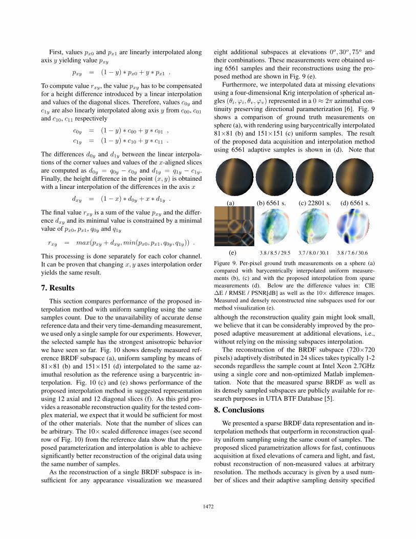
Furthermore, we interpolated data at missing elevations

using a four-dimensional Krig interpolation of spherical an-

gles (θi, ϕi, θv, ϕv) represented in a 0 ≈ 2π azimuthal con-

tinuity preserving directional parameterization [6]. Fig. 9

shows a comparison of ground truth measurements on

sphere (a), with rendering using barycentrically interpolated

81×81 (b) and 151×151 (c) uniform samples. The result

of the proposed data acquisition and interpolation method

using 6561 adaptive samples is shown in (d). Note that

(a) (b) 6561 s. (c) 22801 s. (d) 6561 s.( ) ( ) ( )

(e) 3.8 / 8.5 / 29.5 3.7 / 8.0 / 30.1 3.8 / 7.6 / 30.6

Figure 9. Per-pixel ground truth measurements on a sphere (a)

compared with barycentrically interpolated uniform measure-

ments (b), (c) and with the proposed interpolation from sparse

measurements (d). Below are the difference values in: CIE

ΔE / RMSE / PSNR[dB] as well as the 10× difference images.

Measured and densely reconstructed nine subspaces used for our

method visualization (e).

although the reconstruction quality gain might look small,

we believe that it can be considerably improved by the pro-

posed adaptive measurement at additional elevations, i.e.,

without relying on the missing subspaces interpolation.

The reconstruction of the BRDF subspace (720×720

pixels) adaptively distributed in 24 slices takes typically 1-2

seconds regardless the sample count at Intel Xeon 2.7GHz

using a single core and non-optimized Matlab implemen-

tation. Note that the measured sparse BRDF as well as

its densely sampled subspaces are publicly available for re-

search purposes in UTIA BTF Database [5].

8. ConclusionsWe presented a sparse BRDF data representation and in-

terpolation methods that outperform in reconstruction qual-

ity uniform sampling using the same count of samples. The

proposed sliced parametrization allows for fast, continuous

acquisition at fixed elevations of camera and light, and fast,

robust reconstruction of non-measured values at arbitrary

resolution. The methods accuracy is given by a used num-

ber of slices and their adaptive sampling density specified

147014701472

(a) reference (b) uniform sampl. (c) slices interp. (d) uniform sampl. (e) slices interp.518 400 samples 576 samples 576 samples 2 304 samples 2 304 samples

(f) 1.7 / 4.6 / 34.9 / 0.99 0.9 / 3.2 / 38.2 / 0.99 0.8 / 2.1 / 41.6 / 0.99 0.3 / 0.6 / 52.2 / 1.00

Figure 10. The reference BRDF subspace 720×720 (a) compared with the same size barycentric interpolations from two densities of

uniform sampling 24×24 (b) and 48×48 (d), and the proposed interpolation from the sparse representation using the same samples count

(c) and (e), using thresholds t = 0.47 and t = 0.054, respectively. Below are the 10× difference images and difference values in: CIE

ΔE / RMSE / PSNR[dB] / SSIM. Bottom-left: the proposed uniform placement of measured slices.

by maximal allowed error. We believe that the proposed

data-driven sampling together with the robust reconstruc-

tion performance represents an initial framework for intelli-

gent adaptive sampling methods of view- and illumination-

dependent material appearance.

Acknowledgements – This work has been supported

by the Czech Science Foundation grants P103/11/0335,

P202/12/2413 and EC Marie Curie ERG 239294.

References[1] K. Dana. BRDF/BTF measurement device. In ICCV 2001,

volume 2, pages 460–466, July 2001.

[2] J. Filip and R. Vavra. Fast method of sparse acquisition and

reconstruction of view and illumination dependent datasets.

To appear in Computer and Graphics, page 12, 2013.

[3] M. Fuchs, V. Blanz, H. P. Lensch, and H.-P. Seidel. Adaptive

sampling of reflectance fields. ACM Trans. Graph., 26(2):1–

18, June 2007.

[4] A. Ghosh, S. Achutha, W. Heidrich, and M. O’Toole. BRDF

acquisition with basis illumination. ICCV 2007, 0:1–8.

[5] M. Haindl, J. Filip, and R. Vavra. Digital material appear-

ance: the curse of tera-bytes. ERCIM News, No. 90, pages

49–50, 2012.

[6] V. Havran, J. Filip, and K. Myszkowski. Bidirectional texture

function compression based on the multilevel vector quanti-

zation. Comp. Graph. Forum, 29(1):175–190, 2010.

[7] M. Holroyd, J. Lawrence, and T. Zickler. A coaxial opti-

cal scanner for synchronous acquisition of 3D geometry and

surface reflectance. ACM Tran. Graph., 29:1–12, 2010.

[8] A. Hope, T. Atamas, D. Hunerhoff, S. Teichert, and K.-

O. Hauer. Argon3: 3D appearance robot-based goniore-

flectometer at PTB. Review of Scientific Instruments,

83(4):045102, 2012.

[9] J. Lawrence, S. Rusinkiewicz, and R. Ramamoorthi. Adap-

tive numerical cumulative distribution functions for efficient

importance sampling. In Eurographics Symposium on Ren-dering, pages 11–20, 2005.

[10] J. Lu and J. Little. Reflectance function estimation and shape

recovery from image sequence of a rotating object. In ICCV1995, pages 80–86, 1995.

[11] S. R. Marschner, S. H. Westin, E. P. F. Lafortune, and K. E.

Torrance. Image-based bidirectional reflectance distribu-

tion function measurement. Applied Optics, 39:2592–2600,

2000.

[12] W. Matusik, H. Pfister, M. Brand, and L. McMillan. A data-

driven reflectance model. ACM Trans. Graph., 22(3):759–

769, 2003.

[13] G. Muller. Data-Driven Methods for Compression and Edit-ing of Spatially Varying Appearance. Dissertation, Univer-

sitat Bonn, Dec. 2009.

[14] A. Ngan, F. Durand, and W. Matusik. Experimental analysis

of BRDF models. Eurographics Symposium on Rendering2005, 2:117–126, 2005.

[15] F. Nicodemus, J. Richmond, J. Hsia, I. Ginsburg, and

T. Limperis. Geometrical considerations and nomenclature

for reflectance. NBS Monograph 160, National Bureau ofStandards, U.S. Dept. of Com., pages 1–52, 1977.

[16] J. Robinson. Image coding with ridge and valley primitives.

IEEE Trans. on Communic., 43(6):2095–2102, 1995.

[17] M. Sattler, R. Sarlette, and R. Klein. Efficient and realistic

visualization of cloth. In Eurographics Symposium on Ren-dering 2003, pages 167–178, 2003.

[18] S. K. Thompson and G. A. F. Seber. Adaptive Sampling.

John Wiley and sons, New York, 1996.

147114711473