A front-tracking algorithm for accuraterepresentation of surface tensionStephane Popinet and Stephane ZaleskiModelisation en Mecanique, CNRS URA 229,Universite Pierre et Marie Curie, 4 place Jussieu75005 Paris, France. zaleski@lmm.jussieu.frAbstractWe present a front-tracking algorithm for the solution of the 2Dincompressible Navier-Stokes equations with interfaces and surfaceforces. More particularly, we focus our attention on obtaining anaccurate description of the surface-tension terms and the associatedpressure jump. We consider the stationary Laplace solution for a bub-ble with surface tension. A careful treatment of the pressure gradientterms at the interface allows us to reduce the spurious currents to ma-chine precision. Good results are obtained for the damped oscillationsof a capillary wave compared with the initial-value linear theory. Aclassical test of Rayleigh-Taylor instability is presented.Keywords: drops and bubbles, surface tracking, front tracking, interfaces,surface tension, capillary waves.1 IntroductionA number of methods have been developed in recent years for the solution ofproblems involvingmoving interfaces in multiphase uid ow. These methodscan be divided into two main classes depending on the type of grids used[20, 10, 33, 32]. In the rst class, the interface is treated as a boundarybetween elementary domains. This approach allows a precise representationof the interfacial jumps conditions, at least in principle. However, it requiresdeformable grids in order to follow the motion of the interface [11, 12]. Thesecond class of methods uses xed grids to describe the velocity eld but1

requires specic advection schemes in order to preserve the sharpness ofthe interfacial front. These advection schemes may in turn be divided intotwo groups, either implicitly or explicitly representing the interface. Theimplicit methods are sometimes labeled front-capturing in analogy with thesituation in computational gas dynamics, while the explicit methods are oftencalled front-tracking. Among the implicit methods are Volume Of Fluid andLevel Sets. Modern Volume Of Fluid (VOF) advection schemes yield goodresults and ensure an accurate conservation of mass [2, 19, 30]. Level-setmethods are easy to implement and are similar in their properties to volumeof uid methods [34]. Both rely on an implicit description of the interface,given through phase functions (i.e. volume fraction for the VOF method ordistance function for the level-set method). In the second group, trackingmethods such as interfacial markers uses a more explicit discretization of theinterfacial discontinuity. They are somewhat more complex to implement,but give the precise location and geometry of the interface [35, 36].All these methods provide good solutions to the problem of interfaceadvection; however, accurate representation of surface forces (i.e. surfacetension, membrane eects, . . . ) remains a problem when using xed grids.A striking feature of these methods (including lattice gases [31]) are the so-called spurious currents shown in gure 1. These numerical artifacts resultFigure 1: Spurious currents around a stationary bubble. The method usedfor the interface advection is a VOF scheme.from inconsistent modeling of the surface tension terms and the associatedpressure jump. In some case they may lead to catastrophic instabilities in2

interface calculations. More generally, this poses the problem of obtainingan accurate description of the steep gradients occurring at the interface.These problems are often compounded by the presence of high densityratios. Many multiphase ow problems of interest involve uids with veryhigh ratios of densities and viscosities simply because mixtures of liquids andgases are the most common uids composing multiphase ows. Thus experi-ments often involve air bubbles in water, water droplets in air, wave breakingetc. which are dicult or impossible to address with current multiphase owcomputational techniques. Moreover, with such uids, surface tension eectsare usually large compared to viscous damping. In these cases, the eect ofthe unbalanced forces acting on the interface not only reduces the accuracybut can lead to spurious currents [16] which create oscillations strong enoughto destroy the interface. The spurious currents are therefore more than justa numerical inaccuracy but are a real limitation of methods used on xedgrids.In this paper, we present a front-tracking method for the solution ofthe two-dimensional incompressible Navier-Stokes equations with interfacesand surface eects. We will more particularly investigate the accuracy ofthe numerical representation of the surface tension and of the associatedpressure jump. In the section which follows, we describe the general schemeused to solve the Navier-Stokes equations. The second section gives a detaileddescription of the front tracking algorithm and in the nal section, some testcases investigating the numerical accuracy and convergence properties arepresented.2 General description of the method2.1 Basic equationsWe seek to solve the incompressible Navier-Stokes equations with varyingdensity and surface tension. The momentum and mass-balance equationsare (@tu+ u ru) = rp+r (2D) + sn+ g (1)r u = 0: (2)The former may be written in conservative form@u@t +r (u u) = rp+r (2D) + sn+ g; (3)where u = (u; v) is the uid velocity, = (x; t) is the uid density, = (x; t) is the uid viscosity, D is the rate of deformation tensor with3

components Dij = (@iuj+@jui)=2. The surface tension term is considered tobe a force concentrated at the interface, is the surface tension coecient, the curvature of the interface, s a distribution concentrated on the interfaceand n is the unit normal to the interface. In the case of two immiscible uids,we may dene a characteristic function which is equal to 1 in phase 1 and 0in phase 2. Then and n are related by r = ns . In the absence of phasechange simply follows the uid motion and thus satises the advectionequation @@t + u r = 0: (4)Density and viscosity are attached to the phases and thus can be expressedas functions of = 1 + (1 )2 (5) = 1 + (1 )2: (6)Alternately, the equations of motion may be written in jump condition form.Jump conditions appear when one investigates eqs. (1) or (3) in the neighbor-hood of the singular surface S. This leads to the tangential stress condition[t D n]S = 0; (7)where the notation [:]S represents the jump of a quantity across the surfaceS. We also obtain from (1) or (3) the normal stress condition[n (pI+ 2D) n]S = ; (8)while the usual assumption of continuity of velocity leads to[u]S = 0: (9)Away from the interface eq. (1) takes the usual form (@tu+ u ru) = rp+ r2u: (10)The normal stress condition (8) leads to the famous Laplace law for a spher-ical interface of radius R in undeformed ow:[p]S = 2R : (11)4

Ci,j

Pi,j

Vi,j+1/2ρ

Vi,j-1/2ρ

ρUi-1/2,j ρ Ui+1/2,jFigure 2: MAC discretization of the pressure, volume fraction, momentumand velocity componentsx y

ρ Pi,j

Ci,j

Pi,jCi,j

ρ

ρ

ρ

ρ

ρ

ρ

Ω Ω

Ui+1/2,j

Vi,j+1/2

Vi,j-1/2

Ui-1/2,j ρUi-1/2,j Ui+1/2,j

Vi,j+1/2

Vi,j-1/2Figure 3: Control volumes for the u and v momentum components5

2.2 The Navier-Stokes solverWe use a momentum-conserving formulation of the Navier-Stokes equation.The solution technique is close to the one initially developed for the SURFERcode [16]. It is based on an explicit projection method [23]. The pressure,volume fraction, momentum and velocity components are discretized on auniform Cartesian mesh (x = y = h) using a staggered Marker And Cell(MAC) [23] distribution (gure 2). If we associate the control volumes xand y of gure 3, to the components u and v of the momentum, we canwrite the integral of (3)@@t Z udx = L(u; ) I@ pdS (12)whereL(u; ) = I@ u u dS + I@ 2D dS+ Z sndx+ Z gdx: (13)Actually equation (13) is projected on the x-direction (resp. y) for the x(resp. y) control volumes. We denote these control volumes with halfinteger indices, so x = i+1=2;j, y = i;j+1=2. (In all these expressions i; jare integers.) This allows us to dene momentum variables centered on therelevant cells (ux)i+1=2;j = 1jj Zi+1=2;j uxdx (14)where jj = h2 is the measure of the control volume . Similarly controlvolumes centered on the pressure nodes have the form ij. The discrete for-mulation of (12) is then obtained by straightforward approximations of andu at the center of the faces of the control volumes x and y. Interpolationsare performed as required. The values of and near the interface are ob-tained by an approximation of the characteristic function by the volumefraction Cij = Zij dx (15)with i; j integer or half-integer. Then we approximate eqs. (5) and (6) byij = Cij1 + (1 Cij)2 (16)ij = Cij1 + (1 Cij)2: (17)The discretization of the surface tension term R sndx, which is the maintopic addressed in this paper, will be described separately in the next ses-sion. First we give an outline of our explicit projection method. It can besubdivided into four steps: 6

1. The interface is advected using the velocity eld at time tn = n where is the time step. In our case this is done using a Lagrangian advectionof the markers. This denes the approximation of characteristic func-tion n+1 at time tn+1. The volume fraction may then be computed byquadrature.2. A provisional solution (u)? of the momentum at time (n+1) is builtusing an explicit discretization of (12)(u)? = (u)n + L(un; Cn+1) (18)where n is the value of the function at time n , L is a discretizationof the operator in eq. (13) and we approximate by C. A detaileddescription of this step may be found in [13].3. We then ensure the divergence-free character of the velocity eld un+1.From eq. (13) the eect of pressure on the momentum balance is(ux)n+1i+1=2;j = (ux)?i+1=2;j jj Ii+1=2;j pdS: (19)It is useful at this point to dene the velocity elds in terms of themomentum eldsu?x;i+1=2;j = (ux)?i+1=2;j=n+1; un+1x;i+1=2;j = (ux)n+1i+1=2;j=n+1; (20)with a similar denition for the y elds. Equation (19) can thus bere-expressed in terms of the velocity eldsun+1 = u? n+1jj Ii+1=2;j pdS (21)We want to satisfy the continuity equation in the formr un+1 = 0 (22)at each point xi;j. This impliesr ( n+1jj Ii+1=2;j pdS) = r u?: (23)Discretizing as before on the MAC staggered grid, this leads to thePoisson-like equation for the pressurerh ( n+1rhp(n+1)) = rh u?: (24)7

where the rh operator is the centered nite-dierence operator on thestaggered grid dened asrhpx;i+1=2;j = 1h (pi+1;jpi;j); rhpy;i;j+1=2 = 1h(pi;j+1pi;j): (25)Although we use eq. (24) in the bulk, near the interface we need amore accurate discretization of (23) which will be discussed in section3.6 below. This equation is solved eciently using a multigrid solver[6, 7, 25, 38].4. The momentum and velocity elds at time (n + 1) are computed byequation (19).2.3 Interface and surface tensionA

Ω

Ut

tB

A

B

ρFigure 4: In the \method of tensions" the contribution of the surface tensionto the momentum equation is obtained as the sum of two vectors tangent tothe interface. First the direction of the vectors is determined from a splinerepresentation of the interface, then the sum of the two tangent vectors times is added to the momentum balance of the cell.Given a parametric description (x(s); y(s)) of the location of the interface,where s is the arc-length, we want to compute the source term due to thesurface tension in the momentum equation (13). If is the control volumefor one of the components of the momentum and AB, the interface segmentinside this control volume (gure 4), the integral source term in (13) isZ sndx = I BA nds; (26)which can be written using the rst Frenet's formula for parametric curves I BA nds = I BA dt = (tB tA) (27)8

where t is the oriented unit tangent to the curve. The integral source termdue to the surface tension is then the sum of the outward unit tangents atthe points where the interface enters or exits the control volume.3 Front-tracking algorithmIn this section, we present a detailed description of the front-tracking algo-rithm. The interface is represented using an ordered list of marker particles(xi; yi), 1 i N . A list of connected polynomials (pxi (s); pyi (s)) is con-structed using the marker particles and gives a parametric representationof the interface, with s an approximation of the arc-length. Both lists areordered and thus identify the topology of the interface.3.1 Advecting the pointsThe rst step in our algorithm is the advection of the marker particles. Weuse a simple bilinear interpolation to nd the velocity inside cell i;j+1=2u(x; y) = ui1=2;j(1 x y + xy) + ui+1=2;jx(1 y) + (28)ui1=2;j+1y(1 x) + ui+1=2;j+1xy;where x and y are the coordinates of the point relative to the (i 1=2; j)vertex. (Here and in the remainder of sec. 3 we rescale lengths so thath = 1.) The marker particles are then advected in a Lagrangian mannerusing a straightforward rst-order explicit schemexn+1i = xni + u(xni ; yni ) (29)yn+1i = yni + v(xni ; yni ):Once the points have been advected we need to reconstruct the parametricrepresentation of the interface.3.2 Constructing the polynomialsWe have chosen to use connected cubic polynomials with continuous rst andsecond-order derivatives. This type of curve is usually known as cubic splines[37, 15, 24]. The parametric representation is often periodic as the interfacesare mostly self-connected (drops, bubbles, periodic wave trains . . . ).We then need to choose a parameter s in order to interpolate the twosets of points (xi; si) and (yi; si). A simple choice is an approximation of the9

arclength si = i1Xj=1 h(xj+1 xj)2 + (yj+1 yj)2i1=2 : (30)The connection conditions for the interpolating polynomials lead to twopseudo tridiagonal systems Ba = c, one for each coordinate of the para-metric curve, where B is a N2 matrix of the formB = 0BBBBBBB@ b1 c1 0 0 a1a2 b2 c2 0 00 . . . . . . . . . 00 0 aN1 bN1 cN1cN 0 0 aN bN 1CCCCCCCA (31)where the coecients a1 and cN arise from the periodicity condition [15].The solution of this type of system can be reduced to the solution of twotridiagonal systems which are easily solved using classical techniques [24].Thus, the construction of the interpolating parametric spline curve from theset of points (xi) requires the solution of four tridiagonal systems of size N2.This can be done in O(N) operations. All the other operations of our markeralgorithm deal with local computations along the interface. They are thusalso of order N . The ratio between the time spent in the marker algorithmand in the computations done on the bulk of the uid (the Navier-Stokessolver) is then of order 1=N . As the domain size increases the proportionof computational time needed by the marker representation decreases. Inpractice, the marker computation accounts for less than 10 % of the time fora 642 mesh.3.3 RedistributionAs the interface evolves, the markers drift along the interface following tan-gential velocities and we may need more markers if the interface is stretchedby the ow. We then need to redistribute the markers in order to ensurean homogeneous distribution of points along the interface. This is done ateach time step using the interpolating curve (x(s); y(s)). As s is an ap-proximation of the arclength, if we choose a redistribution length l, thenew number of markers is Nnew = sN=l and the points are redistributedas (xnewi ; ynewi ) = (x(il); y(il)). l is usually chosen as h, which yields an av-erage number of one marker per computational cell. Decreasing this lengthdoes not apparently improve the accuracy and in some cases leads to instabil-ities. This is similar to the behavior of boundary integral codes that also usearclength parameterization, cubic splines and redistribution of nodes [21].10

3.4 Estimation of the volume fractionIn the case of ows with varying density and/or viscosity between the phases,we need to estimate the volume fraction C dened in eq. (15). We then haveto create the new volume fraction eld corresponding to the new parametricinterpolation of the interface. This is performed as described in Appendix B.3.5 Surface tension contribution to the momentum equa-tionFollowing the tension formulation (27), if the interface crosses a momen-tum control-volume boundary, we compute the value of the parameter s(using the same procedure as above) for the intersection point. We thenadd the relevant component of surface tension contribution t where t isthe unit tangent to the curve pointing outward for the considered cell: t =(x0(s); y0(s))=(x02(s) + y02(s))1=2. As this computation is done once for thetwo neighboring cells, the contributions of surface tension to the global mo-mentum cancel to machine accuracy. Thus the sum of surface tension forcesover a droplet or bubble is zero, even if there are errors for the surface tensionin a single cell.3.6 Pressure gradient correctionFor our staggered grid, the x-component of the integral contribution of thepressure gradient is given by H@ pdS = h(pi;jpi1;j). For instance, consideran interface crossing the vertical face BC of the control volume (g. 5).There is a pressure jump either between pi;j and pi;j1 (case (a): EB < h=2),or between pi;j and pi;j+1 (case (b): EB > h=2). We can have a betterapproximation of the integral R CB pdS using the nearest pressure nodes if EB < h=2: RCB pdS = EBpi;j1 + ECpi;j. if EB h=2: R CB pdS = EBpi;j + ECpi;j+1.This can be viewed as a correction to the standard centered estimate. Dene if EB < h=2: Ii;j[p] = EB(pi;j1 pi;j). if EB h=2: Ii;j[p] = (h EB)(pi;j+1 pi;j).Then R CB pdS = hpi;j + Ii;j[p]: Ideally, this \pressure-gradient correction"should be applied when solving the pressure equation (23). This would lead11

Pi,j

Pi,j+1

Pi-1,j

B

C

Pi,j

Pi,j-1

Pi-1,j

B

E

C

(a) (b)

Ui-1/2,jρ Ui-1/2,jρ E

Figure 5: The pressure gradient correction for a MAC grid. The location ofthe interface relative to the pressure nodes yields two cases: (a): EB < h=2,(b): EB > h=2.to a discretization of (23) in the formrh n+1rh(p(n+1) + I[pn+1]) = rh u?: (32)We have chosen a simpler approach, however, where the pressure gradientcorrection is considered as a source term in the right-hand side of the mo-mentum balance equation (13):rh n+1rhp(n+1) = rh n+1rhI[p(n)] +rh u?: (33)This term is then computed using the pressure eld at time n . This isdone in practice when computing the surface-tension contribution which alsorequires the intersection point E. (It is less accurate to use (33) instead of(32) but justied as the method gives good results for dicult test cases.)This pressure gradient correction is probably the simplest choice available.However several other solutions exist and it would be interesting to assesstheir accuracy and convergence properties. A simple extension is the choice ofhigher order interpolation schemes on both sides of the interface. The meansquare interpolation proposed by Shyy et al. [33] would also be applicable andcould be used to obtain any term with rapid variations across the interface(e.g. viscous terms for high contrasts of viscosity).12

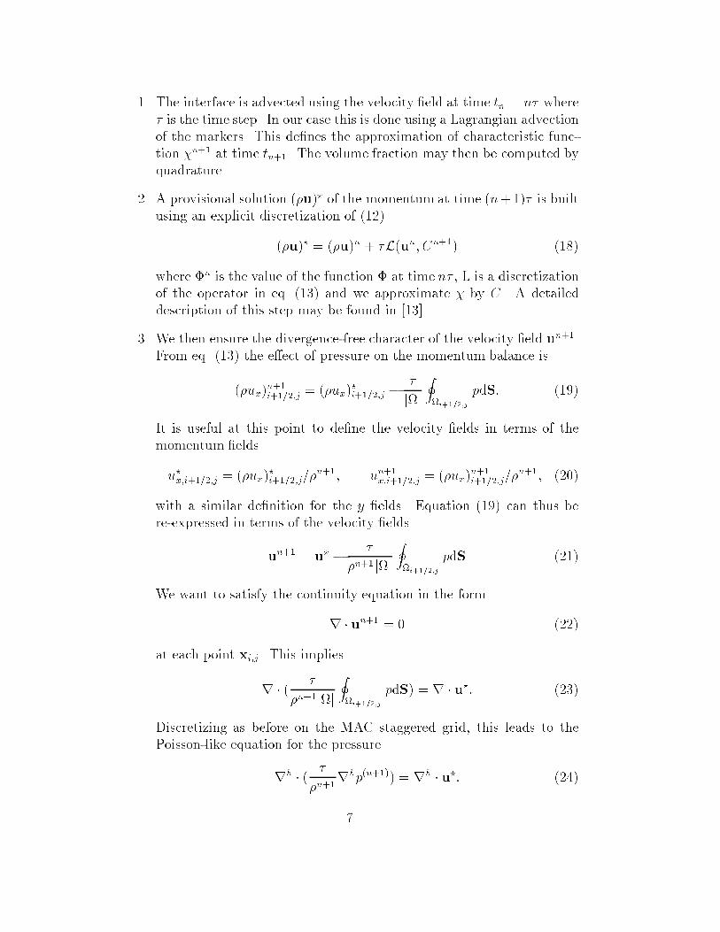
4 ResultsIn this section, we present some simple test cases intended to illustrate theability of our method to cope with high surface-tension ows without lossof accuracy. All the computations have been done on an IBM RS6000/370workstation. Typically one time step on a 1282 grid requires 0.7 second, themost time-consuming procedure being the multigrid solver.4.1 Stationary bubble and spurious currentsAn interesting test case is the verication of the stationary Laplace solutionfor a circular bubble or droplet. As shown previously, in principle a stationarysolution exists for our method and consequently Laplace's law should beveried exactly. However, one cannot interpolate a circle (which is C1)exactly using a parametric spline curve (C2 in our case) and small dierenceswill subsist. Two questions follow, the stability of this approximate solutionand its numerical convergence to the theoretical solution.In the absence of externally imposed velocity, the relevant dimensionlessnumbers are the Ohnesorge number Oh = =(D)1=2, (or the less-often usedLaplace number La = 1=Oh 2) and the ratios 1=2 and 1=2. When nu-merical simulations are performed, spurious currents of amplitude U are ob-served. In [16] it was conjectured that the amplitude of the spurious currentsmust be proportional to =. This is equivalent to having an approximatelyconstant value of the capillary number Ca s = U=.The Reynolds number UD= of the spurious currents is then propor-tional to La = D=2. When La is large, computations become dicultin our previous scheme [16] because the spurious currents develop a kindof turbulence, shaking the droplet in a kind of Zitterbewegung. However,in our new scheme with pressure correction, we observe two interesting fea-tures. First there is remarkable constancy of Ca s with Oh , indicating thatspurious currents are very predictable. Second we can reach high values of1=Oh 2 which was not previously possible. The nal bonus is that increasingthe resolution at xed Oh makes the spurious currents decrease to machineaccuracy.Table 1.a illustrates the constant character of Ca over a broad range ofOhnesorge numbers. We used a 322 Cartesian mesh with periodic boundaryconditions in the x direction and re ecting conditions on the horizontal walls,the density and viscosity ratios are one, the ratio between the diameter andthe box width is 0.4. We measured the maximum amplitude of the spuriouscurrents after 250 characteristic time scales (t = tphys=(D) = 250). Asecond series of tests was performed with the same geometry, for a value13

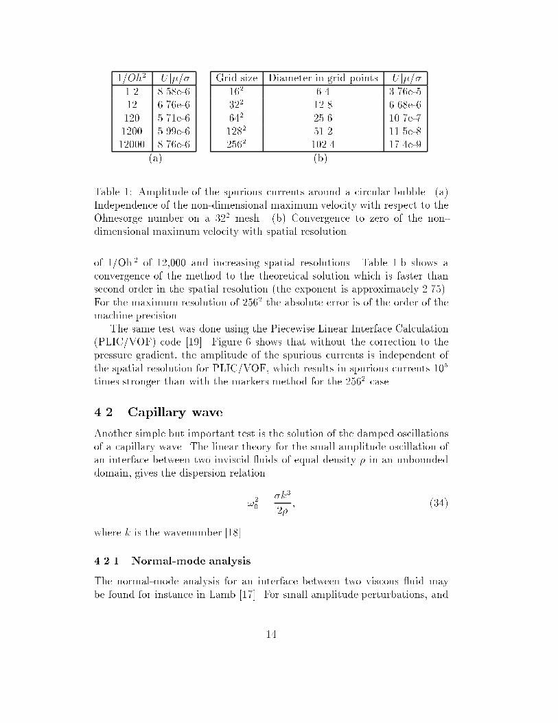
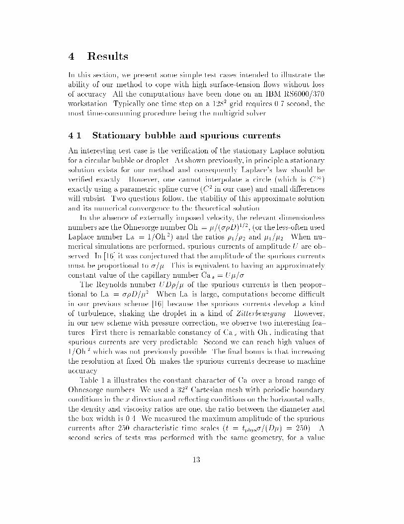
1=Oh2 jU j=1.2 8.58e-612 6.76e-6120 5.71e-61200 5.99e-612000 8.76e-6 Grid size Diameter in grid points jU j=162 6.4 3.76e-5322 12.8 6.68e-6642 25.6 10.7e-71282 51.2 11.5e-82562 102.4 17.4e-9(a) (b)Table 1: Amplitude of the spurious currents around a circular bubble. (a)Independence of the non-dimensional maximum velocity with respect to theOhnesorge number on a 322 mesh. (b) Convergence to zero of the non-dimensional maximum velocity with spatial resolution.of 1=Oh 2 of 12,000 and increasing spatial resolutions. Table 1.b shows aconvergence of the method to the theoretical solution which is faster thansecond order in the spatial resolution (the exponent is approximately 2.75).For the maximum resolution of 2562 the absolute error is of the order of themachine precision.The same test was done using the Piecewise Linear Interface Calculation(PLIC/VOF) code [19]. Figure 6 shows that without the correction to thepressure gradient, the amplitude of the spurious currents is independent ofthe spatial resolution for PLIC/VOF, which results in spurious currents 105times stronger than with the markers method for the 2562 case.4.2 Capillary waveAnother simple but important test is the solution of the damped oscillationsof a capillary wave. The linear theory for the small amplitude oscillation ofan interface between two inviscid uids of equal density in an unboundeddomain, gives the dispersion relation!20 = k32 ; (34)where k is the wavenumber [18].4.2.1 Normal-mode analysisThe normal-mode analysis for an interface between two viscous uid maybe found for instance in Lamb [17]. For small amplitude perturbations, and14

0.0 20.0 40.0 60.0 80.0 100.0Diameter in grid points

10−8

10−7

10−6

10−5

10−4

10−3

10−2

|U|m

u/si

gma PLIC

Markers

Figure 6: Amplitude of the spurious currents versus spatial resolution for thePLIC method without pressure correction and the current method.15

when the viscosities and densities of both uids are the same we have thedispersion relation !2 = k32 (1 k=q) = !20(1 k=q); (35)where q = qk2 i!=: (36)which gives the viscous correction to the inviscid case (34) and the dampingratio of the amplitude. Eliminating ! between (35) and (36) one nds thatq is a root of the quartic equationq(q k)(q + k)2 = k322 ; (37)which can be solved numerically.4.2.2 Initial-value problemAs will be shown from the numerical simulations, this normal-mode analysisis not suitable for the study of the related initial-value problem. As shownby Prosperetti et al. [8, 26], an analytical solution (given in Appendix B)exists for the initial-value problem in the case of the small-amplitude waveson the interface between two superposed viscous uids, provided the uidshave the same dynamic viscosity.4.2.3 Comparison with the numerical simulationsThe test case for the capillary wave is a square box divided in two equalparts by a sinusoidal perturbation. The wave length is equal to the boxwidth. The boundary conditions are free slip on the top and bottom walls,periodic along the horizontal axis. The ratio between the initial interfaceperturbation H0 and the box height is 0.01. We let Oh = 1=p3000 thenon dimensional viscosity = k2=!0 6:472 102, and the two uidsdensities are the same. Figure 7 shows the evolution of the amplitude withtime for the numerical solution and both the normal-mode and initial-valueanalytical solutions. The normal-mode curve is obtained using H0ei!t0=!0where ! is given by eq. (35).In order to study the spatial convergence of the method, we have repeatedthis test for resolutions of 82, 162, 322 and 642. Table 2 summarizes theresults. We obtain a good convergence and a relative error of order 102 from16

0.0 10.0 20.0Non dimensional time

−0.010

−0.005

0.000

0.005

0.010

Rel

ativ

e am

plitu

de

Front trackingInitial valueNormal mode

−0.10

−0.05

0.00

0.05

0.10

Rel

ativ

e er

ror

Figure 7: Time evolution of the amplitude of a capillary wave in the vis-cous case. Our front-tracking method is used on a 1282 square grid. Thetheoretical curves are obtained from a normal-mode analysis and from theexact solution to the initial-value problem in the linearized viscous case (seeAppendix B). 17

0.0 2.0 4.0Non dimensional time

−0.010

0.000

0.010R

elat

ive

ampl

itude

Front trackingInitial valueNormal mode

Figure 8: Close up of the previous gure illustrating the dierence betweenthe normal-mode and initial-value solutions.Grid size Error/Initial value Error/Normal mode82 0.2972 0.3077162 0.0778 0.0959322 0.0131 0.0332642 0.0098 0.03071282 0.0065 0.0280Table 2: Evolution of the relative error between numerical computations andthe normal-mode and initial-value analytical solutions. The relative error isthe r.m.s. of the dierences between the solutions divided by the amplitudeof the initial perturbation. We compare the solutions for the rst 25 non-dimensional time units. 1 = 2, non-dimensional viscosity 6:472 102,Oh = 1=p3000. 18

Grid size Error/Initial value82 0.3593162 0.1397322 0.0566642 0.02641282 0.0148Table 3: Evolution of the relative error between numerical computations andthe initial-value analytical solution. 1 = 102, 4:799 102, Oh 1 =1=p3000, Oh 2 = 1=p30000.a spatial resolution of 322 compared to the initial-value analytical solutionof Prosperetti. Moreover, we treat here the case of a bounded domain ofaspect ratio h= = 1=2 where h is the half height of the computationalbox and = 2=k the wavelength. The analytical solution is given in theinnite depth case and should be corrected with a term of order cotanh(kh) =cotanh 1:0037.The previous test was performed with a density ratio of one. Table 3illustrates the results for a density ratio of ten.4.3 Rayleigh-Taylor instabilityIn order to illustrate the capability of our method to deal with more complexcases, we present here a classical test. The original version of this computa-tion has been performed by Puckett et al. [29, 30] using a VOF type method.A one-meter wide, four-meters high rectangular domain is discretized usinga 64 256 grid. The uid densities are 1.225 and 0.1694 kg=m3. The uidviscosities are 0.00313 kg:m1:s1. The interface between the uids is an ini-tially sinusoidal perturbation of amplitude 0:05 meters. Figure 9 shows theevolution of the interface at times 0, 0.7, 0.8 and 0.9 seconds. The maximummass uctuation of our method is approximately 0:14%, which is larger thanthe observed variation for a VOF-type method (about 0:01%). The interfaceevolution compares well with the results of Puckett et al. [29] and with thesimulation done using the VOF/PLIC algorithm of ref. [19] on a 128 512grid (gure 10). 19

t=0.9t=0.7t=0.0 t=0.8Figure 9: Rayleigh-Taylor instability on a 64 256 grid using the front-tracking algorithm.20

t=0.9t=0.7t=0.0 t=0.8Figure 10: Rayleigh-Taylor instability on a 128 512 grid using theVOF/PLIC algorithm.21

5 ConclusionsIn summary, we have presented a front-tracking numerical algorithm able todeal accurately with surface tension. For the case of a stationary bubble, themethod shows a convergence to the theoretical solution which is faster thansecond order in the spatial resolution. For reasonable mesh sizes, the spuriouscurrents usually present when using xed grids can then be reduced to ma-chine accuracy. Good results are obtained for the test case of a capillary wavewith viscous damping. We obtain very good agreement with Prosperetti'ssolution to the linearized initial-value problem. The relative error for thetime evolution of the amplitude is smaller than 102 when using 32 or morepoints per wavelength. The method is robust and remains accurate even forvery small Ohnesorge numbers (103 or less). The implementation of themethod leads relatively easily to a fast code: as we use a xed regular grid,the Navier-Stokes algorithm is ecient. Moreover, due to its one-dimensionalnature, the surface-tracking part is negligible in terms of computational time.The marker representation gives a precise location of the interface and istherefore well-suited for the study of small scale eects.We note however, that we have not yet implemented a reconnection mech-anism to deal with topology changes. Consequently, our method conservesthe small lamentary structures even for low resolutions. We are currentlystudying a reconnection mechanism based on a physical representation ofthe short-range interactions between interfaces. Whereas VOF-type meth-ods introduce an arbitrary reconnection length (usually the mesh spacing),this method should provide a physical criterion for the reconnections. Thisadvantage of explicit front-tracking in providing a potentially better answerto the reconnection problem was recognized in ref. [36].The main idea of this paper is to take into account the fact that theinterface is a sharp discontinuity when building the surface tension represen-tation. This idea could be generalized to include the other singularities ofthe equation, of which the most prominent example is the jump in density.It remains to be seen whether such an improvement will be as easy to obtainas in the case of surface tension.An interesting comment on our approach is that it runs counter to severalattempts to deal with singularities in the equations by smoothing them, i.e.distributing them over neighboring mesh nodes through appropriate smooth-ing kernels [36, 5, 1].The ideas developed in this paper can be generalized to dierent types ofNavier-Stokes solvers and are not limited to projection methods on Cartesiangrids. In particular, we emphasized the necessity of a precise and consistentdiscretization of the surface tension and of the associated pressure jump.22

This requires the precise knowledge of the interface position relative to theunderlying grid that front tracking usually provides.It is important to note that this approach could be and should be appliedto the discretization of all the gradient terms with rapid variations across theinterface, in particular the viscous stress tensor for high viscosity contrasts.Numerous applications require an accurate representation of the surfaceeects: motion of drops of water in air [39, 28], wave breaking [3] or sono-luminescence [27]. Moreover, the exact description of the interface positionallows an easy implementation of the membrane models found in biologicalmechanics [4, 14] and of the eect of surfactants [22]. An interesting studycould also be a detailed sub-grid modeling of the reconnections between in-terfaces [9].We are currently working on an axisymmetric version of the code. In thefuture, we plan to develop a fully three-dimensional front-tracking algorithm.References[1] I. Aleinov and E. G. Puckett. Computing surface tension with high-order kernels. In K. Oshima, editor, Proceedings of the 6th Interna-tional Symposium on Computational Fluid Dynamics, pages 613, LakeTahoe, CA, 1995. May be obtained from the author's web page athttp://math.math.ucdavis.edu/ puckett/.[2] N. Ashgriz and J. Y. Poo. FLAIR: Flux line-segmentmodel for advectionand interface reconstruction. J. Comput. Phys., 93:449468, 1991.[3] M. L. Banner and D. H. Peregrine. Wave breaking in deep water. Ann.Rev. Fluid Mech., 25:373, 1993.[4] D. Barthes-Biesel. Microrheological models of red blood cell mechanics.Advances in Hemodynamics and Hemorheology, 1:3165, 1996.[5] J.U. Brackbill, D. B. Kothe, and C. Zemach. A continuum method formodeling surface tension. J. Comput. Phys., 100:335354, 1992.[6] A. Brandt. Guide to multigrid development. Multigrid Methods,Springer Verlag, Berlin, 1982.[7] W. L. Briggs. A multigrid tutorial. SIAM Philadelphia, 1987.[8] L. Cortelezzi and A. Prosperetti. Small amplitude waves on the surfaceof a layer of a viscous liquid. Quaterly Appl. Math., 38:375388, 1981.23

[9] Jens Eggers. Universal pinching of 3D axisymmetric free-surface ow.Phys. Rev. lett., 71:34583461, 1993.[10] J. M. Floryan and H. Rasmussen. Numerical methods for viscous owwith moving boundaries. Appl. Mech. Rev., 42:323340, 1989.[11] D. E. Fyfe, E. S. Oran, and M. J. Fritts. Surface tension and viscositywith lagrangian hydrodynamics on a triangular mesh. J. Comput. Phys.,76:349384, 1988.[12] J. Glimm, O. McBryan, R. Meniko, and D. H. Sharp. Front trackingapplied to rayleigh-taylor instability. SIAM J. Sci. Stat. Comput., 7:230251, 1987.[13] Denis Gueyer, Jie Li, Ruben Scardovelli, and Stephane Zaleski. Vol-ume of uid interface tracking with smoothed surface stress methodsfor three-dimensional ows applied to pinching threads. in preparation,1997.[14] D. Halpern and T. W. Secomb. The squeezing of red blood cells throughcapillaries with near-minimal diameters. J. Fluid Mech., 203:381400,1989.[15] G. Hammerlin and K. H. Homan. Numerical Mathematics. SpringerVerlag, Berlin, 1991.[16] B. Lafaurie, C. Nardone, R. Scardovelli, S. Zaleski, and G. Zanetti. Mod-elling merging and fragmentation in multiphase ows with SURFER. J.Comput. Phys., 113:134147, 1994.[17] H. Lamb. Hydrodynamics. Cambridge University Press, 1932.[18] L. D. Landau and E. M. Lifshitz. Fluid Mechanics. Pergamon Press,New York, 1959.[19] Jie Li. Calcul d'interface ane par morceaux (piecewise linear interfacecalculation). C. R. Acad. Sci. Paris, serie IIb, (Paris), 320:391396,1995.[20] James Mc Hyman. Numerical methods for tracking interfaces. PhysicaD, 12:396407, 1984.[21] Ali Nadim. private communication.24

[22] Y. Pawar and K. J. Stebe. Marangoni eects on drop deformation in anextensional ow: The role of surfactant physical chemistry. I. Insolublesurfactants. Phys. Fluids, 8:17381751, 1996.[23] R. Peyret and T. D. Taylor. Computational Methods for Fluid Flow.Springer Verlag, New York/Berlin, 1983.[24] W. H. Press, B. P. Flemming, S. A. Teukolsky, and W. T. Vetterling.Numerical Recipes, The Art of Scientic Computing, Second Edition.Cambridge University Press, 1989.[25] W. H. Press and S. A. Teukolsky. Multigrid methods for boundary valueproblems. Computers in Physics, SEP/OCT:514519, 1991.[26] A. Prosperetti. Motion of two superposed viscous uids. Phys. Fluids,24:12171223, 1981.[27] A. Prosperetti. A new mechanism for sonoluminescence. J. Acoust. Soc.Am., 101:20032007, 1997.[28] Andrea Prosperetti and Hasan N. O~guz. The impact of drops on liquidsurfaces and the underwater noise of rain. Annual Reviews of FluidMechanics, 25:577602, 1993.[29] E. G. Puckett, A. S. Almgren, J. B. Bell, D. L. Marcus, and W. J.Rider. A second-order projection method for tracking uid interfaces invariable density incompressible ows. submitted to J. Comp. Phys.[30] E. G. Puckett, A. S. Almgren, J. B. Bell, D. L. Marcus, and W. J. Rider.A high order projection method for tracking uid interfaces in variabledensity incompressible ows. J. Comp. Phys., 100:269282, 1997.[31] D. H. Rothman and S. Zaleski. Lattice-gas cellular automata. CambridgeUniversity Press, Cambridge, UK, 1997.[32] J. A. Sethian. Level Set Methods. Cambridge University Press, 1996.[33] W. Shyy, H.S. Udaykumar, M.M. Rao, and R. W. Smith. Computational uid dynamics with moving boundaries. Taylor and Francis, London,1996.[34] M. Sussman, P. Smereka, and S. Osher. A level set approach for com-puting solutions to imcompressible two-phase ow. J. Comput. Phys.,114:146159, 1994. 25

[35] G. Tryggvason and S. O. Unverdi. Computations of three-dimensionalRayleigh-Taylor instability. Phys. Fluids, 2:656659, 1990.[36] S. O. Unverdi and G. Tryggvason. A front-tracking method for viscous,incompressible, multi- uid ows. J. Comput. Phys., 100:2537, 1992.[37] J. L. Walsh, J. H Ahlberg, and E. N. Nilson. Best approximation prop-erties of the spline t. Journal of mathematics and mechanics, 11:2,1962.[38] P. Wesseling. An introduction to multigrid methods. Wiley, Chichester,1992.[39] S. Zaleski, Jie Li, and S. Succi. Two-dimensional Navier-Stokes simu-lation of deformation and breakup of liquid patches. Phys. Rev. Lett.,75:244247, 1995.

26

Appendix A: estimation of the volume fractionIn the case of ows with varying density and/or viscosity between the phases,we need to estimate the volume fraction C dened in eq. (15). We then haveto create the new volume fraction eld corresponding to the new parametricinterpolation of the interface.Consider a cell crossed by the interface. Phase 1 occupies a subset (gure 11). We wish to compute the volume fraction Cij = jj=jj. Thisproblem can be reduced to the computation of a circulation along a para-metric curve as illustrated below. Following Stokes theorem, if P and Q areD

δΩ

C

B

CijΩ

A

Figure 11: Computation of the volume fractiontwo functions of the space coordinates (x; y) we can writeI@ Pdx+Qdy = Z @Q@x @P@y ! dxdy; (38)if we choose P = 0, Q = x we getI@ xdy = Z dxdy; (39)which can be written using the parametric description of @. We redenex(s); y(s) to follow the sum of the interface S and the \wet" boundary of for s = s1 to s2. Z s2s1 x(s)y0(s)ds = jj: (40)For our third order polynomial parametric function (x(s); y(s)),x(s) = axs3 + bxs2 + cxs+ dxy(s) = ays3 + bys2 + cys+ dy; (41)27

thus the contribution of the interface S to the integral is given byZ sDsA x(s)y0(s)ds = 12axays6 + 15(3bxay + 2axby)s5 +14(axcy + 2bxby + 3cxay)s4 + 13(bxcy + 2cxby + 3dxay)s3 +12(cxcy + 2dxby)s2 + dxcys: (42)where the points sA and sB correspond to the intersections with @ as onthe gure. We must then add the circulation along the faces of the cell. Inthe case of our Cartesian grid, three useful observations can be made:1. As for the horizontal faces R xdy = 0, only the vertical faces contributeto the circulation.2. If a vertical face is not crossed by the interface it contributes R xdy =x R dy = x, which is an integer number.3. We impose a maximum CFL number of 0.5. In this case the variationof the volume fraction during any time step can not be larger than 0.5in any cell. Consequently, we can writecn 0:5 cn+1 cn + 0:5 (43)If we compute only the fractional part of the circulation, ~cn+1, then thesought result is given by cn+1 = ~cn+1 + i, where i is an unknown integer.However i is uniquely dened by (43) and can take only four distinct valuesf1; 0; 1; 2g.It is now easy to compute the volume fraction, we just follow the inter-face, as dened by the list of polynomials. We test whether the interfaceintersects the horizontal and/or vertical grid lines. The point of intersectionis computed using a combination of bisection and Newton-Raphson methods[24]. If there is no intersection (e.g. segment BC in gure 11), we just addthe circulation along the whole polynomial segment, computed using (42),to the cell volume fraction ~c. If there are any intersections, we compute thecirculation for each part of the polynomial segment and add the circulationto the corresponding cell (segments AB and CD). When the intersection ison a vertical segment, we add the vertical contribution to the circulation toone cell and subtract it from the neighboring cell (gure 12). Once all theinterfaces contributions have been added, we use (43) to compute the valueof the integer constant i to be added to get cn+1. With this algorithm, the28

Ω

Ω

δΩ

δΩ

(a) (b)Figure 12: Intersection of an interface with a vertical face. Two cases arisedepending on the topology of the domain.cases where an interface (or several interfaces) crosses more than once thesame cell are treated implicitly.Cells which were crossed by the interface at the previous time step havetheir volume fraction eld updated to zero or one according to whether theynow lie outside or inside the domain respectively. The inequality (43) givesthe correct value.Appendix B: initial value solutionWe describe the solution to the initial-value problem [8, 26] which we use forcomparisons. We consider here the case of an initial sinusoidal perturbationof amplitudeH0, the two uids being at rest. If we take as fundamental time!10 , with !0 given by !20 = k3=(1 + 2), and as fundamental length k1,we can set (t0) = !0t; = k2=!0: (44)Using these non-dimensional time and viscosity, the analytical solution forthe non-dimensional amplitude a = H=H0 is given in compact form bya((t0)) = 4(1 4)28(1 4)2 + 1erfc(1=2(t0)1=2) (45)+ 4Xi=1 ziZi !20z2i !0exp[(z2i !0)(t0)=!0]erfc(zi(t0)1=2=!1=20 );29

where the zi's are the four roots of the algebraic equationz4 4(!0)1=2z3 + 2(1 6)!0z2 + (46)4(1 3)(!0)3=2z + (1 4)(!0)2 + !20 = 0;and Z1 = (z2 z1)(z3 z1)(z4 z1) with Z2, Z3, Z4 obtained by circularpermutation of the indices. The dimensionless parameter is given by =12=(1 + 2)2.

30