Inference rules for proving the equivalence of recursive procedures

Acta Informatica manuscript No.(will be inserted by the editor)

Benny Godlin · Ofer Strichman

Inference Rules for Proving theEquivalence of Recursive Procedures

the date of receipt and acceptance should be inserted later

Abstract Inspired by Hoare’s rule for recursive procedures, we present threeproof rules for the equivalence between recursive programs. The first rule canbe used for proving partial equivalence of programs; the second can be usedfor proving their mutual termination; the third rule can be used for provingthe equivalence of reactive programs. There are various applications to suchrules, such as proving equivalence of programs after refactoring and provingbackward compatibility.

Contents

1 Introduction . . . . . . . . . . . . . . . . . . . . . . . . . . . . . . . . . . . 21.1 Notions of equivalence . . . . . . . . . . . . . . . . . . . . . . . . . . 41.2 The three rules that we prove . . . . . . . . . . . . . . . . . . . . . . 5

2 Preliminaries . . . . . . . . . . . . . . . . . . . . . . . . . . . . . . . . . . 62.1 The programming language . . . . . . . . . . . . . . . . . . . . . . . 62.2 Operational semantics . . . . . . . . . . . . . . . . . . . . . . . . . . 82.3 Computations and subcomputations of LPL programs . . . . . . . . 102.4 An assumption about the programs we compare . . . . . . . . . . . . 11

3 A proof rule for partial procedure equivalence . . . . . . . . . . . . . . . . 113.1 Definitions . . . . . . . . . . . . . . . . . . . . . . . . . . . . . . . . . 113.2 Rule (proc-p-eq) . . . . . . . . . . . . . . . . . . . . . . . . . . . . 133.3 Rule (proc-p-eq) is sound . . . . . . . . . . . . . . . . . . . . . . . 15

4 A proof rule for mutual termination of procedures . . . . . . . . . . . . . 184.1 Definitions . . . . . . . . . . . . . . . . . . . . . . . . . . . . . . . . . 194.2 Rule (m-term) . . . . . . . . . . . . . . . . . . . . . . . . . . . . . . 194.3 Rule (m-term) is sound . . . . . . . . . . . . . . . . . . . . . . . . . 204.4 Using rule (m-term): a long example . . . . . . . . . . . . . . . . . . 21

5 A proof rule for equivalence of reactive programs . . . . . . . . . . . . . . 24

B. GodlinComputer Science, Technion, Haifa, Israel. [email protected]

O. StrichmanInformation Systems, IE, Technion, Haifa, Israel. [email protected]

2 Benny Godlin, Ofer Strichman

5.1 Definitions . . . . . . . . . . . . . . . . . . . . . . . . . . . . . . . . . 245.2 Rule (react-eq) . . . . . . . . . . . . . . . . . . . . . . . . . . . . . 265.3 Rule (react-eq) is sound . . . . . . . . . . . . . . . . . . . . . . . . 265.4 Using rule (react-eq): a long example . . . . . . . . . . . . . . . . 34

6 What the rules cannot prove . . . . . . . . . . . . . . . . . . . . . . . . . 387 Summary . . . . . . . . . . . . . . . . . . . . . . . . . . . . . . . . . . . . 39A Formal definitions for Section 5 . . . . . . . . . . . . . . . . . . . . . . . . 40B Refactoring rules that our rules can handle . . . . . . . . . . . . . . . . . 42

1 Introduction

We propose three proof rules for proving equivalence between possibly recur-sive programs, which are inspired by Hoare’s rule for recursive procedures[7]. The first rule can be used for proving partial equivalence (i.e., equiva-lence if both programs terminate); the second rule can be used for provingmutual termination (i.e., one program terminates if and only if the otherterminates); the third rule proves equivalence of reactive programs. Reactiveprograms maintain an ongoing interaction with their environment by receiv-ing inputs and emitting outputs, and possibly run indefinitely (for example,an operating system is a reactive program). With the third rule we can pos-sibly prove that two such programs generate equivalent sequences of outputs,provided that they receive equal sequences of inputs. The premise of the thirdrule implies the premises of the first two rules, and hence it can be viewedas their generalization. We describe these and other notions of equivalencemore formally later in this section.

The ability to prove equivalence of programs can be useful in various sce-narios, such as comparing the code before and after manual refactoring, toprove backward compatibility, as done by Intel for the case of microcode [1](yet under the restriction of not supporting loops and recursions) and forperforming what we call regression verification, which is a process of prov-ing the equivalence of two closely-related programs, where the equivalencecriterion is user-defined.

First, consider refactoring. To quote Martin Fowler [5,4], the founder ofthis field, ‘Refactoring is a disciplined technique for restructuring an existingbody of code, altering its internal structure without changing its externalbehavior. Its heart is a series of small behavior preserving transformations.Each transformation (called a ‘refactoring’) does little, but a sequence oftransformations can produce a significant restructuring. Since each refactor-ing is small, it’s less likely to go wrong. The system is also kept fully workingafter each small refactoring, reducing the chances that a system can get seri-ously broken during the restructuring’. The following example demonstratesthe need for proving equivalence of recursive functions after an applicationof a single refactoring rule. A list of some of the refactoring rules that can behandled by the proposed rules is given in Appendix B.

Example 1 The two equivalent programs in Figure 1 demonstrate the Con-solidate Duplicate Conditional Fragments refactoring rule. These recursivefunctions calculate the value of a given number sum after y years, given that

Inference Rules for Proving the Equivalence of Recursive Procedures 3

int calc1(sum,y) {

if (y <= 0) return sum;

if (isSpecialDeal()) {sum = sum * 1.02;return calc1(sum, y-1);

}else {

sum = sum * 1.04;return calc1(sum, y-1);

}}

int calc2(sum,y) {

if (y <= 0) return sum;

if (isSpecialDeal())sum = sum * 1.02;

elsesum = sum * 1.04;

return calc2(sum, y-1);}

Fig. 1 A refactoring example.

there is some annual interest, which depends on whether there is a ‘spe-cial deal’. The fact that the two functions return the same values given thesame inputs, and that they mutually terminate, can be proved with the rulesintroduced in this article.

ut

Next, consider regression verification. Regression verification is a natu-ral extension of the better-known term regression testing. Reasoning aboutthe correctness of a program while using a previous version as a reference,has several distinct advantages over functional verification of the new code(although both are undecidable in general). First, code that cannot be eas-ily specified and verified can still be checked throughout the developmentprocess by examining its evolving effect on user-specified variables or ex-pressions. Second, comparing two similar systems should be computationallyeasier than property-based verification, relying on the fact that large portionsof the code has not changed between the two versions1.

Regression verification is relevant, for example, for checking equivalenceafter implementing optimizations geared for performance, or checking side-effects of new code. For example, when a new flag is added, which changesthe result of the computation, it is desirable to prove that as long as this flagis turned off, the previous functionality is maintained.

Formally verifying the equivalence of programs is an old challenge in thetheorem-proving community (see some recent examples in [10–12]). The cur-rent work can assist such proofs since it offers rules that handle recursiveprocedures while decomposing the verification task: specifically, the size ofeach verification condition is proportional to the size of two individual proce-dures. Further, using the rules requires a decision procedure for a restrictedversion of the underlying programming language, in which procedures con-tain no loops or procedure calls. Under these modest requirements severalexisting software verification tools for popular programming languages such

1 Without going into the technical details, let us mention that there are variousabstraction and decomposition opportunities that are only relevant when provingequivalence. The same observation is well known in the hardware domain, whereequivalence checking of circuits is considered computationally easier in practicethan model-checking.


as C are complete. A good example of such a tool for ANSI-C is CBMC [8],which translates code with a bounded number of loops and recursive calls(in our case, none) to a propositional formula.2

1.1 Notions of equivalence

We define six notions of equivalence between two programs P1 and P2. Thethird notion refers to reactive programs, whereas the others to transforma-tional programs.

1. Partial equivalence: Given the same inputs, any two terminating exe-cutions of P1 and P2 return the same value.

2. Mutual termination: Given the same inputs, P1 terminates if and onlyif P2 terminates.

3. Reactive equivalence: Given the same inputs, P1 and P2 emit the sameoutput sequence.

4. k-equivalence: Given the same inputs, every two executions of P1 andP2 where– each loop iterates up to k times, and– each recursive call is not deeper than k,

generate the same output.5. Total equivalence: The two programs are partially equivalent and both

terminate.6. Full equivalence: The two programs are partially equivalent and mutu-

ally terminate.

Comments on this list:

– Only the fourth notion of equivalence in this list is decidable, assumingthe program variables range over finite domains.

– The third notion is targeted at reactive programs, although it is relevantto terminating programs as well (in fact it generalizes the first two notionsof equivalence). It assumes that inputs are read and outputs are writtenduring the execution of the program.

– The fifth notion of equivalence resembles that of Bouge and Cachera’s [2].– The definitions of ‘strong equivalence’ and ‘functional equivalence’ in [9]

and [13], respectively, are almost equivalent to our definition of full equiv-alence, with the difference that they also require that the two programshave the same set of variables.

2 CBMC, developed by D. Kroening, allows the user to define a bound ki onthe number of iterations that each loop i in a given ANSI-C program is taken.This enables CBMC to symbolically characterize the full set of possible executionsrestricted by these bounds, by a decidable formula f . The existence of a solutionto f ∧ ¬a, where a is a user defined assertion, implies the existence of a pathin the program that violates a. Otherwise, we say that CBMC established the K-correctness of the checked assertions, where K denotes the sequence of loop bounds.By default f and a are reduced to propositional formulas.


1.2 The three rules that we prove

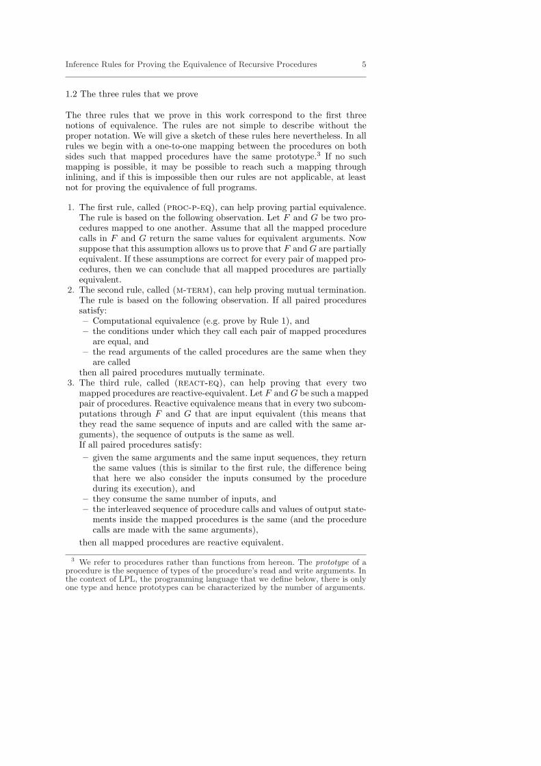
The three rules that we prove in this work correspond to the first threenotions of equivalence. The rules are not simple to describe without theproper notation. We will give a sketch of these rules here nevertheless. In allrules we begin with a one-to-one mapping between the procedures on bothsides such that mapped procedures have the same prototype.3 If no suchmapping is possible, it may be possible to reach such a mapping throughinlining, and if this is impossible then our rules are not applicable, at leastnot for proving the equivalence of full programs.

1. The first rule, called (proc-p-eq), can help proving partial equivalence.The rule is based on the following observation. Let F and G be two pro-cedures mapped to one another. Assume that all the mapped procedurecalls in F and G return the same values for equivalent arguments. Nowsuppose that this assumption allows us to prove that F and G are partiallyequivalent. If these assumptions are correct for every pair of mapped pro-cedures, then we can conclude that all mapped procedures are partiallyequivalent.

2. The second rule, called (m-term), can help proving mutual termination.The rule is based on the following observation. If all paired proceduressatisfy:– Computational equivalence (e.g. prove by Rule 1), and– the conditions under which they call each pair of mapped procedures

are equal, and– the read arguments of the called procedures are the same when they

are calledthen all paired procedures mutually terminate.

3. The third rule, called (react-eq), can help proving that every twomapped procedures are reactive-equivalent. Let F and G be such a mappedpair of procedures. Reactive equivalence means that in every two subcom-putations through F and G that are input equivalent (this means thatthey read the same sequence of inputs and are called with the same ar-guments), the sequence of outputs is the same as well.If all paired procedures satisfy:– given the same arguments and the same input sequences, they return

the same values (this is similar to the first rule, the difference beingthat here we also consider the inputs consumed by the procedureduring its execution), and

– they consume the same number of inputs, and– the interleaved sequence of procedure calls and values of output state-

ments inside the mapped procedures is the same (and the procedurecalls are made with the same arguments),

then all mapped procedures are reactive equivalent.

3 We refer to procedures rather than functions from hereon. The prototype of aprocedure is the sequence of types of the procedure’s read and write arguments. Inthe context of LPL, the programming language that we define below, there is onlyone type and hence prototypes can be characterized by the number of arguments.


Checking all three rules can be automated.The description of the rules and their proof of soundness refer to a simple

programming language called Linear Procedure Language (LPL), which wedefine in Section 2.1, together with its operational semantics. In Sections 3,4 and 5 we state the three inference rules respectively and prove their sound-ness. Each rule is accompanied with an example.

2 Preliminaries

Notation of sequences. An n-long sequence is denoted by 〈l0, . . . , ln−1〉 orby 〈li〉i∈{0,...,n−1}. If the sequence is infinite we write 〈li〉i∈{0,...}. Given twosequences a = 〈ai〉i∈{0,...,n−1} and b = 〈bi〉i∈{0,...,m−1},

a · bis their concatenation of length n + m.

We overload the equality sign (=) to denote sequence equivalence. Giventwo finite sequences a and b

(a = b) ⇔ (|a| = |b| ∧ ∀i ∈ {0, . . . , |a| − 1}. ai = bi) ,

where |a| and |b| denote the number of elements in a and b, respectively.If both a and b are infinite then

(a = b) ⇔ (∀i ≥ 0. ai = bi) ,

and if exactly one of {a, b} is infinite then a 6= b.

Parentheses and brackets We use a convention by which arguments of a func-tion are enclosed in parenthesis, as in f(e), when the function maps valueswithin a single domain. If it maps values between different domains we usebrackets, as in f [e]. References to vector elements, for example, belong to thesecond group, as they map between indices and values in the domain of thevector. Angled brackets (〈·〉) are used for both sequences as shown above,and for tuples.

2.1 The programming language

To define the programming language we assume a set of procedure namesProc= {p0, . . . , pm}, where p0 has a special role as the root procedure (theequivalent of ‘main’ in C). Let D be a domain that contains the constantstrue and false, and no subtypes. Let OD be a set of operations (functionsand predicates) over D. We define a set of variables over this domain: V =⋃

p∈Proc Vp, where Vp is the set of variables of a procedure p. The sets Vp,p ∈ Proc are pairwise disjoint. For expression e over D and V we denote byvars[e] the set of variables that appear in e.

The LPL language is modeled after PLW [6], but is different in variousaspects. For example, it does not contain loops and allows only procedurecalls by value-return.


Definition 1 (Linear Procedure Language (LPL)) The linear proce-dure language (LPL) is defined by the following grammar (lexical elementsof LPL are in bold, and S denotes Statement constructs):

Program :: 〈procedure p(val arg-rp; ret arg-wp):Sp〉p∈Proc

S :: x := e | S;S | if B then S else S fi | if B then S fi |call p(e; x) | return

where p ∈ Proc, e is an expression over OD, and B is a predicate over OD.arg-rp, arg-wp are vectors of Vp variables called, respectively, read formalarguments and write formal arguments, and are used in the body Sp of theprocedure named p. In a procedure call “call p(e; x)”, the expressions e arecalled the actual input arguments and x are called the actual output variables.The following constraints are assumed:

1. The only variables that can appear in the procedure body Sp are from Vp.2. For each procedure call “call p(e, x)” the lengths of e and x are equal to

the lengths of arg-rp and arg-wp, respectively.3. return must appear at the end of any procedure body Sp (p ∈ Proc).

¦

For simplicity LPL is defined so it does not permit global variables anditerative expressions like while loops. Both of these syntactic restrictions donot constrain the expressive power of the language: global variables can bepassed as part of the list of arguments of each procedure, and loops can berewritten as recursive expressions.

Definition 2 (An LPL augmented by location labels) An LPL pro-gram augmented with location labels is derived from an LPL program Pby adding unique labels before[S] and after[S] for each statement S, rightbefore and right after S, respectively. As an exception, for two composedstatements S1 and S2 (i.e., S1; S2), we do not dedicate a label for after[S1];rather, we define after[S1] = before[S2]. ¦

Example 2 Consider the LPL program P at the left of Fig. 2, defined over thedomain Z ∪ {true, false} for which, among others, the operations +,−, =are well-defined. The same program augmented with location labels appearson the right of the same figure.

ut

The partial order ≺ of the locations is any order which satisfies :

1. For any statement S, before[S] ≺ after[S].2. For an if statement S : if B then S1 else S2 fi,

before[S] ≺ before[S1], before[S] ≺ before[S2], after[S1] ≺ after[S] andafter[S2] ≺ after[S].

We denote the set of location labels in the body of procedure p ∈ Procby PCp. Together the set of all location labels is PC

.=⋃

p∈Proc PCp.


procedure p1(val x; ret y):z := x + 1;y := x – 1;return

procedure p0(val w; ret w):if (w = 0) then

w := 1else w := 2fi;call p1(w;w);return

procedure p1(val x; ret y):l1 z := x + 1;l2 y := x – 1;l3 return l4

procedure p0(val w; ret w):l5 if (w = 0) then

l6 w := 1 l7else l8 w := 2 l9

fi;l10 call p1(w;w); l11return l12

Fig. 2 An LPL program (left) and its augmented version (right).

2.2 Operational semantics

A computation of a program P in LPL is a sequence of configurations. Eachconfiguration C = 〈d, O, pc, σ〉 contains the following elements:

1. The natural number d is the depth of the stack at this configuration.2. The function O : {0, . . . , d} 7→ Proc is the order of procedures in the stack

at this configuration.3. pc = 〈pc0, pc1 . . . , pcd〉 is a vector of program location labels4 such that

pc0 ∈ PC0 and for each call level i ∈ {1, . . . , d} pci ∈ PCO[i] (i.e., pci

“points” into the procedure body that is at the ith place in the stack).4. The function σ : {0, . . . , d}×V 7→ D∪{nil} is a valuation of the variables

V of program P at this configuration. The value of variables which arenot active at the i-th call level is invalid i.e., for i ∈ {0, . . . , d}, if O[i] = pand v ∈ V \Vp then σ[〈i, v〉] = nil where nil 6∈ D denotes an invalid value.

A valuation is implicitly defined over a configuration. For an expressione over D and V , we define the value of e in σ in the natural way, i.e., eachvariable evaluates according to the procedure and the stack depth defined bythe configuration. More formally, for a configuration C = 〈d,O, pc, σ〉 and avariable x:

σ[x] .={

σ[〈d, x〉] if x ∈ Vp and p = O[d]nil otherwise

This definition extends naturally to a vector of expressions.When referring to a specific configuration C, we denote its elements

d,O, pc, σ with C.d, C.O, C.pc, C.σ[x] respectively.For a valuation σ, expression e over D and V , levels i, j ∈ {0, . . . , d}, and

a variable x, we denote by σ[〈i, e〉|〈j, x〉] a valuation identical to σ other thanthe valuation of x at level j, which is replaced with the valuation of e at leveli. When the respective levels are clear from the context, we may omit themfrom the notation.

Finally, we denote by σ|i a valuation σ restricted to level i, i.e., σ|i[v] .=σ[〈i, v〉] (v ∈ V ).

4 pc can be thought of as a stack of program counters, hence the notation.


For a configuration C = 〈d,O, pc, σ〉 we denote by current-label[C] theprogram location label at the procedure that is topmost on the stack, i.e.,current-label[C] .= pcd.

Definition 3 (Initial and Terminal configurations in LPL) A config-uration C = 〈d,O, pc, σ〉 with current-label[C] = before[Sp0 ] is called theinitial configuration and must satisfy d = 0 and O[0] = p0. A configurationwith current-label[C] = after[Sp0 ] is called the terminal configuration. ¦Definition 4 (Transition relation in LPL) Let ‘→’ be the least relationamong configurations which satisfies: if C → C ′, C = 〈d,O, pc, σ〉, C ′ =〈d′, O′, pc′, σ′〉 then:

1. If current-label[C] = before[S] for some assign construct S = “x := e”then d′ = d, O′ = O, pc′ = 〈pci〉i∈{0,...,d−1} · 〈after[S]〉, σ′ = σ[e|x].

2. If current-label[C] = before[S] for some construct

S = “if B then S1 else S2 fi”

thend′ = d, O′ = O, pc′ = 〈pci〉i∈{0,...,d−1} · 〈labB〉, σ′ = σ

where

labB ={

before[S1] if σ[B] = truebefore[S2] if σ[B] = false

3. If current-label[C] = after[S1] or current-label[C] = after[S2] for someconstruct

S = “if B then S1 else S2 fi”then

d′ = d, O′ = O, pc′ = 〈pci〉i∈{0,...,d−1} · 〈after[S]〉, σ′ = σ

4. If current-label[C] = before[S] for some call construct S = “call p(e;x)”then d′ = d + 1, O′ = O · 〈p〉, pc′ = 〈pci〉i∈{0,...,d−1} · 〈after[S]〉 ·〈before[Sp]〉, σ′ = σ[〈d, e1〉|〈d+1, (arg-rp)1〉] . . . [〈d, el〉|〈d+1, (arg-rp)l〉]where arg-rp is the vector of formal read variables of procedure p and lis its length.

5. If current-label[C] = before[S] for some return construct S = “return”and d > 0 then d′ = d− 1, O′ = 〈Oi〉i∈{1,...,d−1}, pc′ = 〈pci〉i∈{0,...,d−1},σ′ = σ[〈d, (arg-wp)1〉|〈d−1, x1〉] . . . [〈d, (arg-wp)l〉|〈d−1, xl〉] where arg-wp

is the vector of formal write variables of procedure p, l is its length, and xare the actual output variables of the call statement immediately beforepcd−1.

6. If current-label[C] = before[S] for some return construct S = “return”and d = 0 then d′ = 0, O′ = 〈p0〉, pc′ = 〈after[Sp0 ]〉 and σ′ = σ.

¦Note that the case of current-label[C] = before[S] for a construct S = S1;S2

is always covered by one of the cases in the above definition.Another thing to note is that all write arguments are copied to the actual

variables following a return statement. This solves possible problems thatmay occur if the same variable appears twice in the list of write arguments.


2.3 Computations and subcomputations of LPL programs

A computation of a program P in LPL is a sequence of configurations C =〈C0, C1, . . .〉 such that C0 is an initial configuration and for each i ≤ |C| − 1we have Ci → Ci+1. If the computation is finite then the last configurationmust be terminal.

The proofs throughout this article will be based on the notion of sub-computations. We distinguish between several types of subcomputations, asfollows (an example will be given after the definitions):

Definition 5 (Subcomputation at a level) A continuous subsequence ofa computation is a subcomputation at level d if all its configurations have thesame stack depth d. ¦Clearly every subcomputation at a level is finite.

Definition 6 (Maximal subcomputation at a level) A maximal sub-computation at level d is a subcomputation at level d, such that the successorof its last configuration has stack-depth different than d, or d = 0 and itslast configuration is equal to after[S0]. ¦Definition 7 (Subcomputation from a level) A continuous subsequenceof a computation is a subcomputation from level d if its first configuration C0

has stack depth d, current-label[C0] = before[Sp] for some procedure p andall its configurations have a stack depth of at least d. ¦Definition 8 (Maximal subcomputation from a level) A maximalsubcomputation from level d is a subcomputation from level d which is either

– infinite, or– finite, and,

– if d > 0 the successor of its last configuration has stack-depth smallerthan d, and

– if d = 0, then its last configuration is equal to after[S0].

¦A finite maximal subcomputation is also called closed.

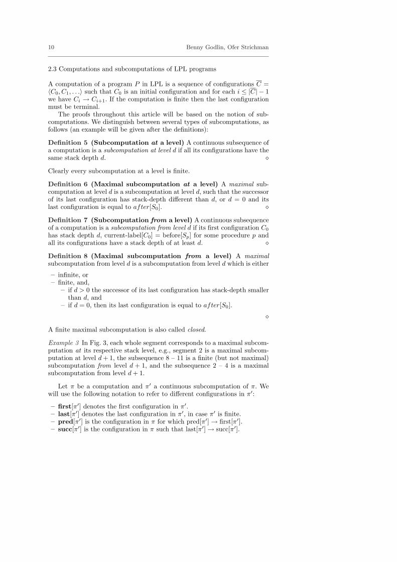
Example 3 In Fig. 3, each whole segment corresponds to a maximal subcom-putation at its respective stack level, e.g., segment 2 is a maximal subcom-putation at level d + 1, the subsequence 8 – 11 is a finite (but not maximal)subcomputation from level d + 1, and the subsequence 2 – 4 is a maximalsubcomputation from level d + 1.

Let π be a computation and π′ a continuous subcomputation of π. Wewill use the following notation to refer to different configurations in π′:

– first[π′] denotes the first configuration in π′.– last[π′] denotes the last configuration in π′, in case π′ is finite.– pred[π′] is the configuration in π for which pred[π′] → first[π′].– succ[π′] is the configuration in π such that last[π′] → succ[π′].


p

1

2

3

4

5

6

7

8

9 11

12

10

d

d + 3

d + 1

d + 2

Fig. 3 A computation through various stack levels. Each rise corresponds to aprocedure call, and each fall to a return statement.

2.4 An assumption about the programs we compare

Two procedures

procedure F (val arg-rF ; ret arg-wF ),procedure G(val arg-rG; ret arg-wG)

are said to have an equivalent prototype if |arg-rF | = |arg-rG| and |arg-wF | =|arg-wG|.

We will assume that the two LPL programs P1 and P2 that we comparehave the following property: |Proc[P1]| = |Proc[P2]|, and there is a 1-1 andonto mapping map : Proc[P1] 7→ Proc[P2] such that if 〈F, G〉 ∈ map then Fand G have an equivalent prototype.

Programs that we wish to prove equivalent and do not fulfill this re-quirement, can sometimes be brought to this state by applying inlining ofprocedures that can not be mapped.

3 A proof rule for partial procedure equivalence

Given the operational semantics of LPL, we now proceed to define a proofrule for the partial equivalence of two LPL procedures. The rule refers tofinite computations only. We delay the discussion on more general cases toSections 4 and 5.

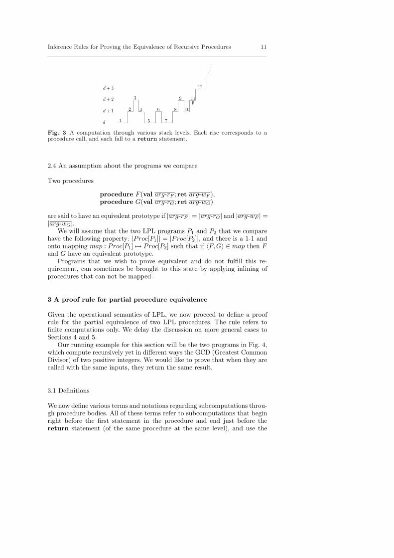
Our running example for this section will be the two programs in Fig. 4,which compute recursively yet in different ways the GCD (Greatest CommonDivisor) of two positive integers. We would like to prove that when they arecalled with the same inputs, they return the same result.

3.1 Definitions

We now define various terms and notations regarding subcomputations throu-gh procedure bodies. All of these terms refer to subcomputations that beginright before the first statement in the procedure and end just before thereturn statement (of the same procedure at the same level), and use the


procedure gcd1(val a,b; ret g):if b = 0 then

g := aelse

a := a mod b;l1 call gcd1(b, a; g) l3

fi;return

procedure gcd2(val x,y; ret z):z := x;if y > 0 then

l2 call gcd2(y, z mod y; z) l4fi;return

Fig. 4 Two procedures to calculate GCD of two positive integers. For better read-ability we only show the labels that we later refer to.

formal arguments of the procedure. We will overload these terms, however,when referring to subcomputations that begin right before the call statementto the same procedure and end right after it, and consequently use the ac-tual arguments of the procedure. This overloading will repeat itself in futuresections as well.

Definition 9 (Argument-equivalence of subcomputations with re-spect to procedures) Given two procedures F ∈ Proc[P1] and G ∈Proc[P2] such that 〈F, G〉 ∈ map, for any two computations π1 in P1 andπ2 in P2, π′1 and π′2 are argument-equivalent with respect to F and G if thefollowing holds:

1. π′1 and π′2 are maximal subcomputations of π1 and π2 from some levelsd1 and d2 respectively,

2. current-label[first[π′1]] = before[F ] and current-label[first[π′2]] = before[G],and

3. first[π′1].σ[arg-rF ] = first[π′2].σ[arg-rG],

¦

Definition 10 (Partial computational equivalence of procedures) Iffor every argument-equivalent finite subcomputations π′1 and π′2 (these areclosed by definition) with respect to two procedures F and G,

last[π′1].σ[arg-wF ] = last[π′2].σ[arg-wG]

then F and G are partially computationally equivalent. ¦

Denote by comp-equiv(F, G) the fact that F and G are partially computa-tionally equivalent. The computational equivalence is only partial because itdoes not consider infinite computations. From hereon when we talk aboutcomputational equivalence we mean partial computational equivalence.

Our proof rule uses uninterpreted procedures, which are useful for reason-ing about an abstract system. The only information that the decision pro-cedure has about them is that they are consistent, i.e., that given the sameinputs, they produce the same outputs. We still need a semantics for suchprocedures, in order to be able to define subcomputations that go throughthem. In terms of the semantics, then, an uninterpreted procedure U is thesame as an empty procedure in LPL (a procedure with a single statement –


(3.1) ∀〈F, G〉 ∈ map. {(3.2) `LUP comp-equiv(F UP , GUP ) }

(3.3) ∀〈F, G〉 ∈ map. comp-equiv(F, G)(proc-p-eq) (3)

Fig. 5 Rule (proc-p-eq): An inference rule for proving the partial equivalence ofprocedures.

return), other than the fact that it preserves the congruence condition:For every two subcomputations π1 and π2 through U ,

first[π1].σ[arg-rU ] = first[π2].σ[arg-rU ]→last[π1].σ[arg-wU ] = last[π2].σ[arg-wU ] .

(1)

There are well known decision procedures for reasoning about formulasthat involve uninterpreted functions – see, for example, Shostak’s algorithm[14], and accordingly most theorem provers support them. Such algorithmscan be easily adapted to handle procedures rather than functions.

3.2 Rule (proc-p-eq)

Defining the proof rule requires one more definition.Let UP be a mapping of the procedures in Proc[P1]∪Proc[P2] to respec-

tive uninterpreted procedures, such that:

〈F,G〉 ∈ map ⇐⇒ UP(F ) = UP(G) , (2)

and such that each procedure is mapped to an uninterpreted procedure withan equivalent prototype.

Definition 11 (Isolated procedure) The isolated version of a procedureF , denoted FUP , is derived from F by replacing all of its procedure callsby calls to the corresponding uninterpreted procedures, i.e., FUP .= F [f ←UP(f)|f ∈ Proc[P ]]. ¦For example, Fig. 6 presents an isolated version of the programs in Fig. 4.

Rule (proc-p-eq), appearing in Fig. 5, is based on the following obser-vation. Let F and G be two procedures such that 〈F,G〉 ∈ map. If assumingthat all the mapped procedure calls in F and G return the same values forequivalent arguments enables us to prove that F and G are equivalent, thenwe can conclude that F and G are equivalent.

The rule assumes a proof system LUP. LUP is any sound proof system fora restricted version of the programming language in which there are no callsto interpreted procedures, and hence, in particular, no recursion5, and it can

5 In LPL there are no loops, but in case (proc-p-eq) is applied to other lan-guages, LUP is required to handle a restricted version of the language with no pro-cedure calls, recursion or loops. Indeed, under this restriction there are sound andcomplete decision procedures for deciding the validity of assertions over popularprogramming languages such as C, as was mentioned in the introduction.


procedure gcd1(val a,b; ret g):if b = 0 then

g := aelse

a := a mod b;call H(b, a; g)

fi;return

procedure gcd2(val x,y; ret z):z := x;if y > 0 then

call H(y, z mod y; z)

fi;return

Fig. 6 After isolation of the procedures, i.e., replacing their procedure calls withcalls to the uninterpreted procedure H.

reason about uninterpreted procedures. LUP is not required to be complete,because (proc-p-eq) is incomplete in any case. Nevertheless, completenessis desirable since it makes the rule more useful.

Example 4 Following are two instantiations of rule (proc-p-eq).

– The two programs contain one recursive procedure each, called f and gsuch that map = {〈f, g〉}.

`LUP comp-equiv(f [f ← UP(f)], g[g ← UP(g)])comp-equiv(f, g)

Recall that f [f ← UP(f)] means that the call to f inside f is replacedwith a call to UP(f) (isolation).

– The two compared programs contain two mutually recursive procedureseach, f1, f2 and g1, g2 respectively, such that map = {〈f1, g1〉, 〈f2, g2〉},and f1 calls f2, f2 calls f1, g1 calls g2 and g2 calls g1.

`LUP comp-equiv(f1[f2 ← UP(f2)], g1[g2 ← UP(g2)]),`LUP comp-equiv(f2[f1 ← UP(f1)], g2[g1 ← UP(g1)])

comp-equiv(f1, g1), comp-equiv(f2, g2) utExample 5 Consider once again the two programs in Fig. 4. There is onlyone procedure in each program, which we naturally map to one another.Let H be the uninterpreted procedure to which we map gcd1 and gcd2, i.e.,H = UP(gcd1) = UP(gcd2). Figure 6 presents the isolated programs.

To prove the computational equivalence of the two procedures, we needto first translate them to formulas expressing their respective transition rela-tions. A convenient way to do so is to use Static Single Assignment (SSA) [3].Briefly, this means that in each assignment of the form x = exp; the left-hand side variable x is replaced with a new variable, say x1. Any referenceto x after this line and before x is potentially assigned again, is replacedwith the new variable x1 (recall that this is done in a context of a programwithout loops). In addition, assignments are guarded according to the controlflow. After this transformation, the statements are conjoined: the resultingequation represents the states of the original program. If a subcomputationthrough a procedure is valid then it can be associated with an assignmentthat satisfies the SSA form of this procedure.


The SSA form of gcd1 is

Tgcd1 =

a0 = a ∧b0 = b ∧b0 = 0 → g0 = a0 ∧(b0 6= 0 → a1 = (a0 mod b0)) ∧ (b0 = 0 → a1 = a0) ∧(b0 6= 0 → H(b0, a1; g1)) ∧ (b0 = 0 → g1 = g0) ∧g = g1

. (4)

The SSA form of gcd2 is

Tgcd2 =

x0 = x ∧y0 = y ∧z0 = x0 ∧(y0 > 0 → H(y0, (z0 mod y0); z1)) ∧ (y0 ≤ 0 → z1 = z0) ∧z = z1

.

(5)The premise of rule (proc-p-eq) requires proving computational equivalence(see Definition 10), which in this case amounts to proving the validity of thefollowing formula over positive integers:

(a = x ∧ b = y ∧ Tgcd1 ∧ Tgcd2) → g = z . (6)

Many theorem provers can prove such formulas fully automatically, and henceestablish the partial computational equivalence of gcd1 and gcd2. ut

It is important to note that while the premise refers to procedures thatare isolated from other procedures, the consequent refers to the original pro-cedures. Hence, while LUP is required to reason about executions of boundedlength (the length of one procedure body) the consequent refers to unboundedexecutions.

To conclude this section, let us mention that rule (proc-p-eq) is inspiredby Hoare’s rule for recursive procedures:

{p}call proc{q} `H {p}S{q}{p}call proc{q} (REC)

(where S is the body of procedure proc). Indeed, both in this rule and in rule(proc-p-eq), the premise requires to prove that the body of the procedurewithout its recursive calls satisfies the pre-post condition relation that wewish to establish, assuming the recursive calls already do so.

3.3 Rule (proc-p-eq) is sound

Let π be a computation of some program P1. Each subcomputation π′ fromlevel d consists of a set of maximal subcomputations at level d, which aredenoted by in(π′, d), and a set of maximal subcomputations from level d+1,which are denoted by from(π′, d + 1). The members of these two sets of


d p1

p2

p2

p4

1

5 7

9

2

3

4 8

1,9

5,7

6

3

2,4,8

d+3

d+2

d+1

p4

p26

p0

p1

p2

Fig. 7 (left) A computation and its stack levels. The numbering on the horizontalsegments are for reference only. (right) The stack-level tree corresponding to thecomputation on the left.

computations alternate in π′. For example, in the left drawing in Fig. 7,segments 2,4,8 are separate subcomputations at level d + 1, and segments 3,and 5–7 are subcomputations from level d + 2.

Definition 12 (Stack-level tree) A stack-level tree of a maximal subcom-putation π from some level, is a tree in which each node at height d (d > 0)represents the set of subcomputations at level d from the time the computa-tion entered level d until it returned to its calling procedure at level d − 1.Node n′ is a child of a node n if and only if it contains one subcomputationthat is a continuation (in π) of a subcomputation in n. ¦

Note that the root of a stack-level tree is the node that contains first[π]in one of its subcomputations. The leafs are closed subcomputations fromsome level which return without executing a procedure call. Also note thatthe subcomputations in a node at level d are all part of the same closedsubcomputation π′ from level d (this is exactly the set in(π′, d)).

The stack-level tree depth is the maximal length of a path from its rootto some leaf. This is also the maximal difference between the depth of thelevel of any of its leafs and the level of its root. If the stack-level tree is notfinite then its depth is undefined.

Denote by d[n] the level of node n and by p[n] the procedure associatedwith this node.

Example 6 Figure 7 demonstrates a subcomputation π from level d (left)and its corresponding stack-level tree (upside down, in order to emphasize itscorrespondence to the computation). The set in(π, d) = {1, 9} is representedby the root. Each rise in the stack level is associated with a procedure call(in this case, calls to p1,p2,p4,p2), and each fall with a return statement.To the left of each node n in the tree, appears the procedure p[n] (here weassumed that the computation entered level d due to a call to a procedurep0). The depth of this stack-level tree is 4.

utTheorem 1 (Soundness) If the proof system LUP is sound then the rule(proc-p-eq) is sound.

Proof By induction on the depth d of the stack-level tree. Since we consideronly finite computations, the stack-level trees are finite and their depthsare well defined. Let P1 and P2 be two programs in LPL, π1 and π2 closedsubcomputations from some levels in P1 and P2 respectively, t1 and t2 the


stack-level trees of these computations, n1 and n2 the root nodes of t1 and t2respectively. Also, let F = p[n1] and G = p[n2] where 〈F,G〉 ∈ map. Assumealso that π1 and π2 are argument-equivalent with respect to F and G.

Base: If both n1 and n2 are leafs in t1 and t2 then the conclusion is provenby the premise of the rule without using the uninterpreted procedures. Asπ1 and π2 contain no calls to procedures, then they are also valid compu-tations through FUP and GUP , respectively. Therefore, by the soundness ofthe proof system LUP, π1 and π2 must satisfy comp-equiv(FUP , GUP ) whichentails the equality of arg-w values at their ends. Therefore, π1 and π2 satisfythe condition in comp-equiv(F,G).

Step: Assume the consequent (3.3) is true for all stack-level trees of depthat most i. We prove the consequent for computations with stack-level treest1 and t2 such that at least one of them is of depth i + 1.

1. Consider the computation π1. We construct a computation π′1 in FUP ,which is the same as π1 in the level of n1, with the following change. Eachsubcomputation of π1 in a deeper level caused by a call cF , is replaced bya subcomputation through an uninterpreted procedure UP(callee[cF ]),which returns the same value as returned by cF (where callee[cF ] is theprocedure called in the call statement cF ). In a similar way we constructa computation π′2 in GUP corresponding to π2.

The notations we use in this proof correspond to Fig. 8. Specifically,

A1 = first[π1], A′1 = first[π′1], A′2 = first[π′2], A2 = first[π2],B1 = last[π1], B′

1 = last[π′1], B′2 = last[π′2], B2 = last[π2] .

2. As π1 and π2 are argument-equivalent we have

A1.σ[arg-rF ] = A2.σ[arg-rG] .

By definition,A′1.σ[arg-rF ] = A1.σ[arg-rF ]

andA′2.σ[arg-rG] = A2.σ[arg-rG] .

By transitivity of equality A′1.σ[arg-rF ] = A′2.σ[arg-rG].

3. We now prove that the subcomputations π′1 and π′2 are valid computationsthrough FUP and GUP . As π′1 and π′2 differ from π1 and π2 only bysubcomputations through uninterpreted procedures (that replace calls toother procedures), we need to check that they satisfy the congruencecondition, as stated in (1). Other parts of π′1 and π′2 are valid becauseπ1 and π2 are valid subcomputations. Consider any pair of calls c1 and


A′1 B′

1

π′1

A2 B2

π2

A′2 B′

2

π′2

A1 B1

π1

arg-r arg-w

Fig. 8 A diagram for the proof of Theorem 1. Dotted lines indicate an equivalence(either that we assume as a premise or that we need to prove) in the argumentthat labels the line. We do not write all labels to avoid congestion – see moredetails in the proof. π1 is a subcomputation through F . π′1 is the the correspondingsubcomputation through F UP , the isolated version of F . The same applies to π2

and π′2 with respect to G. The induction step shows that if the read arguments arethe same in A.1 and A.2, then the write arguments have equal values in B.1 andB.2.

c2 in π1 and π2 from the current levels d[n1] and d[n2] to procedures p1

and p2 respectively, such that 〈p1, p2〉 ∈ map. Let c′1 and c′2 be the callsto UP(p1) and UP(p2) which replace c1 and c2 in π′1 and π′2. Note thatUP(p1) = UP(p2) since 〈p1, p2〉 ∈ map.By the induction hypothesis, procedures p1, p2 satisfy comp-equiv(p1, p2)for all subcomputations of depth ≤ i, and in particular for subcomputa-tions of π1, π2 that begin in c1 and c2. By construction, the input andoutput values of c1 are equal to those of c′1. Similarly, the input and outputvalues of c2 are equal to those of c′2. Consequently, the pair of calls c′1 andc′2 to the uninterpreted procedure UP(p1) satisfy the congruence condi-tion. Hence, π′1 and π′2 are legal subcomputations through FUP and GUP .

4. By the rule premise, any two computations through FUP and GUP sat-isfy comp-equiv(FUP , GUP ). Particularly, as π′1 and π′2 are argument-equivalent by step 2, this entails that B′

1.σ[arg-wF ] = B′2.σ[arg-wG].

By construction, B1.σ[arg-wF ] = B′1.σ[arg-wF ] and B2.σ[arg-wG] =

B′2.σ[arg-wG]. Therefore, by transitivity,

B1.σ[arg-wF ] = B2.σ[arg-wG] ,

which proves that π1 and π2 satisfy comp-equiv(F, G).

ut

4 A proof rule for mutual termination of procedures

Rule (proc-p-eq) only proves partial equivalence, because it only refers tofinite computations. It is desirable, in the context of equivalence checking, to


(7.1) ∀〈F, G〉 ∈ map. {(7.2) comp-equiv(F, G) ∧(7.3) `LUP reach-equiv(F UP , GUP ) }

(7.4) ∀〈F, G〉 ∈ map. mutual-terminate(F, G)(m-term) (7)

Fig. 9 Rule (m-term): An inference rule for proving the mutual termination ofprocedures. Note that Premise 7.2 can be proven by the (proc-p-eq) rule.

prove that the two procedures mutually terminate. If, in addition, termina-tion of one of the programs is proven, then ‘total equivalence’ is established.

4.1 Definitions

Definition 13 (Mutual termination of procedures) If for every pair ofargument-equivalent subcomputations π′1 and π′2 with respect to two proce-dures F and G, it holds that π′1 is finite if and only if π′2 is finite, then F andG are mutually terminating. ¦Denote by mutual-terminate(F, G) the fact that F and G are mutually ter-minating.

Definition 14 (Reach equivalence of procedures) Procedures F andG are reach-equivalent if for every pair of argument-equivalent subcompu-tation π and τ through F and G respectively, for every call statementcF = “call p1” in F (in G), there exists a call cG = “call p2” in G (inF ) such that 〈p1, p2〉 ∈ map, and π and τ reach cF and cG respectively withthe same read arguments, or do not reach them at all.

Denote by reach-equiv(F, G) the fact that F and G are reach-equivalent.Note that checking for reach-equivalence amounts to proving the equiva-lence of the ‘guards’ leading to each of the mapped procedure calls (i.e., theconjunction of conditions that need to be satisfied in order to reach theseprogram locations), and the equivalence of the arguments before the calls.This will be demonstrated in two examples later on.

4.2 Rule (m-term)

The mutual termination rule (m-term) is stated in Fig. 9. It is interestingto note that unlike proofs of procedure termination, here we do not rely onwell-founded sets (see, for example, [6,?]).

Example 7 Continuing Example 5, we now prove the mutual termination ofthe two programs in Fig. 4. Since we already proved comp-equiv(gcd1, gcd2)in Example 5, it is left to check Premise (7.3), i.e.,

`LUP reach-equiv(gcd1UP , gcd2

UP ) .


Since in this case we only have a single procedure call in each side, the onlything we need to check in order to establish reach-equivalence, is that theguards controlling their calls are equivalent, and that they are called withthe same input arguments. The verification condition is thus:

(Tgcd1 ∧ Tgcd2 ∧ (a = x) ∧ (b = y)) →( ((y0 > 0) ↔ (b0 6= 0)) ∧ //Equal guards

((y0 > 0) → ((b0 = y0) ∧ (a1 = z0 mod y0))) ) //Equal inputs(8)

where Tgcd1 and Tgcd2 are as defined in Eq. (4) and (5).ut

4.3 Rule (m-term) is sound

We now prove the following:

Theorem 2 (Soundness) If the proof system LUP is sound then the rule(m-term) is sound.

Proof In case the computations of P1 and P2 are both finite or both infinitethe consequent of the rule holds by definition. It is left to consider the casein which one of the computations is finite and the other is infinite. We showthat if the premise of (m-term) holds such a case is impossible.

Let P1 and P2 be two programs in LPL, π1 and π2 maximal subcompu-tations from some levels in P1 and P2 respectively, t1 and t2 the stack-leveltrees of these computations, n1 and n2 the root nodes of t1 and t2 respectivelyand F = p[n1] and G = p[n2]. Assume π1 and π2 are argument-equivalent.Without loss of generality assume also that π1 is finite and π2 is not.

Consider the computation π1. We continue as in the proof of Theorem 1.We construct a computation π′1 in FUP , which is the same as π1 in the levelof n1, with the following change. Each closed subcomputation at a deeperlevel caused by a call cF , is replaced with a subcomputation through an un-interpreted procedure UP(callee[cF ]), which receives and returns the samevalues as received and returned by cF . In a similar way we construct a com-putation π′2 in GUP corresponding to π2. By Premise (7.2), any pair of callsto some procedures p1 and p2 (related by map) satisfy comp-equiv(p1, p2).Thus, any pair of calls to an uninterpreted procedure UP(p1) (which is equalto UP(p2)) in π′1 and π′2 satisfy the congruence condition (see (1)). As inthe proof of the (proc-p-eq) rule, this is sufficient to conclude that π′1 andπ′2 are valid subcomputations through FUP and GUP (but not necessarilyclosed).

By Premise (7.3) of the rule and the soundness of the underlying proofsystem LUP, π′1 and π′2 satisfy the condition in reach-equiv(FUP , GUP ) . Itis left to show that this implies that π2 must be finite. We will prove thisfact by induction on the depth d of t1.


Base: d = 0. In this case n1 is a leaf and π1 does not execute any callstatements. Assume that π2 executes some call statement cG in G. Sinceby Premise (7.3) reach-equiv(FUP , GUP ) holds, then there must be somecall cF in F such that 〈callee[cF ], callee[cG]〉 ∈ map and some configurationC1 ∈ π′1 such that current-label[C1] = before[cF ] (i.e., π′1 reaches the cF call).But this is impossible as n1 is a leaf. Thus π2 cannot be infinite.

Step:

1. Assume (by the induction hypothesis) that if π1 is a finite computationwith stack-level tree t1 of depth d < i then any π2 such that

first[π1].σ[arg-rF ] = first[π2].σ[arg-rG],

cannot be infinite. We now prove this for π1 with t1 of depth d = i.

2. Let π̂2 be some subcomputation of π2 from level d[n2] + 1, C2 be theconfiguration in π2 which comes immediately before π̂2 (C2 = pred[π̂2]).Let cG be the call statement in G which is executed at C2 (in other wordscurrent-label[C2] = before[cG]).

3. Since by Premise (7.3) reach-equiv(FUP , GUP ), there must be some callcF in F such that 〈callee[cF ], callee[cG]〉 ∈ map and some configurationC1 ∈ π′1 from which the call cF is executed (i.e., current-label[C1] =before[cF ]), and C1 passes the same input argument values to cF as C2

to cG. In other words, if cF = call p1(e1;x1) and cG = call p2(e2; x2),then C1.σ[e1] = C2.σ[e2]. But then, there is a subcomputation π̂1 of π1

from level d[n1] + 1 which starts immediately after C1 (C1 = pred[π̂1]]).

4. π̂1 is finite because π1 is finite. The stack-level tree t̂1 of π̂1 is a subtreeof t1 and its depth is less than i. Therefore, by the induction hypothesis(the assumption in item 1) π̂2 must be finite as well.

5. In this way, all subcomputations of π2 from level d[n2] + 1 are finite. Bydefinition, all subcomputations of π2 at level d[n2] are finite. Thereforeπ2 is finite.

ut

4.4 Using rule (m-term): a long example

In this example we set the domain D to be the set of binary trees with naturalvalues in the leafs and the + and * operators at internal nodes6.

Let t1, t2 ∈ D. We define the following operators:

– isleaf(t1) returns true if t1 is a leaf and false otherwise.

6 To be consistent with the definition of LPL (Definition 1), the domain mustalso include true and false. Hence we also set the constants true and false tobe the leafs with 1 and 0 values respectively.


– isplus(t1) returns true if t1 has ‘+’ in its root node and false otherwise.– leftson(t1) returns false if t1 is a leaf, and the tree which is its left son

otherwise.– doplus(l1, l2) returns a leaf with a value equal to the sum of the values in

l1 and l2, if l1 and l2 are leafs, and false otherwise.

The operators ismult(t1), rightson(t1) and domult(t1, t2) are defined sim-ilarly to isplus, leftson and doplus, respectively.

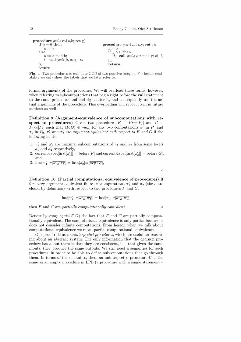
The two procedures in Fig. 10 calculate the value of an expression tree.

procedure Eval1(val a; ret r):if isleaf(a) then

r := aelse

if isplus(a) thenl1 call Plus1(a; r) l3

elseif ismult(a) then

l5 call Mult1(a; r) l7fi

fifireturn

procedure Plus1(val a; ret r):l9 call Eval1(leftson(a); v);l11 call Eval1(rightson(a); u);r := doplus(v, u);return

procedure Mult1(val a; ret r):l13 call Eval1(leftson(a); v);l15 call Eval1(rightson(a); u);r := domult(v, u);return

procedure Eval2(val x; ret y):if isleaf(x) then

y := xelse

if ismult(x) thenl2 call Mult2(x; y) l4

elseif isplus(x) then

l6 call Plus2(x; y) l8fi

fifireturn

procedure Plus2(val x; ret y):l10 call Eval2(rightson(x); w);l12 call Eval2(leftson(x); z);y := doplus(w, z);return

procedure Mult2(val x; ret y):l14 call Eval2(rightson(x); w);l16 call Eval2(leftson(x); z);y := domult(w, z);return

Fig. 10 Two procedures to calculate the value of an expression tree. Only labelsaround the call constructs are shown.

We introduce three uninterpreted procedures E,P and M and set themapping UP to satisfy

UP(Eval1) = UP(Eval2) = E,UP(Plus1) = UP(Plus2) = P,UP(Mult1) = UP(Mult2) = M .


The SSA form of the formulas which represent the possible computationsof isolated procedure bodies are:

TEval1 =

a0 = a ∧(isleaf (a0) → r1 = a0) ∧(¬ isleaf (a0) ∧ isplus(a0) → P (a0, r1)) ∧(¬ isleaf (a0) ∧ ¬ isplus(a0) ∧ ismult(a0) → M(a0, r1)) ∧r = r1

TEval2 =

x0 = x ∧(isleaf (x0) → y1 = x0) ∧(¬ isleaf (x0) ∧ ismult(x0) → M(x0, y1)) ∧(¬ isleaf (x0) ∧ ¬ ismult(x0) ∧ isplus(x0) → P (x0, y1)) ∧y = y1

TPlus1 =

a0 = a ∧E(leftson(a0), v1) ∧E(rightson(a0), u1) ∧r1 = doplus(v1, u1) ∧r = r1

TPlus2 =

x0 = x ∧E(rightson(x0), w1) ∧E(leftson(x0), z1) ∧y1 = doplus(w1, z1) ∧y = y1

TMult1 =

a0 = a ∧E(leftson(a0), v1) ∧E(rightson(a0), u1) ∧r1 = domult(v1, u1) ∧r = r1

TMult2 =

x0 = x ∧E(rightson(x0), w1) ∧E(leftson(x0), z1) ∧y1 = domult(w1, z1) ∧y = y1

Proving partial computational equivalence for each of the procedure pairsamounts to proving the following formulas to be valid:

(a = x ∧ TEval1 ∧ TEval2) → r = y

(a = x ∧ TPlus1 ∧ TPlus2) → r = y

(a = x ∧ TMult1 ∧ TMult2) → r = y .

To prove these formulas it is enough for LUF to know the following factsabout the operators of the domain:

∀l1, l2(doplus(l1, l2) = doplus(l2, l1) ∧ domult(l1, l2) = domult(l2, l1))∀t1(isleaf (t1) → ¬ isplus(t1) ∧ ¬ ismult(t1))∀t1(isplus(t1) → ¬ ismult(t1) ∧ ¬ isleaf (t1))∀t1(ismult(t1) → ¬ isleaf (t1) ∧ ¬ isplus(t1))

This concludes the proof of partial computational equivalence using rule(proc-p-eq). To prove mutual termination using the (m-term) rule we needin addition to verify reach-equivalence of each pair of procedures.

To check reach-equivalence we should check that the guards and the readarguments at labels of related calls are equivalent. This can be expressed bythe following formulas:


ϕ1 = ( g1 = (¬ isleaf (a0) ∧ isplus(a0)) ∧g2 = (¬ isleaf (x0) ∧ ¬ ismult(x0) ∧ isplus(x0)) ∧g3 = (¬ isleaf (a0) ∧ ¬ isplus(a0) ∧ ismult(a0)) ∧g4 = (¬ isleaf (x0) ∧ ismult(x0)) ∧g1 ↔ g2 ∧g3 ↔ g4 ∧g1 → a0 = x0 ∧g3 → a0 = x0)

The guards at all labels in Plus1, P lus2,Mult1 and Mult2 are all true, there-fore the reach-equivalence formulas for these procedures collapse to:

ϕ2 = ϕ3 = ( (leftson(a0) = rightson(x0) ∨ leftson(a0) = leftson(x0)) ∧(rightson(a0) = rightson(x0) ∨ rightson(a0) = leftson(x0)) ∧(leftson(a0) = rightson(x0) ∨ rightson(a0) = rightson(x0)) ∧(leftson(a0) = leftson(x0) ∨ rightson(a0) = leftson(x0)))

In this formula each call in each side is mapped to one of the calls on theother side: the first two lines map calls of side one to calls on side two, andthe last two lines map calls of side two to side one. Finally, the formulas thatneed to be validated are:

(a = x ∧ TEval1 ∧ TEval2) → ϕ1

(a = x ∧ TPlus1 ∧ TPlus2) → ϕ2

(a = x ∧ TMult1 ∧ TMult2) → ϕ3 .

5 A proof rule for equivalence of reactive programs

Rules (proc-p-eq) and (m-term) that we studied in the previous two sec-tions, are concerned with equivalence of finite programs, and with proving themutual termination of programs, respectively. In this section we introducea rule that generalizes (proc-p-eq) in the sense that it is not restricted tofinite computations. This generalization is necessary for reactive programs.We say that two reactive procedures F and G are reactively equivalent ifgiven the same input sequences, their output sequences are the same.

5.1 Definitions

The introduction of the rule and later on the proof requires an extension ofLPL to allow input and output constructs:

Definition 15 (LPL with I/O constructs (LPL+IO)) LPL+IO is theLPL programming language with two additional statement constructs:

input(x) | output(e)

where x ∈ V is a variable and e is an expression over OD. If a sequenceof input constructs appear in a procedure they must appear before any


other statement in that procedure. This fact is important for the proof ofcorrectness.7 ¦

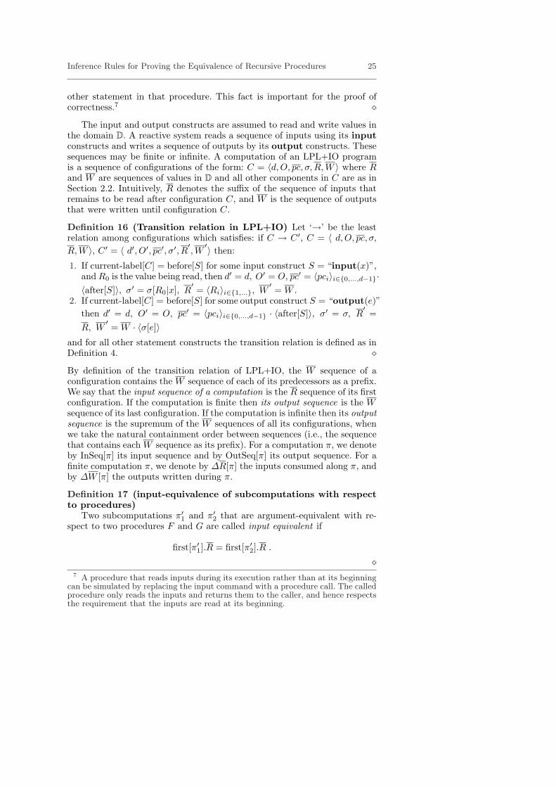
The input and output constructs are assumed to read and write values inthe domain D. A reactive system reads a sequence of inputs using its inputconstructs and writes a sequence of outputs by its output constructs. Thesesequences may be finite or infinite. A computation of an LPL+IO programis a sequence of configurations of the form: C = 〈d,O, pc, σ, R, W 〉 where Rand W are sequences of values in D and all other components in C are as inSection 2.2. Intuitively, R denotes the suffix of the sequence of inputs thatremains to be read after configuration C, and W is the sequence of outputsthat were written until configuration C.

Definition 16 (Transition relation in LPL+IO) Let ‘→’ be the leastrelation among configurations which satisfies: if C → C ′, C = 〈 d,O, pc, σ,

R, W 〉, C ′ = 〈 d′, O′, pc′, σ′, R′, W

′〉 then:

1. If current-label[C] = before[S] for some input construct S = “input(x)”,and R0 is the value being read, then d′ = d, O′ = O, pc′ = 〈pci〉i∈{0,...,d−1}·〈after[S]〉, σ′ = σ[R0|x], R

′= 〈Ri〉i∈{1,...}, W

′= W .

2. If current-label[C] = before[S] for some output construct S = “output(e)”then d′ = d, O′ = O, pc′ = 〈pci〉i∈{0,...,d−1} · 〈after[S]〉, σ′ = σ, R

′=

R, W′= W · 〈σ[e]〉

and for all other statement constructs the transition relation is defined as inDefinition 4. ¦By definition of the transition relation of LPL+IO, the W sequence of aconfiguration contains the W sequence of each of its predecessors as a prefix.We say that the input sequence of a computation is the R sequence of its firstconfiguration. If the computation is finite then its output sequence is the Wsequence of its last configuration. If the computation is infinite then its outputsequence is the supremum of the W sequences of all its configurations, whenwe take the natural containment order between sequences (i.e., the sequencethat contains each W sequence as its prefix). For a computation π, we denoteby InSeq[π] its input sequence and by OutSeq[π] its output sequence. For afinite computation π, we denote by ∆R[π] the inputs consumed along π, andby ∆W [π] the outputs written during π.

Definition 17 (input-equivalence of subcomputations with respectto procedures)

Two subcomputations π′1 and π′2 that are argument-equivalent with re-spect to two procedures F and G are called input equivalent if

first[π′1].R = first[π′2].R .

¦7 A procedure that reads inputs during its execution rather than at its beginning

can be simulated by replacing the input command with a procedure call. The calledprocedure only reads the inputs and returns them to the caller, and hence respectsthe requirement that the inputs are read at its beginning.


(9.1) ∀〈F, G〉 ∈ map. {(9.2) `LUP return-values-equiv(F UP , GUP ) ∧(9.3) `LUP input-suffix -equiv(F UP , GUP ) ∧(9.4) `LUP call-output-seq-equiv(F UP , GUP ) }

(9.5) ∀〈F, G〉 ∈ map. reactive-equiv(F, G)(react-eq) (9)

Fig. 11 Rule (react-eq): An inference rule for proving the reactive equivalenceof procedures.

In other words, two subcomputations are input equivalent with respect toprocedures F and G if they start at the beginnings of F and G respectivelywith equivalent read arguments and equivalent input sequences.

We will use the following notations in this section, for procedures F andG. The formal definitions of these terms appear in Appendix A.

1. reactive-equiv(F,G) – Every two input-equivalent subcomputations withrespect to F and G generate equivalent output sequences until returningfrom F and G, or forever if they do not return.

2. return-values-equiv(F, G) – The last configurations of every two input-equivalent finite subcomputations with respect to F and G that endin the return from F and G, valuate equally the write-arguments of Fand G, respectively. (note that return-values-equiv(F, G) is the same ascomp-equiv(F, G) other than the fact that it requires the subcomputa-tions to be input equivalent and not only argument equivalent).

3. input-suffix -equiv(F, G) – Every two input-equivalent finite subcomputa-tions with respect to F and G that end at the return from F and G, have(at return) the same remaining sequence of inputs.

4. call-output-seq-equiv(F, G) – Every two input-equivalent subcomputa-tions with respect to F and G, generate the same sequence of proce-dure calls and output statements, where corresponding procedure callsare called with equal inputs (read-arguments and input sequences), andoutput statements output equal values.

5.2 Rule (react-eq)

Figure 11 presents rule (react-eq), which can be used for proving equiva-lence of reactive procedures.

5.3 Rule (react-eq) is sound

Theorem 3 (Soundness) If the proof system LUP is sound then rule (react-eq) is sound.


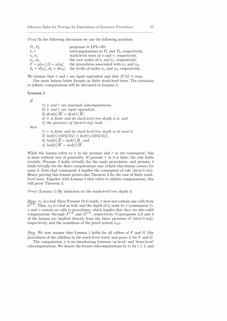
Proof In the following discussion we use the following notation:

P1, P2 programs in LPL+IOπ, τ subcomputations in P1 and P2, respectively,t1, t2 stack-level trees of π and τ , respectively,n1, n2 the root nodes of t1 and t2, respectively,F = p[n1], G = p[n2] the procedures associated with n1 and n2,d1 = d[n1], d2 = d[n2] the levels of nodes n1 and n2, respectively.

We assume that π and τ are input equivalent and that 〈F, G〉 ∈ map.Our main lemma below focuses on finite stack-level trees. The extension

to infinite computations will be discussed in Lemma 5.

Lemma 1

If1) π and τ are maximal subcomputations,2) π and τ are input equivalent,3) first[π].W = first[τ ].W ,4) π is finite and its stack-level tree depth is d, and5) the premises of (react-eq) hold,

then1) τ is finite and its stack-level tree depth is at most d,2) last[π].σ[arg-wF ] = last[τ ].σ[arg-wG],3) last[π].R = last[τ ].R, and4) last[π].W = last[τ ].W .

While the lemma refers to π in the premise and τ in the consequent, thisis done without loss of generality. If premise 1 or 2 is false, the rule holdstrivially. Premise 3 holds trivially for the main procedures, and premise 4holds trivially for the finite computations case (which this lemma covers) forsome d. Note that consequent 4 implies the consequent of rule (react-eq).Hence proving this lemma proves also Theorem 3 for the case of finite stack-level trees. Together with Lemma 5 that refers to infinite computations, thiswill prove Theorem 3.

Proof (Lemma 1) By induction on the stack-level tree depth d.

Base: n1 is a leaf. Since Premise (9.4) holds, τ does not contain any calls fromGUP . Thus, n2 is a leaf as well, and the depth of t2 must be 1 (consequent 1).π and τ contain no calls to procedures, which implies that they are also validcomputations through FUP and GUP , respectively. Consequents 2,3 and 4of the lemma are implied directly from the three premises of (react-eq),respectively, and the soundness of the proof system LUP.

Step: We now assume that Lemma 1 holds for all callees of F and G (theprocedures of the children in the stack-level trees) and prove it for F and G.

The computation π is an interleaving between ‘at-level’ and ‘from-level’subcomputations. We denote the former subcomputations by π̄i for i ≥ 1, and


the latter by π̂j for j ≥ 1. For example, the subcomputation correspondingto level d+1 in the left drawing of Fig. 7 has three ‘at-level’ segments that wenumber π̄1, π̄2, π̄3 (corresponding to segments 2,4,8 in the drawing) and two‘from-level’ subcomputations that we number π̂1, π̂2 (segments 3 and 5,6,7 inthe drawing).

Derive a computation π′ in FUP from π as follows. First, set first[π′] =first[π]. Further, the at-level subcomputations remain the same (other thanthe R and W values – see below) and are denoted respectively π̄′i. In con-trast the ‘from-level’ subcomputations are replaced as follows. Replace inπ each subcomputation π̂j ∈ from(π, d1) caused by a call cF , with a sub-computation π̂′j through an uninterpreted procedure UP(callee[cF ]), whichreturns the same value as returned by cF . A small adjustment to R and W inπ′ is required since the uninterpreted procedures do not consume inputs orgenerate outputs. Hence, R remains constant in π′ after passing the inputstatements in level d1 and W contains only the output values emitted bythe at-level subcomputations. In a similar way construct a computation τ ′

in GUP corresponding to τ .In the course of the proof we will show that π′ and τ ′ are valid subcom-

putations through FUP , GUP , as they satisfy the congruence condition.

Proof plan: Proving the step requires several stages. First, we will provetwo additional lemmas: Lemma 2 will prove certain properties of ‘at-level’subcomputations, whereas Lemma 3 will establish several properties of ‘from-level’ subcomputations, assuming the induction hypothesis of Lemma 1. Sec-ond, using these lemmas we will establish in Lemma 4 the relation betweenthe beginning and end of subcomputations π and τ . This will prove the stepof Lemma 1.

The notations in the following lemma correspond to the left drawing inFig. 12. Specifically,

A1 = first[π̄i], A′1 = first[π̄′i], A′2 = first[τ̄ ′i ], A2 = first[τ̄i],B1 = last[π̄i], B′

1 = last[π̄′i], B′2 = last[τ̄ ′i ], B2 = last[τ̄i] .

The figure shows the at-level segments π̄i, π̄′i, τ̄i, τ̄

′i , the equivalences be-

tween various values in their initial configurations which we assume as premi-ses in the lemma, and the equivalences that we prove to hold in the lastconfigurations of these subcomputations.

The at-level segment π̄i may end with some statement call p1(e1; x1) orat a return from procedure F . Similarly, τ̄i may end with some statementcall p2(e2; x2) or at a return from procedure G.

Lemma 2 (Properties of an at-level subcomputation)For each i, with respect to π̄i, τ̄i, π̄

′i and τ̄ ′i ,


A1

σ

σ

A2

A′2

A′1

π̄i

π̄′i

τ̄ ′i

τ̄i

R, W σ

B1

arg-r

σ

arg-r

B2

B′2

B′1

R, W

B1 C1

π̂j

B2 C2

τ̂j

B′1 C ′

1

σ

π̂′j

B′2 C ′

2

τ̂ ′j

σ σ

arg-r

σR, Warg-r

R, W

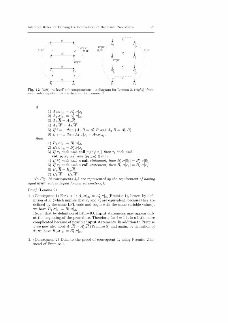
Fig. 12 (left) ‘at-level’ subcomputations – a diagram for Lemma 2. (right) ‘from-level’ subcomputations – a diagram for Lemma 3

if1) A1.σ|d1 = A′1.σ|d1

2) A2.σ|d2 = A′2.σ|d2

3) A1.R = A2.R4) A1.W = A2.W5) If i = 1 then (A1.R = A′1.R and A2.R = A′2.R)6) If i = 1 then A1.σ|d1 = A2.σ|d2 .

then1) B1.σ|d1 = B′

1.σ|d1

2) B2.σ|d2 = B′2.σ|d2

3) If π̄i ends with call p1(e1; x1) then τ̄i ends withcall p2(e2;x2) and 〈p1, p2〉 ∈ map

4) If π̄′i ends with a call statement, then B′1.σ[e1] = B′

2.σ[e2]5) If π̄i ends with a call statement, then B1.σ[e1] = B2.σ[e2]6) B1.R = B2.R7) B1.W = B2.W

(In Fig. 12 consequents 4,5 are represented by the requirement of havingequal arg-r values (equal formal parameters)).

Proof (Lemma 2)1. (Consequent 1) For i > 1: A1.σ|d1 = A′1.σ|d1(Premise 1), hence, by defi-

nition of π̄′i (which implies that π̄i and π̄′i are equivalent, because they aredefined by the same LPL code and begin with the same variable values),we have B1.σ|d1 = B′

1.σ|d1 .Recall that by definition of LPL+IO, input statements may appear onlyat the beginning of the procedure. Therefore, for i = 1 it is a little morecomplicated because of possible input statements. In addition to Premise1 we now also need A1.R = A′1.R (Premise 5) and again, by definition ofπ̄′i we have B1.σ|d1 = B′

1.σ|d1 .

2. (Consequent 2) Dual to the proof of consequent 1, using Premise 2 in-stead of Premise 1.


3. Since π̄i, π̄′i are defined by the same LPL code and begin with the same

variable values and, for the case of i = 1, the same input sequence,they consume the same portions of the input sequence and produce thesame output subsequence. Thus, we have ∆W [π̄i] = ∆W [π̄′i],∆R[π̄i] =∆R[π̄′i], and in a similar way with respect to τ̄i, τ̄

′i , we have ∆W [τ̄i] =

∆W [τ̄ ′i ],∆R[τ̄i] = ∆R[τ̄ ′i ].

4. If i = 1, π̄i, π̄′i, τ̄

′i and τ̄i are the first segments in π, π′, τ ′ and τ , and

thus may contain input statements. Then by Premise 5 of the lemma wehave A1.R = A′1.R, A2.R = A′2.R, and by A1.R = A2.R (Premise 3) andtransitivity of equality we have A′1.R = A′2.R.

5. (Consequents 3 and 4) The subcomputations from the beginning of π′ tothe end of π̄′i and from the beginning of τ ′ to the end of τ̄ ′i are prefixes ofvalid subcomputations through FUP and GUP . These subcomputationsare input equivalent due to A′1.R = A′2.R (see item 4 above) and A1.σ|d1 =A2.σ|d2 (Premise 6). If π̄i ends with call p1(e1; x1) then π̄′i ends withcall UP(p1)(e1;x1). Then, by call-output-seq-equiv(FUP , GUP ) (premise9.4 of (react-eq)), τ̄ ′i must end with call UP(p2)(e2; x2) where 〈p1, p2〉 ∈map, and therefore τ̄i ends with call p2(e2; x2). This proves consequent3. The same premise also implies that B′

1.σ[e1] = B′2.σ[e2], which proves

consequent 4, and that ∆W [π̄′i] = ∆W [τ̄ ′i ].

6. (Consequent 5) Implied by consequents 1,2 and 4 that we have alreadyproved, and transitivity of equality.

7. Consider π̄′i and τ̄ ′i . For i = 1, π̄′1 and τ̄ ′1 are prefixes of valid input-equivalent subcomputations through FUP and GUP , and as in any suchsubcomputation the inputs are consumed only at the beginning. There-fore, input-suffix -equiv(FUP , GUP ) (Premise 9.3), which implies equalityof ∆R of these subcomputations, also implies ∆R[π̄′1] = ∆R[τ̄ ′1]. For i > 1,no input values are read in π̄′i and τ̄ ′i and hence ∆R[π̄′i] = ∆R[τ̄ ′i ] = ∅.Thus, for any i we have ∆R[π̄′i] = ∆R[τ̄ ′i ].

8. (Consequent 6) By ∆R[π̄i] = ∆R[π̄′i], ∆R[τ̄i] = ∆R[τ̄ ′i ] (see item 3),∆R[π̄′i] = ∆R[τ̄ ′i ] (see item 7) and transitivity of equality we have ∆R[π̄i] =∆R[τ̄i]. This together with A1.R = A2.R (Premise 3) entails consequent 6.

9. (Consequent 7) By ∆W [π̄i] = ∆W [π̄′i], ∆W [τ̄i] = ∆W [τ̄ ′i ] (see item 3),∆W [π̄′i] = ∆W [τ̄ ′i ] (see end of item 5) and transitivity of equality we have∆W [π̄i] = ∆W [τ̄i]. This together with A1.W = A2.W (Premise 4) entailsconsequent 7.

(End of proof of Lemma 2). utThe notations in the following lemma corresponds to the right drawing in

Fig. 12. The beginning configurations B1, B′1, B

′2, B2 are the same as the end

configurations of the drawing in the left of the same figure. In addition wenow have the configurations at the end of the ‘from-level’ subcomputations,


denoted by C1, C′1, C2, C

′2, or, more formally:

C1 = last[π̂j ], C ′1 = last[π̂′j ], C ′2 = last[τ̂ ′j ], C2 = last[τ̂j ] .

Note that π̂j is finite by definition of π, and therefore last[π̂j ] is well-defined.We will show in the proof of the next lemma that τ̂j is finite as well, andtherefore last[τ̂j ] is also well-defined.

Lemma 3 (Properties of a ‘from-level’ subcomputation) With re-spect to π̂j , τ̂j , π̂

′j and τ̂ ′j for some j, let current-label[B1] = before[cF ],

current-label[B2] = before[cG], cF = call p1(e1;x1), and cG = call p2(e2;x2).Then

if1) B1.σ|d1 = B′

1.σ|d1

2) B2.σ|d2 = B′2.σ|d2

3) B1.σ[e1] = B2.σ[e2]4) B′

1.σ[e1] = B′2.σ[e2]

5) B1.R = B2.R6) B1.W = B2.W7) π̂j has a stack-level tree of depth at most d− 18)〈p1, p2〉 ∈ map ,

then1) C1.R = C2.R2) C1.W = C2.W3) C1.σ|d1 = C ′1.σ|d1

4) C2.σ|d2 = C ′2.σ|d2

5) τ̂j has a stack-level tree of depth at most d− 1 .

Proof (Lemma 3)1. (Consequents 1,2,5) As π̂j has a stack-level tree of depth at most d − 1

(Premise 7), by B1.σ[e1] = B2.σ[e2] (Premise 3), B1.R = B2.R (Premise5), and the induction hypothesis of Lemma 1, τ̂j has stack-level treeof depth at most d − 1 and: C1.σ[x1] = C2.σ[x2], C1.R = C2.R and∆W [π̂j ] = ∆W [τ̂j ]. Therefore, by B1.W = B2.W (Premise 6) we haveC1.W = C2.W .

2. (Consequents 3,4) As π̂′j and τ̂ ′j are computations through calls to thesame uninterpreted procedure (by premise 8) we can choose them in sucha way that they satisfy C ′1.σ[x1] = C1.σ[x1] = C2.σ[x2] = C ′2.σ[x2], andhence satisfy (1). As valuations of other variables by σ|d1 and σ|d2 areunchanged by subcomputations in higher levels (above d1 and d2 respec-tively), we have C1.σ|d1 = C ′1.σ|d1 and C2.σ|d2 = C ′2.σ|d1 .

(End of proof of Lemma 3). utUsing lemmas 2 and 3 we can establish equivalences of values in the

end of input-equivalent subcomputations, based on the fact that every sub-computation, as mentioned earlier, is an interleaving between ‘at-level’ and‘from-level’ subcomputations.


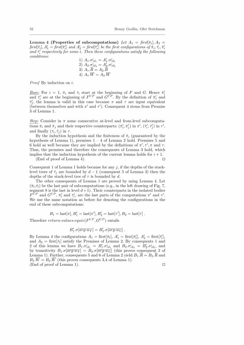
Lemma 4 (Properties of subcomputations) Let A1 = first[π̄i], A2 =first[τ̄i], A′1 = first[π̄′i] and A′2 = first[τ̄ ′i ] be the first configurations of π̄i, τ̄i, π̄

′i

and τ̄ ′i respectively for some i. Then these configurations satisfy the followingconditions:

1) A1.σ|d1 = A′1.σ|d1

2) A2.σ|d2 = A′2.σ|d2

3) A1.R = A2.R4) A1.W = A2.W

Proof By induction on i.

Base: For i = 1, π̄i and τ̄i start at the beginning of F and G. Hence π̄′iand τ̄ ′i are at the beginning of FUP and GUP . By the definition of π̄′1 andτ̄ ′1, the lemma is valid in this case because π and τ are input equivalent(between themselves and with π′ and τ ′). Consequent 4 stems from Premise3 of Lemma 1.

Step: Consider in π some consecutive at-level and from-level subcomputa-tions π̄i and π̂j and their respective counterparts: (π̄′i, π̂

′j) in π′, (τ̄ ′i , τ̂

′j) in τ ′,

and finally (τ̄i, τ̂j) in τ .By the induction hypothesis and the finiteness of π̂i (guaranteed by the

hypothesis of Lemma 1), premises 1 – 4 of Lemma 2 hold. Premises 5 and6 hold as well because they are implied by the definitions of π′, τ ′, π and τ .Thus, the premises and therefore the consequents of Lemma 3 hold, whichimplies that the induction hypothesis of the current lemma holds for i + 1.

(End of proof of Lemma 4). utConsequent 1 of Lemma 1 holds because for any j, if the depths of the stack-level trees of τ̂j are bounded by d − 1 (consequent 5 of Lemma 3) then thedepths of the stack-level tree of τ is bounded by d.

The other consequents of Lemma 1 are proved by using Lemma 4. Let(π̄l,τ̄l) be the last pair of subcomputations (e.g., in the left drawing of Fig. 7,segment 8 is the last in level d+1). Their counterparts in the isolated bodiesFUP and GUP , π̄′l and τ̄ ′l , are the last parts of the computations π′ and τ ′.We use the same notation as before for denoting the configurations in theend of these subcomputations:

B1 = last[π], B′1 = last[π′], B′

2 = last[τ ′], B2 = last[τ ] .

Therefore return-values-equiv(FUP , GUP ) entails

B′1.σ[arg-wF ] = B′

2.σ[arg-wG] .

By Lemma 4 the configurations A1 = first[π̄l], A′1 = first[π̄′l], A′2 = first[τ̄ ′l ],and A2 = first[τ̄l] satisfy the Premises of Lemma 2. By consequents 1 and2 of this lemma we have B1.σ|d1 = B′

1.σ|d1 and B2.σ|d2 = B′2.σ|d2 , and

by transitivity B1.σ[arg-wF ] = B2.σ[arg-wG] (this proves consequent 2 ofLemma 1). Further, consequents 5 and 6 of Lemma 2 yield B1.R = B2.R andB1.W = B2.W (this proves consequents 3,4 of Lemma 1).(End of proof of Lemma 1). ut


2,4 6

3 9

1

2

3

4

5

6

7

8

9 11

12 12

108,10

1,5,7

11

p1

F

B3

B1θ2θ1n1

Fig. 13 (left) A part of an infinite computation π and (right) its correspondingstack-level tree t1. The branch on the right is infinite. The notation correspond toLemma 5.

It is left to consider the case when π and τ are infinite (recall that byLemma 1 π is infinite if and only if τ is infinite). Hence, there is exactlyone infinite branch in each of the stack-level trees t1 and t2 (the stack-leveltrees of π and τ respectively). Figure 13 presents a possible part of π andits corresponding stack-level tree. Consider these infinite branches as infinitesequences of nodes, which begin at their respective roots and continue tonodes of higher levels.

We first need the following definition:

Definition 18 (Call configuration) A configuration C is a call configura-tion if current-label[C] = before[call p(e;x)] for some procedure p. ¦

Lemma 5 Let π and τ be input-equivalent infinite computations through Fand G, respectively, with corresponding stack-level trees t1 and t2. Considerthe series of call configurations which are the last in their respective levelson the infinite branches of t1 and t2 (i.e., the ones that bring the executionfrom one node of the infinite branch to the next one). Let B1 and B2 be apair of such configurations such that B1.d = B2.d and let current-label[B1] =before[call p1(e1;x1)] and current-label[B2] = before[call p2(e2;x2)]. Then

1) 〈p1, p2〉 ∈ map2) B1.σ[e1] = B2.σ[e2]3) B1.R = B2.R4) B1.W = B2.W .

As in the case of Lemma 1, if the premises do not hold (i.e., the compu-tations are not input-equivalent), Theorem 1 holds trivially. Also as in thecase of Lemma 1, consequent 4 implies OutSeq[π] = OutSeq[τ ] and hencethe consequent of Theorem 1 for the case of infinite computations.

Proof (Lemma 5) By induction on the index of the nodes in the infinitebranches. Let B1 and B2 be a pair of call configurations on the infinitebranches of t1 and t2 respectively, which are at the same execution level, i.e.,B1.d = B2.d.


Base: Consider n1, n2, the root nodes of t1 and t2. For each of the branchesoriginating from n1, n2 that are not on the infinite branches (these are nodescontaining segments (2,4) and (6) in t1, as appears in the figure), Lemma 1holds.

This allows us to use Lemma 4 (for example, between points θ1 and θ2 inthe left drawing), and Lemma 2 (for example, between points θ2 and B1 inthe left drawing) with respect to subcomputations starting in the beginningof F and G and ending at B1, B2.

By consequent 3 of Lemma 2 〈p1, p2〉 ∈ map, which proves consequent 1of the current lemma. Consequents 5,6 and 7 of Lemma 2 imply the otherthree consequents of the current lemma: B1.σ[e1] = B2.σ[e2], B1.R = B2.Rand B1.W = B2.W .

Step: Let the call configurations B3 and B4 be the successors of B1 and B2

respectively on the infinite branches. The subcomputations from B1 to B3

and from B2 to B4 are finite and therefore Lemmas 1-4 apply to them.We now assume that the induction hypothesis holds for B1 and B2 and

prove it for B3 and B4. By the induction hypothesis B1.σ[e1] = B2.σ[e2],B1.R = B2.R, and B1.W = B2.W .

Let n3 and n4 be the nodes in the stack-level trees reached by the callsmade at B1 and B2. For each of the branches originating from n3, n4 thatare not on the infinite branches Lemma 1 holds.

Similarly to the base case, Lemmas 2 and 4 apply to the subcomputationsstarting in B1 and B2 and ending at B3, B4 respectively. By consequent 3 ofLemma 2 the procedures called at B3 and B4 are mapped to one another,which proves consequent 1 of the current lemma. Consequents 5,6 and 7 ofLemma 2 imply the other three consequents of the current lemma: B3.σ[e1] =B4.σ[e2], B3.R = B4.R and B3.W = B4.W .

(End of proof of Lemma 5) utWe proved for both finite and infinite computations that the premises of

Theorem 3 imply its consequent. This concludes the proof of soundness forthe (react-eq) rule.(End of proof of Theorem 3). ut

5.4 Using rule (react-eq): a long example

Every reactive program has at least one loop or recursion, and, recall, theformer can be translated into recursion as well.

In this section we present an example of a pair of reactive programswhich behave as a simple calculator over natural numbers. The calculatedexpressions can contain the ‘+’ and ‘*’ operations and the use of ‘(’ and ‘)’to associate operations. The calculator obeys the operator precedence of ‘+’and ‘*’. We set the domain D .= N ∪ {‘+’,‘*’,‘(’,‘)’}, where ‘+’,‘*’,‘(’ and ‘)’are constant symbols, and the constants true and false to be the 1 and 0values respectively. We define + and * to be operators over D. If t1, t2 ∈ Nthen the value of t1 + t2 and t1 ∗ t2 is as given by the natural interpretation of


this operations over N. If t1 6∈ N or t2 6∈ N then we define t1 + t2 = t1 ∗ t2 = 0.We assume also the existence of the equality operator = over D.

The two programs in Fig. 14 are executed by a call to their respective“sum” procedures with 0 as the input argument. We assume that the inputsequence to the program is a valid arithmetical expression. Each time a pro-gram reads ‘)’ from the input sequence, it prints the value of the expressionbetween the parentheses that this input symbol closes. We proceed with ashort explanation of the programs’ operation.

procedure sumL(val vL; ret rL):call prodL(1; rL, opL);rL := rL + vL;if opL=‘)’ then

output(rL);

fiif opL=‘+’ then

call sumL(rL; rL)

fireturn

procedure sumR(val vR; ret rR):call prodR(1; bR, opR);if opR =‘+’ then

call sumR(vR + bR; rR)else

rR:=vR + bR;fiif opR=‘)’ then

output(vR + bR);

fireturn

procedure prodL(val vL; ret rL,opL):

call numL(rL);rL := rL ∗ vL;call getopL(opL);if opL = ‘*’ then

call prodL(rL; rL, opL)

fireturn

procedure prodR(val vR; ret rR,opR):

call numR(dR);call getopR(opR);if opR=‘*’ then

call prodR(vR ∗dR; rR, opR)else

rR := vR ∗ dR

fireturn

procedure numL(val; ret iL):input(iL);if iL=‘(’ then

call sumL(0; iL)

fireturn

procedure numR(val; ret nR):input(iR);if iR=‘(’ then

call sumR(0; nR)else

nR := iR

fireturn

procedure getopL(val; ret opL):input(opL);return

procedure getopR(val; ret opR):input(opR);return

Fig. 14 Two reactive calculator programs (labels were removed for better read-ability). The programs output a value every time they encounter the ‘)’ symbol.

The procedures sumL and sumR receive the value of the sum until nowin the formal arguments vL or vR respectively, add to it the value of the nextproduct that they receive in variable rL or bR (from calls to prodL or prodR),and if the next symbol is ‘)’ they output the sum and return it in variable


rL or rR respectively. If the next symbol is ‘+’ they recursively call sumL orsumR to continue the summation.

Similarly, the procedures prodL and prodR receive the value of the productup to now in formal argument vL and vR, multiply it by the value of the nextnatural number or expression in parentheses (received from numL or numR

in variable rL or dR), and get the next symbol in opL or opR. If the nextsymbol is ‘*’ they recursively call prodL or prodR to continue calculating theproduct. If the next symbol is ‘+’ or ‘)’, they just return the product value(in rL or rR).

The numL and numR procedure may read a number or a ‘(’ symbol fromthe input sequence. In the former case, they just return this number throughiL or nR. In the latter case, they call sumL and sumR to calculate the valueof the expression inside the parentheses and return the result through iL ornR.

The getopL and getopR just read a single symbol from the input sequence(it can be ‘+’, ‘*’ or ‘)’) and return it in opL or opR, respectively.

We use the (react-eq) rule to prove reactive equivalence of sumL andsumR, under the assumption that they receive a valid arithmetical expres-sion. We introduce four uninterpreted procedures Us, Up, Un and Ug and setthe mapping UP to satisfy UP (sumL) = UP (sumR) = Us, UP (prodL) =UP (prodR) = Up, UP (numL) = UP (numR) = Un and UP (getopL) =UP (getopR) = Ug.

In Fig. 15 we present the SSA form of the formulas that represent thepossible computations of the isolated procedure bodies. Each of the proce-dures has at most a single input or output statement. We mark the singleinput value by in1 or in2, and the single output value by out1 or out2.

– Premise 9.2 (return-values-equiv). Checking this premise involveschecking all input-equivalent subcomputations through the isolated bod-ies of each pair of the related procedures. As each of these isolated bodiesinclude at most a single input statement, a sequence of a single input isenough for each of these checks. We denote this single input by R0. Wecheck the following formulas to be valid:

(vL = vR ∧ TsumL ∧ TsumR) → rL = rR

(vL = vR ∧ TprodL ∧ TprodR) → rL = rR ∧ opL = opR

(in1 = R0 ∧ in2 = R0 ∧ TnumL ∧ TnumR) → iL = nR

(in1 = R0 ∧ in2 = R0 ∧ TgetopL ∧ TgetopR) → opL = opR .

(10)

– Premise 9.3 (input-suffix -equiv). Recall that calls to uninterpretedprocedures consume no values of the input sequence. Thus, to verify thesatisfaction of input-suffix -equiv , we only need to check that any two re-lated procedures have the same number of input statements. In this way,when the configurations at the beginning of the two isolated procedurebodies have equal input sequences, also the configurations at the end ofthese bodies have equal input sequences as the same prefix was consumedby the computations through the bodies. This condition is satisfied triv-ially for all mapped procedures.


vL0 = vL ∧

Up(1; rL1 , opL

1) ∧rL2 = rL

1 + vL0 ∧

(opL1 = ‘)’ → out1 = rL

2 ) ∧(opL

1 = ‘+’ → Us(rL2 ; rL

3 )) ∧(opL

1 6= ‘+’ → rL3 = rL

2 ) ∧rL = rL

3

vR0 = vR ∧

Up(1; bR1 , opR

1 ) ∧

(opR1 = ‘+’ → Us(v

R0 + bR

1 ; rR1 )) ∧

(opR1 6= ‘+’ → rR

1 = vR0 + bR

1 ) ∧(opR

1 = ‘)’ → out2 = vR0 + bR

1 ) ∧rR = rR

1

TsumL TsumR

vL0 = vL ∧

Un(rL1 ) ∧

rL2 = rL

1 ∗ vL0 ∧

Ug(opL1) ∧

(opL1 = ‘*’ → Up(rL

2 ; rL3 , opL

2)) ∧(opL

1 6= ‘*’ → (rL3 = rL

2∧opL

2 = opL1)) ∧

rL = rL3 ∧ opL = opL

2

vR0 = vR ∧

Un(dR1 ) ∧

Ug(opR1 ) ∧

(opR1 = ‘*’ → Up(vR

0 ∗ dR1 ;

rR1 , opR

2 )) ∧(opR

1 6= ‘*’ → (rR1 = vR

0 ∗ dR1∧

opR2 = opR

1 )) ∧rR = rR

1 ∧ opR = opR2

TprodL TprodR

iL0 = in1 ∧(iL0 = ‘(’ → Us(0; iL1)) ∧(iL0 6= ‘(’ → iL1 = iL0) ∧iL = iL1

iR0 = in2 ∧(iR0 = ‘(’ → Us(0; nR

1 )) ∧(iR0 6= ‘(’ → nR

1 = iR0 ) ∧nR = nR

1

TnumL TnumR

(opL

0 = in1 ∧opL = opL

0

) (opR

0 = in2 ∧opR = opR

0

)

TgetopL TgetopR

Fig. 15 The SSA corresponding to the programs in Fig. 14.

– Premise 9.4 (call-output-seq-equiv). In procedures sumL, sumR, prodL,prodR, numL and numR, the execution may take several paths. We needto compare the guard and input values of each procedure call and eachoutput statement in each path. Note that the calls to Un and Ug are al-ways unconditioned and have no read arguments. Therefore, they triviallysatisfy the call-output-seq-equiv conditions. The check involves validatingthe following formulas:

(vL = vR ∧ TsumL ∧ TsumR) →((1 = 1) ∧(opL

1 = ‘)’ ↔ opR1 = ‘)’) ∧ (opL

1 = ‘)’ → out1 = out2) ∧(opL

1 = ‘+’ ↔ opR1 = ‘+’) ∧ (opL

1 = ‘+’ → rL2 = vR

0 + bR1 )) .

(11)

It is easier to follow this formula while referring to the definition of TsumL

and TsumR . The second line asserts that the input arguments of Up arethe same. The third line asserts that the guards of the output statementsare the same, and if they both hold, then the output value is the same.The last line asserts that the guards of the call to Us are the same, andif they both hold, then the read arguments of Us are the same.

(vL = vR ∧ TprodL ∧ TprodR) →((opL

1 = ‘*’ ↔ opR1 = ‘*’) ∧ (opL

1 = ‘*’ → rL2 = vR

0 ∗ dR1 )) (12)


(in1 = R0 ∧ in2 = R0 ∧ TnumL ∧ TnumR) →((iL0 = ‘(’ ↔ iR0 = ‘(’) ∧ (iL0 = ‘(’ → 0 = 0)) .

(13)

Using the uninterpreted procedure relations and commutativity of the ‘+’and ‘*’ operators, one can prove the validity of (10) – (13). Note that unin-terpreted procedures which have no read arguments return non-deterministicbut constant values in their write arguments.

This concludes the verification of the premises of rule (react-eq), whichestablishes, among other things, that reactive-equiv(sumL, sumR) holds.Consequently we know that the two programs generate the same outputsequence when executed on the same arithmetical expression.

6 What the rules cannot prove

All three rules rely on a 1-1 and onto mapping of the procedures (possiblyafter inlining of some of them, as mentioned in the introduction), such thatevery pair of mapped procedures are computationally equivalent. Varioussemantic-preserving code transformations do not satisfy this requirement.Here are a few examples:

1. Consider the following equivalent procedures, which, for a natural numbern, compute

∑ni=1 i.

procedure F(val n; ret r):if n ≤ 1 then r := nelse

call F (n− 1, r);r := n + r

fireturn

procedure G(val n; ret r):if n ≤ 1 then r := nelse

call G(n− 2, r);r := n + (n− 1) + r

fireturn

Since the two procedures are called with different arguments, their com-putational equivalence cannot be proven with rule (proc-p-eq).

2. Consider a similar pair of equivalent procedures, that this time makerecursive calls with equivalent arguments:

procedure F(val n; ret r):if n ≤ 0 then r := nelse

call F (n− 1, r);r := n + r

fireturn

procedure G(val n; ret r):if n ≤ 1 then r := nelse

call G(n− 1, r);r := n + r

fireturn

The premise of (proc-p-eq) fails due to the case of n == 1.3. We now consider an example in which the two programs are both compu-

tational equivalent and reach-equivalent, but still our rules fail to proveit.


procedure F(val n; ret r):if n ≤ 0 then r := 0else

call F (n− 1, r);r := n + r

fi;return

procedure F(val n; ret r):if n ≤ 0 then r := 0else

call F (n− 1, r);if r ≥ 0 then r := n + r;fi

fireturn

In this case the ‘if’ condition in the second program always holds. Yetsince the Uninterpreted Functions return arbitrary, although equal, val-ues, they can return a negative value, which will make this ‘if’ conditionnot hold and as a result make the two isolated functions return differentvalues.

7 Summary

We presented three proof rules in the style of Hoare’s rule for recursive pro-cedures: rule (proc-p-eq) proves partial equivalence between programs, rule(m-term) proves mutual termination of such programs and, finally, rule(react-eq) proves reactive-equivalence between reactive programs, and alsogeneralizes the first two.

These rules can be used in any one of the scenarios described in the intro-duction. We are using them as part of an automated regression-verificationtool for C programs that we currently develop, and so far used them forproving such equivalence of several non-trivial programs. Deriving the properverification conditions automatically is easy in the isolated procedures, andthe verification conditions themselves are typically not hard to solve withthe underlying proof engine that we use, namely CBMC8. Once this systemwill be capable of handling a larger set of real programs (it currently doesnot support various language features of C), it will be interesting to see inhow many cases real changes, made between versions of real programs, canbe proven to be equal with the rules described in this article.

References

1. Arons, T., Elster, E., Fix, L., MadorHaim, S., Mishaeli, M., Shalev, J., Singer-man, E., Tiemeyer, A., Vardi, M.Y., , Zuck, L.D.: Formal verification of back-ward compatibility of microcode. In: K. Etessami, S. Rajamani (eds.) Proc.17th Intl. Conference on Computer Aided Verification (CAV’05), Lect. Notesin Comp. Sci., vol. 3576. Springer-Verlag, Edinburgh (2005)

2. Bouge, L., Cachera, D.: A logical framework to prove properties of al-pha programs (revised version). Tech. Rep. RR-3177 (1997). URL cite-seer.ist.psu.edu/bouge97logical.html

8 This depends more on the type of operators there are in the procedures thanthe sheer size of the program. For example, a short program that includes a mul-tiplication between two integers is hard to reason about regardless of the length ofthe procedure.


3. Cytron, R., Ferrante, J., Rosen, B.K., Wegman, M.N., Zadeck, F.K.: Efficientlycomputing static single assignment form and the control dependence graph.ACM Transactions on Programming Languages and Systems 13(4), 451–490(1991)

4. Fowler, M.: http://www.refactoring.com5. Fowler, M.: Refactoring: Improving the Design of Existing Code. Addison-

Wesley (1999)6. Francez, N.: Program Verification. Addison-Wesley (1993)7. Hoare, C.: Procedures and parameters: an axiomatic approach. In Proc. Sym.

on semantics of algorithmic languages (188) (1971)8. Kroening, D., Clarke, E., Yorav, K.: Behavioral consistency of C and Verilog

programs using bounded model checking. In: Proceedings of DAC 2003, pp.368–371. ACM Press (2003)

9. Luckham, D.C., Park, M.R., Paterson, M.S.: On formalized computer pro-grams. Jour. Comp. and System Sciences 4(3) (1970)

10. Manolios, P.: Computer-Aided Reasoning: ACL2 Case Studies, chap. Mu-Calculus Model-Checking, pp. 93–111. Kluwer Academic Publishers (2000)

11. Manolios, P., Kaufmann, M.: Adding a total order to acl2. In: The ThirdInternational Workshop on the ACL2 Theorem Prover (2002)

12. Manolios, P., Vroon, D.: Ordinal arithmetic: Algorithms and mechanization.Journal of Automated Reasoning (2006). To appear

13. Pratt, T.W.: Kernel equivalence of programs and proving kernel equivalenceand correctness by test cases. International Joint Conference on ArtificialIntelligence (1971)

14. Shostak, R.: An algorithm for reasoning about equality. Communications ofthe ACM 21(7), 583 – 585 (1978)

A Formal definitions for Section 5

Definition 19 (Input/output subsequences of a subcomputation)Let π′ be a subcomputation of a computation π. If π′ is finite then the inputsubsequence of π′ is the prefix sequence QIN that satisfies first[π′].R = QIN ·last[π′].R and the output subsequence of π′ is the tail sequence QOUT that satisfies

first[π′].W ·QOUT = last[π′].W . If π′ is infinite then the input subsequence of π′ is

simply first[π′].R and the output subsequence of π′ is the tail sequence QOUT that

satisfies first[π′].W ·QOUT = OutSeq[π]. ¦Less formally, an input subsequence of a subcomputation π′ is the subsequence ofinputs that is ‘consumed’ by π′, whereas the output subsequence of a subcompu-tation π′ is the subsequence of outputs of π′.

We mark the input subsequence of π′ by ∆R[π′] and its output subsequence by

∆W [π′].In all subsequent definitions P1 and P2 are LPL+IO programs.

Definition 20 (Reactive equivalence of two procedures)Given two procedures F ∈ Proc[P1] and G ∈ Proc[P2] such that 〈F, G〉 ∈ map, iffor every two subcomputations π′1 and π′2 that are input equivalent with respect toF and G it holds that ∆W [π′1] = ∆W [π′2] then F and G are reactively equivalent.¦Denote by reactive-equiv(F, G) the fact that F and G are reactively equivalent.

Definition 21 (Return-values equivalence of two reactive procedures)If for every two finite subcomputations π′1 and π′2 that are input equivalent withrespect to procedures F and G it holds that

last[π′1].σ[arg-wF ] = last[π′2].σ[arg-wG]

then F and G are Return-values equivalent. ¦


(Recall that input-equivalent subcomputations are also argument-equivalent andhence maximal – see Definition 9).

Denote by return-values-equiv(F, G) the fact that F and G are return-valueequivalent.

Definition 22 (Inputs-suffix equivalence of two reactive procedures)If for every two finite subcomputations π′1 and π′2 that are input equivalent withrespect to procedures F and G it holds that

∆R[π′1] = ∆R[π′2] ,

then F and G are Inputs-suffix equivalent. ¦

Denote by input-suffix -equiv(F, G) the fact that F and G are inputs-suffix equiva-lent.

Definition 23 (Output configuration) A configuration C is an output config-uration if current-label[C] = before[output(e)]. ¦

Definition 24 (Call and output sequence of a subcomputation) The calland output sequence of a subcomputation π′ contains all the call and output con-figurations in π′ in the order in which they appear in π′. ¦

Definition 25 (Call and output sequence equivalence between subcom-putations) Finite subcomputation π′1 and π′2 from some levels are call and outputsequence equivalent if the call-and-output-sequences CC1 of π′1 and CC2 of π′2,satisfy:

1. |CC1| = |CC2|2. If for some i ∈ {1, . . . , |CC1|}, current-label[(CC1)i] = before[call p1(e1; x1)]),

then

– current-label[(CC2)i] = before[call p2(e2; x2)],– 〈p1, p2〉 ∈ map, and– (CC1)i.σ[e1] = (CC2)i.σ[e2].

3. If for some i ∈ {1, . . . , |CC1|}) current-label[(CC1)i] = before[output(e1)]),then– current-label[(CC2)i] = before[output(e2)], and– (CC1)i.σ[e1] = (CC2)i.σ[e2].

¦

Extending this definition to procedures, we have:

Definition 26 (Call and output sequence equivalence of two procedures)Given two procedures F ∈ Proc[P1] and G ∈ Proc[P2] such that 〈F, G〉 ∈ map,if for every two finite subcomputations π′1 and π′2 that are input equivalent withrespect to F and G it holds that π′1 and π′2 are call and output sequence equivalent,then F and G are call and output sequence equivalent. ¦

Denote by call-output-seq-equiv(F, G) the fact that F and G are call-sequenceequivalent.


B Refactoring rules that our rules can handle

It is beneficial to categorize refactoring rules that can be handled by our proofrules. In general, every change that is local to the procedure, and does not movecode between different iterations of a loop or recursion, can be handled by the proofrules.

Considering the list of popular refactoring rules in [4] (while ignoring those thatare specific to object-oriented code, or Java):

– Our rules can handle the following rules: Consolidate Duplicate ConditionalFragments, Introduce Explaining Variable, Reduce Scope of Variable, RemoveAssignments to Parameters, Remove Control Flag, Remove Double Negative,Replace Assignment with Initialization, Replace Iteration with Recursion, Re-place Magic Number with Symbolic Constant, Replace Nested Conditional withGuard Clauses, Replace Recursion with Iteration, Reverse Conditional, SplitTemporary Variable, Substitute Algorithm.

– If the rules are used in a decision procedure that is able to inline code, theycan also prove the correctness of the following refactoring rules:Decompose Conditional, Extract Method, Inline Method, Inline Temp, ReplaceParameter with Explicit Methods, Replace Parameter with Method, ReplaceTemp with Query, Self Encapsulate Field, Separate Data Access Code.

– Finally, the following refactoring rules cannot be handled by our rules:Replace Static Variable with Parameter (change in the prototype of the func-tion), Separate Query from Modifier (splits a function to two functions withdifferent behaviors), Split Loop (since in our setting, loops are modeled as re-cursive functions, this transformation turns one recursive function into two).

Inference rules for proving the equivalence of recursive procedures

Documents

Transcript of Inference rules for proving the equivalence of recursive procedures