arX

iv:0

805.

1887

v1 [

mat

h.L

O]

13

May

200

8 Effective Categoricity of Equivalence Structures

FINAL DRAFT

Wesley Calvert

Department of Mathematics

University of Notre Dame

wcalvert@nd.edu

Douglas Cenzer

Department of Mathematics

University of Florida

cenzer@math.ufl.edu

Valentina Harizanov

Department of Mathematics

George Washington University

harizanv@gwu.edu

Andrei Morozov

Sobolev Institute of Mathematics

morozov@math.nsc.ru

December 30, 2013

1 Introduction

We consider only countable structures for computable languages with universeω. We identify sentences with their Godel codes. The atomic diagram of astructure A for L is the set of all quantifier-free sentences in LA, L expandedby constants for the elements in A, which are true in A. A structure is com-putable if its atomic diagram is computable. In other words, a structure Ais computable if there is an algorithm that determines for every quantifier-free formula θ(x0, . . . , xn−1) and every sequence (a0, . . . , an−1) ∈ An, whetherA � θ(a0, . . . , an−1). The elementary diagram of A is the set of all sentences ofLA that are true in A. A structure A is decidable if its elementary diagram iscomputable. For n > 0, the n-diagram of A is the set of all Σn sentences of LAthat are true in A. A structure is n-decidable if its n-diagram is computable.

A computable structure A is computably categorical if for every computableisomorphic copy B of A, there is a computable isomorphism from A onto B. Forexample, the ordered set of rational numbers is computably categorical, while

1

the ordered set of natural numbers is not. Moreover, Goncharov and Dzgoev[12] and Remmel [28] independently proved that a computable linear ordering iscomputably categorical if and only if it has only finitely many successors. Theyalso established that a computable Boolean algebra is computably categoricalif and only if it has finitely many atoms (see also LaRoche [21]). Miller [26]proved that no computable tree of height ω is computably categorical. Lempp,McCoy, Miller and Solomon [22] characterized computable trees of finite heightthat are computably categorical. Nurtazin [27] and Metakides and Nerode [24]established that a computable algebraically closed field of finite transcendencedegree over its prime field is computably categorical. Goncharov [9] and Smith[30] characterized computably categorical abelian p-groups as those that can bewritten in one of the following forms: (Z(p∞))l ⊕ G for l ∈ ω ∪ {∞} and Gfinite, or (Z(p∞))n⊕G⊕ (Z(pk))∞ , where n, k ∈ ω and G is finite. Goncharov,Lempp and Solomon [15] proved that a computable, ordered, abelian group iscomputably categorical if and only if it has finite rank. Similarly, they showedthat a computable, ordered, Archimedean group is computably categorical ifand only if it has finite rank.

For any computable ordinal α, we say that a computable structure A is∆0α categorical if for every computable structure B isomorphic to A, there is

a ∆0α isomorphism form A onto B. Lempp, McCoy, Miller and Solomon [22]

proved that for every n ≥ 1, there is a computable tree of finite height that is∆0n+1-categorical but not ∆0

n-categorical. We say that A is relatively computablycategorical if for every structure B isomorphic to A, there is an isomorphismthat is computable relative to the atomic diagram of B. Similarly, a computableA is relatively ∆0

α categorical if for every B isomorphic to A, there is an isomor-phism that is ∆0

α relative to the atomic diagram of B. Clearly, a relatively ∆0α

categorical structure is ∆0α categorical. We are especially interested in the case

when α = 2. McCoy [23] characterized, under certain restrictions, all ∆02 cate-

gorical and relatively ∆02 categorical linear orderings and Boolean algebras. For

example, a computable Boolean algebra is relatively ∆02 categorical if and only

if it can be expressed as a finite direct sum c1 ∨ . . . ∨ cn, where each ci is eitheratomless, an atom, or 1-atom. Using an enumeration result of Selivanov [29],Goncharov [10] showed that there is a computable structure that is computablycategorical but not relatively computably categorical. Using a relativized ver-sion of Selivanov’s enumeration result, Goncharov, Harizanov, Knight, McCoy,Miller and Solomon [13] showed that for each computable successor ordinal α,there is a computable structure that is ∆0

α categorical, but not relatively ∆0α

categorical.There are syntactical conditions that are equivalent to relative ∆0

α categoric-ity. The conditions involve the existence of certain families of formulas, that is,certain Scott families. Scott families come from Scott’s Isomorphism Theorem,which says that for a countable structure A, there is an Lω1ω sentence whosecountable models are exactly the isomorphic copies of A. A Scott family fora structure A is a countable family Φ of Lω1ω formulas, possibly with finitelymany fixed parameters from A, such that:

(i) Each finite tuple in A satisfies some ψ ∈ Φ;

2

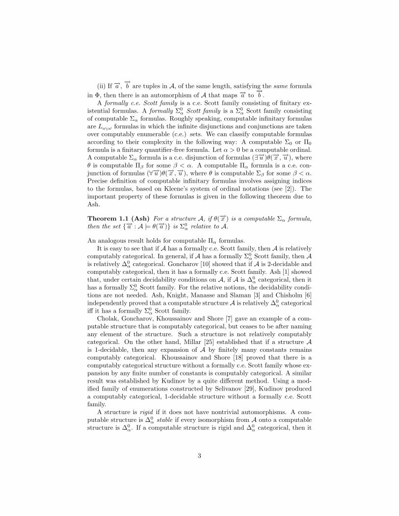
(ii) If −→a ,−→b are tuples in A, of the same length, satisfying the same formula

in Φ, then there is an automorphism of A that maps −→a to−→b .

A formally c.e. Scott family is a c.e. Scott family consisting of finitary ex-istential formulas. A formally Σ0

α Scott family is a Σ0α Scott family consisting

of computable Σα formulas. Roughly speaking, computable infinitary formulasare Lω1ω formulas in which the infinite disjunctions and conjunctions are takenover computably enumerable (c.e.) sets. We can classify computable formulasaccording to their complexity in the following way: A computable Σ0 or Π0

formula is a finitary quantifier-free formula. Let α > 0 be a computable ordinal.A computable Σα formula is a c.e. disjunction of formulas (∃−→u )θ(−→x ,−→u ), whereθ is computable Πβ for some β < α. A computable Πα formula is a c.e. con-junction of formulas (∀−→u )θ(−→x ,−→u ), where θ is computable Σβ for some β < α.Precise definition of computable infinitary formulas involves assigning indicesto the formulas, based on Kleene’s system of ordinal notations (see [2]). Theimportant property of these formulas is given in the following theorem due toAsh.

Theorem 1.1 (Ash) For a structure A, if θ(−→x ) is a computable Σα formula,then the set {−→a : A |= θ(−→a )} is Σ0

α relative to A.

An analogous result holds for computable Πα formulas.It is easy to see that if A has a formally c.e. Scott family, then A is relatively

computably categorical. In general, if A has a formally Σ0α Scott family, then A

is relatively ∆0α categorical. Goncharov [10] showed that if A is 2-decidable and

computably categorical, then it has a formally c.e. Scott family. Ash [1] showedthat, under certain decidability conditions on A, if A is ∆0

α categorical, then ithas a formally Σ0

α Scott family. For the relative notions, the decidability condi-tions are not needed. Ash, Knight, Manasse and Slaman [3] and Chisholm [6]independently proved that a computable structure A is relatively ∆0

α categoricaliff it has a formally Σ0

α Scott family.Cholak, Goncharov, Khoussainov and Shore [7] gave an example of a com-

putable structure that is computably categorical, but ceases to be after namingany element of the structure. Such a structure is not relatively computablycategorical. On the other hand, Millar [25] established that if a structure Ais 1-decidable, then any expansion of A by finitely many constants remainscomputably categorical. Khoussainov and Shore [18] proved that there is acomputably categorical structure without a formally c.e. Scott family whose ex-pansion by any finite number of constants is computably categorical. A similarresult was established by Kudinov by a quite different method. Using a mod-ified family of enumerations constructed by Selivanov [29], Kudinov produceda computably categorical, 1-decidable structure without a formally c.e. Scottfamily.

A structure is rigid if it does not have nontrivial automorphisms. A com-putable structure is ∆0

α stable if every isomorphism from A onto a computablestructure is ∆0

α. If a computable structure is rigid and ∆0α categorical, then it

3

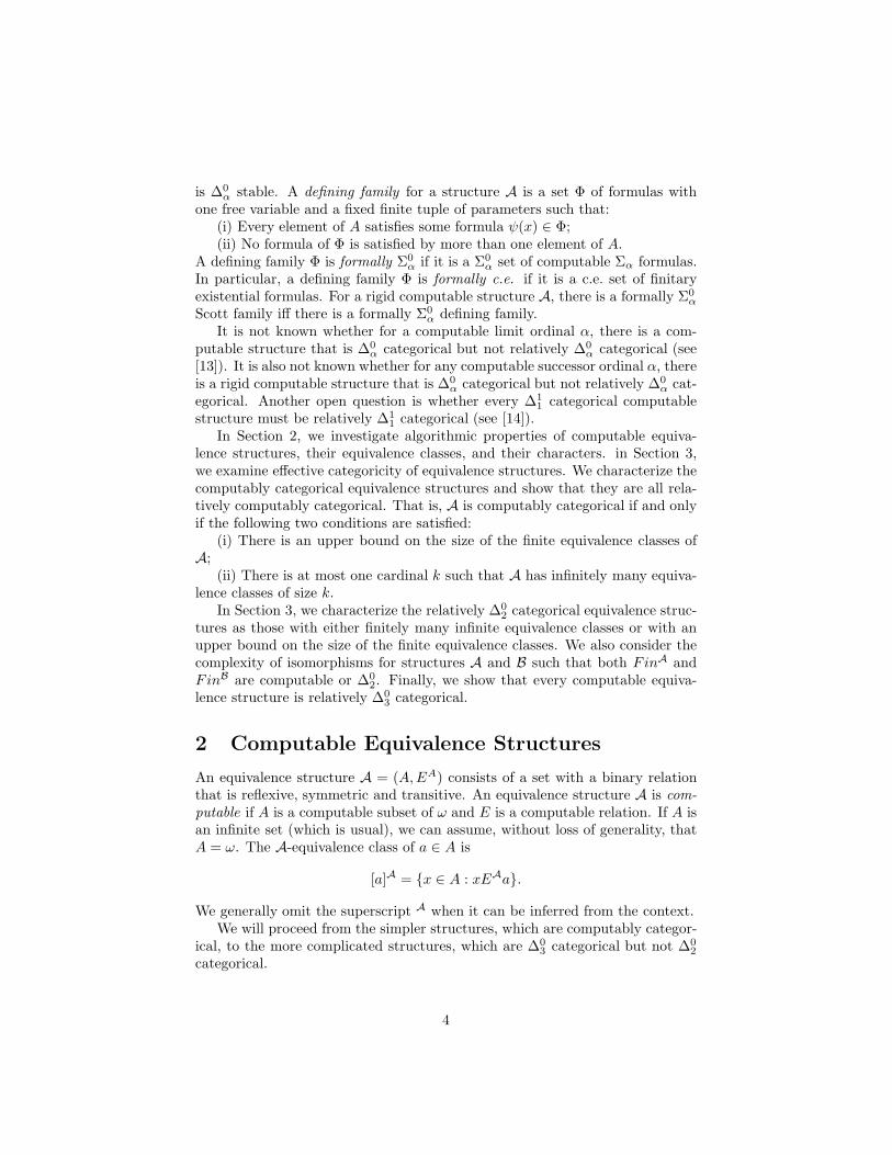
is ∆0α stable. A defining family for a structure A is a set Φ of formulas with

one free variable and a fixed finite tuple of parameters such that:(i) Every element of A satisfies some formula ψ(x) ∈ Φ;(ii) No formula of Φ is satisfied by more than one element of A.

A defining family Φ is formally Σ0α if it is a Σ0

α set of computable Σα formulas.In particular, a defining family Φ is formally c.e. if it is a c.e. set of finitaryexistential formulas. For a rigid computable structure A, there is a formally Σ0

α

Scott family iff there is a formally Σ0α defining family.

It is not known whether for a computable limit ordinal α, there is a com-putable structure that is ∆0

α categorical but not relatively ∆0α categorical (see

[13]). It is also not known whether for any computable successor ordinal α, thereis a rigid computable structure that is ∆0

α categorical but not relatively ∆0α cat-

egorical. Another open question is whether every ∆11 categorical computable

structure must be relatively ∆11 categorical (see [14]).

In Section 2, we investigate algorithmic properties of computable equiva-lence structures, their equivalence classes, and their characters. in Section 3,we examine effective categoricity of equivalence structures. We characterize thecomputably categorical equivalence structures and show that they are all rela-tively computably categorical. That is, A is computably categorical if and onlyif the following two conditions are satisfied:

(i) There is an upper bound on the size of the finite equivalence classes ofA;

(ii) There is at most one cardinal k such that A has infinitely many equiva-lence classes of size k.

In Section 3, we characterize the relatively ∆02 categorical equivalence struc-

tures as those with either finitely many infinite equivalence classes or with anupper bound on the size of the finite equivalence classes. We also consider thecomplexity of isomorphisms for structures A and B such that both FinA andFinB are computable or ∆0

2. Finally, we show that every computable equiva-lence structure is relatively ∆0

3 categorical.

2 Computable Equivalence Structures

An equivalence structure A = (A,EA) consists of a set with a binary relationthat is reflexive, symmetric and transitive. An equivalence structure A is com-putable if A is a computable subset of ω and E is a computable relation. If A isan infinite set (which is usual), we can assume, without loss of generality, thatA = ω. The A-equivalence class of a ∈ A is

[a]A = {x ∈ A : xEAa}.

We generally omit the superscript A when it can be inferred from the context.We will proceed from the simpler structures, which are computably categor-

ical, to the more complicated structures, which are ∆03 categorical but not ∆0

2

categorical.

4

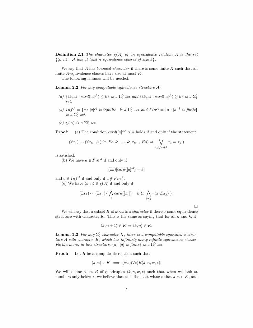
Definition 2.1 The character χ(A) of an equivalence relation A is the set{〈k, n〉 : A has at least n equivalence classes of size k}.

We say that A has bounded character if there is some finite K such that allfinite A-equivalence classes have size at most K.

The following lemmas will be needed.

Lemma 2.2 For any computable equivalence structure A:

(a) {〈k, a〉 : card([a]A) ≤ k} is a Π01 set and {〈k, a〉 : card([a]A) ≥ k} is a Σ0

1

set.

(b) InfA = {a : [a]A is infinite} is a Π02 set and FinA = {a : [a]A is finite}

is a Σ02 set.

(c) χ(A) is a Σ02 set.

Proof: (a) The condition card([a]A) ≤ k holds if and only if the statement

(∀x1) · · · (∀xk+1) ( (x1Ea & · · · & xk+1 Ea) ⇒∨

i,j 6=k+1

xi = xj )

is satisfied.(b) We have a ∈ FinA if and only if

(∃k)[card([a]A) = k]

and a ∈ InfA if and only if a /∈ FinA.(c) We have 〈k, n〉 ∈ χ(A) if and only if

(∃x1) · · · (∃xn) (∧

i

card([xi]) = k &∧

i6=j

¬(xiExj) ) .

�

We will say that a subsetK of ω×ω is a character if there is some equivalencestructure with character K. This is the same as saying that for all n and k, if

〈k, n+ 1〉 ∈ K ⇒ 〈k, n〉 ∈ K.

Lemma 2.3 For any Σ02 character K, there is a computable equivalence struc-

ture A with character K, which has infinitely many infinite equivalence classes.Furthermore, in this structure, {a : [a] is finite} is a Π0

1 set.

Proof: Let R be a computable relation such that

〈k, n〉 ∈ K ⇐⇒ (∃w)(∀z)R(k, n, w, z).

We will define a set B of quadruples 〈k, n, w, z〉 such that when we look atnumbers only below z, we believe that w is the least witness that k, n ∈ K, and

5

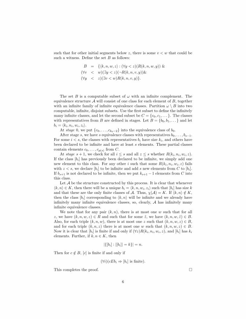
such that for other initial segments below z, there is some v < w that could besuch a witness. Define the set B as follows:

B = {〈k, n, w, z〉 : (∀y < z)(R(k, n, w, y)) &

(∀v < w)(∃y < z)(¬R(k, n, v, y))&

(∀y < z)(∃v < w)R(k, n, v, y)}.

The set B is a computable subset of ω with an infinite complement. Theequivalence structure A will consist of one class for each element of B, togetherwith an infinite family of infinite equivalence classes. Partition ω \ B into twocomputable, infinite, disjoint subsets. Use the first subset to define the infinitelymany infinite classes, and let the second subset be C = {c0, c1, . . . }. The classeswith representatives from B are defined in stages. Let B = {b0, b1, . . . } and letbi = 〈ki, ni, wi, zi〉.

At stage 0, we put {c0, . . . , ck0−2} into the equivalence class of b0.After stage s, we have s equivalence classes with representatives b0, . . . , bs−1.

For some i < s, the classes with representatives bi have size ki, and others havebeen declared to be infinite and have at least s elements. These partial classescontain elements c0, . . . , cp(s) from C.

At stage s+ 1, we check for all i ≤ s and all z ≤ s whether R(ki, ni, wi, z).If the class [bi] has previously been declared to be infinite, we simply add onenew element to this class. For any other i such that some R(ki, ni, wi, z) failswith z < s, we declare [bi] to be infinite and add s new elements from C to [bi].If bs+1 is not declared to be infinite, then we put ks+1 − 1 elements from C intothis class.

Let A be the structure constructed by this process. It is clear that whenever〈k, n〉 ∈ K, then there will be a unique bi = 〈k, n, wi, zi〉 such that [bi] has size kand that these are the only finite classes of A. Thus, χ(A) = K. If 〈k, n〉 /∈ K,then the class [bi] corresponding to 〈k, n〉 will be infinite and we already haveinfinitely many infinite equivalence classes, so, clearly, A has infinitely manyinfinite equivalence classes.

We note that for any pair (k, n), there is at most one w such that for allz, we have (k, n, w, z) ∈ R and such that for some z, we have (k, n, w, z) ∈ B.Also, for each triple (k, n, w), there is at most one z such that (k, n, w, z) ∈ B,and for each triple (k, n, z) there is at most one w such that (k, n, w, z) ∈ B.Now it is clear that [bi] is finite if and only if (∀z)R(ki, ni, wi, z), and [bi] has kielements. Further, if k, n ∈ K, then

|{[bi] : |[bi]| = k}| = n.

Then for c /∈ B, [c] is finite if and only if

(∀i)(cEbi ⇒ [bi] is finite).

This completes the proof. �

6

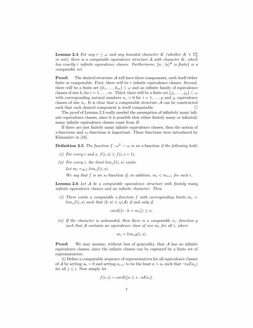
Lemma 2.4 For any r ≤ ω and any bounded character K (whether K ∈ Σ02

or not), there is a computable equivalence structure A with character K, whichhas exactly r infinite equivalence classes. Furthermore, {a : [a]A is finite} is acomputable set.

Proof: The desired structure A will have three components, each itself eitherfinite or computable. First, there will be r infinite equivalence classes. Second,there will be a finite set {k1, . . . , km} ⊂ ω and an infinite family of equivalenceclasses of size ki for i = 1, . . . ,m. Third, there will be a finite set {j1, . . . , jp} ⊂ ωwith corresponding natural numbers ni > 0 for i = 1, . . . , p and ji equivalenceclasses of size ni. It is clear that a computable structure A can be constructedsuch that each desired component is itself computable. �

The proof of Lemma 2.3 really needed the assumption of infinitely many infi-nite equivalence classes, since it is possible that either finitely many or infinitelymany infinite equivalence classes come from B.

If there are just finitely many infinite equivalence classes, then the notion ofs-functions and s1-functions is important. These functions were introduced byKhisamiev in [16].

Definition 2.5 The function f : ω2 → ω is an s-function if the following hold:

(i) For every i and s, f(i, s) ≤ f(i, s+ 1).

(ii) For every i, the limit limsf(i, s) exists.

Let mi =def limsf(i, s).

We say that f is an s1-function if, in addition, mi < mi+1 for each i.

Lemma 2.6 Let A be a computable equivalence structure with finitely manyinfinite equivalence classes and an infinite character. Then

(i) There exists a computable s-function f with corresponding limits mi =limsf(i, s) such that 〈k, n〉 ∈ χ(A) if and only if

card({i : k = mi}) ≥ n.

(ii) If the character is unbounded, then there is a computable s1 -function gsuch that A contains an equivalence class of size mi for all i, where

mi = limsg(i, s).

Proof: We may assume, without loss of generality, that A has no infiniteequivalence classes, since the infinite classes can be captured by a finite set ofrepresentatives.

(i) Define a computable sequence of representatives for all equivalence classesof A by setting a0 = 0 and setting ai+1 to be the least a > ai such that ¬(aEaj)for all j ≤ i. Now simply let

f(i, s) = card({a ≤ s : aEai}.

7

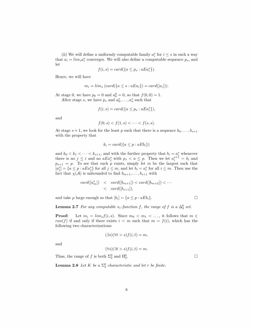
(ii) We will define a uniformly computable family asi for i ≤ s in such a waythat ai = limsa

si converges. We will also define a computable sequence ps, and

letf(i, s) = card({a ≤ ps : aEasi }).

Hence, we will have

mi = lims (card({a ≤ s : aEai}) = card([ai])).

At stage 0, we have p0 = 0 and a00 = 0, so that f(0, 0) = 1.

After stage s, we have ps and as0, . . . , ass such that

f(i, s) = card({a ≤ ps : aEasi }),

andf(0, s) < f(1, s) < · · · < f(s, s).

At stage s+ 1, we look for the least p such that there is a sequence b0, . . . , bs+1

with the property that

ki = card({a ≤ p : aEbi})

and k0 < k1 < · · · < ks+1, and with the further property that bi = asi wheneverthere is no j ≤ i and no aEasj with ps < a ≤ p. Then we let as+1

i = bi andps+1 = p. To see that such p exists, simply let m be the largest such that[asj ] = {a ≤ p : aEasj} for all j ≤ m, and let bi = asi for all i ≤ m. Then use thefact that χ(A) is unbounded to find bm+1, . . . , bs+1 with

card([asm]) < card([bm+1]) < card([bm+2]) < · · ·

< card([bs+1]),

and take p large enough so that [bi] = {a ≤ p : aEbi}. �

Lemma 2.7 For any computable s1-function f , the range of f is a ∆02 set.

Proof: Let mi = limsf(i, s). Since m0 < m1 < . . . , it follows that m ∈ran(f) if and only if there exists i < m such that m = f(i), which has thefollowing two characterizations:

(∃s)(∀t > s)f(i, t) = m,

and(∀s)(∃t > s)f(i, t) = m.

Thus, the range of f is both Σ02 and Π0

2. �

Lemma 2.8 Let K be a Σ02 characteristic and let r be finite.

8

(i) Let f be a computable s-function with the corresponding limits mi =limsf(i, s) such that 〈n, k〉 ∈ K if and only if

card({i : k = mi}) ≥ n.

Then there is a computable equivalence structure A with χ(A) = K andwith exactly r infinite equivalence classes.

(ii) Let f be a computable s1-function with corresponding limitsmi = limsf(i, s)such that 〈mi, 1〉 ∈ K for all i. Then there is a computable equivalencestructure A with χ(A) = K and exactly r infinite equivalence classes.

Proof: Clearly, it suffices to prove the statements for r = 0. We may assumethat f(i, 0) ≥ 1 for all i.

(i) Let ai = 2i. We will build an equivalence structure A with equivalenceclasses [ai] ofmi. At stage 0, make the elements 1, 3, . . . , 2(f (0, 0)−1) equivalentto a0. After stage s, we have exactly f (m, s) elements equivalent to am for eachm ≤ s. Then we add f(m, s+ 1) − f(m, s) elements to [am] for m ≤ s and putf(s+ 1, s+ 1) − 1 elements into the class of as+1.

(ii) Since there is an s1-function, the character K must be unbounded. Wemodify the argument for Lemma 2.3 as follows. The pool of elements to putinto the equivalence classes is now simply ω \B.

Here is the first modification. When we find ¬R(ki, ni, wi, z) for some z atstage s + 1, we can no longer create an infinite equivalence class, but we havealready put ki elements in the equivalence class of bi. So we will set this bloc [bi]aside until we find a number j and a stage s such that ki ≤ f(j, s). Since thereis an increasing sequence m0 < m1 < · · · corresponding to the s1-function,such j and s will eventually be found. Then we will assign a marker j to biand add f(j, s) − ki elements to the bloc to create an equivalence class withf(j, s) elements. If at a later stage t we have f(j, t) > f(j, s), then we will addf(j, t) − f(j, s) more elements to the class. Since limsf(j, s) = mj converges,we will eventually have an equivalence class of size mj .

This means that we may have created an extra equivalence class with f(j, s)elements, so the second modification is that when we create a class with k =f(j, s) elements, we may need (perhaps temporarily) to remove from our con-struction any class corresponding to 〈k, 1, w, z〉. That is, we set these (finitelymany) blocs aside to be put into a larger class, just as if we had found that¬R(k, n, w, z), but we make a note that they may need to be revived later. Ifat some later stage t, we find k′ such that

k′ = f(j, t) > f(j, s) = k,

so that we will increase the size of the class with marker j, then we are goingto remove the classes corresponding to 〈k′, 1〉 and at the same time revive theclasses corresponding to 〈k, 1〉. At this stage, we remove the attachment tof(j, s) of the bloc and check to see for all bi = 〈k, 1, w, z〉:

9

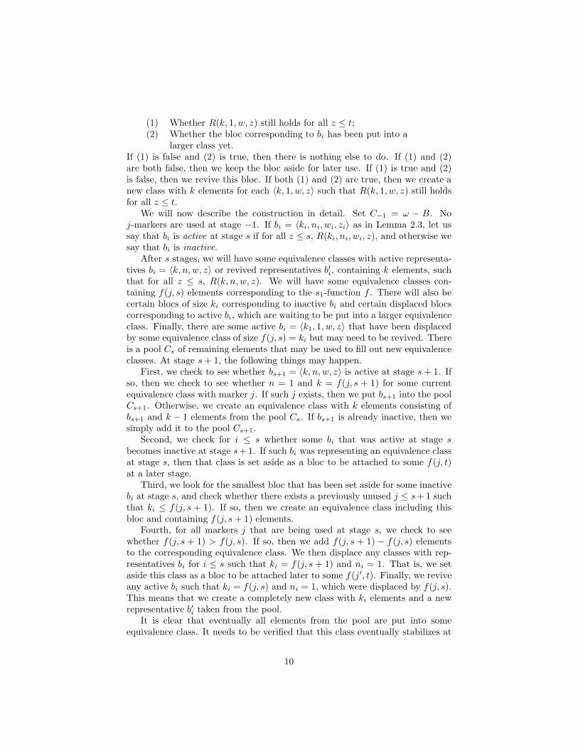
(1) Whether R(k, 1, w, z) still holds for all z ≤ t;(2) Whether the bloc corresponding to bi has been put into a

larger class yet.If (1) is false and (2) is true, then there is nothing else to do. If (1) and (2)are both false, then we keep the bloc aside for later use. If (1) is true and (2)is false, then we revive this bloc. If both (1) and (2) are true, then we create anew class with k elements for each 〈k, 1, w, z〉 such that R(k, 1, w, z) still holdsfor all z ≤ t.

We will now describe the construction in detail. Set C−1 = ω − B. Noj-markers are used at stage −1. If bi = 〈ki, ni, wi, zi〉 as in Lemma 2.3, let ussay that bi is active at stage s if for all z ≤ s, R(ki, ni, wi, z), and otherwise wesay that bi is inactive.

After s stages, we will have some equivalence classes with active representa-tives bi = 〈k, n, w, z〉 or revived representatives b′i, containing k elements, suchthat for all z ≤ s, R(k, n, w, z). We will have some equivalence classes con-taining f(j, s) elements corresponding to the s1-function f . There will also becertain blocs of size ki corresponding to inactive bi and certain displaced blocscorresponding to active bi, which are waiting to be put into a larger equivalenceclass. Finally, there are some active bi = 〈k1, 1, w, z〉 that have been displacedby some equivalence class of size f(j, s) = ki but may need to be revived. Thereis a pool Cs of remaining elements that may be used to fill out new equivalenceclasses. At stage s+ 1, the following things may happen.

First, we check to see whether bs+1 = 〈k, n, w, z〉 is active at stage s+ 1. Ifso, then we check to see whether n = 1 and k = f(j, s + 1) for some currentequivalence class with marker j. If such j exists, then we put bs+1 into the poolCs+1. Otherwise, we create an equivalence class with k elements consisting ofbs+1 and k − 1 elements from the pool Cs. If bs+1 is already inactive, then wesimply add it to the pool Cs+1.

Second, we check for i ≤ s whether some bi that was active at stage sbecomes inactive at stage s+1. If such bi was representing an equivalence classat stage s, then that class is set aside as a bloc to be attached to some f(j, t)at a later stage.

Third, we look for the smallest bloc that has been set aside for some inactivebi at stage s, and check whether there exists a previously unused j ≤ s+ 1 suchthat ki ≤ f(j, s + 1). If so, then we create an equivalence class including thisbloc and containing f(j, s+ 1) elements.

Fourth, for all markers j that are being used at stage s, we check to seewhether f(j, s + 1) > f(j, s). If so, then we add f(j, s + 1) − f(j, s) elementsto the corresponding equivalence class. We then displace any classes with rep-resentatives bi for i ≤ s such that ki = f(j, s + 1) and ni = 1. That is, we setaside this class as a bloc to be attached later to some f(j′, t). Finally, we reviveany active bi such that ki = f(j, s) and ni = 1, which were displaced by f(j, s).This means that we create a completely new class with ki elements and a newrepresentative b′i taken from the pool.

It is clear that eventually all elements from the pool are put into someequivalence class. It needs to be verified that this class eventually stabilizes at

10

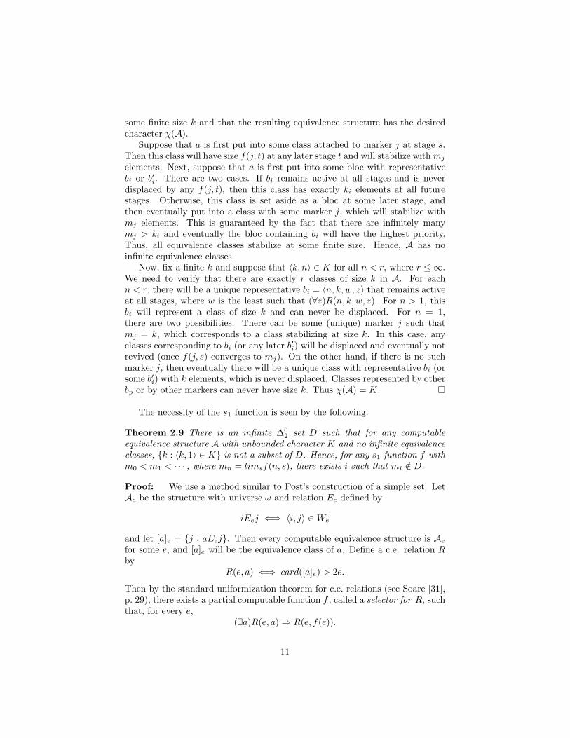
some finite size k and that the resulting equivalence structure has the desiredcharacter χ(A).

Suppose that a is first put into some class attached to marker j at stage s.Then this class will have size f(j, t) at any later stage t and will stabilize with mj

elements. Next, suppose that a is first put into some bloc with representativebi or b′i. There are two cases. If bi remains active at all stages and is neverdisplaced by any f(j, t), then this class has exactly ki elements at all futurestages. Otherwise, this class is set aside as a bloc at some later stage, andthen eventually put into a class with some marker j, which will stabilize withmj elements. This is guaranteed by the fact that there are infinitely manymj > ki and eventually the bloc containing bi will have the highest priority.Thus, all equivalence classes stabilize at some finite size. Hence, A has noinfinite equivalence classes.

Now, fix a finite k and suppose that 〈k, n〉 ∈ K for all n < r, where r ≤ ∞.We need to verify that there are exactly r classes of size k in A. For eachn < r, there will be a unique representative bi = 〈n, k, w, z〉 that remains activeat all stages, where w is the least such that (∀z)R(n, k, w, z). For n > 1, thisbi will represent a class of size k and can never be displaced. For n = 1,there are two possibilities. There can be some (unique) marker j such thatmj = k, which corresponds to a class stabilizing at size k. In this case, anyclasses corresponding to bi (or any later b′i) will be displaced and eventually notrevived (once f(j, s) converges to mj). On the other hand, if there is no suchmarker j, then eventually there will be a unique class with representative bi (orsome b′i) with k elements, which is never displaced. Classes represented by otherbp or by other markers can never have size k. Thus χ(A) = K. �

The necessity of the s1 function is seen by the following.

Theorem 2.9 There is an infinite ∆02 set D such that for any computable

equivalence structure A with unbounded character K and no infinite equivalenceclasses, {k : 〈k, 1〉 ∈ K} is not a subset of D. Hence, for any s1 function f withm0 < m1 < · · · , where mn = limsf(n, s), there exists i such that mi /∈ D.

Proof: We use a method similar to Post’s construction of a simple set. LetAe be the structure with universe ω and relation Ee defined by

iEej ⇐⇒ 〈i, j〉 ∈ We

and let [a]e = {j : aEej}. Then every computable equivalence structure is Ae

for some e, and [a]e will be the equivalence class of a. Define a c.e. relation Rby

R(e, a) ⇐⇒ card([a]e) > 2e.

Then by the standard uniformization theorem for c.e. relations (see Soare [31],p. 29), there exists a partial computable function f , called a selector for R, suchthat, for every e,

(∃a)R(e, a) ⇒ R(e, f(e)).

11

Define D as follows.

k ∈ D ⇐⇒ (∀e <k

2)(card([f(e)]e) 6= k).

Then D is a ∆02 set by part (a) of Lemma 2.2. For any ℓ, the set

D = {n|(∃x < ℓ)(n = card([f(x)]x)}

has cardinality at most ℓ, so that at most ℓ of the elements from the set{0, 1, . . . , 2ℓ} may be in D. Thus, the complement of D contains at most eelements from {0, 1, . . . , 2e}. Hence, the complement of D is infinite. Now sup-pose that A has unbounded character and has no infinite equivalence classes.Choose e so that A = Ae. Since χ(A) is unbounded, there exists a such thatR(e, a), so that a = f(e). Since A has no infinite equivalence classes,

card([a]A) = card([f(e)]e) = k > 2e

is finite. Then by definition, 〈k, 1〉 ∈ χ(A) but k /∈ D.Now let f be any s1-function, let mi = limsf(i, s), and let K = {〈mi, 1〉 :

i ∈ ω}. Then there is an equivalence structure A with character K. Therefore,some mi /∈ D. �

2.1 Computable categoricity of equivalence structures

We first investigate relative computable categoricity of computable equivalencestructures by showing that they have a formally c.e. Scott family.

Proposition 2.10 If A is a computable equivalence structure with only finitelymany finite equivalence classes, then A is relatively computably categorical.

Proof: Choose parameters c1, . . . , cn which are representatives of the n finiteequivalence classes. A Scott formula for any finite sequence −→a = a1, . . . , am ofelements from A is a conjunction of two formulas. The first formula φ(−→x ) isthe conjunction of all formulas xiExj (when aiE

Aaj) and ¬(xiExj) (when it isnot the case that aiE

Aaj). The second formula ψ(−→x ,−→c ) is the conjunction ofall formulas xiEcj (when aiE

Acj) and ¬(xiEcj) (when it is not the case thataiE

Acj). It is clear that every tuple of elements from A satisfies one of theseformulas.

Suppose that −→a and−→b satisfy the same Scott formula. Then, in particular,

we have aiEAaj ⇐⇒ biE

Abj.

For any tuple−→d , the equivalence class [di] is finite if and only if some xiE

Acj

occurs in the Scott formula of−→d , and [di] is infinite otherwise. We will define

an automorphism H of A mapping −→a to−→b .

For any equivalence class [a] containing none of the elements of −→a , of−→b , or

of −→c , the function H will simply be the identity map. We also define H(ai) = biand H(ci) = ci. This induces a partial one-to-one map from the equivalence

12

classes of A into the equivalence classes of A, which fixes finite classes setwiseand takes infinite classes to infinite classes. Within a particular finite class [ai]of size n, the partial map from [ai] to [bi] defined on [ai]∩{−→a } can be extendedto an isomorphism of [ai] onto [bi].

For the infinite classes (whether finitely or infinitely many) the partial iso-morphism of the classes may similarly be extended to a total isomorphism ofthe classes. Likewise, the partial map taking ai to bi may be extended to mapthe infinite class [ai] to the infinite class [bi]. �

Proposition 2.11 Let A be a computable equivalence structure with finitelymany infinite classes, with bounded character and with at most one finite ksuch that there are infinitely many equivalence classes of size k. Then A isrelatively computably categorical.

Proof: Let c1, . . . , cn be representatives for the finite classes not of size kand let d1, . . . , dp be representatives for the finitely many infinite classes. Thenthe Scott formula for a finite sequence −→a from A is the conjunction of threeformulas, the first two as in the proof of Proposition 2.10, and the third is theconjunction of all formulas xiEdj (when aiE

Adj) and ¬(xiEdj) (when it is notthe case that aiE

Adj). Then [ai] is infinite if and only if aiEAdj for some j,

and card([ai]) = k if and only if ¬(aiEAdj) for all j, and also ¬(aiE

Acj) for allj.

Suppose that −→a and−→b satisfy the same Scott formula. Then we can define

an automorphism of A extending the partial function which takes ai to bi as inthe proof of Proposition 2.10. �

Corollary 2.12 Let A be a computable equivalence structure of one of the fol-lowing types:

1. A has only finitely many finite equivalence classes;

2. A has finitely many infinite classes, has bounded character (i.e. only finitelymany finite sizes of equivalence classes), and has at most one finite k suchthat there are infinitely many classes of size k.

Then A is relatively computably categorical.

For structures A with FinA computable, there is a stronger result.

Proposition 2.13 Let A and B be isomorphic computable equivalence struc-tures such that FinA and FinB are computable and such that A has infinitelymany equivalence classes of size k for at most one finite k. Then A and B arecomputably isomorphic.

Proof: By Proposition 2.10, InfA and InfB are computably isomorphic andby Proposition 2.11, FinA and FinB are computably isomorphic. �

In the remainder of this section, we will show that no other equivalencestructures are computably categorical. Here is the first case.

13

Theorem 2.14 Suppose that there exist k1 < k2 ≤ ω such that the computableequivalence structure A has infinitely many equivalence classes of size k1 andinfinitely many classes of size k2. Then A is not computably categorical.

Proof: We will define structures C and D both isomorphic to A and suchthat {a : card([a]C) = k1} is a computable set, but

{a : card([a]D) = k1}

is a not computable. Then these two structures are not computably isomorphic,so A is not computably categorical.

Observe that χ(A) is a Σ02 set by part (c) of Lemma 2.2 and therefore

K = χ(A) \ {〈k1, n〉 : n < ω}

is also Σ02. Thus, if χ(A) is bounded, then there is a computable equivalence

structure with character K and the same number of infinite equivalence classesas A. If χ(A) is unbounded, then by Lemma 2.6, there is an s1-function f forχ(A). If k1 6= mi for any i, then f will be an s1-function for the character K.If k1 = mi, then define a new s1-function g for K by g(j) = f(j) for i < j,and g(j) = f(j + 1) for i ≥ j. Then there is a computable structure B withcharacter K by Lemma 2.8. Now we can define a structure C ≃ A (that is, withcharacter χ(A)) by setting

(2a+ 1) EC (2b+ 1) ⇐⇒ aEBb,

and(2(mk1 + i)) EC (2(nk1 + j)) ⇐⇒ m = n,

where i, j < k1. In this structure C, {a : card([a]) = k1} is a computable set.At the same time, we can build a structure D ≃ A such that {a : card([a]D) =

k1} is not computable. There are two cases, depending on whether k2 is finite.First suppose that k2 is finite and build a computable structure C′ with

character {〈k1, n〉, 〈k2, n〉 : n < ω} in which {a : card([a]) = k1} is a completec.e. set, as follows. Let M be a complete c.e. set and note that M is bothinfinite and co-infinite. The equivalence classes of C′ will have representatives2i so that card([2i]) = k1 if i /∈ M , and card([2i]) = k2 if i ∈ M . The oddnumbers will act as a pool of elements to fill out the classes.

The construction of C′ is in stages. After stage s, there will be classes Csicontaining 2i which will have k1 elements if i /∈ Ms and k2 elements if i ∈ Ms.At stage s+1, we add a new class containing 2s+2 and also containing k1−1 newodd elements from the pool if s+1 /∈Ms+1 and containing k2 − 1 new elementsfrom the pool if s + 1 ∈ Ms+1. Also, for any i ≤ s such that i ∈ Ms+1 \Ms,we will add k2 − k1 new elements from the pool to the class with representative[2i].

Next suppose that k2 = ω. Just modify the construction above so that wheni ∈ Ms, the class [2i] contains max{k1, s} elements. The details are left to thereader.

14

Finally we combine A and C′ into D∈ by coding A on the odd numbers andC′ on the even numbers. Then

card([2a]) = k1 ⇐⇒ a /∈M ,

so that {d : card([d]) = k1} is not computable. �

We observe that in the proof of Theorem 2.14, if FinA is computable, thenfor the case that k2 < ω, FinC and FinD will also be computable. Thus wehave the following.

Proposition 2.15 For any k1 < k2 < ω and any computable equivalence struc-ture A with FinA computable and with infinitely many equivalence classes ofsize k1 and infinitely many equivalence classes of size k2, there is a computableequivalence structure B isomorphic to A with FinB computable such that A andB are not computably isomorphic.

For the next result, we want to consider the so-called isomorphism problemfor a class of structures. For total recursive functions φe : ω × ω → {0, 1}, letCe = (ω,≡e) be the structure with

m ≡e n ⇐⇒ φe(〈m,n〉) = 1.

It is easy to check that {e : Ce is an equivalence structure} is a Π02 set. The

following Lemma is immediate from Lemma 2.2.

Convention: We say that a set is D03 if it is a difference of two Σ0

3 sets.

Lemma 2.16 (a) For any finite r,{e : Ce has at least r infinite equivalence classes} is a Σ0

3 set.

(b) For any finite r, {e : Ce has at exactly r infinite equivalence classes} is aD0

3 set.

(c) {e : Ce has infinitely many infinite equivalence classes} is a Π04 set.

We need to look at indices for Σ02 sets in general. Let 〈Se : e ∈ ω〉 be an

enumeration of the Σ02 sets, that is,

n ∈ Se ⇐⇒ (∃m)(〈m,n〉 /∈We).

Then an enumeration 〈Ke : e ∈ ω〉 of the Σ02 characters may be defined by

〈k, n〉 ∈ Ke ⇐⇒ (∀j ≤ n)(〈k, j〉 ∈ Se).

Lemma 2.17 Let K be a fixed infinite Σ02 character. Then {e : Ke = K} is Π0

3

complete.

15

Proof: The set {e : Ke = K} is certainly a Π03 set. Now, let P be an

arbitrary Π03 set and let S be a Σ0

2 set such that

e ∈ P ⇐⇒ (∀k)(〈k, e〉 ∈ S),

where we may assume, without loss of generality, that

〈k + 1, e〉 ∈ S ⇒ 〈k, e〉 ∈ S.

Next, we define a computable function f such that

Kf(e) = K ⇐⇒ e ∈ P .

Set〈k, n〉 ∈ Kf(e) ⇐⇒ 〈k, n〉 ∈ K & 〈k, e〉 ∈ S & 〈n, e〉 ∈ S.

If e ∈ P , then 〈k, e〉 ∈ S for all k, so that for every k and n,

〈k, n〉 ∈ Kf(e) ⇐⇒ 〈k, n〉 ∈ K.

If e /∈ P , then there is some k0 such that, for all k ≥ k0, ¬S(k, e). Since Kis infinite, there is some 〈k, n〉 ∈ K such that either k ≥ k0 or n ≥ k0, and,therefore, 〈k, n〉 /∈ Kf(e). �

We note that in the proof of Lemma 2.17, Kf(e) ⊆ K for all e.

Theorem 2.18 Let A be a computable equivalence structure with character Ksuch that there does not exist a computable equivalence structure B with char-acter K and with finitely many infinite equivalence classes. Then {e : Ce ≃ A}is Π0

3 complete.

Proof: The set {e : Ce ≃ A} is Π03 by Lemmas 2.2 and 2.17, since Ce ≃ A if

and only if χ(Ce) = K.For the completeness, let the computable function f be as in the proof of

Lemma 2.17. Use the technique of Lemma 2.3 uniformly to create the equiv-alence structure Cg(e) with character Kf(e) and infinitely many infinite equiv-alence classes. Then Cg(e) is isomorphic to K if and only if Kf(e) = K. Theresult now follows by Lemma 2.17. �

Theorem 2.19 Let K be an unbounded Σ02 character. Let A be a computable

equivalence structure with character K such that there does not exist a compt-able equivalence structure B with character K and with finitely many infiniteequivalence classes. Then A is not computably categorical.

Proof: If A = (ω, ≡A) is computably categorical, then Ce ≃ A if and only ifA and Ce are computably isomorphic. But this has a Σ0

3 definition, that is,

(∃a)[a ∈ Tot & (∀m)(∀n)(m ≡e n ⇐⇒ φa(m) ≡A φa(n))].

This contradicts the Π03 completeness from Theorem 2.18. �

For characters with s1 functions, a structure may have finitely many orinfinitely many infinite equivalence classes, and there is a higher complexity.

16

Theorem 2.20 Let A be a computable equivalence structure with unboundedcharacter K and with a finite number r of infinite equivalence classes.

(a) If r = 0, then {e : Ce ≃ A} is Π03 complete.

(b) If r > 0, then {e : Ce ≃ A} is D03 complete.

Proof: (a) Suppose that A has no infinite equivalence classes. Then {e :Ce ≃ A} is a Π0

3 set, since Ce ≃ A if and only if the following two facts hold:(1) χ(Ce) = K (which is a Π0

3 condition by Lemma 2.17);

(2) Ce has no infinite equivalence classes (which is a Π03 condition by Lemma

2.16).For the completeness, let P be a given Π0

3 set. We construct a reductionof P to our set as follows. Let g be an s1-function for K, let mi = limsg(i, s)and let f0(i, s) = g(i, 2s) and f1(i, s) = g(i, 2s+ 1) so that f0 and f1 are boths1-functions. Now let

K1 = K \ {〈m2i, n} : i < ω}.

Let φ be given by the proof of Lemma 2.17 so that Kφ(e) = K1 if and only ife ∈ P and such that Kφ(e) ⊆ K1 for all e. Then

Kφ(e) ∪ (K ∩ {〈m2i, n〉 : i ∈ ω})

always has an s1-function, so we can apply the proof of Lemma 2.8 to constructCψ(e) with character

Kφ(e) ∪ (K ∩ {〈m2i, n〉 : i ∈ ω}),

which has no infinite equivalence classes. It is now clear that e ∈ P if and onlyif Kφ(e) = K1, which is if and only if Cψ(e) ≃ A.

Note that if we simply apply Lemma 2.17 to K itself, we find that Kφ(e) isfinite whenever Kφ(e) 6= K, so that Cφ(e) would also be finite, whereas we areassuming that all computable equivalence structures Ci have universe ω.

(b) Suppose that A has exactly r > 0 infinite equivalence classes. Then{e : Ce ≃ A} is a D0

3 set, that is, the difference of two Σ03 sets, since Ce ≃ A if

and only if both of the following two facts hold:(1) χ(Ce) = K (which is a Π0

3 condition by Lemma 2.17);

(2) Ce has exactly r infinite equivalence classes (which is a D03 condition by

Lemma 2.16).For the completeness, let P be a Π0

3 set as in part (a) and let Q be a Σ03 set.

Now let R be a Π02 set such that, for all d,

d ∈ Q ⇐⇒ (∃c)(〈c, d〉 ∈ R).

Without loss of generality, we may assume that when d ∈ Q, there exists aunique c such that 〈c, d〉 ∈ R. It follows from the Π0

2 completeness of {e :We is infinite} that there is a computable set T such that

〈c, d〉 ∈ R ⇐⇒ ({t : 〈c, d, t〉 ∈ T } is infinite).

17

We will define a computable function θ so that, for all d and e,

Cθ(d,e) ≃ A ⇐⇒ d ∈ Q & e ∈ P.

Cθ(d,e) will be the disjoint union of three components.The first component will be a structure B that has no infinite equivalence

classes and has character Kφ(e), where

e ∈ P ⇐⇒ Kφ(e) = K1.

This is constructed as in part (a).The second component, C, is fixed for all e, has no infinite equivalence classes

and has character{〈m2i, n〉 : 〈m2i, n+ 1〉 ∈ K}.

This might be a finite structure.The third component, D, will have character {〈m2i, 1〉 : i ∈ ω} and will have

exactly r infinite equivalence classes if d ∈ Q and no infinite equivalence classesif d /∈ Q. It suffices to give the argument when r = 1 since then we can alwaystake r copies of D to get r infinite equivalence classes.

From the s1-function f0 we create an infinite set of s1-functions gc, where

gc(i, s) = f0(2c(2i+ 1)).

Letmc,i = limsgc(i, s).

Then D will be the disjoint union of equivalence structures Dc having character

K ∩ {〈mc,i, n〉 : i, n ∈ ω}),

and having exactly one infinite equivalence class if 〈c, d〉 ∈ Q and no infiniteequivalence class otherwise. It now suffices to construct Dc with universe ω.

Fix c and let ni = mc,i. The construction of the equivalence relation E onDc is in stages. At stage s, there will be equivalence classes Csi of size gc(i, s)for all i < s. There will be a particular i = is such that

{2t : 〈c, d, t〉 ∈ T } ⊆ Csi .

This class Csi is the test class. Initially, we have the empty structure. By stages, all numbers < s will have been assigned to an equivalence class, and, hence,we will have decided whether aEb for all a, b < 2s.

At stage t + 1, let i = it and check whether 〈c, d, t〉 ∈ T . If it is, then welet it+1 = t and we create the new class Ct+1

t by adding to Cti the element 2t,along with g(t, t+ 1)− g(i, t)− 1 new odd numbers. We also create a new classCt+1i with g(i, t+ 1) new odd numbers. For all j such that j < t and j 6= i, we

add gc(j, t+ 1) − gc(j, t) odd numbers to the class Ctj to obtain Ct+1j .

If 〈c, d, t〉 /∈ T , then for all j < t, we simply add gc(j, t + 1) − gc(j, t) oddnumbers to the class Ctj to obtain Ct+1

j and we create the new class Ct withexactly gc(t, t+ 1) new odd elements.

18

There are two possible outcomes of this construction. If {t : 〈c, d, t〉 ∈ T } isfinite, then after some stage t, it becomes fixed and, thus, has limit i. Then forevery i, the class Ci = ∪tCti will have exactly ni elements, and every numberwill belong to one of these classes. Thus, Dc has character {〈ni, 1〉 : i ∈ ω}and has no infinite equivalence classes. If {t : 〈c, d, t〉 ∈ T } is infinite, thenlimti

t = ∞ and Dc has one additional, infinite equivalence class, the test class,which is ∪tCtit .

It follows that if d /∈ Q, then each Dc has character {〈mc,i, 1〉 : i ∈ ω} andhas no infinite equivalence classes, so that D has character {〈m2i, 1〉 : i ∈ ω} andhas no infinite equivalence classes. If d ∈ Q, then one of the Dc has one infiniteequivalence class and the others have no infinite equivalence classes. Thus, Dhas exactly one infinite equivalence class, as desired. �

Theorem 2.21 Let K be an unbounded Σ02 character, and let A be a com-

putable equivalence structure with character K and with finitely many infiniteequivalence classes. Then A is not computably categorical.

Proof: This follows immediately from Theorem 2.20 as in the proof of The-orem 2.19 �

Note that since there are finitely many infinite equivalence classes, for thestructures A and B of Theorem 2.21 which are isomorphic but not computablyisomorphic, both FinA and FinB are computable.

Theorem 2.22 Let A be an equivalence structure with an unbounded characterK, and with infinitely many infinite equivalence classes. Suppose that there ex-ists an equivalence structure B with character K and with finitely many infiniteequivalence classes. Then {e : Ce ≃ A} is Π0

4 complete.

Proof: It follows from Lemma 2.6 that K possesses an s1-function g. Letmi = limsg(i, s). Let f0(i, s) = g(i, 2s) and f1(i, s) = g(i, 2s+ 1), so that bothf0 and f1 are s1-functions. From the s1-function f0 we create an infinite set ofs1-functions gc(i, s) , where

gc(i, s) = f0(2c(2i+ 1)).

Set mc,i = limsgc(i, s). Let

K0 = K \ {〈m2i, n} : i, n < ω},

and for each c, letKc+1 = K ∩ {〈mc,i, n〉 : i, n ∈ ω}.

Thus, K is the disjoint union of the characters Kc. Now, K0 has s1-function f1,and, therefore, there is a model A0 with characterK0 and no infinite equivalenceclasses.

Let P be a Π04 set. Let Q be a Σ0

3 relation such that

e ∈ P ⇐⇒ (∀c)Q(e, c).

19

We may assume that if e /∈ P , then {c : Q(e, c)} is finite. Uniformizing the proofof Theorem 2.20, there is a computable binary function φ such that Cφ(e,c) hascharacter Kc+1 for all e and c, and has exactly one infinite equivalence class ifQ(e, c), and no infinite equivalence class if ¬Q(e, c).

Now define Cψ(e) = (ω,E) as the effective union of the structures A0, Cφ(e,c).That is, let E0 be the equivalence relation of A0, and let Ee,c be the equivalencerelation of Cφ(e,c). Let

E(2a, 2b) ⇐⇒ E0(a, b),

and for each c, let

E(2c(2a+ 1), 2c(2b+ 1)) ⇐⇒ Ee,c(a, b);

for any other i, j, we let ¬E(i, j). Then the structure C = (ω,E) clearly hascharacter K = ∪cKc.

If e ∈ P , then Q(e, c) holds for all c, so each Cφ(e,c) has an infinite equivalenceclass. Hence, Cψ(e) has infinitely many infinite equivalence classes.

If e /∈ P , then Q(e, c) holds for finitely many c, so finitely many Cφ(e,c) haveexactly one infinite equivalence class, and the others have no infinite equivalenceclasses. Thus, Cψ(e) has finitely many infinite equivalence classes.

It follows that Cψ(e) ≃ A if and only if e ∈ P . �

Theorem 2.23 Let A be a computable equivalence structure with unboundedcharacter K and with infinitely many infinite equivalence classes, such that thereexists a computable equivalence structure B with character K and with finitelymany infinite equivalence classes. Then A is not ∆0

2 categorical.

Proof: If A = (ω,≡A) is ∆02 categorical, then Ce ≃ A if and only if A and

Ce are ∆02 isomorphic. Thus, the set {e : Ce ≃ A} has a Σ0

4 definition. That is,with a c.e. complete set M as an oracle, we have

(∃a) ([ a ∈ TotM&(∀m)(∀n)(m ≡e n⇐⇒ φMa (m) ≡A φMa (n) ))].

This contradicts the Π04 completeness from Theorem 2.22. �

Combining these results, we obtain the following corollary.

Corollary 2.24 No equivalence structure with an unbounded character is com-putably categorical.

We can now establish that for computable equivalence structures computablecategoricity and relative computable categoricity coincide.

Theorem 2.25 All computably categorical equivalence structures are also rela-tively computably categorical.

20

Proof: Suppose that A is not relatively computably categorical and hascharacter K. It follows from Propositions 2.10 and 2.11 that A has infinitelymany finite equivalence classes. First, suppose that K is bounded. Then thereexists a finite k such that A has infinitely many classes of size k. Now it followsfrom Proposition 2.11 that either A has infinitely many infinite classes, or thereare two finite numbers k1 and k2 such that A has infinitely many classes of sizek1 and infinitely many classes of size k2. In either case, Theorem 2.14 impliesthat A is not computably categorical.

Now, suppose that K is unbounded. Then there are two possibilities. Sup-pose first that K has no s1-function. Then, by Theorem 2.19, A is not com-putably categorical. Next, suppose that K has an s1-function and that A hasinfinitely many infinite equivalence classes. Then, by Theorem 2.23, A is notcomputably categorical. Finally, suppose that A has only finitely many infiniteequivalence classes. Then A is not computably categorical by Theorem 2.21. �

3 ∆02 Categoricity of equivalence structures

Next we continue with the analysis of ∆02 categoricity.

Theorem 3.1 If A is a computable equivalence structure with bounded charac-ter, then A is relatively ∆0

2 categorical.

Proof: Let k be the maximum size of any finite equivalence class. Thekey fact here is that [a] is infinite if and only if [a] contains at least k + 1elements, which is a Σ0

2 condition. By Lemma 2.2, there is a ∆02 formula which

characterizes the elements a with a finite equivalence class of size m. Then aScott formula for the tuple 〈a1, . . . , am〉 includes a formula ψi(xi) for each ai,giving the cardinality of [ai], together with formulas ψi,j(xi, xj) for each i andj which express whether aiEaj . It now follows, as in the proof of Proposition

2.10, that whenever −→a and−→b have the same Scott formula, then there is an

automorphism of A taking −→a to−→b . Thus, A is relatively ∆0

2 categorical. �

Theorem 3.2 If A is a computable equivalence structure with finitely manyinfinite equivalence classes, then A is relatively ∆0

2 categorical.

Proof: There is a Σ01 Scott formula for each element with an infinite equiv-

alence class, by the proof of Proposition 2.11. There is a Σ01 Scott formula for

each element with a finite equivalence class, by the proof of Theorem 3.1. Itnow follows, as before, that A is relatively ∆0

2 categorical. �

This leads to a stronger result for structures A with FinA computable.

Theorem 3.3 For any two isomorphic computable equivalence structures Aand B such that FinA and FinB are both computable, A and B are ∆0

2 cat-egorical.

21

Proof: It follows from Proposition 2.10 that InfA and InfB are computablyisomorphic and it follows from Theorem 3.2 that FinA and FinB are ∆0

2 iso-morphic. Now the two mappings may be combined to define a ∆0

2 isomorphismbetween A and B since FinA and FinB are computable. �

In fact, we observe that this result still holds if we only assume that FinA

and FinB are both ∆02. Inf

A and InfB are still ∆02 isomorphic and there is a

∆02 enumeration of the finite equivalence classes of A and B which will induce

a ∆02 isomorphism between FinA and FinB.

Theorem 3.4 Let A be a computable equivalence structure with infinitely manyinfinite equivalence classes, and with unbounded character which has a com-putable s1-function. Then A is not ∆0

2-categorical.

Proof: We will build B1 ≃ B2 ≃ A in such a way as to diagonalize against

∆02 isomorphisms between B1 and B2. Let ϕ

∆0

2

e be a computable enumerationof all partial functions which are computable with a ∆0

2 oracle. We will seek tomeet the following requirements:

Re: ∀x ϕ∆0

2

e ↓⇒ ∃xe

∣

∣

∣

∣

[

ϕ∆0

2

e (xe)]B2

∣

∣

∣

∣

6=∣

∣

∣[xe]

B1

∣

∣

∣

We will construct Bi exactly as in Lemma 2.3, with the following exceptions.We begin by partitioning ω into two infinite disjoint parts. One will provideordinary elements for the domain. The other we will enumerate by {xe}e∈ω, andso xe will serve as a witness for Re. Also, in place of the elements (k, n, w, z)elements, we will use elements of the form (k, n, w, z, q), where all except thelast coordinate work just as before. Until permission is given to use elementswhere q > q, no such elements will be used by the construction.

At stage s, we say that Re requires attention if xe ≤ s and ∀x ≤ s ϕ∆0

2

e (x) ↓

∧

∣

∣

∣

∣

[

ϕ∆0

2

e (xe)]B2

∣

∣

∣

∣

6=∣

∣

∣[xe]

B1

∣

∣

∣. For every e that requires attention at stage s, we

will act in the following way. We will want to arrange that[

ϕ∆0

2

e (xe)]B2

is of

some finite size, and that [xe]B1 is larger.

To achieve this, we will add elements to[

ϕ∆0

2

e (xe)]B2

, following the s1-

function, as in Lemma 2.8. All other instructions about adding elements to[

ϕ∆0

2

e (xe)]B2

will now be discarded. If[

ϕ∆0

2

e (xe)]B2

contained an element of the

form (k, n, w, z, q), we will give permission to the element (k, n, w, z, q+1), andwill catch it up to the point reached by (k, n, w, z, q).

In B1, we will choose a j larger than that used for the input of the s1-

function for[

ϕ∆0

2

e (xe)]B2

. Increase the size of [xe]B1 , following the s1-function

as in Lemma 2.8. If [xe]B1 contained an element of the form (k, n, w, z, q), we

will give permission to the element (k, n, w, z, q+ 1), and will catch it up to thepoint reached by (k, n, w, z, q).

Now by the proofs of Lemmas 2.3 and 2.8, the structures B1 and B2 areequivalence structures with infinitely many infinite equivalence classes, and with

22

character χ(A). It remains to show that they are not ∆02 isomorphic.

Suppose that ϕ∆0

2

e is an isomorphism from B1 to B2. Suppose first that [xe]B1

is finite, of size n. There was some stage s at which∣

∣

∣[xe]

B1

∣

∣

∣= n, and at which

Re received attention. This stage prevented ϕ∆0

2

e from being an isomorphism.Now suppose that [xe]

B1 is infinite. Now Re received attention infinitely

often, which could only happen if ϕ∆0

2

e (xe) ↑. �

It remains to consider the case of an unbounded character K with no s1-function. Recall from Lemma 2.3 that we may construct a computable equiva-lence structure A with FinA a Π0

1 set. If we could also construct a computableequivalence structure B with FinB not a ∆0

2 set, then it would follow that A isnot ∆0

2 isomorphic to A. Surprisingly, we cannot make FinB a complete Σ02 set,

as we could when K had an s1-function. This is because of the following result.

Theorem 3.5 Let A be a computable equivalence structure and let C be aninfinite c.e. subset of FinA. Then A possesses a computable s-function f .Furthermore, if {card([c]) : c ∈ C} is unbounded, then A possesses a computables1-function f . Thus, there is a computable structure with character χ(A) andwith no infinite equivalence classes.

Proof: Let A = (ω,E) where E is a computable relation. Let

C1 = {a : (∃c ∈ C)cEa}.

Then C1 is also an infinite c.e. set. Fix its computable enumeration {c0, c1, . . . }of C1, without repetition. Now let

f(i, s) = card({x ≤ s : xEci}).

Let A1 = (ω,E1) where iE1j if and only if ciEcj and let K1 = χ(A1). Thenf is clearly an s-function for K1, and K1 ⊂ χ(A). It follows from Lemma 2.8that there is a computable structure with character χ(A) and with no infiniteequivalence classes.

Now, suppose that {card([c]) : c ∈ C} is unbounded. Then A1 has un-bounded character and no infinite equivalence classes. Thus, K1 possesses ans1-function g by Lemma 2.6 and hence K possesses the same s1-function. �

Theorem 3.6 If the unbounded character K has no s1-function, then there isno computable equivalence structure A with character K such that FinA is Σ0

2

complete, or even Σ01 hard.

Proof: Let M be a complete c.e. set and suppose that there were a com-putable function f such that

i ∈M ⇐⇒ f(i) ∈ FinA.

Then C = {f(i) : i ∈ M} is a c.e. subset of FinA. If C is finite, say C ={c1, . . . , ct}, then

i ∈M ⇐⇒ (f(i) = c1 ∨ f(i) = c2 ∨ · · · ∨ f(i) = ct),

23

so that M would be a computable set. Thus, C is infinite. Now suppose that{card([c]) : c ∈ C} is bounded by some finite k. Then C is a subset of the Π0

1

set P , whereP = {a : card([a]) ≤ k}.

Since we havei ∈M ⇐⇒ f(i) ∈ P ,

that would imply that M is a Π01 set. This contradiction shows that {card([c]) :

c ∈ C} is unbounded. It now follows by Theorem 3.5 that K possesses ans1-function. �

Open Question: Let A be a computable equivalence structure havingunbounded character, infinitely many infinite equivalence classes, and no s1-function. Further assume that FinA is Turing incomparable with ∅′. Does sucha structure exist, and if so, is this structure ∆0

2 categorical?

Theorem 3.6 may provide some evidence that such a structure, if it exists,may in fact be ∆0

2 categorical. Nevertheless, we can show that such a structurecannot be relatively ∆0

2 categorical.

Theorem 3.7 If the computable equivalence structure A has unbounded char-acter and infinitely many infinite equivalence classes, then it is not relatively∆0

2 categorical.

Proof: Suppose, on the contrary, that an element a with an infinite equiva-

lence class had a Σ02 Scott formula ψ(x,

−→d ). Since there are only finitely many

parameters−→d involved, we may assume that [a] does not contain any of the

parameters−→d . (This is where we use the assumption that there are infinitely

many infinite equivalence classes.) Then by choosing elements c1, . . . , cn of A

to instantiate the existentially quantified variables in ψ(x,−→d ), we would have a

computable Π01 formula θ(x,

−→d ,−→c ), where −→c = c1, . . . , cn, that is satisfied by

a.Now, it is easy to see that for any submodel M of A that contains a,

−→d

and −→c , we have M |= θ(a,−→d ,−→c ). In fact, since our structures are relational,

A |= θ(b,−→d ,−→e ) iff and only if M |= θ(b,

−→d ,−→e ) for all finite submodels M of A

that contain b,−→d and −→e .

Thus, in particular, for the finite subset C = {a,−→c ,−→d } of ω, we have C =

(C,EC) |= θ(a,−→d ,−→c ). Suppose that −→c contains m ≤ n elements of [a] and

choose b such that [b] ∩ C = ∅ and m < card([b]) < ω. (Here we use the factthat the character of A is unbounded.) Let B ≃ C contain m elements of [b](including b), together with C \ [a]. Let −→e denote the image of −→c under the

isomorphism between C and B. Then B |= θ(b,−→d ,−→e ). Furthermore, let B′ be

any finite submodel of A such that B ⊆ B′. Then it is easy to extend C to

a finite submodel C′ that is isomorphic to B′ (where the isomorphism fixes−→d

24

pointwise and takes a to b). Thus, B′ |= θ(b,−→d ,−→e ) as well. It follows that

A |= θ(b,−→d ,−→e ). Hence, A |= ψ(b,

−→d ).

But there certainly can be no automorphism of A mapping a to b, since [a]is infinite and [b] is finite. Thus, in fact, a cannot have a Σ0

2 Scott formula. �

We conclude this section by looking at ∆03 categoricity.

Theorem 3.8 Every computable equivalence structure is relatively ∆03 categor-

ical.

Proof: Any element with an infinite equivalence class has a Π02 Scott for-

mula, while the other elements even have ∆02 Scott formulas. Thus, every tuple

〈a1, . . . , an〉 has a Σ03 Scott formula. �

References

[1] C.J. Ash, “Categoricity in hyperarithmetical degrees,” Annals of Pure andApplied Logic 34 (1987), pp. 1–14.

[2] C.J. Ash and J. F. Knight, Computable Structures and the Hyperarithmeti-cal Hierarchy (Elsevier, Amsterdam, 2000).

[3] C. Ash, J. Knight, M. Manasse and T. Slaman, “Generic copies of countablestructures,” Annals of Pure and Applied Logic 42 (1989), pp. 195–205.

[4] C.J. Ash and A. Nerode, “Intrinsically recursive relations,” in Aspects ofEffective Algebra , ed. by J. N. Crossley, Upside Down A Book Co., Steel’sCreek, Australia, 1981, pp. 26–41.

[5] D. Cenzer and J. Remmel, “Polynomial-time Abelian groups,” Annals ofPure and Applied Logic 56 (1992), pp. 313–363.

[6] J. Chisholm, “Effective model theory vs. recursive model theory,” JournalSymbolic Logic 55 (1990), pp. 1168–1191.

[7] P. Cholak, S. Goncharov, B. Khoussainov and R.A. Shore, “Computablycategorical structures and expansions by constants,” Journal of SymbolicLogic 64 (1999), pp. 13–37.

[8] R.G. Downey, “Computability theory and linear orderings,” in: Yu. L.Ershov, S.S. Goncharov, A. Nerode and J.B. Remmel, editors, Handbookof Recursive Mathematics, vol. 2 (North-Holland, Amsterdam, 1998), pp.823–976.

[9] S.S. Goncharov, “Autostability of models and abelian groups,” Algebra andLogic 19 (1980), pp. 23–44 (Russian), pp. 13–27 (English translation).

25

[10] S.S. Goncharov, “The quantity of non-autoequivalent constructivizations,”Algebra and Logic 16 (1977), pp. 257–282 (Russian), pp. 169–185 (Englishtranslation).

[11] S.S. Goncharov, “Autostability and computable families of constructiviza-tions,” Algebra and Logic 14 (1975), pp. 647–680 (Russian), pp. 392–409(English translation).

[12] S.S. Goncharov and V.D. Dzgoev, “Autostability of models,” Algebra andLogic 19 (1980), pp. 45–58 (Russian), pp. 28–37 (English translation).

[13] S.S. Goncharov, V. S. Harizanov, J. F. Knight, C.F.D. McCoy, R. G. Miller,and R. Solomon, “Enumerations in computable structure theory,” to appearin the Annals of Pure and Applied Logic.

[14] S.S. Goncharov, V.S. Harizanov, J.F. Knight and R.A. Shore, “Π11 relations

and paths through O,” Journal of Symbolic Logic 69 (2004), pp. 585–611.

[15] S. Goncharov, S. Lempp and R. Solomon, “The computable dimension ofordered abelian groups,” Advances in Mathematics 175 (2003), pp. 102–143.

[16] N.G. Khisamiev, “Constructive Abelian p-groups ”Siberian Advances inMathematics 2 (1992), pp. 68–113

[17] N.G. Khisamiev, “Constructive Abelian groups,” in: Yu. L. Ershov, S.S.Goncharov, A. Nerode and J.B. Remmel, editors, Handbook of RecursiveMathematics, vol. 2 (North-Holland, Amsterdam, 1998), pp. 1177–1231.

[18] B. Khoussainov and R.A. Shore, “Computable isomorphisms, degree spec-tra of relations and Scott families,” Annals of Pure and Applied Logic 93(1998), pp. 153–193.

[19] O.V. Kudinov, “An autostable 1-decidable model without a computableScott family of ∃-formulas,” Algebra and Logic 35 (1996), pp. 458–467 (Rus-sian), pp. 255–260 (English translation).

[20] O.V. Kudinov, “A description of autostable models,” Algebra and Logic 36(1997), pp. 26–36 (Russian), pp. 16–22 (English translation).

[21] P. LaRoche, “Recursively presented Boolean algebras,” Notices AMS 24(1977), A552–A553.

[22] S. Lempp, C.F.D. McCoy, R.G. Miller and D. R. Solomon, “Computablecategoricity of trees of finite height,” Journal of Symbolic Logic 70 (2005),pp. 151–215.

[23] C.F.D. McCoy, “∆02-categoricity in Boolean algebras and linear orderings,”

Annals of Pure and Applied Logic 119 (2003), pp. 85–120.

26

[24] G. Metakides and A. Nerode, “Effective content of field theory,” Annals ofMathematical Logic 17 (1979), pp. 289–320.

[25] T. Millar, “Recursive categoricity and persistence,” Journal of SymbolicLogic 51 (1986), pp. 430–434.

[26] R. Miller, “The computable dimension of trees of infinite height,” to appearin the Journal of Symbolic Logic.

[27] A.T. Nurtazin, “Strong and weak constructivizations and computable fam-ilies,” Algebra and Logic 13 (1974), pp. 311–323 (Russian), pp. 177–184(English translation).

[28] J.B. Remmel, “Recursively categorical linear orderings,” Proceedings of theAmerican Mathematical Society 83 (1981), pp. 387–391.

[29] V.L. Selivanov, “Numerations of families of general recursive functions,”Algebra and Logic 15 (1976), pp. 205–226 (Russian), pp. 128–141 (Englishtranslation).

[30] R.L. Smith, “Two theorems on autostability in p-groups,” in Logic Year1979–80, Univ. Connecticut, Storrs, Lecture Notes in Mathematics 859,Springer, Berlin (1981), pp. 302–311.

[31] R.I. Soare, Recursively Enumerable Sets and Degrees. A Study of Com-putable Functions and Computably Generated Sets (Springer-Verlag, Berlin,1987).

27