Turbulent energy cascade through equivalence of Euler and ...

, ,

J. Appl. Comput. Mech., 7(4) (2021) 2221-2237 ISSN: 2383-4536DOI: 10.22055/JACM.2021.38082.3149 jacm.scu.ac.ir

Turbulent energy cascade through equivalence of Euler andLagrange motion descriptions and bifurcation rates

Nicola de Divitiis1

1”La Sapienza” University, Dipartimento di Ingegneria Meccanica e Aerospaziale, Via Eudossiana, 18, 00184 Rome, Italy,Phone: +39–0644585268, Fax: +39–0644585750, Email: [email protected], [email protected]

Received July 26 2021; Revised September 02 2021; Accepted for publication September 02 2021.Corresponding author: Nicola de Divitiis ([email protected], [email protected])© 2021 Published by Shahid Chamran University of Ahvaz

Abstract. This work analyses the homogeneous isotropic turbulence by means of the equivalence between Eulerand Lagrange representations of motion, adopting the bifurcation rates associated with Navier–Stokes and kinematicequations, and an appropriate hypothesis of fully developed chaos. The equivalence of these motion descriptionsallows to show that kinetic and thermal energy cascade arise both from the convective term of Liouville equation.Accordingly, these phenomena, of nondiffusive nature, correspond to a transport in physical space linked to thetrajectories divergence. Both the bifurcation rates are properly defined, where the kinematic bifurcation rate is shownto be much greater than Navier–Stokes bifurcation rate. This justifies the proposed hypothesis of fully developedchaos where velocity field and particles trajectories fluctuations are statistically uncorrelated. Thereafter, a specificergodic property is presented, which relates the statistics of fluid displacement to that of velocity and temperaturefields. A detailed analysis of separation rate is proposed which studies the statistics of radial velocity componentalong the material separation vector. Based on previous elements, the closure formulas of von Kármán–Howarth andCorrsin equations are finally achieved. These closures, of nondiffusive kind, represent a propagation phenomenon,and coincide with those just presented by the author in previous works, corroborating the results of these latter. Thisanalysis applies also to any passive scalar which exhibits diffusivity.

Keywords: Turbulence, Lagrange description, Euler description, Bifurcation rate, Liouville theorem.

1. Introduction

Classical studies [1, 2, 3] analyzed homogeneous isotropic turbulence by means of correlations evolution equations using the Eu-lerian (or spatial) description of fluid motion. There, velocity and temperature fields ensembles (Eulerian ensembles) were adoptedto define correlations of velocity and temperature, without considering the Lagrangian standpoint i.e the fluid displacement evo-lution. Although these studies give correlations evolution equations, such works neither explain the energy cascade nor providethe closure formulas for the convective terms of correlation equations unless specific mathematical structures of such closures areassumed [4, 5, 6, 7, 8]. The reason for this could be due to the fact that fluid displacement and particles trajectories, which playimportant roles in turbulence, are not adequately expressed in Eulerian description, at least in the framework of correlations equa-tions. Viceversa, such elements are expressly defined in Lagrange standpoint. However, the displacement of a mechanical systemcontributes to define the state of motion of this latter, where the corresponding phase space is made by generalized coordinates andvelocities (impulses). The reduction of fluid dynamics phase space to velocity and temperature fields spaces (Eulerian description),without considering fluid displacement (Lagrangian element), could mean that the continuum particles transport, although incor-porated in the spatial standpoint, is not properly expressed for the purposes of turbulence description in terms of correlations. Onthe other hand, Euler and Lagrange representations are equivalent view points if the fluid motion satisfies very general smoothnessconditions [9]. Therefore, the basic idea of this work is of using the equivalence between the two descriptions to study the energycascade and a specific hypothesis of fully developed chaos which establishes the statistical independence of velocity field and fluiddisplacement. To justify such hypothesis, the concept of bifurcation rate is first introduced. Such bifurcation rate is the averagefrequency at which the bifurcations happen during the chaotic regimes. Specifically, this is the frequency at which the trajectoriesintersect ΣD , the hypersurface of phase space where the system jacobian determinant vanishes. Of course, if the trajectories do notcross ΣD , the system, although nonlinear, will not exhibit chaotic behavior. On the contrary, if trajectories continuously intersectΣD , the chaotic behavior is observed and the state variables fluctuate with a rapidity expressed by the bifurcation rate. Specifically,the present analysis considers two kinds of bifurcation rates: the bifurcation rate associated with Navier–Stokes equations and thatrelative to fluid displacement equation.

Although many works were written regarding the homogeneous isotropic turbulence and the closures of correlation equations[4, 5, 6, 7, 8] [10, 11, 12, 13, 14, 15, 16], to the author’s knowledge an analysis based on both the aspects of bifurcation rates and motiondescriptions has not received due attention. Therefore, the aim of the this work is to study homogeneous isotropic turbulence bymeans of a proper hypothesis of fully developed chaos, using both Euler and Lagrange points of view and the bifurcation rate ofnonlinear systems.

Published online September 05 2021

2222 Nicola de Divitiis, Vol. 7, No. 4, 2021

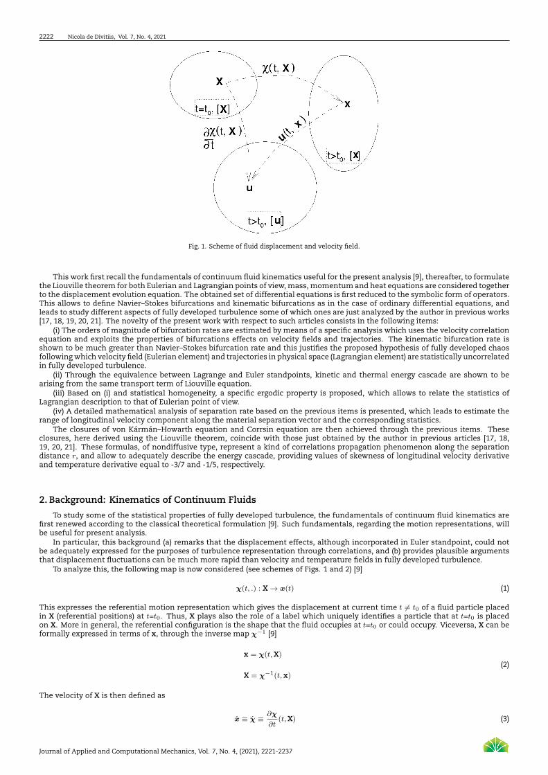
Fig. 1. Scheme of fluid displacement and velocity field.

This work first recall the fundamentals of continuum fluid kinematics useful for the present analysis [9], thereafter, to formulatethe Liouville theorem for both Eulerian and Lagrangian points of view, mass, momentum and heat equations are considered togetherto the displacement evolution equation. The obtained set of differential equations is first reduced to the symbolic form of operators.This allows to define Navier–Stokes bifurcations and kinematic bifurcations as in the case of ordinary differential equations, andleads to study different aspects of fully developed turbulence some of which ones are just analyzed by the author in previous works[17, 18, 19, 20, 21]. The novelty of the present work with respect to such articles consists in the following items:

(i) The orders of magnitude of bifurcation rates are estimated by means of a specific analysis which uses the velocity correlationequation and exploits the properties of bifurcations effects on velocity fields and trajectories. The kinematic bifurcation rate isshown to be much greater than Navier–Stokes bifurcation rate and this justifies the proposed hypothesis of fully developed chaosfollowing which velocity field (Eulerian element) and trajectories in physical space (Lagrangian element) are statistically uncorrelatedin fully developed turbulence.

(ii) Through the equivalence between Lagrange and Euler standpoints, kinetic and thermal energy cascade are shown to bearising from the same transport term of Liouville equation.

(iii) Based on (i) and statistical homogeneity, a specific ergodic property is proposed, which allows to relate the statistics ofLagrangian description to that of Eulerian point of view.

(iv) A detailed mathematical analysis of separation rate based on the previous items is presented, which leads to estimate therange of longitudinal velocity component along the material separation vector and the corresponding statistics.

The closures of von Kármán–Howarth equation and Corrsin equation are then achieved through the previous items. Theseclosures, here derived using the Liouville theorem, coincide with those just obtained by the author in previous articles [17, 18,19, 20, 21]. These formulas, of nondiffusive type, represent a kind of correlations propagation phenomenon along the separationdistance r, and allow to adequately describe the energy cascade, providing values of skewness of longitudinal velocity derivativeand temperature derivative equal to -3/7 and -1/5, respectively.

2. Background: Kinematics of Continuum Fluids

To study some of the statistical properties of fully developed turbulence, the fundamentals of continuum fluid kinematics arefirst renewed according to the classical theoretical formulation [9]. Such fundamentals, regarding the motion representations, willbe useful for present analysis.

In particular, this background (a) remarks that the displacement effects, although incorporated in Euler standpoint, could notbe adequately expressed for the purposes of turbulence representation through correlations, and (b) provides plausible argumentsthat displacement fluctuations can be much more rapid than velocity and temperature fields in fully developed turbulence.

To analyze this, the following map is now considered (see schemes of Figs. 1 and 2) [9]

χ(t, .) : X → x(t) (1)

This expresses the referential motion representation which gives the displacement at current time t = t0 of a fluid particle placedin X (referential positions) at t=t0. Thus, X plays also the role of a label which uniquely identifies a particle that at t=t0 is placedon X. More in general, the referential configuration is the shape that the fluid occupies at t=t0 or could occupy. Viceversa, X can beformally expressed in terms of x, through the inverse map χ−1 [9]

x = χ(t,X)

X = χ−1(t,x)(2)

The velocity of X is then defined as

x ≡ χ ≡∂χ

∂t(t,X) (3)

Journal of Applied and Computational Mechanics, Vol. 7, No. 4, (2021), 2221-2237

Turbulent energy cascade through equivalence of Euler and Lagrange motion descriptions and bifurcation rates 2223

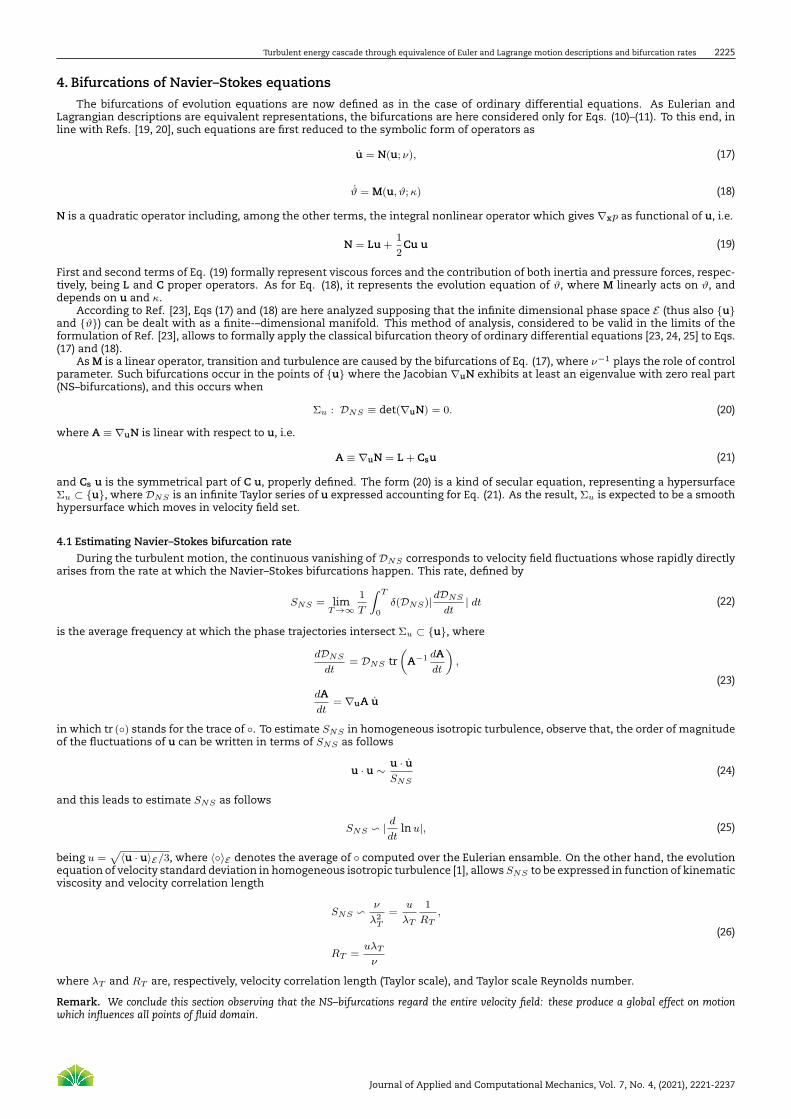
Fig. 2. Scheme of fluid displacement and temperature field.

and the temperature of X is written as

ϑm = ϑm(t,X) (4)

Equations (3)–(4) give Lagrangian or referential representation of fluid motion, being χ(t,X) and ϑm(t,X) velocity and temperaturevariations along the trajectory of X.

Following the Eulerian view point, velocity and temperature fields, u(t,x) and ϑ(t,x), are defined according to the schemes ofFigs. 1 and 2, by means of χ, ϑm and the map χ−1

u(t,x) =∂χ

∂t

(t,χ−1(t,x)

)ϑ(t,x) = ϑm

(t,χ−1(t,x)

) (5)

It is worth to remark that such Eulerian fields are not directly defined as functions of t and x. These are defined starting fromEqs. (3)–(4), as restrictions of χ(t,X) and ϑm(t,X) on the motion χ(t,X) [9]. Although the two representations are equivalent witheach other, and the Eulerian description incorporates the informations of fluid displacement through Eq. (5), unlike the referentialstandpoint, the Euler point of view does not express such informations in explicit way as χ(t,X) is implicitly incorporated in u(t,x)and ϑ(t,x). As the result, the transport effects of χ, very important in turbulence, could not be adequately represented through thesole knowledge of Eulerian fields, at least for the turbulence description in terms of correlations. Such effects are calculated throughvelocity and temperature fields as

χ(t,X) = u (t,χ(t,X)) ,

ϑm(t,X) = ϑ (t,χ(t,X))(6)

Hence, Lagrangian and Eulerian fields are defined in the functions spaces {χ(t,X)}×{ϑm(t,X)} and {u(t,x)}×{ϑ(t,x)}, respectively.At this stage of present analysis, the following should be noted

Remark. As the result of previous definitions, for an assigned motion, there are many different referential descriptions, equally valid, dependingon the referential displacement, whereas the corresponding Eulerian fields u(t,x) and ϑ(t,x) are unique [9].

Remark. Due to huge level of chaos and mixing observed in developed turbulence, according to Eqs. (5)–(6), the various fieldsχ(t,X) are expectedto be much faster than u(t,x). If u(t,x) is a slow growing function of t, then χ(t,X) could exponentially vary with respect to time. Accordingly,also ϑ(t,x) can be much slower than χ(t,X) and ϑm(t,X).

For sake of our convenience, the ratio between elemental volumes of functions spaces {χ(t,X)} × {ϑm(t,X)} and {u(t,x)} ×{ϑ(t,x)} is now calculated when χ is assigned and x = χ(t,X). This ratio is the absolute value of the determinant of the jacobian J

J =(

δ (u, ϑ)δ (χ, ϑm)

)χ

≡ I, (7)

where δ()/δ() stands for functional derivatives defined in the corresponding functions spaces, and the subscript χ here indicatesthat J is calculated for χ given and x = χ(t,X). According to Eq. (5) or (6), J identically equals the identity operator I, therefore itsdeterminant is

det J = det(

δ (u, ϑ)δ (χ, ϑm)

)χ

≡ 1, (8)

More in detail, the following functional derivatives, also computed in the same conditions(δuδχ

)χ

≡ I,(

δϑ

δϑm

)χ

≡ I (9)



correspond to identity operators, each defined in the relative function space.The considerations about the fluid temperature apply also to any passive scalar.Such background gives the starting elements of present analysis regarding some of the statistical properties of developed tur-

bulence, useful for this study.

3. Background: Evolution equations, phase space and motion descriptions

The aim of this section is to define the set of the evolution equations of fluid state variables and the corresponding phase spaces.To this end, these equations are expressed in infinite domain for both the representations, where the fluid motion is expressed withrespect to an assigned inertial frame R.

The Eulerian representation describes the motion by means of fluid properties functions of t and x. In this case, mass, momen-tum equations (Navier–Stokes equations) and heat equation are

∇x · u = 0,

u ≡∂u∂t

= −∇xu u−∇xp

ρ+ ν∇2

xu(10)

ϑ ≡∂ϑ

∂t= −u · ∇xϑ+ κ∇2

xϑ, (11)

Thus, u(t,x) and ϑ(t,x) are the fluid state variables associated with this description. According to Eq. (5), u(t,x) and ϑ(t,x) are linkedto χ(t,X), where this latter does not influence Eqs. (10) and (11), thus χ(t,X) is not a state variable and its evolution is implicitlyincluded in Eqs. (10).

For Lagrangian point of view, material properties are calculated by tracking fluid particles during the motion. In this case, theevolution equations can be written in the following way

tr((∇Xχ) (∇Xχ)−1

)= 0,

χ(1) ≡ χ ≡DuDt

≡∂u∂t

+∇xu u =1

ρ∇X · T

(12)

ϑm ≡Dϑ

Dt≡

∂ϑ

∂t+ u · ∇xϑ =

1

ρCp∇X · q (13)

χ ≡ u (t,χ) = χ(1) (14)

where T and q are stress tensor and heat flux density respectively. In this formulation, Eq. (14) is the evolution equation of fluidplacement, thus χ is a state variable of Lagrangian point of view.

The state variables for Lagrange standpoint are χ(t,X), χ(t,X) and ϑm(t,X), whereas those associated with Eulerian representa-tion are given by u(t,x) and ϑ(t,x), thus the corresponding phase spaces are E and L, being

E = {u(t,x)} × {ϑ(t,x)} ,

L = {χ(t,X)} × {χ(t,X)} × {ϑm(t,X)}(15)

Here, for sake of convenience, E and X ≡ {χ(t,X)} are called Eulerian and Lagrangian sets respectively, and the corresponding setsof solutions are Euler and Lagrange ensembles.

Observe that, according to Eq. (15) and to remarks of previous section, there is no one–to–one correspondence between the pointsof L and those of E . One point of E corresponds to infinite points of L which are all equally valid for the motion description. Thisdetermines a high level of uncertainty of displacement effects which may be unacceptable for the purposes of turbulence descriptionin terms of correlations. Here, in order to obtain a one–to–one correspondence between E and L which formally preserves all theinformations of fluid displacement, the phase space E is suitably augmented with X , introducing χ, the fluid displacement frozenat current time, whose evolution equation is

˙χ = 0 (16)

For what concerns the various quantities which appear in Eqs. (10) and (11), p=p(t,x), ν and κ=k/ρCp are pressure, kinematicviscosity and thermal diffusivity, respectively, being ρ =const, k and Cp density, fluid thermal conductivity and specific heat atconstant pressure. Here, ν and κ are supposed to be independent of temperature, thus for both the representations, momentumequations are autonomous with respect to heat equation, whereas the solutions of Eqs. (11) and (13) will depend on Eqs. (10) and (12),respectively. p is first eliminated through continuity equation, and the momentum equation is given in terms of velocity for boththe representations. Specifically, p is reduced to be a functional of u(t,x) through continuity equation. This makes the momentumequations integro–differential equations, where p exerts a nonlocal effect [22] on fluid motion.



4. Bifurcations of Navier–Stokes equations

The bifurcations of evolution equations are now defined as in the case of ordinary differential equations. As Eulerian andLagrangian descriptions are equivalent representations, the bifurcations are here considered only for Eqs. (10)–(11). To this end, inline with Refs. [19, 20], such equations are first reduced to the symbolic form of operators as

u = N(u; ν), (17)

ϑ = M(u, ϑ;κ) (18)

N is a quadratic operator including, among the other terms, the integral nonlinear operator which gives ∇xp as functional of u, i.e.

N = Lu+1

2Cu u (19)

First and second terms of Eq. (19) formally represent viscous forces and the contribution of both inertia and pressure forces, respec-tively, being L and C proper operators. As for Eq. (18), it represents the evolution equation of ϑ, where M linearly acts on ϑ, anddepends on u and κ.

According to Ref. [23], Eqs (17) and (18) are here analyzed supposing that the infinite dimensional phase space E (thus also {u}and {ϑ}) can be dealt with as a finite-–dimensional manifold. This method of analysis, considered to be valid in the limits of theformulation of Ref. [23], allows to formally apply the classical bifurcation theory of ordinary differential equations [23, 24, 25] to Eqs.(17) and (18).

As M is a linear operator, transition and turbulence are caused by the bifurcations of Eq. (17), where ν−1 plays the role of controlparameter. Such bifurcations occur in the points of {u} where the Jacobian ∇uN exhibits at least an eigenvalue with zero real part(NS–bifurcations), and this occurs when

Σu : DNS ≡ det(∇uN) = 0. (20)

where A ≡ ∇uN is linear with respect to u, i.e.

A ≡ ∇uN = L+ Csu (21)

and Cs u is the symmetrical part of C u, properly defined. The form (20) is a kind of secular equation, representing a hypersurfaceΣu ⊂ {u}, where DNS is an infinite Taylor series of u expressed accounting for Eq. (21). As the result, Σu is expected to be a smoothhypersurface which moves in velocity field set.

4.1 Estimating Navier–Stokes bifurcation rate

During the turbulent motion, the continuous vanishing of DNS corresponds to velocity field fluctuations whose rapidly directlyarises from the rate at which the Navier–Stokes bifurcations happen. This rate, defined by

SNS = limT→∞

1

T

∫ T

0δ(DNS)|

dDNS

dt| dt (22)

is the average frequency at which the phase trajectories intersect Σu ⊂ {u}, where

dDNS

dt= DNS tr

(A−1 dA

dt

),

dAdt

= ∇uA u

(23)

in which tr (◦) stands for the trace of ◦. To estimate SNS in homogeneous isotropic turbulence, observe that, the order of magnitudeof the fluctuations of u can be written in terms of SNS as follows

u · u ∼u · uSNS

(24)

and this leads to estimate SNS as follows

SNS ∽ |d

dtlnu|, (25)

being u =√

⟨u · u⟩E/3, where ⟨◦⟩E denotes the average of ◦ computed over the Eulerian ensamble. On the other hand, the evolutionequation of velocity standard deviation in homogeneous isotropic turbulence [1], allows SNS to be expressed in function of kinematicviscosity and velocity correlation length

SNS ∽ ν

λ2T

=u

λT

1

RT,

RT =uλT

ν

(26)

where λT and RT are, respectively, velocity correlation length (Taylor scale), and Taylor scale Reynolds number.

Remark. We conclude this section observing that the NS–bifurcations regard the entire velocity field: these produce a global effect on motionwhich influences all points of fluid domain.



5. Kinematic analysis

The Navier–Stokes bifurcations produce velocity and temperature fields doubling in the sense that all the properties associatedwith these fields are doubled, with particular reference to their characteristic scales ℓq and times τq , q = 1, 2,... [20] where q standsfor the number of encountered NS bifurcations when ν →0 plays the role of control parameter of Eq. (17). In detail, consider now avelocity field at a given time. When ν decreases, after the occurrence of several bifurcations, the velocity field will be representedby a function of the kind

u (t,x) = u(

t

τ1,t

τ2, ...,

t

τq;

xℓ1

,xℓ2

, ...,xℓq

), (27)

where, according to the theory [23, 26, 27, 24], the turbulence starts when q ≳ 3, 4, thereafter q diverges while ℓk and τk are continu-ously distributed.

In fully developed turbulence, the minimum of such scales, say ℓmin = min {ℓk, k = 1, 2, ...} ≡ ℓm, is identified with the conditionthat inertia and viscosity forces are locally balanced with each other, i.e.

ukℓmin

ν≈ 1,

ℓmin = uk τm,

λT = u τm.

(28)

Combining Eqs. (28) and eliminating τm, one obtains the relation

λT

ℓmin≈

u

uk≈√

RT (29)

which establishes that ℓmin and uk identify, respectively, Kolmogorov scale and the corresponding velocity. Accordingly, the trajec-tory of an arbitrary fluid particle, X, calculated following Eq. (27)

χ (t,X) = u(

t

τ1,t

τ2, ...,

t

τq;χ (t,X)

ℓ1,χ (t,X)

ℓ2, ...,

χ (t,X)ℓq

), (30)

is expected to be much more rapid and irregular with respect to velocity field fluctuations.

5.1 Trajectories bifurcations in physical space. Kinematic bifurcation rate

One point of the physical space is of bifurcation for a fluid particle trajectory if ∇xu(t,x) has at least an eigenvalue with zeroreal part, and this occurs when its determinant vanishes, i.e.

ΣK : DK ≡ det (∇xu(t,x)) = 0. (31)

Such bifurcations, here called kinematic bifurcations or trajectories bifurcations, directly cause the divergence between contiguoustrajectories in the physical space. Equation (31) defines the surface ΣK in the physical space. Due to analytical structure (27), whichincludes many arguments, ΣK is expected to be a non–smooth surface which moves in physical space.

Along one particle trajectory, the kinematic bifurcations happen with a rate, SK , defined by

SK = limT→∞

1

T

∫ T

0δ(DK)|

DDK

Dt| dt,

whereD◦Dt

=∂◦∂t

+∇x ◦ ·u =∑k

(∂◦∂tk

1

τk+

∂◦∂xk

·uℓk

),

tk =t

τk, xk =

xℓk

(32)

and

DDK

Dt= DK tr

((∇xu)−1 D∇xu

Dt

),

|∂DK

∂xk| ≈ |

∂DK

∂xh|, ∀h, k,

(33)

Specifically, SK gives the frequency at which a fluid particle trajectory intersect ΣK . Now, from Eq. (29) and taking into account thatRTmin ≈10 [28], we expect that

|∂DK

∂t| <<< |∇xDK · u| (34)

Thus, through Eq. (26), we deduce that, in fully developed turbulence, SK >>> SNS . In fact, taking into account Eqs. (32)–(34) andthat τk and ℓk are both continuously distributed, SK is of the order

SK ∽ u

ℓmin(35)



Therefore, comparing this latter with SNS , one obtains

SK

SNS∽ R

3/2T (36)

Now, the minimum value of RT in homogeneous isotropic turbulence is of the order of 10 ([28] and references therein), thus

SK

SNS>>> 1,

inf{

SK

SNS

}∽ 40 for RT ∽ 10

(37)

Following Eqs. (37)–(36), the velocity fluctuations observed along particle trajectories are much more rapid than the fluctuations ofvelocity field.

Remark. Unlike the NS–bifurcations that exert a global effect on velocity field, the kinematic bifurcations give a local influence on the particlestrajectories that only acts in close proximity of those points of physical domain which satisfy Eq. (31). On the contrary, one Navier–Stokesbifurcation, determining a doubling of velocity field, also causes a doubling of χ according to Eq. (5). Therefore, such doubling of χ is image ofthe corresponding Navier–Stokes bifurcation in the physical space. This agrees with the analysis of Ref. [29], where the energy cascade is studiedby means of a specific bifurcation analysis.

6. Statistical Analysis

The first part of this section deals with the analysis of energy cascade following the Liouville theorem. Such phenomenon ishere identified exploiting the equivalence between Eulerian and Lagrangian standpoints. The statistics of displacement, velocityand temperature fields is then studied through the previous analysis, and an ergodic property is proposed, which is based on fullydeveloped chaos and statistical homogeneity.

6.1 Equivalence of Euler and Lagrange descriptions. Liouville theorem. Energy cascade.

The statistical description of motion is given by fluid state variables distribution function, which changes following the Liouvilletheorem. For each motion description, this theorem is properly formulated through the equations of motion[30].

The distribution function associated with the Lagrangian standpoint is

PL = P (t, χ, ϑm,χ) (38)

whereas the PDF relative to Euler point of view can be obtained from Eq. (38), (7) and (16), considering the equivalence of the twodescriptions, putting x = χ(t,X) in χ and ϑm with χ = χ. This gives

PE = P (t,u, ϑ,χ) (39)

Hence, P satisfies the Liouville theorem associated with the motion equations for both the representations.In case of Euler representation, the Liouville equation arises from Eqs. (10)–(11) and (16), and reads as follows [30]

∂P

∂t+

δ

δu· (P u) +

δ

δϑ·(Pϑ)= 0 (40)

where δ/δu and δ/δϑ are functional derivatives with respect to u and ϑ respectively, being δ/δ · ◦ the divergence of ◦ in the properfunctions space. Second and third term of Eq. (40) provide the contribution of stress tensor and heat flux to ∂P/∂t, and the effectkinetic and thermal energy cascade. These latter are here expressed by H, being

H = −δ

δu· (P∇x uu)−

δ

δϑ· (P∇x ϑ · u) (41)

where first and second terms give, respectively, kinetic and thermal energy cascade contribution to rate of P .On the other hand, the Liouville equation written in the Lagrangian framework derives form Eqs. (12)–(13) and (14), and is

expressed as

∂P

∂t+

δ

δχ· (P χ) +

δ

δϑm·(Pϑm

)+

δ

δχ· (P χ) = 0 (42)

where, the terms appearing in Eq. (40) are linked to those of Eq. (42) through

δ

δχ(◦) =

δ

δu(◦)(δuδχ

)δ

δϑm(◦) =

δ

δϑ(◦)(

δϑ

δϑm

) (43)

Due to equivalence of the two motion descriptions, Eq. (42) is equivalent to Eq. (40) if x = χ(t,X) in Eq. (43). From Eq. (9) (δu/δχ)χand (δϑ/δϑm)χ are both identity operators, thus combining Eqs. (42) and (40) with Eqs. (41), one obtains H in terms of derivativeswith respect to χ, i.e.

H =δ

δχ· (P χ) (44)



As δ/δχ · (P χ) expresses the transport of P in physical space and provides both kinetic and thermal energy cascade, these latterconsist in a transport phenomenon, where the following vector

P

∇xuu

∇xϑ · u

χ

, (45)

being a solenoidal field in E × X , does not modify ∂P/∂t, in particular does not influence neither the kinetic energy rate nor thethermal energy rate.

It is worth to remark that this formulation, Eqs. (40)–(42) and (44) hold, in particular, for the temperature. More in general, suchanalysis applies, without lack of generality, to any passive scalar which exhibits diffusivity.

6.2 Statistical independence of fluid displacement and velocity field.

At this stage of the present study, we can say that, in fully developed turbulence, the fluid displacement fluctuations are indepen-dent of velocity field. To justify this, consider now the trajectory of a single particle X. Following Eq. (37), the fluctuations of χ(t,X)are much faster than velocity field. In detail, during the motion of X, the time interval between two contiguous NS–bifurcationswill contain a statistically significant number of kinematic bifurcations, expecially when RT is very high. Hence, the velocity fieldvariations are expected to be substantially irrelevant on the statistics of fluctuations of χ, where the distribution of the latter doesnot depend on the particular realization of u(t,x). Viceversa, the time variations of χ(t,X) does not influence neither u(t,x) norϑ(t,x) by definition. Thus the fluctuations of χ are supposed to be statistically independent of velocity and temperature fields andthis suggests that P (t,u, ϑ,χ) can be factorized as follows

P (t,u, ϑ,χ) = F (t,u, ϑ)Pχ(t,χ) (46)

Equations (46) and (44) represent important elements of this study. Specifically, Eq (46) represents the hypothesis of fully developedchaos of this analysis, and Eq. (44) describes the energy cascade phenomenon. Pχ, F and P are really functionals of the correspond-ing fields, defined in the functions spaces X , E and E × X , respectively. F , defining the Eulerian ensemble, provides the statistics ofvelocity and temperature fields, whereas Pχ expresses the statistics of fluid displacement (Lagrangian ensemble).

For what concerns Eq. (46), it is supported by the results of Refs. [31, 32] (and references therein), where it is observed the that:a) χ = u(t,χ) produce chaotic trajectories also for relatively simple mathematical structure of u(t,x) (also for steady fields!). b) Theflows represented by u(t,χ) stretch and fold continuously and rapidly generating a significant level of particles trajectories mixing.

6.3 Ergodic property.

Based on previous analysis, an ergodic property relating F and Pχ is here presented.Although χ(t,X) is statistically independent of the statistics of u(t,x) and ϑ(t,x), Pχ is linked to F . This arises from fully

developed chaos, statistical homogeneity and from SK/SNS >>1. To formalize this, consider now the following quantity

Υ(t,x1,x2, ...,xn) = Υ (u(t,x1), ...,u(t,xp);ϑ(t,xp+1), ..., ϑ(t,xn)) , (47)

The average of Υ calculated for x1 + χ, ..., xn + χ as follows

⟨Υχ⟩ = limT→∞

1

T

∫ T

0Υχ dt,

Υχ ≡ Υ(t,x1 + χ, ...,xn + χ),

χ = χ(t,X), ∀X ∈ {X} ,

(48)

can be also expressed in terms of Pχ and F by means of the Birkhoff ergodic theorem

⟨Υχ⟩ ≡∫E

∫X

PχFΥ(t,x1 + χ, ...,xn + χ)dXdE (49)

being∫X and

∫E functional integrals, and dX and dE the corresponding elemental volumes in the function spaces X and E . Because

of fully developed chaos and taking into account that SK/SNS >>> 1, the average of Υχ calculated over X

⟨Υχ⟩X =

∫X

PχΥ(t,x1 + χ, ...,xn + χ)dX (50)

is supposed to be independent of the specific realization of u and ϑ. This implies that ⟨Υχ⟩=⟨Υχ⟩X . On the other hand, due tohomogeneity, the average of Υχ calculated over E ,

⟨Υχ⟩E =

∫EF Υ(t,x1 + χ, ...,xn + χ) dE, (51)

does not depend on χ, therefore ⟨Υχ⟩=⟨Υχ⟩E .Hence, the link between the two ensembles consists in a kind of ergodic property where

⟨Υχ⟩E = ⟨Υχ⟩X , (52)



While Eq. (46) statistically separates Eulerian and Lagrangian ensembles, Eq. (52) gives the link between F and Pχ in case ofhomogeneous turbulence.

In particular, the statistics of velocity fluctuations along a fluid particle trajectory χ ≡ u(t,χ) is independent of F and followsPχ. In fact, such statistics can be expressed by means of F and Pχ, through the Frobenius–Perron equation

Pχ(t, χ) =

∫X

∫EF (t,u, ϑ)Pχ(t,χ)δ(χ− u(t,χ))dXdE (53)

Due to fully developed turbulence, the integral over X of Eq. (53) is expected to be independent of the particular realization of velocityfield, thus Pχ(t, χ) is estimated as

Pχ(t, χ) =

∫X

Pχ(t,χ)δ(χ− u(t,χ))dX (54)

Hence, χ(t,X) and u(t,x) are statistically independent variables related to Pχ and F , respectively.

7. Trajectories divergence in fully developed turbulence.

Due to very frequent kinematic bifurcations and fluid incompressibility, contiguous particles trajectories diverge with each other,exhibit a huge level of chaos showing a continuous relative velocity distribution. The trajectories separation evolution is given bythe following equations

χ = u(t,χ),

ξ = u(t,χ+ ξ)− u(t,χ),

(55)

where χ(t,X) and χ(t,X′) = χ(t,X)+ξ(t,X′,X) represent two trajectories associated with the particles X and X′, being ξ their relativeseparation vector. The trajectories separation rate is quantified by the radial velocity component calculated for |ξ| = r as

ξξ =ξ · ξξ · ξ

r = (u(t,χ+ ξ)− u(t,χ)) ·ξ

|ξ|(56)

Now, fluid incompressibility and kinematic bifurcations have significant implications on the interval of variations of ξξ and on thestatistics of the latter. To analyse this, consider now the representation of ξ in a proper frame and statistical isotropy

ξ =3∑

k=1

ξkek ≡3∑

k=1

ζk eφk(t)ek,

φk(0) = 0, k = 1, 2, 3

(57)

where E ≡ (e1, e2, e3) is an orthogonal unit vectors system which rotates with respect to the inertial frame R with angular velocityω depending on the local fluid motion, being ξk ≡ ζke

φk the coordinates of ξ in E. Specifically, E is chosen in such a way that e1 isthe direction of the local maximum growth rate –φ1– of ln |ξ|, whereas e2, e3 are associated with φ2 and φ3, respectively. ζk=ζk(t)and φk=φk(t), k=1, 2, 3 are slow growing functions of t. The fluid incompressibility provides

3∑k=1

φk(t) = 0, (58)

Next, the statistical isotropy, gives a condition over φk compatible with the incompressibility Eq. (58). This is analytically written as

φk(t) = φ(t) cos(β +2

3π(k − 1)), k = 1, 2, 3 (59)

As ξ is the separation vector between two fluid particles, φ(t) is a Lipschitz monotone differentiable function of t such that

∀t ∈ (−∞,∞) , 0 < φ(t) ≤ L < ∞

limt→±∞

φ(t) = ±∞,

limt→±∞

inf φ = 0,

limt→±∞

sup φ = L < +∞,

(60)

Furthermore, as e1 corresponds to the maximal rising rate direction of ln |ξ|, φ1 is maximum following Eq. (59), and this gives β = 0for φ > 0, i.e.

φ1(t) = φ(t),

φ2(t) = φ3(t) = −φ(t)

2

(61)



Now, to identify the interval of ξξ, this latter is first expressed in terms of ζk and φk as follows

ξξ =ξ · ξξ · ξ

r =

3∑k=1

(ζkζk + ζk

2φk

)e2φk

3∑k=1

ζk2e2φk

r (62)

The interval endpoints of ξξ are estimated through the limits for t → ±∞ of Eq. (62) taking into account that φ and ζk are slowgrowth functions of t, being φ also monotonic. These are

inf{ξξ

}= lim

t→−∞inf ξξ = −

L r

2,

sup{ξξ

}= lim

t→+∞sup ξξ = L r

(63)

Therefore

ξξ ∈(−M

2,M

),

M = r L

(64)

Based on previous analysis, these endpoints are independent of the particular realization of velocity field, and such limits can bealso obtained by supposing that the velocity field is frozen at a given instant.

Moreover, from Eq. (57), ξ tends to align e1, the maximum rising rate direction of ln |ξ|. For this reason, the relative velocity isusefully expressed in the following form

ξ =ξM − ξ

τ+ ω × ξ,

ξM = ξ + τ

3∑k=1

ekζkeφk

(ζk

ζk+ φk

)≈ ζ1e1eφ,

τ =1

sup φ=

1

L

(65)

Accordingly, ξξ is related to r and ξM through the following equation

ξξ −ξM

τcosα+

r

τ= 0,

where α = ξξM ,

(66)

Equation (65) is the extention of the alignment property of the classical Lyapunov vectors presented in [33] which is here appliedto finite–scale separation vectors ξ where the variations of this latter are given by φ, a monotonic Lipschitz function of t. This willcontribute to describe the turbulent energy cascade, quantifying such phenomenon.

It is worth to remark that the two radial components of velocity difference

∆ur = (u(t,x+ r)− u(t,x)) ·rr= u′

r − ur,

ξξ = (u(t,χ+ ξ)− u(t,χ)) ·ξ

r= u′

ξ − uξ

(67)

are two different quantities described by two different statistics: while ∆ur varies according to the Navier–Stokes equations, ξξchanges following the alignment property of ξ, therefore ∆ur and ξξ are represented by F and Pχ, respectively. In other words, ∆ur

is described by Eulerian ensemble, whereas ξξ follows the Lagrangian point of view. Nevertheless, in isotropic turbulence, the meansquare of ∆ur and ξξ are the same. This can be shown taking into account that the velocity correlation tensor is [1, 28]

⟨Rij⟩ ≡⟨u⊗ u′⟩

E ≡⟨uiu

′j

⟩E = u2

[−

1

2rf ′rirj +

(f +

r

2f ′)δij

](68)

and the separation vector ξ can be expressed in terms of r through its canonical representation (57)

ξ = Qr (69)

being Q a fluctuating orthogonal matrix giving the orientation of ξ with respect to R following Eq. (57), f(t, r) = ⟨uru′r⟩E/u2 is the pair

correlations of velocity longitudinal components, and u ≡√

⟨u · u⟩E/3. Therefore, accounting for isotropic hypothesis, combiningEq. (52) with Υ = u · u′ and Eqs. (68), (69) and (67), one obtains⟨

(ξξ)2⟩X

=⟨(∆ur)

2⟩E ≡ 2u2 (1− f) (70)



This gives the property that, in isotropic turbulence, the relative average kinetic energy between parts of fluid is not influencedby motion description. Although ξξ and ∆ur satisfy Eq. (70), these velocity components are distributed following very differentdistribution functions, in particular their averages are ⟨

ξξ

⟩X

> 0,

⟨∆ur⟩E = 0

(71)

where the first equation of (71) expresses that contiguous trajectories continuously diverge with each other, whereas the secondone establishes that the relative average velocity between two fixed points of space vanishes in homogeneous turbulence.

8. Statistics of separation rate.

In this section, the distribution function of ξξ, say Pξξ, is achieved by means of the previous analysis. To this purpose, we start

from the definition of ξξ

Σ : Ψ(χ, ξξ) ≡ ξξ −ξ · ξξ · ξ

r = 0 (72)

Equation (72) defines a hypersurface Σ ⊂ {X} whose measure m (Σ) is independent of ξξ due to the hypothesis of fully developedchaos. In order to obtain Pξξ

, observe that ξξ is not linked to F (t,u, ϑ) and its PDF, related to Pχ, can be expressed using Frobenius–

Perron equation [30] and alignment property (66), i.e.

Pξξ(ξξ) =

∫X

Pχ δ(Ψ(χ, ξξ)

)dχ

≡∫X

Pχ δ

(ξξ −

ξM

τcosα+

ξ

τ

)dχ

(73)

where δ stands for Dirac’s delta. Because of homogeneity, Pξξdoes not depend on x, and the idea that there are no privileged

directions in isotropic turbulence, suggests that ξξ can be uniformely distributed in its interval. To proof this, observe that theintegral of Eq. (73) can be expressed as the layer integral over Σ, i.e [34].

Pξξ(ξξ) =

∫Σ

Pχ

|∇χΨ|dΣ (74)

As Pχ, ∇χΨ and m(Σ) do not depend on ξξ, Pξξis constant in the interval of variation of ξξ, being

Pξξ(ξξ) =

2

3

1

M, if ξξ ∈

(−M

2,M

)

0 elsewhere

(75)

Another equivalent way to proof Eq. (75) exploits the statistical hypothesis of isotropy starting from

Pξξ(ξξ) =

∫X

Pχ δ

(ξξ −

ξM

τcosα+

ξ

τ

)dχ (76)

wherein ξM is considered to be given. Due to isotropy, all the directions of ξ are equiprobable, therefore the elemental probabilityPχ dX1, calculated near Σ (Ψ = 0), is relative to all those vectors ξ such that ξξM ∈ (α, α + dα), thus the corresponding elemental

volume is dX1 = {χ ⊂ X | ξξM ∈ (α, α + dα)}. This probability depends on α, being proportional to the elemental surface dS(ξ)according to Fig. 3

Pχ dX1 =dS(ξ)

4πξ2=

2πξ2 sinαdα

4πξ2= −

d cosα2

, α ∈ (0, π) , (77)

Combining Eqs. (77), (73) and (66), Pξξ(ξξ) is reduced to be an integral over cosα, where ξM is assigned. This leads to obtain Pξξ

(ξξ)

in terms of ξξ

Pξξ(ξξ) =

1

2

∫ 1

−1δ

(−ξξτ

ξM− q + cosα

)d cosα

=1

2

(H

(1−

ξξτ

ξM− q

)−H

(−1−

ξξτ

ξM− q

)),

q =r

ξM

(78)

where H indicates the Heaveside function. Therefore, ξξ is uniformely distributed in the set given by (64), according to Eq. (75).



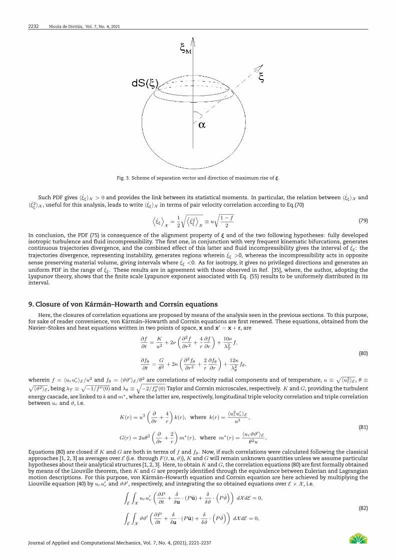
Fig. 3. Scheme of separation vector and direction of maximum rise of ξ.

Such PDF gives ⟨ξξ⟩X > 0 and provides the link between its statistical moments. In particular, the relation between ⟨ξξ⟩X and⟨ξ2ξ ⟩X , useful for this analysis, leads to write ⟨ξξ⟩X in terms of pair velocity correlation according to Eq.(70)

⟨ξξ

⟩X

=1

2

√⟨ξ2ξ

⟩X

≡ u

√1− f

2(79)

In conclusion, the PDF (75) is consequence of the alignment property of ξ and of the two following hypotheses: fully developedisotropic turbulence and fluid incompressibility. The first one, in conjunction with very frequent kinematic bifurcations, generatescontinuous trajectories divergence, and the combined effect of this latter and fluid incompressibility gives the interval of ξξ: thetrajectories divergence, representing instability, generates regions wherein ξξ >0, whereas the incompressibility acts in oppositesense preserving material volume, giving intervals where ξξ <0. As for isotropy, it gives no privileged directions and generates anuniform PDF in the range of ξξ. These results are in agreement with those observed in Ref. [35], where, the author, adopting theLyapunov theory, shows that the finite scale Lyapunov exponent associated with Eq. (55) results to be uniformely distributed in itsinterval.

9. Closure of von Kármán–Howarth and Corrsin equations

Here, the closures of correlation equations are proposed by means of the analysis seen in the previous sections. To this purpose,for sake of reader convenience, von Kármán–Howarth and Corrsin equations are first renewed. These equations, obtained from theNavier–Stokes and heat equations written in two points of space, x and x′ = x+ r, are

∂f

∂t=

K

u2+ 2ν

(∂2f

∂r2+

4

r

∂f

∂r

)+

10ν

λ2T

f,

∂fθ

∂t=

G

θ2+ 2κ

(∂2fθ

∂r2+

2

r

∂fθ

∂r

)+

12κ

λ2θ

fθ,

(80)

wherein f = ⟨uru′r⟩E/u2 and fθ = ⟨ϑϑ′⟩E/θ2 are correlations of velocity radial components and of temperature, u ≡

√⟨u2

r⟩E , θ ≡√⟨ϑ2⟩E , being λT ≡

√−1/f ′′(0) and λθ ≡

√−2/f ′′

θ (0) Taylor and Corrsin microscales, respectively. K and G, providing the turbulent

energy cascade, are linked to k and m∗, where the latter are, respectively, longitudinal triple velocity correlation and triple correlationbetween ur and ϑ, i.e.

K(r) = u3

(∂

∂r+

4

r

)k(r), where k(r) =

⟨u2ru

′r⟩E

u3,

G(r) = 2uθ2(

∂

∂r+

2

r

)m∗(r), where m∗(r) =

⟨urϑϑ′⟩Eθ2u

,

(81)

Equations (80) are closed if K and G are both in terms of f and fθ . Now, if such correlations were calculated following the classicalapproaches [1, 2, 3] as averages over E (i.e. through F (t,u, ϑ)), K and G will remain unknown quantities unless we assume particularhypotheses about their analytical structures [1, 2, 3]. Here, to obtainK andG, the correlation equations (80) are first formally obtainedby means of the Liouville theorem, then K and G are properly identified through the equivalence between Eulerian and Lagrangianmotion descriptions. For this purpose, von Kármán–Howarth equation and Corrsin equation are here achieved by multiplying theLiouville equation (40) by uru′

r and ϑϑ′, respectively, and integrating the so obtained equations over E × X , i.e.∫E

∫X

uru′r

(∂P

∂t+

δ

δu· (P u) +

δ

δϑ·(Pϑ))

dXdE = 0,

∫E

∫X

ϑϑ′(∂P

∂t+

δ

δu· (P u) +

δ

δϑ·(Pϑ))

dXdE = 0,

(82)



where second and third addends incorporate H which provides the turbulent energy cascade. The integrals of H arising from Eqs.(82) represent transport terms that do not modify the rates of kinetic and thermal energies [28, 2], and identify K and G accordingto

K = −∫E

∫X

H uru′r dXdE = −

∫E

∫X

δ

δχ·(F Pχ χ

)uru

′r dXdE,

G = −∫E

∫X

H ϑϑ′ dXdE = −∫E

∫X

δ

δχ·(F Pχ χ

)ϑϑ′ dXdE,

(83)

As for the remaining terms of Eqs. (82), these identify the other ones appearing in Eqs. (80). Integrating by parts Eqs. (83) withrespect to χ and taking into account that P=0, ∀χ ∈ ∂X , K and G are so reduced

K =

∫E

∫X

F Pχ

(∂uru′

r

∂x· χ+

∂uru′r

∂x′ · χ′)

dXdE,

G =

∫E

∫X

F Pχ

(∂ϑϑ′

∂x· χ+

∂ϑϑ′

∂x′ · χ′)

dXdE,

(84)

where F gives the average of uru′r and ϑϑ′, whereas Pχ statistically describes χ. Next, in homogeneous isotropic turbulence, the

following equations hold [1, 2, 3]

∂

∂x′ ⟨◦⟩E = −∂

∂x⟨◦⟩E =

∂

∂ξ⟨◦⟩E =

∂

∂r⟨◦⟩E

ξ

ξ(85)

where ◦ = uru′r , ϑϑ′, and ξ = χ′–χ, being x′ = χ(t,X′), x = χ(t,X), χ′ ≡ χ(t,X′), χ ≡ χ(t,X), therefore K and G read as

K = u2 ∂f

∂r

⟨ξξ

⟩X

,

G = θ2∂fθ

∂r

⟨ξξ

⟩X

,

(86)

where⟨ξξ

⟩X

is linked to f by means of Eq. (79). This leads to the following closure formulas

K(r) = u3

√1− f

2

∂f

∂r,

G(r) = uθ2√

1− f

2

∂fθ

∂r,

(87)

These equations do not exhibit second order derivatives of autocorrelations, thus Eqs. (87) are not closures of diffusive type. Theseare the result of contiguous trajectories divergence in fully developed chaos. Following Eqs. (87), the energy cascade is a sort

of propagation phenomenon along r which happens with a propagation speed⟨ξξ

⟩X

depending on r and u. The main asset of

Eqs. (87) with respect to the other closures is that such equations are not the result of phenomenological assumptions. These areachieved through the equivalence of Lagrangian and Eulerian points of view and the statistical independence of ξ and u. This latterallows to analytically express K and G separating the effects of the trajectories divergence (Lagrangian element) from velocity fieldfluctuations (Eulerian element). Due to their theoretical foundation, Eqs. (87) do not exhibit free model parameters which have tobe identified.

These closures coincide with those just obtained by the author in the previous works [17, 18, 19, 20], where the formulas areachieved using, among the other things, the finite–scale Lyapunov analysis. Here, unlike such articles, Eqs. (87) are obtained onlyusing the equivalence between Lagrangian and Eulerian motion representations, the bifurcations rates and the hypothesis of fullydeveloped chaos.

The novelty of this work with respect to [17, 18, 19, 20, 21] consists in to identify the energy cascade by means of the equivalencebetween the two motion representations, and in the estimation of ratio (NS–bifurcations rate)/(kinematic bifurcation rate) whichleads to the statistical independence of velocity field and fluid displacement. Further elements of novelty are the statistical analysisof separation rate and the proposed ergodic property, two elements which lead to Eqs. (87).

As regards the results obtained with Eqs. (87), the reader is referred to the data given in [17, 36, 18, 19, 20]. In brief, we recall thatRefs. [17, 18, 19] and [36] show that Eqs. (87) adequately describe the energy cascade phenomenon, reproducing negative values ofskewness of velocity and temperature difference

Hu3(r) ≡⟨(∆ur)3⟩

⟨(∆ur)2⟩3/2=

6k(r)

(2(1− f(r)))3/2

Hθ3(r) ≡⟨(∆ϑ)2∆ur⟩

⟨(∆ϑ)2⟩⟨(∆ur)2⟩1/2=

4m∗

2(1− fθ(r))(2(1− f(r)))1/2

(88)

and in particular

Hu3(0) = limr→0

Hu3(r) = −3

7,

Hθ3(0) = limr→0

Hθ3(r) = −1

5,

(89)

in agreement with the litarature [37, 38, 39, 40, 41, 42], the Kolmogorov law and temperature spectra in line with the theoreticalargumentation of Kolmogorov, Obukhov–Corrsin and Batchelor [43, 44, 45], with experimental results [46, 47], and with numericaldata [48, 49]. Furthermore, Ref [20] shows that the proposed closure formulas give a Kolmogorov constant of about 2, and producecorrelations self-–similarity in proper interval of r, directly caused by the continuous fluid particles trajectories divergence.



10. Results

For sake of reader convenience, some of the results just obtained in [18, 36] are here reported using the closures (87) and self–similarity expressed by f = f(r/λT ), fθ = fθ(r/λθ). The fully developed solutions of the correlation equations are obtained fordλT /dt = dλθ/dt = 0. Accordingly, von Kármán–Howarth and Corrsin equations are reduced to be ordinary differential equationswith initial conditions f(0) = 1, f ′′(0) = −1/λ2

T and fθ(0) = 1, f ′′θ (0) = −2/λ2

θ , where the apex indicates here the differentiation withrespect to r. The solutions were numerically obtained using a fourth order Runge–Kutta method with adaptive step size.

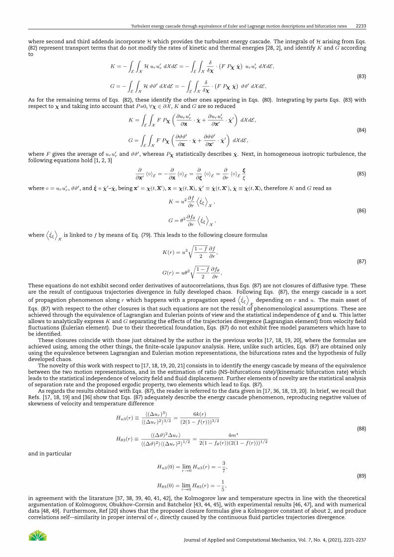
Figs. 4 and 5 show fully developed velocity correlations and the relative spectra E(κ), T (κ) numerically calculated for RT =100,200, 300, 400, 500, 600, being E(κ)

T (κ)

=1

π

∫ ∞

0

u2f(r)

K(r)

κ2r2(

sinκr

κr− cosκr

)dr (90)

where the average kinetic energy is the same for each case. From such results, the integral scale of f results to be a rising function

Fig. 4. Longitudinal velocity correlations (left) and energy spectra (right) at different Taylor scale Reynolds numbers RT =100, 200, 300, 400, 500, 600.

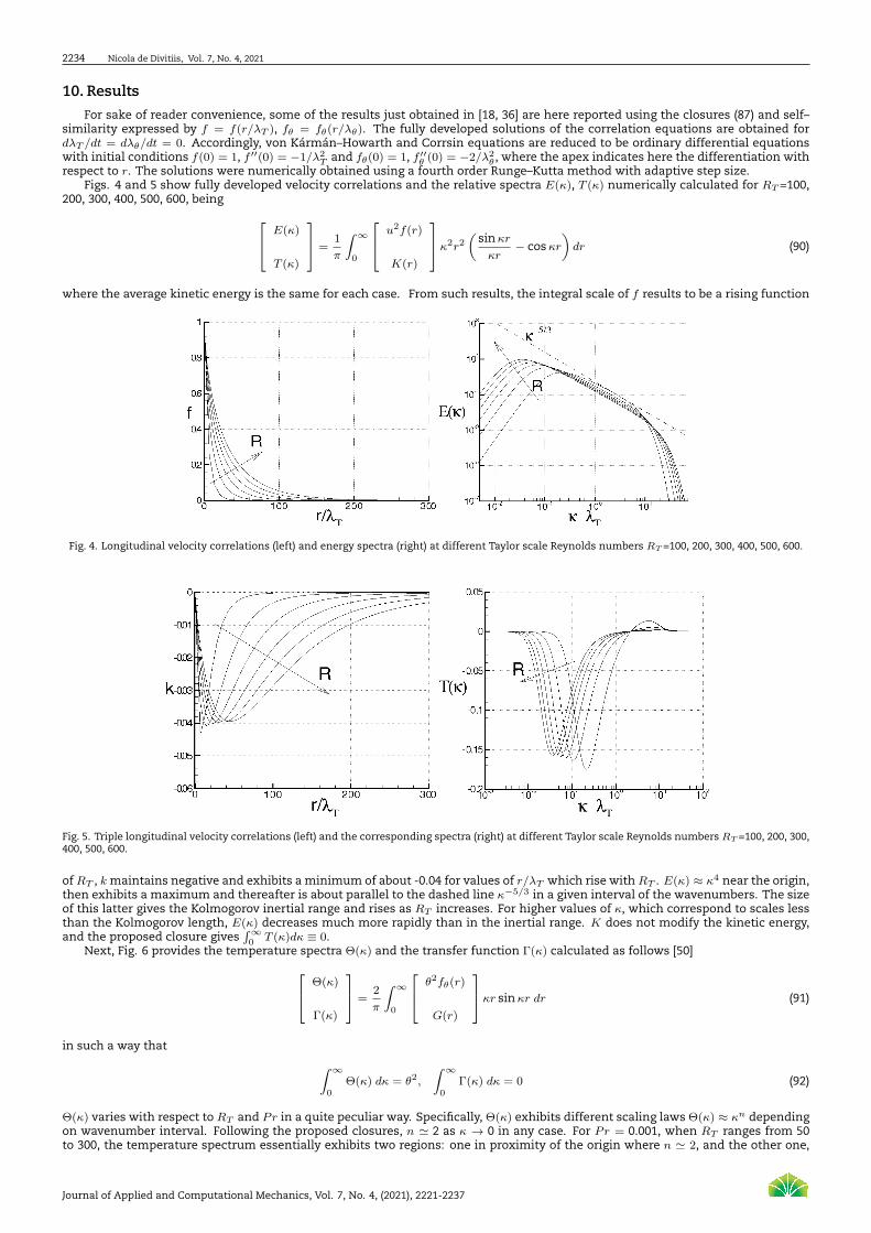
Fig. 5. Triple longitudinal velocity correlations (left) and the corresponding spectra (right) at different Taylor scale Reynolds numbers RT =100, 200, 300,400, 500, 600.

of RT , k maintains negative and exhibits a minimum of about -0.04 for values of r/λT which rise with RT . E(κ) ≈ κ4 near the origin,then exhibits a maximum and thereafter is about parallel to the dashed line κ−5/3 in a given interval of the wavenumbers. The sizeof this latter gives the Kolmogorov inertial range and rises as RT increases. For higher values of κ, which correspond to scales lessthan the Kolmogorov length, E(κ) decreases much more rapidly than in the inertial range. K does not modify the kinetic energy,and the proposed closure gives

∫∞0 T (κ)dκ ≡ 0.

Next, Fig. 6 provides the temperature spectra Θ(κ) and the transfer function Γ(κ) calculated as follows [50] Θ(κ)

Γ(κ)

=2

π

∫ ∞

0

θ2fθ(r)

G(r)

κr sinκr dr (91)

in such a way that ∫ ∞

0Θ(κ) dκ = θ2,

∫ ∞

0Γ(κ) dκ = 0 (92)

Θ(κ) varies with respect to RT and Pr in a quite peculiar way. Specifically, Θ(κ) exhibits different scaling laws Θ(κ) ≈ κn dependingon wavenumber interval. Following the proposed closures, n ≃ 2 as κ → 0 in any case. For Pr = 0.001, when RT ranges from 50to 300, the temperature spectrum essentially exhibits two regions: one in proximity of the origin where n ≃ 2, and the other one,



Fig. 6. Spectra for Pr= 10−3, 10−2, 0.1, 1.0 and 10, at different Reynolds numbers. Top: kinetic energy spectrum E(κ) (dashed line) and temperaturespectra Θ(κ) (solid lines). Bottom: velocity transfer function T (κ) (dashed line) and temperature transfer function Γ(κ) (solid line).

at higher values of κ, where −17/3 < n < −11/3, (value very close to −13/3). The value of n ≈ −13/3, here obtained in an intervalaround to r ≈1, is in between the exponent proposed by [44] (−17/3) and the value determined by [48] (−11/3) by means of numericalsimulations. Increasing κ, n significantly diminishes, and Θ(κ) does not show scaling law. When Pr =0.01, an interval near r ≈ 1where −17/3 < n < −13/3 appears, and this agrees with [44]. For Pr =0.1, the previous scaling law vanishes, whereas for RT = 50and 100, n changes with κ, and Θ(κ) does not express clear scaling laws. When RT = 300, the birth of a small region is observed,where n ≈ −5/3 has an inflection point. For Pr = 0.7 and 1, with RT = 300, the width of this region is increased, whereas at Pr =10, and RT = 300, two regions are observed: one interval where n has a local minimum with n ≃ −5/3, and the other one where nexhibits a relative maximum, with n ≃ −1. For larger κ, n diminishes and the scaling laws disappear. The presence of the scalinglaw n ≃ −5/3 agrees with the theoretical arguments of [3, 45] (see also [47, 49] and references therein). Figure 6 also reports (on thebottom) the spectra Γ(κ) (solid lines) and T (κ) (dashed lines) which describe the energy cascade mechanism.

We conclude this study by observing the limits of the proposed closures. These limits directly derive from the hypotheses underwhich Eqs. (87) are obtained: Eqs. (87) are valid only in regime of fully developed chaos where the turbulence exhibit homogene-ity and isotropy. Otherwise, during the transition through intermediate stages of turbulence, or in more complex situations withparticular boundary conditions, for instance in the presence of wall, Eqs. (87) cannot be applied. In this regard, note that, with-out the hypotheses of statistical isotropy and homogeneity, the energy cascade is however identifiable through H and Liouvilletheorem, whereas the determination of separation rate statistics, closures of correlation equations and other correlations such aspressure–velocity, remains a very difficult task depending on the particular problem.

11. Conclusion

The energy cascade in isotropic homogeneous turbulence is studied through Euler and Lagrange points of view using the bi-furcation rates. The order of magnitude of such rates justifies that velocity field (Eulerian element) and trajectories (Lagrangianelement) are statistically uncorrelated, and the turbulent energy cascade is identified by exploiting the equivalence of Eulerian andLagrangian motion descriptions through Liouville theorem. A specific ergodic property is then proposed, which relates the statisticsof both the descriptions, and a detailed analysis of separation rate is presented, which leads to the statistics of radial velocity com-ponent. Finally, the closures of von Kármán–Howarth equation and Corrsin equation are determined. These coincide with those justdetermined by the author in previous articles [17, 18, 19, 20, 21], corroborating the previous works. These formulas, of nondiffusivenature, allow to adequately describe the phenomenon of energy cascade.

Acknowledgments

This work was partially supported by the Italian Ministry for the Universities and Scientific and Technological Research (MIUR).

Conflict of Interest

The author declared no potential conflicts of interest with respect to the research, authorship and publication of this article.

Funding

The author received no financial support for the research, authorship and publication of this article.



References[1] von Kármán, T., Howarth, L., On the Statistical Theory of Isotropic Turbulence., Proc. Roy. Soc. A, 164, 14, 192, (1938).[2] Corrsin S., The Decay of Isotropic Temperature Fluctuations in an Isotropic Turbulence, Journal of Aeronautical Science, 18, pp. 417–423, no. 12,

(1951).[3] Corrsin S., On the Spectrum of Isotropic Temperature Fluctuations in an Isotropic Turbulence, Journal of Applied Physics, 22, pp. 469–473, no. 4,

(1951), DOI: 10.1063/1.1699986.[4] Hasselmann K., Zur Deutung der dreifachen Geschwindigkeitskorrelationen der isotropen Turbulenz, Dtsch. Hydrogr. Z, 11, 5, 207-217, (1958).[5] Millionshtchikov M., Isotropic turbulence in the field of turbulent viscosity, JETP Lett., 8, 406–411, (1969).[6] Oberlack M., Peters N., Closure of the two-point correlation equation as a basis for Reynolds stress models, Appl. Sci. Res., 51, 533–539, (1993).[7] Baev M. K. & Chernykh G. G., On Corrsin equation closure, Journal of Engineering Thermophysics, 19, pp. 154–169, no. 3, (2010), DOI:

10.1134/S1810232810030069[8] Domaradzki J. A., Mellor G. L. , A simple turbulence closure hypothesis for the triple-velocity correlation functions in homogeneous isotropic

turbulence, Jour. of Fluid Mech., 140, 45–61, (1984).[9] Truesdell, C. A First Course in Rational Continuum Mechanics, Academic, New York, (1977).

[10] George W. K., A theory for the self-preservation of temperature fluctuations in isotropic turbulence. Technical Report 117, Turbulence ResearchLaboratory, January (1988).

[11] George W. K., ”Self-preservation of temperature fluctuations in isotropic turbulence,” in Studies in Turbulence, Springer, Berlin, (1992).[12] Antonia R. A., Smalley R. J., Zhou T., Anselmet F., Danaila L., Similarity solution of temperature structure functions in decaying homogeneous

isotropic turbulence, Phys. Rev. E, 69, 016305, (2004), DOI: 10.1103/PhysRevE.69.016305[13] Onufriev, A., On a model equation for probability density in semi-empirical turbulence transfer theory. In: The Notes on Turbulence. Nauka,

Moscow, (1994)[14] Grebenev V.N., Oberlack M. A Chorin-Type Formula for Solutions to a Closure Model for the von Kármán-Howarth Equation, J. Nonlinear Math.

Phys., 12, 1, 1–9, (2005)[15] Grebenev V.N., Oberlack M. A Geometric Interpretation of the Second-Order Structure Function Arising in Turbulence, Mathematical Physics,

Analysis and Geometry, 12, 1, 1-18, (2009)[16] Thiesset F., Antonia R. A., Danaila L., and Djenidi L. , Kármán–Howarth closure equation on the basis of a universal eddy viscosity, Phys. Rev. E,

88, 011003(R), (2013), doi: 10.1103/PhysRevE.88.011003.[17] de Divitiis, N., Lyapunov Analysis for Fully Developed Homogeneous Isotropic Turbulence, Theoretical and Computational Fluid Dynamics, (2011),

DOI: 10.1007/s00162-010-0211-9.[18] de Divitiis, N., Finite Scale Lyapunov Analysis of Temperature Fluctuations in Homogeneous Isotropic Turbulence, Appl. Math. Modell., (2014),

DOI: 10.1016/j.apm.2014.04.016.[19] de Divitiis N., von Kármán–Howarth and Corrsin equations closure based on Lagrangian description of the fluid motion, Annals of Physics, vol.

368, May 2016, Pages 296-309, (2016), DOI: 10.1016/j.aop.2016.02.010.[20] de Divitiis N., Statistical Lyapunov theory based on bifurcation analysis of energy cascade in isotropic homogeneous turbulence: a physical–

mathematical review, Entropy, vol. 21, issue 5, p. 520, 2019, DOI: 10.3390/e21050520.[21] de Divitiis N., von Kármán–Howarth and Corrsin equations closures through Liouville theorem, Results in Physics, vol. 2020,

doi:10.1016/j.rinp.2020.102979.[22] Tsinober, A. An Informal Conceptual Introduction to Turbulence: Second Edition of An Informal Introduction to Turbulence, Springer Science & Business

Media, (2009).[23] Ruelle, D., Takens, F., Commun. Math Phys. 20, 167, (1971).[24] Eckmann, J.P., Roads to turbulence in dissipative dynamical systems Rev. Mod. Phys. 53, 643–654, (1981).[25] Guckenheimer, J., Holmes, P., Nonlinear Oscillations, Dynamical Systems, and Bifurcations of Vector Fields. Springer, (1990).[26] Feigenbaum, M. J., J. Stat. Phys. 19, (1978).[27] Pomeau, Y., Manneville, P., Commun Math. Phys. 74, 189, (1980).[28] Batchelor, G.K., The Theory of Homogeneous Turbulence. Cambridge University Press, Cambridge, (1953).[29] de Divitiis N., Bifurcations analysis of turbulent energy cascade, Annals of Physics, (2015), DOI: 10.1016/j.aop.2015.01.017.[30] Nicolis, G., Introduction to nonlinear science, Cambridge University Press, (1995).[31] Ottino, J. M. The kinematics of mixing: stretching, chaos, and transport, Cambridge Texts in Applied Mathematics, New York, (1989).[32] Ottino, J. M., Mixing, Chaotic Advection, and Turbulence., Annu. Rev. Fluid Mech. 22, 207–253, (1990).[33] Ott E., Chaos in Dynamical Systems, Cambridge University Press, (2002).[34] Federer, H., Geometric Measure Theory, Springer–Verlag, 1969.[35] de Divitiis N., Statistics of finite scale local Lyapunov exponents in fully developed homogeneous isotropic turbulence, Advances in Mathematical

Physics, vol. 2018, Article ID 2365602, 12 pages, (2018), https://doi.org/10.1155/2018/2365602.[36] de Divitiis, N., Self-Similarity in Fully Developed Homogeneous Isotropic Turbulence Using the Lyapunov Analysis, Theoretical and Computational

Fluid Dynamics, (2012), DOI: 10.1007/s00162-010-0213-7.[37] Chen S., Doolen G.D., Kraichnan R.H., She Z-S., On statistical correlations between velocity increments and locally averaged dissipation in

homogeneous turbulence, Phys. Fluids A, 5, pp. 458–463, (1992).[38] Orszag S.A., Patterson G.S., Numerical simulation of three-dimensional homogeneous isotropic turbulence., Phys. Rev. Lett., 28, 76–79, (1972).[39] Panda R., Sonnad V., Clementi E. Orszag S.A., Yakhot V., Turbulence in a randomly stirred fluid, Phys. Fluids A, 1(6), 1045–1053, (1989).[40] Anderson R., Meneveau C., Effects of the similarity model in finite-difference LES of isotropic turbulence using a lagrangian dynamic mixed

model, Flow Turbul. Combust., 62, pp. 201–225, (1999).[41] Carati D., Ghosal S., Moin P., On the representation of backscatter in dynamic localization models, Phys. Fluids, 7(3), pp. 606–616, (1995).[42] Kang H.S., Chester S., Meneveau C. , Decaying turbulence in an active–gridgenerated flow and comparisons with large–eddy simulation., J. Fluid

Mech. 480, pp. 129–160, (2003).[43] Batchelor, G. K., Small-scale variation of convected quantities like temperature in turbulent fluid. Part 1. General discussion and the case of

small conductivity, Journal of Fluid Mechanics, 5, (1959), pp. 113–133[44] Batchelor G. K., Howells I. D., Townsend A. A., Small-scale variation of convected quantities like temperature in turbulent fluid. Part 2. The

case of large conductivity, Journal of Fluid Mechanics, 5, (1959), pp. 134–139[45] Obukhov, A. M., The structure of the temperature field in a turbulent flow. Dokl. Akad. Nauk., CCCP, 39, (1949), pp. 391.[46] Gibson, C. H., Schwarz W. H., The Universal Equilibrium Spectra of Turbulent Velocity and Scalar Fields, Journal of Fluid Mechanics, 16, (1963), pp.

365–384[47] Mydlarski, L., Warhaft, Z., Passive scalar statistics in high-Péclet-number grid turbulence, Journal of Fluid Mechanics, 358, (1998), pp. 135–175[48] Chasnov, J., Canuto V. M., Rogallo R. S., Turbulence spectrum of strongly conductive temperature field in a rapidly stirred fluid. Phys. Fluids A,

1, pp. 1698-1700, (1989), doi:10.1063/1.857535.[49] Donzis D. A., Sreenivasan K. R., Yeung P. K., The Batchelor Spectrum for Mixing of Passive Scalars in Isotropic Turbulence, Flow, Turbulence and

Combustion, 85, pp. 549–566, no. 3–4, (2010), DOI: 10.1007/s10494-010-9271-6[50] Ogura, Y., Temperature Fluctuations in an Isotropic Turbulent Flow, Journal of Meteorology, 15, (1958), pp. 539-–546

ORCID iD

Nicola de Divitiis https://orcid.org/0000-0002-9788-6113

© 2021 Shahid Chamran University of Ahvaz, Ahvaz, Iran. This article is an open access article distributed under theterms and conditions of the Creative Commons Attribution-NonCommercial 4.0 International (CC BY-NC 4.0 license)(http://creativecommons.org/licenses/by-nc/4.0/)



How to cite this article: Nicola de Divitiis. Turbulent energy cascade through equivalence of Euler and Lagrange motion de-scriptions and bifurcation rates , J. Appl. Comput. Mech., 7(4), 2021, 2221-2237. https://doi.org/10.22055/JACM.2021.38082.3149

Publisher’s Note Shahid Chamran University of Ahvaz remains neutral with regard to jurisdictional claims in published maps andinstitutional affiliations.


Turbulent energy cascade through equivalence of Euler and ...

Documents

Transcript of Turbulent energy cascade through equivalence of Euler and ...