3D Euler about a 2D Symmetry Plane

Miguel D. Bustamante1, ∗ and Robert M. Kerr1

1Mathematics Institute, University of Warwick, Coventry CV4 7AL, United Kingdom

Initial results from new calculations of interacting anti-parallel Euler vortices are presented withthe objective of understanding the origins of singular scaling presented by Kerr (1993) and the lackthereof by Hou and Li (2006). Core profiles designed to reproduce the two results are presented, newmore robust analysis is proposed, and new criteria for when calculations should be terminated areintroduced and compared with classical resolution studies and spectral convergence tests. Most ofthe analysis is on a 512×128×2048 mesh, with new analysis on a just completed 1024×256×2048used to confirm trends. One might hypothesize that there is a finite-time singularity with enstrophygrowth like Ω ∼ (Tc− t)−γΩ and vorticity growth like ‖ω‖∞ ∼ (Tc− t)−γ . The new analysis wouldthen support γΩ ≈ 1/2 and γ > 1. These represent modifications of the conclusions of Kerr (1993).Issues that might arise at higher resolution are discussed.

PACS numbers: 47.10.A-, 47.11.Kb, 47.15.kiKeywords: Euler equations, fluid singularities, vortex dynamics.

I. INTRODUCTION

One definition of solving Euler’s three-dimension in-compressible equations [1] is determining whether or notthey dynamically generate a finite-time singularity if theinitial conditions are smooth, in a bounded domain andhave finite energy. The primary analytic constraint thatmust be satisfied [2] is:∫ T

0

‖ω‖∞ dt→∞ (1)

where ‖ω‖∞ is the maximum of vorticity over all space.To date, Kerr (1993) [3] remains the only fully three-dimensional simulation of Euler’s equations with evi-dence for a singularity consistent with this and relatedconstraints [4]. Growth of the enstrophy production andstretching along the vorticity, plus collapse of positions,supported this claim [3]. Additional weaker evidence re-lated to blow-up in velocity and collapsing scaling func-tions was presented later [5].

There is only weak numerical evidence supportingthese claims [6, 7]. In a recent paper, as described inone of the invited talks of this symposium, Hou and Li(2006) [8] found evidence that the above scenario failedat late times.

This contribution will first comment on four issuesraised at the symposium, then present preliminary newresults. The four issues are:

• How should spurious high-wavenumber energy inspectral methods be suppressed?

• What criteria should be used to determine whennumerical errors are substantial?

• What effect do the initial conditions have on singu-lar trends? A cleaner initial condition is proposed.

∗Electronic address: mig busta@yahoo.com

• We introduce a new approach for determiningwhether there is singular behavior of the primaryproperties and the associated scaling. This is ap-plied to both new and old data.

All calculations will be in the following domain: Lx ×Ly × Lz = 4π × 4π × 2π with free-slip symmetries iny and z and periodic in x with up to nx × ny × nz =1024× 256× 2048 mesh points. Using these symmetriesonly one-half of one of the anti-parallel vortices needs tobe simulated.

The “symmetry” plane will be defined as xz free-slipsymmetry through the maximum perturbation of the ini-tial vortices and the “dividing” plane will be defined asthe xy free-slip symmetry between the vortices.

II. HOW SHOULD SPURIOUSHIGH-WAVENUMBER ENERGY IN SPECTRAL

METHODS BE SUPPRESSED?

A generic difficulty in applying spectral methods to lo-calized physical space phenomena is the accumulation ofspurious high-wavenumber energy that leads to numeri-cal errors.

What is the best approach for eliminating these spuri-ous modes? We have compared the old-fashioned 2/3rdsdealiasing versus the recently proposed 36th-power hy-perviscous filter [8, 11]. Detailed tests to be described ina later paper show that the latter is better in the sensethat for several quantities, such as the peak vorticity,lower resolution calculations follow the high resolutioncases longer. But a combination of the two approachesworks even better, and that is what is used here.

Still, caution is required for any of these approachesas the hyperviscosity can dissipate small structures suchas the anomalous negative vorticity in the squared-offprofile below. Surprisingly the 36th-order hyperviscositydoes not appear to produce the ghost vortices that are aknown artifact of lower-order schemes.

arX

iv:0

802.

3369

v1 [

phys

ics.

flu-

dyn]

22

Feb

2008

2

III. WHAT CRITERIA SHOULD BE USED TODETERMINE WHEN NUMERICAL ERRORS

ARE SUBSTANTIAL?

There are traditionally two approaches to this prob-lem, one emphasizing local quantities such as ‖ω‖∞ , andthe other emphasizing global quantities such as the meansquare vorticity or enstrophy. We use both.

1. Local quantities and resolution

To determine local resolution it is important to checkthe convergence of local quantities such as:

• The maximum of vorticity ‖ω‖∞ . The location of‖ω‖∞ will be defined as x∞.

• The local stretching of vorticity

α = ωieijωj (2)

where ω = ω/|ω| and eij = 12 (ui,j + uj,i).

Following earlier work [3, 8], we use the criteria thatx∞ cannot be closer than 6 mesh points from the dividingplane.

2. Integral quantities

Examples of integral quantities we could monitor are:energy, circulation (which are in principle conserved), en-strophy and helicity (which are in principle changing).

i) Energy is robustly conserved by spectral methodseven when under-resolved and therefore is not auseful test. Convergence of the energy spectrum[8] is only a partial test because it neglects phaseerrors.

ii) Circulation in the upper half of the symmetry plane(i.e., the z > 0 half of the xz-plane, which isperpendicular to the primary direction of vortic-ity y) is conserved. Circulation in the equivalenthalf of the dividing plane is also conserved. In allof the initial conditions considered here, it is ini-tially zero and ideally should remain so. There-fore, the circulations of the symmetry and divid-ing planes, σy =

∫z>0

ωy(x, 0, z, t)dx dz and σz =∫y>0

ωz(x, y, 0, t)dx dy were monitored.

We have found that serious depletion of σy is con-trolled by nz and the time this begins is indepen-dent of the high-wavenumber filter. Once nz is set,by convergence of ‖ω‖∞ , we find that there is goodconvergence if nx = nz/2 and ny = nz/4. A laterpaper will provide more details on these conver-gence tests. We will violate the condition on ny atlate times due to current memory restrictions.

Without the circulation test, it is difficult to drawconclusions about the late times in Hou and Li(2006) [8] where they claim to see divergence fromthe scaling of Kerr (1993) [3].

iii) Enstrophy Ω grows in time, so one test is to checkhow it is balanced by its production Ωp, which wedetermine directly. The enstrophy and its produc-tion are

Ω =∫dV ω2 , Ωp = 2

∫dV ωieijωj . (3)

iv) Helicity grows within the quadrant simulated (notover the full anti-parallel geometry), but its pro-duction is determined by pressure which has notbeen calculated.

IV. WHAT IS THE EFFECT OF THE INITIALCONDITIONS ON THE POTENTIALLY

SINGULAR BEHAVIOR?

A. Earlier descriptions

Because ambiguities in the earlier description of theinitial condition of [3] led to differences in the initial con-dition of Hou and Li (2006) [8], the community needs aclear description of a reproducible, clean initial conditionthat yields the trends of Kerr (1993) [3]. Ideally, we wantan initial condition whose vorticity is purely positive inthe upper half of the symmetry plane, which followingKelvin’s theorem will remain positive for all subsequenttimes. These steps were used [3] to massage the vortexprofile in order to achieve this:

1) The first step in creating the initial profile of thevorticity core is to use an explicit function wherethe value and all derivatives went smoothly to zeroat a given radius. See references in [3] for earlierwork that had used a similar profile. To this, alocalized perturbation in its position in x was given[9].

2) The second step is to remove high-wavenumbernoise by applying a symmetric high-wavenumberfilter of the form: exp(−a(k2

x + k2y + k2

z)2). Kerr(1992) [10] showed the undesirable side-effects ifthis is not done. However, it has become apparentthat the high-wavenumber filter is not sufficient.

B. Effect of a negative region

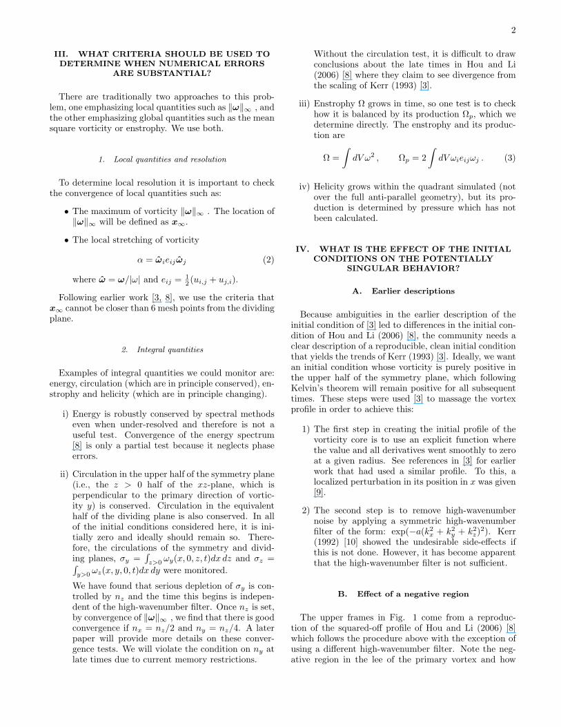
The upper frames in Fig. 1 come from a reproduc-tion of the squared-off profile of Hou and Li (2006) [8]which follows the procedure above with the exception ofusing a different high-wavenumber filter. Note the neg-ative region in the lee of the primary vortex and how

3

FIG. 1: ωy in the symmetry plane from two initial conditions for t = 0 and for early times with roughly the same growth inmax(ωy) in the symmetry plane. The first squared profile is nearly the same as used by Hou and Li (2006) [8] using step 1) withmax(ωy) = 0.49 in the symmetry plane (over all space ‖ω‖∞ = max(|ω|) = .67) and for step 2) a squared-off high-wavenumberfilter (exp(−a(k4

x + k4y + k4

z)). Note the large negative vorticity in the lee (right) of the primary vortex as in Hou and Li (2006)[8] (Fig. 2) and how this is entrained underneath the primary vortex at t = 6, whereupon the hyperviscous filter will dissipateit. In the new profile step 3 is included: adding positive ωy(z). In this case max(ωy) = 0.83 in the symmetry plane and overall space ‖ω‖∞ = 1.05. There is no anomalous negative vorticity and numerical solutions require less resolution.

this is sucked underneath the primary vortex at t = 6.The t = 6 frame represents the vortices simulated withthe 36th-order hyperviscosity [8, 11]. For t > 6 this sec-ondary vortex is dissipated by the hyperviscosity and cir-culation is dissipated, meaning these calculations are notfaithfully representing the Euler equations. Without thehyperviscosity, numerical noise would dominate as an ex-tra boundary layer needs to be resolved.

C. Final step 3) for purely positive

What is apparently missing from the previous descrip-tion [3] is the addition of a mean shear designed to removethe final negative regions in the symmetry plane. Thiswas achieved before [3] as part of an interpolation pro-cedure from a uniform mesh to a Chebyshev mesh. Hereit is imposed. Details will appear in a full paper. Ini-tial vorticity in the symmetry plane and a slightly latertime (t = 4.38) are shown. This is the initial conditionfor which we have now done up to 1024 × 256 × 2048calculations to assess the scaling proposed earlier [3].

V. A NEW APPROACH FOR DETERMININGWHETHER THERE IS SINGULAR BEHAVIOROF THE PRIMARY PROPERTIES AND THE

ASSOCIATED SCALING.

Once reliable data (according to the criteria discussedabove) has been obtained, it is common to interpret it

in terms of power laws and other simple formulae. Forexample, assume that

f(t) ∼ C/(Tc − t)γ . (4)

To properly find all three free parameters (C, Tc and γ)to a set of points requires a minimization procedure.

Kerr (1993) avoided this by assuming particularly sim-ple values for γ for several quantities. In particularγ = 1 was assumed for ‖ω‖∞ , for the maximum of thestretching of the vorticity (2) in the symmetry plane:max(α)|y=0, and for the enstrophy production (3). Thisprocedure was extended to the velocity by assuming thatγu = 1/2 for sup(|u|) [5].

While fits with these assumptions gave consistent re-sults for the singular time Tc, this consistency existedonly at late times when resolution was becoming ques-tionable. Analysis of this data by two new methods hasshown that the lack of scaling at earlier times is due inpart to some of the more restrictive assumptions thatwere made.

A. Three-parameter fitting

Our first indication that earlier assumptions [3, 5]might be incorrect was obtained by allowing γ to be free.The three parameters (C, Tc and γ) were then obtainedas follows: by minimizing the sum of squares of the dif-ferences between the logarithm of the data and the loga-rithm of the fit function, with respect to C and γ, allows

4

one to solve for these two parameters in terms of Tc. Thenthe sum of squares is further minimized with respect toTc to obtain all three parameters.

This analysis was applied to ‖ω‖∞ and Ωp, the enstro-phy production, both of which previously were assumedto have 1/(Tc − t) behavior.

It was immediately observed that

• The fitting parameters depended upon the range oftimes chosen.

• γ in each case was consistently greater than 1.

This would not be inconsistent with known bounds.Recall if power law behavior is expected for ‖ω‖∞ , (1)only requires that γ ≥ 1.

B. Logarithmic time derivatives of enstrophy and‖ω‖∞ : instantaneous two-parameter fitting

The original analysis would be possible if there is asecondary quantity which must go as 1/(Tc − t) if theprimary quantity obeys the power law 1/(Tc − t)γ . Anexample of a secondary quantity of that sort is the log-arithmic time derivative of the primary quantity, whichcan be computed if we know independently the quantityf(t) and its time derivative f(t).

Therefore we propose a new approach to inferring asingular time and identifying the scaling behaviour:

• Find a quantity f(t) whose growth and the growthof its time-derivative can be determined directly.Consider the new function:

g(t) =(d

dtlog f(t)

)−1

=f.f

=1γ

(Tc − t) . (5)

Note that the parameter C drops out and the func-tion is linear, so we can predict instantaneous val-ues of γ and Tc by fitting this new function usingadjacent points in time.

• Calculating in this manner, using nearest neigh-bours in time, yields instantaneous predicted sin-gular times Tc(t) and power laws γ(t). These in-stantaneous parameters will generically depend ontime.

• See if these converge or relax (as time increases).

Pairs of quantities to which this procedure can be ap-plied are:

• ‖ω‖∞ and its logarithmic time derivative α∞ (localstretching at the point x∞).

• Enstrophy Ω and its production Ωp (3) where weassume that

Ω ∼ CΩ

(Tc − t)γΩ. (6)

• Helicity in the simulated quadrant of space and itsproduction.

This approach is applied to enstrophy and its pro-duction on our highest resolution simulations. Becauseenstrophy and its production are global quantities theyconverge numerically longer (to t = 11.25) than ‖ω‖∞ ,for which x∞ is less than 6 mesh points from the divid-ing plane for t > 10. Running estimates for Tc and γΩ

are shown in Fig. 2. For the new data (upper frames),the latest data point gives an estimate Tc ≈ 13.16 andγΩ ≈ 0.47. The bottom frames show the same analy-sis applied to the data used by Kerr (1993) [3]. Nearlyidentical power laws are obtained (γΩ ≈ 0.50), with apredicted singular time Tc ≈ 19.69, greater than in Kerr(1993).

One advantage of finding running estimates of Tc isthat it can be used to identify cases that are not sin-gular, or would take an unusually long time to becomesingular. This is done by looking at the instantaneousestimated value of Tc. If Tc continues to increase withtime, then there is evidence for regularity. In both thenew calculations and for the data from Kerr (1993), even-tually the estimated Tc decreases and relaxes to a finitevalue. It is quite possible that there is a large pre-factorin front of the power law, which the time dependence ofthe estimated γΩ and CΩ might be able to shed light on.

This approach assumes smooth values for both quanti-ties in a pair. Unfortunately, we have found that because‖ω‖∞ sits on a steep gradient of α, values of α∞ on thelower resolution mesh were not smooth enough in timeto perform this analysis. The analysis will be attemptedon the higher resolution (‖ω‖∞ ,α∞) data when that ad-ditional analysis of the new data sets is available.

C. Convergence studies: Is the evidence forsingularity conclusive?

Further tests at higher resolution are needed to supportthe singular trends seen here. Both current cases (oldand new data) could be reliably integrated up to timest ≈ Tc − 2.75. This would only be the beginning of theasymptotic regime of the potentially singular solution, asis suggested by the late-time behavior of the curves forthe predicted singular time Tc in Fig. 2. New calculationsin progress should go beyond that barrier and help testthe validity of the hypothesis of finite-time singularity.

In this subsection we show resolution studies with nzfixed to give a flavor of what will be shown in the nextpaper (we have also made resolution checks with fixednx or ny and varying the other two, not shown here).The resolution study is a classical tool to validate andfind reliability times for the numerical results. Anothernow widely accepted study that we present is a spectralconvergence test (Sulem et al., 1983 [12]) used recentlyby Cichowlas and Brachet (2004) (see [13] and referencestherein), where the exponential decay of the energy spec-trum as a function of the wavenumber is employed to give

5

5 6 7 8 9 10 11t

6

8

10

12

Tc

5 6 7 8 9 10 11t

0.2

0.3

0.4

0.5

ΓW

8 10 12 14 16 18t7.5

10

12.5

15

17.5

20

22.5

25

Tc

8 10 12 14 16 18t

0.4

0.6

0.8

1

1.2

1.4

ΓW

FIG. 2: Upper frames: Resolution study of the predicted singular time Tc and the predicted exponent γΩ in the power-lawbehavior of the total enstrophy Ω using the new data at resolutions: 512× 64× 2048 (dashed), 512× 128× 2048 (dotted) and1024× 256× 2048 (solid).Lower frames: Predicted Tc and γΩ for the Kerr (1993) data at the highest resolution (solid). Dashed lines denote gaps in data.In the graphs for the predicted Tc, the dash-dotted diagonal lines denote the Tc = t singularity asymptote.

a criteria for the reliability time. Finally we complementthe above classical tests with our newly proposed tests ofreliability: conservation of circulation through the sym-metry plane and conservation of circulation through thedividing plane.

We consider first the behavior of local quantities, inthe sense of Section III. Figure 3 (top) is a resolutionstudy of the time dependence of the maximum vorticity;the bottom figure is a t = 10 anisotropic energy spec-trum E(kx, t), defined by averaging the Fourier transformu(k′, t) of the velocity field on flat duplicated sheets ofwidth ∆kx = 1,

E(kx, t) =12

∑kx−∆kx/2<|k′

x|<kx+∆kx/2

|u(k′, t)|2 .

Following [13], we fit: logE(kx) = C − n log(kx)− 2δ kx(solid line in the figure). The test consists in monitoringthe parameter δ as a function of time. The idea is thatδ, being the width in the complex plane of the analyt-icity strip of the velocity field, should always be numer-ically resolved, at least by the mesh size. Another way

to look at this condition is to ask that the contributionof the exponential term to the change of logE(kx) fromthe largest to the smallest scale allowed by the numer-ical resolution, be greater than a prescribed factor. Inmore explicit terms, we can only fully trust the simula-tion up until the condition δ kmax

x ≥ 1 is violated, wherekmaxx = nx/3 is the maximum relevant wavenumber of the

Fourier representation. Notice that different authors usedifferent factors in the RHS of the last inequality. For ourt = 10 spectrum in resolution 1024×256×2048 we obtainδ kmax

x ≈ 1.07, and therefore our simulation is validatedby this method up to t = 10. In this way we could extrap-olate the convergence of ‖ω‖∞ up to t = 10, whereas aconservative extrapolation based solely on the resolutionstudy in figure 3 (top) would see the 1024 × 256 × 2048computation converged up to t = 9.

We consider now the behavior of 2D integral quantities.Due to its 2D character, enstrophy in the symmetry planeΩSP =

∫y=0

ω2y dx dz, shown in figure 4 (top), is a more

sensitive measure than total enstrophy Ω (eq.(3), figurenot shown), which converges more rapidly than ΩSP . A

6

2 4 6 8 10t

10

20

30

ÈÈΩ ÈÈ¥

50 100 150 200 250 300 350kx

-25

-20

-15

-10

log E

FIG. 3: Top: Resolution study of ||ω||∞, for resolutionsnx × ny × nz of: 512× 64× 2048 (dashed), 512× 128× 2048(dotted) and 1024× 256× 2048 (solid). Bottom: Anisotropicenergy spectrum (direction kx) at time t = 10 for resolution1024× 256× 2048. Points correspond to numerical data. Thesolid curve corresponds to the fit of the spectrum accordingto logE(kx) = C − n log(kx)− 2δ kx, where the fit interval isdefined by the vertical dashed lines.

conservative extrapolation would imply convergence ofΩSP up to times t / 11.

Figure 4 (bottom) is a resolution study of the normal-ized error in the conservation of circulation through thedividing plane σz. We observe that, for a given resolu-tion, the numerically induced deviation in σz becomesunstable after a certain time. Errors (and fluctuationsthereof) less than 10−4 are acceptable, as long as theyare stable. Then, a reasonable reliability time can be de-fined for each resolution as the time when the error inσz attains its last extremum before the instability takesover. According to this criteria we conclude that thesimulation at resolution 512 × 128 × 2048 (dotted line)is converged up to t ≈ 10.7 and the simulation at res-olution 1024 × 256 × 2048 (solid line) converges up tot ≈ 11.25. In order to display the unstable behavior ofthe mid-resolution simulation (dotted line), we show databeyond its reliability time.

Finally we return to Fig. 2, considering all three reso-

7 8 9 10 11t0.04

0.06

0.08

0.1

0.12

0.14

0.16

WSP

7 8 9 10 11t

-0.4

-0.2

0.2

0.4

0.6

Σz HtL- Σz H0L

Σy H0L* 103

FIG. 4: Resolution study of: the enstrophy in the symme-try plane ΩSP (top); the error in the circulation throughthe dividing plane σz normalized with the initial circula-tion through the symmetry plane σy (bottom), for resolu-tions 512×64×2048 (dashed), 512×128×2048 (dotted) and1024× 256× 2048 (solid).

lutions. For each resolution, Tc has a peak for t ≈ 9−10,and then asymptotes, well within the reliability time forthe highest resolution. Similar trends towards conver-gence appear for γΩ. The key question regarding the ex-istence of a finite-time singularity is if the curve for pre-dicted Tc crosses the asymptote Tc = t (dashed-dottedline) in a finite time or not, but we need further testsat higher resolutions (to be shown in a future paper) inorder to conclude on these matters.

We have enough resolution to conclude that the powerlaws are not the ones proposed in Kerr (1993,2005) [3, 5]but not enough resolution to reach definitive conclusionson the singular behavior, since ‖ω‖∞ does not convergeas rapidly as the volumetric quantities studied.

VI. GRAPHICS

In this section, 3D isosurface contours of the vorticitymodulus are shown, corresponding to the simulation of

7

FIG. 5: Euler anti-parallel vortices in full periodic domain near t = 2.51. Bright (yellow online) tubes are isosurface contoursof vorticity modulus corresponding to 60% of the instantaneous maximum of vorticity modulus. Dark (red online) elongatedblobs are isosurfaces corresponding to 90% of the maximum of vorticity modulus.

initially anti-parallel vortices, using a resolution of 512×128×2048 in the fundamental quarter of the full domain,corresponding to an effective resolution of 512×256×4096in the full domain. For memory-optimizing purposes,the output data used to make the figures has an effectiveresolution of 512×128×1024, corresponding to a memorysize of 65 MB. The freeware visualization program VisIthas been used to make the plots.

Fig. 5 shows the vortices after some time of evolutionin the whole periodic domain. The large tubes are iso-surfaces corresponding to 60% of the maximum vorticitymodulus. These tubes cross along the periodic Y -Axisand deform notably near the symmetry plane (y = 0).The elongated blobs in the interior of the tubes are iso-

surfaces corresponding to 90% of the maximum vorticity.These isosurfaces are very localized and flattened nearthe symmetry plane.

Fig. 6 shows successive snapshots at later stages ofthe flow, of isosurfaces corresponding to the followingpercentages of the instantaneous value of the maximumvorticity modulus: from outer to inner contours, 40%,60%, 80% and 90%. Only half of the total domain isshown so that a section of the isosurfaces through thesymmetry plane (y = 0) is visible. The snapshots are allseen from the same angle and with the same zoom withrespect to the fixed box. To read the snapshots goingforward in time one advances from left to right and fromtop to bottom.

8

The flattening in the z-direction results in structuressimilar to flattened pillows with some curvature in x (andless in y) that becomes more pronounced at the latertimes along the cut at the symmetry plane. These em-pirical observations provide further support for the choiceof anisotropic resolution in the simulations.

VII. LOOKING FORWARD

The calculation reported here was the largest possi-ble on the Warwick SGI Altix with our code. In thenear future we will have a cluster capable of simulating a2048×1024×4096 mesh. We might also use UK nationalcomputing resources.

Once our new cluster arrives we anticipate the follow-ing calculations:

• Further tests to determine if an initial conditioncloser to that of Kerr (1993) [3] can be obtained.

• After further resolution checks, at least one calcu-lation on a 2048 × 512 × 4096 mesh either on thenew profile here or that of Kerr (1993) [3].

• At least one modest resolution calculation on thesquare-off initial condition of Fig. 1.

• Our goal in high resolution calculations will be toinclude spectral convergence tests, in particular theanalyticity strip method (Sulem et al. [12], see also[13, 14] and references therein) which gives inde-pendent evidence of singular/nonsingular behaviorof the flow and allows one to extrapolate the con-vergence of ‖ω‖∞ .

• Convergence of ‖ω‖∞ and other local quantitiesshould allow us to study regularity bounds from

Constantin, Fefferman and Majda [4] and fromDeng, Hou and Yu [15].

The finite-time singularity hypothesis of the three-dimensional, incompressible Euler equations, leads toconclusions that are in qualitative agreement with Kerr(1993) [3]. However, we have found that the previouslyproposed scaling laws and estimated singular time mustbe modified.

One possible outcome which will require further inves-tigation is whether constant circulation is trapped withinthe collapsing region. If this is confirmed, the two lengthscaling parameterization proposed [5] cannot be correct.

It is anticipated that in addition to these much higherresolution anti-parallel calculations, there will soon benew high-resolution calculations of the Kida-Pelz flow(anticipated in these proceedings by the contribution ofGrafke et al. [16]) and the Taylor-Green calculationsinitiated by Brachet et al. (1983) [17] will soon becontinued by Brachet. If these prove to be singular, andanti-parallel, it is possible that they will reproduce thescalings hinted at here.

Acknowledgments

We acknowledge discussions with C. Bardos, J. D. Gib-bon, R. Grauer, T. Hou, S. Kida, R. Morf, K. Ohkitani,E. Titi and other participants in Euler250. We thank U.Frisch and co-workers for organizing this excellent sym-posium. Support for this work was provided by the Lev-erhulme Foundation grant F/00 215/AC. Computationalsupport was provided by the Warwick Centre for Scien-tific Computing.

[1] L. Euler, Principia motus fluidorum. Novi CommentariiAcad. Sci. Petropolitanae 6 (1761) 271–311.

[2] J. T. Beale, T. Kato and A. Majda, Remarks on thebreakdown of smooth solutions for the 3D Euler equa-tions. Commun. Math. Phys. 94 (1984) 61.

[3] R.M. Kerr, Evidence for a singularity of the three-dimensional, incompressible Euler equations. Phys. Flu-ids 5 (1993) 1725-1746.

[4] P. Constantin, C. Fefferman and A. Majda, Geometricconstraints on potentially singular solutions for the 3DEuler equations. Comm. Partial. Diff. Equns. 21 (1996)559-571.

[5] R.M. Kerr, Velocity and scaling of collapsing Euler vor-tices. Phys. Fluids 17 (2005) 075103.

[6] R. Grauer, C. Marliani and K. Germaschewski, Adap-tive mesh refinement of singular solutions of the incom-pressible Euler equations. Phys. Rev. Lett. 80 (1998)41774180.

[7] P. Orlandi and G. Carnevale, Nonlinear amplification

of vorticity in inviscid interaction of orthogonal Lambdipoles. Phys. Fluids 19 (2007) 057106.

[8] T.Y. Hou and R. Li, Dynamic depletion of vortexstretching and non-blowup of the 3-D incompressible Eu-ler equations. J. Nonlin. Sci. 16 (2006) 639–664.

[9] R.M. Kerr and F. Hussain, Simulation of vortex recon-nection. Physica D 37 (1989) 474-484.

[10] R.M. Kerr, Evidence for a singularity of the three-dimensional incompressible Euler equations. in: Topolog-ical aspects of the dynamics of fluids and plasmas (Eds.),G.M. Zaslavsky, M. Tabor and P. Comte, Proceedings ofthe NATO-ARW workshop at the Institute for Theoret-ical Physics, University of California at Santa Barbara.Kluwer Academic Publishers, Dordrecht, Netherlands.,1992, pp. 309–336.

[11] T.Y. Hou and R. Li, Computing nearly singular solu-tions using pseudo-spectral methods. J. Comp. Phys. 226(2007) 379–397.

[12] C. Sulem, P.-L. Sulem and H. Frisch, Tracing complex

9

FIG. 6: From left to right, and from top to bottom: six successive, zoomed snapshots of the Euler anti-parallel vortices attimes t = 5.625, 6.25, 6.875, 7.5, 7.8125, 8.125. The contours are sectioned through the y = 0 symmetry plane, to facilitate theview of the structures. The contours are isosurfaces of vorticity modulus corresponding, respectively from outer to inner, tothe 40%, 60%, 80% and 90% of the value of the instantaneous maximum vorticity modulus.

10

singularities with spectral methods. J. Comp. Phys. 50(1983) 138-161.

[13] C. Cichowlas and M.E. Brachet, Evolution of Com-plex Singularities in Kida-Pelz and Taylor-Green InviscidFlows. Fluid Dynamics Research 36 (2004) 239-248.

[14] U. Frisch, T. Matsumoto and J. Bec, Singularities ofEuler flow? Not out of the blue! J. Stat. Phys. 113(2003) 761-781.

[15] J. Deng, T.Y. Hou and X. Yu, Improved geometric condi-tion for non-blowup of the 3D incompressible Euler equa-

tion. Commun. Partial Diff. Equns. 31 (2006) 293-306.[16] T. Grafke, H. Homann, J. Dreher, R. Grauer, Numerical

simulations of possible finite time singularities in the in-compressible Euler equations: comparison of numericalmethods (2007), these Proceedings.

[17] M.E. Brachet, D.I. Meiron, S. A. Orszag, B. G. Nickel,R.H. Morf and U. Frisch, Small-scale structure of theTaylor-Green vortex. J. Fluid Mech. 130 (1983) 411–452.