Trace and Testing Equivalence on Asynchronous Processes
26
Information and Computation 172, 139–164 (2002) doi:10.1006/inco.2001.3080, available online at http://www.idealibrary.com on Trace and Testing Equivalence on Asynchronous Processes 1 Michele Boreale, Rocco De Nicola, and Rosario Pugliese Dipartimento di Sistemi e Informatica, Universit ` a di Firenze Via Lombroso, 6/17-50134 Firenze, Italy E-mail: [email protected], [email protected], [email protected] Received January 31, 2000 We study trace and may-testing equivalences in the asynchronous versions of CCS and π -calculus. We start from the operational definition of the may-testing preorder and provide finitary and fully abstract trace-based characterizations for it, along with a complete in-equational proof system. We also touch upon two variants of this theory by first considering a more demanding equivalence notion (must- testing) and then a richer version of asynchronous CCS. The results throw light on the difference between synchronous and asynchronous communication and on the weaker testing power of asynchronous observations. C 2002 Elsevier Science (USA) Key Words: asynchronous communications; process algebras; semantics. Contents. 1. Introduction. 2. Asynchronous CCS. 2.1 Syntax. 2.2 Operational semantics. 2.3 May-testing semantics. 3. A trace-based characterization. 4. A set-theoretic interpretation. 5. A proof system. 6. The asynchronous π -calculus. 6.1 Syntax and semantics. 6.2 A trace-based characterization. 6.3 A set-theoretic interpretation. 6.4 A proof system. 7. Some variations. 7.1 Must-Testing for ACCS. 7.2 ACCS with general relabelling. 8. Conclusions and related works. 1. INTRODUCTION Distributed systems and protocols can seldom rely on a global clock, and few assumptions can be made about their relative speed. As a consequence, for such systems it is natural to adopt an asynchronous communication mechanism. This calls for nonblocking sending primitives that do not oblige senders and receivers to synchronize when exchanging messages and allow the sender to continue with its tasks while the message travels to its destination. In this respect, a model that imposes a clear distinction between input and output primitives appears to be a natural choice for reasoning about such systems. There have been a lot of proposals of asynchronous models of concurrency (see, e.g., [1, 3, 5, 6, 10–13, 15–18, 20, 22–25, 33–36]), but no one has yet clearly emerged. When the model is a process algebra, many system properties can be conveniently expressed and verified by means of behavioural equivalences. In this paper, we focus on trace and may-testing equiv- alences [14], both of which seem appropriate for reasoning about safety properties. We consider the asynchronous versions of CCS (ACCS) and π -calculus [1, 11, 22]. In these models, the communica- tion medium can be understood as a “bag” of messages (output actions), waiting to be consumed by corresponding input actions. This is reminiscent of the Linda model [19]. We start from the operational definition of the may-testing preorder and work out finitary and fully ab- stract trace-based characterizations, along with a complete equational proof system. Before proceeding let us provide some additional motivations for working with an asynchronous communication paradigm. When reasoning on behavioural equivalences, the asynchrony of the model can often play a crucial role. As an example, consider a simple communication protocol with two users A and B sharing a private channel c. The protocol requires that A uses channel c to send information m to B , and then B 1 This paper is an extended and revised version of [8] and [9]. Work partially supported by progetto cofinantiato TOSCA. 139 0890-5401/02 $35.00 C 2002 Elsevier Science (USA) All rights reserved.
Transcript of Trace and Testing Equivalence on Asynchronous Processes
Information and Computation 172, 139–164 (2002)doi:10.1006/inco.2001.3080, available online at http://www.idealibrary.com on
Trace and Testing Equivalence on Asynchronous Processes1
Michele Boreale, Rocco De Nicola, and Rosario Pugliese
Dipartimento di Sistemi e Informatica, Universita di Firenze Via Lombroso, 6/17-50134 Firenze, ItalyE-mail: [email protected], [email protected], [email protected]
Received January 31, 2000
We study trace and may-testing equivalences in the asynchronous versions of CCS and π -calculus.We start from the operational definition of the may-testing preorder and provide finitary and fullyabstract trace-based characterizations for it, along with a complete in-equational proof system. We alsotouch upon two variants of this theory by first considering a more demanding equivalence notion (must-testing) and then a richer version of asynchronous CCS. The results throw light on the difference betweensynchronous and asynchronous communication and on the weaker testing power of asynchronousobservations. C© 2002 Elsevier Science (USA)
Key Words: asynchronous communications; process algebras; semantics.
Contents.
1. Introduction.
2. Asynchronous CCS. 2.1 Syntax. 2.2 Operational semantics. 2.3 May-testing semantics.
3. A trace-based characterization.
4. A set-theoretic interpretation.
5. A proof system.
6. The asynchronous π -calculus. 6.1 Syntax and semantics. 6.2 A trace-based characterization.
6.3 A set-theoretic interpretation. 6.4 A proof system.
7. Some variations. 7.1 Must-Testing for ACCS. 7.2 ACCS with general relabelling.
8. Conclusions and related works.
1. INTRODUCTION
Distributed systems and protocols can seldom rely on a global clock, and few assumptions can be madeabout their relative speed. As a consequence, for such systems it is natural to adopt an asynchronouscommunication mechanism. This calls for nonblocking sending primitives that do not oblige sendersand receivers to synchronize when exchanging messages and allow the sender to continue with its taskswhile the message travels to its destination. In this respect, a model that imposes a clear distinctionbetween input and output primitives appears to be a natural choice for reasoning about such systems.There have been a lot of proposals of asynchronous models of concurrency (see, e.g., [1, 3, 5, 6, 10–13,15–18, 20, 22–25, 33–36]), but no one has yet clearly emerged.
When the model is a process algebra, many system properties can be conveniently expressed andverified by means of behavioural equivalences. In this paper, we focus on trace and may-testing equiv-alences [14], both of which seem appropriate for reasoning about safety properties. We consider theasynchronous versions of CCS (ACCS) and π -calculus [1, 11, 22]. In these models, the communica-tion medium can be understood as a “bag” of messages (output actions), waiting to be consumed bycorresponding input actions. This is reminiscent of the Linda model [19].
We start from the operational definition of the may-testing preorder and work out finitary and fully ab-stract trace-based characterizations, along with a complete equational proof system. Before proceedinglet us provide some additional motivations for working with an asynchronous communication paradigm.
When reasoning on behavioural equivalences, the asynchrony of the model can often play a crucialrole. As an example, consider a simple communication protocol with two users A and B sharing aprivate channel c. The protocol requires that A uses channel c to send information m to B, and then B
1 This paper is an extended and revised version of [8] and [9]. Work partially supported by progetto cofinantiato TOSCA.
139
0890-5401/02 $35.00C© 2002 Elsevier Science (USA)
All rights reserved.
140 BOREALE, DE NICOLA, AND PUGLIESE
receives two messages at channels a and b and sends them on channel d. The ordering of the inputs ata and b depends on the message received at c by B. In π -calculus we can formulate this protocol asfollows (recall that cm stands for output of m along c, c(x). For input along c, | for parallel composition,(ν c) for creation of a local channel c and [x = v] is a boolean guard):
A = cmB = c(x).([x = 0]a(y).b(z).d〈y, z〉 | [x = 1]b(z).a(y).d〈y, z〉)S = (ν c)(A | B).
Secrecy is a property that one might want to check of this protocol: it should not be possible to guessmessage m from the external behaviour of the whole system S. Following [2], this property can beformalized by requiring that the behaviour of the protocol should not depend on the bit that A sendsto B: in other words, processes S[0/m] (the process obtained by replacing m with 0 in S) and S[1/m]should be equivalent. An appropriate equivalence here is the one induced by may-testing: equivalentprocesses may pass the same tests proposed by arbitrary observers running in parallel with them. Ifone views “passing a test” as “revealing a piece of information,” then equivalent processes may revealexternally the same information. Now, an external observer could tell S[0/m] and S[1/m] apart viasynchronous communication at a and b: it would try communication at a and b in both orders and seewhich of the two succeeds (a kind of traffic analysis). Instead, S[0/m] and S[1/m] are equivalent in atruly asynchronous scenario, in which no ordering is guaranteed on the arrival of messages.
Unfortunately, the definition of may-testing equivalence requires taking into account all possibleobservers, which makes reasoning on processes very hard. A full understanding of this semantics shouldrely on more manageable, observer-independent characterizations of the equivalence. In synchronousmodels such as CCS and π -calculus, this characterization is provided by trace equivalence [14], whichjust requires two equivalent processes to be able to perform the same sequences of actions (traces).Trace equivalence is widely used outside the process algebra world (see, e.g., [26, 27, 32]) and has agreat relevance from a practical point of view. Coincidence with may-testing is important also becauseit provides a full justification of trace equivalence in observational terms. However, the coincidencebetween may and trace fails to hold in the asynchronous case. For instance, the equation a.b.P = b.a.P ,which is not valid for trace equivalence, is valid for may-testing equivalence. Another example is theequation 0 = a.a (where 0 is the empty process).
The reason for this disagreement can be explained as follows. Operational semantics of processcalculi [4, 21, 28, 30] typically gives an account of what processes are willing to do. In an asynchronousscenario, the observer’s output is deemed to be nonblocking. In other words, the observed processesshould be receptive, i.e., capable of receiving any message sent by an observer at any time; thusany process has implicit input actions. To take this fact into account, in some models the operationalsemantics is modified by making those inputs explicit. But this leads to infinitary descriptions even forsimple, nonrecursive processes. For example, according to [22, 23], the operational description of theempty process 0 is the same as recX.a.(a | X ), which performs forever input action a followed by itscomplementary output action a. Similarly, [6] presents a trace-based model that permits arbitrary gaps intraces to take into account any external influence on processes’ behaviour. This approach has also beentaken in different settings, including input output automata [16, 26] and nondeterministic asynchronousnetworks [24]. The models based on receptiveness turn out to be mathematically complex and difficultto use for reasoning about systems.
Different from [23], we keep the traditional, finitary transition system [30] and modify the definitionof trace semantics instead. In essence, we weaken trace semantics by factoring the set of process tracesvia the preorder induced by the three laws below. The underlying intuition is that whenever a trace scan be accepted by the environment, then any trace s ′ � s can be accepted too:
• (deletion) ε � a: input actions cannot be forced;
• (postponement) sa � as: observations of input actions can be delayed;
• (annihilation) ε � aa: complementary actions can cancel each other.
Building on � and on the usual operational semantics, we shall define a weaker version of traceequivalence that coincides with may-testing equivalence.
TRACE AND TESTING EQUIVALENCE ON ASYNCHRONOUS PROCESSES 141
The trace-based characterization is a starting point for defining a finitary fully abstract set-theoreticinterpretation of processes and a complete equational axiomatization (the latter for finite processesonly). In fact, when comparing two processes, only their minimal traces are to be taken into account.In essence, minimal traces are those traces where output actions occur as soon as possible. The modelobtained in this way assigns finite interpretations to finite processes (we do not tackle the problem ofassigning a meaning to each operator of the language, though).
The interpretation of the may preorder ( ❁∼m) suggested by the model is the following: P ❁∼m Q if, byconsuming the same messages, Q can produce at least the same messages as P .
The axiomatization for ACCS relies on the laws:
(A1) a.b.P � b.a.P and (A2) a.(a | P) � P .
These two laws are specific to asynchronous testing and are not sound for the synchronous may pre-order [14]. The completeness proof relies on the existence of canonical forms directly inspired by thefinitary set-theoretic interpretation.
We present the trace-based model and the axiomatization both for asynchronous CCS and for asyn-chronous π -calculus. The simpler calculus is sufficient to isolate the key issues of asynchrony and servesas a guidance to understand the theory of the π -calculus. In Section 7, we touch upon must testing [14],which is more appropriate when liveness properties are of interest. A variant of ACCS that permitsnoninjective relabellings and leads to a quite different treatment of asynchrony is also briefly discussedin the same section.
The rest of the paper is organized as follows. Section 2 introduces asynchronous CCS and the may-testing preorder. Section 3 presents the alternative characterization based on traces, while Sections 4and 5 present a set-theoretic interpretation of processes and a complete proof system for finite ACCSprocesses, respectively. In Section 6 the results of the previous sections are extended to the asyn-chronous π -calculus. Section 7 discusses some variations on the theory. Finally, Section 8 contains afew concluding remarks and discussion of related work.
2. ASYNCHRONOUS CCS
In this section we present syntax and operational and testing semantics of asynchronous CCS (ACCS,for short). It differs from standard CCS because only guarded choices are used and output guards arenot allowed. The absence of output guards forces asynchrony: it is not possible to define processes thatcausally depend on output actions.
2.1. Syntax
We let N , ranged over by a, b, . . . , be an infinite set of names used to model input actions andN = {a | a ∈ N }, ranged over by a, b, . . . , be the set of co-names that model outputs. N and N aredisjoint and are in bijection via a complementation function (·); such that (a) = a. We let L = N ∪Nbe the set of visible actions and let l, l ′, . . . range over it. We let Lτ = L ∪ {τ }, where τ is a distinctsilent action, be the set of all actions or labels, ranged over by µ. We shall use A, B, L , . . . to rangeover finite subsets of L and s to range over L∗. We define L = {l | l ∈ L} and similarly for s. We letX , ranged over by X, Y, . . . , be a countable set of process variables.
DEFINITION 2.1. The set of ACCS terms is generated by the operators of output, guarded sum, parallelcomposition, restriction, relabelling, agent variable, and recursion
E ::= a
∣∣∣∣ ∑i∈I
gi .Ei
∣∣∣∣ E1
∣∣∣∣ E2|E\L
∣∣∣∣ E{ f }∣∣∣∣ X
∣∣∣∣ recX.E,
where gi ∈ N ∪ {τ }, I is finite and f : N → N , called relabelling function, is injective and such that{a | f (a) �= a} is finite. We extend f to Lτ by letting f (τ ) = τ and f (a) = f (a) for each a ∈ N . Welet P , ranged over by P , Q, etc., denote the set of closed and guarded terms or processes (i.e., thoseterms where every occurrence of every agent variable X lies within the scope of some recX. and ofsome
∑operators).
142 BOREALE, DE NICOLA, AND PUGLIESE
Note that we are just considering injective relabelling functions. Noninjective relabelling gives rise toa sensibly more complicated theory, because it does not distribute over parallel composition (the theoryfor noninjective relabelling is touched upon in Section 7.2). On the other hand, injective relabellingis sufficiently expressive in many practical situations. For instance, the obvious use of noninjectiverelabelling is for connecting separate components to the same channel. However, this can be done byusing injective relabelling as well, as illustrated in the following example.
EXAMPLE 2.2. Suppose we have a process P that sends output at channel a, a process Q that sendsoutput at channel b, and a process R that accepts input at channel c. We can connect P and Q to R bybuilding P{ f1} | Q{ f2} | R, where the injective relabelling functions f1 and f2 are defined as follows:
f1(l) =
c if l = aa if l = cl otherwise
f2(l) =
c if l = bb if l = cl otherwise.
Notation 2.3. In the rest of the paper,∑
i∈{1,2} gi .Ei will be abbreviated as g1.E1+g2.E2,∑
i∈{1} gi .Ei
as g1.E1 and∑
i∈∅ gi .Ei as 0; we will also write g for g.0. We write {a′1/a1, . . . , a′
n/an} for the rela-belling function f s.t. f (a) = a′
i if a = ai , i ∈ {1, . . . , n}, and f (a) = a otherwise (note that a′1, . . . , a′
nneeds to be a permutation of a1, . . . , an for f to be injective). As usual, we write E[F/X ] for the termobtained by replacing each free occurrence of X in E by F (with possible renaming of bound pro-cess variables). We write n(P) to denote the set of visible actions occurring in P , where by definitionn(P{ f }) def= n(P) ∪ n( f ) and n( f )
def= { f (a) | f (a) �= a}.
2.2. Operational Semantics
The operational semantics of the language is given in terms of the labelled transition system (P,
Lτ ,µ→ ) defined by the familiar rules in Table 1. We have omitted the symmetric variant of rule AR5.
As usual, we use =⇒ or ε⇒ to denote the reflexive and transitive closure of τ→ and, when s = ls ′, uses→ for l→ s ′→ and s⇒ for =⇒ l→ s ′⇒. Moreover, we write P s⇒ for ∃P ′ : P s⇒ P ′ (P s→ and P τ→ will
be used similarly). The language generated by P is L(P)def= {s ∈ L∗ | P s⇒}. We say that a process P
is stable if P � τ−→ .Throughout the paper, we will use structural congruence, defined as the least equivalence relation ≡
over ACCS processes that is a congruence and satisfies the following (“structural”) laws:
• the monoid laws for parallel composition: P | 0 ≡ P , P | Q ≡ Q | P and P | (Q | R) ≡(P | Q) | R;
• the laws for restriction: 0\L ≡ 0, (P\L1)\L2 ≡ P\L1 ∪ L2, and (P | Q)\L ≡ P | (Q\L) ifL ∩ n(P) = ∅;
• the laws for injective relabelling: 0{ f } ≡ 0, (a){ f } ≡ f (a), (P\L){ f } ≡ (P{ f })\ f (L), and(P | Q){ f } ≡ P{ f } | Q{ f };
TABLE 1
Operational Semantics of ACCS
AR1∑
i∈I gi .Pig j−→ Pj j ∈ I AR2 a a→ 0
AR3 Pµ→ P ′
P{ f } f (µ)−−−→ P ′{ f }AR4 P
µ→ P ′
P\Lµ→ P ′\L
if µ �∈ L ∪ L
AR5 Pµ→ P ′
P | Qµ→ P ′ | Q
AR6 P[recX.P/X ]µ→ P ′
recX.Pµ→ P ′
AR7 P l→ P ′, Q l→ QP | Q τ→ P ′ | Q ′
TRACE AND TESTING EQUIVALENCE ON ASYNCHRONOUS PROCESSES 143
• the law for recursion: recX.P ≡ P[recX.P/X ].
A fundamental property of ≡ is that it commutes with the transition relationµ→ ; i.e., if P
µ→ P ′ andP ≡ Q then there is Q′ s.t. Q
µ→ Q′ and P ′ ≡ Q′.We can now state a crucial lemma concerning the operational semantics of ACCS. Intuitively, it states
that no behaviour causally depends on the execution of output actions.
LEMMA 2.4. If P a→ P ′ then P ≡ a | P ′.
Proof. An easy transition induction on P a→ P ′.
2.3. May-Testing Semantics
In this section, we apply the general testing scenario of [14, 21] to ACCS and define the may preorderand equivalence.
DEFINITION 2.5 (Observers and computations). Observers are defined like ACCS processes that canalso perform a distinct output action w (the success action). We letO be the set of all the ACCS observersand let O, O ′, . . . range over it.
A computation from a process P and an observer O is a sequence of transitions
P | O = P0 | O0τ→ P1 | O1
τ→ P2 | O2τ→ · · · τ→ Pk | Ok
τ→ · · ·which is either infinite or such that the last Pk | Ok is stable. The computation is successful iff thereexists some n ≥ 0 such that On
w→ .For every process P and observer O , we say P may O if and only if there exists a successful
computation from P | O .
DEFINITION 2.6 (May-testing preorder). For processes P and Q, we set P ❁∼m Q if and only if foreach observer O , P may O implies Q may O .
We will use �m to denote the equivalence obtained as the kernel of the preorder ❁∼m (i.e., �m =❁∼m ∩ ❁∼m
−1).
3. A TRACE-BASED CHARACTERIZATION
The adaptation of the testing framework to an asynchronous setting is straightforward, but universalquantification on observers makes it difficult to work with the operational definition of the may preorder.This calls for alternative characterizations that will make it easier to reason about processes. In thesynchronous case, a characterization was given in terms of trace inclusion (see, e.g., [14, 21]). In thissection, we study a trace-based characterization for ACCS. The following preorder over traces will beused for defining the alternative characterization of the may-testing preorder.
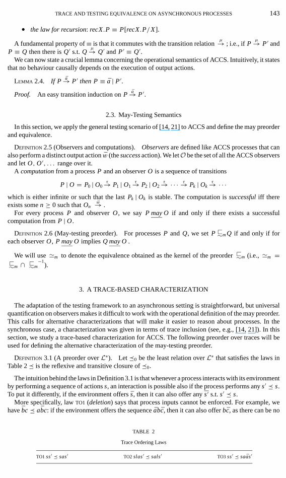
DEFINITION 3.1 (A preorder over L∗). Let �0 be the least relation over L∗ that satisfies the laws inTable 2 � is the reflexive and transitive closure of �0.
The intuition behind the laws in Definition 3.1 is that whenever a process interacts with its environmentby performing a sequence of actions s, an interaction is possible also if the process performs any s ′ � s.To put it differently, if the environment offers s, then it can also offer any s ′ s.t. s ′ � s.
More specifically, law TO1 (deletion) says that process inputs cannot be enforced. For example, wehave bc � abc: if the environment offers the sequence abc, then it can also offer bc, as there can be no
TABLE 2
Trace Ordering Laws
TO1 ss′ � sas′ TO2 slas′ � sals′ TO3 ss′ � saas′
144 BOREALE, DE NICOLA, AND PUGLIESE
causal dependence of bc upon the output a. Law TO2 (postponement) says that observations of processinputs can be delayed. For example, we have that bac � abc. Indeed, if the environment offers abcthen it can also offer bac. Finally, law TO3 (annihilation) allows the environment to internally consumepairs of complementary actions, e.g., b � aab. Indeed, if the environment offers aab, then a and a canbe internally consumed and b can be offered.
The preorder � is preserved by prefixing, since �0 is. Thus s ′ � s implies l · s ′ � l · s and s ′ · l � s · l.Building on the preorder � over traces, we can define a new preorder over processes.
DEFINITION 3.2 (Alternative preorder). For processes P and Q, we set P �m Q if and only ifwhenever P s⇒ then there exists s ′ such that s ′ � s and Q s ′⇒.
The difference with respect to the synchronous case (see, e.g., [14, 21]) is that we require a condi-tion weaker than trace inclusion by taking advantage of a preorder over single traces. We now provecoincidence of �m and ❁∼m. To do this, we need two preliminary results. First, we need to establish acrucial lemma that relates the preorder � to the operational semantics of ACCS.
LEMMA 3.3. Suppose that s ′ � s and that P s⇒. Then P s ′⇒.
Proof. It must be s ′(�0)ns, for some n ≥ 0.2 The proof proceeds by induction on n. The case n = 0is trivial. Suppose n > 0 and s ′(�0)n−1s ′′ �0 s. The thesis will follow by the induction hypothesis ifwe show that P s ′′⇒. To prove the latter we distinguish the possible cases for s ′′ �0 s, according tothe laws in Table 2, but analyze in detail only the cases of laws TO2 and TO3, case TO1 being similar toTO2.
• Law TO2. It must be s ′′ = rlar′ and s = ralr′. Since P s⇒, by virtue of Lemma 2.4 there areP ′, P ′′ s.t. P r⇒ P ′ a→ P ′′ lr ′==⇒ and P ′ ≡ a | P ′′. But then it holds also that P ′ lar ′−−→, hence the thesis.
• Law TO3. It must be s ′′ = rr ′ and s = raar ′. Since P s⇒, by virtue of Lemma 2.4 there areP ′, P ′′ s.t. P r⇒ P ′ a→ P ′′ ar ′==⇒ and P ′ ≡ a | P ′′. Since P ′′ a⇒, a communication between a and P ′′can take place, and as a result we get P ′ r ′⇒, hence the thesis.
We define below a special class of observers.
DEFINITION 3.4. Let s ∈ L∗. The observers o(s) are defined inductively as follows:
o(ε)def= w, o(as ′) def= a.o(s ′) and o(as ′) def= a | o(s ′).
LEMMA 3.5. Let s be a trace. If o(s) rw==⇒ then r � s.
Proof. We proceed by induction on s. We analyze only the case when s = as0, hence o(s) = a | o(s0);the other case is similar. There are three possibilities for r , depending on how the execution of actionsin o(s0) and of action a are interleaved.
1. o(s0) rw==⇒ (action a does not fire at all);
2. r = r1ar2 and o(s0)r1r2w====⇒ (action a fires);
3. r = r1r2 and o(s0)r1ar2w====⇒ (a and o(s0) interact with each other).
For case 1, the thesis follows from the induction hypothesis and law TO1. We analyze now case 2. Bythe induction hypothesis, r1r2 � s0; hence by prefixing ar1r2 � as0 = s. By repeated application oflaw TO2, we can move right a past r1 and get a smaller trace; i.e., r = r1ar2 � ar1r2 � s. Case 3 ishandled similarly, but relies on law TO3 instead of TO2.
We can now prove the following full abstraction theorem.
THEOREM 3.6 (Coincidence of ❁∼m and �m ). For all processes P and Q, P ❁∼m Q if and only ifP �m Q.
2 (�0)n stands for the identity relation if n = 0 and for the relation composition (�0)(n−1)· �0 otherwise.
TRACE AND TESTING EQUIVALENCE ON ASYNCHRONOUS PROCESSES 145
Proof. ‘Only if’ part. Suppose that P ❁∼m Q and that P s⇒: we must show that there exists s ′ � ssuch that Q s ′⇒. From P s⇒ and o(s) sw==⇒, we get P | o(s) w⇒; that is P may o(s). Hence Q may o(s);that is, Q | o(s) w⇒. This sequence of action can be unzipped as Q s ′⇒ and o(s) s ′w==⇒, for some trace s ′.From o(s) s ′w==⇒ and Lemma 3.5 we get s ′ � s, the wanted claim.
‘If’ part. Suppose that P �m Q and that P may O for any observer O: we must show that Q may Oas well. Now, P may O means that P | O w⇒. This sequence of transitions may be unzipped into twosequences P s⇒ and O sw==⇒, for some trace s. The hypothesis P �m Q implies that there exists s ′ � ssuch that Q s ′⇒. Now, s ′ � s implies s ′w � sw. Since O sw==⇒, by Lemma 3.3 we get that O s ′w==⇒.Combining this sequence with Q s ′⇒, we get that Q | O w⇒, i.e., the wanted Q may O .
The coincidence of ❁∼m and �m gives us a minimal set of observers for ❁∼m. Let M be the set ofobservers given in Definition 3.4, and let ❁∼
Mm
be the preorder over processes defined as in Definition 2.6,but considering only observers in M. The proof of the following corollary is an easy consequence ofLemma 3.5.
COROLLARY 3.7. For all processes P and Q, P ❁∼m Q if and only if P ❁∼Mm
Q.
The preorder ❁∼m can easily be proven to be a precongruence relying on the alternative characteri-zation �m . We omit the details.
EXAMPLE 3.8. We show some examples of pairs of processes related by the preorder. All of therelationships can be easily proven by using the alternative characterization of the preorder, �m .
• L(P) ⊆ L(Q) implies P ❁∼m Q; hence all the inequalities of the synchronous may preorderhold for ACCS.
• Since ε ∈ L(P) for each process P , from TO1 and TO3 in Table 2, we get a �m 0 and a.a �m 0.In particular, from a �m 0 we get a �m b and a.b �m b.a which imply that all processes containingonly input actions are equivalent to 0.
• An important law is a.(a | P) ❁∼m P . The converse does not hold; for instance, it is not true thatb ❁∼ma.(a | b) (just take the observer b.w).
• Another interesting law is a.(a | b) �m b. More generally, we have a.(a | G)+G �m G, whereG is a guarded summation
∑i∈I gi .Pi (a.a �m 0 is another instantiation of this general law).
4. A SET-THEORETIC INTERPRETATION
In this section we tackle the problem of defining a fully abstract interpretation of ACCS processes,i.e., a semantic mapping that assigns the same object to two processes only if they are may-equivalent.Furthermore, we demand that the interpretation be “finitary”: finite processes must be mapped to finitesets. We shall not deal here with the problem of defining a truly denotational semantics, which wouldalso assign a meaning to each operator of the calculus.
As an immediate consequence of Theorem 3.6, a fully abstract set-theoretic interpretation for ❁∼m
can be obtained by interpreting each P as the set of traces [[P]]m = {s | there is s ′ ∈ L(P)s.t. s ′ � s}and then ordering interpretations by set inclusion. However, this naive interpretation of processes is notsatisfactory, because it includes infinitely many traces even for finite processes; for instance, [[0]]m ={ε, a, aa, aaa, . . . , b, bb, . . . }. On the other hand, to simply set [[P]]m = L(P) would not yield a fullyabstract interpretation, as e.g., [[0]]m = {ε} �= {ε, a, aa} = [[a.a]]m .
In order to obtain a finitary fully abstract interpretation, we shall “minimize” the language of a processP , L(P), w.r.t. the trace preorder �. In the following, we use [s] to denote the �-equivalence class ofs, i.e., the set {s ′ | s ′ � s and s � s ′}. We first define the partial ordering of denotations.
DEFINITION 4.1.
• Consider a set D of �-equivalence classes. We say that D is a denotation if whenever [s], [s ′] ∈D and s � s ′ then [s] = [s ′]. We call D the set of all denotations.
• D is ordered by setting D1 ≤ D2 iff for each [s] ∈ D1 there is [s ′] ∈ D2 such that s ′ � s.
146 BOREALE, DE NICOLA, AND PUGLIESE
In words, a denotation D is a set of �-equivalence classes whose representative traces are not relatedby the preorder �. The next lemma follows by standard arguments: in particular, the antisymmetryproperty follows by minimality.
LEMMA 4.2. (D, ≤) is a partial ordering.
DEFINITION 4.3. For each P , we interpret P as the denotation
[[P]]mdef= {[s] | s ∈ L(P) and for each s ′ ∈ L(P) : s ′ � s implies [s] = [s ′] } .
EXAMPLE 4.4.
1. If Pdef= a.(a | b), we have that L(P) = {ε, a, aa, ab, aab, aba} and that ε is minimal in L(P)
(by TO1–TO3); hence [[a.(a | b)]]m = [[0]]m = { [ε] }.2. If Q
def= a | b.c, then L(Q) = {ε, a, ab, abc, b, ba, bac, bc, bca }. The set of �-minimal tracesof L(Q) is { ε, a, bc, abc, bca} and [[Q]]m = {[ε], [a], [bc], [abc], [bca]}.
3. If Qdef= a | b.c and R
def= a.P , then [[Q]]m = {[ε], [a], [bc], [abc], [bca]} and [[R]]m = { [ε],[abc], [aabc], [abca] }; hence [[R]]m ≤ [[Q]]m .
To prove the full-abstraction result (Theorem 4.6) we need a technical lemma.
LEMMA 4.5. Let C be a nonempty set of �-equivalence classes. Then C has minimal elements w.r.t.to the partial ordering defined by [s ′] ≤ [s] iff s ′ � s.
Proof. It is sufficient to show that there is no infinite descending chain · · · � s2 � s1 � s0, withdistinct si ’s. Note that whenever s ′ � s then |s ′| ≤ |s|, where | · | denotes size, and that actions appearingin s ′ are a subset of those appearing in s (formally, this fact is proven by induction on the number n s.t.s ′(�0)ns). Thus for any s, there are finitely many s ′ s.t. s ′ � s: this proves the lemma.
THEOREM 4.6. P ❁∼m Q if and only if [[P]]m ≤ [[Q]]m in D.
Proof. We use the alternative characterization �m of ❁∼m. Suppose that P �m Q; we show that[[P]]m ≤ [[Q]]m in D. Let [s] ∈ [[P]]m , with P s⇒. Then there is s ′ s.t. Q s ′⇒ and s ′ � s. Choose now [s0]which is minimal for the set {[s ′′] | s ′′ ∈ L(Q) and s ′′ � s ′ } and which exists by virtue of Lemma 4.5.By definition of [[·]]m , [s0] ∈ [[Q]]m , and moreover s0 � s.
Conversely, suppose that [[P]]m ≤ [[Q]]m in D: we show that P �m Q. Indeed, assume that P s⇒,for some s. Again, choose [s0] which is a minimal element for the set {[r ] | r ∈ L(P) and r � s } andwhich exists by virtue of Lemma 4.5. By definition of [[P]]m , [s0] ∈ [[P]]m , and moreover s0 � s. Thenthere is [s ′] ∈ [[Q]]m s.t. s ′ � s0 � s. Furthermore, by definition, Q s ′⇒, hence the thesis.
It is possible to give a concrete representation of equivalence classes.
PROPOSITION 4.7. Let s1 = m1 M1 · · · mn Mn, n ≥ 0, be any trace, where, for 1 ≤ i ≤ n, mi (resp.Mi ) is a trace containing only inputs (resp. outputs). Suppose that s2 � s1 and that s1 � s2. Then s2 isof the form m ′
1 M1 · · · m ′n Mn, where, for 1 ≤ i ≤ n, m ′
i is a permutation of mi .
Proof. For any trace r let d(r ) denote the number
( ∑a occurring in r
number of input actions that preceed a in r
)+ |r |.
As an example, d(cabcae) = (0 + 2 + 3) + 6 = 11. Each of the laws TO1, TO2, and TO3 makes d(·)decrease from right to left, except the instances of TO2 where l is an input action, which leave d(·)unchanged. Thus, if s1 � s2 and s2 � s1, it must be that d(s1) = d(s2). Hence, only instances of the lawTO2 where l is an input action can be used to deduce s1 � s2 (and s2 � s1): since these instances of thelaw only permit permutation of consecutive inputs, the thesis follows.
According to the above proposition, equivalence classes of traces can be viewed as sequences wheremultisets of input actions alternate with sequences of output actions (that is, as elements of ( mul(N ) ∪
TRACE AND TESTING EQUIVALENCE ON ASYNCHRONOUS PROCESSES 147
N ∗)∗, where mul(N ) is the set of finite multisets of N ). This model can be further optimized. For
example, when defining [[·]]m it is possible to enrich the theory of � with a commutativity law foroutputs (ab � ba): this would permit one to regard sequences of outputs as multisets and would yieldmore compact denotations of processes. For instance, the denotation of process Q in Example 4.4would reduce to {[ε], [a], [bc], [abc]}. A similar optimization will be used in the definition of canonicalprocesses in the next section.
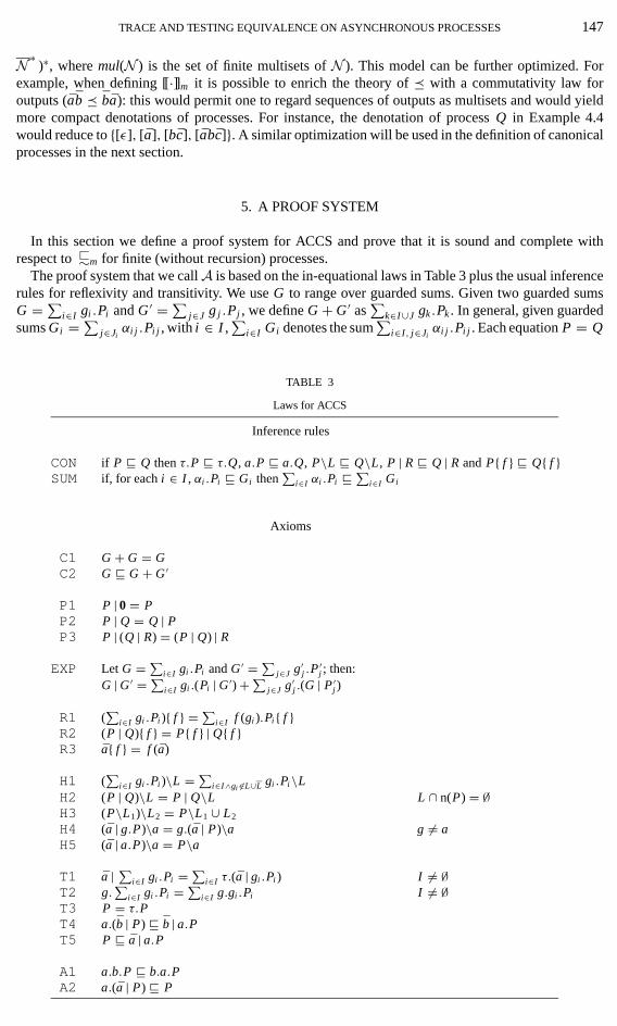
5. A PROOF SYSTEM
In this section we define a proof system for ACCS and prove that it is sound and complete withrespect to ❁∼m for finite (without recursion) processes.
The proof system that we call A is based on the in-equational laws in Table 3 plus the usual inferencerules for reflexivity and transitivity. We use G to range over guarded sums. Given two guarded sumsG = ∑
i∈I gi .Pi and G ′ = ∑j∈J g j .Pj , we define G + G ′ as
∑k∈I∪J gk .Pk . In general, given guarded
sums Gi = ∑j∈Ji
αi j .Pi j , with i ∈ I ,∑
i∈I Gi denotes the sum∑
i∈I, j∈Jiαi j .Pi j . Each equation P = Q
TABLE 3
Laws for ACCS
Inference rules
CON if P � Q then τ.P � τ.Q, a.P � a.Q, P\L � Q\L , P | R � Q | R and P{ f } � Q{ f }SUM if, for each i ∈ I , αi .Pi � Gi then
∑i∈I αi .Pi � ∑
i∈I Gi
Axioms
C1 G + G = GC2 G � G + G ′
P1 P | 0 = PP2 P | Q = Q | PP3 P | (Q | R) = (P | Q) | R
EXP Let G = ∑i∈I gi .Pi and G ′ = ∑
j∈J g′j .P
′j ; then:
G | G ′ = ∑i∈I gi .(Pi | G ′) + ∑
j∈J g′j .(G | P ′
j )
R1 (∑
i∈I gi .Pi ){ f } = ∑i∈I f (gi ).Pi { f }
R2 (P | Q){ f } = P{ f } | Q{ f }R3 a{ f } = f (a)
H1 (∑
i∈I gi .Pi )\L = ∑i∈I∧gi �∈L∪L gi .Pi\L
H2 (P | Q)\L = P | Q\L L ∩ n(P) = ∅H3 (P\L1)\L2 = P\L1 ∪ L2
H4 (a | g.P)\a = g.(a | P)\a g �= aH5 (a | a.P)\a = P\a
T1 a | ∑i∈I gi .Pi = ∑
i∈I τ.(a | gi .Pi ) I �= ∅T2 g.
∑i∈I gi .Pi = ∑
i∈I g.gi .Pi I �= ∅T3 P = τ.PT4 a.(b | P) � b | a.PT5 P � a | a.P
A1 a.b.P � b.a.PA2 a.(a | P) � P

148 BOREALE, DE NICOLA, AND PUGLIESE
is an abbreviation for the pair of inequations P � Q and Q � P . We write P �A Q (P =A Q) toindicate that P � Q (P = Q) can be derived within the proof system A.
Laws A1 and A2 differentiate asynchronous from synchronous may-testing: they are not sound forthe synchronous may preorder [14]. In particular, law A1 states that processes are insensitive to thearrival ordering of messages from the environment, while law A2 states that any execution of P thatdepends on the availability of a message a is worse than P itself, even if a is immediately re-issued.The other laws in Table 3 are sound also for the synchronous may-testing [14]. The laws in Table 3 canbe easily proven sound by taking advantage of the preorder �m . Let us now consider two importantderived laws:
• (D1) a.P �A P and
• (D2) 0 �A a.
Law D2 easily follows from T3 and C2, as, for any P , 0 �A τ.P =A P . The inequality D1 can beinferred by first noting that from D2 it follows that P �A a | P , which implies a.P �A a.(a | P), thenapplying A2. In particular, we have that a �A 0. From 0 �A P , for any P , and a.a =A a.(a | 0) �A 0(law A2), we also get a.a =A 0.
For proving completeness of the proof system, we shall rely on the existence of canonical formsfor processes, which are unique up to commutativity of parallel composition and up to permutation ofconsecutive input actions. The canonical form of a process will be obtained by first minimizing its setof traces and then summing up the resulting traces into a guarded sum. To guarantee uniqueness, itis convenient to extend � via a commutativity law for output actions: this prevents us from having toconsider all traces that arise from different permutations of parallel output actions (like in a | b, notethat traces ab and ba are not related by �).
DEFINITION 5.1 (The preorder �|). We let �| be the reflexive and transitive closure of the binaryrelation over traces induced by the laws TO1–TO3 plus law:
(T O4) sabs ′ � sbas ′.
Of course, � is included in �|.
DEFINITION 5.2 (Canonical forms).
• Given s ∈ L∗, the process t(s) is defined by induction on s as follows: t(ε)def= 0, t(as ′) def= a.t(s ′),
and t(as ′) def= a | t(s ′).• Consider A ⊆fin L∗. We say that A is:
—complete if whenever t(r ) s⇒, for r ∈ A, then there is s ′ ∈ A s.t. s ′ �| s;
—minimal if whenever s, s ′ ∈ A and s ′ �| s then s ′ = s.
• A canonical form is a process of the form∑
s∈A−{ε} τ.t(s), for some A ⊆fin L∗ which is bothcomplete and minimal.
Note that a complete set of traces always contains the empty trace ε. The proof of uniqueness ofcanonical forms can be decomposed into three simple lemmas.
LEMMA 5.3. If t(s) s ′⇒ then t(s ′) �A t(s).
Proof. The proof proceeds by induction on the length of s. The most interesting case is whens = as0, for some s0; hence t(s) = a | t(s0). Then there are three cases for s ′:
1. t(s0) s ′⇒;
2. s ′ = r ar ′ and t(s0) rr ′==⇒, for some traces r and r ′;3. s ′ = rr ′ and t(s0) rar ′===⇒, for some traces r and r ′.
For case 1 the thesis follows from P �A a | P (by D2) and the induction hypothesis. For case 2, fromthe induction hypothesis we get that t(rr ′) �A t(s0); hence a | t(rr ′) �A a | t(s0) = t(s); from repeated
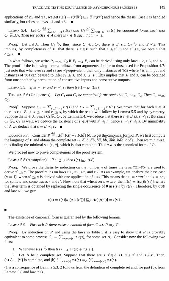
TRACE AND TESTING EQUIVALENCE ON ASYNCHRONOUS PROCESSES 149
applications of P2 and T4, we get t(s ′) = t(r ar ′) �A a | t(rr ′) and hence the thesis. Case 3 is handledsimilarly, but relies on laws T4 and T5.
LEMMA 5.4. Let C1def= ∑
s∈A−{ε} τ.t(s) and C2def= ∑
r∈B−{ε} τ.t(r ) be canonical forms such thatC1
❁∼mC2. Then for each s ∈ A there is r ∈ B such that r �| s.
Proof. Let s ∈ A. Then C1s⇒, thus, since C1 �m C2, there is s ′ s.t. C2
s ′⇒ and s ′ � s. Thisimplies, by completeness of B, that there is r ∈ B such that r �| s ′. Since s ′ � s, we obtain thatr �| s.
In what follows, we write P1 =AC P2 if P1 =A P2 can be derived using only laws P2, P3, and A1.The proof of the following lemma follows from arguments similar to those used for Proposition 4.7:just note that whenever s1 and s2 are �|-equivalent, then only instances of TO2 where l is an input andinstances of TO4 can be used to infer s1 �| s2 and s2 �| s1. This implies that s1 and s2 can be obtainedfrom one another by permutation of consecutive inputs and consecutive outputs.
LEMMA 5.5. If s1 �| s2 and s2 �| s1 then t(s1) =AC t(s2).
THEOREM 5.6 (Uniqueness). Let C1 and C2 be canonical forms such that C1 �m C2. Then C1 =AC
C2.
Proof. Suppose C1 = ∑s∈A−{ε} τ.t(s) and C2 = ∑
r∈B−{ε} τ.t(r ). We prove that for each s ∈ Athere is r ∈ B s.t. s �| r and r �| s, by which the result will follow by Lemma 5.5 and by symmetry.Suppose that s ∈ A. Since C1
❁∼mC2, by Lemma 5.4, we deduce that there is r ∈ B s.t. r �| s. But sinceC2
❁∼m C1 as well, we deduce the existence of s ′ ∈ A with s ′ �| r ; hence s ′ �| r �| s. By minimalityof A we deduce that s = s ′ �| r .
EXAMPLE 5.7. Consider Pdef= τ.(a | b.b)+τ.b.(a | b). To get the canonical form of P , we first compute
the language of P and obtain the complete set {ε, a, b, ab, ba, bb, abb, bab, bba}. Then we minimize,thus finding the minimal set {ε, a}, which is also complete. Thus τ.a is the canonical form of P .
We proceed now to prove completeness of the proof system.
LEMMA 5.8 (Absorption). If s ′ �| s then t(s) �A t(s ′).
Proof. We prove the thesis by induction on the number n of times the laws TO1–TO4 are used toderive s ′ �| s. The proof relies on laws D1, D2, A2, and P2. As an example, we analyze the base case(n = 1), when s ′ �| s is derived with one application of TO3. This means that s ′ = raar ′ and s = rr ′,for some a and some traces r and r ′. Now, note that whenever s = s1s2 then t(s) = t(s1)[t(s2)], wherethe latter term is obtained by replacing the single occurrence of 0 in t(s1) by t(s2). Therefore, by CONand law A2, we get:
t(s) = t(r )[a.(a | t(r ′))] �A t(r )[t(r ′)] = t(s ′) .
The existence of canonical form is guaranteed by the following lemma.
LEMMA 5.9. For each P there exists a canonical form C s.t. P =A C.
Proof. By induction on P and using the laws in Table 3 it is easy to show that P is provablyequivalent to some process C1 = ∑
s∈A1−{ε} τ.t(s), for some set A1. Consider now the following twofacts:
1. Whenever t(s) s ′⇒ then t(s) =A τ.t(s) + τ.t(s ′).2. Let A be a complete set. Suppose that there are s, s ′ ∈ A s.t. s �| s ′ and s �= s ′. Then,
(a) A − {s ′} is complete, and (b)∑
r∈A−{ε} τ.t(r ) =A∑
r∈A−{ε,s ′} τ.t(r ).
(1 is a consequence of Lemma 5.3; 2 follows from the definition of complete set and, for part (b), fromLemma 5.8 and law C1).
150 BOREALE, DE NICOLA, AND PUGLIESE
By repeatedly applying 1, we can saturate A1, thus proving C1 equivalent to a summation C2 over acomplete set A2. Then, by repeatedly applying 2, we can remove redundant traces in A2, thus provingC2 equivalent to a summation over a complete and minimal set of traces.
THEOREM 5.10 (Completeness). For finite processes P and Q, P ❁∼m Q implies P �A Q.
Proof. Lemma 5.9 allows us to assume that both P and Q are in canonical form: Pdef= ∑
s∈A−{ε} τ.t(s)and Q
def= ∑r∈B−{ε} τ.t(r ). It is sufficient to show that for each s ∈ A there is r ∈ B s.t. t(s) �A t(r ),
by which the thesis will follows thanks to the law C2. But this fact follows by Lemmas 5.4 and 5.8.
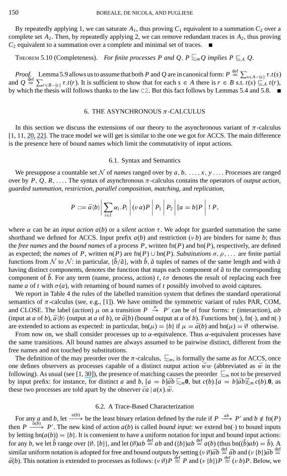
6. THE ASYNCHRONOUS π -CALCULUS
In this section we discuss the extensions of our theory to the asynchronous variant of π -calculus[1, 11, 20, 22]. The trace model we will get is similar to the one we got for ACCS. The main differenceis the presence here of bound names which limit the commutativity of input actions.
6.1. Syntax and Semantics
We presuppose a countable set N of names ranged over by a, b, . . . , x, y . . . . Processes are rangedover by P, Q, R, . . . . The syntax of asynchronous π -calculus contains the operators of output action,guarded summation, restriction, parallel composition, matching, and replication,
P ::= a〈b〉∣∣∣∣ ∑
i∈I
αi .Pi
∣∣∣∣ (ν a)P
∣∣∣∣ P1
∣∣∣∣ P2
∣∣∣∣ [a = b]P
∣∣∣∣ ! P,
where α can be an input action a(b) or a silent action τ . We adopt for guarded summation the sameshorthand we defined for ACCS. Input prefix a(b) and restriction (ν b) are binders for name b; thusthe free names and the bound names of a process P , written fn(P) and bn(P), respectively, are definedas expected; the names of P , written n(P) are fn(P) ∪ bn(P). Substitutions σ, ρ, . . . are finite partialfunctions from N to N : in particular, {b/a}, with b, a tuples of names of the same length and with ahaving distinct components, denotes the function that maps each component of a to the correspondingcomponent of b. For any term (name, process, action) t , tσ denotes the result of replacing each freename a of t with σ (a), with renaming of bound names of t possibly involved to avoid captures.
We report in Table 4 the rules of the labelled transition system that defines the standard operationalsemantics of π -calculus (see, e.g., [1]). We have omitted the symmetric variant of rules PAR, COM,and CLOSE. The label (action) µ on a transition P
µ→ P ′ can be of four forms: τ (interaction), ab(input at a of b), a〈b〉 (output at a of b), or a(b) (bound output at a of b). Functions bn(·), fn(·), and n(·)are extended to actions as expected: in particular, bn(µ) = {b} if µ = a(b) and bn(µ) = ∅ otherwise.
From now on, we shall consider processes up to α-equivalence. Thus α-equivalent processes havethe same transitions. All bound names are always assumed to be pairwise distinct, different from thefree names and not touched by substitutions.
The definition of the may preorder over the π -calculus, ❁∼m, is formally the same as for ACCS, onceone defines observers as processes capable of a distinct output action ww (abbreviated as w in thefollowing). As usual (see [1, 30]), the presence of matching causes the preorder ❁∼m not to be preservedby input prefix: for instance, for distinct a and b, [a = b]ab ❁∼m0, but c(b).[a = b]ab /❁∼m c(b).0, asthese two processes are told apart by the observer ca | a(x).w.
6.2. A Trace-Based Characterization
For any a and b, leta(b)−−→ be the least binary relation defined by the rule if P ab−−→ P ′ and b /∈ fn(P)
then Pa(b)−−→ P ′. The new kind of action a(b) is called bound input: we extend bn(·) to bound inputs
by letting bn(a(b)) = {b}. It is convenient to have a uniform notation for input and bound input actions:for any b, we let b range over {∅, {b}}, and let (∅)ab
def= ab and ({b})abdef= a(b) (thus bn((b)ab) = b). A
similar uniform notation is adopted for free and bound outputs by setting (ν ∅)abdef= ab and (ν {b})ab
def=a(b). This notation is extended to processes as follows: (ν ∅)P
def= P and (ν {b})Pdef= (ν b)P . Below, we
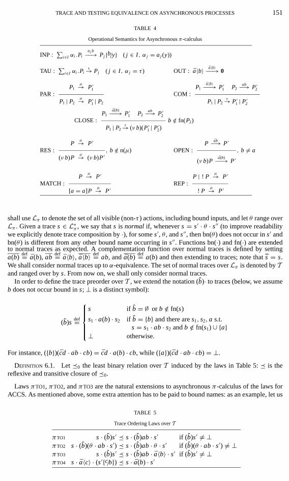
TRACE AND TESTING EQUIVALENCE ON ASYNCHRONOUS PROCESSES 151
TABLE 4
Operational Semantics for Asynchronous π -calculus
INP :∑
i∈I αi .Pia j b−−→ Pj {b/y} ( j ∈ I, α j = a j (y))
TAU :∑
i∈I αi .Piτ→ Pj ( j ∈ I, α j = τ ) OUT : a〈b〉 a〈b〉−−→ 0
PAR :P1
µ→ P ′1
P1 | P2µ→ P ′
1 | P2
COM :P1
a〈b〉−−→ P ′1 P2
ab−→ P ′2
P1 | P2τ→ P ′
1 | P ′2
CLOSE :P1
a(b)−−→ P ′1 P2
ab−→ P ′2
P1 | P2τ→ (ν b)(P ′
1 | P ′2)
b /∈ fn(P2)
RES :P
µ→ P ′
(ν b)Pµ→ (ν b)P ′
, b /∈ n(µ) OPEN :P ab−→ P ′
(ν b)Pa(b)−−→ P ′
, b �= a
MATCH :P
µ→ P ′
[a = a]Pµ→ P ′
REP :P | ! P
µ→ P ′
! Pµ→ P ′
shall use Lπ to denote the set of all visible (non-τ ) actions, including bound inputs, and let θ range overLπ . Given a trace s ∈ L∗
π , we say that s is normal if, whenever s = s ′ · θ · s ′′ (to improve readabilitywe explicitly denote trace composition by ·), for some s ′, θ , and s ′′, then bn(θ ) does not occur in s ′ andbn(θ ) is different from any other bound name occurring in s ′′. Functions bn(·) and fn(·) are extendedto normal traces as expected. A complementation function over normal traces is defined by settinga(b)
def= a(b), abdef= a〈b〉, a〈b〉 def= ab, and a(b)
def= a(b) and then extending to traces; note that s = s.We shall consider normal traces up to α-equivalence. The set of normal traces over Lπ is denoted by Tand ranged over by s. From now on, we shall only consider normal traces.
In order to define the trace preorder over T , we extend the notation (b)· to traces (below, we assumeb does not occur bound in s; ⊥ is a distinct symbol):
(b)sdef=
s if b = ∅ or b /∈ fn(s)
s1 · a(b) · s2 if b = {b} and there are s1, s2, a s.t.s = s1 · ab · s2 and b /∈ fn(s1) ∪ {a}
⊥ otherwise.
For instance, ({b})(cd · ab · cb) = cd · a(b) · cb, while ({a})(cd · ab · cb) = ⊥.
DEFINITION 6.1. Let �0 the least binary relation over T induced by the laws in Table 5: � is thereflexive and transitive closure of �0.
Laws πTO1, πTO2, and πTO3 are the natural extensions to asynchronous π -calculus of the laws forACCS. As mentioned above, some extra attention has to be paid to bound names: as an example, let us
TABLE 5
Trace Ordering Laws over T
πTO1 s · (b)s ′ � s · (b)ab · s ′ if (b)s ′ �= ⊥πTO2 s · (b)(θ · ab · s ′) � s · (b)ab · θ · s ′ if (b)(θ · ab · s ′) �= ⊥πTO3 s · (b)s ′ � s · (b)ab · a〈b〉 · s ′ if (b)s ′ �= ⊥πTO4 s · a〈c〉 · (s ′{c/b}) � s · a(b) · s ′
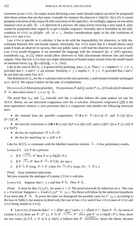
152 BOREALE, DE NICOLA, AND PUGLIESE
comment on law πTO2. An output action declaring a new name (bound output) can never be postponedafter those actions that use that name. Consider for instance the observer (ν b)(a〈b〉 | b(c).O): it cannotpostpone execution of the output ab after execution of the input b(c). Accordingly, suppose an executionsequence such as a(b) · bc · s is observed of a process: the input action receiving a new name b, a(b),cannot be postponed after output bc to get a smaller sequence. Formally, this is forbidden by the side-condition of πTO2, as ({b})(bc · ab · s) = ⊥. Similar considerations apply to the side conditions oflaws πTO1 and πTO3.
Law πTO4 is specific to π -calculus: it has to do with the impossibility, for observers, to fully dis-criminate between free and bound outputs. Informally, law πTO4 states that if a bound (hence new)name b leads an observer to success, then any public name c will lead the observer to success as well.Law πTO4 would disappear if we extended the language with the mismatch ([a �= b]P) operator,considered, e.g., in [7], which would allow observers to fully discriminate between free and boundoutputs. Note that law πTO4 does not imply elimination of bound output actions from the model basedon minimal traces; e.g., [[(ν a)(ca)]]m = {ε, c(a)}.
Like in the case of ACCS, � is preserved by prefixing, since �0 is. Thus s ′ � s implies θ · s ′ � θ · s,provided that θ · s and θ · s ′ are normal. Similarly, s ′ � s implies s ′ · θ � s · θ , provided that s and s ′
do not bind any name free in θ .The definition of �m for the π -calculus relies on the trace preorder � and remains formally unchanged
w.r.t. ACCS. We repeat it below for the sake of completeness.
DEFINITION 6.2 (Alternative preorder). For processes P and Q, we let P �m Q if and only if wheneverP s⇒ then there exists s ′ � s s.t. Q s ′⇒ .
The proof that �m and ❁∼m coincide over the π -calculus follows the same pattern we saw forACCS. Below, we use structural congruence over the π -calculus. Structural congruence [29] is theleast equivalence relation ≡ over processes that is a congruence and satisfies the following structurallaws:
• the monoid laws for parallel composition: P | 0 ≡ P , P | Q ≡ Q | P , and P | (Q | R) ≡(P | Q) | R;
• the laws for restriction: (ν b)0 ≡ 0, (ν a)(ν b)P ≡ (ν b)(ν a)P , and (ν a)(P | Q) ≡ P | (ν a)Q ifa �∈ fn(P);
• the law for replication: !P ≡ P | !P .
• the law for matching: [a = a]P ≡ P .
Like for ACCS, ≡ commutes with the labelled transition relationµ→ . A few preliminary results.
LEMMA 6.3. Let P be a process.
1. If P(ν b)ab−−−−→ P ′ then P ≡ (ν b)(ab | P ′).
2. If Pa(b)−−→ P ′ then P ac−→ P ′{c/b}, for any c.
3. If P θ→ P ′ (resp. P τ→ P ′ ) then Pσθσ−→ P ′σ (resp. Pσ
τ→ P ′σ ).
Proof. Easy transition inductions.We now examine the analogue of Lemma 3.3 for π -calculus.
LEMMA 6.4. Suppose that s ′ � s and that P s⇒ . Then P s ′⇒ .
Proof. It must be that s ′(�0)ns, for some n ≥ 0. The proof proceeds by induction on n. The casen = 0 is trivial. Suppose n > 0 and s ′(�0)n−1s ′′ �0 s. The thesis will follow by the induction hypothesisif we show that P s ′′⇒ . To prove the latter we distinguish the possible cases for s ′′ �0 s, according tothe laws in Table 5, but analyze in detail only the case of law πTO2 and of law πTO4 (cases of πTO1 andπTO3 being similar to πTO2).
• Law πTO2. It must be that s ′′ = r ·(b)(θ ·ab ·r ′) and s = r ·(b)ab ·θ ·r ′. Since P s⇒ , by virtue ofLemma 6.3 (1) there are P ′, P ′′ s.t. P r⇒ P ′ (ν b)ab−−−−→ P ′′ θ ·r ′==⇒ and P ′ ≡ (ν b)(ab | P ′′). Now, thereare two cases: (i) if b = ∅ or b /∈ fn(θ ), it follows that P ′ θ ·(ν b)ab·r ′=======⇒, hence the thesis, because
TRACE AND TESTING EQUIVALENCE ON ASYNCHRONOUS PROCESSES 153
(b)(θ · ab · r ′) = θ · (b)ab · r ′; (ii) if b = {b} and b ∈ fn(θ ), then it must be θ = cb for some c �= b
(otherwise it would be (b)(θ · ab · r ′) = ⊥), hence P ′ c(b)·ab·r ′======⇒, which implies the thesis for this case,because (b)(θ · ab · r ′) = c(b) · ab · r ′.
• Law πTO4. Suppose s ′′ = r · a〈c〉 · (r ′{c/b}) and s = r · a(b) · r ′. Now, P s⇒ means that there
are P ′, P ′′ s.t. P r⇒ P ′ a(b)−−→ P ′′ r ′⇒ . By Lemma 6.3(2) P ′ ac−→ P ′′{c/b}, and by repeated application
of Lemma 6.3(3) P ′′ r ′{c/b}====⇒, hence the thesis for this case.
DEFINITION 6.5 (Canonical observers). Let s be a trace. The observer o(s) is defined by induction ons as follows:
o(ε)def= w
o(a(b) · s ′) def= (ν b)(a〈b〉 | o(s ′)) o(a〈b〉 · s ′) def= a(x).[x = b]o(s ′) (x fresh)
o(ab · s ′) def= a〈b〉 | o(s ′) o(a(b) · s ′) def= a(b).o(s ′).
We now examine the analogue of Lemma 3.5 for π -calculus.
LEMMA 6.6. Let s be a trace. If o(s) r ·w==⇒ then r � s.
Proof. We proceed by induction on s. We analyze only the case when s = a(b) · s0, hence o(s) =(ν b)(a〈b〉 | o(s0)), which is the most difficult. There are three possible cases for r , depending on howthe execution of actions in o(s0) and of action a〈b〉 are interleaved: in case (1) a〈b〉 does not fire at all,in case (2) a〈b〉 fires, and in case (3) a〈b〉 and o(s0) interact with each other. Each of these three casesis in turn divided into two subcases, depending on whether and how restriction (ν b) is extruded (byvirtue of rule OPEN):
(1a) o(s0) r ·w==⇒;
(1b) r = r1 · a′(b) · r2 and o(s0)r1·a′b·r2·w======⇒;
(2a) r = r1 · a(b) · r2 and o(s0)r1·r2·w====⇒;
(2b) r = r1 · a′(b) · r2 · a〈b〉 · r3 and o(s0)r1·a′b·r2·r3·w========⇒;
(3a) r = r1 · r2 and o(s0)r1·a(b)·r2·w=======⇒;
(3b) r = r1 · a′(b) · r2 · r3 and o(s0)r1·a′(b)·r2·ab·r3·w==========⇒.
For cases (1a–1b), the thesis follows from the induction hypothesis and law πTO1. We analyze now case(2b), because (2a) is easier. By the induction hypothesis, r1 ·a′b ·r2 ·r3 � s0, hence a(b) ·r1 ·a′b ·r2 ·r3 �a(b) · s0 = s. By repeated applications of law πTO2 we can move right a(b) (note that b /∈ n(r1)) andget first that r1 · a(b) · a′b · r2 · r3 � s and then that r1 · a′(b) · ab · r2 · r3 � s. Finally, by moving rightab, we get that r = r1 · a′(b) · r2 · ab · r3 � s. Cases (3a–3b) are handled similarly, but relying on lawπTO3 (and, for (3b), on πTO4) instead of πTO2.
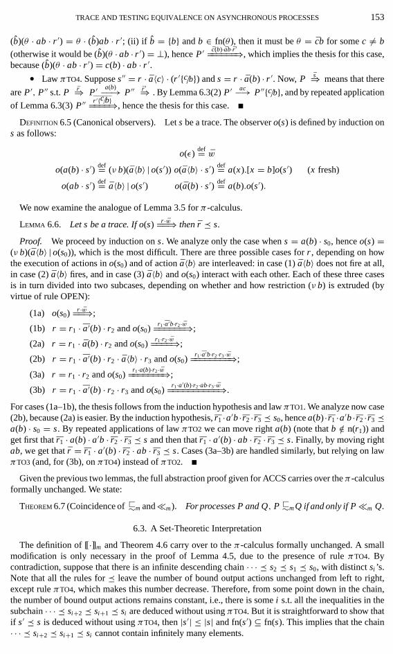
Given the previous two lemmas, the full abstraction proof given for ACCS carries over the π -calculusformally unchanged. We state:
THEOREM 6.7 (Coincidence of ❁∼m and �m). For processes P and Q, P ❁∼m Q if and only if P �m Q.
6.3. A Set-Theoretic Interpretation
The definition of [[·]]m and Theorem 4.6 carry over to the π -calculus formally unchanged. A smallmodification is only necessary in the proof of Lemma 4.5, due to the presence of rule πTO4. Bycontradiction, suppose that there is an infinite descending chain · · · � s2 � s1 � s0, with distinct si ’s.Note that all the rules for � leave the number of bound output actions unchanged from left to right,except rule πTO4, which makes this number decrease. Therefore, from some point down in the chain,the number of bound output actions remains constant, i.e., there is some i s.t. all the inequalities in thesubchain · · · � si+2 � si+1 � si are deduced without using πTO4. But it is straightforward to show thatif s ′ � s is deduced without using πTO4, then |s ′| ≤ |s| and fn(s ′) ⊆ fn(s). This implies that the chain· · · � si+2 � si+1 � si cannot contain infinitely many elements.
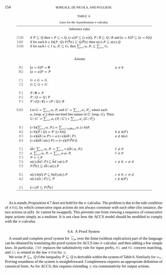
154 BOREALE, DE NICOLA, AND PUGLIESE
TABLE 6
Laws for the Asynchronous π -calculus
Inference rules
CON if P � Q then τ.P � τ.Q, (ν a)P � (ν a)Q, P | R � Q | R and [a = b]P � [a = b]QINP if for each b ∈ fn(P, Q) P{b/x} � Q{b/x} then a(x).P � a(x).QSUM if for each i ∈ I αi .Pi � Gi then
∑i∈I αi .Pi � ∑
i∈I Gi
Axioms
M1 [a = b]P = 0 a �= bM2 [a = a]P = P
C1 G + G = GC2 G � G + G ′
P1 P | 0 = PP2 P | Q = Q | PP3 P | (Q | R) = (P | Q) | R
EXP Let G = ∑i∈I αi .Pi and G ′ = ∑
j∈J α′j .P
′j , where each
αi (resp. α′j ) does not bind free names of G ′ (resp. G). Then:
G | G ′ = ∑i∈I αi .(Pi | G ′) + ∑
j∈J α′j .(G | P ′
j )
H1 (ν b)(∑
i∈I αi .Pi ) = ∑i∈I∧b/∈n(αi ) αi .(ν b)Pi
H2 (ν b)(P | Q) = P | (ν b)Q b /∈ n(P)H3 (ν a)(ab | α.P) = α.(ν a)(ab | P) a /∈ n(α)H4 (ν a)(ab | a(c).P) = (ν a)(P{b/c})
T1 ab | ∑i∈I αi .Pi = ∑
i∈I τ.(ab | αi .Pi ) I �= ∅T2 α.
∑i∈I αi .Pi = ∑
i∈I α.αi .Pi I �= ∅T3 P = τ.PT4 a(c).(bd | P) � bd | a(c).P c �= b, c �= dT5 P{b/c} � ab | a(c).P
A1 a(c).b(d).P � b(d).a(c).P c �= b, c �= dA2 a(c).(ac | P) � P c /∈ n(P)
S1 (ν c)P � P{b/c}
As is stands, Proposition 4.7 does not hold for the π -calculus. The problem is due to the side conditionof πTO2, by which consecutive input actions do not always commute with each other (for instance, thetwo actions in a(b) · bc cannot be swapped). This prevents one from viewing a sequence of consecutiveinput actions simply as a multiset. It is not clear how the ACCS model should be modified to complywith the π -calculus.
6.4. A Proof System
A sound and complete proof system for ❁∼m over the finite (without replication) part of the languagecan be obtained by translating the proof system for ACCS into π -calculus and then adding a few simplelaws. In particular, INP replaces the substitutivity rule for input prefix, M1 and M2 concern matching,and S1 is related to the law πTO4 for �.
We write P �π Q if the inequality P � Q is derivable within the system of Table 6. Similarly for =π .Proving soundness of the system is straightforward. Completeness requires an appropriate definition ofcanonical form. As for ACCS, this requires extending � via commutativity for output actions.
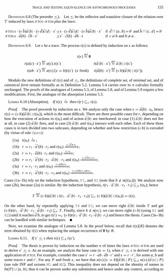
TRACE AND TESTING EQUIVALENCE ON ASYNCHRONOUS PROCESSES 155
DEFINITION 6.8 (The preorder �|). Let �| be the reflexive and transitive closure of the relation overT induced by laws πTO1–πTO4 plus the laws:
πTO5 s · (ν b)a〈b〉 · (ν d)c〈d〉 · s ′ �s · (ν d)c〈d〉 · (ν b)a〈b〉 · s ′ if d ∩ {a, b} = ∅ and b ∩ {c, d} = ∅πTO6 s · a(b) · cb · s ′ �s ′ · c(b) · ab · s if c �= b and b �= a.
DEFINITION 6.9. Let s be a trace. The process t(s) is defined by induction on s as follows:
t(ε)def= 0
t(a(c) · s ′) def= a(c).t(s ′) t(a〈b〉 · s ′) def= a〈b〉 | t(s ′)
t(ab · s ′) def= a(x).[x = b]t(s ′) (x fresh) t(a(b) · s ′) def= (ν b)(a〈b〉 | t(s ′)).
Modulo the new definitions of t(s) and of �|, the definitions of complete set, of minimal set, and ofcanonical form remain formally as in Definition 5.2. Lemma 5.4 carries over to π -calculus formallyunchanged. The proofs of the analogues of Lemma 5.3, of Lemma 5.8, and of Lemma 5.9 require a fewmodifications. First, the analogue of the absorption Lemma 5.3.
LEMMA 6.10 (Absorption). If t(s) r⇒ then t(r ) �π t(s).
Proof. The proof proceeds by induction on s. We analyze only the case when s = a(b) · s0, hencet(s) = (ν b)(a〈b〉 | t(s0)), which is the most difficult. There are three possible cases for r , depending onhow the execution of actions in t(s0) and of action a〈b〉 are interleaved: in case (1) a〈b〉 does not fireat all, in case (2) a〈b〉 fires, and in case (3) a〈b〉 and t(s0) interact with each other. Each of these threecases is in turn divided into two subcases, depending on whether and how restriction (ν b) is extruded(by virtue of rule Open):
(1a) t(s0) r⇒ ;
(1b) r = r1 · a′(b) · r2 and t(s0)r1·a′b·r2=====⇒;
(2a) r = r1 · a(b) · r2 and t(s0)r1·r2===⇒;
(2b) r = r1 · a′(b) · r2 · a〈b〉 · r3 and t(s0)r1·a′b·r2·r3======⇒;
(3a) r = r1 · r2 and t(s0)r1·a(b)·r2=====⇒;
(3b) r = r1 · a′(b) · r2 · r3 and t(s0)r1·a′(b)·r2·ab·r3=========⇒.
Cases (1a–1b) rely on the induction hypothesis, P1, and H2 (note that b /∈ n(t(s0))). We analyze nowcase (2b), because (2a) is similar. By the induction hypothesis, t(r1 · a′〈b〉 · r2 · r3) �A t(s0); hence
Tdef= (ν b)(a〈b〉 | t(r1 · a′〈b〉 · r2 · r3)) �π (ν b)(a〈b〉 | t(s0)) = t(s).
On the other hand, by repeatedly applying T4 and P2, we can move right a〈b〉 inside T and get(ν b)t(r1 · a′〈b〉 · r2 · a〈b〉 · r3) �π T . Finally, since b /∈ n(σ1), we can move right (ν b) (using H1 andH2) until it reaches a′b, to get t(r ) =π (ν b)t(r1 · a′〈b〉 ·r2 · a〈b〉 ·r3) and hence the thesis. Cases (3a–3b)can be handled with similar techniques.
Next, we examine the analogue of Lemma 5.8. In the proof below, recall that t(s)[R] denotes theterm obtained by t(s) when replacing the unique occurrence of 0 by R.
LEMMA 6.11. If s ′ �| s then t(s) �A t(s ′).
Proof. The thesis is proven by induction on the number n of times the laws πTO1–πTO6 are usedto derive s ′ �| s. As an example, we analyze the base case (n = 1), when s ′ �| s is derived with oneapplication of πTO3. For example, consider the case s ′ = r · ab · ab · r ′ and s = r · r ′, for some a, b andsome traces r and r ′. For any P and fresh x , we have that a(x).[x = b](a〈b〉 | P) �A a(x).(a〈x〉 | P)(use rule INP and axioms M1 and M2). This inequality does not depend on the identity of names infn(P) ∪ {a, b}; thus it can be proven under any substitution and hence under any context, according to
156 BOREALE, DE NICOLA, AND PUGLIESE
the congruence rules of the proof system. From this fact and A2, we get:
t(s) = t(r )[a(x).[x = b](ab | t(r ′))] �A t(r )[a(x).(ax | t(r ′))] �A t(r )[t(r ′)] = t(s ′) .
We turn to the existence of provably equivalent canonical forms, the analogue of Lemma 5.9. Withrespect to ACCS, the proof presents an additional difficulty, due to the peculiar form of the input prefixsubstitutivity rule (INP) in π -calculus. When proving P equivalent to a sum of t(s)’s, this rule will notlet plain structural induction on P work.
LEMMA 6.12. For each P there exists a canonical form C s.t. P =π C.
Proof. We show that there is A s.t.
P =π
∑s∈A
τ.t(s) (1)
after which the proof proceeds exactly as in Lemma 5.9. In order to establish (1), it is convenient to provea stronger result. First, let us introduce a couple of notational shorthands. Let us write P =sub
π Q if foreach substitution σ it holds that Pσ =π Qσ ; note that =sub
π is preserved by input prefix, i.e., P =subπ Q
implies a(x).P =subπ a(x).Q (use rule INP). Next, we let letters M, M ′, . . . range over sequences of
matchings of the form [a1 = b1] · · · [an = bn], n ≥ 0.We shall prove now that for each P there are a set of traces A and sequences of matchings Ms , s ∈ A, s.t.
P =subπ
∑s∈A
τ.Mst(s). (2)
From this, (1) will follow, because Mst(s) =π 0 if Ms contains a matching [a = b] with a �= b, andMst(s) =π t(s) otherwise (axioms M1 and M2). The proof of (2) proceeds by structural induction on P .We only examine the case when P = a(x).P ′, because it is the most interesting. In the following, weshall use the following four laws, which can be easily derived within the proof system:
(L1) a(x).∑
i∈I Pi =subπ
∑i∈I a(x).Pi ,
(L2) [a = b][c = d]Q =subπ [c = d][a = b]Q,
(L3) [a = b]Q =subπ [a = b]Q{a/b} and
(L4) a(y).M Q =subπ τ.Ma(y).Q + τ.a(y) if y /∈ n(M).
Now, from the induction hypothesis, rule INP, and (L1) above, we deduce that P =subπ
∑s∈A a(x).
Mst(s), for some set A. Consider now a generic s ∈ A. There are two cases.
(a) If x /∈ n(Ms), then we can apply (L4) above and deduce that a(x).Mst(s) =subπ τ.Msa(x).t(s) +
τ.a(x) = τ.Mst(a(x) · s) + τ.t(a(x)).
(b) Suppose that x ∈ n(Ms), say Ms = M[x = b]M ′ with x /∈ n(M) (we suppose that x �= b,otherwise [b = b] can be simply discarded). From (L2, L3) we deduce that Mst(s) =sub
π M[x =b](M ′{b/x})t(s){b/x} =sub
π M(M ′{b/x})[x = b]t(s{b/x}) (we have used here the easy to prove fact thatt(s){b/x} = t(s{b/x})); hence from congruence and (L4), we have that
a(x).Mst(s) =subπ a(x).M(M ′{b/x})[x = b]t(s{b/x})
=subπ τ.M(M ′{b/x})a(x).[x = b]t(s{b/x}) + τ.a(x)
=subπ τ.M(M ′{b/x})t(ab · t(s{b/x})) + τ.t(a(x)).
Since (a) and (b) above hold for each s ∈ A, the thesis follows by rule SUM.
We do not deal with uniqueness of canonical forms because the proof is technically cumbersome andnot central to the main result of this part, that is completeness. We have now all the ingredients for theproof, which remains formally unchanged. Finally, we can state:
TRACE AND TESTING EQUIVALENCE ON ASYNCHRONOUS PROCESSES 157
THEOREM 6.13 (Soundness and completeness). For finite processes P and Q, P ❁∼m Q if and only ifP �π Q.
7. SOME VARIATIONS
In this section we discuss two variations of our semantic theory. In the first section, we consider themust testing preorder over ACCS terms, which is useful when liveness properties are of interest [14, 21].For this semantics, we will offer a characterization in terms of traces and acceptance sets (in the samevein as [14]), by relying on the trace preorder �. It is not obvious to us how to extend it to the π -calculus.Also, we have not been able to define a complete axiomatization for the must preorder. In the secondsection we consider ACCS with a more general form of relabelling, which allows noninjective functions.We discuss how this small change in the language leads to a sensibly different treatment of asynchrony.
7.1. Must-Testing for ACCS
First, by building on the definitions in Section 2.3, we instantiate the general framework of [14, 21]to obtain the must preorder and equivalence.
DEFINITION 7.1 (Must-testing preorder). For every process P and observer O , we say P must O ifand only if each computation from P | O is successful. The must preorder over processes is defined asfollows:
P ❁∼M Q if and only if for every observer O ∈ O, P must O implies Q must O.
We will use �M to denote the equivalence obtained as the kernel of the preorder ❁∼M (i.e., �M =❁∼M ∩ ❁∼
−1
M). Now, we provide an observer-independent characterization for the must-testing preorder
in the same vein as [14, 21]. Different from the ‘may’ case, the observer-independent characterizationof “must” does not lead to a fully abstract interpretation for the preorder (see the discussion afterTheorem 7.11). We give below some preliminary definitions and notations.
DEFINITION 7.2. Given s ∈ L∗, we let {| s |} denote the multiset of actions occurring in s and {| s |}i
(resp. {|s |}o) denote the multiset of input (resp. output) actions in s. We let s # s ′ denote the multiset ofinput actions ({|s |}i \ {|s ′ |}i ) \ ({|s |}o \ {|s ′ |}o), where\ denotes the difference between multisets.
Intuitively, if s ′ � s then s # s ′ is the multiset of input actions of s which have actually been deleted,and not annihilated, in s ′. For instance, if s = abac and s ′ = b then s # s ′ = {|c |}.
If M is a multiset of actions, we will write � M for denoting the process �l∈Ml, i.e., the parallelcomposition of all actions in M .
DEFINITION 7.3.
• Let P be a process and s ∈ L. We write P ↓, and say that P converges, if and only if there isno infinite sequence of internal transitions P τ→ P1
τ→ P2τ→ · · · starting from P . We write P ↓ s and
say that P converges along s if and only if whenever s ′ is a prefix of s and P s ′⇒ P ′ then P ′ ↓. We writeP ↑ s and say that P diverges along s if it is not the case that P ↓ s.
• Let P be a process and s ∈ L. The set of processes after s is defined by:
P after sdef= {(P ′ | � s # s ′) | s ′ � s and P s ′⇒ P ′ }.
• Let X be a set of processes and L ⊆fin N . We write X must L if and only if for each P ∈ Xthere exists a ∈ L s.t. P a⇒.
In the following, given a set of traces T ⊆L∗, P ↓ T will mean that P ↓ s for each s ∈ T . Furthermore,we define s
def= {s ′ | s ′ � s}.
158 BOREALE, DE NICOLA, AND PUGLIESE
DEFINITION 7.4 (Alternative must preorder). We set P �M Q if and only if for each s ∈ L∗ s.t. P ↓ sit holds that:
• Q ↓ s, and
• for each L ⊆fin N : (P after s) must L implies (Q after s) must L .
Note that the above definition is formally very close to that for the synchronous case given in [14, 21].Apart from the requirements on convergence, the fundamental difference lies in the definition of theset P after s: the latter can be seen as the set of possible states that P can reach after an interactionwhere the environment has offered a sequence s. In an asynchronous setting, output messages can befreely emitted by the environment, without any involvement of the process under consideration. In thedefinition of P after s, these particular actions represent the difference between the behaviour of theenvironment (s) and the actual behaviour of the process (s ′); that is, � s # s ′.
The proof that �M and ❁∼M coincide is split into two parts. We first show that �M implies ❁∼M . Tothis purpose, we introduce some additional notations and list some easy properties of the operationalsemantics.
Notation 7.5. We will call input (resp. output) successors of P the set In(P)def= {l ∈ N | P l⇒}
(Out(P)def= {l ∈N | P l⇒}) and successors of P the set S(P) = In(P)∪ Out(P). If M is a finite multiset
of L, we shall write “P M⇒ P ′” if P s⇒ P ′ for some sequence s obtained by arranging the actions inM in some fixed order. Similarly, we write s M for the trace obtained by concatenating in this ordertrace s with actions of M . We shall write “P s⇒ P ′ l-free” if there exists a sequence of transitionsP = P0
µ1−−→ P1µ2−−→ · · · µn−−→ Pn = P ′ such that Pi � l−→ for 0 ≤ i ≤ n and s is obtained from µ1 · · · µn
by erasing the τ ’s.We can give a stronger version of Lemma 3.3 as follows:
LEMMA 7.6. Let P be a process and l an action and suppose that s ′ � s. Whenever P s⇒ P ′ l-freethen there exists a process P ′′ such that P s ′⇒ P ′′ l-free and P ′′ ≡ P ′ | � s # s ′.
Proof. An easy induction on the number n s.t. s ′(�0)ns (where �0 has been defined inDefinition 3.1).
Some easy properties of ACCS operational semantics.
LEMMA 7.7. Let P be any process.
1. If P is stable then In(P) ∩ Out(P) = ∅ .
2. If P is stable then there exist P ′ and a unique multiset M⊆finN s.t. P ≡ P ′ | � M andOut(P ′) = ∅ .
3. If P a=⇒ P ′ then S(P ′) ∪ {a} ⊆ S(P).
When P is stable, we will use O(P) to denote the unique multiset M implicitly defined by part 2 ofthe above lemma.
THEOREM 7.8. If P �M Q then P ❁∼M Q.
Proof. Let O be any observer and suppose that Q �must O: we show that P �must O as well. We makea case analysis on why Q �must O . All cases can be easily reduced to the case of a finite nonsuccessfulcomputation, i.e., a sequence of transitions Q | O =⇒ Q′ | O ′ such that, for some s, Q s⇒ Q′, O s⇒ O ′
w-free, and Q′ | O ′ is stable. Furthermore, we suppose that P ↓ s and Q ↓ s.From the fact that Q′ | O ′ is stable and from Lemma 7.7(1), we deduce that:
(i) Out(Q′) ∩ In(O ′) = ∅(ii) In(Q′) ∩ Out(O ′) = ∅
(iii) In(O ′) ∩ Out(O ′) = ∅ .
We show now how to build a nonsuccessful computation for P | O . Let us define the set of output actionsL
def= In(O ′) and the multiset of input actions Mdef= O(O ′) (note that, since O ′ is stable, this multiset is
TRACE AND TESTING EQUIVALENCE ON ASYNCHRONOUS PROCESSES 159
well defined by virtue of Lemma 7.7(2)). First, we show that
(Q after s M) �must L . (3)
Indeed, since s � s M and Q s⇒ Q′, we have that Q′ | � M ∈ (Q after s M); furthermore, we have thatQ′ | � M � τ−→ (from (ii) and Q′ � τ−→), that Out(Q′) ∩ L = ∅ (from (i)), and that M ∩ L = ∅ (from (iii)).From these facts, it follows that Out(Q′ | � M) ∩ L = ∅ . This proves 3.
Now, from (3) and the definition of �M it follows that (P after s M) �must L , which means that thereare P ′ and s ′ � s M such that:
P s ′⇒ P ′ and Out(P ′ | � s M # s ′) ∩ L = ∅ . (4)
Now, since O ′ is stable, from Lemma 7.7(2), it follows that there exists O ′′ such that O ′ ≡ O ′′ | � Mand Out(O ′′) = ∅ . Hence O ′ M→ ≡ O ′′ and therefore O s M==⇒ ≡ O ′′ w-free. Since s ′ � s M , fromLemma 7.6 it then follows that there is O1 such that O s ′⇒ O1 ≡ O ′′ | � s M # s ′ w-free. Combiningthese transitions of O with P s ′⇒ P ′ in (4), we get:
P | O ⇒ P ′ | O1 ≡ P ′ | O ′′ | � s M # s ′ w-free. (5)
To prove that (5) leads to a nonsuccessful computation, it suffices to show that P ′ | O ′′ | � s M # s ′ � w=⇒.The latter is a consequence of the following three facts:
1. Out(P ′ | � s M # s ′) ∩ In(O ′′) = ∅ . This derives from (4) and from In(O ′′) ⊆ In(O ′) = L(Lemma 7.7(3) applied to O ′ M→ O ′′);
2. Out(O ′′) = ∅ ;
3. O ′′ �w=⇒ (Lemma 7.7(3) applied to O ′ M→ ≡ O ′′).
We now prove the converse of the above theorem; i.e., we prove that ❁∼M is included in �M . Wewill use two families of observers: the first tests for convergence of processes along the sequences of agiven set s, and the second tests that a given pair (s, L) is an “acceptance” for a given process.
DEFINITION 7.9. Let s ∈ L∗ and L ⊆fin N . The observers c(s) and a(s, L) are defined by inductionon s as follows:
c(s) : c(ε)def= τ.w a(s, L) : a(ε, L)
def= ∑c∈L c.w
c(bs ′) def= b | c(s ′) a(bs ′, L)def= b | a(s ′, L)
c(bs ′) def= τ.w + b.c(s ′) a(bs ′, L)def= τ.w + b.a(s ′, L) .
LEMMA 7.10. Let P be a process, s ∈ L∗, and L⊆finN . We have:
1. P must c(s) if and only if P ↓ s.
2. Suppose that P ↓ s. Then P must a(s, L) if and only if (P after s) must L.
Proof. We concentrate on part 2: part 1 is easier and can be handled with similar techniques. Inorder to establish 2, we first prove the following fact:
Suppose that a(s, L) r⇒ O w-free, with O stable. Then r � s and O ≡ � s # r | ∑c∈L c.w.
We proceed by induction on s. Let us examine the case when s = bs ′, as the other case is handledsimilarly. By definition, a(s, L) = b.a(s ′, L) + τ.w. Since O is stable and O � w−→, it cannot be r = ε,hence it must be r = br ′, where a(s ′, L) r ′⇒ O . By the induction hypothesis we have r ′ � s ′ andO ≡ � s ′ # r ′ | ∑
c∈L c.w. This implies r = br ′ � bs ′ = s; moreover it is easy to see that s # r =bs ′ # br ′ = s ′ # r ′, from which the thesis for the fact follows.
160 BOREALE, DE NICOLA, AND PUGLIESE
We turn now to the proof of 2. Suppose that P ↓ s. First, we assume that P must a(s, L) does nothold and show that (P after s) must L does not hold. By the assumption above, there must be anunsuccessful computation from P | a(s, L). Now, P ↓ s and whenever a(s, L) r→ O w-free then rmust be a prefix of some trace in s (a consequence of the fact above). As a consequence, there must be afinite unsuccessful computation; i.e., there is r s.t. P r⇒ P ′ and a(s, L) r⇒ O w-free, with P ′ | O stable.By the fact above, we get that r � s and that O ≡ � s # r | ∑
c∈L c.w. Since P ′ | O is stable, we alsodeduce that Out(P ′ | � s # r ) ∩ L = ∅ . To sum up, we have found P ′ and r s.t. r � s and P r⇒ P ′ andOut(P ′ | � s # r )∩L = ∅, i.e., not (P after s) must L . The converse implication (not (P after s) must Limplies not P must a(s, L)) can be proven with similar techniques, relying on Lemma 7.6.
THEOREM 7.11. P ❁∼M Q implies P �M Q.
Proof. An easy consequence of Lemma 7.10.
The coincidence of �M and ❁∼M immediately yields a minimal set of observers for ❁∼M (thosegiven in Definition 7.9) and a fully abstract, acceptance-based model for ❁∼M . For the latter, we define,for each process P , the denotation [[P]]M
def= {(s, L) : P ↓ s and (P after s) must L } and then order thedenotations by set inclusion. Of course, this model is far from being optimal, as even a trivial processsuch as 0 has an infinite denotation ([[0]]M contains all the pairs of the form (a, {a})). It is not clearwhether this model can be optimized by some form of minimization, as we did for the may preorderin Section 4. It seems that the nondeterminism arising from input receptiveness makes it difficult todetermine the acceptance set of a process after a trace.
By relying on �M , it is straightforward to show that ❁∼M is a precongruence.
EXAMPLE 7.12. We give below some meaningful examples of processes that are related (or unrelated)according to the preorder. All the examples are easily checked relying on the alternative characteriza-tion provided by �M . In the examples, we shall also refer to the asynchronous bisimilarity of [1]. Thelatter can be defined as the largest equivalence relation ≈ s.t. whenever P ≈ Q and P
µ→ P ′ then:
(a) if µ = τ then there is Q′ such that Q =⇒ Q′ and P ′ ≈ Q′,(b) if µ = a then there is Q′ such that Q a⇒ Q′ and P ′ ≈ Q′, and
(c) if µ = a then there is Q′ s.t. either (i) Q a⇒ Q′ and P ′ ≈ Q′, or (ii) Q ⇒ Q′ and P ′ ≈ Q′ | a.
• The process 0 represents the top element for the family of terms built using only input actions:a ❁∼M 0, but 0 � ❁∼M
a. As a consequence, e.g., a + b ❁∼M a, but not vice-versa.
• As far as input is concerned, an action prefix can be distributed over summation, i.e.,a.(b +c)�M a.b + a.c. This is in sharp contrast with asynchronous bisimilarity, where the two pro-cesses are distinguished.
• Sequences of input actions can absorb their own prefixes, as in a.b + a �M a.b; this law wasalso present in [5]. Again, the law is not valid for asynchronous bisimilarity.
• As in [1], we have that finite buffers are equated to the null process: a.a �m 0. This is aninstance of the more general law a.(a | G) + G �m G, where G is any guarded summation
∑i∈I gi .Pi .
Different from [1], however, the law does not extend to infinite buffers: recX.(a.(a | X )) ��M 0. This isdue to the sensitivity of must to divergence: when put in parallel with a, recX.(a.(a | X )) diverges, while 0does not.
As shown in the examples above, there is no inclusion relationship between must equivalence andasynchronous bisimilarity due to the sensitivity of must to divergence. The comparison gets moreinteresting if we confine ourselves to the class of strongly convergent processes, i.e., those P’s s.t.P ↓ s for each s. The crux is given by the following characterization of ≈:
PROPOSITION 7.13. P ≈ Q if and only if whenever P s⇒ P ′ then there is s ′ � s s.t. Q s ′⇒ Q′ andP ′ ≈ Q′ | � s # s ′, and vice-versa for Q and P.
Proof. Define P ≈′ Q iff whenever P s⇒ P ′ then there is s ′ � s s.t. Q s ′⇒ Q′ and P ′ ≈ Q′ | � s # s ′,and vice-versa for Q and P . Clearly, ≈′ implies ≈.
TRACE AND TESTING EQUIVALENCE ON ASYNCHRONOUS PROCESSES 161
To show the converse implication, suppose that P ≈ Q and that P s⇒ P ′, and show by induction on s,that there is s ′ � s s.t. Q s ′⇒ Q′ and P ′ ≈ Q′ | � s # s ′ (vice-versa follows by symmetry). As an example,let us analyze the case when s = ar . Then we have that P =⇒ P1
a→ P2r⇒ P ′. By hypothesis, there is
Q1 s.t. Q ⇒ Q1 and P1 ≈ Q1. Since P1a→ P2, there are two cases according to the definition of ≈ :
we suppose that case (ii) occurs ((i) is simpler), thus there is Q2 s.t. Q1 ⇒ Q2 and P2 ≈ Q2 | a. Fromthis fact, P2
r⇒ P ′, and the induction hypothesis, we get that there is r ′ � r and Q3 s.t. Q2 | a r ′⇒ Q3
and P ′ ≈ Q3 | � r # r ′. Now, there are three cases for Q2 | a r ′⇒ Q3, depending on whether and howaction a is actually performed or not:
1. Q2r ′⇒ Q′ and Q3 ≡ a | Q′ (action a does not fire),
2. r ′ = r1ar2 and Q2r1r2===⇒ Q3 (action a fires), or
3. r ′ = r1r2 and Q2r1ar2===⇒ Q3 (a and Q2 interact with each other).
We deal with case 2, as 1 and 3 can be handled with similar techniques. First, set s ′ def= r1r2. Note thats ′ � s, indeed from r ′ � r we get ar ′ = ar1ar2 � ar ; thus:
s ′ = r1r2 � r1aar2 � ar1ar2 � ar = s .
Now, easy calculations3 yield s # s ′ = ar # r1r2 = r # r1ar2 = r # r ′; thus setting Q′ def= Q3 we haveP ′ ≈ Q′ | � s # s ′.
As an easy corollary we get:
COROLLARY 7.14. Let P and Q be strongly convergent processes. Then P ≈ Q implies P ❁∼M Q.
7.2. ACCS with General Relabelling
We consider now the language obtained from that of Definition 2.1 by relaxing the injectivity as-sumption on relabelling functions. By relying on the new relabelling operator, one can define observerswhich can obtain more precise information about possible inputs of observed processes.
For instance, we have a.a /❁∼M 0 and a.a /❁∼m 0; this can be established by considering the ob-server (a′ | a.w){a/a′}. We have also 0 /❁∼M a.a, which can be established by considering the observer(a′ | (τ.w + a)){a/a′}. Therefore, the general law a.(a | G) + G � G, where G = ∑
i∈I gi .Pi , is nolonger sound. Intuitively, observers are able to distinguish between local and remote copies of the samemessage (a′ from a, in the example above). Below, we outline the necessary modifications to get atrace-based characterization of the new may-testing preorder and conjecture a trace-acceptance-basedcharacterization for the must preorder. We leave the proof of this conjecture and the discussion of otherproblems (such as axiomatizations) for future work.
The trace preorder is now defined as the reflexive and transitive closure of the relation over L∗
satisfying the laws TO1 and TO2 in Table 2. Notice that if s ′ � s then {|s |}o = {|s ′ |}o; therefore now wehave s # s ′ = {|s |}i\{|s ′ |}i . The definition of canonical observers is as follows.
DEFINITION 7.15. Let s ∈L∗, say s = l1 · · · ln (n ≥ 0). Fix a bijective correspondence f froml1, . . . , ln to n fresh distinct actions. The observers o(s) are defined inductively as follows: o(ε) = w,o(as ′) = a.o(s ′) and o(as ′) = ( f (a) | o(s ′)){a/ f (a)}.
Lemma 2.4 no longer holds and is replaced by
LEMMA 7.16. For all processes P, P ′, and Q, µ ∈Lτ and a ∈N , P a→ P ′ µ→ Q implies that thereexists a process P ′′ such that P
µ→ P ′′ a→ Q.
This can be proved by induction on the derivation of transition a→ . Lemmas 3.3 and 3.5 carry overto the new language. Indeed, the proof of Lemma 3.3 is simpler because TO3 is missing (Lemma 7.16is used in place of Lemma 2.4 for swapping actions a and l), while case 3 in the proof of Lemma 3.5no longer arises anymore (as the fresh f (a) and o(s0) cannot interact with each other). Given these two
3 It is convenient to assume that the elements of a multiset can also have negative occurrences. Thus, for instance, we get that{|a |} = ∅ \(∅ \{|a |}). However, note that when s′ � s then s # s′ only contains elements with positive occurrences.
162 BOREALE, DE NICOLA, AND PUGLIESE
lemmas, the proof of coincidence of ❁∼m and �m remains unchanged. The trace model of Section 4remains the same (modulo the different definition of �).
Let us now consider briefly the must preorder. In the following we shall write s ′ ∼ s iff s ′ � s and{|s ′|} = {|s|}, and for M finite multiset of L and L ⊆fin L we shall write M\L for the multiset {| l ∈ M |l � ∈ L |}. We redefine the after predicate to take into account the fact that, in general, observers can nowascertain that only part of the actions in a sequence have actually been performed.
DEFINITION 7.17. For s ∈ L∗ and M multiset of N , (P after s M) denotes the set of processes
{P ′ | P s ′⇒ P ′, s ′ � s M, s ′ ∼ s(s ′ # s), In(P ′) ∩ (M \ (s ′ # s)) = ∅}.We conjecture that the preorder �M defined below coincides with ❁∼m.
DEFINITION 7.18. We set P �M Q iff for each s ∈L∗ s.t. P ↓ s it holds that:
a) Q ↓ s, and
b) for each s ′ ∈ s, for each L ⊆fin N : (P after s ′(s#s ′)) must L implies (Q after s ′(s#s ′)) must L .
8. CONCLUSIONS AND RELATED WORKS
We have studied trace and testing equivalence for asynchronous variants of CCS and π -calculus. Forboth languages, we have offered a trace-based characterization, a finitary set-theoretic interpretation,and a complete proof system for the may-testing preorder. We have also touched upon two variants ofthis theory, involving must-testing and noninjective relabelling operators. A major direction for futurework is the investigation of algorithms for deciding asynchronous trace equivalence. A possibility is thatof using our set-theoretic interpretation as a starting point to define minimal process representatives.
The asynchronous variant of the π -calculus was first proposed by Honda and Tokoro [22, 23] and,independently, by Boudol [11]. In particular, in [23] the operational rule
0 ab−−→ ab
(for arbitrary a and b ) which makes all processes input receptive but “infinitary” is introduced. Asyn-chronous variants of CCS came later, essentially as a means for studying Linda communication primi-tives in a simple, process-algebraic setting [12, 15, 33].
In the realm of ACCS/π -calculus, the only other work on testing semantics we are aware of is[13]. There, Castellani and Hennessy present a complete axiomatization of the must-testing preorderfor ACCS. Differently from ours, their alternative characterization of the must preorder relies on aninfinitary operational semantics similar to the one in [23]. The problem of extending their results to theasynchronous π -calculus is left open.
There is then a substantial number of papers on bisimulation for ACCS or asynchronous π -calculus.A definition of asynchronous bisimulation for the π -calculus was first put forward in [23], while thefirst paper to consider the axiomatization problems for this language was [20]. In [1], Amadio et al.offer a characterization of asynchronous π -calculus bisimilarity which avoids the infinitary operationalsemantics of Honda and Tokoro. Furthermore, they axiomatize the strong (τ -sensitive) version of bisim-ilarity. Both [34] and [31] present models and methods to decide asynchronous bisimilarity. The hotpotato bisimulation of [31], which implies executing output actions as soon as they become possible,bears some relationship with our set-theoretic interpretation: the latter (law TO2) takes into account onlyminimal traces, i.e., those obtained by anticipating output actions as early as possible.
Bisimulation is also used in the context of the join-calculus [10, 18, 17], a refinement of the asyn-chronous π -calculus enjoying a uniform receptiveness property. An axiomatic presentation of asyn-chronous transition systems and bisimulation within a syntax-free framework is given in [35].
In the past, different process languages have been proposed that make explicit use of external buffersto model output channels: this makes outputs nonblocking and immediately executable, while preservingthe ordering between different output actions. This group includes asynchronous variants of processalgebras such as ACP [5], CSP [25], and LOTOS [36]. Within the same group we can place the work

TRACE AND TESTING EQUIVALENCE ON ASYNCHRONOUS PROCESSES 163
on actors foundation [3]. Among these papers, the closest to ours is [36], where testing equivalencesare studied under the assumption that observers and processes are connected through two distinct FIFOqueues, one for inputs and one for outputs. A characterization of may equivalence in terms of a traceordering is given that, different from ours, forbids swapping consecutive input actions and annihilationof complementary input–output pairs. This is a consequence of the presence of buffers. No completeaxiomatization is provided.
Other languages have been equipped with observational semantics based on bisimulation or failures,but very few equational characterizations have been provided. A notable exception is the work byde Boer, Palamidessi and their collaborators. In [6] a process language is defined where processesand the environment interact by modifying a common state. In the resulting model, arbitrary gapsin traces are permitted to model the environment’s action on the common state. Different from ourinterpretation, this model assigns infinite objects also to finite processes. In [5] a process algebra withan explicit channel buffering operator is defined and different process semantics are investigated fortwo distinct buffer management policies (bags and queues). The process semantics studied in [5] aremore discriminating than our may semantics because they are defined in terms of either maximal traces,failures, or bisimulation. For instance, consecutive input actions cannot be swapped. Less clear is therelationship between our must testing and the maximal trace semantics of [5] when buffers are managedas bags. Coincidence of the two semantics is a problem left open by our investigation. If they coincide,the axiomatization defined in [5] would provide a finite axiomatization for asynchronous must testingover finite process.
Input receptiveness as a key property of concurrent systems has also been advocated in differentsettings including input–output automata [26] and nondeterministic asynchronous networks [24]. In[16], De Nicola and Segala define an algebraic testing-based theory for the input–output automata of[26], thus bridging the gap between this kind of automata and process calculi.
ACKNOWLEDGMENTS
We are grateful to the anonymous referees, whose useful comments helped us to improve the presentation. Thanks to MarcoPistore for spotting an error in a previous version of the paper.
REFERENCES
1. Amadio, R. M., Castellani, I., and Sangiorgi, D. (1998), On bisimulations for the asynchronous π -calculus, Theoret. Comput.Sci. 195, 291–324.
2. Abadi, M., and Gordon, A. D. (1999), A calculus for cryptographic protocols: The spi calculus, Inform. and Comput. 148,1–70.
3. Agha, G. A., Mason, I. A., Smith, S. F., and Talcott, C. L. (1997), A foundation for actor computation, J. Funct. Programming7, 1–72.
4. Bergstra, J., and Klop, J. W. (1984), Process algebra for synchronous communication, Inform. and Control 60, 109–137.5. de Boer, F. S., Klop, J. W., and Palamidessi, C. (1992), Asynchronous communication in process algebra, in “Proc. of
LICS’92,” pp. 137–147, IEEE Comput. Soc., Los Alamitos, CA.6. de Boer, F. S., Kok, J. N., Palamidessi, C., and Rutten, J. J. M. M. (1991), The failure of failures in a paradigm for asynchronous
communication, in “Proc. of CONCUR’91” (J. C. M. Baeten and J. F. Groote, Eds.), Lecture Notes in Computer Science,Vol. 527, pp. 111–126, Springer-Verlag, Berlin.
7. Boreale, M., and De Nicola, R. (1995), Testing equivalence for mobile systems, Inform. and Comput. 120, 279–303.8. Boreale, M., De Nicola, R., and Pugliese, R. (1998), Asynchronous observations of processes, in “Proc. of Foundations of
Software Science and Computation Ssructures (FoSSaCS’98)” (M. Nivat, Ed.), Lecture Notes in Computer Science, Vol. 1378,pp. 95–109, Springer-Verlag, Berlin.
9. Boreale, M., De Nicola, R., and Pugliese, R. (1999), A theory of “May” testing for asynchronous languages, in “Proc. ofFoundations of Software Science and Computation Ssructures (FoSSaCS’99)” (W. Thomas, Ed.), Lecture Notes in ComputerScience, Vol. 1578, pp. 165–179, Springer-Verlag, Berlin.
10. Boreale, M., Fournet, C., and Laneve, C. (1998), Bisimulations in the join calculus, in “Proc. of PROCOMET’98” (D. Griesand W. De Roever, Eds.), Chapman & Hall, London.
11. Boudol, G. (1992), “Asynchrony in the π -calculus (Note),” Rapport de Recherche 1702, INRIA Sophia-Antipolis.12. Busi, N., Gorrieri, R., and Zavattaro, G.-L. (1998), A process algebraic view of Linda coordination primitives, Theoret.
Comput. Sci. 192, 167–199.
164 BOREALE, DE NICOLA, AND PUGLIESE
13. Castellani, I., and Hennesy, M. (1998), Testing theories for asynchronous languages, in “Proc. of FSTTCS” (V. Arvind andR. Ramanujam, Eds.), Lecture Notes in Computer Science, Vol. 1530, pp. 90–101, Springer-Verlag, Berlin.
14. De Nicola, R., and Hennessy, M. C. B. (1984), Testing equivalence for processes, Theoret. Comput. Sci. 34, 83–133.15. De Nicola, R., and Pugliese, R. (2000), Linda based applicative and imperative process algebras, Theoret. Comput. Sci. 238,
389–437.16. De Nicola, R., and Segala, R. (1995), A process algebraic view of I/O automata, Theoret. Comput. Sci. 138, 391–423.17. Fournet, C., and Gonthier, G. (1996), The reflexive chemical abstract machine and the join calculus, in “Proc. of the ACM
Symp. on Principles of Programming Languages,” pp. 372–385, Assoc. Comput. Mach., New York.18. Fournet, C., and Gonthier, G. (1998), A hierarchy of equivalences for asynchronous calculi, in “Proc. of ICALP’98” (k:G.
Larsen, S. Skyum, and G. Winskel, Eds.), Lecture Notes in Computer Science, Vol. 1443, pp. 844–855, Springer-Verlag,Berlin.
19. Gelernter, D. (1985), Generative communication in Linda, ACM Trans. Programming Lang. Systems 7, 80–112.20. Hansen, M., Huttel, H., and Kleist, J. (1995), Bisimulations for asynchronous mobile processes, in “Proc. of the Tiblisi
Symposium on Language, Logic, and Computation.” Also available as Research Paper HCRC/RP-72, Human CommunicationResearch Centre, University of Edimburgh.
21. Hennessy, M. C. B. (1988), “Algebraic Theory of Processes,” MIT Press, Cambridge, MA.22. Honda, K., and Tokoro, M. (1991), An object calculus for asynchronous communication, in “Proc. of ECOOP’91”
(P. America, Ed.), Lecture Notes in Computer Science, Vol. 512, pp. 133–147, Springer-Verlag, Berlin.23. Honda, K., and Tokoro, M. (1991), On asynchronous communication semantics, in “Object-Based Concurrent Computing”
(M. Tokoro, O. Nierstratz, and P. Wegner, Eds.), Lecture Notes in Computer Science, Vol. 612, pp. 21–51, Springer-Verlag,Berlin.
24. Jonsson, B. (1985), A model and a proof system for asynchronous networks, in “Proc. of the 4th ACM Symposium onPrinciples of Distributed Computing,” pp. 49–58, Assoc. Comput. Mach., New York.
25. Jifeng, H., Josephs, M. B., and Hoare, C. A. R. (1990), A theory of synchrony and asynchrony, in “Proc. of the IFIP WorkingConf. on Programming Concepts and Methods,” pp. 446–465.
26. Lynch, N. A., and Stark, E. W. (1989), A proof of the Kahn principle for input/output automata, Inform. and Comput. 82,81–92.
27. Lamport, L. (1994), The temporal logic of actions, ACM transactions on Programming Languages and Systems 16, 872–923.28. Milner, R. (1989), “Communication and Concurrency,” Prentice-Hall, New York.29. Milner, R. (1991), “The Polyadic π -calculus: A Tutorial,” Technical Report, LFCS Report ECS-LFCS0-91-180, University
of Edinburgh.30. Milner, R., Parrow, J., and Walker, D. (1992), A calculus of mobile processes (Part I and II), Inform. and Comput. 100, 1–77.31. Montanari, U., and Pistore, M. (1999), Finite state verification for the asynchronous π -calculus, in “Proc. of TACAS’99”
(R. Cleaveland, Ed.), Lecture Notes in Computer Science, Vol. 1579, pp. 255–269, Springer-Verlag, Berlin.32. Pnueli, A. (1977), The temporal logic of programs, in “Proc. of the 18th IEEE Symposium on Foundations of Computer
Science,” pp. 46–57, IEEE Comput. Soc., Los Alamitos, CA.33. Pugliese, R. (1995), A process calculus with asynchronous communications, in “Proc. of the 5th Italian Conference on
Theoretical Computer Science” (A. De Santis, Ed.), pp. 295–310, World Scientific, Singapore.34. Rathke, J. (1998), Resource based models for asynchrony, in “Proc. of Foundations of Software Science and Computation
Ssructures (FoSSaCS’98)” (M. Nivat, Ed.), Lecture Notes in Computer Science, Vol. 1378, pp. 273–287, Springer-Verlag,Berlin.
35. Selinger, P. (1997), First-order axioms for asynchrony, in “Proc. of CONCUR’97” (A. Mazurkiewicz and J. Winkowski,Eds.), Lecture Notes in Computer Science, Vol. 1243, pp. 376–390, Springer-Verlag, Berlin.
36. Tretmans, J. (1992), “A Formal Approach to Conformance Testing,” Ph.D. thesis, University of Twente.