Scalable Automated Proving and Debugging of Set-Based

Specifications∗

J.-F. Couchot1 & D. Deharbe2 & A. Giorgetti1 & S. Ranise3

1LIFC, U. de Franche-Comte, Besancon (France)

2DIMAp/UFRN, Natal (Brazil)

3LORIA & INRIA-Lorraine, Nancy (France)

{couchot, giorgett}@lifc.univ-fcomte.fr, david@consiste.dimap.ufrn.br, ranise@loria.fr

Abstract

We present a technique to prove invariants of

model-based specifications in a fragment of set the-

ory. Proof obligations containing set theory constructs

are translated to first-order logic with equality aug-

mented with (an extension of) the theory of arrays

with extensionality. The idea underlying the transla-

tion is that sets are represented by their characteris-

tic function which, in turn, is encoded by an array of

Booleans indexed on the elements of the set. A theo-

rem proving procedure automating the verification of

the proof obligations obtained by the translation is de-

scribed. Furthermore, we discuss how a sub-formula

can be extracted from a failed proof attempt and used

by a model finder to build a counter-example. To be

concrete, we use a B specification of a simple process

scheduler on which we illustrate our technique.

Keywords: Set-theory, First-order logic with equal-

ity, Decision procedures, Superposition, BDDs, haR-

Vey.

∗Partially funded by INRIA/CASSIS project, CAPES grant

BEX0006/02-5, and CNPq grant 500473/2003-0.

1 Introduction

Formal methods are increasingly integrated in the

development cycle of both hardware and software ar-

tifacts. For software specification, industry is open to

trying out rigorous notations like VDM [9], Z [18] or

B [1]. Also, a combination of theorem proving and

model checking is becoming increasingly popular to

formally validate specifications.

Theorem proving discharges proof obligations en-

tailing the correctness of a system with respect to its

specification; it is a tedious activity requiring a sig-

nificant amount of user interaction since it is usually

conducted in undecidable logics. For example, Z and

B are based on (variants of) set theory [1] which is

well-known to be difficult to mechanise. State-of-the-

art theorem provers (such as PVS1) provide only a

limited amount of automation although a great deal of

effort has been put into the automation of routine rea-

soning tasks. Indeed, a lot of research deals with the

combination of decision procedures for selected theo-

ries and their incorporation in more general reasoning

1http://pvs.csl.sri.com

1

activities [17]. The main advantage of theorem prov-

ing is that it permits reasoning about infinite domains

which are ubiquitous in software systems. The main

disadvantage is that it can be difficult to say whether

a property is not proved because the assumptions are

not sufficiently strong or whether just some extra ef-

fort in theorem proving is required. Model checking

consists of searching for a counter-example violating

some property that the system is supposed to com-

ply with. It can be made automatic for finite-state

systems and only semi-automatic (i.e. the search may

not terminate) for infinite-state systems. For infinite

domains, the main drawback of model checking is that

it can find counter-examples proving that the specifi-

cation is contradictory with the system, but it may fail

to prove that the specification is correct.

In this paper, we propose to leverage recent ad-

vances in the design of decision procedures for first-

order theories [3, 10] to build automatic and flexible

tools for proving and debugging set-based specifica-

tions. The key idea of our approach is that only frag-

ments of set theory are used in many situations of prac-

tical relevance and such fragments can be translated

into decidable theories of equational first-order logic.

In order to test the feasibility of our approach, we have

chosen the specification language of the B method.

However, we intend the underlying method to be gen-

erally applicable to the model-based approach to spec-

ifications which encompasses also other notations such

as Z or VDM.

The main ingredients of our method are fourfold.

First, we translate a selected subset of the B specifica-

tion language to first-order logic augmented with some

set-theoretic constructs. More precisely, a B speci-

fication module—called Abstract Machine (AM)—is

translated to first-order formulae encoding the rela-

tions between the before and after values of the vari-

ables of the AM according to its operations. Such

formulae may contain sets (with a particular struc-

ture) and selected set-theoretic constructs. Second,

the before-after representation of the system together

with the invariant of the AM is translated into a set of

first-order proof obligations (containing set-theoretic

constructs) which entail that the invariant is inductive

for the AM. (The first two ingredients of our method

are briefly sketched in Section 2 since they are an

adaptation of existing techniques, e.g. [1].) Third,

we eliminate the set-theoretic constructs in the proof

obligations by interpreting them in an extension of the

decidable theory of arrays with extensionality (Sec-

tion 3), see e.g. [3] . Such a translation is based on the

idea that an array of Booleans indexed by the elements

of a set s represents the characteristic function of s.

Fourth, we pre-process the resulting proof obliga-

tions so as to eliminate quantifiers, thereby obtaining

ground formulae (Section 4.1). Such pre-processing

consists of exhaustively substituting a quantified sub-

formula ψ with a propositional letter q and adding the

axiom q ⇔ ψ to the background theory. Afterwards,

we invoke haRVey [10]—a reasoning system capable of

proving the validity of quantifier-free formulae mod-

ulo equational first-order theories—to discharge the

resulting proof obligations (Section 4.2). If a formula

is shown to be valid, then we report it to the user. Oth-

erwise, a selected sub-formula is extracted and passed

to a model finder (i.e. a tool which takes a formula and

attempts to find one of its models) so that a counter-

example can be built and afterwards scrutinised by the

user in order to understand why the formula failed to

be proved valid (Section 4.3).

Related work. The closest related work is [15, 14]

since it tries to combine the best of theorem proving

and model finding by loosely coupling AtelierB2 with

the Alloy analyser3. The main difference is that the

entire proof obligation is used for both theorem prov-

ing and model finding whereas we use theorem proving

to simplify the formula so that only a small portion of

it (ultimately responsible for its invalidity) is passed

to a model finder, thereby considerably simplifying the

task of the latter. There is some work (e.g. [4]) in using

state-of-the-art theorem provers for formal reasoning

in state-based specification languages such as B, Z, and

VDM. The emphasis of such works is on the soundness

of the translation from set theory to the logic used by

the prover, ignoring the issues of automation thereby

leaving the user with the burden of long and tedious

interactive proofs. On the contrary, our work focuses

on translating a fragment of set theory for which the

theorem proving problem can be effectively automated

by using decision procedures for first-order equational

theories. To our knowledge, it is the first time that the

idea of using (an extension of) a decision procedure for

the theory of arrays is put forward to mechanise the

reasoning in (fragments of) set theory by representing

characteristic functions of sets with arrays. Section 4.4

reports some experiments which confirm the scalabil-

ity of our approach on a class of large specifications

manipulating simple data structures.

2http://www.atelierb.societe.com/index.html3http://sdg.lcs.mit.edu/alloy

2 The B Specification and Verification

Method

The B method has an associated specification nota-

tion called Abstract Machine Notation (AMN). This is

a state-based notation similar to Z or VDM which fea-

tures constructs such as assignments (:=), conditionals

(IF THEN ELSE), multiple assignments (||), and non-

deterministic choice (ANY) [1].

Roughly, an AM is composed of some state vari-

ables, an initialisation, and some operations that may

alter the value of the state variables. Although the

B method includes refinement and implementation of

a specification, we consider here only the problem of

checking whether an invariant is established by the

initialisation and is preserved by the execution of all

the operations of an AM. Proof obligations implying

the correctness of the AM operations and initialisation

with respect to its candidate invariant are generated

following an effective procedure (along the lines in [1]).

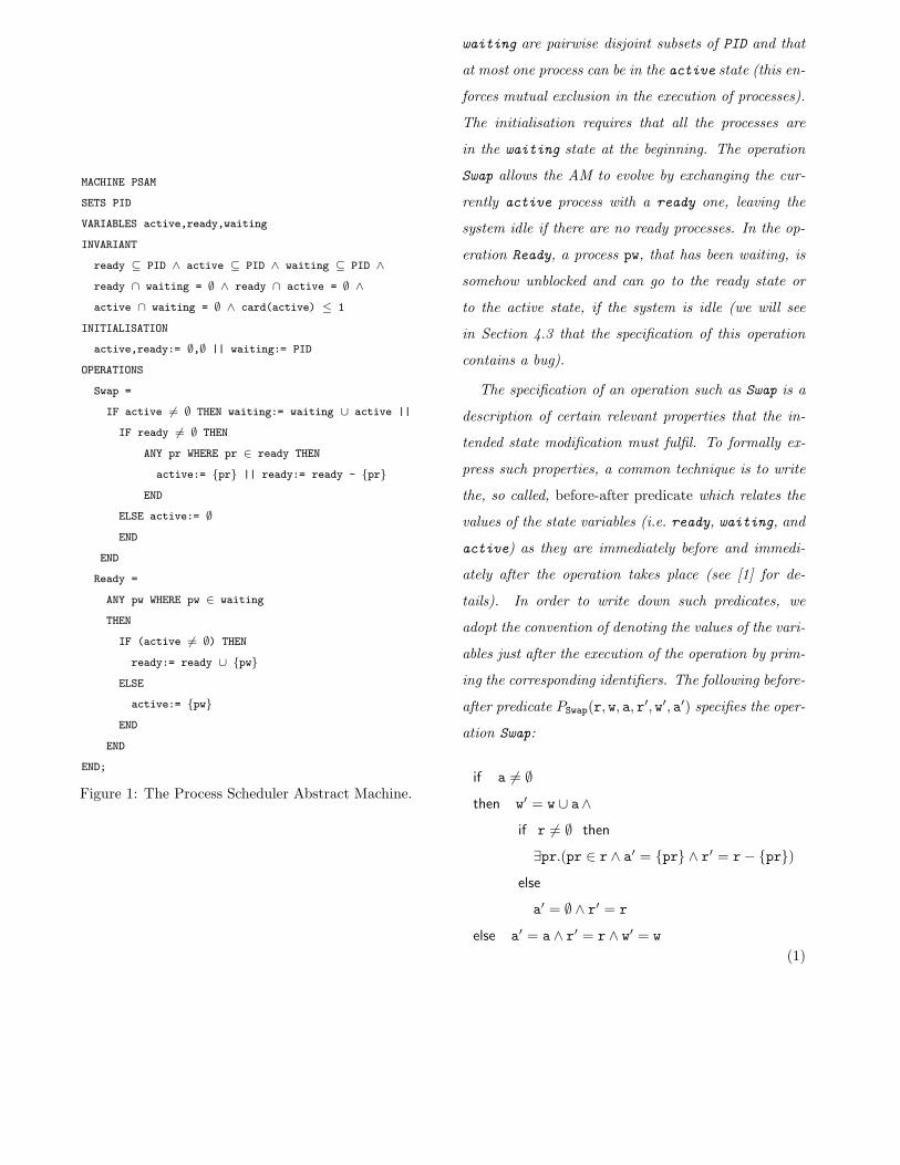
Example 1 (The Process Scheduler) As a running

example on which we illustrate our techniques, we con-

sider the process scheduler introduced in [11]. Although

simple, this example allows us to discuss the typical

problems arising in handling the type of AMs our tech-

nique is aimed at, i.e. (large) AMs which manipulate

simple data structures, represented by sets of primitive

elements. Its B specification is shown in Figure 1. At

any one time, the system may have some processes

ready to be scheduled, some processes waiting for

some external action before they become ready and,

possibly, a single active process. Each process is

uniquely identified by an identifier (taken out of a set

PID). The invariant states that active, ready, and

MACHINE PSAM

SETS PID

VARIABLES active,ready,waiting

INVARIANT

ready ⊆ PID ∧ active ⊆ PID ∧ waiting ⊆ PID ∧

ready ∩ waiting = ∅ ∧ ready ∩ active = ∅ ∧

active ∩ waiting = ∅ ∧ card(active) ≤ 1

INITIALISATION

active,ready:= ∅,∅ || waiting:= PID

OPERATIONS

Swap =

IF active 6= ∅ THEN waiting:= waiting ∪ active ||

IF ready 6= ∅ THEN

ANY pr WHERE pr ∈ ready THEN

active:= {pr} || ready:= ready - {pr}

END

ELSE active:= ∅

END

END

Ready =

ANY pw WHERE pw ∈ waiting

THEN

IF (active 6= ∅) THEN

ready:= ready ∪ {pw}

ELSE

active:= {pw}

END

END

END;

Figure 1: The Process Scheduler Abstract Machine.

waiting are pairwise disjoint subsets of PID and that

at most one process can be in the active state (this en-

forces mutual exclusion in the execution of processes).

The initialisation requires that all the processes are

in the waiting state at the beginning. The operation

Swap allows the AM to evolve by exchanging the cur-

rently active process with a ready one, leaving the

system idle if there are no ready processes. In the op-

eration Ready, a process pw, that has been waiting, is

somehow unblocked and can go to the ready state or

to the active state, if the system is idle (we will see

in Section 4.3 that the specification of this operation

contains a bug).

The specification of an operation such as Swap is a

description of certain relevant properties that the in-

tended state modification must fulfil. To formally ex-

press such properties, a common technique is to write

the, so called, before-after predicate which relates the

values of the state variables (i.e. ready, waiting, and

active) as they are immediately before and immedi-

ately after the operation takes place (see [1] for de-

tails). In order to write down such predicates, we

adopt the convention of denoting the values of the vari-

ables just after the execution of the operation by prim-

ing the corresponding identifiers. The following before-

after predicate PSwap(r, w, a, r′, w′, a′) specifies the oper-

ation Swap:

if a 6= ∅then w′ = w ∪ a∧

if r 6= ∅ then

∃pr.(pr ∈ r ∧ a′ = {pr} ∧ r′ = r− {pr})else

a′ = ∅ ∧ r′ = r

else a′ = a ∧ r′ = r ∧ w′ = w

(1)

where r, w, a, r′, w′, a′ abbreviate ready, waiting,

active, ready′, waiting′ and active′ respectively.

The Boolean conditional connective if A then B else

C abbreviates (A ⇒ B) ∧ (¬A ⇒ C) where

A,B, and C are formulae. We use such a construct

in order to preserve the structure of the B specifi-

cation in the before-after predicate. Notice that the

non-deterministic choice operator (ANY) is expressed

by existential quantification and the multiple assign-

ment operator (||) by conjunction. Also, state vari-

ables that are not explicitly assigned retain their pre-

vious value. Although this is not in the scope of this

paper, we believe it would be easy to adapt our ap-

proach to handle other B constructs such as constants,

machine parameters and properties.

The invariant (cf. INVARIANT clause of Figure 1)

can easily be translated to the following predicate:

r ⊆ p ∧ w ⊆ p ∧ a ⊆ p∧r ∩ w = ∅ ∧ r ∩ a = ∅ ∧ a ∩ w = ∅∧card(a) ≤ 1,

(2)

where p is a constant representing PID; it is abbrevi-

ated by Inv(r, w, a).

Once both an operation and the invariant have been

specified by predicates, we can prove that the operation

preserves the invariant by checking the validity of the

following formula which encodes the fact that Inv holds

after the execution of Swap, provided that it holds be-

fore:

∀r, w, a, r′, w′, a′. [Inv(r, w, a) ∧ PSwap(r, w, a, r′, w′, a′)

⇒ Inv(r′, w′, a′)].

(3)

In addition to proving that each operation pre-

serves the invariant Inv, one also has to check that

Inv is satisfied by the initialisation condition (cf.

INITIALISATION clause of Figure 1). We omit the

corresponding proof obligation, since this does not add

much to the discussion.

Proof obligations—such as (3)— shall be discharged

by using automated theorem provers. Typically, in

currently available commercial tools supporting the B

method, there is a number of proof obligations that

the automated prover cannot discharge so the devel-

oper can switch the prover to an interactive mode and

attempt to try to discharge the remaining proof obliga-

tions manually. The B method is actually supported

by two commercially available tools: the B-Toolkit4

and the AtelierB.5 Although quite successful, both

tools leave the developer without help to discover why

a certain proof obligation has failed to be shown valid.

In the rest of this paper, we describe a technique

to check the validity of proof obligations and to pro-

vide the user with counter-examples when the validity

check fails.

3 Translating Set-Based Proof Obliga-

tions

In Section 2, we have relied on the reader’s intu-

ition of basic concepts of first-order logic and naive

set theory to write down the before-after predicates

specifying the operation, the invariant, and the proof

obligation of the AM in Figure 1. Here, we define the

simple version of set theory we use and explain how

to translate it into a suitable extension of first-order

logic with equality so that haRVey (cf. Section 4.2)—a

system to check the validity of equational first-order

4http://www.b-core.com/btoolkit.html5http://www.atelierb.societe.com/index.html

formulae—can be used to discharge such proof obliga-

tions (if possible).

Below, we assume the usual syntactic and semantic

notions of first-order logic with equality as defined for

example in [12]. We say that a formula φ is satisfiable

modulo a theory T iff φ ∧ T is satisfiable.6

3.1 A Simple Set Theory

For simplicity, in this paper, we consider a re-

stricted fragment of set theory, which we denote with

SSET . Notice, however, that our approach can be

extended to handle more expressive fragments of set

theory such as the theory of Hereditarily Finite Sets

with Atoms (see, e.g. [5]), which permits sets of prim-

itive elements, sets of sets of primitive elements, and

so on. SSET is a theory of first-order sorted logic with

equality. It contains two distinct sort symbols elem

and set. Its set of terms contains the variable and

constant symbols of sort elem and set. We assume

there is at least one constant of sort elem. The distin-

guished constant ∅ is a term of sort set. If e is a term

of sort elem, then {e} is a term of sort set; also, if

s1 and s2 are terms of sort set, then s1 ./ s2 is also a

term of sort set, where ./ is one of the binary function

symbols ∩ (intersection), ∪ (union), and \ (set differ-

ence). We also write {e1, . . . , en} as an abbreviation

of {e1} ∪ · · · ∪ {en}. The set of atoms of SSET con-

tains expressions of the form e1 = e2, e ∈ s, s1 ⊆ s2,

s1 = s2, where e, e1, e2 are terms of sort elem and

s, s1, s2 are terms of sort set. Literals, Boolean com-

binations of literals, and possibly quantified formulae

are inductively defined in the usual way. Furthermore,

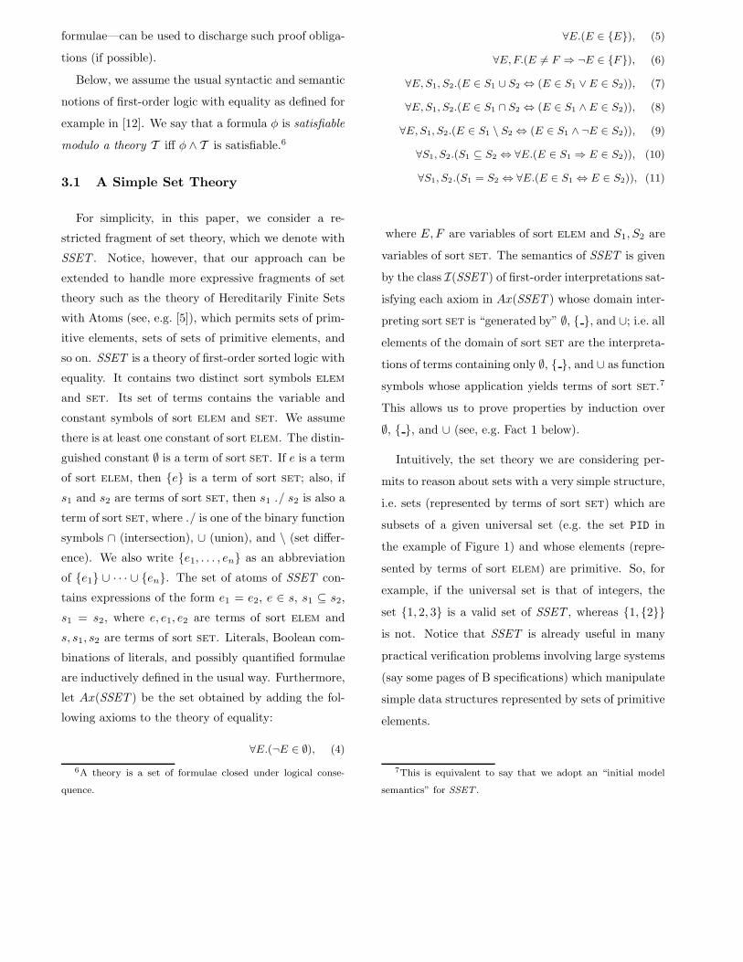
let Ax(SSET ) be the set obtained by adding the fol-

lowing axioms to the theory of equality:

∀E.(¬E ∈ ∅), (4)

6A theory is a set of formulae closed under logical conse-

quence.

∀E.(E ∈ {E}), (5)

∀E,F.(E 6= F ⇒ ¬E ∈ {F}), (6)

∀E, S1, S2.(E ∈ S1 ∪ S2 ⇔ (E ∈ S1 ∨E ∈ S2)), (7)

∀E, S1, S2.(E ∈ S1 ∩ S2 ⇔ (E ∈ S1 ∧E ∈ S2)), (8)

∀E, S1, S2.(E ∈ S1 \ S2 ⇔ (E ∈ S1 ∧ ¬E ∈ S2)), (9)

∀S1, S2.(S1 ⊆ S2 ⇔ ∀E.(E ∈ S1 ⇒ E ∈ S2)), (10)

∀S1, S2.(S1 = S2 ⇔ ∀E.(E ∈ S1 ⇔ E ∈ S2)), (11)

where E,F are variables of sort elem and S1, S2 are

variables of sort set. The semantics of SSET is given

by the class I(SSET ) of first-order interpretations sat-

isfying each axiom in Ax(SSET ) whose domain inter-

preting sort set is “generated by” ∅, { }, and ∪; i.e. all

elements of the domain of sort set are the interpreta-

tions of terms containing only ∅, { }, and ∪ as function

symbols whose application yields terms of sort set.7

This allows us to prove properties by induction over

∅, { }, and ∪ (see, e.g. Fact 1 below).

Intuitively, the set theory we are considering per-

mits to reason about sets with a very simple structure,

i.e. sets (represented by terms of sort set) which are

subsets of a given universal set (e.g. the set PID in

the example of Figure 1) and whose elements (repre-

sented by terms of sort elem) are primitive. So, for

example, if the universal set is that of integers, the

set {1, 2, 3} is a valid set of SSET , whereas {1, {2}}is not. Notice that SSET is already useful in many

practical verification problems involving large systems

(say some pages of B specifications) which manipulate

simple data structures represented by sets of primitive

elements.

7This is equivalent to say that we adopt an “initial model

semantics” for SSET .

3.2 The Theory of Arrays with Extension-

ality

Let Aes be the many-sorted theory with sorts value,

index and array, with function symbols write (ab-

breviated below with wr) and read (abbreviated below

with rd) of type array × index × value −→ array

and array× index −→ value respectively. Further-

more, let Ax(Aes) be the set of axioms obtained by

adding the following axioms to the theory of equality:

∀A, I,E.(rd(wr(A, I,E), I) = E), (12)

∀A, I, J, E.(I 6= J ⇒ rd(wr(A, I,E), J) = rd(A, J)), (13)

∀A,B.(∀I.(rd(A, I) = rd(B, I))⇒ A = B), (14)

where A and B are variables of sort array, I and

J are variables of sort index, and E is a variable of

sort value. ΣAes

denotes a signature containing the

function symbols rd, wr, and a finite set of constant

symbols. We assume that the signature of Aes admits

at least one ground term for each sort. Checking the

satisfiability of conjunctions of ground literals modulo

Aes is decidable (see, e.g. [3]).

3.3 From Set Theory to Array Theory

We explain how to translate formulae of SSET to

(extensions of) Aes so that the reasoning system haR-

Vey (cf. Section 4.2) can be used to discharge the proof

obligations which imply that an invariant of an AM is

an inductive property of the machine (along the lines

sketched in Section 2).

The intuition underlying our approach is based

on using the characteristic function to represent sets.

Such a function, in turn, can be encoded by an array

of Booleans whose indexes are the elements of the set.

For example, the set s := {1, 2} can be represented as

s[1] = s[2] = true and s[x] = false, for all x distinct

from 1 and 2.

First, let BAes ⊃ Aes be an extension of Ae

s contain-

ing two distinguished constants tt and ff of sort value

together with the axiom

tt 6= ff. (15)

In this way, we consider arrays storing Boolean values

(from this, the ‘B’ in front of ‘Aes’ in ‘BAe

s’). Further-

more, BAes contains a distinguished constant symbol

mty of sort array and the axiom

∀I.(rd(mty, I) = ff), (16)

where I is a variable of sort index (the intuition is

that mty is the counterpart of the empty set in Aes).

Then, we define three functions S, T, and F from the

sorts, terms, and formulae of SSET to the sorts, pairs

of terms and set of formulae, and pairs of formulae

and set of formulae (respectively) of BAes. Below, we

will see that other symbols and axioms will be added to

BAes in the process of translating a formula of SSET to

a formula in first-order logic with equality by applying

functions T and F. Formally, this is done by returning

the translated terms together with the set of formulae

to be added to BAes. Such formulae will implicitely

determine the symbols to be added to BAes.

We define S(elem) := index and S(set) :=

array. Then, we assume that T is s.t. it maps (one-

to-one) constants of sort elem and set to constants of

sort index and array, respectively. Now, we home-

omorphically extend T to compound terms of SSET

as follows, where i and u are fresh constants of sort

index and array, respectively:

T(∅) := (mty, ∅);T(x) := (i, ∅) if x is of sort elem;

T(x) := (u, ∅) if x is of sort set;

T({e}) := (u, {u = wr(mty, e, tt)}),

T(e1 ∪ e2) := (u, {a∪} ∪ α1 ∪ α2),

T(e1 ∩ e2) := (u, {a∩} ∪ α1 ∪ α2), and

T(e1 \ e2) := (u, {a\} ∪ α1 ∪ α2), where

a∪ is ∀I.(rd(e1, I) = tt∨rd(e2, I) = tt ⇔ rd(u, I) = tt),

a∩ is ∀I.(rd(e1, I) = tt∧rd(e2, I) = tt ⇔ rd(u, I) = tt),

a\ is ∀I.(rd(e1, I) = tt ∧ rd(e2, I) = ff ⇔ rd(u, I) =

tt) and T(ej) = (ej , αj) for j = 1, 2. We re-

gard {e1, ..., en} (for n > 1) as an abbreviation of

{e1} ∪ · · · ∪ {en}.Then, for each constant u of sort array (represent-

ing a set), we add to BAes the following axiom:

∀I.(rd(u, I) = tt ∨ rd(u, I) = ff), (17)

where I is a variable of sort index. Axiom (17) con-

strains the co-domain of the characteristic function

represented by u to be {tt,ff}.Furthermore, we translate the ground atoms of

SSET by defining the function F as follows:

F(e1 ∈ e2) := (rd(e2, e1) = tt, α1 ∪ α2),

F(e1 = e2) := (e1 = e2, α1 ∪ α2),

F(e1 6= e2) := F(¬(e1 = e2)),

F(e1 ⊂ e2) := F(e1 ⊆ e2 ∧ e1 6= e2),

F(e1 ⊆ e2) := (q, α1 ∪ α2 ∪ α),

where q is a fresh propositional letter, T(ei) = (ei, αi)

for i = 1, 2 and α is {q ⇔ ∀X.(rd(e1, X) = tt ⇒rd(e2, X) = tt)}.

Then, the translation process is homeomorphically

extended to Boolean combinations of atoms in the fol-

lowing way:

F(¬φ) := (¬ φ, α) where F(φ) = (φ, α),

F(φ1 � φ2) := (φ1 � φ2, α1 ∪ α2)

where F(φi) = (φi, αi) for i = 1, 2 and � stands for

either ∨,∧,⇒ or ⇔, and

F(if φ1 then φ2 else φ3) := (if φ1 then φ2 else φ3,

α1 ∪ α2 ∪ α3)

where F(φi) = (φi, αi) for i = 1, 2, and 3.

Now, we are in the position to state the main prop-

erty of our translation process (we state it in terms

of satisfiability since our theorem proving approach

is based on refutation; see Section 4.2). Let φ be

a ground formula of SSET and (φ, α) = F(φ) be its

translation. We denote by BAes the theory containing

Aes, the axioms (15), (16), (17) and the formulae in α.

Theorem 1 φ is satisfiable modulo SSET iff φ is sat-

isfiable modulo BAes.

In order to prove the Theorem, we need some technical

definitions and facts.

Fact 1 For any ground term t of SSET, there exists

a term t′ containing only the function symbols ∅, { },and ∪ s.t. t = t′ is satisfied by an interpretation in

I(SSET ).

The proof consists of an easy induction on ∅, { }, and

∪. Then, we introduce the function ins as follows:

ins(e, ∅) = {e} (18)

ins(e, s) = {e} ∪ s, (19)

for all ground terms e and s of sort elem and set,

respectively.

Fact 2 Let R be the term rewriting system consist-

ing of (18) and (19), oriented from right to left, and

ins(e,mty) ∪ s = ins(e, s), oriented from left to right.

Then, R is terminating and confluent.

The termination of R can be easily seen by observing

that the number of occurrences of { } and ∪ decreases

following the orientation of each rewrite rule. It is

also trivial to see that if a term t does not contain

any occurrence of { } or ∪, then no rule in R can be

applied. The fact of being confluent is an immedi-

ate consequence of the fact that the set of equations

is closed under the rules of the superposition calculus

[16].8 As a consequence, we are entitled to define a

function ·′ on terms of SSET obtained by using Facts

1 and 2. By abuse of notation, we extend such a func-

tion to formulae as follows: φ′ will denote the formula

obtained from φ by applying ·′ to its sub-terms. Then,

we introduce the set Ax(SSET ′) of axioms obtained

from Ax(SSET ) by replacing (5) and (6) with

∀E, S.(E ∈ ins(E, S)), (20)

∀E,F, S.(E 6= F ⇒ (E ∈ ins(F, S) ⇔ E ∈ S)), (21)

where E,F are variables of sort elem and S is a vari-

able of sort set. The signature of SSET ′ is obtained

from that of SSET by replacing { } with ins.

Fact 3 φ is SSET-satisfiable iff φ′ is SSET ′-

satisfiable.

To see this, it is sufficient to observe that both (20)

and (21) are logical consequences of Ax(SSET ) and

of (18) and (19). Now, we consider the mapping T′

from ground terms of SSET ′ to pairs of ground terms

and set of formulae of BAes defined as follows, where

i and u are fresh constants of sort index and array,

respectively:

T′(ins(e, s)) := (wr(s, e, tt), α) where T′(s) = (s, α);

T′(∅) := (mty, ∅);T′(x) := (i, ∅) if x is of sort elem;

T′(x) := (u, au) if x is of sort set, where au is

∀I.(rd(u, I) = tt ∨ rd(u, I) = ff), and I is a variable of

sort index;

T′(e1 ∪ e2) := (u, {a∪} ∪ α1 ∪ α2), where

8In fact, ins(e,mty)∪s = ins(e, s) is obtained by superposition

of (18) and (19).

a∪ is ∀I.(rd(e1, I) = tt∨ rd(e2, I) = tt ⇔ rd(u, I) = tt)

and T′(ej) = (ej , αj) for j = 1, 2.

Lemma 1 Let t be a ground term on the signature of

SSET and t′ be the translated term on the signature of

SSET ′. Let T(t) = (s, α) and T′(t′) = (s′, α′). Then,

s = s′ is a logical consequence of Aes, α, α′, (15), (16)

and (17).

Again, the proof is obtained by induction on the struc-

ture of the term t and therefore is omitted. If we define

F′ as F above where the calls to T are replaced with

calls to T′, then we can easily derive that ψ is logically

equivalent to ψ′ modulo Aes ∪ {α, α′} as a corollary of

Lemma 1, where (ψ, α) = F(φ) and (ψ′, α′) = F(φ′).

The following diagram summarizes the situation:

SSET SSET ′

BAes

·′

F F′

Proof of Theorem 1. We prove (the counterposi-

tive of) if φ is satisfiable modulo SSET then φ is satisfi-

able modulo BAes. First of all, we translate the formula

φ of SSET to a formula φ′ of SSET ′ by using Fact 1

and Fact 2. Then, we observe that the translation of

the ground instances of the axioms in Ax(SSET ′) (un-

der F′) are all logical consequences of Ax(BAes). If φ′

is the formula of BAes which is the translation of φ′

under F′, then, by Fact 3, Lemma 1, and the previ-

ous observation, we are entitled to conclude that φ is

unsatisfiable modulo SSET if φ is unsatisfiable mod-

ulo BAes. The other implication of the biconditional is

similar and therefore omitted. 2

3.4 Two Important Extensions

In order to enlarge the scope of applicability of our

technique, we consider two extensions of the transla-

tion defined above. The former handles (a restricted

form of) the cardinality operator which is frequently

used in set-based specification. The latter considers

non-ground formulae containing quantifiers over the

elements of the universal set. We do not consider

quantifiers over sets since it is well-known that the

full first-order theory of arrays is undecidable (see [3]

for further references on this point).

The cardinality operator. Let us consider only

ground atoms of the form card(s) = k, where s is a

term of sort set and k is a given numeral. Then,

we can replace each atom of the form card(s) =

k with s = {f1, ..., fk}, where fi is a fresh con-

stant of sort elem (for i = 1, ..., k). After the

exhaustive application of such a rule we obtain a

formula of SSET which can be translated to BAes

as described above. We can generalise the ap-

proach to handle more complex arithmetic relation.

For example, card(active) ≤ 1 can be rewritten as

card(active) = 0 ∨ card(active) = 1 which, in turn,

rewrites to active = ∅ ∨ active = {f1}, where f1 is a

fresh constant of sort elem. Formally, we extend the

definition of F above as follows:

F(card(e) = 0) := (e = mty, α)

where T(e) = (e, α),

F(card(e) = k) := (q, α ∪ {q ⇔ ∃x1, · · · , xk.β})

F(card(e) ≤ k) := (q, α ∪ {q ⇔ ∃x1, · · · , xk.ϕ})

where q is a fresh propositional letter, k is a numeral

constant denoting an integer s.t. k 6= 0, T(e) = (e, α),

ϕ is e = wr(· · ·wr(mty, x1, tt) · · · , xk, tt), and β is∧

1≤i<j≤k (xi 6= xj) ∧ ϕ.

By applying the above three equations defining the

extension of F, we can eliminate all occurrences of the

cardinality operator in a formula. As a consequence,

we obtain a formula of SSET to which Theorem 1 is

still applicable. In other words, Theorem 1 can be

straightforwardly adapted to hold for the extension

of SSET with the restricted form of the cardinality

operator considered here.

Quantifiers over set elements. Frequently, the

proof obligations resulting from the verification of in-

variants of B machines are not ground. They usu-

ally contain quantifiers over the elements of a cer-

tain set. For example, we will obtain existentially

quantified sub-formulae whenever we handle the non-

deterministic choice operator (i.e. ANY), see the Exam-

ple below. To handle quantifiers over elements of sets,

we define the function FQ to be equal to F on ground

formulae and s.t.

FQ(Qx.φ) := (Qx.φ, α)

where x is a variable of sort elem, Q is either ∀ or ∃,

and FQ(φ) = (φ, α).

Example 2 (The Process Scheduler—continued)

The before-after predicate PSwap in (1) is translated to

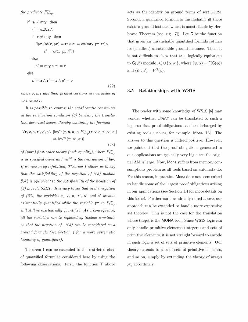
the predicate P eqSwap:

if a 6= mty then

w′ = w U a∧if r 6= mty then

∃pr.(rd(r, pr) = tt ∧ a′ = wr(mty, pr, tt)∧r′ = wr(r, pr,ff))

else

a′ = mty ∧ r′ = r

else

a′ = a ∧ r′ = r ∧ w′ = w

(22)

where w, a, r and their primed versions are variables of

sort array.

It is possible to express the set-theoretic constructs

in the verification condition (3) by using the transla-

tion described above, thereby obtaining the formula

∀r, w, a, r′, w′, a′. [Inveq(r, w, a) ∧ P eqSwap(r, w, a, r′, w′, a′)⇒ Inveq(r′, w′, a′)]

(23)

of (pure) first-order theory (with equality), where P eqSwap

is as specified above and Inveq is the translation of Inv.

If we reason by refutation, Theorem 1 allows us to say

that the satisfiability of the negation of (23) modulo

BAes is equivalent to the satisfiability of the negation of

(3) modulo SSET. It is easy to see that in the negation

of (23), the variables r, w, a, r′, w′ and a′ become

existentially quantified while the variable pr in P eqSwap

will still be existentially quantified. As a consequence,

all the variables can be replaced by Skolem constants

so that the negation of (23) can be considered as a

ground formula (see Section 4 for a more systematic

handling of quantifiers).

Theorem 1 can be extended to the restricted class

of quantified formulae considered here by using the

following observations. First, the function T above

acts as the identity on ground terms of sort elem.

Second, a quantified formula is unsatisfiable iff there

exists a ground instance which is unsatisfiable by Her-

brand Theorem (see, e.g. [7]). Let G be the function

that given an unsatisfiable quantified formula returns

its (smallest) unsatisfiable ground instance. Then, it

is not difficult to show that ψ is logically equivalent

to G(ψ′) modulo Aes ∪{α, α′}, where (ψ, α) = F(G(φ))

and (ψ′, α′) = FQ(φ).

3.5 Relationships with WS1S

The reader with some knowledge of WS1S [6] may

wonder whether SSET can be translated to such a

logic so that proof obligations can be discharged by

existing tools such as, for example, Mona [13]. The

answer to this question is indeed positive. However,

we point out that the proof obligations generated in

our applications are typically very big since the origi-

nal AM is large. Now, Mona suffers from memory con-

sumptions problem as all tools based on automata do.

For this reason, in practice, Mona does not seem suited

to handle some of the largest proof obligations arising

in our applications (see Section 4.4 for more details on

this issue). Furthermore, as already noted above, our

approach can be extended to handle more expressive

set theories. This is not the case for the translation

whose target is the MONA tool. Since WS1S logic can

only handle primitive elements (integers) and sets of

primitive elements, it is not straightforward to encode

in such logic a set of sets of primitive elements. Our

theory extends to sets of sets of primitive elements,

and so on, simply by extending the theory of arrays

Aes accordingly.

4 Discharging Proof Obligations

We are left with the problem of checking that for-

mulae of first-order logic with equality, such as (23),

are logical consequences of the equational theory BAes.

To do this, we reason by refutation and prove that the

negation of the formula is unsatisfiable modulo BAes.

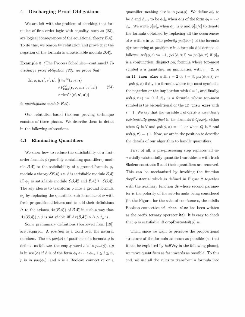
Example 3 (The Process Scheduler—continued) To

discharge proof obligation (23), we prove that

∃r, w, a, r′, w′, a′. [(Inveq(r, w, a)

∧P eqSwap(r, w, a, r′, w′, a′)∧¬Inveq(r′, w′, a′)]

(24)

is unsatisfiable modulo BAes.

Our refutation-based theorem proving technique

consists of three phases. We describe them in detail

in the following subsections.

4.1 Eliminating Quantifiers

We show how to reduce the satisfiability of a first-

order formula φ (possibly containing quantifiers) mod-

ulo BAes to the satisfiability of a ground formula φg

modulo a theory EBAes s.t. φ is satisfiable modulo BAe

s

iff φg is satisfiable modulo EBAes and BAes ⊆ EBAe

s.

The key idea is to transform φ into a ground formula

φg by replacing the quantified sub-formulae of φ with

fresh propositional letters and to add their definitions

∆ to the axioms Ax(BAes) of BAes in such a way that

Ax(BAes) ∧ φ is satisfiable iff Ax(BAe

s) ∧ ∆ ∧ φg is.

Some preliminary definitions (borrowed from [19])

are required. A position is a word over the natural

numbers. The set pos(φ) of positions of a formula φ is

defined as follows: the empty word ε is in pos(φ), i.p

is in pos(φ) if φ is of the form φ1 ◦ · · · ◦ φn, 1 ≤ i ≤ n,

p is in pos(φi), and ◦ is a Boolean connective or a

quantifier; nothing else is in pos(φ). We define φ|ε to

be φ and φ|i.p to be φi|p when φ is of the form φ1 ◦· · ·◦φn. We write φ[ψ]p when φ|p is ψ and φ[x/c] to denote

the formula obtained by replacing all the occurrences

of x with c in φ. The polarity pol(φ, π) of the formula

φ|π occurring at position π in a formula φ is defined as

follows: pol(φ, ε) := +1, pol(φ, π.i) := pol(φ, π) if φ|πis a conjunction, disjunction, formula whose top-most

symbol is a quantifier, an implication with i = 2, or

an if then else with i = 2 or i = 3, pol(φ, π.i) :=

−pol(φ, π) if φ|π is a formula whose top-most symbol is

the negation or the implication with i = 1, and finally,

pol(φ, π.i) := 0 if φ|π is a formula whose top-most

symbol is the biconditional or the if then else with

i = 1. We say that the variable x of Qx.ψ is essentially

existentially quantified in the formula φ[Qx.ψ]π either

when Q is ∀ and pol(φ, π) = −1 or when Q is ∃ and

pol(φ, π) = +1. Now, we are in the position to describe

the details of our algorithm to handle quantifiers.

First of all, a pre-processing step replaces all es-

sentially existentially quantified variables a with fresh

Skolem constants a and their quantifiers are removed.

This can be mechanised by invoking the function

dropExistential which is defined in Figure 2 together

with the auxiliary function de whose second parame-

ter is the polarity of the sub-formula being considered

(in the Figure, for the sake of conciseness, the mixfix

Boolean connective if then else has been written

as the prefix ternary operator ite). It is easy to check

that φ is satisfiable iff dropExistential(φ) is.

Then, since we want to preserve the propositional

structure of the formula as much as possible (so that

it can be exploited by haRVey in the following phase),

we move quantifiers as far inwards as possible. To this

end, we use all the rules to transform a formula into

dropExistential(φ) := de(φ,+1)

de(φ, p) := φ if φ is atomic,

de(¬φ, p) := ¬de(φ,−p)

de(φ ∧ ψ, p) := de(φ, p) ∧ de(ψ, p)

de(φ ∨ ψ, p) := de(φ, p) ∨ de(ψ, p)

de(ite(φ,ψ, ξ), p) := ite(φ, de(ψ, p), de(ξ, p))

de(φ ⇒ ψ, p) := de(φ,−p) ⇒ de(ψ, p)

de(φ ⇔ ψ, p) := φ ⇔ ψ

de(∀x.φ,+1) := ∀x.φ

de(∃x.φ,−1) := ∃x.φ

de(∀x.φ,−1) := de(φ[x/c],+1)

de(∃x.φ,+1) := de(φ[x/c],−1)

Figure 2: Definition of dropExistential and de.

prenex form9 (see again [12] for details) but in the op-

posite direction. For example, the formula ∃x.(φ ⇒ ψ)

is transformed to (∀x.φ) ⇒ ψ if x does not occur in ψ.

This operation, known as miniscoping, can be mech-

anised as shown in Figure 3. We assume that only

formulae obtained as the result of the invocation of

dropExistential are fed to mini. The function is de-

fined on the structure of first-order formulae. When

it encounters an atomic formula it simply returns it

whereas when a quantified sub-formula is met, the

auxiliary function mq is invoked. In the definition of

mq , the following notation is used: Q abbreviates ei-

ther ∀ or ∃, −Q abbreviates ∀ (∃) when Q is ∃ (∀),

V(φ) denotes the set of free variables in φ and x′ is a

fresh variable. The first and the second arguments of

mq are the quantifier and the quantified variable whose

scope is reduced by the function while the third argu-

ment is the already processed sub-formula. Again, it

9A formula is in prenex form if it has the structure

Q1x1...Qnxn.φ, where Qi is either ∀ or ∃, xi is a variable

(i = 1, ..., n), and φ is a quantifier-free formula whose free vari-

ables are x1, ..., xn.

mini(φ ◦ ψ) := mini(φ) ◦ mini(ψ) where ◦ ∈ {∧,∨,⇒,⇔}

mini(¬φ) := ¬mini(φ)

mini(ite(φ,ψ, ξ)) := ite(mini(φ),mini(ψ),mini(ξ))

mini(φ) := φ if φ is atomic

mini(Q x1, · · · , xn.φ) := mq(Q,x1, . . .mq(Q,xn,mini(φ)) . . .)

mq(Q,x, φ) := φ if x 6∈ V(φ)

mq(Q, x,¬φ) := ¬mq(−Q,x, φ)

mq(Q,x, φ � ψ) := mq(Q,x, φ) � ψ if x 6∈ V(ψ), � ∈ {∧,∨}

mq(Q,x, φ � ψ) := φ � mq(Q, x,ψ) if x 6∈ V(φ), � ∈ {∧,∨}

mq(∀, x, φ ∧ ψ) := mq(∀, x, φ) ∧ mq(∀, x′

, ψ[x/x′

]) otherwise

mq(∃, x, φ ∨ ψ) := mq(∃, x, φ) ∨ mq(∃, x′, ψ[x/x′]) otherwise

mq(Q,x, φ ⇒ ψ) := φ ⇒ mq(Q,x, ψ) if x 6∈ V(φ)

mq(Q,x, φ ⇒ ψ) := mq(−Q,x, φ) ⇒ ψ if x 6∈ V(ψ)

mq(∃, x, φ ⇒ ψ) := mq(∀, x, φ) ⇒ mq(∃, x′, ψ[x/x′])

mq(Q, x, ite(φ,ψ, ξ)) := ite(φ,ψ,mq(Q,x, ξ)) if x 6∈ V(φ) ∪ V(ψ)

mq(Q, x, ite(φ,ψ, ξ)) := ite(φ,mq(Q, x,ψ), ξ) if x 6∈ V(φ) ∪ V(ξ)

mq(Q,x, φ) := Q x.φ otherwise

Figure 3: Definition of mini and mq .

is a routine exercise to check that φ is satisfiable iff

mini(φ) is.

As the third and last step, we replace each out-

ermost quantified sub-formula ψ with a fresh propo-

sitional letter q and we add q ⇒ ψ (resp. ψ ⇒ q,

q ⇔ ψ) to Ax(BAes) if φ|π = ψ and pol(φ, π) = +1

(resp. pol(φ, π) = −1, pol(φ, π) = 0). Notice that

if there is a quantified sub-formula ψ′ occurring in

ψ, we do not recursively apply the above process to

ψ′ but we stop at ψ. This is a heuristic decision

which seems to give good results in practice. The

mechanization of this last phase is given in Figure

4. We assume that only formulae obtained from the

applications of dropExistential first followed by mini

are passed to renameFormula. The first argument of

the auxiliary function rf is the formula being con-

sidered and the second is its polarity. The function

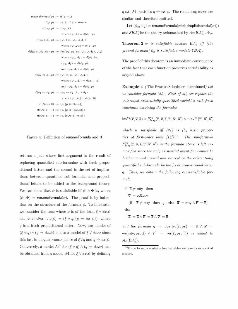
renameFormula(φ) := rf(φ,+1)

rf(φ, p) := (φ, ∅) if φ is atomic

rf(¬φ, p) := (¬ψ,A)

where (ψ,A) = rf(φ,−p)

rf(φ1 � φ2, p) := (ψ1 � ψ2,A1 ∪ A2)

where (ψi,Ai) = rf(φi, p)

rf(ite(φ1, φ2, φ3), p) := (ite(ψ1, ψ2, ψ3),A1 ∪ A2 ∪ A3)

where (ψ1,A1) = rf(φ1, 0),

(ψ2,A2) = rf(φ2, p)

and (ψ3,A3) = rf(φ3, p)

rf(φ1 ⇒ φ2, p) := (ψ1 ⇒ ψ2,A1 ∪ A2)

where (ψ1,A1) = rf(φ1,−p)

and (ψ2,A2) = rf(φ2, p)

rf(φ1 ⇔ φ2, p) := (ψ1 ⇔ ψ2,A1 ∪ A2)

where (ψi,Ai) = rf(φi, 0)

rf(Qx.φ, 0) := (p, {p ⇔ Qx.φ})

rf(Qx.φ,+1) := (p, {p ⇒ (Qx.φ)})

rf(Qx.φ,−1) := (p, {(Qx.φ) ⇒ p})

Figure 4: Definition of renameFormula and rf .

returns a pair whose first argument is the result of

replacing quantified sub-formulae with fresh propo-

sitional letters and the second is the set of implica-

tions between quantified sub-formulae and proposi-

tional letters to be added to the background theory.

We can show that φ is satisfiable iff φ′ ∧ Φ is, where

(φ′,Φ) = renameFormula(φ). The proof is by induc-

tion on the structure of the formula φ. To illustrate,

we consider the case where φ is of the form ξ ∨ ∃x.ψs.t. renameFormula(φ) = (ξ ∨ q, {q ⇒ ∃x.ψ}), where

q is a fresh propositional letter. Now, any model of

(ξ ∨ q) ∧ (q ⇒ ∃x.ψ) is also a model of ξ ∨ ∃x.ψ since

this last is a logical consequence of ξ∨q and q ⇒ ∃x.ψ.

Conversely, a model M′ for (ξ ∨ q) ∧ (q ⇒ ∃x.ψ) can

be obtained from a model M for ξ ∨ ∃x.ψ by defining

q s.t. M′ satisfies q ⇔ ∃x.ψ. The remaining cases are

similar and therefore omitted.

Let (φg ,Φg) = renameFormula(mini(dropExistential(φ)))

and EBAes be the theory axiomatized by Ax(BAe

s)∪Φg .

Theorem 2 φ is satisfiable modulo BAes iff (the

ground formula) φg is satisfiable modulo EBAes.

The proof of this theorem is an immediate consequence

of the fact that each function preserves satisfiability as

argued above.

Example 4 (The Process Scheduler—continued) Let

us consider formula (24). First of all, we replace the

outermost existentially quantified variables with fresh

constants obtaining the formula:

Inveq(r, w, a) ∧ P eqSwap(r, w, a, r′, w′, a′) ∧ ¬Inveq(r′, w′, a′).

which is satisfiable iff (24) is (by basic proper-

ties of first-order logic [12]).10 The sub-formula

P eqSwap(r, w, a, r′, w′, a′) in the formula above is left un-

modified since the only existential quantifier cannot be

further moved inward and we replace the existentially

quantified sub-formula by the fresh propositional letter

q. Thus, we obtain the following equisatisfiable for-

mula

if a 6= mty then

w′ = w U a∧(if r 6= mty then q else a′ = mty ∧ r′ = r)

else

a′ = a ∧ r′ = r ∧ w′ = w

and the formula q ⇒ ∃pr.(rd(r, pr) = tt ∧ a′ =

wr(mty, pr, tt) ∧ r′ = wr(r, pr,ff)) is added to

Ax(BAes).

10If the formula contains free variables we take its existential

closure.

4.2 Checking Satisfiability

We are left with the problem of checking the unsat-

isfiability of the ground formula φg modulo the first-

order theory EBAes. We solve this problem by invok-

ing haRVey11, a tool based on the flexible and effi-

cient combination of BDDs and superposition theorem

proving (see [10] for details). The idea is to abstract

ground atoms to propositional letters and then let

BDDs represent the Boolean structure of (an abstrac-

tion of) φg . Since it is easy to extract the Disjunctive

Normal Form (DNF) of φg from its BDD representa-

tion, we check the satisfiability of each disjunct in the

DNF modulo EBAes by invoking a superposition the-

orem prover. In practice, a refinement of this schema

which greatly improves performances (based on the ca-

pability of generating suitable lemmas to simplify the

BDD) is implemented in the system. In order to build

procedures which check for the satisfiability modulo

a first-order theory, we adopt the superposition-based

approach of [3]. This permits the flexible implementa-

tion of many decision (and semi-decision) procedures

by simply feeding a superposition theorem prover with

the axioms of the theory and the literals to be proved

satisfiable. It is also an efficient alternative to special-

ized decision procedures as shown in [2, 10].

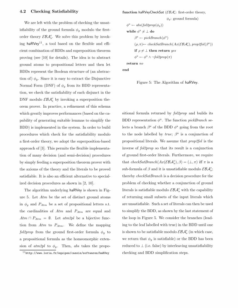
The algorithm underlying haRVey is shown in Fig-

ure 5. Let Atm be the set of distinct ground atoms

in φg and PAtm be a set of propositional letters s.t.

the cardinalities of Atm and PAtm are equal and

Atm ∩ PAtm = ∅. Let atm2pl be a bijective func-

tion from Atm to PAtm. We define the mapping

fol2prop from the ground first-order formula φg to

a propositional formula as the homeomorphic exten-

sion of atm2pl to φg . Then, abs takes the propo-

11http://www.loria.fr/equipes/cassis/softwares/haRVey

function haRVeyCheckSat (EBAes: first-order theory,

φg: ground formula)

φa ← abs(fol2prop(φg))

while φa 6= ⊥ do

βa ← pickBranch(φa)

(ρ, π)← checkSatBranch (Ax(EBAes), prop2fol(β

a))

if ρ 6= ⊥ then return yes

φa ← φa ∧ ¬fol2prop(π)

return no

end

Figure 5: The Algorithm of haRVey.

sitional formula returned by fol2prop and builds its

BDD representation φa. The function pickBranch se-

lects a branch βa of the BDD φa going from the root

to the node labelled by true; βa is a conjunction of

propositional literals. We assume that prop2fol is the

inverse of fol2prop so that its result is a conjunction

of ground first-order literals. Furthermore, we require

that checkSatBranch(Ax(EBAes), β) = (⊥, π) iff π is a

sub-formula of β and it is unsatisfiable modulo EBAes;

thereby checkSatBranch is a decision procedure for the

problem of checking whether a conjunction of ground

literals is satisfiable modulo EBAes with the capability

of returning small subsets of the input literals which

are unsatisfiable. Such a set of literals can then be used

to simplify the BDD, as shown by the last statement of

the loop in Figure 5. We consider the branches (lead-

ing to the leaf labelled with true) in the BDD until one

is shown to be satisfiable modulo EBAes (in which case,

we return that φg is satisfiable) or the BDD has been

reduced to ⊥ (i.e. false) by interleaving unsatisfiability

checking and BDD simplification steps.

4.3 Providing the User with Counter-

Examples

If a branch β has been found satisfiable by haR-

Vey, then we can use it as the starting point to build

a model for the formula φg under consideration, i.e.

a counter-example for the formula to be proved valid

(which is the negation of φg). Notice that this is an ad-

vantage w.r.t. building a model for the whole formula

φg since the branch is usually much smaller.

In preliminary investigations, we have tried to build

a (finite) model of β by using state-of-the-art model

finders (such as MACE12 and SEM13) without suc-

cess. As a matter of fact, the theory EBAes generates

a search space which is too large to be treated in a rea-

sonable amount of time. In order to overcome these

difficulties, we have investigated the possibility to use

the CLPS tool [5], a constraint solver for the theory

of Hereditarily Finite Sets with Atoms which includes

SSET . This tool has already been successfully used on

industrial verification problems. Since the input lan-

guage of CLPS is based on set theoretic constructs, we

need to translate the branch β back to a conjunction η

of literals in SSET . Once the universal set of the AM

(cf. the set PID in Figure 1) is manually instantiated to

a certain finite set, CLPS can find a solution (if any)

to η which (possibly) constitutes a transition of (an

instance of) the AM leading to a state which violates

the invariant. However, notice that we are not guar-

anteed that such a state is reachable by executing the

AM starting in the initial state (specified by the clause

INITIALISATION in Figure 1). To establish whether

the state is reachable or not, two solutions are possi-

ble. First, one can use an animation tool (e.g. the one

12http://www-unix.mcs.anl.gov/AR/mace2/13http://www.cs.uiowa.edu/~hzhang/sem.html

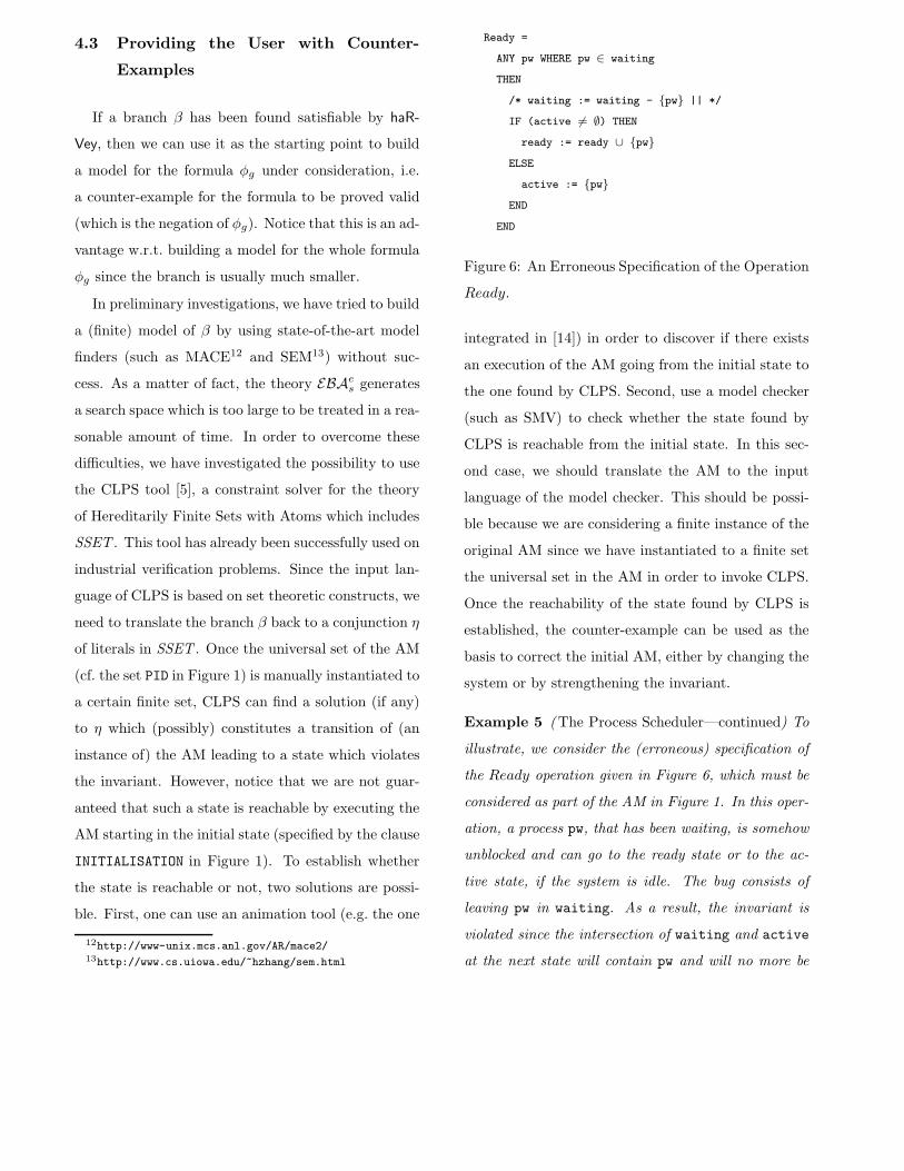
Ready =

ANY pw WHERE pw ∈ waiting

THEN

/* waiting := waiting - {pw} || */

IF (active 6= ∅) THEN

ready := ready ∪ {pw}

ELSE

active := {pw}

END

END

Figure 6: An Erroneous Specification of the Operation

Ready.

integrated in [14]) in order to discover if there exists

an execution of the AM going from the initial state to

the one found by CLPS. Second, use a model checker

(such as SMV) to check whether the state found by

CLPS is reachable from the initial state. In this sec-

ond case, we should translate the AM to the input

language of the model checker. This should be possi-

ble because we are considering a finite instance of the

original AM since we have instantiated to a finite set

the universal set in the AM in order to invoke CLPS.

Once the reachability of the state found by CLPS is

established, the counter-example can be used as the

basis to correct the initial AM, either by changing the

system or by strengthening the invariant.

Example 5 (The Process Scheduler—continued) To

illustrate, we consider the (erroneous) specification of

the Ready operation given in Figure 6, which must be

considered as part of the AM in Figure 1. In this oper-

ation, a process pw, that has been waiting, is somehow

unblocked and can go to the ready state or to the ac-

tive state, if the system is idle. The bug consists of

leaving pw in waiting. As a result, the invariant is

violated since the intersection of waiting and active

at the next state will contain pw and will no more be

empty. (Notice that to correct the problem it is suf-

ficient to uncomment the line delimited by /* and */

in Figure 6.) We want to detect the anomalous situa-

tion by using the approach described above. First, we

generate the verification condition (along the lines of

Section 2). Then, we translate and manipulate the re-

sulting formula so that haRVey can process it (cf. Sec-

tions 3 and 4). The system finds that the proof obliga-

tion is not valid and returns the following set of liter-

als (intended conjunctively): {q0, q1, q2, q3, active =

mty, waiting′ = waiting, ready′ = ready, active′ =

i25, rd(waiting, pw) = tt, i17 = mty, i14 = mty, i11 =

mty, i35 6= mty}.14 As the reader can see, it is quite

difficult to understand the problem in the specification

by looking at this set of literals, even for this simple

example. As a matter of fact, it is rather obscure to

see the meaning of the propositional letters q0, ..., q3

and of the constants i25, ..., i35 which have been intro-

duced to eliminate set-theoretic constructs and quan-

tifiers as specified in Sections 3 and 4.1. However,

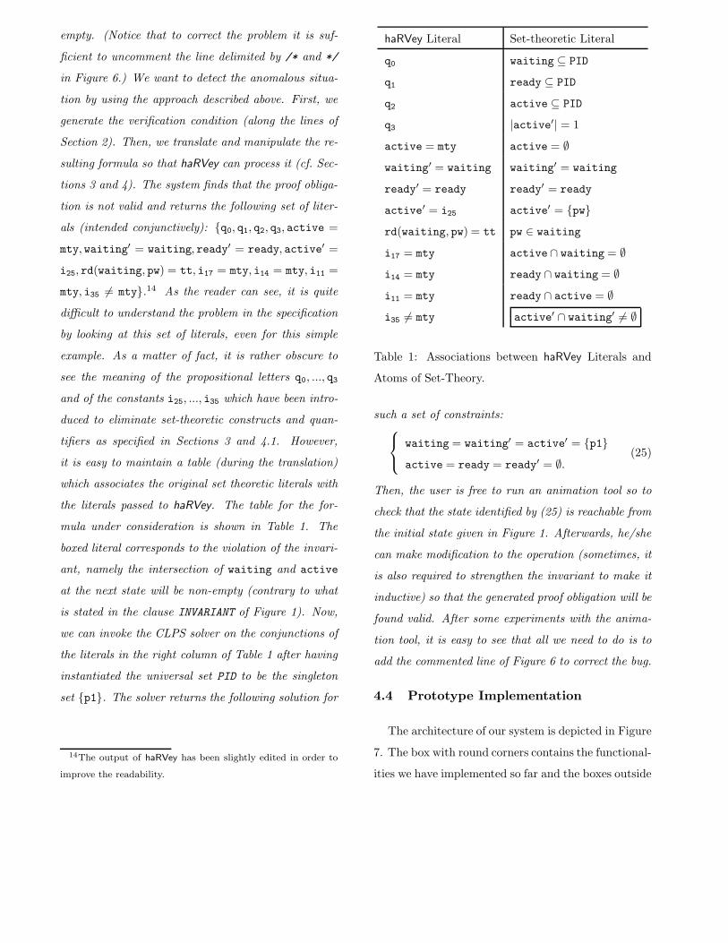
it is easy to maintain a table (during the translation)

which associates the original set theoretic literals with

the literals passed to haRVey. The table for the for-

mula under consideration is shown in Table 1. The

boxed literal corresponds to the violation of the invari-

ant, namely the intersection of waiting and active

at the next state will be non-empty (contrary to what

is stated in the clause INVARIANT of Figure 1). Now,

we can invoke the CLPS solver on the conjunctions of

the literals in the right column of Table 1 after having

instantiated the universal set PID to be the singleton

set {p1}. The solver returns the following solution for

14The output of haRVey has been slightly edited in order to

improve the readability.

haRVey Literal Set-theoretic Literal

q0 waiting ⊆ PID

q1 ready ⊆ PID

q2 active ⊆ PID

q3 |active′| = 1

active = mty active = ∅waiting′ = waiting waiting′ = waiting

ready′ = ready ready′ = ready

active′ = i25 active′ = {pw}rd(waiting, pw) = tt pw ∈ waiting

i17 = mty active∩ waiting = ∅i14 = mty ready ∩ waiting = ∅i11 = mty ready ∩ active = ∅i35 6= mty active′ ∩ waiting′ 6= ∅

Table 1: Associations between haRVey Literals and

Atoms of Set-Theory.

such a set of constraints:

waiting = waiting′ = active′ = {p1}active = ready = ready′ = ∅.

(25)

Then, the user is free to run an animation tool so to

check that the state identified by (25) is reachable from

the initial state given in Figure 1. Afterwards, he/she

can make modification to the operation (sometimes, it

is also required to strengthen the invariant to make it

inductive) so that the generated proof obligation will be

found valid. After some experiments with the anima-

tion tool, it is easy to see that all we need to do is to

add the commented line of Figure 6 to correct the bug.

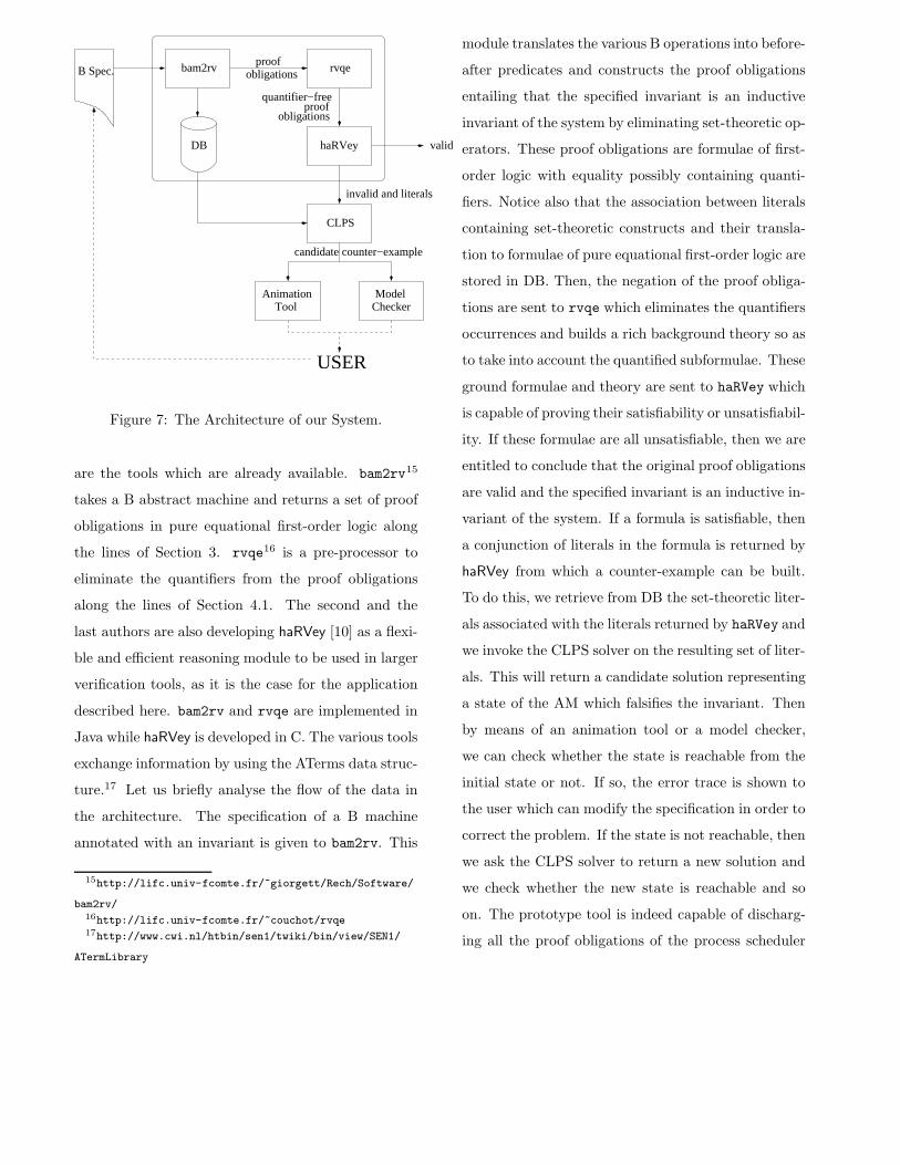
4.4 Prototype Implementation

The architecture of our system is depicted in Figure

7. The box with round corners contains the functional-

ities we have implemented so far and the boxes outside

B Spec. bam2rv rvqe

haRVeyDB

CLPS

AnimationTool Checker

Model

obligationsproof

proofquantifier−free

obligations

valid

invalid and literals

candidate counter−example

USER

Figure 7: The Architecture of our System.

are the tools which are already available. bam2rv15

takes a B abstract machine and returns a set of proof

obligations in pure equational first-order logic along

the lines of Section 3. rvqe16 is a pre-processor to

eliminate the quantifiers from the proof obligations

along the lines of Section 4.1. The second and the

last authors are also developing haRVey [10] as a flexi-

ble and efficient reasoning module to be used in larger

verification tools, as it is the case for the application

described here. bam2rv and rvqe are implemented in

Java while haRVey is developed in C. The various tools

exchange information by using the ATerms data struc-

ture.17 Let us briefly analyse the flow of the data in

the architecture. The specification of a B machine

annotated with an invariant is given to bam2rv. This

15http://lifc.univ-fcomte.fr/~giorgett/Rech/Software/

bam2rv/16http://lifc.univ-fcomte.fr/~couchot/rvqe17http://www.cwi.nl/htbin/sen1/twiki/bin/view/SEN1/

ATermLibrary

module translates the various B operations into before-

after predicates and constructs the proof obligations

entailing that the specified invariant is an inductive

invariant of the system by eliminating set-theoretic op-

erators. These proof obligations are formulae of first-

order logic with equality possibly containing quanti-

fiers. Notice also that the association between literals

containing set-theoretic constructs and their transla-

tion to formulae of pure equational first-order logic are

stored in DB. Then, the negation of the proof obliga-

tions are sent to rvqe which eliminates the quantifiers

occurrences and builds a rich background theory so as

to take into account the quantified subformulae. These

ground formulae and theory are sent to haRVey which

is capable of proving their satisfiability or unsatisfiabil-

ity. If these formulae are all unsatisfiable, then we are

entitled to conclude that the original proof obligations

are valid and the specified invariant is an inductive in-

variant of the system. If a formula is satisfiable, then

a conjunction of literals in the formula is returned by

haRVey from which a counter-example can be built.

To do this, we retrieve from DB the set-theoretic liter-

als associated with the literals returned by haRVey and

we invoke the CLPS solver on the resulting set of liter-

als. This will return a candidate solution representing

a state of the AM which falsifies the invariant. Then

by means of an animation tool or a model checker,

we can check whether the state is reachable from the

initial state or not. If so, the error trace is shown to

the user which can modify the specification in order to

correct the problem. If the state is not reachable, then

we ask the CLPS solver to return a new solution and

we check whether the new state is reachable and so

on. The prototype tool is indeed capable of discharg-

ing all the proof obligations of the process scheduler

discussed here and to detect the invalidity of those

generated from some buggy versions.

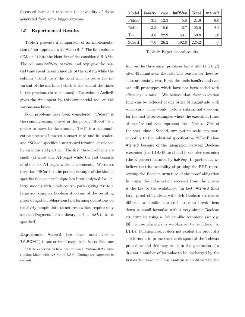
4.5 Experimental Results

Table 2 presents a comparison of an implementa-

tion of our approach with AtelierB.18 The first column

(“Model”) lists the identifier of the considered B AMs.

The columns haRVey, bam2rv, and rvqe give the par-

tial time spent in each module of the system while the

column “Total” lists the total time to prove the in-

variant of the machine (which is the sum of the times

in the previous three columns). The column AtelierB

gives the time spent by this commercial tool on the

various machines.

Four problems have been considered: “Pidset” is

the running example used in this paper, “Robot” is a

device to move blocks around, “T=1” is a communi-

cation protocol between a smart card and its reader,

and “SCard” specifies a smart card terminal developed

by an industrial partner. The first three problems are

small (at most one A4-page) while the last consists

of about six A4-pages without comments. We stress

here that “SCard” is the perfect example of the kind of

specifications our technique has been designed for, i.e.

large models with a rich control path (giving rise to a

large and complex Boolean structure of the resulting

proof obligation obligations) performing operations on

relatively simple data structures (which require only

selected fragments of set theory, such as SSET , to be

specified).

Experience. AtelierB (we have used version

3.6 BOM.1) is one order of magnitude faster than our

18All the experiments have been run on a Pentium II 250 Mhz

running Linux with 128 Mb of RAM. Timings are expressed in

seconds.

Model bam2rv rvqe haRVey Total AtelierB

Pidset 3.5 12.3 5.8 21.6 6.0

Robot 3.3 15.0 6.7 25.0 2.1

T=1 3.6 22.9 43.1 69.8 1.0

SCard 7.0 26.2 192.0 225.2√

Table 2: Experimental results.

tool on the three small problems but it aborts (cf.√

)

after 45 minutes on the last. The reasons for these re-

sults are mainly two. First, the tools bam2rv and rvqe

are still prototypes which have not been coded with

efficiency in mind. We believe that their execution

time can be reduced of one order of magnitude with

some care. This would yield a substantial speed-up

for the first three examples where the execution times

of bam2rv and rvqe represent from 50% to 70% of

the total time. Second, our system scales up more

smoothly to the industrial specification “SCard” than

AtelierB because of the integration between Boolean

reasoning (the BDD library) and first-order reasoning

(the E prover) featured by haRVey. In particular, we

believe that its capability of pruning the BDD repre-

senting the Boolean structure of the proof obligation

by using the information received from the prover

is the key to the scalability. In fact, AtelierB finds

large proof obligations with rich Boolean structures

difficult to handle because it tries to break them

down to small formulae with a very simple Boolean

structure by using a Tableau-like technique (see e.g.

[8]), whose efficiency is well-known to be inferior to

BDDs. Furthermore, it does not exploit the proof of a

sub-formula to prune the search space of the Tableau

procedure and this may result in the generation of a

dramatic number of formulae to be discharged by the

first-order reasoner. This analysis is confirmed by the

fact that for “SCard”, AtelierB generates more than

10, 000 formulae (its maximal bound) after about 45

minutes.

We have also built a prototype tool which encodes

the proof obligations in the logic of WS1S19 so that the

system Mona [13] can be invoked. On “SCard”, Mona

runs out of memory after two hours of computation,

having built more than 140 automata in memory.

We believe that these preliminary results confirm

the viability of our approach.

5 Conclusion and Future Work

We have presented a technique to prove invariants

of model-based specifications in a fragment of set the-

ory. Proof obligations containing set theory constructs

are translated to first-order logic with equality aug-

mented with (an extension of) the theory of arrays

with extensionality. A theorem proving procedure au-

tomating the verification of the proof obligations ob-

tained by the translation has also been described. The

technique has been implemented and experimental re-

sults confirm the viability of our approach.

The lines of future research are essentially fourfold.

First, we envisage extending the decidability result for

Aes in [3] to the theory BAe

s considered in this pa-

per. Second, we plan to handle a larger number of

constructs: on the one hand we will integrate oper-

ators as Cartesian product and relations which are

commonly used in state-based specifications and, on

the other hand, we will add some B syntactic sugar.

Third, we want to integrate the CLPS solver in our

tool so that meaningful counter-examples can be au-

tomatically built from failed proof attempts. Finally,

19This is possible as observed in Section 3.5.

we plan to apply our technique to a larger number of

case studies.

Acknowledgement

We thank Frederic Dadeau for his implementation

of bam2rv and many useful discussions on the work

reported in the paper. We would also like to thank

Dominique Cansell and Stephan Merz for useful com-

ments on a preliminary version of this paper.

References

[1] J.-R. Abrial. The B-Book: Assigning Programs

to Meanings. Cambridge University Press, 1996.

[2] A. Armando, M.P. Bonacina, S. Ranise, M. Rusi-

nowitch, and A. K. Sehgal. High-Performance De-

duction for Verification: A Case Study in the The-

ory of Arrays. In Proc. of VERIFY’02 (FLoC’02

Affiliated Wokshop), 2002.

[3] A. Armando, S. Ranise, and M. Rusinowitch. A

Rewriting Approach to Satisfiability Procedures.

Info. and Comp., 183(2):140–164, June 2003.

[4] J.-P. Bodeveix and M. Filali. Type Synthesis in

B and the Translation of B to PVS. In Proc. of

ZB 2002, volume 2272 of LNCS, pages 350–369.

Springer Verlag, 2002.

[5] F. Bouquet, B. Legeard, and F. Peureux. CLPS-B

- A Constraint Solver for B. In International Con-

ference on Tools and Algorithms for Construction

and Analysis of Systems, TACAS2002, volume

2280 of LNCS, pages 188–204. Springer Verlag,

2002.

[6] J. R. Buchi. Weak second order arithmetic and

finite automata. Zeitschr. f. math. Logik und

Grundlagen d. Math., 6:66–92, 1960.

[7] C.-L. Chang and R. C.-T. Lee. Symbolic Logic and

Mechanical Theorem Proving. Academic Press,

1973.

[8] M. D’Agostino, D. M. Gabbay, R. Hhnle, and

J. Posegga, editors. Handbook of Tableau Meth-

ods. Kluwer Ac. Publ., Dordrecht, 1999.

[9] J. Dawes. The VDM-SL Reference Guide. Pit-

man, 1991.

[10] D. Deharbe and S. Ranise. Light-weight theorem

proving for debugging and verifying units of code.

In International Conference on Software Engi-

neering and Formal Methods (SEFM03). IEEE

Computer Society Press, 2003.

[11] J. Dick and A. Faivre. Automating the Genera-

tion and Sequencing of Test Cases from Model-

Based Specifications. In Proc. of FME’93, vol-

ume 670 of LNCS, pages 268–284. Springer Ver-

lag, 1993.

[12] H. B. Enderton. A Mathematical Introduction to

Logic. Ac. Press, Inc., 1972.

[13] J. G. Henriksen, J. L. Jensen, M. E. Jørgensen,

N. Klarlund, R. Paige, T. Rauhe, and A. Sand-

holm. Mona: Monadic second-order logic in prac-

tice. In Proc. of Tools and Algorithms for the

Construction and Analysis of Systems, volume

1019 of LNCS, pages 89–110. Springer Verlag,

1996.

[14] M. Leuschel and M. Butler. The ProB Animator

and Model Checker for B. In Proc. 12th Interna-

tional FME Symposium 2003 (FM2003), 2003.

[15] L. Mikhailov and M. Butler. An Approach to

Combining B and Alloy. In Proc. of ZB 2002,

volume 2272 of LNCS, pages 140–161. Springer

Verlag, 2002.

[16] R. Nieuwenhuis and A. Rubio. Paramodulation-

based theorem proving. In A. Robinson and

A. Voronkov, editors, Hand. of Automated Rea-

soning. 2001.

[17] N. Shankar. Little Engines of Proof. In For-

mal Methods Europe (FME’02), volume 2391 of

LNCS, pages 1–20. Springer-Verlag, 2002.

[18] M. Spivey. The Z Notation: A Reference Manual.

Prentice Hall, 2nd edition, 1992.

[19] C. Weidenbach and A. Nonnengart. Handbook of

automated reasoning, vol.1, 2001. A. Robinson

and A. Voronkov editors. Elsevier Science.