Performance Debugging Toolbox for Binaries: Sensitivity ...
183
HAL Id: tel-02908498 https://tel.archives-ouvertes.fr/tel-02908498 Submitted on 29 Jul 2020 HAL is a multi-disciplinary open access archive for the deposit and dissemination of sci- entific research documents, whether they are pub- lished or not. The documents may come from teaching and research institutions in France or abroad, or from public or private research centers. L’archive ouverte pluridisciplinaire HAL, est destinée au dépôt et à la diffusion de documents scientifiques de niveau recherche, publiés ou non, émanant des établissements d’enseignement et de recherche français ou étrangers, des laboratoires publics ou privés. Performance Debugging Toolbox for Binaries : Sensitivity Analysis and Dependence Profiling Fabian Gruber To cite this version: Fabian Gruber. Performance Debugging Toolbox for Binaries : Sensitivity Analysis and Depen- dence Profiling. Mathematical Software [cs.MS]. Université Grenoble Alpes, 2019. English. NNT : 2019GREAM071. tel-02908498
-
Upload
khangminh22 -
Category
Documents
-
view
1 -
download
0
Transcript of Performance Debugging Toolbox for Binaries: Sensitivity ...

HAL Id: tel-02908498https://tel.archives-ouvertes.fr/tel-02908498
Submitted on 29 Jul 2020
HAL is a multi-disciplinary open accessarchive for the deposit and dissemination of sci-entific research documents, whether they are pub-lished or not. The documents may come fromteaching and research institutions in France orabroad, or from public or private research centers.
L’archive ouverte pluridisciplinaire HAL, estdestinée au dépôt et à la diffusion de documentsscientifiques de niveau recherche, publiés ou non,émanant des établissements d’enseignement et derecherche français ou étrangers, des laboratoirespublics ou privés.
Performance Debugging Toolbox for Binaries :Sensitivity Analysis and Dependence Profiling
Fabian Gruber
To cite this version:Fabian Gruber. Performance Debugging Toolbox for Binaries : Sensitivity Analysis and Depen-dence Profiling. Mathematical Software [cs.MS]. Université Grenoble Alpes, 2019. English. �NNT :2019GREAM071�. �tel-02908498�

THÈSEPour obtenir le grade de
DOCTEUR DE L’UNIVERSITÉ GRENOBLE ALPESSpécialité : InformatiqueArrêté ministériel : 25 mai 2016
Présentée par
Fabian GRUBER
Thèse dirigée par Fabrice RASTELLO
préparée au sein du Laboratoire d'Informatique de Grenobledans l'École Doctorale Mathématiques, Sciences et technologies de l'information, Informatique
Débogage de performance pour code binaire:Analyse de sensitivité et profilage de dépendances
Performance Debugging Toolbox for Binaries:Sensitivity Analysis and Dependence Profiling
Thèse soutenue publiquement le 17 décembre 2019,devant le jury composé de :
Monsieur FABRICE RASTELLODIRECTEUR DE RECHERCHE, INRIA CENTRE DE GRENOBLE RHÔNE-ALPES, Directeur de thèseMonsieur BARTON MILLERPROFESSEUR, UNIVERSITY OF WISCONSIN-MADISON – USA, RapporteurMonsieur DENIS BARTHOUPROFESSEUR, BORDEAUX INP, RapporteurMonsieur FRANZ FRANCHETTIPROFESSEUR, CARNEGIE MELLON UNIVERSITY – USA, ExaminateurMonsieur FREDERIC PETROTPROFESSEUR, GRENOBLE INP, PrésidentMonsieur SVILEN KANEVDOCTEUR-INGENIEUR, GOOGLE – USA, Examinateur


iii
Résumé
Le débogage, tel qu’il est généralement défini, consiste à trouver et à supprimer les problèmesempêchant un logiciel de fonctionner correctement. Quand on parle de bogues et de débogage,on fait donc habituellement référence à des bogues fonctionnels et au débogage fonctionnel. Dansle contexte de cette thèse, cependant, nous parlerons des bogues de performance et de débogage deperformance. Nous ne cherchons donc pas les problèmes engendrant de mauvais comportementsdu programme, mais les problèmes qui le rendent inefficace, trop lent, ou qui induisent une tropgrande utilisation de ressources. À cette fin, nous avons développé des outils qui analysent etmodélisent la performance pour aider les programmeurs à améliorer leur code de ce point devue là. Nous proposons les deux techniques de débogage de performance suivantes: analyse desgoulets d’étranglement basée sur la sensibilité et Suggestions d’optimisation polyédrique baséessur les dépendances de données.
Analyse des goulets d’étranglement basée sur la sensibilité Il peut être étonnammentdifficile de répondre à une question apparemment anodine sur la performance d’un programme,comme par exemple celle de savoir s’il est limité par la mémoire ou par le CPU. En effet, le CPUet la mémoire ne sont pas deux ressources complètement indépendantes, mais sont composésde multiples sous-systèmes complexes et interdépendants. Ici, un blocage d’une ressource peutà la fois masquer ou aggraver des problèmes avec une autre ressource. Nous présentons uneanalyse des goulets d’étranglement basée sur la sensibilité qui utilise un modèle de performancede haut niveau implémenté dans Gus, un simulateur CPU rapide pour identifier les gouletsd’étranglement de performance.
Notre modèle de performance a besoin d’une base de référence pour la performance attenduedes différentes opérations sur un CPU, comme le pic IPC et comment différentes instructionsse partagent les ressources du processeur. Malheureusement, cette information est rarementpubliée par les fournisseurs de matériel, comme Intel ou AMD. Pour construire notre modèle deprocesseur, nous avons développé un système permettant de récupérer les informations requisesen utilisant des micro-benchmarks générés automatiquement.
Suggestions d’optimisation polyédrique basées sur les dépendances de données Nousavons développé Mickey, un profileur dynamique de dépendances de données qui fournit un re-tour d’optimisation de haut niveau sur l’applicabilité et la rentabilité des optimisations manquéespar le compilateur. Mickey exploite le modèle polyédrique, un puissant cadre d’optimisationpour trouver des séquences de transformations de boucle afin d’exposer la localité des donnéeset d’implémenter à la fois le parallélisme gros-grain, c’est-à-dire au niveau thread, et grain-fin, c’est-à-dire au niveau vectoriel. Notre outil utilise une instrumentation binaire dynamiquepour analyser des programmes écrits dans différents langages de programmation ou utilisant desbibliothèques tierces pour lesquelles aucun code source n’est disponible.
En interne Mickey utilise une représentation intermédiaire (RI) polyédrique qui code àla fois l’exécution dynamique des instructions d’un programme ainsi que ses dépendances dedonnées. La RI ne capture pas seulement les dépendances de données à travers plusieurs bouclesmais aussi à travers des appels de procédure, éventuellement récursifs. Nous avons développéun algorithme efficace de compression de traces qui construit cette RI polyédrique à partir del’exécution d’un programme. L’folding algorithm trouve aussi des accès réguliers dans les accèsmémoire pour prédire la possibilité et la rentabilité de la vectorisation. Il passe à l’échelle sur degros programmes grâce à un mécanisme de sur-approximation sûr et sélectif pour les applicationspartiellement irrégulières.

iv

v
Abstract
Debugging, as usually understood, revolves around finding and removing defects in softwarethat prevent it from functioning correctly. That is, when one talks about bugs and debugging oneusually means functional bugs and functional debugging. In the context of this thesis, however,we will talk about performance bugs and performance debugging. Meaning we want to find defectsthat do not cause a program to crash or behave wrongly, but that make it run inefficiently, tooslow, or use too many resources. To that end, we have developed tools that analyse and modelthe performance to help programmers improve their code to get better performance. We proposethe following two performance debugging techniques: sensitivity based bottleneck analysis anddata-dependence profiling driven optimization feedback.
Sensitivity Based Performance Bottleneck Analysis Answering a seemingly trivial ques-tion about a program’s performance, such as whether it is memory-bound or CPU-bound, canbe surprisingly difficult. This is because the CPU and memory are not merely two completelyindependent resources, but are composed of multiple complex interdependent subsystems. Herea stall of one resource can both mask or aggravate problems with another resource. We presenta sensitivity based performance bottleneck analysis that uses high-level performance model im-plemented in Gus, a fast CPU simulator to pinpoint performance bottlenecks.
Our performance model needs a baseline for the expected performance of different operationson a CPU, like the peak IPC and how different instructions compete for processor resources.Unfortunately, this information is seldom published by hardware vendors, such as Intel or AMD.To build our processor model, we have developed a system to reverse-engineer the requiredinformation using automatically generated micro-benchmarks.
Data-Dependence Driven Polyhedral Optimization Feedback We have developedMickey, a dynamic data-dependence profiler that provides high-level optimization feedback onthe applicability and profitability of optimizations missed by the compiler. Mickey leveragesthe polyhedral model, a powerful optimization framework for finding sequences of loop trans-formations to expose data locality and implement both coarse, i.e. thread, and fine-grain, i.e.vector-level, parallelism. Our tool uses dynamic binary instrumentation allowing it to analyzeprogram written in different programming languages or using third-party libraries for which nosource code is available.
Internally Mickey uses a polyhedral intermediate representation (IR) that encodes boththe dynamic execution of a program’s instructions as well as its data dependencies. The IRnot only captures data dependencies across multiple loops but also across, possibly recursive,procedure calls. We have developed an efficient trace compression algorithm, called the foldingalgorithm, that constructs this polyhedral IR from a program’s execution. The folding algorithmalso finds strides in memory accesses to predict the possibility and profitability of vectorization.It can scale to real-life applications thanks to a safe, selective over-approximation mechanismfor partially irregular data dependencies and iteration spaces.

vi

Dedication
This thesis is dedicated to my future wife Kim Hyunyoung, my family, and my friends.Thank you from the bottom of my heart.
vii

viii

Acknowledgements
The work presented in this thesis has been done in collaboration with my advisor FabriceRastello, Louis-Noël Pouchet from the Colorado State University, Christophe Guillon and othersfrom STMicroelectronics, my colleagues Diogo Nunes Sampaio, Manuel Selva, Nicolas Tollenare,Nicolas Derumigny, and many more.I sincerely thank them all for their advice, help, and hard work.Without them my thesis would not have been possible.I also sincerely thank Imma Presseguer for all the administrative work, moral support andadvice.
ix

x

Contents
Résumé iii
Abstract v
Contents xi
1 Introduction 11.1 Performance Debugging . . . . . . . . . . . . . . . . . . . . . . . . . . . . . . . . 31.2 Background . . . . . . . . . . . . . . . . . . . . . . . . . . . . . . . . . . . . . . . 3
1.2.1 Profiling . . . . . . . . . . . . . . . . . . . . . . . . . . . . . . . . . . . . . 31.2.2 Instrumentation and dynamic binary analysis . . . . . . . . . . . . . . . . 51.2.3 The polyhedral model . . . . . . . . . . . . . . . . . . . . . . . . . . . . . 6
1.3 Objectives . . . . . . . . . . . . . . . . . . . . . . . . . . . . . . . . . . . . . . . . 81.3.1 Sensitivity Based Performance Bottleneck Analysis . . . . . . . . . . . . . 81.3.2 Dependence Profiling Driven Polyhedral Optimization Feedback . . . . . 91.3.3 Contributions . . . . . . . . . . . . . . . . . . . . . . . . . . . . . . . . . . 10
1.4 Structure of the Thesis . . . . . . . . . . . . . . . . . . . . . . . . . . . . . . . . . 10
2 Dynamic Binary Instrumentation with QEMU 112.1 QEMU . . . . . . . . . . . . . . . . . . . . . . . . . . . . . . . . . . . . . . . . . . 122.2 The Tiny Code Generator . . . . . . . . . . . . . . . . . . . . . . . . . . . . . . . 132.3 The TCG Plugin Infrastructure . . . . . . . . . . . . . . . . . . . . . . . . . . . . 162.4 Execution Tracing with QEMU . . . . . . . . . . . . . . . . . . . . . . . . . . . . 19
2.4.1 Control-flow tracing . . . . . . . . . . . . . . . . . . . . . . . . . . . . . . 202.4.2 Data Dependence Tracing . . . . . . . . . . . . . . . . . . . . . . . . . . . 272.4.3 Value tracing . . . . . . . . . . . . . . . . . . . . . . . . . . . . . . . . . . 28
2.5 Evaluation of the Overhead of Plugins . . . . . . . . . . . . . . . . . . . . . . . . 282.6 Related Work . . . . . . . . . . . . . . . . . . . . . . . . . . . . . . . . . . . . . . 292.7 Conclusion and Perspectives . . . . . . . . . . . . . . . . . . . . . . . . . . . . . . 34
3 Sensitivity Based Performance Bottleneck Analysis 353.1 Introduction . . . . . . . . . . . . . . . . . . . . . . . . . . . . . . . . . . . . . . . 363.2 Modern CPU Microarchitecture . . . . . . . . . . . . . . . . . . . . . . . . . . . . 38
3.2.1 Concepts of instruction level parallelism . . . . . . . . . . . . . . . . . . . 383.2.2 Implementation of instruction level parallelism . . . . . . . . . . . . . . . 39
3.3 Related Work . . . . . . . . . . . . . . . . . . . . . . . . . . . . . . . . . . . . . . 413.4 Gus . . . . . . . . . . . . . . . . . . . . . . . . . . . . . . . . . . . . . . . . . . . 48
3.4.1 A resource-centric CPU model . . . . . . . . . . . . . . . . . . . . . . . . 493.4.2 An illustrative example . . . . . . . . . . . . . . . . . . . . . . . . . . . . 503.4.3 The simulator algorithm . . . . . . . . . . . . . . . . . . . . . . . . . . . . 54
3.5 Pipedream . . . . . . . . . . . . . . . . . . . . . . . . . . . . . . . . . . . . . . . . 56
xi

xii CONTENTS
3.5.1 The instruction flow problem . . . . . . . . . . . . . . . . . . . . . . . . . 573.5.2 Finding port mappings . . . . . . . . . . . . . . . . . . . . . . . . . . . . . 613.5.3 Converting port mappings to resource models . . . . . . . . . . . . . . . . 653.5.4 Benchmark design . . . . . . . . . . . . . . . . . . . . . . . . . . . . . . . 66
3.6 Experiments . . . . . . . . . . . . . . . . . . . . . . . . . . . . . . . . . . . . . . . 693.6.1 Gus . . . . . . . . . . . . . . . . . . . . . . . . . . . . . . . . . . . . . . . 693.6.2 Pipedream . . . . . . . . . . . . . . . . . . . . . . . . . . . . . . . . . . . 78
3.7 Conclusion and Future Work . . . . . . . . . . . . . . . . . . . . . . . . . . . . . 85
4 Data-Dependence Driven Optimization Feedback 894.1 Introduction . . . . . . . . . . . . . . . . . . . . . . . . . . . . . . . . . . . . . . . 904.2 Illustrative Scenario . . . . . . . . . . . . . . . . . . . . . . . . . . . . . . . . . . 91
4.2.1 Example problem: backprop . . . . . . . . . . . . . . . . . . . . . . . . . . 914.2.2 Solution: Mickey . . . . . . . . . . . . . . . . . . . . . . . . . . . . . . . 93
4.3 Overview of Mickey . . . . . . . . . . . . . . . . . . . . . . . . . . . . . . . . . . 944.4 Interprocedural Program Representation . . . . . . . . . . . . . . . . . . . . . . . 96
4.4.1 Control-flow-graph and loop-nesting-tree . . . . . . . . . . . . . . . . . . . 974.4.2 Call-graph and recursive-component-set . . . . . . . . . . . . . . . . . . . 984.4.3 DDG: Dynamic Dependence Graph . . . . . . . . . . . . . . . . . . . . . . 101
4.5 The Folding Algorithm . . . . . . . . . . . . . . . . . . . . . . . . . . . . . . . . . 1064.5.1 Inputs . . . . . . . . . . . . . . . . . . . . . . . . . . . . . . . . . . . . . . 1064.5.2 Outputs . . . . . . . . . . . . . . . . . . . . . . . . . . . . . . . . . . . . . 1084.5.3 Using the output . . . . . . . . . . . . . . . . . . . . . . . . . . . . . . . . 1094.5.4 Overview . . . . . . . . . . . . . . . . . . . . . . . . . . . . . . . . . . . . 1104.5.5 The algorithm . . . . . . . . . . . . . . . . . . . . . . . . . . . . . . . . . 1114.5.6 Complexity analysis . . . . . . . . . . . . . . . . . . . . . . . . . . . . . . 121
4.6 Polyhedral Feedback . . . . . . . . . . . . . . . . . . . . . . . . . . . . . . . . . . 1224.6.1 Polyhedral compilation of folded-DDGs . . . . . . . . . . . . . . . . . . . 1224.6.2 User feedback . . . . . . . . . . . . . . . . . . . . . . . . . . . . . . . . . . 123
4.7 Experimental Results . . . . . . . . . . . . . . . . . . . . . . . . . . . . . . . . . . 1274.7.1 Case studies . . . . . . . . . . . . . . . . . . . . . . . . . . . . . . . . . . . 1284.7.2 Static polyhedral compilers and Rodinia . . . . . . . . . . . . . . . . . . . 1304.7.3 Optimization feedback on Rodinia . . . . . . . . . . . . . . . . . . . . . . 1314.7.4 Trace compression results . . . . . . . . . . . . . . . . . . . . . . . . . . . 134
4.8 Related Work . . . . . . . . . . . . . . . . . . . . . . . . . . . . . . . . . . . . . . 1344.9 Conclusion and Perspectives . . . . . . . . . . . . . . . . . . . . . . . . . . . . . . 138
5 Conclusion and Future Work 1395.1 Summary . . . . . . . . . . . . . . . . . . . . . . . . . . . . . . . . . . . . . . . . 140
5.1.1 Dynamic Binary Instrumentation with QEMU . . . . . . . . . . . . . . . 1405.1.2 Sensitivity-Based Performance Bottleneck Analysis . . . . . . . . . . . . . 1405.1.3 Data-Dependence Driven Optimization Feedback . . . . . . . . . . . . . . 141
5.2 Perspectives . . . . . . . . . . . . . . . . . . . . . . . . . . . . . . . . . . . . . . . 1425.3 List of Publications . . . . . . . . . . . . . . . . . . . . . . . . . . . . . . . . . . . 143
List of Figures 144
List of Tables 146
List of Algorithms 147

CONTENTS xiii
Bibliography 149
Glossary 167

xiv CONTENTS

Chapter 1Introduction
Contents1.1 Performance Debugging . . . . . . . . . . . . . . . . . . . . . . . . . . . . . . . 31.2 Background . . . . . . . . . . . . . . . . . . . . . . . . . . . . . . . . . . . . . 3
1.2.1 Profiling . . . . . . . . . . . . . . . . . . . . . . . . . . . . . . . . . . . 31.2.2 Instrumentation and dynamic binary analysis . . . . . . . . . . . . . . 51.2.3 The polyhedral model . . . . . . . . . . . . . . . . . . . . . . . . . . . 6
1.3 Objectives . . . . . . . . . . . . . . . . . . . . . . . . . . . . . . . . . . . . . . 81.3.1 Sensitivity Based Performance Bottleneck Analysis . . . . . . . . . . . 81.3.2 Dependence Profiling Driven Polyhedral Optimization Feedback . . . . 91.3.3 Contributions . . . . . . . . . . . . . . . . . . . . . . . . . . . . . . . . 10
1.4 Structure of the Thesis . . . . . . . . . . . . . . . . . . . . . . . . . . . . . . . 10
1
2 CHAPTER 1. INTRODUCTION
It is now nearly fifteen years ago that Herb Sutter wrote his famous article “The Free LunchIs Over” [201]. In this piece, he argued that the classical methods of boosting single-coreperformance, such as raising the CPU clock frequency and straight-line instruction throughput,are no longer feasible. He claims that the single-core performance of modern microprocessorshas completely stagnated and that multi-core architectures and concurrent programming modelsare the only way to increase performance going forward. Only a few years later, Hill et al. [94]analysed the state of microprocessor designs of the time and gave some broad recommendationsthat, at least partially, contradict Sutter’s conclusions. One of their recommendations statesthat “Researchers should seek methods of increasing [single] core performance even at a highcost.”.
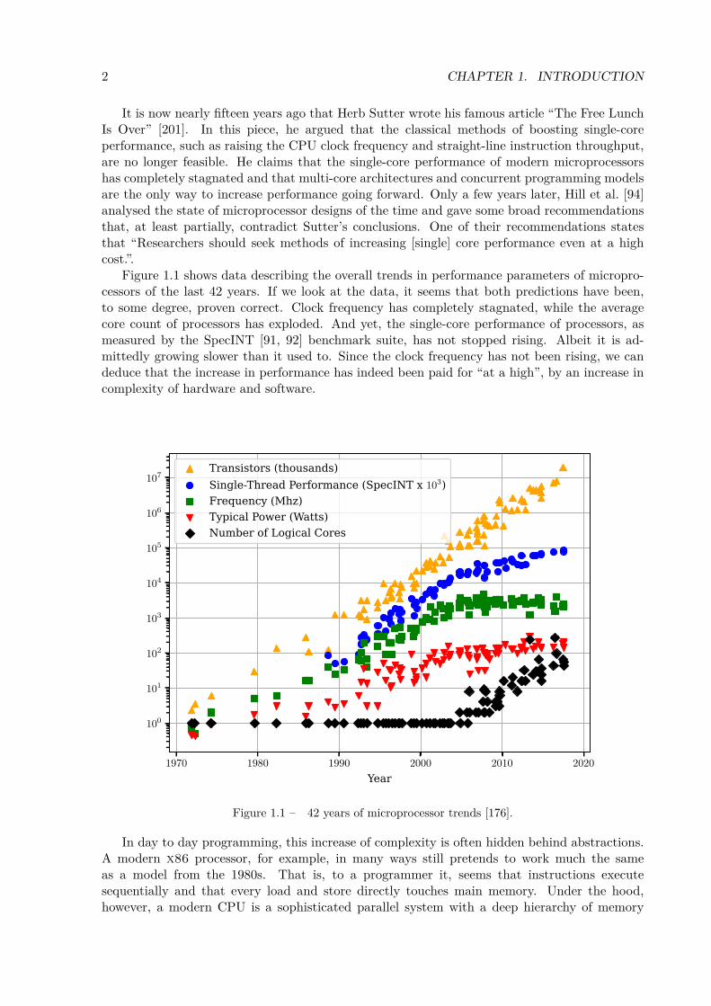
Figure 1.1 shows data describing the overall trends in performance parameters of micropro-cessors of the last 42 years. If we look at the data, it seems that both predictions have been,to some degree, proven correct. Clock frequency has completely stagnated, while the averagecore count of processors has exploded. And yet, the single-core performance of processors, asmeasured by the SpecINT [91, 92] benchmark suite, has not stopped rising. Albeit it is ad-mittedly growing slower than it used to. Since the clock frequency has not been rising, we candeduce that the increase in performance has indeed been paid for “at a high”, by an increase incomplexity of hardware and software.
1970 1980 1990 2000 2010 2020
Year
100
101
102
103
104
105
106
107Transistors (thousands)Single-Thread Performance (SpecINT x 103)Frequency (Mhz)Typical Power (Watts)Number of Logical Cores
Figure 1.1 – 42 years of microprocessor trends [176].
In day to day programming, this increase of complexity is often hidden behind abstractions.A modern x86 processor, for example, in many ways still pretends to work much the sameas a model from the 1980s. That is, to a programmer it, seems that instructions executesequentially and that every load and store directly touches main memory. Under the hood,however, a modern CPU is a sophisticated parallel system with a deep hierarchy of memory

1.1. PERFORMANCE DEBUGGING 3
caches. However, all these abstractions very quickly break down when one wants to study andunderstand the performance of an application. Then it suddenly becomes crucially importantto know which data dependency stopped two instructions from execution in parallel or whichmemory access caused a cache miss. To effectively analyse and debug the performance of aprogram, one has to look under the hood and remove the abstractions. It is the goal of thisthesis to propose tools and techniques for helping programmers better understand the behaviourof their programs and guide them in the process of performance optimization.
1.1 Performance Debugging
Debugging, as usually understood, revolves around finding and removing defects in software thatprevent it from functioning correctly. That is, when one talks about bugs and debugging oneusually means functional bugs and functional debugging. In the context of this thesis, however,we will talk about performance bugs and performance debugging. Meaning we want to find defectsthat do not cause a program to crash or behave wrongly, but that make it run inefficiently, tooslow, or use too many resources.
Even the best programmer has, at some point, written a buggy program. When they observethat something is amiss they will often use functional debugging tools like GDB [74] that helpfind errors in the behaviour of programs. That is, the classical problems for which programmersturn to functional debuggers are:
1. Where is the program misbehaving or crashing?2. Why is the program misbehaving or crashing?
Usually, these tools do not directly try to answer the question how one can prevent a programfrom misbehaving or crashing since this would require changing the semantics of the program.While there are approaches that attempt this from the fields of software verification, like runtimeenforcement [69], they require a specification of the intended semantics of a program and arenot yet commonly used.
Performance debuggers or performance analysis tools, on the other hand, help finding prob-lems in the non-functional aspects of programs. That is, the problems which make a programmerturn to these tools are:
1. Where is the program slow?2. Why is the program slow?3. How can one make the program run faster?
Historically, existing techniques have only measured and predicted the current performancecharacteristics of programs and so, similarly to functional debugging tools, only help answer thefirst two questions. In this thesis, we will develop two approaches that try to extrapolate thepossible performance a system could achieve to help answer the last two questions, i.e., whyprograms are slow and how they can be made more efficient.
1.2 Background
1.2.1 Profiling
The standard approach for identifying performance bugs is profiling. The most straightforwardprofiling technique is to measure the time required to run a piece of code. Tools like gprof [78]help automate this process by automatically inserting code to measure the runtime of individualfunctions via the compiler. Other tools like QPT [122] insert code to count the number of timeevery basic block in a program executes or how many times every edge in the control-flow-graph is taken. These approaches can help detect hot program regions, i.e., where a program is

4 CHAPTER 1. INTRODUCTION
spending most of its time. However, knowing only where the hot regions of a program are is alltoo often not enough to fix performance bugs.
To help pinpoint the causes of performance problems modern processors offer hardware per-formance counters 1, also called hardware counters, or performance counters [44, 151]. Hardwarecounters allow measuring many different performance-related events, such as the number of in-structions executed or the number of cache hits and misses at different cache levels. At themost basic level, performance counters work the same as time measurements. To measure, forexample, the number of L2 cache misses that occur in a given function it suffices to insert codeto read the current value of the corresponding counter at the beginning and the end of thefunction and subtract the two values.
Many processors also support sampling modes which make it possible to use hardware coun-ters without having to modify an application to explicitly read counters. Different vendors andprocessor generations implement a wide variety of different sampling models such as, for exam-ple, event-based sampling, time sampling, and instruction-based sampling. The details of howthese different sampling techniques work, how they can be used, and how precise they differquite a lot. However, the overall idea is that at regular, user-configured intervals the processorhalts normal execution and stores the current values of the hardware performance counters, usu-ally by writing some data to a preconfigured memory location or by raising a special interrupt.Sampling-based profilers then use statistical methods to extrapolate the behaviour of instruc-tions for which they have no samples. Directly using hardware performance counters is quitecomplicated and so over time a plethora of libraries and tools, such as PAPI [65], LIKWID [172],HPCToolkit [4], Linux perf [144], Intel VTune [169], have been developed for this purpose.
Despite their utility hardware performance counters suffer from some severe limitations.While configuring the CPU to count performance events has no, or barely any, overhead, thereading of counters, either directly or through sampling, is not free. Directly reading coun-ters uses at least some CPU resources such as registers and profiling requires either a costlyCPU interrupt or some writes to memory. Consequently using hardware counters can cause anobserver effect where the act of measuring the performance of an application changes its perfor-mance. This can lead to so-called performance heisenbugs, named after Heisenberg’s uncertaintyprinciple. It also makes fine-grain profiling using performance counters difficult.
Linux perf, a widely used sampling-based profiling tool, for example, by default limits themaximum sampling rate. This is to prevent programs from accidentally spending more time read-ing performance counters and writing to internal buffers than actually executing real code [88]On an Intel i5-4590 CPU running at 3.3 GHz the limit is 50k samples per second, which meansone can at best obtain one sample every 66k instructions.
Another problem with performance counters is that one is limited to measuring a fixed set ofmetrics. With this approach, it is impossible to profile for an event for which the hardware offersno counter. Furthermore, even on the most recent processors, one can not enable all availableperformance event counters at the same time, but usually only a small handful, around four toten.
An alternative to using hardware performance counters is to use a simulator such as gem5 [23].A cycle-accurate simulator makes it possible to produce a detailed trace of performance-relatedevents without during execution without perturbing the behaviour of the original program. Sincesimulators are software, it is also possible to add new performance counters if necessary.
However, the power and flexibility of simulators also come at a cost. Developing a cycle-levelsimulator is extremely time consuming and requires a lot of expertise. A detailed simulation isalso quite costly in terms of computation and runs considerably slower than native execution.For example, gem5 at its highest level of precision requires, on average, one year to run a single
1The term “counter” can be misleading since modern processors do much more than just counting events.

1.2. BACKGROUND 5
SPEC2006 benchmark [180]. A common approach to speed up simulations is to only simulateparts of a program [188, 224] or to only simulate some aspect of the processor [36, 110, 152].
Simulators based on abstract high-level CPU core models, while not as accurate as a realcycle-level simulator, have been shown to provide reasonable accurate execution time predictionswhile running orders of magnitude faster than cycle-level simulation systems [68, 76, 202, 37].
At the end of the day, the data gathered using profiling, either using hardware countersor simulation, is still very low-level, recording information at the level of individual machineinstructions. Tools like HPCToolkit [4], Intel VTune [169], and Linux perf [144] can map theseresults back to the source code of a program using debug information, making it possible to viewaggregate results per loop or function. However, these tools still do not directly explain why agiven piece of code has a performance problem, such as too many cache misses or stalled CPUcycles, or how to fix the problem. Finding and fixing the root causes of a performance problemoften still require substantial expertise.
Feedback-Directed Optimization (FDO) takes one step towards the direction of using pro-filing information to improve performance [192, 11, 12]. FDO based systems collect runtimeinformation using profiling and use it to guide optimization heuristics in compilers. Tools like,Intel Advisor [52] and AutoSCOPE [195], on the other hand, try to give human-readable opti-mization advice. They are, however, not able to automatically apply code transformations, oreven necessarily prove that a transformation is valid. Instead, they propose optimizations suchas parallelization or loop fusion, leaving the task of implementing this transformation to theprogrammer.
At this point, we have only given a brief overview of basic profiling techniques. Chapters 3and 4 will present a number of more involved approaches using richer, but expensive to collect,performance events.
1.2.2 Instrumentation and dynamic binary analysis
Since profilers analyse events that occur during the execution of a program, they need somefacility to trace these events. Sampling of hardware performance counters is an excellent lowoverhead method for collecting performance-related events, but it suffers from a number oflimitations, as described in the previous section.
An alternative technique used by a large number of dynamic analysis tools, including thosepresented in this thesis, is instrumentation. Instrumentation, is a very versatile technique thatallows capturing arbitrary program behaviour. Using instrumentation a profiler can implementany new performance counter it may require in software. Besides profiling, instrumentation isused in numerous other dynamic analyses such as dynamic control flow integrity [1] and memorycorruption checking [185].
There are some new hardware-assisted program tracing technologies, such as Intel PT [51],on the horizon that may replace instrumentation for some profiling use cases. However, for themoment the available hardware is still somewhat unreliable and can lose events due to internalbuffer overflows [75, 101].
Compiler based instrumentation, used by highly successful dynamic analysis tools suchgprof [78] and the LLVM Address Sanitizer [185], works directly in the compiler at the levelof its intermediate representation (IR). Instrumenting programs during the compilation processhas several advantages. In terms of productivity, the whole compiler infrastructure makes thetask of implementing some instrumentation for profiling easy. Instrumentation can easily beperformed at any level of the intermediate representation, allowing the profiling of high-leveland low-level properties. It can also take advantage of all its knowledge of the program semanticsand information provided by the diverse static analysis present in an optimizing compiler. Inparticular, any property that can be statically proven or is not data-dependent, does not have

6 CHAPTER 1. INTRODUCTION
to be profiled.Binary instrumentation [196, 123, 134, 155, 134, 29, 145, 146], on the other hand, works
directly at the level of machine code. Analysing and manipulating binaries is difficult andtedious, since, all too often, one has to re-discover the obvious. Because machine code containsmuch less structure than source code even relatively simple analyses needed for instrumentation,such as reconstructing the control-flow graph, become non-trivial or undecidable [145, 170].However, working at the level of machine code has the important advantage of portability. Thatis, tools that directly handle machine code are not restricted to working with a given compiler, orprogramming language. It also makes it possible to compare the binaries produced by differentcompilers. If, for example, icc turns out to generate the best performing code for an Intelplatform, it is clearly interesting to be able to analyse this binary and not be limited to theoutput of GCC [80] or Clang [164]. Binary instrumentation even makes it possible to analyseprograms for which no source code is available or which integrate closed source third-partylibraries.
Another approach that can be used to implement static binary instrumentation is decom-pilation. SecondWrite [8] and DisIRer [104], for example, are two tools that convert machinecode to LLVM IR and GCC IR respectively. These compiler IRs are semantically much richerthan raw machine code, and there are a variety of existing tools that can be used to analyseand transform them. The advantage of this approach is that it has the portability of a binaryanalysis tool combined with ease of use of compiler-based instrumentation. However, it is onlyapplicable to programs that can be statically decompiled.
There are also dynamic binary analysis frameworks that decompile machine code to compilerIR at runtime [64]. However, while this makes it possible to apply the powerful analyses availablein a static compiler to arbitrary binaries, it also suffers from some drawbacks. The main problemis that static compilers can afford to invest much more time in analysing and optimizing programsthan dynamic compilers. Due to this, authors of static compiler IRs and analyses often prioritizeexpressiveness and maintainability over performance. A number of failed attempts to re-usestatic compiler back-ends in a JIT have shown that this can lead to a prohibitive overhead atruntime [49, 50].
Dynamic binary instrumentation and the applications we have used it for will be describedin detail in Chapter 2.
1.2.3 The polyhedral model
The most effective program optimizations for improving performance or energy consumptionare typically based on the rescheduling of instructions to expose data locality, parallelism orboth. The two main challenges for these kinds of optimizations are what transformations maybe applied without breaking the program semantics and where in the program the optimizationsshould be applied to maximize the impact on the overall program performance. The polyhedralmodel [71], a mathematical model that allows reasoning about programs at the levels of loops, isone of the most powerful theoretical frameworks for finding and for applying such reschedulingoptimizations.
The polyhedral model is usually applied in the context of static compilers [160, 211, 81, 162,25, 218]. Here it is used to find sequences of loop transformations, including tiling, permutation,fusion, fission, and skewing, that aim to improve the temporal and spatial locality of data accessesand uncover both coarse (i.e., thread) and fine-grain (i.e., SIMD) parallelism. To determine thevalidity and profitability of these transformations, however, the polyhedral model needs preciseinformation about data and control-flow dependencies. That is, it needs a precise model of thestructure of loops and of the dependencies between statements.
The power of the polyhedral model comes, in part, from the fact that it does not try to model
1.2. BACKGROUND 7
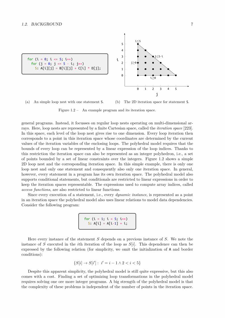
for (i = 0; i <= 5; i++)
for (j = 0; j <= 5 - i; j++)
S: A[i][j] = B[i][j] + C[i] * D[j];
(a) An simple loop nest with one statement S.
0 1 2 3 4 5
0
1
2
3
4
5
j≥0
j≤5-i
i≥0
i≤5
j
i
(b) The 2D iteration space for statement S.
Figure 1.2 – An example program and its iteration space.
general programs. Instead, it focusses on regular loop nests operating on multi-dimensional ar-rays. Here, loop nests are represented by a finite Cartesian space, called the iteration space [223].In this space, each level of the loop nest gives rise to one dimension. Every loop iteration thencorresponds to a point in this iteration space whose coordinates are determined by the currentvalues of the iteration variables of the enclosing loops. The polyhedral model requires that thebounds of every loop can be represented by a linear expression of the loop indices. Thanks tothis restriction the iteration space can also be represented as an integer polyhedron, i.e., a setof points bounded by a set of linear constraints over the integers. Figure 1.2 shows a simple2D loop nest and the corresponding iteration space. In this simple example, there is only oneloop nest and only one statement and consequently also only one iteration space. In general,however, every statement in a program has its own iteration space. The polyhedral model alsosupports conditional statements, but conditionals are restricted to linear expressions in order tokeep the iteration spaces representable. The expressions used to compute array indices, calledaccess functions, are also restricted to linear functions.
Since every execution of a statement, i.e., every dynamic instance, is represented as a pointin an iteration space the polyhedral model also uses linear relations to model data dependencies.Consider the following program:
for (i = 1; i < 5; i++)
S: A[i] = A[i-1] + i;
Here every instance of the statement S depends on a previous instance of S. We note theinstance of S executed in the ith iteration of the loop as S[i]. This dependence can then beexpressed by the following relation (for simplicity, we omit the initialization of A and borderconditions):
{S[i] → S[i′] : i′ = i− 1 ∧ 2 < i < 5}
Despite this apparent simplicity, the polyhedral model is still quite expressive, but this alsocomes with a cost. Finding a set of optimizing loop transformations in the polyhedral modelrequires solving one ore more integer programs. A big strength of the polyhedral model is thatthe complexity of these problems is independent of the number of points in the iteration space.

8 CHAPTER 1. INTRODUCTION
Rather, the complexity is exponential in the number of different loop dimensions, statements anddependencies. As a consequence, polyhedral compilers can, in practice, only handle programsconsisting of no more than a few hundred instructions.
In a compiler, the static analyses required to build this representation can only be appliedto programs written in a very restrictive style with no function calls, simple control-flow and nopointer indirection [48, 62]. While there have been attempts to extend the polyhedral model towork on more general programs [197, 18] these have only met with limited success. In practice,one quickly runs into problems with pointer aliasing and pointer indirection, which make itimpossible to calculate access functions statically. This, in turn, makes it impossible to buildthe data dependence relation. The other big hurdle one often runs into programs with complexor data-dependent loop bounds and conditionals.
To overcome these limitations, compilers have started using hybrid analysis, which leveragesinformation only available at runtime to allow for more aggressive optimization. Using codeversioning combined with runtime checks for the validity of a transformation allows optimizingprograms even when the optimization statically cannot be proven to be legal or is not even legalfor every possible program execution [177, 178, 6, 62].
The Apollo [139] and PolyJIT [190] projects push the envelope even further bringing thepolyhedral model to the world of JIT compilers. They are dynamic polyhedral optimizersthat both find and apply polyhedral loop transformations at runtime. Apollo is even able tospeculatively execute optimistically optimized code, rolling back the execution if and when anynon-affine behaviour occurs.
1.3 ObjectivesA large part of today’s performance-sensitive code is written in sequential imperative languagessuch as C, C++ and Fortran. There have been many attempts to extend or replace theselanguages and programming models, but for the foreseeable future, they will still dominate thefield. In this work, we present tools that work on these kinds of programs. They allow analysingand modelling the performance of existing systems to help guide programmers improve theircode to get better performance.
In this thesis, we focus on analysing and modelling the performance of relatively smallcompute-intensive scientific kernels. We focus on the computational and memory behaviourof programs and do not investigate aspects like network traffic or hard disk usage. All toolsand techniques we present work at the level of machine code on compiled and optimised binaryprograms.
We propose the following two performance debugging techniques: sensitivity based bottleneckanalysis and data-dependence profiling driven optimization feedback.
1.3.1 Sensitivity Based Performance Bottleneck Analysis
Performance Bottleneck analysis Even answering a seemingly trivial question about aprogram’s performance, such as whether it is memory-bound or CPU-bound can be surprisinglydifficult. This is because the CPU and memory are not simply two completely independentresources that a program uses independently. Instead, they are composed of multiple complexinterdependent subsystems. Here a stall of one resource can both mask or aggravate problemswith another resource. It is even more complicated to quantify by “how much” a resource isa bottleneck, that is, by how much performance could be improved if that one bottleneck isremoved.
We propose a bottleneck analysis that is based on sensitivity analysis or differential profil-ing [141, 47, 118, 132, 99]. A conceptually simple approach to finding bottlenecks that works as
1.3. OBJECTIVES 9
follows: One runs the program under observation multiple times, each time varying the capacityof one or more resources. The bottleneck is then the resource whose change in capacity hasaffected the overall change in performance the most.
A real-world example of this approach uses dynamic voltage and frequency scaling (DVFS)[100]. Here, a program or parts of it are executed repeatedly, every time with a different CPUfrequency. Note that the frequency at which the CPU operates does not affect the speed atwhich memory works. So, if a program finishes in roughly the same time while running at alower frequency as when running at a high frequency it is clearly not CPU-bound. Reversely, ifexecution time is significantly affected by CPU frequency the program is CPU-bound. How-ever, DVFS only works at a relatively high granularity and only allows detecting the presenceor absence of a general CPU bottleneck. Unfortunately, real hardware does not directly providemany other “levers” that one can use to easily vary the capacity of resources. It is, for exam-ple, not possible to reduce the throughput of the vector unit to see by how much this affectsperformance.
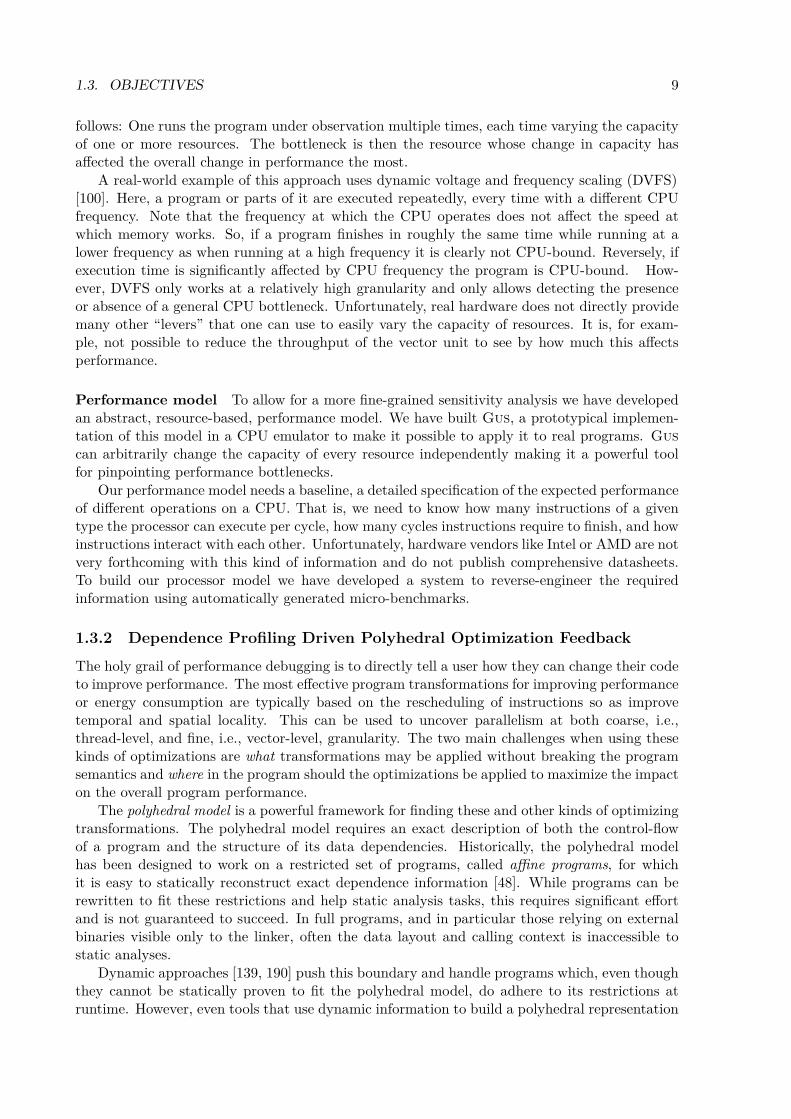
Performance model To allow for a more fine-grained sensitivity analysis we have developedan abstract, resource-based, performance model. We have built Gus, a prototypical implemen-tation of this model in a CPU emulator to make it possible to apply it to real programs. Guscan arbitrarily change the capacity of every resource independently making it a powerful toolfor pinpointing performance bottlenecks.
Our performance model needs a baseline, a detailed specification of the expected performanceof different operations on a CPU. That is, we need to know how many instructions of a giventype the processor can execute per cycle, how many cycles instructions require to finish, and howinstructions interact with each other. Unfortunately, hardware vendors like Intel or AMD are notvery forthcoming with this kind of information and do not publish comprehensive datasheets.To build our processor model we have developed a system to reverse-engineer the requiredinformation using automatically generated micro-benchmarks.
1.3.2 Dependence Profiling Driven Polyhedral Optimization Feedback
The holy grail of performance debugging is to directly tell a user how they can change their codeto improve performance. The most effective program transformations for improving performanceor energy consumption are typically based on the rescheduling of instructions so as improvetemporal and spatial locality. This can be used to uncover parallelism at both coarse, i.e.,thread-level, and fine, i.e., vector-level, granularity. The two main challenges when using thesekinds of optimizations are what transformations may be applied without breaking the programsemantics and where in the program should the optimizations be applied to maximize the impacton the overall program performance.
The polyhedral model is a powerful framework for finding these and other kinds of optimizingtransformations. The polyhedral model requires an exact description of both the control-flowof a program and the structure of its data dependencies. Historically, the polyhedral modelhas been designed to work on a restricted set of programs, called affine programs, for whichit is easy to statically reconstruct exact dependence information [48]. While programs can berewritten to fit these restrictions and help static analysis tasks, this requires significant effortand is not guaranteed to succeed. In full programs, and in particular those relying on externalbinaries visible only to the linker, often the data layout and calling context is inaccessible tostatic analyses.
Dynamic approaches [139, 190] push this boundary and handle programs which, even thoughthey cannot be statically proven to fit the polyhedral model, do adhere to its restrictions atruntime. However, even tools that use dynamic information to build a polyhedral representation

10 CHAPTER 1. INTRODUCTION
still face a number of problems. The main difficulty being how to model applications that includesome non-affine dependencies and memory accesses in otherwise affine code To address thisdifficulty existing dynamic polyhedral approaches either use overly pessimistic approximationsand lose information [199] or do not scale [112, 171].
Data-dependence driven polyhedral optimization feedback We have developed Mickey,a dynamic data-dependence profiler that builds a rich polyhedral IR from traces. Mickey workson compiled binaries and provides feedback on the applicability and profitability of polyhedralloop transformations. It can scale to real-life applications thanks to a safe, selective over-approximation mechanism for partially irregular data dependencies and iteration spaces.
Polyhedral interprocedural IR Mickey’s polyhedral IR encodes both the dynamic ex-ecution of a program’s instructions as well as its data dependencies. This IR captures theinterprocedural loop nesting structure of a program in a form that is amenable to analysis bya polyhedral optimizer. It not only captures data dependencies across multiple loops but also,possibly recursive, procedure calls.
Linear time polyhedral trace compression To construct the polyhedral IR from a pro-gram’s execution, we have developed the folding algorithm, an efficient trace compression algo-rithm. This technique was inspired by existing polyhedral trace compression techniques [112,171], with the notable difference that it uses the geometry of iteration spaces which allows it toscale to large irregular programs. The folding algorithm also detects which instructions in a pro-gram are used to increment loop counters and finds strides in memory accesses by building scalarevolution expressions (SCEVs) [161, 213] for loads, stores and integer arithmetic instructions.
1.3.3 Contributions
To summarize, in this thesis we present the following contributions:• A sensitivity based analysis tool to detect performance bottlenecks in programs (Chap-
ter 3).• A tool to reverse engineer performance characteristics of instructions on modern x86 CPUs
(Section 3.5).• A data-dependence based profiling tool that provides high-level optimization feedback
(Chapter 4).• An interprocedural polyhedral intermediate representation (Section 4.4).• A linear time polyhedral trace compression algorithm to construct this representation
(Section 4.5.5).
1.4 Structure of the ThesisThis thesis consists of four main chapters and is organized as follows:
• Chapter 2 gives a technical description of the dynamic binary instrumentation platformwe developed for our work. It contains mostly technical details and can be skipped on afirst read.
• Chapter 3 describes the bottleneck analysis algorithm and the CPU performance reverse-engineering tool.
• Chapter 4 presents our data dependence driven tool for giving optimization feedback.• Finally, Chapter 5 concludes the thesis, giving a summary of the contributions and per-
spectives on possible future work.

Chapter 2Dynamic Binary Instrumentation with
QEMU
Contents2.1 QEMU . . . . . . . . . . . . . . . . . . . . . . . . . . . . . . . . . . . . . . . . 122.2 The Tiny Code Generator . . . . . . . . . . . . . . . . . . . . . . . . . . . . . 132.3 The TCG Plugin Infrastructure . . . . . . . . . . . . . . . . . . . . . . . . . . 162.4 Execution Tracing with QEMU . . . . . . . . . . . . . . . . . . . . . . . . . . 19
2.4.1 Control-flow tracing . . . . . . . . . . . . . . . . . . . . . . . . . . . . 202.4.2 Data Dependence Tracing . . . . . . . . . . . . . . . . . . . . . . . . . 272.4.3 Value tracing . . . . . . . . . . . . . . . . . . . . . . . . . . . . . . . . 28
2.5 Evaluation of the Overhead of Plugins . . . . . . . . . . . . . . . . . . . . . . . 282.6 Related Work . . . . . . . . . . . . . . . . . . . . . . . . . . . . . . . . . . . . 292.7 Conclusion and Perspectives . . . . . . . . . . . . . . . . . . . . . . . . . . . . 34
11

12 CHAPTER 2. DYNAMIC BINARY INSTRUMENTATION WITH QEMU
Preliminary note: this chapter is very technical and describes the internals of someanalyses on which techniques presented later in the thesis are based. This chapterdoes not necessarily present any novel approaches by itself, but gives the generaltechnical context of the thesis. As a consequence, it is possible to skip it at firstreading.
This chapter describes the internals of the QEMU CPU emulator and TCG plugin infras-tructure (TPI), an infrastructure for building dynamic binary program analysis tools based onQEMU. It also gives a general overview over the field of dynamic binary translation and alsoshow cases a number of analyses we have implemented using TPI. The chapter is intended toboth show how TPI works in practice as well as to present some basic techniques which are usedlater throughput the thesis.
2.1 QEMU
QEMU [17, 166] is a processor emulator based on dynamic binary translation. That is, itallows running programs written for one CPU architecture on a different CPU architecture.QEMU only reproduces the functional aspects of a CPU, meaning it emulates the instructionset architecture (ISA). It does not, however, match the non-functional microarchitectural detailsof an architecture such as timing, cache effects, or speculative execution.
Vanilla QEMU only allows running programs on a different CPU architecture than the onethey where written for. ONe can, for example, run a program compiled for a 64 bit x86 CPU ona 32 bit ARM computer, and vice versa. The machine code of the emulated program is translatedand run as native machine code for the architecture QEMU is running on. This makes emulationrelatively fast compared to interpreter based systems like gem5 [23].
For the purposes of this work we use a modified version of QEMU [84] that includes TPIwhich makes it possible to alter programs as they execute. We chose to use QEMU for thissince it can emulate a plethora of different CPU architectures and supports all major operatingsystems (OSs), including GNU/Linux, *BSD, Mac OS X and Windows. QEMU furthermore hasa simple, more or less architecture independent, intermediate representation (tiny code generator(TCG) IR). This makes it easy to write analysis tools that work at the level of machine codebut are still portable across different system. Details of how this works will be presented inSection 2.3, for now we will focus on presenting QEMU itself.
QEMU internally uses the following terminology, which we will reuse:• Host CPU/OS: the CPU and OS on which QEMU is running.• Guest program/OS: the program/OS you run inside QEMU.• Guest CPU or virtual CPU: The state of a CPU core as emulated by QEMU.QEMU can be run under two different modes: full system mode and user mode. Full system
mode emulates a whole computer, including the CPU and peripherals such as network cards orhard disks. This means a whole operating system, including a kernel, is running on the simulatedmachine inside QEMU. This is similar to what sytems like VirtualBox [57] or Bochs [126] provide,but they can only run x86 programs on x86 hosts. User mode runs a single user space processand translates the machine code from the guest ISA to the host ISA. Under this mode QEMUruns a program compiled for one CPU architecture as a process in an operating system foranother architecture. To make this possible QEMU translates system calls to the ABI of thehost kernel. All the work done in this thesis has used QEMU in user mode, but it could easilybe modified to support full system mode.

2.2. THE TINY CODE GENERATOR 13
2.2 The Tiny Code Generator
The TCG is the component of QEMU responsible for translating guest machine instructions tohost machine instructions. TCG is essentially a just-in-time compiler (JIT) compiler that takesreal machine code as input instead of byte code.
Since TCG is a JIT it translates a program piece by piece at runtime. As a consequence theexecution of code and its compilation are interleaved. That is, when a program tries to run asequence of guest instructions the emulated guest CPU is halted and TCG translates the codeto host instructions. Once TCG has finished compiling the emulation resumes by executing thenew native code on the host. In the following we will refer to the moments when emulation ishalted and TCG takes over as translation time and the moments when the code of the emulatedprogram is running as execution time.
TCG is essentially a trace based JIT [150]. That is to say, it does not translate wholeprograms or functions at a time but only works on small linear sequences of guest instructionscalled trace blocks. These trace blocks are formed from the guest program using a very simplemechanism. Whenever the guest CPU executes an instruction that has not been translated yeta new trace block is started. This first instruction of the trace block is referred to as its entry.QEMU then parses the guest instructions following the entry until it hits a branch instruction1. The final trace block then contains the entry, the terminating branch and all instructions inbetween. Note that instructions in the guest program that are never executed are also nevertranslated by TCG.
Since we are using QEMU in user mode kernel space instructions are not visible to TCG.When guest code performs a system call this is translated to a corresponding system call on thehost system. Instructions that perform a system call, i.e. sysenter and syscall on x86, still areconsidered trace block terminators. They do not, however, change the program counter of thevirtual CPU and the emulated execution simply falls through to the next guest instruction oncethe system call has finished.
Due to the way trace blocks are constructed they are very similar the basic blocks of theguest binary. That is
• a trace block has only one entry,• a trace block has only one exit, 2
• and consequently once a trace block has been entered all instructions in it are executedexactly once, in order.
The important difference to the original guest basic blocks is that trace blocks can overlap,i.e. that a given guest instruction can be contained in multiple trace blocks. This happens forexample if guest code branches to an instruction which is in the middle of another trace blockthat has already been translated. The only restriction being that an instruction can only be theentry for one trace block. An illustrative example showing how a piece of code is divided intobasic blocks and trace blocks can be seen in Figure 2.1.
Internally, TCG does not directly translate the guest instructions in a trace block to hostinstructions. Instead it first translates traces to a more machine independent IR. Finally, theIR is then translated to machine instructions that can be executed directly on the host. Thesequence instructions generated for a whole trace block is called a translation block (TB). Thisprocess is illustrated in Figure 2.2a.
TCG IR consists of simple RISC-like instructions working on registers and memory addresses.The IR distinguishes between registers of the simulated guest CPU and virtual registers in the
1QEMU also terminates trace blocks before it finds a branch if the trace block is too long or if the guestinstructions would span two pages in memory
2like many other compilers QEMU is actually not very strict about this. Instructions that can fault, likememory accesses or division, are not considered block terminators.

14 CHAPTER 2. DYNAMIC BINARY INSTRUMENTATION WITH QEMU
A: test %rsi, %rsi
jz C
B: imul (%rsi), %rax
sub $8, %rsi
C: add %rdx, %rax
ret
(a) original program
A: test %rsi, %rsi
jz C
B: imul (%rsi), %rax
sub $8, %rsi
C: add %rdx, %rax
ret
(b) basic blocks
A: test %rsi, %rsi
jz C
B: imul (%rsi), %rax
sub $8, %rsi
C: add %rdx, %rax
ret
C: add %rdx, %rax
ret
(c) trace blocks
Figure 2.1 – A piece of x86 assembler in AT&T syntax and how it is divided into basic blocks and traceblocks. Note that B: and C are split into two basic blocks since C is the target of a branch. However, B andC form a single trace block since B does not end in a branch. There is a separate trace block containingonly C which is created when the branch at the end of A is taken.
trace block
guest ISA(x86, ARM, …)
translation block (TB)
TCG IR
compiled TB
host ISA(x86, ARM, …)
decode compile
(a) Illustration of how TCG translates guest code to host code.
init guest PClook up TB for
guest PC
decode trace
block
compile TBexecute host machine code
for TB
(updates guest PC)
TB not found
TB found
(b) Main emulator loop of QEMU.
Figure 2.2 – High-level view of CPU emulation with QEMU.
IR used to hold intermediate values. It also uses distinct instructions to access memory of theguest CPU and the host memory used for QEMU’s internal data structures. There are likewisedistinct opcodes for branches inside a TB and for branches that leave the current TB.
TCG IR is typed using a very simple type system. The only types are 32 and 64 bit integersand pointers. Very recently, 128 and 256 bit vector types where added too. But notably thereare no types to represent floating point values.
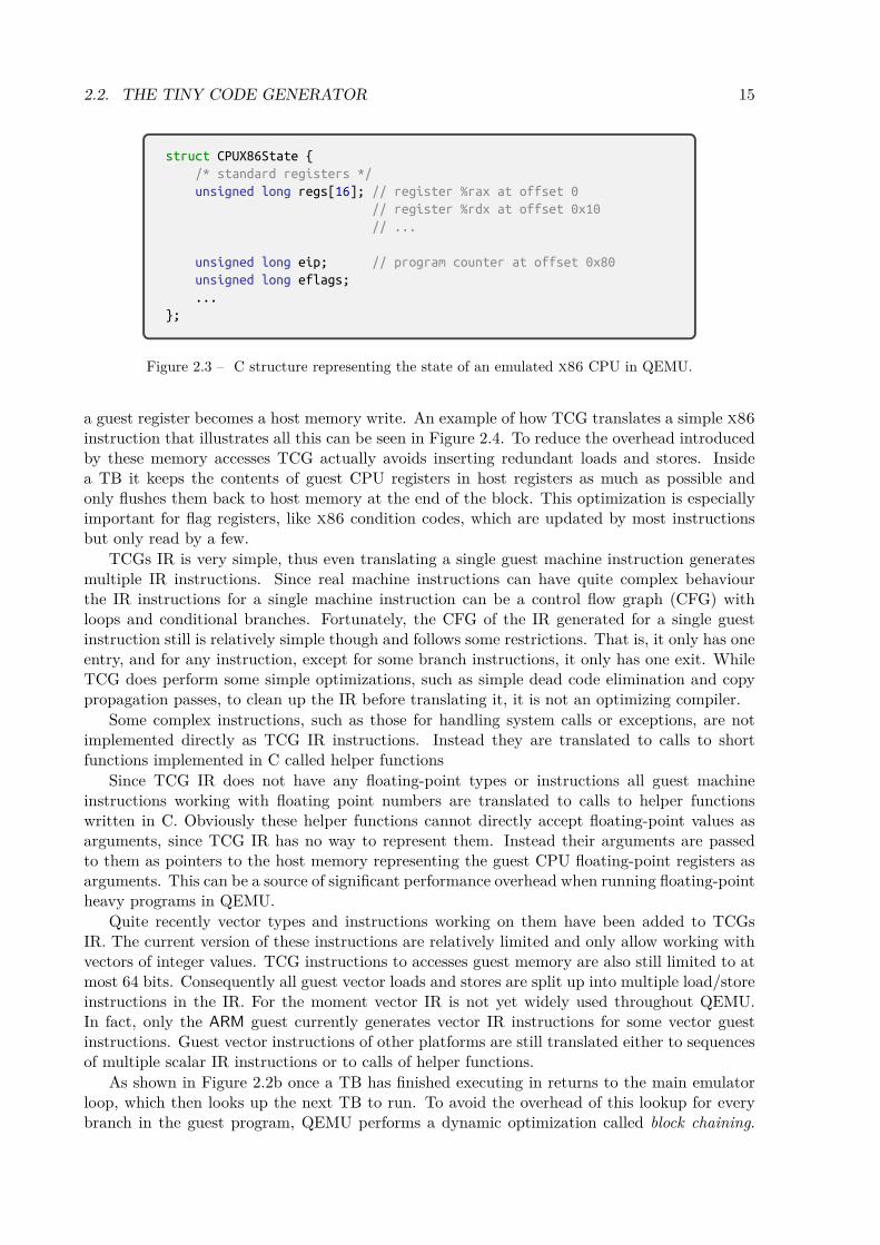
During emulation the state of the guest CPU is represented as an object in the heap ofthe QEMU process. For example, an x86 CPU has 16 general purpose 64 bit registers and sothe CPU object for x86 guests contains an array with 16 64 bit integers. An excerpt of thedefinition of the structure used to represent x86 guest CPUs can be seen in Figure 2.3. Sincethe registers of the guest CPU reside in host memory every use of a register in a guest program istranslated to a host memory access reading a field of the guest CPU object. Likewise, a write to
2.2. THE TINY CODE GENERATOR 15
struct CPUX86State {
/* standard registers */
unsigned long regs[16]; // register %rax at offset 0
// register %rdx at offset 0x10
// ...
unsigned long eip; // program counter at offset 0x80
unsigned long eflags;
...
};
Figure 2.3 – C structure representing the state of an emulated x86 CPU in QEMU.
a guest register becomes a host memory write. An example of how TCG translates a simple x86instruction that illustrates all this can be seen in Figure 2.4. To reduce the overhead introducedby these memory accesses TCG actually avoids inserting redundant loads and stores. Insidea TB it keeps the contents of guest CPU registers in host registers as much as possible andonly flushes them back to host memory at the end of the block. This optimization is especiallyimportant for flag registers, like x86 condition codes, which are updated by most instructionsbut only read by a few.
TCGs IR is very simple, thus even translating a single guest machine instruction generatesmultiple IR instructions. Since real machine instructions can have quite complex behaviourthe IR instructions for a single machine instruction can be a control flow graph (CFG) withloops and conditional branches. Fortunately, the CFG of the IR generated for a single guestinstruction still is relatively simple though and follows some restrictions. That is, it only has oneentry, and for any instruction, except for some branch instructions, it only has one exit. WhileTCG does perform some simple optimizations, such as simple dead code elimination and copypropagation passes, to clean up the IR before translating it, it is not an optimizing compiler.
Some complex instructions, such as those for handling system calls or exceptions, are notimplemented directly as TCG IR instructions. Instead they are translated to calls to shortfunctions implemented in C called helper functions
Since TCG IR does not have any floating-point types or instructions all guest machineinstructions working with floating point numbers are translated to calls to helper functionswritten in C. Obviously these helper functions cannot directly accept floating-point values asarguments, since TCG IR has no way to represent them. Instead their arguments are passedto them as pointers to the host memory representing the guest CPU floating-point registers asarguments. This can be a source of significant performance overhead when running floating-pointheavy programs in QEMU.
Quite recently vector types and instructions working on them have been added to TCGsIR. The current version of these instructions are relatively limited and only allow working withvectors of integer values. TCG instructions to accesses guest memory are also still limited to atmost 64 bits. Consequently all guest vector loads and stores are split up into multiple load/storeinstructions in the IR. For the moment vector IR is not yet widely used throughout QEMU.In fact, only the ARM guest currently generates vector IR instructions for some vector guestinstructions. Guest vector instructions of other platforms are still translated either to sequencesof multiple scalar IR instructions or to calls of helper functions.
As shown in Figure 2.2b once a TB has finished executing in returns to the main emulatorloop, which then looks up the next TB to run. To avoid the overhead of this lookup for everybranch in the guest program, QEMU performs a dynamic optimization called block chaining.

16 CHAPTER 2. DYNAMIC BINARY INSTRUMENTATION WITH QEMU
When QEMU dynamically detects that a TB always branches to the same successor it patchesa jump instruction into the host machine code for the TB. So, instead of exiting to the mainemulator loop the first TB will directly branch to the code of the successor TB. This optimizationallows QEMU to spend most of its time in generated machine code and to only exit to the mainloop to translate new trace blocks or handle special events like interrupts
In user mode QEMU has spawns one OS thread per thread in the guest program where eachOS thread has its own virtual CPU object. Therefore, the guest program can truly execute codeconcurrently. To ensure that the memory ordering rules of the guest ISA are respected by thehost processor TCG inserts special memory barrier instructions wherever necessary [58]. Dueto the way threads are emulated a guest CPU will have has at most as many cores runningsimultaneously as the host CPU. An accurate simulation of a highly parallel guest architectureon a less parallel host is therefore not possible.
Examples of how QEMU translates some simple x86 instructions to TCG IR and then backto x86 code are shown in Figures 2.4, 2.5 and 2.6.
input x86 code# <OPCODE> <SRC1>, <DST>
# Copy contents of %rax to %rdx
mov %rax, %rdx
TCG IR# <OPCODE> <DST>, <SRC1>, <SRC2>
# No-op that signals the start of a
# new guest instruction
insn_start <PC of guest instruction>
# Copy contents of guest register
# %rax to virtual register tmp0
#
#
mov_i64 tmp0, rax
# Copy contents of virtual register
# tmp0 to guest register %rdx
#
#
mov_i64 rdx, tmp0
generated x86 code# <OPCODE> <SRC1>, <SRC2 and/or DST>
# host register %r14 contains a
# pointer to the guest CPU object.
# (CPUX86State as shown in Figure 2.3)
# Copy contents of guest register %rax
# to virtual register tmp0
# (guest register %rax is stored at
# offset 0 of the guest CPU struct)
mov (%r14), %rbp
# Copy contents of virtual register
# tmp0 to guest register %rdx
# (guest register %rdx is stored at
# offset 0x10 of the guest CPU struct)
mov %rbp, 0x10(%r14)
Figure 2.4 – TCG IR and x86 machine code generated to emulate an x86 mov instruction. Note thatthe operand order in x86 and TCG IR is reversed.
2.3 The TCG Plugin InfrastructureAs mentioned before the work presented in this thesis is not based on the main version of QEMU,but on a modified version [84, 85]. This modified QEMU has a mechanism for loading plugins,called the TCG plugin infrastructure (TPI), that can both observe and alter the translationprocess of TCG. To instrument a binary a plugin injects TCG IR instructions into TBs beforethey get translated back to host machine code. Since plugins operate at the IR level and notat the machine code level it is relatively easy to port plugins so they work with different guest

2.3. THE TCG PLUGIN INFRASTRUCTURE 17
input x86 code# <OPCODE> <SRC1>, <SRC2 & DST>
# %rdx = *(%rax) + %rdx
add (%rax), %rdx
TCG IR# <OPCODE> <DST>, <SRC1>, <SRC2>
# No-op that signals the start of a
# new guest instruction
insn_start <PC of guest instruction>
# tmp0 = guest.rax
#
#
mov_i64 tmp0, rax
# tmp1 = *tmp0
# little-endian quad-word (64-bit) load
qemu_ld_i64 tmp1, tmp0, LEQ, 0
# tmp2 = guest.rdx
#
#
mov_i64 tmp2, rdx
# tmp1 = tmp1 + tmp2
add_i64 tmp1, tmp1, tmp2
# guest.rdx = tmp1
mov_i64 rdx, tmp1
generated x86 code# <OPCODE> <SRC1>, <SRC2 and/or DST>
# host register %r14 contains a
# pointer to the guest CPU object.
# (CPUX86State as shown in Figure 2.3)
# host.rbp = guest.rax
# (guest register %rax is stored at
# offset 0 of the guest CPU struct)
mov (%r14), %rbp
# host.rbx = *(host.rbp)
# little-endian quad-word (64-bit) load
mov (%rbp), %rbx
# host.r12 = guest.rdx
# (guest register %rdx is stored at
# offset 0x10 of the guest CPU struct)
mov 0x10(%r14), %r12
# host.r12 = host.rbx + host.r12
add %rbx, %r12
# guest.rdx = host.r12
mov %r12, 0x10(%r14)
Figure 2.5 – TCG IR and x86 machine code generated to emulate an x86 add instruction (the IR toupdate the guest status flag register is omitted). Note that the operand order in x86 and TCG IR isreversed.
CPU architectures. Simple plugins whose behaviour does not depend on the exact semantics ofguest instructions can work with multiple different guest ISA without any modification.
Even though a plugin can insert arbitrary code into the guest program the bulk of ourinstrumentation is not in TCG IR, but in C and C++. Instead of generating large amountsof IR we insert only small snippets that call the instrumentation functions. Even though thisincurs some overhead we have chosen this approach to speed up the development process, sinceit is much easier to write in C/C++ than in the low level TCG IR.
Certain features of the design of QEMU and TCG incidentally work together to ease thedevelopment of plugins. TCG IR enforces a certain separation between host memory and guestmemory, since it uses different opcodes to work with the one or the other. This means thatthe IR emitted can freely use separate virtual registers and does not have to take care notto accidentally clobber resources of the guest program. Guest programs also have no way ofaccessing the registers and memory of the plugin, meaning a faulty guest cannot cause faultsin the emulator. Furthermore, temporary registers in TCG IR are distinct from guest machineregisters, meaning one can freely insert code at any place without having to spill or restorevalues in and out of memory explicitly. TCGs register allocator automatically takes care of this.

18 CHAPTER 2. DYNAMIC BINARY INSTRUMENTATION WITH QEMU
input x86 code# jump to code at address 0xCAFEBABE
jmp 0xCAFEBABE
TCG IR# <OPCODE> <DST>, <SRC1>, <SRC2>
# No-op that signals the start of a
# new guest instruction
insn_start <PC of guest instruction>
# virtual register 'env' contains a
# pointer to the guest CPU object.
# (CPUX86State as shown in Figure 2.3)
# no-op.
# can later be patched for TB linking
goto_tb $0x0
# guest.eip = 0xCAFEBABE
# (guest program counter is stored at
# offset 0x80 of the guest CPU struct)
movi_i64 tmp3, $0xCAFEBABE
st_i64 tmp3, env, $0x80
# exit TB, branch back to QEMU code
exit_tb ...
generated x86 code# <OPCODE> <SRC1>, <SRC2 and/or DST>
# host register %r14 contains a
# pointer to the guest CPU object.
# (CPUX86State as shown in Figure 2.3)
# no-op
# can later be patched for TB linking
xchg %ax,%ax
jmp label
label:
# guest.eip = 0xCAFEBABE
# (guest program counter is stored at
# offset 0x80 of the guest CPU struct)
mov 0xCAFEBABE, 0x80(%r14)
# exit TB, branch back to QEMU code
lea ..., %rax
jmp <QEMU-interpreter-loop>
Figure 2.6 – TCG IR and x86 machine code generated to emulate a x86 jmp instruction. Note that theoperand order in x86 and TCG IR is reversed.
A TPI plugin is simply a shared library which QEMU loads into memory on startup, beforeit even starts emulating the guest program. TPI offers a C API allowing plugins to registercallback functions which are then called whenever certain events occur. Most of these events arerelated to the translation of guest instructions to TCG IR. There are, for example, events thatsignal that TCG has started or finished constructing a new TB, and also events that signal thatTCG has started or finished decoding a guest machine instruction. Whenever such a callback iscalled the plugin can then choose to insert new IR instructions into the TB, or alter the existingones. A short excerpt of the plugin API is shown in Figure 2.7
TCG decodes trace blocks, i.e., it generates all IR instructions in a TB, in one pass. Virtualregisters are not in static single assignment (SSA) form [174], and instead are reused as muchas possible to reduce memory consumption of TCG itself during translation. Consequently, aTPI plugin written using only callbacks must emit its instrumentation directly as TCG emitsits IR or take care not to clobber virtual registers. As TPI only provides this event based APIinstrumentation plugins have to be written as a state machine or in continuation passing style.
Since TCG IR generates multiple IR instructions even for the simplest guest instructionwriting plugins that maintain state across a TB can quickly become quite tedious. To makewriting plugins easier we have developed a thin C++ API wrapper around the original TPI APIthat allows working with TCG IR in a more straightforward fashion. It allows plugins to work

2.4. EXECUTION TRACING WITH QEMU 19
struct TPIOpCode; // a single TCG IR instruction
struct Translation_Block;
/// Object representing the state of a plugin.
/// Contains callbacks that will be called by TPI.
struct TCGPluginInterface {
// Called whenever TCG is about to start decoding a new trace block.
// IR for trace will be stored in 'tb'.
void (*before_decode_first_instr)(const TCGPluginInterface *tpi,
const TranslationBlock *tb);
/// Called whenever TCG has finished decoding a trace block.
void (*after_decode_last_instr)(const TCGPluginInterface *tpi,
const TranslationBlock *tb);
/// Called whenever TCG is about to decode the next instruction of
/// the current trace block.
void (*before_decode_instr)(const TCGPluginInterface *tpi, uint64_t pc);
/// Called whenever TCG has inserted a new IR instruction into
/// the current translation block.
void (*after_gen_opc)(const TCGPluginInterface *tpi, const TPIOpCode *opcode);
...
};
Figure 2.7 – Core events of the TPI C API
with the IR for an entire TB at once and to perform multiple passes over the IR and to insertcode at any point in the TB. We have also wrapped TCGs routines for allocating and freeingvirtual registers so a plugin author does not have to worry about overwriting registers used bythe guest code itself.
TCG IR has control flow but does not directly represent basic blocks, it just has set_label
and branch to label instructions. Our IR layer also detects the basic blocks in a TB and makesit easy to iterate over successors and predecessors. However, the C++ TPI wrapper currentlydoes not allow altering the control flow of a TB, i.e. it cannot change jump targets and alsocannot insert or remove jumps.
2.4 Execution Tracing with QEMU
During this thesis we have developed different tools to perform high-level analyses on Executableand Linkable Format (ELF) [206] binaries. The input of these tools are traces of events describingdifferent aspects of the execution of a program. This section describes three TPI plugins wehave developed to trace a program’s control-flow, data-dependencies and integer computations.
On a side note, we want to point out that execution traces of real world programs canbecome extremely large. So large, in fact, that realistically we cannot store entire traces in files.This can be illustrated with a little thought experiment. A modern CPU runs at a frequencyof several GHz, meaning every second it can execute billions of instructions. When tracing asmall program that only runs for one second if one retains even only one byte of data for everyinstruction that is executed the resulting raw trace will already contain more than one gigabyteof data. Consequently, all plugins presented here are designed as libraries that produce streamsof events which can be treated directly in memory. If necessary, for example for debugging or

20 CHAPTER 2. DYNAMIC BINARY INSTRUMENTATION WITH QEMU
verification purposes, partial traces can still be stored to a file.
2.4.1 Control-flow tracing
The control-flow tracing plugin we have developed observes the branches executed in a programand has the goal of distinguishing local control-flow inside a function and calls and returnsbetween functions. This information can in turn be used to:
• Recover the interprocedural call graph (CG) and intraprocedural control flow graph (CFG)of a program and
• track the calling-context, that is a compact representation of the call stack, during execu-tion.
Since portability, across CPU architectures as well as across languages, was one of our mainconcerns we took great efforts to make our plugin independent of platform and language ABIs.It does not inspect the call stack and only uses basic assumptions about branch instructions ofa given architecture. This approach is also robust against of software stack unwinders as used,for example, for exception handling in C++.
The main problem with control-flow tracing is that, as mentioned earlier, binary machinecode is much less structured than source code. The plethora of high-level control flow found inprograms, like loops, conditionals, function calls, returns and exception handling, are all reduceddown to a small number of branch instructions. On x86, for instance, all normal control flow isimplemented using only call, ret, jmp and jcc. Hence, the machine code conflates at least somedifferent types of control flow by implementing them using the same instructions. Compilers canalso sometimes use different machine instructions to implement the same control flow constructdepending on they context are used in, e.g., replacing calls with a cheaper jmp where possible.This means our plugin has to be able to detect the intended purpose of a branch instructionfrom the instructions immediately surrounding it and branch target.
Since the plugin needs to be able to distinguish different forms of guest branch instructions itcannot work solely at the level of TCG IR. To make it easier to port the plugin between differentarchitectures the main part of the code works does not work directly with guest opcodes. Insteadwe map the different guest branch instructions to a reasonably small set of abstract terminatortypes shown in Figure 2.10. Thanks to this only a small part of the plugin that is responsiblefor categorizing guest instructions is architecture dependent. The majority of the code and alsoall the instrumentation we generate does not need to be changed to support new platforms.
In practice, local branches inside functions are mostly regular and easy to handle. The mainproblems arise when trying to handle calls and returns between functions. For example, the“normal” way to translate a function call in C is using the call instruction. But this is byfar not only way that function calls are actually implemented. The most commonly occurringalternative implementation, tail call optimization, which has already been mentioned, uses jmp
instructions instead, which are normally used for control-flow inside a function. But there arealso other, more exotic, ways to implement function calls. In highly hand optimized assemblycode, as can be found in the GNU C standard library, there are cases where a function calloccurs via fall-through, i.e., without any branch instructions. An example of this can be seen inFigure 2.8. Another reason why interprocedural control flow is more difficult to handle is that inmodern code bases using virtual function dispatch and function pointers or lambda expressionsindirect branches are much more common. In general it is not possible to statically detect thetarget of such indirect branches meaning we have no information about the target of the branchbefore actually executing the branch.
There are also cases where call instructions are used for other purposes than function calls.On pre 64 bit x86 CPUs there is no direct support for RIP relative addressing, which is necessaryfor writing position independent code. One idiom used to work around this is show in Figure 2.9.

2.4. EXECUTION TRACING WITH QEMU 21
0000000000149cd0 <__strcasecmp_ssse3>:
149cd0: f3 0f 1e fa endbr64
149cd4: 48 8b 05 e5 60 07 00 mov 0x760e5(%rip), %rax
149cdb: 64 48 8b 10 mov %fs:(%rax), %rdx
149cdf: 0f 1f 44 00 00 nopl 0x0(%rax, %rax, 1)
149ce4: 66 66 2e 0f 1f 84 00 data16 nopw %cs:0x0(%rax, %rax, 1)
149ceb: 00 00 00 00
149cef: 90 nop ⇐ fall-through!
0000000000149cf0 <__GI___strcasecmp_l_ssse3>:
149cf0: f3 0f 1e fa endbr64
149cf4: 48 8b 02 mov (%rdx), %rax
149cf7: f7 80 78 02 00 00 01 testl $0x1, 0x278(%rax)
149cfe: 00 00 00
149d01: 0f 85 d9 ba f5 ff jne a57e0 <__strcasecmp_l_nonascii>
149d07: 89 f1 mov %esi, %ecx
149d09: 89 f8 mov %edi, %eax
149d0b: 48 83 e1 3f and $0x3f, %rcx
149d0f: 48 83 e0 3f and $0x3f, %rax
... ... ...
Figure 2.8 – Example of a function call by fall-through. As seen in glibc 2.28.30 (Fedora 29) inx86 (AT&T syntax). __strcasecmp_ssse3 (an optimized version of strcasecmp using x86 SSSE3 [54]instructions) does not end in a branch instruction. Instead execution will always fall-through to__GI___strcasecmp_l_ssse3 (another optimized variant of strcasecmp).
call here
here: pop %rax
# %rax now contains the absolute address of `here'
Figure 2.9 – 32 bit x86 assembly code to obtain the value of the program counter (AT&T syntax).
It consists of a call instruction that jumps zero bytes away, that is, it only pushes the valueof the program counter in the stack and falls through to the next instruction Even though thisuses a call instruction it is not an actual function call and is never returned from.
On 32 bit ARM the program counter is a general purpose register that can be read andwritten by any instruction. Consequently any instruction can perform a branch by writing tothe program counter register. The standard return instruction on 32 bit ARM, for example, isactually just “pop pc”. I.e. to return one simply pops the return address directly from the stackinto the program counter.
In this work we do not use any technique to reconstruct the boundaries of functions [9, 15]. In-stead we rely on the ELF symbol table and DWARF Debug Information Format (DWARF) [205]debug information to detect the addresses and boundaries of functions. We also make the fol-lowing assumptions about functions:
1. All code for a function is located in a single, contiguous ELF symbol; that is, they containno holes.
2. Functions do not overlap; if they do we split them into multiple non-overlapping functions.Since we want to not only support the regular code patterns emitted by most compilers, butalso hand written assembly code we also assume that functions can have multiple entry points,i.e. a call to a function does not necessarily enter at its first instruction.
Unfortunately, the ELF symbol table and debug information do not necessarily contain

22 CHAPTER 2. DYNAMIC BINARY INSTRUMENTATION WITH QEMU
information for all functions in a binary. Static functions in C/C++, for example, which aren’tpart of a binary’s interface are usually not included in the symbol table. As we currently havenot implemented any algorithm for recovering functions from machine code we group all the coderegions for which we have no information into one big “unknown” function. Since unmarkedcode is usually spread out over the binary and the shared libraries it loads we allow this specialfunction to, unlike any other function, contain holes.
Given this model of functions is it is quite straightforward to distinguish the different typesof branches. All information that is required for this is:
• The type of the instruction the trace that performed the branch, i.e., whether it was acall or jump, etc., and
• whether the source and the destination of the branch are in the same or in differentfunctions.
The pseudo-code for calculating the branch type can be seen in Algorithm 2.1.Finally, to detect when branches occur in the guest it suffices to simply track whenever
execution enters a new TB. Since branch instructions always terminate their trace block weknow that if a new TB is entered a branch has been executed. The event object, which can beseen in Figure 2.10, generated for every branch simply records the TB the branch originatedfrom and the target of the branch. To implement this the control-flow tracing does two thingswhenever a new TB is translated:
• It allocates a descriptor object recording metadata for the TBs, and• it inserts a call to a helper function at the beginning of the TB, passing the metadata
object as an argument. This helper function will then emit a branch event every time theTB is executed.
Pseudo-code for this can be seen in Figure 2.11.There is one particular case, though, where instrumenting only the entry of a TB does not
suffice. When a function does not end in a branch but falls through to the next function afterit, the current TB will typically not be terminated at this transition. Instead, the generated TBwill contain instructions from both functions. In this case, we have to insert a call to a helperfunction between the two functions to emit a branch event whenever the fall-through occurs.Ordinary fall-throughs that do not leave their function do not require any special treatment andare handled the same as normal local branches.
Using this instrumentation we can capture nearly all forms of control flow. However, thereare two types that cannot be recovered this way, namely: the interprocedural control-flowtransfers that occur during stack unwinding, and the local fall-through branches from a call
site to the instruction following it. The control-flow tracing plugin post-processes the raw streamof events generated by the instrumentation to detect these cases and inserts appropriate events.Pseudo-code for this can be seen in Algorithm 2.2.
During stack unwinding, which is usually used to implement exception handling for languagessuch as C++, one or more call frames can be discarded without using return instructions. Sincewe store the return destination of every call on the shadow call stack we can detect when theexpected destination and the actual target do not match. In this case we pop off shadow stackframes, adding unwind edges to the CG as we go, until we find a matching return target. Note,that this only works if the call stack is used like a stack. Advanced uses of setjmp/longjmp orfully fledged continuations are not supported.
In most IRs used in compilers and analysis tools interprocedural and intraprocedural control-flow is strictly distinguished. For simplicity, function calls are furthermore not considered branchinstructions from the point of view of the control-flow inside a procedure. Instead a functioncall is simply modelled as a single instruction with complex effects followed by a fall-through tothe next instruction. QEMU, on the other hand, directly emulates the behaviour of the CPUand does not have any notion of local or non-local control-flow. Thus, the control-flow tracing

2.4. EXECUTION TRACING WITH QEMU 23
# types of different instructions that can terminate a TB
enum Terminator_Type:
JUMP, CALL, RETURN, OTHER
# different types of branches we can detect
enum Branch_Type:
# inside a function
LOCAL_JUMP,
# between functions
CALL, TAIL_CALL, UNWIND, RETURN
struct Block:
# unique ID for the function containing this block
function: Function_Id
# PC of first guest instruction in block
start: PC
# type of the last instruction in the block
terminator_type: Terminator_Type
struct Branch_Event:
src: Block
dst: Block
brtype: Branch_Type
Figure 2.10 – Event data structures used for control flow tracing.
instrumentation will only observe a call branch out of the current function and later a returnbranch from the called function to the instruction after the call. Without further treatment anyconsumer of the event stream that only looks at the local control-flow would wrongly believethat the function call never returned. Instead, the control-flow tracing plugin emits a syntheticfall-through event after every return as shown in Algorithm 2.2, line 28. We cannot simply insertthis fall-through branch statically after every call instruction since some calls actually do notever return.
We will now briefly describe two low-level analyses using the final stream of branch eventsproduced by the control-flow tracing plugin to compute higher level information. Chapter 4contains higher level applications that build on top of them.
2.4.1.1 CFG and CG Reconstruction
For the analyses proposed in thesis, as described in Chapter 4, we need as precise informationabout control-flow as possible. However, statically reconstructing the exact CFG and CG frommachine code from is considered, in general, undecidable due to, among other things, data-dependent branches and instruction punning. Instead of an approximate static analysis wechose to use a dynamic analysis, based on our tracing infrastructure described above, which canperfectly capture the control-flow of a given execution of a program. Since the stream of eventsalready distinguishes local branches and non-local control flow and contains both the source anddestination of every branch it is trivial to reconstruct the CFG and CG from it. The trade-offbeing that the information is partial, only covering the parts of the program that actually whereexecuted, and depend on the input data used.
A consequence of this is that our analysis does not, strictly speaking, recover the basicblocks of a program. Recall, that a basic block has only one entry, meaning that blocks have

24 CHAPTER 2. DYNAMIC BINARY INSTRUMENTATION WITH QEMU
1 # types defined in Figure 2.10
23 def detect_branch_type(src: Block, dst: Block) -> Branch_Type:
4 if src.terminator_type == CALL:
5 return CALL
6 elif src.terminator_type == JUMP:
7 if src.function == dst.function:
8 # NOTE: we do not distinguish self-recursive
9 # tail calls and local branches.
10 return LOCAL_JUMP
11 else:
12 return TAIL_CALL
13 elif src.terminator_type == RETURN:
14 return RETURN
15 else:
16 # system call or fall-through
1718 if src.function != dst.function:
19 # fall-through to another function.
20 return TAIL_CALL
21 else:
22 # fall-through end of block
23 return LOCAL_JUMP
Algorithm 2.1 – Distinguish calls, tail calls and local jumps.
to be split at branch targets. In machine code, though, we cannot recover the destinationof branch instructions and any instruction is a valid branch target. We however believe thattreating every instruction as a separate block would be overly conservative. As a final outputour analysis still constructs single entry-single exit blocks of instructions, but only considersbranch targets actually observed. We call these execution blocks since they correspond to thebasic blocks observed during execution. Execution blocks are constructed from trace blocks bysplitting the trace blocks seen during execution such that every instruction is contained in atmost one block.
To improve coverage of the guest program the control-flow reconstruction plugin does takeinto account the targets of direct conditional branches that are never taken. It only considersdirect branches though, since their targets can be computed statically even if they are not taken.
2.4.1.2 Calling-context tracking
The behaviour of any piece of code can vary wildly with the inputs and machine state, such ascache or branch predicator state, with which it is executed. Without a notion of context a profilercan not differentiate different executions of the same piece of code, possibly producing wildlymisleading results. Ammons et al. [7] have proposed the idea of context sensitive profiling whereinformation is not attached to a single static location in a program but to a path through theprogram. They also introduced the calling context tree (CCT) data structure, which encodespaths through the CG and makes it possible to track the dynamic calling context for eachfunction call. Examples of a CG and CCT are shown in Figure 2.12
We have implemented a QEMU plugin which uses our control-flow trace to compute thecalling contexts in which every instruction in a program executes. Note that, while the work ofAmmons et al. goes beyond tracking calling contexts, this section is only meant to illustrate an

2.4. EXECUTION TRACING WITH QEMU 25
# types defined in Figure 2.10
# global variable
previous_block = None
# callback that is invoked whenever a block is executed
def on_enter_translation_block(block: Block):
if previous_block != None:
brtype = detect_branch_type(previous_block, block) # Algorithm 2.1
emit Branch_Event(previous_block, block, brtype)
previous_block = block
(a) Pseudo-code for the helper function that raises the branch events.
input TCG IR
insn_start 0x401240
mov_i64 tmp1, rax
mov_i64 tmp0, rdx
or_i64 tmp0, tmp0, tmp1
mov_i64 rdx, tmp0
...
instrumented TCG IRmov_ptr tmp0, <Block object for TB>
call on_enter_translation_block(tmp0)
insn_start 0x401240
mov_i64 tmp1, rax
mov_i64 tmp0, rdx
or_i64 tmp0, tmp0, tmp1
mov_i64 rdx, tmp0
...
(b) Example of generated instrumentation in TCG IR.
Figure 2.11 – Code inserted to trace raw branch events.
M
D
A
B C
(a) call graph
M
A
B
M
D
A
C
M
D
C
(b) Some example call paths
M
DA
A
B
C
C
(c) calling context tree
Figure 2.12 – Example call graph and associated calling context tree.
application of control-flow tracing and focuses on our implementation of CCTs in QEMU. Sec-tion 4.4 will present an extended algorithm that also takes local control-flow inside of functionsinto account.
Our CCT implementation is, in essence, a trie [59, 27] encoding the set of call stacks thatwhere live during a program’s execution. Every node in the CCT represents one call frameand stores the address of the instruction that performed the call and the address where the callshould return. The node data structure also contains an identifier of the function containingthe call instruction for easy reference. The children of a CCT node in turn correspond to all thefunctions that have been called while the call frame from that node was live. By furthermorestoring a parent pointer in every node of the CCT we can compactly represent a whole call stack

26 CHAPTER 2. DYNAMIC BINARY INSTRUMENTATION WITH QEMU
1 # Shadow call stack mirroring the real call stack of the guest.
2 call_stack: Stack<Call_Frame>
34 def on_branch(evt: Branch_Event):
5 if evt.type == CALL:
6 # Push shadow call frame on the call stack
7 call_stack.push({evt.src, ...});
8 # Forward call event
9 emit evt
10 elif evt.brtype == RETURN:
11 caller = call_stack.pop()
1213 if caller.return_target != evt.dst.start:
14 # Return did not go where it was supposed to due to
15 # an exception or longjmp.
16 # Unwind stack.
1718 while True:
19 caller = call_stack.pop()
20 if caller.return_target == evt.dst.start:
21 break
22 emit Unwind_Branch(caller)
2324 # emit the actual return event itself
25 assert caller.return_target == evt.dst.start
26 emit Return_Branch(caller, evt)
2728 # fall-through from TB terminated by call.
29 if caller.function == evt.dst.function:
30 emit Local_Branch(caller, evt.dst)
31 else:
32 emit Tail_Call(caller, evt.dst)
33 else:
34 ...
Algorithm 2.2 – Code to handle function returns and exception unwinding.
with a single node reference.
Note that this version the CCT has no bound on the depth of the tree. With recursion thedepth of the CCT will in fact grow proportionally with the depth of the recursion. It also doesnot contain any information about local control-flow inside of functions. The original version,developed by Ammons et al., does in fact bound the depth of the tree and also encodes localflow information. However, it only achieves this by ignoring cycles in the CG and CFG. Wehave developed an extension of the CCT that captures both recursive call paths as well as loopsinside of functions which will be described in Section 4.4.
In the following we will use references to CCT nodes plus the address of an instruction asinstruction identifier. Including a CCT node in the identifier allows us to distinguish differentdynamic executions of an instruction.

2.4. EXECUTION TRACING WITH QEMU 27
2.4.2 Data Dependence Tracing
The goal of data dependence tracing is to discover pairwise data dependencies between instruc-tions. For our purposes we define that a data-dependence occurs when an instructions readsdata produced by another instruction. Note that we also distinguish different dynamic execu-tions of the same instruction. That is if an instruction is executed in a loop we will emit newdata dependence events every iteration. While there are powerful static techniques to calculatedata dependencies, like the polyhedral model, they only produce accurate results for a highlyrestricted class of programs. In order to be able to produce precise results for general programswe chose, as we did for control-flow tracing, to use a dynamic approach.
To detect dynamic data dependencies in programs we use shadow memory [45, 154, 229]. Ashadow memory is a data structure that records a piece of information for each storage locationused in a program. For dependency tracking the information is usually an identifier for the lastinstruction that modified that location. Now, whenever an instruction reads data from a storagelocation, i.e. performs a read from memory or a register, we can find the producer of that datain the shadow memory.
Our implementation of a shadow memory works at byte granularity, meaning that a 4-bytewrite will update four shadow memory cells and a 4-byte read will look at four shadow memorycells. We actually group entries of the shadow memory into shadow pages, similar to how normalmemory is split into pages. These pages are stored in a search tree allowing for quick retrieval.Grouping cells together allows us to exploit the locality of memory accesses in two ways:
1. Even though a n-byte memory access touches n shadow cells all these cells are usuallylocated on the same page. This means that, even though we work at a byte granularity,we only have to perform on lookup once per memory access. At most two, if the accessspans two pages. A shadow page itself is just a large array and the actual reads or updatesof shadow cells can be performed directly.
2. We have implemented a small and fast shadow page cache [229] which speeds up repeatedaccesses to the same page.
Our library is not only able to trace data dependencies via memory, but also via registersusing a shadow register file. Here the mapping from guest CPU registers to shadow registers ismuch more straightforward, since the registers used by a machine instruction can be determinedstatically and also because the number of registers in a CPU is usually quite small. The shadowregister file is implemented as an array with one entry for every guest CPU register. Forsimplicity we do not consider register aliasing. That is, a write or read of a register is alwaysassumed to access the whole register.
An attentive reader might have noticed that we only track read-after-write (RAW), or true,dependencies. The plugin could easily be extended to also track write-after-write (WAW), oroutput, dependencies. For the most we chose not to do so because our current applications do notrequire it and because it would only generate unused events. Tracking write-after-read (WAR)or read-after-read (RAR) dependencies directly would be more complicated and costly since itrequires updating the shadow memory at reads. If necessary WAR and RAR dependencies canbe recalculated as a post-pass from the RAW and WAW dependence information.
To reduce the size of traces and ease later analysis our shadow memory implements a simpleform of dynamic copy propagation. This mechanism applies whenever the instrumenting data-copying instructions which only move data between storage locations without modifying it. Theinstrumentation inserted to update the shadow memory for these instructions works slightlydifferent. If a dynamic execution of a copy instruction only reads data produced by a singleother instruction the identifier recorded in the shadow memory cell for the destination of the copyis not that of the copy instruction but that of the actual producer. This propagation mechanismis designed to, among other things, filter out spill code inserted by compilers to store and load the

28 CHAPTER 2. DYNAMIC BINARY INSTRUMENTATION WITH QEMU
contents of registers to and from the stack. The idea being that instructions that don’t computeanything and only move data around are usually not interesting for dependence analysis. Sincethe exact definition of what constitutes a pure data copy is a bit vague and can vary along withdifferent use cases. Our shadow memory can thus be configured to also consider instructionsthat perform integer truncation, sign-extension or conversion between integers and floating pointnumbers as copy operations.
For x86 guests we also detect classical dependence breaker idioms as documented by Inteland extensively used by compilers. These idioms are instructions used as hints by compilers tobreak false dependence chains via registers. Take for example the instruction xor %rax, %rax,which performs a bitwise xor on the contents of the register %rax and stores the result back into%rax. The result of this instruction does not depend on the contents of %rax, it will always set%rax to 0, and it does not create a data dependence on whoever last wrote to %rax.
Our current implementation of shadow memory does not support concurrent accesses bymultiple threads from the guest program. Consequently, our dependence tracking plugin canonly be used for serial programs.
2.4.3 Value tracing
The simplest form of tracing we have implemented is value tracing. The goal of value tracing isto capture any value architecturally computed by the guest program. That is any value writtento a guest CPU register or to guest memory. We also consider memory addresses that a guestprogram accesses as values, even if the addresses are calculated inside the instruction and notstored anywhere. Same as the control-flow and data dependence tracing we use this as part ofthe dynamic analysis presented in Chapter 4. As shown in that chapter we use these tracedvalues and addresses to detect loop iterators and regular memory access patterns.
The TPI value tracing plugin we have written generates one event for every guest instructionexecuted. For our purposes we actually do not consider every instruction, but only those thatproduce integral values and/or perform a memory access. Most branch, compare, floating pointor vector instructions are not considered here. The event contains an identifier for the instructionalong with space for one register sized value and one memory address. For instructions that donot generate a value, such as store instructions, we mark the value field as unused. Similarly,for instructions that do not access memory we mark the address field as unused. For simplicityan event can store at most one value and address each. In the rare case that an instructionsproduces more than one value or accesses more than one address we do not capture all thesevalues but instead mark the corresponding field in the event as unused.
2.5 Evaluation of the Overhead of PluginsIn this section we show the overhead incurred by running programs in QEMU with some of ourplugins. We also compare this to the slowdown of running the same programs in other binarytranslators.
To evaluate the overhead of our plugins we have used the latest revision (3.1) of the Rodiniabenchmark suite [42, 43]. As our tool-chain does not support multi-threaded applications yet,each benchmark is manually modified to turn into a single thread. It is then compiled usingGCC 8.1 using flags -g -O2 -msse3. We use -sse3 since QEMU does not yet have full supportany more recent vector instructions. The binary translators we used are QEMU version 3.1,Valgrind version 3.15.0 [155], and DynamoRIO version 7.1.0 [29]. All time measurements whereperformed on a single core of a Haswell i5-4590 CPU running at 3.3GHz.
We first evaluate the overhead of using QEMU-plugins as an instrumentation framework.For that purpose we compare the execution time in different contexts:

2.6. RELATED WORK 29
(time) (slowdown)
nati
ve
QE
MU
Val
grin
d
Dyn
amor
io
Din
ero
IV
Cac
hegr
ind
drca
ches
im
bftr
ace
shad
owm
emor
y
backprop 0.04s±0.0s 7.5x 8.8x 1.1x 455x 28x 373x 24x 63xbfs 1.1s±0.0s 5.8x 7x 0.5x 921x 50x 859x 40x 173xb+tree 1.1s±0.0s 5x 6.8x 0.1x 850x 40x 654x 38x 101xcfd 2.1s±0.0s 28x 5x 0.2x 475x 34x 419x 44x 132xheartwall 16.96s±0.1s 31x 11x 0.01x 608x 29x 464x 43x 90xhotspot 1.1s±0.0s 5x 5x 0.3x 573x 52x 537x 33x 167xhotspot3D 4.5s±0.0s 24x 8.5x 0.1x 725x 48x 607x 39x 164xkmeans 3.9s±0.0s 38x 12x 0.1x 807x 39x 611x 61x 181xlavaMD 4.1s±0.0s 38x 21x 3.7x 627x 44x 521x 54x 130xleukocyte 11.8s±0.0s 56x 20x 1.9x 819x 48x 587x 75x 174xlud 0.1s±0.0s 22x 11x 0.6x 804x 56x 732x 49x 170xmyocyte 0.002s±0.0s 24x 120x 22x 306x 157x 478x 82x 149xnn 0.01s±0.0s 8.9x 26x 3.7x 518x 57x 489x 41x 121xnw 0.1s±0.0s 2x 6.1x 0.7x 314x 19x 268x 9.8x 45xparticlefilter 0.3s±0.0s 32x 10x 0.2x 746x 39x 611x 62x 127xpathfinder 0.8s±0.0s 6.6x 6.4x 0.7x 758x 41x 686x 39x 132xsrad_v1 0.5s±0.0s 47x 6.8x 0.2x 416x 23x 308x 53x 100xsrad_v2 0.3s±0.0s 40x 10x 1.2x 401x 26x 307x 48x 88xstreamcluster 38.1s±0.3s 42x 7.4x 0.01x 473x 23x 357x 50x 102x
Table 2.1 – Overhead of profiling on the Rodinia benchmark suite: slowdown compared to nativeexecution (overhead = emulator time−native time
native time ). Times are averaged over ten runs.
1. We take the native execution time as a baseline.2. We evaluate raw execution time of different binary translators, i.e., without any instru-
mentation.3. We evaluate the overhead of doing basic memory profiling of those frameworks (Dinero
IV [66] for cache simulation under QEMU, cachegrind [152] for Valgrind, drcachesim forDynamoRIO).
4. We finally evaluate the overhead of CFG reconstruction plugin and a simple shadow-memory plugin that traces data dependencies between machine instructions.
Table 2.1 reports the slowdown compared to the native execution time on backprop (bench-mark used for our case study) and Rodinia (average values). We observe the following: Withoutany plugins Valgrind and QEMU run at roughly the same speed, while DynamoRio is muchfaster; Still as one could expect, the main source of overhead is the inserted instrumentationitself. Even a highly optimised cache simulator like Cachegrind incurs a close to 4x slowdowncompared to just running Valgrind by itself. The control-flow tracing plugin has a relativelylow overhead since it only inserts instrumentation at the beginning of every trace block. Theshadow memory plugin, on the other hand, has a substantially higher overhead.
As we can see from this table QEMU is clearly not the fastest binary translation system.However, as soon as we perform any significant instrumentation the overhead introduced of theinstrumentation clearly dominates the overhead of the binary translator.
2.6 Related Work
This section discusses some previous work related to binary instrumentation and also regardingthe applications thereof presented in this chapter.

30 CHAPTER 2. DYNAMIC BINARY INSTRUMENTATION WITH QEMU
QEMU based tools
Two projects closely related to our work are TEMU[193], part of the BitBlaze tool suite, andits successor DECAF [89]. Both of these tools implement a dynamic binary instrumentationinfrastructure based on QEMU. TEMU and DECAF can only run using QEMU’s full systemmode which emulates and observe a whole operating system. Like TPI, both offer a plugin APIwhich can be used to implement dynamic analyses. Their APIs, however, do not give pluginsdirect access to TCG IR. Instead they offer a fixed set of hooks in guest programs for whicha plugin can register callbacks. TEMU and DECAF then take care of inserting these hookfunctions into the emulated binaries. There are hooks to, among other things, trace the entryand exit of functions or TBs, the execution of individual instructions, and also for trackingmemory accesses.
Neither TEMU nor DECAF offer support for tracing data dependencies, they instead im-plement a taint tracing mechanism. Taint tracing is a dynamic analysis that is commonly usedin security analysis. For this analysis the user labels certain sources of inputs, such as the key-board, network interface, or hard disk, as tainted. The taint tracing mechanism then keeps trackof the dynamic data-flow inside the guest system to detect where the tainted data is used. BothTEMU and DECAF implement this using a shadow memory working at bit-level granularity.
PANDA [64] is a dynamic binary analysis tool used for reverse engineering software. Aswith the other tools PANDA also allows writing individual analyses in the form of plugins. LikeDECAF and TEMU PANDA offers a fixed set of hooks into a guest program’s execution thatplugins can use. PANDA can also optionally replace QEMU’s standard compiler, TCG, with theJIT compiler of the LLVM compiler infrastructure [124, 165]. In this mode PANDA translatesTCG IR to the semantically richer LLVM IR. Plugins can then inspect and arbitrarily modifyguest code in LLVM IR form before it is translated to host machine code. Using a more high levelIR makes writing many plugins easier and allows plugin authors to reuse the extensive catalogueof static analyses available with LLVM. In this mode PANDA also uses LLVM to compile theIR to host machine code. While LLVMs JIT compiler produces much better machine code thanTCG it is also considerable slower. Overall PANDAs author observe a slowdown of around 10xcompared to normal QEMU when running in this mode.
We would like to point out one last pragmatic difference between TPI and the other toolspresented above. In their implementation all these tools have extensively modified the sourcecode of QEMU itself. Since QEMU is a living project its code base changes over time as featuresare added 3 Consequently, it takes considerable effort to maintain the forked versions of QEMUand all project this author is aware of have fallen several releases behind the main QEMUversion. TPIs implementation, on the other hand, tries to be as non-invasive as possible andonly modifies the guest ISA independent parts of TCG. Since the API of TCG itself and its IRare relatively stable porting the plugin infrastructure to a new release of QEMU takes less thana day of work.
Dynamic binary instrumentation tools
There are, of course, many other dynamic binary translation and instrumentation frameworksbeside QEMU. The most widely used ones, Valgrind [155], Intel Pin [134], and DynamoRIO [29],work similar to QEMU+TPI in user mode. Like QEMU they use trace based binary translationof programs. They do, however, offer neither an equivalent of QEMU full system mode nor arethey able to cross translate between different ISAs and application binary interfaces (ABIs). I.e.the host CPU must be the same as the guest CPU and the guest and host kernel must also
3Over the last five years it has received, on average 573 commits per month to its Git repository, excludingmerge commits.

2.6. RELATED WORK 31
use the same ABI. They also support less different CPU architectures than QEMU. Pin, forexample, since it is an official Intel product only works on x86 programs.
Valgrind is a framework for building dynamic binary analyses that is used extensively todebug memory management and threading problems. Like QEMU it translates machine code toa platform independent IR before emitting the final machine code. Valgrinds IR is richer thanTCGs allowing instructions to take whole expressions as arguments instead of only registersand constants. It also has extensive support for hooking or overwriting functions of the guestprogram by plugins. Contrary to TPI Valgrind does not support running multiple plugins atthe same time.
Pin and DynamoRIO are binary instrumentation systems that provide a much thinner layerof abstraction from the underlying CPU architecture than Valgrind or TPI. Their IR, for ex-ample, does abstract away details of the underlying guest ISA but only offer a one to onerepresentation of instructions. They also do not offer any form of virtual registers. This meansthat plugins need to manager machine registers used by their instrumentation themselves andalso need to make sure to not clobber guest registers. The upside of this much more direct ap-proach to binary translation is that both Pin and DynamoRIO introduce a much lower overheadthan QEMU or Valgrind. This is because they 1 do not need to transform the guest code into avery different representation, and 2 the final machine code they emit is usually much closer tothe original guest code.
Dyninst [145] is a set of C++ libraries for both static and dynamic binary analysis developedas part of the Paradyn project [146]. This framework allows instrumentation to be specified viaDynC, a small C-like language, using an embedded C++ DSL or directly as snippets of machineinstructions. Dyninst uses static parsing of the binary machine code to recover the CFG ofa program. The parser can use symbol information, if available, but can also detect functionboundaries by itself. It can also resolve some types of indirect jumps such as jump tables anduses an interprocedural analysis to detect functions that never return. It furthermore has an APIto walk the runtime stack of running programs used in sampling tools such as HPCToolkit [4].Finally, Dyninst can also perform some static data-flow analyses to detect which instructionsaffect or are affected by the value in a register or memory location.
Static binary instrumentation tools [123, 196, 173, 67] are less widely used today. As men-tioned earlier in this chapter there are some inherently undecidable problems in static binaryanalysis. Consequently that a static instrumentation tool can not work on arbitrary programs.In practice though they work well, as long as they are presented with the mostly regular andstructured machine code emitted by a compiler [8].
Static binary re-optimizers like BOLT [157] and the work of Koju et al. do not perform fullbinary instrumentation, but only try to transform a program to improve its performance. Sincethey only seek to improve performance they can just ignore code patterns that they cannotanalyse. These tools also assume that the input binary has been produced with a well-knowncompiler. They use this to reconstruct high-level information by matching well-known codepatterns and by making certain assumptions about the structure of the program.
There also exist static re-optimizers that work at the level of textual assembly language [60,103]. The advantage of working at this level instead of the machine code level is that it is morestructured. Jump labels, for example, are still available in assembly making it trivial to recoverthe local CFG of functions. Functions boundaries are also, for the most part, clearly demarcated.Lastly, assembly also clearly seperates code and static data sections. It even provides a modicumof type information, such as whether a object is a string or an array of integers.

32 CHAPTER 2. DYNAMIC BINARY INSTRUMENTATION WITH QEMU
Dynamic CFG reconstruction
Dynamic control-flow reconstruction as presented here is less commonly used than static ap-proaches.
PinPlay [159], a Pin based framework for recording and replaying program executions con-tains a module to dynamically reconstruct the CFG of a program. Like with TPI, CFGs recon-structed by PinPlay are partial and depend on the actual control flow seen during execution.Since Pin is, like QEMU, a trace based system their definition of a dynamic control flow graph(DCFG)[227] used in PinPlay is essentially the same as the one used in this thesis. PinPlaysDCFG also includes the virtual fall-through edges between a call instruction and the instructionfollowing the call. Unlike our TPI based plugin PinPlay also supports multi-threaded applica-tions.
The Forced Execution Engine (FXE) [225] is another QEMU based tool that reconstructsthe CFG of an application from execution traces. However, FXE borrows ideas from concolictesting frameworks [34, 184] and merges multiple execution traces to build a more completeCFG. During execution FXE snapshots the state of the guest application at every conditionalbranch that has not yet been fully explored. It then later rewinds the program state and forcesthe conditional branches to follow the unexplored control paths. Unlike a full concolic executionengine FXE does not use an expensive constraint solver to generate program states that causeexecution to flow to unexplored program regions. Instead, it simply directly modifies the guestCPU state object to control the target a conditional branch instruction will jump to. SinceFXE modified the guest programs state to execute all possible targets of conditional branchesit often runs into illegal program states and can exercise control-flow paths that are impossiblein the original program. Finally, FXE can also explore all targets for some indirect branches. Itperforms some simple pattern matching to find jump tables in the guest program and then usesthe same snapshot and replay mechanism to execute all possible indirect branch targets.
Data dependence tracing
There is a rich existing body of work on data dependence profiling techniques[153, 73, 70, 115,114, 127, 215, 147, 46]. Until now we have only explored the first part of dependence profiling,the actual collection of dependence pairs. We will hold off on comparing our work with thesetools until we have presented actual analysis part of it in Chapter 4. For now we will only discussthe details of the shadow memory implementations from these tools.
Shadow memories are a heavy-weight monitoring technique that come with a large perfor-mance overhead. This is simply due to the fact that for every memory access in a program theinstrumentation performs add at least one, usually multiple, additional memory accesses. Themost expensive part of a shadow memory requiring the most work is usually the mapping mech-anism which translates guest memory pages to shadow memory pages. To alleviate the overheadof mapping implementations of a shadow memory make aggressive use of caching. Umbra [229]has both a per thread cache for the last translation performed as well as a separate one entrycache for every memory access instruction in the guest program.
Another approach to reduce the overhead is to avoid unnecessary accesses to the shadowmemory. ParWiz [113] uses static analysis to coalesce adjacent memory accesses turning mul-tiple smaller acesses to the shadow memory into a single big one. It is even able to hoist theinstrumentation out of some static control loops potentially greatly reducing the number in-strumentation instructions executed at runtime. Li et al. [128] also use static analyis to skiprepeatedly executed memory accesses that lead to identical data dependencies.
Another big problem with shadow memories is their large space overhead. The SD3 [115]algorithm used in the data-dependence profiler Prospector [114] reduces memory usage by de-

2.6. RELATED WORK 33
tecting stride patterns in memory accesses and using them to compress the information storedin the shadow memory. Another technique, which trades off space-usage for precision, uses sig-natures to detect dependencies instead of a shadow memory [129, 215]. Signatures are a datastructure that encodes a possibly unbounded set of entries in bounded space. While signaturescan be used to answer the same types of queries as a shadow memory, all while using less space,they are an approximate data structure. Consequently, one is no longer guaranteed to detect alldata dependencies.
A shortcoming of many shadow memory based systems [73, 70, 155] as well as our own isthat they do not support concurrent accesses from multiple threads. Even existing work onshadow memories supporting parallel access have severe limitations. Umbra [229], for example,only handles concurrent access to its internal mapping data structures which map from guestaddresses to shadow pages. It does not provide synchronization for the actual reads and writesof shadow memory cells. SD3 [115], on the other hand, only reports dependencies inside threadsand not between threads. Valgrind [155], simply implements its own scheduler and interleavesthe execution of all threads of the guest program on a single host thread.
Note, that shadow memories are not only for data dependence tracing, but are also a corecomponent of memory error debugging tools [155, 185]. Shadow memories used in this contextoften have a smaller performance impact since they often need to only track one or two bits perbyte in the guest process.
Hardware assisted tracing
Some CPU architectures allow tracing the execution of programs with little or no modificationnecessary. Instead of inserting instrumentation to collect a trace, this uses specialized featuresof the hardware itself. Support for this goes back as far as the 1950’s [175]. The IBM 370,for example, introduced the Program event recording (PER) facility [56] which can capture astream of memory write events, instruction fetch events and branch events.
More recently, Intel has released a feature called Processor Trace (PT) [51, 168]. When PTis activated, the CPU writes a stream of packets containing events about a process’s executioninto a buffer in user space memory. The current generation of CPUs supporting this technologyemit events for every branch and so can be used for control-flow tracing. They can also emitpackets that allow very precise execution time measurements.
The most recent generations of Intel CPUs have a specialized instruction, ptwrite that caninject packets with arbitrary user defined word-sized data into the PT event stream. Thisinstruction could be leveraged by binary instrumentation tools to generate arbitrary traces witha lower overhead than using conventional means.
Under optimal conditions hardware assisted tracing can capture a record of a program’s runwith virtually no overhead in execution time. In practice this is not possible, simply due to thefact that the CPU can generate events faster than currently existing storage technologies canhandle. Recent work in control-flow integrity enforcement [75, 101], for example, have found thatIntel PT drops packets when tracing larger programs, such as those from the SPEC CPU2006benchmark suite [92]. Furthermore, Intel PT traces are, by necessity, highly compressed andactually using them to reconstruct control-flow graphs requires a non-negligible amount of post-processing and re-parsing of the original binary. This means, that while PT is a very interestingtechnology it is not yet useable for the applications we target since they require very preciseinformation.
34 CHAPTER 2. DYNAMIC BINARY INSTRUMENTATION WITH QEMU
2.7 Conclusion and PerspectivesThis chapter presented the internals of QEMU as well of a plugin infrastructure allowing QEMUto be used for dynamic binary instrumentation. We have also presented a number of pluginswe have developed on this basis to trace different aspects of a program’s execution, such ascontrol-flow and data dependencies.
While TPI itself is already quite mature, there are still a large number of improvements tothe system and the plugins we implemented on top of it that we are planning to make.
CPU architectures often have internal states and flags that change they way they executeinstructions. Examples of this are privilege levels on ARM and memory segmentation on x86.Many of these flags rarely or never change during the execution of a program. Consequently, toachieve high performance, the code emitted by TCG does not actually constantly check for them.Instead it emits specialized versions of TBs for different CPU states and switches between themif the state does change. We are currently evaluating if the we could extend this mechanismto allow plugins to generate different specialized versions of instrumentation. This could, forexample, be used to speed up context sensitive profiling. Instead of having to maintain thecontext tree as a separate data structure and having to look up nodes dynamically it would bebaked directly into the instrumentation code.
Another use case for code specialization in TCG would be to implement sampled executionof instrumentation with a low overhead [13]. To achieve this one simply creates one context inwhich no instrumentation is inserted and one where it is. This essentially would allow turningthe instrumentation on and off simply by changing the context flag. The only overhead here isthat TBs that one wants to instrument need to be compiled twice.
The instrumentation plugins we have implemented currently do not currently work withself-modifying code. This means our plugins will not work properly with, for example, mostprograms that internally use a JIT compiler. The problem here is not QEMU, which supportsprograms that create and alter machine code at runtime just fine. Instead the problem lies withour notion of instruction and identifier and calling contexts. For the moment we use the addressof instructions in the binary for both. Consequently, if the memory containing a function thathas already been executed is overwritten with another function our instruction identifiers willbecome invalid. We do, however, support the dynamic patching of the procedure linkage table(PLT) by the dynamic linker which happens when a program calls a function in a shared library.This works simply because a PLT indirection is only patched once the first time the associatedfunction is called. Unfortunately, the first call will have a different calling context than later callssince it this first call is actually performed by code in the dynamic linker. In order to properlysupport self modifying program we will have to add hooks to QEMU’s internal mechanism thatdetects self modifying code. We then plan to extend TPI’s API to expose these events to pluginsso they can update their internal data structures.
As mentioned in the previous section, shadow memories are difficult to use when one wants tomonitor concurrent programs. The problem is simply that synchronization at the granularity ofindividual memory accesses has too high an overhead, even when done using atomic instructions.Another problem is that both synchronization and concurrent handling of can change the order inwhich shadow memory accesses are processed. Hence, the ordering of shadow memory accesses isno longer the same as the one used for the actual memory accesses of the underlying, or emulatedguest, hardware. As a result, the state of the shadow memory and the program memory can beout of sync. To guarantee that both are updated correctly potentially requires reimplementingthe CPU’s memory consistency protocols. Fortunately, QEMU [58] already has support foremulating different guest CPU memory ordering models. It achieves this by injecting specialmemory barrier instructions in its IR. We are currently investigating if this mechanism could beused to help implement a genuinely concurrent shadow memory.

Chapter 3Sensitivity Based Performance Bottleneck
Analysis
Contents3.1 Introduction . . . . . . . . . . . . . . . . . . . . . . . . . . . . . . . . . . . . . 363.2 Modern CPU Microarchitecture . . . . . . . . . . . . . . . . . . . . . . . . . . 38
3.2.1 Concepts of instruction level parallelism . . . . . . . . . . . . . . . . . 383.2.2 Implementation of instruction level parallelism . . . . . . . . . . . . . 39
3.3 Related Work . . . . . . . . . . . . . . . . . . . . . . . . . . . . . . . . . . . . 413.4 Gus . . . . . . . . . . . . . . . . . . . . . . . . . . . . . . . . . . . . . . . . . . 48
3.4.1 A resource-centric CPU model . . . . . . . . . . . . . . . . . . . . . . 493.4.2 An illustrative example . . . . . . . . . . . . . . . . . . . . . . . . . . 503.4.3 The simulator algorithm . . . . . . . . . . . . . . . . . . . . . . . . . . 54
3.5 Pipedream . . . . . . . . . . . . . . . . . . . . . . . . . . . . . . . . . . . . . . 563.5.1 The instruction flow problem . . . . . . . . . . . . . . . . . . . . . . . 573.5.2 Finding port mappings . . . . . . . . . . . . . . . . . . . . . . . . . . . 613.5.3 Converting port mappings to resource models . . . . . . . . . . . . . . 653.5.4 Benchmark design . . . . . . . . . . . . . . . . . . . . . . . . . . . . . 66
3.6 Experiments . . . . . . . . . . . . . . . . . . . . . . . . . . . . . . . . . . . . . 693.6.1 Gus . . . . . . . . . . . . . . . . . . . . . . . . . . . . . . . . . . . . . 693.6.2 Pipedream . . . . . . . . . . . . . . . . . . . . . . . . . . . . . . . . . 78
3.7 Conclusion and Future Work . . . . . . . . . . . . . . . . . . . . . . . . . . . . 85
35

36 CHAPTER 3. SENSITIVITY BASED PERFORMANCE BOTTLENECK ANALYSIS
3.1 Introduction
A basic question that regularly comes up when optimizing software is what are the bottlenecksof a system that limit performance. Examples of resources that can form bottlenecks are thememory bandwidth or the number of floating-point or load/store instructions a CPU can processper cycle. Once a programmer knows the bottlenecks, they can then rewrite their program tomake more careful use of that resource or offload work to other resources. Knowing what thebottlenecks are can also be used to estimate whether a program still has any potential forimprovement or if it already reached peak performance [221].
Programs usually use different resources in complex interdependent ways. For example, stallscaused by saturating one resource can mask or aggravate problems with other resources. Dueto this, bottlenecks are not necessarily associated with a saturated resource. And so identifyingthem in a program is not a trivial task. Commonly used profiling tools such as PAPI [65], LIK-WID [172], HPCToolkit [4], Linux perf [144], and Intel VTune [169], while good at highlightinghot regions of a program and detecting the current utilization of resources are unable to findreal bottlenecks.
Another problem that is even harder to solve is detecting by “how much” a resource is abottleneck. In other words, how much would the overall performance of a program improve if agiven bottleneck was removed?
Sensitivity analysis [141, 47, 118, 132, 99], also called differential profiling, is a profiling tech-nique used to both find bottlenecks and their severity. Sensitivity analysis works by executing aprogram multiple times, each time varying the usage or capacity of one or more resources. Bot-tlenecks can then be identified by observing by how much the change for each resource impactsthe overall performance, that is how sensitive performance is to a given resource.
Varying the capacity of a resource, for example by changing the CPU frequency via DVFS [100],is preferable over changing the resource usage since it can be done without altering the profiledprogram. Unfortunately, today’s hardware does not offer many ways to easily vary the capacityof resources. Thus, existing approaches commonly resort to altering the program under obser-vation. Either by changing the data set [141], the number of threads or CPU cores it executeson [132, 141, 47] or by selectively removing instructions from a program [118]. The downsideof this is that changing the number of threads or what instructions are executed has a hard topredict the impact on resource usage, which makes fine-grain sensitivity analysis based on theseapproaches difficult. Another problem is that these changes are also likely to alter a program’ssemantics, which in turn may alter its performance characteristics.
To avoid these issues, it would be preferable to directly vary resource capacities. The SAAKEsystem by Hong et al. [99] has shown that the limitations of real hardware can be overcome bydriving sensitivity analysis with a simulator. SAAKE uses input independent abstract simula-tion to predict execution times of graphics processing unit (GPU) programs, which works wellfor GPUs with their simple in-order execution model. The performance of high-end CPU ar-chitectures, however, is much more dynamic and input dependent due to their aggressive use ofspeculative out-of-order execution and more complex caches.
In this chapter, we present Gus, a prototype sensitivity-based dynamic analysis tool to findbottlenecks that brings the ideas of SAAKE to the world of CPUs. Gus combines QEMU, afast functional CPU emulator, with an abstract, resource-centric CPU performance model inthe spirit of [68, 76, 37]. It is not designed to compete with cycle-accurate simulators, whichcan produce highly accurate simulations at the cost of very long simulation times. Instead, Gusaims to quickly deliver predictions that are “good enough” for sensitivity analysis.
Gus is a plugin based on the TPI infrastructure described in Chapter 2. By implementingour performance simulator on top of a functional simulator, we can process real program tracesand accurately simulate input dependent program behaviour.

3.1. INTRODUCTION 37
Gus also uses a CPU model for its simulations which is designed to be easy to implementand port to new CPU architectures. Its CPU model abstracts a uniform representation for thedifferent processor resources, such as the floating-point or load/store units, and the differentcache levels. This representation is low-level enough to capture real-world bottlenecks but alsosimple enough so it can be automatically generated from the performance characteristics of theCPU. To build a performance model of a processor, we require the latency and throughput ofdifferent types of instructions as well as how they share CPU resources.
One commonly way used to represent the sharing of functional units on a CPU is a portmapping. A port mapping is a description of which instruction type can execute on whichfunctional unit. For architectures that internally decompose ISA level instructions into multiplesmaller micro-operations (µops) a port mapping also needs to capture the µop decompositionfor every instruction.
Unfortunately, many CPU vendors do not publish comprehensive port mappings or datasheets with performance metrics. Intel, for example, only publishes the latency and throughputfor “commonly used instructions” in its Software Developer’s Manual [54]. AMD used to pub-lish an appendix for their manual detailing latencies, throughputs, and port mappings for alltheir x86 architectures. However, they no longer publicly release this appendix for CPUs sincethe Zen architecture. ARM is the only major company that still publishes this information.Unfortunately, CPU vendors that have their own ARM-based processor designs like Samsung,Qualcomm, and Apple do not.
Many of the above CPU vendors do, however, indirectly make this information available bycontributing to the back-ends of open source compilers. More specifically, the same informa-tion required by Gus is also used by instruction scheduling algorithms in compiler back-ends.Unfortunately, the models of mainstream compilers are not always accurate or up-to-date. Forexample, the LLVM scheduling model for Intel Sandy Bridge processors, a CPU architecturereleased in 2011, still required some tweaks and bug fixes as recently as 2019 [212]. Skylakeprocessors, on the other hand, which were released in 2015, were treated like Haswell CPUs forthe purposes of instruction scheduling until 2017 [106] even though the Skylake architecture hasmuch-improved handling for vector instructions.
To be able to build a more detailed and accurate CPU model for Gus we have started tobuild Pipedream, a tool that can reverse-engineer the latency, throughput, and port mappingof instructions. Pipedream achieves this by automatically generating micro-benchmarks andmeasuring their behaviour using hardware performance counters. To select the port mappingthat best fits a given set of observations, we have developed an extension to the maximum flowproblem that can be efficiently evaluated with a linear program.
Pipedream does not necessarily produce a model that perfectly matches the real hardware.It does not need to know the semantics of µops or what bit patterns encode which µop [119].We only need a model that matches the performance behaviour of instruction and µops to allowGus to predict execution times with reasonable accuracy.
While still a prototype, Pipedream is already able to build a model for a significant subsetof the x86 instruction set with little user intervention.
To summarize, the contributions presented in this chapter are:
1. Gus – A sensitivity based performance debugging tool that can be used to find performancebottlenecks and predict how much overall performance can be improved by removing thesebottlenecks.
2. Pipedream – A tool for reverse-engineering low-level performance characteristics of in-structions on modern CPUs.

38 CHAPTER 3. SENSITIVITY BASED PERFORMANCE BOTTLENECK ANALYSIS
3.2 Modern CPU MicroarchitectureBefore describing the details of our CPU model used to find performance bottlenecks, we give ahigh-level overview of the actual microarchitecture of modern processors. We only discuss topicsrelevant for either Gus or Pipedream and this section is by no means an in-depth explorationof the subject. For a deeper insight, we refer the reader to seminal introductory works [90,186]. The focus of this section is on implementation techniques as used in general-purpose CPUarchitectures such as x86, ARM, PowerPC, or MIPS.
From the point of view of a programmer, the behaviour of a CPU is defined by its ISA. Sinceboth Intel CPUs and AMD CPUs implement the same ISA one can run programs compiled forthat ISA on either. Internally, however, the CPUs of the two companies, and even differentgenerations of CPUs from the same company work quite differently. The actual design andimplementation, the microarchitecture, of a processor can differ significantly from the ISA, aslong as this difference is not observable from the outside. For example, most common ISAsgive the illusion that a single core always executes programs sequentially, one instruction at atime. In reality, however, a modern CPU is a highly complicated parallel system where manyinstructions execute at once. This is called instruction level parallelism and corresponds to thedynamic parallelization of programs at the granularity of individual instructions.
The core of a CPU responsible for executing instructions can be conceptually separated intotwo main components:
• The front-end, which is responsible for fetching instructions from memory and decodingthem.
• The back-end or execution unit, which is in charge of actually executing instructions.High-performance instruction decoding for a complex instruction set such as x86 is in itself
a complex multi-stage process. To feed the back-end of the CPU with enough instructions forparallel execution, the front-end usually decodes multiple instructions per cycle. The decodedinstructions are then placed in the instruction queue which forms the interface between thefront-end and the back-end.
3.2.1 Concepts of instruction level parallelism
The most important techniques for implementing instruction level parallelism are the following:instruction pipelining, super-scalar execution, out-of-order execution, and speculative execution.
Instruction pipelining: One of the oldest microarchitectural techniques for parallelising theexecution of instructions is instruction pipelining. The idea of pipelining is to not execute everyinstruction as a whole before moving on to the next one but to overlap the execution of multipleinstructions. That is, the execution of an instruction is split instruction up into multiple smallsteps, for example: fetch input, compute result, and store result. When one instruction is in thecompute result phase the processor can already execute the fetch input step of next instruction,before the last step of the previous one has finished. In reality, instruction pipelines are muchdeeper and sometimes consist of multiple tens of steps.
Super-scalar execution: Super-scalar execution is an orthogonal approach to instructionpipelining. With pipelining the CPU splits every instruction into smaller parts and executesthe parts of different instructions in parallel. A super-scalar processor, however, splits theback-end into multiple parts, containing not one but multiple execution units. For example,a processor with two separate functional units for scalar arithmetic and vector arithmetic canexecute multiple instructions at the same time by multiplexing the linear instruction streamonto these two units. Super-scalar designs usually even contain multiple copies of highly used

3.2. MODERN CPU MICROARCHITECTURE 39
functional units to execute multiple instances of common instructions in parallel. The individualexecution units of a super-scalar processor can of course also be pipelined.
Out-of-order execution: By themselves, and even together, pipelining and super-scalar ex-ecution can not exploit all parallelism available in many programs because they are still limitedby the order of instructions. Groups of instructions that use the same execution unit may, for ex-ample, block super-scalar execution, leaving the other execution units idle. Out-of-Order (OoO)processors break these constraints by dynamically rescheduling the instructions of a program atruntime. Most OoO architectures used today use a variation of the Tomasulo algorithm [207].The idea of the Tomasulo algorithm is, essentially, to turn a sequential program into a data-flowprogram, which is then executed in parallel, only constrained by its data dependencies. Underthis scheme, instructions are still decoded in program order, but they execute in parallel. In alltypical implementations instructions also complete in order. That is, the side effects of instruc-tions, such as writing to registers or memory, still appear to happen in the original order of theprogram. This last detail is essential to uphold the convenient illusion of sequential executionthat ISAs provide to programmers.
Speculative execution: The last stumbling block for parallel execution is the frequency ofbranch instructions, i.e., the length of basic blocks in programs. Most basic blocks in a programcontain less than 15 instructions [102]. Since the processor cannot know whether conditionalbranches will be taken or where indirect branches will jump, it cannot execute instructions afterthe branch before the branch itself finishes. That is, branch instructions essentially form barriersfor parallel execution. The idea of speculative execution is simply to let the processor guess thedestination of branches and speculatively execute instructions. If the prediction turns out tobe wrong, the processor simply discards the results of any speculatively executed instructionsand continues with the real branch target. Since even simple branch predictors correctly predictover 90% of all branches speculative execution generally has little to no overhead and effectivelyincreases the “window” of parallel instructions.
3.2.2 Implementation of instruction level parallelism
The following gives a short overview of some of the data structures and algorithms used toimplement super-scalar out-of-order execution.
Reservation stations and re-order buffer: To support out-of-order execution with in-ordercompletion the processor needs buffers to store the instructions that are currently in-flight as wellas their arguments and results. The exact number and of usage of these buffers varies betweenmicroarchitectures, but in this work we will focus on designs used in the current generationof processors from Intel, AMD, and ARM. Here, the so-called reservation stations, sometimesalso called schedulers, are in charge of fetching and storing the operands of instructions. There-order buffer (ROB), or retirement queue, is another buffer that holds all instructions that arecurrently executing along with space to store their results.
Register renaming: As mentioned earlier, the biggest limiting factor for OoO executionare data dependencies. However, for various reasons, mostly to increase code density, processorsISAs only expose a small number of registers to programs. Consequently, registers are constantlyreused for different independent computations which creates a large number of anti-dependenciesin the program that hinder parallel execution. To alleviate this problem processors actually havea much larger physical register file with many more registers than the logical register file visible

40 CHAPTER 3. SENSITIVITY BASED PERFORMANCE BOTTLENECK ANALYSIS
at the ISA level. During execution the processor then performs register renaming where logicalregisters are mapped to physical registers to remove false dependencies. That is, instructionsin machine code still use the logical registers provided by the ISA, but internally the CPU hasa much larger pool of registers. This mapping happens on the fly when instructions are issuedfrom the instruction queue to the reservation stations.
Execution ports A super-scalar processor usually has a large number of different functionalunits which implement the many different types of instructions. As mentioned before, the mostcommonly used units are also present multiple times to allow for more parallelism. To simplifyruntime instruction scheduling, multiple functional units in the back-end are grouped togetherbehind one execution port. That is, the scheduler issues instructions to execution ports whichthen multiplex them to the right functional unit depending on their type. Since most functionalunits are usually fully pipelined an execution port can optimally accept one instruction percycle.
Given the above data structures, the life cycle of an instruction can be split up into multipledistinct steps. While the exact number and names of steps that are distinguished vary betweenprocessors and textbooks, here we will distinguish the following phases:
1. Issue – This step reads instructions from the instruction queue and is responsible forallocating a reservation station and a slot in the ROB. If no reservation slot or ROB entryis available the instruction and all instructions behind it are stalled.
2. Execute – In this step instructions first wait for all their operands to become available andare then dispatched to a functional unit for execution.
3. Write – During the Write step instructions store their results to the ROB and to anyreservation station waiting for it.
4. Retire – In this last step, the result of instructions is copied from the ROB to registers ormemory. Once an instruction has finished its ROB slot is freed.
Note that the reservation stations only hold data for an instruction while it waits for its operandsand while it is executing. A slot in the re-order buffer, on the other hand, is still needed afterthe instruction has finished executing and is only liberated at the very end of retirement.
All modern ISAs contain some complex instructions that perform multiple tasks. An exampleof this would be an instruction that both access memory and performs some computation. Tosimplify the logic of the back-end the instruction decoder splits such complex instructions intomultiple simpler micro-operations (µops). Our example instruction would then be decomposedinto distinct load/store and compute µops. This means that the four stages above, the ROBand the reservation stations actually work at the level of µops and not entire instructions. Thisµop decomposition is especially important for complex instruction sets like x86. However, evensimpler ISAs such as ARM use it for some instructions.
Since instructions are decomposed into µops, every instruction requires multiple slots in theROB. Furthermore, the ROB can only retire a limited number of µops per cycle. To reducepressure on the ROB some CPUs do not completely decompose instructions into µops in thefront-end. Instead, as detailed below, they use a technique called µop fusion where some of theµops of one instruction can stay fused together and share one single ROB entry. Nevertheless,the two fused µops are still executed separately. They each need their own slot in the reservationstations and can be dispatched to different execution ports, but they do retire together. If aninstruction has too many register operands its µops can not always be fused and will use multipleslots in the ROB. The Intel documentation calls this µop unlamination. It usually occurs formemory accesses with that use complex addressing modes.
Most CPUs that use µops store the last few µops that have been decoded in a µop cachesimilar to the instruction cache. This avoids repeatedly decoding the same instructions again

3.3. RELATED WORK 41
and again inside small loops. In this case, the end of the front-end is not the instruction queuebut a separate µop queue that is fed from both the instruction queue and the µop cache. Thisµop queue then feeds into the reservation stations and ROB.
Finally, Intel and AMD processor architectures also implement a technique called macro-opfusion, or branch fusion, to further reduce pressure on the ROB and execution ports. Though thedetails vary for different architectures, a macro-op usually corresponds to a ISA level instruction.This technique is driven by the observation that there are some patterns of instructions thatappear together very often and usually have some data dependence. The idea is then to fusethese instructions into a single µop at the decoding stage. Note that this is different from µopfusion since where the fused µops are later split apart again. With macro-op fusion, only oneµop is placed in the µop queue which only ever requires one slot in the various queues andbuffers of the back-end. The most common example of instructions that get fused are compareinstructions and conditional branch instructions which are used in most loops on x86.
Figure 3.1 shows a simplified view of the Intel Skylake CPU architecture which show-casesall the data structures described above.
3.3 Related WorkThis section describes previous work related to performance modelling, profiling, and bottle-neck detection. The end of the section there also presents existing work in the field of reverseengineering CPU performance models and port mappings.
Analytical models and symbolic execution
Analytical and symbol execution based performance models are purely static approaches usingprogram analysis and abstract mathematical models to estimate the performance of programsor processors.
Probably one of the most well known and performance modelling and visualization methodis the Roofline model [221], popularized by Williams et al. in 2009, though variations of theRoofline model had been used long before that [121, 35, 96, 38] In its basic form, the Rooflinemodel is a purely throughput based model consisting of a curve built from the peak GFLOPSand memory bandwidth achievable by a computer system. By comparing measured operationalintensity of a program with this curve one can both judge how far a program is from its peakperformance as well whether it is compute-bound or memory-bound. Over time the Rooflinemodel has been extended and adapted for a wide range of alternative metrics [105, 133] and tobetter account for the behaviour of different computer architectures such as FPGAs [189].
The execution cache model (ECM) [210] is another analytical model for predicting the exe-cution time and find bottlenecks in bandwidth limited kernels. Unlike the Roofline model, theECM does not only consider throughputs, i.e. memory bandwidth and instruction throughput.That is, the ECM also takes data transfer times between different levels of the cache hierarchyinto account. All computations, on the other hand, are assumed to overlap and, like the Rooflinemodel, the ECM ignores data dependencies. The ECM also does not take cache hits or missesinto account. It simply assumes all data is streamed from memory through the cache hierarchy.Like the Roofline model, the output of ECM model can be used to determine if a program ismemory or compute-bound.
The Intel Architecture Code Analyzer (IACA) [95] is a closed-source static binary analysistool that estimates the instructions per cycle (IPC) of small innermost loop kernels for IntelCPUs. IACA analyses straightline sequences of x86 machine code. It models them as thebody of an infinite loop executing in a steady state. As output, it produces a detailed reporton the expected IPC, execution port usage, and highlights possible bottlenecks in the CPU

42 CHAPTER 3. SENSITIVITY BASED PERFORMANCE BOTTLENECK ANALYSIS
Back End
Front End
L1 Instruction Cache
(32KiB 8-Way)
Instruction Decoder
Complex
Decoder
Simple
Decoder
Simple
Decoder
Simple
Decoder
Simple
Decoder
1-4 µOps 1 µOp 1 µOp 1 µOp 1 µOp
Instruction Queue
(50 entries)
µOp Queue
(128 entries)
µOp Cache
(1.5k entries 8-way)...
Re-Order Buffer
(224 entries)
Integer Physical Register File
(180 Registers)
Unified Reservation Station
(97 entries)
Vector Physical Register File
(168 Registers)
Port 0 Port 1 Port 5 Port 6 Port 2 Port 3 Port 4 Port 7
INT ALU
INT DIV
Branch
VEC FMA
VEC MUL
VEC ADD
VEC ALU
VEC Shift
INT ALU
INT MUL
LEA
VEC FMA
VEC MUL
VEC ADD
VEC ALU
VEC Shift
2x256b or 1 fused 512b
VEC FMA
VEC MUL
VEC Shuffle
VEC FMA
VEC MUL
VEC ADD
VEC ALU
512b only
INT ALU
INT Shift
Branch
ST address
LD data
ST address
LD data
ST data ST address
Functional Units
Data Caches+
Memory
512b/cycle
retire 4 fused µOps/cycle
16 bytes/cycle
5 µOps/cycle
5 µOps/cycle
6 µOps/cycle
1 µOp/cycle 1 µOp/cycle 1 µOp/cycle 1 µOp/cycle 1 µOp/cycle1 µOp/cycle 1 µOp/cycle 1 µOp/cycle
x
Figure 3.1 – The Intel Skylake CPU architecture. This image has been constructed from informationfrom the Intel SDM [54] and marketing material [5]. Only known throughputs are marked.
pipeline. Earlier versions of IACA also produced information related to instruction latency, butthis was discontinued in version 2.2. IACA tracks and models data dependencies via registersbut assumes that no memory accesses alias or depend on one another. Contrary to the Rooflinemodel or the ECM IACA focusses solely on the computational throughput of programs and doesnot take memory or caches into account. It simply assumes all memory accesses to hit in L1.IACA is only updated infrequently, the last supported architecture being Skylake, and has beencompletely discontinued in April of 2019.

3.3. RELATED WORK 43
The Open-Source Architecture Code Analyzer (OSACA) [125] and the LLVM Machine CodeAnalyzer (llvm-mca) [194] are open source versions of IACA. OSACA is developed by the Uni-versity of Erlangen and llvm-mca [194] was contributed to the LLVM project [124, 165] bySony. Like IACA, OSACA works at the level of binaries, while llvm-mca parses textual as-sembler. Also, like IACA both tools work by performing a symbolic execution of an innermostloop kernel. OSACA assumes the loop executes infinitely while llvm-mca executes a bounded,user-defined, number of iterations. OSACA’s CPU model is the most abstract of all three tools,it only considers instruction throughput, latency and port usage. llvm-mca, on the other hand,has a more detailed simulation that models details such as instruction dispatch and retirementbandwidth. Neither OSACA nor llvm-mca model instruction decoding, branch prediction, orcaches. llvm-mca does, however, model a load/store unit, including out-of-order execution ofmemory accesses with an x86 like memory consistency model. The machine model of llvm-mcais taken from Low-level Virtual Machine (LLVM) while OSACA’s is manually reverse-engineeredas described further in Section 3.3.0.2
Kerncraft [86] is a static performance analysis tool that uses both the Roofline and ECMmodel. Kerncraft works at the level of source code and analyses program written in polyhedrala subset of C. That is, all loops must be perfectly nested and have affine loop bounds. Kernelsalso can not contain function calls, if statements, pointer arithmetic, or irregular data accesses.The tool can predict scaling potential and help find bottlenecks by constructing Roofline andECM model for kernels. To statically compute instruction throughput of programs Kerncraftcompiles them and passes them to IACA. The cache behaviour of programs is estimated using asimple custom cache simulator. Kerncraft can also perform a symbolic data structure analysisto help determine optimal tile sizes for tiling.
The SAAKE system [99] by Hong et al. is one of the main inspirations for Gus. It uses afast symbolic execution engine that estimates the runtime of GPU programs to drive sensitivityanalysis for finding bottlenecks. SAAKE’s input independent abstract simulation works wellfor the simpler microarchitectures of GPUs since they do not use out-of-order execution orspeculation and handle branching control flow using predicated execution. Nevertheless, theauthors admit that this approach does not scale to programs with significant divergence orcomplicated cache usage patterns. Since SAAKE does not actually simulate the execution ofinstructions, there are several things it can not compute that have to be provided externally.Whether a memory access hits the cache is modelled via fixed per cache level probabilities thatare determined via a profiled execution of the kernel. The user also has to provide the numberof loop iterations to simulate for each loop via annotations.
Machine learning has also been applied to the space of analytical performance modelling.Joseph et al. have used Radial Basis Function networks to train a non-linear analytical perfor-mance model [109]. They applied their model to quickly explore the performance of differentCPU architectures. In this approach, one has to train a new network for every new benchmarkprogram used to evaluate the architecture. The input for this training are the parameters ofthe CPU model, such as the size of the instruction queue and the sizes of caches, along withthe execution time of the benchmark program on that architecture. Execution times are ob-tained using a cycle-accurate simulator. Once trained the model can then be used to predictthe execution time of the benchmark programs on new architectures.
Ithemal is a tool that uses hierarchical LSTM to predict the number of cycles requiredto execute a small linear sequence of code when executed in an infinite loop. For training andevaluation Ithemal converts the machine instructions in a basic block into a sequence of abstracttokens consisting of the opcode as well as source and destination operands, clearly marked assuch. The system achieves good prediction rates and requires no expert knowledge to build amodel for a new architecture, though until now it has only been evaluated on x86 CPUs.

44 CHAPTER 3. SENSITIVITY BASED PERFORMANCE BOTTLENECK ANALYSIS
Profiling tools
This category of performance debugging tools encompasses profilers and other dynamic ap-proaches that analyse performance by reasoning on actual executions of a program, whether inreal hardware or in simulators. We also cover performance analysis tools that combine resultsfrom static analysis with information dynamically collected at runtime.
HPCToolkit[4], a profiling and performance visualization tool for large scale applicationswidely used in HPC computing. It does not use any instrumentation and relies solely on thesampling of performance counters and call stacks. The sampled call stacks are used to attributemeasurement taken via performance counters to their proper calling context. To map resultsback from machine code to source code HPCToolkit uses static binary analysis. Its binaryanalysis module reconstructs function boundaries and loops and identifies inlined code [203]. Itcan even detect some compiler optimizations, such as loop unrolling, taking them into accountfor its binary to source code mappings. Overall, HPCToolkit’s profiling mode excels at the taskof locating performance problems and resource saturation in large applications but does not helpwith finding root causes of performance problems or the severity of bottlenecks. Besides its basicprofiling tools, HPCToolkit also contains a module that uses sensitivity analysis to estimate howwell programs scale for parallel execution [132]. It does this by varying the number of cores orcompute nodes a program is allowed to run on.
The Tuning and Analysis Utilities (TAU) Performance System [187, 130, 135] is anotherprofiling tool kit for large scale parallel applications written in C/C++, Fortran, or Java. Itgathers performance information using instrumentation, which it can do both at the source leveland at the binary level. The instrumentation it inserts can collect execution times and hardwareperformance counters at the granularity of loops and functions. It also provides an API andplugins for popular IDEs that allows programmers to manually instrument programs themselvesor designate regions of interest for instrumentation. TAU includes sophisticated visualizationtools that illustrate both the aggregate performance of instrumented regions as well as how theirperformance changed the course over a program’s execution. Like HPCToolkit, TAU excels atpinpointing hot program regions and which resources are saturated but does not go beyond this.
Raw execution times of tasks and resource utilization are often not enough to judge by howmuch a parallel system can still be sped up and where to optimize first. Miller et al. [226]have developed an approach for evaluating the concurrency and finding bottlenecks in parallelprograms based on critical path analysis. This analysis is based on the observation that thelongest sequential chain of operations, i.e., its critical path, is usually the determining factorof the overall execution time of parallel and distributed programs. The execution time of suchsystems can thus be approximated by calculating the length of the critical path, that is bysumming over the latency of every task on it. The IPS performance measurement system [149,148] uses critical path analysis to help users diagnose performance problems in parallel anddistributed programs. It uses operating system probes and program instrumentation to collecta program from which it computes the critical path of a program. Besides just computing thecurrent critical path of a program IPS is also able to show how the critical path changes if sometasks from it were optimized or removed. This helps guide programmers to where optimizationwill actually improve overall program performance. Critical path analysis has also been used tofind potential for parallelization in sequential programs [120, 73].
DECAN [118] is a dynamic performance analysis tool based on the MAQAO [61, 136] binaryanalysis and instrumentation framework. It is intended for detailed performance analysis of smallkernels and not whole applications. DECAN finds bottlenecks by sensitivity analysis based onbinary rewriting. That is, DECAN removes or modifies instructions in a kernel and checkswhich how much each transformation affects overall performance. It can, for example, removeall floating-point instructions from a loop to detect compute boundedness, or rewrite all memory

3.3. RELATED WORK 45
accesses to target a single memory address that is held in L1 to detect problems with cachesor memory bandwidth. DECAN measures the performance of its modified kernels via hardwarecounters. The low overhead of this approach allows it to quickly explore a large set of variantsfor its sensitivity analysis. The downside of DECAN’s approach is that its transformations are ofcourse not semantic preserving and can easily introduce crashes or floating-point exceptions. Anytransformation that causes such a crash then has to be excluded from the performance analysis.Changing the semantics of a program like this might, of course, also change its performancebehaviour in other subtle ways, making it hard to verify or falsify the results produced by thetool.
Code Quality Analyzer (CQA) [39] is another MAQAO based machine code level performanceanalysis tool. Like DECAN, it is intended to be used to analyse the performance of smallkernels and loops. CQA contains a number of static and dynamic analyses that finds low-level performance problems in compute-bound programs. It can, for example, detect problemswith vectorization, unaligned memory accesses or register pressure. The output of CQA isa human-readable report that proposes different transformations and their potential benefit.To predict the execution time of the original and transformed program CQA uses a high-levelCPU model and a symbolic execution engine similar to that in llvm-mca or OSACA. CQA’ssymbolic execution engine has no information when branches in a program are taken or not.Instead, it simply computes a separate result for every possible control path. The performancemodel of CQA does not take cache or memory effects into account and assumes that a kernel iscompute-bound.
AutoSCOPE [31, 195] is one of the few performance debugging tools that not only tries tofind hotspots and bottlenecks in a program but directly tackles the third problematic of per-formance debugging: “How can one make the program run faster?” (see Section 1.1). Whenanalysing a program AutoSCOPE finds potential performance problems using HPCToolkit. Atthe same time, it also measures several performance metrics, such as cache miss rates at differ-ent cache levels, branch misprediction rates and IPC. For every potential performance hotspotdetected AutoSCOPE then combines these measurements with some static information, suchas loop nesting depth, and pattern matches them against a library of well-known performancepathologies. It then uses a ranking algorithm to sort the matching performance pathologiesand reports possible optimizations that are known to usually be applicable for fixing them. Forexample, if AutoSCOPE detects a 2D loop nest that has a large number of TLB and L2 cachemisses it will recommend the user to perform a loop interchange or perform tiling. AutoSCOPEdoes not actually perform any program analysis to verify if the recommended optimizations arelegal or profitable or give precise instructions on how to actually perform them. It simply triesto recommend a type of transformation that is generally used for a category of performanceproblems.
MIAMI [137] is a set of performance analysis tools which tackles similar issues as Gus. Thatis, MIAMI tries to find both computational and memory performance bottlenecks and by howapplication performance can still be improved. Like Gus, MIAMI works at the level of x86machine code, but it functions quite differently, making much heavier use of static analysis.To analyse the computational performance of loops and functions MIAMI computes a staticcritical-path driven modulo instruction schedule. This schedule is both used to predict executiontimes and to estimate the load for individual execution ports. MIAMI can estimate how mucha program’s performance can benefit from different optimizations by changing parameters ofthe scheduler. To, for example, detect potential for speedup from increasing instruction-levelparallelism, MIAMI’s scheduler relaxes data dependencies. While MIAMI does use profilingto collect execution frequencies of loops and blocks to help the scheduler, it still implementsa generic scheduling algorithm which is not guaranteed to correspond to the actual hardwarescheduler. Since it computes static schedules for functions, it is also unable to capture dynamic

46 CHAPTER 3. SENSITIVITY BASED PERFORMANCE BOTTLENECK ANALYSIS
interprocedural behaviour. To handle memory bottlenecks MIAMI uses reuse distance profilingand a dynamic analysis to recognise strided access patterns. The reuse distance profiler ofMIAMI tracks the dynamic loop and calling context for every data use. Using this tree it canfind interprocedural reuse patterns. It also allows MIAMI to detect potential for optimizationslike loop interchange or tiling. Finally, memory access stride recognition is used to find memoryaccesses that are problematic for the hardware prefetcher [138].
3.3.0.1 CPU simulation
Cycle-level simulators are commonly used in the hardware development to explore the perfor-mance of new architectures [23, 30, 228]. While they produce very, potentially perfectly, accurateresults, they take a large amount of expert knowledge to build and maintain and can be veryslow. The very widely used simulator gem5, for example, when at its highest level of accuracyexecutes only around 100k instructions per second [180]. At this speed, it takes, on average,around one year to run one benchmark from the SPEC CPU2006 benchmark suite. For largerapplications, sampling is commonly used to speed up simulation [188, 224, 180]. With sampling,a simulator does not simulate the entire execution of a program, but only small slices of it. Theprogram parts that are not simulated are either executed natively or handled by a faster, purelyfunctional emulator. This allows even a slow simulator to be able to handle larger applications.For the purposes of implementing Gus, we have decided that simulation at this level of precisionis not suitable.
ZSim [179] is an instruction driven CPU simulator. Instead of driving the simulation witha clock and modelling what each component does every cycle, ZSim simulates the behaviour ofprograms one instruction at a time. Like Gus, ZSim uses dynamic binary instrumentation toinsert callbacks into programs to drive its simulation. The authors of ZSim claim that by usingthis more abstract simulation technique, it achieves orders of magnitude faster simulation timesthan cycle-level approaches. ZSim still implements a very detailed heavyweight CPU modelsimilar in complexity to that of the above mentioned cycle-level simulators. It encompasses allaspects of a real CPU, from instruction decoding, to the execution pipeline, branch prediction,and caches. ZSim supports simulating large parallel systems with many cores. To this end, italso uses an accurate model of memory coherence on x86 including load-store reordering.
Even more high-level CPU core models, that focus only on simulating some key aspects ofa processor have been shown to provide reasonable accurate execution time predictions whilerunning orders of magnitude faster than cycle-level simulation systems [68, 76, 202, 37]. Intervalsimulation [68, 76] and instruction-window centric simulation [37] only model some componentsdeemed relevant for performance in detail. Other CPU resources are assumed to function attheir peak capacity, or close to it, and their behaviour is estimated using rough approximations.
Interval simulation is based around the assumption that modern processors most of the timesmoothly run at their peak performance except when hindered to do so by infrequent miss events,like cache misses or branch mispredictions. The core data structure in an interval simulator is asliding window of currently executing instructions, which simulates the ROB of an out-of-orderCPU. Inside the intervals of uninterrupted execution, which are assumed to make up the majorityof a program’s runtime, the simulator does not track the flow of individual instructions throughthe CPU pipeline. It merely increases the simulated CPU clock and discards instructions fromthe instruction window at a steady rate. When a miss event occurs, the simulator uses a moredetailed model to determine the performance penalty incurred by the miss. At this time, theinstruction window is scanned for data dependencies to detect which miss events are overlappedand which instruction can be drained from the window. A strength of interval simulation, whichallows it to achieve excellent performance, is that it only ever processes every dynamicallyexecuted instruction in a program once, in program order.

3.3. RELATED WORK 47
Instruction window centric simulation is an extension of interval simulation that model sac-rifices higher prediction accuracy for slightly slower simulation time by using a more preciseCPU model. In addition to an instruction window to simulate the ROB this type of simulatoralso models execution ports in a CPU and takes instruction and memory latencies into accountby tracking the critical path along the data dependencies of all instructions in the instructionwindow. The Sniper multi-core CPU simulator [36] implements both an interval as well as aninstruction window centric core model.
Cabezas et al. have combined a high-level CPU based simulator and the Roofline modelto build dynamic bottleneck analysis [33]. They estimate execution times are by computingthe critical path of the dynamic data-dependence graph of a program. The system not onlyconsiders instruction latencies but also includes a cache simulator to take the variable latenciesof memory accesses into account. The simulator of Cabezas et al. does not directly work at thelevel of machine code, but instead executes programs in LLVM IR. To detect bottlenecks andjudge their impact on performance the system uses a Roofline model.
3.3.0.2 CPU performance reverse-engineering
Probably the most renowned sources for details on the performance and microarchitecture of x86processors is the personal web page of Agner Fog [72]. Fog has reverse-engineered the latencies,throughputs and port mappings of instructions on all Intel, AMD, VIA CPUs released since1996 using handwritten microbenchmarks. Even engineers from Intel itself are known to haveused his results [208]. His benchmarks and kernel drivers1 are freely available. However, thereverse-engineering process is not automated, and the benchmark results have to be analysedmanually to generate port mappings. Fog uses hardware counters to measure the activity ofeach execution port of a machine individually. If these counters are not available Fog’s initialinformation about the port usage for instructions is obtained from other sources, such as officialmanuals. He then creates benchmarks that mix instructions with known and unknown portusage to infer port mappings. Among all the reverse engineering approaches presented here,Agner Fog’s is the only one that reports µop micro-fusion.
The Intel Optimization Reference Manual [53], which is part of the Intel Software Developer’sManual (SDM) [54], contains diagrams giving a rough overview over the port mappings for someof their CPU architectures as well as tables with latencies and throughputs for some commonlyused instructions.
EXEgesis [41] is a project from Google that parses the official human-readable Intel SDM [54]to produce a machine-readable ISA description as well as a software instruction encoder anddecoder. Since Intel’s manuals are not intended to be machine-readable and contain several in-consistencies, this is a very involved process that needs to be updated for every new version of theSDM. EXEgesis can automatically generate microbenchmarks from its ISA description to mea-sure the throughput, latency and port usage of instructions. The tool then uses a mixed-integerlinear program running in a custom Simplex solver to find the port mappings of instructionsfrom these measurements. The benchmark generator and measurement parts of EXEgesis havebeen ported to the LLVM project where they are used to help validate its instruction schedulingmodels. To find port mappings EXEgesis requires hardware counters for each execution portsince their solver needs to know the relative load of every port in a benchmark.
uops.info [3] provides a formalized and automated tool to produce the same results as Ag-ner Fog. Like EXEgesis uops.info generates microbenchmarks to measure the throughput,latency and port usage of instructions. They use this information to detect so-called blocking
1Agner has used performance hardware counters in his work since before they where commonly exposed byoperating systems.

48 CHAPTER 3. SENSITIVITY BASED PERFORMANCE BOTTLENECK ANALYSIS
instructions. That is, simple instructions that decompose into only one µop. The µop decom-position and port mapping for these instructions can be found directly using per port hardwarecounters. To find mappings for more complicated multi-µop instructions they then run multi-ple microbenchmarks that each mix one complex instruction with several blocking instructionsthat “blocks”, i.e. fully saturates, a sub-set of the execution ports. uops.info then counts thenumber of µops executed on the blocked set of ports and detects if all µops of the complexinstruction are accounted for or if they have been pushed to another port. By systematicallyrunning one such benchmark for every possible combination of ports uops.info is able to inferthe µop decomposition of complex instructions. uops.info does not detect what µops composea machine but requires a manually curated list of possible µops as input. Note that, unlikePipedream, uops.info does not use throughputs, i.e., instructions per cycle or µops per cycle,to build its model, but the absolute number of executed µops. Consequently, uops.info assumesthat all ports of a machine can be saturated by simple blocking instructions, which is not thecase on all x86 architectures. As explained later, uops.info’s uses hardcoded information tohandle special cases. For Intel architectures that have per execution port counters uops.infoprovides port mappings. They also recently started providing latency and throughput informa-tion for AMD Zen+ processors. However, no port mapping since this CPU lacks execution portcounters. uops.info can also parse the output of Intel IACA to produce port mappings andestimate instruction throughput without running any benchmarks. uops.info was developedconcurrently with our work and published only recently in April of 2019.
The OSACA [125] performance modelling tool, already mentioned above, essentially uses aCPU model solely based on the latency, throughput and port usage of instructions. Like Gus,OSACA uses microbenchmarks to measure the performance characteristics of instructions andbuild a performance model. Unlike the approaches described above, OSACA only measureslatencies and throughputs and does not require per execution port performance counters. Theconstruction of their performance model, however, is not automated. In [125] the authorssketch out a manual procedure to construct port mappings from the latency and throughputmeasurements for kernels that mix different instructions with known and unknown port mapping.Their procedure is similar to that used by Gus, but it requires the user to already roughly knowwhat classes of instructions each execution port can execute. It can then find the port mappingfor new instructions based on the known mapping of other instructions. The OSACA distributionalready includes a number of port mappings for Intel and AMD processors constructed usingthis process.
Like OSACA, CQA [39] also uses instruction latencies, throughputs and port mappings forits internal performance model. Likewise, CQA also uses microbenchmarks to measure thisinformation. It does, however, not rely on handwritten benchmarks, but generates them froma machine description. CQA only constructs a port mapping for simple instructions like theblocking instructions used by uops.info. For complex instructions it falls back to the mappingsreported by Agner Fog.
3.4 Gus
This section describes Gus, our high-level CPU simulator used to predict execution times ofprograms and drive our sensitivity analysis for finding performance bottlenecks. We start witha high-level overview of the CPU performance model used in Gus. Section 3.4.2 gives anillustrative example where we run the simulator on a small program. Section 3.4.3 finally showsthe pseudo-code of the simulator’s main algorithm.

3.4. GUS 49
3.4.1 A resource-centric CPU model
Here we present the abstract performance model used by Gus to compute the execution time ofprograms used to drive its sensitivity analysis. Our current implementation focuses on modellingmodern general purpose out-of-order CPUs composed of:
• A ROB.• Execution ports that group functional units.• A multi-level cache hierarchy.
In such architectures, instructions are first decoded and decomposed into µops that are thenissued to the ROB. Once data dependencies have been resolved, after register renaming, µops aredispatched to the execution ports and get retired when their results are committed to registersor memory.
We focus on modelling the following three sources of bottlenecks for these kinds of architec-tures:
• The size of the ROB is not sufficient to hide the lack of instruction level parallelism. Thatis, it is filled with issued but not yet retired µops.
• Long latency instructions, including loads with a cache miss, causing an overly long criticalpath.
• One or more functional units are saturated.Gus is an instruction driven simulator, similar to ZSim [179] or Sniper [36]. It is split into
two parts:1. The front-end, which is built around QEMU, a purely functional CPU emulator. It uses
dynamic binary instrumentation to generate the stream of events that drive the simulation.One event is generated per instruction executed in a program. This event records theregisters and memory addresses read and written by that instruction as well as the list ofCPU resources it uses.
2. The abstract performance model, that consumes these events and tracks the state of thesimulated CPU. The performance model computes the time at which every instruction isissued, at which it starts executing, and when it is retired. The overall execution time ofa program is then the time the last instruction finishes. The abstract performance modelconsists of the following components:• A set of abstract throughput limited resources that model, amongst other things, the
execution ports and the bandwidth between different levels of the cache.• A finite-sized instruction window which models the ROB.• A shadow memory and shadow register file used to track data dependencies.• A cache simulator to detect cache misses.
The time at which an instruction can be issued, is dictated by the instruction window.The time it can start executing, tstart, is determined by the resources it uses and by itsdata dependencies. The time it retires, tend, is simply tstart + instruction.latency.
Abstract resources:
The main element of Gus’s CPU model are “abstract” throughput limited resources. Everyinstruction uses one or more of these resources as it executes. There is no global clock in thesimulator that tracks the current time. Instead, for each resource, it only tracks the time whenthat resource will be available to accept another request. When all the resources an instructionrequires are available, it can execute. Otherwise the simulated CPU stalls. Every resource ischaracterized solely by its throughput, i.e., the rate at which it can process instructions. Ex-amples of things modelled using such abstract resources are the execution ports, the bandwidthbetween the L1 and L2 cache, or the retirement rate of the ROB.

50 CHAPTER 3. SENSITIVITY BASED PERFORMANCE BOTTLENECK ANALYSIS
We write the timestamp at which a resource R is available to accept an instruction as R.tavail.Every time a resource is used its tavail is incremented by its inverse throughput. We also referto the inverse throughput of a resource as its gap, since it determines the minimum amount oftime that must elapse between two uses of the resource.
To model the throughput and sharing of CPU resources the standard formalism is a portmapping, a tripartite graph, which describes how instructions decompose into µops and whichfunctional units µops can execute on. Gus instead uses a simpler two-level representation, calleda resource mapping, where instructions are directly associated with a list of abstract resources.To account for µop decomposition, a resource can appear in this list multiple times. The detailsof how we create Gus’s two-level representation from a three-level port mapping are explainedlater in Section 3.5.3.
Instruction window:
The instruction window is a fixed size buffer that models the ROB of the CPU. It that tracks allinstructions that have been issued, but that have not been retired yet. The instruction windowdoes not store instructions, but only timestamps that indicate when each instruction will retire.If the window is full no instruction can be issued until another one retires. We use tmin to denotethe earliest time a slot in the window will become free. tmin is thus the earliest time the currentinstruction can be issued to the window. The instruction window effectively puts a limit on theamount of instruction-level parallelism the simulator allows.
The only two operations we perform on the instruction window are querying for the smallestelement and replacing the smallest element. Both these operations can be efficiently implementedwith a min-heap data structure.
Shadow memory, shadow register file, and cache simulator:
The shadow memory and shadow register are used to detect data dependencies between instruc-tions. For each memory cell or register they store the time at which the data in this locationwill be available. It is updated through two mechanisms: First, when an instruction writes to alocation, the shadow cell for that location will be set to the time when the instruction is retired.Second, when a cache miss occurs this counts as a “use” of all levels of the memory hierarchy upto the one where the miss occurred. The location in the shadow memory corresponding to theaccessed memory location is then updated to the maximum of tend of the instruction that causedthe miss of the tavail of the involved resources plus their gap. Gus uses the Dinero IV cachesimulator to detect at which level of the memory hierarchy every memory access hits or misses.Gus assumes that register renaming works perfectly and only considers flow, or read-after-write,dependencies.
3.4.2 An illustrative example
In this section we unroll how the simulator processes a small example program. In this examplewe will use a simple CPU model which consists of:
• Three different instructions: add, mul, store.• Three resources: R1, R2 and R12.• An instruction window, with two slots. There are no µops in this example.• three registers: %r1, %r2, and %r3.• A memory hierarchy with two level of cache, modelled as two resources L1 7→L2 and
L2 7→M. L1 7→L2 denotes the bandwidth between the L1 and L2 cache. L2 7→M denotes thebandwidth between the L2 cache and main memory. The bandwidth between the CPUand L1 is assumed to be infinite

3.4. GUS 51
Resource Throughput Gap
R1 1 1R2 1 1R12 2 1⁄2
L1 7→L2 1⁄2 2L2 7→M 1⁄3 3
(a) Throughputs and gaps of resources.
Instruction Latency
add 1mul 3store 1
(b) Instruction latencies
mul add store
R1 R2
1 1(c) Port mapping. mul and store can only ex-ecute on resources R1 and R2, respectively. add
can use either resource R1 or R2.
mul add store
R1 R12 R2
1 2 1(d) Corresponding resource mapping. The factthat add can execute either on resource R1 or R2is modelled by the combined resource R12. mul
uses both R1 and R12
Figure 3.2 – Port mapping, resource mapping, and throughputs and gaps for individual resourcesof simple example CPU. In both the port and resource mapping resources are annotated with theirthroughput. store instructions also use L1 7→L2 or L2 7→M if a cache miss occurs.
The port mapping for this simple toy architecture and the resource mappings constructedfrom it are shown in Figures 3.2a and 3.2b. Figure 3.2c lists the throughputs of all resources.Figure 3.2d lists the latencies of instructions. One important detail here is the fact that the µopproduced by add can execute either on resource R1 or R2. This is modelled in the correspondingresource mapping by creating a new combined resource R12. The µop for mul, which originallyonly used resource R1 in the port mapping now uses R1 and R12. The same holds for store, whichgoes from using only R2 to using R2 and R12. This combined resources R12 models the resourcesharing between add, mul, and store. The details of how exactly we construct resource mappingsare explained later in Section 3.5.3.
The example program consists of four machine instructions, and we visualize the state of thesimulator after every instruction has finished executing. In every image, the tstart for the currentinstruction is shown highlighted in blue. All values used to compute tstart are underlined in blue.The tend of every instruction and all state of the simulator that has changed while executing theinstruction is highlighted in orange.
Initial state:The image below shows the initial state of the simulator. Initially, tavail of all resources, allslots in the instruction window, and all locations in the shadow memory and shadow registerfile are set to zero. At this point, we can already calculate the value for tstart of the first in-struction, mul %r1,%r1. Any instruction can execute once a slot in the instruction window, allresources it uses, and all its data dependencies are available. mul %r1,%r1 uses R1, R12 and %r1,so tstart = max(R1.tavail, R12.tavail, %r1.tavail) = 0.

52 CHAPTER 3. SENSITIVITY BASED PERFORMANCE BOTTLENECK ANALYSIS
tavail of resources:
time0 1 2 3 4
L1 7→M 0
L1 7→L2 0
R12 0
R2 0
R1 0
tmin
Instr. window:
0
0
tmin = 0
Storage:
%r3
%r2
%r1
0
0
0 ...
0xFF
...
0
0
0
Program:Instruction Resrc. tstart tend
mul %r1,%r1 R1, R12 0
add %r2,%r2 R12
store %r1,0xFFR2, R12,L1 7→L2
add %r3,%r3 R1, R12
x
x
After instruction 1:The next image shows the state of the simulator after the first instruction has finished executing.tavail of all resources used by the instruction, here R1 and R12, has been incremented by theresources gap. For any instruction i tend is defined as tend = tstart + i.latency. Since here a mul
has a latency of three, we calculate tend = 3. This value for tend is recorded in the instructionwindow and in the shadow register for %r1.
After executing the first instruction, we can calculate tstart for the second instruction, add%r2,%r2. This instructions uses R12 and reads from %r2, so tstart = 0.5.
tavail of resources:
time0 1 2 3 4
L1 7→M 0
L1 7→L2 0
R12 0.5
R2 0
R1 1
tmin
Instr. window:
mul %r1,%r1
0
3
tmin = 0
Storage:
%r3
%r2
%r1
0
0
3 ...
0xFF
...
0
0
0
Program:Instruction Resrc. tstart tend
mul %r1,%r1 R1, R12 0 3
add %r2,%r2 R12 0.5
store %r1,0xFFR2, R12,L1 7→L2
add %r3,%r3 R1, R12
x
x
After instruction 2:The next step shows the state after the second instruction, add %r2,%r2. As before we updatetavail for all used resources and the shadow registers that are written to. This instruction fillsthe last available slot in the instruction window, so the tmin for the next instruction is updated.
The third instruction, store %r1,0xFF, has a data dependency on the first instruction viaregister %r1. Consequently it cannot begin executing before mul %r1,%r1 has finished, eventhough both the instruction window and the resources it uses would allow it to execute earlier.

3.4. GUS 53
tavail of resources:
time0 1 2 3 4
L1 7→M 0
L1 7→L2 0
R12 1
R2 0
R1 1
tmin
Instr. window:
add %r2,%r2
mul %r1,%r1
1.5
3
tmin = 1.5
Storage:
%r3
%r2
%r1
0
1.5
3 ...
0xFF
...
0
0
0
Program:Instruction Resrc. tstart tend
mul %r1,%r1 R1, R12 0 3
add %r2,%r2 R12 0.5 1.5
store %r1,0xFFR2, R12,
3L1 7→L2
add %r3,%r3 R1, R12
x
x
After instruction 3:The third instruction, store %r1,0xFF, has to wait for a slot in the instruction window to beavailable before it can be issued. Consequently, the instruction will not request any resourcesbefore it gets that slot at timestamp 1.5. We model this bubble in the CPU pipeline by settingtavail of all used resources to tavail = max(tmin, tavail). No other instruction could have usedthe resources during this bubble since there was no free slot in the instruction window. We then,as always, increment tavail of every used resource by its gap.
The third instruction is a memory-access that hits in L2, i.e., it causes a miss in L1. Thus,besides R2 and R12 it also uses the resource L1 7→L2. We also have to update the shadowmemory cell for address 0xFF to (L1 7→L2).tavail. The shadow memory cell for 0xFF is then lateroverwritten with the tend of the store.
The fourth instruction, mul %r3,%r3, again has to wait for a slot in the instruction window,even though there are available resources and no data dependencies. It can, at least, execute inparallel with the store.
tavail of resources:
time0 1 2 3 4
L1 7→M 0
L1 7→L2 2.5
R12 2
R2 2.5
R1 1
tmin
Instr. window:
store %r1,0xFF
mul %r1,%r1
4
3
tmin = 3
Storage:
%r3
%r2
%r1
0
1.5
3 ...
0xFF
...
0
4
0
Program:Instruction Resrc. tstart tend
mul %r1,%r1 R1, R12 0 3
add %r2,%r2 R12 0.5 1.5
store %r1,0xFFR2, R12,
3 4L1 7→L2
add %r3,%r3 R1, R12 3
x
x
After instruction 4:The fourth, and last, instruction, mul %r3,%r3, waits until timestamp 3 to get a free slot in theinstruction window. Same as with the store this causes a bubble in the CPU pipeline wheresome resources are unused.
This last instruction starts executing concurrently with the store instruction and also fin-ishes at the same time. We can see that, in this simple example, the size of the instructionwindow is not big enough to mask the latency of the mul and cache miss of the store.

54 CHAPTER 3. SENSITIVITY BASED PERFORMANCE BOTTLENECK ANALYSIS
tavail of resources:
time0 1 2 3 4
L1 7→M 0
L1 7→L2 2.5
R12 3.5
R2 2.5
R1 4
tmin
Instr. window:
store %r1,0xFF
add %r3,%r3
4
4
tmin = 4
Storage:
%r3
%r2
%r1
4
1.5
3 ...
0xFF
...
0
4
0
Program:Instruction Resrc. tstart tend
mul %r1,%r1 R1, R12 0 3
add %r2,%r2 R12 0.5 1.5
store %r1,0xFFR2, R12,
3 4L1 7→L2
add %r3,%r3 R1, R12 3 4
x
x
3.4.3 The simulator algorithm
Algorithm 3.2 shows the main algorithm used by Gus to simulate CPUs. One important factorthat helps keep the algorithm simple and efficient is that it does not directly model a sched-uler. In real super-scalar processors the scheduler multiplexes instructions and µops onto thefunctional units or execution ports. Accurately modelling this would require maintaining readyqueues and reservation stations. As illustrated in Figures 3.2a and 3.2b Gus instead modelsthis using optimistically combined resources. In a port mapping we map µops to a list of ports;whenever the µop executes it uses one of these ports. Contrarily, in a resource mapping wemap instructions to a list of abstract resources; whenever the instruction executes it uses all ofthese resources. Any resource can repeatedly appear in the list of an instruction, which allowsmodelling instructions that decompose into multiple µops of the same type. Algorithm 3.1 showshow we convert port mappings to resource mappings.
We use the Pipedream tool described in Section 3.5 to find port mappings for CPU ar-chitectures. Pipedream also determines the baseline throughput of all resources as describedin Section 3.5.3. The throughput of a combined resource is equal to the throughputs of allsub-resources it is composed of.
As stated earlier, Gus finds performance bottlenecks using sensitivity analysis. That is, werun the simulator multiple times, each time increasing the throughput of one resource. We canvary the throughput of “atomic” resource built from only one port as well as the throughput ofcombined resources. We try multiple different throughput values for every resource. To limitthe size of the search space that needs to be explored, we only ever change the throughput ofone resource. Gus can also detect if instruction latency is a bottleneck by varying the latency ofinstructions. For now, we only use one global factor that affects the latency of all instructions.This factor is multiplied with the instruction latency on line 19 of the simulator algorithm. Atthe end, Gus reports how sensitive the program’s performance is to each resource or latency.That is, by how much an increase of every resources throughput or instruction latency reducesthe total program runtime.
Gus intentionally uses a very simple performance model to achieve good simulation times.Consequently, the simulator algorithm has to make a number of simplifying assumptions aboutprograms and the underlying hardware:
• Like the ECM [210], we assume that the program has regular access memory patterns thatcan be perfectly prefetched. It is assumed that all memory accesses can be overlapped andso we do not take the latency of caches into account.
• The simulator has no model of memory consistency and allows memory accesses to bearbitrarily reordered.
• We currently assume that the bandwidth between the CPU and L1 is infinite and do notmodel it as a resource. The only penalty one incurs on an L1 hit is the latency of the

3.4. GUS 55
1 struct Muop:
2 # The muop uses one of these ports when it executes.
3 ports: Set[Port]
45 struct Instruction:
6 # Non-empty list of muops the instruction decomposes into
7 muops: List[Muop]
8 # List of abstract resources used by the instruction.
9 # The instruction uses all these resources when it executes. Initially empty
10 resources: List[Resource]
1112 def build_resource_model(port_mapping):
13 # Abstract resources that model the execution ports of a CPU.
14 # A set combining multiple ports is a combined resource.
15 resources: Set[Set[Port]] = {}
1617 # Collect all sets of ports that used by muops in the port mapping.
18 for instruction in port_mapping:
19 for muop in instruction.muops:
20 resources ∪= {muop.ports}
2122 # Create any missing port sets needed to model resource sharing.
23 while no fixed point is reached:
24 for port_set_1 in port_sets:
25 for port_set_2 in port_sets:
26 if port_set_1 ∩ port_set_2 != ∅:27 resources ∪= {port_set_1 ∪ port_set_2}
2829 # Assign resources to instructions
30 for instruction in port_mapping:
31 instructions.resources = []
32 for muop in instruction.muops:
33 for port_set in resources:
34 if muop.ports ⊆ port_set:
35 instructions.resources += port_set
Algorithm 3.1 – Algorithm to build a resource mapping from a port mapping. This only covers resourcesrepresenting execution ports.
memory access instruction (line 6).• Memory accesses do not wait for the address operand for the purposes of calculating cache
misses. Instead, we assume memory requests happen as soon as the instruction has a slotin the instruction window. This models, to some degree, the ability of modern CPUs tospeculate on the address of memory accesses (line 7).
• We do not model the write-result part of an instruction’s execution (line 33).• The simulator does not model load/store queues or load-store forwarding.• The simulator does not model execution pipeline hazards or operand forwarding.• We do not direcly model branch prediction or speculative execution. All branches are
assumed to be correctly predicted and branches do not cause stalls in the CPU pipeline.
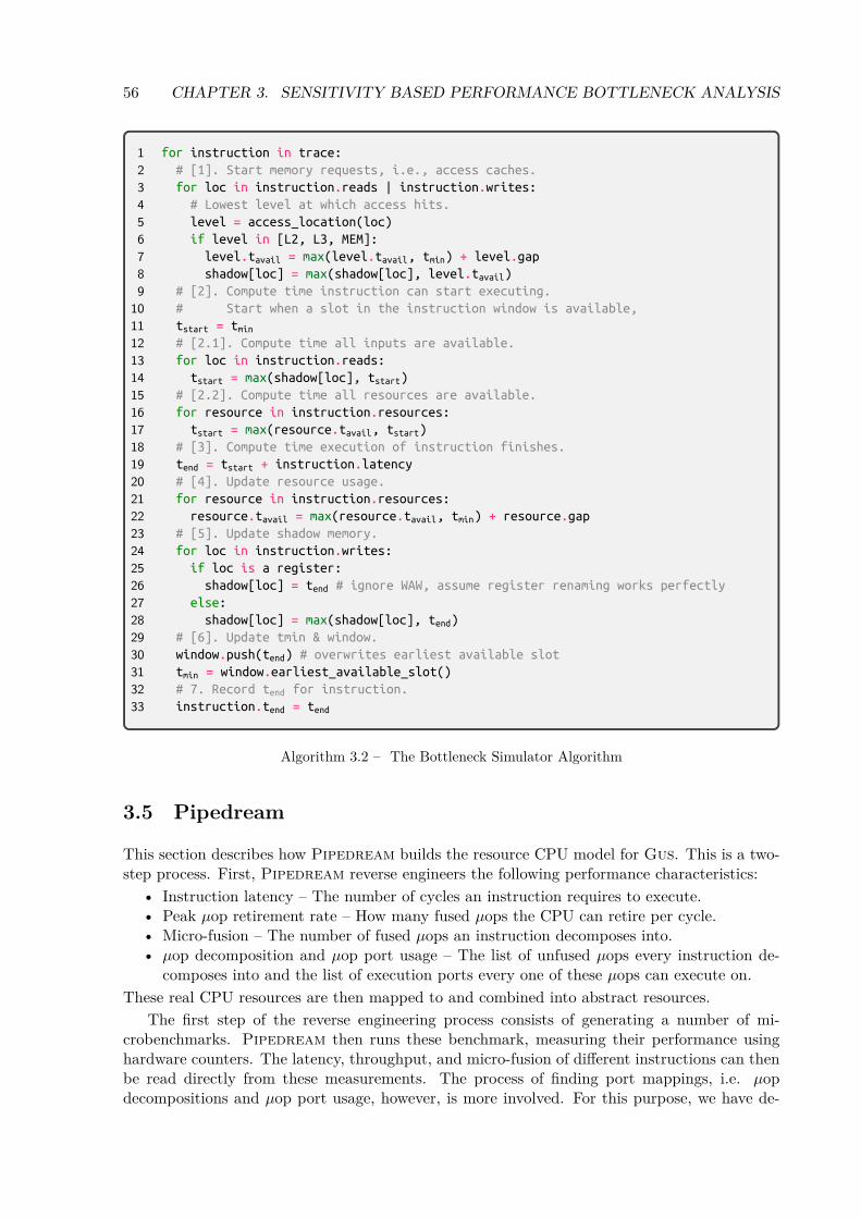
56 CHAPTER 3. SENSITIVITY BASED PERFORMANCE BOTTLENECK ANALYSIS
1 for instruction in trace:
2 # [1]. Start memory requests, i.e., access caches.
3 for loc in instruction.reads | instruction.writes:
4 # Lowest level at which access hits.
5 level = access_location(loc)
6 if level in [L2, L3, MEM]:
7 level.tavail = max(level.tavail, tmin) + level.gap
8 shadow[loc] = max(shadow[loc], level.tavail)
9 # [2]. Compute time instruction can start executing.
10 # Start when a slot in the instruction window is available,
11 tstart = tmin12 # [2.1]. Compute time all inputs are available.
13 for loc in instruction.reads:
14 tstart = max(shadow[loc], tstart)
15 # [2.2]. Compute time all resources are available.
16 for resource in instruction.resources:
17 tstart = max(resource.tavail, tstart)
18 # [3]. Compute time execution of instruction finishes.
19 tend = tstart + instruction.latency
20 # [4]. Update resource usage.
21 for resource in instruction.resources:
22 resource.tavail = max(resource.tavail, tmin) + resource.gap
23 # [5]. Update shadow memory.
24 for loc in instruction.writes:
25 if loc is a register:
26 shadow[loc] = tend # ignore WAW, assume register renaming works perfectly
27 else:
28 shadow[loc] = max(shadow[loc], tend)
29 # [6]. Update tmin & window.
30 window.push(tend) # overwrites earliest available slot
31 tmin = window.earliest_available_slot()
32 # 7. Record tend for instruction.
33 instruction.tend = tend
Algorithm 3.2 – The Bottleneck Simulator Algorithm
3.5 Pipedream
This section describes how Pipedream builds the resource CPU model for Gus. This is a two-step process. First, Pipedream reverse engineers the following performance characteristics:
• Instruction latency – The number of cycles an instruction requires to execute.• Peak µop retirement rate – How many fused µops the CPU can retire per cycle.• Micro-fusion – The number of fused µops an instruction decomposes into.• µop decomposition and µop port usage – The list of unfused µops every instruction de-
composes into and the list of execution ports every one of these µops can execute on.These real CPU resources are then mapped to and combined into abstract resources.
The first step of the reverse engineering process consists of generating a number of mi-crobenchmarks. Pipedream then runs these benchmark, measuring their performance usinghardware counters. The latency, throughput, and micro-fusion of different instructions can thenbe read directly from these measurements. The process of finding port mappings, i.e. µopdecompositions and µop port usage, however, is more involved. For this purpose, we have de-

3.5. PIPEDREAM 57
fined a variation of the maximum flow problem which we call the instruction flow problem. Wehave developed a linear program (LP) formulation of the instruction flow problem which can beused to calculate the peak IPC and micro-operations per cycle (MPC) a benchmark kernel cantheoretically achieve with a given port mapping. The actual port mapping of the underlyinghardware is then determined by finding the mapping for which the throughput predicted byinstruction flow best matches the actual measured IPC and MPC.
The counters required by Pipedream for its measurements the are:• An accurate cycle counter, to calculate the IPC.• A counter for the total number of retired µops, to calculate the fused MPC.• A counter for the total number of µops executed on any execution port, to calculate the
unfused MPC.• A counter for each execution port that counts the number of unfused µops executed on
that port.All of these counters are available on Intel CPUs since Sandy Bridge. For now, we have built amodel of the Skylake architecture.
The CPU model used in instruction flow is even simpler than that of Gus. It only considersinstructions, µops, and the throughput of execution ports. Any other components, such asthe ROB, the instruction scheduler, or latencies, are not directly taken into account. Thebenchmarks we apply the model to are all constructed in a way so that these resources neverform a bottleneck.
In the following we will use [i1i2 . . . in] to denote a microkernel consisting of n instructionsi1 through in. By construction our kernels never have any data dependencies, so the order ofinstructions in a kernel is not relevant. That is, [i1i2] = [i2i1]. The number of occurences ofan instruction in a kernel, however, is relevant. Thus, [i1i1i2] 6= [i1i2]. We the plus symbol todenote the concatenation of kernels, i.e. [i1] + [i2] = [i1i2]. We also use the shorthand AN todenote N repetitions of instruction A. So, for example, [i21i32] = [i1i1i2i2i2].
Throughout the rest of this chapter we use a variation of Agner Fog’s notation for executionports, µops, and µop decomposition [72]. Execution ports are noted as p0 . . . pn. The identifierfor a µop is simply the concatenated sequence of ports it can execute on. That is, a µop thatcan execute only on port p4 will be written as p4. A µop that can execute on either p1 or p3 isdenoted as p13. For simplicity, we will assume that there are at most ten execution ports so thatthey can be labelled with a single digit. A µop decomposition is simply the list of identifiers forevery µop. If a µop occurs multiple times in a decomposition, it is prefixed with the number ofoccurrences. An instruction that decomposes into three µops, two of type p015 and one of typep6, is written as 2p015 p6.
3.5.1 The instruction flow problem
Before describing the algorithm for finding port mappings, we introduce the instruction flowproblem. The instruction flow problem is a variation of the maximum flow problem whichallows for constraints that force the total flow that passes through two nodes to be equal. Weuse the instruction flow to model the steady state of a CPU with a given port mapping when itis executing a small microkernel in an infinite loop. The “flow” through such an instruction flowproblem models the rates at which instructions and µops execute on the execution ports of theCPU. That is, a solution for an instance of the instruction flow problem directly encodes theIPC, MPC and execution port usage a kernel can achieve. Solving instruction flow instances isthe core mechanism used in Pipedream to evaluate and find port mappings.
Pipedream uses the same notion of µop as Gus. That is, a µop is simply a list of executionports, and we do not consider the latency of µops nor data dependencies between them.
We define an instance of the instruction flow is a multipartite directed acyclic graph (DAG)

58 CHAPTER 3. SENSITIVITY BASED PERFORMANCE BOTTLENECK ANALYSIS
G = (V,E), where V = ({kIPC} ∪· I ∪· M ∪· P ∪· {kMPC}) is a set of vertices and E ⊆ V × V is aset of edges. V is partitioned into several disjoint subsets:
• {kIPC} – This singleton set contains the source vertex kIPC through which flow entersthe system. Conceptually, it is this vertex from which instructions flow into the CPU toexecute, and so the flow entering at this point is the total IPC for the kernel.
• I – The set of vertices I represents the different instructions in the kernel. There is onlyone instruction vertex per type of instruction. I.e., if a kernel contains two add instructionsthere will be only one iadd ∈ I vertex to model this.
• M – The set of vertices M represents the different µops that instructions decompose to.Some instructions can decompose into more than one µop of a given type, but for simplicity,we do not model this directly. Instead, if an instruction i decomposes into n instances ofµop m there will be n distinct vertices m1, . . . ,mn.
• P – The set of vertices P represents the different execution ports of the modelled CPU.• {kMPC} – This singleton set contains the sink vertex kMPC through which flow leaves the
system. Conceptually, it is this vertex at which µops execute and leave the CPU, so theflow leaving through this vertex is the total MPC for the kernel.
No two vertices inside one of the partitions in V can be connected by an edge, and there areonly edges between partitions. Only edges between the following pairs of partitions are allowed:
• From {kIPC} to I – These edges indicate which instructions the kernel contains. Everyinstruction is connected to kIPC .
• From I to M – These edges give the decomposition of instructions into µops.• From M to P – These edges describe which execution port a µop can execute on.• From P to {kMPC} – These are the edges through flow leaves the system. Every port is
Every port is connected to kMPC .We usually omit kIPC and kMPC when drawing instruction flow graphs.
µop and port vertices follow the standard rules for the conservation of flow in a flow network.That is, the sum of all flow entering such a vertex via its incoming edges equals the flow leavingit via its outgoing edges. This does, however, not hold for instruction vertices. When aninstruction decomposes into multiple µops it puts more pressure on the execution ports thanan instruction that only produces one µop, i.e. the MPC of the kernel will be larger than itsIPC. Consequently, when an instruction decomposes into more than one µop the flow leavingthe vertex representing it in the instruction flow graph is larger than the incoming flow. To beprecise, the total outgoing flow of an instruction vertex is equal to the incoming flow times thenumber of µops it decomposes into. On the other hand, when a µop is connected to more thanone port, this means that the µop can execute on either of these ports, but it only goes to oneof them. So at this level conservation of flow is upheld and the MPC is distributed along thedifferent outgoing edges.
Besides the graph G, an instruction flow instance of also encompasses a set of constants thatfurther describe the kernels and certain characteristics of the CPU architecture being modelled.
oi ∈ N0 – The number of times an instruction i ∈ I occurs in the kernel. If oi = 0 then(k, i) /∈ E. Likewise, if oi 6= 0 then (k, i) ∈ E.λmax ∈ R+ – The maximum fused MPC attainable on the CPU architecture. This issimply the maximum fused MPC observed during any benchmark run. This models theretirement bottleneck of the ROB. We need to take this into account since Intel CPUs cantheoretically execute more µops than they can retire.#λi ∈ N – The number of fused µops an instruction i ∈ I decomposes to.#µi ∈ N – The number of unfused µops an instruction i ∈ I decomposes to. Thiscorresponds to the number of outgoing edges of the the i vertex.
A solution of an instance of the instruction flow assigns a weight to every vertex and edge inG. These weights correspond to IPC or MPC that passes through that part of the graph. We

3.5. PIPEDREAM 59
kIPC
i1 i2
m1 m2 m3
p1 p2 p3 p4
kMPC
ρk, λk
oi1 oi2
ρi1 ,λi1 ,µi1 ρi2 ,λi2 ,µi2
λi1,m1λi1,m2 λi2,m3
µi1,m1 µi1,m2µi2,m3
λm1 ,µm1 λm2 ,µm2 λm3 ,µm3
µm1,p1 µm1,p2 µm2,p3 µm3,p3 µm3,p4
µp1 µp2 µp3 µp4
µk
Kernel
Instructions
Muops
Ports
Total IPC and fused MPC for kernel
Number of occurences of instr. in kernel
Total IPC, fused MPC, and unfusedMPC for all instances of instr. in kernelFused MPC between instruction and µop
Unfused MPC between instruction and µop
Total fused and unfused MPC of µop
Unfused MPC between µop and port
Total unfused MPC of port
Total unfused MPC for kernel
Figure 3.3 – Example instance of the instruction flow problem. An instance of an instruction producesone µop for every outgoing edge, i.e., i1 decomposes into one m1 and one m2. One instance of a µop onlyexecutes on one port, i.e., m1 can execute either on p1 or p2.
use the following notation for the weights of the different types of vertices and edges:• ρk – The total IPC of kernel.• λk – The total fused MPC of kernel.• ρi – The IPC for all instances of instruction i in the kernel. The same instruction can
have different IPCs in different kernels due to differing execution port usage.• λi – The total fused MPC of all µops generated for all instances of instruction i in the
kernel.• µi – The total unfused MPC of all µops generated for all instances of instruction i in the
kernel.• λi,m – The fused MPC of µop m generated from all instance of instruction i in the kernel.• µi,m – The unfused MPC of µop m generated from all instance of instruction i in the
kernel.• λm – The total fused MPC of all µops generated for all instructions in the kernel.• µm – The total unfused MPC of all µops generated for all instructions in the kernel.• µm,p – The unfused MPC of µop m executed on port p in the kernel.• µp – The total unfused MPC of all µops executed on port p in the kernel.• µk – The total unfused MPC of kernel.
An example instance of the instruction flow problem indicating which weight is on which nodeor edge can be seen in Figure 3.3
A valid solution for an instance of the instruction flow problem must maximize the total flowgiven the following constraints:C1 – ρk =
∑i∈I ρi

60 CHAPTER 3. SENSITIVITY BASED PERFORMANCE BOTTLENECK ANALYSIS
C2 – λk =∑
i∈I λi
C3 – µk =∑
p∈P µp
(total flow in and out of system)
C4 – ∀i ∈ I. µi =∑
m∈M µi,m
C5 – ∀m ∈ M. µm =∑
i∈I µi,m
C6 – ∀m ∈ M. µm =∑
p∈P µm,p
C7 – ∀p ∈ P. µp =∑
m∈M µm,p
(conservation of flow)
C8 – ∀i ∈ I. (kIPC , i) /∈ E =⇒ ρi = 0C9 – ∀i ∈ I,m ∈ M. (i,m) /∈ E =⇒ µi,m = 0C10 – ∀m ∈ M,p ∈ P. (m, p) /∈ E =⇒ µm,p = 0
(flow only propagates along edges)
C11 – ∀i1, i2 ∈ I. (oi2 > 0 ∧ oi2 > 0) =⇒ oi2 ∗ ρi1 = oi1 ∗ ρi2(IPC of kernel is split evenly among instructions)
C12 – ∀i ∈ I,m ∈ M. (i,m) ∈ E =⇒ ρi = µi,m
(unfused MPC is split evenly among µops for an instruction)
C13 – ∀i ∈ I. ρi =1
#µi∗∑
m∈M µi,m (translate IPC to unfused MPC)C14 – ∀i ∈ I. λi =
#λi
#µi∗ µi (translate fused MPC to unfused MPC)
C15 – ∀p ∈ P. µp ≤ 1 (a port executes at most one µop per cycle)C16 – λk ≤ λmax (µop retirement limit)C17 – ∀i ∈ I. µi ≤ µ[i] (bottlenecks other than retirement or ports)Figure 3.4 shows some instruction flow instances, each annotated with its solution according tothese constraints.
Constraints C1 – C10 encode the basic flow properties, like “the sum of flow entering a vertexequals the sum of flow leaving it” and “flow can only propagate along edges”. Remember thatinstruction vertices do not follow the standard rules for the conservation of flow. Constraint C13
models how flow entering these nodes is multiplied before leaving due to µop decomposition.By themselves, these constraints can easily be rewritten to a standard flow network for whicha maximal solution corresponds exactly to the maximum flow solution. Such a solution would,however, allow nonsensical behaviour, such as two different instructions in a kernel steadilyexecuting at different rates.
To forbid these solutions we add constraints C11 and C12. C11 forces the IPC to be spreadevenly among all instructions in a kernel, proportionally to the number of times they occur.Likewise, C12 forces all µops generated by an instruction to have the same MPC.
Constraints C15 and C16 limit the overall flow in the system by putting a bound on the rateat which µops can execute and retire. C15 encodes the maximum dispatch rate of executionports of one unfused µop per cycle and C16 encodes the maximum rate at which fused µops canbe retired. Note that C16 assumes all functional units of a CPU to be perfectly pipelined.
Finally, C17 limits the total MPC all µops for an instruction i can achieve by the total MPCof the kernel [i] containing only that instruction. For most instructions this will not imposeany additional throughput limitation not already encoded in C15 and C16. It does, however, tosome degree, allow handling instructions that are bottlenecked by CPU resources not currentlypresent in the model. An example of this is the add-with-carry (adc) or subtract-with-borrow(sbb) instructions on x86 which have an implicit data dependency via the flags register limitingtheir IPC. As stated earlier, the instruction flow problem generally assumes that there are no

3.5. PIPEDREAM 61
k = [i1] ρk = 2
i1
m1
p1 p2µp1 = 1 µp2 = 1
µk = 2
µi1,m1 = 2
µm1,p1 = 1 µm1,p2 = 1
(a) All ports fully utilized
k = [i1i2] ρk = 2
i1 i2
m1
p1 p21 1
µk = 2
1 1
1 1
(b) All ports fully utilized
k = [i1] ρk = 1
i1
m1 m2 m3
p1 p2 p31 1 1
µk = 3
1 1 1
1⁄2 1⁄21⁄2 1⁄2 1
(c) All ports fully utilizedk = [i1i2] ρk = 2
i1 i2
m1 m2
p1 p2 p31/2 1/2 1
µk = 2
1 1
1/2 1/2 1
(d) Throughput of kernel is limited by p3 andso p1 and p2 are not fully utilized.
k = [i1i2] ρk = 1
i1 i2
m1 m2 m3
p1 p21 1/2
µk = 11/2
1/2 1/2 1/2
1/2 1/2 1/2
(e) Throughput of kernel is limited by p1 andso p2 is not fully utilized.
Figure 3.4 – Example solutions to some simple instruction flow problems. For simplicity every instructiononly appears once in every kernel and no µop fusion occurs. The names of weights are only shown in a,in all other figures we only give the values of weights.
data dependencies. However, by adding C17 the IPC predicted for kernels containing these typesof instructions is still accurate enough to find exact port mappings. Examples of this will begiven in the experiments in Section 3.6.2.
Since in an instance of instruction flow G, oi, #µi, #λi, λmax, and µ[i] are fixed all the aboveconstraints are linear. They can thus be directly encoded as a linear optimization problemthat computes the IPC and MPC of every kernel on the given port mapping. The objectivefunction for this optimization problem is simply: maximizeµk That is, we maximize the weightsrepresenting the utilization of the execution ports in every kernel. Due to constraints C4 to C7
this “pressure” automatically propagates through the whole graph which determines the rest ofthe weights.
3.5.2 Finding port mappings
Now that we have introduced the instruction flow problem, we can show how it is used byPipedream to find a port mapping for a CPU architecture. The port mappings we producecorrespond the I, M , and P vertices from instruction flow and the edges between them. Thatis, for every instruction we find which µops it decomposes into and for every µop we find theports it can execute on.
The I level, that is, the instruction set of a CPU is usually well documented by vendors.For x86 we have used the ISA description from Intel xed. The P level, the execution ports,

62 CHAPTER 3. SENSITIVITY BASED PERFORMANCE BOTTLENECK ANALYSIS
k = [i1] ρk = 1/2
i1
m1 m2 m3
p2p1 1 1/2
µk = 11/2
1/2 1/2 1/2
1/2 1/2 1/2
k = [i1] ρk = 1/2
i1
m1 m2 m3
p1 p21/2 1
µk = 11/2
1/2 1/2 1/2
1/2 1/2 1/2
(a) Two port mappings with identical IPC andMPC, but differing port utilization
k = [i1] ρk = 2
i1
m1 m2
p1 p21 1
µk = 2
1 1
1 1
k = [i1] ρk = 2
i1
m1 m2
p1 p21 1
µk = 2
1 1
1/2 1/21/2 1/2
(b) Two port mappings with identical IPC andMPC, and port utilization
Figure 3.5 – Examples of port mappings that produce the same IPC and MPC
are also relatively well documented. Most vendors at least disclose the number of executionports an architecture has. However, which different µops a machine uses, what µops eachinstruction decomposes into, or even just the number of µops into which instruction decomposeis undocumented.
It is the goal of Pipedream to find this missing middle level of µops and the edges thatconnect all of the levels. The model produced by Pipedream, however, does not necessarilyperfectly reflect the real mapping and semantics of µops on the underlying hardware. We onlyneed a model that accurately reflects the performance and resource sharing of instructions foruse in Gus.
The first step in the reverse engineering process of Pipedream is to determine for everyinstruction i the number of fused and unfused µops it decomposes into and the execution portsthat it uses. In other words, we measure #λi, #µi and µp. This can be done directly using hard-ware performance counters and a single benchmark kernel [i]. To differentiate the empiricallymeasured values for µp from those calculated by instruction flow we note them as µemp,p. Forinstructions that decompose into a single µop, i.e., #µi = 1, this is already enough informationto find its µop decomposition. Since such an instruction has only one µop all ports p whereµemp,p 6= 0 must be used by that µop.
For instructions that decompose into more than one µop the situation is not as simple though,since the sets of ports used by different µops can overlap. For these types of instructions wesolve the instruction flow LP for each possible µop decomposition. We then compare this againstthe empirically measured total µop throughput, µemp,k. The decomposition of an instruction isthen assumed to be the one whose predicted throughput best matches the measured throughput,that is the mapping that minimizes the simulation error : |µk−µemp,k|
µemp,k2. There are, however, two
problems with this naïve algorithm.
Problem 1: There are usually a large number of different port mappings that produce thesame IPC, MPC and port usage. Figure 3.5 shows examples of such problematic cases.
Problem 2: Even though we do not have to enumerate all possible instruction flow instancesfor every instruction we still have to enumerate all possible µop decompositions. That is, the
2We could equally well define the simulation error using the predicted and measured IPC, ρk and ρemp,k, sincethe IPC and MPC are directly related.

3.5. PIPEDREAM 63
kIPC , I, M , and P nodes and the edges between kIPC , I, and M are fixed, but we need toenumerate all possible combinations of edges between the M and P nodes.
Solution for problem 1
k = [i1] ρk = 1
i1
m1 m2
p1 p21 1
µk = 2
1 1
1 1
k = [i1] ρk = 1
i1
m1 m2
p1 p21 1
µk = 2
1 1
1/2 1/21/2 1/2
(a) The two port mappings from Fig-ure 3.5b with identical IPC and MPC, andport utilization
k = [i1i2] ρk = 1
i1 i2
m1 m2 m3
p1 p21/2 1
µk = 11/2
1/2 1/2 1/2
1/2 1/2 1/2
k = [i1i2] ρk = 11/3
i1 i2
m1 m2 m3
p1 p21 1
µk = 2
2/3 2/3 2/3
1/2 1/61/2 1/6 2/3
(b) By adding i2 to the kernel we can distinguish thetwo port mappings
Figure 3.6 – Example of how additional instructions can be used to distinguish port mappings
If we look at the two-port mappings shown in Figure 3.5a, we see that while they producethe same IPC and MPC the utilization of individual ports differs. We can extend the instructionflow LP to be able to distinguish these kinds of mappings by adding the following constraints:C18 – ∀p ∈ P. µemp,p − err ≤ µp ≤ µemp,p + err
(valid range for port utilization)C19 – ∀p ∈ P. 0 ≤ errµ,p ≤ maxerr
(upper bound for err, maxerr is a constant)Constraint C18 simply enforces that the usage of individual ports in an instruction flow solutiondoes not differ too much from the actual measured usage. Here we do not fix the predicted µp
to exact values, but only force them to be within an error margin err of the measured values.We do this since, in practice, performance counters are not perfectly accurate, and there is somenoise in the measurements. The LP solver often cannot find any valid solution for any portmapping if we fix exact values for the port usage. For the LP we now use two optimizationsobjectives: First, minimizeerr, and second, as before, maximizeµk. That is, we first find theminimum value for err for which there is a solution, and we then find a solution that maximizesthe throughput. Any solution for the second objective may not have a higher err than thatfound by the first objective. This type of lexicographic optimization problem with multipleobjectives is directly supported by gurobi, the LP solver we use. Finally, constraint C19 setsan upper bound for the maximum value of err. In practice, we set maxerr to a small enoughvalue so that the LP solver still finds a solution, for most instructions this is 0.1.
In practice, setting bounds on the port usage helps to speed up the LP solver. Usually, thereare many mappings for which the solver can very quickly determine that there is no solutionthat can reproduce the observed throughputs. In our experience, the LP solver can filter outsuch infeasible mappings in under ten milliseconds while calculating a feasible solution can takeseveral 100 milliseconds.
There are, however, port mappings that still can not be distinguished with this method. Anexample of this is shown in Figure 3.5b. We use the same general approach as Agner Fog [72] anduops.info [3] to find port mappings for these instructions. That is, to find the decomposition

64 CHAPTER 3. SENSITIVITY BASED PERFORMANCE BOTTLENECK ANALYSIS
for an instruction i, we generate multiple kernels that mix i with other instructions with aknown decomposition and measure how they interact. An example of how this works can beseen in Figure 3.6. Algorithm 3.3 shows how Pipedream uses this technique to find the µopdecomposition is multi-µop instructions. Using single-µop instructions, whose decomposition wecan easily find, we generate benchmarks that individually block all ports used by i.
Ideally, the single-µop instruction in every kernel would use exactly one port, however notevery architecture has such an instruction for every port. On x86 processors, for example, thereare two identical ports to handle the data transfer for memory reads. Any load µop can executeon either one of these two ports. Consequently, we generate one benchmark kernel for every µopthat can be generated by a single-µop instruction. The number of different such µops is relativelysmall since we do not consider the semantics of µops, but only the ports they use. On x86, forexample, integer addition, subtraction, any bitwise logical operations, and compare instructionsall produce the same µop, i.e. use the same ports, even though they perform a variety of differenttasks. The final µop decomposition for an instruction is then the one that minimizes the averagesimulation error 1
k
∑ |µk−µemp,k|µemp,k
for all k kernels. If there are multiple decompositions with thesame simulation error we choose the one with the least number of edges between M and P .Section 3.6.2 will further explain this reasoning.
Solution for problem 2
A naive implementation of our algorithm for finding µop decompositions has to enumerate allpossible decompositions for every different instruction, which is equivalent to enumerating allbipartite graphs. For an instruction with m µops on a CPU with p ports there are approximately∑p
k=1
(pk
)(−1)p−k(2k−1)m such graphs [87]. Let us illustrate how many different decompositions
there are in practice with a small example. On any Intel Haswell, Broadwell, or Skylake x86CPU has eight execution ports, and the median number of µops an instruction decomposesinto is two. Given these points, there are 183700 different possible µop decompositions for anaverage instruction. These are, of course, far too many graphs to test in a reasonable time since
for i in MULTI_MUOP_INSTRUCTIONS():
measurements = MEASURE_KERNEL_PERFORMANCE([i])
for muop in MUOPS_GENERATED_BY_SINGLE_MUOP_INSTRUCTION():
if PORTS_USED(i) != PORTS_USED(muop):
continue
simple_inst = INSTRUCTION_GENERATING_MUOP(muop)
measurements += MEASURE_KERNEL_PERFORMANCE([simple_inst])measurements += MEASURE_KERNEL_PERFORMANCE([i simple_inst])
best_muop_decomposition = None
smallest_error = ∞
for muop_decomposition in POSSIBLE_MUOP_DECOMPOSITIONS():
simulation_error = SOLVE_INSTFLOW_LP(muop_decomposition, measurements)
if simulation_error < smallest_error:
best_muop_decomposition = muop_decomposition
smallest_error = simulation_error
Algorithm 3.3 – Algorithm to find µop decomposition with per execution port hardware counters

3.5. PIPEDREAM 65
we have to solve an LP problem for every such graph. To reduce the number of different µopdecompositions we have to evaluate for an instruction i we use two techniques:
1. We only consider decompositions using the same ports as i. As stated above, all recent IntelCPU architectures have eight execution ports. However, the average instruction only usesfour of these ports. Therefore, for an average instruction, we only need to consider around80 different µop decompositions. Nevertheless, the number of possible decompositions stillgrows very rapidly, and, in practice, this approach can only handle instructions with upto three µops using up to four ports.
2. We can optionally also assume that all µops of an architecture can be produced by asingle-µop instruction [3]. This way we no longer have to enumerate all possible bipartitegraphs, but only all words over the alphabet of µops. For an instruction with m µops ona CPU with N different µops there are then mN possible decompositions. On Skylake, forexample, there are roughly 15 different µops. At first glance, this does not seem like animprovement over the previous technique, since we now have to explore 215 ≈ 32thousanddifferent decompositions for the average instruction. However, we do not always have toconsider all 15 µops for every instruction. We only need to try µops that use a subset ofthe overall set of ports used by an instruction.In practice, this very significantly reduces the number of possible decompositions for aninstruction. On Intel architectures the common case of an instruction that decomposesinto a computation µop and a memory load µop there is only ever one possible mappingsince the ports responsible for load/store and computations are distinct. Even instruc-tions that decompose into four or five µops usually have less than one hundred possibledecompositions.However, this assumption that all µops of an architecture can be generated using onlysingle-µop instructions actually does not hold on x86. The one exception to this arememory store operations, which always decompose into at least two µops. However, bothof these µops use a dedicated execution port, port 4 and port 7 respectively, which meanswe can easily detect instructions which use “impossible” µops Pipedream does not knowabout yet. In these cases, Pipedream falls back to the first technique to find these newµops. Once it has added the new µop to its list, other store instructions can be handledmuch faster.
3.5.3 Converting port mappings to resource models
Once Pipedream has constructed a port mapping, we can convert it to a resource mappingas used by Gus as described in Section 3.4.3. In this model, we create the following abstractresources:
• Execution ports – We create one resource per execution port of the CPU. Since a portcan accept one instruction per cycle, the throughput of each of these resources is one. Tomodel µops that can execute on multiple execution ports, we also create virtual resourcesrepresenting the combinations ports. By default, the throughput of combined resources isequal to the sum of the throughputs of all sub-resources from it is composed.
• µop retirement – We create one global resource to represent fused µop retirement limitwhose throughput is equal to the measured λmax. Every instruction uses this resourceproportionally to the number of fused µops it produces.
• Instruction throttles – Some instructions have a throughput that is limited by other CPUresources than functional units or the ROB. This behaviour is detected by Pipedream byobserving that the peak throughput of an instruction is significantly lower than its portmapping allows. For every such instruction i we create an abstract resource with the samethroughput as the kernel [i].

66 CHAPTER 3. SENSITIVITY BASED PERFORMANCE BOTTLENECK ANALYSIS
1. spill registers to stack
2. flush CPU pipeline
3. start PAPI performance counters
4. spill PAPI handles to stack
5. flush CPU pipeline
6. initialize values in registers (optional)
7. benchmark-loop
8. flush CPU pipeline
9. restore PAPI handles from stack
10. read PAPI performance counters
11. flush CPU pipeline
12. restore registers
Figure 3.7 – General design of benchmarks generated by Pipedream
3.5.4 Benchmark design
To take the required measurements for building Gus’s CPU model Pipedream uses automat-ically generated microbenchmarks written x86 assembler. All benchmarks are generated froma ISA description extracted from Intel xed [55]. Every benchmark is one procedure written intextual assembler, which is then assembled using GNU gas. Multiple benchmarks are packagedinto one shared library and then loaded into the Pipedream process for execution.
Pipedream benchmarks run in user-space and do not require root privileges on a machine.As a consequence we can not directly read hardware performance counters with the rdpmc in-structions since it is by default only accessible from ring 0, i.e. kernel space. Instead, we have touse a system call to read counters. For convenience and portability, we use PAPI [65] for this.Using a system call to read performance counters has some wide-reaching consequences we haveto account for in our benchmark design.
In general, the microbenchmark kernels we are interested in are tiny, consisting only of ahandful of instructions, usually between one and five. However, the overhead of reading perfor-mance counters is much too high to such tiny kernels with any reasonable degree of accuracy.As a consequence, we have to repeatedly execute a kernel many times. Nevertheless, simplyunrolling the kernel thousands of times may introduce skew the results of the measurements byputting stress on the instruction decoder or instruction cache. To avoid this skew, we insteadwrap the kernel in a simple, statically counted loop. Since the instructions used to implementthe loop also use some CPU resources which distorts the measurements we do unroll the kernelseveral times. The unrolling factor is chosen so that the loop still fits in the µop cache. Sincemodern CPUs have large µop caches with upwards of a thousand entries, the benchmark loopcan safely be unrolled several dozen of times.
Figure 3.7 shows the general design of all benchmarks generated by Pipedream. The CPUpipeline flushes in steps 2. and 5., implemented using a serializing instruction, prevent theCPU from reordering instructions from before the kernel to execute after performance countershave been started. Likewise, the flushes in steps 8. and 11. prevent instructions from inside thekernel to be executed after the counters have been read. Inside the benchmark kernel, we reserveone general-purpose register for the loop counter and, if the benchmark contains load/storeinstructions, another register as a base register for memory accesses. All other registers areavailable to the benchmark kernel. Register allocation in benchmarks is done after unrolling thekernel to prevent any unwanted false dependencies. We also allocate a large contiguous block

3.5. PIPEDREAM 67
.kernel.loop.head:
# vaddps SRC1, SRC2, DST
vaddps %ymm1, %ymm1, %ymm0
vaddps %ymm1, %ymm1, %ymm2
vaddps %ymm1, %ymm1, %ymm3
vaddps %ymm1, %ymm1, %ymm4
...
# Decrement loop counter & iterate
# On Intel & AMD processors this is macro-fused into a single μop
sub $1, %r15
jne .kernel.loop.head
Figure 3.8 – Example benchmark to measure instruction throughput
.kernel.loop.head:
# vaddps SRC1, SRC2, DST
vaddps %ymm0, %ymm0, %ymm0
vaddps %ymm0, %ymm0, %ymm0
vaddps %ymm0, %ymm0, %ymm0
vaddps %ymm0, %ymm0, %ymm0
...
# Decrement loop counter & iterate
# On Intel & AMD processors this is macro-fused into a single μop
sub $1, %r15
jne .kernel.loop.head
Figure 3.9 – Example benchmark to measure instruction latency.
of memory called the memory arena. All load and store instructions are assigned a constantaddress inside this arena.
Pipedream can also initialize any registers to a fixed value before the kernel executes, asshown in step 6.. Usually, all registers are initialized to zero, but some instructions requiredregisters to be initialized to some special value. Integer division, for example, raises an exceptionif the divisor is zero, so we appropriately initialize registers to avoid this.
Pipedream can not yet generate benchmarks for instructions that use a rep prefix, a lock
prefix, or AVX512 instructions. In total, it can generate benchmarks for just over 2800 differentinstructions.
As cycle counter we used CPU_CLK_UNHALTED. To count the total number of µops executedin a benchmark we used the counters UOPS_RETIRED:ALL, for unfused µops, and UOPS_RETIRED-
:RETIRE_SLOTS for fused µops. To count the number of µops executed on each execution portwe used UOPS_EXECUTED_PORT:PORT_0/1/. . . /7. Finally, we used the average value over all runsfor each counter.
Measuring instruction throughput and port usage
To measure the throughput of an instruction, i.e., how many instances of that instruction aprocessor can execute per cycle, we again generate a benchmark kernel containing only copies ofthat instruction. We then allocate the registers in the benchmark to create as many independentdependency chains as possible. To the same end, all load instructions are set to read from the
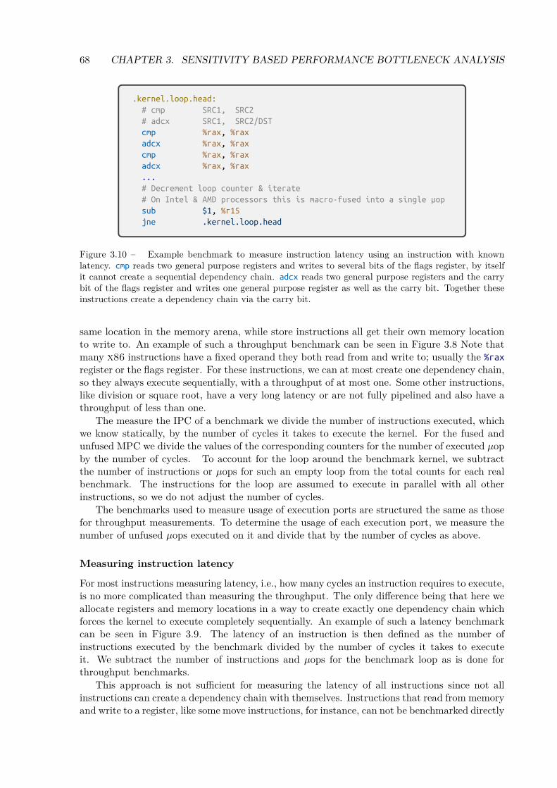
68 CHAPTER 3. SENSITIVITY BASED PERFORMANCE BOTTLENECK ANALYSIS
.kernel.loop.head:
# cmp SRC1, SRC2
# adcx SRC1, SRC2/DST
cmp %rax, %rax
adcx %rax, %rax
cmp %rax, %rax
adcx %rax, %rax
...
# Decrement loop counter & iterate
# On Intel & AMD processors this is macro-fused into a single μop
sub $1, %r15
jne .kernel.loop.head
Figure 3.10 – Example benchmark to measure instruction latency using an instruction with knownlatency. cmp reads two general purpose registers and writes to several bits of the flags register, by itselfit cannot create a sequential dependency chain. adcx reads two general purpose registers and the carrybit of the flags register and writes one general purpose register as well as the carry bit. Together theseinstructions create a dependency chain via the carry bit.
same location in the memory arena, while store instructions all get their own memory locationto write to. An example of such a throughput benchmark can be seen in Figure 3.8 Note thatmany x86 instructions have a fixed operand they both read from and write to; usually the %rax
register or the flags register. For these instructions, we can at most create one dependency chain,so they always execute sequentially, with a throughput of at most one. Some other instructions,like division or square root, have a very long latency or are not fully pipelined and also have athroughput of less than one.
The measure the IPC of a benchmark we divide the number of instructions executed, whichwe know statically, by the number of cycles it takes to execute the kernel. For the fused andunfused MPC we divide the values of the corresponding counters for the number of executed µopby the number of cycles. To account for the loop around the benchmark kernel, we subtractthe number of instructions or µops for such an empty loop from the total counts for each realbenchmark. The instructions for the loop are assumed to execute in parallel with all otherinstructions, so we do not adjust the number of cycles.
The benchmarks used to measure usage of execution ports are structured the same as thosefor throughput measurements. To determine the usage of each execution port, we measure thenumber of unfused µops executed on it and divide that by the number of cycles as above.
Measuring instruction latency
For most instructions measuring latency, i.e., how many cycles an instruction requires to execute,is no more complicated than measuring the throughput. The only difference being that here weallocate registers and memory locations in a way to create exactly one dependency chain whichforces the kernel to execute completely sequentially. An example of such a latency benchmarkcan be seen in Figure 3.9. The latency of an instruction is then defined as the number ofinstructions executed by the benchmark divided by the number of cycles it takes to executeit. We subtract the number of instructions and µops for the benchmark loop as is done forthroughput benchmarks.
This approach is not sufficient for measuring the latency of all instructions since not allinstructions can create a dependency chain with themselves. Instructions that read from memoryand write to a register, like some move instructions, for instance, can not be benchmarked directly
3.6. EXPERIMENTS 69
with this approach. To measure the latency of these more complicated instructions, we add asecond instruction with an already known latency to the benchmark kernel so in order to createa sequential dependency chain. The latency of the first instruction is then determined as thelatency of the whole kernel minus the latency of the known instruction. For a small number ofinstruction types, less than 70, we even require two instructions with a known latency to createa dependency chain. Figure 3.10 shows a benchmark kernel containing two instructions tomeasure latency. Finally, there are some exotic instructions for controlling processor state thatdo not directly write to any registers or memory. Though Pipedream can create throughputbenchmarks for these instructions, it current has no way to reliably benchmark their latency.
Measuring micro-fusion
The benchmarks used to measure µop micro-fusion are simpler than those for throughput andlatency since they do not depend on timings. Here, we do not need to worry about decoding,and instruction or µop cache misses or data dependencies. So a benchmark can simply be along repeated sequence of the same instruction for which we measure the number of fused andunfused µops executed.
3.6 Experiments
Both Gus and Pipedream are still early prototypes under active development. This sectionhighlights preliminary results of their usefulness along several case studies.
3.6.1 Gus
3.6.1.1 Case study I: Matrix multiplication
The first case study shows how we optimize a matrix multiplication kernel based on feedback fromGus. Here we present a single-threaded version of the basic matrix-matrix product C := AB.All versions of the code are compiled with GCC 9.1 with the flags -O2. 3 All measurements aretaken on a Skylake 7940X running at 2.3 GHz using PAPI [65]. All reported measurements arethe median over ten executions.
We use square 192 × 192 matrices of 32 bit floating-point numbers. So each matrix uses144 kB of memory. Skylake CPUs have a 32 kB L1 cache and a 1MB L2 cache. Hence wecannot fit one whole matrix in L1, but all three matrices can fit in L2.
The resource mappings used for the simulator have been produced with Pipedream. Forinstructions that Pipedream cannot benchmark yet, such as conditional branches, we use themappings of Agner Fog [72]. The data-transfer bandwidth between individual cache levels andmemory have been determined using simple microbenchmarks.
For the sensitivity analysis we first run one simulation of a kernel with the default throughputfor all resources and default instruction latency. We then run one 15 simulations per resource,each time incrementing the throughput of that resource by 1%. We configure Gus to onlysimulate the performance of the computational kernel. The rest of the benchmark program,that is the code to initialize data structures and print results, are only simulated functionally.
Step I: Naive matrix multiplicationWe start from the basic naive implementation of a matrix multiplication, seen below. N is
set to 192.3All benchmarks here are limited to 128 bit SSE instructions, since QEMU does not support newer vector
instructions yet.

70 CHAPTER 3. SENSITIVITY BASED PERFORMANCE BOTTLENECK ANALYSIS
for (int i = 0; i < N; i++) {
for (int j = 0; j < N; j++) {
for (int k = 0; k < N; k++) {
C[i * N + j] += A[i * N + k] * B[k * N + j];
}}}
The naive matrix multiplication kernel has a runtime of approximately 25 million cycles onthe test machine. It takes 3.5 cycles to perform one accumulation into C, that is, to executeone iteration of the innermost loop. This corresponds to 0.5 32 bit floating-point operations percycle (FLOPs/cycle).
There are likely two performance bottlenecks in this code. The first is the fact that thematrix B is traversed with a stride of N along the innermost k loop. That is, while it is stored inrow-major order, the algorithm traverses it in column-major order. This is likely to cause a largenumber of cache misses depending on the value of N. The second possible problem is that theinnermost loop forms a reduction in C[i * N + j]. This reduction prevents any instruction-levelparallelism and forces the CPU to execute all iterations of the innermost sequentially.
Even for such a small example, it is not necessarily trivial to analytically detect which ofthe two problems forms the bigger bottleneck. Instead of manually analysing the kernel, weuse Gus’s sensitivity analysis. It finds that the performance is limited most by the bandwidthbetween the L1 and L2 cache. This is due to a large number of misses in the L1 cache whereeach miss causes data movement between L1 and L2. A visual representation of the results ofthe sensitivity analysis produced by our tool is shown below. We use a form of heat-map for thevisualization. Each bar in it represents one abstract resource. The height of each bar and itscolour indicate the speedup predicted by Gus if the throughput of that resource is increased.Take, for example, the resource L2 THR, which represents the throughput between L1 and L2.The graph shows that an increment of its throughput by 1% decreases the overall runtime ofthe kernel by 1%. If we increment the resource’s throughput by 2%, the runtime decreases byapproximately 2%. The bar fades to white around the 13 − 14% mark, which indicates that a15% increase in throughput produces a 13− 14% speedup. All other resources immediately faceto white at the 0% mark. That is, according to Gus, the runtime of the kernel is not affectedby increasing the throughput of any other resource. Hence, L2 THR is the bottleneck of thisversion of the kernel.
INST
LAT
L1THR
L2THR
L3THR
MEM
THR
L1SIZE
L2SIZE
L3SIZE
INST
RET P0 P1 P2 P3 P4 P5 P6 P7P0
1P06P15P16P23P46P015P237
P0156
15.014.013.012.011.010.09.08.07.06.05.04.03.02.01.00.0
Speedup(in%)
0
2
4
6
8
10
12
14
16
Resou
rceincrem
ent(in
%)

3.6. EXPERIMENTS 71
To improve the performance of the matrix multiplication kernel we need to apply a trans-formation that reduces its usage of the bandwidth between L1 and L2. In general, we considerthree different optimizations for such cases:
1. Loop interchange – Changing the order of loops in a loop nest can improve cache usageby changing the strides of memory accesses.
2. Loop tiling – Tiling splits the iteration space of a loop nest into smaller tiles to ensurethat data stays in cache until it is reused. Loop tiling is more difficult to apply since itintroduces new loops into the kernel, which increases the number of control instructions,such as branches and comparisons. Have more loops with a smaller trip count may alsonegatively affect branch prediction. It is also non-trivial to find optimal tile sizes to ensurethat data stays resident in the cache.
3. Data layout and alignment changes – Changing the alignment or layout of data can reduceconflict cache misses. In this case, we could pad the matrices with additional unusedelements to ensure that the ways of the cache are fully utilized. However, changing thealignment and layout of data is a non-local change that requires code outside the kernelfor allocating and inspecting the matrices to be modified too.
Here, we chose to perform a loop interchange on the kernel since it is the simplest of the threetransformations.
Step II: Loop interchangeWe perform a loop interchange that changes the order of loops from ijk to kij.
for (int k = 0; k < N; k++) {
for (int i = 0; i < N; i++) {
for (int j = 0; j < N; j++) {
C[i * N + j] += A[i * N + k] * B[k * N + j];
}}}
The loop interchange improves the runtime of the kernel from 25 million to 15 million cycles. Itnow takes 2.1 cycles to execute one iteration of the innermost loop, and the FLOPs/cycle risefrom 0.5 to 0.9. More detailed statistics are given in Table 3.1. There are two reasons why theinterchange increases the performance of the kernel:
• Changing the order of loops also changes the strides of the memory accesses to the differentmatrices. It notably causes the kernel to traverse the matrix B in row-major instead ofcolumn-major order.
• The innermost loop of the kernel now no longer forms a reduction in C[i * N + j], whichexposes a large amount of parallelism since all iterations of the innermost can now executein parallel.
Our sensitivity analysis now reports that the bottleneck of the modified kernel is now no longerthe bandwidth between L1 and L2 but the rate at which the ROB can retire µops. In thevisualization below, this is represented by the resource INST RET, which is used by everyinstruction. µop retirement is now a bottleneck due to the large amount of instruction levelparallelism exposed by the interchange.

72 CHAPTER 3. SENSITIVITY BASED PERFORMANCE BOTTLENECK ANALYSIS
INST
LAT
L1THR
L2THR
L3THR
MEM
THR
L1SIZE
L2SIZE
L3SIZE
INST
RET P0 P1 P2 P3 P4 P5 P6 P7P0
1P06P15P16P23P46P015P237
P0156
15.014.013.012.011.010.09.08.07.06.05.04.03.02.01.00.0
Speedup(in%)
0
2
4
6
8
10
12
14
16Reso
urce
increm
ent(in
%)
To further improve the performance of the matrix multiply kernel, we need to reduce thenumber of instructions that the CPU needs to retire per entry of the matrices. For kernels thatare bounded by the ROB we consider three different optimizations:
1. Vectorization – Most vector instructions use the same number of slots in the ROB as theirscalar counterparts. By replacing scalar instructions with vector instructions we can thuseffectively increase the number of computations performed per µop.
2. Loop unrolling – Unrolling loops reduces the number of control instructions and also oftenexposes other redundant computations that can be removed. It is also often required toenable vectorization.
3. Redundancy elimination – This general involves manually removing redundant computa-tions, such as factoring out terms in strided accesses, not already detected by the compiler.
In the current version of the code the compiler has already used the sophisticated addressingmodes available on x86 to fold address computation, loads, stores, and arithmetic operationsinto as few instructions as possible. There is no redundancy left remove. The kernel is, however,a perfect candidate for unrolling and consecutive vectorization.
Simulator Real execution
Kernel Cycles L1 misses L2 misses Cycles L1 misses L2 misses
Naive 25,688,364 7,224,804 6914 25,390,280 7,281,762 6076Loop interchange 12,451,163 481,539 6914 15,165,666 474,428 5682
Table 3.1 – Effects of a loop interchange on the matrix multiplication kernel
Step III: Loop unrolling and vectorizationTo reduce the µop retirement bottleneck in the interchanged kernel unroll the innermost j
loop and the vectorize the resulting code. We use 128-bit SSE vectors for this, which processfour 32 bit floating-point numbers at once. Consequently, we reduce the number of instructionsthat need to be retired per iteration of the innermost loop by approximately four. Anotheroptimization would to use a single fused multiply-add instruction (fma) instead of a seperatemultiply and add. However, QEMU currently does not support fma instructions on x86.

3.6. EXPERIMENTS 73
for (int k = 0; k < N; k++) {
for (int i = 0; i < N; i++) {
for (int j = 0; j < N; j += 4) {
// set all elements of vector a to A[ i * N + k]
__m128 a = _mm_set_ps1(A[ i * N + k]);
// vector load from C
__m128 c = _mm_load_ps(&C[i * N + j]);
// vector load from B
__m128 b = _mm_load_ps(&B[k * N + j]);
// c = (a * b) + c
c = _mm_add_ps(_mm_mul_ps(a, b), c);
// vector store to C
_mm_store_ps(&C[i * N + j], c);
}}}
This reduces the runtime of the kernel from 15 million cycles to 3.6 million cycles. It nowtakes 0.5 cycles instead of 2.1 to execute one accumulation into C. The FLOPs/cycle rise from0.9 to 3.9.
The sensitivity analysis for this version of the kernel finds that the µop-retirement bottleneckhas been removed. Instead, the bandwidth between L1 and L2 is again the main limiting factorfor performance.
INST
LAT
L1THR
L2THR
L3THR
MEM
THR
L1SIZE
L2SIZE
L3SIZE
INST
RET P0 P1 P2 P3 P4 P5 P6 P7P0
1P06P15P16P23P46P015P237
P0156
15.014.013.012.011.010.09.08.07.06.05.04.03.02.01.00.0
Speedup(in%)
0
2
4
6
8
10
12
14
16
Reso
urce
increm
ent(in
%)
We consider the same three optimizations as before for reducing the number of cache missesand reducing the of the bandwidth between L1 and L2: loop interchange, loop tiling, andchanges to the data alignment or layout. We have already performed a loop interchange, sothis is no longer an option. As before, we prefer to not require users to change their code andopt-out of changing the data alignment or layout. The remaining option is loop tiling.
Step IV: Loop tilingTo improve reuse of data in caches, we tile the i and j loops with a tile size of 32. The tiled
version no longer iterates over entire rows and columns of C directly. Instead, it operates on32× 32 sub-matrices that easily fit in the L1 cache. This optimization improves the runtime ofthe kernel from 3.6 million cycles to 3.2 million cycles. One accumulation into C now takes 0.45cycles to execute, and the FLOPs/cycle rise from 3.9 to 4.3.

74 CHAPTER 3. SENSITIVITY BASED PERFORMANCE BOTTLENECK ANALYSIS
for (int I = 0; I < N; I += 32) {
for (int J = 0; J < N; J += 32) {
for (int k = 0; k < N; k++) {
for (int i = I; i < I + 32; i++) {
for (int j = J; j < J + 32; j += 4) {
__m128 a = _mm_set_ps1(A[i * N + k]);
__m128 c = _mm_load_ps(&C[i * N + j]);
__m128 b = _mm_load_ps(&B[k * N + j]);
c = _mm_add_ps(_mm_mul_ps(a, b), c);
_mm_store_ps(&C[i * N + j], c);
}}}}}
The sensitivity analysis now shows that tiling has effectively reduced the number of cachemisses, and that the bottleneck of the kernel has moved back to the µop retirement rate.
INST
LAT
L1THR
L2THR
L3THR
MEM
THR
L1SIZE
L2SIZE
L3SIZE
INST
RET P0 P1 P2 P3 P4 P5 P6 P7P0
1P06P15P16P23P46P015P237
P0156
15.014.013.012.011.010.09.08.07.06.05.04.03.02.01.00.0
Speedup(in%)
0
2
4
6
8
10
12
14
16
Reso
urce
increm
ent(in
%)
Same as at the end of Step II, we consider the following optimizations to remove the µopretirement bottleneck: vectorization, loop unrolling, and redundancy elimination. We havealready vectorized the code and the compiler is able to eliminate any redundancy in the body ofthe inner loop. Consequently, the only remaining option is to unroll the inner loop even more.
Step V: Loop unrollingTo reduce the number of control instructions executed by the benchmark we unroll the inner
j loop eight times. This last transformation reduces the runtime of the kernel from 3.2 millioncycles to 2.1 million cycles. This version now takes 0.3 cycles to perform one accumulation intoC, it achieves 6.6 FLOPs/cycle. The final version is more than ten times faster than the original,which required 25 million cycles to complete.
Note that even this last version is still bound by the retirement rate of µop instructions.

3.6. EXPERIMENTS 75
INST
LAT
L1THR
L2THR
L3THR
MEM
THR
L1SIZE
L2SIZE
L3SIZE
INST
RET P0 P1 P2 P3 P4 P5 P6 P7P0
1P06P15P16P23P46P015P237
P0156
15.014.013.012.011.010.09.08.07.06.05.04.03.02.01.00.0
Speedup(in%)
0
2
4
6
8
10
12
14
16
Reso
urce
increm
ent(in
%)
ConclusionFigure 3.11 plots the floating-point operations per cycle predicted by Gus against those
measured using hardware performance counters. The peak FLOPs/cycle achievable with SSEinstructions is 8.
The mean absolute error of the execution times predicted by Gus across all five versions is8%. The error in the runtime predicted by Gus is largest in the version after the loop interchange.There, Gus’s predicted runtime is 17% faster than the actually measured runtime. As far as wecan tell the error in the version after the loop interchange is due to our optimistic model of theROB and macro- and micro-fusion, and µop unlamination. Pipedream is not yet able to detectµop unlamination, and so Gus does not model it. For the moment, we optimistically assumethat both macro- and micro-fusion always occurs and that µops are never unlaminated.
Figure 3.11 – Case study I: Matrix Multiplication Comparison of floating-point operations percycle (FLOPs/cycle) as predicted by Gus and measured using hardware performance counters.
3.6.1.2 Case study II: Matrix block-copy
Our second case study illustrates how Gus detects a bottleneck in the execution port usageof a program caused by an optimization missed by the compiler. The code in question was taken

76 CHAPTER 3. SENSITIVITY BASED PERFORMANCE BOTTLENECK ANALYSIS
/// copy a 4x4 block from NxN matrix 'src' to 'dst'.
void copy_sse_4x4(float* restrict src, float* restrict dst,
unsigned i, unsigned j, unsigned N) {
__m128 r0, r1, r2, r3;
// vector load from src[i][j]
r0 = _mm_load_ps(&src[(i + 0) * N + j]);
r1 = _mm_load_ps(&src[(i + 1) * N + j]);
r2 = _mm_load_ps(&src[(i + 2) * N + j]);
r3 = _mm_load_ps(&src[(i + 3) * N + j]);
// vector store to dst[j][i]
_mm_store_ps(&dst[(j + 0) * N + i], r0);
_mm_store_ps(&dst[(j + 1) * N + i], r1);
_mm_store_ps(&dst[(j + 2) * N + i], r2);
_mm_store_ps(&dst[(j + 3) * N + i], r3);
}
/// benchmark kernel used in this case study
unsigned N = ...; // matrix size
float *src = ...; // src NxN matrix
float *dst = ...; // dst matrix
for (unsigned repetitions = 0; repetitions < 64; repetitions++) {
// copy matrix src to dst in 4x4 blocks
for (unsigned i = 0; i < N; i += 4) {
for (unsigned j = 0; j < N; j += 4) {
copy_sse_4x4(mat, matT, i, j, N);
}
}
}
Figure 3.12 – Kernel for copying a 4× 4 block from one matrix to another
from a library for high-performance matrix transpositions developed in our team. Fast trans-positions of small, L1 resident matrices are an important building block for high-performancetiled matrix multiplication of large matrices. The library contains a variety of optimized kernelsfor different x86 architectures. The kernel used in this case study, copy_sse_4x4, shown inFigure 3.12, copies a 4 × 4 block of 32 bit floating-point numbers from one matrix to another.It targets copies of matrices that fit in L1. Here we use the version written with SSE intrinsicssince QEMU does not support more recent vector instructions. copy_sse_4x4 is used in the per-formance regression test suite of the library to establish a performance baseline for the actualblock-wise transposition kernels. By comparing the throughput of a transposition against thatof a raw block copy, the library detects if the transposition is bounded by data movement orvector shuffle instructions.
In this case study we call copy_sse_4x4 in a loop to copy a 64 × 64 matrix block by block.We also repeat the entire matrix copy 64 times. Otherwise, the benchmark is too small, and wecannot reliably measure its runtime using hardware performance counters. Gus does not needperformance counters and also works with smaller kernels. We only use hardware counters tocalculate how accurate the runtime predictions of Gus are. As a compiler we use GCC 9.1 withthe flags -O3. As in the first case study all time measurements have been taken on a Skylake

3.6. EXPERIMENTS 77
7940X running at 2.3 GHz.The baseline of our benchmark takes 89k cycles to execute, which corresponds to 11.7 bytes
copied per cycle. To test whether the loop control instructions in the kernel cause a significantoverhead, we unroll the inner j loop of the benchmark four times. Surprisingly, this version isslower than the baseline. It takes 127k cycles to execute, at a rate of 8.2 bytes per cycle. Thisresults indicates the existence of a performance bug in our benchmark.
INST
LAT
L1THR
L2THR
L3THR
MEM
THR
L1SIZE
L2SIZE
L3SIZE
INST
RET P0 P1 P2 P3 P4 P5 P6 P7P0
1P06P15P16P23P46P015P237
P0156
15.014.013.012.011.010.09.08.07.06.05.04.03.02.01.00.0
Speedup(in%)
0
2
4
6
8
10
12
14
16
Reso
urce
increm
ent(in
%)
Figure 3.13 – Results of the sensitivity analysis for the benchmark from Figure 3.12. The bottleneck isexecution port p1, which handles general scalar and vector arithmetic and logic instructions.
We use Gus to identify this performance bug. The results of Gus’s sensitivity analysis forthe original version of the benchmark, shown in Figure 3.13, indicate that p1 is the biggestbottleneck here. None of the other execution ports forms a relevant bottleneck. p1 handlesgeneral scalar and vector arithmetic and logic instructions. It does neither execute load/storenor branch instructions. At the source level, the benchmark consists entirely of SSE load/storeintrinsics and simple loops, so it is surprising that p1 alone is a bottleneck.
The output Gus provides statistics, including the execution port usage, for all machineinstructions in the analysed program. We investigate the assembly code of the benchmark tofind the source of the performance bug. The only transformation that the compiler has performedis to inline copy_sse_4x4. Figure 3.14 shows the assembler for the body of the innermost loopof the benchmark. Besides the expected movaps load/store instructions the loop also containsa number of lea instruction; one lea per movaps. lea, load effective address, instructions areused to calculate memory addresses without performing a memory access. The lea instructionsused here calculate 32 bit addresses and can only execute only on port p1. All other instructionsexecute on other ports. The lea instructions are clearly the cause of the bottleneck.
If we look back at the source code of the benchmark in Figure 3.12 we see that it usesunsigned integers. On a 64-bit x86 platform an unsigned integer has 32 bits. Together the lea
and movaps instructions calculate the accessed addresses src[(i + 0) * N + j], src[(i + 1) * N
+ j], and so on. All these addresses computations have a common term src[i * N + j], whichcould be factored out and computed once. That is, src[(i + 1) * N + j] could be rewritten tosrc[(i * N + j) + N]. The author of the code expected the compiler to eliminate the redundantre-computation of this common term. However, the compiler was unable to do this. Most likelysince it needed to preserve any possible integer over- or underflow that might occur during theaddress calculation.

78 CHAPTER 3. SENSITIVITY BASED PERFORMANCE BOTTLENECK ANALYSIS
Source Assembler Resources
r0 = _mm_load_ps(&mat[(i+0)*N+j]);
r1 = _mm_load_ps(&mat[(i+1)*N+j]);
r2 = _mm_load_ps(&mat[(i+2)*N+j]);
r3 = _mm_load_ps(&mat[(i+3)*N+j]);
_mm_store_ps(&matT[(j+0)*N+i], r0);
_mm_store_ps(&matT[(j+1)*N+i], r1);
_mm_store_ps(&matT[(j+2)*N+i], r2);
_mm_store_ps(&matT[(j+3)*N+i], r3);
copy_sse_4x4:
leal (%r12,%rax), %r10d
leal (%rax,%rbx), %r13d
movaps (%rdi,%r10,4), %xmm2
leal 0(%rbp,%rax), %r10d
movaps (%rdi,%r13,4), %xmm3
movaps (%rdi,%r10,4), %xmm1
leal (%r11,%rax), %r10d
addl $4, %eax
movaps (%rdi,%r10,4), %xmm0
movl %ecx, %r10d
movaps %xmm3, (%rsi,%r10,4)
leal (%rdx,%rcx), %r10d
addl %r9d, %ecx
movaps %xmm2, (%rsi,%r10,4)
movl %r8d, %r10d
movaps %xmm1, (%rsi,%r10,4)
leal (%rdx,%r8), %r10d
addl %r9d, %r8d
movaps %xmm0, (%rsi,%r10,4)
cmpl %eax, %edx
ja copy_sse_4x4
P1P1P23P1P23P23P1P0156P23
P23 P4P1P0156P23 P4
P23 P4P1P0156P23 P4
P6
Figure 3.14 – Assembler generated for the code in Figure 3.12. The code uses AT&T assembler syntax.Note the explicit address calculation using lea and add. The code was generated by GCC version 9.1with flags -O3. Clang (8.0.1) produces comparable code. Register to register copies, movl, are assumedto be move eliminated so they use no ports. The cmpl and ja at the end of the loop are assumed to bemacro-fused.
Unlike the compiler, we know that no over- or underflow can occur during these addresscomputations. To “communicate” this to the compiler, we change all unsigned integers to signedint. int is also 32-bits wide here, but, according to the C standard, the compiler is allowed toassume that no arithmetic involving signed integers under- or overflows. Figure 3.16 shows theassembly code for this modified benchmark. As we can see, there are no more lea instructions inthe inner loop body. We could also have manually hoisted the redundant address calculation. Inboth cases, GCC generates the same assembler code. The sensitivity analysis for this optimizedversion of the benchmark shows that p4, the store-data port, is now the biggest bottleneck. Thisis precisely the behaviour we expect from a memory-copy kernel. The results of the sensitivityare shown in Figure 3.15. The optimized version of the benchmark takes 81k to execute, at arate of 12.9 bytes per cycle. This constitutes a speedup of 11% over the baseline version.
3.6.2 Pipedream
To illustrate Pipedream’s functionality we compare and discuss the port mappings produced byPipedream, uops.info, and Agner Fog for several instructions. Since uops.info is currentlynot publicly available we use the port mappings, latencies and throughputs published online [2].Abel et al. do not only publish their final results but also the logs of the experiments they ranto obtain them. Agner Fog’s port mappings are taken from his personal website [72].
All measurements where performed on an Intel® i7-6600U Skylake CPU. All benchmark ker-nels where unrolled so the kernel contains 200 instructions and the kernel loop was set to iterate

3.6. EXPERIMENTS 79
INST
LAT
L1THR
L2THR
L3THR
MEM
THR
L1SIZE
L2SIZE
L3SIZE
INST
RET P0 P1 P2 P3 P4 P5 P6 P7P0
1P06P15P16P23P46P015P237
P0156
15.014.013.012.011.010.09.08.07.06.05.04.03.02.01.00.0
Speedup(in%)
0
2
4
6
8
10
12
14
16
Reso
urce
increm
ent(in
%)
Figure 3.15 – Results of sensitivity analysis for optimized version of kernel from Figure 3.12 using signed
int instead of unsigned int. The bottleneck is execution port p4, the store-data port
Source Assembler Resources
r0 = _mm_load_ps(&mat[(i+0)*N+j]);
r1 = _mm_load_ps(&mat[(i+1)*N+j]);
r2 = _mm_load_ps(&mat[(i+2)*N+j]);
r3 = _mm_load_ps(&mat[(i+3)*N+j]);
_mm_store_ps(&matT[(j+0)*N+i], r0);
_mm_store_ps(&matT[(j+1)*N+i], r1);
_mm_store_ps(&matT[(j+2)*N+i], r2);
_mm_store_ps(&matT[(j+3)*N+i], r3);
copy_sse_4x4:
movaps (%rax,%r9,4), %xmm2
movaps (%rax,%r8,4), %xmm1
movaps (%rax,%rdi,4), %xmm0
movaps (%rax), %xmm3
addq $16, %rax
movaps %xmm3, (%rcx)
movaps %xmm2, (%rcx,%rdx,4)
movaps %xmm1, (%rcx,%rdx,8)
movaps %xmm0, (%rcx,%r11)
addq %rsi, %rcx
cmpq %rax, %r10
jne copy_sse_4x4
P23P23P23P23P0156P23 P4P23 P4P23 P4P23 P4P0156
P6
Figure 3.16 – Optimized version of kernel from Figure 3.12 using signed int instead of unsigned int.This version does not have any redundant address calculation. The code was generated by GCC version9.1 with flags -O3. Clang (8.0.1) produces comparable code
ten thousand times. That is, every benchmark kernel executes 2 million instructions. Everybenchmark was furthermore executed 750 times, where the first 250 measurements are consid-ered warm-up iterations to force the CPU into its highest frequency. Only the measurementsof the remaining 500 executions where used. To filter out noisy benchmark runs, such as thosewhere Pipedream suffered a context-switch, we furthermore discard the 5% slowest runs.
The instruction latencies and throughputs Pipedream finds are the same as found byuops.info and Agner Fog. So the following case studies will focus on the construction ofport mappings.
The x86 instruction set is highly complex and irregular. One big source of complexity is thatin x86 the encoding of an isntruction’s opcode and of its operands is largely orthogonal. Thismeans that most instructions can be used with a large number of different operand combinations.

80 CHAPTER 3. SENSITIVITY BASED PERFORMANCE BOTTLENECK ANALYSIS
So, most instructions exist in a number of variants that differ in the number of operands, inthe bit-width of operands, and if operands are stored in registers or memory. There are morethan thirty variants of the scalar integer addition instruction add alone. Most of the time thesedifferent variants have the same performance and µop decomposition, but this is not alwaysthe case. 32 bit and 64 bit addition of register values, for example, both produce the same µopand have the same throughput and latency. But addition where one operand is in memory hasa different decomposition and performance. Another example is integer multiplication wherevariants with different bit-widths have a different µop decomposition, even if all operands arein registers.
The current version of Pipedream cannot benchmark all x86 instructions. First off, it onlysupports 64 bit mode unprivileged, i.e., user space instruction. Instructions with a rep or lock
prefix, instructions that use the stack, or AVX512 instructions are not supported. Furthermore,only unconditional branches with an immediate operand are supported. We have only testedthe port mapping algorithm for instructions that decompose into up to five unfused µops. Italso currently cannot handle instructions with a very low peak IPC like integer division. Thisstill covers a large subset of the x86 instruction set that includes all instructions encounteredduring the Gus case studies.
In the following we will list instructions using the same pseudo Intel assembler syntax usedby Agner Fog. Here the first operand is always the destination. Operands in a general purposeregister will be written as r, memory operands as m, and xmm vector registers operands as x.Operands are suffixed with their bit-width if it is relevant. So for example, add r, r denotes ageneral register to register addition, add r, m adds a value loaded from memory to a register,and imul r32, r32 denotes a 32 bit multiplication. Some instructions operate on a fixed register,in these cases we directly write the name of the register. shr r, cl, for example, denotes a shiftwhere the first operand is in a general purpose register and the second operand is the cl register.
3.6.2.1 Case study I: Arithmetic and logic instructions
This case study shows how Pipedream detects decompositions for arithmetic and logic instruc-tions that only operate on registers. We only present a small illustrative subset of all arithmeticand logic instructions that includes scalar and vector integer and floating point arithmetic, bit-wise operations, shifts, comparisons, and conditional moves. This case study only considersinstructions with register or immediate operands, load/store instructions are presented later.
On Skylake4 arithmetic and logical instructions use up to four ports, 0, 1, 5, and 6. Mostof these instructions produce only one µop, only a small number of more complex instructionsdecompose into multiple µops. Table 3.3 shows the decompositions we found for a number ofdifferent instructions. For all these instructions, and many more, Pipedream, Fog Agner, anduops.info find exactly the same results.
For now we have only explored instruction that decompose into up to six µops, since thiscovers all instructions commonly emitted by compilers. Table 3.2 gives some examples for thenumber of possible µop decompositions Pipedream needs to explore. Up until 4 µops we canstill easily explore all possible mappings, for 5 or 6 µops we switch to only trying combinationsof µops that can be emitted by single µop instructions.
Example: haddpd To illustrate how Pipedream finds these port mappings we will now discussthe process for one instruction in more detail. For this we choose haddpd x, x, “packed doubleprecision floating-point horizontal add”, an SSE instruction working on vectors of 2 elements [54,
4and Haswell and Broadwell

3.6. EXPERIMENTS 81
Ports 0, 1 Ports 0, 1, 5 Ports 0, 1, 5, 6
#µops all single-µop all single-µop all single-µopdecompos. inst. only decompos. inst. only decompos. inst. only
1 1 1 1 1 1 12 4 4 13 13 40 133 8 8 57 57 400 904 13 13 168 168 2306 3965 19 19 402 402 9902 13246 26 26 843 843 35228 3699
Table 3.2 – Number of possible µop decompositions Pipedream explores for instructions using onlyports 0, 1, 5, 6. all decompos. lists the number of decompositions when we consider all possible portmappings. single-µop inst. only lists the number of decompositions when we only consider µopsgenerated by single-µop instructions.
Instruction µops
add r,r p0156sub r,r p0156imul r,r p1imul r16,r16,i16 p1 p0156imul r32,r32,i32 p1imul r64,r64,i32 p1lea r16,i,r16 p15 p0156lea r64,i,r64 p15lea r16,i,r16,r16 p1 p0156lea r64,i,r64,r64 p1and r,r p0156andn r,r,r p15or r,r p0156xor r,r p0156cmp r,r p0156test r,r p0156mov r,r p0156movsx r64,r16 p0156movzx r64,r16 p0156
Instruction µops
neg r,r p0156adc r,r p06sbb r,r p06bextr r,r,r p06 p15blsi r,r p15bsf r,r p1bswap r32,r32 p15bswap r64,r64 p06 p15shr r,i p06shl r,i p06sal r,i p06sar r,i p06rol r,i p06ror r,i p06cmovb r,r p06cmovnb r,r p06aesenc r,r p0aesdec r,r p0vcvtph2ps x,x p5 p01
Instruction µops
addps x,x p01subps x,x p01mulps x,x p01divps x,x p0haddps x,x p01 2p5hsubps x,x p01 2p5paddb x,x p015andps x,x p015andnps x,x p015orps x,x p015cmpps x,x p01comiss x,x p0minps x,x p06maxps x,x p06cvtps2dq x,x p01cvtps2pd x,x p01 p5movaps x,x p015movups x,x p015unpcklps x,x p5
Table 3.3 – µop decomposition for select arithmetic and logical instructions. Pipedream, Agner Fog,and uops.info all find the same decomposition for these instruction. For vector operations we only listthe “packed single” (ps) variant. The other variants behave exactly the same. No AVX2 instructions arelisted, they generally have the same decomposition as the corresponding AVX or SSE instructions.
Vol. 2A 3-441]. haddpd “horizontally” adds the lower and upper element in each of its two inputvectors and stores the resulting two elements in its first operand.
As a first step Pipedream benchmarks the kernel [haddpd x,x] containing only the haddpd
instruction. The rounded results of this measurement are the following:
MeasurementsKernel ρk #λi #µi µp0 µp1 µp5
[haddpd x,x] 1⁄2 3 3 1⁄4 1⁄4 1

82 CHAPTER 3. SENSITIVITY BASED PERFORMANCE BOTTLENECK ANALYSIS
From this we can deduce that haddpd decomposes into three µops and uses three ports: 0,1, and 5. The instruction produces three fused and three unfused µops, which means thatno micro-fusion occurs. Given this port usage and number of µops there are 57 possible portmappings for haddpd. Out of those, 23 mappings have the same minimal simulation error for thisbenchmark with err = 0.05. The remaining 34 instruction flow instances only have solutionswith very a large error and can be excluded.
To distinguish the 23 remaining mappings Pipedream now runs several benchmarks thatcombine haddpd with the following single-µop instructions: aesenc, bsf, unpcklps. For illustrativepurposes we also list the performance characteristics of the single-µop instructions in isolation.Pipedream actually uses more single-µop instruction for different port combinations, but herethis does not add any information.
MeasurementsKernel ρk #λi #µi µp0 µp1 µp5
[aesenc x,x] 1 1 1 1 0 0
[bsf r,r] 1 1 1 0 1 0
[unpcklps x,x] 1 1 1 0 0 1
[aesenc x,x haddpd x,x] 1 - - 2⁄3 1⁄3 1
[bsf r,r haddpd x,x] 1 - - 1⁄3 2⁄3 1
[unpcklps x,x haddpd x,x] 2⁄3 - - 1⁄6 1⁄6 1
Pipedream then calculates the simulation error for each mapping for this additional kernels.Only two mappings remain that produce the same minimal simulation error: p01 2p5 and p012p5.
k = [haddpd] ρemp,k = 1/2
haddpd
m1 m2 m3
p0 p1 p5
µemp,p1 = 1/4 µemp,p2 = 1/4 µemp,p3 = 1
µk = 11/2
1 1 1
1/4 1/4 1/2 1/2
k = [haddpd] ρemp,k = 1/2
haddpd
m1 m2 m3
p0 p1 p5
µemp,p1 = 1/4 µemp,p2 = 1/4 µemp,p3 = 1
µk = 11/2
1 1 1
1/4 1/4 0 1/2 1/2
To break the tie between these two mappings Pipedream chooses the mapping with theleast number of edges between M and P : p01 2p5. Port 5 is documented to implement vectorshuffle instructions and ports 0 and 1 are used by vector addition. This indicates that haddpd isinternally implemented using two shuffles and one addition.
Finally, Pipedream creates the following two-level resource model for Gus from haddpd
(using the same notation as for µop decompositions): R01 2R5 3R015 Rretire. That is, every timea haddpd instruction executes, it uses resource R01 once, R5 twice, R015 three times, and Rretire
once. Here, Rretire is the global resource modelling the retirement bottleneck of the CPU.

3.6. EXPERIMENTS 83
Problem with port 6: There is one group of instructions for which Pipedream currentlyfinds a different µop decomposition than Agner Fog or uops.info. These are multi µop instruc-tions that emit multiple µops p06 that all can execute on either ports 0 and 6. This includes somevariants of bit shift and rol instructions as well as some conditional move instructions. Take forexample the shr r, cl instruction, which according to Agner Fog and uops.info decomposesinto 2p06. For such an instruction there are 4 possible mappings, all shown in Figure 3.17. Byrunning a benchmark with an instruction that saturates port 0 we can exclude the two mappingsin Figure 3.17a. The is the reasoning already presented in Figure 3.6 in Section 3.5.2.
However, there is no single-µop instruction we can use to saturate port 6 by itself. Mostsingle-µop instruction that can execute on port 6 can also execute on at least one other port. Theonly instructions that can execute only on port 6 are unconditional branches. The throughputof branch instructions is limited by other components than execution ports and they can onlysaturate port 6 to ~40%. This means that we cannot construct a benchmark that reliablyproduces measurements that distinguish the two mappings in Figure 3.17b. 2p06 may be acloser match for the actual port layout of the underlying hardware, but the performance modelconstructed for Gus from either of those mappings describe the observed performances equallywell.
It is unclear how the lack of an instruction that blocks port 6 affects uops.info. In thepublished experimental logs uops.info skirts the issue by not considering p6 to be a valid µopfor multi µop instructions. Unlike port 0, 1, or 5 no measurements blocking only port 6 aretaken. This behaviour seems to be slightly incoherent since the algorithm used by uops.infoneeds to consider all subsets of ports.
3.6.2.2 Case study II: Store
The simplest store instruction on a current x86 CPU is a mov that reads a 64 bit value fromgeneral purpose register and stores it to memory. When measuring port usage we can distinguishtwo variants of mov that use different addressing modes. In other ways, the way that memoryaddresses are encoded is different. The first, variant, which we call simple mov, specifies addressesusing a base register and a constant immediate displacement. The second variant, complex mov,in addition to a base and displacement also uses a second index register to calculate memoryaddresses. Here we only consider the versions of store using 64 bit addresses and a 32 bit dis-placement. While there are several other variants that use different register and immediatebit-widths this does not seem to influence the performance or µop decomposition.
An Intel Skylake, as shown in Figure 3.1 has eight execution ports, numbered from zero toseven. Store instructions use ports 2, 3, 4 and 7. Only memory loads also use ports 2 and 3. Noother instruction type uses ports 4 or 7. Any store instruction produces at least two µops, butthere are single µop loads.
As mentioned earlier store instructions are the only instructions on current Intel x86 archi-tectures that decompose into µops that cannot be produced by any single-µop instruction. Thiscan be detected without the actual mapping by observing that any store instruction decomposesinto at least two µops and that stores are the only instructions that use ports 4 and 7. Sincethe port usage of a store cannot be explained by a sequence of simple µops also produced bysingle-µop instructions Pipedream falls back to evaluating all possible port mappings to findthe µop decomposition.
The following table lists the IPC, MPC, and port usage for mov as well as the µop decompo-

84 CHAPTER 3. SENSITIVITY BASED PERFORMANCE BOTTLENECK ANALYSIS
k = [bsf cmov] ρemp,k = 11/3
cmovbsf
m1 m2m3
p0 p6
µemp,p0=1 µemp,p6=1
µemp,k = 2
? ?
? ?
?
?
k = [bsf cmov] ρemp,k = 11/3
cmovbsf
m1 m2m3
p0 p6
µemp,p0 = 1 µemp,p6 = 1
µemp,k = 2
? ?
? ??
?
?
(a) These two mappings can be excluded by sat-urating p0 with another instruction since there isno valid solution of the corresponding instructionflow instance
k = [bsf cmov] ρemp,k = 11/3
cmovbsf
m1 m2m3
p0 p6
µemp,p0 = 1 µemp,p6 = 1
µemp,k = 2
2/3 2/32/3
1/6 1/21/6 1/22/3
k = [bsf cmov] ρemp,k = 11/3
cmovbsf
m1 m2m3
p0 p6
µemp,p0 = 1 µemp,p6 = 1
µemp,k = 2
2/3 2/32/3
2/31/3 1/32/3
(b) Two mappings that have the same averagesimulation error. Pipedream chooses the map-ping with the least number of edges (at the bot-tom)
Figure 3.17 – Illustration why the µop decompositions p6 p06 and 2p06 produce the same performancein our model.
sitions detected by Pipedream, Agner Fog, and uops.info:
Measurements DecompositionInstruction ρk #λi #µi µp2 µp3 µp4 µp7 Pipedream uops.info Agner Fog
simple mov m, r 1 1 2 1⁄3 1⁄3 1 1⁄3 p4 p237 p4 p237 p4 p237
complex mov m, r 1 1 2 1⁄2 1⁄2 1 0 p4 p23 N/A p4 p237
For the simple mov variant there are 40 different possible decompositions, while for complexmov there are 13. In both cases Pipedream finds two best matching mappings that produce the

3.7. CONCLUSION AND FUTURE WORK 85
same simulation error. Below are those for the complex mov variant:
k = [mov] ρemp,k = 1
mov
m1 m2
p2 p3 p4
µemp,p2 = 1/2 µemp,p3 = 1/2 µemp,p4 = 1
µemp,k = 2
1 1
1/2 1/2 1
(a)
k = [mov] ρemp,k = 1
mov
m1 m2
p2 p3 p4
µemp,p2 = 1/2 µemp,p3 = 1/2 µemp,p4 = 1
µemp,k = 2
1 1
1/2 1/2 0 1
(b)
These two mappings could only be distinguished with an instruction that exercises extrapressure on p4, but not on p2 or p3. Unfortunately, there is no such instruction on x86. Notethat there can never be any flow over the edge between m1 and p4 in mapping (b) since p4 isalready saturated by m2. Pipedream chooses mapping (a) since it has less edges between µopsand ports.
Agner Fog’s results claim the behaviour of mov to be indentical for “all addressing modes” [72,page 238]. This seems to be simply an oversight and implies no testing was done for complex mov.uops.info does not list any results for the complex mov variant, only for the simple one. Moregenerally, it does not have any results for any memory access instruction using an index register.As mentioned earlier uops.info is not able to find µops directly, only µop decompositions. Thedecomposition for mov is hardcoded and used as a building block for finding the decompositionof more complex store instructions.
3.6.2.3 Case study III: Folded load/store and arithmetic
As mentioned earlier, nearly every arithmetic or logical instruction has at least one version wherethe source operand is loaded from memory or the results is written to memory instead of toregisters. These combined arithmetic and load/store instructions all decompose into multipleµops. One or more µops for the actual arithmetic or logical operation, one µop for a load, andtwo µops for a store.
Pure arithmetic/logical instructions and pure load/store operations are both restricted tousing only half the number of execution ports on Skylake. An operation that combines a cal-culation with a memory access can potentially use all eight execution ports. So the numberof different possible µop decompositions Pipedream has to explore is potentially much larger.Consequently, we only explore µop combinations that can be expressed as a combination of µopsproduced by single-µop instructions. In practice, this works well and we never have to exploremore than a few hundred different decompositions for any instruction.
3.7 Conclusion and Future Work
In this chapter, we have introduced Gus, a profiling based performance debugging tool forfinding performance bottlenecks using sensitivity analysis, and Pipedream, an automated toolfor building CPU performance models. For now, the two tools are still early prototypes and underactive development. There are still many cases for which we need to adjust the performance

86 CHAPTER 3. SENSITIVITY BASED PERFORMANCE BOTTLENECK ANALYSIS
model of Gus to get more accurate execution time predictions. The two tools are also not fullyintegrated yet. The port and resource mappings produced by Pipedream, for example, stillneed to be verified and ported to Gus. We are still working on these issues, and despite theirearly stage of development, both tools already give promising results.
Gus
Gus guides its users during the process of program optimization by identifying the resourceor set of resources that form a performance bottleneck through sensitivity analysis. Using thismethod Gus points out which optimizations may effectively reduce execution times and alsohelps predict how much overall performance can still be improved.
The tool combines a fast purely functional CPU emulator with a high-level performancemodel to predict the execution time of programs. By using a simulator to predict executiontimes, we can finely control the throughput of individual resources, which we use in turn todrive a fine-grain sensitivity analysis.
For now, we have more or less directly modelled the execution ports of the CPU in Gus.Sensitivity analysis is only performed by varying the throughput of resources and the latency ofall instructions at once. One could, however, also perform a more high-level sensitivity analysis,where instead of varying resource capacities we vary the resource usage of some instructionsor type of instruction. By, for example, reducing the cache misses caused by the instructionsfor a given source-level statement one could detect if that statement forms a bottleneck or not.Another example would be to make loads and stores through the stack pointer “free”, whichwould allow detecting if spill code inserted by the compiler is a problem or not.
For the moment Gus assumes, like the ECM performance model, that all accesses to mainmemory or cache levels above L1 can be overlapped. In other words, we do not take the latencyof caches into account. This assumption that all memory accesses can be overlapped only holdsfor relatively simple programs, like the scientific kernels we have analysed heretofore. To expandthe range of programs that Gus can accurately model we are planning to modify the simulatoralgorithm to also take the latencies of data transfers between cache levels and memory intoaccount.
The Dinero IV cache simulator used in Gus only supports relatively simple cache replace-ment policies like least-recently-used (LRU). It has no implementation of algorithms commonlyused in modern CPUs like pseudo-LRU, LIRS [107], or other adaptive strategies that blend to-gether multiple policies [142]. Adding these policies to Dinero IV or switching to another cachesimulator will allow for a more accurate simulation of cache behaviour and consequently a moreprecise detection of cache bottlenecks.
Another limitation of Gus is the simplistic model of the throughput and interaction betweendifferent levels of the cache hierarchy [97]. To address this issue we would like to develop,similarly to the resource mapping for execution ports, a resource mapping for caches.
Another limitation of Gus is that it has no notion of branch prediction or, more importantly,branch misprediction. All branches are optimistically assumed to be predicted correctly and donot cause bubbles in the CPU pipeline. We intend to add a simple branch predictor to Gusto allow it to more accurately model programs with many irregular data-dependent branches.However, we do not plan to model speculative execution. Gus will only attribute a constantpenalty with mispredicted branches. Another option would be to add a pessimistic mode to Guswhere all branches are assumed to be mispredicted. Together, the optimistic and pessimisticmode give a lower and upper bound on the execution time one can expect. This idea of runningboth an optimistic and pessimistic simulation could also be applied to other mechansims of theCPU, such as memory prefetching. For the moment Gus is always optimistic.
3.7. CONCLUSION AND FUTURE WORK 87
Pipedream
Pipedream is a prototype tool for measuring performance characteristics of CPUs and reverse-engineering performance models. We have used Pipedream to build a port mapping for theIntel Skylake CPU architecture. The port mapping is comparable in quality to that producedby other authors such as Agner Fog [72] and Abel et al. [3]. Pipedream can automaticallyfind the port mappings for some instructions for which existing approaches fall back to manualanalysis or rely on hardcoded assumptions. Pipedream is still a work in progress and for nowit can only handle a part of the x86 instruction set.
The first priority for the development of Pipedream is to extend our coverage of x86instructions that we can benchmark and build port mappings for. We then intend to test ourtool on other CPU architectures than Skylake.
We have started working on an alternate version of Pipedream that can find port mappingsfor CPU architectures without performance counters for the number of µops executed on eachindividual execution port. This variant of Pipedream could, for example, be used to modelprocessors from AMD. A major stumbling block when constructing for this is the sheer numberof possible port mappings that have to be explored. To make Pipedream scale better tocomplex architectures we will need to implement some heuristics to more intelligently prunethe search space. We have spent a considerable amount of time exploring an alternative mixedinteger linear program (MILP) encoding of the instruction flow problem where the solver doesnot only calculate the throughput for a given mapping, but actually finds a mapping that bestexplains the observed measurements. The advantage of this is that MILP solvers like gurobialready implement very sophisticated heuristics for exploring large search spaces. However,selecting a port mapping and computing its peak throughput naturally leads to two opposingoptimization goals. gurobi does support MILP programs with hierarchical objective functionswhere the solver optimizes for one objective at a time, but this does not allow encoding realmulti-objective problems. We where unable to encode this modifed instruction flow problemwith a single objective and are currently planning to use other solvers that support multipleopposing objective functions.
We are also working on a version of Pipedream that can even build a resource model fora CPU only with timing measurements. That is, without a counter for the number of µopsretired or executed. Here, we do not attempt to reconstruct any information about the µopdecomposition of instructions and only try to build an abstract two-level port mapping. Such atwo-level mapping does not capture the real layout of the underlying hardware, but it can stillcapture the performance behaviour accurately enough for building a resource mapping for Gus.
Lastly, we intend to further investigate under which circumstances macro-fusion, micro-fusion, and µop unlamination occurs, and more importantly what stops it from occuring.

88 CHAPTER 3. SENSITIVITY BASED PERFORMANCE BOTTLENECK ANALYSIS
Chapter 4Data-Dependence Driven Optimization
Feedback
Contents4.1 Introduction . . . . . . . . . . . . . . . . . . . . . . . . . . . . . . . . . . . . . 904.2 Illustrative Scenario . . . . . . . . . . . . . . . . . . . . . . . . . . . . . . . . . 91
4.2.1 Example problem: backprop . . . . . . . . . . . . . . . . . . . . . . . . 914.2.2 Solution: Mickey . . . . . . . . . . . . . . . . . . . . . . . . . . . . . 93
4.3 Overview of Mickey . . . . . . . . . . . . . . . . . . . . . . . . . . . . . . . . 944.4 Interprocedural Program Representation . . . . . . . . . . . . . . . . . . . . . 96
4.4.1 Control-flow-graph and loop-nesting-tree . . . . . . . . . . . . . . . . . 974.4.2 Call-graph and recursive-component-set . . . . . . . . . . . . . . . . . 984.4.3 DDG: Dynamic Dependence Graph . . . . . . . . . . . . . . . . . . . . 101
4.5 The Folding Algorithm . . . . . . . . . . . . . . . . . . . . . . . . . . . . . . . 1064.5.1 Inputs . . . . . . . . . . . . . . . . . . . . . . . . . . . . . . . . . . . . 1064.5.2 Outputs . . . . . . . . . . . . . . . . . . . . . . . . . . . . . . . . . . . 1084.5.3 Using the output . . . . . . . . . . . . . . . . . . . . . . . . . . . . . . 1094.5.4 Overview . . . . . . . . . . . . . . . . . . . . . . . . . . . . . . . . . . 1104.5.5 The algorithm . . . . . . . . . . . . . . . . . . . . . . . . . . . . . . . . 1114.5.6 Complexity analysis . . . . . . . . . . . . . . . . . . . . . . . . . . . . 121
4.6 Polyhedral Feedback . . . . . . . . . . . . . . . . . . . . . . . . . . . . . . . . . 1224.6.1 Polyhedral compilation of folded-DDGs . . . . . . . . . . . . . . . . . 1224.6.2 User feedback . . . . . . . . . . . . . . . . . . . . . . . . . . . . . . . . 123
4.7 Experimental Results . . . . . . . . . . . . . . . . . . . . . . . . . . . . . . . . 1274.7.1 Case studies . . . . . . . . . . . . . . . . . . . . . . . . . . . . . . . . . 1284.7.2 Static polyhedral compilers and Rodinia . . . . . . . . . . . . . . . . . 1304.7.3 Optimization feedback on Rodinia . . . . . . . . . . . . . . . . . . . . 1314.7.4 Trace compression results . . . . . . . . . . . . . . . . . . . . . . . . . 134
4.8 Related Work . . . . . . . . . . . . . . . . . . . . . . . . . . . . . . . . . . . . 1344.9 Conclusion and Perspectives . . . . . . . . . . . . . . . . . . . . . . . . . . . . 138
89

90 CHAPTER 4. DATA-DEPENDENCE DRIVEN OPTIMIZATION FEEDBACK
4.1 Introduction
The most effective program transformations for improving performance or energy consumptionare typically based on the rescheduling of instructions so as improve temporal and spatial localityand uncover both coarse, i.e., thread-level, and fine-grain, i.e., vector-level, parallelism. Thetwo main challenges for these kinds of optimizations are what transformations may be appliedwithout breaking the program semantics and where in the program should the optimizations beapplied to maximize the impact on the overall program performance. For example, detection ofparallelism and spatial locality along existing dimensions requires only relatively simple, localizedinformation. Showing the absence of dependencies or finding a small constant dependencedistance at the innermost loop level is sufficient to prove that parallelization or vectorization isvalid. If, on the other hand, there are more complicated dependencies direct parallelization is notpossible. Depending on the structure of the dependencies loop transformations, such as skewingor interchange, can still be used to expose some degree of parallelism. This can then be exploitedusing other loop transformations such as tiling. The polyhedral model [71] is a powerful tool forfinding and applying such rescheduling optimizations [25]. But to judge if a sequence of looptransformations is valid and profitable compilers using the polyhedral model [160, 81, 218, 25,162, 22] require precise information about data and control-flow dependencies.
Historically, the polyhedral model been designed to work on restricted programming lan-guages for which it is easy to reconstruct exact dependence information statically [48]. A keyissue faced when analysing general-purpose languages are the ambiguities introduced by the lan-guage itself: for example, the use of pointers typically restricts the ability to precisely character-ize the data being accessed due to aliasing. This, in turn, forces the analysis that reconstructsdependencies to use conservative approximations, which unnecessarily restrict the set of legaltransformations. In practice polyhedral approaches can only be applied to programs written ina very restrictive style with no function calls, only very simple conditional statements and noindirections [48, 63, 62, 40].
When a region of the source program does fit the syntactic and semantic restrictions ofthe polyhedral model, it has been shown to be able to successfully find multi-dimensional loopnest transformations that lead to significant performance improvements [26, 160, 211, 81]. Whileprograms can be rewritten to fit these restrictions and help static analyses this requires significanteffort and is not guaranteed to succeed. In full programs, and in particular those relying onexternal binaries visible only to the linker, often the data layout and calling context is inaccessibleto static analyses.
Dynamic analysis frameworks address this limitation by reasoning on a particular executionof the program [70, 20]. The feedback provided by existing frameworks mainly informs aboutthe absence of dependencies along some loop in the original program, highlighting opportunitiesfor parallelism [113, 219, 214, 209] or SIMD vectorization [98]. For tools that want to builda polyhedral representation with dynamic information, there are several problems. The maindifficulty here is how to model applications including some non-affine dependencies and memoryaccesses in otherwise affine code. Existing dynamic polyhedral approaches either use overlypessimistic approximations and lose information [199] or do not scale [112, 171].
In this chapter, we present Mickey, a dynamic analysis tool-chain based on the polyhedralmodel that addresses these challenges. This tool-chain works on compiled binaries and providesfeedback on the applicability and profitability of polyhedral loop transformations. It then usesdebugging data to map the suggestions back to the source code to help users implement thetransformations. The tool-chain consists of three parts:
• the front-end, which instruments binaries to collect execution traces when they execute;• the folding algorithm, which consumes these traces in a streaming fashion to build a com-
pact polyhedral program representation;

4.2. ILLUSTRATIVE SCENARIO 91
• the back-end, which uses this representation to find interesting loop transformations.Mickey can accurately detect polyhedral data dependencies in programs and scales to real-lifeapplications, which often include some non-affine dependencies in otherwise affine code.
The contributions presented in this chapter are:1. The development of a compact inter-procedural intermediate representation that captures
information useful for polyhedral optimizers such as properties of data dependencies, mem-ory accesses, and induction variables in a uniform manner.
2. the folding algorithm, which builds this representation from program execution traces andscales to real-life applications thanks to a safe polyhedral over-approximation mechanism.
3. Mickey, a tool that provides optimization feedback using binary instrumentation. Mickeyis the first framework that provides feedback on structured transformation potential forarbitrary statically complicated binaries.
For that, we propose a safe fine-grain polyhedral over-approximation mechanism for suchdependencies. That is, our analysis emits a compact program representation allowing a classicpolyhedral optimizer to find a wide range of possible transformations. Our analysis also detectsthe presence of fixed-stride memory accesses and induction variables. Fixed-stride memoryaccesses are useful for exposing potential loop transformations that improve spatial locality, likevectorization. Detecting induction variables allows removing unnecessary dependencies.
4.2 Illustrative ScenarioThis section introduces the problem tackled by this work using a concrete example. It highlightswhy profiling and dynamic program analyses are efficient tools for performance analysis. Itfurthermore shows the limitations of existing dynamic techniques and how we overcome them.For this, we use backprop, a benchmark from the Rodinia benchmark suite [43]. backprop is asupervised learning method used to train artificial neural networks. We focus on the computekernel bpnn_layerforward shown in Figure 4.1. This kernel is also used as a running examplethroughout the rest of this chapter.
4.2.1 Example problem: backprop
The main source of inefficiency in backprop is the 2D access to conn on line 13. The problemhere is that conn is laid out in row-major order, but the accesses are in column-major order.This leads to unnecessary cache misses. A loop interchange, which switches the order of j andthe k loop, solves this problem and furthermore unlocks vectorization opportunities. Identifyingthe profitability of these transformations requires detecting the strided access along the outer j
loop.At first glance, all loop bounds and memory access functions seem to be affine functions of
loop invariant parameters, n2 and n1, and enclosing loop iterators, j and k. This kernel shouldthus be a perfect target for static polyhedral optimizers such as Polly [81], built on LLVM, orGraphite [160], part of GCC. Nevertheless, this is not the case because the conn object is not atwo-dimensional array, but an array of pointers, each allocated by a separate call to malloc asillustrated in Figure 4.2.
Because of that it is impossible to know statically if the pointers conn[k], l1, and l2 alias,that is, whether they refer to the same object at runtime. Due to this, a static compiler hasto conservatively assume there is a dependence between the write on line 15 and the reads online 13. This dependence prevents any transformation of the outer loop. Furthermore, even ifthe programmer provides non-aliasing information for the three pointers GCC and LLVM, andby extension Polly and Graphite, were still unable to handle this kernel. This is because of theway conn is allocated. Since conn is an array of pointers, two load instructions are required for

92 CHAPTER 4. DATA-DEPENDENCE DRIVEN OPTIMIZATION FEEDBACK
1 void bpnn_layerforward(float *l1, float *l2, float **conn, int n1, int n2) {
2 float sum;
3 int j, k;
45 /*** Set up thresholding unit ***/
6 l1[0] = 1.0;
78 /*** For each unit in second layer ***/
9 for (j = 1; j <= n2; j++) {
10 /*** Compute weighted sum of its inputs ***/
11 sum = 0.0;
12 for (k = 0; k <= n1; k++) {
13 sum += conn[k][j] * l1[k];
14 }
15 l2[j] = squash(sum);
16 }
17 }
1819 float squash(float x) {
20 return 1.0 / (1.0 + exp(-x));
21 }
Figure 4.1 – A compute intensive kernel in backprop
12 13 14 15 16 17 18 19 20 [email protected]
66 67 68 69 70 71 72 73 75 76 77 78@
conn[0] conn[1] conn[2]
Figure 4.2 – Memory layout for the conn array with n2
= 3. For simplicity pointers and numbers fit in one byte.
0 1 2 3 4
1
2
3
67
68
69
71
72
73
77
78
79
... ...
... ...
... ...
+1
+1
+4 +6
k
j
Figure 4.3 – Addresses used to accessconn[k][j].
the access conn[k][j], as shown in Figure 4.12. The first one loads conn[k] into a temporaryvariable tmp and the second one loads the value of tmp[j] into another temporary used in themultiplication. In the IR of LLVM and GCC the fact that these two loads form a single two-dimensional access is lost. Instead, for both compilers connk][j] is split into two accesses, wherethe base pointer of the second access, tmp, depends on the dynamic contents of conn. NeitherPolly nor Graphite are able to model such an indirect access. As any polyhedral optimizer, thesecompilers require an accurate polyhedral representation for every single memory access and arethus not able to build their polyhedral representation for the backprop kernel. Consequently,they are unable to perform any optimizations. Finally, in a static context, the function call online 15 has to be inlined since it might hide other memory accesses or annotated as free of sideeffects. In fact, squash calls exp which writes to the global variable errno in case of a numericalerror.
Intel’s icc compiler is able to model the 2D-access conn[k][j] as a single access, but its loopoptimizer is quite limited and cannot perform an interchange since the loop nest in backprop isnot perfectly nested. Like GCC and LLVM, icc also is unable to statically resolve the aliasing

4.2. ILLUSTRATIVE SCENARIO 93
between conn[k], l1, and l2 and requires the user to provide no-alias annotations to provide anyanalysis results at all.
Dynamic analyses can side-step all these problems since they can actually observe the dy-namic values of all pointers. They are thus able to detect the absence of pointer aliasing ordependence. However, in the case of backprop, reconstructing the striding information requiredfor vectorization from the stream of memory addresses being accessed in a dynamic analysisis still not trivial. This is, again, because the conn object is not a two-dimensional array, butan array of pointers allocated by malloc. Since malloc gives no guarantees on the placement ofallocations, the accesses along the innermost k dimension do not have a constant stride, but areirregular as shown in Figure 4.3.
Existing dynamic polyhedral approaches [112, 171] try to build a completely affine modeland are not able to handle even only partially irregular applications like backprop. Thesealgorithms do not take iterator values into account and directly work on a linear stream ofmemory addresses. The irregularity along the inner k loop either stops them from detectingthat there even is an outer j or causes them to exhibit a prohibitively high time and spacecomplexity. There are approaches that take iterator values into account which allows them totolerate some irregular accesses using approximation [139, 199]. However, this approximationmechanism is relatively conservative and if two cells of the conn are too far apart in memory itwill completely give up on trying to model the loop nest. As a consequence none of the existingdynamic approaches scale beyond very small input data sets.
Note that, when using a modern memory allocator for the backprop benchmark from Rodinia,conn[0], conn[1], …, conn[n1] often do happen to be laid out contiguously in memory. This istrue despite the C standard giving no guarantees on the placement of allocations created withmalloc. However, this behaviour is quite fragile and relies on the fact backprop is a simplebenchmark program that does not interleave calls to malloc and free. This allows existingdynamic polyhedral approaches to model and optimize this synthetic benchmark. However,more realistic applications using irregular data structures that could profit from polyhedraloptimization, such as sparse matrix algorithms, inherently use non-contiguous data structuresand exhibit irregular access patterns [198, Section 5.2].
4.2.2 Solution: Mickey
Despite the lack of information about aliasing and the presence of a non-affine memory access,the above computation kernel presents an interesting opportunity for optimization. Our dynamicanalysis detects:
• the stride-1 access for conn[k][j] along the outer dimension j;• the absence of dependence along dimension j;
From this information, our back-end was able to suggest loop interchange, vectorization, plustiling which in our case lead to a speedup of ×5.3.
The vectorization opportunity is revealed by looking at the scalar evolution [161, 213] of theaddresses being accessed, that is, how they change as a function of the values of the iterators k
and j. In the case of our example, the addresses used for loading conn[k] as shown in Figure 4.2,can be described with the function 0j + 1k + 12, where 12 is the base address of conn. This isbecause &conn[k] does not depend on j, and k is incremented by one on each iteration. Notethat due to the gap in the layout of conn, the addresses used to access conn[k][j] cannot bedescribed by an affine function. This is shown in Figure 4.3. Our analysis is robust againstthis irregularity along dimension k and is able to produce the incomplete function 1j+>k+66.Here, 66 is the base address of the nested array conn[0], and > represents the fact that accessesare not affine along dimension k. However, the obtained function does indicate that the memoryaddress increases by one every iteration of dimension j. We refer to this as a stride-1 access.

94 CHAPTER 4. DATA-DEPENDENCE DRIVEN OPTIMIZATION FEEDBACK
The folding algorithm discovers not only the structure of memory accesses but also thestructure of data dependencies in general. In our running example, it detects that there isno dependence between the reads on line 13 and the write on line 15. It is worth mentioningthat while the algorithm is exactly the same for both, the structure of memory accesses anddependencies are detected separately. The folding algorithm can thus handle cases where accessesare non-affine, and dependencies are affine, and vice versa. Here the irregularity of the formerdoes not hinder the folding algorithm from finding the structure of the latter.
The stride-1 access along dimension j allows deducing that SIMD vectorization might beprofitable. Since j is not the innermost loop, it is necessary to perform a loop interchangebefore vectorizing. That this loop interchange is valid is clear from the absence of dependenciesbetween the two loops observed by our tool for the profiled execution. Our analysis, like anydynamic approach reasoning on an execution, cannot guarantee that this holds in general, butit can still provide useful feedback. Note that the interchange will require an array expansion ofthe sum variable along with a new 1-dimensional loop iterating over j to fill the l2 array.
4.3 Overview of Mickey
Mickey is a dynamic binary analysis tool implemented as a set of plugins for the TPI QEMU-plugin instrumentation interface presented in Section 2.3. Plugins primarily work at the levelof the generic QEMU IR, making them CPU architecture agnostic. The polyhedral analysisbackend of Mickey, described in Section 4.6, is based on the PoCC compiler [162] that imple-ments the PluTo scheduler [26]. An overview of the general structure of Mickey is shown inFigure 4.4.
The first objective of Mickey is to construct a useful and analysable representation from acarefully generated execution trace of the program Building such a representation constitutesour key set of contributions, and covers the first three stages below. The fourth and last stagethen uses the polyhedral model to find optimizing loop transformations. Note that the goal hereis not to automatically perform transformations, but instead to assist the user in figuring outwhere optimizations should be implemented, and more importantly which ones.
Interprocedural control structure
This first stage of Mickey, described in Section 4.4.1, dynamically discovers both the intra-procedural CFGs and the interprocedural CG from an optimized binary. Using this informationwe construct the interprocedural loop context tree which combines the notions of loop-nesting-trees and their equivalent for call graphs, the recursive-component-set, both of which are used inthe next stage. The first stage is implemented using an extended version of the basic CFG/CGreconstruction plugin described in Section 2.4.1.1.
Dynamic Dependence Graph
The second stage of Mickey generates the actual Dynamic Dependence Graph (DDG) [153,147, 46], a trace representing both the dynamic execution of a program’s instructions as well asits data dependencies. It uses the interprocedural loop-call-context-tree to construct dynamicinterprocedural iteration vectors (dynamic IIVs), a new inter-procedural representation of theprogram execution that unifies two abstractions: the intra-procedural schedule tree [111, 216]and the inter-procedural calling-context-tree [7]. The DDG, loop-call context tree (LCCT), anddynamic IIV are described in Section 4.4.3.

4.3. OVERVIEW OF MICKEY 95
Instrumentation I
Interprocedural Control Structure
Call Stack + Dynamic CG & CFG
loop nesting tree &
recursive component set
Instrumentation II
Dynamic Dependence Graph (DDG)
dynamic inter-procedural iteration vector
shadow memory
memory addresses & integer values
statements & dependencies
& accesses
DDG Folding
Compact polyhedral IR
geometric folding & SCEV recognition
statements domains & dependence relations
& access functions
Polyhedral Feedback
Polyhedral analyser & optimizer
transformations (fuse, skew, tile, vectorize, parallelize)
profitability metrics
annotated flamegraph & transformed pseudo-code
ASM level feedback
visual feedback
Binary
SourceDebug Info
Figure 4.4 – Overview over the Mickey framework.
Compact polyhedral IR
The third stage compacts, or folds, the DDG into a polyhedral program representation. Essen-tially, it merges sequences of individual operations in the trace are into sets using the geometryof the multi-dimensional space spanned by the dynamic IIVs. Intuitively, when a loop executesit generates one execution of a statement for each loop iteration and therefore one element in thetrace for each execution. This stage amounts to folding those points back into a loop-equivalentrepresentation, which itself can be the input of a polyhedral compiler. We also handle the gen-eral case, where folding occurs not only across multiple loops but also across, possibly recursive,procedure calls. This process is presented in Section 4.5.
This stage also detects which instructions in a program are used to increment loop coun-ters and finds strides in memory accesses. The folding algorithm does this by building scalarevolution expressions (SCEVs) [161, 213] for loads, stores and integer arithmetic instructions.This technique borrows ideas from trace compression algorithms [112, 171], with the notable

96 CHAPTER 4. DATA-DEPENDENCE DRIVEN OPTIMIZATION FEEDBACK
difference that it uses the geometry of iteration spaces which allows it to scale to large, partiallyirregular programs.
Polyhedral feedback
The last stage of Mickey consists of the polyhedral analysis back-end. This back-end analy-ses the polyhedral DDG and suggests sequences of program transformations needed to exposemulti-level parallelism and improved data locality, along with numerous statistics on the originaland potentially transformed program including parallelization and vectorization potential. Sec-tion 4.6 describes this last step as well as how Mickey provides human interpretable feedbackto the user.
4.4 Interprocedural Program Representation
As most of the execution time of a program is usually spent in loops, Mickey has been designedto find loop-based transformations. In practice, however, as illustrated in Figure 4.5, interest-ing loop nests are often spread across multiple functions over call chains, obfuscating them totraditional static analysis. Mickey is designed to be able to represent both classical loops aswell as function calls and returns in a unified way with polyhedra [222, 71].
M0
main
A0
A1
A2
A3
A
L1
B0
B1
B2
B3
B
L2
(a) Example program
main A B
(b) Call-graph
rootmain
M0
rootA
L1 : A1A0 A3
A1 A2
rootB
L2 : B1B0 B3
B1 B2
(c) Loop-nesting-forest
Figure 4.5 – Example of a loop nest that spans multiple functions. CFG nodes and edges in blue, CGnodes and edges in orange
Mickey has been designed to handle several scenarios.1. Nested loops containing function calls with side effects: here calls can be viewed as atomic
instructions, but profiling the storage locations they access or modify and compute thedependencies between each call and the rest of the loop body is required.
2. Loops containing function calls that themselves contain loops, as shown in Figure 4.5: herethe objective is to view the whole interprocedural region as a multi-dimensional loop nest.
3. Recursive functions, as shown in Figure 4.6: here the primary objective is to avoid thedepth of the generated representation to grow proportionally with the depth of the callstack; A secondary objective is to detect any underlying regular loop structure amenableto polyhedral compilation (after recursion-to-iteration conversion).
This section explains how to go from the execution of a program to a representation of itsinterprocedural control structure.

4.4. INTERPROCEDURAL PROGRAM REPRESENTATION 97
M0
M1
main
B0
B1
B2
B3 B4
B5
B
D0
D
C0
C
(a) Example program
main B C
D
L1
(b) Call-graph andrecursive-component-set
main
D (M0) B (M1)
C (D0) C (B1) B (B3)
C (B1) B (B3)
C (B1) B (B3)
· · ·
(c) Calling-context-tree with call-site informa-tion. Call sites for every call in parenthesis
Figure 4.6 – Example of a loop in the call graph of a recursive program. CFG nodes and edges in blue,CG nodes and edges in orange
The first step of Mickey is to extract the inter- and intra-procedural static control structurefrom a program in compiled binary form. This static control structure of the program will thenbe used in a later stage of Mickey to transform the stream of raw events (jump/call/return)gathered during execution into loop events (entry/iterate/exit).
Mickey performs this through instrumentation of jump, call, return and a few other in-structions to dynamically trace any transfer of control during execution. It thus “dynamically”extracts the CFG of each function and then proceeds to statically build the loop-nesting-tree (seeSection 4.4.1). Mickey also dynamically extracts the CG of the whole program and builds thecounterpart of loop-nesting-trees for call-graphs, the recursive-component-set (see Section 4.4.2).
4.4.1 Control-flow-graph and loop-nesting-tree
The notion of block used here is not exactly the same as a basic block, but that of an executionblock, as detected by the control-flow tracing plugin described in Section 2.4.1.1. Since a trans-lation block (TB) in QEMU can span multiple execution blocks, we also insert instrumentationinside TBs to raise virtual fall-through events where appropriate.
The algorithms presented in this section are an extension of the simple QEMU plugin de-scribed in Section 2.4.1.2.
For the profiled CFG, the loop detection algorithm used by Mickey are computed in a singlepass by the algorithm described in [220]. As formalized by Ramalingam in [167], a loop-nesting-forest can be recursively defined as follows:
1. Each stronlgy connected component (SCC) of the CFG containing at least one cycle con-stitutes the region of an outermost loop;
2. for each loop, one of its entry nodes is designated the header node of the loop;3. all edges within the loop that target its header node are called back-edges;4. “removing” all back-edges from the CFG allows one to recursively define the next level of
sub-loops.There exists an almost linear time algorithm for this.

98 CHAPTER 4. DATA-DEPENDENCE DRIVEN OPTIMIZATION FEEDBACK
Input:• event: Branch event.• live_loops: Stack of currently live loops. From outermost to innermost.
Emitted events:• E(L,H): entry into loop L; H is the header.• I(L,H): iteration of loop L; H is the header.• X(L,B): exit of loop L, jumping to basic-block B• N(B): local jump to basic-block B.
1 if event.type is local-jump:
2 B = event.dst
3 while L = live_loops.peek() and L.isCFG and B not in L:
4 L.visiting = False
5 live_loops.pop()
6 emit X(L,B)
7 if B is loop-header:
8 H = B
9 L = H.loop
10 if L.visiting == False:
11 L.visiting = True
12 live_loops.push(L)
13 emit E(L,H)
14 else:
15 emit I(L,H)
16 emit N(B)
17 else:
18 . . . # Algorithm 4.2
Algorithm 4.1 – CFG-loop events generated from a jump event.
An example CFG and its corresponding loop-nesting-tree is given in Figures 4.7a and 4.7b.Here, the CFG can be partitioned into one SCC (giving rise to loop L1 with B as its header)plus two separated basic-blocks A and E. The region of L1, once its back-edge (D,B) hasbeen removed, contains one sub-SCC formed by the loop L2 and the basic-block B. Amongthe two entry nodes, C and D of L2 only one, C, is selected to be its header. As depicted inAlgorithm 4.1, those notions (region, header, back-edge) are important as they allow associatingloop events (E: entry, I: iterate, and X: exit) with the stream of raw control events (jump, call,return) that are produced by our instrumented execution. Here, generation of loop events isdriven by the control event “jump” that is emitted by our instrumentation. Whenever we detectthe start of a new iteration of a given loop (line 13), all live sub-loops are considered exited, thatis, we emit an ”exit” event (line 6). This is especially important for recursive loops as furtherexplained in Algorithm 4.2.
4.4.2 Call-graph and recursive-component-set
To uniquely identify each dynamic execution of an instruction, also called a dynamic instruction,Mickey uses interprocedural iteration vectors. This is described in more detail in Section 4.4.3.
Note, that the modelling of programs containing recursive function calls with calling-context-paths is memory inefficient since the length of the paths is proportional to the depth of therecursion. While recursive function calls are found to be very uncommon in performance criticalcode 1, we do need to handle them to ensure robustness. Mickey handles recursive programs
1the Rodinia benchmark suite, for example, does not use any recursion

4.4. INTERPROCEDURAL PROGRAM REPRESENTATION 99
in an elegant way. The main data structure for treating recursive control flow is the recursive-component-set which is for the call-graph what the loop-nesting-tree is for the control-flow-graph.An example of a recursive-component-set is shown in Figure 4.7.
A
B (header of L1)
C (header of L2)
D
E
L1
L2
return
back-edge
L2
back-edge
L1
(a) Example CFG
root
L1:B
L2:C
A
B
C D
E
(b) associated loop-nesting-tree
main A B C D E
R1
(c) Example CG
components = {R1}R1.entries = {B}L1.headers = {B, C}
(d) associated recursive-component-set
Figure 4.7 – Example CFG/CG and associated loop-nesting-tree/recursive-components-set
Before providing more details, we go through the illustrative example 1 show in Figure 4.8.Here, the edge from B3 to B0 (in orange) is not a CFG-edge but a recursive call to B from callsite B3. The recursive-component-set computed from the CG contains one SCC with a cycleconsisting of a single function B. This example raises several questions: 1. Should C0 be part ofthe associated recursive loop? It actually depends on the context: It should, when called fromB1, while it should not when called from D0. 2. What about B5? One should observe that B5 willbe executed as many times as the number of recursive calls to B: In other words, B5 should bepart of a loop.
To conclude, while CG-cycles clearly represent potential dynamic loop structures, a CG-edge does not have the same semantic as a CFG-edge. In particular, a call will never exita recursive loop. For Mickey, the recursive loop ”L1” of Ex. 2 is a dynamic notion definedas follows: 1. Entering L1 is characterized by a call to B (step 1). 2. L1 is exited when this(first) call gets unstacked, that is, when the number of returns reaches the number of calls (step22). 3. Everything executed in between is part of the loop and iteration, and the correspondingincrement of induction variables takes place whenever a call/return to/from B occurs (steps10,15,20,and 21). As one can see, once the recursive-component-set has been computed from theCG, the only relevant information dynamically used to devise recursive-loop events correspondsto the header functions, here B.
As already stated, the recursive-component-set is for the CG what the loop-nesting-tree isfor the CFG. In a similar way it can be recursively defined as follows:
1. Find all the top-level SCCs with at least one cycle in the CG. Each gives rise to a distinctrecursive-component.
2. For each component, determine all its entry nodes.3. Repeat the following phases until no more cycles exist:
(a) For a given SCC, choose an entry node and add it to the headers-set of the recursive-

100 CHAPTER 4. DATA-DEPENDENCE DRIVEN OPTIMIZATION FEEDBACK
M0
M1
main
B0
B1
B2
B3 B4
B5
B
D0
D
C0
C
(a) Example program
main B C
D
L1
(b) Call-graph andrecursive-component-set
main
D (M0) B (M1)
C (D0) C (B1) B (B3)
C (B1) B (B3)
C (B1) B (B3)
· · ·
(c) Calling-context-tree with call-site informa-tion. Call sites for every call in parenthesis
step : trace call-stack event dynamic IIV
M (⊥)1 : M0 M N(M0) (M0)2 : D0 M/D C(D0) (M0/D0)3 : C0 M/D/C C(C0) (M0/D0/C0)4 : M1 M R2(M1) (M1)5 : B0 M/B EC(L1, B0) (M1/L1, 0, B0)6 : B1 M/B N(B1) (M1/L1, 0, B1)7 : C0 M/B/C C(C0) (M1/L1, 0, B1/C0)8 : B2 M/B R(B2) (M1/L1, 0, B2)9 : B3 M/B N(B3) (M1/L1, 0, B3)
10 : B0 M/B/B IC(L1, B0) (M1/L1, 1, B0)11 : B1 M/B/B N(B1) (M1/L1, 1, B1)12 : C0 M/B/B/C C(C0) (M1/L1, 1, B1/C0)13 : B2 M/B/B R(B2) (M1/L1, 1, B2)14 : B3 M/B/B N(B0) (M1/L1, 1, B3)15 : B0 M/B/B/B IC(L1, B0) (M1/L1, 2, B0)16 : B1 M/B/B/B N(B1) (M1/L1, 2, B1)17 : C0 M/B/B/B/C C(C0) (M1/L1, 2, B1/C0)18 : B2 M/B/B/B R(B2) (M1/L1, 2, B2)19 : B4 M/B/B/B N(B4) (M1/L1, 2, B4)20 : B5 M/B/B IR(L1, B5) (M1/L1, 3, B5)21 : B5 M/B IR(L1, B5) (M1/L1, 4, B5)22 : ⊥ XR2 (L1,⊥) (⊥)
(d) Example trace, associated loop events, and dynamicinterprocedural iteration vectors. R2 stands for two con-secutive returns
main
M0(0)M0(0) M1(0) M1(0)
L1(0), (i1)
D0(0) D0(0)
C0(0)
B5(5)B4(4)B3(3)B2(2)B1(1)B1(1)B0(0)
C0(0)
X
(e) Dynamic schedule tree
{M0() : } {M0/D0() : }{M0/D0/C0() : } {M1() : }{M1/L1/B0(i) : 0 ≤ i ≤ 2}{M1/L1/B1(i) : 0 ≤ i ≤ 2}{M1/L1/B1/C0(i) : 0 ≤ i ≤ 2}{M1/L1/B2(i) : 0 ≤ i ≤ 2}{M1/L1/B3(i) : 0 ≤ i ≤ 1}{M1/L1/B4(i) : i = 2}{M1/L1/B5(i) : 3 ≤ i ≤ 4}
(f) Folded domains
Figure 4.8 – Example 1. Dynamic schedule tree. CFG nodes and edges in blue, CG nodes and edges inorange

4.4. INTERPROCEDURAL PROGRAM REPRESENTATION 101
component, i.e., top-level SCC, it belongs to.(b) Remove all edges inside this SCC that point to this node.
The loop-nesting-forest construction algorithm can easily be adapted to build the recursive-component-set in almost linear time. The end result of the algorithm is a possibly empty setof recursive-components where each recursive-component has a non-empty set of headers and anon-empty set of entries. Algorithm 4.2 uses this data structure to associate loop events (entry,iterate, and exit) to control events (call and return). Here:
1. Entering a recursive loop is characterized by a call to a component’s entry function (line 5).2. A new iteration is started whenever a call/return to/from one of the components’ header
occurs (line 9).3. An exit occurs when all the iterating calls to the headers have been unstacked, that is,
when the number of returns equals the number of calls, and we are returning from theoriginal function that entered the loop (line 25).
Tracking the state of the call stack is done with the following two data structures:1. L.stackcount represents for a recursive-component L a counter of the number of calls-to a
header minus the number of returns from it.2. L.entered_through represents the function through which L was entered. If a recursive
component is not currently live this is set to undef.
4.4.3 DDG: Dynamic Dependence Graph
The objective of the second stage of Mickey (“Instrumentation II”) is to profile the dynamicdependence graph of a given execution, that is, to build a graph that has one vertex for everydynamic instruction and one edge for every data dependence. Because we want to enablefeedback with structured loop transformations, we need to map this graph to a “geometric”space that reflects the structural properties of the program. To this end, we tag each dynamicinstruction with its iteration vector (IV). The IVs uniquely identify each dynamic instructionand naturally span a geometric space. A data dependency is then simply represented as the pairof the IVs of the producer and the consumer.
To handle interprocedural programs we also need a notion of calling context that is scalablein the presence of recursive calls. Our dynamic interprocedural IVs (dynamic IIVs) describedin this section addresses those objectives by unifying two notions: 1. Kelly’s mapping, whichdescribes intraprocedural IVs and is used by the polyhedral framework [111]. 2. Calling-context-paths, used by profiling feedback tools. We first briefly recall those two notions.
Kelly’s mapping
For a given function, Kelly’s mapping can be explained using a form of schedule tree [216] asshown in Figure 4.9. Here a schedule tree is nothing else than a decorated loop-nesting-forest.The first decoration consists of associating a “static” index to each loop and basic-block: Recallthe recursive characterization of loops given by Ramalingam in the previous section. For a givenloop region (e.g. Lj in the schedule-tree of the fused version in Figure 4.9), its sub-regions(once back-edges have been removed – here statements S and T ) form a directed-acyclic-graph(reduced DAG represented in dashed in Figure 4.9) that can be numbered using a topologicalorder. This numbering is used to index the corresponding nodes at every level of the loop-nesting-tree (e.g. S(0) and T (1) for the fused schedule or Li(0) and Li′(1) for the fissionedone). The second decoration consists of associating a canonical induction variable, that is, aninduction variable that starts at value 0 and increments by 1, to each loop-vertex. For example,the loop-vertex associated with Lj is labelled with Lj as well as the static index 0 followed byits canonical variables j, resulting in Lj(0), (j). For any given statement, an IV with Kelly’s

102 CHAPTER 4. DATA-DEPENDENCE DRIVEN OPTIMIZATION FEEDBACK
Input:• event, live_loops (same as for Algorithm 4.1)
Emitted events:• EC(L,B): call to a function header of recursive-component L and entry into the corresponding
loop. B is the current basic-block after the call.• IC(L,B) / IR(L,B): call-to / return-from a function header of recursive-component L and itera-
tion of the corresponding loop. B is the current basic-block after the call/return.• XR(L,B): return from a function header of recursive-component L and exit from that loop.
1 if event.type is call:
2 F = event.callee
3 B = event.dst
4 L = F.recursive_component
5 if F in L.entries and L.entered_through == undef:
6 L.was_entered_by = F
7 live_loops.push(L)
8 emit EC(L,B)
9 elif F == L.header:
10 while L' = live_loops.peek() and L' in L:
11 L'.visiting = False
12 live_loops.pop()
13 emit X(L', B)
14 L.stackcount++
15 emit IC(L, B)
16 else: emit C(F, B)
17 if event.type is return:
18 F = event.callee
19 B = event.dst
20 while L = live_loops.peek() and L.isCFG and L in F:
21 L.visiting = False
22 live_loops.pop()
23 emit X(L', B)
24 L = F.recursive_component
25 if F in L.entries and L.stackcount == 0 and L.entered_through == F:
26 L.entered_through = undef
27 emit XR(L,B)
28 elif F is L.header:
29 L = F.recursive_component
30 L.stackcount--
31 emit IR(L,B)
32 else:
33 . . . # Algorithm 4.1
Algorithm 4.2 – Different recursive-loop events generated from a call or a return event.
mapping is nothing else than the vector given by the path from the root to its correspondingleaf, called its iteration vector. Figure 4.9 shows this mapping both in its textual form usingregion names and numerical form using indices. As one can see, an interesting property ofthe numerical form of this mapping is that the scheduling of the original code is given by thelexicographical order of the so obtained iteration vectors (unique per dynamic instance).

4.4. INTERPROCEDURAL PROGRAM REPRESENTATION 103
for (i = 0; i < N; i++)
for (j = 0; j <= i; j++)
{ S; T; }
for (i1 = 0; i1 < N; i1++)
for (j1 = 0; j1 <= i1; j1++)
{ S; }
for (i2 = 0; i2 < N; i2++)
for (j2 = 0; j2 <= i2; j2++)
{ T; }
(a) Nested loop before and after fissionroot
Li(0), (i)
Lj(0), (j)
S(0) T(1)
root
Li(0), (i) Li′(1), (i′)
Lj(0), (j) Lj′(0), (j′)
S(0) T(0)
(b) Corresponding schedule trees. Dashed edges indicate ordering constraints in the program.
S → [Li, i, Lj, j, S]
→ [0, i, 0, j, 0]
T → [Li, i, Lj, j, T]
→ [0, i, 0, j, 1]
S → [Li1 , i1, Lj1 , j1, S]
→ [0, i1, 0, j2, 0]
T → [Li2 , i2, Lj2 , j2, T]
→ [1, i2, 0, j2, 0]
(c) Corresponding Kelly’s mapping / iteration vector
Figure 4.9 – Schedule tree and Kelly’s mapping
Calling-context-tree
Differently from the schedule tree, the calling-context-tree [7] (CCT) is only enumerative, i.e., itdoes not contain any loop indices and reflects a dynamic behaviour. In other words, it encodesthe dynamic-call-tree in a compact way. The calling-context-tree of the example in Figure 4.8acan be seen in Figure 4.8c. This figure is slightly different from the original CCT, but correspondsto the current practice. To differentiate two calls to a common function from different basic-blocks, callees are labelled with their call site. In Figure 4.8c they are highlighted in blue andparenthesized. In this example, a calling-context-path, for example M1/B3 . . . B3/B1/C, can be aslong as the number of recursive calls to B. However, the calling context is fully encoded, makingit possible to differentiate the different contexts within which basic-block C0 is executed. In thecurrent example, one wants all the repeated calls from B1 to C to be folded into one element.
Dynamic interprocedural iteration vector (dynamic IIV)
The dynamic interprocedural iteration vector (dynamic IIV) is basically a combination of Kelly’smapping and the CCT. Similarly to Kelly’s mapping, the dynamic IIV alternates betweencontext-ids and canonical induction variables. Differently from Kelly’s mapping, but more likethe CCT, each context-id in a dynamic IIV is a, possibly empty, stack of calling contexts andthe identifier for a basic block.
Examples of dynamic IIVs are shown in Figure 4.11: Function A contains a loop L1 that

104 CHAPTER 4. DATA-DEPENDENCE DRIVEN OPTIMIZATION FEEDBACK
interprocedural loops
schedule tree / IV 7 3
CCT / calling-context-path 3 7
dynamic schedule tree / dynamic IIV 3 3
Figure 4.10 – Dynamic schedule tree ≡ schedule tree ∪ CCT
M0
main
A0
A1
A2
A3
A
L1
B0
B1
B2
B3
B
L2
(a) Example program
main A B
(b) Call-graph
rootmain
M0
rootA
L1 : A1A0 A3
A1 A2
rootB
L2 : B1B0 B3
B1 B2
(c) Loop-nesting-forest
step : trace event dynamic IIV
(⊥)1 : M0 N(M0) (M0)2 : A0 C(A0) (M0/A0)3 : A1 E(L1,A1) (M0/L1, 0, A1)4 : B0 C(B0) (M0/L1, 0, A1/B0)5 : B1 E(L2,B1) (M0/L1, 0, A1/L2, 0, B1)6 : B2 N(B2) (M0/L1, 0, A1/L2, 0, B2)7 : B1 I(L2,B1) (M0/L1, 0, A1/L2, 1, B1)8 : B2 N(B2) (M0/L1, 0, A1/L2, 1, B2)9 : B3 X(L2,B3) (M0/L1, 0, A1/B3)
10 : A2 R(A2) (M0/L1, 0, A2)11 : A1 I(L1,A1) (M0/L1, 1, A1)
· · · · · · · · ·
(d) Example trace, associated loop events, and dy-namic IIVs
root
M0(0)
L1(1), (i1)A0(0) A3(2)
A1(0)A1(0) A2(1)
L2(1), (i2)B0(0) B3(2)
B1(0) B2(1)
(e) Dynamic schedule tree
Figure 4.11 – Example 2. Dynamic schedule tree. CFG nodes and edges in blue, CG nodes and edgesin orange
contains a call to function B, itself containing a loop L2. In this interprocedural example basic-block B1 in loop L2 belongs to a two-dimensional nested loop. This is reflected by our dynamicIIV (see steps 5,7 of Figure 4.11d) which will be (M0/L1, i1, A1/L2, i2, B1) where i1/i2 are thecanonical induction variables of loop L1/L2. Here, our context-ids are loop-ids, e.g., L2, orstatement-IDs, e.g., B0. Each context-ID is decorated with a, possibly empty, call stack, e.g., A1.
Similar to Kelly’s mapping one can also construct a dynamic schedule tree from the dynamicIIVs of a program execution. Also, note that the schedule tree is for the dynamic IIVs what thecalling-context-tree is for the set of calling context paths. The schedule tree for our exampleis shown in Figure 4.11e. The relationship between these three structures is summarized in

4.4. INTERPROCEDURAL PROGRAM REPRESENTATION 105
Figure 4.10. As described in more details later, Mickey exposes the schedule tree to theprogrammer in the form of a flame-graph [79].
Figure 4.8a illustrates how the recursive-component-set is used to “fold” calling-context-paths in the presence of recursive calls. Here, M1 is the caller site (step 4) before entering therecursive loop L1 (step 5). Looking at C0, its multiple instances are indexed by the correspondingrecursive-loop induction variable i1 (respectively 0,1, and 2 at steps 7, 12, and 17). Within theloop it gets executed when C is called from B1. The associated dynamic IIV is (M1/L1, i1, B1/C0).As already mentioned, B5 is also part of the loop: Indeed there are as many instances of B5 asthere are calls to B from B3 (2 calls at steps 10,15). Observe that the value of i1 does not reflectthe size of the call stack: It does not go up and down. It keeps increasing. The main reason fordoing so is related to our polyhedral back-end: 1. we want our indexing to be lexicographicallyincreasing; 2. we want to match the semantics of the polyhedral model where iterators canbe represented using simple canonical induction variables. To do so, any return except thelast, which exits the recursive loop, associated with a call to B (steps 20,21) causes i1 to beincremented by 1.
Input:• event: Branch event (same as in Algorithm 4.1 and Algorithm 4.2)• diiv: Current dynamic IIV.
Output:• Updated dynamic IIV
1 if event == C(B) or EC(L,B):
2 diiv.innermost.CTX.push(L)
3 if event == TC(B) or ETC(L,B):
4 diiv.innermost.CTX.last = B
5 if event == E(L,B) or EC(L,B):
6 diiv.innermost.CTX.last = L
7 diiv.push_dimension(0, B)
8 if event == X(L,B) or XR(L,B):
9 diiv.pop_dimension()
10 diiv.innermost.CTX.last = B
11 if event == I(L,B) or IC(L,B) or IR(L,B):
12 diiv.innermost.IV++
13 diiv.innermost.CTX.last = B
14 if event == R(B):
15 diiv.innermost.CTX.pop()
16 diiv.innermost.CTX.last = B
Algorithm 4.3 – Updating of the dynamic IIV (diiv)
As previously described, loop events allow updating the dynamic IIV, as detailed in Algo-rithm 4.3. The algorithm uses the following notation:
• diiv is a dynamic IIV where the rightmost is the innermost loop dimension. Each dimen-sion contains two fields, the induction variable IV, followed by the context variable CTX:For example, I(L1, A1) applied to a dynamic IIV (M0/L1, 0, A2) increments the IV of L1 byone and changes the CTX to A1. Finally, we get diiv = (M0/L1, 1, A1).
• CTX.last represents the last element of the context variable: So, if CTX = M0/D0/C0, thenCTX.last = C0.
• CTX.push(B) appends B to end of the rightmost context: For example, C(C0) applied todiiv = (M1/L1, 0, B1) leads to diiv = (M1/L1, 0, B1/C0).
• CTX.pop() does the reverse: That is, R(M1) applied to diiv = (M0/D0) pops D0 and updatesthe last element to M1 leading to a CTX of (M1).

106 CHAPTER 4. DATA-DEPENDENCE DRIVEN OPTIMIZATION FEEDBACK
• push_dimension(n, B), where n is an integer, and B a block, adds those two fields to the dy-namic IIV: For example, EC(L1, B0) applied to (M1), appends L1 to CTX and adds a dimensionwith its innermost context set to B0. Which in turn results in diiv = (M1/L1, 0, B0).
• pop_dimension() does the reverse: That is, X(L2, B3) applied to diiv = (M0/L1, 0, A1/L2, 1, B2)results in diiv = (M0/L1, 0, A1/B3).
4.5 The Folding Algorithm
This section gives an overview of the folding algorithm which lies at the heart of Mickeyand then presents its components in detail. Before describing the core algorithm itself we firstdescribe its inputs and outputs in Section 4.5.1 and Section 4.5.2 and give an intuition of how itis used Section 4.5.3. Section 4.5.4 introduces the main components of the algorithm and howthey interact. This is followed by a detailed description of the folding algorithm including ananalysis of its complexity in Section 4.5.5.
4.5.1 Inputs
The inputs for the folding-based analysis are provided by our front-end. To handle any kind ofloops in a uniform way, our front-end inserts canonical iterators in every loop. These iteratorsstart at zero and advance by one every iteration. The front-end is implemented as a plugin forthe dynamic binary translator QEMU [17, 84]. Even though the front-end analyses machinecode, it works at the level of the generic QEMU IR, making it CPU architecture agnostic.
The inputs of the folding algorithm are streams of two types, one for instructions and onefor dependencies. In the following sections, a static instruction is a machine instruction in theprogram binary. An instruction instance is one dynamic execution of a static instruction. Adependency is a pair consisting of an instruction instance that produced a value and anotherinstance consuming it. We call those instances the source and the destination respectively.Also, our front-end only captures dataflow dependencies, that is, read-after-write dependenciesfor which there are no intermediate write to the same memory location or register.
Each input stream has a unique identifier ID. An instruction stream is identified by a staticinstruction. A stream of data dependencies is identified by a pair of static instructions. We notethis as Static instruction source → Static instruction destination. The two types of streamshave the same overall structure where each entry consists of two elements:
• an iteration vector (IV): a vector made up of the current values of all canonical loopiterators;
• a label: the definition of the label differs between the two types of streams and is describedbelow.
For a given stream, all the IVs span a multi-dimensional space where each entry is a point.Thus, in the following we use the terms entry and point interchangeably. Also, note that IVsarrive in the input stream in lexicographical order.
Finally, it is worth mentioning that the front-end tracks the calling context in which instruc-tions execute and generates different input streams for different calls to the same function.
Instructions An instruction stream for a static instruction ID contains all its instances. Thelabel is a scalar value whose meaning depends on the type of the static instruction. If theinstruction is an arithmetic instruction dealing with integers, the label is the integer valuerepresenting the result computed by the instruction. If the instruction is a memory access thelabel is the address read or written by the instance. As described in the next section, theselabels are used to identify induction variables and fixed-stride memory accesses.

4.5. THE FOLDING ALGORITHM 107
for (j = 1; j <= n2)
sum = 0.0;
for (k = 0; k <= n1)
tmp1 = load(&conn + k) I1 - Memory access
tmp2 = load(tmp1 + j) I2 - Memory access
tmp3 = load(&l1 + k) I3 - Memory access
sum = sum + tmp2 * tmp3 I4 - Computation
k = k + 1 I5 - Computation
j = j + 1 I6 - Computation
Figure 4.12 – C-like binary version for the code of Figure 4.1
ID=I1 ID=I2 ID=I3 ID=I4 ID=I5 ID=I6
IV Label IV Label IV Label IV Label IV Label IV Label(cj,ck) (cj,ck) (cj,ck) (cj,ck) (cj,ck) (cj)
(0,0) 12 (0,0) 67 (0,0) 407 (0,0) N/A (0,0) 1(0,1) 13 (0,1) 71 (0,1) 408 (0,1) N/A (0,1) 2
… … … … … … … … … …(0,42) 54 (0,42) 243 (0,42) 449 (0,42) N/A (0,42) 43 (0) 2(1,0) 12 (1,0) 68 (1,0) 407 (1,0) N/A (1,0) 1(1,1) 13 (1,1) 72 (1,1) 408 (1,1) N/A (1,1) 2
… … … … … … … … … … … …
Table 4.1 – Instruction input streams from example in Figure 4.12 with n1 = 42
To illustrate the contents of the input stream of instruction instances we again use theexample of backprop from Figure 4.1. At the binary level, the considered loop-nest containsseveral instructions that are represented in an abstract C-like fashion in Figure 4.12. An excerptof the six instruction streams for this example is shown in Table 4.1. The IV of each entry isthe vector made up of the current values of all canonical loop iterators noted cj and ck in thetable.
Dependencies A dependency stream for a pair of static instructions contains an entry foreach pair of instances for these instructions that have a data dependence. The IV of an entryis the IV of the destination, whereas the label is the IV of the source. Table 4.2 shows threeof the six dependency input streams for the example in Figure 4.12. In this example, all thedependencies except I4 → I4 are intra-iteration dependencies.
I1 → I2 I2 → I4 I4 → I4
IV Label IV Label IV Label(cj,ck) (cj',ck') (cj,ck) (cj',ck') (cj,ck) (cj',ck')
(0,0) (0,0) (0,0) (0,0)(0,1) (0,1) (0,1) (0,1) (0,1) (0,0)
… … … … … …
Table 4.2 – Three of the six dependency input streams from example in Figure 4.12

108 CHAPTER 4. DATA-DEPENDENCE DRIVEN OPTIMIZATION FEEDBACK
4.5.2 OutputsThe folding algorithm processes each stream independently. For each stream, the final resultof folding is a piecewise linear function mapping IVs to labels. We refer to this piecewiselinear function as a label function. In the following we use the terms domain and geometryinterchangeably. Each piece of the domain of a label function is described by a set of affineinequalities, hence it defines a polyhedron. More precisely, a label function can be written as:
f : Nd 7→ Z | f(c1, · · · , cd) =
k0,1 + k1,1c1 + · · ·+ kd,1cd if (c1, · · · , cd) ∈ polyhedron1k0,2 + k1,2c1 + · · ·+ kd,2cd if (c1, · · · , cd) ∈ polyhedron2. . .
where ki,j ∈ Z ∪ {>}
Section 4.2.2 already showed two examples of label functions, that is, 0j+1k+12 and 1j+>k+66.The domain of a label function contains exactly the IVs of all entries of the input stream.
Moreover, when the label function is applied to an IV of its domain it produces the labelvalue associated with that point in the input stream. That is, a label function is a compactrepresentation of an input stream since it can describe arbitrarily many points in one piece. Italso directly exposes regularity in a form that polyhedral optimizers can exploit.
The coefficients of a label function may be either an integer or > 2 , as illustrated for thenon-affine memory access of backprop shown in Figure 4.3. If a coefficient is >, this indicatesthat the evolution of the label cannot compactly be expressed as an affine function along thecorresponding dimension.
When a label function does not contain any > coefficient, it can be used to precisely recon-struct the input stream it was created from. As mentioned before, the domain of a label functioncontains all IVs from the input and no other points. We can thus reconstruct the stream simplyby applying the label function to every point of its domain.
Instructions For an instruction stream, depending on the type of its corresponding staticinstruction, the label function either represents the integer values computed by the instructionor the addresses it accesses. These label functions are then used to identify induction variablesand fixed-stride memory accesses. Table 4.3 illustrates the outputs for the input streams inTable 4.1 where n2 = 16 and n1 = 42. All instruction instances of a given input stream are nowdescribed by a single line. We notice from this table that four of the six instructions have anaffine function where all the coefficients are known, that is, they are not >. The affine functionof instruction I4 is marked as N/A because it is computing floating point values. InstructionI2 has an affine function with the coefficient for dimension k being >, as already discussed. Inthis case, the labels of the input stream cannot be reconstructed from the IVs. Nevertheless,the algorithm still outputs the single polyhedron describing the domain for this instruction andproduces useful information for a polyhedral optimizer. It is also worth mentioning that, unlikein this example, the label function of each instruction can be made up of several pieces if thedomain of the instruction cannot be represented as a single convex polyhedron. In this case, thedomain would be represented as a union of polyhedra.
Dependencies The label function of a dependency is a piecewise linear function with multipleoutputs. The label function maps IVs of the consumer instances of the dependence to IVs ofthe producer instances. That is, given an instruction instance the label function can be usedto determine from which other instruction instance it consumed data. Table 4.4 illustrates theresult of the folding-based analysis for the three dependency input streams in Table 4.2. All the
2as described later, the folding algorithm internally also uses special ⊥ values for coefficients, but these do notappear in the output

4.5. THE FOLDING ALGORITHM 109
ID Polyhedron Label function(cj,ck) f(cj,ck)
I1 0 ≤ cj ≤ 15, 0 ≤ ck ≤ 42 0cj + 1ck + 12I2 0 ≤ cj ≤ 15, 0 ≤ ck ≤ 42 1cj +>ck + 67I3 0 ≤ cj ≤ 15, 0 ≤ ck ≤ 42 0cj + 1ck + 407I4 0 ≤ cj ≤ 15, 0 ≤ ck ≤ 42 N/AI5 0 ≤ cj ≤ 15, 0 ≤ ck ≤ 42 0cj + 1ck + 1I6 0 ≤ cj ≤ 15 1cj + 2
Table 4.3 – Output of the folding algorithm for the instructions stream of Table 4.1 with n2 = 16 andn1 = 42
ID Polyhedron Label function(cj,ck) f(cj,ck)
I1 → I2 0 ≤ cj ≤ 15, 0 ≤ ck ≤ 42 cj′ = cj + 0ck, ck′ = 0cj + ckI2 → I4 0 ≤ cj ≤ 15, 0 ≤ ck ≤ 42 cj′ = cj + 0ck, ck′ = 0cj + ckI4 → I4 0 ≤ cj ≤ 15, 1 ≤ ck ≤ 42 cj′ = cj + 0ck, ck′ = 0cj + ck − 1
Table 4.4 – Output of the folding algorithm for the dependencies stream shown in Table 4.2
dependencies of a given input stream are now described by a single line. Each one of these linesstates when the dependency between two instruction instances occurs. For example, the lastline tells us that the instance (cj, ck) of I4 depends on the instance (cj, ck − 1) of itself. As forthe output regarding instruction streams, it is worth noting that in this example the domain ofall the dependencies is described by a single polyhedron. Nevertheless, in more complex casesthese domains can be represented by a union of polyhedra.
4.5.3 Using the output
The output of the folding algorithm is intended to be consumed by the back-end of our toolchain leveraging a classic polyhedral optimizer. Such an optimizer requires as input the listof instructions along with their domains and their dependencies. The back-end then searcheswhich re-scheduling transformations can be applied to the instructions under the constraintsimposed by the data dependencies.
Before providing dependencies to the back-end, the output stream of dependencies is prunedby removing all the dependencies involving a computation instruction identified as an inductionvariable. An induction variable is a computation instruction with a label function where allcoefficients of all pieces are integers, that is, not >. The initial loop iterators are an example ofinduction variable, that is, I5 and I6. Removing those instructions serves two purposes. First,induction variables always depend on their value from the previous iteration of the loop theyare in. Consequently their dependencies constrain the execution to be completely sequential.Removing these instructions gives the back-end more freedom and may uncover parallelismor potential for other polyhedral transformations. The second reason for removing inductionvariables is simply that it reduces the number of instructions the polyhedral back-end has todeal with.
Then, still before providing the dependencies to the optimizer, we must process dependencieshaving > coefficients in their label function. Observe that the fact that some dependencies arenot accurately captured by our folding algorithm is not a limitation of the approach, but achoice imposed by polyhedral back-ends, the complexity of which is combinatorial with thesize of the polyhedral representation. To that end, we over-approximate those dependenciesby imposing a lexicographical ordering over their IVs for the iterators having at least one >

110 CHAPTER 4. DATA-DEPENDENCE DRIVEN OPTIMIZATION FEEDBACK
P1⊥cj + ⊥ck + 67
0 1 2
0
1
2
67
À
ck
cj
P1⊥cj+⊥ck+67
⊥cj + ⊥ck + 71
⊥cj + 4ck + 67
0 1 2
0
1
2
71
Á
ck
cj
P1 ⊥cj + >ck + 67
⊥cj + 4ck + 67 ⊥cj + ⊥ck + 77
0 1 2
0
1
2
77
Â
ck
cj
P1⊥cj + >ck + 67
P4⊥cj + ⊥ck + 68
0 1 2
0
1
2
68
Ã
ck
cj
P1
1cj + >ck + 67
⊥cj + >ck + 67
⊥cj + >ck + 68
P4
P7⊥cj + ⊥ck + 69
0 1 2
0
1
2 69 Ä
ck
cjP1
1cj + >ck + 67
0 1 2
0
1
2 Å
ck
cj
Figure 4.13 – Folding process for the input stream of I2 in Table 4.1 considering only three points inboth dimensions.
coefficient. With this order, it is guaranteed that all instances of the producer come before anyinstances of the consumer that might possibly consume them. For instance, let us assume inour running example that the dependency I4 → I4 is not cj′ = cj + 0ck, ck′ = 0cj + ck − 1but cj′ = cj + 0ck, ck′ = 0cj +>ck: The over-approximated dependency given to the back-endwould be cj′ = cj ∧ ck′ ≤ ck.
Finally, the access functions for memory instructions are also given to the polyhedral opti-mizer so that it can identify opportunities for exposing vectorization and spatial locality. Forthis it needs information about stride which is given by a non-> coefficient in the label functionof an instruction accessing memory.
4.5.4 Overview
As stated in the previous section, the folding algorithm processes the stream for each identifierseparately. It is worth mentioning that exactly the same algorithm is used for both instructionand dependency streams. This algorithm receives points in a geometrical space as specifiedby the IVs. The main idea of the algorithm is to construct polyhedra from those points. Foreach polyhedron the algorithm also constructs an affine function describing the label of thepoints contained in the polyhedron. When receiving the first point, the algorithm creates a0-dimensional polyhedron containing only that point. It then tries to grow this polyhedron withthe next points, adding dimensions as necessary.
To give an intuition about how the folding algorithm works, let us consider the stream of I2in Table 4.1.
4.5.4.1 Geometric folding
The folding process for I2 is illustrated in Figure 4.13. For now we will ignore the construction ofthe affine function. As shown, the process leads to the creation of many intermediary polyhedrawhich are merged as the algorithm executes. The polyhedron P1, a 3 × 3 square, is the finalresult of the algorithm. As shown in Figure 4.13 the main steps of the algorithm are as follows:
À create the 0-dimensional polyhedron P1 when the first point (cj = 0, ck = 0) is received;

4.5. THE FOLDING ALGORITHM 111
Á when (cj = 0, ck = 1) is received, P1 absorbs it to become a 1-dimensional polyhedron,that is, a line segment;
 when (cj = 0, ck = 2) is received, P1 absorbs it;à notice that the loop over ck is completed when point (cj = 1, ck = 0) is received because
the iterator of the surrounding loop cj increased. Then create the new 0-dimensionalpolyhedron P4;
• P4 absorbs (cj = 1, ck = 1) to become a 1-dimensional polyhedron and then absorbs(cj = 1, ck = 2) (not shown in Figure 4.13);
Ä notice that the loop over ck is completed when point (cj = 2, ck = 0) is received. P1absorbs P4 along dimension cj. Then create the new 0-dimensional polyhedron P7;
• P7 absorbs (cj = 2, ck = 1) to become a 1-dimensional polyhedron and then absorbs(cj = 2, ck = 2) (not shown in Figure 4.13);
Å P1 absorbs P7 and becomes the final 3× 3 square.The geometric folding works exactly the same for dependencies as illustrated above for
instructions. The only difference is the semantic of the reconstructed union of polyhedra. In thecase of an instruction, this union defines when the instruction is executed. For a dependency ittells when the dependency occurs from the point of view of the destination.
4.5.4.2 Label folding
In the previous section we ignored the folding of the labels associated with each point in theinput stream. Nevertheless, this label folding takes place at the same time as geometric folding.It is also performed in a streaming fashion. In the context of label folding, the symbol ⊥ denotesa coefficient that has not yet been determined because the loop has not yet iterated along thedimension associated with that coefficient. As shown in Figure 4.13 the label folding proceedsas follows:
À create f1(cj, ck) = ⊥cj +⊥ck + 67 when point (cj = 0, ck = 0) with label 67 is received;Á update f1 to ⊥cj + 4ck + 67 when P1 absorbs (cj = 0, ck = 1) with label 71 is received
because ck advanced by 1 and 71− 67 = 4;Â check if f1(cj, ck) = ⊥cj + 4ck + 67 is valid when P1 absorbs (cj = 0, ck = 2) with label
77. It is not the case, so update f1 to ⊥cj +>ck + 67;• repeat the steps above for P4 and get f4(cj, ck) = ⊥cj + >ck + 68 (not shown in Fig-
ure 4.13);Ä update f1 to f1(cj, ck) = 1cj +>ck + 67 when P1 absorbs P4 because cj advanced by 1
and 68− 67 = 1;Å check whether f1(cj, ck) = 1cj+>ck+67 is compatible with f7(cj, ck) = ⊥cj+>ck+69,
when P7 absorbs P1 to get the final 3× 3 square. It is the case.When the folding algorithm finishes all remaining ⊥ coefficients can safely be set to zero.
The intuition behind this is that at the end of the folding process a ⊥ coefficient signals thatthe loop for this dimension only iterated once, that is, it never influenced the label value.
The algorithm that folds the labels of a dependency is the same as the one described abovefor the labels of an instruction. It is just applied individually for each scalar value in the labelvector, that is, each component of the IV of the source of the dependency.
4.5.5 The algorithm
This section introduces the structure of the main algorithm itself and then explains its sub-components.

112 CHAPTER 4. DATA-DEPENDENCE DRIVEN OPTIMIZATION FEEDBACK
4.5.5.1 Main folding function
The main function is shown in Algorithm 4.4. As explained in Section 4.5, this main function,is applied to each input stream separately. To handle real-life applications, where input streamsare huge, the algorithm works in a streaming fashion (line 10). It is not necessary to have thewhole input available at once. The output is also emitted as a stream. The main principleof the algorithm, as depicted in the example in Figure 4.13, consists of maintaining a worklistof intermediate polyhedra per dimension. The intermediate polyhedra then grow by absorbingother polyhedra. Note that a d-dimensional polyhedron can only absorb (d − 1)-dimensionalpolyhedra.
Elementary Polyhedra The absorption process, explained in Section 4.5.5.2, is restrictedto only produce a sub-class of convex polyhedra that we call elementary polyhedra. Becausethe folding algorithm only produces elementary polyhedra, the term polyhedra implicitly refersto elementary polyhedra in the following. A d-dimensional elementary polyhedron is a convexpolyhedron with 2d vertices and a restricted shape. The shape restriction is motivated bycomplexity concerns for the absorption process as explained in Section 4.5.6.
We define elementary polyhedra in a D-dimensional space using the following recursive def-inition:
• an elementary 0-dimensional polyhedron is a polyhedron made of a single point;• an elementary d-dimensional polyhedron is a convex polyhedron with 2d extreme points
such that:1. all its extreme points must have identical coordinates in dimensions higher than d.
In other words, the polyhedron is flat on dimensions between d+ 1 and D;2. it has two (d − 1)-faces flat on dimension d but with different coordinates for that
dth dimension. The face with the lower coordinates in d is called the lower face andthe one with the higher coordinates is called the upper face ;
3. its lower and upper faces must themselves be (d− 1)-elementary polyhedra;4. the edges connecting the lower and upper faces can be expressed as k~S. Where k ∈ N∗
and ~S, the slope vector of the edge, is a vector where all components are either −1,0, or +1.
All faces of an elementary polyhedron beside the upper and lower face are called side faces.More informally, an elementary 0-dimensional polyhedron is a polyhedron made of a single
point. An elementary 1-dimensional polyhedron is an interval. An elementary 2-dimensionalpolyhedron is a trapezoid. An elementary 3-dimensional polyhedron is a trapezoidal prism.Every general polyhedron can be represented using unions of elementary polyhedra, meaningany iteration or dependence space can be described with them. The more regular a space is thefewer elementary polyhedra are necessary to represent it.
A polyhedron is degenerate on a given dimension if all its vertices have the same coordinatefor that dimension, that is, it has zero width in that dimension. The elementary polyhedraproduced by the folding algorithm may be degenerate on one or more dimensions.
Figure 4.14 shows examples of elementary polyhedra in a 2-dimensional space (D=2). Thevertices of the polyhedra are shown as large dots. The other integer points included in thepolyhedra are shown with small dots. Note that even though the lower face in Figure 4.14c isdegenerate it is still represented using two vertices, but they have the same coordinates.
Producing only elementary polyhedra as described above allows controlling the worst casecomplexity of the absorption process described in Section 4.5.5.2. The choice of producing onlysuch polyhedra is also motivated by the nature of the input streams that we want to process.The front-end we use to feed the folding algorithm always produces canonical IVs starting atzero and only ever advancing by one. Hence, elementary polyhedra are able to represent the

4.5. THE FOLDING ALGORITHM 113
0 1 2 3
0
1
2
3
ck
cj
(a) 0-dimensional polyhedron(d=0)
0 1 2 3
0
1
2
3
Lowerface
Upperface
ck
cj
(b) 1-dimensional polyhedron(d=1)
0 1 2 3
0
1
2
3
Lower face
Upper face
ck
cj
(c) 2-dimensional polyhedron(d=2) with degenerate lower face
Figure 4.14 – Examples of elementary polyhedra in a 2-dimensional space (D=2) with its vertices inorange
iteration space of most of the loops fitting the polyhedral model.
Data structures Folding works on spaces with a fixed number of dimensions D, that is, thedimensionality of the corresponding IVs. The state of the folding algorithm is stored usingtwo dictionaries. The first one, absorbers (line 2), contains a list of intermediate polyhedra foreach dimension. absorbers[d] only contains d-dimensional, potentially degenerate, polyhedra.The polyhedra in absorbers[d] are those that can still grow along dimension d by absorbing(d − 1)-dimensional polyhedra. Those (d − 1)-dimensional polyhedra are stored in vertices-
_to_be_absorbed[d] (line 5). The keys of the dictionary vertices_to_be_absorbed[d] are thelexicographically smallest vertices of the polyhedra to be absorbed. This point, which we namethe anchor, is used to uniquely identify the absorbed polyhedron. abso.upper_left (line 26), thelexicographically smallest point of the upper face of abso, also called its corner, is the vertexfrom which the absorption is performed. For example, in Figure 4.13, in the absorption justbefore step 6, the anchor of P7 is (cj = 2, ck = 0) and upper_left of P1 is (cj =, ck = 0).
Steps of the algorithm When a point is received, the algorithm first processes the innermostdimension (numbered 1). Then, for each loop (but for the outermost one) that completes in theinstrumented code, the algorithm processes its enclosing dimension. In other words, if no loopfinishes the algorithm processes only dimension d = 1; if the innermost loop finishes it processesdimensions d = 1 and d = 2; if its enclosing loop finishes it processes dimensions d = 1, d = 2and d = 3; etc. In line 17, process_dims represents that set of dimensions to be processed.
Before processing the different dimensions, the current point is added into absorbers[0]
(line 14). This state is only transient, because as soon as the innermost dimension is pro-cessed, the point will be promoted into vertices_to_be_absorbed[1] (line 20). Then, for eachdimension d of process_dims (processed from inner to outer), three steps are performed.
The first step (line 19 to 20) promotes all polyhedra in absorbers[d-1] into vertices_to_be-
_absorbed[d]. Because dimensions are processed in increasing order, that is, from innermost tooutermost, when processing dimension d we are sure that absorbers[d-1] have already absorbedall the (d − 2)-dimensional polyhedra it could. This promotion to d-dimensional degeneratepolyhedra allows them to be absorbed in the next step by the d-dimensional polyhedra alreadyin absorbers[d].
In the second step (line 23 to 38), polyhedra from absorbers[d] try to absorb polyhedrain vertices_to_be_absorbed[d]. For absorption to be possible, the polyhedra should be ge-ometrically compatible (line 30) and their label functions should match (line 29) as describedin Section 4.5.5.1 and Section 4.5.5.2. If a polyhedron in absorbers[d] does not absorb any
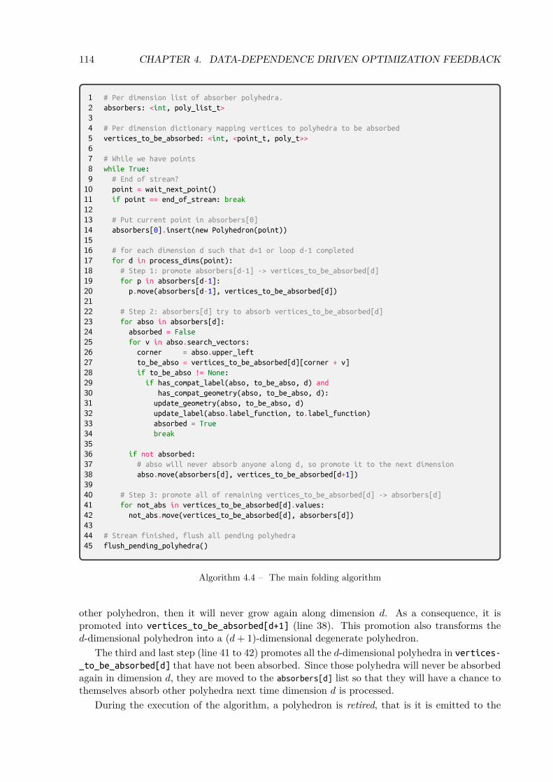
114 CHAPTER 4. DATA-DEPENDENCE DRIVEN OPTIMIZATION FEEDBACK
1 # Per dimension list of absorber polyhedra.
2 absorbers: <int, poly_list_t>
34 # Per dimension dictionary mapping vertices to polyhedra to be absorbed
5 vertices_to_be_absorbed: <int, <point_t, poly_t>>
67 # While we have points
8 while True:
9 # End of stream?
10 point = wait_next_point()
11 if point == end_of_stream: break
1213 # Put current point in absorbers[0]
14 absorbers[0].insert(new Polyhedron(point))
1516 # for each dimension d such that d=1 or loop d-1 completed
17 for d in process_dims(point):
18 # Step 1: promote absorbers[d-1] -> vertices_to_be_absorbed[d]
19 for p in absorbers[d-1]:
20 p.move(absorbers[d-1], vertices_to_be_absorbed[d])
2122 # Step 2: absorbers[d] try to absorb vertices_to_be_absorbed[d]
23 for abso in absorbers[d]:
24 absorbed = False
25 for v in abso.search_vectors:
26 corner = abso.upper_left
27 to_be_abso = vertices_to_be_absorbed[d][corner + v]
28 if to_be_abso != None:
29 if has_compat_label(abso, to_be_abso, d) and
30 has_compat_geometry(abso, to_be_abso, d):
31 update_geometry(abso, to_be_abso, d)
32 update_label(abso.label_function, to.label_function)
33 absorbed = True
34 break
3536 if not absorbed:
37 # abso will never absorb anyone along d, so promote it to the next dimension
38 abso.move(absorbers[d], vertices_to_be_absorbed[d+1])
3940 # Step 3: promote all of remaining vertices_to_be_absorbed[d] -> absorbers[d]
41 for not_abs in vertices_to_be_absorbed[d].values:
42 not_abs.move(vertices_to_be_absorbed[d], absorbers[d])
4344 # Stream finished, flush all pending polyhedra
45 flush_pending_polyhedra()
Algorithm 4.4 – The main folding algorithm
other polyhedron, then it will never grow again along dimension d. As a consequence, it ispromoted into vertices_to_be_absorbed[d+1] (line 38). This promotion also transforms thed-dimensional polyhedron into a (d+ 1)-dimensional degenerate polyhedron.
The third and last step (line 41 to 42) promotes all the d-dimensional polyhedra in vertices-
_to_be_absorbed[d] that have not been absorbed. Since those polyhedra will never be absorbedagain in dimension d, they are moved to the absorbers[d] list so that they will have a chance tothemselves absorb other polyhedra next time dimension d is processed.
During the execution of the algorithm, a polyhedron is retired, that is it is emitted to the
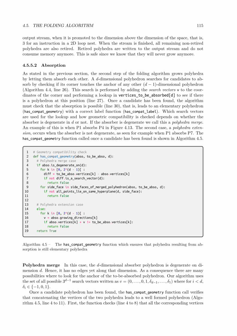
4.5. THE FOLDING ALGORITHM 115
output stream, when it is promoted to the dimension above the dimension of the space, that is,3 for an instruction in a 2D loop nest. When the stream is finished, all remaining non-retiredpolyhedra are also retired. Retired polyhedra are written to the output stream and do notconsume memory anymore. This is safe since we know that they will never grow anymore.
4.5.5.2 Absorption
As stated in the previous section, the second step of the folding algorithm grows polyhedraby letting them absorb each other. A d-dimensional polyhedron searches for candidates to ab-sorb by checking if its corner touches the anchor of any other (d − 1)-dimensional polyhedron(Algorithm 4.4, line 26). This search is performed by adding the search vectors v to the coor-dinates of the corner and performing a lookup in vertices_to_be_absorbed[d] to see if thereis a polyhedron at this position (line 27). Once a candidate has been found, the algorithmmust check that the absorption is possible (line 30), that is, leads to an elementary polyhedron(has_compat_geometry) with a correct label function (has_compat_label). Which search vectorsare used for the lookup and how geometric compatibility is checked depends on whether theabsorber is degenerate in d or not. If the absorber is degenerate we call this a polyhedra merge.An example of this is when P1 absorbs P4 in Figure 4.13. The second case, a polyhedra exten-sion, occurs when the absorber is not degenerate, as seen for example when P1 absorbs P7. Thehas_compat_geometry function called once a candidate has been found is shown in Algorithm 4.5.
1 # Geometry compatibility check
2 def has_compat_geometry(abso, to_be_abso, d):
3 # Polyhedra merge case
4 if abso.is_degenerate_on(d):
5 for k in [0, 2^(d - 1)[ :
6 diff = to_be_abso.vertices[k] - abso.vertices[k]
7 if not diff.is_a_search_vector(d):
8 return False
9 for side_face in side_faces_of_merged_polyhedron(abso, to_be_abso, d):
10 if not all_points_lie_on_same_hyperplane(d, side_face):
11 return False
1213 # Polyhedra extension case
14 else:
15 for k in [0, 2^(d - 1)[ :
16 v = abso.growing_directions[k]
17 if abso.vertices[k] + v != to_be_abso.vertices[k]:
18 return False
19 return True
Algorithm 4.5 – The has_compat_geometry function which ensures that polyhedra resulting from ab-sorption is still elementary polyhedra
Polyhedra merge In this case, the d-dimensional absorber polyhedron is degenerate on di-mension d. Hence, it has no edges yet along that dimension. As a consequence there are manypossibilities where to look for the anchor of the to-be-absorbed polyhedron. Our algorithm usesthe set of all possible 3d−1 search vectors written as v = (0, . . . , 0, 1, δd−1, . . . , δ1) where for i < d,δi ∈ {−1, 0, 1}.
Once a candidate polyhedron has been found, the has_compat_geometry function call verifiesthat concatenating the vertices of the two polyhedra leads to a well formed polyhedron (Algo-rithm 4.5, line 4 to 11). First, the function checks (line 4 to 8) that all the corresponding vertices

116 CHAPTER 4. DATA-DEPENDENCE DRIVEN OPTIMIZATION FEEDBACK
of both polyhedra are connected through the search vectors used to find the anchor of the to-be-absorbed polyhedron described just above. Second, the function checks (line 9 to line 11)that all the side faces of the polyhedron resulting from the absorption are valid. As shown inFigure 4.15, even if the lower (a square) and the upper (a triangle) faces are valid elementarypolyhedra, the result of the absorption may not be a valid polyhedron. For this we check if allthe points of the side face lie on the same hyperplane (line 11). To begin with, we arbitrarilydesignate one point of the face as the origin of the plane. We then pick d − 1 other points tocalculate a normal vector n for the plane by calculating the nullspace of the space spanned bythe vectors from the origin to the other points. And finally, we verify for all remaining points pthat the dot product (origin− p) · n equals zero.
cjck
ci
Figure 4.15 – Example of invalid polyhedron after absorption
If absorption is performed, the resulting polyhedron will no longer be degenerate in d. By con-struction, if well formed, the so obtained polyhedron is necessarily an elementary d-dimensionalpolyhedron. Its lower face will be the original absorbing polyhedron while its upper face will bethe the absorbed polyhedron.
Polyhedra extension In this case the absorber is a non-degenerate d-dimensional polyhedron.Hence, the absorber already has edges along dimension d. When looking for candidates to absorb,there is only one search vector, the edge connecting the oldest vertex of the lower face to that ofthe upper face. To check if the absorption is legal, has_compat_geometry simply verifies (line 14to line 18) whether the vertices of the two polyhedra can be connected using the existing edgesof the absorber stored in the growing_directions list.
4.5.5.3 Compatibility and update of label functions
The absorption is performed only if both geometric and label compatibility are satisfied (line 30).This section describes how label functions are represented, created and combined together.
Label functions The data structure used for label functions is shown in Figure 4.16. num-
_dimensions is the number of loops enclosing the static instruction or the destination instructionassociated with the input stream.
Creation Label functions are created when a new polyhedron is created from a single point(line 14). At this time, all the coefficients of the function are still unknown. Their typesin the coeff_types array are set to ⊥. The coordinates of the point used to create the newpolyhedron are saved in the initial_point array. The first cell of this array is never used butstill kept to make accesses more readable, that is, initial_point[d] contains the dth coordinate.

4.5. THE FOLDING ALGORITHM 117
enum Coefficient_Type:
⊥, # coefficient undetermined
INT, # coefficient determined
> # coefficient widened
struct Label_Function:
num_dimensions: int
init_point: int[num_dimensions + 1]
coeffs: int[num_dimensions + 1]
coeff_types: Coefficient_Type[num_dimensions + 1]
Figure 4.16 – The data structure used to represent label functions
These coordinates are used when coefficients are updated. Note that once a coefficient has beenupdated from an unknown to a known value, it is never updated again except to be set to >.The life cycle of a coefficient is then the following one:
⊥ → Z → >
At creation time, coeff[0] is given the value of the label associated with the initial point.As long as there are some ⊥ coefficients, coeff[0] contains the remaining amount contributedby unknown coefficients. We refer to coeff[0] as the remaining value in the following. Thisremaining value is updated whenever a coefficient is updated. When all coefficients are known,the remaining value represents the constant coefficient of the affine function.
The two polyhedra involved in a compatibility check along dimension d may be degenerate onone or more dimensions, including the dth one. As a consequence, the check may be faced withaffine functions where some coefficients are ⊥. In the following, we note the label function ofthe absorbing polyhedron as f_abso, and that of the polyhedron to be absorbed as f_to_be_abso.We notice that the polyhedron to be absorbed is always degenerate on dimension d, as statedin Section 4.5.5.1. Hence, f_to_be_abso.coeff_types[d] = ⊥.
All dimensions below are known For illustrative purposes we first cover the simplified casewhere all dimensions below d are known for the two label functions. The compatibility checkfor this simple case is shown in Algorithm 4.6. First the function has_compat_label verifies thatall coefficients for dimensions from 1 to d− 1 are the same. If this is not the case the two labelfunctions are incompatible (line 6).
Otherwise, the check may be faced with two cases corresponding to the two different ab-sorption cases described in Section 4.5.5.2. In the polyhedra merge case, where the absorberpolyhedron is degenerate on dimension d, that is, f_abso.coeff_types[d] = ⊥, the check al-ways succeeds and the has_compat_label function returns True (line 10). Indeed, by setting theproper coefficient for dimension d and by updating the remaining value, it is always possible tomake the two functions compatible as shown by the update_label function in Algorithm 4.6. Thenew coefficient is equal to the difference of remaining values (line 22). Note that, in general wewould also have to divide the new coefficient by the progress made along dimension d. However,because absorption guarantees that the two polyhedra whose label functions are being mergedtouch each other the progress is always equal to 1. Finally, the remaining value is decreasedby the effective contribution of the new coefficient taking into account the dth coordinate of theinitial point (line 28).
In the polyhedra extension case, the absorber polyhedron is not degenerate on dimensiond. Its affine function already has a value computed for the coefficient on dimension d. Then

118 CHAPTER 4. DATA-DEPENDENCE DRIVEN OPTIMIZATION FEEDBACK
1 # Compatibility check when all dimensions below d are known
2 def has_compat_label(f_abso, f_to_be_abso, d):
3 # Verifies coefficients below d are the same
4 for q in range [1, d-1]:
5 if f_abso.coeffs[q] != f_to_be_abso.coeffs[q]:
6 return False
78 # Polyhedra merge case
9 if f_abso.coeffs[d] == ⊥:
10 return True
1112 # Polyhedra extension case
13 else:
14 new_coeff_contrib = f_abso.coeffs[d] * f_to_be_abso.coeffs[d]
15 new_remain = f_to_be_abso.coeffs[0] - new_coeff_contrib
16 return new_remain == f_abso.coeffs[0]
1718 # Update coefficient for dimension d and remaining value of f_abso.
19 # No need to update f_to_be_abso because it will be thrown after absorption
20 def update_label(f_abso, f_to_be_abso, d):
21 # Update of coefficient
22 new_coeff = f_to_be_abso.coeffs[0] - f_abso.coeffs[0]
23 f_abso.coeffs[d] = new_coeff
24 f_abso.coeff_types[d] = INT
2526 # Update of remaining value
27 new_coeff_contrib = new_coeff * f_abso.init_point[d]
28 f_abso.coeffs[0] = f_abso.coeffs[0] - new_coeff_contrib
Algorithm 4.6 – Simplified version of the compatibility check and update of coefficient for the casewhen all dimensions below d are known. See Algorithm 4.7 and Algorithm 4.8 for the general case ofhas_compat_label and update_label.
f_{abs}.coeff_types[d] 6= ⊥ and nothing needs to be updated. The compatibility check mustonly ensure that this coefficient is compatible with f_to_be_abso. This is done by first computingthe contribution of the known coefficient of f_abso into f_to_be_abso using the initial point off_to_be_abso (line 14). Then, the check subtracts this contribution from the remaining valueof f_to_be_abso to compute its new remaining value. For the check to return true, this newremaining value must be equal to the remaining value of f_abso (line 16).
General case In the general case the two polyhedra may be degenerate for some dimensionsbelow d. This happens if a dimension below d only iterates once. The compatibility checkdescribed above must take this into account.
Function has_compat_label in Algorithm 4.7 shows the general compatibility check betweentwo polyhedra. The check is performed on all the matching pairs of label functions of the twopolyhedra. Remember that there are several such label functions in the case of dependencies,one for each dimension of the source instruction.
The check works by comparing the coefficients of both functions for all the dimensions from1 to d. If both coefficients for a dimension are known they must be the same or the check fails(line 15). If one is known and not the other (line 20 and line 24), then the function incrementsthe total contribution coming from the other function for the function having the unknowncoefficient. At the end of the loop (line 33), the check ensures that the coefficient for dimensiond in f_abso is compatible with f_to_be_abso. This check relies on the total contribution variables
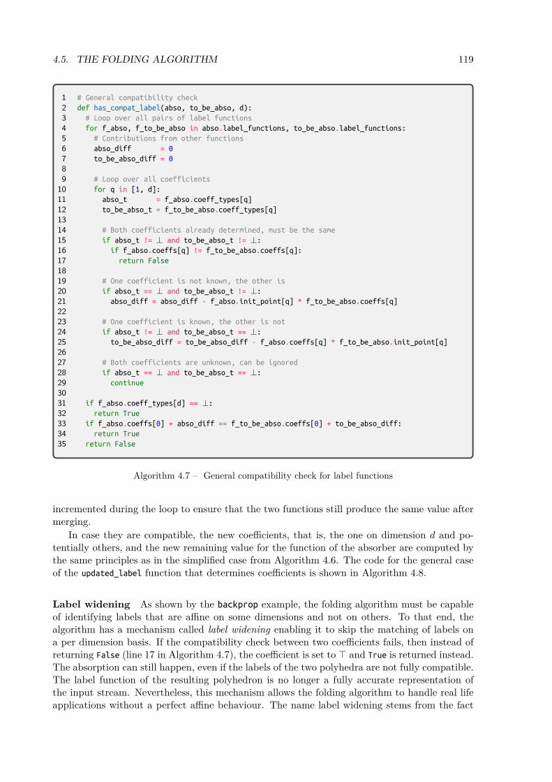
4.5. THE FOLDING ALGORITHM 119
1 # General compatibility check
2 def has_compat_label(abso, to_be_abso, d):
3 # Loop over all pairs of label functions
4 for f_abso, f_to_be_abso in abso.label_functions, to_be_abso.label_functions:
5 # Contributions from other functions
6 abso_diff = 0
7 to_be_abso_diff = 0
89 # Loop over all coefficients
10 for q in [1, d]:
11 abso_t = f_abso.coeff_types[q]
12 to_be_abso_t = f_to_be_abso.coeff_types[q]
1314 # Both coefficients already determined, must be the same
15 if abso_t != ⊥ and to_be_abso_t != ⊥:
16 if f_abso.coeffs[q] != f_to_be_abso.coeffs[q]:
17 return False
1819 # One coefficient is not known, the other is
20 if abso_t == ⊥ and to_be_abso_t != ⊥:
21 abso_diff = abso_diff - f_abso.init_point[q] * f_to_be_abso.coeffs[q]
2223 # One coefficient is known, the other is not
24 if abso_t != ⊥ and to_be_abso_t == ⊥:
25 to_be_abso_diff = to_be_abso_diff - f_abso.coeffs[q] * f_to_be_abso.init_point[q]
2627 # Both coefficients are unknown, can be ignored
28 if abso_t == ⊥ and to_be_abso_t == ⊥:
29 continue
3031 if f_abso.coeff_types[d] == ⊥:
32 return True
33 if f_abso.coeffs[0] + abso_diff == f_to_be_abso.coeffs[0] + to_be_abso_diff:
34 return True
35 return False
Algorithm 4.7 – General compatibility check for label functions
incremented during the loop to ensure that the two functions still produce the same value aftermerging.
In case they are compatible, the new coefficients, that is, the one on dimension d and po-tentially others, and the new remaining value for the function of the absorber are computed bythe same principles as in the simplified case from Algorithm 4.6. The code for the general caseof the updated_label function that determines coefficients is shown in Algorithm 4.8.
Label widening As shown by the backprop example, the folding algorithm must be capableof identifying labels that are affine on some dimensions and not on others. To that end, thealgorithm has a mechanism called label widening enabling it to skip the matching of labels ona per dimension basis. If the compatibility check between two coefficients fails, then instead ofreturning False (line 17 in Algorithm 4.7), the coefficient is set to > and True is returned instead.The absorption can still happen, even if the labels of the two polyhedra are not fully compatible.The label function of the resulting polyhedron is no longer a fully accurate representation ofthe input stream. Nevertheless, this mechanism allows the folding algorithm to handle real lifeapplications without a perfect affine behaviour. The name label widening stems from the fact

120 CHAPTER 4. DATA-DEPENDENCE DRIVEN OPTIMIZATION FEEDBACK
1 # Update coefficient for all dimensions <= d and remaining value of f_abso.
2 # No need to update f_to_be_abso because it will be thrown after absorption
3 def update_label(abso, to_be_abso, d):
4 # Loop over all pairs of label functions
5 for f_abso, f_to_be_abso in abso.label_functions, to_be_abso.label_functions:
6 abso_diff = 0
7 to_be_abso_diff = 0
89 for q in range(1, q + 1):
10 abso_t = f_abso.coeff_types[q]
11 to_be_abso_t = f_to_be_abso.coeff_types[q]
1213 # One coefficient is not known, the other is
14 if abso_t == ⊥ and to_be_abso_t != ⊥:
15 abso_diff = abso_diff - f_abso.init_point[q] * f_to_be_abso.coeffs[q]
16 set_coefficient(f_abso, f_to_be_abso.coeffs[q], q)
1718 # One coefficient is known, the other is not
19 if abso_t != ⊥ and to_be_abso_t == ⊥:
20 to_be_abso_diff = to_be_abso_diff - f_abso.coeffs[q] * f_to_be_abso.init_point[q]
2122 # Both coefficients are unknown, can be ignored
23 if abso_t == ⊥ and to_be_abso_t == ⊥:
24 continue
2526 if f_abso.coeff_types[d] == ⊥:
27 new_coeff = to_be_abso_diff - f_to_be_abso.coeffs[0] - f_abso.coeffs[0]
28 set_coefficient(f_abso, new_coeff, q)
2930 def set_coefficient(fn, coeff_val: int, q: Dimension):
31 delta = -coeff_val * self.init_point[q]
32 fn.coeff_types[q] = INT
33 fn.coeffs[q] = coeff_val
34 fn.coeffs[0] = fn.coeffs[0] + delta
Algorithm 4.8 – General case for determining coefficients of label functions
that in the case of dependencies it widens the label functions from equalities to inequalities, asshown in Section 4.5.3.
The integration of this feature into Algorithm 4.7 is straightforward. A > coefficient iscompatible with any other coefficient, and when performing absorption, any such coefficient inone of the two label functions leads to a > coefficient in the updated function.
The label widening mechanism is crucial for the label functions of instructions because >is a clear indicator that a memory access is not affine along a dimension. For dependencies itsimply reduces the size of the output given to the back-end by reducing the number of producedpieces.
4.5.5.4 Geometric give up
Even with the label widening mechanism described above, some applications may lead to thecreation of a huge number of polyhedra. This happens when the geometry of instructionsand dependencies are not affine. It occurs for statements surrounded by if conditionals in theprogram. In the worst case, the folding algorithm creates one polyhedron for each dynamicinstruction and for each dynamic dependency.
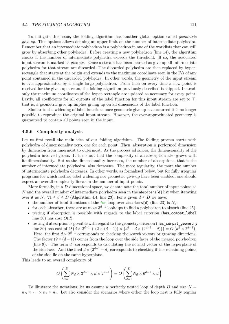
4.5. THE FOLDING ALGORITHM 121
To mitigate this issue, the folding algorithm has another global option called geometricgive-up. This options allows defining an upper limit on the number of intermediate polyhedra.Remember that an intermediate polyhedron is a polyhedron in one of the worklists that can stillgrow by absorbing other polyhedra. Before creating a new polyhedron (line 14), the algorithmchecks if the number of intermediate polyhedra exceeds the threshold. If so, the associatedinput stream is marked as give up. Once a stream has been marked as give up all intermediatepolyhedra for that stream are discarded. The discarded polyhedra are then replaced by hyper-rectangle that starts at the origin and extends to the maximum coordinate seen in the IVs of anypoint contained in the discarded polyhedra. In other words, the geometry of the input streamis over-approximated by a single large polyhedron. From then on every time a new point isreceived for the given up stream, the folding algorithm previously described is skipped. Instead,only the maximum coordinates of the hyper-rectangle are updated as necessary for every point.Lastly, all coefficients for all outputs of the label function for this input stream are set to >,that is, a geometric give up implies giving up on all dimensions of the label function.
Similar to the widening of label functions once geometric give up has occurred it is no longerpossible to reproduce the original input stream. However, the over-approximated geometry isguaranteed to contain all points seen in the input.
4.5.6 Complexity analysis
Let us first recall the main idea of our folding algorithm. The folding process starts withpolyhedra of dimensionality zero, one for each point. Then, absorption is performed dimensionby dimension from innermost to outermost. As the process advances, the dimensionality of thepolyhedra involved grows. It turns out that the complexity of an absorption also grows withits dimensionality. But as the dimensionality increases, the number of absorptions, that is thenumber of intermediate polyhedra, also decreases. The more regularity, the more the numberof intermediate polyhedra decreases. In other words, as formalised below, but for fully irregularprograms for which neither label widening nor geometric give-up have been enabled, one shouldexpect an overall complexity linear in the number of input points.
More formally, in a D-dimensional space, we denote note the total number of input points asN and the overall number of intermediate polyhedra seen in the absorbers[d] list when iteratingover it as Nd, ∀1 ≤ d ≤ D (Algorithm 4.4, line 23). For a given d ≤ D we have:
• the number of total iterations of the for loop over absorbers[d] (line 23) is Nd;• for each absorber, there are at most 3d−1 look-ups to find a polyhedron to absorb (line 25);• testing if absorption is possible with regards to the label criterion (has_compat_label
line 30) has cost O(d);• testing if absorption is possible with regard to the geometry criterion (has_compat_geometry
line 30) has cost of O(d× 2d−1 + (2× (d− 1))×
(d3 + d× (2d−1 − d)
))= O
(d2 × 2d−1
).
Here, the first d× 2d−1 corresponds to checking the search vectors or growing directions.The factor (2× (d− 1)) comes from the loop over the side faces of the merged polyhedron(line 9). The term d3 corresponds to calculating the normal vector of the hyperplane ofthe sideface. And the final d× (2d−1 − d) corresponds to checking if the remaining pointsof the side lie on the same hyperplane.
This leads to an overall complexity of:
O
(D∑
d=1
Nd × 3d−1 × d× 2d−1
)= O
(D∑
d=1
Nd × 6d−1 × d
)
To illustrate the notations, let us assume a perfectly nested loop of depth D and size N =nD × · · · × n2 × n1. Let also consider the scenarios where either the loop nest is fully regular
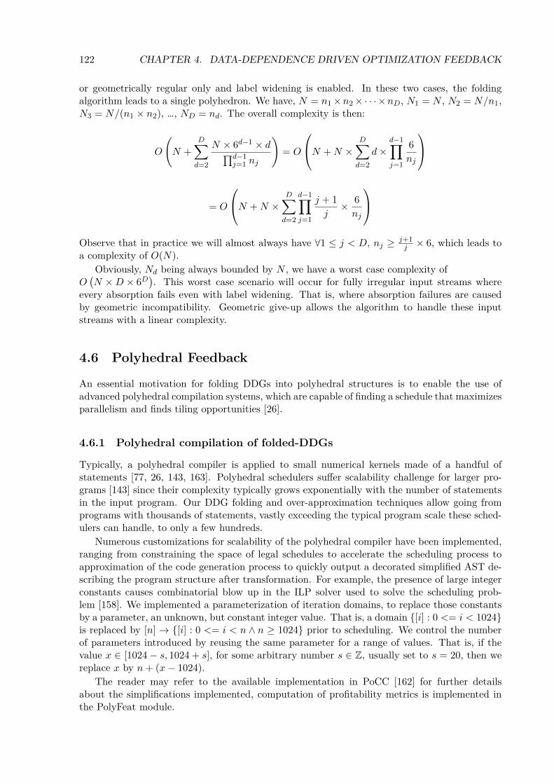
122 CHAPTER 4. DATA-DEPENDENCE DRIVEN OPTIMIZATION FEEDBACK
or geometrically regular only and label widening is enabled. In these two cases, the foldingalgorithm leads to a single polyhedron. We have, N = n1×n2×· · ·×nD, N1 = N , N2 = N/n1,N3 = N/(n1 × n2), …, ND = nd. The overall complexity is then:
O
(N +
D∑d=2
N × 6d−1 × d∏d−1j=1 nj
)= O
N +N ×D∑
d=2
d×d−1∏j=1
6
nj
= O
N +N ×D∑
d=2
d−1∏j=1
j + 1
j× 6
nj
Observe that in practice we will almost always have ∀1 ≤ j < D, nj ≥ j+1
j × 6, which leads toa complexity of O(N).
Obviously, Nd being always bounded by N , we have a worst case complexity ofO(N ×D × 6D
). This worst case scenario will occur for fully irregular input streams where
every absorption fails even with label widening. That is, where absorption failures are causedby geometric incompatibility. Geometric give-up allows the algorithm to handle these inputstreams with a linear complexity.
4.6 Polyhedral Feedback
An essential motivation for folding DDGs into polyhedral structures is to enable the use ofadvanced polyhedral compilation systems, which are capable of finding a schedule that maximizesparallelism and finds tiling opportunities [26].
4.6.1 Polyhedral compilation of folded-DDGs
Typically, a polyhedral compiler is applied to small numerical kernels made of a handful ofstatements [77, 26, 143, 163]. Polyhedral schedulers suffer scalability challenge for larger pro-grams [143] since their complexity typically grows exponentially with the number of statementsin the input program. Our DDG folding and over-approximation techniques allow going fromprograms with thousands of statements, vastly exceeding the typical program scale these sched-ulers can handle, to only a few hundreds.
Numerous customizations for scalability of the polyhedral compiler have been implemented,ranging from constraining the space of legal schedules to accelerate the scheduling process toapproximation of the code generation process to quickly output a decorated simplified AST de-scribing the program structure after transformation. For example, the presence of large integerconstants causes combinatorial blow up in the ILP solver used to solve the scheduling prob-lem [158]. We implemented a parameterization of iteration domains, to replace those constantsby a parameter, an unknown, but constant integer value. That is, a domain {[i] : 0 <= i < 1024}is replaced by [n] → {[i] : 0 <= i < n ∧ n ≥ 1024} prior to scheduling. We control the numberof parameters introduced by reusing the same parameter for a range of values. That is, if thevalue x ∈ [1024− s, 1024 + s], for some arbitrary number s ∈ Z, usually set to s = 20, then wereplace x by n+ (x− 1024).
The reader may refer to the available implementation in PoCC [162] for further detailsabout the simplifications implemented, computation of profitability metrics is implemented inthe PolyFeat module.
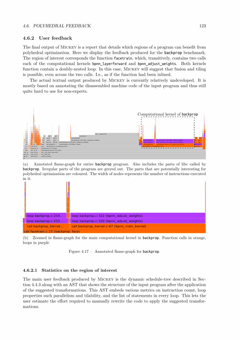
4.6. POLYHEDRAL FEEDBACK 123
4.6.2 User feedback
The final output of Mickey is a report that details which regions of a program can benefit frompolyhedral optimization. Here we display the feedback produced for the backprop benchmark.The region of interest corresponds the function facetrain, which, transitively, contains two callseach of the computational kernels bpnn_layerforward and bpnn_adjust_weights. Both kernelsfunction contain a doubly-nested loop. In this case, Mickey will suggest that fusion and tilingis possible, even across the two calls. I.e., as if the function had been inlined.
The actual textual output produced by Mickey is currently relatively undeveloped. It ismostly based on annotating the disassembled machine code of the input program and thus stillquite hard to use for non-experts.
all
call ini..
call _dl..
call _d..
cal..
lo..
lo..
ca..
ca..
c..
c..
call init_ tls..
loop _dl_ ini..
loop _dl_ ini..
call _dl_ ini..
loop call_ in..
call call_ in..
cal..
call init_ tls+452
call _start+36
call __ libc_start_main+232
call backprop_kernel.c:42 (main)
call facetrain.c:47 (setup)
call ..
loop ..
cal..
cal..
cal..
c..
call facetrain.c:22 (backprop_ face)
call backprop.c: ..
loop ba..
call b..
call 0..
call..
loop ba..
call b..
call 0..
call..
loop backprop.c:216 (bpnn_create)
loop backprop.c:100 (bpnn_randomize_weights)
call backprop.c:100 (bpnn_randomize_weights)
call 0x400a80
call rand+4
call __ random+93
lo..
ca..
c..
call facetrain.c:27 (backprop_ face)
call backprop_k..
loop backprop.c..
loop backprop...
call backprop_kernel.c:67 (bpnn_train_kernel)
loop backprop.c:320 (bpnn_adjust_weights)
loop backprop.c:322 (bpnn_adjust_weights)
call facet..
loop backp..
cal..
cal..
ca..
call..
call..
ca..
c..
c..
Computational kernel of backprop
(a) Annotated flame-graph for entire backprop program. Also includes the parts of libc called bybackprop. Irregular parts of the program are greyed out. The parts that are potentially interesting forpolyhedral optimization are coloured. The width of nodes represents the number of instructions executedin it.
call facetrain.c:27 (backprop_ face)
call backprop_kernel...
loop backprop.c:253 ..
loop backprop.c:254..
call backprop_kernel.c:67 (bpnn_train_kernel)
loop backprop.c:320 (bpnn_adjust_weights)
loop backprop.c:322 (bpnn_adjust_weights)
(b) Zoomed in flame-graph for the main computational kernel in backprop. Function calls in orange,loops in purple
Figure 4.17 – Annotated flame-graph for backprop.
4.6.2.1 Statistics on the region of interest
The main user feedback produced by Mickey is the dynamic schedule-tree described in Sec-tion 4.4.3 along with an AST that shows the structure of the input program after the applicationof the suggested transformations. This AST embeds various metrics on instruction count, loopproperties such parallelism and tilability, and the list of statements in every loop. This lets theuser estimate the effort required to manually rewrite the code to apply the suggested transfor-mations.

124 CHAPTER 4. DATA-DEPENDENCE DRIVEN OPTIMIZATION FEEDBACK
To better visualize the various program regions, this information can be rendered as a flame-graph[79]. This flame-graph is a hierarchic representation of the structure of a program. Thatis, a tree where each node represents one region of code, either a loop or a function. Thechildren of a node are the functions called from that code region or the loops contained init. In this visualization the width of a node is proportional to its estimated computationalhotness, determined by the number of instructions it executed. Colours and gradients are usedto encode the estimated potential for optimization detected by Mickey. Non-interesting regions,for example, can be greyed out. These flame-graphs are SVG files, which can be clicked andzoomed to obtain detailed information on each region. An example flame-graph, created frombackprop, can be seen in Figure 4.17.
We also display explicit statistics for each region, breaking down by instruction type, asshown in Figure 4.18. The statistics are computed automatically from the folded DDG byreasoning on the number of points in each iteration domain/dependence, and the associatedassembly instructions.
Statistics on the instruction mix are useful in particular to estimate the operational intensityas the ratio of load/store operations per total non-memory operations. Besides Mickey further-more reports how many instructions each different loop level contains to highlight the potentialimpact of transformations across deep loop nests. We also compute the values for these metricsassuming the proposed transformation had been implemented. This is intended to assist theuser in determining the potential benefit of a transformation.
Number of iteration domains: 69
Number of dependence polyhedra: 76
Totals: 6816353 operations, 6816434 operation-to-operation dependences
Total operations: 6816353
Total FLOPs: 3670321 (53.85%)
Total load/store: 3145965 (46.15%)
Total INT: 50 (0.00%)
Total others: 17 (0.00%)
Maximal loop depth: 2
-> depth=0: 0 instructions (0.00%) 0 operations (0.00%)
-> depth=1: 40 instructions (57.97%) 340 operations (0.00%)
-> depth=2: 29 instructions (42.03%) 6816013 operations (100.00%)
Figure 4.18 – Statistics on the fat region of interest
4.6.2.2 Transformations feedback: simplified AST after transformation
A key feedback provided to the user is a simplified AST that displays the code structure afterapplying the suggested transformation. Figure 4.19 shows an excerpt of this AST.
This AST obeys the following principles:1. All statistics on the number of operations and percentages shown are cumulative, i.e., they
represent the total number of operations dominated by a node. Similarly, the statementlist is also cumulative, i.e., it captures all statements under a node, wherever they arelocated in the sub-tree.
2. Loops in the output program are always named i′, j′, k′, l, l′, . . .3. A loop can have the following attributes: sequential, or parallel. The tilable qualifier can
appear for both parallel and sequential loops. A tilable loop is necessarily permutablewith any other tilable loop in the same loop nest. A sequential/tilable loop necessarily

4.6. POLYHEDRAL FEEDBACK 125
...
|= AST=(0,0,i')
|-- Loop i' => parallel/tilable loop, 2097203 operations (30.77%)
+-- alignment: 3 stride-0 (524322) 2 stride-1 (1048576) 0 stride-N (0)
|-- contains: S64 S67 S62 S65 S57 S54 S55
|-- Stmts full names:
+ 4011800000000101_4011bf(c0,c1); // LOAD
+ 4011800000000101_4011cb(c0,c1); // LOAD
+ 4011800000000101_4011ac(c0,c1); // LOAD
+ 4011800000000101_4011c3(c0,c1); // FLOAT
+ 4011800000000001_4011cb(c0,c1); // LOAD
+ 4011800000000001_4011bf(c0,c1); // LOAD
+ 4011800000000001_4011c3(c0,c1); // FLOAT
|= AST=(0,0,i',j')
|-- Loop j' => parallel/tilable loop, 2097203 operations (30.77%)
+-- alignment: 1 stride-0 (524288) 0 stride-1 (0) 4 stride-N (1048610)
|-- contains: S64 S67 S62 S65 S57 S54 S55
|-- Stmts full names:
+ 4011800000000101_4011bf(c0,c1); // LOAD
+ 4011800000000101_4011cb(c0,c1); // LOAD
+ 4011800000000101_4011ac(c0,c1); // LOAD
+ 4011800000000101_4011c3(c0,c1); // FLOAT
+ 4011800000000001_4011cb(c0,c1); // LOAD
+ 4011800000000001_4011bf(c0,c1); // LOAD
+ 4011800000000001_4011c3(c0,c1); // FLOAT
|= AST=(0,6,i')
|-- Loop i' => parallel/tilable loop, 1048576 operations (15.38%)
+-- alignment: 2 stride-0 (1048576) 0 stride-1 (0) 0 stride-N (0)
|-- contains: S3 S4
...
Figure 4.19 – Excerpt of simplified AST produced for backprop
only has forward dependencies. A sequential, but not tilable, loop may or may not haveonly forward dependencies, i.e., be permutable with other loops. A parallel is alwayssinkable to any lower loop level, including the last one, independent of any tilability.
4. The alignment information for memory accesses is populated only if the input DDG hasinformation about access functions. If the label function describing the memory accesseshas only > coefficients then 0 will be printed everywhere.
5. The alignment information displayed for a loop shows how often different memory accessstrides occur in that loop if it where transformed to be an inner-most loop. This gives theuser an indication of the profitability of loop interchanges. For example for the purposeof vectorization as has been shown in the backprop example. Note, however that it is notalways possible to sink a loop to be inner-most. This is only possible for loops marked asparallel.
6. The statements in the “Stmt full names” list appear in their prefix order in the AST.That is, the order in which they will syntactically occur in the transformed code.
7. The Kelly’s mapping style iteration vector |= AST=(0,i',j') displayed for each nodevisualizes its position in the AST. The first component represents the root of the schedule

126 CHAPTER 4. DATA-DEPENDENCE DRIVEN OPTIMIZATION FEEDBACK
tree and is always 0. This is then followed by an arbitrary sequence of constant numbersand loop iterators. Nodes are displayed in the order of a prefix traversal of the scheduletree, i.e., by increasing lexicographic order.
4.6.2.3 Transformations feedback: transformed pseudo-code
Technically, Mickey does not only determine the existence of a loop transformation sequenceto implement parallelism and locality: it also generates the code structure that is the resultof this transformation. This representation of the transformed program can be pretty-printedas pseudo-code. The C-like pseudo code is intended to help users with implementing morecomplicated loop transformations.
Figure 4.20 shows an example of this pseudo-code for a part of backprop, where a tiling ofsize 32x32 was found and implemented. Each statement in this pseudo-code corresponds to onemachine instruction of the original program. We also attach annotations to loops and statementsto show about the properties of each loop. For example if a loop is parallel or not. The user caninspect this code to understand which statements should be grouped together under the sameloop nest to implement fusion.
...
parallel for (jTile = 0; jTile <= floor(32767/32); jTile++) {
for (i = 0; i <= 15; i++) {
parallel for (j = (32 * jTile); j <= min(32767, ((32 * jTile) + 31)); j++) {
4012280000000101_401249(i, j); /* @LOAD@ */;
4012280000000101_40125e(i, j); /* @FLOAT@ */;
4012280000000101_401265(i, j); /* @FLOAT@ */;
4012280000000101_401275(i, j); /* @FLOAT@ */;
4012280000000101_40127d(i, j); /* @FLOAT@ */;
4012280000000101_401289(i, j); /* @STORE@ */;
4012280000000101_401281(i, j); /* @FLOAT@ */;
4012280000000101_401285(i, j); /* @STORE@ */;
}
}
}
...
Figure 4.20 – Excerpt of transformed pseudo-code produced for backprop. Each statement consists ofa loop-call context tree node ID, 4012280000000101, and an instruction PC. For example 401249.
Statement names, e.g., 4012280000000101_401249, are composed of the ID of a context treeID, 4012280000000101, and an instruction PC, 401249. We also emit separate context includesdetails about all ASM instructions, such as the original source file and line for this instructionsmaps to. Note that displaying the ASM instruction and not only its type is possible, but notshown here for simplicity.
The user can inspect this pseudo-code at a high-level, only looking at the loop structure andthe attributes of the loops. Or they can “zoom in” to understand which statements should begrouped together, how complex the loop bounds may need to be, what range they take, and soon.
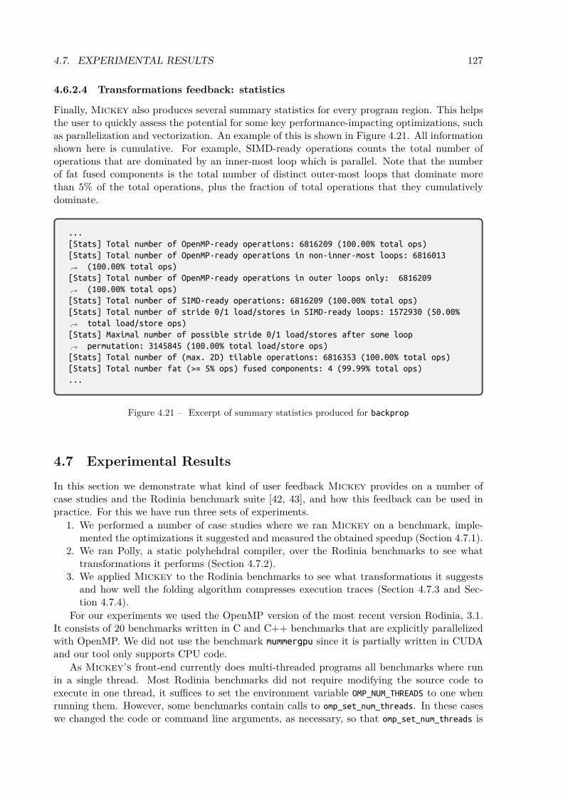
4.7. EXPERIMENTAL RESULTS 127
4.6.2.4 Transformations feedback: statistics
Finally, Mickey also produces several summary statistics for every program region. This helpsthe user to quickly assess the potential for some key performance-impacting optimizations, suchas parallelization and vectorization. An example of this is shown in Figure 4.21. All informationshown here is cumulative. For example, SIMD-ready operations counts the total number ofoperations that are dominated by an inner-most loop which is parallel. Note that the numberof fat fused components is the total number of distinct outer-most loops that dominate morethan 5% of the total operations, plus the fraction of total operations that they cumulativelydominate.
...
[Stats] Total number of OpenMP-ready operations: 6816209 (100.00% total ops)
[Stats] Total number of OpenMP-ready operations in non-inner-most loops: 6816013
(100.00% total ops)↪→
[Stats] Total number of OpenMP-ready operations in outer loops only: 6816209
(100.00% total ops)↪→
[Stats] Total number of SIMD-ready operations: 6816209 (100.00% total ops)
[Stats] Total number of stride 0/1 load/stores in SIMD-ready loops: 1572930 (50.00%
total load/store ops)↪→
[Stats] Maximal number of possible stride 0/1 load/stores after some loop
permutation: 3145845 (100.00% total load/store ops)↪→
[Stats] Total number of (max. 2D) tilable operations: 6816353 (100.00% total ops)
[Stats] Total number fat (>= 5% ops) fused components: 4 (99.99% total ops)
...
Figure 4.21 – Excerpt of summary statistics produced for backprop
4.7 Experimental Results
In this section we demonstrate what kind of user feedback Mickey provides on a number ofcase studies and the Rodinia benchmark suite [42, 43], and how this feedback can be used inpractice. For this we have run three sets of experiments.
1. We performed a number of case studies where we ran Mickey on a benchmark, imple-mented the optimizations it suggested and measured the obtained speedup (Section 4.7.1).
2. We ran Polly, a static polyhehdral compiler, over the Rodinia benchmarks to see whattransformations it performs (Section 4.7.2).
3. We applied Mickey to the Rodinia benchmarks to see what transformations it suggestsand how well the folding algorithm compresses execution traces (Section 4.7.3 and Sec-tion 4.7.4).
For our experiments we used the OpenMP version of the most recent version Rodinia, 3.1.It consists of 20 benchmarks written in C and C++ benchmarks that are explicitly parallelizedwith OpenMP. We did not use the benchmark mummergpu since it is partially written in CUDAand our tool only supports CPU code.
As Mickey’s front-end currently does multi-threaded programs all benchmarks where runin a single thread. Most Rodinia benchmarks did not require modifying the source code toexecute in one thread, it suffices to set the environment variable OMP_NUM_THREADS to one whenrunning them. However, some benchmarks contain calls to omp_set_num_threads. In these caseswe changed the code or command line arguments, as necessary, so that omp_set_num_threads is

128 CHAPTER 4. DATA-DEPENDENCE DRIVEN OPTIMIZATION FEEDBACK
only ever called with an argument of 1.All Rodinia benchmarks and case studies where compiled using GCC 8.1.1. The version of
the front-end used for these experiments uses QEMU 3.1. Since this version of QEMU cannothandle AVX instructions we used the compiler flags -g -O2 -msse3. For speedup measurementsprograms where compiled using the Intel icc and ifort compilers (version 18.0.3, flags -Ofast-march=native -mtune=native). The measurements where taken on a machine with a Xeon IvyBridge CPU with two 6 core CPUs (24 hyperthreads total), each running at 2.1 GHz (GFlop/sare averaged over 50 runs).
All benchmarks where compiled for and run on x86 CPUs. Since many x86 instructions bothread or write memory and perform computations at the same time the instructions streams thatform the input of the folding algorithm are actually more complicated than the ones presentedin Section 4.5.1 and Table 4.1. In reality the label of an instruction can have multiple valuesto account both for the addresses accessed and the values produced. The label functions forinstructions thus potentially have multiple outputs as well, just like those for dependencies.
4.7.1 Case studies
This section aims to present case studies that illustrate how the feedback provided by Mickeycan concretely be used to speed up programs.
4.7.1.1 Case study I
This case study illustrates a simple feedback Mickey can provide to users. It shows how Mickeypinpoints the absence of dependencies along some existing orthogonal outer loop dimensions,which enables coarse-grain parallelism via OpenMP parallel pragmas.
We selected alexnet for this study, a deep convolutional neural network used for imageclassification. We exploit the ability of Mickey to discover loop structures, to report typicalruntime values to evaluate the profitability of the transformation, and to handle interproceduralanalysis in a robust way.
The version of alexnet we used [230] has five sequential convolutional layers each imple-mented by a call to a function called convolution. Each call to convolution uses a different inputsize, weights and convolutional kernel size. Furthermore, three of these five layers are split intwo, implemented by calling convolution twice, each time with only half of the input data. Asreported in Table 4.5, Mickey detects that the three outermost loops inside of convolution areparallel. It also detects that the two calls to convolution for the split layers can be performedin parallel.
We obtained the reported speedup by adding a single omp pragma parallel for on the out-ermost loop in convolution. To exploit the nested parallelism of the second layer we use adouble nested parallel region. Applying these transformations increases the performance from 1GFlop/s to 10.9 GFlop/s for the first layer and from 3.8 GFlop/s to 5.6 GFlop/s for the second.Note that convolution is a heavily bandwidth-bound problem and performance already tops outwhen using 12 of the 24 hyperthreads.
4.7.1.2 Case study II
This case study again illustrates a relatively simple feedback from Mickey. Here Mickey findsthat dependencies live within the first quartant [14]. This allows exposing data locality andfine-grain parallelism through a loop interchange.
For this study, we selected backprop, a supervised learning method used to train artificialneural networks extracted from the Rodinia benchmark suite [43]. In addition to what was out-lined in the previous case study, Mickey exploits its ability to associate an iteration vector with

4.7. EXPERIMENTAL RESULTS 129
Code region %ops omp parallel loops speedup
conv1 @ alexnet.cc:70 15% layers.cc:{227,229,230} 7.6 x
conv21 @ alexnet.cc:119 29% alexnet.cc:{119} 1.5 xconv22 @ alexnet.cc:120 layers.cc:{220,222,224}
Table 4.5 – Results of the alexnet case study. Reported line numbers are from debug information. %opsgives percentage of total number of instructions in program executed in a region. Suggested parallel loopsare represented using a set of line numbers. I.e. layers.cc:{227,229,230} is a 3D loop nest.
each memory access, and to match pointer values with scalar evolution. Since the scalar evolu-tion expressions for a memory access describe the addresses it reads/writes, they can be used todetect strided accesses along any dimension, which in turn can be used to detect vectorizationpotential.
The flame-graph provided by Mickey is reported in Figure 4.17 where the regions of interestare: 1. the first call (of two) to bpnn_layerfoward with a constant value of n2 = 16 ; 2. the last call(of two) of bpnn_adjust_weights with a constant value of ndelta = 16. Both functions contain a2D-nested-loop, called Llayer and Ladjust respectively. For both loop nests Mickey suggests aninterchange followed by vectorization. For example, see Llayer on Table 4.6 for which the twoloop dimensions are reported to be on lines 249 (outer) and 253 (inner) of file backprop.c: Theloop nest is fully permutable, that is, interchange is possible. Also, only the outermost loopis parallel, and there are more stride 0/1 accesses along the outermost dimension (100%) thanalong the innermost (50%).
To enable the suggested transformations, one needs to specialize the two interesting functioncalls and array expand the scalar sum. The other calls to bpnn_layerfoward and bpnn_adjust_weights
are left unchanged, since they (a) take up much less of the overall program runtime (b) havedifferent arguments and do not profit from the transformation. Applying the transformation im-proved, in our case, bpnn_layerfoward from 0.5 GFlop/s to 2.8 GFlop/s and bpnn_adjust_weights
from 0.3 GFlop/s to 5.1 GFlop/s.
Code region %ops loop parallel permutable %stride 0/1 speedup
backprop_kernel.c:52 14% backprop.c:249 yes yes 100% 5.3 x(Llayer) backprop.c:253 no yes 50%
backprop_kernel.c:57 46% backprop.c:321 yes yes 100% 7.8 x(Ladjust) backprop.c:322 yes yes 50%
Table 4.6 – Results of the backprop case study. Reported line numbers are from debug information. Thetwo loop nests, backprop.c:{249,253} and backprop.c:{321,322}, both profit from a loop interchangesince the outer loop has more stride 0/1 accesses.
4.7.1.3 Case study III
This case study illustrates an example of advanced feedback. By providing exact dependencevector “directions” Mickey shows that data locality and coarse-grain parallelism can be exposedthrough loop skewing and tiling.
For this study, we selected GemsFDTD, a finite difference time domain method from the SPECCPU2006 benchmark suite [92] written in Fortran90. Analysing Fortran code is not a problemfor Mickey as it works at the binary level. However, the compiler we used (gfortran-8.1.1)messes up the debug information, making it necessary for the user to shift the line numbersfor the provided code references by hand. This case study fully exploits Mickey’s ability to

130 CHAPTER 4. DATA-DEPENDENCE DRIVEN OPTIMIZATION FEEDBACK
model (and compress in a polyhedral form) the data dependencies, instead of simply checkingtheir existence/absence. This knowledge about the structure of dependencies allows Mickey tocheck for tiling opportunities. First, Mickey detects that four functions from the benchmarkexecute a large amount of the program’s total number of dynamic instructions. These functionsare updateH_homo, updateE_homo, UPML_updateH, and UPML_updateE; Inside the first two of thosefunctions are the five hottest loop nests, so we focus on them. As reported in Figure 4.7,Mickey annotates all five loops as fully parallel and tilable. So, to obtain a speedup we tileeach loop along all dimensions with a tile size of 32 and mark the outermost loop parallel withan OMP PARALLEL DO directive. Recall that tiled code can always be also coarse-grain parallelizedusing wavefront parallelism, as exploited by the Pluto polyhedral scheduler [26]. Tiling andparallelising the loops increased performance in updateE_homo from 1.3 GFlop/s to 2.7 GFlop/sand updateH_homo from 1.3 GFlop/s to 3.7 GFlop/s
Code region op tilable loop nests speedup
update.F90:106 20% update.F90:106,107,121 2.6 xupdate.F90:240 18% update.F90:240,241,244 1.9 x
Table 4.7 – Results of the GemsFDTD case study. Reported line numbers are from debug information(shifted to account for problem in gfortran).
4.7.2 Static polyhedral compilers and Rodinia
Benchmark Reasons Benchmark Reasons Benchmark Reasons
backprop A kmeans IFA particlefilter CFbfs BF lavaMD BF pathfinder BPb+tree BF leukocyte ICBFAP srad_v1 IFcfd F lud BF srad_v2 IFheartwall ICBF myocyte CBA streamcluster ICBFAPhotspot B nn IFhotspot3D BF nw IF
F. non-affine memory access function I. unhandled call to an external functionA. unhandled pointer aliasing C. complex CFGP. base pointer not loop invariant B. non-affine loop bound/conditional
Table 4.8 – Reasons why Polly fails to analyse Rodinia benchmarks
To assess how well static approaches fare with the Rodinia benchmark suite we ran the staticLLVM-based [124] polyhedral compiler Polly [81] over the entire suite. This is similar to thestudies done in [40, 191]. We chose Polly over other, more sophisticated polyhedral optimizerslike PoCC [162], PPCG [218] or Pluto [25] since it can parse the source code of the Rodiniabenchmarks as is. PoCC, PPCG and Pluto only support a small subset of C, no C++ at all, andrequire the user to mark code regions that should be analysed with pragmas. As a consequenceneither of them can work on Rodinia without extensive rewriting of the benchmark sources.Polly, on the other hand, works at the level of LLVM IR and not at the source code level.LLVM can easily parse the any of the Rodinia benchmarks without any problem. However,since LLVM IR is quite low-level compared to C/C++ source code Polly has to reconstruct alot of information in order to build a polyhedral representation of a program.

4.7. EXPERIMENTAL RESULTS 131
For this experiment we used Polly version 7.0.1 and the flags -O3 -ffast-math -polly-process-unprofitable. Kernels that span multiple functions were inlined to allow Polly to see the samecode region as Mickey. Calls to external functions from the libc or the OpenMP runtime werenot inlined. Where such calls are present this usually results in Polly being unable to analysethe kernel, though since we use -ffast-math it can handle calls to simple functions such as exp
or sqrt. Programs where compiled without -fopenmp so that the compiler does not outline loopnests into separate functions.
Despite all of this Polly was unable to build a polyhedral model of the whole region of interestfor any of the benchmarks in Rodinia. While it was able to model some smaller subregions, 1Dor 2D loop nests, in most benchmarks, in nearly all cases its own profitability metric decidednot to optimize them. Two notable exceptions are the heartwall and lud benchmarks. Inheartwall Polly was able to model a sequence of nine 2D loop nests that accounts for roughlytwo thirds of the code in the body of the kernel. For lud it managed to model the whole inner3D loop nest of the kernel, but not the outermost loop. Finally, in all benchmarks the inabilityto model the outermost loops blocks Polly from exploiting the thread level parallelism inherentin the Rodinia benchmark suite.
A summary of the reason why Polly failed is shown in Table 4.8. The most common reasonfor which Polly is unable to analyse a benchmark are calls to external functions. It shouldbe noted that the majority of these calls are calls to the OpenMP runtime or logging codeand could be removed without substantially altering the semantics of the benchmarks. Only afew benchmarks, such as heartwall an nn, interleave calls to external functions that read thebenchmarks input with the actual computation kernel. The second most common problem arenon-affine loop bounds or conditionals. While there are benchmarks like streamcluster thatcontain loops with dynamic data-dependent loop bounds many of these cases could be rewrittento fit the polyhedral model. Polly can generate runtime alias checks to solve the aliasing problemsin different benchmarks, this is however not turned on by default since this increases code sizeand has a possible runtime overhead.
In conclusion, most benchmark kernels in Rodinia can be modified to be amenable to polyhe-dral analysis. However, this would require a non-negligible amount of upfront effort by the userwithout any guarantee that the existing static polyhedral optimizers could find any optimizingtransformations.
4.7.3 Optimization feedback on Rodinia
The goal of this section is to demonstrate that Mickey can be systematically applied on a fullbenchmark suite, and find potential for optimization. Since the output of Mickey for eachbenchmark is extensive here we only illustrate the application of Mickey on Rodinia usingaggregate metrics. These metrics are not meant to be used as is by the end user. Instead, theuser is expected to work on one benchmark at a time, and navigate the feedback we provide.
Summary statistics
Table 4.9 presents summary statistics about the Rodinia 3.1 (CPU only) benchmarking suite,that we computed/aggregated by processing the feedback from Mickey each benchmark. Thebenchmarks where run on a reduced data set that exercises the same control paths as the fulldata set. This was done since the polyhedral optimizer back-end currently exhausts memory forlarger DDGs.
Column %Aff reports the percentage of dynamic operations that are part of a fully affineregion without over-approximation. The low proportion of affine code reported for heartwall,hotspot, and lud is the consequence of not supporting lattices at folding time: These programs

132 CHAPTER 4. DATA-DEPENDENCE DRIVEN OPTIMIZATION FEEDBACK
Bench.
#V
#E
%AffRegion
%ops
%Mops
%FPopsinterproc.skew
%||ops
%simdops
%reuse
%Preuse
ld-src
ld-bin
TileD
%Tilops
CComp.
fusion
backprop
10M
10M
85%facetrain.c:25
67%30%
76%Y
N100%
100%50%
100%2D
2D2D
100%6
4S
bfs
2M
1M
21%bfs.cpp:137
55%66%
18%N
N100%
100%1%
1%3D
3D2D
100%1
1M
b+tree
23M
24M
49%main.c:2345
26%99%
0%N
N100%
100%44%
44%3D
3D3D
100%15
4S
cfd
251M
372M
98%*3d_cpu.cpp:480
98%42%
99%Y
N100%
61%18%
42%5D
4D3D
100%1
3S
heartwall
4G
8G
1%main.c:536
99%38%
56%Y
N100%
100%0%
0%7D
6D5D
100%1
3S
hotspot
11M
16M
0%*_openmp.cpp:318
81%35%
89%Y
Y100%
100%3%
3%4D
4D2D
100%1
1S
hotspot3D
210M
256M
99%3D.c:261
49%28%
81%N
N100%
99%11%
11%4D
4D3D
100%1
1M
kmeans
513M
647M
97%*_clustering.c:160
97%56%
98%Y
N100%
100%46%
53%4D
4D4D
100%1
3S
lavaMD
879M
1G
0%kernel_cpu.c:123
99%69%
92%N
N100%
100%0%
0%4D
4D3D
100%1
2S
leukocyte
4G
9G
39%detect_main.c:51
37%64%
64%Y
N100%
100%63%
63%4D
4D3D
100%11
5S
lud
42M
71M
4%lud.c:121
99%44%
70%Y
N99%
98%0%
1%5D
5D3D
99%3
3S
myocyte
1M
866K
89%main.c:283
99%80%
80%Y
N100%
99%47%
47%4D
3D1D
99%1
3S
nn
1M
2M
1%nn_openmp.c:119
31%42%
71%Y
N100%
0%0%
0%1D
1D1D
100%1
1M
nw
80M
93M
99%needle.cpp:308
79%73%
27%Y
Y100%
100%77%
77%4D
4D2D
100%2
2S
particlefilter
628M
678M
27%*_seq.c:593
99%5%
14%N
N99%
100%55%
55%3D
3D2D
100%22
2S
pathfinder
62M
48M
67%pathfinder.cpp:99
31%83%
16%N
Y100%
0%0%
40%2D
2D2D
100%1
1M
srad_v1
1G
2G
99%main.c:241
99%31%
93%Y
N99%
100%18%
18%3D
3D2D
100%1
1S
srad_v2
600M
864M
98%srad.cpp:114
96%31%
92%Y
N100%
100%14%
14%3D
3D2D
100%1
1S
streamcluster
779M
1G
97%*_omp.cpp:1269
99%6%
13%Y
--
--
-6D
6D-
-52
--
Table 4.9 – Summary statistics computed from Mickey’s feedback on the Rodinia benchmark suite.Columns are explained in Section 4.7.3

4.7. EXPERIMENTAL RESULTS 133
contain hand linearised nested loops whose bounds use modulo expressions and so are notrecognized as fully affine. Note that, even when parts of a benchmark are not affine, we canstill find affine over-approximations for those regions, and potentially find transformations forthe program as a whole.
Based on the statistics provided by Mickey, the biggest region for which the optimizersuggests a transformation has been selected by hand. The line number of the outermost loop orcall to kernel function is given in column Region. We considered a region to be interprocedural(column interproc.) if inlining was required to perform the transformation or if it contained a callto libc or the OpenMP runtime. Column %ops reports the percentage of dynamic operationsof the program executed inside the region, while %Mops and %FPops reports the percentageof memory (respectively floating point) operations of the region itself. Note that the sum of%Mops and %FPops can be greater than 100% since on x86 a single instruction can both loadand store to/from memory and perform an operation.
The next group of metrics shows what can be achieved via semantics-preserving structuredtransformations. skew displays whether skewing is used in the proposed transformation, we tendto avoid skewing unless it really provides improvements in parallelism and tilability. %||ops givesthe percentage of dynamic operations that can be parallelized using OpenMP parallel pragmas.If a non-inner loop dimension is detected as parallel, then all its operations are considered to beparallelisable. As a loop has at least two iterations, at least two parallel blocks can be exposedwhen a loop is reported parallel. Similarly, %simdops reports the percentage of operations thatoccur in parallel innermost loops.
The %reuse/%Preuse metrics report space locality that is available in the program: %reuseis the percentage of load/stores that are stride-0 or stride-1 in the existing innermost loops inthe program, while %Preuse reports the maximal percentage of load/store operations that canbe made stride-0 or stride-1 via a sequence of loop permutations.
We report the maximal loop depth of the region in the source code (ld-src) and in the binarycode (ld-bin). This shows whether the compiler performed any transformation that modifies theloop depth (e.g., full loop unrolling for cfd). Next the maximal tiling depth (TileD) is reported,along with %Tilops, the percentage of operations that can be tiled.
As soon as a region can be tiled, coarse-grain (wavefront) parallelism is possible, and datareuse could be improved. Mickey does not currently provide feedback on temporal localitypotential, but as illustrated in the backprop case study %reuse allows to evaluate spatial localityimprovements through tiling/interchange.
Finally, the metrics C/Comp./fusion outline the complexity of the loop fusion/distributionstructure that originates from the structured transformation proposed, and is an indication ofthe difficulty to manually implement a transformation. Any outermost loop with more than 5%of the total region operation counts as one “component”. For example, if the region is madeof two consecutive loop nests executing each half of the operations, then 2 components willbe reported. C reports the number of components in the binary code; Comp. the number ofcomponents after applying the proposed structured transformation, using the fusion heuristicreported in fusion (M for maximal loop fusion, and S for smartfuse, a somewhat balancedfusion/distribution strategy).
Note that streamcluster, the least affine of all benchmarks, exhausted memory in the poly-hedral back-end and therefore no result is displayed. Benchmark mummergpu is not included inthe results since it contains CUDA code and the front-end can only instrument code run on theCPU.

134 CHAPTER 4. DATA-DEPENDENCE DRIVEN OPTIMIZATION FEEDBACK
4.7.4 Trace compression results
In this section we show how well the folding algorithm is able to compress the raw DDG generatedfrom the Rodinia benchmarks.
Table 4.10 gives statistics on the size and precision of the output of four versions of thefolding algorithm:
• F is the basic algorithm as described in Section 4.5, with label widening for instructionsand without for dependencies.
• FW is the algorithm with label widening for both instructions and dependencies.• FGG is the same as F but with geometric give up.• FGG,W is the same as FW but with geometric give up.
The threshold for the geometric give up was set to allow 4d+ 1 intermediate polyhedra in eachd dimensional space. That is, enough for the affine function constructed to be made up of upto four d dimensional pieces.
For each algorithm we report the following statistics:• #P is the number of polyhedra in the output stream.• For dependencies, %A is the number of dependence instances that where in an affine
piece of the label function. A piece of the label function is considered affine if it has no >coefficient. This column is omitted for algorithm F since by construction it always contains100%.
• Similarly for instructions, %A is the number of instruction instances that where in anaffine piece of the label function. A piece of the label function of a static instruction isconsidered affine if it either:
– does not perform a memory access, or– has no > coefficient in its memory access function.
• #ML is the maximum number of intermediate polyhedra live at any moment of theexecution, indicating the memory usage of the algorithm.
The Input Size columns show the total number of entries in all dependency and instructioninput streams. Since this experiment does not require running Mickey’s polyhedral back-end we where able to run all benchmarks beside streamcluster with their largest data-set.streamcluster was not run with its full input set since it triggers the worst case complexity ofthe folding algorithm in FW mode. That is, with label widening but without geometric giveup there are large amount of intermediary polyhedra live at the same time. With all otherconfigurations streamcluster finishes in reasonable time even with the full input set.
Finally, as in the last section the numbers reported in Table 4.10 correspond to applyingthe folding-based analysis on the hot region of each benchmark, we have filtered out the phaseswhere the benchmarks read their input or write their output. This hot region often involvesnumerous function calls.
Since the polyhedral optimization performed in the back-end is an exponential problem itis crucial that the output of the folding-based analysis is of tractable size. Table 4.10 clearlyshows that FGG and FGG,W produce drastically smaller outputs than the other two versions.As indicated by the %A column, FGG,W is roughly as precise as FGG, but produces an evensmaller output. In fact only the output of FGG,W is small enough for the back-end to handle.
4.8 Related Work
This section describes previous work related to dynamic data-flow analysis and trace compres-sion.

4.8. RELATED WORK 135
BenchmarkDependencies
Input F FW FGG FGG,WSize #P #ML F %A #ML F %A #ML #P %A #ML
backprop 19 M 164 390 164 100% 390 164 100% 390 164 100% 390bfs 5 M 810 K 958 K 781 K 94% 943 K 79 34% 774 75 34% 774b+tree 156 M 212 K 706 K 201 K 99% 575 K 115 97% 3 K 115 97% 3 Kcfd 2 G 1 M 4 M 953 K 98% 2 M 924 23% 9 K 919 23% 9 Kheartwall 211 G 14 K 10 K 13 K 90% 8 K 1 K 10% 5 K 1 K 10% 5 Khotspot 79 M 22 K 44 K 22 K 94% 44 K 797 0% 6 K 797 0% 6 Khotspot3D 15 G 168 1 K 162 91% 1 K 168 100% 1 K 162 91% 1 Kkmeans 3 G 167 K 73 K 30 K 98% 12 K 248 98% 528 239 98% 513lavaMD 18 G 31 K 2 K 30 K 94% 2 K 31 K 100% 2 K 30 K 94% 2 Kleukocyte 5 G 517 K 169 K 514 K 97% 120 K 233 99% 70 K 232 97% 68 Klud 718 M 6 K 1 K 4 K 98% 1 K 4 K 98% 1 K 4 K 98% 1 Kmyocyte 5 M 14 K 19 K 14 K 100% 19 K 14 K 100% 19 K 14 K 100% 19 Knn 782 K 124 265 124 100% 238 124 100% 264 124 100% 238nw 217 M 301 1 K 296 99% 1 K 301 100% 1 K 296 99% 1 Kparticlefilter 3 G 4 K 93 K 3 K 99% 2 K 590 8% 2 K 581 8% 2 Kpathfinder 74 M 35 139 35 100% 135 35 100% 139 35 100% 135srad_v1 3 G 254 855 246 94% 828 254 100% 855 246 94% 828srad_v2 1 G 281 816 273 97% 796 281 100% 816 273 97% 796streamcluster 2 G 1 M 1 M 1 M 85% 1 M 8 K 85% 13 K 6 K 85% 13 K
BenchmarkInstructions
Input FW FGG,WSize #P %A #ML #P %A #ML
backprop 15 M 140 99% 304 140 99% 304bfs 5 M 481 K 84% 491 K 38 54% 367b+tree 99 M 122 K 79% 279 K 160 79% 1 Kcfd 1 G 566 K 97% 1 M 574 23% 5 Kheartwall 115 G 1 K 69% 3 K 1 K 9% 3 Khotspot 47 M 13 K 70% 27 K 521 0% 3 Khotspot3D 11 G 84 85% 782 84 85% 782kmeans 1 G 29 K 95% 9 K 76 95% 288lavaMD 9 G 15 K 71% 1 K 15 K 71% 1 Kleukocyte 2 G 355 K 84% 72 K 128 84% 40 Klud 414 M 2 K 97% 843 2 K 97% 843myocyte 3 M 9 K 99% 9 K 9 K 99% 9 Knn 855 K 160 100% 189 160 100% 189nw 111 M 155 100% 555 155 100% 555particlefilter 1 G 1 K 99% 1 K 474 11% 1 Kpathfinder 42 M 24 61% 116 24 61% 116srad_v1 2 G 179 93% 531 179 93% 531srad_v2 721 M 204 93% 493 204 93% 493streamcluster 1 G 611 K 71% 618 K 3 K 71% 6 K
Table 4.10 – Evaluation of the DDG compression of the folding algorithm on the Rodinia benchmarksuite. Columns are explained in Section 4.7.4

136 CHAPTER 4. DATA-DEPENDENCE DRIVEN OPTIMIZATION FEEDBACK
Dynamic data-flow analysis
Dynamic data dependency analysis is a technique typically used to provide feedback to theprogrammer, e.g., about the existence or absence of dependencies along loops. The detection ofparallelism along canonical directions, for loop transformations such as vectorization, has beenparticularly investigated [127, 32, 219, 113, 10, 114, 70, 214, 209, 73, 52, 149, 148], as it requiresonly relatively localized information. Another use case for dependence analysis the evaluationof effective reuse [137, 131, 21, 19] with the objective of pinpointing data-locality problems.
The SD3 trace compression algorithm, already mentioned in Section 2.6, reduces the spacerequired to store the dependence graph using memory access strides along innermost loops.It dynamically detects strides in the stream of memory accesses and also directly detectsdata-dependencies in strided format, without necessarily having to produce a raw DDG first.PSnAP [156], a memory access trace-compression system, uses a similar approach but achievesmore aggressive compression ratios by allowing lossy compression. PSnAP does not track de-pendencies but only produces compressed memory access streams for use in cache simulatorsand similar performance prediction tools. It does not attempt to perfectly capture the streamaddresses that a program addresses, but only a synthetic stream that exhibits similar patternsand regularities as the original. To this end, PSnAP groups accesses by the region of memorythey access. The output of PSnAP is then a stream of grouped accesses, where for each groupit tracks the number of accesses and a histogram that track the frequency at which differentaccess strides.
Existing trace compression algorithms [112, 171] can be used to extract a polyhedral repre-sentation from an instrumented program execution. However, although they excel in rebuildinga polyhedral representation for a purely affine execution, they suffer inherent limitations for evenpartially non-affine traces. They share the idea of using pattern matching with affine functionswith our folding algorithm but do not exploit geometric information as we do. The nested looprecognition algorithm of Ketterlin et al. [112] detects outer loops by maintaining and repeatedlyexamining a finite window of memory accesses. Another algorithm by Rodriguez et al. [171]instead introduces a new loop into its representation every time it cannot handle an access. Forperfectly regular programs, Ketterlin’s approach only requires a small window and Rodriguez’swill only create as many loops as there are in the original program. In that simple case usinga geometric approach does not make much difference, and both algorithms are very efficient.That is, for regular programs, with D the dimension of the iteration space and n the numberof points, the complexity of both non-geometric approaches is O(2Dn), same as our approach.However, in the context of profiling large non-fully affine programs, none of these two existingapproaches can be used. The complexity of Ketterlin’s algorithm grows quadratically with aparameter k that bounds the size of the window. Unfortunately, this forces a trade-off betweenspeed and quality of the output when choosing the size of this window. If k is smaller than thenumber of irregularities along the innermost dimension, it is not able to capture the regularity,and thus compress, along outer dimensions. On the other hand, The complexity of Rodriguez’sapproach increases exponentially with the number of irregularities. So in practice, it has to giveup even for nearly affine traces.
Streaming convex hull algorithms [28, 93] could also be applied to build a compact geometricrepresentation of an instrumented execution. However, our approach can precisely represent non-convex polyhedra via a union of convex ones, while convex hull can only approximate this casewith a single polyhedron.
Similarly to us, existing runtime polyhedral optimizers [190, 139] use runtime informationto create a polyhedral representation of a program. PolyJIT [190] focuses on handling programsthat do not fit the polyhedral model statically because of memory accesses, loop bounds andconditionals that are described by quadratic functions involving parameters. Apollo [108, 139]

4.8. RELATED WORK 137
handles this case, and many others, preventing static polyhedral optimizers from operating.Compared to our analysis, PolyJIT focuses on identifying 100% affine programs which maybe rare in practice for many reasons such as the memory allocation concerns pointed out forbackprop. Contrary to our analysis front-end, which tracks both separately, Apollo only tracesmemory accesses and then recomputes the dependencies from them. To handle quasi-affine accesspattern, Apollo proposes a tube approximation mechanisms [199]. However, the tube mechanismis relatively limited and as soon as the stride distance of accesses is greater than a given constantthreshold it gives up. In practice, in programs similar to the illustrative example of backprop,which use non-contiguous multidimensional arrays, Apollo will, as opposed to our analysis,neither manage to over-approximate the non-constant stride along inner-most dimensions nordetect the stride of 1 along the outer dimensions.
Static compilers increasingly use hybrid analyses approaches to handle programs that theycan not completely model. These compilers use code versioning combined with runtime aliaschecks [6, 62] or dynamic checks for the validity of transformation [177, 178] to speculativelyoptimize programs even when the optimizations are not guaranteed to always be legal. Theseapproaches very effectively broaden the range of programs that can be optimized, but it is stillvery difficult to statically decide which optimizations are profitable. The analysis presented herein this chapter could be applied to this problem of finding profitable transformations as a formof FDO [192].
Calling context trees and interprocedural program representations
As described in Section 2.4.1.2, using calling context trees to disambiguate instructions in dif-ferent calling contexts is an idea from Ammons, Ball and Larus [7]. In order to bound the depthof the tree in the presence of recursion Ammons et al. do not take cyclic paths through the CGinto account. Instead the CG is transformed into an acyclic graph by pruning some edges. Atruntime, the calls corresponding to these edges are of course still executed, but the algorithmthat constructs the CCT does not take them into account. The same approach is used to ignorecycles in the CFGs of functions that contain loops.
Loop-call context trees [181] simply encode the calling context of intra-procedural loops andsuffer from the same size problems in recursive programs. However, they do not track loopiterations at runtime, only loop entries and exits. Consequently, this approach can not trackwhich events happened during which iteration of a loop, only that it happened while the loopwas active.
[200] presents an algorithm to compactly encode recursive calling contexts implementedin a profiling tool using dynamic binary instrumentation. Here a path through the CG isencoded using linear sequences of small integer IDs. By aggressively reusing IDs for differentfunctions in different contexts one can effectively keep the number of bits required to representIDs small. Recursive calling contexts are then represented using run-length encoding. That is,the algorithm first finds acyclic sub-part of recursive CGs and then applies run-length encodingto represent repeated occurrences of these acyclic sub-CGs compactly. This works very wellfor simple recursive programs but breaks down for more complex cases. To handle problematiccases the paper proposes to virtually unroll these recursive loops. Here the recursive program isnot actually unrolled, but the profiling tool changes its instrumentation on the fly to simulateunrolling. For now, the unrolling factor has to be chosen ahead of time to fit a given application.
Kobeissi et al. [116] have developed an extension for the LLVM-based [124] polyhedral com-piler Polly [81] which can apply polyhedral transformations to recursive loop nests [116]. Theirsystem first statically detects recursive functions in LLVM IR. It then generates an instrumentedversion of the program to dynamically trace the execution of basic blocks inside of recursive func-tions. This stream of basic block IDs is then fed to the polyhedral trace compression of Ketterlin

138 CHAPTER 4. DATA-DEPENDENCE DRIVEN OPTIMIZATION FEEDBACK
et al. [112], already mentioned above, to discover if the recursive program’s dynamic behaviourcan be modelled using polyhedral loop nests. In the third and final step, the tool then generatesan optimized version of the program where recursive functions have been transformed into loopsand optimized with Polly. However, the tool of Kobeissi et al. [116] is still a proof of concept.It neither statically nor dynamically verifies whether the polyhedral behaviour observed duringthe profiling step is input data-dependent or not. Consequently, the optimizer may apply looptransformations that are only legal for some inputs.
4.9 Conclusion and PerspectivesIn this chapter we introduced Mickey, a profiling-based polyhedral optimization feedback tool.Mickey tackles the problem of dynamic data dependence profiling and polyhedral optimizationfrom binary programs, while addressing the associated scalability challenges of handling traceswith billions of operations, as we demonstrated. Our tool scales to real-life applications by safelyover-approximating dependencies that do not fit the polyhedral model while still recoveringprecise information for those that do. It can also handle programs with recursive function calls.
Numerous technical contributions were required to enable polyhedral transformation feedbackon binary programs, a significant step in complexity compared to prior approaches typicallylimited to discovering parallelization potential. We implemented numerous feedback reportingschemes for the user in Mickey: flame-graphs, statistics on striding and vectorization potentialper loop, proposed potential structured transformation, and a simplified annotated pseudo-codeto help users to implement suggested transformations. However, the current output producedby our tool is still quite low-level and very much tied to the structure of the input binary, notnecessarily to that of the programs source code. As a consequence, a user of Mickey has tohave quite some expertise both in reading machine code and in polyhedral transformations toeffectively leverage the optimization feedback.
The process of mapping our results back from the machine code back to the source codeis in itself a research topic, and currently we do not provide much more than what objdump
does. Our ongoing efforts in this direction leverage techniques to undo compiler optimiza-tions [4] and polyhedral program equivalence techniques [217, 16, 182]. We have also contacteda Human-Computer-Interaction researcher to help us better represent the information collectedby Mickey to make it easier to use and understand.
We are also currently working on several extensions to the folding algorithm that will allowit to handle more programs. The first one consists of adding new dimensions not present in theprogram to our representation. In other words, an instruction contained in, for example, a 2-dimensional loop nest in the program could be represented by a 3-dimensional polyhedron. Thismechanism, already at work in trace compression algorithms [112, 171] will allow our analysisto handle tiled stencil computations and programs where 2-dimensional arrays are traversed bylinearized 1-dimensional loops.
Another extension of the folding algorithm we have started to implement is a mechanismto reduce the loss of information that occurs during the widening of label functions. Insteadof simply marking widened coefficients as > we could store an interval of values a widenedcoefficient can take. This would allow us to put a lower and upper bound on the label valuesthat a widened label function can produce even when it has been widened. Simply put, a labelfunction is no longer a single linear function, but a pair of linear functions. The first gives alower bound on label values, and the other gives an upper bound. If no widening is necessarythe two functions coincide, which means we can still perfectly reproduce the input stream thelabel function was created from.

Chapter 5Conclusion and Future Work
Contents5.1 Summary . . . . . . . . . . . . . . . . . . . . . . . . . . . . . . . . . . . . . . . 140
5.1.1 Dynamic Binary Instrumentation with QEMU . . . . . . . . . . . . . . 1405.1.2 Sensitivity-Based Performance Bottleneck Analysis . . . . . . . . . . . 1405.1.3 Data-Dependence Driven Optimization Feedback . . . . . . . . . . . . 141
5.2 Perspectives . . . . . . . . . . . . . . . . . . . . . . . . . . . . . . . . . . . . . 1425.3 List of Publications . . . . . . . . . . . . . . . . . . . . . . . . . . . . . . . . . 143
139

140 CHAPTER 5. CONCLUSION AND FUTURE WORK
For decades hardware and software have increased in complexity to provide ever more per-formance. To keep compatibility with older software and to make the life of programmers simplethis complexity is often hidden behind layers of abstraction. When analysing performance oneoften has to “look under the hood” and peel away these layers of abstractions to properly under-stand the behaviour of our programs. This thesis presented a number of performance debuggingtools that help with the daunting task of analysing the operation of programs at the machinecode level. These tools guide programmers in the process of performance analysis and optimiza-tion by pointing out potential performance bottlenecks and program transformations that mayfix them.
5.1 Summary
This section summarizes the main contributions of the thesis and highlights some difficulties weencountered.
5.1.1 Dynamic Binary Instrumentation with QEMU
Chapter 2 presented QEMU, the TCG plugin infrastructure (TPI), and several dynamic binaryanalyses we have developed on top of them. We have implemented a number of plugins that, forexample, trace data-dependencies, or dynamically reconstruct the CFG and CG of programs.All these plugins were written to be as language and compiler independent as possible and to beeasily portable between CPU architectures. This makes it possible to analyse programs writtenin different programming languages with on single tool. They can also be used to compare theoutput produced by different compilers for a single program.
Both QEMU and TPI are mature and actively maintained projects. QEMU’s more or lessmachine-independent TCG IR makes it possible to write binary analyses that can be easilyported to different target architectures. In industry, TPI is mainly used for low-level performancemeasurements and to explore the performance of new hardware platforms. TPI directly exposesthe internals of QEMU and provides only a simple event-based API that is relatively cumbersometo use for implementing higher-level analyses. During the course of this thesis we have developeda number of wrappers for both TPI and QEMU itself. These wrappers make it possible forplugins to inspect and modify TCG IR in a direct style at a higher granularity entire translationblocks.
One pain point of implementing performance debugging tools with QEMU is that its supportfor vector instructions on x86 is severely outdated. As of 2019 it only supports 128-bit SSEvector instructions up to the SSSE3 instruction set. It does not even support SSE4 instructions,which were released nearly 15 years ago. For x86 QEMU only covers the instructions emittedby mainstream compilers with default settings. In other words, GCC or Clang without any-march flags. There recently has been a Google Summer of Code project to add support fornewer vector instructions to QEMU [24]. However, this project has not been finished and it notclear when and if it will be merged into upstream QEMU. For other CPU architectures, such asARM, QEMU is much more up to date and sometimes even implements extensions that are notavailable in hardware yet. Our short term objective is thus to port all our plugins to ARM.
5.1.2 Sensitivity-Based Performance Bottleneck Analysis
Chapter 3 has presented Gus, a prototype profiling tool that uses sensitivity analysis to findperformance bottlenecks. The sensitivity analysis is driven by a CPU simulator that predictsexecution times using a high-level performance model. By using a simulator, we can exert preciseand fine-grained control over the throughput of different CPU resources, such as the functional

5.1. SUMMARY 141
units or the memory bandwidth. Gus’s CPU model, based on the notion of abstract, throughputlimited resources, is intentionally very high-level to allow for fast simulation times.
Gus is still under active development, and we are still making alterations to its performancemodel to allow it to model the performance of a broader range of programs more precisely. As afirst step, we will extend the model to consider not only the throughput but also the latency ofdata transfers between cache levels and memory. We are, among other things, also working onadding more realistic cache replacement policies and a simple form of branch prediction to thesimulator. Another limitation of Gus is the simplistic model of the throughput and interactionbetween different levels of the cache hierarchy [97]. To address this issue we would like todevelop, similarly to the resource mapping for execution ports, a resource mapping for caches.An essential factor to consider here is that we do not want the model to become overly complex,as this may significantly slow down the simulator.
A big advantage of using a simulator to drive the sensitivity analysis is that it allows todecouple functional execution of a program from its performance model. We see great potentialin implementing a more high-level sensitivity analysis that can detect if a specific source-levelstatement forms a bottleneck by varying the resource usage of its corresponding instructions.
Chapter 3 also presented Pipedream, a tool for measuring specific performance character-istics of CPUs, which we use to build Gus’s performance model. Pipedream finds measuredperformance characteristics such as the throughput and latency of instructions by running alarge set of automatically generated microbenchmarks. The tool can also find port mappings byanalysing performance measurements of specially crafted microkernels using a LP solver. Wehave used it to produce a port mapping for the Intel Skylake CPU architecture that is compa-rable in quality to that produced by other authors such as Agner Fog [72] and Abel et al. [3].Pipedream is able to find the port mappings for some instructions for which existing approachesfall back to manual analysis.
For the moment Pipedream can only benchmark and model a subset of the entire x86instruction set. We are still working on extending our benchmark generator to cover moreinstructions and refining the instruction flow LP solver to be more robust to measurement noise.There are also several other machine parameters, such as the size of the ROB, that we have, forthe moment, taken from the vendor’s documentation that we intend to reverse-engineer ourselves.We are also developing a modified version of Pipedream that can build port mappings even fora machine without sophisticated hardware performance counters, using only time measurementsof microbenchmarks.
5.1.3 Data-Dependence Driven Optimization Feedback
Chapter 4 presented Mickey, a performance debugging tool that provides feedback on the ap-plicability and profitability of polyhedral optimizations. Mickey analyses compiled and alreadyoptimized programs to find optimizations missed by the compiler. Internally, Mickey uses apolyhedral, interprocedural IR to capture the iterations domains of instructions and the data-flow between them. This IR is constructed dynamically from a program’s execution using thefolding algorithm, an efficient trace algorithm developed by us. Mickey scales to real-life ap-plications thanks to a safe, selective over-approximation mechanism for partially irregular datadependencies and iteration spaces. We have applied Mickey to an entire suite of benchmarksand found a large number of different transformations, ranging from vectorization, paralleliza-tion, and loop interchange, to loop tiling.
We have developed numerous technical contributions in order to provide polyhedral transfor-mation feedback for compiled programs. Mickey has to bridge the gap between the high-levelmathematical framework of the polyhedral model and the low-level details and complexitiesof real machine code. One the one hand, Mickey traces and models the data-flow between

142 CHAPTER 5. CONCLUSION AND FUTURE WORK
deeply nested loops that can potentially span multiple functions and even recursive functions.On the other hand, it has be able to handle the highly irregular control-flow of manually opti-mized assembler and be aware of machine code idioms such as dependency breaking instructions.While the current folding algorithm gives reasonably tight approximations for the benchmarkswe have applied it to, it seems some dependence patterns would profit from an gradual wideningmechanism.
The design of Mickey’s IR and the folding algorithm have been guided by the polyhedralnature of the analysis back-end. We could very well explore profiling for other forms of regularity,such as tree structured parallelism.
5.2 PerspectivesA challenge faced by performance debugging is how to exclude “false” performance bugs. Thatis, just because a program spends a lot of time in a region does not mean that its performancecan be improved. To fix a performance bug one needs a valid transformation that improves theusage of a bottleneck resource. Mickey is able to tell if such a transformation exists, while Gusis able to tell if a given resource is a bottleneck. However, for the moment Gus and Mickey areunconnected. For the above reasons we believe that both tools could greatly profit from eachother. As an example, when Gus finds that a program is bandwidth bound, Mickey could telluser if a loop interchange or tiling are possible. Reversely, when Mickey finds that tiling ispossible, Gus can judge if it is actually profitable.
One fundamental aspect of performance debugging is the user experience of programmers.We believe that our tools made a big step towards providing programmers with more usefulfeedback than just aggregated execution times or cache miss statistics. One of the great advan-tages of the performance debugging by simulation, which we have not yet developed, is that itallows linking the low-level behaviour of the architecture with higher-level program semantics.However, both Gus and Mickey more or less target expert developers that are at least familiarwith machine code and program optimization. Even for such an expert, the way we currentlypresent the feedback produced by our tools is not always straightforward to use. We have con-tacted people working in the field of human-computer interaction and are currently exploringdifferent methods to visualize our optimization feedback to make it easier to use. In general,improving the usability of performance debugging tools is vital for making them more widelyused.
An essential factor for the usability of our tools is the quality of the mapping from machineinstructions back to the source code. For the moment, we solely rely on DWARF debug infor-mation for this purpose. One of the biggest stumbling blocks here is that Gus and Mickeywork on optimized binaries. Unfortunately, mainstream compilers, such as GCC and Clang,are notorious for producing hard-to-use debug information at higher optimization levels. Thisproblem is especially noticeable for programs where the compiler aggressively reschedules in-structions. Other performance debugging tools [203, 140] circumvent this problem using binaryanalyses that “undo“ optimizations of the compiler which makes the mapping from binary tosource code clearer. Another idea, that would like to explore is to leverage techniques that showprogram equivalence for this mapping problem. For the moment, it is not clear to us whetherit would be better to improve the quality of the debug information emitted by the compilerdirectly or to solve this problem using more sophisticated binary analysis techniques.

5.3. LIST OF PUBLICATIONS 143
5.3 List of PublicationsPart of the work presented in this thesis has been published in the following articles:
• Fabian Gruber, Manuel Selva, Diogo Sampaio, Christophe Guillon, Antoine Moynault,Louis-Noël Pouchet, and Fabrice Rastello “Data-flow/Dependence Profiling for StructuredTransformations”. Article published in Proceedings of the 24th Symposium on Principlesand Practice of Parallel Programming (PPoPP ’19) [82].
• Manuel Selva, Fabian Gruber, Diogo Sampaio, Christophe Guillon, Antoine Moynault,Louis-Noël Pouchet, and Fabrice Rastello “Building a Polyhedral Representation from anInstrumented Execution: Making Dynamic Analyses of non-Affine Programs Scalable”.Will be published in ACM Transactions on Architecture and Code Optimization (TACO’19) [183].
• Fabian Gruber, Manuel Selva, Diogo Sampaio, Christophe Guillon, Louis-Noël Pouchet,and Fabrice Rastello “Building of a Polyhedral Representation from an Instrumented Ex-ecution: Making Dynamic Analyses of non-Affine Programs Scalable”. Research reportpublished at Inria HAL [83]
List of Figures
1.1 42 years of microprocessor trends [176]. . . . . . . . . . . . . . . . . . . . . . . . 21.2 An example program and its iteration space. . . . . . . . . . . . . . . . . . . . . 7
2.1 A piece of x86 assembler and how it is divided into basic blocks and trace blocks. 142.2 High-level view of CPU emulation with QEMU. . . . . . . . . . . . . . . . . . . 142.3 C structure representing the state of an emulated x86 CPU in QEMU. . . . . . 152.4 TCG IR and x86 machine code generated to emulate an x86 mov instruction. . 162.5 TCG IR and x86 machine code generated to emulate an x86 add instruction. . 172.6 TCG IR and x86 machine code generated to emulate an x86 jmp instruction. . 182.7 Core events of the TPI C API . . . . . . . . . . . . . . . . . . . . . . . . . . . . . 192.8 Example of a function call by fall-through. . . . . . . . . . . . . . . . . . . . . . 212.9 32 bit x86 assembly code to obtain the value of the program counter. . . . . . . 212.10 Event data structures used for control flow tracing. . . . . . . . . . . . . . . . . 232.11 Code inserted to trace raw branch events. . . . . . . . . . . . . . . . . . . . . . . 252.12 Example call graph and associated calling context tree. . . . . . . . . . . . . . . 25
3.1 The Intel Skylake CPU architecture. . . . . . . . . . . . . . . . . . . . . . . . . 423.2 Port mapping, resource mapping, and throughputs and gaps for individual re-
sources of simple example CPU . . . . . . . . . . . . . . . . . . . . . . . . . . . 513.3 Example instance of the instruction flow problem . . . . . . . . . . . . . . . . . 593.4 Example solutions to some simple instruction flow problems. . . . . . . . . . . . 613.5 Examples of port mappings that produce the same IPC and MPC . . . . . . . . 623.6 Example of how additional instructions can be used to distinguish port mappings 633.7 General design of benchmarks generated by Pipedream . . . . . . . . . . . . . 663.8 Example benchmark to measure instruction throughput . . . . . . . . . . . . . . 673.9 Example benchmark to measure instruction latency. . . . . . . . . . . . . . . . . 673.10 Example benchmark to measure instruction latency using an instruction with
known latency . . . . . . . . . . . . . . . . . . . . . . . . . . . . . . . . . . . . . 683.11 Comparison of floating-point operations per cycle as predicted by Gus and mea-
sured using hardware performance counters . . . . . . . . . . . . . . . . . . . . . 753.12 Kernel for copying a 4× 4 block from one matrix to another . . . . . . . . . . . 763.13 Results of the sensitivity analysis for the benchmark from Figure 3.12 . . . . . . 773.14 Assembler generated for the code in Figure 3.12. . . . . . . . . . . . . . . . . . . 783.15 Results of sensitivity analysis for optimized version of kernel from Figure 3.12
using signed int instead of unsigned int . . . . . . . . . . . . . . . . . . . . . . . 793.16 Optimized version of kernel from Figure 3.12 using signed int instead of unsigned
int . . . . . . . . . . . . . . . . . . . . . . . . . . . . . . . . . . . . . . . . . . . 793.17 Illustration why the µop decompositions p6 p06 and 2p06 produce the same per-
formance in our model. . . . . . . . . . . . . . . . . . . . . . . . . . . . . . . . . 84
4.1 A compute intensive kernel in backprop . . . . . . . . . . . . . . . . . . . . . . . 92
144

LIST OF FIGURES 145
4.2 Memory layout for the conn array with n2 = 3. For simplicity pointers andnumbers fit in one byte. . . . . . . . . . . . . . . . . . . . . . . . . . . . . . . . . 92
4.3 Addresses used to access conn[k][j]. . . . . . . . . . . . . . . . . . . . . . . . . . 924.4 Overview over the Mickey framework. . . . . . . . . . . . . . . . . . . . . . . . 954.5 Example of a loop nest that spans multiple functions . . . . . . . . . . . . . . . 964.6 Example of a loop in the call graph of a recursive program . . . . . . . . . . . . 974.7 Example CFG/CG and associated loop-nesting-tree/recursive-components-set . 994.8 Example 1. Dynamic schedule tree . . . . . . . . . . . . . . . . . . . . . . . . . . 1004.9 Schedule tree and Kelly’s mapping . . . . . . . . . . . . . . . . . . . . . . . . . . 1034.10 Dynamic schedule tree ≡ schedule tree ∪ CCT . . . . . . . . . . . . . . . . . . 1044.11 Example 2. Dynamic schedule tree . . . . . . . . . . . . . . . . . . . . . . . . . . 1044.12 C-like binary version for the code of Figure 4.1 . . . . . . . . . . . . . . . . . . . 1074.13 Folding process for the input stream of I2 in Table 4.1. . . . . . . . . . . . . . . 1104.14 Examples of elementary polyhedra in a 2-dimensional space . . . . . . . . . . . . 1134.15 Example of invalid polyhedron after absorption . . . . . . . . . . . . . . . . . . . 1164.16 The data structure used to represent label functions . . . . . . . . . . . . . . . . 1174.17 Annotated flame-graph for backprop. . . . . . . . . . . . . . . . . . . . . . . . . 1234.18 Statistics on the fat region of interest . . . . . . . . . . . . . . . . . . . . . . . . . 1244.19 Excerpt of simplified AST produced for backprop . . . . . . . . . . . . . . . . . . 1254.20 Excerpt of transformed pseudo-code produced for backprop . . . . . . . . . . . . 1264.21 Excerpt of summary statistics produced for backprop . . . . . . . . . . . . . . . . 127

List of Tables
2.1 Overhead of profiling on the Rodinia benchmark suite . . . . . . . . . . . . . . . 29
3.1 Effects of a loop interchange on the matrix multiplication kernel . . . . . . . . . 723.2 Number of possible µop decompositions Pipedream explores for instructions
using only ports 0, 1, 5, 6. . . . . . . . . . . . . . . . . . . . . . . . . . . . . . . 813.3 µop decomposition for select arithmetic and logical instructions . . . . . . . . . 81
4.1 Instruction input streams from example in Figure 4.12 with n1 = 42 . . . . . . . 1074.2 Three of the six dependency input streams from example in Figure 4.12 . . . . . 1074.3 Output of the folding algorithm for the instructions stream of Table 4.1 with n2
= 16 and n1 = 42 . . . . . . . . . . . . . . . . . . . . . . . . . . . . . . . . . . . 1094.4 Output of the folding algorithm for the dependencies stream shown in Table 4.2 1094.5 Results of the alexnet case study . . . . . . . . . . . . . . . . . . . . . . . . . . 1294.6 Results of the backprop case study . . . . . . . . . . . . . . . . . . . . . . . . . . 1294.7 Results of the GemsFDTD case study . . . . . . . . . . . . . . . . . . . . . . . . . . 1304.8 Reasons why Polly fails to analyse Rodinia benchmarks . . . . . . . . . . . . . . 1304.9 Summary statistics computed from Mickey’s feedback on the Rodinia benchmark
suite . . . . . . . . . . . . . . . . . . . . . . . . . . . . . . . . . . . . . . . . . . . 1324.10 Evaluation of the DDG compression of the folding algorithm on the Rodinia
benchmark suite . . . . . . . . . . . . . . . . . . . . . . . . . . . . . . . . . . . . 135
146
List of Algorithms
2.1 Distinguish calls, tail calls and local jumps. . . . . . . . . . . . . . . . . . . . . . . . . 242.2 Code to handle function returns and exception unwinding. . . . . . . . . . . . . . . . . 26
3.1 Algorithm to build a resource mapping from a port mapping . . . . . . . . . . . . . . 553.2 The Bottleneck Simulator Algorithm . . . . . . . . . . . . . . . . . . . . . . . . . . . . 563.3 Algorithm to find µop decomposition with per execution port hardware counters . . . 64
4.1 CFG-loop events generated from a jump event. . . . . . . . . . . . . . . . . . . . . . . 984.2 Different recursive-loop events generated from a call or a return event. . . . . . . . 1024.3 Updating of the dynamic IIV (diiv) . . . . . . . . . . . . . . . . . . . . . . . . . . . . 1054.4 The main folding algorithm . . . . . . . . . . . . . . . . . . . . . . . . . . . . . . . . . 1144.5 The has_compat_geometry function which ensures that polyhedra resulting from absorp-
tion is still elementary polyhedra . . . . . . . . . . . . . . . . . . . . . . . . . . . . . . 1154.6 Simplified version of the compatibility check and update of coefficient for the case when
all dimensions below d are known. . . . . . . . . . . . . . . . . . . . . . . . . . . . . . 1184.7 General compatibility check for label functions . . . . . . . . . . . . . . . . . . . . . . 1194.8 General case for determining coefficients of label functions . . . . . . . . . . . . . . . . 120
147

148 LIST OF ALGORITHMS

Bibliography[1] Martı́n Abadi, Mihai Budiu, Úlfar Erlingsson, and Jay Ligatti. “Control-flow Integrity
Principles, Implementations, and Applications”. In: ACM Trans. Inf. Syst. Secur. 13.1(Nov. 2009). issn: 1094-9224. 5
[2] Andreas Abel and Jan Reineke. uops.info - Latency, Throughput, and Port Usage Infor-mation. url: https://uops.info/ (visited on 03/07/2019). 78
[3] Andreas Abel and Jan Reineke. “Uops.Info: Characterizing Latency, Throughput, andPort Usage of Instructions on Intel Microarchitectures”. In: Proceedings of the Twenty-Fourth International Conference on Architectural Support for Programming Languagesand Operating Systems. ASPLOS ’19. 2019. 47, 63, 65, 78, 87, 141
[4] L. Adhianto, S. Banerjee, M. Fagan, M. Krentel, G. Marin, J. Mellor-Crummey, andN. R. Tallent. “HPCTOOLKIT: tools for performance analysis of optimized parallelprograms”. In: Concurrency and Computation: Practice and Experience 22.6 (2010).4, 5, 31, 36, 44, 138
[5] Kumar Akhilesh and Trivedi Malay. Intel® Xeon Scalable Process Architecture Deep Dive.presentation from the Intel® Xeon launch event. June 2017. 42
[6] Péricles Alves, Fabian Gruber, Johannes Doerfert, Alexandros Lamprineas, TobiasGrosser, Fabrice Rastello, and Fernando Magno Quintão Pereira. “Runtime PointerDisambiguation”. In: Proceedings of the 2015 ACM SIGPLAN International Conferenceon Object-Oriented Programming, Systems, Languages, and Applications. OOPSLA 2015.2015. 8, 137
[7] Glenn Ammons, Thomas Ball, and James R. Larus. “Exploiting Hardware PerformanceCounters with Flow and Context Sensitive Profiling”. In: Proceedings of the ACM SIG-PLAN 1997 Conference on Programming Language Design and Implementation. PLDI’97. 1997. 24, 26, 94, 103, 137
[8] Kapil Anand, Matthew Smithson, Khaled Elwazeer, Aparna Kotha, Jim Gruen, NathanGiles, and Rajeev Barua. “A Compiler-level Intermediate Representation Based BinaryAnalysis and Rewriting System”. In: Proceedings of the 8th ACM European Conferenceon Computer Systems. EuroSys ’13. 2013. 6, 31
[9] Dennis Andriesse, Xi Chen, Victor van der Veen, Asia Slowinska, and Herbert Bos. “AnIn-Depth Analysis of Disassembly on Full-Scale x86/x64 Binaries”. In: 25th USENIXSecurity Symposium (USENIX Security 16). 2016. 21
[10] Ran Ao, Guangming Tan, and Mingyu Chen. “ParaInsight: An Assistant for Quantita-tively Analyzing Multi-granularity Parallel Region”. In: High Performance Computingand Communications & 2013 IEEE International Conference on Embedded and Ubiq-uitous Computing (HPCC_EUC), 2013 IEEE 10th International Conference on. IEEE.2013. 136
[11] Matthew Arnold, Stephen Fink, David Grove, Michael Hind, and Peter F. Sweeney.“Adaptive Optimization in the JalapeÑO JVM”. In: Proceedings of the 15th ACM SIG-PLAN Conference on Object-oriented Programming, Systems, Languages, and Applica-tions. OOPSLA ’00. 2000. 5
149

150 BIBLIOGRAPHY
[12] Matthew Arnold, Michael Hind, and Barbara G. Ryder. “Online Feedback-directedOptimization of Java”. In: Proceedings of the 17th ACM SIGPLAN Conference onObject-oriented Programming, Systems, Languages, and Applications. OOPSLA ’02.2002. 5
[13] Matthew Arnold and Barbara G. Ryder. “A Framework for Reducing the Cost of Instru-mented Code”. In: Proceedings of the ACM SIGPLAN 2001 Conference on ProgrammingLanguage Design and Implementation. PLDI ’01. 2001. 34
[14] Utpal K. Banerjee. Dependence Analysis for Supercomputing. Kluwer Academic Publish-ers, 1988. isbn: 0898382890. 128
[15] Tiffany Bao, Jonathan Burket, Maverick Woo, Rafael Turner, and David Brumley.“BYTEWEIGHT: Learning to Recognize Functions in Binary Code”. In: 23rd USENIXSecurity Symposium (USENIX Security 14). 2014. 21
[16] Wenlei Bao, Sriram Krishnamoorthy, Louis-Noël Pouchet, Fabrice Rastello, and P. Sa-dayappan. “PolyCheck: Dynamic Verification of Iteration Space Transformations onAffine Programs”. In: Proceedings of the 43rd Annual ACM SIGPLAN-SIGACT Sympo-sium on Principles of Programming Languages. POPL ’16. 2016. 138
[17] Fabrice Bellard. “QEMU, a Fast and Portable Dynamic Translator”. In: Proceedingsof the Annual Conference on USENIX Annual Technical Conference. ATEC ’05. 2005.12, 106
[18] Mohamed-Walid Benabderrahmane, Louis-Noël Pouchet, Albert Cohen, and Cédric Bas-toul. “The Polyhedral Model Is More Widely Applicable Than You Think”. In: CompilerConstruction. Ed. by Rajiv Gupta. 2010. 8
[19] Erik Berg and Erik Hagersten. “Fast data-locality profiling of native execution”. In: ACMSIGMETRICS Performance Evaluation Review. Vol. 33. 1. ACM. 2005. 136
[20] Kristof Beyls and Erik H. D’Hollander. “Discovery of Locality-improving Refactorings byReuse Path Analysis”. In: Proceedings of the Second International Conference on HighPerformance Computing and Communications. HPCC’06. 2006. 90
[21] Kristof Beyls and Erik D’Hollander. “Discovery of Locality-Improving Refactorings byReuse Path Analysis”. In: High Performance Computing and Communications (2006).136
[22] Wlodzimierz Bielecki and Marek Palkowski. “Tiling arbitrarily nested loops by means ofthe transitive closure of dependence graphs”. In: AMCS : International Journal of AppliedMathematics and Computer Science 26.4 (2016). 90
[23] Nathan Binkert et al. “The Gem5 Simulator”. In: SIGARCH Comput. Archit. News 39.2(Aug. 2011). issn: 0163-5964. 4, 12, 46
[24] Jan Bobek and Richard Henderson. url: https://wiki.qemu.org/Google_Summer_of_Code_2019#AVX (visited on 03/10/2019). 140
[25] Uday Bondhugula, Albert Hartono, J. Ramanujam, and P. Sadayappan. “A PracticalAutomatic Polyhedral Parallelizer and Locality Optimizer”. In: Proceedings of the 29thACM SIGPLAN Conference on Programming Language Design and Implementation.PLDI ’08. 2008. 6, 90, 130
[26] Uday Bondhugula, Albert Hartono, J. Ramanujam, and P. Sadayappan. “A PracticalAutomatic Polyhedral Parallelizer and Locality Optimizer”. In: Proceedings of the 29thACM SIGPLAN Conference on Programming Language Design and Implementation.PLDI ’08. 2008. 90, 94, 122, 130

BIBLIOGRAPHY 151
[27] Peter Brass. Advanced data structures. Vol. 193. Cambridge University Press Cambridge,2008. 25
[28] G. S. Brodal and R. Jacob. “Dynamic planar convex hull”. In: The 43rd AnnualIEEE Symposium on Foundations of Computer Science, 2002. Proceedings. Nov. 2002.136
[29] Derek L. Bruening. “Efficient, Transparent, and Comprehensive Runtime Code Manipu-lation”. AAI0807735. PhD thesis. Cambridge, MA, USA, 2004. 6, 28, 30
[30] Doug Burger and Todd M. Austin. “The SimpleScalar Tool Set, Version 2.0”. In:SIGARCH Comput. Archit. News 25.3 (June 1997). issn: 0163-5964. 46
[31] Martin Burtscher, Byoung-Do Kim, Jeff Diamond, John McCalpin, Lars Koesterke, andJames Browne. “PerfExpert: An Easy-to-Use Performance Diagnosis Tool for HPC Ap-plications”. In: SC ’10: Proceedings of the 2010 ACM/IEEE International Conference forHigh Performance Computing, Networking, Storage and Analysis. Nov. 2010. 45
[32] Khansa Butt, Abdul Qadeer, Ghulam Mustafa, and Abdul Waheed. “Runtime analysisof application binaries for function level parallelism potential using QEMU”. In: OpenSource Systems and Technologies (ICOSST), 2012 International Conference on. IEEE.2012. 136
[33] Victoria Caparrós Cabezas and Markus Püschel. “Extending the roofline model: Bottle-neck analysis with microarchitectural constraints”. In: 2014 IEEE International Sympo-sium on Workload Characterization (IISWC). IEEE. Oct. 2014. 47
[34] Cristian Cadar, Vijay Ganesh, Peter M. Pawlowski, David L. Dill, and Dawson R. Engler.“EXE: Automatically Generating Inputs of Death”. In: ACM Trans. Inf. Syst. Secur. 12.2(Dec. 2008). issn: 1094-9224. 32
[35] David Callahan, John Cocke, and Ken Kennedy. “Estimating interlock and improvingbalance for pipelined architectures”. In: Journal of Parallel and Distributed Computing5.4 (1988). issn: 0743-7315. 41
[36] Trevor E. Carlson, Wim Heirman, Lieven Eeckhout, and Ibrahim Hur. The Sniper Multi-Core Simulator. url: http://snipersim.org/w/The_Sniper_Multi-Core_Simulator(visited on ). 5, 47, 49
[37] Trevor E. Carlson, Wim Heirman, Stijn Eyerman, Ibrahim Hur, and Lieven Eeckhout.“An Evaluation of High-Level Mechanistic Core Models”. In: ACM Trans. Archit. CodeOptim. 11.3 (Aug. 2014). issn: 1544-3566. 5, 36, 46
[38] Steve Carr and Ken Kennedy. “Improving the Ratio of Memory Operations to Floating-point Operations in Loops”. In: ACM Trans. Program. Lang. Syst. 16.6 (Nov. 1994). issn:0164-0925. 41
[39] Andres S. Charif-Rubial, Emmanuel Oseret, José Noudohouenou, William Jalby, andGhislain Lartigue. “CQA: A code quality analyzer tool at binary level”. In: 201421st International Conference on High Performance Computing (HiPC). Dec. 2014.45, 48
[40] Prasanth Chatarasi, Jun Shirako, and Vivek Sarkar. “Polyhedral transformations of ex-plicitly parallel programs”. In: 5th International Workshop on Polyhedral CompilationTechniques (IMPACT). 2015. 90, 130
[41] Chatelet Chatelet, Clement Courbet, Ondrej Sykora, and Nicolas Paglieri. Google EX-Egesis. url: https://llvm.org/docs/CommandGuide/llvm-exegesis.html (visited on03/07/2019). 47

152 BIBLIOGRAPHY
[42] Shuai Che, Michael Boyer, Jiayuan Meng, David Tarjan, Jeremy W. Sheaffer, Sang-HaLee, and Kevin Skadron. “Rodinia: A benchmark suite for heterogeneous computing”. In:Workload Characterization, 2009. IISWC 2009. IEEE International Symposium on. Ieee.2009. 28, 127
[43] Shuai Che, Jeremy W. Sheaffer, Michael Boyer, Lukasz G. Szafaryn, Liang Wang, andKevin Skadron. “A Characterization of the Rodinia Benchmark Suite with Comparison toContemporary CMP Workloads”. In: Proceedings of the IEEE International Symposiumon Workload Characterization (IISWC’10). IISWC ’10. 2010. 28, 91, 127, 128
[44] Dehao Chen, Neil Vachharajani, Robert Hundt, Xinliang Li, Stephane Eranian, Wen-guang Chen, and Weimin Zheng. “Taming Hardware Event Samples for Precise andVersatile Feedback Directed Optimizations”. In: IEEE Transactions on Computers 62.2(Feb. 2013). issn: 0018-9340. 4
[45] Tong Chen, Jin Lin, Xiaoru Dai, Wei-Chung Hsu, and Pen-Chung Yew. “Data Depen-dence Profiling for Speculative Optimizations”. In: Compiler Construction. Ed. by EvelynDuesterwald. 2004. 27
[46] Jong-Deok Choi, Barton P. Miller, and Robert H. B. Netzer. “Techniques for DebuggingParallel Programs with Flowback Analysis”. In: ACM Trans. Program. Lang. Syst. 13.4(Oct. 1991). issn: 0164-0925. 32, 94
[47] Cristian Coarfa, John Mellor-Crummey, Nathan Froyd, and Yuri Dotsenko. “Scalabil-ity Analysis of SPMD Codes Using Expectations”. In: Proceedings of the 21st AnnualInternational Conference on Supercomputing. ICS ’07. 2007. 8, 36
[48] Jean-François Collard, Denis Barthou, and Paul Feautrier. “Fuzzy Array Dataflow Anal-ysis”. In: Proceedings of the Fifth ACM SIGPLAN Symposium on Principles and Practiceof Parallel Programming. PPOPP ’95. 1995. 8, 9, 90
[49] Apple Corporation. JavaScriptCore FTL JIT. url: https://trac.webkit.org/wiki/FTLJIT (visited on 16/08/2019). 6
[50] Google Corporation. Unladden swallow Python VM. url: https://code.google.com/archive/p/unladen-swallow/ (visited on 16/08/2019). 6
[51] Intel Corporation. Intel® 64 and IA-32 Architectures Software Developer’s Manual. Chap-ter 35: Intel Processor Trace. 2019. 5, 33
[52] Intel Corporation. Intel® Advisor. 2017. url: https://software.intel.com/en-us/advisor (visited on 02/08/2019). 5, 136
[53] Intel® Corporation. Intel® 64 and IA-32 Architectures Optimization Reference Manual.2011. 47
[54] Intel® Corporation. Intel® 64 and IA-32 architectures Software Developer’s Manual. 2011.21, 37, 42, 47, 80
[55] Intel® Corporation. Intel® X86 Encoder Decoder. url: https://intelxed.github.io/(visited on 22/08/2019). 66
[56] International Business Machines Corporation. Program event recording (PER) facility.url: https://www.ibm.com/support/knowledgecenter/en/SSB23S_1.1.0.13/gtpp1/gtpp1mst67.html (visited on 08/07/2019). 33
[57] Oracle Corporation. Oracle VirtualBox VM. url: https://www.virtualbox.org (visitedon 20/07/2019). 12

BIBLIOGRAPHY 153
[58] Emilio G. Cota, Paolo Bonzini, Alex Bennée, and Luca P. Carloni. “Cross-ISA MachineEmulation for Multicores”. In: Proceedings of the 2017 International Symposium on CodeGeneration and Optimization. CGO ’17. 2017. 16, 34
[59] Rene De La Briandais. “File Searching Using Variable Length Keys”. In: Papers Presentedat the the March 3-5, 1959, Western Joint Computer Conference. IRE-AIEE-ACM ’59(Western). 1959. 25
[60] Benoı̂t Dupont de Dinechin, François de Ferrière, Christophe Guillon, and Artour Stout-chinin. “Code generator optimizations for the ST120 DSP-MCU core”. In: Proceedings ofthe 2000 International Conference on Compilers, Architectures and Synthesis for Em-bedded Systems, CASES 2000, San Jose, California, USA, November 7-18, 2000. 2000.31
[61] Lamia Djoudi, Denis Barthou, Patrick Carribault, Christophe Lemuet, Jean-Thomas Ac-quaviva, William Jalby, et al. “Maqao: Modular assembler quality analyzer and optimizerfor itanium 2”. In: The 4th Workshop on EPIC architectures and compiler technology, SanJose. Vol. 200. 5. 2005. 44
[62] Johannes Doerfert, Tobias Grosser, and Sebastian Hack. “Optimistic Loop Optimiza-tion”. In: Proceedings of the 2017 International Symposium on Code Generation andOptimization. CGO ’17. 2017. 8, 90, 137
[63] Johannes Doerfert, Clemens Hammacher, Kevin Streit, and Sebastian Hack. “Spolly:speculative optimizations in the polyhedral model”. In: IMPACT 2013 (2013). 90
[64] Brendan Dolan-Gavitt, Josh Hodosh, Patrick Hulin, Tim Leek, and Ryan Whelan. “Re-peatable Reverse Engineering with PANDA”. In: Proceedings of the 5th Program Protec-tion and Reverse Engineering Workshop. PPREW-5. 2015. 6, 30
[65] Jack Dongarra, Kevin London, Shirley Moore, Philip Mucci, Daniel Terpstra, HaihangYou, and Min Zhou. “Experiences and lessons learned with a portable interface to hard-ware performance counters”. In: Parallel and Distributed Processing Symposium, 2003.Proceedings. International. IEEE. 2003. 4, 36, 66, 69
[66] Jan Edler and Mark D. Hill. Dinero IV trace-driven uniprocessor cache simulator. 1998.29
[67] Andrew Edwards, Hoi Vo, and Amitabh Srivastava. Vulcan binary transformation in adistributed environment. Microsoft Research Technical Report, MSR-TR-2001-50. 2001.31
[68] Stijn Eyerman, Lieven Eeckhout, Tejas Karkhanis, and James E. Smith. “A MechanisticPerformance Model for Superscalar Out-of-order Processors”. In: ACM Trans. Comput.Syst. 27.2 (May 2009). issn: 0734-2071. 5, 36, 46
[69] Yliès Falcone, Leonardo Mariani, Antoine Rollet, and Saikat Saha. “Runtime Failure Pre-vention and Reaction”. In: Lectures on Runtime Verification: Introductory and AdvancedTopics. Ed. by Ezio Bartocci and Yliès Falcone. Cham: Springer International Publishing,2018, pp. 103–134. isbn: 978-3-319-75632-5. doi: 10.1007/978-3-319-75632-5_4. url:https://doi.org/10.1007/978-3-319-75632-5_4. 3
[70] Karl-Filip Faxén, Konstantin Popov, Sverker Jansson, and Lars Albertsson. “Embla -Data Dependence Profiling for Parallel Programming”. In: 2008 International Conferenceon Complex, Intelligent and Software Intensive Systems. Mar. 2008. 32, 33, 90, 136
[71] Paul Feautrier and Christian Lengauer. “Polyhedron model”. In: Encyclopedia of ParallelComputing. Springer, 2011, pp. 1581–1592. 6, 90, 96

154 BIBLIOGRAPHY
[72] Agner Fog. Instruction tables: Lists of instruction latencies, throughputs and micro-operation breakdowns for Intel, AMD and VIA CPUs. Aug. 2019. url: http://www.agner.org/optimize/ (visited on 02/08/2019). 47, 57, 63, 69, 78, 85, 87, 141
[73] Saturnino Garcia, Donghwan Jeon, Christopher M. Louie, and Michael Bedford Taylor.“Kremlin: Rethinking and Rebooting Gprof for the Multicore Age”. In: Proceedings ofthe 32Nd ACM SIGPLAN Conference on Programming Language Design and Implemen-tation. PLDI ’11. 2011. 32, 33, 44, 136
[74] GDB: The GNU Project Debugger. url: https://www.gnu.org/software/gdb (visitedon 05/07/2019). 3
[75] Xinyang Ge, Weidong Cui, and Trent Jaeger. “GRIFFIN: Guarding Control Flows UsingIntel Processor Trace”. In: Proceedings of the Twenty-Second International Conference onArchitectural Support for Programming Languages and Operating Systems. ASPLOS ’17.2017. 5, 33
[76] Davvy Genbrugge, Stijn Eyerman, and Lieven Eeckhout. “Interval simulation: Raisingthe level of abstraction in architectural simulation”. In: HPCA - 16 2010 The Six-teenth International Symposium on High-Performance Computer Architecture. Jan. 2010.5, 36, 46
[77] Sylvain Girbal, Nicolas Vasilache, Cédric Bastoul, Albert Cohen, David Parello, MarcSigler, and Olivier Temam. “Semi-automatic Composition of Loop Transformations forDeep Parallelism and Memory Hierarchies”. In: Int. J. Parallel Program. 34.3 (June 2006).issn: 0885-7458. 122
[78] Susan L. Graham, Peter B. Kessler, and Marshall K. Mckusick. “Gprof: A call graphexecution profiler”. In: ACM Sigplan Notices. Vol. 17. 6. ACM. 1982. 3, 5
[79] Brendan Gregg. Blazing Performance with Flame Graphs. URL: https://www.usenix.org/conference/lisa13/technical-sessions/plenary/gregg. Presentation at UNSENIXLISA 2013. 105, 124
[80] Arthur Griffith. GCC: the complete reference. McGraw-Hill, Inc., 2002. 6[81] Tobias Grosser, Armin Groesslinger, and Christian Lengauer. “Polly - Performing Polyhe-
dral Optimizations on a Low-level Intermediate Representation”. In: Parallel ProcessingLetters 22.04 (2012). 6, 90, 91, 130, 137
[82] Fabian Gruber, Manuel Selva, Diogo Sampaio, Christophe Guillon, Antoine Moynault,Louis-Noël Pouchet, and Fabrice Rastello. “Data-flow/Dependence Profiling for Struc-tured Transformations”. In: Proceedings of the 24th Symposium on Principles and Practiceof Parallel Programming. PPoPP ’19. 2019. 143
[83] Fabian Gruber, Manuel Selva, Diogo Sampaio, Christophe Guillon, Louis-Noël Pouchet,and Fabrice Rastello. Building of a Polyhedral Representation from an InstrumentedExecution: Making Dynamic Analyses of non-Affine Programs Scalable. Research ReportRR-9244. Jan. 2019. url: https://hal.inria.fr/hal-01967828. 143
[84] Christophe Guillon. “Program Instrumentation with QEMU”. In: Proceedings of the In-ternational QEMU User’s Forum. QUF ’11. 2011. 12, 16, 106
[85] Christophe Guillon, Christophe Lyon, Cèdric Vincent, Francois De-Ferriere, AntoineMoynault, Fabian Gruber, and Bouvier Pierrick. QEMU Plugins Infrastructure on Github.2019. url: http://github.com/atos-tools/qemu (visited on 26/06/2019). 16

BIBLIOGRAPHY 155
[86] Julian Hammer, Jan Eitzinger, Georg Hager, and Gerhard Wellein. “Kerncraft: A Toolfor Analytic Performance Modeling of Loop Kernels”. In: Tools for High PerformanceComputing 2016. Ed. by Christoph Niethammer, José Gracia, Tobias Hilbrich, AndreasKnüpfer, Michael M. Resch, and Wolfgang E. Nagel. 2017. 43
[87] Phil Hanlon. “The enumeration of bipartite graphs”. In: Discrete Mathematics 28.1(1979). 64
[88] Dave Hansen. Linx perf patch to introduces a maximum hardware performance countersampling frequency. May 2013. url: https://lkml.org/lkml/2013/5/29/640 (visited on14/08/2019). 4
[89] Andrew Henderson, Aravind Prakash, Lok Kwong Yan, Xunchao Hu, Xujiewen Wang,Rundong Zhou, and Heng Yin. “Make It Work, Make It Right, Make It Fast: Building aPlatform-neutral Whole-system Dynamic Binary Analysis Platform”. In: Proceedings ofthe 2014 International Symposium on Software Testing and Analysis. ISSTA 2014. 2014.30
[90] John L. Hennessy and David A. Patterson. Computer architecture: a quantitative ap-proach. Elsevier, 2011. 38
[91] John L. Henning. “SPEC CPU2000: Measuring CPU performance in the new millennium”.In: Computer 33.7 (2000). 2
[92] John L. Henning. “SPEC CPU2006 Benchmark Descriptions”. In: SIGARCH Comput.Archit. News 34.4 (Sept. 2006). issn: 0163-5964. 2, 33, 129
[93] John Hershberger and Subhash Suri. “Convex hulls and related problems in data streams”.In: Proc. of the ACM/DIMACS Workshop on Management and Processing of DataStreams. 2003. 136
[94] Mark D. Hill and Michael R. Marty. “Amdahl’s Law in the Multicore Era”. In: Computer41.7 (July 2008). issn: 0018-9162. 2
[95] Israel Hirsh and Gideon S. Intel® Architecture Code Analyzer. url: https://software.intel.com/en-us/articles/intel-architecture-code-analyzer (visited on 03/07/2019).41
[96] Roger W. Hockney and Ian J. Curington. “f12: A parameter to characterize memoryand communication bottlenecks”. In: Parallel Computing 10.3 (1989). issn: 0167-8191.41
[97] Johannes Hofmann, Jan Eitzinger, and Dietmar Fey. “Execution-Cache-Memory Perfor-mance Model: Introduction and Validation”. In: CoRR abs/1509.03118 (2015). arXiv:1509.03118. 86, 141
[98] Justin Holewinski, Ragavendar Ramamurthi, Mahesh Ravishankar, Naznin Fauzia, Louis-Noël Pouchet, Atanas Rountev, and P. Sadayappan. “Dynamic trace-based analysisof vectorization potential of applications”. In: ACM SIGPLAN Notices 47.6 (2012).90
[99] Changwan Hong, Aravind Sukumaran-Rajam, Jinsung Kim, Prashant Singh Rawat, Sri-ram Krishnamoorthy, Louis-Noël Pouchet, Fabrice Rastello, and P. Sadayappan. “GPUCode Optimization Using Abstract Kernel Emulation and Sensitivity Analysis”. In: Pro-ceedings of the 39th ACM SIGPLAN Conference on Programming Language Design andImplementation. PLDI 2018. 2018. 8, 36, 43
[100] Chung-hsing Hsu and Wu-chun Feng. “A Power-Aware Run-Time System for High-Performance Computing”. In: SC ’05: Proceedings of the 2005 ACM/IEEE Conferenceon Supercomputing. Nov. 2005. 9, 36

156 BIBLIOGRAPHY
[101] Hong Hu, Chenxiong Qian, Carter Yagemann, Simon Pak Ho Chung, William R. Harris,Taesoo Kim, and Wenke Lee. “Enforcing Unique Code Target Property for Control-Flow Integrity”. In: Proceedings of the 2018 ACM SIGSAC Conference on Computer andCommunications Security. CCS ’18. 2018. 5, 33
[102] Jian Huang and David J. Lilja. “Extending value reuse to basic blocks with compiler sup-port”. In: IEEE Transactions on Computers 49.4 (Apr. 2000). issn: 0018-9340. 39
[103] Robert Hundt, Easwaran Raman, Martin Thuresson, and Neil Vachharajani. “MAO– An Extensible Micro-architectural Optimizer”. In: Proceedings of the 9th AnnualIEEE/ACM International Symposium on Code Generation and Optimization. CGO ’11.2011. 31
[104] Yuan-Shin Hwang, Tzong-Yen Lin, and Rong-Guey Chang. “DisIRer: Converting a Re-targetable Compiler into a Multiplatform Binary Translator”. In: ACM Trans. Archit.Code Optim. 7.4 (Dec. 2010). issn: 1544-3566. 6
[105] Aleksandar Ilic, Frederico Pratas, and Leonel Sousa. “Cache-aware Roofline model: Up-grading the loft”. In: IEEE Computer Architecture Letters 13.1 (Jan. 2014). issn: 1556-6056. 41
[106] Introduction of a separate scheduling model for Intel Skylake processors in LLVM. 19 Sept.2017. url: https://llvm.org/svn/llvm-project/llvm/trunk/?p=313613 (visited on10/07/2019). 37
[107] Song Jiang and Xiaodong Zhang. “LIRS: An Efficient Low Inter-reference Recency SetReplacement Policy to Improve Buffer Cache Performance”. In: Proceedings of the 2002ACM SIGMETRICS International Conference on Measurement and Modeling of Com-puter Systems. SIGMETRICS ’02. 2002. 86
[108] Alexandra Jimborean, Luis Mastrangelo, Vincent Loechner, and Philippe Clauss. “VMAD:An Advanced Dynamic Program Analysis and Instrumentation Framework”. In: CompilerConstruction: 21st International Conference, CC 2012, Held as Part of the European JointConferences on Theory and Practice of Software, ETAPS 2012, Tallinn, Estonia, March24 – April 1, 2012. Proceedings. Ed. by Michael O’Boyle. Berlin, Heidelberg: SpringerBerlin Heidelberg, 2012, pp. 220–239. isbn: 978-3-642-28652-0. doi: 10.1007/978-3-642-28652-0_12. url: https://doi.org/10.1007/978-3-642-28652-0_12. 136
[109] P. J. Joseph, Kapil Vaswani, and Matthew J. Thazhuthaveetil. “A Predictive PerformanceModel for Superscalar Processors”. In: Proceedings of the 39th Annual IEEE/ACM Inter-national Symposium on Microarchitecture. MICRO 39. 2006. 43
[110] E. K. Ardestani and J. Renau. “ESESC: A Fast Multicore Simulator Using Time-BasedSampling”. In: International Symposium on High Performance Computer Architecture.HPCA’19. 2013. 5
[111] W. Kelly and W. Pugh. “A unifying framework for iteration reordering transformations”.In: Proceedings 1st International Conference on Algorithms and Architectures for ParallelProcessing. Vol. 1. Apr. 1995. 94, 101
[112] Alain Ketterlin and Philippe Clauss. “Prediction and Trace Compression of Data Ac-cess Addresses Through Nested Loop Recognition”. In: Proceedings of the 6th AnnualIEEE/ACM International Symposium on Code Generation and Optimization. CGO ’08.2008. 10, 90, 93, 95, 136, 138

BIBLIOGRAPHY 157
[113] Alain Ketterlin and Philippe Clauss. “Profiling Data-Dependence to Assist Paralleliza-tion: Framework, Scope, and Optimization”. In: Proceedings of the 2012 45th AnnualIEEE/ACM International Symposium on Microarchitecture. MICRO-45. Dec. 2012.32, 90, 136
[114] Minjang Kim, Hyesoon Kim, and Chi-Keung Luk. “Prospector: A dynamic data-dependence profiler to help parallel programming”. In: HotPar’10: Proceedings of theUSENIX workshop on Hot Topics in parallelism. 2010. 32, 136
[115] Minjang Kim, Nagesh B. Lakshminarayana, Hyesoon Kim, and Chi-Keung Luk. “SD3:An Efficient Dynamic Data-Dependence Profiling Mechanism”. In: IEEE Transactions onComputers 62.12 (Dec. 2013). issn: 0018-9340. 32, 33
[116] Salwa Kobeissi and Philippe Clauss. “The Polyhedral Model Beyond Loops RecursionOptimization and Parallelization Through Polyhedral Modeling”. In: IMPACT 2019 -9th International Workshop on Polyhedral Compilation Techniques, In conjunction withHiPEAC 2019. Jan. 2019. 137, 138
[117] Toshihiko Koju, Reid Copeland, Motohiro Kawahito, and Moriyoshi Ohara. “Re-constr-ucting High-level Information for Language-specific Binary Re-optimization”. In: Proceed-ings of the 2016 International Symposium on Code Generation and Optimization. CGO’16. 2016. 31
[118] Souad Koliaı̈, Zakaria Bendifallah, Mathieu Tribalat, Cédric Valensi, Jean-Thomas Ac-quaviva, and William Jalby. “Quantifying Performance Bottleneck Cost Through Differ-ential Analysis”. In: Proceedings of the 27th International ACM Conference on Interna-tional Conference on Supercomputing. ICS ’13. 2013. 8, 36, 44
[119] Philipp Koppe, Benjamin Kollenda, Marc Fyrbiak, Christian Kison, Robert Gawlik,Christof Paar, and Thorsten Holz. “Reverse engineering x86 processor microcode”. In:26th {USENIX} Security Symposium ({USENIX} Security 17). 2017. 37
[120] M. Kumar. “Measuring Parallelism in Computation-Intensive Scientific/Engineering Ap-plications”. In: IEEE Trans. Comput. 37.9 (Sept. 1988). issn: 0018-9340. 44
[121] H. T. Kung. “Memory Requirements for Balanced Computer Architectures”. In: Proceed-ings of the 13th Annual International Symposium on Computer Architecture. ISCA ’86.1986. 41
[122] James R. Larus and Thomas Ball. “Rewriting Executable Files to Measure ProgramBehavior”. In: Softw. Pract. Exper. 24.2 (Feb. 1994). issn: 0038-0644. 3
[123] James R. Larus and Eric Schnarr. “EEL: Machine-independent Executable Editing”. In:Proceedings of the ACM SIGPLAN 1995 Conference on Programming Language Designand Implementation. PLDI ’95. 1995. 6, 31
[124] Chris Lattner and Vikram Adve. “LLVM: A Compilation Framework for Lifelong ProgramAnalysis & Transformation”. In: Proceedings of the International Symposium on CodeGeneration and Optimization: Feedback-directed and Runtime Optimization. CGO ’04.2004. 30, 43, 130, 137
[125] Jan Laukemann, Julian Hammert, Johannes Hofmann, Georg Hager, and GerhardWellein. “Automated Instruction Stream Throughput Prediction for Intel and AMDMicroarchitectures”. In: 2018 IEEE/ACM Performance Modeling, Benchmarking andSimulation of High Performance Computer Systems (PMBS). Nov. 2018. 43, 48
[126] Kevin P. Lawton. “Bochs: A Portable PC Emulator for Unix/X”. In: Linux J. 1996.29es(Sept. 1996). issn: 1075-3583. 12

158 BIBLIOGRAPHY
[127] Zhen Li, Rohit Atre, Zia Ul-Huda, Ali Jannesari, and Felix Wolf. “DiscoPoP: A profilingtool to identify parallelization opportunities”. In: Tools for High Performance Computing2014. Springer, 2015, pp. 37–54. 32, 136
[128] Zhen Li, Michael Beaumont, Ali Jannesari, and Felix Wolf. “Fast data-dependence pro-filing by skipping repeatedly executed memory operations”. In: International Conferenceon Algorithms and Architectures for Parallel Processing. Springer. 2015. 32
[129] Zhen Li, Ali Jannesari, and Felix Wolf. “An efficient data-dependence profiler for sequen-tial and parallel programs”. In: Parallel and Distributed Processing Symposium (IPDPS),2015 IEEE International. IEEE. 2015. 33
[130] Kathleen A. Lindlan, Janice Cuny, Allen D. Malony, Sameer Shende, Bernd Mohr, ReidRivenburgh, and Craig Rasmussen. “A Tool Framework for Static and Dynamic Anal-ysis of Object-Oriented Software with Templates”. In: SC ’00: Proceedings of the 2000ACM/IEEE Conference on Supercomputing. Nov. 2000. 44
[131] Xu Liu and John Mellor-Crummey. “Pinpointing data locality problems using data-centric analysis”. In: Code Generation and Optimization (CGO), 2011 9th AnnualIEEE/ACM International Symposium on. IEEE. 2011. 136
[132] Xu Liu and Bo Wu. “ScaAnalyzer: A Tool to Identify Memory Scalability Bottlenecks inParallel Programs”. In: Proceedings of the International Conference for High PerformanceComputing, Networking, Storage and Analysis. SC ’15. 2015. 8, 36, 44
[133] O. G. Lorenzo, T. F. Pena, J. C. Cabaleiro, J. C. Pichel, and F. F. Rivera. “3DyRM:a dynamic roofline model including memory latency information”. In: The Journal ofSupercomputing 70.2 (Nov. 2014). issn: 1573-0484. 41
[134] Chi-Keung Luk, Robert Cohn, Robert Muth, Harish Patil, Artur Klauser, Geoff Lowney,Steven Wallace, Vijay Janapa Reddi, and Kim Hazelwood. “Pin: building customizedprogram analysis tools with dynamic instrumentation”. In: Acm sigplan notices. Vol. 40.6. ACM. 2005. 6, 30
[135] Allen D. Malony, Sameer S. Shende, Nick Trebon, Jaideep Ray, R. Armstrong, CraigRasmussen, and M. Sottile. “Performance technology for parallel and distributed compo-nent software”. In: Concurrency and Computation: Practice and Experience 17.2‐4 (2005).eprint: https://onlinelibrary.wiley.com/doi/pdf/10.1002/cpe.931. 44
[136] MAQAO (Modular Assembly Quality Analyzer and Optimizer) project. (Visited on10/07/2019). 44
[137] G. Marin, J. Dongarra, and D. Terpstra. “MIAMI: A framework for application perfor-mance diagnosis”. In: 2014 IEEE International Symposium on Performance Analysis ofSystems and Software (ISPASS). Mar. 2014. 45, 136
[138] Gabriel Marin, Collin McCurdy, and Jeffrey S. Vetter. “Diagnosis and Optimization ofApplication Prefetching Performance”. In: Proceedings of the 27th International ACMConference on International Conference on Supercomputing. ICS ’13. 2013. 46
[139] Juan Manuel Martinez Caamaño, Manuel Selva, Philippe Clauss, Artyom Baloian, andWilly Wolff. “Full runtime polyhedral optimizing loop transformations with the gener-ation, instantiation, and scheduling of code-bones”. In: Concurrency and Computation:Practice and Experience 29.15 (2017). e4192 cpe.4192. eprint: https://onlinelibrary.wiley.com/doi/pdf/10.1002/cpe.4192. 8, 9, 93, 136

BIBLIOGRAPHY 159
[140] Omayma Matoussi and Frédéric Pétrot. “A mapping approach between IR and binaryCFGs dealing with aggressive compiler optimizations for performance estimation”. In:2018 23rd Asia and South Pacific Design Automation Conference (ASP-DAC). IEEE.2018. 142
[141] Paul E. McKenney. “Differential Profiling”. In: Proceedings of the 3rd International Work-shop on Modeling, Analysis, and Simulation of Computer and Telecommunication Sys-tems. MASCOTS ’95. 1995. 8, 36
[142] Nimrod Megiddo and Dharmendra S. Modha. “ARC: A Self-Tuning, Low Overhead Re-placement Cache.” In: FAST. Vol. 3. 2003. 2003. 86
[143] Sanyam Mehta and Pen-Chung Yew. “Improving Compiler Scalability: Optimizing LargePrograms at Small Price”. In: Proceedings of the 36th ACM SIGPLAN Conference onProgramming Language Design and Implementation. PLDI ’15. 2015. 122
[144] Arnaldo Carvalho de Melo. “The new linux’perf’tools”. In: Slides from Linux Kongress.Vol. 18. 2010. 4, 5, 36
[145] Xiaozhu Meng and Barton P. Miller. “Binary Code is Not Easy”. In: Proceedings of the25th International Symposium on Software Testing and Analysis. ISSTA 2016. 2016.6, 31
[146] Barton P. Miller, Mark D. Callaghan, Jonathan M. Cargille, Jeffrey K. Hollingsworth,R. Bruce Irvin, Karen L. Karavanic, Krishna Kunchithapadam, and Tia Newhall. “TheParadyn parallel performance measurement tool”. In: Computer 28.11 (Nov. 1995). issn:0018-9162. 6, 31
[147] Barton P. Miller and Jong-Deok Choi. “A Mechanism for Efficient Debugging of ParallelPrograms”. In: SIGPLAN Not. 23.7 (June 1988). issn: 0362-1340. 32, 94
[148] Barton P. Miller, Morgan Clark, Jeff Hollingsworth, Steven Kierstead, Alvin Sek-See. Lim,and Timothy Torzewski. “IPS-2: the second generation of a parallel program measurementsystem”. In: IEEE Transactions on Parallel and Distributed Systems 1.2 (Apr. 1990). issn:1045-9219. 44, 136
[149] Barton P. Miller and Cui-Qing Yang. “IPS: An Interactive and Automatic Perfor-mance Measurement Tool for Parallel and Distributed Programs.” In: vol. 7. Jan. 1987.44, 136
[150] James G. Mitchell. The design and construction of flexible and efficient interactive pro-gramming systems. Tech. rep. CARNEGIE-MELLON UNIV PITTSBURGH PA DEPTOF COMPUTER SCIENCE, 1970. 13
[151] Tipp Moseley, Neil Vachharajani, and William Jalby. “Hardware Performance Monitoringfor the Rest of Us: A Position and Survey”. In: Network and Parallel Computing. Ed. byErik Altman and Weisong Shi. 2011. 4
[152] Nicholas Nethercote. Dynamic binary analysis and instrumentation. Tech. rep. Universityof Cambridge, Computer Laboratory, 2004. 5, 29
[153] Nicholas Nethercote and Alan Mycroft. “Redux: A dynamic dataflow tracer”. In: Elec-tronic Notes in Theoretical Computer Science 89.2 (2003). 32, 94
[154] Nicholas Nethercote and Julian Seward. “How to Shadow Every Byte of Memory Usedby a Program”. In: Proceedings of the 3rd International Conference on Virtual ExecutionEnvironments. VEE ’07. 2007. 27
[155] Nicholas Nethercote and Julian Seward. “Valgrind: A Framework for Heavyweight Dy-namic Binary Instrumentation”. In: SIGPLAN Not. 42.6 (June 2007). issn: 0362-1340.6, 28, 30, 33

160 BIBLIOGRAPHY
[156] Catherine Mills Olschanowsky, Mustafa M. Tikir, Laura Carrington, and Allan Snavely.“PSnAP: Accurate Synthetic Address Streams through Memory Profiles”. In: Languagesand Compilers for Parallel Computing. Ed. by Guang R. Gao, Lori L. Pollock, JohnCavazos, and Xiaoming Li. 2010. 136
[157] Maksim Panchenko, Rafael Auler, Bill Nell, and Guilherme Ottoni. “BOLT: A PracticalBinary Optimizer for Data Centers and Beyond”. In: Proceedings of the 2019 IEEE/ACMInternational Symposium on Code Generation and Optimization. CGO 2019. 2019.31
[158] Christos H. Papadimitriou and Kenneth Steiglitz. Combinatorial optimization: algorithmsand complexity. Courier Corporation, 1998. 122
[159] Harish Patil, Cristiano Pereira, Mack Stallcup, Gregory Lueck, and James Cownie. “Pin-Play: A Framework for Deterministic Replay and Reproducible Analysis of Parallel Pro-grams”. In: Proceedings of the 8th Annual IEEE/ACM International Symposium on CodeGeneration and Optimization. CGO ’10. 2010. 32
[160] Sebastian Pop, Albert Cohen, Cédric Bastoul, Sylvain Girbal, Georges-André Silber, andNicolas Vasilache. “GRAPHITE: Polyhedral analyses and optimizations for GCC”. In:Proceedings of the 2006 GCC Developers Summit. 2006. 6, 90, 91
[161] Sebastian Pop, Albert Cohen, and Georges-André Silber. “Induction Variable Analysiswith Delayed Abstractions”. In: Proceedings of the First International Conference on HighPerformance Embedded Architectures and Compilers. HiPEAC’05. 2005. 10, 93, 95
[162] Louis-Noël Pouchet. the PoCC polyhedral compiler collection. url: http://pocc.sourceforge.net (visited on 18/06/2019). 6, 90, 94, 122, 130
[163] Benoı̂t Pradelle, Benoı̂t Meister, Muthu Baskaran, Athanasios Konstantinidis, ThomasHenretty, and Richard Lethin. “Scalable hierarchical polyhedral compilation”. In: ParallelProcessing (ICPP), 2016 45th International Conference on. IEEE. 2016. 122
[164] The LLVM Project. Clang: a C language family frontend for LLVM. url: https://clang.llvm.org (visited on 10/07/2019). 6
[165] The LLVM Project. The LLVM Compiler Infrastructure. url: https://www.llvm.org(visited on 10/07/2019). 30, 43
[166] QEMU. The QEMU Project. 2019. url: https://www.qemu.org (visited on 15/03/2019).12
[167] Ganesan Ramalingam. “On Loops, Dominators, and Dominance Frontiers”. In: ACMTrans. Program. Lang. Syst. 24.5 (Sept. 2002). issn: 0164-0925. 97
[168] James Reinders. Processor Tracing. url: https://software.intel.com/en-us/blogs/2013/09/18/processor-tracing (visited on 08/07/2019). 33
[169] James Reinders. “Vtune performance analyzer essentials: Measurement and tuning tech-niques for software developers”. In: Engineer to Engineer 1.2 (2005). 4, 5, 36
[170] Thomas Reps, Junghee Lim, Aditya Thakur, Gogul Balakrishnan, and Akash Lal.“There’s Plenty of Room at the Bottom: Analyzing and Verifying Machine Code”. In:Computer Aided Verification. Ed. by Tayssir Touili, Byron Cook, and Paul Jackson.2010. 6
[171] Gabriel Rodrı́guez, José M. Andión, Mahmut T. Kandemir, and Juan Touriño. “Trace-based Affine Reconstruction of Codes”. In: Proceedings of the 2016 International Sympo-sium on Code Generation and Optimization. CGO ’16. 2016. 10, 90, 93, 95, 136, 138

BIBLIOGRAPHY 161
[172] Thomas Röhl, Jan Eitzinger, Georg Hager, and Gerhard Wellein. “LIKWID MonitoringStack: A flexible framework enabling job specific performance monitoring for the masses”.In: 2017 IEEE International Conference on Cluster Computing (CLUSTER). Sept. 2017.4, 36
[173] Ted Romer, Geoff Voelker, Dennis Lee, Alec Wolman, Wayne Wong, Hank Levy, BrianBershad, and Brad Chen. “Instrumentation and optimization of Win32/Intel executablesusing Etch”. In: Proceedings of the USENIX Windows NT Workshop. Vol. 1997. 1997.31
[174] B. K. Rosen, M. N. Wegman, and F. K. Zadeck. “Global Value Numbers and RedundantComputations”. In: Proceedings of the 15th ACM SIGPLAN-SIGACT Symposium onPrinciples of Programming Languages. POPL ’88. 1988. 18
[175] Saul Rosen. Lectures on the Measurement and Evaluation of the Performance of Com-puting Systems. Vol. 23. page 47. SIAM, 1976. 33
[176] Karl Rupp et al. Microprocessor Trend Data. Original data up to the year 2010 collectedand plotted by M. Horowitz, F. Labonte, O. Shacham, K. Olukotun, L. Hammond, andC. Batten. New plot and data collected for 2010-2015 by K. Rupp. url: https://github.com/karlrupp/microprocessor-trend-data (visited on 05/07/2019). 2
[177] Silvius Rus, Lawrence Rauchwerger, and Jay Hoeflinger. “Hybrid Analysis: Static & Dy-namic Memory Reference Analysis”. In: International Journal of Parallel Programming31.4 (Aug. 2003). issn: 1573-7640. 8, 137
[178] Diogo N. Sampaio, Louis-Noël Pouchet, and Fabrice Rastello. “Simplification and Run-time Resolution of Data Dependence Constraints for Loop Transformations”. In: Proceed-ings of the International Conference on Supercomputing. ICS ’17. 2017. 8, 137
[179] Daniel Sanchez and Christos Kozyrakis. “ZSim: Fast and Accurate MicroarchitecturalSimulation of Thousand-core Systems”. In: Proceedings of the 40th Annual InternationalSymposium on Computer Architecture. ISCA ’13. 2013. 46, 49
[180] A. Sandberg, N. Nikoleris, T. E. Carlson, E. Hagersten, S. Kaxiras, and D. Black-Schaffer.“Full Speed Ahead: Detailed Architectural Simulation at Near-Native Speed”. In: 2015IEEE International Symposium on Workload Characterization. Oct. 2015. 5, 46
[181] Yukinori Sato, Yasushi Inoguchi, and Tadao Nakamura. “On-the-fly Detection of PreciseLoop Nests Across Procedures on a Dynamic Binary Translation System”. In: Proceed-ings of the 8th ACM International Conference on Computing Frontiers. CF ’11. 2011.137
[182] Markus Schordan, Pei-Hung Lin, Dan Quinlan, and Louis-Noël Pouchet. “Verification ofpolyhedral optimizations with constant loop bounds in finite state space computations”.In: International Symposium On Leveraging Applications of Formal Methods, Verificationand Validation. Springer. 2014. 138
[183] Manuel Selva, Fabian Gruber, Diogo Sampaio, Christophe Guillon, Antoine Moynault,Louis-Noël Pouchet, and Fabrice Rastello. “Building a Polyhedral Representation froman Instrumented Execution: Making Dynamic Analyses of non-Affine Programs Scalable”.In: ACM Transactions on Architecture and Code Optimization. TACO ’19 22.2 (2019).(to be published in 2019). 143
[184] Koushik Sen, Darko Marinov, and Gul Agha. “CUTE: A Concolic Unit Testing Engine forC”. In: Proceedings of the 10th European Software Engineering Conference Held Jointlywith 13th ACM SIGSOFT International Symposium on Foundations of Software Engi-neering. ESEC/FSE-13. 2005. 32

162 BIBLIOGRAPHY
[185] Konstantin Serebryany, Derek Bruening, Alexander Potapenko, and Dmitriy Vyukov.“AddressSanitizer: A Fast Address Sanity Checker.” In: USENIX Annual Technical Con-ference. 2012. 5, 33
[186] John Paul Shen and Mikko H. Lipasti. Modern processor design: fundamentals of super-scalar processors. Waveland Press, 2013. 38
[187] Sameer S. Shende and Allen D. Malony. “The Tau Parallel Performance System”. In: TheInternational Journal of High Performance Computing Applications 20.2 (2006). eprint:https://doi.org/10.1177/1094342006064482. 44
[188] Timothy Sherwood, Erez Perelman, Greg Hamerly, and Brad Calder. “AutomaticallyCharacterizing Large Scale Program Behavior”. In: SIGOPS Oper. Syst. Rev. 36.5 (Oct.2002). issn: 0163-5980. 5, 46
[189] Bruno da Silva, An Braeken, Erik H. D’Hollander, and Abdellah Touhafi. “PerformanceModeling for FPGAs: Extending the Roofline Model with High-level Synthesis Tools”.In: Int. J. Reconfig. Comput. 2013 (Jan. 2013). issn: 1687-7195. 41
[190] Andreas Simbürger, Sven Apel, Armin Größlinger, and Christian Lengauer. “PolyJIT:Polyhedral Optimization Just in Time”. In: International Journal of Parallel Program-ming (Aug. 2018). issn: 1573-7640. 8, 9, 136
[191] Andreas Simbürger and Armin Größlinger. “On the Variety of Static Control Parts inReal-World Programs: from Affine via Multi-dimensional to Polynomial and Just-in-Time”. In: Proc. of the 4th Inter. Workshop on Polyhedral Compilation Techniques, Vi-enna, Austria. 2014. 130
[192] Michael D. Smith. “Overcoming the Challenges to Feedback-directed Optimization(Keynote Talk)”. In: SIGPLAN Not. 35.7 (Jan. 2000). issn: 0362-1340. 5, 137
[193] Dawn Song, David Brumley, Heng Yin, Juan Caballero, Ivan Jager, Min Gyung Kang,Zhenkai Liang, James Newsome, Pongsin Poosankam, and Prateek Saxena. “BitBlaze:A New Approach to Computer Security via Binary Analysis”. In: Proceedings of the 4thInternational Conference on Information Systems Security. Keynote invited paper. Dec.2008. 30
[194] Sony Corporation and LLVM Project. LLVM Machine Code Analyzer. url: https://llvm.org/docs/CommandGuide/llvm-mca.html (visited on 05/07/2019). 43
[195] Olalekan A Sopeju, Martin Burtscher, Ashay Rane, and James Browne. “AutoSCOPE:Automatic Suggestions for Code Optimizations Using PerfExpert”. In: Proceedings of the2011 International Conference on Parallel and Distributed Processing Techniques andApplications (July 2011). 5, 45
[196] Amitabh Srivastava and Alan Eustace. “ATOM: A System for Building Customized Pro-gram Analysis Tools”. In: SIGPLAN Not. 39.4 (Apr. 2004). issn: 0362-1340. 6, 31
[197] Michelle Mills Strout, Geri Georg, and Catherine Olschanowsky. “Set and Relation Ma-nipulation for the Sparse Polyhedral Framework”. In: Languages and Compilers for Par-allel Computing. Ed. by Hironori Kasahara and Keiji Kimura. 2013. 8
[198] Aravind Sukumaran-Rajam. “Beyond the Realm of the Polyhedral Model: CombiningSpeculative Program Parallelization with Polyhedral Compilation”. Theses. Universitéde Strasbourg, Nov. 2015. url: https://hal.inria.fr/tel-01251748. 93
[199] Aravind Sukumaran-Rajam and Philippe Clauss. “The Polyhedral Model of Nonlin-ear Loops”. In: ACM Trans. Archit. Code Optim. 12.4 (Dec. 2015). issn: 1544-3566.10, 90, 93, 137

BIBLIOGRAPHY 163
[200] William N. Sumner, Yunhui Zheng, Dasarath Weeratunge, and Xiangyu Zhang. “PreciseCalling Context Encoding”. In: IEEE Transactions on Software Engineering 38.5 (Sept.2012). issn: 0098-5589. 137
[201] Herb Sutter. “The free lunch is over: A fundamental turn toward concurrency in software”.In: Dr. Dobb’s journal 30.3 (2005). 2
[202] Tarek M. Taha and Scott Wills. “An Instruction Throughput Model of SuperscalarProcessors”. In: IEEE Transactions on Computers 57.3 (Mar. 2008). issn: 0018-9340.5, 46
[203] Nathan R. Tallent, John M. Mellor-Crummey, and Michael W. Fagan. “Binary Analysisfor Measurement and Attribution of Program Performance”. In: Proceedings of the 30thACM SIGPLAN Conference on Programming Language Design and Implementation.PLDI ’09. 2009. 44, 142
[204] O. Tange. “GNU Parallel - The Command-Line Power Tool”. In: The USENIX Magazine36.1 (Feb. 2011).
[205] The DWARF Standards Committee. The DWARF Debugging Information Format Stan-dard Version 5. Feb. 2017. url: http://dwarfstd.org/Dwarf5Std.php. 21
[206] The TIS Committee. Tool Interface Standard (TIS) Executable and Linking Format (ELF)Specification Version 1.2. May 1995. url: https://refspecs.linuxbase.org/elf/elf.pdf. 19
[207] Robert Marco Tomasulo. “An Efficient Algorithm for Exploiting Multiple ArithmeticUnits”. In: IBM Journal of Research and Development 11.1 (Jan. 1967). issn: 0018-8646.39
[208] Craig Topper. Update to the LLVM scheduling model for Intel Sandy Bridge, Haswell,Broadwell, and Skylake processors. Mar. 2018. url: https://github.com/llvm/llvm-project/commit/cdfcf8ecda8065fda495d73ed16277668b3b56dc (visited on 22/08/2019).47
[209] Georgios Tournavitis and Björn Franke. “Semi-automatic Extraction and Exploitation ofHierarchical Pipeline Parallelism Using Profiling Information”. In: Proceedings of the 19thInternational Conference on Parallel Architectures and Compilation Techniques. PACT’10. 2010. 90, 136
[210] Jan Treibig and Georg Hager. “Introducing a performance model for bandwidth-limitedloop kernels”. In: International Conference on Parallel Processing and Applied Mathe-matics. Springer. 2009. 41, 54
[211] Konrad Trifunovic, Albert Cohen, David Edelsohn, Feng Li, Tobias Grosser, HarshaJagasia, Razya Ladelsky, Sebastian Pop, Jan Sjödin, and Ramakrishna Upadrasta.“GRAPHITE Two Years After: First Lessons Learned From Real-World Polyhedral Com-pilation”. In: GCC Research Opportunities Workshop (GROW’10). Jan. 2010. 6, 90
[212] Update to the LLVM scheduling model for Intel Sandy Bridge processors. June 2019. url:https://github.com/llvm/llvm-project/commit/8a32ca381d1ecbb04b456a109bcb4f4ab
846380b (visited on 10/08/2019). 37[213] Robert A. Van Engelen. “Efficient symbolic analysis for optimizing compilers”. In: Inter-
national Conference on Compiler Construction. Springer. 2001. 10, 93, 95[214] Hans Vandierendonck, Sean Rul, and Koen De Bosschere. “The Paralax Infrastructure:
Automatic Parallelization with a Helping Hand”. In: Proceedings of the 19th Interna-tional Conference on Parallel Architectures and Compilation Techniques. PACT ’10. 2010.90, 136

164 BIBLIOGRAPHY
[215] Rajeshwar Vanka and James Tuck. “Efficient and Accurate Data Dependence ProfilingUsing Software Signatures”. In: Proceedings of the Tenth International Symposium onCode Generation and Optimization. CGO ’12. Signature (kind of like a bloom filter)based approximate detection. Multi-threaded. 2012. 32, 33
[216] Sven Verdoolaege, Serge Guelton, Tobias Grosser, and Albert Cohen. “Schedule trees”.In: Proceedings of the 4th International Workshop on Polyhedral Compilation Techniques.Vienna, Austria. 2014. 94, 101
[217] Sven Verdoolaege, Gerda Janssens, and Maurice Bruynooghe. “Equivalence checking ofstatic affine programs using widening to handle recurrences”. In: ACM Transactions onProgramming Languages and Systems (TOPLAS) 34.3 (2012). 138
[218] Sven Verdoolaege, Juan Carlos Juega, Albert Cohen, José Ignacio Gómez, ChristianTenllado, and Francky Catthoor. “Polyhedral parallel code generation for CUDA”. In:ACM Trans. Archit. Code Optim. 9.4 (Jan. 2013). issn: 1544-3566. 6, 90, 130
[219] Zheng Wang, Georgios Tournavitis, Björn Franke, and Michael F.P. O’boyle. “Integrat-ing profile-driven parallelism detection and machine-learning-based mapping”. In: ACMTransactions on Architecture and Code Optimization (TACO) 11.1 (2014). 90, 136
[220] Tao Wei, Jian Mao, Wei Zou, and Yu Chen. “A New Algorithm for Identifying Loops inDecompilation”. In: Static Analysis. Ed. by Hanne Riis Nielson and Gilberto Filé. 2007.97
[221] Samuel Williams, Andrew Waterman, and David Patterson. “Roofline: An InsightfulVisual Performance Model for Multicore Architectures”. In: Commun. ACM 52.4 (Apr.2009). issn: 0001-0782. 36, 41
[222] Michael E. Wolf and Monica S. Lam. “A Data Locality Optimizing Algorithm”. In: Pro-ceedings of the ACM SIGPLAN 1991 Conference on Programming Language Design andImplementation. PLDI ’91. 1991. 96
[223] M. Wolfe. “More Iteration Space Tiling”. In: Proceedings of the 1989 ACM/IEEE Con-ference on Supercomputing. Supercomputing ’89. 1989. 7
[224] Roland E. Wunderlich, Thomas F. Wenisch, Babak Falsafi, and James C. Hoe. “SMARTS:Accelerating Microarchitecture Simulation via Rigorous Statistical Sampling”. In: Pro-ceedings of the 30th Annual International Symposium on Computer Architecture. ISCA’03. 2003. 5, 46
[225] Liang Xu, Fangqi Sun, and Zhendong Su. Constructing precise control flow graphs frombinaries. University of California, Davis, Technical Report. 2009. 32
[226] Cui-Qing Yang and Barton P. Miller. “Critical path analysis for the execution of par-allel and distributed programs”. In: Proceedings. The 8th International Conference onDistributed Computing Systems. June 1988. 44
[227] Charles Yount, Harish Patil, Mohammad S. Islam, and Aditya Srikanth. “Graph-matching-based simulation-region selection for multiple binaries”. In: 2015 IEEE In-ternational Symposium on Performance Analysis of Systems and Software (ISPASS).Mar. 2015. 32
[228] Matt T. Yourst. “PTLsim: A Cycle Accurate Full System x86-64 Microarchitectural Sim-ulator”. In: 2007 IEEE International Symposium on Performance Analysis of SystemsSoftware. Apr. 2007. 46
[229] Qin Zhao, Derek Bruening, and Saman Amarasinghe. “Umbra: Efficient and ScalableMemory Shadowing”. In: Proceedings of the 8th Annual IEEE/ACM International Sym-posium on Code Generation and Optimization. CGO ’10. 2010. 27, 32, 33

BIBLIOGRAPHY 165
[230] Wei Zuo, Louis-Noël Pouchet, Andrey Ayupov, Taemin Kim, Chung-Wei Lin, ShinichiShiraishi, and Deming Chen. “Accurate High-level Modeling and Automated Hard-ware/Software Co-design for Effective SoC Design Space Exploration”. In: Proceedings ofthe 54th Annual Design Automation Conference 2017. DAC ’17. 2017. 128

166 BIBLIOGRAPHY

Glossaryµop micro-operation 37, 40, 41, 47–51, 54, 56–62, 64–69, 71–75, 80–85, 87, 144, 146, 147
ABI application binary interface 30, 31
CCT calling context tree 24–26, 103, 104, 137, 144CFG control flow graph 15, 20, 23, 26, 29, 31, 32, 94, 97–100, 137, 140CG call graph 20, 22–26, 94, 97, 99, 100, 137, 140, 144CPU central processing unit iii, v, 2, 4, 5, 8–10, 12–17, 19, 20, 27, 28, 30–34, 36–38, 40, 41, 43,
45–51, 53–58, 60, 61, 64–66, 69, 70, 72, 78, 79, 82, 83, 85–87, 140, 141, 144CQA Code Quality Analyzer 45, 48
DAG directed acyclic graph 57DBT dynamic binary translation 12DDG Dynamic Dependence Graph 94–96, 122, 124, 125, 131, 134, 136DVFS dynamic voltage and frequency scaling 9, 36DWARF DWARF Debug Information Format 21, 142dynamic IIV dynamic interprocedural iteration vector 94, 95, 100, 101, 103–106, 147
ECM execution cache model 41–43, 54, 86ELF Executable and Linkable Format 19, 21
FDO Feedback-Directed Optimization 5, 137
GPU graphics processing unit 36, 43
helper function A short function written in C used to implement complex instructions inQEMU 15
IACA Intel Architecture Code Analyzer 41–43, 48IPC instructions per cycle iii, v, 41, 45, 57–63, 68, 80, 83, 144IR intermediate representation v, 5, 6, 10, 12–20, 22, 30, 31, 34, 47, 92, 94, 130, 137, 140–142ISA instruction set architecture 12, 16, 17, 30, 31, 37–41, 47, 61, 66IV iteration vector 101, 104–113, 121
JIT just-in-time compiler 13, 30, 34
LCCT loop-call context tree 94LLVM Low-level Virtual Machine 43, 47, 91, 92, 167llvm-mca LLVM Machine Code Analyzer 43, 45LP linear program 57, 62, 63, 65, 141LRU least-recently-used 86
MILP mixed integer linear program 87MPC micro-operations per cycle 57–63, 68, 83, 144
OS operating system 12, 16
167

168 Glossary
OSACA Open-Source Architecture Code Analyzer 43, 45, 48
PLT procedure linkage table 34
RAR read-after-read 27RAW read-after-write 27RI représentation intermédiaire iiiROB re-order buffer 39–41, 46, 47, 49, 50, 57, 58, 65, 71, 72, 75, 141
SCC stronlgy connected component 97–99, 101SCEV scalar evolution expression 10, 95SSA static single assignment 18
TAU Tuning and Analysis Utilities 44TB translation block 13–16, 18, 19, 22, 30, 34, 97, 140TCG tiny code generator 12–20, 30, 31, 34, 140, 168TPI TCG plugin infrastructure 12, 16, 18, 19, 28, 30–32, 34, 36, 94, 140
WAR write-after-read 27WAW write-after-write 27