implicit bias task force toolbox powerpoint instruction manual ...
Upload
independentCategory
view
2download
0
� � � � � � � � �
��
��
��
��
��
�
��
��
���������������
����
�
�������
���������� �����������������
��������������������������������
Music Cognition Group
MIDI Toolbox
MATLAB Tools for Music Research
Tuomas Eerola & Petri Toiviainen

Copyright ©: Tuomas Eerola & Petri Toiviainen Cover & layout: Tuomas Eerola & Petri Toiviainen Publisher: Department of Music, University of Jyväskylä, Finland Printing and binding: Kopijyvä, Jyväskylä, Finland ISBN: 951-39-1796-7 (printed version) ISBN: 951-39-1795-9 (pdf version) Document data: Eerola, T. & Toiviainen, P. (2004). MIDI Toolbox: MATLAB Tools for Music
Research. University of Jyväskylä: Kopijyvä, Jyväskylä, Finland. Electronic version available from: http://www.jyu.fi/musica/miditoolbox/
■ CONTENTS 4
■ MIDI Toolbox ■
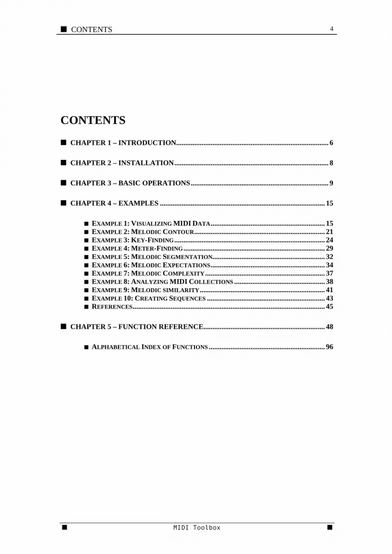
CONTENTS
■ CHAPTER 1 – INTRODUCTION.................................................................................... 6
■ CHAPTER 2 – INSTALLATION..................................................................................... 8
■ CHAPTER 3 – BASIC OPERATIONS............................................................................ 9
■ CHAPTER 4 – EXAMPLES ........................................................................................... 15
■ EXAMPLE 1: VISUALIZING MIDI DATA............................................................... 15 ■ EXAMPLE 2: MELODIC CONTOUR........................................................................ 21 ■ EXAMPLE 3: KEY-FINDING................................................................................... 24 ■ EXAMPLE 4: METER-FINDING.............................................................................. 29 ■ EXAMPLE 5: MELODIC SEGMENTATION.............................................................. 32 ■ EXAMPLE 6: MELODIC EXPECTATIONS............................................................... 34 ■ EXAMPLE 7: MELODIC COMPLEXITY.................................................................. 37 ■ EXAMPLE 8: ANALYZING MIDI COLLECTIONS .................................................. 38 ■ EXAMPLE 9: MELODIC SIMILARITY..................................................................... 41 ■ EXAMPLE 10: CREATING SEQUENCES ................................................................. 43 ■ REFERENCES.......................................................................................................... 45
■ CHAPTER 5 – FUNCTION REFERENCE................................................................... 48
■ ALPHABETICAL INDEX OF FUNCTIONS ................................................................ 96

■ CHAPTER 1 – INTRODUCTION 6
■ MIDI Toolbox ■
CHAPTER 1 – INTRODUCTION MIDI Toolbox provides a set of Matlab functions, which together have all the necessary machinery to analyze and visualize MIDI data. The development of the Toolbox has been part of ongoing research involved in topics relating to musical data-mining, modelling music perception and decomposing the data for and from perceptual experiments. Although MIDI data is not necessarily a good representation of music in general, it suffices for many research questions dealing with concepts such as melodic contour, tonality and pulse finding. These concepts are intriguing from the point of view of music perception and the chosen representation greatly affects the way these issues can be approached. MIDI is not able to handle the timbre of music and therefore it unsuitable representation for a number of research questions (for summary, see Hewlett and Selfridge-Field, 1993-94, p. 11-28). All musical signals may be processed from acoustic representation and there are suitable tools available for these purposes (e.g. IPEM toolbox, Leman et al., 2000). However, there is a body of essential questions of music cognition that benefit from a MIDI-based approach. MIDI does not contain notational information, such as phrase and bar markings, and neither is that information conveyed in explicit terms to the ears of music listeners. Consequently, models of music cognition must infer these musical cues from the pitch, timing and velocity information that MIDI provides. Another advantage of the MIDI format is that it is extremely wide-spread among the research community as well as having a wider group of users amongst the music professionals, artists and amateur musicians. MIDI is a common file format between many notation, sequencing and performance programs across a variety of operating systems. Numerous pieces of hardware exist that collect data from musical performances, either directly from the instrument (e.g. digital pianos and other MIDI instruments) or from the movements of the artists (e.g. motion tracking of musician’s gestures, hand movements etc.). The vast majority of this technology is based on MIDI representation. However, the analysis of the MIDI data is often developed from scratch for each research question. The aim of MIDI Toolbox is to provide the core representation and functions that are needed most often. These basic tools are designed to be modular to allow easy further development and tailoring for specific analysis needs. Another aim is to facilitate efficient use and to lower the “threshold of practicalities”. For example, the Toolbox can be used as teaching aid in music cognition courses. This documentation provides a description of the Toolbox (Chapter 1), installation and system requirements (Chapter 2). Basic issues are explained in Chapter 3. Chapter 4 demonstrates the Toolbox functions using various examples. The User’s Guide does not describe any of the underlying theories in detail. Chapter 5 focuses on a collection format and Chapter 6 is the reference section, describing all functions in the Toolbox. The online reference documentation provides direct hypertext links to specific Toolbox functions. This is available at http://www.jyu.fi/musica/miditoolbox/
7 CHAPTER 1 – INTRODUCTION ■
■ MIDI Toolbox ■
This User’s Guide assumes that the readers are familiar with Matlab. At the moment, the MIDI Toolbox is a collection of Matlab functions that do not require any extra toolboxes to run. Signal processing and Statistics toolboxes – both available separately from Mathworks – offer useful extra tools for the analysis of perceptual experiments. MIDI Toolbox comes with no warranty. This is free software, and you are welcome to redistribute it under certain conditions. See License.txt for details of GNU General Public License. We would like to thank various people contributing to the toolbox. The conversion to and from MIDI file is based on the C source code by Piet van Oostrum, which, in turn, uses the midifile library written by Tim Thompson and updated by Michael Czeiszperger. Brian Cameron found out some sneaky bugs in the aforementioned C source code. Micah Bregman helped to check parts of the manual and wrote out some new functions.
Comments, suggestions or questions? Many functions are still not completely tested in MIDI Toolbox version 1.0. Check the online forum for corrections and revisions: http://www.jyu.fi/musica/miditoolbox/forum.html Alternatively, you can report any bugs or problems to: Tuomas Eerola, Petri Toiviainen {ptee, ptoiviai}@cc.jyu.fi Department of Music University of Jyväskylä P.O. BOX 35 40014 University of Jyväskylä Finland

■ CHAPTER 1 – INTRODUCTION 8
■ MIDI Toolbox ■
CHAPTER 2 – INSTALLATION Availability The whole toolbox is available either as a zipped package from the internet (http://www.jyu.fi/musica/miditoolbox/).
Installation Unpack the MIDI Toolbox file package you have downloaded. For this, use a program like Winzip for Windows and Stuffit Expander for Macintosh. This will create a directory called miditoolbox. Secondly, a version of the Matlab program needs to be installed (see www.mathworks.com). Thirdly, the Toolbox needs to be defined in the Matlab path variable.
Windows (98, 2000, XP) The MIDI Toolbox version 1.0 is compatible with Matlab 5.3 and Matlab 6.5.
Macintosh (OS X) The MIDI Toolbox version 1.0 is compatible with Matlab 6.5 for Macintosh.
Linux Currently not tested but should be compatible.
9 CHAPTER 3 – BASIC OPERATIONS ■
■ MIDI Toolbox ■
CHAPTER 3 – BASIC OPERATIONS
Basic issues In this tutorial, we assume that the reader has basic knowledge of the Matlab command syntax. Many good tutorials exist in the Internet, see: http://www.math.ufl.edu/help/matlab-tutorial/ http://www.math.mtu.edu/~msgocken/intro/intro.html http://www.helsinki.fi/~mjlaine/matlab/index.html (in Finnish) http://www.csc.fi/oppaat/matlab/matlabohje.pdf (in Finnish) In the following examples, the commands that are typed to Matlab command prompt are written in monospaced font and are preceded by the » sign. Help is also available within the Matlab session. For example, to understand what a particular function does, type help and the name of the function at the command prompt. For example, to obtain information about how the pitch-class distribution function works, type: » help pcdist1 To see a list of all available functions in the Toolbox, type: » help miditoolbox
Reading MIDI files into Matlab The basic functions in MIDI Toolbox read and manipulate type 0 and type 1 MIDI files. The following command reads and parses a MIDI file called laksin.mid and stores it as a matrix of notes called nmat in Matlab’s workspace: » nmat = readmidi('laksin.mid'); This particular MIDI file contains the first two verses of a Finnish Folk song called "Läksin minä kesäyönä" (trad.).
Basic terms Notematrix (or nmat) refers to a matrix representation of note events in a MIDI file. We can now type nmat and see what the notematrix of the folk song looks like.
■ CHAPTER 3 – BASIC OPERATIONS 10
■ MIDI Toolbox ■
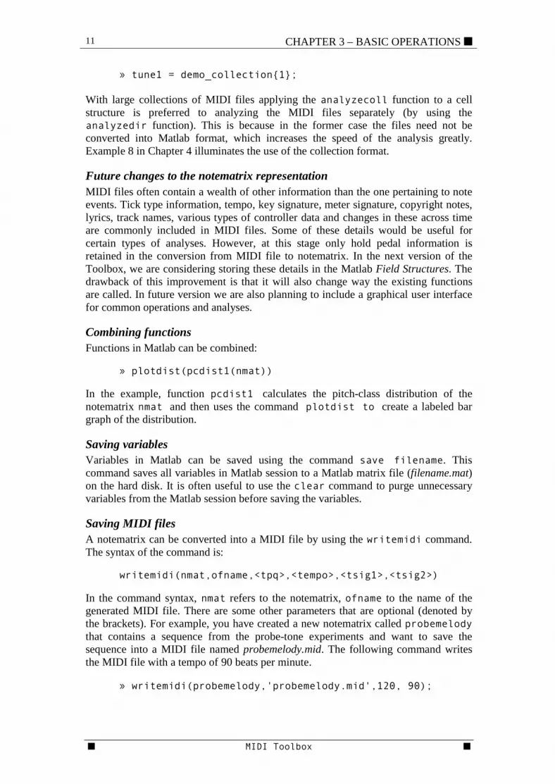
» nmat nmat = 0 0.9000 1.0000 64.0000 82.0000 0 0.5510 1.0000 0.9000 1.0000 71.0000 89.0000 0.6122 0.5510 2.0000 0.4500 1.0000 71.0000 82.0000 1.2245 0.2755 2.5000 0.4500 1.0000 69.0000 70.0000 1.5306 0.2755 3.0000 0.4528 1.0000 67.0000 72.0000 1.8367 0.2772 3.5000 0.4528 1.0000 66.0000 72.0000 2.1429 0.2772 4.0000 0.9000 1.0000 64.0000 70.0000 2.4490 0.5510 5.0000 0.9000 1.0000 66.0000 79.0000 3.0612 0.5510 6.0000 0.9000 1.0000 67.0000 85.0000 3.6735 0.5510 7.0000 1.7500 1.0000 66.0000 72.0000 4.2857 1.0714 We see that the variable nmat contains a 7 x 10 matrix filled with numbers. The columns refer to various types of information such as MIDI pitch and MIDI channel. The rows stand for the individual note events (in this case, the melody has 10 notes and each of them is described in terms pitch, onset time, duration, volume and so forth). The labels of the columns are as follows: ONSET DURATION MIDI MIDI VELOCITY ONSET DURATION (BEATS) (BEATS) channel PITCH (SEC) (SEC) The first column indicates the onset of the notes in beats (based on ticks per quarter note) and the second column the duration of the notes in these same beat-values. The third column denotes the MIDI channel (1-16), and the fourth the MIDI pitch, where middle C (C4) is 60. The fifth column is the velocity describing how fast the key of the note is pressed, in other words, how loud the note is played (0-127). The last two columns correspond to the first two (onset in beats, duration in beats) except that seconds are used instead of beats. Often one wants to refer only to pitch or duration values in the notematrix. For clarity and convenience, these columns may be called by few basic selector functions that refer to each specific column only. These are onset (either 'beat' or 'sec', the former is the default), dur (either 'beat' or 'sec'), channel, pitch, and velocity. For example, pitch(nmat) returns only the MIDI notes values of the notematrix and onset(nmat) returns only the onset times (in beats) of the events in the notematrix.
Collection format Large corpora of music are more convenient to process in Matlab if they are stored in Matlab’s own cell structures rather than keeping them as MIDI files that are loaded separately for the analysis. You can store multiple notematrices in cell structures from a directory of MIDI files by using dir2cellmatr function. The function processes all MIDI files in the current directory and stores the notematrices and the filenames in the variables of your choice: » [demo_collection,filenames] = dir2cellmatr; After creating cell matrix structure of the MIDI files, individual notematrices can be called by the following convention:
11 CHAPTER 3 – BASIC OPERATIONS ■
■ MIDI Toolbox ■
» tune1 = demo_collection{1}; With large collections of MIDI files applying the analyzecoll function to a cell structure is preferred to analyzing the MIDI files separately (by using the analyzedir function). This is because in the former case the files need not be converted into Matlab format, which increases the speed of the analysis greatly. Example 8 in Chapter 4 illuminates the use of the collection format.
Future changes to the notematrix representation MIDI files often contain a wealth of other information than the one pertaining to note events. Tick type information, tempo, key signature, meter signature, copyright notes, lyrics, track names, various types of controller data and changes in these across time are commonly included in MIDI files. Some of these details would be useful for certain types of analyses. However, at this stage only hold pedal information is retained in the conversion from MIDI file to notematrix. In the next version of the Toolbox, we are considering storing these details in the Matlab Field Structures. The drawback of this improvement is that it will also change way the existing functions are called. In future version we are also planning to include a graphical user interface for common operations and analyses.
Combining functions Functions in Matlab can be combined: » plotdist(pcdist1(nmat)) In the example, function pcdist1 calculates the pitch-class distribution of the notematrix nmat and then uses the command plotdist to create a labeled bar graph of the distribution.
Saving variables Variables in Matlab can be saved using the command save filename. This command saves all variables in Matlab session to a Matlab matrix file (filename.mat) on the hard disk. It is often useful to use the clear command to purge unnecessary variables from the Matlab session before saving the variables.
Saving MIDI files A notematrix can be converted into a MIDI file by using the writemidi command. The syntax of the command is: writemidi(nmat,ofname,<tpq>,<tempo>,<tsig1>,<tsig2>) In the command syntax, nmat refers to the notematrix, ofname to the name of the generated MIDI file. There are some other parameters that are optional (denoted by the brackets). For example, you have created a new notematrix called probemelody that contains a sequence from the probe-tone experiments and want to save the sequence into a MIDI file named probemelody.mid. The following command writes the MIDI file with a tempo of 90 beats per minute. » writemidi(probemelody,'probemelody.mid',120, 90);
■ CHAPTER 3 – BASIC OPERATIONS 12
■ MIDI Toolbox ■
Playing notematrices There are two methods of listening to the contents of a notematrix. The first method involves playing the MIDI file created by nmat2mf command using the internal MIDI player of the operating system (such as Quicktime, Mediaplayer or Winamp). This method uses the following command: » playmidi(nmat) This function is dependent on the operating system. In Windows, use definemidiplayer function and choose a midi player of your choice by browsing and selecting the correct executable from your hard disk (Media Player, Winamp, etc). This function writes the path and the filename down to midiplayer.txt in MIDI Toolbox directory for future use. In MacOS X, the path is already predefined in the abovementioned files. The second method is to synthesize the notematrix into waveform using nmat2snd function. This is computationally more demanding, especially if the notematrix is large. Matlab can render these results into audible form by using sound or soundsc function or alternatively the waveform may be written into a file using wavwrite function. Simple way to hear the notematrix is type: » playsound(nmat);
Referring to parts of a notematrix Often one wants to select only a certain part of a notematrix for analysis. For example, instead of analyzing the whole MIDI sequence, you may wish to examine the first 8 bars or select only MIDI events in a certain MIDI channel. Basic selection is accomplished using Matlab’s own index system, for example: » first_12_notes = laksin(1:12,:); It is also possible to refer to MIDI Toolbox definitions and functions when selecting parts of the notematrix. The following examples give a few ideas of how these may be used. Many of these functions belong to the filter category (see Chapter 6). » first_4_secs = onsetwindow(laksin,0,4,'sec'); » first_meas = onsetwindow(laksin,0,3,'beat'); » between_1_and_2_sec = onsetwindow(laksin,1,2,'sec'); » only_in_channel1 = getmidich(laksin,1); » remove_channel10 = dropmidich(laksin,10); » no_short_notes = dropshortnotes(laksin,'sec',0.3)
Manipulating note matrices Often one wants to find and manipulate the tempo of a notematrix. Here’s an example of how the tempo is obtained and then set to a faster rate.
13 CHAPTER 3 – BASIC OPERATIONS ■
■ MIDI Toolbox ■
» tempo = gettempo(laksin) » tempo = 98.000 » laksin_128bpm = settempo(laksin,128); To scale any values in the notematrix, use scale command: » laksin_with_halved_durations = scale(laksin,'dur',0.5); One can assign any parameter (channel, duration, onset, velocity, pitch) in the notematrix a certain fixed value. For instance, to set all note velocities to 64, setvalues command may be used: » laksin_velocity64 = setvalues(laksin,'vel',64); Transposing the MIDI file is also a useful operation. This example transposes the folk tune Läksin a major third down (minus four semitones). » laksin_in_c = shift(laksin,'pitch',-4); Transposition can also be done to a velocity or channel information of the notematrix. Here’s an example of channel alteration. » laksin_channel2 = shift(laksin,'chan',1); If you do not know the key of the MIDI file and wish to transpose the file to a C major or C minor key, it can be performed using the transpose2c function. This method draws on a built-in key-finding algorithm, which is described later. » laksin_in_c = transpose2c(laksin); It is also possible to combine different notematrices using Matlab’s regular command syntax. To create Finnish folk tune Läksin in parallel thirds, use: » laksin_parallel_thirds = [laksin; laksin_in_c]; Sometimes a notematrix might need to be quantized. This is relatively easy to carry out using quantize function. In this example, a Bach prelude is quantized using sixteenth beat resolution. The first argument quantizes the onsets, the second argument the durations and the third argument filters out notes that are shorter than the criteria (sixteenth notes in this case): » prelude_edited = quantize(prelude, 1/16,1/16,1/16); In many cases one wishes to eliminate certain aspects of the notematrix. For example, a simple way to get the upper line of the polyphonic notematrix is to use extreme function: » prelude_edited = extreme(prelude_edited,'high'); Also, leading silence in notematrix is something that often is unnecessary. This can be removed using the trim function:

■ CHAPTER 3 – BASIC OPERATIONS 14
■ MIDI Toolbox ■
» prelude_edited = trim(prelude_edited);
Demonstrations Demonstrations, which are loosely based on the examples described in the next chapter, are available in the MIDI Toolbox directory. Type in mididemo to go through the demos.

15 CHAPTER 4 – EXAMPLES ■
■ MIDI Toolbox ■
CHAPTER 4 – EXAMPLES Example 1: Visualizing MIDI Data
The pianoroll function displays conventional pianoroll notation as it is available in sequencers. The function has the following syntax: pianoroll(nmat,<varargin>); The first argument refers to the notematrix and other arguments are optional. Possible arguments refer to axis labels (either MIDI note numbers or note names for Y-axis and either beats or seconds for the X-axis), colors or other options. For example, the following command outputs the pitch and velocity information: » pianoroll(laksin,'name','sec','vel');
Figure 1: Pianoroll notation of the two first phrases of Läksin minä kesäyönä. The lower panel shows the velocity information.
Figure 2. Notation of first two verses of the Finnish Folk tune "Läksin minä kesäyönä".
0 1 2 3 4 5 6 7 8 9 10C4#D4 D4#E4 F4 F4#G4 G4#A4 A4#B4 C5 C5#
Time in seconds
Pitc
h
0 1 2 3 4 5 6 7 8 9 100
20
4060
80100
120
Time in seconds
Velo
city
■ CHAPTER 4 – EXAMPLES 16
■ MIDI Toolbox ■
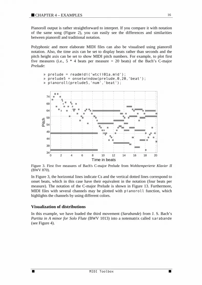
Pianoroll output is rather straightforward to interpret. If you compare it with notation of the same song (Figure 2), you can easily see the differences and similarities between pianoroll and traditional notation. Polyphonic and more elaborate MIDI files can also be visualised using pianoroll notation. Also, the time axis can be set to display beats rather than seconds and the pitch height axis can be set to show MIDI pitch numbers. For example, to plot first five measures (i.e., 5 * 4 beats per measure = 20 beats) of the Bach’s C-major Prelude: » prelude = readmidi('wtcii01a.mid'); » prelude5 = onsetwindow(prelude,0,20,'beat'); » pianoroll(prelude5,'num','beat');
Figure 3. First five measures of Bach's C-major Prelude from Wohltemperierte Klavier II (BWV 870).
In Figure 3, the horizontal lines indicate Cs and the vertical dotted lines correspond to onset beats, which in this case have their equivalent in the notation (four beats per measure). The notation of the C-major Prelude is shown in Figure 13. Furthermore, MIDI files with several channels may be plotted with pianoroll function, which highlights the channels by using different colors.
Visualization of distributions In this example, we have loaded the third movement (Sarabande) from J. S. Bach’s Partita in A minor for Solo Flute (BWV 1013) into a notematrix called sarabande (see Figure 4).
0 2 4 6 8 10 12 14 16 18 2034
39
44
49
54
59
64
69
74
Time in beats
Pitc
h

17 CHAPTER 4 – EXAMPLES ■
■ MIDI Toolbox ■
Figure 4. Bach's Flute Sarabande (BWV 1013).
First, we can examine the note distribution of the Sarabande in order to see whether the key signature is apparent from the distribution of the pitch-classes. The following command creates a bar chart of the pitch-class distribution of the Sarabande. » plotdist(pcdist1(sarabande));
Figure 5. Pitch-class distribution in Bach's Flute Sarabande (BWV 1013).
C C# D D# E F F# G G# A A# B0
0.02
0.04
0.06
0.08
0.1
0.12
0.14
0.16
0.18
Pitch-class
Pro
porti
on (%
)

■ CHAPTER 4 – EXAMPLES 18
■ MIDI Toolbox ■
The inner function, pcdist1, calculates the proportion of each pitch-class in the sequence, and the outer function, plotdist, creates the labeled graph. From the resulting graph, shown in Figure 5, we can infer that the Sarabande is indeed in A minor key as A, C and E are the most commonly used tones. More about inferring the key in a separate section on key-finding (Example 3). Another basic description of musical content is the interval structure. In monophonic music this is easily compiled, as shown below, but detecting successive intervals in polyphonic music is a difficult perceptual task and will not be covered here. To see what kind of intervals are most common in the Sarabande, type: » plotdist(ivdist1(sarabande));
Figure 6. Interval distribution in Bach's Flute Sarabande (BWV 1013).
In the middle, P1 stands for unison (perfect first), i.e. note repetitions, which are fairly rare in this work (P8 stands for perfect octave, m3 is the minor third, M3 is a major third and so on). Let us compare the distribution of interval sizes and direction to the results obtained from analysis of large musical corpora by Vos and Troost (1989). To obtain suitable distributions of Sarabande, we use function ivdirdist1 and ivsizedist1 (see Figure 7).
-P8 -M6 -d5 -m3 P1 +m3 +d5 +M6 +P80
0.05
0.1
0.15
0.2
0.25
Interval
Prop
ortio
n (%
)

19 CHAPTER 4 – EXAMPLES ■
■ MIDI Toolbox ■
Pro
porti
on a
scen
ding
(%)
MI2 MA2 MI3 MA3 P4 D5 P5 MI6 MA6 MI7 MA7 P80
0.1
0.2
0.3
0.4
0.5
0.6
0.7
0.8
0.9
1
Pro
porti
on a
scen
ding
(%)
MI2 MA2 MI3 MA3 P4 D5 P5 MI6 MA6 MI7 MA7 P80
0.1
0.2
0.3
0.4
0.5
0.6
0.7
0.8
0.9
1
MI2 MA2 MI3 MA3 P4 D5 P50
0.05
0.1
0.15
0.2
0.25
Pro
porti
on o
f occ
urre
nce
Interval
P1 MI2MA2MI3MA3 P4 D5 P5 MI6MA6MI7MA7 P80
0.05
0.1
0.15
0.2
0.25
0.3
0.35
Pro
porti
on (%
)
Figure 7. The top left panel shows the distribution of interval sizes in Sarabande and the lower left panels displays the theoretical frequency of occurrence of intervals according to Dowling and Harwood (1986). The top right panels shows the proportion of the ascending intervals and the lower right panel displays the same data in collection of folk music (N=327), compiled by Vos and Troost (1989).
We see in Figure 7 that in the corpus analyzed by Vos and Troost (1989) the interval structure is usually asymmetric (lower right panel). This means that large intervals tend to ascend whereas small intervals tend to descend. This is not evident in Sarabande (panels on the right) as the fifths tend to descend rather than ascend. Displaying the distributions of two-tone continuations in Sarabande is similar to displaying tone distributions: » plotdist(pcdist2(sarabande));
Distributions in Sarabande
Theoretical distribution Distribution in folk music

■ CHAPTER 4 – EXAMPLES 20
■ MIDI Toolbox ■
Figure 8. The proportion of two-note continuations in Bach's Flute Sarabande (BWV 1013). The colorbar at the right displays the proportion associated with each colour.
Figure 8 shows the proportion of tone transitions in Sarabande. The most common transition is from dominant (E) to D and next most common transition is the F to dominant E. Commonly, the diagonal of the tone transition matrix shows high proportion of occurrences but this work clearly avoids unisons. The few unisons shown in the transition matrix are due to octave displacement. Note that these statistics are different from the interval distributions. It is also possible to view a distribution of note durations in a similar manner (functions durdist1 and durdist2). In Matlab, there are further visualization techniques that can be used to display the distributions. Quite often, plotting the data using different colors is especially informative. In some cases, three-dimensional plots can aid the interpretation of the data (see Example 7 for a three-dimensional version of note transitions.).
0
0.01
0.02
0.03
0.04
0.05
0.06
0.07
0.08
0.09
0.1
Pitch-class 2
Pitc
h-cl
ass
1
C C# D D# E F F# G G# A A# BC
C#
D
D#
E
F
F#
G
G#
A
A#
B
21 CHAPTER 4 – EXAMPLES ■
■ MIDI Toolbox ■
Example 2: Melodic Contour
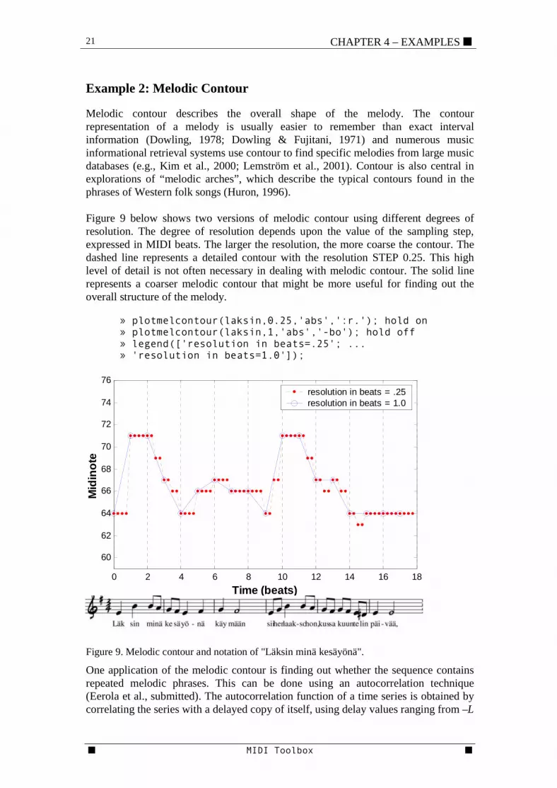
Melodic contour describes the overall shape of the melody. The contour representation of a melody is usually easier to remember than exact interval information (Dowling, 1978; Dowling & Fujitani, 1971) and numerous music informational retrieval systems use contour to find specific melodies from large music databases (e.g., Kim et al., 2000; Lemström et al., 2001). Contour is also central in explorations of “melodic arches”, which describe the typical contours found in the phrases of Western folk songs (Huron, 1996). Figure 9 below shows two versions of melodic contour using different degrees of resolution. The degree of resolution depends upon the value of the sampling step, expressed in MIDI beats. The larger the resolution, the more coarse the contour. The dashed line represents a detailed contour with the resolution STEP 0.25. This high level of detail is not often necessary in dealing with melodic contour. The solid line represents a coarser melodic contour that might be more useful for finding out the overall structure of the melody. » plotmelcontour(laksin,0.25,'abs',':r.'); hold on » plotmelcontour(laksin,1,'abs','-bo'); hold off » legend(['resolution in beats=.25'; ... » 'resolution in beats=1.0']);
Figure 9. Melodic contour and notation of "Läksin minä kesäyönä".
One application of the melodic contour is finding out whether the sequence contains repeated melodic phrases. This can be done using an autocorrelation technique (Eerola et al., submitted). The autocorrelation function of a time series is obtained by correlating the series with a delayed copy of itself, using delay values ranging from –L
0 2 4 6 8 10 12 14 16 18
60
62
64
66
68
70
72
74
76
Time (beats)
Mid
inot
e
resolution in beats = .25resolution in beats = 1.0

■ CHAPTER 4 – EXAMPLES 22
■ MIDI Toolbox ■
to +L, where L denotes the total length of the time series. A time series is autocorrelated if it is possible to predict its value at a given point of time by knowing its value at other points of time. Positive autocorrelation means that points at a certain distance away from each other have similar values (Box, Jenkins & Reinsel, 1994). » l = reftune('laksin'); » c = melcontouracorr(l); » t = [-(length(c)-1)/2:1:(length(c)-1)/2]*.1; » plot(t,c,'k');md = round(max(onset(l))+ dur(l(end,:))); » axis([-md md -0.4 1]); xlabel('\bfLag (in beats)') » set(gca,'XTick',-md:2:md); ylabel('\bfCorr. coeff.')
Figure 10. A plot of autocorrelation across melodic contour of "Läksin minä kesäyönä".
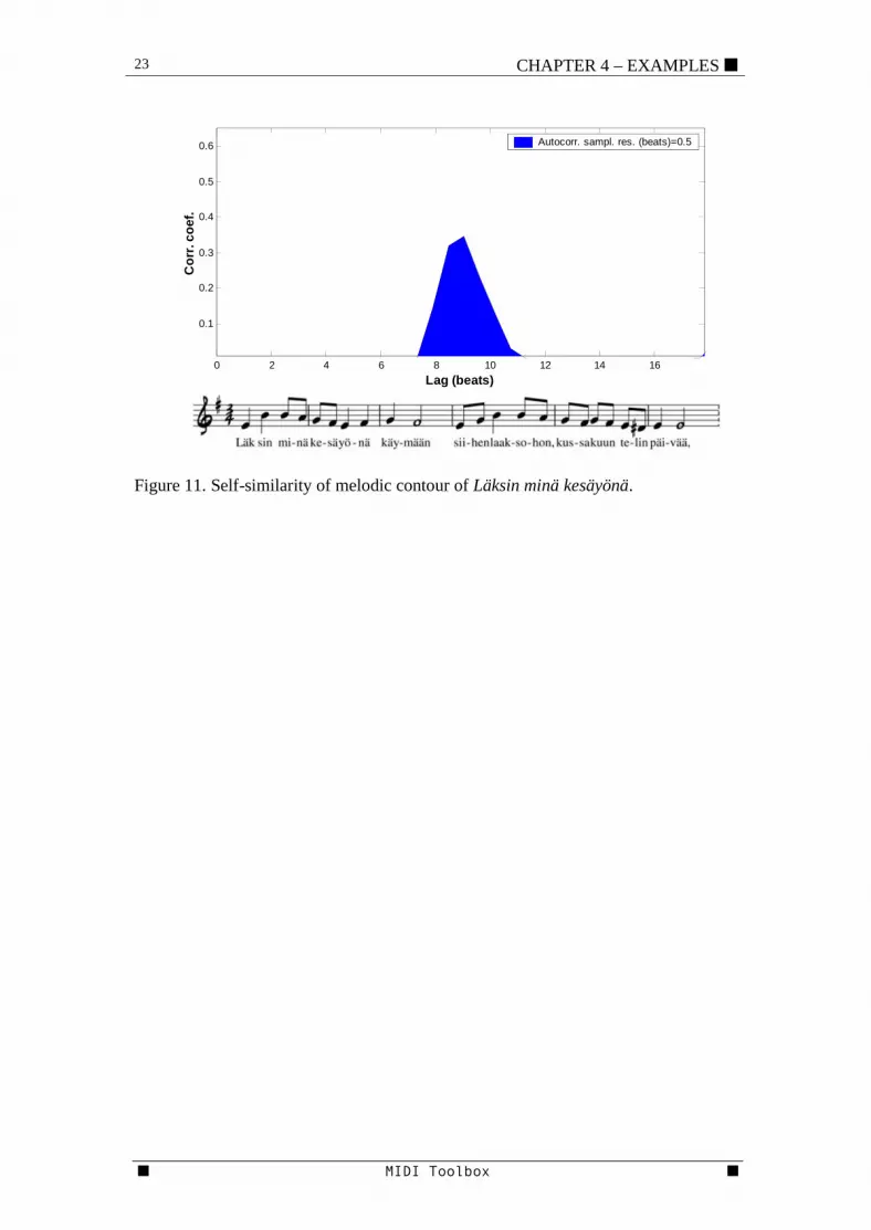
Figure 10 shows the autocorrelation function of the contour of Läksin mina kesäyönä. At the middle of the figure (at the peak, lag 0 beats) the autocorrelation function gives the result of 1.0, perfect correlation, because at this point the melodic contour is compared with itself. The autocorrelation function is always symmetric with respect to the point corresponding to zero lag. Therefore, only the right halve needs to be regarded to estimate the degree of self-similarity. The shaded area shows the self-similarity of the melodic contour; only the positive correlations of the autocorrelation function (half-wave rectification) are observed. This relevant, right portion of the autocorrelation function may be plotted using the 'ac' parameter in melcontour command: » plotmelcontour(l,0.5,'abs','b','ac');
-18 -16 -14 -12 -10 -8 -6 -4 -2 0 2 4 6 8 10 12 14 16 18-0.4
-0.2
0
0.2
0.4
0.6
0.8
1
Lag (in beats)
Corr
. coe
ff.
23 CHAPTER 4 – EXAMPLES ■
■ MIDI Toolbox ■
Figure 11. Self-similarity of melodic contour of Läksin minä kesäyönä.
0 2 4 6 8 10 12 14 16
0.1
0.2
0.3
0.4
0.5
0.6
Lag (beats)
Cor
r. co
ef.
Autocorr. sampl. res. (beats)=0.5

■ CHAPTER 4 – EXAMPLES 24
■ MIDI Toolbox ■
Example 3: Key-Finding
The classic Krumhansl & Schmuckler key-finding algorithm (Krumhansl, 1990), is based on key profiles obtained from empirical work by Krumhansl & Kessler (1982). The key profiles were obtained in a series of experiments, where listeners heard a context sequence, consisting of an incomplete major or minor scale or a chord cadence, followed by each of the chromatic scale pitches in separate trials. (See Example 9 for instructions on creating the probe-tone stimuli using the Toolbox). Figure 12 shows the averaged data from all keys and contexts, called C major and C minor key profiles.
Figure 12. Probe-tone ratings for the keys of C major and C minor (Krumhansl & Kessler, 1982).
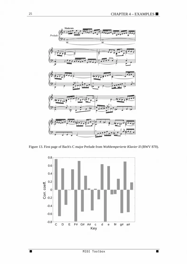
In the K-S key-finding algorithm, the 24 individual key profiles, 12 major and 12 minor key profiles, are correlated with the pitch-class distribution of the piece weighted according to their duration. This gives a measure of the strength of each key. Let us take the C major Prelude in J. S. Bach's Wohltemperierte Klavier II (BWV 870). The first page of this Prelude is shown in Figure 13 . We load this file into a variable called prelude and take only the first 10 measures (first page in Figure 13) of it to find a likely key area: » prelude10=onsetwindow(prelude,0,40); » keyname(kkkey(prelude10)) » ans = 'C' The inner function in the second command line (kkkey) performs the K-S key-finding algorithm and the outer function changes the numerical output of the inner function to a letter denoting the key. Not surprisingly, the highest correlation of the note distribution in the first 10 measures of the Prelude is obtained with the C major key profile. A closer look at the other candidates the algorithm offers reveals the strength of all keys: » keystrengths = kkcc(prelude10); % corr. to all keys » plotdist(keystrengths); % plot all corr. coefficients Figure 15 displays the correlation coefficient to all 24 key profiles. According to the figure, G major and a minor keys are also high candidates for the most likely key. This is not surprising considering that these are dominant and parallel minor keys to C major.
C C# D D# E F F# G G# A A# B1
2
3
4
5
6
7
Pro
be-to
ne ra
ting
C major
C C# D D# E F F# G G# A A# B1
2
3
4
5
6
7
Pro
be-to
ne ra
ting
C minor
25 CHAPTER 4 – EXAMPLES ■
■ MIDI Toolbox ■
Figure 13. First page of Bach's C major Prelude from Wohltemperierte Klavier II (BWV 870).
C D E F# G# A# c d e f# g# a#-0.8
-0.6
-0.4
-0.2
0
0.2
0.4
0.6
0.8
Key
Cor
r. co
eff.

■ CHAPTER 4 – EXAMPLES 26
■ MIDI Toolbox ■
Figure 14. Correlation coefficients of the pitch-class distribution in Bach's C-major prelude to all 24 key profiles.
Another way of exploring key-finding is to look at how tonality changes over time. In the technique, key-finding is performed within a small window that runs across the length of the music. This operation uses the movewindow function. Below is an example of finding the maximal key correlation using a 4-beat window that is moved by 2 beats at a time. » prelude4=onsetwindow(prelude,0,16,'beat'); » keys = movewindow(prelude4,4,2,'beat','maxkkcc'); » label=keyname(movewindow(prelude4,4,2,'beat','kkkey')); » time=0:2:16; plot(time,keys,':ko','LineWidth',1.25); » axis([-0.2 16.2 .4 1]) » for i=1:length(label) » text(time(i),keys(i)+.025,label(i),... » 'HorizontalAlignment','center','FontSize',12); » end » ylabel('\bfMax. key corr. coeff.'); » xlabel('\bfTime (beats)')
Figure 15. Maximum key correlation coefficients across time in the beginning of the C-major Prelude.
Figure 15 displays the key changes over time, showing the movement towards the F major (meas. 4) and further to G major (meas. 6). Although the measure shows the strength of the key correlation, it gives a rather simplistic view of the tonality as the dispersion of the key center between the alternate local keys is not shown. A recent dynamic model of tonality induction (Toiviainen & Krumhansl, 2003) calculates local tonality based on key profiles. The results may be projected onto a self-organizing map (SOM) trained with the 24 key profiles. In the following example, the function calculates the key strengths and creates the projection. The second argument in the syntax example defines the colorbar and the third the color. » keysom(prelude10,1); % create a color figure
0 2 4 6 8 10 12 14 160.4
0.5
0.6
0.7
0.8
0.9
1
c
CC F
e
e
a
d d
Max
. key
cor
r. co
eff.
Time (beats)

27 CHAPTER 4 – EXAMPLES ■
■ MIDI Toolbox ■
Figure 16. Self-organizing map (SOM) of the tonality in Bach’s C-major Prelude.
The map underlying the tonal strengths in Figure 16 is toroid in shape, which means that the opposite edges are attached to each other. The local tonality is the strongest in the area between a minor and C major. This visualization of tonality can be used to show the fluctuations of the key center and key strength over time. Below is an example of this using a 4-beat window that steps 2 beats forward each time. » keysomanim(prelude4,4,2); % show animation in Matlab » keysomanim(prelude4,4,2,'beat','strip'); % show strips
Beat 2.0
C
Db
D
Eb
E
F
Gb
G
Ab
A
Bb
B
c
c#
d
d#
e
f
f#
g
ab
a
bb
b
Beat 4.0
C
Db
D
Eb
E
F
Gb
G
Ab
A
Bb
B
c
c#
d
d#
e
f
f#
g
ab
a
bb
b
Beat 6.0
C
Db
D
Eb
E
F
Gb
G
Ab
A
Bb
B
c
c#
d
d#
e
f
f#
g
ab
a
bb
b
Beat 8.0
C
Db
D
Eb
E
F
Gb
G
Ab
A
Bb
B
c
c#
d
d#
e
f
f#
g
ab
a
bb
b
Beat 10.0
C
Db
D
Eb
E
F
Gb
G
Ab
A
Bb
B
c
c#
d
d#
e
f
f#
g
ab
a
bb
b
Beat 12.0
C
Db
D
Eb
E
F
Gb
G
Ab
A
Bb
B
c
c#
d
d#
e
f
f#
g
ab
a
bb
b
Beat 14.0
C
Db
D
Eb
E
F
Gb
G
Ab
A
Bb
B
c
c#
d
d#
e
f
f#
g
ab
a
bb
b
Beat 16.0
C
Db
D
Eb
E
F
Gb
G
Ab
A
Bb
B
c
c#
d
d#
e
f
f#
g
ab
a
bb
b
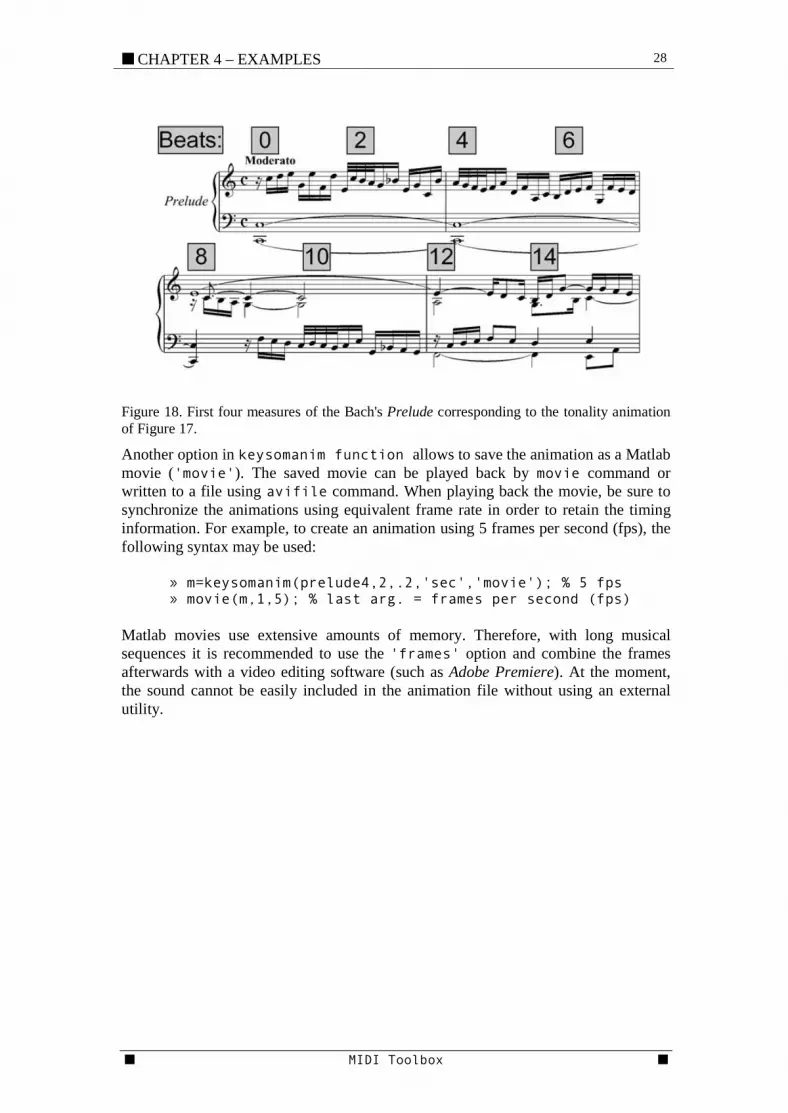
Figure 17. First four measures (two frames per measure) of the tonality animation in Bach's Prelude.
Figure 17 displays the tonality of the first four measures of the Prelude. From the separate figures one can see how the tonal center is first firmly in C major and then it moves towards other regions, F, e, etc.
■ CHAPTER 4 – EXAMPLES 28
■ MIDI Toolbox ■
Figure 18. First four measures of the Bach's Prelude corresponding to the tonality animation of Figure 17.
Another option in keysomanim function allows to save the animation as a Matlab movie ('movie'). The saved movie can be played back by movie command or written to a file using avifile command. When playing back the movie, be sure to synchronize the animations using equivalent frame rate in order to retain the timing information. For example, to create an animation using 5 frames per second (fps), the following syntax may be used: » m=keysomanim(prelude4,2,.2,'sec','movie'); % 5 fps » movie(m,1,5); % last arg. = frames per second (fps) Matlab movies use extensive amounts of memory. Therefore, with long musical sequences it is recommended to use the 'frames' option and combine the frames afterwards with a video editing software (such as Adobe Premiere). At the moment, the sound cannot be easily included in the animation file without using an external utility.
29 CHAPTER 4 – EXAMPLES ■
■ MIDI Toolbox ■
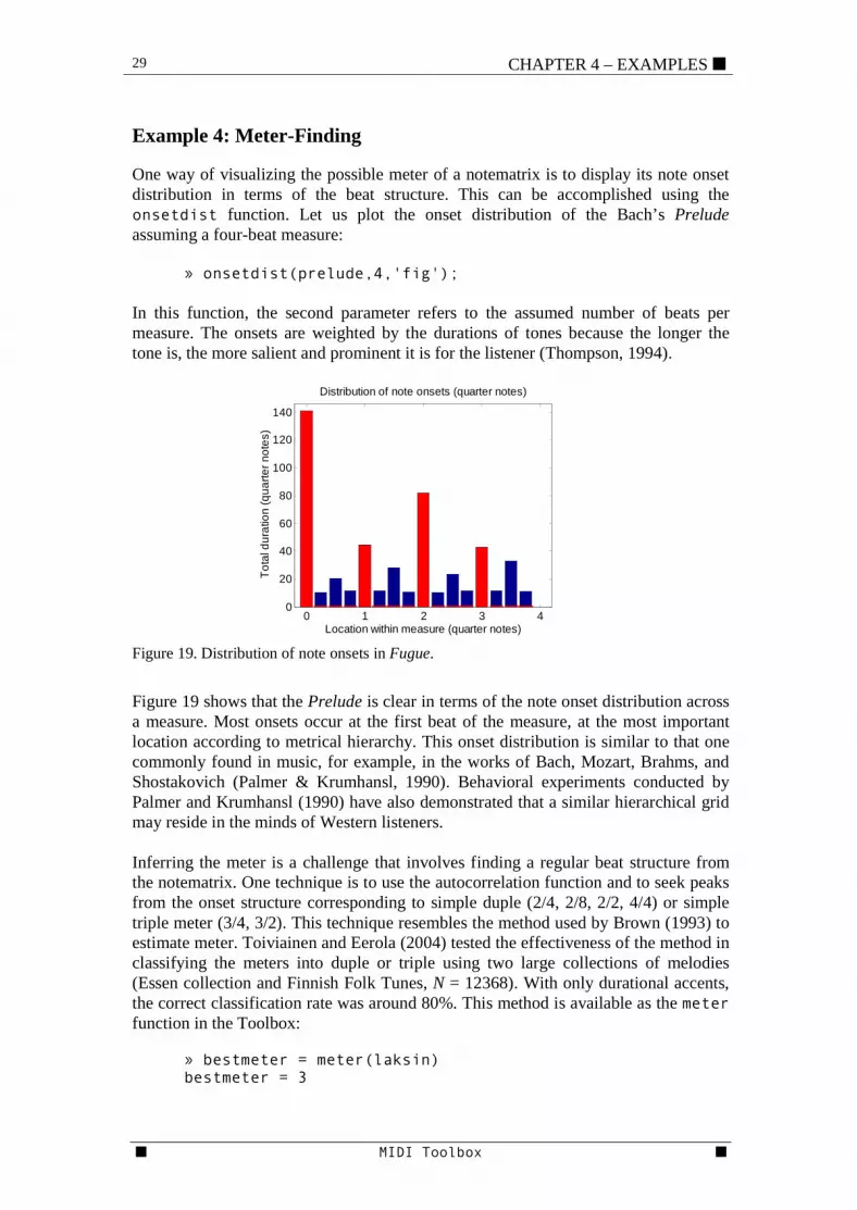
Example 4: Meter-Finding
One way of visualizing the possible meter of a notematrix is to display its note onset distribution in terms of the beat structure. This can be accomplished using the onsetdist function. Let us plot the onset distribution of the Bach’s Prelude assuming a four-beat measure: » onsetdist(prelude,4,'fig'); In this function, the second parameter refers to the assumed number of beats per measure. The onsets are weighted by the durations of tones because the longer the tone is, the more salient and prominent it is for the listener (Thompson, 1994).
Figure 19. Distribution of note onsets in Fugue.
Figure 19 shows that the Prelude is clear in terms of the note onset distribution across a measure. Most onsets occur at the first beat of the measure, at the most important location according to metrical hierarchy. This onset distribution is similar to that one commonly found in music, for example, in the works of Bach, Mozart, Brahms, and Shostakovich (Palmer & Krumhansl, 1990). Behavioral experiments conducted by Palmer and Krumhansl (1990) have also demonstrated that a similar hierarchical grid may reside in the minds of Western listeners. Inferring the meter is a challenge that involves finding a regular beat structure from the notematrix. One technique is to use the autocorrelation function and to seek peaks from the onset structure corresponding to simple duple (2/4, 2/8, 2/2, 4/4) or simple triple meter (3/4, 3/2). This technique resembles the method used by Brown (1993) to estimate meter. Toiviainen and Eerola (2004) tested the effectiveness of the method in classifying the meters into duple or triple using two large collections of melodies (Essen collection and Finnish Folk Tunes, N = 12368). With only durational accents, the correct classification rate was around 80%. This method is available as the meter function in the Toolbox: » bestmeter = meter(laksin) bestmeter = 3
0 1 2 3 40
20
40
60
80
100
120
140
Location within measure (quarter notes)
Tota
l dur
atio
n (q
uarte
r not
es)
Distribution of note onsets (quarter notes)

■ CHAPTER 4 – EXAMPLES 30
■ MIDI Toolbox ■
This indicates the most probable meter is simple triple (probably 3/4). When melodic accent is incorporated into the inference of meter, the correct classification of meter is higher (up to 93% of the Essen collection and 95% of Finnish folk songs were correctly classified in Toiviainen & Eerola, 2004). This optimized function is available in toolbox using the 'optimal' parameter in meter function, although the scope of that function is limited to monophonic melodies. Detecting compound meters (6/8, 9/8, 6/4) presents another challenge for meter-finding that will not be covered here. A plot of autocorrelation results – obtained by using onsetacorr function – provides a closer look of how the meter is inferred (Figure 20). In the function, second parameter refers to divisions per quarter note. » onsetacorr(laksin,4,'fig');
Figure 20. Autocorrelation function of onset times in Läksin Minä Kesäyönä. Figure 20 shows that the zero time lag receives perfect correlation as the onset distribution is correlated with itself. Time lags at 1-8 quarter notes are stronger than the time lags at other positions. Also, there is a difference between the correlations for the time lag 2, 3 and 4. The lag of 3 beats (marked with A) is higher (although only slightly) than the lags 2 and 4 beats and therefore it is plausible that the meter is simple triple. Even if we now know the likely meter we cannot be sure the first event or events in the notematrix are not pick-up beats. In this dilemma, it is useful to look at the metrical hierarchy, which stems from the work by Lerdahl and Jackendoff (1983). They described the rhythmic structure of Western music as consisting of alteration of weak and strong beats, which are organized in a hierarchical manner. The positions in the highest level of this hierarchy correspond to the first beat of the measure and are assigned highest values, the second highest level to the middle of the measure and so on, depending on meter. It is possible to examine the metrical hierarchy of events in a notematrix by making use of the meter-finding algorithm and finding the best fit between cyclical permutations of the onset distribution and Lerdahl and Jackendoff metrical hierarchies, shown below:
0 2 4 6 80
0.2
0.4
0.6
0.8
1
Time lag (quarter notes)
Cor
rela
tion
Autocorrelation function of onset times
A↓
B↓
B↓
31 CHAPTER 4 – EXAMPLES ■
■ MIDI Toolbox ■
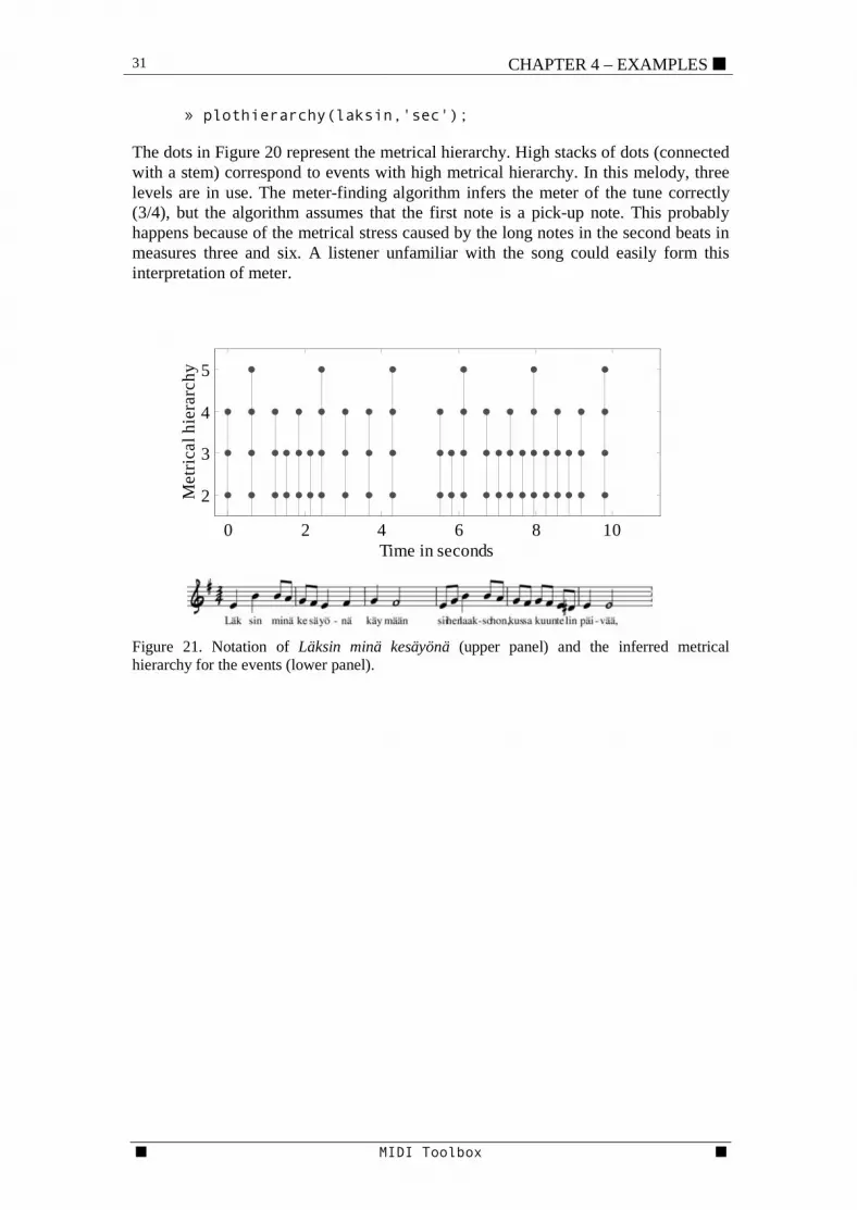
» plothierarchy(laksin,'sec'); The dots in Figure 20 represent the metrical hierarchy. High stacks of dots (connected with a stem) correspond to events with high metrical hierarchy. In this melody, three levels are in use. The meter-finding algorithm infers the meter of the tune correctly (3/4), but the algorithm assumes that the first note is a pick-up note. This probably happens because of the metrical stress caused by the long notes in the second beats in measures three and six. A listener unfamiliar with the song could easily form this interpretation of meter.
Figure 21. Notation of Läksin minä kesäyönä (upper panel) and the inferred metrical hierarchy for the events (lower panel).
0 2 4 6 8 10
2
3
4
5
Time in seconds
Met
rical
hie
rarc
hy

■ CHAPTER 4 – EXAMPLES 32
■ MIDI Toolbox ■
Example 5: Melodic Segmentation
One of the fundamental processes in perceiving music is the segmentation of the auditory stream into smaller units, melodic phrases, motifs and such issues. Various computational approaches to segmentation have been taken. With symbolic representations of music, we can distinguish rule-based and statistical (or memory-based) approaches. An example of the first category is the algorithm by Tenney and Polansky (1980), which finds the locations where the changes in “clangs” occur. These clangs correspond to large pitch intervals and large inter-onset-intervals (IOIs). This idea is partly based on Gestalt psychology. For example, this algorithm segments Läksin in the following way: » segmentgestalt(laksin,'fig');
Figure 22. Segmented version of Läksin minä kesäyönä. The dotted line indicates clang boundaries and the black line indicates the segment boundary, both the result of the Gestalt-based algorithm (Tenney & Polansky, 1980).
Another segmentation technique uses the probabilities derived from the analysis of melodies (e.g., Bod, 2002). In this technique, demonstrated in Figure 22, the probabilities of phrase boundaries have been derived from pitch-class-, interval- and duration distributions at the segment boundaries in the Essen folk song collection. » segmentprob(laksin,.6,'fig');
0 2 4 6 8 10 12 14 16C4#
D4
D4#
E4
F4
F4#
G4
G4#
A4
A4#
B4
C5
C5#
Time in beats
Pitc
h

33 CHAPTER 4 – EXAMPLES ■
■ MIDI Toolbox ■
Figure 23. Segmentation based on the probabilities of tone, interval, and duration distributions at segment boundaries in the Essen collection. The middle panel shows the probabilities of segment boundaries by the algorithm. The tune contains the two first phrases of Läksin minä kesäyönä.
Both segmentation algorithms produce plausible divisions of the example tune although the correct segmentation is more in line with Tenney & Polansky’s model. Finally, a Local Boundary Detection Model by Cambouropoulos (1997) is a recent variant of the rule-based model that offers effective segmentation of monophonic input. » boundary(laksin,'fig');
Figure 24. Segmentation of Läksin minä kesäyönä based on Local Boundary Detection Model (Camporopoulos, 1997)
0 2 4 6 8 10 12 14 16C4#D4 D4#E4 F4 F4#G4 G4#A4 A4#B4 C5 C5#
Time in beats
Pitc
h
0 2 4 6 8 10 12 14 160
0.5
1
0 2 4 6 8 10 12 14 16C4#D4 D4#E4 F4 F4#G4 G4#A4 A4#B4 C5 C5#
Time in beats
Pitc
h
0 2 4 6 8 10 12 14 160
0.2
0.4
0.6
0.8
1
Boun
dary
stre
ngth
s

■ CHAPTER 4 – EXAMPLES 34
■ MIDI Toolbox ■
Example 6: Melodic Expectations
Recent work on melodic expectancy has shown how music draws on common psychological principles of expectation that have been captured in Narmour’s (1990) cognitively oriented music-theoretic model. The model draws on the Gestalt-based principles of proximity, similarity, and good continuation and has been found to predict listeners’ melodic expectancies fairly well (Krumhansl, 1995a, b). The model operates by looking at implicative intervals and realized intervals. The former creates implications for the melody's continuation and the next interval carries out its implications (Figure 25).
Figure 25. An example implicative and realized interval.
The model contains five principles (Registral Direction, Intervallic Difference, Registral Return, Proximity, and Closure) that are each characterized by a specific rule describing the registral direction and the distance in pitch between successive tones. The principle of Registral Return, for example, refers to cases in which the second tone of the realized interval is within two semitones of the first tone of the implicative interval. According to the theory, listeners expect skips to return to proximate pitch. The combinations of implicative intervals and realized intervals that satisfy this principle are shown by the shaded area at the Figure 26.
Figure 26. Demonstration of Registral Return in Narmour’s implication-realization model. The vertical axis corresponds to the implicative interval ranging from 0 to 11 semitones. The horizontal axis corresponds to the realized interval, ranging from 12 semitones in the opposite direction of the implicative interval to 12 semitones in the same direction of the implicative interval. The shaded grids indicate the combinations of implied and realized intervals that fulfil the principle. A small X is displayed where the example fragment from Figure 25 would be positioned along the grid. According to the principle of Registral Return, the example
-12 -10 -8 -6 -4 -2 0 2 4 6 8 10 12
0
1
2
3
4
5
6
7
8
9
10
11
Imp
licat
ive
inte
rval
Realized interval
X

35 CHAPTER 4 – EXAMPLES ■
■ MIDI Toolbox ■
fragment (containing intervals of 2 semitones + 2 semitones) would not be predictable according to the algorithm as it lies outside the shaded area.
The implication-realization model has been quantified by Krumhansl (1995b), who also added a new principle, Consonance, to the model. The Figure 27 displays the quantification schemes of all six principles in Narmour’s model, available in the Toolbox as narmour function.
Figure 27. Quantification of Narmour's Implication-realization model (Krumhansl, 1995b). The darker areas indicate better realization of implied intervals. A cursory look at the shaded areas of Figure 27 indicates that proximate pitches (Proximity), reversals of direction in large intervals (Registral Direction) and unisons, perfect fourths, fifths and octaves (Consonance) are preferred as realized intervals by Narmour’s model. Other factors affect melodic expectations as well. The local key context is also a strong influence on what listeners expect of melodic continuations. If the key of the passage is known, tonal stability values (obtained from the experiment by Krumhansl & Kessler, 1982, shown in Figure 12) can be used to evaluate the degree of fitness of individual tones to the local key context. tonality function in the MIDI toolbox can be used to assign these values to note events assuming the key is in C major or C minor. In addition, differences in tonal strengths of the individual pitch-classes form asymmetrical relationships between the adjacent pitches. Tonally unstable tones tend to be attracted to tonally stable tones (e.g., in C major, B is pulled towards the tonic C, and G to either A or G). This melodic attraction (Lerdahl, 1996) provides an account
−12−10 −8 −6 −4 −2 0 2 4 6 8 10 120123456789
1011
Imp
lica
tive
inte
rval
Closure
−12−10 −8 −6 −4 −2 0 2 4 6 8 10 120123456789
1011
Imp
lica
tive
inte
rval
Registral Direction
−12−10 −8 −6 −4 −2 0 2 4 6 8 10 120123456789
1011
Imp
lica
tive
inte
rval
Registral Return
−12−10 −8 −6 −4 −2 0 2 4 6 8 10 120123456789
1011
Imp
lica
tive
inte
rval
Proximity
−12−10 −8 −6 −4 −2 0 2 4 6 8 10 120123456789
1011
Imp
lica
tive
inte
rval
Realized interval
Consonance
−12−10 −8 −6 −4 −2 0 2 4 6 8 10 120123456789
1011
Imp
lica
tive
inte
rval
Realized interval
Intervallic Difference

■ CHAPTER 4 – EXAMPLES 36
■ MIDI Toolbox ■
Mean
Tonality Proximity. Reg. Ret. Cons. Tessitura Mobility0
0.5
1
1
Model predictions
Tonality Proximity. Reg. Ret. Cons. Tessitura Mobility0
0.5
1
2
Tonality Proximity. Reg. Ret. Cons. Tessitura Mobility0
0.5
1
3
Tonality Proximity. Reg. Ret. Cons. Tessitura Mobility0
0.5
1
4
for the attraction across the pitches in tonal pitch space. This model can be evoked by the melattraction function. Finally, recent revisions of Narmour’s model by von Hippel (2000) offer a solution to melodic expectancy that is connected to the restrictions of melodic range, which have probably originated from the limitations of vocal range. These reformulations are called tessitura and mobility (and these are available in the Toolbox as functions tessitura and mobility). The former predicts that forth-coming tones will be close to median pitch height. The latter uses autocorrelation between successive pitch heights to evaluate whether the tone is predictable in relation to the previous intervals and the mean pitch. Next, we can explore how suitable three alternate continuations are to our example tune Läksin using the above-mentioned principles of melodic expectancy.
Figure 28. Fitness of four melodic continuations to a segment of the Läksin tune according to six different predictions.
In Figure 28 the Läksin tune is interrupted at the middle of a phrase and three alternative continuations in addition to the actual continuation (G) are proposed. The model predictions for each of these tones are shown below the notation. The actual tone receives the highest mean score and the chromatic tones (E and G) receive the lowest mean scores. The individual predictions of the different models illuminate why these candidates receive different fitness rating according to the models. The tone G, the highest candidate, is appropriate to continue the sequence because of its close proximity to the previous and median tone of the sequence, high degree of tonal stability of the mediant tone (G) in e-minor and because its movement direction can be predicted from the previous pitch heights. The lowest candidate G is also close in pitch proximity but it is not tonally stable and it also forms dissonant interval with the previous tone. Note that not all principles are commonly needed to estimate the fitness of a given tone to a sequence and the exact weights of the principles vary across music styles. Furthermore, this method does not explicitly account for longer pitch patterns although it is evident that in the example melody, listeners have already come across similar melodic phrase in the beginning of the melody. However, these issues can be examined using contour-related (Example 2) and continuous models (Example 7).
Continuations Context

37 CHAPTER 4 – EXAMPLES ■
■ MIDI Toolbox ■
Example 7: Melodic Complexity
Occasionally, it is interesting to know how complicated, difficult or ‘original’ a melody is. For example, Dean Keith Simonton (1984, 1994) analyzed a large number of classical themes and noticed that the originality of the themes is connected with their popularity. This relationship is in the form of inverted-U function where the most popular themes are of medium originality. As a result, the most simple themes are not popular (they may be considered ‘banal’) and neither are the most complex ones. There are also other uses for a melodic complexity measure such as using it as an aid in classification of melodic material (Toiviainen & Eerola, 2001). Simonton’s model of melodic originality is based on tone-transition probabilities. The output of this model (compltrans) produces an inverse of the averaged probability, scaled between 0 and 10 where higher value indicates higher melodic originality. Another way of assessing melodic complexity is to focus on tonal and accent coherence, and to the amount of pitch skips and contour self-similarity the melody exhibits. This model has been coined expectancy-based model (Eerola & North, 2000) of melodic complexity because the components of the model are derived from melodic expectancy theories (available as complebm function). An alternative measure of melodic complexity is anchored in continuous measurement of note event distribution (pitch-class, interval) entropy (use movewindow and entropy and various distribution functions). This measure creates melodic predictability values for each point in the melody (hence the term continuous). These values have been found to correspond to the predictability ratings given by listeners in experiments (Eerola et al., 2002). This measure offers a possibility to observe the moment-by-moment fluctuations in melodic predictability.
0 5 10 15 20 25
0
0.2
0.4
0.6
0.8
1
Pre
dict
abili
ty
Bar numbers
P-C entropy
Figure 29. Predictability of Bach’s Sarabande (first 27 measures).
The Figure 29 displays how the predictability fluctuates over time. In the beginning, predictability increases as the opening melodic motifs are repeated (see Figure 4 for notation). At measure 20, the Sarabande takes a new turn, modulates and contains large pitch skips all that lead to lower predictability values.
■ CHAPTER 4 – EXAMPLES 38
■ MIDI Toolbox ■
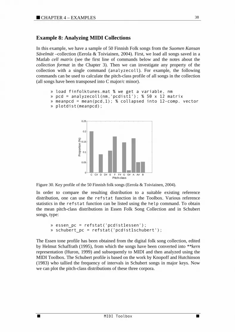
Example 8: Analyzing MIDI Collections
In this example, we have a sample of 50 Finnish Folk songs from the Suomen Kansan Sävelmät –collection (Eerola & Toiviainen, 2004). First, we load all songs saved in a Matlab cell matrix (see the first line of commands below and the notes about the collection format in the Chapter 3). Then we can investigate any property of the collection with a single command (analyzecoll). For example, the following commands can be used to calculate the pitch-class profile of all songs in the collection (all songs have been transposed into C major/c minor). » load finfolktunes.mat % we get a variable, nm » pcd = analyzecoll(nm,'pcdist1'); % 50 x 12 matrix » meanpcd = mean(pcd,1); % collapsed into 12-comp. vector » plotdist(meanpcd);
C C# D D# E F F# G G# A A# B0
0.05
0.1
0.15
0.2
0.25
Pitch-class
Pro
porti
on (%
)
Figure 30. Key profile of the 50 Finnish folk songs (Eerola & Toiviainen, 2004).
In order to compare the resulting distribution to a suitable existing reference distribution, one can use the refstat function in the Toolbox. Various reference statistics in the refstat function can be listed using the help command. To obtain the mean pitch-class distributions in Essen Folk Song Collection and in Schubert songs, type: » essen_pc = refstat('pcdist1essen'); » schubert_pc = refstat('pcdist1schubert'); The Essen tone profile has been obtained from the digital folk song collection, edited by Helmut Schaffrath (1995), from which the songs have been converted into **kern representation (Huron, 1999) and subsequently to MIDI and then analyzed using the MIDI Toolbox. The Schubert profile is based on the work by Knopoff and Hutchinson (1983) who tallied the frequency of intervals in Schubert songs in major keys. Now we can plot the pitch-class distributions of these three corpora.
39 CHAPTER 4 – EXAMPLES ■
■ MIDI Toolbox ■
C C# D D# E F F# G G# A A# B0
0.05
0.1
0.15
0.2
0.25
0.3
Pro
porti
on
Pitch-class
Finnish CollectionEssen Collection Classical (major)
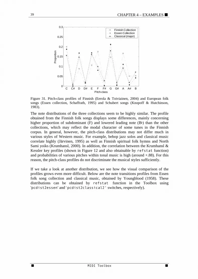
Figure 31. Pitch-class profiles of Finnish (Eerola & Toiviainen, 2004) and European folk songs (Essen collection, Schaffrath, 1995) and Schubert songs (Knopoff & Hutchinson, 1983).
The note distributions of the three collections seem to be highly similar. The profile obtained from the Finnish folk songs displays some differences, mainly concerning higher proportion of subdominant (F) and lowered leading note (B) than the other collections, which may reflect the modal character of some tunes in the Finnish corpus. In general, however, the pitch-class distributions may not differ much in various styles of Western music. For example, bebop jazz solos and classical music correlate highly (Järvinen, 1995) as well as Finnish spiritual folk hymns and North Sami yoiks (Krumhansl, 2000). In addition, the correlation between the Krumhansl & Kessler key profiles (shown in Figure 12 and also obtainable by refstat function) and probabilities of various pitches within tonal music is high (around +.88). For this reason, the pitch-class profiles do not discriminate the musical styles sufficiently. If we take a look at another distribution, we see how the visual comparison of the profiles grows even more difficult. Below are the note transitions profiles from Essen folk song collection and classical music, obtained by Youngblood (1958). These distributions can be obtained by refstat function in the Toolbox using 'pcdist2essen' and'pcdist2classical2' switches, respectively).

■ CHAPTER 4 – EXAMPLES 40
■ MIDI Toolbox ■
Figure 32. Note transitions in classical music (Youngblood, 1958) and Essen collection (Schaffrath, 1995).
In Figure 32, note repetitions have been omitted from the profile describing note transitions in the Essen collection, as Youngblood (1958) did not originally tally them. Thus, the diagonals of both profiles are empty. The common transitions, C-D, D-C, F-E, G-C, G-F, E-C, C-B, seem to occur with similar frequency in the two collections, but it is difficult to say how different the profiles actually are. A distance metric can be used to calculate the degree of similarity of the profiles. Several distance metrics can be used: Pearson’s correlation coefficient is commonly employed, although it is problematic, as it does not consider absolute magnitudes and note events in music are not normally distributed in the statistical sense (Toiviainen, 1996). A more consistent (dis)similarity measure is the Euclidean distance between the two vectors representing the distributions. Chi-square measure is another method of comparison. In addition, city block distance or cosine direction measures may be used to calculate the distances between the distributions (Everitt & Rabe-Hesketh, 1997). Some of these distance measures are considered in more detail in Example 8 (Chapter 5).
C C#DD#E
F F#GG#A
A#B
CC#DD#EFF#GG#AA#B0
0.02
0.04
0.06
2nd tone
Note transitions in Classical music
1st toneC C#D
D#EF F#G
G#AA#B
CC#DD#EFF#GG#AA#B0
0.02
0.04
0.06
2nd tone
Note transitions in Essen Folk Collection
1st tone
41 CHAPTER 4 – EXAMPLES ■
■ MIDI Toolbox ■
Example 9: Melodic similarity
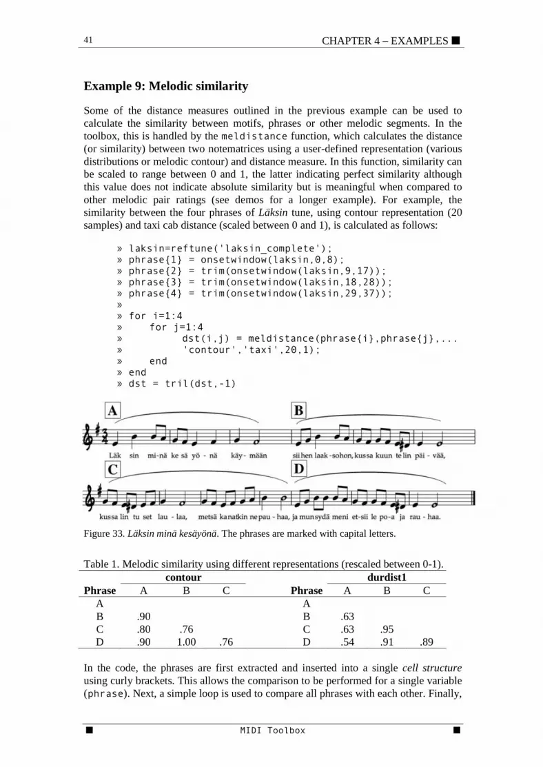
Some of the distance measures outlined in the previous example can be used to calculate the similarity between motifs, phrases or other melodic segments. In the toolbox, this is handled by the meldistance function, which calculates the distance (or similarity) between two notematrices using a user-defined representation (various distributions or melodic contour) and distance measure. In this function, similarity can be scaled to range between 0 and 1, the latter indicating perfect similarity although this value does not indicate absolute similarity but is meaningful when compared to other melodic pair ratings (see demos for a longer example). For example, the similarity between the four phrases of Läksin tune, using contour representation (20 samples) and taxi cab distance (scaled between 0 and 1), is calculated as follows: » laksin=reftune('laksin_complete'); » phrase{1} = onsetwindow(laksin,0,8); » phrase{2} = trim(onsetwindow(laksin,9,17)); » phrase{3} = trim(onsetwindow(laksin,18,28)); » phrase{4} = trim(onsetwindow(laksin,29,37)); » » for i=1:4 » for j=1:4 » dst(i,j) = meldistance(phrase{i},phrase{j},... » 'contour','taxi',20,1); » end » end » dst = tril(dst,-1)
Figure 33. Läksin minä kesäyönä. The phrases are marked with capital letters.
Table 1. Melodic similarity using different representations (rescaled between 0-1).
contour durdist1 Phrase A B C Phrase A B C
A A B .90 B .63 C .80 .76 C .63 .95 D .90 1.00 .76 D .54 .91 .89
In the code, the phrases are first extracted and inserted into a single cell structure using curly brackets. This allows the comparison to be performed for a single variable (phrase). Next, a simple loop is used to compare all phrases with each other. Finally,

■ CHAPTER 4 – EXAMPLES 42
■ MIDI Toolbox ■
the lower part of the resulting 4 x 4 matrix are displayed using tril function, shown in Table 1. The table also displays the similarities using another representation, namely distribution of durations ('durdist1' parameter in the meldistance function). Figure 33 illustrates the phrases involved in the comparison. For the contour representation, the phrases B and D are identical (similarity 1.00) and the phrase C differs most from the other phrases. This seems intuitively reasonable although the exact numbers should be viewed with caution. However, similarity based on the distribution of note durations indicates greatest similarity between the phrases B and C (.95) and lowest similarity between A and D (.54). The results of this simple indicator of rhythmic similarity are in contrast with the contour representation. These results are, again, readily apparent from the notated score. Another common comparison strategy between melodic segments involves dynamic programming, which is not covered in this tutorial (see e.g., Stammen, & Pennycook, 1993; Hu, Dannenberg & Lewis, 2002).

43 CHAPTER 4 – EXAMPLES ■
■ MIDI Toolbox ■
Example 10: Creating Sequences
The Toolbox may be used to create melodies and chord sequences that can, in turn, be saved as MIDI or synthesized audio files. For example, to recreate the chord context version of the well-known probe-tone sequences (Krumhansl & Kessler, 1982), use createnmat function. » IV = createnmat([65 69 72],0.5); » IV = setvalues(IV,'onset',0); » V = shift(IV,'pitch',2); » V = shift(V,'onset',0.75,'sec'); » I = shift(V,'pitch',-7); » I = shift(I,'onset',0.75,'sec'); » probe = createnmat([61],0.5); » probe = shift(probe,'onset', 3, 'sec'); » sequence = [IV; V; I; probe]; The first line creates a IV chord in C major (F A C) that lasts for 0.5 seconds and starts at 0 seconds (second line). The third line transposes the first chord (IV) major second up and shifts the onset time by 0.75 so that this chord (V) follows the first chord after 0.25 second pause. The fifth and sixth line repeats this operation for the third chord (I). Lines seven and eight create the probe-tone (C) and the final line combines the individual chords and the probe-tone into a sequence. To synthesize the sequence using Shepard tones, which de-emphasize pitch height and underline pitch-class, use the nmat2snd function. The following creates the probe sequence as a CD-quality audio file using the Shepard tones: » signal = nmat2snd(sequence,'shepard',44100); % » plot(signal) % create a plot of the signal » l=length(signal); » ylabel('Amplitude'); xlabel('Time (in s)') % labels » set(gca,'XTick',(0:22050:l)) » set(gca,'XTickLabel',(0:22050:l)/44100) % in seconds
Figure 34. The probe sequence as an audio signal (mono).
In most circumstances, the sampling rate (the second parameter, 44100 samples per second in the example above) can be left out. In that case, considerably lower but sufficient sampling rate (8192 Hz) is used. To play and write the signal to your hard-drive, use Matlab’s own functions soundsc and wavwrite:
0 0.5 1 1.5 2 2.5 3 3.5−1
−0.5
0
0.5
1
Am
plit
ud
e
Time (in s)
■ CHAPTER 4 – EXAMPLES 44
■ MIDI Toolbox ■
» soundsc(signal,44100); % play the synthesized sequence » wavwrite(signal,44100,'probe.wav'); % write audio file Note that in order to create a stereo audio file the signal must be in two channels, easily created by duplicating the signal to two channels: » stereo = [signal; signal]'; To demonstrate the so-called Shepard illusion (Shepard, 1964), where a scale consisting of semitones is played over four octaves using Shepard tones, type: » playsound(createnmat([48:96],.5),'shepard'); Shepard tones are ambiguous in terms of their pitch height although their pitch-class or pitch chroma can be discerned. When 12 chromatic tones are played in ascending order over and over again, an illusion of a continuous ascending pitch sequence will form although the point at which the sequence starts over is not perceived. Hearing pairs of tones in succession will form a perception of an ascending or a descending interval. When tritone intervals (e.g., C-F) are played using Shepard tones, the direction of the interval is ambiguous. Sometimes listeners hear certain tritones as ascending and sometimes descending. To listen to the tritone paradox (see Deutsch, 1991; Repp, 1994), type: » playsound(reftune('tritone'),'shepard'); Perception of interleaved melodies provides another example of melody creation. In interleaved melodies, successive notes of the two different melodies are interleaved so that the first note of the first melody is followed by the first note of second melody, followed by the second note of the first melody followed by the second note of the second melody and so on. Using these kinds of melodies in perceptual experiments, Dowling (1973; and later Hartmann & Johnson, 1991) has observed that listeners’ ability to recognize the melodies is highly sensitive to the pitch overlap of the two melodies. When the melodies are transposed so that their mean pitches are different, recognition scores increase. Create these melodies using reftune and trans functions and test at which pitch separation level you spot the titles of the songs. » d1 = reftune('dowling1',0.4); » d2 = reftune('dowling2',0.4); » d2=shift(d2,'onset',+.2,'sec'); % delay (0.2 sec) » d2=shift(d2,'dur',-.2,'sec'); % shorten the notes » d1=shift(d1,'dur',-.2,'sec'); % shorten the notes » playsound([d1; d2]); pause » playsound([d1;shift(d2,'pitch',-3)]); pause » playsound([d1;shift(d2,'pitch',6)]); pause » playsound([d1;shift(d2,'pitch',-9)]);

45 CHAPTER 4 – EXAMPLES ■
■ MIDI Toolbox ■
References
Bharucha, J. J. (1984). Anchoring effects in music: The resolution of dissonance. Cognitive Psychology, 16, 485-518.
Bod, R. (2002). Memory-based models of melodic analysis: challenging the gestalt principles. Journal of New Music Research, 31, 27-37.
Box, G. E. P., Jenkins, G., & Reinsel, G. C. (1994). Time series analysis: Forecasting and control. Englewood Cliffs, NJ: Prentice Hall.
Brown, J. C. (1993). Determination of meter of musical scores by autocorrelation. Journal of Acoustical Society of America, 94(4), 1953-1957.
Cambouropoulos, E. (1997). Musical rhythm: A formal model for determining local boundaries, accents and metre in a melodic surface. In M. Leman (Ed.), Music, Gestalt, and Computing: Studies in Cognitive and Systematic Musicology (pp. 277-293). Berlin: Springer Verlag.
Deutsch, D. (1991). The tritone paradox: An influence of language on music perception. Music Perception, 8, 335-347.
Dowling, W. J. (1973). The perception of interleaved melodies, Cognitive Psychology,5, 322-337.
Dowling, W. J. (1978). Scale and contour: Two components of a theory of memory for melodies. Psychological Review, 85(4), 341-354.
Dowling, W. J., & Fujitani, D. S. (1971). Contour, interval, and pitch recognition in memory for melodies. Journal of the Acoustical Society of America, 49, 524-531.
Dowling, W. J. & Harwood, D. L. (1986). Music cognition. Orlando: Academic Press. Eerola, T., Himberg, T., Toiviainen, P., & Louhivuori, J. (submitted). Perceived complexity
of Western and African folk melodies by Western and African listeners. Eerola, T., & North, A. C. (2000). Expectancy-based model of melodic complexity. In
Woods, C., Luck, G.B., Brochard, R., O'Neill, S. A., and Sloboda, J. A. (Eds.) Proceedings of the Sixth International Conference on Music Perception and Cognition. Keele, Staffordshire, UK: Department of Psychology. CD-ROM.
Eerola, T., Toiviainen, P., & Krumhansl, C. L. (2002). Real-time prediction of melodies: Continuous predictability judgments and dynamic models. In C. Stevens, D. Burnham, G. McPherson, E. Schubert, J. Renwick (Eds.) Proceedings of the 7th International Conference on Music Perception and Cognition, Sydney, 2002. Adelaide: Causal Productions.
Eerola, T., & Toiviainen, P. (2004). Suomen kansan esävelmät: Digital archive of Finnish Folk songs [computer database]. Jyväskylä: University of Jyväskylä. URL: http://www.jyu.fi/musica/sks/
Essens, P. (1995). Structuring temporal sequences: Comparison of models and factors of complexity. Perception & Psychophysics, 57, 519-532.
Everitt, B. S., & Rabe-Hesketh, S. (1997). The analysis of proximity data. London: Arnold. Hartmann, W. M., & Johnson, D. (1991). Stream segregation and peripheral channeling.
Music Perception, 9(2), 155-183. Hewlett, W. B. & Selfridge-Field, E. (Eds.) (1993/1994). Computing in Musicology: An
International Directory of Applications, Vols 9. Menlo Park, California: Center for Computer Assisted Research in the Humanities.
von Hippel, P. (2000). Redefining pitch proximity: Tessitura and mobility as constraints on melodic interval size. Music Perception, 17 (3), 315-327.
Hu, N., Dannenberg, R. B., & Lewis, A. L. (2002). A probabilistic model of melodic similarity. Proceedings of the 2002 International Computer Music Conference. San Francisco: International Computer Music Association, pp. 509-15.
Huron, D. (1996). The melodic arch in Western folksongs. Computing in Musicology, 10, 3-23.
Huron, D. (1999). Music research using humdrum: A user’s guide. Stanford, CA: Center for Computer Assisted Research in the Humanities.
■ CHAPTER 4 – EXAMPLES 46
■ MIDI Toolbox ■
Huron, D., & Royal, M. (1996). What is melodic accent? Converging evidence from musical practice. Music Perception, 13, 489-516.
Järvinen, T. (1995). Tonal hierarchies in jazz improvisation. Music Perception, 12(4), 415-437.
Kim, Y. E., Chai, W., Garcia, R., & Vercoe, B. (2000). Analysis of a contour-based representation for melody. In International Symposium on Music Information Retrieval, Plymouth, MA: Indiana University.
Knopoff, L. & Hutchinson, W. (1983). Entropy as a measure of style: The influence of sample length. Journal of Music Theory, 27, 75-97.
Krumhansl, C. L., & Kessler, E. J. (1982). Tracing the dynamic changes in perceived tonal organization in a spatial representation of musical keys. Psychological Review, 89, 334-368.
Krumhansl, C. L. (1990). Cognitive foundations of musical pitch. New York: Oxford University Press.
Krumhansl, C. L. (1995a). Effects of musical context on similarity and expectancy. Systematische musikwissenschaft, 3, 211-250.
Krumhansl, C. L. (1995b). Music psychology and music theory: Problems and prospects. Music Theory Spectrum, 17, 53-90.
Leman, M., Lesaffre, M., & Tanghe, K. (2000). The IPEM toolbox manual. University of Ghent, IPEM-Dept. of Musicology: IPEM.
Lemström, K., Wiggins, G. A., & Meredith, D. (2001). A three-layer approach for music retrieval in large databases. In The Second Annual Symposium on Music Information Retrieval (pp. 13-14), Bloomington: Indiana University.
Lerdahl, F. (1996). Calculating tonal tension. Music Perception, 13(3), 319-363. Lerdahl, F., & Jackendoff, R. (1983). A generative theory of tonal music. Cambridge: MIT
Press. Palmer, C., & Krumhansl, C. L. (1987). Independent temporal and pitch structures in
determination of musical phrases. Journal of Experimental Psychology: Human Perception and Performance, 13, 116-126.
Repp, B. (1994). The tritone paradox and the pitch range of the speaking voice: A dubious connection. Music Perception, 12, 227-255.
Schellenberg, E. G. (1996). Expectancy in melody: Tests of the implication-realization model. Cognition, 58, 75-125.
Schellenberg, E. G. (1997). Simplifying the implication-realization model of melodic expectancy. Music Perception, 14, 295-318.
Shepard, R. N. (1964). Circularity in judgements of relative pitch. Journal of the Acoustical Society of America, 36, 2346-2353.
Simonton, D. K. (1984). Melodic structure and note transition probabilities: A content analysis of 15,618 classical themes. Psychology of Music, 12, 3-16.
Simonton, D. K. (1994). Computer content analysis of melodic structure: Classical composers and their compositions. Psychology of Music, 22, 31-43.
Schaffrath, H. (1995). The Essen Folksong Collection in Kern Format. [computer database] D. Huron (Ed.). Menlo Park, CA: Center for Computer Assisted Research in the Humanities.
Stammen, D., & Pennycook, B. (1993). Real-time recognition of melodic fragments using the dynamic timewarp algorithm. Proceedings of the 1993 International Computer Music Conference. San Francisco: International Computer Music Association, pp. 232-235.
Tenney, J., & Polansky, L. (1980). Temporal gestalt perception in music. Journal of Music Theory, 24(2), 205-41.
Thompson, W. F. (1994). Sensitivity to combinations of musical parameters: Pitch with duration, and pitch pattern with durational pattern. Perception & Psychophysics, 56, 363-374.
Toiviainen, P. (1996). Modelling musical cognition with artificial neural networks. Unpublished PhD dissertation, Jyväskylä Studies in the Arts 51. Jyväskylä, Finland: University of Jyväskylä.

47 CHAPTER 4 – EXAMPLES ■
■ MIDI Toolbox ■
Toiviainen, P., & Krumhansl, C. L. (2003). Measuring and modeling real-time responses to music: the dynamics of tonality induction. Perception, 32(6), 741-766.
Toiviainen, P., & Eerola, T. (2001). A method for comparative analysis of folk music based on musical feature extraction and neural networks. Proceedings of the VII International Symposium on Systematic and Comparative Musicology and III International Conference on Cognitive Musicology, 2001, University of Jyväskylä, Finland.
Toiviainen, P., & Eerola, T. (2004). The role of accent periodicities in meter induction: A classification study. In x (Ed.), Proceedings of the ICMPC8 (p. xxx-xxx). xxx:xxx.
Vos, P. G., & Troost, J. M. (1989). Ascending and descending melodic intervals: statistical findings and their perceptual relevance. Music Perception, 6(4), 383-396.
Youngblood, J.E. (1958). Style as information. Journal of Music Theory, 2, 24-35.

■ CHAPTER 5 – FUNCTION REFERENCE 48
■ MIDI Toolbox ■
CHAPTER 5 – FUNCTION REFERENCE This chapter contains detailed descriptions of all MIDI Toolbox functions. It begins with a list of functions grouped by subject area and continues with the reference entries in alphabetical order. Most of the subject areas are self-explanatory (plotting functions, segmentation functions) but some may need further explanation. CONVERSION FUNCTIONS convert from MIDI files to Matlab or vice versa or perform some other type of conversion. META FUNCTIONS is a special category, in which a function uses another function to perform an operation to a collection. FILTER FUNCTIONS mostly return a new NMAT that has been modified according to the particular filter used. STATISTICAL FUNCTIONS refer to various event distributions of the notematrix (proportion of pitch-classes in a notematrix, for example). The output format of the functions is indicated on the rightmost column. The following abbreviations are used:
Abbr. Explanation s Scalar r Row vector c Column vector (scalar value for each note) nm Notematrix cm Cell matrix m Matrix o Other (e.g., output can be a Figure, sound or a text string) - None

49 CHAPTER 5 – FUNCTION REFERENCE ■
■ MIDI Toolbox ■
CONVERSION FUNCTIONS Function Purpose Output dir2coll Converts a directory of MIDI files to cellmatrix structure cm hz2midi Convert frequencies to MIDI numbers c keyname Convert keys (24) to key names (text) o midi2hz Convert MIDI note numbers to frequencies (Herz) c notename Convert MIDI numbers to American pitch spelling (text) o readmidi Reads a MIDI file to a notematrix nm writemidi Writes a MIDI file from a notematrix (file)
GENERATION FUNCTIONS Function Purpose Output createnmat Create a notematrix from the input arguments nm setmidiplayer Define external MIDI player - nmat2snd Synthesize NMAT using simple synthesis o playmidi Plays NMAT using external MIDI player o playsound Play and synthesize NMAT using simple synthesis o reftune Obtain a 'reference' or example tune nm
FILTER FUNCTIONS Function Purpose Output dropmidich Note events that are not on channel CH nm dropshortnotes Returns note events that are shorter than THRESHOLD nm elim Eliminate short MIDI tracks nm extreme Returns extreme pitches (high/low) of a polyphonic NMAT nm getmidich Note events on channel CH nm ismonophonic Returns 1 if the sequence is monophonic s mchannels Midi channels that are used in NMAT r movewindow Runs a selected function within a defined time window c onsetwindow Events with mintime <= onsettime <= maxtime nm perchannel Create output for each available channel o quantize Quantize note onsets and durations of NMAT nm scale Scales note data in given dimension (time, onsets, or duration) nm setvalues Sets the chosen notematrix value for every event nm shift Shifts note data in given dimension (onset, duration, or pitch) nm transpose2c Transposes NMAT to C major/C minor nm trim Removal of leading silence (trim) nm
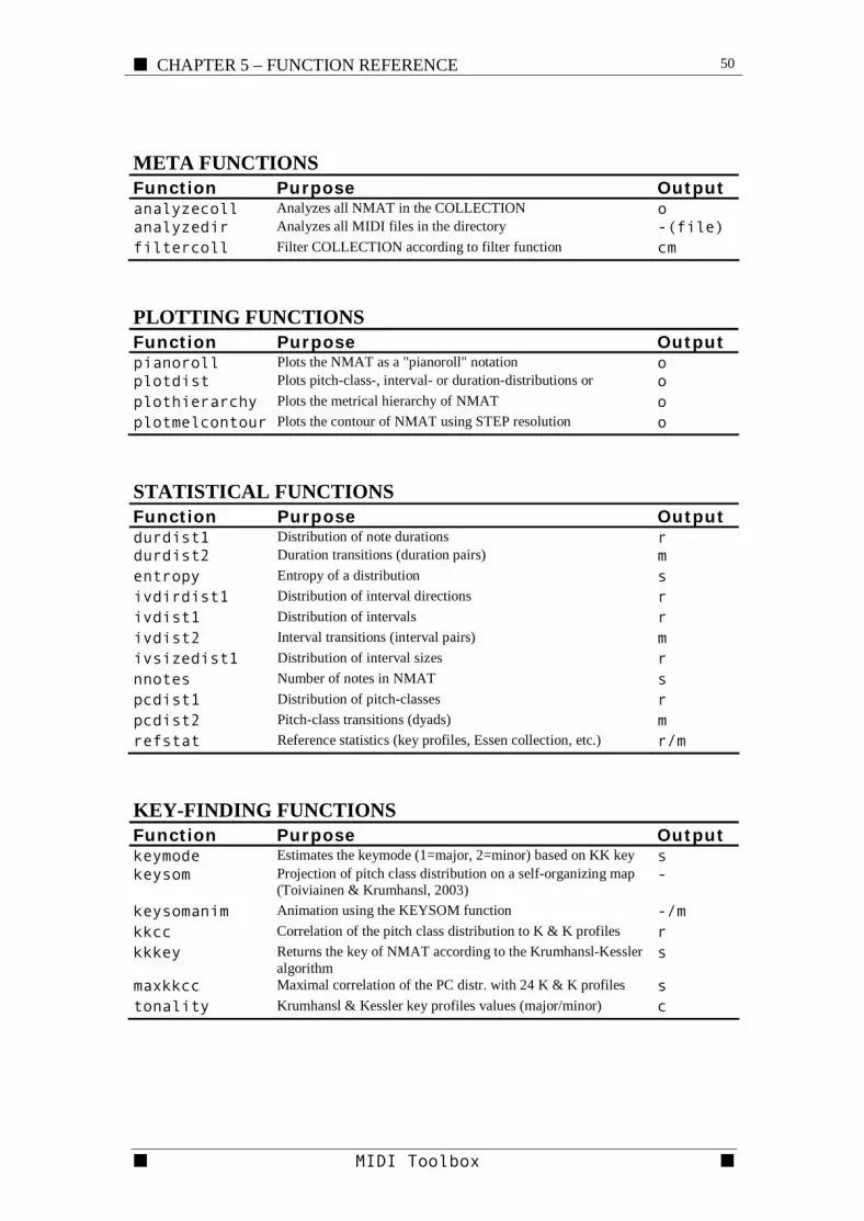
■ CHAPTER 5 – FUNCTION REFERENCE 50
■ MIDI Toolbox ■
META FUNCTIONS Function Purpose Output analyzecoll Analyzes all NMAT in the COLLECTION o analyzedir Analyzes all MIDI files in the directory -(file) filtercoll Filter COLLECTION according to filter function cm
PLOTTING FUNCTIONS Function Purpose Output pianoroll Plots the NMAT as a "pianoroll" notation o plotdist Plots pitch-class-, interval- or duration-distributions or
i io
plothierarchy Plots the metrical hierarchy of NMAT o plotmelcontour Plots the contour of NMAT using STEP resolution o
STATISTICAL FUNCTIONS Function Purpose Output durdist1 Distribution of note durations r durdist2 Duration transitions (duration pairs) m entropy Entropy of a distribution s ivdirdist1 Distribution of interval directions r ivdist1 Distribution of intervals r ivdist2 Interval transitions (interval pairs) m ivsizedist1 Distribution of interval sizes r nnotes Number of notes in NMAT s pcdist1 Distribution of pitch-classes r pcdist2 Pitch-class transitions (dyads) m refstat Reference statistics (key profiles, Essen collection, etc.) r/m
KEY-FINDING FUNCTIONS Function Purpose Output keymode Estimates the keymode (1=major, 2=minor) based on KK key s keysom Projection of pitch class distribution on a self-organizing map
(Toiviainen & Krumhansl, 2003) -
keysomanim Animation using the KEYSOM function -/m kkcc Correlation of the pitch class distribution to K & K profiles r kkkey Returns the key of NMAT according to the Krumhansl-Kessler
algorithm s
maxkkcc Maximal correlation of the PC distr. with 24 K & K profiles s tonality Krumhansl & Kessler key profiles values (major/minor) c

51 CHAPTER 5 – FUNCTION REFERENCE ■
■ MIDI Toolbox ■
CONTOUR FUNCTIONS Function Purpose Output melcontour Contour vector r combcontour Builds the Quinn (1999) representation of melodic contour m
SEGMENTATION FUNCTIONS Function Purpose Output segmentgestalt Segmentation algorithm by Tenney & Polansky (1980) c segmentprob Probabilistic estimation of segment boundaries based on the
Essen collection c
boundary Local Boundary Detection Model by Cambouropoulos (1997) c
MELODIC FUNCTIONS Function Purpose Output ambitus Melodic range in semitones s complebm Expectancy-based model of melodic complexity (Eerola &
North, 2000) s
compltrans Melodic originality measure (Simonton, 1984) s gradus Degree of melodiousness (Euler, 1739) s melaccent Melodic accent (Thomassen, 1982) c melattraction Melodic attraction (Lerdahl, 1996) c meteraccent Measure of phenomenal accent synchrony (Eerola, 2003) c mobility Melodic motion as a mobility (Hippel, 2000) c narmour Implication-realization principles by Narmour (1990) c tessitura Melodic tessitura based on deviation from median pitch height
(Hippel, 2000) c
meldistance Measurement of distance between two NMATs s
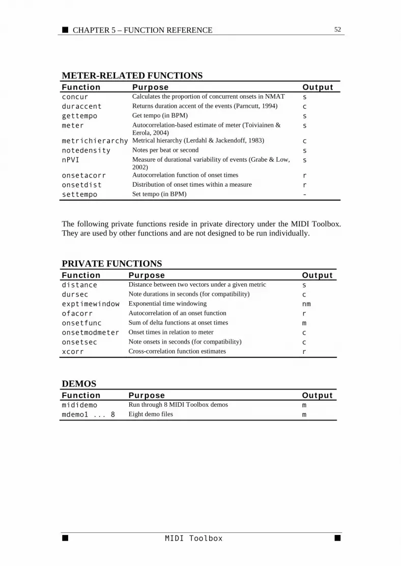
■ CHAPTER 5 – FUNCTION REFERENCE 52
■ MIDI Toolbox ■
METER-RELATED FUNCTIONS Function Purpose Output concur Calculates the proportion of concurrent onsets in NMAT s duraccent Returns duration accent of the events (Parncutt, 1994) c gettempo Get tempo (in BPM) s meter Autocorrelation-based estimate of meter (Toiviainen &
Eerola, 2004) s
metrichierarchy Metrical hierarchy (Lerdahl & Jackendoff, 1983) c notedensity Notes per beat or second s nPVI Measure of durational variability of events (Grabe & Low,
2002) s
onsetacorr Autocorrelation function of onset times r onsetdist Distribution of onset times within a measure r settempo Set tempo (in BPM) - The following private functions reside in private directory under the MIDI Toolbox. They are used by other functions and are not designed to be run individually.
PRIVATE FUNCTIONS Function Purpose Output distance Distance between two vectors under a given metric s dursec Note durations in seconds (for compatibility) c exptimewindow Exponential time windowing nm ofacorr Autocorrelation of an onset function r onsetfunc Sum of delta functions at onset times m onsetmodmeter Onset times in relation to meter c onsetsec Note onsets in seconds (for compatibility) c xcorr Cross-correlation function estimates r
DEMOS Function Purpose Output mididemo Run through 8 MIDI Toolbox demos m mdemo1 ... 8 Eight demo files m

53 CHAPTER 5 – FUNCTION REFERENCE ■
■ MIDI Toolbox ■
ambitus Function synopsis
Melodic range in semitones Function syntax
function a = ambitus(nmat) Function comments Returns the melodic rage (ambitus) in semitones of NMAT Input argument: NMAT = notematrix Output: A = melodic range in semitones Example: y = ambitus(nmat);
analyzecoll Function synopsis
Analysis of collection using a specified function Function syntax
function data = analyzecoll(coll, functionname, <other arguments>)
Function comments ANALYZECOLL works only with functions that take the notematrix as input argument and works only with functions returning either scalar or row vector. Input arguments: COLL = name of the collection FUNNAME = name of the function <OTHER ARGUMENTS> possible other arguments to be passed to function FUNNAME Output: DATA = scalar or row vector containing the output of function FUNNAME with each notematrix of the collection used as input argument Example: keys = analyzecoll(collection, 'kkkey');
See also analyzedir, filtercoll
analyzedir Function synopsis
Analysis of MIDI files in a directory
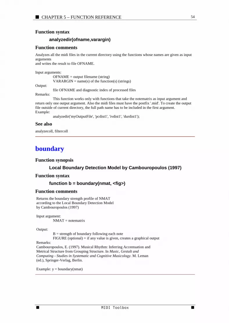
■ CHAPTER 5 – FUNCTION REFERENCE 54
■ MIDI Toolbox ■
Function syntax analyzedir(ofname,varargin)
Function comments Analyzes all the midi files in the current directory using the functions whose names are given as input arguments and writes the result to file OFNAME. Input arguments: OFNAME = output filename (string) VARARGIN = name(s) of the function(s) (strings) Output: file OFNAME and diagnostic index of processed files Remarks: This function works only with functions that take the notematrix as input argument and return only one output argument. Also the midi files must have the postfix '.mid'. To create the output file outside of current directory, the full path name has to be included in the first argument. Example: analyzedir('myOutputFile', 'pcdist1', 'ivdist1', 'durdist1');
See also analyzecoll, filtercoll
boundary Function synopsis
Local Boundary Detection Model by Cambouropoulos (1997) Function syntax
function b = boundary(nmat, <fig>) Function comments Returns the boundary strength profile of NMAT according to the Local Boundary Detection Model by Cambouropoulos (1997) Input argument: NMAT = notematrix Output: B = strength of boundary following each note FIGURE (optional) = if any value is given, creates a graphical output Remarks: Cambouropoulos, E. (1997). Musical Rhythm: Inferring Accentuation and Metrical Structure from Grouping Structure. In Music, Gestalt and Computing - Studies in Systematic and Cognitive Musicology. M. Leman (ed.), Springer-Verlag, Berlin. Example: y = boundary(nmat)
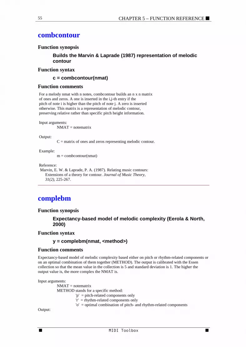
55 CHAPTER 5 – FUNCTION REFERENCE ■
■ MIDI Toolbox ■
combcontour Function synopsis
Builds the Marvin & Laprade (1987) representation of melodic contour
Function syntax c = combcontour(nmat)
Function comments For a melody nmat with n notes, combcontour builds an n x n matrix of ones and zeros. A one is inserted in the i,j-th entry if the pitch of note i is higher than the pitch of note j. A zero is inserted otherwise. This matrix is a representation of melodic contour, preserving relative rather than specific pitch height information. Input arguments: NMAT = notematrix Output: C = matrix of ones and zeros representing melodic contour. Example: m = combcontour(nmat) Reference: Marvin, E. W. & Laprade, P. A. (1987). Relating music contours: Extensions of a theory for contour. Journal of Music Theory, 31(2), 225-267.
complebm Function synopsis
Expectancy-based model of melodic complexity (Eerola & North, 2000)
Function syntax y = complebm(nmat, <method>)
Function comments Expectancy-based model of melodic complexity based either on pitch or rhythm-related components or on an optimal combination of them together (METHOD). The output is calibrated with the Essen collection so that the mean value in the collection is 5 and standard deviation is 1. The higher the output value is, the more complex the NMAT is. Input arguments: NMAT = notematrix METHOD stands for a specific method: 'p' = pitch-related components only 'r' = rhythm-related components only 'o' = optimal combination of pitch- and rhythm-related components Output:

■ CHAPTER 5 – FUNCTION REFERENCE 56
■ MIDI Toolbox ■
y = integer for complexity that is calibrated in relation to Essen Collection (Schaffrath, 1995). Higher values = higher complexity. Example: Analyze a folk tune 'laksin' for its pitch-related complexity: compl_ebm(laksin,'p') ans = 5.151 The answer means that the tune is somewhat more complicated than the average tune in Essen collection (0.151 standard deviations higher). References: Eerola, T. & North, A. C. (2000) Expectancy-Based Model of Melodic Complexity. In Woods, C.,
Luck, G.B., Brochard, R., O'Neill, S. A., and Sloboda, J. A. (Eds.) Proceedings of the Sixth International Conference on Music Perception and Cognition. Keele, Staffordshire, UK: Department of Psychology. CD-ROM.
Schaffrath, H. (1995). The Essen folksong collection in kern format. [computer database]. Menlo Park, CA: Center for Computer Assisted Research in the Humanities.
See also compltrans
compltrans Function synopsis
Melodic originality measure (Simonton, 1984) Function syntax
s = compltrans(nmat) Function comments Calculates Simonton's (1984, 1994) melodic originality score based on 2nd order pitch-class distribution of classical music that has been derived from 15618 classical music themes. Input argument: NMAT = notematrix Output: S = integer (inverse of averaged probability), scaled between 0 and 10 (higher value indicates higher melodic originality. References: Simonton, D. K. (1984). Melodic structure and note transition probabilities: A content analysis of 15,618 classical themes. Psychology of Music, 12, 3-16. Simonton, D. K. (1994). Computer content analysis of melodic structure: Classical composers and their compositions. Psychology of Music, 22, 31-43. See also complebm
concur Function synopsis
Detection of simultaneous onsets in a notematrix
57 CHAPTER 5 – FUNCTION REFERENCE ■
■ MIDI Toolbox ■
Function syntax c = concur(nmat,<threshold>)
Function comments Calculates the number of simultaneous onsets in NMAT with certain beat THRESHOLD. This function can be used in finding and eliminating short tracks in multichannel MIDI files. Input arguments: NMAT= notematrix THRESHOLD = (optional) value for threshold for concurrent onsets. Default value is ± 0.2 beats Output: C = integer displaying the proportion of concurrent onsets Remarks: Only the NOTES vector is required for the input, other input arguments are optional and will be replaced by default values if omitted. Example: concur(nmat,0.25);
See also channel, elim
createnmat Function synopsis
Create isochronous notematrix Function syntax
nmat = createnmat(notes,<dur>,<vel>,<ch>) Function comments Function creates a notematrix of isochronous pitches based on the NOTES vector. This is useful for demonstration purposes and for creating stimuli with certain properties. Input arguments: NOTES = pitch vector (e.g., [60 64 67] for C major chord) DUR (optional) = note durations in seconds (default 0.25) VEL (optional) = note velocities (0-127, default 100) CH (optional) = note channel (default 1) Output: NMAT = notematrix Remarks: Only the NOTES vector is required for the input, other input arguments are optional and will be replaced by default values if omitted. Example: Create major scale going up major = [0 2 4 5 7 9 11 12] + 60; nmat = createnmat(major,0.2);

■ CHAPTER 5 – FUNCTION REFERENCE 58
■ MIDI Toolbox ■
dir2coll Function synopsis
Conversion of directory of midi files to cell matrix Function syntax
[nm,name] = dir2coll(ofname) Function comments Function converts all MIDI files in a directory to cellmatrix structure (NM). The filenames are also saved (NAME). If output filename (ofname) is given, the variables are saved as a Matlab *.MAT file. Input arguments: OFNAME = 'filename' (string) Output: NM = cell matrix of all MIDI files in a directory NAME = filenames (string) Remarks: If the input argument is left out, no variables are saved. Example: [nm,name] = dir2coll; Reads the midi files in the current directory to the cell matrix structure
dropmidich Function synopsis
MIDI channel based filtering of notes Function syntax
nmatf = dropmidich(nmat, ch) Function comments Filters out note events of NMAT that are on channel CH Input arguments: NMAT = notematrix CH = number of midi channel to be filtered out Output: NMATF = filtered notematrix Example: Remove drum track of general MIDI file nmatf = dropmidich(nmat,10); %
dropshortnotes Function synopsis
Filtering of short notes Function syntax
nmatf = dropshortnotes(nmat, unit, threshold)

59 CHAPTER 5 – FUNCTION REFERENCE ■
■ MIDI Toolbox ■
0 0.5 1 1.5 20
0.2
0.4
0.6
0.8
1
dura
tiona
l acc
ent
duration (in seconds)
Function comments Filters out note events in NMAT that are shorter than THRESHOLD. Input arguments: NMAT = notematrix UNIT = time unit for duration: possible values are 'sec' and 'beat' THRESHOLD = duration threshold for filtering Output: NMATF = filtered notematrix Example: Filter out notes shorter than 1/16: nmatf = dropshortnotes(nmat, 'beat', 1/16)
duraccent Function synopsis
Duration accent by Parncutt (1994) Function syntax
D = duraccent(dur,<tau>,<accent_index>) Function comments Function returns duration accent of the events (Parncutt, 1994, p. 430-431) where tau represents saturation duration, which is proportional to the duration of the echoic store. Accent index covers the minimum discriminable duration. The difference between Parncutt's model and this implementation is on the IOI (inter-onset-intervals). Input arguments: DUR = vector of note duration in seconds TAU (optional) = saturation duration (default 0.5) ACCENT_INDEX (optional) = minimum discriminable duration (default 2) Output: D = new duration vector corresponding to the size of input vector Remarks: The original model uses IOI (inter-onset-intervals) for input whereas this version takes the note duration value in seconds. Example : duracc = duraccent(dursecs(NMAT)); References: Parncutt, R. (1994). A perceptual model of pulse salience and metrical accent in musical rhythms.
Music Perception, 11(4), 409-464.
durdist1 Function synopsis
Note duration distribution
■ CHAPTER 5 – FUNCTION REFERENCE 60
■ MIDI Toolbox ■
Function syntax dd = durdist1(nmat)
Function comments Returns the distribution of note durations in NMAT as a 9-component vector. The centers of the bins are on a logarithmic scale as follows: component bin center (in units of one beat) 1 1/4 2 sqrt(2)/4 3 1/2 4 sqrt(2)/2 5 1 6 sqrt(2) 7 2 8 2*sqrt(2) 9 4 Input argument: NMAT = notematrix Output: DD = 9-component distribution of note durations
See also plotdist, refstat , ivdist1, ivdist2, pcdist1, pcdist2
durdist2 Function synopsis
Duration dyad distribution Function syntax
dd = durdist2(nmat) Function comments Returns the distribution of pairs of note durations of successive notes as a 9 * 9 matrix. For bin centers, see DURDIST1. Input argument: NMAT = notematrix Output: DD = 9 * 9 distribution matrix of note duration pairs
See also plotdist, refstat , ivdist1, ivdist2, pcdist1, pcdist2
elim Function synopsis
Elimination of "short" midi tracks
61 CHAPTER 5 – FUNCTION REFERENCE ■
■ MIDI Toolbox ■
Function syntax [nmate,coverage] = elim(nmat,<extent_crit>)
Function comments Eliminates tracks shorter than EXTENT_CRIT from NMAT. Short tracks are those that are shorter than EXTENT_CRIT as percentage of the whole duration. Input arguments: NMAT = Notematrix EXTENT_CRIT (optional) = minimum proportion of duration that is required for the track (default value is 0.5, that is, 50% coverage) Output: NMATE = new, eliminated notematrix COVERAGE = the proportion of onsets in MIDI track Remarks: This function can be used in removing extra tracks from MIDI file. Example: Eliminate those tracks that have onsets covering less than 20% of the whole duration: nmat2 =elim(nmat,0.2);
See also concur
entropy Function synopsis
Entropy of a distribution Function syntax
function h = entropy(d) Function comments Returns the relative entropy of any distribution given as input argument. Input argument: D = distribution Output: H = relative entropy (0 =< H =< 1)
extreme Function synopsis
Returns the extreme pitches (high or low) of a polyphonic NMAT Function syntax
nm2 = extreme(nmat,<meth>) Function comments Input argument: NMAT = notematrix METH (string) = method, either HIGH (default) or LOW

■ CHAPTER 5 – FUNCTION REFERENCE 62
■ MIDI Toolbox ■
Output: NM2 = monophonic notematrix containing only highest/lowest pitches Remarks: Example: Obtain a new notematrix containing only the lowest lowest pitches: nm2 = extreme(nmat,'low');
filtercoll Function synopsis
Filter collection using a specified FILTERNAME function Function syntax
data = filtercoll(coll,filtername, <varargin>) Function comments FILTERCOLL works only with functions that take the notematrix as input argument. Input arguments: COLL = name of the collection FILTERNAME = name of the FILTER function VARARGIN = possible other arguments to be passed to filter function FUNNAME Output: DATA = vector or matrix containing the output of function FUNNAME with each notematrix of the collection used as input argument. Example: fnm = filtercoll(nm, 'trans',7); % transpose the whole collection a fifth up
getmidich Function synopsis
Note events on a given MIDI channel Function syntax
nmatf = getmidich(nmat, ch) Function comments Returns note events of NMAT that are on MIDI channel CH. Input arguments: NMAT = notematrix CH = MIDI channel Output: NMATF = notematrix containing notes of NMAT that are on MIDI channel CH
See also perchannel
63 CHAPTER 5 – FUNCTION REFERENCE ■
■ MIDI Toolbox ■
gettempo Function synopsis
Get tempo (in BPM) Function syntax
bpm = gettempo(nmat) Function comments Returns the tempo of the NMAT in beat per minute (BPM). Note that MIDI files can be encoded using any arbitrary tempo and therefore the output of this function should be interpreted with caution. Input argument: NMAT = notematrix Output: BPM = tempo (in beats per minute)
See also settempo
gradus Function synopsis
Degree of melodiousness (Euler, 1739) Function syntax
y = gradus (nmat) Function comments Calculates the degree of melodiousness (gradus suavitatis), proposed by L. Euler (1707-1783). He suggested that the "degree of melodiousness depends on calculations made by the mind: fewer calculations, the more pleasant the experience. [The model] is implemented by a numerical technique based on the decomposition of natural numbers into a product of powers of different primes." (Leman, 1995, p. 5) Input argument: NMAT = notematrix Output: Y = integer (degree of melodiousness) where low value indicates high melodiousness References: Euler, L. (1739). Tentamen novae theoriae musicae. Leman, M. (1995). Music and schema theory: Cognitive foundations of systematic musicology. Berlin:
Springer.
hz2midi Function synopsis
Hertz to MIDI note number conversion
■ CHAPTER 5 – FUNCTION REFERENCE 64
■ MIDI Toolbox ■
Function syntax m = hz2midi(hertz)
Function comments Converts frequency values given in Hertz to MIDI note numbers. Notes are numbered in semitones with middle C being 60. Midi note 69 (A3) has a frequency of 440 hertz (abbreviated Hz), i.e., 440 cycles per second. Input arguments: HERTZ = frequency in hertz Output: M = MIDI numbers
See also pitch, notename
ismonophonic Function synopsis Returns 1 if NMAT is monophonic (logical function) Function syntax
l = ismonophonic(nmat,<overlap>,<timetype>) Function comments Returns 1 if the sequence has no overlapping notes in NMAT. Function is for finding errors in monophonic melodies and checking whether analysis is suitable for the selected NMAT. For example, ivdist1 cannot be meaningfully performed for a polyphonic input. Input argument: NMAT = notematrix OVERLAP (Optional) = Criteria for allowing short overlap between events. The default value is 0.1 seconds TIMETYPE (Optional) = timetype ('BEAT' or SEC (Seconds, default). Output: L = 1 is monophonic or 0 (contains overlap between the events)
ivdist1 Function synopsis
Distribution of intervals Function syntax
ivd = ivdist1(nmat) Function comments Returns the distribution of intervals in NMAT as a 25-component vector. The components are spaced at semitone distances with the first component representing the downward octave and the last component

65 CHAPTER 5 – FUNCTION REFERENCE ■
■ MIDI Toolbox ■
the upward octave. The distribution is weighted by note durations. The note durations are based on duration in seconds that are modified according to Parncutt's durational accent model (1994). Input arguments: NMAT = notematrix Output: IVD = interval distribution of NMAT
See also plotdist, refstat , durdist1, durdist2, pcdist1, pcdist2
ivdist2 Function synopsis
Distribution of interval dyads Function syntax
ivd = ivdist2(nmat) Function comments Returns the distribution of interval dyads in NMAT. The distribution is weighted by note durations. The note durations are based on duration in seconds that are modified according to Parncutt's durational accent model (1994). Input arguments: NMAT = notematrix Output: IVD = interval distribution of NMAT
See also plotdist, refstat , durdist1, durdist2, pcdist1, pcdist2
ivdirdist1 Function synopsis
Distribution of interval directions Function syntax
ivd = ivdirdist1(nmat) Function comments Returns the proportion of upward intervals for each interval size in NMAT as a 12-component vector. The components are spaced at semitone distances with the first component representing minor second and the last component the upward octave. Input arguments: NMAT = notematrix Output: IVD = interval direction distribution of NMAT

■ CHAPTER 5 – FUNCTION REFERENCE 66
■ MIDI Toolbox ■
See also plotdist, refstat , ivdist1, ivdist2, pcdist1, pcdist2, ivsizedist1
ivsizedist1 Function synopsis
Distribution of interval sizes Function syntax
ivd = ivsizedist1(nmat) Function comments Returns the distribution of interval sizes in NMAT as a 13-component vector. The components are spaced at semitone distances with the first component representing the unison and the last component the octave Input arguments: NMAT = notematrix Output: IVD = interval size distribution of NMAT Example: plotdist(ivsizedist(laksin));
See also plotdist, refstat , ivdist1, ivdist2, pcdist1, pcdist2
keymode Function synopsis
Mode (major vs. minor) estimation Function syntax
k = keymode(nmat) Function comments Functions estimates the key mode (1=major, 2=minor) based on Krumhansl-Kessler key finding algorithm and pitch distribution of the NMAT. This function is used to assign TONALITY values to NMAT. Input argument: NMAT = notematrix Output: K = estimated mode of NMAT (1=major, 2=minor) Example: k = keymode(nmat)
See also tonality, kkcc, kkkey , maxkkcc

67 CHAPTER 5 – FUNCTION REFERENCE ■
■ MIDI Toolbox ■
-1
-0.8
-0.6
-0.4
-0.2
0
0.2
0.4
0.6
0.8
1
C
Db
D
Eb
E
F
Gb
G
Ab
A
Bb
B
c
c#
d
d#
e
f
f#
g
ab
a
bb
b
keyname Function synopsis
Conversion of key numbers to key names (text) Function syntax
name=keyname(n,<detail>) Function comments Convert key numbers to key names (text). Encoding: 1 = C, 2= C#/Db, ... 13 = c, 14 = c#/db, ... Input argument: N = key codes (obtained eg. using KKKEY function) DETAIL (optional) = 1 denotes long, otherwise short (default) Output: text string
keysom Function synopsis
Projection of pitch class distribution on a self-organizing map Function syntax
function keysom(nmat,<cbar>,<cmap>,<tsize>) Function comments Creates a pseudocolor map of the pitch class distribution of NMAT projected onto a self-organizing map trained with the Krumhansl-Kessler profiles. Colors correspond to Pearson correlation values. Input argument: NMAT = notematrix CBAR (optional) = colorbar switch (1 = legend (default), 0 = no legend) CMAP (optional) = colormap (string, 'jet' (default), 'gray', etc.) TSIZE (optional) = textsize points (default = 16) References: Toiviainen, P. & Krumhansl, C. L. (2003). Measuring and modeling real-time responses to music: the dynamics of tonality induction. Perception, 32(6), 741-766. Krumhansl, C. L., & Toiviainen, P. (2001) Tonal cognition. In R. J. Zatorre & I. Peretz (Eds.), The Biological Foundations of Music.
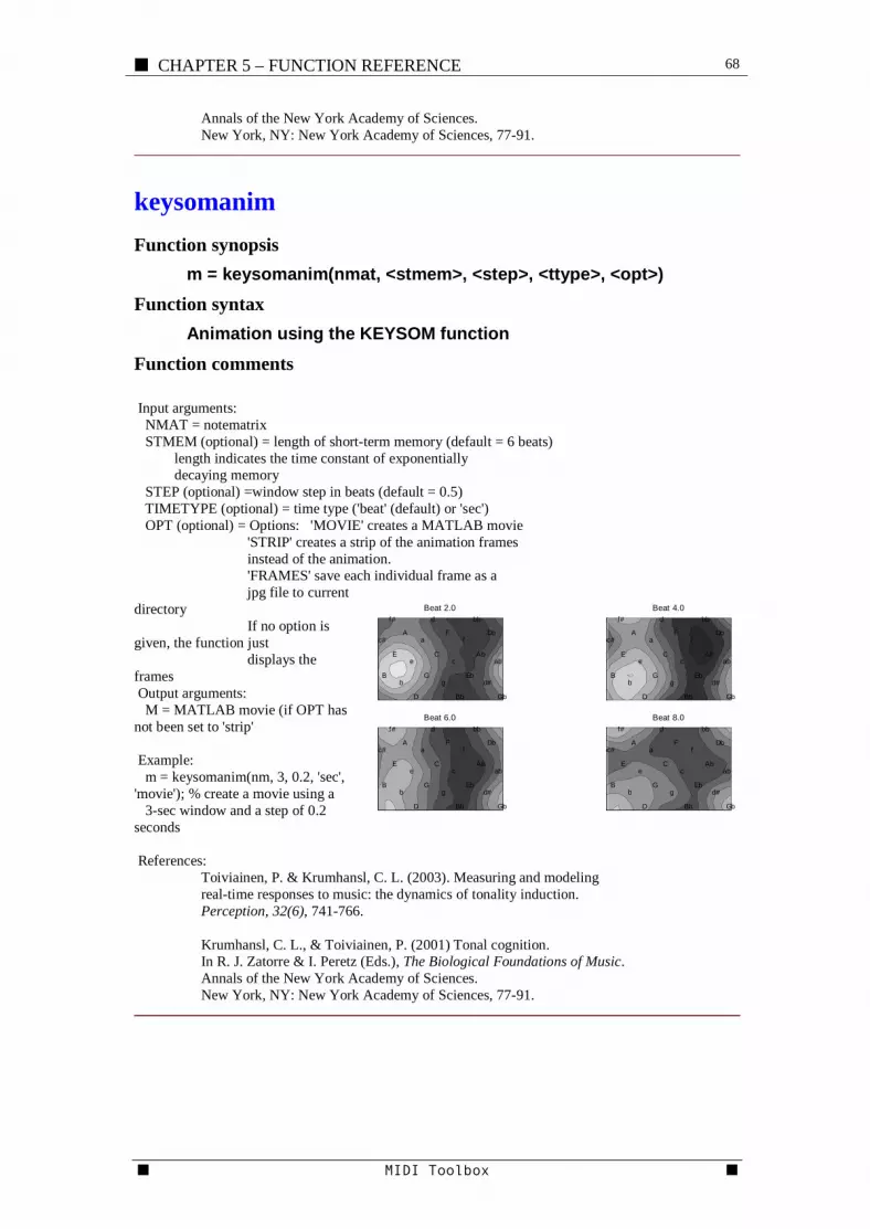
■ CHAPTER 5 – FUNCTION REFERENCE 68
■ MIDI Toolbox ■
Beat 2.0
C
Db
D
Eb
E
F
Gb
G
Ab
A
Bb
B
c
c#
d
d#
e
f
f#
g
ab
a
bb
b
Beat 4.0
C
Db
D
Eb
E
F
Gb
G
Ab
A
Bb
B
c
c#
d
d#
e
f
f#
g
ab
a
bb
b
Beat 6.0
C
Db
D
Eb
E
F
Gb
G
Ab
A
Bb
B
c
c#
d
d#
e
f
f#
g
ab
a
bb
b
Beat 8.0
C
Db
D
Eb
E
F
Gb
G
Ab
A
Bb
B
c
c#
d
d#
e
f
f#
g
ab
a
bb
b
Annals of the New York Academy of Sciences. New York, NY: New York Academy of Sciences, 77-91.
keysomanim Function synopsis
m = keysomanim(nmat, <stmem>, <step>, <ttype>, <opt>) Function syntax
Animation using the KEYSOM function Function comments Input arguments: NMAT = notematrix STMEM (optional) = length of short-term memory (default = 6 beats) length indicates the time constant of exponentially decaying memory STEP (optional) =window step in beats (default = 0.5) TIMETYPE (optional) = time type ('beat' (default) or 'sec') OPT (optional) = Options: 'MOVIE' creates a MATLAB movie 'STRIP' creates a strip of the animation frames instead of the animation. 'FRAMES' save each individual frame as a jpg file to current directory If no option is given, the function just displays the frames Output arguments: M = MATLAB movie (if OPT has not been set to 'strip' Example: m = keysomanim(nm, 3, 0.2, 'sec', 'movie'); % create a movie using a 3-sec window and a step of 0.2 seconds References: Toiviainen, P. & Krumhansl, C. L. (2003). Measuring and modeling real-time responses to music: the dynamics of tonality induction. Perception, 32(6), 741-766. Krumhansl, C. L., & Toiviainen, P. (2001) Tonal cognition. In R. J. Zatorre & I. Peretz (Eds.), The Biological Foundations of Music. Annals of the New York Academy of Sciences. New York, NY: New York Academy of Sciences, 77-91.
69 CHAPTER 5 – FUNCTION REFERENCE ■
■ MIDI Toolbox ■
kkcc Function synopsis
Correlations of pitch-class distribution with Krumhansl-Kessler tone profiles
Function syntax c = kkcc(nmat,<opt>)
Function comments Returns the correlations of the pitch class distribution PCDIST1 of NMAT with each of the 24 Krumhansl-Kessler profiles. Input arguments: NMAT = notematrix OPT = OPTIONS (optional), 'SALIENCE' return the correlations of the pitch-class distribution according to the Huron & Parncutt (1993) key-finding algorithm. Output: C = 24-component vector containing the correlation coefficients between the pitch-class distribution of NMAT and each of the 24 Krumhansl-Kessler profiles. Remarks: REFSTAT function is called to load the key profiles. Example: c = kkcc(nmat, 'salience') Reference: Huron, D., & Parncutt, R. (1993). An improved model of tonality perception incorporating pitch
salience and echoic memory. Psychomusicology, 12, 152-169. Krumhansl, C. L. (1990). Cognitive Foundations of Musical Pitch. New York: Oxford University
Press.
See also refstat, keymode, kkkey, maxkkcc
kkkey Function synopsis
Key of NMAT according to the Krumhansl-Kessler algorithm Function syntax
k = kkkey(nmat) Function comments Returns the key of NMAT according to the Krumhansl-Kessler algorithm. Input argument: NMAT = notematrix Output: K = estimated key of NMAT encoded as a number encoding: C major = 1, C# major = 2, ... c minor = 13, c# minor = 14, ... Reference:
■ CHAPTER 5 – FUNCTION REFERENCE 70
■ MIDI Toolbox ■
Krumhansl, C. L. (1990). Cognitive Foundations of Musical Pitch. New York: Oxford University Press.
See also kkccsalience, refstat, keymode, maxkkcc
maxkkcc Function synopsis
Maximum correlation from Krumhansl-Kessler algorithm Function syntax
r = maxkkcc(nmat) Function comments Returns the maximum across the correlations between the pitch class distribution of NMAT and each of the 24 Krumhansl-Kessler profiles. Input argument: NMAT = notematrix Output: R = maximum correlation Change History : 10.6.2002 P. Toiviainen Reference: Krumhansl, C. L. (1990). Cognitive Foundations of Musical Pitch. New York: Oxford University
Press.
See also kkccsalience, refstat, keymode, kkkey
mchannels Function synopsis
MIDI channels used in notematrix Function syntax
ch = mchannels(nmat) Function comments Returns the midi channels that are used in notematrix NMAT. Input argument: NMAT = notematrix Output: CH = vector containing the numbers of all MIDI channels that are used in NMAT
See also perchannel
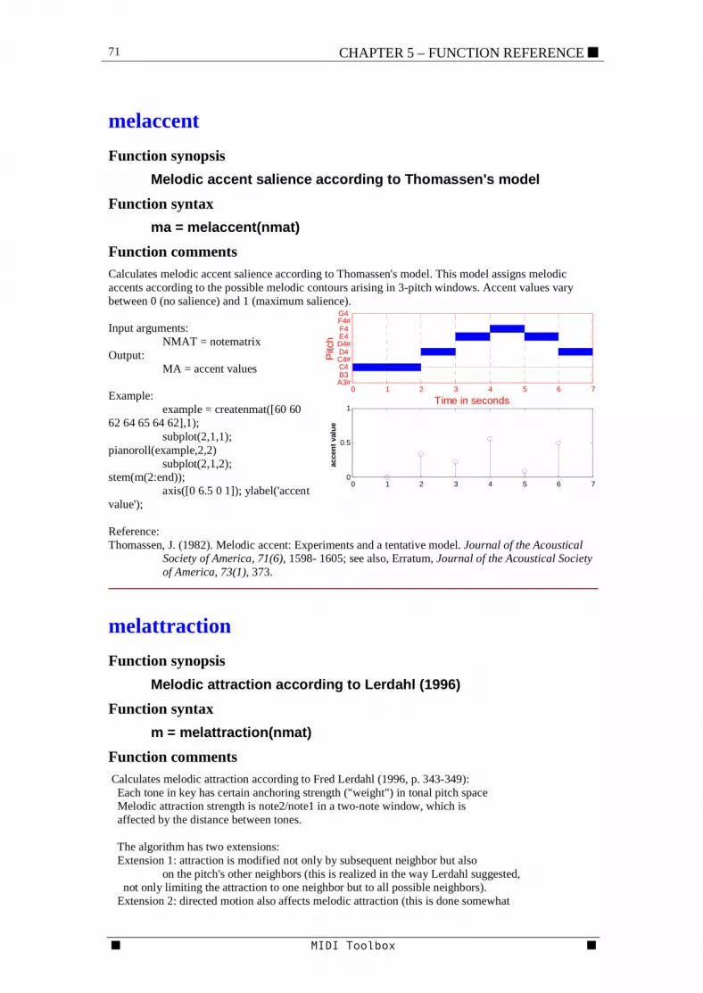
71 CHAPTER 5 – FUNCTION REFERENCE ■
■ MIDI Toolbox ■
0 1 2 3 4 5 6 7A3#B3 C4 C4#D4 D4#E4 F4 F4#G4
Time in seconds
Pitc
h
0 1 2 3 4 5 6 70
0.5
1
acce
nt v
alue
melaccent Function synopsis
Melodic accent salience according to Thomassen's model Function syntax
ma = melaccent(nmat) Function comments Calculates melodic accent salience according to Thomassen's model. This model assigns melodic accents according to the possible melodic contours arising in 3-pitch windows. Accent values vary between 0 (no salience) and 1 (maximum salience). Input arguments: NMAT = notematrix Output: MA = accent values Example: example = createnmat([60 60 62 64 65 64 62],1); subplot(2,1,1); pianoroll(example,2,2) subplot(2,1,2); stem(m(2:end)); axis([0 6.5 0 1]); ylabel('accent value'); Reference: Thomassen, J. (1982). Melodic accent: Experiments and a tentative model. Journal of the Acoustical
Society of America, 71(6), 1598- 1605; see also, Erratum, Journal of the Acoustical Society of America, 73(1), 373.
melattraction Function synopsis
Melodic attraction according to Lerdahl (1996) Function syntax
m = melattraction(nmat) Function comments Calculates melodic attraction according to Fred Lerdahl (1996, p. 343-349): Each tone in key has certain anchoring strength ("weight") in tonal pitch space Melodic attraction strength is note2/note1 in a two-note window, which is affected by the distance between tones. The algorithm has two extensions: Extension 1: attraction is modified not only by subsequent neighbor but also on the pitch's other neighbors (this is realized in the way Lerdahl suggested, not only limiting the attraction to one neighbor but to all possible neighbors). Extension 2: directed motion also affects melodic attraction (this is done somewhat
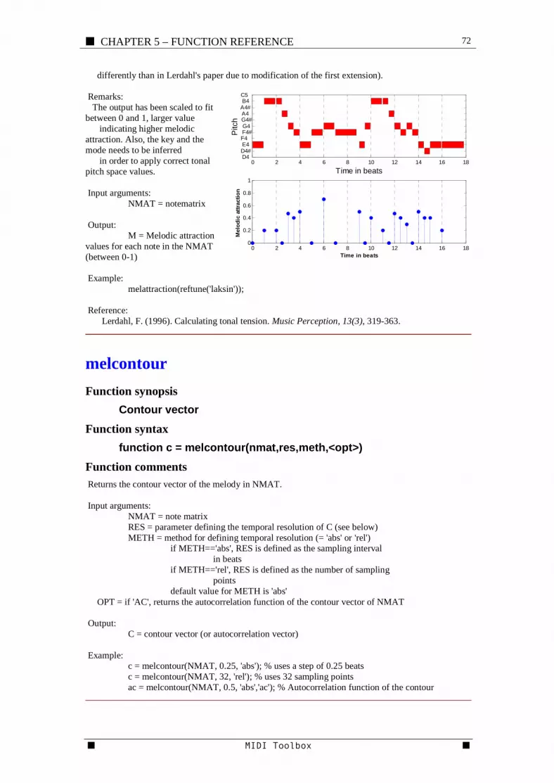
■ CHAPTER 5 – FUNCTION REFERENCE 72
■ MIDI Toolbox ■
0 2 4 6 8 10 12 14 16 18D4 D4#E4 F4 F4#G4 G4#A4 A4#B4 C5
Time in beats
Pitc
h0 2 4 6 8 10 12 14 16 18
0
0.2
0.4
0.6
0.8
1
Mel
odic
attr
actio
n
Time in beats
differently than in Lerdahl's paper due to modification of the first extension). Remarks: The output has been scaled to fit between 0 and 1, larger value indicating higher melodic attraction. Also, the key and the mode needs to be inferred in order to apply correct tonal pitch space values. Input arguments: NMAT = notematrix
Output: M = Melodic attraction values for each note in the NMAT (between 0-1) Example: melattraction(reftune('laksin')); Reference: Lerdahl, F. (1996). Calculating tonal tension. Music Perception, 13(3), 319-363.
melcontour Function synopsis
Contour vector Function syntax
function c = melcontour(nmat,res,meth,<opt>) Function comments Returns the contour vector of the melody in NMAT. Input arguments: NMAT = note matrix RES = parameter defining the temporal resolution of C (see below) METH = method for defining temporal resolution (= 'abs' or 'rel') if METH=='abs', RES is defined as the sampling interval in beats if METH=='rel', RES is defined as the number of sampling points default value for METH is 'abs' OPT = if 'AC', returns the autocorrelation function of the contour vector of NMAT Output: C = contour vector (or autocorrelation vector) Example: c = melcontour(NMAT, 0.25, 'abs'); % uses a step of 0.25 beats c = melcontour(NMAT, 32, 'rel'); % uses 32 sampling points ac = melcontour(NMAT, 0.5, 'abs','ac'); % Autocorrelation function of the contour

73 CHAPTER 5 – FUNCTION REFERENCE ■
■ MIDI Toolbox ■
meldistance Function synopsis
Measurement of distance between two NMATs Function syntax
y=melsim(nmat1,nmat2,<repr>,<metric>,<samples>,<rescale>) Function comments Calculates the similarity of two NMATs in a particular representation. Output is a value indicating distance between nmat1 and nmat2 under the given representation and metric. Output value is rescaled to [0, 1] if rescale is set to 1. Input arguments: NMAT1= first notematrix NMAT2= second notematrix REPR= string denoting the specific representation used for comparison of the two NMATs: 'pcdist1' (default)= distribution of pitch classes 'pcdist2'= distribution of pitch class dyads 'ivdist1'= distribution of intervals 'ivdist2'= distribution of interval dyads 'contour'= melodic contour (input number of samples) 'combcontour'= Combinatorial Contour (does not accept a metric argument) 'durdist1'= distribution of note durations 'durdist2'= distribution of note duration dyads METRIC= string denoting the distance metric used for comparison: 'taxi' (default)=the taxicab norm 'euc'=euclidean distance measure 'cosine' =measure of cosine of the angle between vectors SAMPLES= integer number of samples for contour representation. default value is 10. RESCALE= rescales distance to similarity value between 0 and 1. Default is no rescaling. Set to 1 to rescale values. Output: y = value representing the distance between the two melodies under the given representation and metric. Example: meldistance(nmat1,nmat2,'pcdist1','taxi');
meter Function synopsis
Autocorrelation-based estimate of meter Function syntax
m = meter(nmat,<option>) Function comments Returns an autocorrelation-based estimate of meter of NMAT. Based on temporal structure and on Thomassen's melodic accent.
■ CHAPTER 5 – FUNCTION REFERENCE 74
■ MIDI Toolbox ■
Uses discriminant function derived from a collection of 12000 folk melodies. m = 2 for simple duple m = 3 for simple triple/compound meters (3/8, 3/4, 6/8, 9/8, 12/8, etc.) Input argument: NMAT = notematrix OPTION (Optional, string) = Argument 'OPTIMAL' uses a weighted combination of duration and melodic accents in the inference of meter (see Toiviainen & Eerola, 2004). Input argument: NMAT = notematrix Output: M = estimate of meter (M=2 for duple; M=3 for triple) Reference: Brown, J. (1993). Determination of the meter of musical scores by autocorrelation. Journal of the
Acoustical Society of America, 94(4), 1953-1957. Toiviainen, P. & Eerola, T. (2004). The role of accent periodicities in meter induction: a classification study, In x (Ed.), Proceedings of the ICMPC8 (p. xxx-xxx). xxx:xxx.
meteraccent Function synopsis
Measure of phenomenal accent synchrony Function syntax
a = meteraccent(nmat) Function comments Returns a measure of phenomenal accent synchrony. It consists of durational accents, pitch accents and accentuation from inferred metrical hierarchy. If these accents coincide, accents are highly synchronized. Input arguments: NMAT = notematrix Output: A = integer References: Eerola, T., Himberg, T., Toiviainen, P., & Louhivuori, J. (submitted). Perceived complexity of Western
and African folk melodies by Western and African listeners. Jones, M. R. (1987). Dynamic pattern structure in music: Recent theory and research. Perception and
Psychophysics, 41, 621-634.
See also meter
metrichierarchy Function synopsis
Location of notes in metric hierarchy

75 CHAPTER 5 – FUNCTION REFERENCE ■
■ MIDI Toolbox ■
Function syntax mh = metrichierarchy(nmat)
Function comments Returns a vector indicating the location of each note of NMAT in metric hierarchy. The meter of NMAT is estimated using the function METER. Input argument: NMAT = notematrix Output: MH = vector indicating the location of each note in metric hierarchy; encoding: strong beat = 5, weak beat = 4, etc.
See also meter
midi2hz Function synopsis
Conversion of MIDI note number to frequency (Hz) Function syntax
f = midi2hz(m) Function comments Convert MIDI note numbers to frequencies in Hz. The A3 (Midi number 69) is 440Hz. Input arguments: M = MIDI note numbers Output: F = Frequency in hertz Example: midi2hz(pitch(createnmat));
mobility Function synopsis
Mobility (Hippel, 2000) Function syntax
y= mobility(nmat) Function comments Mobility describes why melodies change direction after large skips by simply observing that they would otherwise run out of the comfortable melodic range. It uses lag-one autocorrelation between successive pitch heights (Hippel, 2000).

■ CHAPTER 5 – FUNCTION REFERENCE 76
■ MIDI Toolbox ■
Input argument: NMAT = notematrix Output: Y = mobility value for each tone in NMAT See also: NARMOUR, TESSITURA Example: y = mobility(nmat) References: von Hippel, P. (2000). Redefining pitch proximity: Tessitura and mobility as constraints on melodic interval size. Music Perception, 17 (3), 315-327.
movewindow Function synopsis
Windowed analysis of notematrix using a specified function Function syntax
y = movewindow(nmat,wlength,wstep,timetype,varargin) Function comments Applies function defined in VARARGIN to a series of windowed note matrices using window length WLENGTH and step WSTEPs across NMAT Input arguments: NMAT = notematrix WLENGTH = window length in seconds WSTEP = window step size in seconds TIMETYPE = time representation, 'beat' (default) or 'sec' VARARGIN = function (string) or functions Output: Y = output of the function VARARGIN (or nested function FUNC2(FUNC1) etc.) applied to NMAT Example 1: Find maximal key correlation within a 3-second window - that is moved by 1.5 seconds at a time - of NMAT y = movewindow(nmat,3,1.5,'sec','maxkkcc'); Example 2: Find average key velocity within a 6-second window - that is moved by 2 seconds at a time - of NMAT y = movewindow(nmat,6,2,'velocity','mean');
narmour Function synopsis
Predictions from Implication-realization model by Narmour (1990) Function syntax
n = narmour(nmat,prin)

77 CHAPTER 5 – FUNCTION REFERENCE ■
■ MIDI Toolbox ■
Function comments Returns the predictions from Implication-realization model of melodic expectancy by Eugene Narmour (1990) Input arguments: NMAT = notematrix PRIN (string) denotes a specific principle: rd = registral direction (revised, Schellenberg 1997) rr = registral return (revised, Schellenberg 1997) id = intervallic difference cl = closure pr = proximity (revised, Schellenberg 1997) co = consonance (Krumhansl, 1995) Output: N = vector for all the tones in NMAT Example: narmour(nmat, 'rd'); References: Narmour, E. 1990. The Analysis and cognition of basic melodic structures: The Implication-realization model. Chicago, IL: University of Chicago Press. Krumhansl, C. L. (1995). Effects of musical context on similarity and expectancy. Systematische musikwissenschaft, 3, 211-250. Schellenberg, E. G. (1997). Simplifying the implication-realization model of melodic expectancy. Music Perception, 14, 295-318.
nmat2snd Function synopsis
Create waveform of NMAT using a simple synthesis Function syntax w = nmat2snd(nmat, <synthtype>,<fs>)
Function comments Create waveform of NMAT using a simple FM synthesis. The default sampling rate is
8192 Hz and velocities are scaled to have a max value of 1. SYNTHTYPE 'fm' (default) uses FM synthesis to approximate horn sound. SYNTHTYPE 'shepard' creates waveform of NMAT using Shepard tones. These tones have also been called 'Circular tones' because they are specifically constructed to contain frequency components at octave intervals with an emphasis of the spectral components between 500Hz and 1000 Hz that effectively eliminates octave information (Shepard, 1964). Part of the code has been obtained from the work of Ed Doering. [email protected] Input argument: NMAT = notematrix SYNTHTYPE (Optional) = Synthesis type, either FM synthesis ('fm', default) or Shepard tones ('shepard') FS (optional) = sampling rate (default 8192)

■ CHAPTER 5 – FUNCTION REFERENCE 78
■ MIDI Toolbox ■
Output: Y = waveform Example 1: samples1 = nmat2snd(laksin); Example 2: samples2 = nmat2snd(laksin,'shepard', 22050); Reference: Moore, F. R. (1990). Elements of Computer Music. New York: Prentice-Hall. Shepard, R. N. (1964). Circularity in judgements of relative pitch. Journal of the Acoustical Society of America, 36, 2346-2353.
nnotes Function synopsis
Number of notes in NMAT Function syntax
n = nnotes(nmat) Function comments Returns the number of notes in NMAT Input argument: NMAT = notematrix Output: N = number of notes in NMAT
notedensity Function synopsis
Number of notes per beat or second Function syntax
n = notedensity(nmat,<timetype>) Function comments Returns the number of notes per beat or second in NMAT Input argument: NMAT = notematrix TIMETYPE (Optional) = timetype ('BEAT' (default) or SEC (Seconds). Output: N = Note density (in beats or seconds) in NMAT

79 CHAPTER 5 – FUNCTION REFERENCE ■
■ MIDI Toolbox ■
notename Function synopsis
Conversion of MIDI numbers to American pitch spelling (text) Function syntax
names = notename(n) Function comments Converts MIDI numbers to American pitch spelling (text) where C4# denotes C sharp in octave 4. Octave 4 goes from middle C up to the B above middle C. Input argument: N = The pitches of NMAT (i.e. pitch(nmat)) Output: text string of equivalent size of N.
See also pianoroll, hz2midi, midi2hz
nPVI Function synopsis
Measure of durational variability of events (Grabe & Low, 2002) Function syntax
function n = nPVI(nmat) Function comments This measure is borne out of language research. It has been noted that the variability of vowel duration is greater in stress- vs. syllable-timed languages (Grabe & Low, 2002). This measure accounts for the variability of durations and is also called "normalized Pairwise Variability Index" (nPVI). Patel & Daniele have applied it to music (2003) by comparing whether the prosody of different languages is also reflected in music. There is a clear difference between a sample of works by French and English composers. Input arguments: NMAT = notematrix Output: N = nPVI index Example: the variability of duration in LAKSIN (a Finnish folk tune available in demos) nPVI(laksin); ans = 26.3861 References: Patel, A. D. & Daniele, J. R. (2003). An empirical comparison of rhythm in language and music. Cognition, 87, B35-B45. Grabe, E., & Low, E. L. (2002). Durational variability in speech and the rhythm class hypothesis. In C. Gussen-hoven & N. Warner, Laboratory phonology (pp. 515-546). 7. Berlin: Mouton de Gruyter.

■ CHAPTER 5 – FUNCTION REFERENCE 80
■ MIDI Toolbox ■
onsetacorr Function synopsis
Autocorrelation function of onset times Function syntax
ac = onsetacorr(nmat, <ndivs>, <fig>,<func>) Function comments Returns autocorrelation of onset times weighted by onset durations. These onset durations, are in turn, weighted by Parncutt's durational accent (1994). This function optionally creates a graph showing the autocorrelation function calculated from onset times weighted by note durations. Finally, a user-defined function (FUNC) can be used to weight the autocorrelation function. For example, TONALITY function is a way of weighting the onset structure by their tonal stability values. MELACCENT may also work in some situations. Input arguments: NMAT = notematrix NDIVS (optional) = divisions per quarter note (default = 4); FIG (optional) = plot figure (yes=1, no=0, default=0) FUNC (optional, string) = Optional function that weights the results, for example 'tonality' function would weight the onsets by their tonal stability values in addition to note durations. Output: AC = values of autocorrelation function between lags 0 ... 8 quarter notes Reference: Brown, J. (1992). Determination of meter of musical scores by autocorrelation. Journal of the acoustical society of America, 94 (4), 1953-1957. Parncutt, R. (1994). A perceptual model of pulse salience and metrical accent in musical rhythms. Music Perception, 11(4), 409-464. Toiviainen, P. & Eerola, T. (2004). The role of accent periodicities in meter induction: a classification study, In x (Ed.), Proceedings of the ICMPC8 (p. xxx-xxx). xxx:xxx.
onsetdist Function synopsis
Distribution of onset times within a measure Function syntax
dist = onsetdist(nmat, nbeats,<fig>) Function comments Returns the distribution of onset times within a measure with a length of NBEATS Input arguments: NMAT = notematrix NBEATS = beats per measure FIG (Optional) = Figure flag (1=figure, 0=no figure)
81 CHAPTER 5 – FUNCTION REFERENCE ■
■ MIDI Toolbox ■
Output: DIST = distribution of onset times
onsetwindow Function synopsis
Onset time based windowing Function syntax
nm = onsetwindow(nmat,mintime,maxtime,<timetype>) Function comments Returns the notes in NMAT whose onset times satisfy MINTIME < onsettime[beats/secs](NMAT) <= MAXTIME Input arguments: NMAT = notematrix MINTIME = minimum limit of the window in beats (default) or secs MAXTIME = maximum limit of the window in beats (default) or secs TIMETYPE = time representation, 'beat' (default) or 'sec' Output: NM = notematrix containing the notes of NMAT whose onsets are within the window
pcdist1 Function synopsis
Pitch-class distribution weighted by note durations Function syntax
pcd = pcdist1(nmat) Function comments Calculates the pitch-class distribution of NMAT weighted by note durations. The note durations are based on duration in seconds that are modified according to Parncutt's durational accent model (1994). Input argument: NMAT = notematrix Output: PCD = 12-component vector listing the probabilities of pitch-classes (C, C#, D, D#, E, F, F#, G, G#, A, A#, B). Example: pcd = pcdist1(nmat)
See also plotdist, refstat , durdist1, durdist2, ivdist1, ivdist2

■ CHAPTER 5 – FUNCTION REFERENCE 82
■ MIDI Toolbox ■
pcdist2 Function synopsis
2nd order pitch-class distribution Function syntax
pcd = pcdist2(nmat) Function comments Calculates the 2nd order pitch-class distribution of NMAT weighted by note durations. The note durations are based on duration in seconds that are modified according to Parncutt's durational accent model (1994). Input argument: NMAT = notematrix Output: PCD = 2nd order pitch-class distribution of NMAT 12 * 12 matrix e.g. PCD(1,2) = probability of transitions from C to C#
See also plotdist, refstat , durdist1, durdist2, ivdist1, ivdist2
perchannel Function synopsis
Channel-by-channel analysis of notematrix using a specified function. Works only with functions returning either scalar or row vector.
Function syntax chout = perchannel(nmat,varargin)
Function comments Channel-by-channel analysis of notematrix using a specified function Input argument: NMAT = note matrix FUNC = function (string) Output: chout = scalar or row vector for each channel. Size depends on the FUNC. Example: p=perchannel(nmat,'pcdist1');
83 CHAPTER 5 – FUNCTION REFERENCE ■
■ MIDI Toolbox ■
See also getmidich, mchannels
pianoroll Function synopsis
Plot pianoroll notation of NMAT Function syntax
pianoroll(nmat,<varargin>) Function comments Plots pianoroll notation of NMAT and takes several optional arguments that affect the information displayed. Input arguments: NMAT = notematrix VARARGIN = various optional input arguments: 'name' = note names for y-axis (default) 'num' = MIDI numbers for y-axis 'beat' = beats for x-axis (default) 'sec' = seconds for x-axis 'vel' = plot note velocities 'mh' = plot metric hierarchy Color parameters, e.g. 'g' = Green pitches in pianoroll 'hold' = current pianoroll is added to a previous figure Output: Figure Remarks: Function displays NMATs with multiple channels using different colors for the different channels. A simple optimization of Y-scale labels is used to increase the legibility of the output. Also, the C notes are marked with dotted line in the plot. Example 1: Plot pitches and their velocities using seconds as the x-axis pianoroll(nmat,'vel','sec'); Example 2: Plot two separate melodies into the same figure pianoroll(nmat1,'r'); % 1st melody in red color pianoroll(nmat2,'b','hold'); % 2nd melody in blue color Example 3: Plot multichannel NMAT (plot channels using different colors) pianoroll(nmat3,'num'); %
playmidi Function synopsis
Creates a temporary MIDI file and plays it using a suitable program
■ CHAPTER 5 – FUNCTION REFERENCE 84
■ MIDI Toolbox ■
Function syntax q = playmidi(nmat,<tempo>)
Function comments Creates a temporary MIDI file and plays it using a suitable program Input argument: NMAT = Notematrix TEMPO (optional)= tempo (default 120 bpm) Output: Opens up MIDI Player and plays temp.mid in the player. Remarks: The player depends on the operating system (Macintosh, PC, Linux). In Windows or MacOS X, the player is defined by definemidiplayer function. Example : playmidi(nmat,145); plays nmat with the tempo 145 beats per minute
playsound Function synopsis
Play NMAT using a simple synthesis Function syntax
q = playsound(nmat) Function comments Create waveform of NMAT using a simple FM synthesis. The default sampling rate is 8192 Hz and velocities are scaled to have a max value of 1 before passing to the fm_synth function. Input argument: NMAT = notematrix SYNTHTYPE (Optional) = Synthesis type, either FM synthesis ('fm', default) or Shepard tones ('shepard') FS (optional) = sampling rate (default 8192) Output: none (played through SOUNDSC) Example 1: playsound(laksin); Example 2: playsound(laksin,'shepard', 22050);
plotdist Function synopsis
Plotting of distributions Function syntax
p = plotdist(dist ,<param>)
85 CHAPTER 5 – FUNCTION REFERENCE ■
■ MIDI Toolbox ■
Function comments This function creates a graph of note-, interval- or duration distributions or transitions. This purpose of the command is make creating simple figures easier. Input arguments: DIST = Distribution of: pitch-classes (12), intervals (25) or durations (9) OR the transitions of the same features; pitch-class transitions (12 x 12), interval transitions (25 x 25), durations transitions (9 x9) or key correlations (24), interval sizes (1x13) or intervals directions (1x12). For the last one, % a simple heuristic is used to distinguish it from the pitch-class distribution. PARAM (optional) = color parameters (e.g. 'k' for black bars or [.1 .4 .9] for specific colors). For transition plots, use 'hot' or other colormap definition. Default color is gray in both cases. Output: Figure Remarks: The distribution needs to be calculated separately. Example: Create note transition figure of laksin MIDI file plotdist(pcdist2(laksin))
plothierarchy Function synopsis
Plot metrical hierarchy Function syntax
fig = plothierarchy(nmat) Function comments Plots metrical hierarchy based on meter-finding and assigning metrical grid to each note according to its position in the grid. Lerdahl & Jackendoff (1983). Input argument: NMAT = notematrix Output: FIG = Figure Reference: Lerdahl, F., & Jackendoff, R. (1983). A generative theory of tonal music. Cambridge, MA: MIT Press.
■ CHAPTER 5 – FUNCTION REFERENCE 86
■ MIDI Toolbox ■
plotmelcontour Function synopsis
Plot melodic contour using STEP resolution Function syntax
p = plotmelcontour(nmat,<step>,<meth>,<options>) Function comments Plot melodic contour using a user-defined resolution. Various other output options can be used (VARARGIN). Input argument: NMAT = notematrix VARARGIN = Various other parameters: STEP (numeric) = resolution (optional), see 'abs' or 'rel' below: 'abs' defines the sampling interval in beats (default) rel' defines the number of sampling points 'beat' (default) defines the timetype in beats 'sec' defines the timetype in seconds COLOR OPTIONS, e.g., 'r:' for red, dotted line... (optional) 'ac' for autocorrelation figure (optional). This option plots the contour self-similarity of NMAT. The similarity is based on autocorrelation, where the melodic contour is correlated with a copy of itself. A short duration (approximately one measure) from the beginning is left out in the plot. Output: P = Figure Example 1: plot melodic contour plotmelcontour(laksin,0.1,'abs',':ok'); Example 2: plot contour self-similarity plotmelcontour(laksin,0.1,'abs','r','ac');
See also melcontour
quantize Function synopsis
Quantize note onsets and durations of NMAT Function syntax
nm2= quantize(nmat, onsetres, <durres>, <filterres> ) Function comments Quantize note events in NMAT according to onset resolution (ONSETRES), durations resolution (DURRES) and optionally filter note events shorter than the filter threshold (FILTERRES). Input arguments: NMAT = notematrix

87 CHAPTER 5 – FUNCTION REFERENCE ■
■ MIDI Toolbox ■
ONSETRES = onset threshold for quantization (e.g., quarter note = 1/4). Default value is 1/8 note. DURRES (optional) = duration threshold for quantization. Default is double the value of ONSETRES. FILTERRES (optional) = duration threshold for filtering out notes. For example, to filter out eight notes and shorter notes events, FILTERRES of 1/8 can be used. Output: NM2 = quantized notematrix Example: Quantize NMAT to quarter notes (onsets and durations) and filter out all notes shorter than 1/8 beats nm2 = quantize(nmat, 1/4, 1/4,1/8);
readmidi Function synopsis
Conversion of MIDI file to notematrix Function syntax
nmat = readmidi(fn) Function comments Input argument: FN = name of the MIDI file (string) Output: NMAT = notematrix
See also writemidi
refstat Function synopsis
Returns reference statistic of melody and associated labels specified by STAT
Function syntax [ref, label] = refstat(stat)
Function comments REFSTAT function returns a selected reference statistic of melody (STAT): Input arguments: STAT= any of the following strings: kkmaj = Krumhansl & Kessler (1982) major key profile (tonality) kkmin = Krumhansl & Kessler (1982) minor key profile (tonality) kkmajt = Krumhansl & Kessler (1982) major key profile modified by Temperley (1999) kkmint = Krumhansl & Kessler (1982) minor key profile modified by Temperley (1999)
■ CHAPTER 5 – FUNCTION REFERENCE 88
■ MIDI Toolbox ■
pc_all = Pitch-Classes in the Essen Collection (ALL songs, incl. Asian) by Schaffrath (1995) pc_europe_maj = Pitch-classes in Essen Collection (Major songs, not incl. Asian) pc_europe_min = Pitch-classes in Essen Collection (Minor songs, not incl. Asian) iv_all = Intervals from Essen folksong collection ivnd_europe = Intervals (no direction) from Essen col., not incl. Asian) ivudr_europe = Intervals (up, down, repeat) Essen col., not incl. Asian) iv_europe_maj = Interval transitions (Essen col., Major, Non-Asian) ivdia_europe = Interval transitions, diatonic only (Essen col., not incl. Asian) ivdiand_europe = Interval transitions, diatonic only, no direction (Essen col., not incl. Asian) iv2 = Interval transitions (From Essen folksong collection) (VECTOR) twotone = Pitch-class transitions in Essen Collection (VECTOR) pcdist1essen = Pitch-classen in Essen Collection (All songs, not incl. Asian, N=6231) ivdist1essen = Intervals from Essen folksong collection (not incl. Asian) durdist1essen = Duration distribution (From Essen folksong collection) ivdist2essen = Interval transitions (From Essen folksong collection) (MATRIX) pcdist2essen = Pitch-class transitions (From Essen folksong collection) (MATRIX) durdist2essen = Duration transitions (From Essen folksong collection) (MATRIX) pcdist2classical1 = Tone-transition probabilities from 16000 + classical music themes (Simonton, 1984) pcdist2classical2 = Frequency of occurrence of melodic intervals by Youngblood (1958) pcdist1schubert = Pitch-class distribution in Schubert pieces (Major key, Knopoff & Hutchinson (1983) Output: REF = probability vector for each component in the statistic. For example, major key profile is: ref=[6.35,2.23,3.48,2.33,4.38,4.09,2.52,5.19,2.39,3.66,2.29,2.88]; LABEL = label for each statistic. As above this, would output: 'C','C#','D','D#','E','F','F#','G','G#','A','A#','B' References: Knopoff, L. & Hutchinson, W. (1983). Entropy as a measure of style: The influence of sample length. Journal of Music Theory, 27, 75-97. Krumhansl, C. L., & Kessler, E. J. (1982). Tracing the dynamic changes in perceived tonal organization in a spatial representation of musical keys. Psychological Review, 89, 334-368. Schaffrath, H. (1995). The Essen Folksong Collection in Kern Format. [computer database] D. Huron (Ed.). Menlo Park, CA: Center for Computer Assisted Research in the Humanities. Simonton, D. K. (1984). Melodic structure and note transition probabilities: A content analysis of 15,618 classical themes. Psychology of Music, 12, 3-16. Temperley, D. (1999). What's Key for Key? The Krumhansl-Schmuckler key-finding algorithm reconsidered. Music Perception, 17, 65-100. Youngblood, J.E. (1958). Style as information. Journal of Music Theory, 2, 24-35. Example 1: Get major key profile by Krumshansl & Kessler (1982): major = refstat('kkmaj'); Example 2: Get interval transition probabilities in the Essen collection and the respective labels for all interval transitions: [inttrans,label] = refstat('ivdist2essen');
reftune Function synopsis
Obtain a 'reference' or example tune
89 CHAPTER 5 – FUNCTION REFERENCE ■
■ MIDI Toolbox ■
Function syntax nmat = reftune('name',<dur>)
Function comments Input arguments: NAME= any of the following strings: dowling1 = Dowling (1973) tune 1 dowling1 = Dowling (1973) tune 2 int1-12 = Hartmann & Johnson (1991) tunes 1-12 probe = Sample probe sequence (demonstrated in the Manual) tritone = 12 random tritone intervals demonstrating the Tritone Paradox (Deutsch, 1991) laksin = Two phrases of a Finnish Folk, "Läksin Minä Kesäyönä" DUR(optional) = duration of tones in target NAME tune Output: NMAT = the sequence as a notematrix References: Dowling, W. J. (1973). The perception of interleaved melodies, Cognitive Psychology,5, 322-337. Hartmann, W. M., & Johnson, D. (1991). Stream segregation and peripheral channeling. Music Perception, 9(2), 155-184. Deutsch, D. (1991). The tritone paradox: An influence of language on music perception. Music Perception, 8, 335-347. Repp, B. (1994). The tritone paradox and the pitch range of the speaking voice: A dubious connection. Music Perception, 12, 227-255.
scale Function synopsis
Scaling of notematrix values Function syntax
nm = scale(nmat,dim,factor) Function comments Scales note data in given dimension (time, onset time, or duration) Input arguments: NMAT = notematrix DIM = dimension ('time', 'onset', 'dur' or 'vel') FACTOR = amount of scale (must be > 0) Output: NM = notematrix containing the scaled version of NMAT Examples: nm = scale(nmat,'time',2); % scales time axis by a factor of 2 nm = scale(nmat,'dur',0.5); % shortens durations by a factor of 2

■ CHAPTER 5 – FUNCTION REFERENCE 90
■ MIDI Toolbox ■
segmentgestalt Function synopsis
Segmentation algorithm by Tenney & Polansky (1980) Function syntax
[c,s] = segmentgestalt (nmat ,<fig>) Function comments Input arguments: NMAT = notematrix FIGURE (optional) = if any second argument given, a figure is plotted Output: C = clang boundaries (binary (0|1) column vector) S = segment boundaries (binary (0|1) column vector) FIG (optionally) = plot pianoroll with dotted lines corresponding with clang boundaries. Solid line indicates segment boundaries. References: Tenney, J. & Polansky, L. (1980). Temporal gestalt perception in music. Journal of Music Theory, 24(2), 205–41.
See also segmentprob
segmentprob Function synopsis
Estimation of segment boundaries Function syntax
segmentprob(nmat , <thres>,<fig>) Function comments Plots a segmentation of NMAT based on Markov probabilities of segment boundaries derived from the Essen collection Input arguments: NMAT = notematrix THRES (optional) = segmentation threshold (default = 0.6); FIG (optional) = plot figure (yes=1, no=0, default=0) Output: SEGM = Segment probabilities for note event (row vector) Figure (Optional) showing the pianoroll notation of NMAT in top and estimated segment boundaries with respective probabilities as a stem plot.
See also segmentgestalt

91 CHAPTER 5 – FUNCTION REFERENCE ■
■ MIDI Toolbox ■
setmidiplayer Function synopsis
midiplayer = setmidiplayer(<fullpath>) Function syntax
Define MIDI player program in Windows Function comments midiplayer = setmidiplayer(<fullpath>); Input argument: FULLPATH (optional) = define the full path of your player Remarks: Used by the PLAY function. Example : midiplayer = setmidiplayer('C:\Program Files\ ... Windows Media Player\mplayer2.exe');
settempo Function synopsis
Assigns a new tempo to the NMAT in beats per minute (BPM) Function syntax
y = settempo(nmat,bpm) Function comments Assigns a new tempo to the NMAT. Input argument: NMAT = notematrix BPM = new tempo (in beats per minute) Output: NMATF = new notematrix
See also gettempo
setvalues Function synopsis
Sets the chosen notematrix value for every event

■ CHAPTER 5 – FUNCTION REFERENCE 92
■ MIDI Toolbox ■
Function syntax nm = setvalues(nmat,dim,val,<timetype>)
Function comments Sets the chosen notematrix value for every event Input arguments: NMAT = notematrix DIM = dimension ('onset', 'dur', 'vel', or 'chan') VAL = Value TIMETYPE = (optional) time representation, 'beat' (default) or 'sec' Output: NM = notematrix containing the scaled version of NMAT Examples: nm = setvalues(nmat,'vel',64); % Sets all note velocities to 64 nm = setvalues(nmat,'onset',0); % Sets all onset times to zero nm = setvalues(nmat,'dur',1,'sec'); % Sets all note durations to 1 sec
shift Function synopsis
Shifting of notematrix values Function syntax
nm = shift(nmat,dim,amount,<timetype>) Function comments Shifts note data in given dimension (onset time, duration, or pitch) Input arguments: NMAT = notematrix DIM = dimension ('onset', 'dur', 'pitch', 'chan' or 'vel') AMOUNT = amount of shift TIMETYPE = (optional) time representation, 'beat' (default) or 'sec' Output: NM = notematrix containing the shifted version of NMAT Examples: nm = shift(nmat,'onset',5); % shifts note onsets 5 beats ahead nm = shift(nmat,'dur',-0.1,'sec'); % shortens durations by 0.1 secs nm = shift(nmat,'pitch',12); %transposes one octave up
tessitura Function synopsis
Tessitura (Hippel, 2000)
93 CHAPTER 5 – FUNCTION REFERENCE ■
■ MIDI Toolbox ■
Function syntax y = tessitura(nmat)
Function comments Calculates the tessitura that is based on standard deviation of pitch height. The median range of the melody tends to be favored and thus more expected. Tessitura predicts whether listeners expect tones close to median pitch height (Hippel, 2000). Input argument: NMAT = notematrix Output: Y = tessitura value for each tone in NMAT Example: y = tessitura(nmat) References: von Hippel, P. (2000). Redefining pitch proximity: Tessitura and mobility as constraints on melodic interval size. Music Perception, 17 (3), 315-327.
See also mobility, narmour
tonality Function synopsis
Tonal stability of notes in melody Function syntax
p = tonality(nmat) Function comments Function gives the tonal stability ratings for tones in the melody (NMAT) after determining the key mode (minor/major) using the KEYMODE function. Input argument: NMAT = notematrix Output: P = tonality values for pitches in NMAT Remarks: This function calls the KEYMODE function. Reference: Krumhansl, C. L. (1990). Cognitive Foundations of Musical Pitch. New York: Oxford University Press. Example: p = tonality(createnmat)

■ CHAPTER 5 – FUNCTION REFERENCE 94
■ MIDI Toolbox ■
See also refstat, keymode
transpose2c Function synopsis
Transposition to C tonic Function syntax
nmatf = transpose2c(nmat) Function comments Transposes NMAT to C major or minor using the Krumhansl-Kessler algorithm. Note that the algorithm may not give reliable results if the NMAT is especially short or has a modulating structure. Input argument: NMAT = notematrix Output: NMATF = transposed notematrix Example: n = transpose2c(nmat);
trim Function synopsis
Removal of leading silence Function syntax
nm2 = trim(nmat) Function comments Removes potential silence in the beginning of NMAT by shifting the note onsets so that the first onset occur at zero time Input arguments: NMAT = notematrix
writemidi Function synopsis
Writes a MIDI file from a NMAT Function syntax
n = writemidi(nmat, ofname, <tpq>, <tempo>, <tsig1>, <tsig2>)

95 CHAPTER 5 – FUNCTION REFERENCE ■
■ MIDI Toolbox ■
Function comments Creates a MIDI file from a NMAT using various optional parameters Input arguments: NMAT = notematrix OFNAME = Output filename (*.mid) TPQ (Optional) = Ticks per quarter note (default 120) TEMPO (Optional) = bpm, beats per minute (default 100) TSIG1&2 (Optional) = Time-signature, e.g. 6/8 -> TSIG1 = 6, TSIG2 = 8 (default 4) Output: MIDI file Remarks: TEXT2MIDI converter needs to be handled differently in PC and Mac. Example: writemidi(a,'demo.mid'); creates a file name DEMO.MID from notematrix A with default settings.
■ CHAPTER 5 – FUNCTION REFERENCE 96
■ MIDI Toolbox ■
Alphabetical Index of Functions ambitus ...................................53 analyzecoll..............................53 analyzedir...............................53 boundary ................................54 combcontour ..........................55 complebm ...............................55 compltrans .............................56 concur .....................................56 createnmat .............................57 dir2coll....................................58 dropmidich.............................58 dropshortnotes.......................58 duraccent................................59 durdist1 ..................................59 durdist2 ..................................60 elim .........................................60 entropy ...................................61 extreme...................................61 filtercoll ..................................62 getmidich................................62 gettempo.................................63 gradus.....................................63 hz2midi ...................................63 ismonophonic .........................64 ivdist1 .....................................64 ivdist2 .....................................65 ivdirdist1 ................................65
ivsizedist1 .............................. 66 keymode................................. 66 keyname................................. 67 keysom ................................... 67 keysomanim........................... 68 kkcc ........................................ 69 kkkey...................................... 69 maxkkcc................................. 70 mchannels.............................. 70 melaccent ............................... 71 melattraction......................... 71 melcontour............................. 72 meldistance............................ 73 meter ...................................... 73 meteraccent ........................... 74 metrichierarchy .................... 74 midi2hz .................................. 75 mobility.................................. 75 movewindow.......................... 76 narmour................................. 76 nmat2snd ............................... 77 nnotes..................................... 78 notedensity............................. 78 notename ............................... 79 nPVI....................................... 79 onsetacorr.............................. 80 onsetdist ................................. 80
onsetwindow .......................... 81 pcdist1 .................................... 81 pcdist2 .................................... 82 perchannel ............................. 82 pianoroll................................. 83 playmidi ................................. 83 playsound............................... 84 plotdist ................................... 84 plothierarchy ......................... 85 plotmelcontour ...................... 86 quantize.................................. 86 readmidi................................. 87 refstat ..................................... 87 reftune.................................... 88 scale ........................................ 89 segmentgestalt ....................... 90 segmentprob .......................... 90 setmidiplayer ......................... 91 settempo ................................. 91 setvalues ................................. 91 shift......................................... 92 tessitura.................................. 92 tonality ................................... 93 transpose2c ............................ 94 trim......................................... 94 writemidi................................ 94
Copyright © 2022 FDOKUMEN