BioMed CentralBMC Neuroscience

ss

Open AcceSoftwareBump time-frequency toolbox: a toolbox for time-frequency oscillatory bursts extraction in electrophysiological signalsFrançois B Vialatte*1, Jordi Solé-Casals2, Justin Dauwels3, Monique Maurice1 and Andrzej Cichocki1

Address: 1Riken BSI, Lab. ABSP, Wako-Shi, Japan, 2University of Vic, Vic, Spain and 3MIT, Cambridge, MA, USA

Email: François B Vialatte* - fvialatte@brain.riken.jp; Jordi Solé-Casals - jordi.sole@uvic.es; Justin Dauwels - jdauwels@mit.edu; Monique Maurice - mvialatte@brain.riken.jp; Andrzej Cichocki - cia@brain.riken.jp

* Corresponding author

AbstractBackground: oscillatory activity, which can be separated in background and oscillatory burstpattern activities, is supposed to be representative of local synchronies of neural assemblies.Oscillatory burst events should consequently play a specific functional role, distinct frombackground EEG activity – especially for cognitive tasks (e.g. working memory tasks), bindingmechanisms and perceptual dynamics (e.g. visual binding), or in clinical contexts (e.g. effects of braindisorders). However extracting oscillatory events in single trials, with a reliable and consistentmethod, is not a simple task.

Results: in this work we propose a user-friendly stand-alone toolbox, which models in areasonable time a bump time-frequency model from the wavelet representations of a set of signals.The software is provided with a Matlab toolbox which can compute wavelet representations beforecalling automatically the stand-alone application.

Conclusion: The tool is publicly available as a freeware at the address: http://www.bsp.brain.riken.jp/bumptoolbox/toolbox_home.html

BackgroundThe structural organization (which elements are relevant)and associated functional role (how these elements play arole in brain dynamics) of electroencephalographic (EEG)oscillations are still far from being completely under-stood. Oscillatory activity can be separated in background(or ongoing) and transient burst pattern activities. Thebackground EEG is constituted by regular waves, whereasbursts are transient and with higher amplitudes: corticaldynamics do not follow continuous patterns, but insteadoperates in steps, or frames [1]. These bursts are organized

local activities, most likely to be representative of localsynchronies. Synchrony among oscillating neural assem-blies is a plausible candidate to mediate functional con-nectivity, and therefore to allow the formation ofspatiotemporal representations [2,3]. Oscillatory burstsshould consequently play a specific functional role, dis-tinct from ongoing background EEG activity (which doesnot mean however that background activity cannot con-vey information). They are correlated with reciprocaldynamic connections of neural structures, which can beconsidered as distributed local networks of neurons [4].

Published: 12 May 2009

BMC Neuroscience 2009, 10:46 doi:10.1186/1471-2202-10-46

Received: 6 November 2008Accepted: 12 May 2009

This article is available from: http://www.biomedcentral.com/1471-2202/10/46

© 2009 Vialatte et al; licensee BioMed Central Ltd. This is an Open Access article distributed under the terms of the Creative Commons Attribution License (http://creativecommons.org/licenses/by/2.0), which permits unrestricted use, distribution, and reproduction in any medium, provided the original work is properly cited.

Page 1 of 12(page number not for citation purposes)

BMC Neuroscience 2009, 10:46 http://www.biomedcentral.com/1471-2202/10/46

Together, distant neural assemblies are involved in collec-tive dynamics of synchronous neuronal oscillations [3],taking the shape of oscillatory patterns.

EEG activities are usually analyzed using either time or fre-quency representations of event related potentials (ERP),which can be interpreted as the reorganization of thespontaneous brain oscillations in response to the stimu-lus [5,6]. ERP can be further seprated into two sub-groups:event related synchronization (ERS), and similarly eventrelated desynchronization (ERD). The simplest hypothe-sis concerning the origins of ERP would be additive: fol-lowing the stimulus onset, in each trial, a transient changeof amplitude is observed in a given frequency range, inde-pendent of the ongoing signal (the signal is synchronizedor dissynchronized in all trials). However, other compet-ing theories could also explain the ERP patterns. The stim-ulus could induce a change in the phase of ongoingoscillations, without power changes. If the phases of alltrials were aligned or dialigned, then after averaging ongo-ing oscillations an ERS or ERD pattern would arise: this isthe so-called theory of phase resetting (e.g. [7,8]; see also[9]). Another recent theory explains the generation ofevent related potentials as a consequence of a baselineshift of ongoing activity [10]. Confronting these threecompeting theories with experimental facts seems neces-sary in order to understand the basis of neural dynamics.

It should be noted however that all the above ERP theoriesare interested in the study of averages of electrophysiolog-ical signals in the time domain. ERP were observed in sev-eral studies to have visible outcomes even in single trials[11,12], especially observable when using wavelets[6,12,13] which represent the signal with optimal time-frequency resolutions. Local oscillatory events are presentin single trials, appearing as transient oscillatory synchro-nizations (TOS) or transient oscillatory desynchroniza-tions (TOD), corresponding to the presence or absence ofa coherent neural assembly [6]. If the additive theory wasright, ERS and ERD could be assumed to be the outcomeof an average of TOS and TOD events respectively – if not(especially in the phase shift theory), they would have anindependent meaning, and it would be even more worth-wile to study them. We are not interested here in an aver-aged outcome (we do not want to study ERP, but TOS andTOD), because the brain itself usually processes informa-tion in single trials.

Instead of using average approaches, one could try to ana-lyze directly single trials in the time-frequency plane.However, in the case of time-frequency planes, hundredsof thousands of coefficients are used to represent a signal;and when a large set of signals is to be compared, the com-plexity of simple graphical matching methods becomesintractable. Analyzing directly this large amount of infor-

mation leads to complex computations, and eitherapproximate or over-fitted models (this problem is usu-ally termed as the "curse of dimensionality"). We insteadadvocate a sparsification approach. The main purpose ofsparsification approaches is to extract relevant informa-tion within redundant data. Sparse time-frequency bumpmodeling, a 2D extension of the 1D bump modelingdescribed in [14], was developed for this purpose: sparsetime-frequency bump modeling extracts the most promi-nent bursts within a normalized time-frequency map, bymodeling them into a sum of parametric functions (seeFig. 1). Bump modeling is however not the only possiblesparsification approach. The ridges [15,16] of waveletmaps can be extracted; but while they are sparse, their bio-logical interpretation is not trivial. Multiway analysis [17]allows the simultaneous extraction of multi-dimensionalmodes, and can be applied to time-frequency representa-tions of electrophysiological signals (e.g. [18]); however itdoes not allow the independent analysis of transient oscil-lations. Wavelet packets [16,19] allow the computation ofvery sparse time-frequency representation (which can beefficient for signal compression, sometimes also for fea-ture extraction); however, because they provide inaccuratetime-frequency locations of oscillatory contents, the useof discrete wavelets is not appropriate for signal analysis –especially for electrophysiological data. Finally, the clos-est method to bump modeling would be matching pursuit[20], which associates a library of functions to a signal –the signal is thereby decomposed into a set of atomicfunctions, each with specific time-frequency properties(one function could be used to represent a transient oscil-lation). Other more straightforward attempts were alsomade at extracting specific atoms of EEG oscillations, likefor instance the extraction of narrow band alpha peakepochs [9], or the analysis of a specific time-frequencyarea (e.g. [21]), but with limitations due to an a prioridefined time-frequency area or frequency range [22]. As acomparison, sparse bump modeling allows an automaticbroadband modeling of time-frequency atoms, each ofthem interpreted as transient local activities of neuralassemblies (TOS or TOD).

Sparse time-frequency bump modeling was first appliedto model invasive EEG (local field potentials), recordedfrom rats olfactory bulb during a go-no go olfactory mem-ory task [22,23]. Afterwards, it was used to investigate sev-eral aspects of brain oscillatory dynamics: scalp EEG datafrom patients with early stage of Alzheimer's disease (AD)was also successfully analyzed and classified using bumpmodeling [22,24,25] with a high accuracy (80–93% leave-one-out validation rate). The model was also applied torepresent simultaneously time-frequency and space infor-mation using a sonification approach [26]. Time-fre-quency space information was then exploited using asynchrony model: oscillatory burst extracted with bump

Page 2 of 12(page number not for citation purposes)

BMC Neuroscience 2009, 10:46 http://www.biomedcentral.com/1471-2202/10/46

Page 3 of 12(page number not for citation purposes)

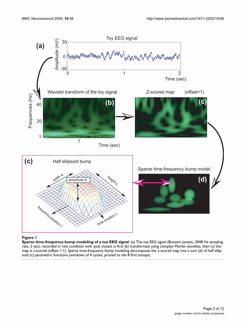
Sparse time-frequency bump modeling of a toy EEG signalFigure 1Sparse time-frequency bump modeling of a toy EEG signal. (a) The toy EEG signal (Biosemi system, 2048 Hz sampling rate, 2 sec), recorded in rest condition with eyes closed, is first (b) transformed using complex Morlet wavelets, then (c) the map is z-scored (offset = 1). Sparse time-frequency bump modeling decomposes the z-scored map into a sum (d) of half ellip-soid (c) parametric functions (windows of 4 cycles, pruned to the 8 first bumps).

-30

30

0

1 20Time (sec)

Am

plitu

de (m

V) Toy EEG signal

1

20

40

1

Freq

uenc

ies

(Hz)

Time (sec)

Wavelet transform Z-scored map

Sparse time-frequency

time position t

frequency position f

height hwidth w

Half ellipsoid bump

amplitude A

(offset=1)

bump model

of the toy signal

(a)

(b) (c)

(c)

(d)

BMC Neuroscience 2009, 10:46 http://www.biomedcentral.com/1471-2202/10/46

modeling were used to determine large-scale synchrony –the stochastic event synchrony (SES, [27,28]). Applied toEEG recorded from early AD patients, SES extracted signif-icant differences with age-matched control subjects. Thesedifferences were complementary when compared against30 other synchrony measures [29,30] (uncorrelated withall other 30 measures). Finally, oscillations of steady statevisual event potential epochs were extracted (hundred sin-gle trial EEG signals) using sparse bump modeling, and anincrease of large-scale synchrony measured using SES[31]. This confirms that sparse bump modeling has a widerange of possible applications, from feature extraction tosignal modeling and analysis.

However, due to its complexity, it was until now difficultfor researchers to reproduce our results: only one externalgroup [32] tried to reproduce results obtained with bumpmodeling on Alzheimer's disease modeling (theyobtained an 80% classification rate). Therefore we presentnow a toolbox [see Additional file 1] for sparse bumpmodeling. The software extracts transient oscillatoryevents (TOS or TOD). We will first describe the methodprocedure, then demonstrate the toolbox functions with atoy signal. In appendix, we present some details of theimproved adaptation and matching methods imple-mented in the toolbox.

ImplementationMethod ProcedureButIf toolbox follows four steps (rationales for this proce-dure, proofs and technical details are explained in [22],see also Fig. 1): (in Matlab) the signal is first wavelet trans-formed into time-frequency, then the time-frequency mapis z-score normalized; (in the stand-alone software) themap is described by a set of time-frequency window, thenparametric functions are adapted within these windows,in decreasing ordered of energy.

The first steps are executed with Matlab, while the last areexecuted with a stand-alone software. Note however thatthe stand-alone software can be directly called by Matlab:the whole package can be run from Matlab.

WaveletsWavelets (see [16,19] for details), especially complexMorlet wavelets [33], have already been widely used fortime-frequency analysis of EEG signals [13,34-39]. Com-plex Morlet wavelets ϑ of Gaussian shape in time (devia-tion σ) are defined as:

where σ and f are interdependent parameters, the con-straint 2πft > 5. The wavelet family defined by 2πft = 7, asdescribed in [34], is adapted to the investigation of EEGsignals. This wavelet has positive and negative valuesresembling those of an EEG, but also a symmetric Gaus-sian shape both in the time and frequency domains – i.e.this wavelet locates accurately time-frequency oscillationsboth in the time and frequency domain.

We scale complex Morlet wavelet ϑ to compute time-fre-quency wavelet representations of the signal X of length T:

where s, the scaling factor, controls the central frequency fof the mother wavelet. The modulus of this time-scale rep-resentation can therefore be used as a positive time-fre-quency spectrogram, which we will note Cx, a time-frequency matrix of dimension T × F, where F scales areused to compute appropriate frequency steps (usually lin-ear or logarithmic, in the case of bump modeling we uselinear steps).

Z-scoreThe time-frequency spectrogram is normalized dependingon a reference signal. The reference signal is used to deter-mine the usual distribution of the time-frequency map:bump modeling will extract activities with transientamplitudes above or below this usual distribution (i.e.high or low z-score). The reference signal R of dimensionU is wavelet transformed into a spectrogram Cr of dimen-sion U × F. The average Mf(Cr) = [μ1(Cr), μ2(Cr),..., μF(Cr)]and standard deviations Sf(Cr) = [σ1(Cr), σ2(Cr),..σF(Cr)]are computed from Cr for each of the F frequencies of thematrix Cr. For instance, at frequency i:

and

The z-scored map Zx is obtained through normalization ofthe wavelet map Cx using these values:

In event related studies, the reference signal is usually asignal recorded during a rest period, just before the stim-ulus period (the so-called pre-stimulus period). In rest

ϑ σ π( ) . . ,t A e

t

e i ft=

− 2

2 2 2(1)

(2)C t st

sdx

T( , ) ( ) * ,= −⎛

⎝⎜⎞⎠⎟∫ X τ ϑ τ τ

μ i

t itU

U( )

( , ),C

Crr = =∑ 1 (3)

σμ

i

t i itU

U( )

( ( , ) ( )).C

Cr Crr =

−=∑ 21 (4)

ZCx Cr

Crx( , )

( , ) ( )

( ).f t

f t f

f=

−μσ

(5)

Page 4 of 12(page number not for citation purposes)

BMC Neuroscience 2009, 10:46 http://www.biomedcentral.com/1471-2202/10/46

condition, the reference signal can be either the signalitself (self-reference signal); or a statistic derived from agroup of signals (as used e.g. in [26]). The minimalnumber of samples of the reference signal should bedetermined with regards to the lowest frequency range(because low frequencies have longer cycles than high fre-quencies), so that a sufficient number of cycles is present– otherwise, the reference statistic would not be signifi-cant.

WindowingThe z-scored map is analyzed in a time-frequency area ofinterest defined by the user, with lowest frequency fm andhighest frequency fx. The z-scored map Zx is described bya set of windows ω(f, t) with f ∈ [fm, fm + 1,...fx], t ∈ [bt, bt+ 1...T - bt] the position on the general time-frequencymap respectively in frequency and time. Each ω has itsown dimensions H × W (height and width), determineddepending on the time-frequency resolution at the win-dow's central frequency. The dimension W is determinedto have a duration of a fixed (usually 4) number of cycles(for instance, W = 1 sec. for activities with central fre-quency at 4 Hz, W = 100 msec. for activities at 40 Hz). Thedimension H is determined as the ratio of W to the time-frequency resolution (see [22]). The limit bt is determinedso that bt = W/2 for the windows at the frequency fm (lowfrequency windows are larger than high frequency win-dows). In other words, the left and right limits of the mod-eled area are vertical, and constrained by the lowerfrequency so as to allow the modelisation of bumps cen-tered at these limits [22] (similarly, the z-score map ismodelled with extract upper and lower borders in fre-quencies).

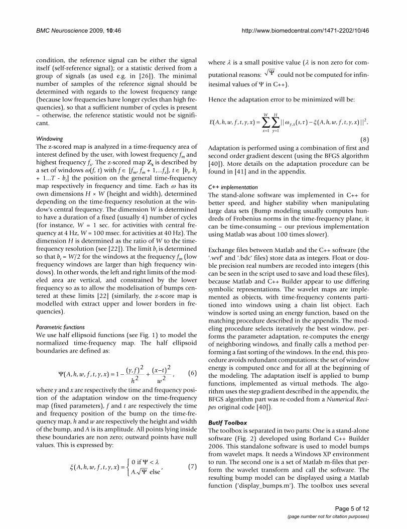
Parametric functionsWe use half ellipsoid functions (see Fig. 1) to model thenormalized time-frequency map. The half ellipsoidboundaries are defined as:

where y and x are respectively the time and frequency posi-tion of the adaptation window on the time-frequencymap (fixed parameters), f and t are respectively the timeand frequency position of the bump on the time-fre-quency map, h and w are respectively the height and widthof the bump, and A is its amplitude. All points lying insidethese boundaries are non zero; outward points have nullvalues. This is expressed by:

where λ is a small positive value (λ is non zero for com-

putational reasons: could not be computed for infin-

itesimal values of Ψ in C++).

Hence the adaptation error to be minimized will be:

Adaptation is performed using a combination of first andsecond order gradient descent (using the BFGS algorithm[40]). More details on the adaptation procedure can befound in [41] and in the appendix.

C++ implementationThe stand-alone software was implemented in C++ forbetter speed, and higher stability when manipulatinglarge data sets (Bump modeling usually computes hun-dreds of Frobenius norms in the time-frequency plane, itcan be time-consuming – our previous implementationusing Matlab was about 100 times slower).

Exchange files between Matlab and the C++ software (the'.wvf' and '.bdc' files) store data as integers. Float or dou-ble precision real numbers are recoded into integers (thiscan be seen in the script used to save and load these files),because Matlab and C++ Builder appear to use differingsymbolic representations. The wavelet maps are imple-mented as objects, with time-frequency contents parti-tioned into windows using a chain list object. Eachwindow is sorted using an energy function, based on thematching procedure described in the appendix. The mod-eling procedure selects iteratively the best window, per-forms the parameter adaptation, re-computes the energyof neighboring windows, and finally calls a method per-forming a fast sorting of the windows. In the end, this pro-cedure avoids redundant computations: the set of windowenergy is computed once and for all at the beginning ofthe modeling. The adaptation itself is applied to bumpfunctions, implemented as virtual methods. The algo-rithm uses the step gradient described in the appendix, theBFGS algorithm part was re-coded from a Numerical Reci-pes original code [40]).

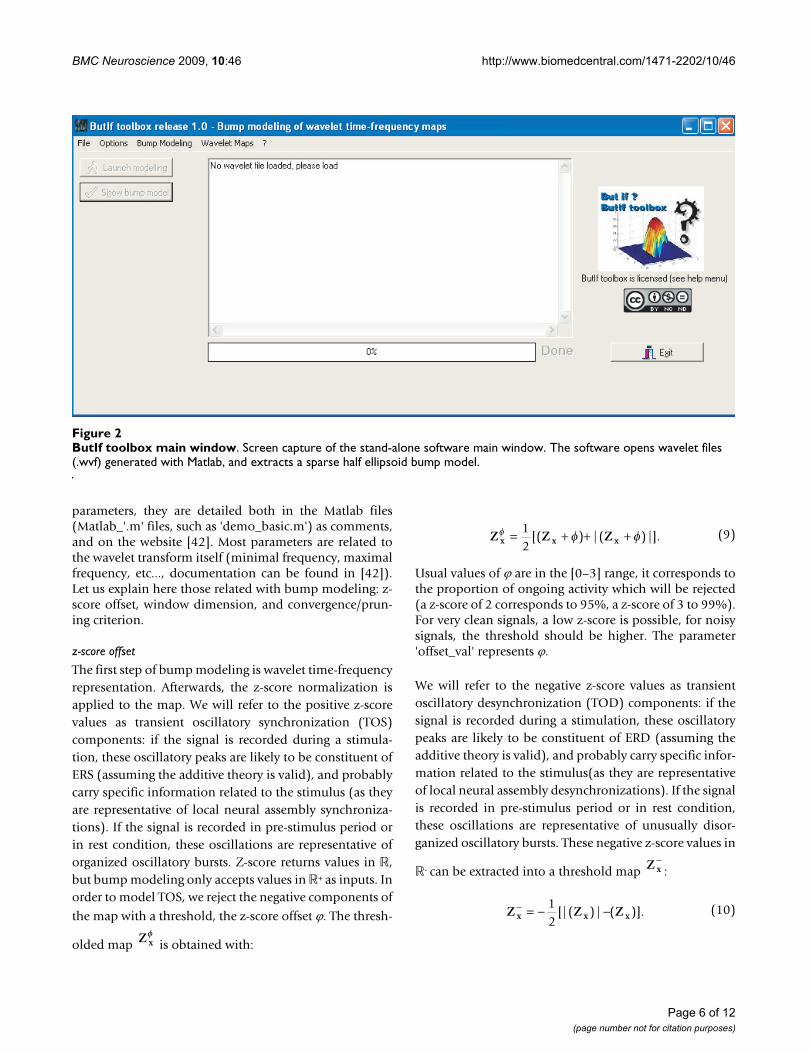
ButIf ToolboxThe toolbox is separated in two parts: One is a stand-alonesoftware (Fig. 2) developed using Borland C++ Builder2006. This standalone software is used to model bumpsfrom wavelet maps. It needs a Windows XP environmentto run. The second one is a set of Matlab m-files that per-form the wavelet transform and call the software. Theresulting bump model can be displayed using a Matlabfunction ('display_bumps.m'). The toolbox uses several

Ψ( , , , , , , )( , ) ( )

,A h w f t y xy f

h

x t

w= − + −

12

2

2

2(6)

ξλ

( , , , , , , ).

,A h w f t y xA

=<⎧

⎨⎩

0 if

else

ΨΨ

(7)

Ψ

E A h w f t y x s A h w f t y xy x

y

H

x

W

( , , , , , , ) || ( , ) ( , , , , , , ) ||,= −==

∑∑ ω τ ξ 2

11

..

(8)

Page 5 of 12(page number not for citation purposes)

BMC Neuroscience 2009, 10:46 http://www.biomedcentral.com/1471-2202/10/46

parameters, they are detailed both in the Matlab files(Matlab_'.m' files, such as 'demo_basic.m') as comments,and on the website [42]. Most parameters are related tothe wavelet transform itself (minimal frequency, maximalfrequency, etc..., documentation can be found in [42]).Let us explain here those related with bump modeling: z-score offset, window dimension, and convergence/prun-ing criterion.

z-score offset

The first step of bump modeling is wavelet time-frequencyrepresentation. Afterwards, the z-score normalization isapplied to the map. We will refer to the positive z-scorevalues as transient oscillatory synchronization (TOS)components: if the signal is recorded during a stimula-tion, these oscillatory peaks are likely to be constituent ofERS (assuming the additive theory is valid), and probablycarry specific information related to the stimulus (as theyare representative of local neural assembly synchroniza-tions). If the signal is recorded in pre-stimulus period orin rest condition, these oscillations are representative oforganized oscillatory bursts. Z-score returns values in �,but bump modeling only accepts values in �+ as inputs. Inorder to model TOS, we reject the negative components of

the map with a threshold, the z-score offset ϕ. The thresh-

olded map is obtained with:

Usual values of ϕ are in the [0–3] range, it corresponds tothe proportion of ongoing activity which will be rejected(a z-score of 2 corresponds to 95%, a z-score of 3 to 99%).For very clean signals, a low z-score is possible, for noisysignals, the threshold should be higher. The parameter'offset_val' represents ϕ.

We will refer to the negative z-score values as transientoscillatory desynchronization (TOD) components: if thesignal is recorded during a stimulation, these oscillatorypeaks are likely to be constituent of ERD (assuming theadditive theory is valid), and probably carry specific infor-mation related to the stimulus(as they are representativeof local neural assembly desynchronizations). If the signalis recorded in pre-stimulus period or in rest condition,these oscillations are representative of unusually disor-ganized oscillatory bursts. These negative z-score values in

�- can be extracted into a threshold map :

Z xφ

Z Z Zx x xφ φ φ= + + +1

2[( ) |( ) |]. (9)

Z x−

Z Z Zx x x− = − −1

2[|( ) | ( )]. (10)

ButIf toolbox main windowFigure 2ButIf toolbox main window. Screen capture of the stand-alone software main window. The software opens wavelet files (.wvf) generated with Matlab, and extracts a sparse half ellipsoid bump model.

Page 6 of 12(page number not for citation purposes)

BMC Neuroscience 2009, 10:46 http://www.biomedcentral.com/1471-2202/10/46

In order to model , the parameter 'offset_val' must begiven the value -1 in the model header.

Window DimensionWavelets have a specific time-frequency resolutiondepending on their central frequency [16,19]. This resolu-tion corresponds to their precision in time and frequency.Consequently, the representation of a high frequencytransient activity will be narrow in time and spread in fre-quency – conversely for low frequency transient activities.This is taken into account when establishing the adapta-tion windows. The dimension H × W (height and width)

of the windows ω depends on the time-frequency resolu-tion at the window's central frequency: the dimension Wis determined to have a duration of a fixed number of timeperiods, and the dimension H is determined as the ratioof W to the time-frequency resolution (see above, and[22]). This dimension should always be determined to fitthe average size of transient synchrony events, but is adap-tive with frequency (it does not usually need to bechanged for analyzing low or high frequency signals –because it is expressed in cycles). The parameter'header.cote' in the toolbox represents this fixed number,i.e. the number of oscillation one wishes to model. It wasobserved that TOS last around three to four cycles (oscil-

Z x−

Effect of the z-score offsetFigure 3

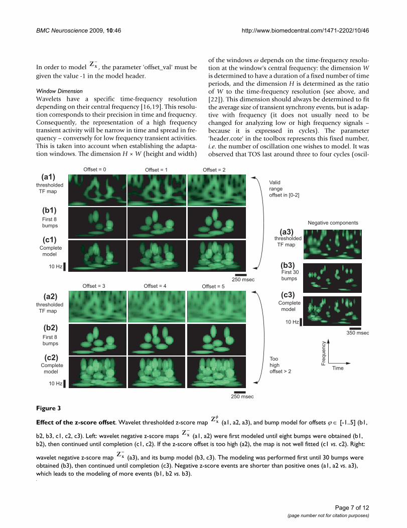
Effect of the z-score offset. Wavelet thresholded z-score map (a1, a2, a3), and bump model for offsets ϕ ∈ [-1..5] (b1,

b2, b3, c1, c2, c3). Left: wavelet negative z-score maps (a1, a2) were first modeled until eight bumps were obtained (b1, b2), then continued until completion (c1, c2). If the z-score offset is too high (a2), the map is not well fitted (c1 vs. c2). Right:

wavelet negative z-score map (a3), and its bump model (b3, c3). The modeling was performed first until 30 bumps were obtained (b3), then continued until completion (c3). Negative z-score events are shorter than positive ones (a1, a2 vs. a3), which leads to the modeling of more events (b1, b2 vs. b3).

Offset = 0 Offset = 1 Offset = 2

Offset = 3 Offset = 4 Offset = 5

thresholded TF map

First 8bumps

Complete model

thresholded TF map

First 8bumps

Complete model

Validrangeoffset in [0-2]

Toohighoffset > 2 Time

Freq

uenc

y

250 msec

10 Hz

250 msec

10 Hz

(a1)

(b1)

(c1)

(a2)

(b2)

(c2)

Negative components

thresholded TF map

First 30bumps

Complete model

(a3)

(b3)

(c3)

350 msec

10 Hz

Z xφ

Z x−

Z x−

Page 7 of 12(page number not for citation purposes)

BMC Neuroscience 2009, 10:46 http://www.biomedcentral.com/1471-2202/10/46

late three to four times then disappear) [22,36]. Negativeevents (TOD) are shorter in duration, lasting approxi-mately two time periods. The parameter 'header.cote'should usually be four to model TOS events; and two tomodel TOD events (as an illustration, see Fig. 3). How-ever, one can change these parameters if he wishes tostudy its relevance. In this case, take into considerationthat windows encompassing too many cycles wouldattempt to model several events with one bump; whereasa too short window would split the map in many unnces-sary atoms.

Convergence and PruningWe first design a model with the largest number of bumps– within a reasonable computation time. To that effect,the fraction of the total intensity of the map modeled bya given bump is computed:

This value is compared with a threshold Ft: when threeconsecutive bumps have F <Ft, modeling stops. Theparameter 'header.limit' (usually = 0.2) represents thisthreshold.

A tradeoff must be performed between accuracy and rele-vance (also termed 'bias-variance dilemma'): if thenumber of bumps in the model is too low, the latter willnot be accurate; if it is too large, irrelevant non-organizedinformation from the background EEG will be modeled.When modeling is finished using the above terminationcriterion, we use a pruning strategy. The Matlab program'prune_model.m' can be used to perform this pruning.Pruning can be performed with four options: pruning toremove only abnormal bumps (bumps with abnormallysmall amplitude, width or height, i.e. below 5.10-2); prun-ing to remove bumps with a threshold Ft2 ≥ Ft; pruning toremove all bumps after the N first modeled (modelingorder); or pruning to remove all bumps after the N first intime order. Users can combine these options, in order toobtain a clean and accurate representation.

ResultsHere we will demonstrate how this toolbox works using atoy signal, and illustrate the use of the three main param-eters (z-score offset, window dimension, and conver-gence/pruning). All files (signal, Matlab demonstration'.m' files, application) can be downloaded on the bumptoolbox project website. The toy signal('sig_example.mat', see Fig. 1) is an EEG signal taken fromone channel recorded in rest eyes closed condition(Biosemi system, 2048 Hz sampling rate, 2 sec). This dem-onstration can be reproduced by launching demo_zscore

under Matlab 7.0 (with the wavelet toolbox). Note thatdue to border effects of the wavelet transform, 500 msecare automatically rejected on both sides of the waveletmap by the toolbox prior to bump modeling – hence onlyone second was analyzed in the following examples.

z-score offsetWe vary the parameter 'offset_val' in the [0–5] range toshow its effect on modeling (offset_val > 3 is usually notworth try, it is only shown for demonstrative purpose).The resulting models (Fig. 3, left, a1-2, b1-2, c1-2) are inthe folder 'result demo_zscore). Obviously, a too permis-sive z-score offset (here offset_val > 2) will introducestrong bias in the model.

Using the parameter offset_val = -1, the negative compo-

nents can be modeled (Fig. 3, right, a3, b3, c3). Asillustrated on the figure, the negative events are even moretransient, and needs usually more bumps to be properlyrepresented.

Window Dimension

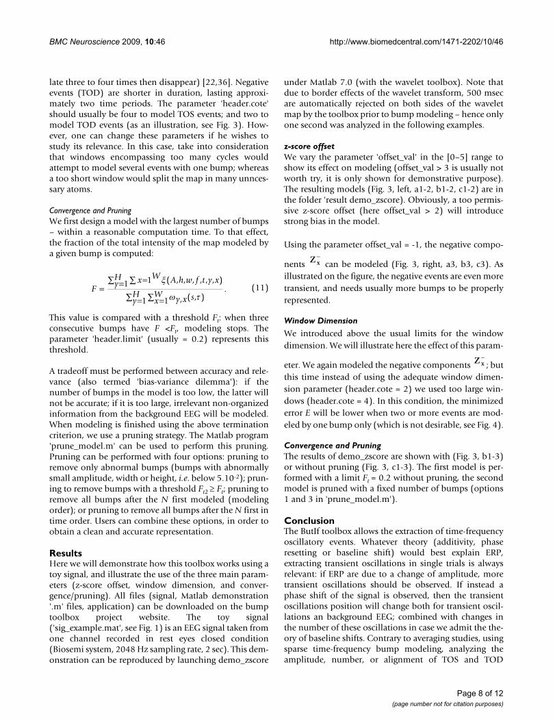
We introduced above the usual limits for the windowdimension. We will illustrate here the effect of this param-

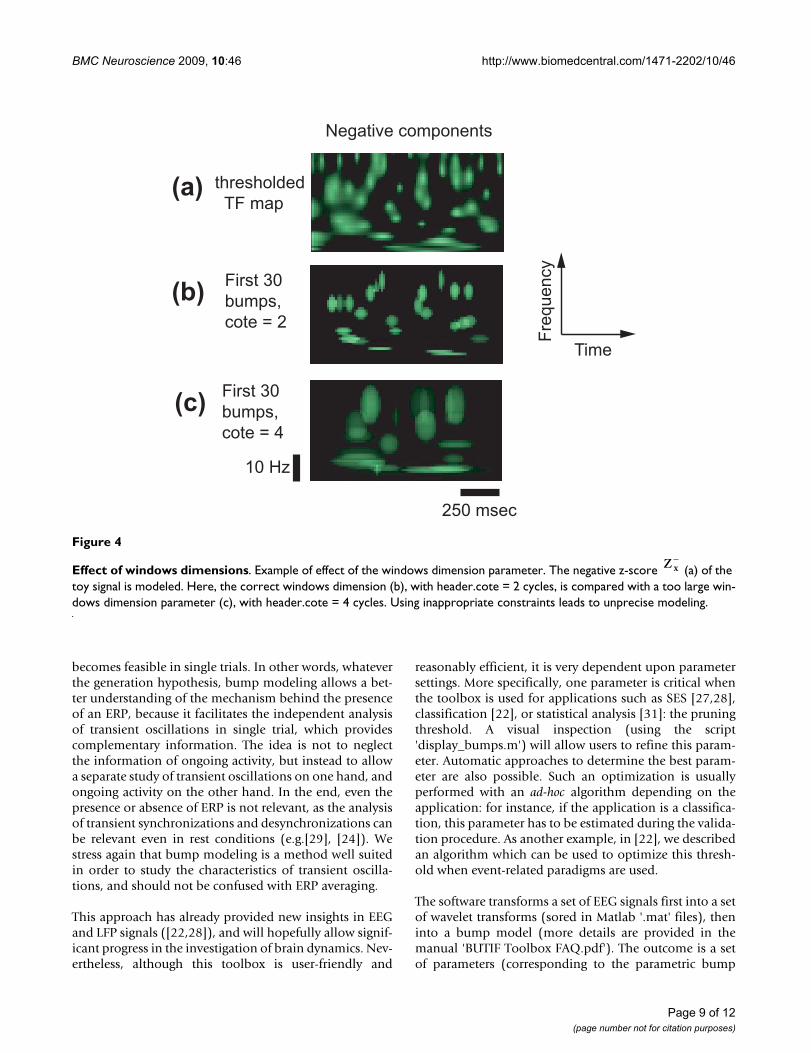
eter. We again modeled the negative components ; butthis time instead of using the adequate window dimen-sion parameter (header.cote = 2) we used too large win-dows (header.cote = 4). In this condition, the minimizederror E will be lower when two or more events are mod-eled by one bump only (which is not desirable, see Fig. 4).

Convergence and PruningThe results of demo_zscore are shown with (Fig. 3, b1-3)or without pruning (Fig. 3, c1-3). The first model is per-formed with a limit Ft = 0.2 without pruning, the secondmodel is pruned with a fixed number of bumps (options1 and 3 in 'prune_model.m').

ConclusionThe ButIf toolbox allows the extraction of time-frequencyoscillatory events. Whatever theory (additivity, phaseresetting or baseline shift) would best explain ERP,extracting transient oscillations in single trials is alwaysrelevant: if ERP are due to a change of amplitude, moretransient oscillations should be observed. If instead aphase shift of the signal is observed, then the transientoscillations position will change both for transient oscil-lations an background EEG; combined with changes inthe number of these oscillations in case we admit the the-ory of baseline shifts. Contrary to averaging studies, usingsparse time-frequency bump modeling, analyzing theamplitude, number, or alignment of TOS and TOD

Fx W A h w f t y xy

H

y x sxW

yH

==∑=∑

=∑=∑

11

11

ξ

ω τ

( , , , , , , )

, ( , ). (11)

Z x−

Z x−

Page 8 of 12(page number not for citation purposes)

BMC Neuroscience 2009, 10:46 http://www.biomedcentral.com/1471-2202/10/46

becomes feasible in single trials. In other words, whateverthe generation hypothesis, bump modeling allows a bet-ter understanding of the mechanism behind the presenceof an ERP, because it facilitates the independent analysisof transient oscillations in single trial, which providescomplementary information. The idea is not to neglectthe information of ongoing activity, but instead to allowa separate study of transient oscillations on one hand, andongoing activity on the other hand. In the end, even thepresence or absence of ERP is not relevant, as the analysisof transient synchronizations and desynchronizations canbe relevant even in rest conditions (e.g.[29], [24]). Westress again that bump modeling is a method well suitedin order to study the characteristics of transient oscilla-tions, and should not be confused with ERP averaging.

This approach has already provided new insights in EEGand LFP signals ([22,28]), and will hopefully allow signif-icant progress in the investigation of brain dynamics. Nev-ertheless, although this toolbox is user-friendly and

reasonably efficient, it is very dependent upon parametersettings. More specifically, one parameter is critical whenthe toolbox is used for applications such as SES [27,28],classification [22], or statistical analysis [31]: the pruningthreshold. A visual inspection (using the script'display_bumps.m') will allow users to refine this param-eter. Automatic approaches to determine the best param-eter are also possible. Such an optimization is usuallyperformed with an ad-hoc algorithm depending on theapplication: for instance, if the application is a classifica-tion, this parameter has to be estimated during the valida-tion procedure. As another example, in [22], we describedan algorithm which can be used to optimize this thresh-old when event-related paradigms are used.

The software transforms a set of EEG signals first into a setof wavelet transforms (sored in Matlab '.mat' files), theninto a bump model (more details are provided in themanual 'BUTIF Toolbox FAQ.pdf'). The outcome is a setof parameters (corresponding to the parametric bump

Effect of windows dimensionsFigure 4

Effect of windows dimensions. Example of effect of the windows dimension parameter. The negative z-score (a) of the toy signal is modeled. Here, the correct windows dimension (b), with header.cote = 2 cycles, is compared with a too large win-dows dimension parameter (c), with header.cote = 4 cycles. Using inappropriate constraints leads to unprecise modeling.

Negative components

thresholded TF map

First 30bumps,cote = 2

First 30 bumps,cote = 4

Time

Freq

uenc

y

250 msec

10 Hz

(a)

(b)

(c)

Z x−

Page 9 of 12(page number not for citation purposes)

BMC Neuroscience 2009, 10:46 http://www.biomedcentral.com/1471-2202/10/46

functions) stored in structured variable inside a Matlab'.mat' file. This variable can be visualized (displaying abump spectrogram, using the script 'display_bumps.m')or used for statistics. This provides a better understandingof the structure of EEG oscillations (TOS and TOD).Despite this toolbox provides many tools, some mainte-nance work will remain necessary in the future to improveand upgrade it. For instance, the choice of atom functionsaffects the modeling. We originally chose half ellipsoid fortheir sparsity (only five parameters); but despite a dissym-metric 2D curve would have more parameters, it mightbetter represent the dissymetry of wavelet representations(larger for lower frequencies). Until now we obtainedgood results with half ellipsoids, but this does not meanthat we might not find a better solution. Using othercurves is on the list of our future experimentations anddevelopments for the toolbox. Additionally, the pruningcriterion, as explained above, is critical. It would certainlybenefit from further investigations. New developments,however, will not be possible without interactions withusers (we invite questions, suggestions and comments;please see the website and its discussion forum for moredetails). Hence, the current version only lays the founda-tion stone of a long-term project.

Availability and requirementsProject name: ButIf toolbox

Project home page: http://www.bsp.brain.riken.jp/bumptoolbox/toolbox_home.html[42]

Operating system(s): Windows XP

Programming language: Matlab/C++ Builder 2006

Other requirements: Matlab 6.0 or 7.0 with wavelet tool-box is necessary to run this package (the wavelet toolboxcould also be replaced by a freeware wavelet toolbox, suchas the Uvi_Wave toolbox of Universidad de Vigo in Spain,which contains the complex Morlet wavelet).

License: Creative Commons License (CC-by-nc-nd) –Anyone can use this software for academic applicationsproviding they properly reference our work when publish-ing research results obtained with this toolbox (citing thepresent paper, and [22]).

Any restrictions to use by non-academics: the software isrestricted to non commercial applications.

Authors' contributionsFBV developed the concept of time-frequency bump mod-eling during his Ph.D., created the software, wrote the firstdraft of the paper, and created the first version of the web-site. JS-C helped in debugging of the final version of the

software, and for the preparation of the website (espe-cially the FAQ section). Reviewed the draft of the paper.JD helped in the theoretical development of bump mode-ling. Reviewed the draft of the paper. MM helped in thedesign of the website, was involved in the preparation ofall illustrations. AC helped in the theoretical develop-ments of bump modeling. Reviewed the draft of thepaper. All authors read and approved the final manu-script.

AppendixAppendix A: Improved Adaptation

In the previous implementation of bump modeling [22],we optimized all the bump function parameters (A, h, w,f, and t) simultaneously (first using iterations of first ordergradient descent, followed by iterations of the BFGS [40]algorithm). An improved adaptation can be obtained byoptimizing the parameters stepwise, with a prioritydepending on the order of their derivatives. When com-paring of the parameters derivatives (dE/dA, dE/dh, dE/dw,

dE/df and dE/dt), we observe that the term -2 is com-mon to all these derivatives, multiplyed by a term in �+:they will all have the same sign [41]. The slope of theadaptation will then be dependant on the multiplicands

m applied to -2E : m = 1 for dE/dA; m is a positivevalue in [0 - A] in numerator divided by a variable of order3 for dE/dh and dE/dw; m is a positive value in [0 - A] innumerator divided by a variable of order 2 for dE/df anddE/dt.

This would probably be working correctly with properlynormalized parameters, however we are here adaptingparameters of different ranges: A ∈ [0 - 1], while h and f ∈[1 - H/2] and w and t ∈ [1 - W/2] with H and W usually>> 1. Therefore, the multiplicands corresponding to thethree above case will be of the order m ∈ O(1) in case (1),and m ∈ O(x-3) in case (2) and m ∈ O(x-2) in case (3).Practically speaking, it means that the parameters adapta-tion should be performed stepwise (first h and w, then fand t, and finally A). We improved the quality and speedof convergence by performing the following stepwise esti-mation of these parameters:

1. Update h and w until both their derivatives arebelow a threshold tΨ.

2. Update f and t until both their derivative are belowa threshold tpos. If at anytime dE/dh or dE/dw becomesabove tΨ, go back to 1.

3. Update only A, until its derivative is below a thresh-old tA. If at anytime dE/dh or dE/dw becomes above tΨ,

EΨ

Ψ

Page 10 of 12(page number not for citation purposes)

BMC Neuroscience 2009, 10:46 http://www.biomedcentral.com/1471-2202/10/46

go back to 1. If at anytime dE/df or dE/dt becomesabove tpos, go back to 2.

The adaptation is still performed using the BFGS [40]algorithm.

Appendix B: Improved window matchingIn the previous version of bump modeling [22], the bestcandidate window Ω was selected as:

Because these windows are used to determine the initialcondition of the function adaptation, finding the bestsuitable window is primordial. The new optimizedmethod is more related to matching pursuit [20], in thatwe will match the window content w(f, t) with a prototypebump function ξw(f, t) = ξ(Aw, hw, lw, fw, tw, y, x) with fw = hw= H/2, xw, and Aw the highest peak in the window:

For each window w(f, t), we compute the correspondingmatrix Ξw(f, t) of values of this prototype function. Thebest window is thus matched as:

Where: denotes the Frobenius inner product, and ||·||Findicates the Frobenius norm. This generalize the match-ing criterion of matching pursuit methods to 2D data,with the difference that for bump modeling, high z-scorehas priority on best fit. Therefore, contrary to matchingpursuit, the product is not normalized by the norm of w.

Additional material

AcknowledgementsJordi Solé-Casals was supported by the Departament d'Universitats, Recerca i Societat de la Informació de la Generalitat de Catalunya, and by the Spanish grant TEC2007-61535/TCM. Monique Maurice is supported by the JSPS fellowship P-08811. Justin Dauwels is supported by the Henri-Ben-

edictus fellowship from the King Baudouin Foundation and the BAEF. F.B. Vialatte thanks Pr. R. Gervais (CNRS team NMO) and Pr. G. Dreyfus (ESPCI, Lab. d'Électronique) and collaborators (especially C. Martin, and R. Dubois) for their significant help in the early developments of the bump modeling methodology.

References1. Freeman W: A cinematographic hypothesis of cortical dynam-

ics in perception. International Journal of Psychophysiology 2006,60(2):149-161.

2. Le Van Quyen M: Disentangling the dynamic core: a researchprogram for a neurodynamics at the large-scale. BiologicalResearch 2003, 36:67-88.

3. Cosmelli D, Lachaux J, Thompson E: Neurodynamicalapproaches to consciousness. In The Cambridge Handbook of Con-sciousness Edited by: Zelazo P, Moscovitch M, Thompson E. NewYork: Cambridge University Press; 2007.

4. Varela F, Lachaux J, Rodriguez E, Martinerie J: The Brainweb:Phase Synchronization and Large-Scale Integration. NatureReviews Neuroscience 2001, 2(4):229-239.

5. Basar E: EEG-brain dynamics: Relation between EEG and brain evokedpotentials Amsterdam: Elsevier; 1980.

6. Basar E, Demilrap T, Schürmann M, Basar-Eroglu C, Ademoglu A:Oscillatory brain dynamics, wavelet analysis, ands cognition.Brain and Language 1999, 66:146-183.

7. Moratti S, Clementz B, Gao Y, Ortiz T, Keil A: Neural mechanismsof evoked oscillations: Stability and interaction with tran-sient events. Human Brain Mapping 2007, 28(12):1318-1333.

8. Klimesch W, Sauseng P, Hanslmayr S, Gruber W, Freunberger R:Event-related phase reorganization may explain evokedneural dynamics. Neuroscience and biobehavioral reviews 2007,31(7):1003-1016.

9. Risner M, Aura C, Black J, Gawne T: The Visual Evoked Potentialis independent of surface alpha rhythm phase. Neuroimage2009, 45(2):463-469.

10. Nikulin V, Linkenkaer-Hansen K, Nolte G, Lemm S, Müller K, Ilmo-niemi R, Curio G: A novel mechanism for evoked responses inthe human brain. European Journal of Neuroscience 2007,25(10):3146-3154.

11. Effern A, Lehnertz K, Schreiber T, David P, Elger C: Nonlineardenoising of transient signals with application to eventrelated potentials. Physica D 2000, 140:257-266.

12. Quiroga R, Sakowitz O, Basar E, Schürmann M: Wavelet transformin the analysis of the frequency composition of evokedpotentials. Brain Research Protocols 2001, 8:16-24.

13. Vialatte F, Solé-Casals J, Cichocki A: EEG windowed statisticalwavelet scoring for evaluation and discrimination of muscu-lar artifacts. Physiological Measurements 2008, 29(12):1435-1452.

14. R D, Maison-Blanche P, Quenet B, Dreyfus G: Automatic ECGwave extraction in long-term recordings using Gaussianmesa function models and nonlinear probability estimators.Comput Methods Programs Biomed 2007, 88(3):217-233.

15. Delprat N, Escudié B, Guillemain P, Kronland-Martinet R, P T, B T:Asymptotic wavelet and Gabor analysis: Extraction ofinstantaneous frequencies. IEEE Trans. Inform. Theory 1992,38:644-665.

16. Mallat S: A wavelet tour of signal processing 2nd edition. New York: Aca-demic Press; 1999.

17. Carroll J, Chang J: Analysis of individual differences in multidi-mensional scaling via an n-way generalization of 'Eckart-Young' decomposition. Psychometrika 1970, 35:283-319.

18. Acar E, Aykut-Bingol C, Bingol H, Bro R, Yener B: Multiway analysisof epilepsy tensors. Bioinformatics 2007, 23(13):i10-8.

19. Percival D, Walden A: Wavelet Methods for Time Series Analysis NewYork: Cambridge University Press; 2000.

20. Mallat S, Z Z: Matching Pursuits with Time-Frequency Dic-tionaries. IEEE Transactions on Signal Processing 1993, 12:3397-3415.

21. Gruber T, Müller M: Oscillatory brain activity dissociatesbetween associative stimulus content in a repetition primingtask in the human EEG. Cerebral Cortex 2005, 15:109-116.

22. Vialatte F, Martin C, Dubois R, Haddad J, Quenet B, Gervais R, G D:A Machine Learning Approach to the Analysis of Time-Fre-quency Maps, and Its Application to Neural Dynamics. NeuralNetworks 2007, 20:194-209.

Additional file 1All_In_One.zip. This file contains the ButIf toolbox 1.0, including the stand-alone software, Matlab package, demo files, sample data, and results of the demo. The 'documents' subfolder contains a manual (BUTIF Toolbox FAQ.pdf).Click here for file[http://www.biomedcentral.com/content/supplementary/1471-2202-10-46-S1.zip]

ΩΩ =⎡

⎣

⎢⎢

⎤

⎦

⎥⎥∑∑arg max ( , )

,f txy

f tw (12)

A f twf t

= max[ ( , )],

w (13)

ΩΩ =⎡

⎣⎢

⎤

⎦⎥arg max

( , ): ,|| ( , )||,f t

w f t f t

w f t F

ΞΞ

w(14)

Page 11 of 12(page number not for citation purposes)

BMC Neuroscience 2009, 10:46 http://www.biomedcentral.com/1471-2202/10/46

Publish with BioMed Central and every scientist can read your work free of charge

"BioMed Central will be the most significant development for disseminating the results of biomedical research in our lifetime."

Sir Paul Nurse, Cancer Research UK

Your research papers will be:

available free of charge to the entire biomedical community

peer reviewed and published immediately upon acceptance

cited in PubMed and archived on PubMed Central

yours — you keep the copyright

Submit your manuscript here:http://www.biomedcentral.com/info/publishing_adv.asp

BioMedcentral

23. Vialatte F, Martin C, Ravel N, Quenet B, Dreyfus G, Gervais R: Oscil-latory activity, behaviour and memory, new approaches forLFP signal analysis. Proceedings of the 35th annual general meetingof the European Brain and Behaviour Neuroscience Society (EBBS'03): 17–20 September Barcelona, Spain -Acta Neurobiologiae Experimentalis 2003,63:75.

24. Vialatte F, Cichocki A, Dreyfus G, Musha T, Shishkin SL, Gervais R:Early Detection of Alzheimer's Disease by Blind Source Sep-aration, Time Frequency Representation, and Bump Mode-ling of EEG Signals (invited presentation). LNCS 3696,Proceedings of the International Conference on Artificial Neural Networks2005 (ICANN'05): 11–15 September 2005, Warsaw, Poland2005:683-692.

25. Vialatte F, Cichocki A, Dreyfus G, Musha T, Rutkowski T, Gervais R:Blind source separation and sparse bump modelling of timefrequency representation of EEG signals: New tools for earlydetection of Alzheimer's disease. Proceedings of the IEEE Work-shop on Machine Learning for Signal Processing 2005 (MLSP'05): 28–30September 2005, Mystic CT, USA 2005:27-32.

26. Vialatte F, Cichocki A: Sparse Bump Sonification: a New Toolfor Multichannel EEG Diagnosis of Mental Disorders; Appli-cation to the Detection of the Early Stage of Alzheimer'sDisease. LNCS 4234, Proceedings of the 13th International Conferenceon Neural Information Processing (ICONIP'06): 3–6 October 2006, HongKong, China 2006:92-101.

27. Dauwels J, Vialatte F, Cichocki A: A novel measure for synchronyand its application to neural signals. Proceedings of the 32nd IEEEInternational Conference on Acoustics, Speech, and Signal Processing(ICASSP'07): 15–20 April 2007, Honolulu, USA 2007, IV:1165-1168.

28. Dauwels J, Vialatte F, Weber T, Cichocki A: Quantifying statisticalinterdependance by message passing on graphs: algorithmsand applications to neural signals – Part A. Neural Computation2009 in press.

29. Dauwels J, Vialatte F, Cichocki A: On Synchrony Measures for theDetection of Alzheimer's Disease based on EEG. LNCS 4984,Proceedings of the 14th International Conference on Neural InformationProcessing (ICONIP'07): 13–16 November 2007; Kita Kyushu, Japan2008:112-125.

30. Dauwels J, Vialatte F, Rutkowski T, Cichocki A: Measuring NeuralSynchrony by Message Passing. In Advances in Neural InformationProcessing Systems 20 Edited by: Platt J, Koller D, Singer Y, Roweis S.Cambridge, MA: MIT Press; 2008:361-368.

31. Vialatte F, Dauwels J, Rutkowski TM, Cichocki A: Oscillatory EventSynchrony During Steady State Visual Evoked Potentials. InAdvances in Cognitive Neurodynamics, Proceedings of the InternationalConference on Cognitive Neurodynamics 2007 Edited by: Wang R, Gu F,Shen E. Springer; 2008:439-442.

32. Buscema M, Rossini P, Babiloni C, Grossi E: The IFAST model, anovel parallel nonlinear EEG analysis technique, distin-guishes mild cognitive impairment and Alzheimer's diseasepatients with high degree of accuracy. Artificial Intelligence InMedicine 2007, 40:127-141.

33. Kronland-Martinet R, Morlet J, Grossmann A: Analysis of soundpatterns through wavelet transforms. International Journal onPattern Recognition and Artificial Intelligence 1988, 1(2):273-301.

34. Tallon-Baudry C, Bertrand O, Delpuech C, Pernier J: Stimulus spe-cificity of phase-locked and non-phase-locked 40 Hz visualresponses in human. Journal of Neuroscience 1996, 16:4240-4249.

35. Düzel E, Habib R, Schott B, Schoenfeld A, Lobaugh N, McIntosh AR,Scholz M, Heinze HJ: A multivariate, spatiotemporal analysis ofelectromagnetic time-frequency data of recognition mem-ory. Neuroimage 2003, 18:185-197.

36. Caplan J, Madsen J, Raghavachari S, Kahana M: Distinct patterns ofbrain oscillations underlie two basic parameters of humanmaze learning. J Neurophysiol 2001, 86:368-380.

37. Li X, Yao X, Fox J, Jefferys J: Interaction dynamics of neuronaloscillations analysed using wavelet transforms. Journal of Neu-roscience Methods 2007, 160:178-185.

38. Slobounov S, Hallett M, Cao C, Newell K: Modulation of corticalactivity as a result of voluntary postural sway direction: AnEEG study. Neuroscience Letters 2008, 442(3):309-313.

39. Vialatte F, Bakardjian H, Prasad R, Cichocki A: EEG paroxysmalgamma waves during Bhramari Pranayama: A yoga breath-ing technique. Consciousness and Cognition 2009 in press.

40. Press WH, Flannery BP, Teukolsky SA, T VW: Numerical recipes in C:The art of scientific computing New York: Cambridge University Press;2002.

41. Vialatte F, Dauwels J, Solé-Casals J, Maurice M, Cichocki A:Improved Sparse Bump Modeling for ElectrophysiologicalData. In Proceedings of the 15th International Conference on NeuralInformation Processing (ICONIP'08) – Part I, LNCS Volume 5506.Springer; 2009:224-231.

42. Vialatte F, Solé-Casals J, Dauwels J, Maurice M, Cichocki A: ButIftoolbox project. [http://www.bsp.brain.riken.jp/bumptoolbox/toolbox_home.html].

Page 12 of 12(page number not for citation purposes)