Detecting the time-dependent coherence between

non-stationary electrophysiological signals

–A combined statistical and time-frequency

approach

Yang Zhan† David Halliday† Xuguang Liu∗ Jianfeng Feng‡

†Department of Electronics, University of York

York, YO10 5DD, UK

∗ Charing Cross Hospital & Division of Neuroscience and Mental Health

Imperial College London, London, W6 8RF, UK

‡Department of Computer Science and Mathematics

University of Warwick, Coventry, CV4 7AL, UK

Research Article

December 6, 2005

1

Abstract

Various time-frequency methods have been used to study the time-varying

properties of non-stationary neurophysiological signals. In the present study, a

time-frequency coherence using continuous wavelet transform (CWT) together

with its confidence intervals are proposed to evaluate the correlation between

two non-stationary processes. A systematic comparison between approaches

using CWT and short-time Fourier transform (STFT) is carried out. Simu-

lated data are generated to test the performance of these methods when es-

timating time-frequency based coherence. Surprisingly and in contrast to the

common belief, the coherence estimation based upon CWT does not always

supersede STFT. We suggest that a combination of STFT and CWT would

be most suitable for analysing non-stationary neural data. In both frequency

and time domains, methods to test whether there are two coherent signals

presented in recorded data are presented. Our approach is then applied to

the electroencephalogram (EEG) and surface electromyogram (EMG) during

wrist movements in healthy subjects and the local field potential (LFP) and

surface EMG during resting tremor in patients with Parkinson’s disease. A soft-

ware package including all results presented in the current paper is available at

http://www.dcs.warwick.ac.uk/˜feng/software/COD.

Key words: Wavelet, Coherence, Confidence intervals, EEGs, EMGs, LFPs,

time discrimination, frequency discrimination

2

1 Introduction

Coherence analysis has been extensively applied in studying the neural activity within

nervous systems. Neurophysiological signals contain noise at all levels and are bound

to be treated as random signals or stochastic processes [17]. A single stationary

stochastic process is often characterised by its autocovariance function and its power

spectrum. Power spectrum is the Fourier transform of the autocovariance function

and provides us with the frequency description of the process. The frequency or

spectral contents of such signals display important information and have been used

to evaluate the physiological and functional state of the nervous systems. Fourier

analysis has been used extensively in studying the spectra of neurophysiological sig-

nals and in recent years interests have been focused on the study of synchronised

phenomena between two or more events, such as the synchronisation between brain

areas [2, 31] and correlation between electroencephalogram (EEG), electromyogram

(EMG) and magnetoencephalogram (MEG) [9, 21, 22, 7]. In general, the investigated

signals or data are assumed to be stationary and the estimates of the individual and

cross spectra are calculated to obtain the coherence estimate. Fourier analysis serves

as the fundamental coherence estimation method which yields the informative pe-

riodograms. Based on Fourier analysis and under Gaussian assumption, confidence

intervals of the estimated coherence can be estimated. The construction of the confi-

dence intervals is of vital importance since it allows the significant correlation to be

detected and statistically assessed at various frequency ranges.

A wide range of signals encountered in biomedical applications and nervous sys-

tems fall into the category of non-stationary signals whose statistical properties con-

stantly change with time. Such non-stationarity makes the Fourier analysis limited

when temporal information of how the signals’ frequency components evolve with

time is necessary to be looked at. Short-time Fourier transform (STFT), a method

which applies a short time window to the signal and performs a series of Fourier trans-

forms within the window as it slides across all the times, can overcome the problems

brought by Fourier analysis and form a time-frequency representation of the signals

3

of interest. Alternatively, the wavelet transform provides a useful approach in inves-

tigating non-stationary signals, which is usually regarded as an “optimal” solution to

the time and frequency resolutions. The wavelet analysis has previously been used

to study the EEG [29, 14, 30, 33] and EMG [26, 12]. Recently, transform methods

based on Fourier and wavelet analysis are compared in [3] in the application of neural

data. In order to evaluate the interactions within the nervous system, such as the

events of sensory stimulus and motor response, the relationship between simultane-

ously recorded neural and muscular data needs to be studied. To characterise and

detect the rhythms between two random processes, cross correlation and cross spec-

tral methods can be employed. Correlation detection based on wavelet transforms

has been used in wind engineering [8] and climatic and oceanic research [36]. In

recent years in connection with neurophysiological applications, cross spectrum and

coherence analysis have been used to analyse spike activity [25, 15].

The main contribution of our paper is the following. First, When it comes to

examine the relationship between two channels of signal recordings with multiple

trials, a time-frequency coherence based on continuous wavelet transform (CWT) is

proposed and the way of estimating its confidence intervals is described. Second, via

extensive simulations and in contrast to most results presented in the literature that

CWT has an obvious advantage over short-time Fourier transform (SFFT), we find

that SFFT performs better than CWT to detect low frequency signals, and CWT

works better for high frequency signals. Intuitively, this reflects the different intrinsic

properties of SFFT and CWT. At a low frequency (more stationary signals), CWT

which has a high nonlinearity than SFFT and is bound to perform worse. But at a

high frequency, SFFT becomes less sensitive to signals. Based upon our results, we

then suggest that a more reasonable approach to detect the coherence between two

signals would use both SFFT and CWT rather than use CWT alone. Third, purely

in terms of a time or frequency resolution, it is found that CWT usually outperforms

SFFT, in agreement with results in the literature. Methods on how to statistically

detect signals with different frequencies (frequency discrimination) or whether there

is a time gap (time discrimination) between signals are introduced.

4

Our approach is then successfully applied to experimental data: EEG-EMG ob-

tained from healthy subjects during a voluntary wrist movement task and LFP-EMG

obtained from Parkinson’s disease patients during involuntary resting tremor. In

summary, results presented here involve in how to statistically deal with three key

quantities in a time-frequency approach: magnitude, frequency and time, when multi-

trials physiological data are available. We expect that our approach could reveal

some fundamental facts when more massive data, for example, the LFPs recorded in

a multi-electrode array are available [11, 4, 34].

2 Methods

2.1 Coherence magnitude

2.1.1 Continuous Wavelet Transform (CWT)

−6 −4 −2 0 2 4 6−1

−0.5

0

0.5

1

t

(a) Morlet wavelet

0 1 20

0.5

1

1.5

2

f

(b) Energy spectrum

Figure 1: Morlet wavelet and its Fourier transform, f0 = 0.849. (a) Morlet wavelet.

The solid line is the real part and the dashed line is the imaginary part. The dotted

line is the envelope. (b) Fourier transform of Morlet wavelet, with the vertical dashed

line corresponding to the characteristic frequency f0.

The continuous wavelet transform (CWT) of x(t) is defined as

CWTx(a, b) =∫ ∞

−∞x(t)ψ∗a,b(t) dt (1)

5

where

ψa,b(t) =1√aψ

(t− b

a

)(2)

ψ(t) is called the mother wavelet where a is the dilation parameter, b is the location

parameter and ∗ denotes complex conjugate. The choice of the wavelet should satisfy

a number of selection criteria, such as the candidate functions having finite energy

and satisfying admissibility condition [1].

The CWT is usually presented as a time-frequency representation by converting

the scale parameter to the frequency. To fulfill this representation, a character fre-

quency f0 which is defined as the bandpass centre or central frequency of the wavelet

energy spectrum is chosen and by use of the relationship between the converted fre-

quency and arbitrary scale f = f0/a [1], the CWT can be expressed as

CWTx(τ, f) = CWTx(a, b)|a=

f0f

,b=τ=

√f

f0

∫ ∞

−∞x(t)ψ∗

(t− τ

f0

f

)dt (3)

One of the most commonly used wavelets in practice is the Morlet wavelet, defined

as

ψ(t) =1

π1/4(ej2πf0t − e−(2πf0)2/2) e−t2/2 (4)

where f0 is the central frequency of the wavelet. If the choice of f0 is appropriate the

second term in the bracket which is known as the correction term becomes negligible,

thus giving a simple Morlet wavelet [20]

ψ(t) =1

π1/4ej2πf0te−t2/2 (5)

This expression shows that Morlet wavelet is a complex sine wave within a Gaussian

envelope. The Fourier transform of the Morlet wavelet is

ψ(f) = π1/4√

2 e−12(2πf−2πf0)2 (6)

which has the form of a Gaussian function centred at f0 with f0 determining the wave

numbers within the envelope and in practice the value of 0.849 is often used. In Fig.

1 a Morlet wavelet with f0 = 0.849 and its Fourier transform are shown.

6

By employing the convolution theorem the wavelet transform can be expressed as

the product of the Fourier transforms of the signal and wavelet, x(f) and ψ(f)

CWTx(a, b) =√

a∫ ∞

−∞x(f)ψ∗(af)ej2πfb df (7)

This relationship provides a convenient way when implementing CWT on computer

since the Fourier transform of the wavelet function ψa,b(f) is already known in analytic

form. The computation only requires an FFT of the original signal and an inverse

FFT of the product of x(f) and ψ∗(af).

The square modulus of the wavelet transform is called the scalogram and is defined

as

SCALx(τ, f) = |CWTx(τ, f)|2 (8)

The scalogram is a time-varying spectral representation which describes the energy

distribution of the signal. The scalogram |CWTx(τ, f)|2 is often referred to as the

wavelet spectrum. This is sometimes multiplied by a constant factor to give a slightly

different expression [35, 1]. The wavelet spectrum gives a time-frequency representa-

tion, and it measures the contribution to the total energy coming from the vicinity

of a point at a specific time and frequency for a given mother wavelet [23].

Another commonly used time-frequency representation is short-time Fourier trans-

form (STFT) [28], defined as

STFTx(τ, f) =∫ ∞

−∞x(t)w(t− τ)e−j2πft dt =

∫ ∞

−∞x(t)w∗

t,f (t) dt (9)

where w∗t,f (t) = w(t − τ)e−j2πft. STFT analyses the signal x(t) through a short-

time window w(t): x(t)w(t − τ), and then a Fourier transform is performed on this

product using a set of basis functions. The square modulus of STFT is referred to as

the spectrogram

SPECx(τ, f) = |STFTx(τ, f)|2 (10)

In this report, both CWT and STFT are used for the coherence analysis and the

performance of the two is discussed in detail.

7

2.1.2 Time-Frequency Coherence

In order to study the relationship between two non-stationary processes definitions of

cross spectrum and coherence are desirable. Given two processes x(t) and y(t) with

their time-frequency representations X(τ, f) and Y (τ, f), the time-frequency cross

spectrum between them is defined as

Sxy(τ, f) = X(τ, f)Y ∗(τ, f) (11)

and the auto spectra are given by

Sx(τ, f) = |X(τ, f)|2 (12)

Sy(τ, f) = |Y (τ, f)|2 (13)

In the above equations, the X(τ, f) and Y (τ, f) can be based on either STFT or

wavelet transforms. The time-frequency based coherence, the square of the cross

spectrum normalised by the individual auto spectra, is defined by

R2xy(τ, f) =

|Sxy(τ, f)|2Sx(τ, f)Sy(τ, f)

(14)

The above definitions are straightforward and they follow a similar approach to the

Fourier analysis. In the Fourier analysis, the spectra and the coherence can be es-

timated by virtue of the periodogram method in which a number of segments are

averaged to obtain the estimation. However, in the case of time-frequency coherence

problems arise when using averaging because there are two dimensions of both time

and frequency. It is unclear along which direction the smoothing should be done [35].

As noted in [35], the coherence will have an identical value of one at all times and

frequencies without smoothing. In [8], a localised window T based on the time resolu-

tion is introduced to overcome this problem, however the choice of T is arbitrary and

can suffer from a lack of interpretation. In [13], the wavelet coherence is analysed and

the size of the smoothing window is chosen according to the oscillation cycles within

the window. However, this wavelet coherence is based on single-trial brain signals.

Here in the present report, a series of repeated trials are recorded and a consistent

relationship between two signals needs to be explored. In this connection a smoothing

8

scheme based on the repeated trials is proposed and the estimate of the coherence is

defined as

R2xy(τ, f) =

|Sxy(τ, f)|2Sx(τ, f)Sy(τ, f)

(15)

where

Sx(τ, f) =1

K

K∑

k=1

|Xk(τ, f)|2 (16)

Sy(τ, f) =1

K

K∑

k=1

|Yk(τ, f)|2 (17)

Sxy(τ, f) =1

K

K∑

k=1

Xk(τ, f)Y ∗k (τ, f) (18)

The above equations (15)-(18) outlines the procedure for estimating the time-

frequency coherence. The two channels of data contain a series of repeated trials

{x1(t) . . . xK(t)} and {y1(t) . . . yK(t)} that are recorded simultaneously. In each trial

xk(t) and yk(t), the time-frequency representations Xk(τ, f) and Yk(τ, f) are calcu-

lated and their squared magnitude |Xk(τ, f)|2 and |Yk(τ, f)|2 (spectrogram or scalo-

gram) as well as the cross spectrum Xk(τ, f)Y ∗k (τ, f) are calculated. After averaging

across these multiple trials, the estimates for auto spectra and cross spectrum are

obtained and they lead to the estimate of the time-frequency based coherence as ex-

pressed in (15). The average cross spectrum and its single-trial version consist of

complex values, and the amplitude and phase spectra can be defined as the absolute

value and angle respectively.

2.1.3 Confidence Intervals

In order to construct confidence intervals for the above time-frequency coherence some

basic assumptions about the investigated time series or stochastic processes must be

made. In Fourier analysis, the two time series are assumed to be stationary and a

theoretical distribution (e.g. Gaussian) is used to approximate the probability density

of the data.

However, because the time-frequency analysis contains temporal changes or time-

varying information, the description of the statistics is confined to a localised interval

9

[27]. The wavelet spectra has been compared to Fourier spectra in [23] and the vari-

ance of the wavelet spectrum was analysed in [24]. The wavelet spectrum based on

continuous wavelet transform was studied in [16]; where it was concluded that the

wavelet spectrum can represent the second-order statistical properties of random pro-

cesses for stationary and some non-stationary processes. It was shown that the local

wavelet spectrum follows the mean Fourier spectrum [35]. Based on this assumption,

the wavelet power spectrum should be χ2 distributed and confidence levels for the

cross-wavelet spectrum can be derived from the square root of the product of two χ2

distributions.

For the setting of confidence intervals for the time-frequency based coherence the

notion of generalised coherence is used here [6].

Let X = {Xk(τ, f)}Kk=1 and Y = {Yk(τ, f)}K

k=1 denote the complex time-frequency

representation of a sequence of repeated trials. Then the estimate of the coherence

in (15) can be denoted by

R2xy(τ, f) =

|〈X,Y〉|2‖X‖2 · ‖Y‖2

=

∣∣∣∣∣K∑

k=1Xk(τ, f)Y ∗

k (τ, f)

∣∣∣∣∣2

K∑k=1

|Xk(τ, f)|2 · K∑k=1

|Yk(τ, f)|2(19)

where 〈X,Y〉 is the inner product of X and Y, defined by

〈X,Y〉 =K∑

k=1

Xk(τ, f)Y ∗k (τ, f) (20)

‖X‖2 = 〈X,X〉 and ‖Y‖2 = 〈Y,Y〉 are the squared magnitudes of X and Y. The

time-frequency based coherence takes the values between 0 and 1 and in particular,

Rxy(τ, f) = 0 if X and Y are orthogonal, if X = aY for any non-zero complex number

a then Rxy(τ, f) = 1.

If the two processes are independent the coherence is particularly useful because no

common signal component is present. Under the hypothesis that the two processes

are independent Gaussian noise it allows thresholds corresponding to a particular

probability of false alarm to be set directly. The distribution of the coherence estimate

10

[6] is given by

Pr(R2 ≤ r) = 1− (1− r)K−1 , 0 ≤ r ≤ 1 (21)

where P (·) denotes the probability, and r is the detection threshold. For a confident

interval of probability 0.95, 1 − (1 − r)K−1 = 0.95, and the detection threshold is

r95% = 1 − 0.051/(K−1). This says that the estimate which is less than this value

should be regarded as insignificant.

The above construction of the confidence interval is based on the assumption that

the two processes have independent Gaussian distribution. However, as pointed out in

[5], the distribution of the coherence estimate does not depend on the statistics of one

of the two processes provided that the other process is Gaussian and the two processes

are independent. This property shows that the coherence estimate is invariant with

respect to the second channel statistics as long as one of the two independent processes

is Gaussian. This assumption can be further weakened by a geometric argument that

the process has spherically symmetric distribution (see Appendix A) instead of the

stronger Gaussian assumption [5, 32].

2.2 Discrimination in frequency domain

The time-frequency coherence analysis gives out a result in both the time and fre-

quency domain. Usually the result is illustrated through a graphic plot in the di-

mensions of time and frequency, thus a direct visual examination can reflect the

correlated components in the joint time-frequency plane. However, as for the non-

stationary signals, whichever approach either CWT or STFT is used, it is necessary to

use statistical methods to assess the frequency discrimination of both methods. More

exactly, assume that we find the maximum values of the coherence at two frequencies

f1 and f2, f2 6= f1, we want to statistically test whether f1 6= f2 or not.

The test for the frequency discrimination is important since it tells us the ability

of the coherence estimator to separately discriminate two correlated components that

are close in frequency. From this point, we can fix a frequency f1 where the two

processes are correlated at a given time interval, and then calculate the maximum

11

coherence value R(f1) at this frequency f1. For a nearby frequency f2 we can compute

its maximum coherence value R(f2). To test the frequency discrimination at these two

adjacent frequencies, we can generate enough testing data sets and derive the density

functions of R(f1) and R(f2): g1(f) and g2(f). To see if f2 can be discriminated from

f1, we can choose an observation value F = f0 where g1(f0) = g2(f0) and use the

following error probability as the discrimination criterion

Pr(F ≥ f0 | g1) = α (22)

If a 5% error probability is selected, i.e. when α < 0.05 we can say that the nearby

frequency f2 can be discriminated from f1.

How to tell one signal from another when noise is presented is a fundamental issue

in statistics. In classical statistics, two signals are separable as soon as noise vanishes.

Here, however, we are dealing with a totally different situation. From the uncertainty

principle, we know that even without noise, we have difficulty to distinguish between

two signals in time or frequency domain.

2.3 Discrimination in time domain

In this section, we aim to elaborate on the issue of time discrimination for the time-

frequency coherence using both STFT and CWT. Unlike the frequency discrimination

in which we can fix one frequency and see how close the nearby frequency can approach

the first fixed one until the second frequency cannot be identified, the coherence in the

time dimension is usually reflected as correlation during a time interval. It is difficult

to fix one interval and test the other nearby one since they can be chosen randomly

with each spanning different widths. Conversely, for a given frequency we can choose

two processes correlated across the entire time range but with a small period of the

same time interval in each process having no correlation at all. The width of this

gap period in the coherence analysis indicates the time discrimination ability and the

narrower the gap is, the better time discrimination result we will have.

Since the two processes have no correlation only in the gap interval, the coherence

12

estimate at the chosen frequency will have a significant dip around the chosen gap

but remain high amplitudes on the both sides of the dip. When the gap disappears

the coherence will jump back to the high amplitude around the original dip and hold

this amplitude for the entire time. Hence, one can calculate the distance between the

minimum coherence value at the dip and the neighbouring values where the coherence

jumps to the maxima. When the size of the gaps are reduced, we can see how narrow

the gap can reach until the coherence estimate can not distinguish the minimum and

maximum value of the dip, i.e. those two values are too near to be discriminated.

When the maximum and minimum values from the sample data are available, one

can obtain the distributions of the two quantities. A statistical test can be used to

test if these two maximum and minimum values are equal, e.g. t-test.

3 Results

3.1 Simulated data

In order to test the performance of the time-frequency coherence defined above, ar-

tificial data was generated to simulate the processes containing repeated trials. The

two test time series are Gaussian white noise with sine waves embedded in each trial

of the two processes. The signal-to-noise ratio (SNR), which is the logarithm ratio

of the power of the sine wave and the power of the white noise, is set to be −10 dB,

−15 dB and −20 dB. The Gaussian white noise used here have unit power and the

amplitudes of sine wave in each trial are adjusted according to the value of SNR to

satisfy the SNR settings.

Figure 2 shows a typical three-dimensional plot of the time-frequency coherence

defined above and in this example only the coherence using CWT is given as illustrat-

ing the general idea of the coherence distribution in both time and frequency. The

SNR was chosen as −10 dB and 20 trials were used. The plane in the figure shows

the 95% confidence interval calculated based on (21). The sine waves with 25 Hz were

embedded into the white noises from 500 ms to 600 ms in each trial of both white

13

noises. A significant peak can be seen in the estimates of both the STFT and wavelet

coherence between 500 ms and 600 ms and around 25 Hz in the time-frequency plane.

This illustrates clear correlation over specific ranges of time and frequency.

Figure 2: Time-frequency coherence using CWT of two Gaussian white noises of 1000

ms with two sine waves of 25 Hz which were embedded from 500 ms to 600 ms in each

channel. The SNR was set to be −10 dB and 20 trials were generated with sampling

rate 1 kHz. Morlet wavelet was used with f0 = 0.849.

In Fig. 3, time-frequency coherence estimates are shown using two different time-

frequency representations STFT and CWT under two SNR settings, −15 dB and −20

dB. The numbers of trials here were 50 and 200 for −15 dB and −20 dB, respectively.

For different SNRs, the number of trials was also chosen to be different in order to

detect the correlation under lower SNR settings. The results will improve if more trials

are used in the estimation. In general the two methods could successfully resolve the

correlation at both the three different time intervals in which three signal components

are embedded and the three different frequencies under low SNR settings. The window

length in the STFT was 300 ms, if a shorter window was used the results gave a good

time resolution but the frequency resolution became poor. This reflects the trade off

between time and frequency resolution inherent in the STFT method. The wavelet

14

coherence, using a complex Morlet wavelet, achieves to give a compromised result

between time and frequency resolution. The wavelet transform analyses the high

frequency parts with better time resolution and low frequency part with poorer time

resolution. Compared to the fixed time-frequency resolution for each frequency in

STFT, the wavelet analysis holds this demanding property. Both the STFT and

wavelet satisfy the uncertainty principle and are bounded by the Heisenberg box in

the time-frequency domain [1]. For the simulation result of the test data here which

contains three different frequency components 5 Hz, 25 Hz and 40 Hz, STFT gives a

better resolution than CWT at the low 5 Hz frequency, while CWT performs better for

the higher 25 and 40 Hz frequencies. When the two methods are applied to more test

data, it holds the result that STFT performs better than CWT at the low frequencies

but gives a poorer result at the higher frequencies (see Fig. 4). It is readily seen from

Fig. 4 that when the frequency is below 12 Hz, the coherence calculated based on

STFT is higher than that of CWT. In other words, the low frequency coherence is

more easily detected using STFT than CWT. This shows that a reasonable way to

analyse the coherence is to average out the pros and cons of the two. Our results are

then tested for a wide range of SNR settings (not shown here).

Fig. 4 also tells us another two interesting issues: time and frequency discrim-

ination for both methods. Bottom two right figures of Fig. 4 basically say that a

much better frequency resolution is achieved when the coherence frequency is high

(say > 10 Hz). For time resolution (top two right figures of Fig. 4), it is difficult to

draw a conclusion intuitively. In the next two subsections, we discuss and compare

the frequency discrimination and time discrimination of the two methods in details

based on our statistical test methods.

3.2 Test on frequency discrimination

In fact, a closer look at Fig. 4 bottom right reveals some interesting features for

CWT and STFT analysis. At a low frequency (≤ 10 Hz), for STFT the coherence

reaches its maxima between 0 and 1 Hz, despite the fact that the true coherence

should be at 1, 2, · · · , 10Hz. In other words, the frequency resolution is very low at a

15

0 100 200 300 400 500 600 700 800 900 1000−4

−2

0

2

4

Ch

an

ne

l 1

One trial of the test data −15dB, 50Trials

0 100 200 300 400 500 600 700 800 900 1000−4

−2

0

2

4

Time (ms)

Ch

an

ne

l 2

5Hz 25Hz 40Hz

Hz

STFT

0 200 400 600 8001000

10

20

30

40

50

ms

Hz

0 200 400 600 8001000

10

20

30

40

50

Wavelet

0 200 400 600 8001000

10

20

30

40

50

ms0 200 400 600 8001000

10

20

30

40

50

−15dB

−20dB

Figure 3: Time-frequency coherence using STFT and wavelet CWT under two dif-

ferent SNRs of −15 dB and −20 dB. Three sine wave components with different

frequencies were embedded into the Gaussian white noises in each trial at 200-300 ms

with 5 Hz, 400-500 ms with 25Hz and 600-700 ms with 40 Hz. Different trials were

generated for different SNRs with sampling rate 1 kHz, 50 trials at −15 dB and 200

trials at −20 dB. In the figure, the left column used STFT and the right column used

the CWT. From the top to the bottom, the SNR was set to be −10 dB and −15 dB,

respectively. In the STFT, the Gaussian data window of width 300 ms was used. The

CWT used Morlet wavelet with f0 = 0.849.

16

0 5 10 15 20 25 30 35 40 45 500

0.1

0.2

0.3

0.4

0.5

0.6

Frequency (Hz)

Cohere

nce

WaveletSTFT

0 10 20 30 40 50

100

200

300

Tim

e

Wavelet

0 10 20 30 40 50

1020304050

Frequency

Fre

qu

en

cy

0 10 20 30 40 50

100

200

300STFT

0 10 20 30 40 50

1020304050

Frequency

Figure 4: (Left): Use one white noise series, length 500 ms, with only a single period

of sine waves embedded, from 200 ms to 300 ms. The sine waves are selected to

have the frequencies from 1 Hz to 50 Hz and the coherence is calculated for each

frequency as it moves from 1 to 50 Hz in order to compare the two methods for all

these frequencies. The amplitude of the STFT coherence is adjusted to have the same

maximum height as CWT to allow for a uniformed scale for the comparison of the

two. A critical frequency at around 12 Hz is clearly shown. (Right): The data used is

the same as above: the test data consists of 500 ms white noise and a single period of

sine waves are embedded from 200 to 300 ms with the frequencies moving from 1 Hz

to 50 Hz at which frequency the coherence is calculated and the maximum value is

obtained for each frequency. It shows that at which time and frequency the coherence

of STFT and CWT reach its maximum value. Generally speaking, both methods can

pick up these correlations at the frequencies and time intervals where the sine waves

are added.

17

low frequency. This is also true for the case of CWT. How is the frequency resolution

at a high frequency?

0 10 20 30 40 500

0.05

0.1

0.15

0.2

0.25

0.3

0.35

20Hz →

← P=0.05

← 23Hz

← 25Hz

Frequency (Hz)

His

togra

m

Frequency discrimination for CWT

0 10 20 30 40 500

0.05

0.1

0.15

0.2

0.25

0.3

0.35

20Hz →

← P=0.05

← 25Hz

← 28Hz

Frequency (Hz)

His

togra

m

Frequency discrimination for STFT

Figure 5: 100 independent sets of test data are generated (SNR -10 dB, Trials 20)

for each histogram. The first frequency is chosen to be f1 = 20 Hz. A 5% error

probability was selected as the discrimination criterion, i.e. when the error is less

than this value it can be said that the nearby frequencies f2 can be discriminated

from f1. Form the figures, one can see that for STFT f2 = 28 Hz, for CWT f2 = 26

Hz.

To this end, we used our method for frequency discrimination and generated 100

independent sets of test data (SNR -10 dB, Trials 20). The first frequency was chosen

to be fixed at f1 = 20 Hz and the distribution of its maximum coherence value of the

100 sets is approximated by a normal distribution (see Fig. 5). A 5% error probability

was selected as the discrimination criterion, i.e. when the error is less than this value

it can be said that the nearby frequencies f2 is different from f1. For a given frequency

f2, 100 independent samples of the maximum coherence value were generated again

and is approximated by another normal distribution. From Fig. 5 one can see that

for STFT the critical frequency is around f2 = 28 Hz, but for CWT it is f2 = 25

Hz. Hence if we observe that one coherence arrives at its maximum value at 20 Hz,

and the other attains at 26 Hz for CWT analysis, we can assess there are two signals

18

with different frequencies, with a probability of 95%. For STFT analysis, we require

that the other signal should be with a frequency higher than 28 Hz so that we could

statistically discriminate between them.

As we mentioned, for the frequency result in Fig. 4 both STFT and CWT indicate

a very coarse frequency resolving ability under 10 Hz in the low frequency range. To

show the frequency discrimination in this range, we plot the discrimination results

for the frequencies from 1 Hz to 10 Hz in Fig. 6. Unlike the clear discrimination

result given at the frequency of 20 Hz, it is generally difficult to say if one frequency

can be discriminated from the others in the low frequency range < 10Hz for both

CWT and STFT. In the CWT result, the frequency distribution at 1 Hz is not shown

because the mean frequency for the 100 tests is around 20 Hz which is significantly

biased. However, if specifying a fixed frequency at 5 Hz we can still discriminate

the nearby frequencies from 8 Hz onwards. For the STFT result we can hardly find

any discriminated frequencies from each other since their distributions are all centred

around certain frequencies between 1 and 5 Hz. The frequency distributions at 3

Hz, 4 Hz and 5 Hz are not shown because the distribution for these three is a delta

function at 1 Hz for all 100 samplings.

3.3 Test on time discrimination

Using the test method for the time discrimination in section 2.3, again 100 samples are

generated for time gaps of 5, 10, 20 and 50 ms. The average results for both methods

are shown in Fig. 7 bottom two panels. It is seen that CWT has a narrower strip

in frequency domain than STFT, in agreement with what we claimed in the previous

subsection. However, from the average results, one might conclude that STFT has a

higher resolution in time than CWT. When the time gap is only 5 ms, we could see

there is a small dip in STFT coherence, but it is almost flat for CWT. When the time

gap is 50 ms, the coherence obtained from STFT approach is discontinuous, but not

for CWT.

To statistically confirm our conclusions, we then plot the coherence vs. time when

the frequency is fixed at 20 Hz in Fig. 7 upper panel left. The t-value is read out

19

−20 −15 −10 −5 0 5 10 15 20 25 300

0.1

0.2

0.3

0.4

0.5

← 5Hz

2Hz →

← 3Hz

← 4Hz

6Hz →

← 7Hz

← 8Hz

← 9Hz

← 10Hz

Frequency (Hz)

His

tog

ram

CWT discrimination in low frequency range

−20 −15 −10 −5 0 5 10 15 20 25 300

0.1

0.2

0.3

0.4

← 1Hz

← 2Hz

← 6Hz

← 7Hz← 8Hz

← 9Hz← 10Hz

Frequency (Hz)

His

tog

ram

STFT discrimination in low frequency range

Figure 6: Frequency discrimination in the low frequency range from 1 Hz to 10 Hz:

100 independent sets of test data are generated (SNR -10 dB, Trials 20) for each

histogram. 100 independent sets of test data are generated (SNR -10 dB, Trials 20)

for each histogram. Left, CWT method and frequency at 1 Hz is not shown; Right,

STFT method and frequencies at 3 Hz, 4 Hz and 5 Hz are not shown.

20

0 200 400 600 800 10000.3

0.350.4

0.450.5

0.550.6

0.650.7

0.750.8

0.85

TIme (ms)

Cohere

nce

0 10 20 30 40 500

10

20

30

40

50

Time gaps (ms)t valu

e

CWTSTFT

Time (ms)

Fre

qu

en

cy (

Hz)

0 200 400 600 800 1000

10

20

30

40

50

Time (ms)

Fre

qu

en

cy (

Hz)

0 200 400 600 800 1000

10

20

30

40

50

Time (ms)

Fre

qu

en

cy (

Hz)

0 200 400 600 800 1000

10

20

30

40

50

Time (ms)F

req

ue

ncy (

Hz)

0 200 400 600 800 1000

10

20

30

40

50

Time (ms)

Fre

qu

en

cy (

Hz)

gap 5 ms

0 200 400 600 800 1000

10

20

30

40

50

Time (ms)

Fre

qu

en

cy (

Hz)

0 200 400 600 800 1000

10

20

30

40

50

Time (ms)

Fre

qu

en

cy (

Hz)

0 200 400 600 800 1000

10

20

30

40

50

Time (ms)

Fre

qu

en

cy (

Hz)

0 200 400 600 800 10000

10

20

30

40

50

Figure 7: Top left, coherence averaged across 100 samples using CWT with a fixed

frequency at 20 Hz and the eight lines delving in the middle with different depths

from the top to the bottom correspond to the time gaps from 10 ms to 80 ms (see

figures at bottom and middle panels). Top right, calculated t-value as described in

the text. Middle panel, averaging coherence in frequency-time domain for STFT.

Bottom panel, averaging coherence in frequency-time domain for CWT. From the

left to the right, four columns correspond to the time gaps of 5, 10, 20 and 50 ms

21

from carrying out t-test for the maximum and minimum coherence values around the

time gaps. Surprisingly we found that the t-test gives us completely different results.

Fig. 7 upper panel right clearly indicates that again CWT is better than STFT: all

t-values obtained from CWT are higher than STFT, although the results tell us that

both methods have rather high time resolution. With a time gap of 5 ms, we are still

able to tell if there are two signals presented or not.

3.4 Data with unmatched sine waves

Time (ms)

Fre

quency (

Hz)

STFT Coherence

0 100 200 300 400 500

5

10

15

20

25

30

35

40

45

50

Time (ms)

Fre

quency (

Hz)

Wavelet Coherence

0 100 200 300 400 500

5

10

15

20

25

30

35

40

45

50

Figure 8: Coherence analysis with unmatched sine wave in each trial of the two

channels of test data. The data consists of 20 trials with SNR -10 dB and unmatched

sine waves are embedded into 200-300 ms interval of the 500 ms length in each trial.

The choice of the analysing window for STFT and wavelet for CWT is the same as

in the simulated data. Regions above the 95% confidence interval are shown. Left:

STFT method; Right: CWT method.

The above simulated data are generated using the sine waves which are symmet-

rically embedded into every single trial of each channel. In real applications, this

may not be the case because the harmonious components in each trial are unlikely

to be homogeneous although recordings come from repeated trials. In order to test

22

the influence of the inhomogeneity in each trial, unmatched sine waves are used in

each trial. In one channel 25% of the total sine waves in each trial are taken out

randomly while the other channel remain the same with no sine waves taken out. For

the results shown in Fig. 8, the sine waves have the frequency of 20 Hz with the SNR

setting -10 dB and trial number 20. The coherence from the both methods reaches

the correlation at 20 Hz between 200-300 ms in which the sine waves are embedded.

However, for the CWT coherence, there appears other less significant peaks at other

frequencies and time intervals. It suggests that inhomogeneity can create other co-

herence values which are not presented in the signals using the CWT method, though

this inhomogeneity is less prominent in the STFT method.

3.5 Application to Neural and Muscular Signals

3.5.1 Movement-related signals

As an illustration of the above time-frequency coherence, an example with application

to neural signals is given in this section. The data that contains simultaneously

recordings of EEG and EMG was collected during the voluntary movements of wrist

extension/flexion. The two pair of EEG electrodes were placed 2.5 cm lateral to

the vertex (Cz) with spacing 2.5 between each other while the EMG electrodes were

attached to the extensor forearm muscle [9]. The subjects repeatedly perform moving

and holding movements between the extension and flexion positions. Fig. 9 left

shows a period of EEG and EMG signals recorded from subjects’ performing such

wrist moving and extending movement. In this figure, 0-1.5 s is the is the moving

period when the wrist start moving towards extension position and 1.5-3.5 s is the

maintaining period when the wrist holds at the extension position. Before taking

the coherence analysis, both channels of data are preprocessed to have their mean

subtracted and trend removed, and for the EMG a full wave rectification is applied.

Wavelet coherence analysis of EEG and EMG signals during wrist moving and

extending periods is shown in Fig. 9. Forty repeated trials of moving and extending

movement were included. The subjects followed the auditory cues which were used

23

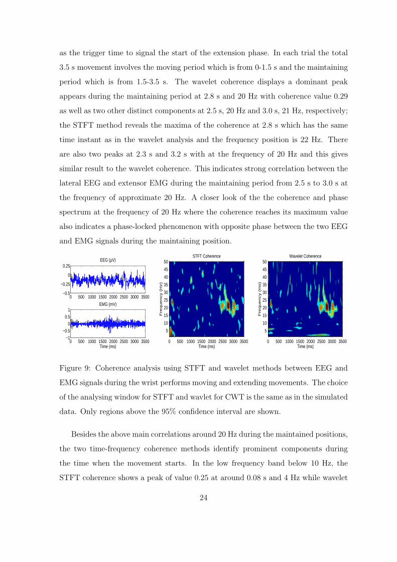
as the trigger time to signal the start of the extension phase. In each trial the total

3.5 s movement involves the moving period which is from 0-1.5 s and the maintaining

period which is from 1.5-3.5 s. The wavelet coherence displays a dominant peak

appears during the maintaining period at 2.8 s and 20 Hz with coherence value 0.29

as well as two other distinct components at 2.5 s, 20 Hz and 3.0 s, 21 Hz, respectively;

the STFT method reveals the maxima of the coherence at 2.8 s which has the same

time instant as in the wavelet analysis and the frequency position is 22 Hz. There

are also two peaks at 2.3 s and 3.2 s with at the frequency of 20 Hz and this gives

similar result to the wavelet coherence. This indicates strong correlation between the

lateral EEG and extensor EMG during the maintaining period from 2.5 s to 3.0 s at

the frequency of approximate 20 Hz. A closer look of the the coherence and phase

spectrum at the frequency of 20 Hz where the coherence reaches its maximum value

also indicates a phase-locked phenomenon with opposite phase between the two EEG

and EMG signals during the maintaining position.

0 500 1000 1500 2000 2500 3000 3500−0.5

−0.25

0

0.25EEG (µV)

0 500 1000 1500 2000 2500 3000 3500−1

−0.50

0.51

Time (ms)

EMG (mV)

Time (ms)

Fre

quency (

Hz)

STFT Coherence

0 500 1000 1500 2000 2500 3000 3500

5

10

15

20

25

30

35

40

45

50

Time (ms)

Fre

quency (

ms)

Wavelet Coherence

0 500 1000 1500 2000 2500 3000 3500

5

10

15

20

25

30

35

40

45

50

Figure 9: Coherence analysis using STFT and wavelet methods between EEG and

EMG signals during the wrist performs moving and extending movements. The choice

of the analysing window for STFT and wavlet for CWT is the same as in the simulated

data. Only regions above the 95% confidence interval are shown.

Besides the above main correlations around 20 Hz during the maintained positions,

the two time-frequency coherence methods identify prominent components during

the time when the movement starts. In the low frequency band below 10 Hz, the

STFT coherence shows a peak of value 0.25 at around 0.08 s and 4 Hz while wavelet

24

coherence shows a peak of value 0.19 at around 0.08 s and 0.6 Hz. This indicates the

correlation occurs at the movement onset and STFT gives a larger coherence value

than the CWT method in the low frequency range. Another correlation happens

during this moving period is at the frequency of around 23 Hz with the time 0.1 s,

and both the STFT and CWT methods yield the same level of coherence amplitude.

The remaining peak that appears at the low frequency under 5 Hz around 2.5 s in

the CWT method whereas is not presented in the STFT result may attribute to

the unmatched oscillatory patterns in each trial or any disturbance which causes

the difference across the trials during the recording. This reflects the inhomogeneity

brought by the unmatched signal components investigated in Section 3.4.

From Fig. 9, we can see that there three major coherence components. For CWT,

they are on the time of 2.5 s at 20 Hz, 2.8 s at 20 Hz and 3.0 s at 21 Hz. For STFT,

they are 2.3 s at 22 Hz, 2.8 s at 20 Hz, and 3.2 s at 20 Hz. The SNR, calculated

as the ratio of the power from 1-250 Hz and from 251-500 Hz, is < −10.2091 dB,

hence our results given in the section of simulated data can be directly applied here.

There are three broken and coherent signals in the coherence plot, suggesting that

significant coherence appears in different time periods but it is unclear whether they

are statistically independent in frequency.

3.5.2 Tremor-related signals

Deep brain stimulation is regarded as an effective approach for the clinical treatment

of Parkinson’s disease and it also provides the opportunity to study neuronal activity

recorded from the implanted electrode for chronic stimulations of subthalamic nucleus

(STN)[18, 19]. As another example of the application of the proposed time-frequency

coherence analysis, STN local field potentials (LFPs) and surface EMGs from the fore-

arm extensor muscle were simultaneously recorded from Parkinson’s disease patients

during resting tremor were analysed here.

Fig. 10 shows a period of typical LFP and the EMG signals during the intermittent

tremor as well as the time-frequency analysis of the two signals. The data has a

recording of 66 s with sampling frequency 500 Hz and it was partitioned into 33

25

segments with 2 s in each trial. At a first glance, we can see that both the STFT

and CWT coherence analyses indicate strong correlations in the low frequency range

under the 10 Hz. There are also additional clear features at other frequencies. The

CWT coherence reaches its maximum value of 0.22 at 20 Hz and 1.57 s, and around

this position STFT has a peak of value 0.13 at 19 Hz and 1.58 s. The maximum

value for STFT coherence is 0.21 at 12 Hz and 1.30 s, and around this position the

CWT coherence has a peak of 1.19 at 11 Hz and 1.29 s. The CWT coherence also

has a significant peak at 29 Hz and 0.59 s with the value of 0.21 while around this

position the STFT shows a relatively small peak at 22 Hz and 0.67 s with the value of

0.14. This says a higher CWT coherence value at higher frequencies according to our

previous analysis of the two. Other corresponding significant coherence for the two

methods of CWT vs. STFT in 10-15 Hz frequency range is at the following positions:

0.29 s 14 Hz (Coherence: 0.15) vs. 0.26 s 15 Hz (Coherence: 0.14), 1.07 s 14 Hz

(Coherence: 0.19) vs. 1.08 s 15 Hz (Coherence: 0.14).

0 0.4 0.8 1.2 1.6 2.0−50

−25

0

25

50LFP (mV)

0 0.4 0.8 1.2 1.6 2.0−2

−1

0

1

TIme (s)

EMG (mV)

Time (s)

Fre

quency (

Hz)

STFT Coherence

0 0.4 0.8 1.2 1.6 2.0

5

10

15

20

25

30

35

40

45

50

Time (s)

Fre

quency (

Hz)

Wavelet Coherence

0 0.4 0.8 1.2 1.6 2.0

5

10

15

20

25

30

35

40

45

50

Figure 10: STFT and wavelet coherence of STN LFP and EMG signals for the Parkin-

son’s disease patients and only regions above the 95% confidence interval are shown.

The choice of the analysing window for STFT and wavlet for CWT is the same as in

the simulated data.

If we look at the low frequency band under 10 Hz, there are three major significant

peaks. For CWT they are at 0.01 s 5 Hz (Coherence: 0.13), 0.79 s 3 Hz (Coherence:

0.12) and 1.45 s 5 Hz (Coherence: 0.17); for STFT they are at 0.12 s 4 Hz (Coherence:

0.20), 0.85 s 3 Hz (Coherence: 0.20) and 1.47 s 7 Hz (Coherence: 0.17). At these low

26

frequencies, the coherence values estimated from STFT seem to be generally higher

than CWT, confirming that at low frequency range of < 10Hz STFT yields higher

coherence values than CWT. However, for both CWT and STFT we can clearly see

that strong correlations occur during the whole time course of 2.0 s at low frequency

band of 3-7 Hz. Our results here are in accordance with the previous spectral findings

from the recordings of Parkinson’s disease patients[18, 10, 37]. Comparing this result

and the one shown in the section of movement-related signals, very different mech-

anisms of neural and muscular synchronisation may exist between healthy subjects

and Parkinson’s disease patients.

4 Discussion

The neural data examined in the previous section was treated as non-stationary sig-

nals including two examples of EEG-EMG analysis during voluntary wrist movements

of normal subjects and LFP-EMG analysis recorded from Parkinson’s disease patients

with tremor. From the results given by our time-frequency coherence analysis, it has

proved that our approach can successfully detect the correlated synchronisations from

the noisy electrophysiological signals hence it can serve as a useful tool when analysing

the correlated relationship between two non-stationary signals.

The first EEG-EMG example found that synchronisations arise in the 15-30 Hz

range, which is referred to as the β band in the cortical rhythm. In addition to this

major frequency band, correlation was also detected during the onset of the movement

phase with a low frequency around 5 Hz. The second example is the coherence between

LFP and EMG. It shows that a continuous correlated synchronisation spanned over

the whole time at low tremor and double-tremor frequencies ranging from 3 to 7 Hz.

Time-frequency coherence can disclose how the correlation evolve with time, and this

is of great importance for the analysis of time course with dynamic changes within

the nervous systems and thus help understand the timing relationship.

The way to find the confidence interval is given. Since both STFT and CWT

spectra are estimated by averaging of the spectrograms and scalograms in each trial,

27

averaging is important here and if without averaging coherence will be value 1 on

the whole time-frequency plane because the individual spectra of the two processes

from STFT and CWT are simply themselves if there is only one trial of data. The

correlations between two non-stationary processes are detected from the repeated

observations in each of which we assume that they follow a consistent pattern. If in

each trial the signal components that are aimed to be detected tend to be lack of this

homogeneity, additional peaks may appear at other places according to out results

and this makes the interpretation difficult.

In the present study, we have assessed the frequency and time discrimination

of our proposed time-frequency coherence analysis in detail. From the test of 100

independent sample sets of simulated data, we have shown that CWT method gives a

better resolution than STFT for a chosen 20 Hz frequency when a 5% error probability

is chosen as the criterion for whether two nearby frequencies can be discriminated. For

the time discrimination, both methods can resolve the time gaps even when they are

as narrow as 5 ms and this property indicates the very high time resolution brought by

this time-frequency coherence analysis. The STFT method was found to have a worse

time resolution than CWT as illustrated by the t-test of the minimum and maximum

value around the gap dip for both methods, although a direct visual inspection would

say that STFT is better than CWT. Statistical approaches to discriminate between

two signals presented here are only for illustrative purposes, and it is obvious that

similar approaches could be adopted to test other issues.

STFT has been extensively used in the application of non-stationary signals.

STFT uses the fixed windows and is regarded less popular than the wavelet methods

because of the trade-off between temporal and spectral resolution. However, our re-

sults here found this is not always the case. The comparison between the STFT and

CWT clearly shows that under different SNR settings STFT coherence always gives

a better result than the CWT coherence in the low frequency range using the CWT

with Morlet wavelet and STFT with Gaussian window. In general, the time-frequency

method based on CWT and STFT used here proves effective in the analysis of correla-

tions in the time course and frequency positions, and it has been successfully applied

28

to the investigation of the interactions between neurophysiological signals such as

EEGs, LFPs and EMGs. It is advised to evaluate both methods when analysing two

non-stationary processes using time-frequency coherence.

Although the current study is confined to EEG, LFP and EMG data of single

or double channel recordings, it is readily seen that our approach could be directly

applied to data from in vivo multi-unit recordings. For multiple spike trains recorded

from multi-electrode array, our approach is again directly applicable if the firing rates

are taken into account.

Appendix: Spherically Symmetric Processes

Given a complex random processes denoted by {a = xn + i yn}Ni=1, if the probability

density function of a can be expressed as

fa(x1, . . . , xN , y1, . . . , yN) = fss

(N∑

n=1

(x2n + y2

n)

)(23)

where fss is a one-dimensional function, i.e. the value of the density function depends

only on the distance from the origin and not on the direction, then a is said to

be spherically symmetric. For detailed discussion about the property spherically

symmetric, one can refer to [5].

Acknowledgment. J.F. was partially supported by grants from UK EPSRC (GR/R54569),

(GR/S20574), and (GR/S30443).

References

[1] Addision, P. (2002). The Illustrated Wavelet Transform Handbook. IOP Pub-

lishing Ltd

[2] Andrew, C. and Pfurtscheller, G. (1996). Event-related coherence as a tool for

studying dynamic interaction of brain regions. Electroenceph. Clin. Neurophys-

iol.2, 144-148.

29

[3] Bruns, A (2004). Fourier-, Hilbert- and wavelet-based signal analysis: are they

really different approaches? J. Neurosci. Meth.137, 321-332.

[4] Feng, J.F. (2004). Computational Neuroscience: A Comprehensive Approach.

Feng, J.F. (Ed.), Chapman and Hall / CRC Press, Boca Raton.

[5] Gish, H. and Cochran, D. (1987). Invariance of the magnitude-squared coherence

estimate with respect to second-channel statistics. IEEE Trans Acoust , Speech,

and Signal Processing, ASSP-35 1774-1776

[6] Gish, H. and Cochran, D. (1988). Generalized coherence. International Confer-

ence on Acoustics, Speech, and Signal Processing, 5, 2745-2748

[7] Grosse, P., Cassidy, M. and Brown, P. (2002). EEG-EMG, MEG-EMG and

EMG-EMG frequency analysis: physiological principles and clinical applications.

Clin. Neurophysiol. 113, 1523-1531

[8] Gurley, G., Kijewski, T. and Kareem, A. (2003). First-and higher-order correla-

tion detection using wavelet transforms. J. Eng. Mech. , 129,188-201

[9] Halliday, D.M., Conway, B.A., Farmer, S.F. and Rosenberg, J.R. (1998). Using

Electroencephalography to study functional coupling between cortical activity

and electromyograms during voluntary contractions in humans. Neuroscience

Letters, 241,5-8

[10] Halliday, D.M., Conway, B.A., Farmer, S.F., Shahani, U., Russell, A.J.C. and

Rosenberg, J.R.(2000). Coherence between low-frequency activation of the motor

cortex and tremor in patients with essential tremor. The Lancet, 355, 1149-1153

[11] Horton, P. M., Bonny, L., Nicol, A.U., Kendrick, K.M. and Feng, J.F. (2005).

Applictions of multi-variate analysis of variances (MANOVA) to multi-electrode

array data. J. Neurosci. Meth., 146, 22-41

[12] Karlsson, J., Ostlund, N., Larsson, B. and Gerdle, B.(2003). An estimation of

the influence of force decrease on the mean power spectral frequency shift of

30

the EMG during repetitive maximum dynamic knee extensions. Journal of Elec-

tromyography and Kinesiology, 13, 461-468

[13] Lachaux, J., Lutz, A., Rudrauf, D., Cosmelli, D., Le Van Quyen, M., Martinerie

and J., Varela, F. (2002). Estimating the time-course of coherence between single-

trial brain signals: an introduction to wavelet coherence. J Neurophysio Clin, 32,

157-174

[14] Lambertz, M., Vandenhouten, R., Grebe, R. and Langhorst,P. (2000). Phase

transitions in the common brainstem and related systems investigated by non-

stationary time series analysis. Journal of the Autonomic Nervous System, 78,

141-157

[15] Lee, D. (2002). Analysis of phase-locked oscillations in multi-channel single-unit

spike activity with wavelet cross-spectrum. J Neuro Meth, 115, 67-75

[16] Li, T. and Oh, H. (2002). Wavelet spectrum and its charaterization property for

random processes. IEEE Trans Inform Theory, 48, 2922-2937

[17] Lin, Z. and Chen, J (1996). Advances in time-frequency analysis of biomedical

signals. Critical Reviews in Biomedical Engineering 24, 1-72.

[18] Liu, X., Ford-Dunn H. L., Hayward, G.N., Nandi, D., Miall, R.C., Aziz, T.Z. and

Stein, J.F.(2002). The oscillatory activity in the Parkinsonian subthalamic nu-

cleus investigated using the macro-electrodes for deep brain stimulation. Clinical

Neurophysiology 113, 1667-1672.

[19] Liu, X. and Rowe, J., Nandi, D., Hayward, G., Parkin, S., Stein, J. and Aziz,

T. (2001). Localisation of the subthalamic nucleus using Radionics Image Fu-

sion and Stereoplan combined with field potential recording. Stereotact Funct

Neurosurg 76, 63-73

[20] Kronland-Martinet, R. and Morlet, J. and Grossmann, A. (1987). Analysis of

sound patterns through wavelet transforms. Int J Pattern Recognit Artif Intell,

1, 97-126

31

[21] Mima, T. and Hallett, M. (1999). Electroencephalographic analysis of cortico-

muscular coherence: reference effect, conduction and generator Clin. Neurophys-

iol., 110, 1892-1899

[22] Mima, T., Steger, J., Gerloff, C. and Hallett, M.(2000). Electroencephalographic

measurement of motor cortex control of muscle activity in humans. Clin. Neu-

rophysiol., 111, 326-337

[23] Perrier, V. and Philipovitch, T. and Basdevant, C. (1995). Wavelet Spectra com-

pared to Fourier Spectra. J Math Phys, 36,1506-1519

[24] Percival, D. (1995). On Estimation of the Wavelet Variance. Biometrika, 82,

619-631

[25] Pezaris, J. and Sahani, M. and Andersen, R. (2000). Spike train coherence in

macaque parietal cortex during a memory saccade task. Neurocomputing, 32-33,

953-960

[26] Pope, M.H., Aleksiev, A., Panagiotacopulos, N.D., Lee, J.S., Wilder, D.G.,

Friesen, K., Stielau, W. and Goel, V.K. (2000). Evaluation of low back mus-

cle surface EMG signals using wavelets. Clinical Biomechanics, 15, 567-573

[27] Priestley, M. (1996). Wavelets and time-dependent spectral analysis. J Time Seri

Anal, 17,86-103

[28] Qian, S. (2002). Introduction to Time-Frequency and Wavelet Transforms, Pren-

tice Hall PTR

[29] Samar, V. (1999) Wavelet Analysis of Neuroelectric Waveforms. Brain and Lan-

guage, 66, 1-6

[30] Senhadji, L. and Wendling, F. (2002). Epileptic transient detection: wavelets

and time-frequency approaches, Neurophysiol. Clin., 32, 175-192

[31] Shibata, T. and Shimoyama, I, Ito, T., Abla, D., Iwasa, H., Koseki, K., Ya-

manouchi, N., Sato, T., and Nakajima, Y. (1998). The synchronization between

32

brain areas under motor inhibition process in humans estimated by event-related

EEG coherence. Neuroscience Research, 31, 265-271

[32] Sinno, D. and Cochran, D. (1992). Invariance of the generalized coherence esti-

mate with respect to reference channel statistics. IEEE International Conference

on Acoustics, Speech, and Signal Processing, 2, 505-508

[33] Slobounov, S., Tutwiler, R. Rearick, M. and Ray, W. (2000). Human oscillatory

brain activity within gamma band 30-50 Hz induced by visual recognition of

non-stable postures. Cognitive Brain Research, 9, 177-192

[34] Tate, A.J., Nicol, A.U., Fischer, H., Segonds-Pichon, A., Feng, J.F., Magnusson,

M.S., Kendrick, K.M. (2005). Lateralised local and global encoding of face stimuli

by neural networks in the temporal cortex, Annual Meeting of Neuroscience (Oral

presentation).

[35] Torrence, C. and Compo, G. (1998). A pratical guide to wavelet analysis. Bullt

Amer Meteo Soci , 79, 61-78

[36] Torrence, C. and Webster, P. (1999). Interdecadal changes in the ENSO-Monsoon

system. Journal of Climate, 12, 2679-2690

[37] Wang, S., Liu, X., Yianni, J., Christopher Miall, R., Aziz, T.Z. and Stein, J.F.

(2004). Optimising coherence estimation to assess the functional correlation of

tremor-related activity between the subthalamic nucleus and the forearm mus-

cles. J Neurosci Methods 136, 197-205.

33