Stone Stability under Stationary Nonuniform Flows

Delft University of Technology

Stone Stability under Stationary Nonuniform Flows

Steenstra, Remco; Hofland, Bas; Paarlberg, Andries; Smale, Alfons; Huthoff, Fredrik; Uijttewaal, Wim

DOI10.1061/(ASCE)HY.1943-7900.0001202Publication date2016Document VersionAccepted author manuscriptPublished inJournal of Hydraulic Engineering (Reston)

Citation (APA)Steenstra, R., Hofland, B., Paarlberg, A., Smale, A., Huthoff, F., & Uijttewaal, W. (2016). Stone Stabilityunder Stationary Nonuniform Flows. Journal of Hydraulic Engineering (Reston), 142(12), [04016061].https://doi.org/10.1061/(ASCE)HY.1943-7900.0001202

Important noteTo cite this publication, please use the final published version (if applicable).Please check the document version above.

CopyrightOther than for strictly personal use, it is not permitted to download, forward or distribute the text or part of it, without the consentof the author(s) and/or copyright holder(s), unless the work is under an open content license such as Creative Commons.

Takedown policyPlease contact us and provide details if you believe this document breaches copyrights.We will remove access to the work immediately and investigate your claim.

This work is downloaded from Delft University of Technology.For technical reasons the number of authors shown on this cover page is limited to a maximum of 10.

https://doi.org/10.1061/(ASCE)HY.1943-7900.0001202

https://doi.org/10.1061/(ASCE)HY.1943-7900.0001202

STONE STABILITY UNDER STATIONARY NON-UNIFORM FLOWS1

Remco Steenstra 1 2 Bas Hofland 3 4 Alfons Smale 5

Andries Paarlberg 6 Fredrik Huthoff 7Wim Uijttewaal 8

2

ABSTRACT3

A stability parameter for rock in bed protections under non-uniform stationary flow is derived.4

The influence of the mean flow velocity, turbulence and mean acceleration of the flow are included5

explicitly in the parameter. The relatively new notion of explicitly incorporating the mean ac-6

celeration of the flow significantly improves the description of stone stability. The new stability7

parameter can be used in the design of granular bed protections using a numerical model, for a8

large variety of flows. The coefficients in the stability parameter are determined by regarding mea-9

sured low-mobility entrainment rate of rock as a function of the stability parameter. Measurements10

of flow characteristics and stone entrainment of four different previous studies and many config-11

urations (uniform flow, expansion, contraction, sill) are used. These configurations have different12

relative contributions of mean flow, turbulence and stationary acceleration. The coefficients in the13

parameter are fit to all data to obtain a formulation that is applicable to many configurations with14

non-uniform flow.15

Keywords: Stone stability, Riprap, Turbulence, Acceleration16

INTRODUCTION17

Hydraulic structures like groins, breakwaters, bridge piers or pipeline protections are often18

built on a subsoil of sand. The hydraulic loads on the bed are increased by the presence of these19

1Former graduate student, Delft Univ. of Technology, Environmental Fluid Mechanics Section, Delft, The Nether-lands.

2Presently consultant, flux.partners, Amsterdam, The Netherlands, [email protected] Univ. of Technology, Delft, The Netherlands, [email protected], Coastal Structures and Waves Department, Delft, the Netherlands.5Deltares, Coastal Structures and Waves Department, Delft, the Netherlands.6HKV Consultants, Lelystad, the Netherlands.7HKV Consultants, Lelystad, the Netherlands.8Delft Univ. of Technology, Delft, The Netherlands.

1

This is an Accepted Manuscript of an article published by ASCE in Journal of Hydraulic Engineering Volume 142 Issue 12 - December 2016, available online: http://resolver.tudelft.nl/uuid:10.1061/%28ASCE%29HY.1943-7900.0001202

structures which can be the cause of erosion. The erosion of sand endangers the stability and the20

functioning of these structures and therefore this needs to be prevented. A frequently used method21

to do this is the use of granular bed protections. The weight of the stones that are used in the bed22

protections has to be large enough to withstand the forces that are exerted on them by the flow in23

order to maintain its function as bed protection.24

The dimensions of hydraulic structures are often quite large which subsequently can lead to25

large surface areas that need to be covered by bed protections. Because of this, accurate methods26

of predicting the stability or damage to granular bed protections are desired.27

A number of methods exists that can be used to predict the damage to granular bed protections.28

Most of the methods use a stability parameter to describe the forces that act on the stone. The sta-29

bility parameter is then related to a certain measure for the damage, so that the stability parameter30

can be used to calculate the bed stability. The forces in the stability parameter are load caused by31

the flow, but also forces caused by the weight and the position of the stones.32

The existing stability parameters are often derived for a limited range of applications. Shields33

(1936) derived a stability parameter for uniform flow, based on the bed shear stress. Other param-34

eters (Maynord et al. 1989, for example) use the (near-bed) velocity to characterize the hydraulic35

attack. Also stability parameters have been derived that focus on the explicit incorporation of tur-36

bulence (Escarameia 1995; Jongeling et al. 2006; Hofland 2005; Hoan 2008; Hoffmans 2010).37

Other stability parameters look at the effects of pressure gradients in the flow on stone stability38

(Dessens 2004; Huijsmans 2006). If the above stability parameters are used outside their range of39

application, then the scatter of the data points is large and the prediction of the damage is inaccu-40

rate. Because of the inaccuracy in these design methods, in practice scale models are used to help41

guide the design of bed protections.42

The hydrodynamic attack is usually given in terms of flow velocity or shear stress. However,43

the acceleration (or pressure gradient) in the flow also leads to a direct body force on bed material44

(Hoefel and Elgar 2003, for example). As the acceleration also influences the turbulence charac-45

teristics of the flow, both aspects have to be taken into account. In this paper several measurements46

2

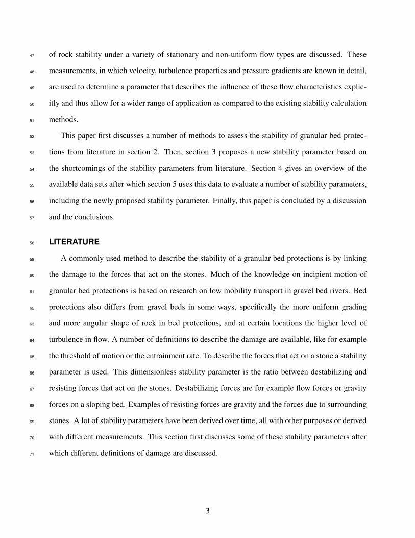
of rock stability under a variety of stationary and non-uniform flow types are discussed. These47

measurements, in which velocity, turbulence properties and pressure gradients are known in detail,48

are used to determine a parameter that describes the influence of these flow characteristics explic-49

itly and thus allow for a wider range of application as compared to the existing stability calculation50

methods.51

This paper first discusses a number of methods to assess the stability of granular bed protec-52

tions from literature in section 2. Then, section 3 proposes a new stability parameter based on53

the shortcomings of the stability parameters from literature. Section 4 gives an overview of the54

available data sets after which section 5 uses this data to evaluate a number of stability parameters,55

including the newly proposed stability parameter. Finally, this paper is concluded by a discussion56

and the conclusions.57

LITERATURE58

A commonly used method to describe the stability of a granular bed protections is by linking59

the damage to the forces that act on the stones. Much of the knowledge on incipient motion of60

granular bed protections is based on research on low mobility transport in gravel bed rivers. Bed61

protections also differs from gravel beds in some ways, specifically the more uniform grading62

and more angular shape of rock in bed protections, and at certain locations the higher level of63

turbulence in flow. A number of definitions to describe the damage are available, like for example64

the threshold of motion or the entrainment rate. To describe the forces that act on a stone a stability65

parameter is used. This dimensionless stability parameter is the ratio between destabilizing and66

resisting forces that act on the stones. Destabilizing forces are for example flow forces or gravity67

forces on a sloping bed. Examples of resisting forces are gravity and the forces due to surrounding68

stones. A lot of stability parameters have been derived over time, all with other purposes or derived69

with different measurements. This section first discusses some of these stability parameters after70

which different definitions of damage are discussed.71

3

Stability parameters for uniform flow72

One of the most well-known stability parameters is the one proposed by Shields (1936). See73

also the reviews of Buffington (1999), and Dey and Papanicolaou (2008). Shields (1936) assumed74

that the stability of a stone on the bed is determined by the bed shear stress τb and the submerged75

weight of the stones:76

ΨS =τb

(ρs − ρw)gd=

u2τ∆gd

(1)77

With τb the bed shear stress, uτ the friction velocity,∆ the relative stone density (∆ = (ρs −78

ρw)/ρs), ρs the mass density of the stones [kg/m3], ρw the mass density of water, g the gravitational79

acceleration and d the stone diameter [m]. A similar stability parameter was introduced by Izbash80

(1935). In this parameter the numerator represents the square of the (local) mean velocity instead81

of the shear velocity.82

The Shields parameter is derived for uniform flow and is therefore strictly speaking not applica-83

ble to non-uniform flow. It is possible to include the effects of turbulence in the Shields parameter84

by using an influence factor, see e.g. Schiereck (2001). These influence factors are often empirical85

relations based on specific flow situations resulting in a wide range of influence factors, lacking86

general validity. For every new or unknown situation, a new relation for the influence factor has to87

be derived. Another drawback is that the Shields parameter cannot predict the initiation of motion88

at locations with zero mean velocity but large fluctuations, like in reattachment points behind a89

backward-facing step.90

91

Influence of the bed slope92

The slope of the bed influences the initiation of motion of the rocks. Based on the force balance93

on a particle, the change in critical shear stress can be incorporated in a stability parameter. For a94

longitudinal bed slope this factor reads (Chiew and Parker 1994):95

4

Kβ =φ− βsin(φ)

(2)96

With φ the angle of repose of the rocks and β the angle of the longitudinal slope. This relation is97

also used for bed protections (Schiereck 2001) A more general equation for the influence of a both98

longitudinal and transversal slope is also derived (Dey 2003, for example). In the present study99

only longitudinal slopes were considered.100

101

Stability parameters with explicit incorporation of turbulence102

Jongeling et al. (2003) propose a method that takes the turbulence into account more explicitly.103

The flow force (numerator) in this stability parameter is a combination of velocity and turbulence104

evaluated in the water layer above the location where the bed stability is regarded. The effect of105

turbulence is calculated as the square root of the turbulent kinetic energy k times an empirical106

turbulence magnification factor α. In this and the following stability parameters the stone diameter107

d is represented by dn50, the nominal diameter (equivalent cube size) that is exceeded by 50% of108

the total mass of the stones.109

Hofland (2005) proposed a similar stability parameter based on the assumption that large-scale110

velocity fluctuations can reach the bottom via an eddying motion. The large-scale velocity fluctu-111

ations at height z are assumed to be proportional to the square root of the turbulent kinetic energy112

√k. The fluctuations are part of a large rolling eddy so that the ’maximum velocity’ at the bed can113

be determined using a length scale. The maximum of the local instantaneous velocity (u + α√k)114

at a certain height z is weighed with the relative mixing length Lm/z, since it is likely that the115

turbulent sources higher in the water column have less influence on the bed. Subsequently, the116

moving average with varying filter length Lm is taken of the weighted maximum velocity. Hofland117

(2005) found that using the Bahkmetev mixing length distribution lm leads to the best results. The118

Hofland stability parameter is described in equation 3.119

5

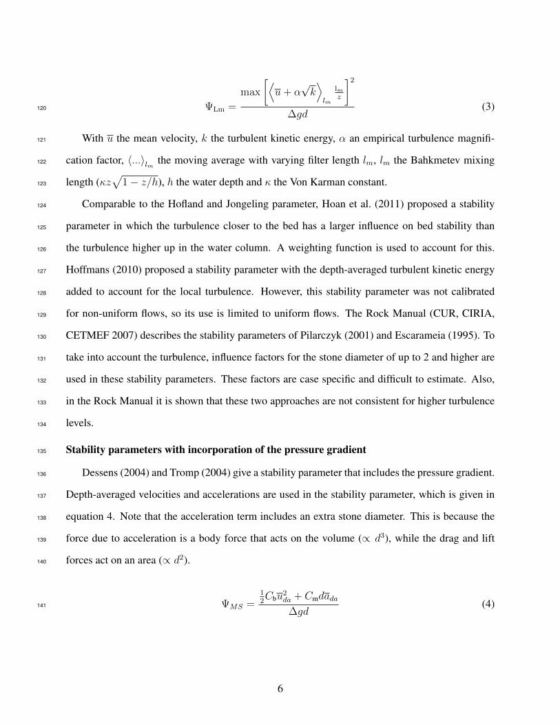
ΨLm =

max

[⟨u+ α

√k⟩lm

lmz

]2∆gd

(3)120

With u the mean velocity, k the turbulent kinetic energy, α an empirical turbulence magnifi-121

cation factor, 〈...〉lm the moving average with varying filter length lm, lm the Bahkmetev mixing122

length (κz√

1− z/h), h the water depth and κ the Von Karman constant.123

Comparable to the Hofland and Jongeling parameter, Hoan et al. (2011) proposed a stability124

parameter in which the turbulence closer to the bed has a larger influence on bed stability than125

the turbulence higher up in the water column. A weighting function is used to account for this.126

Hoffmans (2010) proposed a stability parameter with the depth-averaged turbulent kinetic energy127

added to account for the local turbulence. However, this stability parameter was not calibrated128

for non-uniform flows, so its use is limited to uniform flows. The Rock Manual (CUR, CIRIA,129

CETMEF 2007) describes the stability parameters of Pilarczyk (2001) and Escarameia (1995). To130

take into account the turbulence, influence factors for the stone diameter of up to 2 and higher are131

used in these stability parameters. These factors are case specific and difficult to estimate. Also,132

in the Rock Manual it is shown that these two approaches are not consistent for higher turbulence133

levels.134

Stability parameters with incorporation of the pressure gradient135

Dessens (2004) and Tromp (2004) give a stability parameter that includes the pressure gradient.136

Depth-averaged velocities and accelerations are used in the stability parameter, which is given in137

equation 4. Note that the acceleration term includes an extra stone diameter. This is because the138

force due to acceleration is a body force that acts on the volume (∝ d3), while the drag and lift139

forces act on an area (∝ d2).140

ΨMS =12Cbu

2da + Cmdada

∆gd(4)141

6

With uda the mean depth-averaged velocity, ada the mean depth-averaged acceleration, Cb the142

combined drag and lift coefficient and Cm the added mass coefficient.143

Dessens (2004) studied stationary acceleration in a contraction while Tromp (2004) studied144

time-dependent acceleration in waves. Dessens (2004) found values for Cb of 0.10 to 0.14 and for145

Cm of 3.9 to 5.6.146

Damage147

There are a number of methods available in theory to assess the stability of granular bed pro-148

tections. The most well-known are the threshold of motion and the stone transport concept. In the149

first concept it is assumed that there is a certain condition at which incipient motion occurs and150

that stones start to move when this condition is exceeded. A critical value of the stability parameter151

is derived from measurements and used in the design of bed protections. The most well-known152

method that uses this concept is the one of Shields (1936). Jongeling et al. (2003) also gives a153

method that uses the threshold of motion in the design of bed protections.154

The condition at which the threshold of motion occurs is rather subjective, since movement155

of stones can be interpreted in different ways. To partly overcome this problem, Breusers and156

Schukking (1971) defined 7 transport stages that go from no movement at all to general transport157

of the grains. Because of the irregularities in natural stones, the exposure of the stones and the158

irregular deviations from the mean flow characteristics due to turbulence, one general threshold of159

motion for the entire bed does not exist. Another disadvantage of the threshold of motion method,160

is that there is no information about the behaviour of the bed when the critical stability parameter is161

exceeded. This makes this method not usable for the design of for example maintenance programs162

for bed protections.163

Another way to describe the stability of granular bed protections is in terms of stone transport.164

Here, the flow forces acting on the stones (written as a stability parameter Ψ) are linked to the bed165

response (as a dimensionless transport indicator Φ). The main advantage of this method is that it166

describes the behaviour of the bed after it becomes unstable. The general form of this relation is167

Φ = f(Ψ).168

7

The dimensionless transport parameter Φ should represent the damage to the bed properly. Two169

ways of defining the transport of particles are distinguished. First there is the (volume) entrainment170

rate, this is the number of pick-ups per unit time and area. Second, the bed load transport can be171

used. This is the number of particles that is transported through a cross-section per unit time.172

Paintal (1971) provided a formula for low-mobility transport rates, also for dimensionless shear173

stresses under the ‘critical’ value of Ψ = 0.05.174

Hofland (2005) states that because of the dependence of the bed load transport on upstream175

hydraulics (the stones passing a certain cross-section is a function of all the entrained stones up-176

stream) the bed load transport is a non-local parameter. The entrainment rate, however, is com-177

pletely dependent on local hydrodynamic parameters. The stability parameter Ψ also is a local178

parameter (solely depending on local flow characteristics). Hence here the entrainment rate is used179

to define and quantify the stability of the bed. The time dependence should be included in the180

entrainment rate, because due to turbulent fluctuations a stone moves sporadically and thus more181

stones are entrained during a longer period of time. The (volume) entrainment rate is described by182

equation 5.183

E =nd3

AT(5)184

In which E is entrainment rate, n the number of stones picked up, d the stone diameter, A the185

surface area and T the duration.186

To describe the relation between the dimensionless transport parameter Φ and the stability187

parameter Ψ, often a power-law is used. The relation found by Hofland (2005) by using data188

from Jongeling et al. (2003) and De Gunst (1999) is shown in 1. The assumption was made that189

the initiation of motion is best described by a stability parameter where the correlation between a190

stability parameter Ψ and the dimensionless entrainment rate ΦE is largest. This method is also191

applied presently. For a large variety of flow types the coefficients in the stability parameter are192

chosen such that the maximum correlation between Ψ and ΦE is found.193

8

PROPOSED STABILITY PARAMETER194

In this paper, a new stability parameter is proposed that combines the effects caused by turbu-195

lence and the effects caused by the pressure gradient in stationary accelerating flows. The Hofland196

parameter is used for the influence of the velocity and turbulence and a pressure gradient is added197

to this parameter. The pressure gradient in accelerating flow can be approximated in different198

ways. Froehlich (1997) uses an expression based on buoyancy force that results from a water level199

gradient. Hofland (2005), Dessens (2004) and Huijsmans (2006) use an aproximation based on the200

Euler equation, which states that ax ≈ − ∂p∂x

. Hence, building upon the expression in equation 3 the201

newly proposed stability parameter is given by equation 6, now including a pressure term.202

Ψ∗new

Cb=

(max

[⟨u+ α

√k⟩Lm

Lm

z

]2)− Cm/Cb

dpdxd

Kβ∆gd(6)203

In this equation, k is the turbulent kinetic energy, Lm the Bakmetev mixing length, z the height204

above the bed, u the mean (i.e. time-averaged) velocity, d the nominal stone diameter, dn50, Kβ205

the correction for the bed slope in the flow direction.206

In the proposed stability parameter, the following three unknowns are present:207

208

Cb the bulk coefficient. Representing the relative importance of the force caused by

velocity and turbulent velocity fluctuations. This parameter is a combination of

the effects due to the drag, lift and shear forces.

α an empirical turbulence magnification factor. This is the value of the turbulent

velocity fluctuations represented by√k relative to the mean velocity.

Cm the added mass coefficient. This coefficient represents the force caused by the

pressure gradient relative to the force due to the quasi steady forces.

209

210

The remainder of this article focuses on finding the unknowns in equation 6 and formulating211

an equation that predicts the dimensionless entrainment rate as function of the new dimensionless212

stability parameter. The relation that is used is a power law of the form ΦE = a · Ψbnew. The213

9

unknowns are found by means of a correlation analysis. Further on, the unknowns Cm and Cb will214

be combined into one parameter Cm/Cb and the new stability parameter Ψnew will be defined as215

Ψ∗new/Cb. Measurements of flow characteristics (velocity, turbulent kinetic energy and pressure216

gradient) are coupled to the simultaneously measured entrainment rate. Before the correlation217

analysis is discussed, the next section first mentions the available data sets after which an evaluation218

is made on the usability of each data set.219

DATA220

This section discusses the data sets that are used in this paper. The data sets represent mea-221

surements of initiation of motion of coarse, angular bed material (hydraulically rough beds) under222

low transport conditions (entrainment rates corresponding to values of the Shields parameter well223

under the critical Shields factor for transport), and with detailed velocity measurements in the ver-224

tical above the location where the stone entrainment has been measured. As stone entrainment and225

the flow characteristics are measured at several locations for a single test setup, several data points,226

with varying mean flow, turbulence and acceleration characteristics are typically obtained for one227

flow configuration. This section first describes the data sets that have been used, after which an228

evaluation is made on the possibility to use the data sets in this research.229

Data Used230

The data that have been used are obtained at Deltares and the Delft University of Technology231

over the last decade. As not all data has been published yet in peer-reviewed journals, much of the232

data is re-analyzed presently. Table 1 summarizes the measurements that have been used in this233

paper.234

Jongeling data235

Jongeling et al. (2003) did measurements in a flume at Deltares with a length of 23 m, a width236

of 0.50 m and a height of 0.70 m for the following flow configurations, i.e.:237

• Flow over a flat bed;238

• Flow over a sill with a short crest;239

10

• Flow over a sill with a long crest;240

Bed material was used with a stone diameter of dn50 = 0.062 m, a grading width of dn85/dn15 =241

1.51, and a submerged relative density of ∆ = 1.72. This was applied in a 4 cm thick layer on the242

flume floor. The bed was divided in coloured strips of 0.1 m length.243

For the flat bed case, measurements were done over a 5.6 m long section, which was located244

behind a 13.6 long roughened initial section, to create uniform flow conditions. Water depths of245

about 0.25, 0.375, and 0.5 m were applied, with corresponding bulk mean velocities of respectively246

0.7, 0.63 and 0.68 m/s. The short sill had an upstream slope and downstream slope of 1:8, a crest247

height of 0.12 m, and a crest width of 0.1 m. Measurements were made on the upstream slope248

(1 location), crest (2 locations), downstream slope (1 location), and downstream of the sill (6249

locations). The long sill had an upstream slope of 1:8 and a downstream slope of 1:3, a crest height250

of 0.12 m, and a crest width of 2 m. Measurements were done on the crest (2 locations), and251

downstream of the sill (8 locations).252

The velocity was measured by a combination of a 6 mW, forward scatter, Laser Doppler Ve-253

locimeter (LDV) and an Electro Magnetic velocity Sensor (EMS). The LDV measured the stream-254

wise (u) and vertical (w) velocity components in a measurement volume with a 1 mm diameter255

and 10 mm transversal length, and the EMS measured the streamwise and transversal (v) velocity256

components in a roughly 1*1*1 cm measuring volume. The EMS measures a lower energy content257

as the velocity is averaged over a larger area, therefore k was determined by using the LDV results258

for the u and w components, and to correct v measured by the EMS by the ratio of the standard259

deviations of the longitudinal velocity components of LDV and EMS, σ(uLDV )/σ(yEMS).260

The discharge was measured by an electromagnetic device in the return flow, and the water261

levels were measured by a resistive type gauge.262

The velocity was measured at different heights at a number of locations in the length of the263

flume, leading to a number of velocity profiles with their corresponding bed response. The stones264

at the bed that were located in a certain strip and had a certain colour. In this way, one could count265

how many stones moved and from what strips they originated. It should be mentioned that stones266

11

that move within their own strip are neglected when this method is used. Hofland (2005) suggested267

a correction factor for this, based on the probability distribution of the displacement length of the268

stones (see appendix D in Hofland (2005)). This correction is used on all the counted stones in this269

research.270

Hoan data271

Hoan et al. (2011) investigated the effect of increased turbulence on stone stability by analyz-272

ing measurements in an open-channel flow with symmetric, gradually expanding side walls in a273

laboratory flume. The flow width increased from 0.35 to 0.50 m. Three different expansions (3◦, 5◦274

and 7◦ for both side walls) were used to create different combinations of velocity and turbulence.275

No flow separation occurred at the side walls. Just as for the Jongeling data, flow velocities and276

the number of picked-up stones are measured.277

The measurements were carried out at the Delft University of Technology in a flume with a278

width of 0.50 m and a height of 0.70 m. For the flow conditions a similar type of LDV was279

used. As only two velocity components (u and w) are available, the turbulence kinetic energy was280

approximated by assuming that σ(v) = σ(u)/1.9. The discharge was measured using an orifice281

plate in the inflow pipe.282

Angular stones having a density of 2.700 kg/m3, a nominal diameter of dn50 = 0.08 m, and283

dn85/dn15 = 1.27 were placed at the horizontal flume bottom. The flow velocity during the experi-284

ments was too low to displace these natural stones. To examine stone stability, the top two layers285

of rock were replaced by uniformly coloured strips of artificial light stones at designated locations286

(0.1 m long by 0.2 m wide) on the flume axis before and along the expansion. These artificial287

stones were made of epoxy resin with densities in the range of 1,320 to 1,971 kg/m3, mimicking288

shapes and sizes of natural stones. They had a nominal diameter of dn50 = 0.082 m and dn85 /dn15289

= 1.11.290

Dessens and Huijsmans data291

Dessens (2004) and Huijsmans (2006) both investigated the effect of stone stability in acceler-292

ating flow by doing measurements in the same type of configuration. The same flume as in Hoan293

12

et al. (2011) was used, and a local contraction was created. Both used the same measurement294

instruments as Jongeling et al. (2003) and measured velocities, water levels and discharges. The295

stone transport was measured in the same way as Hoan et al. (2011). Different contraction angles296

were used, creating different combinations of velocities and accelerations.297

Stones with a density of 2.680 kg/m3 and two different stone sizes were used. One with a nomi-298

nal diameter of dn50 = 0.02 m and the other with dn50 = 0.0082 m. The last 0.40 m of the contraction299

was covered with 0.10 m wide strips of coloured stones to measure the stone entrainment.300

Discussion of the data sets301

To be able to evaluate the parameters, the data sets have to contain the following information:302

• velocity;303

• turbulent kinetic energy;304

• pressure gradient (or the stationary acceleration);305

• entrainment rate.306

The data sets of Hoan (2008), Dessens (2004) and Huijsmans (2006) can directly be used307

for the purposes of this article. In these data sets the pressure gradient was obtained from the308

measured free-surface slope. The data set of Jongeling et al. (2003), however, did not contain309

enough information for determining the pressure gradient dp/dx. Hence, a numerical model was310

created to determine the missing dp/dx at several measurements. The open source numerical311

solver OpenFOAM version 1.6-ext, see OpenFOAM Foundation (2012), has been used for this312

(Steenstra 2014).313

Besides the additional numerical calculations for the Jongeling et al. (2003) data, the measured314

mean velocity and turbulence kinetic energy for all the different data sets have been calculated315

anew from the raw measurement data using the same processing script, in order to assure a uniform316

processing method.317

ANALYSIS318

13

The previous section discussed the data sets that are used in this research. These measurements319

will now be used to calculate a number of existing stability parameters and plot them against the320

measured dimensionless entrainment rate. After that, the unknowns in the proposed new stability321

parameter are determined by means of a correlation analysis. When these unknowns are deter-322

mined, an analysis of the performance of the new stability parameter is made.323

Existing stability parameters324

Below, the measurements are used to calculate the Shields parameter, the Hofland parameter325

and the Dessens parameter. These parameters are subsequently plotted against the dimensionless326

entrainment rate derived from the measurements327

Shields parameter328

Figure 2 shows the Shields parameter plotted against the dimensionless entrainment rate. The329

shear stress velocity uτ is calculated with equation 7 at the first data point located at a level z1330

above the bed.331

uτ =u · κ

ln 15·z1(dn50)

(7)332

The coefficient of determination R2 (obtained through lineair regression) is 0.24 showing that333

much scatter is present. Especially the higher turbulence data points (like the long sill, short sill334

and the expansion) show a large deviation from the other data points.335

For the flat bed only a few cases are included in the data sets. For these cases, the relationship336

between ΨS and ΦE appears approximately linear (on the log-log scale). It can be seen that the337

data represent very low mobility with values of ΨS between 0.02 and 0.03, which is well below the338

initiation of motion criterion of Shields of 0.055. It is also still just below the first of 7 stages of in-339

creasing bed mobility: ”displacement of grains, once in a while”, which coincides with ΨS ≈ 0.03340

for coarse grains (Breusers and Schukking 1971), but within the range of low-mobility transport341

as measured by Paintal (1971).342

Along the contraction the shear stress gets larger. According to the Shields parameter the bed343

14

shear stress is a destabilizing force and increasing bed shear stress causes increasing entrainment.344

Figure 2 clearly shows this behaviour in the accelerating flow (contraction) where for the same345

contraction, the entrainment rate increases with increasing Shields parameter. However, the data346

points in a contraction with a small side wall angle have, for equal entrainment, a larger ΨS than347

the contraction with a larger angle, indicating that the effect of acceleration itself (aside from348

the increased bed shear stress in accelerating flow) is not incorporated correctly in the Shields349

parameter.350

For the expansion case with decelerating flow, very low correlation is seen between ΨS and ΦE .351

Because of the decreased (shear) velocity in decelerating flow, ΨS decreases in decelerating flow352

and a decreasing entrainment rate would be expected. Figure 2 shows totally different behaviour.353

The entrainment rate in decelerating flow is rather uncorrelated to the Shields parameter. This354

can be attributed mainly to the absence of explicit incorporation of the turbulence in the Shields355

parameter.356

The above shows that the bed shear stress is not a sufficient measure for predicting the damage357

to bed protections in non-uniform stationary flows.358

Hofland parameter359

The next existing stability parameter that is evaluated is the stability parameter ΨLm from360

Hofland (2005).The parameter ΨLm is defined in equation 3. Both Hofland and Booij (2006) and361

Hoan et al. (2011) determined the coefficients in this parameter. Hofland and Booij (2006) used362

the Jongeling et al. (2003) data set and found a value for the turbulence influence factor α of 6.0.363

Hoan et al. (2011) used his data of the expanding flows and found an α of 3.0. A relation between364

ΨLm and ΦE , using the values for the constants as derived by Hofland and Booij (2006), is plotted365

in figure 3. Using the constants as fitted by Hoan yields a similar graph.366

The data points with relatively high turbulence and the data points of the flat bed simulation367

collapse well. The data points from the configurations with high accelerations show, for equal368

ΨLm, much higher entrainment rates than those of the other cases, indicating that the entrainment369

rate is influenced by the pressure gradient in acceleration flows.370

15

The Hofland stability parameter ΨLm was designed to incorporate the effects of turbulence ex-371

plicitly. Figure 3 shows that the parameter does this correctly, also for the newer data of Hoan et al.372

(2011). This confirms the findings of Hofland (2005), in which the behaviour of ΨLm was anal-373

ysed more extensive for the configurations of Jongeling et al. (2003). However, for the data points374

with a larger acceleration ΨLm does not predict the entrainment rate accurately. Both Hofland375

(2005) and Hoan (2008) parameters will underestimate the entrainment in the contractions. This376

underestimation is attributed to the direct destabilizing effects of the pressure gradient on the stone377

stability.378

Dessens parameter379

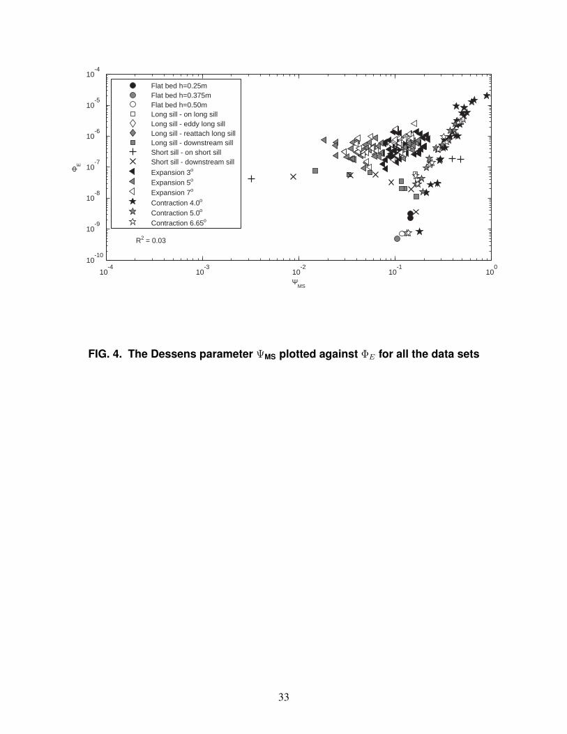
Figure 4 shows the stability parameter proposed in Dessens (2004) (equation 4) plotted against380

the dimensionless entrainment rate. Remember that the effect of turbulence is not incorporated381

explicitely in this equation.382

Figure 4 shows that using ΨMS leads to even larger scatter than using the Shields parameter383

ΨS . The value of R2 is 0.028 for the entire set of used data in this article. This is almost a factor384

10 smaller than the R2 from the Shields parameter.385

In contrast to figure 2, the contraction data points collapse well, which is not a coincidence386

because these are the data sets for which ΨMS was derived. The flat bed and part of the sill data387

points also collapse onto these data.388

The measurement points that had high turbulence deviate a lot from the data points of the389

contraction. For these data points the entrainment rate is highly underestimated by the relation390

of Dessens (2004), which is derived for relatively small turbulence. The entrainment rate in the391

expansion shows almost no correlation with the stability parameter. The fact that these data points392

deviate from the trend for the accelerating flows can be explained by the fact that Dessens (2004)393

did not use an explicit formulation for the turbulence. Hence the influence of the turbulence was394

implicitly added to the drag/lift coefficient Cb. This ratio is apparently only applicable for the395

contraction and the flat bed cases.396

The Dessens stability parameter ΨMS performs reasonably for situations with relatively small397

16

turbulence, such as in uniform or accelerating flows. As soon as there is increased turbulence, and398

there is no correction formula present for the change in relative turbulence, ΨMS does not predict399

the bed damage correctly at all.400

Evaluation of the new stability parameter401

The unknowns in equation 6 are determined by finding the combination of unknowns that402

lead to the highest correlation between the calculated stability parameter and the dimensionless403

entrainment rate. To minimize the number of unknowns it is chosen to combine the constants Cb404

and Cm into only one constant (see equation 8) and to define Ψnew as Ψ∗new/Cb.405

Cm:b =Cm

Cb(8)406

Instead of the absolute value of Cb and Cm, now just the ratio between the two is calculated.407

For establishing a relation between Ψnew and ΦE , this is sufficient.408

The steps that are taken in the correlation analysis are:409

1. Set values for α, Cm:b410

2. Calculate Ψnew with equation 6411

3. Find a and b in ΦE = aΨb through linear regression412

4. Calculate the coefficient of determination R2 = 1−∑(

ΦE − aΨbnew

)2/∑(

ΦE − ΦE

)2413

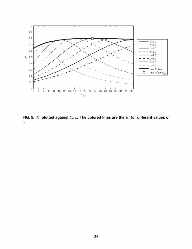
5. Repeat steps 1 to 5 for a number of values of α and Cm:b414

For α values of 0 to 7, with a step of 0.25 have been used. For Cm:b values of 0 to 40, with a415

step of 1.0 have been used. Executing the method described above leads to the correlations shown416

in figure 5. The thick black line indicates the local maximum of R2 for every Cm:b. The square417

dot indicates to absolute maximum with a R2 of 0.80 with α = 3.75 and Cm:b = 23. However,418

it should be mentioned that for values of Cm:b larger than approximately 15.0 (and α = 3.0), the419

value of R2 remains approximately equal, with values around 0.79.420

Equation 9 gives the final definition of the stability parameter Ψnew. The first term in the421

17

nominator includes the forces that are caused by the velocity and the turbulent fluctuations that422

reach the bed. The second term accounts for the force caused by the pressure gradient due to423

acceleration.424

Ψnew ≡

(max

[⟨u+ α

√k⟩Lm

Lm

z

]2)− Cm:b

dpdxdn50

Kβ ·∆gdn50(9)425

The values for a and b in the power law ΦE = aΨbnew result from the regression analysis.426

Equation 6 gives the relation between the stability parameter and the bed response. The plot of this427

relation and the associated data points are given in figure 6.428

The relation between the new stability parameter Ψnew (for α = 6 and Cm:b = 23) and the429

dimensionless entrainment rate ΦE is given in equation 10 and plotted in figure 6 on log-log scale,430

and in figure 7 on a semi-log scale.431

ΦE ≡ 3.95 · 10−9Ψ5.89new for 0.9 < Ψnew < 4.3 (10)432

Table 2 gives some statistical quantities that followed from the regression analysis. These433

quantities can be used in for example probabilistic calculations. In the table the mean and standard434

deviation of the constants in ΦE = aΨb are given. Note that the a in this equation is not the435

acceleration.436

From the analysis of the existing stability parameters it followed that the existing stability437

parameters were correlated to the dimensionless entrainment rate for the type of flow they were438

developed for, but that they did not perform for other types of stationary flows. The proposed439

new stability parameter Ψnew from equation 10 includes, besides the influence of the mean flow440

velocity, both the influence of the (mean) pressure gradient as well as the explicitly described441

influence of the turbulence.442

The correlation parameter for the relation between the Hofland stability parameter ΨLm (with443

18

α = 3.0 and Cm:b = 0) and ΦE , for the selected data sets, was 0.27. Using Ψnew (with α = 3.75444

and Cm:b = 23.0 leads to a R2 of 0.80. For the data sets used in this research, adding the effects of445

the pressure gradient in accelerating flow gives a considerable increase in correlation.446

Table 3 gives the values for Cb and Cm from other sources. The value from ”theory” is based on447

the classic case of a sphere in a uniform flow. Here the drag coefficient is 0.4 (or somewhat higher448

if it is a blunt body) and the inertia coefficient is 2.0, such that Cm:b = 5.0. This value can change449

with the shape of the rocks, but still seems rather small. This difference can be explained by the450

fact that the drag only acts on the top part of the rock (typically the rocks protrude 20% from the451

theoretical bed level), while the pressure gradient penetrates the bed to a much larger extent. This452

could make the relative influence of the inertia in the order of five times larger, which will yield453

values of Cm:b in the same order as those found in the correlation analysis.454

The value of Cm:b = 23.0 is roughly the average of the values found by Dessens (2004) and455

Tromp (2004). It also seems to be in the order of theoretical values. For now it is concluded that456

Cm:b = 23.0 is a plausible value for Cm:b because it is within the rangeof previously found values457

and it predicts the effects of acceleration correctly in the stability parameter.458

However, it should be mentioned that for values with a Cm:b larger than 15.0, and their cor-459

responding smaller α, the correlation remains approximately equal. Choosing a smaller Cm:b and460

thus a smaller α can lead to less uncertainty in stability calculations since α√k is usually a large461

uncertainty if the output from a numerical model is used.462

463

An example calculation from Steenstra (2014) shows that in the contraction (with most notable464

pressure gradient) the acceleration term increased the required rock size by approximately a factor465

2 (so the weight by a factor 8). Contrary to this, in cases with decelerating flow the calculated466

rock size will be smaller when Ψnew is used because the stabilizing effect of the adverse pressure467

gradient is included. This indicates that the acceleration has a significant influence on the required468

rock size in practice.469

470

19

For design purposes a fixed value of ΦE might be used as ‘critical’ value. For a uniform flow471

the ΦE corresponding to a critical Shields factor of Ψ ≈ 0.03, is ΦE ≈ 10−8 (Hofland 2005), see472

figure 2. According to figure 6 this corresponds to a value of the new parameter of Ψnew,c ≈ 1.2.473

DISCUSSION474

Some possible inaccuracies and limitations of the method are discussed next. A force gen-475

erating mechanism that is not included in Ψnew are the turbulent wall pressures. Turbulent wall476

pressures (i.e. fluctuating accelerations due to turbulence) can also entrain stones (Hofland 2005;477

Smart and Habersack 2007). This effect is not included explicitly in the stability parameter.478

The entrainment rate is prone to scatter, as only several stones move per experiment, and the trans-479

port within a coloured strip has to be estimated. Moreover, the advective acceleration is used as480

approximation for the pressure gradient over the stone. This approximation can introduce errors.481

Including both the effects of turbulence and the pressure gradient in the stability parameter482

greatly increases the range of application of the stability parameter compared to the already existing483

ones. However, the proposed stability parameter and its relation with the bed response is derived484

only for stationary acceleration. The effect of time-dependent acceleration (e.g. waves) should be485

investigated further before the proposed formulation can be used for that case. In wave action the486

value of the coefficient becomes a function of the wave period (acceleration period).487

CONCLUSIONS488

The stability of stones in bed protections is influenced by the quasi-steady forces, turbulent wall489

pressures and pressure gradients due to acceleration. Existing stability assessment methods do not490

incorporate all of these forces and are usually derived for only part of these forces. In this paper, a491

stability parameter is proposed that includes the influence of the mean flow velocity, turbulence and492

stationary acceleration in equation 9. Measurements of stone entrainment in a wide range of flow493

conditions and geometries are used to calibrate the constants in the proposed stability parameter.494

Missing data on pressure gradients were reconstructed by means of a computational model in the495

software package OpenFOAM.496

20

The performance of several existing stability parameters was checked. It can be concluded497

that these parameters mainly can be used to obtain a relation between the stability parameter and498

the dimensionless entrainment rate (i.e. predict damage) for the flow type for which they were499

developed.500

The proposed stability parameter Ψnew shows the right behaviour for uniform, accelerating and501

decelerating flow, and thus has a wider range of application than the investigated existing stability502

parameters. The values of the derived α and Cm:b are within the range of values that are derived503

in earlier research.A maximal correlation was obtained for α = 3.75 and Cm:b = 23. The newly504

proposed stability parameter Ψnew can be used in the design of bed protections to recognize the505

areas where larger (or smaller) stones are required, which can result in more efficient design of bed506

protections.507

21

APPENDIX I. REFERENCES508

Breusers, H. and Schukking, W. (1971). “Initiation of motion of bed material.” Tech. rept. S 151-1,509

Deltares | Delft Hydraulics. (In Dutch).510

Buffington, J. (1999). “The legend of A.F. Shields.” J. Hydraul. Eng, 125(4), 376–387.511

Chiew, Y. M. and Parker, G. (1994). “Incipient sediment motion on non-horizontal slopes.” J.512

Hydraul. Res., 32(5), 649 – 660.513

CUR, CIRIA, CETMEF (2007). The Rock Manual: The use of rock in hydraulic engineering.514

London, 2nd edition.515

De Gunst, M. (1999). “Stone stability in a turbulent flow behind a step.” M.Sc. thesis. Delft Uni-516

versity of Technology (In Dutch).517

Dean, R. G. and Dalrymple, R. A. (1991.). Water wave mechanics for engineers and scientists.518

Singapore: World Scientific Publishing Co. Pte. Ltd.519

Dessens, M. (2004). “The influence of flow acceleration on stone stability.” M.Sc. thesis.520

Delft University of Technology, http://data.3tu.nl/repository/uuid:0ba04590-0c47-4e0c-80eb-521

979b2cc08e0c.522

Dey, S. (2003). “Threshold of sediment motion on combined transverse and longitudinal sloping523

beds.” J. Hydraul. Res., 41(4), 405 – 415.524

Dey, S. and Papanicolaou, A. (2008). “Sediment threshold under stream flow: A state-of-the-art525

review.” ASCE Journal of Civil Engineering, 12(1), 45 – 60.526

Escarameia, M. & May, R. W. P. (1995). “Stability of riprap and concrete blocks in highly turbulent527

flows..” Proc. Instn Civ. Engrs Wat. Marit. & Energy, (112), 227237.528

Froehlich, D. C. (1997). “Riprap particle stability by moment analysis.” Proc. 27th congress of the529

IAHR, San Francisco.530

Hoan, N. T. (2008). “Stone stability under non-uniform flow.” Ph.D. thesis. Delft Univerisity of531

Technology. http://data.3tu.nl/repository/uuid:cca1e773-4c36-4aa4-9ef7-38c86a0ed20e.532

Hoan, N. T., Stive, M. J. F., Booij, R., and Verhagen, H. J. (2011). “Stone stability in non-uniform533

flow.” J. Hydraul. Eng, 137(9).534

22

Hoefel, F. and Elgar, S. (2003). “Wave-induced sediment transport and sandbar migration.” Sci-535

ence, 299, 1885.536

Hoffmans, G. (2010). “Stability of stones under uniform flow.” J. Hydraul. Eng, 136(2), 129–136.537

Hofland, B. (2005). “Rock & roll; turbulence-induced damage to granular bed protections”. Ph.D.538

thesis. Delft University of Technology.539

Hofland, B. and Booij, R. (2006). “Numerical modeling of damage to scour protections.” Third540

International Conference on Scour and Erosion, Amsterdam, The Netherlands.541

Huijsmans, M. A. (2006). “The influence of flow acceleration on the stability of stones.” M.Sc.542

thesis. Delft University of Technology, http://data.3tu.nl/repository/uuid:6bd3d2b8-07e9-4742-543

a6fb-c78179c6a476.544

Izbash, S. V. (1935). “Constructions of dams by dumping of stone in running water. Moscow,545

Leningrad.546

Jongeling, T. H. G., Blom, A., Jagers, H. R. A., Stolker, C., and Verheij, H. J. (2003). “Design547

method granular protections.” Report No. Q2933 / Q3018, WL | Delft Hydraulics. (december).548

In Dutch.549

Jongeling, T. H. G., Jagers, H. R. A., and Stolker, C. (2006). “Design of granular bed protections550

using a RANS 3D-flow model.” Third International Conference on Scour and Erosion, Amster-551

dam, The Netherlands.552

Maynord, S. T., Ruff, J. F., and Abt, S. R. (1989). “Riprap design.” Journal of Hydraulic Engineer-553

ing, 115(7), 937–949.554

OpenFOAM Foundation (2012). OpenFOAM: The Open Source CFD Tool User Guide, version555

2.1.1 edition (May).556

Paintal, A. S. (1971). “Concept of critical shear stress in loose boundary open channels.” Journal557

of Hydraulic Research, 9, 91113.558

Pilarczyk, K. W. (2001). “Unification of stability formulae for revetments.” XXIX IAHR congress559

(September).560

Schiereck, G. J. (2001). Introduction to bed, bank and shore protection. VSSD, Delft.561

23

Shields, A. (1936). “Anwendung der aehnlichkeitsmechanik und der turbulenzforschung auf die562

geschiebebewegung.” Mitteilungen der Preussischen Versuchsanstalt fuer Wasserbau und Schiff-563

bau. Berlin, Germany.564

Smart, G. M. and Habersack, H. M. (2007). “Pressure fluctuations and gravel entraiment in rivers.”565

J. Hydraul. Res., 45(5), 661 – 673.566

Steenstra, R. S. (2014). “Incorporation of the effects of accelerating flow in the design of granular567

bed protections.” M.Sc. thesis. Delft University of Technology.568

Tromp, M. (2004). “The influence that fluid accelerations have on the threshold of motion.” M.Sc.569

thesis. Delft University of Technology.570

24

List of Tables571

1 Summary of the measurements that have been used in this paper . . . . . . . . . . 26572

2 Statistical quantities of the relation in equation 9 . . . . . . . . . . . . . . . . . . . 27573

3 Values for Cm/Cb from other sources. . . . . . . . . . . . . . . . . . . . . . . . . 28574

25

So

urc

e

Co

nfi

gu

rati

on

Na

me

h [

m]

Q [

l/s]

No

. o

f

dif

fere

nt

Q a

nd

h

Me

asu

rem

en

t

loca

tio

n

No

. o

f

me

asu

rem

en

t

loca

tio

ns

No

. o

f

me

asu

rem

en

t

po

ints

ov

er

de

pth

Be

d s

lop

e

i

[-]

Wid

th

[m]

Sid

ew

a

ll a

ng

le

[°]

dn

50

[m]

Sto

ne

de

nsi

ty ρ

s

[kg

/m3

]

<u

>h

[m/s

]

Re

[-]

ΦE

[-]

dp

/dx

=

rho

*u

du

/dx

[Pa

/m]

<k

>h

[m2

/s2

]

Jon

ge

lin

g e

t

al.

[20

03

]

Fla

t b

ed

0,2

58

3,4

1-

37

0.0

0,5

0.0

0.0

06

22

71

60

.70

1,7

E+

05

2.8

E-0

90

.00

.00

44

0,3

75

11

7,5

1-

39

0.0

0,5

0.0

0.0

06

22

71

60

.63

2,4

E+

05

5.0

E-1

00

.00

.00

31

0,5

16

8,4

1-

31

00

.00

,50

.00

.00

62

27

16

0.6

83

,4E

+0

57

.2E

-10

0.0

0.0

02

8

Lon

g S

ill:

do

wn

stre

am

slo

pe

1:3

0,3

81

66

,51

On

sil

l2

10

0.0

0,5

0.0

0.0

06

22

71

60

.77

3,3

E+

05

4.9

E-0

8-1

3.4

0.0

03

5

0,5

16

6,5

1Ju

st b

eh

ind

sil

l3

12

0.0

0,5

0.0

0.0

06

22

71

60

.58

3,3

E+

05

4.8

E-0

84

9.1

0.0

12

6

0,5

16

6,5

1F

urt

he

r

be

hin

d s

ill

51

20

.00

,50

.00

.00

62

27

16

0.6

83

,3E

+0

53

.2E

-08

8.3

0.0

09

2

Sh

ort

Sil

l:

do

wn

stre

am

slo

pe

1:8

0,4

51

89

,41

Up

wa

rd s

lop

e

sill

11

00

,12

50

,50

.00

.00

62

27

16

0.8

83

,8E

+0

53

.2E

-08

25

5.9

0.0

03

2

0,3

81

89

,41

To

p s

ill

21

00

.00

,50

.00

.00

62

27

16

1.1

3,8

E+

05

1.8

E-0

71

31

.80

.00

26

0,4

51

89

,41

Do

wn

wa

rd

slo

pe

sil

l1

10

-0,1

25

0,5

0.0

0.0

06

22

71

60

.82

3,8

E+

05

4.3

E-0

8-2

86

.30

.00

67

0,5

18

9,4

1B

eh

ind

sil

l6

12

0.0

0,5

0.0

0.0

06

22

71

60

.73

3,8

E+

05

3.6

E-0

83

2.6

0.0

08

8

Ho

an

[2

00

8]

Ex

pa

nsi

on

0.1

2 -

0.1

9

22

.0 -

35

.51

2In

exp

an

sio

n4

18

- 2

50

.00

.35

-

0.5

03

.00

.00

82

13

20

- 1

97

10

.40

-

0.4

7

5.0

E0

4 -

10

E0

4

2.3

E-0

7 -

1.1

E-0

6-1

8.8

0.0

03

5 -

0.0

05

1

0.1

2 -

0.1

9

22

.0 -

35

.51

2In

exp

an

sio

n4

18

- 2

50

.00

.35

-

0.5

05

.00

.00

82

13

20

- 1

97

10

.36

-

0.4

4

4.3

E4

-

10

E0

4

1.7

E-0

7 -

7.6

E-0

7-2

9,8

0.0

03

4 -

0.0

05

2

0.1

2 -

0.1

9

22

.0 -

35

.51

2In

exp

an

sio

n4

18

- 2

50

.00

.35

-

0.5

07

.00

.00

82

13

20

- 1

97

10

.38

-

0.4

7

5.0

E4

-

10

E0

4

1.8

E-0

7 -

9.4

E-0

7-3

3.4

0.0

03

6 -

0.0

05

6

Hu

ijsm

an

s

[20

06

]

Co

ntr

act

ion

4.0

°0

.24

6 -

0.2

85

30

.0 -

60

.03

In c

on

tra

ctio

n8

70

.00

.50

-

0.1

54

.00

.00

82

an

d 0

.02

26

80

0.7

4 -

0.9

8

6.0

E0

4 -

4.0

E0

5

1.1

E-0

6 -

8.1

E-6

81

3.0

0.0

00

47

-

0.0

00

57

De

sse

ns

[20

04

]

Co

ntr

act

ion

5.0

°0

.26

0 -

0.4

38

30

.0 -

60

.03

In c

on

tra

ctio

n9

70

.00

.50

-

0.1

55

.00

.00

82

an

d 0

.02

26

80

0.6

7 -

0.7

9

6.0

E0

4 -

4.0

E0

5

4.9

E-0

7 -

8.6

E-0

78

89

.20

.00

04

6 -

0.0

00

64

Co

ntr

act

ion

6.6

5°

0.2

57

-

0.4

34

30

.0 -

60

.03

In c

on

tra

ctio

n1

07

0.0

0.5

0 -

0.1

56

.65

0.0

08

2

an

d 0

.02

26

80

0.6

4 -

0.7

5

6.0

E0

4 -

4.0

E0

5

7.9

E-0

7 -

1.1

E-0

61

01

7.7

0.0

00

31

-

0.0

00

45

TABLE 1. Summary of the measurements that have been used in this paper

26

µµµ σσσa 3.95 · 10−9 6.3470 ·10−10

b 5.89 0.2044

TABLE 2. Statistical quantities of the relation in equation 9

27

Research Cm/Cb

Theory (e.g. (Dean and Dalrymple 1991)) 2.0/0.4 = 5(Dessens 2004) 39.2 - 39.6(Tromp 2004) 4.85 - 9.375This paper 23.0

TABLE 3. Values for Cm/Cb from other sources.

28

List of Figures575

1 The relation between ΦE and ΨLm as given by Hofland (2005) . . . . . . . . . . . 30576

2 The Shields parameter ΨS plotted against ΦE for all the data sets . . . . . . . . . . 31577

3 ΨLm with α = 6.0 plotted against ΦE . . . . . . . . . . . . . . . . . . . . . . . . 32578

4 The Dessens parameter ΨMS plotted against ΦE for all the data sets . . . . . . . . . 33579

5 R2 plotted against Cm:b. The colored lines are the R2 for different values of α . . . 34580

6 Ψnew plotted against ΦE for all the data sets on log-log scale . . . . . . . . . . . . 35581

7 Ψnew plotted against ΦE for all the data sets on semi-log scale . . . . . . . . . . . 36582

29

FIG. 1. The relation between ΦE and ΨLm as given by Hofland (2005)

30

10-5

10-4

10-3

10-2

10-1

100

10-10

10-9

10-8

10-7

10-6

10-5

10-4

ΨS

ΦE

Flat bed h=0.25mFlat bed h=0.375mFlat bed h=0.50mLong sill - on long sillLong sill - eddy long sillLong sill - reattach long sillLong sill - downstream sillShort sill - on short sillShort sill - downstream sill

Expansion 3o

Expansion 5o

Expansion 7o

Contraction 4.0o

Contraction 5.0o

Contraction 6.65o

R2 = 0.24

FIG. 2. The Shields parameter ΨS plotted against ΦE for all the data sets

31

10-1

100

101

10-10

10-9

10-8

10-7

10-6

10-5

10-4

ΨLm

ΦE


Expansion 3o

Expansion 5o

Expansion 7o

Contraction 4.0o

Contraction 5.0o

Contraction 6.65o

R2 = 0.13

FIG. 3. ΨLm with α = 6.0 plotted against ΦE

32

10-4

10-3

10-2

10-1

100

10-10

10-9

10-8

10-7

10-6

10-5

10-4

ΨMS

ΦE


Expansion 3o

Expansion 5o

Expansion 7o

Contraction 4.0o

Contraction 5.0o

Contraction 6.65o

R2 = 0.03

FIG. 4. The Dessens parameter ΨMS plotted against ΦE for all the data sets

33

0 2 4 6 8 10 12 14 16 18 20 22 24 26 28 30 32 34 36 380

0.1

0.2

0.3

0.4

0.5

0.6

0.7

0.8

0.9

1

Cm:b

R2

α=0.0α=1.0α=2.0α=3.0α=4.0α=5.0α=6.0α=7.0

max R2 linemax R2 for Ψ

RS

FIG. 5. R2 plotted against Cm:b. The colored lines are the R2 for different values ofα

34

10-1

100

101

10-10

10-9

10-8

10-7

10-6

10-5

10-4

Ψnew

ΦE


Expansion 3o

Expansion 5o

Expansion 7o

Contraction 4.0o

Contraction 5.0o

Contraction 6.65o

R2 = 0.80

FIG. 6. Ψnew plotted against ΦE for all the data sets on log-log scale

35

-1 -0.5 0 0.5 1 1.5 2 2.5 3 3.5 410

-10

10-9

10-8

10-7

10-6

10-5

10-4

10-3

Ψnew

ΦE


Expansion 3o

Expansion 5o

Expansion 7o

Contraction 4.0o

Contraction 5.0o

Contraction 6.65o

R2 = 0.80

FIG. 7. Ψnew plotted against ΦE for all the data sets on semi-log scale

36

Stone Stability under Stationary Nonuniform Flows

Documents

Transcript of Stone Stability under Stationary Nonuniform Flows