Localization Operators Via Time-Frequency Analysis

Localization Operatorsvia Time-Frequency Analysis

E. Cordero and A. Tabacco

Abstract. A systematic overview of localization operators using a time-fre-quency approach is given. Sufficient and necessary regularity results for local-ization operators with symbols and windows living in various function spaces(such as Lp or modulation spaces) are discussed. Finally, an exact and anasymptotic product formulae are presented.

1. Introduction

Localization operators arise from pure and applied mathematics in connection withvarious areas of research. Depending on the field of application, these operatorsare known under the names of Wick, anti-Wick or Toeplitz operators, as well aswave packets, Gabor or short time Fourier transform multipliers. There is a hostof articles on the subject written by mathematicians, physicists and engineers; werefer, for instance, to [2, 9, 10, 11, 12, 16, 24, 26, 30, 34].

In Section 2 we introduce localization operators by means of time-frequencyanalysis. Next, we recall the Weyl operators and their connection with localiza-tion operators. In Section 3, firstly, we introduce the spaces where windows andsymbols live in, secondly, we present the regularity results known so far. Differenttime-frequency methods and techniques contribute to get such results. We sketchthe ones used for sufficient regularity conditions. Our main interest focuses on theinterplay between the roughness of the symbol and the time-frequency concen-tration of the window functions that build up the localization operator. Namely,depending on the function spaces where the symbol and windows lie, we deriveregularity conditions for the corresponding operator. We shall start consideringsymbols in Lp-spaces, with 1 ≤ p ≤ ∞, we go to potential Sobolev spaces andwe end up with the the so-called modulation spaces. For symbols in Lp-spaces, werecall results contained in [34] and we show how to get them by means of shorterproofs [4]. However, sometimes in the applications one needs rougher symbols,even tempered distributions rather than functions. Hence, the subsequent step is

1991 Mathematics Subject Classification. Primary 35S05; Secondary 47G30.Key words and phrases. Localization operators, modulation spaces, time-frequency analysis,Weyl calculus, Wigner distribution, short-time Fourier transform.

2 E. Cordero and A. Tabacco

to consider potential Sobolev spaces W ps , with s < 0. To cover the whole space

of tempered distributions S ′ we require other spaces. For instance, we need tohave bounded measures as symbols to recapture Gabor multipliers [16]; thereforeit is natural to choose modulation spaces as both symbol and windows spacesfor getting localization operator regularity results. Moreover, the regularity re-sults obtained show that the appropriate Banach spaces of tempered distributionsfor windows and symbols are precisely the modulation spaces. Furthermore, theoptimality of the last spaces’ choice is made clear by the necessary regularity con-ditions shown at the end of the section. In Section 4 we deal with the problemof the product of two localizations operators. We provide two different answers,namely, both an exact [13] and an asymptotic formula [5, 8], depending on theframework one wants to work with.

Throughout the paper, we shall use the notation A <∼ B to indicate A ≤ cBfor a suitable constant c > 0, independent of the parameters A and B may dependon; whereas A ³ B means A ≤ cB and B ≤ kA, for suitable c, k > 0.

2. Time-frequency analysis of localization operators

Their first introduction as anti-Wick operators is due to Berezin, in 1971. As aphysicist, he introduced them by means of a quantization rule a 7→ Aa, from asymbol a, defined on a phase space, to an operator Aa, acting on a suitable Hilbertspace. The symbol a is called anti-Wick symbol, while the corresponding operatorAa is referred to as the anti-Wick operator associated to the symbol a (let usnotice that other authors talk about Wick quantization rather than anti-Wick,see, e.g., [1, 26]).

It is worthwhile pointing out that the “canonical” coherent states occur im-plicitly in the definition of Aa. Coherent states are L2-functions labelled by phasespace points. Here the associated phase space is the time-frequency plane R2d.Therefore, in order to construct a family of coherent states, one starts by choosinga vector ϕ in L2(Rd). The associated coherent states are then generated from ϕby time-frequency plane translations. Namely, for every point (x, ω) ∈ R2d, thecoherent state ϕ(x,ω) is defined by

(1) ϕ(x,ω)(t) = e2πitϕ(t− x) = MωTxϕ(t),

where Mω is the frequency shift operator given by Mωϕ(t) = e2πitf(t) and Tx

stands for the time shift operator defined by Txf(t) = f(t − x). The classicalchoice for ϕ in the anti-Wick construction is given by the Gaussian functionϕ(t) = 2d/4e−πt2 . The resulting coherent states ϕ(x,ω) are often called canonicalcoherent states in the physics literature or Gabor wave functions in the engineer-ing literature. They are the building blocks of anti-Wick operators, in a sense thatwe shall explain later. These operators turn out to be useful not only in physicsbut also for the theory of PDE’s. In this setting smooth and regular anti-Wicksymbols have been used (e.g., belonging to Hormander or Shubin classes). For a

Localization Operators via Time-Frequency Analysis 3

deeper understanding of this classical framework, we refer to [7], included in thisvolume. Here we pay attention to the need of describing and extracting featuresof a given function, the so-called “signal”, according to engineering terminology.

The terminology localization operators appears for the first time in 1988, ina paper by Daubechies [10]. She introduced these operators to localize a signalboth in time and frequency. Her primary motivations were applications in opticsand signal analysis rather than PDE’s. For instance, localization operators couldbe used to filter out noise from given (noisy) signals. Since then, they have beenextensively investigated as an important mathematical tool in the applicationsmentioned above [11, 16, 27, 33, 34]. Therefore, let us come deeper into this subject.We shall make use of time-frequency representations, a method commonly usedby engineers to represent and study features of a signal.

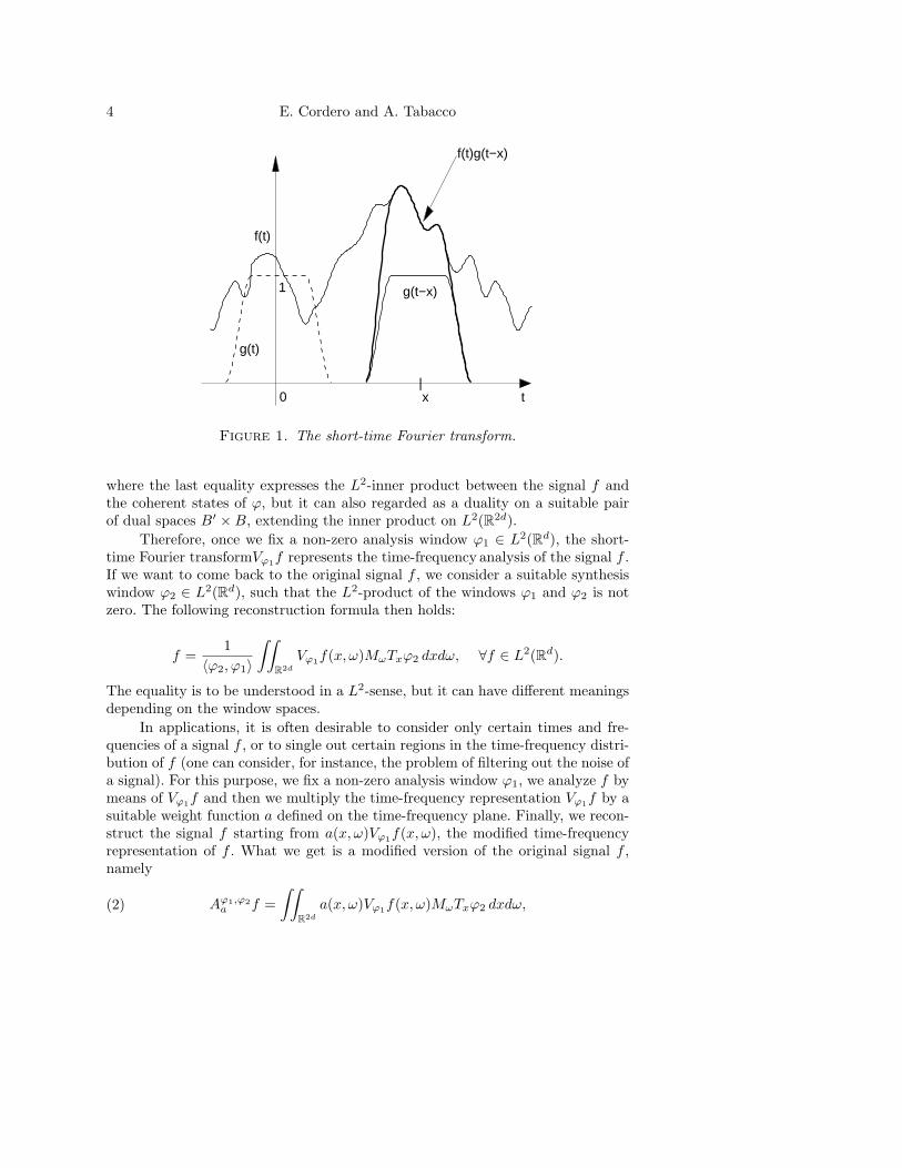
The localization operators can be defined by means of one of the most impor-tant and widely used time-frequency representation: the short-time Fourier trans-form, using once again the terminology of signal analysis. Why do we need a jointtime-frequency information about a signal? A simple example gives the answer toour question. For a given square integrable signal f , its Fourier transform f , the“spectrum” of f , is not sufficient to describe the physical phenomenon becauseit records which frequencies are present in the signal f , without saying anythingabout “when” those frequencies exist. The need to know how the spectral contentis changing in time, that is, to understand what a time-varying spectrum is, hasled to develop physical and mathematical ideas. Time-varying spectra are commonin ordinary life. The pitch, which is the common word for frequencies of humanspeech, changes as we speak and produces the richness of sounds in our language.The short time Fourier transform is the most widely used method for studyinga non-stationary signal, like human speech. The concept behind it is simple andpowerful. Suppose we listen to a piece of music that lasts an hour and supposethat it begins with violins and it ends with drums. If we Fourier analyze the wholehour by f , we see peaks at the frequencies corresponding to the violins and thedrums. This will tell us that there were violins and drums but will not give us anyindication of when the violins and drums were played. The most straightforwardway to overcome this lack of information is to break up the time interval intosmall segments (e.g., minutes) and Fourier analyze each interval resolutions. Thisis done by considering a suitable window function ϕ, localized in a neighborhoodof the origin (the initial time), and making it sliding along the time interval: thetime-frequency information about the signal f in a neighborhood of the instant xis obtained by Fourier-analyzing the product of f with the window ϕ shifted at x(see Figure 1).

This is the reason why we talk about short time Fourier transform. The short-time Fourier transform Vϕf of the signal f ∈ L2(Rd), with respect to the windowϕ ∈ L2(Rd), is given by

Vϕf(x, ω) =∫

Rd

f(t)ϕ(t− x) e−2πiωt dt = 〈f,MωTxϕ〉,


f(t)g(t−x)

f(t)

g(t)

g(t−x)1

0 x|

t

Figure 1. The short-time Fourier transform.

where the last equality expresses the L2-inner product between the signal f andthe coherent states of ϕ, but it can also regarded as a duality on a suitable pairof dual spaces B′ ×B, extending the inner product on L2(R2d).

Therefore, once we fix a non-zero analysis window ϕ1 ∈ L2(Rd), the short-time Fourier transformVϕ1f represents the time-frequency analysis of the signal f .If we want to come back to the original signal f , we consider a suitable synthesiswindow ϕ2 ∈ L2(Rd), such that the L2-product of the windows ϕ1 and ϕ2 is notzero. The following reconstruction formula then holds:

f =1

〈ϕ2, ϕ1〉∫∫

R2d

Vϕ1f(x, ω)MωTxϕ2 dxdω, ∀f ∈ L2(Rd).

The equality is to be understood in a L2-sense, but it can have different meaningsdepending on the window spaces.

In applications, it is often desirable to consider only certain times and fre-quencies of a signal f , or to single out certain regions in the time-frequency distri-bution of f (one can consider, for instance, the problem of filtering out the noise ofa signal). For this purpose, we fix a non-zero analysis window ϕ1, we analyze f bymeans of Vϕ1f and then we multiply the time-frequency representation Vϕ1f by asuitable weight function a defined on the time-frequency plane. Finally, we recon-struct the signal f starting from a(x, ω)Vϕ1f(x, ω), the modified time-frequencyrepresentation of f . What we get is a modified version of the original signal f ,namely

(2) Aϕ1,ϕ2a f =

∫∫

R2d

a(x, ω)Vϕ1f(x, ω)MωTxϕ2 dxdω,


where the meaning of the previous integrals depends on the spaces where we havechosen the symbol a and the windows ϕ1 and ϕ2. Informally, we have just definedthe time-frequency localization operator Aϕ1,ϕ2

a , associated with the symbol a andwith ϕ1 and ϕ2 as analysis and synthesis windows, respectively.

To prove regularity results for localization operators, it is often useful theweak definition of the previous integral, that is

〈Aϕ1,ϕ2a f, g〉 =

∫∫

R2d

a(x, ω) Vϕ1f(x, ω) 〈MωTxϕ2, g〉 dxdω(3)

= 〈a, Vϕ1f Vϕ2g〉 , for f, g ∈ S(Rd) .

The last equality shows that the action of a localization operator can be inter-preted as the action of its symbol on the pointwise product of two short-timeFourier transforms. The localization operator can be seen as a generalization ofthe anti-Wick construction, that is recaptured for ϕ1(t) = ϕ2(t) = 2d/4e−t2/2.The previous definition also extends Daubechies’ one, in which the analysis andsynthesis windows coincide. The time-frequency construction of a localization op-erator naturally suggests to replace the study of the linear anti-Wick quantizationmapping by the investigation of the multilinear mapping

(4) (a, ϕ1, ϕ2) 7→ Aϕ1,ϕ2a .

The result we get is a host of sufficient regularity conditions. Among the methodswe use to achieve the previous goal, there is the connection between anti-Wickoperator and Weyl calculus. To introduce Weyl operators, we use again a time fre-quency approach. Indeed we give a weak definition by means of another importanttime-frequency representation, the cross-Wigner distribution, defined as

W (f, g)(x, ω) =∫

Rd

e−2πiωtf(x +t

2)g(x− t

2) dt,

where f, g are suitable functions, chosen such as the previous integral makes sense.Given a symbol σ on the phase space R2d, the Weyl operator Lσ is defined as

(5) 〈Lσf, g〉 = 〈σ,W (g, f)〉, ∀f, g ∈ S(Rd).

The mapping

σ 7→ Lσ

is another quantization rule, and it is called Weyl quantization or Weyl transform[18, 32].

A localization operator can always be written as a Weyl operator. Namely, ifW (ϕ2, ϕ1) is the cross-Wigner distribution of ϕ2, ϕ1, and Lσ is the Weyl transformwith Weyl symbol σ, then we have (see [4, 18])

(6) Aϕ1,ϕ2a = La∗W (ϕ2,ϕ1).


3. Regularity results

In order to provide our result, we explicitly recall the definition of the functionspaces we will work with. Secondly, we present sufficient regularity results andfinally we show the (almost) optimality of the results obtained giving necessaryconditions.

3.1. Function spaces

If 1 ≤ p < ∞, then ‖f‖p =(∫Rd |f(x)|p dx

)1/p is the Lp-norm of f , and Lp(Rd), orjust Lp, is the Banach space of all measurable functions f that have finite Lp-norm.For p = ∞, L∞(Rd) is the space of essentially bounded measurable functions withthe norm ‖f‖∞ = ess supx∈Rd |f(x)|. In the next section we shall also make use ofthe weighted FLp-spaces. First, given a positive and continuous weight functionm on Rd, a function f belongs to the weighted Lp-spaces, i.e., f ∈ Lp

m(Rd) if andonly if the pointwise product fm is in ∈ Lp(Rd). Next, we define the FLp

m-spacesof functions as

FLpm(Rd) = {f ∈ S ′(Rd) : ∃ g ∈ Lp

m(Rd), g = f}.These spaces are Banach spaces equipped with the norm

‖f‖FLpm

= ‖g‖Lpm

, with g = f.

We now recall the definition of potential Sobolev spaces. Let s ∈ R, the Besselkernel is defined by

(7) Gs = F−1{(1 + | · |2)−s/2}.Then the potential Sobolev spaces are given by

(8) W ps = Gs ∗ Lp(Rd) = {f ∈ S ′, f = Gs ∗ g, g ∈ Lp},

with norm ‖f‖W ps

= ‖g‖p (see [3, 29]).The spaces that provide a measure of the phase space distribution of symbols

and windows, are the so-called modulation spaces. For their basic properties werefer, for instance, to [20, Ch. 11-13] and the original literature quoted there.

Firstly, let us introduce the weight functions we shall deal with. Let v be acontinuous, positive, even, submultiplicative weight function on R2d (in short, asubmultiplicative weight), i.e., v(0) = 1, v(z) = v(−z), and v(z1+z2) ≤ v(z1)v(z2),for all z, z1, z2 ∈ R2d. A positive, even weight function m on R2d is called v-moderate if m(z1 + z2) ≤ Cv(z1)m(z2) for all z1, z2 ∈ R2d. We shall mostly usethe previous weights when working with modulation spaces, even though we definethem for general weights.

Namely, let g ∈ S(Rd) be a fixed non-zero window, m a non-negative, evenweight function on R2d of polynomial growth, and 1 ≤ p, q ≤ ∞; the modulationspace Mp,q

m (Rd) consists of all tempered distributions f ∈ S ′(Rd) such that Vgf ∈


Lp,qm (R2d) (weighted mixed-norm spaces). The norm on Mp,q

m is

‖f‖Mp,qm

= ‖Vgf‖Lp,qm

=

(∫

Rd

(∫

Rd

|Vgf(x, ω)|pm(x, ω)p dx

)q/p

dω

)1/q

.

If p = q, we write Mpm instead of Mp,p

m , and if m(z) ≡ 1 on R2d, then we writeMp,q and Mp for Mp,q

m and Mp,pm , respectively.

Mp,qm (Rd) is a Banach space, whose definition is independent of the choice

of the window g ∈ S(Rd). Moreover, for any v-moderate weight m, and anynon-zero g ∈ S(Rd), then ‖Vgf‖Lp,q

mare equivalent norms for Mp,q

m (Rd) (see [20,Thm. 11.3.7]). In particular, we will use the polynomial weights defined by

vs(z) = vs(x, ω) = 〈z〉s = (1+x2 +ω2)s/2, τs(z) = τs(x, ω) = 〈ω〉s = (1+ω2)s/2,

where z = (x, ω) ∈ R2d and s ∈ R.Among the modulation spaces one can recognize well-known function spaces

(see [4, 22, 28]):(i) L2(Rd) = M2(Rd).(ii) Sobolev spaces: Hs(Rd) = {f : f(ω)〈ω〉s ∈ L2(Rd)} = M2

τs(Rd).

(iv) Shubin-Sobolev spaces:

(9) Qs(Rd) = L2s(Rd) ∩Hs(Rd) = M2

vs(Rd).

(v) Feichtinger’s algebra: M1(Rd) = S0(Rd).(vi) Schwartz class: S(Rd) =

⋂s≥0 M∞

vs(Rd) .

(vii) Space of tempered distributions: S ′(Rd) =⋃

s≥0 M∞1/vs

(Rd) .

For comparison we list the following embeddings between potential and mod-ulation spaces [6].

Lemma 3.1. For 1 ≤ p ≤ ∞ and s ∈ R, we have

W ps (Rd) ↪→ Mp,∞

τs(Rd).

3.2. Sufficient conditions

To present our result, we need to recall the definition of Schatten-von Neumannclasses. Consider a compact operator A ∈ B(X), where X is a separable Hilbertspace and B(X) is the space of bounded linear operators on X. For p ∈ [1,∞),the Schatten-von Neumann class is defined as

(10) Sp = {A ∈ B(X), with ‖A‖Sp :=∞∑

k=1

sk(A)p < ∞},

where sk(A) are the singular values of A, i.e., the eigenvalues of the operator√A∗A. In particular, S2 is the space of Hilbert-Schmidt operators, and S1 is the

space of trace class operators. For consistency, we define the class S∞ := B(X).Here we consider the Hilbert space X = L2(Rd). We write E ′(R2d) for the subspaceof tempered distributions of compact support on R2d.

The sufficient regularity conditions known so far can be easily summarizedby means of the following table.


Results Symbol Windows Operatora ϕ1 ϕ2 Aϕ1,ϕ2

a

(i) Lp(R2d) L2(Rd) L2(Rd) Sp

(ii) W p−s(R2d), s > 0 M1

vs(Rd) M1

vs(Rd) Sp

(iii) M∞1/τs

(R2d) M1vs

(Rd) M1vs

(Rd) B(Mp,q(Rd))(iv) H−s(R2d), M2

vs(Rd) M2

vs(Rd) S2

(v) Mp,∞1/τs

(R2d), M1vs

(Rd) M1vs

(Rd) Sp

(vi) E ′(R2d) S(Rd) S(Rd) S1

The result (i) is well known and first appeared in [34]; here we sketch adifferent and shorter proof of it. More details are contained in [4].

Theorem 3.2. If ϕ1, ϕ2 ∈ L2(Rd) and a ∈ Lp(R2d) for 1 ≤ p ≤ ∞, then Aϕ1,ϕ2a ∈

Sp and

(11) ‖Aϕ1,ϕ2a ‖Sp

≤ ‖a‖p ‖ϕ1‖2 ‖ϕ2‖2 .

Proof. We prove the result for trace class p = 1 and the boundedness for p = ∞and then interpolate between these endpoints.

(a) p = 1.For z = (x, ω) ∈ R2d, we consider the rank one operator

Qzf = 〈f,MωTxϕ1〉MωTxϕ2.

Its trace class norm is‖Qz‖S1 = ‖ϕ1‖2 ‖ϕ2‖2

and the mapping z 7→ Qz is continuous from R2d to S1. Therefore the vector-valuedintegral defining Aϕ1,ϕ2

a as

Aϕ1,ϕ2a =

∫∫

R2d

a(z)Qz dz

is well-defined in S1 (see, e.g., [25]). The generalized triangle inequality now yields

‖Aϕ1,ϕ2a ‖S1 ≤

∫∫

R2d

|a(z)| ‖Qz‖S1 dz = ‖a‖1 ‖ϕ1‖2 ‖ϕ2‖2.

(b) p = ∞.In this case we use the weak definition (3) of Aϕ1,ϕ2

a and estimate directly

|〈Aϕ1,ϕ2a f, g〉| = |〈a, Vϕ1f Vϕ2g〉| ≤ ‖a‖∞ ‖Vϕ1f Vϕ2g‖1

≤ ‖a‖∞ ‖Vϕ1f‖2 ‖Vϕ2g‖2 = ‖a‖∞ ‖ϕ1‖2 ‖ϕ2‖2 ‖f‖2 ‖g‖2 .

In the last equality we used the isometry property of the short-time Fourier trans-form [20, Chp.3], given by

‖Vϕf‖L2(R2d) = ‖f‖L2(Rd)‖ϕ‖L2(Rd) f, ϕ ∈ L2(Rd).

It follows that Aϕ1,ϕ2a is bounded on L2(Rd) and (11) holds for p = ∞.

The result follows now by complex interpolation.


The results (ii) − (vi) were proved by a different method. Namely, thanks torelation (6), finding sufficient regularity conditions for localization operators canbe translated into seeking conditions for Weyl operators. In this last framework,there are many papers and results on the topic. The most recent and general onesinvolve modulation spaces (see [6, 21]) and can be summarized as follows.

Theorem 3.3. (i) If σ ∈ M∞,1(R2d), then Lσ is bounded on Mp,q(Rd), where1 ≤ p, q ≤ ∞, with a uniform estimate ‖Lσ‖op <∼ ‖σ‖M∞,1 for the operator norm.In particular, Lσ is bounded on L2(Rd).

(ii) If σ ∈ M1(R2d), then Lσ ∈ S1 and ‖Lσ‖S1 <∼ ‖σ‖M1 .(iii) If 1 ≤ p ≤ 2 and σ ∈ Mp(R2d), then Lσ ∈ Sp and ‖Lσ‖Sp

<∼ ‖σ‖Mp .

(iv) If 2 ≤ p ≤ ∞ and σ ∈ Mp,p′(R2d), then Lσ ∈ Sp and ‖Lσ‖Sp<∼ ‖σ‖Mp,p′ .

Relation (6) provides the (Weyl) symbol of Aϕ1,ϕ2a , that is

(12) σ = a ∗W (ϕ2, ϕ1) .

Therefore, if we want to use Theorem 3.3, we need to understand convolutionrelations between modulation spaces and properties of the Wigner distribution.This is made clear by the following two propositions, proved in [6]. Let us noticethat the first result shows a convolution relation for modulation spaces in the styleof Young’s theorem.

Proposition 3.4. Let v be a submultiplicative weight on R2d and m be a v-moderateweight. We write m1(x) = m(x, 0) and m2(ω) = m(0, ω) for the restrictions toRd × {0} and {0} × Rd, and likewise for v. Let ν(ω) > 0 be an arbitrary weightfunction on Rd and 1 ≤ p, q, r, s, t ≤ ∞. If

1p

+1q− 1 =

1r, and

1t

+1t′

= 1 ,

then

(13) Mp,stm1⊗ν(Rd) ∗Mq,st′

v1⊗v2ν−1(Rd) ↪→ Mr,sm (Rd)

with norm inequality ‖f ∗ h‖Mr,sm

<∼ ‖f‖Mp,stm1⊗ν

‖h‖Mq,st′

v1⊗v2ν−1.

Next, the modulation space norm of a cross-Wigner distribution is controlledby means of the modulation space norms of the corresponding windows.

Proposition 3.5. If 1 ≤ p ≤ ∞, s ≥ 0, ϕ1 ∈ M1vs

(Rd) and ϕ2 ∈ Mpvs

(Rd), thenW (ϕ2, ϕ1) ∈ M1,p

τs(R2d), and

(14) ‖W (ϕ2, ϕ1)‖M1,pτs

<∼ ‖ϕ1‖M1vs‖ϕ2‖Mp

vs.

Based on the tools developed so far, it is now straightforward to prove thesufficient regularity conditions for localization operators contained in the followingtheorem (for details we refer to [6]).


Theorem 3.6. (i) Let s ≥ 0. If 1 ≤ p ≤ 2, then the mapping (a, ϕ1, ϕ2) 7→ Aϕ1,ϕ2a

is bounded from Mp,∞1/τs

(R2d)×M1vs

(Rd)×Mpvs

(Rd) into Sp; in other words,

‖Aϕ1,ϕ2a ‖Sp

<∼ ‖a‖Mp,∞1/τs

‖ϕ1‖M1vs‖ϕ2‖Mp

vs.

(ii) If 2 ≤ p ≤ ∞, then the mapping (a, ϕ1, ϕ2) 7→ Aϕ1,ϕ2a is bounded from Mp,∞

1/τs×

M1vs×Mp′

vsinto Sp, and

‖Aϕ1,ϕ2a ‖Sp

<∼ ‖a‖Mp,∞1/τs

‖ϕ1‖M1vs‖ϕ2‖Mp′

vs

.

(iii) If a ∈ M∞1/τs

(R2d), ϕ1, ϕ2 ∈ M1vs

(Rd), then Aϕ1,ϕ2a is bounded on Mp,q(Rd)

for all 1 ≤ p, q ≤ ∞, and the operator norm satisfies the uniform estimate

‖Aϕ1,ϕ2a ‖op <∼ ‖a‖M∞

1/τs‖ϕ1‖M1

vs‖ϕ2‖M1

vs.

Using the embedding result of Lemma 3.1 and the embedding M1vs

↪→ Mpvs

,with 1 ≤ p ≤ ∞ (see e.g., [20]), we derive the result (ii):

Corollary 3.7. Let a ∈ W p−s(R2d) for some s ≥ 0, 1 ≤ p ≤ ∞, and ϕ1, ϕ2 ∈

M1vs

(Rd). Then

‖Aϕ1,ϕ2a ‖Sp

<∼ ‖a‖W p−s‖ϕ1‖M1

vs‖ϕ2‖M1

vs.

Let us end up this subsection saying few words about tempered distributi-ons of compact support E ′(R2d). It is well-known that every a ∈ E ′(R2d) can berepresented as

(15) a =∑

|α|≤n

∂αfα

for compactly supported continuous functions fα on R2d [31, p. 263, Cor. 2]. Forconvenience and in contrast to the standard definition, we will call the integer nin (15) the order of a ∈ E ′. If we compute the short-time Fourier transform of atempered distribution of order n, we get the estimate (see [6, Prop. 3.6])

|Vga(x, ω)| ≤ CN 〈x〉−N 〈ω〉n ∀N ∈ N ,

and, consequently, a ∈ M1,∞1/τn

(Rd). If ϕ1, ϕ2 ∈ M1vn

(Rd), then Theorem 3.6(i)implies that Aϕ1,ϕ2

a is a trace class operator.

3.3. Necessary conditions

In this section we show that the sufficient conditions obtained in Theorem 3.6 (forp = ∞ and p = 2) are essentially optimal. This investigation requires a differentapproach. The starting point is a local regularity property of the short-time Fouriertransform, written in terms of Wiener amalgam spaces [14, 15, 17, 19]. Here we donot intend to come into this matter. Moreover, the proof of the necessary conditionsis achieved by heavily working with short-time Fourier transform properties and itrequires a broad background on the topic. Therefore, we limit ourselves to presentthe result, referring the reader to [6], for all the proofs and details.


Theorem 3.8. Let a ∈ S ′(R2d) and s ≥ 0.(i) If there exists a constant C = C(a) > 0, depending only on a, such that

(16) ‖Aϕ1,ϕ2a ‖S∞ ≤ C ‖ϕ1‖M1

vs‖ϕ2‖M1

vs

for all ϕ1, ϕ2 ∈ S(Rd), then a ∈ M∞1/τs

.(ii) If there exists a constant C = C(a) > 0, depending only on a, such that

(17) ‖Aϕ1,ϕ2a ‖S2 ≤ C ‖ϕ1‖M1‖ϕ2‖M1

for all ϕ1, ϕ2 ∈ S(Rd), then a ∈ M2,∞.

Let us end up this section by giving an application of localization operatorswith rough symbols. Namely, symbols that are tempered distributions enable us towork with bounded measures of the form a =

∑k∈Z2d akδk, where (ak) ∈ `∞ (the

space of bounded sequences) and δk is the Dirac measure centered at the pointk. If we substitute the previous measure to the function a in the definition (2)of a localization operator, we recapture the discrete Gabor multiplier [16], with aconsiderable improvement of the regularity results known so far.

4. Composition formula

Given two localization operators, we aim at computing their product. It would beuseful to express it in terms of localization operators. In the sequel we present twodifferent product formulae. The former is an exact formula, i.e., the compositionresult is a localization operator as well. However, the formula holds only for Gauss-ian windows. The latter works for every pair of localization operators; in this case,the result is written as a sum of localization operators, plus a remainder term, inthe Weyl form.

4.1. Exact product

We reformulate the result of [13] according to the notation of [18, 20]. Furthermore,we provide regularity estimates in dependence of the function spaces the symbolsof the factors belong to.

From then onward we consider the window functions ϕ1(t) = ϕ2(t) = ϕ(t) =2d/4e−πt2 , t ∈ Rd. In this case, the Wigner distribution of the Gaussian ϕ is aGaussian as well: W (ϕ,ϕ)(z) = 2d/2e−2πz2

, z ∈ R2d. If we compute the Weylsymbol σ of the operator Aϕ,ϕ

a , by means of relation (6) we get σ(ζ) = 2d/2(a ∗e−2πz2

)(ζ), z, ζ ∈ R2d. In order to express the product in the localization form,firstly, we rewrite the factors in a Weyl form and then we use the product formulafor Weyl operators [18, Chp. 3.2]. Namely, the composition of the Weyl operatorsLσ and Lτ , with symbols σ and τ belonging to suitable function spaces, is a Weyloperator Lµ, with symbol µ = σ]τ , the twisted multiplication of the symbols σand τ :

σ]τ(ζ) = 22d

∫∫

R2d

σ(z)τ(w)e4πi[ζ−w,ζ−z] dzdw,


where the brackets [·, ·] express the symplectic form on R2d, i.e.,

[(z1, z2), (ζ1, ζ2)] = z1ζ2 − z2ζ1, with z = (z1, z2), ζ = (ζ1, ζ2).

Secondly, we come back to localization operators by means of relation (6). Giventhe Weyl symbols σ, τ ∈ S(R2d), we are interested in the Fourier transform of thetwisted multiplication σ]τ , that is

F(σ]τ)(ζ) = σ\τ(ζ),

where the twisted product \ is given by

(18) σ\τ(ζ) =∫∫

R2d

σ(z)τ(ζ − z)eπi[z,ζ] dz.

For any f, g ∈ S(R2d), we define the \[ product by

(19) f\[g(ζ) =∫∫

R2d

f(z)g(z − ζ)eπ(zζ+i[z,ζ]) dz,

then the product of localization operators is given by the following result.

Theorem 4.1. Let a, b ∈ S(R2d). If there exists a symbol c ∈ S ′(R2d) so that

(20) c = 2−d/2a\[b,

then we haveAϕ,ϕ

a Aϕ,ϕb = Aϕ,ϕ

c .

Proof. It is a straightforward consequence of relations (18) and (19). Indeed, werewrite Aϕ,ϕ

a Aϕ,ϕb in the Weyl form and we use relation (18) for the Weyl product:

the result is the Weyl operator Lµ, where the Fourier transform of µ is given by

µ(ζ) = F(a ∗W (ϕ,ϕ))\F(b ∗W (ϕ,ϕ))

= 2−d

∫∫

R2d

a(z)b(z − ζ)e−(π/2)z2e−(π/2)(ζ−z)2eπi[z,ζ] dz

= 2−de−(π/2)ζ2∫∫

R2d

a(z)b(z − ζ)eπ(zζ+i[z,ζ]) dz.

Hence, we have

µ(ζ) = c(ζ)(2−d/2e−(π/2)ζ2) = F(c ∗W (ϕ, ϕ))(ζ),

where c is given by relation (20).

Next, we want to obtain estimates related to the product \[.

Lemma 4.2. Let f, g ∈ S(R2d) and h = f\[g. Then, for every constant δ > 0, wehave

(21) |h(ζ)| <∼(|f(z)|e(π/2)(2+δ2)z2 ∗ |g(z)|e(π/2δ2)z2)

(ζ), ∀ζ ∈ R2d.


Proof. We have

eπzζ ≤ eπ|z| |ζ| ≤ eπz2 |ζ−z| |z| = eπz2eπ|ζ−z|2/2δ2

eπδ2|z|2/2

≤ eπ(2+δ2)(z2/2)eπ|ζ−z|2/2δ2,

then the result is obtained using relation (19).

Theorem 4.3. Let δ > 0 be fixed. If a ∈ FLp

e(π/2)(2+δ2)z2 (R2d), b ∈ FLq

e(π/2δ2)z2 (R2d),with 1 ≤ p, q ≤ ∞, then the product Aϕ,ϕ

a Aϕ,ϕb = Aϕ,ϕ

c gives a localization operatorAϕ,ϕ

c with symbol c satisfying

(22) c ∈ FLr(R2d), with1r

=1p

+1q− 1.

Proof. It is a straightforward consequence of Young inequality applied to relation(21).

Corollary 4.4. Consider the symbols a ∈ FLp

e(π/2)(2+δ2)z2 (R2d), b ∈ FLq

e(π/2δ2)z2 (R2d),with

1p

+1q

=32,

then the product Aϕ,ϕa Aϕ,ϕ

b = Aϕ,ϕc gives an Hilbert-Schmidt localization operator.

Proof. Using Theorem 4.3, we get c ∈ FL2. Therefore c ∈ L2 and the correspond-ing localization operator Aϕ,ϕ

c is a Hilbert-Schmidt operator (see [6]).

Let us observe that, using the same technique as in Corollary 4.4, one canalso obtain Schatten-class property for the product of two localization operators.

4.2. Asymptotic product

We end up this section by giving some hints about an asymptotic formula for theproduct. The motivation comes up from the previous subsection: the product oftwo localization operators with symbols belonging to some classes does not yield,in general, to a localization operator with symbol in the same class.

In the framework of PDE, the product of two localization operators has beenwritten as a sum of localization operators plus a remainder term expressed ina Weyl, instead of a localization operator, form. The localization operators ofthis sum have symbols given by pointwise multiplications of the first symbol withderivatives of the second one, while the windows are the same as the factors,but only for Gaussian windows [1]. For the most general formula in the classicalframework we refer to [7, 8]; the extension to modulation spaces is contained in [5]and is presented in the subsequent relation (23). In the PDE context, the operatorsymbols belong to smooth classes, such as the Shubin or the Hormander classes[23, 28]. In the previous works it has been shown that the bigger the derivativeorder, the more regular the symbol is. Moreover, the Weyl symbol of the remainderterm belongs to a class more regular than the localization symbol of the sum, sothat the Weyl remainder could be omitted.


Our point of view is signal analysis rather than PDE. In this context, wedeal with rougher symbols and windows, even tempered distributions rather thanfunctions are allowed; the symbol classes do not enjoy the property of increasingregularity with the derivative order , typical of the classical case. Hence, the Weylremainder symbol might be less regular than the localization symbols containedin the sum. It is clear that a different approach is required. The interest is focusedon norm estimates for the operators. Since it is hopeless to find a more regularsymbol for the remainder when rough symbols are considered, it is fundamen-tal to understand when the localization operators and the Weyl remainder arebounded on suitable Banach spaces. Furthermore, for some applications (e.g., thecharacterization given by (24)), the Weyl term compactness is needed.

This approach allows to measure how much a localization operator affectsthe time-frequency concentration of a signal. As usual, the spaces that give time-frequency measures are the modulation spaces. How do we translate the classicalproduct formula [1, 7, 8] in this context? How much can we extend it to hold forrough symbols and windows? How can pointwise symbol multiplication be madewhen it comes to tempered distributions?

The starting point is the product formula for localization operators containedin [8]. We translate the Shubin calculus into a corresponding one for symbols inmodulation spaces. Let us sketch the main results obtained in [5].

Let N ∈ N be fixed and ϕi, i = 1, . . . , 4, be non-zero windows in S(Rd) (evenrougher windows are allowed, with smoothness depending on the integer N). Ifwe consider any rough symbol a ∈ ⋃

s≥0 M∞1/vs

(R2d) = S ′(Rd) and we choose asymbol b smooth enough to make the pointwise multiplication ab ∈ M∞

1/τs(R2d)

(e.g., b lives in suitable Wiener amalgam spaces), then the composition of the twooperators Aϕ1,ϕ2

a and Aϕ3,ϕ4b can be written as

(23) Aϕ1,ϕ2a Aϕ3,ϕ4

b =N−1∑

|α|=0

(−1)|α|

α!AΦα,ϕ2

a∂αb + Lσ.

Namely, the product is expressed in terms of a sum of localization operators havingthe first window Φα made of the factor windows ϕ1, ϕ3, ϕ4 and depending on thederivative order (for the detailed expression we refer to [5, 8]); the remainder Lσ

is a Weyl operator. Moreover, one hasFormula (23) is well-defined on every modulation space Mp,q; i.e., the op-

erators on the right hand-side are all linear and bounded on every Mp,q.

Also operator norm estimates, involving the time-frequency distribution ofsymbols and windows can be easily provided. Here we end up recalling an im-portant application of formula (23). Indeed, formula (23) enables us to get a nicecharacterization of the weighted modulation space Mp,q

m (Rd), where m is a v-moderate weight. Indeed, if we write the composition formula (23) in the caseN = 1 and b = 1/a, where a ∈ C1(R2d) is a positive weight function satisfying thefollowing properties:


(i) a(z) ³ m(z);(ii) for j = 1, . . . , 2d, we have

(∂ja)(z)v(z)m2(z)

→ 0 for |z| → ∞,

then, the weighted modulations spaces Mp,qm can be defined as localization operator

pre-images of the un-weighted Mp,q. In details, in [5, Thm.7.3], we get the followingcharacterization for weighted modulation spaces:

(24) Mp,qm (Rd) = (Aϕ,ϕ

a )−1Mp,q(Rd),

for any non-zero window ϕ ∈ S(Rd). Relation (24) represents a generalization ofthe classical result for Shubin-Sobolev spaces [28], recaptured in the framework ofmodulation spaces by means of (9).

References

[1] H. Ando and Y. Morimoto. Wick calculus and the Cauthy problem for some dispersiveequations. Osaka J. Math., 39(1):123–147, 2002.

[2] F. A. Berezin. Wick and anti-Wick symbols of operators. Mat. Sb. (N.S.), 86(128):578–610, 1971.

[3] J. Bergh and J. Lofstrom. Interpolation spaces. An introduction. Springer-Verlag,Berlin, 1976.

[4] P. Boggiatto, E. Cordero, and K. Grochenig. Generalized Anti-Wick operators withsymbols in distributional Sobolev spaces. Integral Equations and Operator Theory, toappear.

[5] E. Cordero and K. Grochenig. Symbolic calculus for localization operators in modu-lation spaces. Preprint, 2003.

[6] E. Cordero and K. Grochenig. Time-frequency analysis of Localization operators. J.Funct. Anal., 205(1):107–131, 2003.

[7] E. Cordero, F. Nicola, and L. Rodino. Microlocal Analysis and applications to PDE.In Advances in Pseudo-Differential Operators, Operator Theory: Advances and Ap-plications (4th ISAAC Congress, 2003). Birkhauser.

[8] E. Cordero and L. Rodino. Wick calculus: a time-frequency approach. Osaka Journalof Mathematics, to appear.

[9] A. Cordoba and C. Fefferman. Wave packets and Fourier integral operators. Comm.Partial Differential Equations, 3(11):979–1005, 1978.

[10] I. Daubechies. Time-frequency localization operators: a geometric phase space ap-proach. IEEE Trans. Inform. Theory, 34(4):605–612, 1988.

[11] F. De Mari, H. G. Feichtinger, and K. Nowak. Uniform eigenvalue estimates for time-frequency localization operators. J. London Math. Soc. (2), 65(3):720–732, 2002.

[12] F. De Mari and K. Nowak. Localization type Berezin-Toeplitz operators on boundedsymmetric domains. J. Geom. Anal., 12(1):9–27, 2002.

[13] J. Du and M. W. Wong. A product formula for localization operators. Bull. KoreanMath. Soc., 37(1):77–84, 2000.


[14] H. G. Feichtinger. Banach convolution algebras of Wiener type. In Functions, series,operators, Vol. I, II (Budapest, 1980), pages 509–524. North-Holland, Amsterdam,1983.

[15] H. G. Feichtinger. Generalized amalgams, with applications to Fourier transform.Canad. J. Math., 42(3):395–409, 1990.

[16] H. G. Feichtinger and K. Nowak. A first survey of Gabor multipliers. In Advancesin Gabor analysis, Appl. Numer. Harmon. Anal., pages 99–128. Birkhauser Boston,Boston, MA, 2003.

[17] H. G. Feichtinger and G. Zimmermann. A Banach space of test functions for Gaboranalysis. In Gabor analysis and algorithms, pages 123–170. Birkhauser Boston, Boston,MA, 1998.

[18] G. B. Folland. Harmonic analysis in phase space. Princeton Univ. Press, Princeton,NJ, 1989.

[19] J. J. F. Fournier and J. Stewart. Amalgams of Lp and lq. Bull. Amer. Math. Soc.(N.S.), 13(1):1–21, 1985.

[20] K. Grochenig. Foundations of Time-Frequency Analysis. Birkhauser, Boston, 2001.

[21] K. Grochenig and C. Heil. Modulation spaces and pseudodifferential operators. In-tegral Equations Operator Theory, 34(4):439–457, 1999.

[22] K. Grochenig and G. Zimmermann. Hardy’s theorem and the short-time Fouriertransform of Schwartz functions. J. London Math. Soc., 63:205–214, 2001.

[23] L. Hormander. The analysis of linear partial differential operators. III, volume 274 ofGrundlehren der Mathematischen Wissenschaften [Fundamental Principles of Math-ematical Sciences]. Springer-Verlag, Berlin, 1994.

[24] R. Howe. Quantum mechanics and partial differential equations. J. Funct. Anal.,38(2):188–254, 1980.

[25] Y. Katznelson. An introduction to harmonic analysis. John Wiley & Sons, New York,1968.

[26] N. Lerner. The Wick calculus of pseudo-differential operators and energy estimates.In New trends in microlocal analysis (Tokyo, 1995), pages 23–37. Springer, Tokyo,1997.

[27] J. Ramanathan and P. Topiwala. Time-frequency localization via the Weyl corre-spondence. SIAM J. Math. Anal., 24(5):1378–1393, 1993.

[28] M. A. Shubin. Pseudodifferential operators and spectral theory. Springer-Verlag,Berlin, second edition, 2001.

[29] E. M. Stein. Singular integrals and differentiability properties of functions. PrincetonUniv. Press, Princeton, NJ, 1970.

[30] J. Toft. Continuity properties for modulation spaces with applications in pseudo-differential calculus, I. J. Funct. Anal., to appear.

[31] F. Treves. Topological vector spaces, distributions and kernels. Academic Press, NewYork, 1967.

[32] M. W. Wong. Weyl transforms. Springer-Verlag, New York, 1998.

[33] M. W. Wong. Localization operators. Seoul National University Research Instituteof Mathematics Global Analysis Research Center, Seoul, 1999.


[34] M. W. Wong. Wavelet transforms and localization operators, volume 136 of OperatorTheory: Advances and Applications. Birkhauser Verlag, Basel, 2002.

Department of Mathematics, Politecnico of Torino, Corso Duca degli Abruzzi 24,10129 Torino, ItalyE-mail address: [email protected], [email protected] address: [email protected]

Localization Operators Via Time-Frequency Analysis

Documents

Transcript of Localization Operators Via Time-Frequency Analysis