
Robust Control Toolbox User's Guide
182
Robust Control Toolbox™ User's Guide Gary Balas Richard Chiang Andy Packard Michael Safonov R2015b
-
Upload
khangminh22 -
Category
Documents
-
view
1 -
download
0
Transcript of Robust Control Toolbox User's Guide

Robust Control Toolbox™
User's Guide
Gary BalasRichard ChiangAndy PackardMichael Safonov
R2015b
How to Contact MathWorks
Latest news: www.mathworks.com
Sales and services: www.mathworks.com/sales_and_services
User community: www.mathworks.com/matlabcentral
Technical support: www.mathworks.com/support/contact_us
Phone: 508-647-7000
The MathWorks, Inc.3 Apple Hill DriveNatick, MA 01760-2098
Robust Control Toolbox™ User's Guide© COPYRIGHT 2005–2015 by The MathWorks, Inc.The software described in this document is furnished under a license agreement. The software may be usedor copied only under the terms of the license agreement. No part of this manual may be photocopied orreproduced in any form without prior written consent from The MathWorks, Inc.FEDERAL ACQUISITION: This provision applies to all acquisitions of the Program and Documentationby, for, or through the federal government of the United States. By accepting delivery of the Programor Documentation, the government hereby agrees that this software or documentation qualifies ascommercial computer software or commercial computer software documentation as such terms are usedor defined in FAR 12.212, DFARS Part 227.72, and DFARS 252.227-7014. Accordingly, the terms andconditions of this Agreement and only those rights specified in this Agreement, shall pertain to andgovern the use, modification, reproduction, release, performance, display, and disclosure of the Programand Documentation by the federal government (or other entity acquiring for or through the federalgovernment) and shall supersede any conflicting contractual terms or conditions. If this License failsto meet the government's needs or is inconsistent in any respect with federal procurement law, thegovernment agrees to return the Program and Documentation, unused, to The MathWorks, Inc.
Trademarks
MATLAB and Simulink are registered trademarks of The MathWorks, Inc. Seewww.mathworks.com/trademarks for a list of additional trademarks. Other product or brandnames may be trademarks or registered trademarks of their respective holders.Patents
MathWorks products are protected by one or more U.S. patents. Please seewww.mathworks.com/patents for more information.

Revision History
September 2005 First printing New for Version 3.0.2 (Release 14SP3)March 2006 Online only Revised for Version 3.1 (Release 2006a)September 2006 Online only Revised for Version 3.1.1 (Release 2006b)March 2007 Online only Revised for Version 3.2 (Release 2007a)September 2007 Online only Revised for Version 3.3 (Release 2007b)March 2008 Online only Revised for Version 3.3.1 (Release 2008a)October 2008 Online only Revised for Version 3.3.2 (Release 2008b)March 2009 Online only Revised for Version 3.3.3 (Release 2009a)September 2009 Online only Revised for Version 3.4 (Release 2009b)March 2010 Online only Revised for Version 3.4.1 (Release 2010a)September 2010 Online only Revised for Version 3.5 (Release 2010b)April 2011 Online only Revised for Version 3.6 (Release 2011a)September 2011 Online only Revised for Version 4.0 (Release 2011b)March 2012 Online only Revised for Version 4.1 (Release 2012a)September 2012 Online only Revised for Version 4.2 (Release 2012b)March 2013 Online only Revised for Version 4.3 (Release 2013a)September 2013 Online only Revised for Version 5.0 (Release 2013b)March 2014 Online only Revised for Version 5.1 (Release 2014a)October 2014 Online only Revised for Version 5.2 (Release 2014b)March 2015 Online only Revised for Version 5.3 (Release 2015a)September 2015 Online only Revised for Version 6.0 (Release 2015b)

v
Contents
Building Uncertain Models1
Introduction to Uncertain Elements . . . . . . . . . . . . . . . . . . . . 1-3
Uncertain Real Parameters . . . . . . . . . . . . . . . . . . . . . . . . . . . 1-5
Create Uncertain Real Parameters . . . . . . . . . . . . . . . . . . . . . 1-7
Uncertain LTI Dynamics Elements . . . . . . . . . . . . . . . . . . . . 1-14Time Domain of ultidyn Elements . . . . . . . . . . . . . . . . . . . . 1-15
Create Uncertain LTI Dynamics . . . . . . . . . . . . . . . . . . . . . . 1-17
Uncertain Complex Parameters and Matrices . . . . . . . . . . . 1-18Uncertain Complex Parameters . . . . . . . . . . . . . . . . . . . . . 1-18Uncertain Complex Matrices . . . . . . . . . . . . . . . . . . . . . . . . 1-19
Systems with Unmodeled Dynamics . . . . . . . . . . . . . . . . . . . 1-22
Uncertain Matrices . . . . . . . . . . . . . . . . . . . . . . . . . . . . . . . . . 1-23
Create Uncertain Matrices from Uncertain Elements . . . . . 1-24
Access Properties of a umat . . . . . . . . . . . . . . . . . . . . . . . . . . 1-25
Row and Column Referencing . . . . . . . . . . . . . . . . . . . . . . . . 1-27
Matrix Operation on umat Objects . . . . . . . . . . . . . . . . . . . . 1-29
Evaluate Uncertain Elements by Substitution . . . . . . . . . . . 1-31Lifting a double matrix to a umat . . . . . . . . . . . . . . . . . . . . 1-32
vi Contents
Uncertain State-Space Models (uss) . . . . . . . . . . . . . . . . . . . 1-33Properties of uss Objects . . . . . . . . . . . . . . . . . . . . . . . . . . . 1-33
Create Uncertain State-Space Model . . . . . . . . . . . . . . . . . . 1-36
Sample Uncertain Systems . . . . . . . . . . . . . . . . . . . . . . . . . . . 1-37
Feedback Around an Uncertain Plant . . . . . . . . . . . . . . . . . 1-39
Interpreting Uncertainty in Discrete Time . . . . . . . . . . . . . 1-41
Lifting a ss to a uss . . . . . . . . . . . . . . . . . . . . . . . . . . . . . . . . . 1-42
Create Uncertain Frequency Response Data Models . . . . . 1-43Properties of ufrd Objects . . . . . . . . . . . . . . . . . . . . . . . . . . 1-44
Interpreting Uncertainty in Discrete Time . . . . . . . . . . . . . 1-46
Lifting an frd to a ufrd . . . . . . . . . . . . . . . . . . . . . . . . . . . . . . 1-47
Basic Control System Toolbox and MATLABInterconnections . . . . . . . . . . . . . . . . . . . . . . . . . . . . . . . . . 1-48
Simplifying Representation of Uncertain Objects . . . . . . . . 1-49Effect of the Autosimplify Property . . . . . . . . . . . . . . . . . . . 1-50Direct Use of simplify . . . . . . . . . . . . . . . . . . . . . . . . . . . . . 1-52
Generate Samples of Uncertain Systems . . . . . . . . . . . . . . . 1-53Generating One Sample . . . . . . . . . . . . . . . . . . . . . . . . . . . 1-53Generating Many Samples . . . . . . . . . . . . . . . . . . . . . . . . . 1-53Sampling ultidyn Elements . . . . . . . . . . . . . . . . . . . . . . . . . 1-54
Substitution by usubs . . . . . . . . . . . . . . . . . . . . . . . . . . . . . . . 1-57Specifying the Substitution with Structures . . . . . . . . . . . . 1-58Nominal and Random Values . . . . . . . . . . . . . . . . . . . . . . . 1-58
Array Management for Uncertain Objects . . . . . . . . . . . . . . 1-60
Reference Into Arrays . . . . . . . . . . . . . . . . . . . . . . . . . . . . . . . 1-61
Create Arrays with stack and cat Functions . . . . . . . . . . . . 1-62
Create Arrays by Assignment . . . . . . . . . . . . . . . . . . . . . . . . 1-64

vii
Binary Operations with Arrays . . . . . . . . . . . . . . . . . . . . . . . 1-65
Create Arrays with usample . . . . . . . . . . . . . . . . . . . . . . . . . 1-66
Create Arrays with usubs . . . . . . . . . . . . . . . . . . . . . . . . . . . . 1-68
Create Arrays with gridureal . . . . . . . . . . . . . . . . . . . . . . . . . 1-69
Create Arrays with repmat . . . . . . . . . . . . . . . . . . . . . . . . . . 1-70
Create Arrays with repsys . . . . . . . . . . . . . . . . . . . . . . . . . . . 1-71
Using permute and ipermute . . . . . . . . . . . . . . . . . . . . . . . . . 1-72
Decomposing Uncertain Objects . . . . . . . . . . . . . . . . . . . . . . 1-73Normalizing Functions for Uncertain Elements . . . . . . . . . . 1-73Properties of the Decomposition . . . . . . . . . . . . . . . . . . . . . 1-74Syntax of lftdata . . . . . . . . . . . . . . . . . . . . . . . . . . . . . . . . . 1-75Advanced Syntax of lftdata . . . . . . . . . . . . . . . . . . . . . . . . . 1-77
Generalized Robustness Analysis2
Generalized Robustness Analysis . . . . . . . . . . . . . . . . . . . . . . 2-2
Robust Stability Margin . . . . . . . . . . . . . . . . . . . . . . . . . . . . . . 2-4
Robust Performance Margin . . . . . . . . . . . . . . . . . . . . . . . . . . 2-5
Worst-Case Gain Measure . . . . . . . . . . . . . . . . . . . . . . . . . . . . . 2-6
Introduction to Linear Matrix Inequalities3
Linear Matrix Inequalities . . . . . . . . . . . . . . . . . . . . . . . . . . . . 3-2LMI Features . . . . . . . . . . . . . . . . . . . . . . . . . . . . . . . . . . . . 3-2
viii Contents
LMIs and LMI Problems . . . . . . . . . . . . . . . . . . . . . . . . . . . . . . 3-4
LMI Applications . . . . . . . . . . . . . . . . . . . . . . . . . . . . . . . . . . . . 3-6Stability . . . . . . . . . . . . . . . . . . . . . . . . . . . . . . . . . . . . . . . . 3-7RMS Gain . . . . . . . . . . . . . . . . . . . . . . . . . . . . . . . . . . . . . . . 3-8LQG Performance . . . . . . . . . . . . . . . . . . . . . . . . . . . . . . . . . 3-8
Further Mathematical Background . . . . . . . . . . . . . . . . . . . . 3-10
Bibliography . . . . . . . . . . . . . . . . . . . . . . . . . . . . . . . . . . . . . . . 3-11
LMI Lab4
Tools for Specifying and Solving LMIs . . . . . . . . . . . . . . . . . . 4-2Some Terminology . . . . . . . . . . . . . . . . . . . . . . . . . . . . . . . . . 4-2Overview of the LMI Lab . . . . . . . . . . . . . . . . . . . . . . . . . . . 4-5
Specifying a System of LMIs . . . . . . . . . . . . . . . . . . . . . . . . . . 4-7
Specify LMI System at the Command Line . . . . . . . . . . . . . . 4-8Specifying LMI System . . . . . . . . . . . . . . . . . . . . . . . . . . . . . 4-8Initializing the LMI System . . . . . . . . . . . . . . . . . . . . . . . . . 4-9Specifying the LMI Variables . . . . . . . . . . . . . . . . . . . . . . . 4-10Specifying Individual LMIs . . . . . . . . . . . . . . . . . . . . . . . . . 4-12
Specify LMIs with the LMI Editor GUI . . . . . . . . . . . . . . . . . 4-15Keyboard Shortcuts . . . . . . . . . . . . . . . . . . . . . . . . . . . . . . . 4-17Limitations . . . . . . . . . . . . . . . . . . . . . . . . . . . . . . . . . . . . . 4-17
How lmivar and lmiterm Manage LMI Representation . . . . 4-18
Querying the LMI System Description . . . . . . . . . . . . . . . . . 4-19lmiinfo . . . . . . . . . . . . . . . . . . . . . . . . . . . . . . . . . . . . . . . . . 4-19lminbr and matnbr . . . . . . . . . . . . . . . . . . . . . . . . . . . . . . . 4-19
LMI Solvers . . . . . . . . . . . . . . . . . . . . . . . . . . . . . . . . . . . . . . . . 4-20
Minimize Linear Objectives under LMI Constraints . . . . . . 4-22
ix
Conversion Between Decision and Matrix Variables . . . . . 4-26
Validating Results . . . . . . . . . . . . . . . . . . . . . . . . . . . . . . . . . . 4-27
Modify a System of LMIs . . . . . . . . . . . . . . . . . . . . . . . . . . . . 4-28Deleting an LMI . . . . . . . . . . . . . . . . . . . . . . . . . . . . . . . . . 4-28Deleting a Matrix Variable . . . . . . . . . . . . . . . . . . . . . . . . . 4-28Instantiating a Matrix Variable . . . . . . . . . . . . . . . . . . . . . 4-29
Advanced LMI Techniques . . . . . . . . . . . . . . . . . . . . . . . . . . . 4-31Structured Matrix Variables . . . . . . . . . . . . . . . . . . . . . . . . 4-31Complex-Valued LMIs . . . . . . . . . . . . . . . . . . . . . . . . . . . . . 4-33Specifying cTx Objectives for mincx . . . . . . . . . . . . . . . . . . . 4-36Feasibility Radius . . . . . . . . . . . . . . . . . . . . . . . . . . . . . . . . 4-37Well-Posedness Issues . . . . . . . . . . . . . . . . . . . . . . . . . . . . . 4-38Semi-Definite B(x) in gevp Problems . . . . . . . . . . . . . . . . . . 4-39Efficiency and Complexity Issues . . . . . . . . . . . . . . . . . . . . 4-40Solving M + PTXQ + QTXTP < 0 . . . . . . . . . . . . . . . . . . . . . . 4-40
Bibliography . . . . . . . . . . . . . . . . . . . . . . . . . . . . . . . . . . . . . . . 4-42
Analyzing Uncertainty Effects in Simulink5
Analyzing Uncertainty in Simulink . . . . . . . . . . . . . . . . . . . . . 5-2
Simulink Blocks for Analyzing Uncertainty . . . . . . . . . . . . . . 5-3
Specify Uncertainty Using Uncertain State Space Blocks . . 5-4How to Specify Uncertainty in Uncertain State Space Blocks . 5-4Next Steps . . . . . . . . . . . . . . . . . . . . . . . . . . . . . . . . . . . . . . 5-6
Simulate Uncertainty Effects . . . . . . . . . . . . . . . . . . . . . . . . . . 5-7How to Simulate Effects of Uncertainty . . . . . . . . . . . . . . . . 5-7How to Vary Uncertainty Values . . . . . . . . . . . . . . . . . . . . . 5-7
Vary Uncertainty Values Using Individual Uncertain StateSpace Blocks . . . . . . . . . . . . . . . . . . . . . . . . . . . . . . . . . . . . . . 5-8
x Contents
Vary Uncertainty Values Across Multiple Uncertain StateSpace Blocks . . . . . . . . . . . . . . . . . . . . . . . . . . . . . . . . . . . . . 5-14
Computing Uncertain State-Space Models from SimulinkModels . . . . . . . . . . . . . . . . . . . . . . . . . . . . . . . . . . . . . . . . . . 5-19
Obtain Uncertain State-Space Model from Simulink Model 5-20
Specify Uncertain Linearization for Core or Custom SimulinkBlocks . . . . . . . . . . . . . . . . . . . . . . . . . . . . . . . . . . . . . . . . . . 5-21
Linearize Block to Uncertain Model . . . . . . . . . . . . . . . . . . . 5-24
Using Uncertain Linearization for Analysis or ControlDesign . . . . . . . . . . . . . . . . . . . . . . . . . . . . . . . . . . . . . . . . . . 5-26
Analyzing Stability Margin of Simulink Models . . . . . . . . . 5-27How Stability Margin Analysis Using Loopmargin Differs
Between Simulink and LTI Models . . . . . . . . . . . . . . . . . 5-27Stability Margin of Simulink Model . . . . . . . . . . . . . . . . . . 5-27
Stability Margin of a Simulink Model . . . . . . . . . . . . . . . . . . 5-29
1
Building Uncertain Models
• “Introduction to Uncertain Elements” on page 1-3• “Uncertain Real Parameters” on page 1-5• “Create Uncertain Real Parameters” on page 1-7• “Uncertain LTI Dynamics Elements” on page 1-14• “Create Uncertain LTI Dynamics” on page 1-17• “Uncertain Complex Parameters and Matrices” on page 1-18• “Systems with Unmodeled Dynamics” on page 1-22• “Uncertain Matrices” on page 1-23• “Create Uncertain Matrices from Uncertain Elements” on page 1-24• “Access Properties of a umat” on page 1-25• “Row and Column Referencing” on page 1-27• “Matrix Operation on umat Objects” on page 1-29• “Evaluate Uncertain Elements by Substitution” on page 1-31• “Uncertain State-Space Models (uss)” on page 1-33• “Create Uncertain State-Space Model” on page 1-36• “Sample Uncertain Systems” on page 1-37• “Feedback Around an Uncertain Plant” on page 1-39• “Interpreting Uncertainty in Discrete Time” on page 1-41• “Lifting a ss to a uss” on page 1-42• “Create Uncertain Frequency Response Data Models” on page 1-43• “Interpreting Uncertainty in Discrete Time” on page 1-46• “Lifting an frd to a ufrd” on page 1-47• “Basic Control System Toolbox and MATLAB Interconnections” on page 1-48• “Simplifying Representation of Uncertain Objects” on page 1-49• “Generate Samples of Uncertain Systems” on page 1-53
1 Building Uncertain Models
1-2
• “Substitution by usubs” on page 1-57• “Array Management for Uncertain Objects” on page 1-60• “Reference Into Arrays” on page 1-61• “Create Arrays with stack and cat Functions” on page 1-62• “Create Arrays by Assignment” on page 1-64• “Binary Operations with Arrays” on page 1-65• “Create Arrays with usample” on page 1-66• “Create Arrays with usubs” on page 1-68• “Create Arrays with gridureal” on page 1-69• “Create Arrays with repmat” on page 1-70• “Create Arrays with repsys” on page 1-71• “Using permute and ipermute” on page 1-72• “Decomposing Uncertain Objects” on page 1-73
Introduction to Uncertain Elements
1-3
Introduction to Uncertain Elements
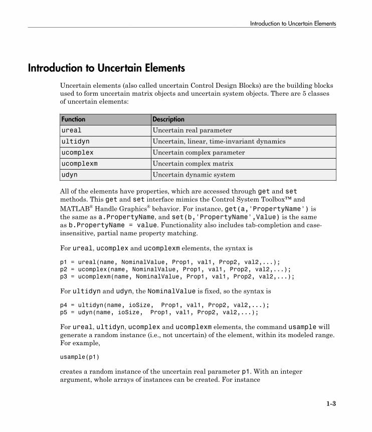
Uncertain elements (also called uncertain Control Design Blocks) are the building blocksused to form uncertain matrix objects and uncertain system objects. There are 5 classesof uncertain elements:
Function Description
ureal Uncertain real parameterultidyn Uncertain, linear, time-invariant dynamicsucomplex Uncertain complex parameterucomplexm Uncertain complex matrixudyn Uncertain dynamic system
All of the elements have properties, which are accessed through get and setmethods. This get and set interface mimics the Control System Toolbox™ andMATLAB® Handle Graphics® behavior. For instance, get(a,'PropertyName') isthe same as a.PropertyName, and set(b,'PropertyName',Value) is the sameas b.PropertyName = value. Functionality also includes tab-completion and case-insensitive, partial name property matching.
For ureal, ucomplex and ucomplexm elements, the syntax is
p1 = ureal(name, NominalValue, Prop1, val1, Prop2, val2,...);
p2 = ucomplex(name, NominalValue, Prop1, val1, Prop2, val2,...);
p3 = ucomplexm(name, NominalValue, Prop1, val1, Prop2, val2,...);
For ultidyn and udyn, the NominalValue is fixed, so the syntax is
p4 = ultidyn(name, ioSize, Prop1, val1, Prop2, val2,...);
p5 = udyn(name, ioSize, Prop1, val1, Prop2, val2,...);
For ureal, ultidyn, ucomplex and ucomplexm elements, the command usample willgenerate a random instance (i.e., not uncertain) of the element, within its modeled range.For example,
usample(p1)
creates a random instance of the uncertain real parameter p1. With an integerargument, whole arrays of instances can be created. For instance
1 Building Uncertain Models
1-4
usample(p4,100)
generates an array of 100 instances of the ultidyn object p4. See “Generate Samples ofUncertain Systems” on page 1-53 to learn more about usample.
Uncertain Real Parameters
1-5
Uncertain Real Parameters
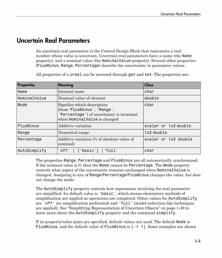
An uncertain real parameter is the Control Design Block that represents a realnumber whose value is uncertain. Uncertain real parameters have a name (the Nameproperty), and a nominal value (the NominalValue property). Several other properties(PlusMinus, Range, Percentage) describe the uncertainty in parameter values.
All properties of a ureal can be accessed through get and set. The properties are:
Properties Meaning Class
Name Internal name char
NominalValue Nominal value of element double
Mode Signifies which description(from'PlusMinus', 'Range','Percentage') of uncertainty is invariantwhen NominalValue is changed
char
PlusMinus Additive variation scalar or 1x2 doubleRange Numerical range 1x2 doublePercentage Additive variation (% of absolute value of
nominal)scalar or 1x2 double
AutoSimplify 'off' | {'basic'} |'full' char
The properties Range, Percentage and PlusMinus are all automatically synchronized.If the nominal value is 0, then the Mode cannot be Percentage. The Mode propertycontrols what aspect of the uncertainty remains unchanged when NominalValue ischanged. Assigning to any of Range/Percentage/PlusMinus changes the value, but doesnot change the mode.
The AutoSimplify property controls how expressions involving the real parameterare simplified. Its default value is 'basic', which means elementary methods ofsimplification are applied as operations are completed. Other values for AutoSimplifyare 'off' (no simplification performed) and 'full' (model-reduction-like techniquesare applied). See “Simplifying Representation of Uncertain Objects” on page 1-49 tolearn more about the AutoSimplify property and the command simplify.
If no property/value pairs are specified, default values are used. The default Mode isPlusMinus, and the default value of PlusMinus is [-1 1]. Some examples are shown
1 Building Uncertain Models
1-6
below. In many cases, the full property name is not specified, taking advantage of thecase-insensitive, partial name property matching.

Create Uncertain Real Parameters
1-7
Create Uncertain Real Parameters
This example shows how to create uncertain real parameters, modify properties such asrange of uncertainty, and sample uncertain parameters.
Create an uncertain real parameter, nominal value 3, with default values for allunspecified properties (including plus/minus variability of 1).
a = ureal('a',3)
a =
Uncertain real parameter "a" with nominal value 3 and variability [-1,1].
View the properties and their values, and note that the Range and Percentagedescriptions of variability are automatically maintained.
get(a)
Name: 'a'
NominalValue: 3
Mode: 'PlusMinus'
Range: [2 4]
PlusMinus: [-1 1]
Percentage: [-33.3333 33.3333]
AutoSimplify: 'basic'
Create an uncertain real parameter, nominal value 2, with 20% variability. Again, viewthe properties, and note that the Range and PlusMinus descriptions of variability areautomatically maintained.
b = ureal('b',2,'Percentage',20)
get(b)
b =
Uncertain real parameter "b" with nominal value 2 and variability [-20,20]%.
Name: 'b'
1 Building Uncertain Models
1-8
NominalValue: 2
Mode: 'Percentage'
Range: [1.6000 2.4000]
PlusMinus: [-0.4000 0.4000]
Percentage: [-20 20]
AutoSimplify: 'basic'
Change the range of the parameter. All descriptions of variability are automaticallyupdated, while the nominal value remains fixed. Although the change in variability wasaccomplished by specifying the Range, the Mode is unaffected, and remains Percentage.
b.Range = [1.9 2.3];
get(b)
Name: 'b'
NominalValue: 2
Mode: 'Percentage'
Range: [1.9000 2.3000]
PlusMinus: [-0.1000 0.3000]
Percentage: [-5.0000 15.0000]
AutoSimplify: 'basic'
As mentioned, the Mode property signifies what aspect of the uncertainty remainsunchanged when NominalValue is modified. Hence, if a real parameter is inPercentage mode, then the Range and PlusMinus properties are determined fromthe Percentage property and NominalValue. Changing NominalValue preserves thePercentage property, and automatically updates the Range and PlusMinus properties.
b.NominalValue = 2.2;
get(b)
Name: 'b'
NominalValue: 2.2000
Mode: 'Percentage'
Range: [2.0900 2.5300]
PlusMinus: [-0.1100 0.3300]
Percentage: [-5.0000 15.0000]
AutoSimplify: 'basic'
Create an uncertain parameter with an asymmetric variation about its nominal value.Examine the properties to confirm the asymmetric range.

Create Uncertain Real Parameters
1-9
c = ureal('c',-5,'Percentage',[-20 30]);
get(c)
Name: 'c'
NominalValue: -5
Mode: 'Percentage'
Range: [-6 -3.5000]
PlusMinus: [-1 1.5000]
Percentage: [-20 30]
AutoSimplify: 'basic'
Create an uncertain parameter, specifying variability with Percentage, but force theMode to be Range.
d = ureal('d',-1,'Mode','Range','Percentage',[-40 60]);
get(d)
Name: 'd'
NominalValue: -1
Mode: 'Range'
Range: [-1.4000 -0.4000]
PlusMinus: [-0.4000 0.6000]
Percentage: [-40 60]
AutoSimplify: 'basic'
Finally, create an uncertain real parameter, and set the AutoSimplify property to'full'.
e = ureal('e',10,'PlusMinus',[-23],'Mode','Percentage','AutoSimplify','Full')
get(e)
e =
Uncertain real parameter "e" with nominal value 10 and variability [-230,230]%.
Name: 'e'
NominalValue: 10
Mode: 'Percentage'
Range: [-13 33]
PlusMinus: [-23 23]
Percentage: [-230 230]

1 Building Uncertain Models
1-10
AutoSimplify: 'full'
Specifying conflicting values for Range/Percentage/PlusMinus when creating aureal element does not result in an error. In this case, the last specified property isused. This last occurrence also determines the Mode, unless Mode is explicitly specified,in which case that is used, regardless of the property/value pairs ordering.
f = ureal('f',3,'PlusMinus',[-2 1],'Percentage',40)
g = ureal('g',2,'PlusMinus',[-2 1],'Mode','Range','Percentage',40)
g.Mode
f =
Uncertain real parameter "f" with nominal value 3 and variability [-40,40]%.
g =
Uncertain real parameter "g" with nominal value 2 and range [1.2,2.8].
ans =
Range
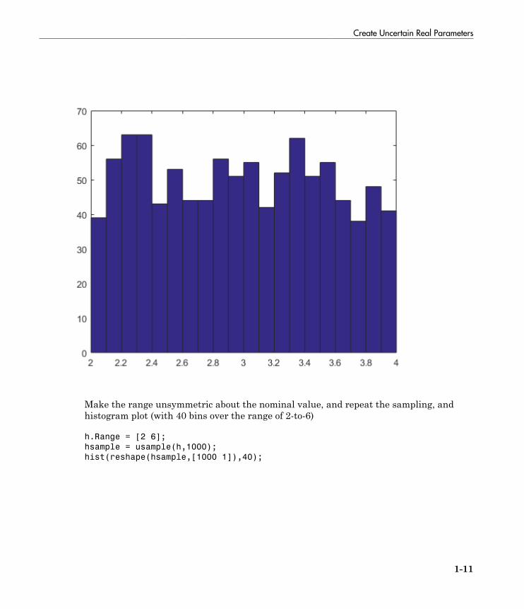
Create an uncertain real parameter, use usample to generate 1000 instances (resultingin a 1-by-1-by-1000 array), reshape the array, and plot a histogram, with 20 bins (withinthe range of 2 to 4).
h = ureal('h',3);
hsample = usample(h,1000);
hist(reshape(hsample,[1000 1]),20);
Create Uncertain Real Parameters
1-11
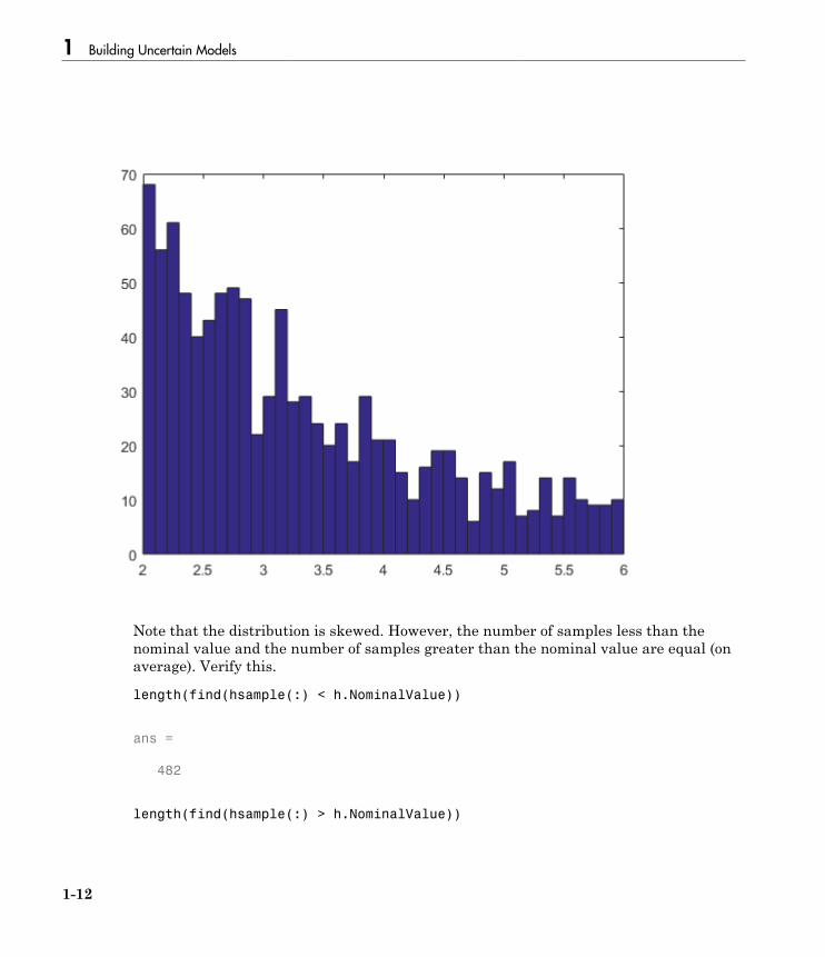
Make the range unsymmetric about the nominal value, and repeat the sampling, andhistogram plot (with 40 bins over the range of 2-to-6)
h.Range = [2 6];
hsample = usample(h,1000);
hist(reshape(hsample,[1000 1]),40);
1 Building Uncertain Models
1-12
Note that the distribution is skewed. However, the number of samples less than thenominal value and the number of samples greater than the nominal value are equal (onaverage). Verify this.
length(find(hsample(:) < h.NominalValue))
ans =
482
length(find(hsample(:) > h.NominalValue))

Create Uncertain Real Parameters
1-13
ans =
518
The distribution used in usample is uniform in the normalized description of theuncertain real parameter. See “Decomposing Uncertain Objects” to learn more about thenormalized description.
There is no notion of an empty ureal (or any other uncertain element, for that matter).ureal, by itself, creates an element named 'UNNAMED', with default property values.
1 Building Uncertain Models
1-14
Uncertain LTI Dynamics Elements
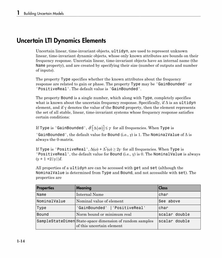
Uncertain linear, time-invariant objects, ultidyn, are used to represent unknownlinear, time-invariant dynamic objects, whose only known attributes are bounds on theirfrequency response. Uncertain linear, time-invariant objects have an internal name (theName property), and are created by specifying their size (number of outputs and numberof inputs).
The property Type specifies whether the known attributes about the frequencyresponse are related to gain or phase. The property Type may be 'GainBounded' or'PositiveReal'. The default value is 'GainBounded'.
The property Bound is a single number, which along with Type, completely specifieswhat is known about the uncertain frequency response. Specifically, if Δ is an ultidynelement, and if γ denotes the value of the Bound property, then the element representsthe set of all stable, linear, time-invariant systems whose frequency response satisfiescertain conditions:
If Type is 'GainBounded', &s w gD ( )ÈÎ ˘ £ for all frequencies. When Type is'GainBounded', the default value for Bound (i.e., γ) is 1. The NominalValue of Δ isalways the 0-matrix.
If Type is 'PositiveReal', Δ(ω) + Δ*(ω) ≥ 2γ· for all frequencies. When Type is'PositiveReal', the default value for Bound (i.e., γ) is 0. The NominalValue is always(γ + 1 +2|γ|)I.
All properties of a ultidyn are can be accessed with get and set (although theNominalValue is determined from Type and Bound, and not accessible with set). Theproperties are
Properties Meaning Class
Name Internal Name char
NominalValue Nominal value of element See above
Type 'GainBounded' |'PositiveReal' char
Bound Norm bound or minimum real scalar double
SampleStateDimensionState-space dimension of random samplesof this uncertain element
scalar double
Uncertain LTI Dynamics Elements
1-15
Properties Meaning Class
SampleMaxFrequencyMaximum natural frequency for randomsampling
scalar double
AutoSimplify 'off' | {'basic'} |'full' char
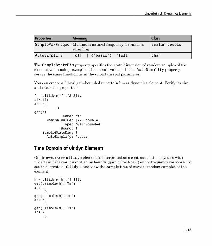
The SampleStateDim property specifies the state dimension of random samples of theelement when using usample. The default value is 1. The AutoSimplify propertyserves the same function as in the uncertain real parameter.
You can create a 2-by-3 gain-bounded uncertain linear dynamics element. Verify its size,and check the properties.
f = ultidyn('f',[2 3]);
size(f)
ans =
2 3
get(f)
Name: 'f'
NominalValue: [2x3 double]
Type: 'GainBounded'
Bound: 1
SampleStateDim: 1
AutoSimplify: 'basic'
Time Domain of ultidyn Elements
On its own, every ultidyn element is interpreted as a continuous-time, system withuncertain behavior, quantified by bounds (gain or real-part) on its frequency response. Tosee this, create a ultidyn, and view the sample time of several random samples of theelement.
h = ultidyn('h',[1 1]);
get(usample(h),'Ts')
ans =
0
get(usample(h),'Ts')
ans =
0
get(usample(h),'Ts')
ans =
0
1 Building Uncertain Models
1-16
However, when a ultidyn element is an uncertain element of an uncertain state spacemodel (uss), then the time-domain characteristic of the element is determined fromthe time-domain characteristic of the system. The bounds (gain-bounded or positivity)apply to the frequency-response of the element. This is explained and demonstrated in“Interpreting Uncertainty in Discrete Time” on page 1-41.
Create Uncertain LTI Dynamics
1-17
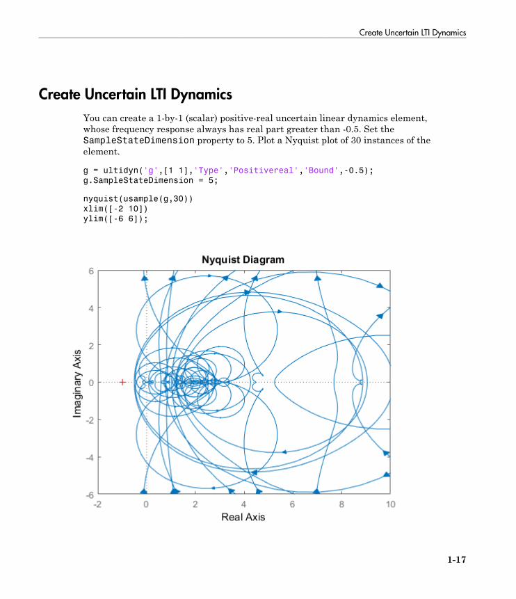
Create Uncertain LTI Dynamics
You can create a 1-by-1 (scalar) positive-real uncertain linear dynamics element,whose frequency response always has real part greater than -0.5. Set theSampleStateDimension property to 5. Plot a Nyquist plot of 30 instances of theelement.
g = ultidyn('g',[1 1],'Type','Positivereal','Bound',-0.5);
g.SampleStateDimension = 5;
nyquist(usample(g,30))
xlim([-2 10])
ylim([-6 6]);
1 Building Uncertain Models
1-18
Uncertain Complex Parameters and Matrices
Uncertain Complex Parameters
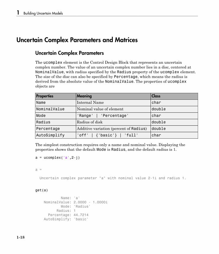
The ucomplex element is the Control Design Block that represents an uncertaincomplex number. The value of an uncertain complex number lies in a disc, centered atNominalValue, with radius specified by the Radius property of the ucomplex element.The size of the disc can also be specified by Percentage, which means the radius isderived from the absolute value of the NominalValue. The properties of ucomplexobjects are
Properties Meaning Class
Name Internal Name char
NominalValue Nominal value of element double
Mode 'Range' | 'Percentage' char
Radius Radius of disk double
Percentage Additive variation (percent of Radius) double
AutoSimplify 'off' | {'basic'} | 'full' char
The simplest construction requires only a name and nominal value. Displaying theproperties shows that the default Mode is Radius, and the default radius is 1.
a = ucomplex('a',2-j)
a =
Uncertain complex parameter "a" with nominal value 2-1i and radius 1.
get(a)
Name: 'a'
NominalValue: 2.0000 - 1.0000i
Mode: 'Radius'
Radius: 1
Percentage: 44.7214
AutoSimplify: 'basic'
Uncertain Complex Parameters and Matrices
1-19
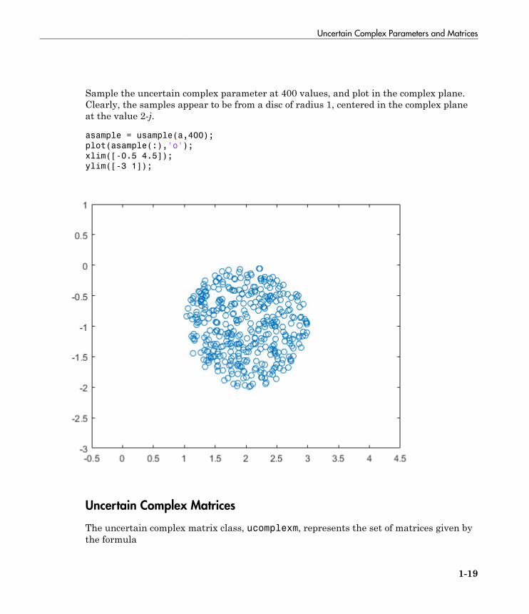
Sample the uncertain complex parameter at 400 values, and plot in the complex plane.Clearly, the samples appear to be from a disc of radius 1, centered in the complex planeat the value 2-j.
asample = usample(a,400);
plot(asample(:),'o');
xlim([-0.5 4.5]);
ylim([-3 1]);
Uncertain Complex Matrices
The uncertain complex matrix class, ucomplexm, represents the set of matrices given bythe formula

1 Building Uncertain Models
1-20
N + WLΔWR
where N, WL, and WR are known matrices, and Δ is any complex matrix with &s D( ) £ 1 .All properties of a ucomplexm are can be accessed with get and set. The properties are
Properties Meaning Class
Name Internal Name char
NominalValue Nominal value of element double
WL Left weight double
WR Right weight double
AutoSimplify 'off' | {'basic'} | 'full' char
The simplest construction requires only a name and nominal value. The default left andright weight matrices are identity.
You can create a 4-by-3 ucomplexm element, and view its properties.
m = ucomplexm('m',[1 2 3;4 5 6;7 8 9;10 11 12])
Uncertain Complex Matrix: Name m, 4x3
get(m)
Name: 'm'
NominalValue: [4x3 double]
WL: [4x4 double]
WR: [3x3 double]
AutoSimplify: 'basic'
m.NominalValue
ans =
1 2 3
4 5 6
7 8 9
10 11 12
m.WL
ans =
1 0 0 0
0 1 0 0
0 0 1 0
0 0 0 1
Sample the uncertain matrix, and compare to the nominal value. Note the element-by-element sizes of the difference are generally equal, indicative of the default (identity)weighting matrices that are in place.

Uncertain Complex Parameters and Matrices
1-21
abs(usample(m)-m.NominalValue)
ans =
0.2948 0.1001 0.2867
0.3028 0.2384 0.2508
0.3376 0.1260 0.2506
0.2200 0.3472 0.1657
Change the left and right weighting matrices, making the uncertainty larger as you movedown the rows, and across the columns.
m.WL = diag([0.2 0.4 0.8 1.6]);
m.WR = diag([0.1 1 4]);
Sample the uncertain matrix, and compare to the nominal value. Note the element-by-element sizes of the difference, and the general trend that the smallest differences arenear the (1,1) element, and the largest differences are near the (4,3) element, which iscompletely expected by choice of the diagonal weighting matrices.
abs(usample(m)-m.NominalValue)
ans =
0.0091 0.0860 0.2753
0.0057 0.1717 0.6413
0.0304 0.2756 1.4012
0.0527 0.4099 1.8335

1 Building Uncertain Models
1-22
Systems with Unmodeled Dynamics
The unstructured uncertain dynamic system Control Design Block, the udyn object,represents completely unknown multivariable, time-varying nonlinear systems.
For practical purposes, these uncertain elements represent noncommuting symbolicvariables (placeholders). All algebraic operations, such as addition, subtraction,multiplication (i.e., cascade) operate properly, and substitution (with usubs) is allowed.However, all of the analysis tools (e.g., robuststab) do not handle these types ofuncertain elements. As such, these elements do not provide a significant amount ofusability, and their role in the user's guide is small.
You can create a 2-by-3 udyn element. Check its size, and properties.
m = udyn('m',[2 3])
m =
Uncertain dynamics "m" with 2 outputs and 3 inputs.
get(m)
NominalValue: [2x3 ss]
AutoSimplify: 'basic'
Ts: 0
TimeUnit: 'seconds'
InputName: {3x1 cell}
InputUnit: {3x1 cell}
InputGroup: [1x1 struct]
OutputName: {2x1 cell}
OutputUnit: {2x1 cell}
OutputGroup: [1x1 struct]
Name: 'm'
Notes: {}
UserData: []
Uncertain Matrices
1-23
Uncertain Matrices
Uncertain matrices (class umat) are built from doubles and uncertain elements,using traditional MATLAB matrix building syntax. Uncertain matrices can be added,subtracted, multiplied, inverted, transposed, etc., resulting in uncertain matrices.The rows and columns of an uncertain matrix are referenced in the same manner thatMATLAB references rows and columns of an array, using parenthesis, and integerindices. The NominalValue of a uncertain matrix is the result obtained when alluncertain elements are replaced with their own NominalValue. The uncertain elementsmaking up a umat are accessible through the Uncertainty gateway, and the propertiesof each element within a umat can be changed directly.
Using usubs, specific values may be substituted for any of the uncertain elements withina umat. The command usample generates a random sample of the uncertain matrix,substituting random samples (within their ranges) for each of the uncertain elements.
The command wcnorm computes tight bounds on the worst-case (maximum over theuncertain elements' ranges) norm of the uncertain matrix.
Standard MATLAB numerical matrices (i.e., double) naturally can be viewed asuncertain matrices without any uncertainty.
1 Building Uncertain Models
1-24
Create Uncertain Matrices from Uncertain Elements
You can create 2 uncertain real parameters, and then a 3-by-2 uncertain matrix usingthese uncertain elements.
a = ureal('a',3);
b = ureal('b',10,'pe',20);
M = [-a 1/b;b a+1/b;1 3]
M =
Uncertain matrix with 3 rows and 2 columns.
The uncertainty consists of the following blocks:
a: Uncertain real, nominal = 3, variability = [-1,1], 2 occurrences
b: Uncertain real, nominal = 10, variability = [-20,20]%, 3 occurrences
Type "M.NominalValue" to see the nominal value, "get(M)" to see all properties, and "M.Uncertainty" to interact with the uncertain elements.
Access Properties of a umat
1-25
Access Properties of a umat
Use get to view the accessible properties of a umat.
get(M)
NominalValue: [3x2 double]
Uncertainty: [1x1 elementlist]
The NominalValue is a double, obtained by replacing all uncertain elements with theirnominal values.
M.NominalValue
ans =
-3.0000 0.1000
10.0000 3.1000
1.0000 3.0000
The Uncertainty property is a structure, whose fields are the uncertain elements(Control Design Blocks) of M.
M.Uncertainty
ans =
a: [1x1 ureal]
b: [1x1 ureal]
M.Uncertainty.a
ans =
Uncertain real parameter "a" with nominal value 3 and variability [-1,1].
Direct access to the elements is facilitated through Uncertainty. Check the Range ofthe uncertain element named 'a' within M, then change it.
M.Uncertainty.a.Range
ans =
2 4
M.Uncertainty.a.Range = [2.5 5];
M
UMAT: 3 Rows, 2 Columns
a: real, nominal = 3, variability = [-0.5 2], 2 occurrences
b: real, nominal = 10, variability = [-20 20]%, 3 occurrences

1 Building Uncertain Models
1-26
The change to the uncertain real parameter a only took place within M. Verify that thevariable a in the workspace is no longer the same as the variable a within M.
isequal(M.Uncertainty.a,a)
ans =
0
Note that combining elements which have a common internal name, but differentproperties leads to an error. For instance, subtracting the two elements gives an error,not 0.
M.Uncertainty.a - a
??? Error using ==> ndlft.lftmask
Elements named 'a' have different properties.
Row and Column Referencing
1-27
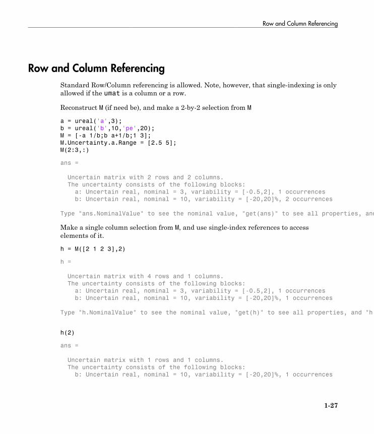
Row and Column Referencing
Standard Row/Column referencing is allowed. Note, however, that single-indexing is onlyallowed if the umat is a column or a row.
Reconstruct M (if need be), and make a 2-by-2 selection from M
a = ureal('a',3);
b = ureal('b',10,'pe',20);
M = [-a 1/b;b a+1/b;1 3];
M.Uncertainty.a.Range = [2.5 5];
M(2:3,:)
ans =
Uncertain matrix with 2 rows and 2 columns.
The uncertainty consists of the following blocks:
a: Uncertain real, nominal = 3, variability = [-0.5,2], 1 occurrences
b: Uncertain real, nominal = 10, variability = [-20,20]%, 2 occurrences
Type "ans.NominalValue" to see the nominal value, "get(ans)" to see all properties, and "ans.Uncertainty" to interact with the uncertain elements.
Make a single column selection from M, and use single-index references to accesselements of it.
h = M([2 1 2 3],2)
h =
Uncertain matrix with 4 rows and 1 columns.
The uncertainty consists of the following blocks:
a: Uncertain real, nominal = 3, variability = [-0.5,2], 1 occurrences
b: Uncertain real, nominal = 10, variability = [-20,20]%, 1 occurrences
Type "h.NominalValue" to see the nominal value, "get(h)" to see all properties, and "h.Uncertainty" to interact with the uncertain elements.
h(2)
ans =
Uncertain matrix with 1 rows and 1 columns.
The uncertainty consists of the following blocks:
b: Uncertain real, nominal = 10, variability = [-20,20]%, 1 occurrences
1 Building Uncertain Models
1-28
Type "ans.NominalValue" to see the nominal value, "get(ans)" to see all properties, and "ans.Uncertainty" to interact with the uncertain elements.
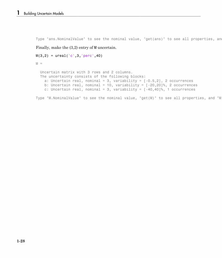
Finally, make the (3,2) entry of M uncertain.
M(3,2) = ureal('c',3,'perc',40)
M =
Uncertain matrix with 3 rows and 2 columns.
The uncertainty consists of the following blocks:
a: Uncertain real, nominal = 3, variability = [-0.5,2], 2 occurrences
b: Uncertain real, nominal = 10, variability = [-20,20]%, 2 occurrences
c: Uncertain real, nominal = 3, variability = [-40,40]%, 1 occurrences
Type "M.NominalValue" to see the nominal value, "get(M)" to see all properties, and "M.Uncertainty" to interact with the uncertain elements.
Matrix Operation on umat Objects
1-29
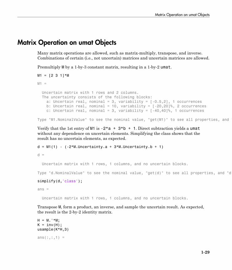
Matrix Operation on umat Objects
Many matrix operations are allowed, such as matrix-multiply, transpose, and inverse.Combinations of certain (i.e., not uncertain) matrices and uncertain matrices are allowed.
Premultiply M by a 1-by-3 constant matrix, resulting in a 1-by-2 umat.
M1 = [2 3 1]*M
M1 =
Uncertain matrix with 1 rows and 2 columns.
The uncertainty consists of the following blocks:
a: Uncertain real, nominal = 3, variability = [-0.5,2], 1 occurrences
b: Uncertain real, nominal = 10, variability = [-20,20]%, 2 occurrences
c: Uncertain real, nominal = 3, variability = [-40,40]%, 1 occurrences
Type "M1.NominalValue" to see the nominal value, "get(M1)" to see all properties, and "M1.Uncertainty" to interact with the uncertain elements.
Verify that the 1st entry of M1 is -2*a + 3*b + 1. Direct subtraction yields a umatwithout any dependence on uncertain elements. Simplifying the class shows that theresult has no uncertain elements, as expected.
d = M1(1) - (-2*M.Uncertainty.a + 3*M.Uncertainty.b + 1)
d =
Uncertain matrix with 1 rows, 1 columns, and no uncertain blocks.
Type "d.NominalValue" to see the nominal value, "get(d)" to see all properties, and "d.Uncertainty" to interact with the uncertain elements.
simplify(d,'class');
ans =
Uncertain matrix with 1 rows, 1 columns, and no uncertain blocks.
Transpose M, form a product, an inverse, and sample the uncertain result. As expected,the result is the 2-by-2 identity matrix.
H = M.'*M;
K = inv(H);
usample(K*H,3)
ans(:,:,1) =
1 Building Uncertain Models
1-30
1.0000 -0.0000
-0.0000 1.0000
ans(:,:,2) =
1.0000 0.0000
-0.0000 1.0000
ans(:,:,3) =
1.0000 0.0000
-0.0000 1.0000
Evaluate Uncertain Elements by Substitution
1-31
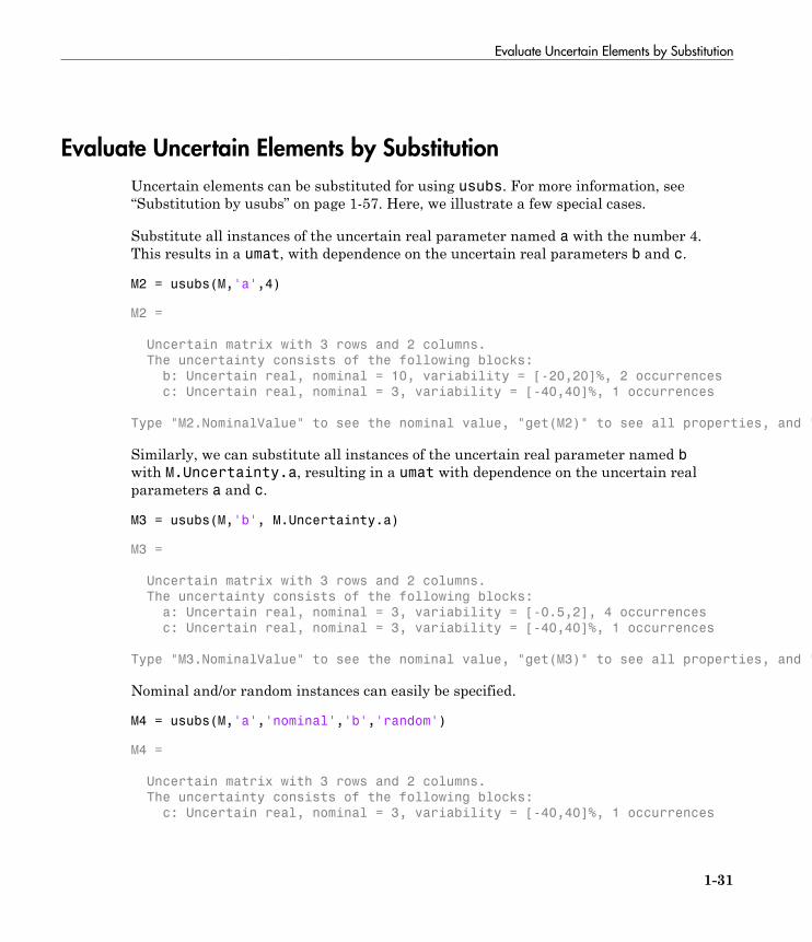
Evaluate Uncertain Elements by Substitution
Uncertain elements can be substituted for using usubs. For more information, see“Substitution by usubs” on page 1-57. Here, we illustrate a few special cases.
Substitute all instances of the uncertain real parameter named a with the number 4.This results in a umat, with dependence on the uncertain real parameters b and c.
M2 = usubs(M,'a',4)
M2 =
Uncertain matrix with 3 rows and 2 columns.
The uncertainty consists of the following blocks:
b: Uncertain real, nominal = 10, variability = [-20,20]%, 2 occurrences
c: Uncertain real, nominal = 3, variability = [-40,40]%, 1 occurrences
Type "M2.NominalValue" to see the nominal value, "get(M2)" to see all properties, and "M2.Uncertainty" to interact with the uncertain elements.
Similarly, we can substitute all instances of the uncertain real parameter named bwith M.Uncertainty.a, resulting in a umat with dependence on the uncertain realparameters a and c.
M3 = usubs(M,'b', M.Uncertainty.a)
M3 =
Uncertain matrix with 3 rows and 2 columns.
The uncertainty consists of the following blocks:
a: Uncertain real, nominal = 3, variability = [-0.5,2], 4 occurrences
c: Uncertain real, nominal = 3, variability = [-40,40]%, 1 occurrences
Type "M3.NominalValue" to see the nominal value, "get(M3)" to see all properties, and "M3.Uncertainty" to interact with the uncertain elements.
Nominal and/or random instances can easily be specified.
M4 = usubs(M,'a','nominal','b','random')
M4 =
Uncertain matrix with 3 rows and 2 columns.
The uncertainty consists of the following blocks:
c: Uncertain real, nominal = 3, variability = [-40,40]%, 1 occurrences
1 Building Uncertain Models
1-32
Type "M4.NominalValue" to see the nominal value, "get(M4)" to see all properties, and "M4.Uncertainty" to interact with the uncertain elements.
The command usample also generates multiple random instances of a umat (and ussand ufrd). See “Generate Samples of Uncertain Systems” on page 1-53 for details.
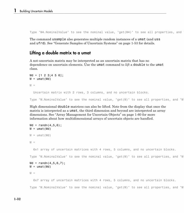
Lifting a double matrix to a umat
A not-uncertain matrix may be interpreted as an uncertain matrix that has nodependence on uncertain elements. Use the umat command to lift a double to the umatclass.
Md = [1 2 3;4 5 6];
M = umat(Md)
M =
Uncertain matrix with 2 rows, 3 columns, and no uncertain blocks.
Type "M.NominalValue" to see the nominal value, "get(M)" to see all properties, and "M.Uncertainty" to interact with the uncertain elements.
High dimensional double matrices can also be lifted. Note from the display that once thematrix is interpreted as a umat, the third dimension and beyond are interpreted as arraydimensions. See “Array Management for Uncertain Objects” on page 1-60 for moreinformation about how multidimensional arrays of uncertain objects are handled.
Md = randn(4,5,6);
M = umat(Md)
M = umat(Md)
M =
6x1 array of uncertain matrices with 4 rows, 5 columns, and no uncertain blocks.
Type "M.NominalValue" to see the nominal value, "get(M)" to see all properties, and "M.Uncertainty" to interact with the uncertain elements.
Md = randn(4,5,6,7);
M = umat(Md)
M =
6x7 array of uncertain matrices with 4 rows, 5 columns, and no uncertain blocks.
Type "M.NominalValue" to see the nominal value, "get(M)" to see all properties, and "M.Uncertainty" to interact with the uncertain elements.
Uncertain State-Space Models (uss)
1-33
Uncertain State-Space Models (uss)
Uncertain systems (uss) are linear systems with uncertain state-space matrices and/or uncertain linear dynamics. Like their certain (i.e., not uncertain) counterpart, the ssobject, they are often built from state-space matrices using the ss command. In the casewhere some of the state-space matrices are uncertain elements (uncertain Control DesignBlocks), the result will be a uncertain state-space (uss) object.
Combining uncertain systems with uncertain systems (with the feedback command, forexample) usually leads to an uncertain system. Not-uncertain systems can be combinedwith uncertain systems. Usually the result is an uncertain system.
The nominal value of an uncertain system is a ss object, which is familiar to ControlSystem Toolbox software users.
Properties of uss Objects
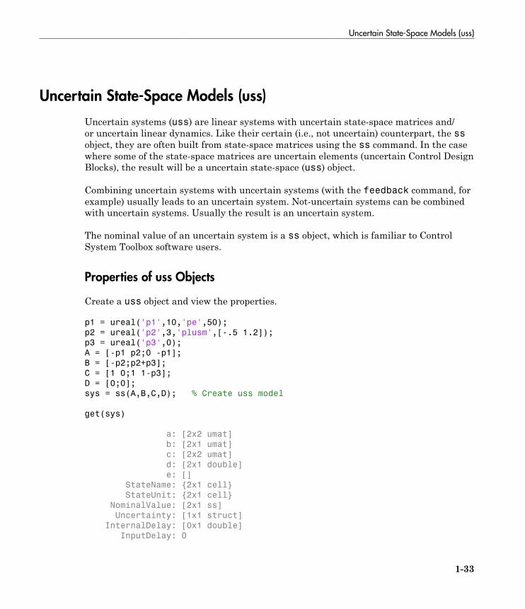
Create a uss object and view the properties.
p1 = ureal('p1',10,'pe',50);
p2 = ureal('p2',3,'plusm',[-.5 1.2]);
p3 = ureal('p3',0);
A = [-p1 p2;0 -p1];
B = [-p2;p2+p3];
C = [1 0;1 1-p3];
D = [0;0];
sys = ss(A,B,C,D); % Create uss model
get(sys)
a: [2x2 umat]
b: [2x1 umat]
c: [2x2 umat]
d: [2x1 double]
e: []
StateName: {2x1 cell}
StateUnit: {2x1 cell}
NominalValue: [2x1 ss]
Uncertainty: [1x1 struct]
InternalDelay: [0x1 double]
InputDelay: 0
1 Building Uncertain Models
1-34
OutputDelay: [2x1 double]
Ts: 0
TimeUnit: 'seconds'
InputName: {''}
InputUnit: {''}
InputGroup: [1x1 struct]
OutputName: {2x1 cell}
OutputUnit: {2x1 cell}
OutputGroup: [1x1 struct]
Name: ''
Notes: {}
UserData: []
SamplingGrid: [1x1 struct]
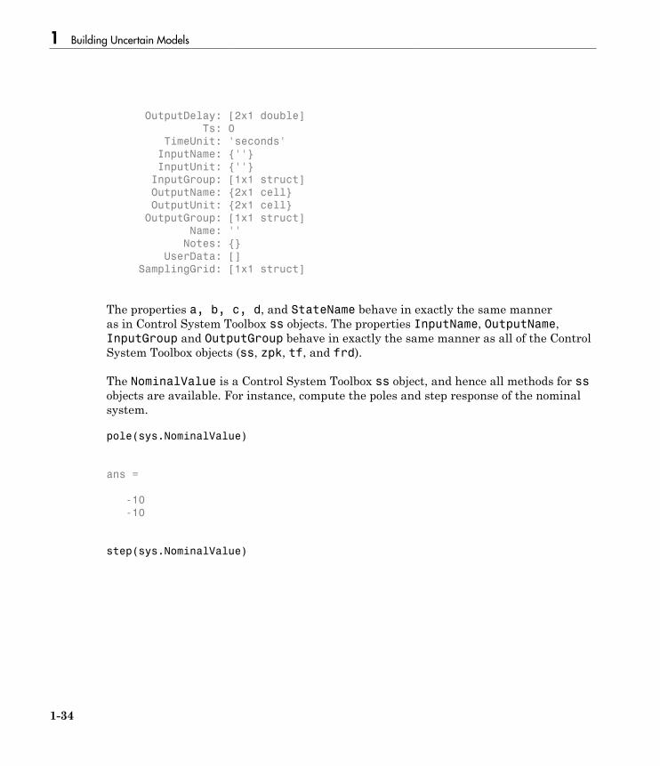
The properties a, b, c, d, and StateName behave in exactly the same manneras in Control System Toolbox ss objects. The properties InputName, OutputName,InputGroup and OutputGroup behave in exactly the same manner as all of the ControlSystem Toolbox objects (ss, zpk, tf, and frd).
The NominalValue is a Control System Toolbox ss object, and hence all methods for ssobjects are available. For instance, compute the poles and step response of the nominalsystem.
pole(sys.NominalValue)
ans =
-10
-10
step(sys.NominalValue)
Uncertain State-Space Models (uss)
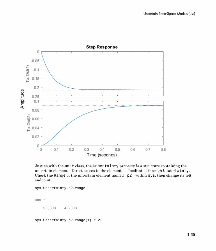
1-35
Just as with the umat class, the Uncertainty property is a structure containing theuncertain elements. Direct access to the elements is facilitated through Uncertainty.Check the Range of the uncertain element named 'p2' within sys, then change its leftendpoint.
sys.Uncertainty.p2.range
ans =
2.5000 4.2000
sys.Uncertainty.p2.range(1) = 2;
1 Building Uncertain Models
1-36
Create Uncertain State-Space Model
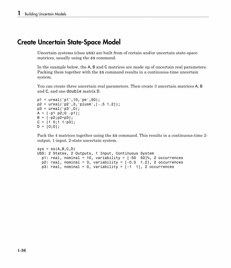
Uncertain systems (class uss) are built from of certain and/or uncertain state-spacematrices, usually using the ss command.
In the example below, the A, B and C matrices are made up of uncertain real parameters.Packing them together with the ss command results in a continuous-time uncertainsystem.
You can create three uncertain real parameters. Then create 3 uncertain matrices A, Band C, and one double matrix D.
p1 = ureal('p1',10,'pe',50);
p2 = ureal('p2',3,'plusm',[-.5 1.2]);
p3 = ureal('p3',0);
A = [-p1 p2;0 -p1];
B = [-p2;p2+p3];
C = [1 0;1 1-p3];
D = [0;0];
Pack the 4 matrices together using the ss command. This results in a continuous-time 2-output, 1-input, 2-state uncertain system.
sys = ss(A,B,C,D)
USS: 2 States, 2 Outputs, 1 Input, Continuous System
p1: real, nominal = 10, variability = [-50 50]%, 2 occurrences
p2: real, nominal = 3, variability = [-0.5 1.2], 2 occurrences
p3: real, nominal = 0, variability = [-1 1], 2 occurrences

Sample Uncertain Systems
1-37
Sample Uncertain Systems
The command usample randomly samples the uncertain system at a specified numberof points. Randomly sample an uncertain system at 20 points in its modeled uncertaintyrange. This gives a 20-by-1 ss array. Consequently, all analysis tools from ControlSystem Toolbox™ are available.
p1 = ureal('p1',10,'Percentage',50);
p2 = ureal('p2',3,'PlusMinus',[-.5 1.2]);
p3 = ureal('p3',0);
A = [-p1 p2; 0 -p1];
B = [-p2; p2+p3];
C = [1 0; 1 1-p3];
D = [0; 0];
sys = ss(A,B,C,D) % Create uncertain state-space model
sys =
Uncertain continuous-time state-space model with 2 outputs, 1 inputs, 2 states.
The model uncertainty consists of the following blocks:
p1: Uncertain real, nominal = 10, variability = [-50,50]%, 2 occurrences
p2: Uncertain real, nominal = 3, variability = [-0.5,1.2], 2 occurrences
p3: Uncertain real, nominal = 0, variability = [-1,1], 2 occurrences
Type "sys.NominalValue" to see the nominal value, "get(sys)" to see all properties, and "sys.Uncertainty" to interact with the uncertain elements.
manysys = usample(sys,20);
size(manysys)
20x1 array of state-space models.
Each model has 2 outputs, 1 inputs, and 2 states.
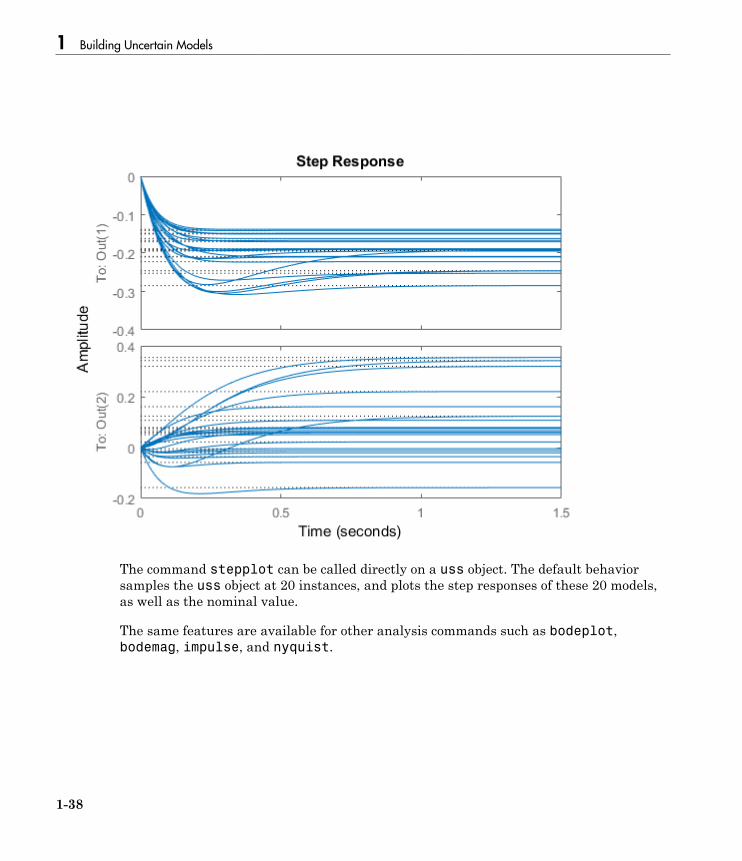
stepplot(manysys)
1 Building Uncertain Models
1-38
The command stepplot can be called directly on a uss object. The default behaviorsamples the uss object at 20 instances, and plots the step responses of these 20 models,as well as the nominal value.
The same features are available for other analysis commands such as bodeplot,bodemag, impulse, and nyquist.
Feedback Around an Uncertain Plant
1-39
Feedback Around an Uncertain Plant
It is possible to form interconnections of uss objects. A common example is to form thefeedback interconnection of a given controller with an uncertain plant.
First create the uncertain plant. Start with two uncertain real parameters.
gamma = ureal('gamma',4);
tau = ureal('tau',.5,'Percentage',30);
Next, create an unmodeled dynamics element, delta, and a first-order weightingfunction, whose DC value is 0.2, high-frequency gain is 10, and whose crossoverfrequency is 8 rad/sec.
delta = ultidyn('delta',[1 1],'SampleStateDimension',5);
W = makeweight(0.2,6,6);
Finally, create the uncertain plant consisting of the uncertain parameters and theunmodeled dynamics.
P = tf(gamma,[tau 1])*(1+W*delta);
You can create an integral controller based on nominal plant parameters. Nominally theclosed-loop system will have damping ratio of 0.707 and time constant of 2*tau.
KI = 1/(2*tau.Nominal*gamma.Nominal);
C = tf(KI,[1 0]);
Create the uncertain closed-loop system using the feedback command.
CLP = feedback(P*C,1);
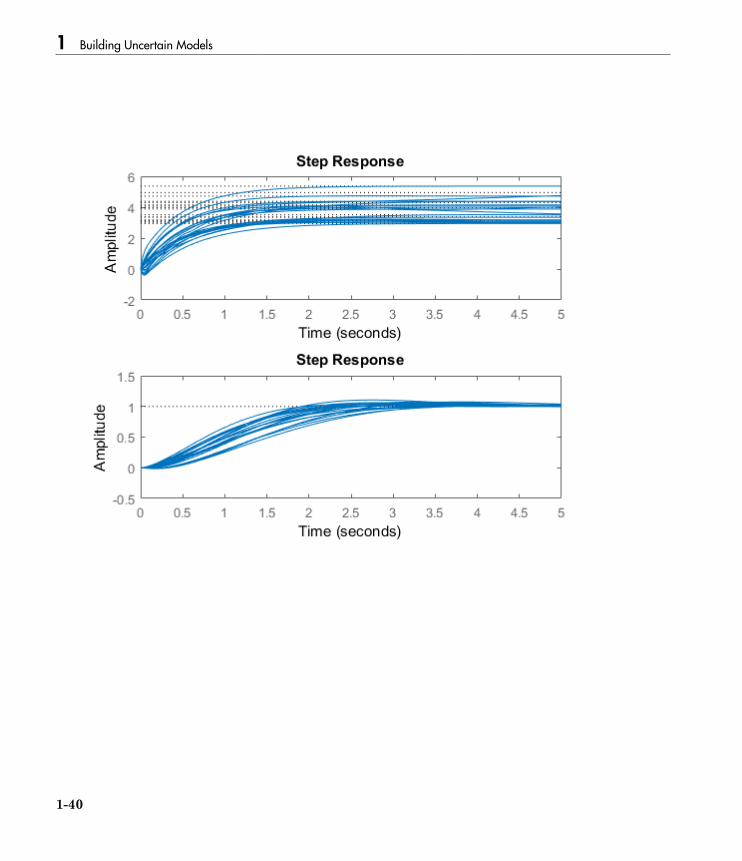
Plot samples of the open-loop and closed-loop step responses. As expected the integralcontroller reduces the variability in the low frequency response.
subplot(2,1,1);
stepplot(P,5)
subplot(2,1,2);
stepplot(CLP,5)
1 Building Uncertain Models
1-40

Interpreting Uncertainty in Discrete Time
1-41
Interpreting Uncertainty in Discrete Time
The interpretation of a ultidyn element as a continuous-time or discrete-time systemdepends on the nature of the uncertain system (uss) within which it is an uncertainelement.
For example, create a scalar ultidyn object. Then, create two 1-input, 1-output ussobjects using the ultidyn object as their “D” matrix. In one case, create withoutspecifying sample-time, which indicates continuous time. In the second case, forcediscrete-time, with a sample time of 0.42.
delta = ultidyn('delta',[1 1]);
sys1 = uss([],[],[],delta)
USS: 0 States, 1 Output, 1 Input, Continuous System
delta: 1x1 LTI, max. gain = 1, 1 occurrence
sys2 = uss([],[],[],delta,0.42)
USS: 0 States, 1 Output, 1 Input, Discrete System, Ts = 0.42
delta: 1x1 LTI, max. gain = 1, 1 occurrence
Next, get a random sample of each system. When obtaining random samples usingusample, the values of the elements used in the sample are returned in the 2ndargument from usample as a structure.
[sys1s,d1v] = usample(sys1);
[sys2s,d2v] = usample(sys2);
Look at d1v.delta.Ts and d2v.delta.Ts. In the first case, since sys1 is continuous-time, the system d1v.delta is continuous-time. In the second case, since sys2 isdiscrete-time, with sample time 0.42, the system d2v.delta is discrete-time, withsample time 0.42.
d1v.delta.Ts
ans =
0
d2v.delta.Ts
ans =
0.4200
Finally, in the case of a discrete-time uss object, it is not the case that ultidyn objectsare interpreted as continuous-time uncertainty in feedback with sampled-data systems.This very interesting hybrid theory is beyond the scope of the toolbox.
1 Building Uncertain Models
1-42
Lifting a ss to a uss
A not-uncertain state space object may be interpreted as an uncertain state space objectthat has no dependence on uncertain elements. Use the uss command to “lift” a ss to theuss class.
sys = rss(3,2,1);
usys = uss(sys)
USS: 3 States, 2 Outputs, 1 Input, Continuous System
Arrays of ss objects can also be lifted. See “Array Management for Uncertain Objects” onpage 1-60 for more information about how arrays of uncertain objects are handled.
Create Uncertain Frequency Response Data Models
1-43
Create Uncertain Frequency Response Data Models
Uncertain frequency responses (ufrd) arise naturally when computing the frequencyresponse of an uncertain state-space (uss). They also arise when frequency responsedata (in an frd model object) is combined (added, multiplied, concatenated, etc.) to anuncertain matrix (umat).
The most common manner in which a ufrd arises is taking the frequency response of auss. To do this, use the ufrd command.
Construct an uncertain state-space model sys.
p1 = ureal('p1',10,'pe',50);
p2 = ureal('p2',3,'plusm',[-.5 1.2]);
p3 = ureal('p3',0);
A = [-p1 p2;0 -p1];
B = [-p2;p2+p3];
C = [1 0;1 1-p3];
D = [0;0];
sys = ss(A,B,C,D)
sys =
Uncertain continuous-time state-space model with 2 outputs, 1 inputs, 2 states.
The model uncertainty consists of the following blocks:
p1: Uncertain real, nominal = 10, variability = [-50,50]%, 2 occurrences
p2: Uncertain real, nominal = 3, variability = [-0.5,1.2], 2 occurrences
p3: Uncertain real, nominal = 0, variability = [-1,1], 2 occurrences
Type "sys.NominalValue" to see the nominal value, "get(sys)" to see all properties, and "sys.Uncertainty" to interact with the uncertain elements.
Compute the uncertain frequency response of the uncertain system. Use the ufrdcommand, along with a frequency grid containing 100 points. The result is an uncertainfrequency response data object, referred to as a ufrd model.
sysg = ufrd(sys,logspace(-2,2,100))
Uncertain continuous-time FRD model with 2 outputs, 1 inputs, 100 frequency points.
p1: Uncertain real, nominal = 10, variability = [-50,50]%, 2 occurrences
p2: Uncertain real, nominal = 3, variability = [-0.5,1.2], 2 occurrences
p3: Uncertain real, nominal = 0, variability = [-1,1], 2 occurrences
Type "sysg.NominalValue" to see the nominal value, "get(sysg)" to see all properties, and "sysg.Uncertainty" to interact with the uncertain elements.

1 Building Uncertain Models
1-44
Properties of ufrd Objects
View the properties with the get command.
get(sysg)
Frequency: [100x1 double]
FrequencyUnit: 'rad/TimeUnit'
ResponseData: [4-D umat]
NominalValue: [2x1 frd]
Uncertainty: [1x1 struct]
InputDelay: 0
OutputDelay: [2x1 double]
Ts: 0
TimeUnit: 'seconds'
InputName: {''}
InputUnit: {''}
InputGroup: [1x1 struct]
OutputName: {2x1 cell}
OutputUnit: {2x1 cell}
OutputGroup: [1x1 struct]
Name: ''
Notes: {}
UserData: []
The properties ResponseData and Frequency behave in exactly the same manneras Control System Toolbox frd objects, except that ResponseData is a umat. Theproperties InputName, OutputName, InputGroup and OutputGroup behave inexactly the same manner as all of the Control System Toolbox objects (ss, zpk, tf andfrd).
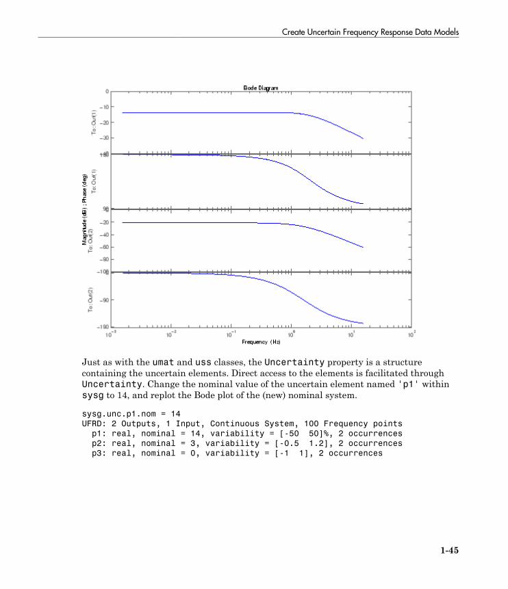
The NominalValue is a Control System Toolbox frd object, and hence all methods forfrd objects are available. For instance, plot the Bode response of the nominal system.
bode(sysg.nom)
Create Uncertain Frequency Response Data Models
1-45
Just as with the umat and uss classes, the Uncertainty property is a structurecontaining the uncertain elements. Direct access to the elements is facilitated throughUncertainty. Change the nominal value of the uncertain element named 'p1' withinsysg to 14, and replot the Bode plot of the (new) nominal system.
sysg.unc.p1.nom = 14
UFRD: 2 Outputs, 1 Input, Continuous System, 100 Frequency points
p1: real, nominal = 14, variability = [-50 50]%, 2 occurrences
p2: real, nominal = 3, variability = [-0.5 1.2], 2 occurrences
p3: real, nominal = 0, variability = [-1 1], 2 occurrences
1 Building Uncertain Models
1-46
Interpreting Uncertainty in Discrete Time
See “Interpreting Uncertainty in Discrete Time” on page 1-41. The issues are identical.

Lifting an frd to a ufrd
1-47
Lifting an frd to a ufrd
A not-uncertain frequency response object may be interpreted as an uncertain frequencyresponse object that has no dependence on uncertain elements. Use the ufrd commandto “lift” an frd object to the ufrd class.
sys = rss(3,2,1);
sysg = frd(sys,logspace(-2,2,100));
usysg = ufrd(sysg)
UFRD: 2 Outputs, 1 Input, Continuous System, 100 Frequency points
Arrays of frd objects can also be lifted. See “Array Management for Uncertain Objects”on page 1-60 for more information about how arrays of uncertain objects are handled.
1 Building Uncertain Models
1-48
Basic Control System Toolbox and MATLAB Interconnections
This list has all of the basic system interconnection functions defined in Control SystemToolbox software or in MATLAB.
• append
• blkdiag
• series
• parallel
• feedback
• lft
• stack
These functions work with uncertain objects as well. Uncertain objects may be combinedwith certain objects, resulting in an uncertain object.

Simplifying Representation of Uncertain Objects
1-49
Simplifying Representation of Uncertain Objects
A minimal realization of the transfer function matrix
H ss s
s s
( ) = + +
+ +
È
Î
ÍÍÍÍ
˘
˚
˙˙˙˙
2
1
4
1
3
1
6
1
has only 1 state, obvious from the decomposition
H ss
( ) =È
ÎÍ
˘
˚˙ +
[ ]2
3
1
11 2 .
However, a “natural” construction, formed by
sys11 = ss(tf(2,[1 1]));
sys12 = ss(tf(4,[1 1]));
sys21 = ss(tf(3,[1 1]));
sys22 = ss(tf(6,[1 1]));
sys = [sys11 sys12;sys21 sys22]
a =
x1 x2 x3 x4
x1 -1 0 0 0
x2 0 -1 0 0
x3 0 0 -1 0
x4 0 0 0 -1
b =
u1 u2
x1 2 0
x2 0 2
x3 2 0
x4 0 2
c =
x1 x2 x3 x4
y1 1 2 0 0
y2 0 0 1.5 3
d =
u1 u2
y1 0 0
y2 0 0
1 Building Uncertain Models
1-50
Continuous-time model
has four states, and is nonminimal.
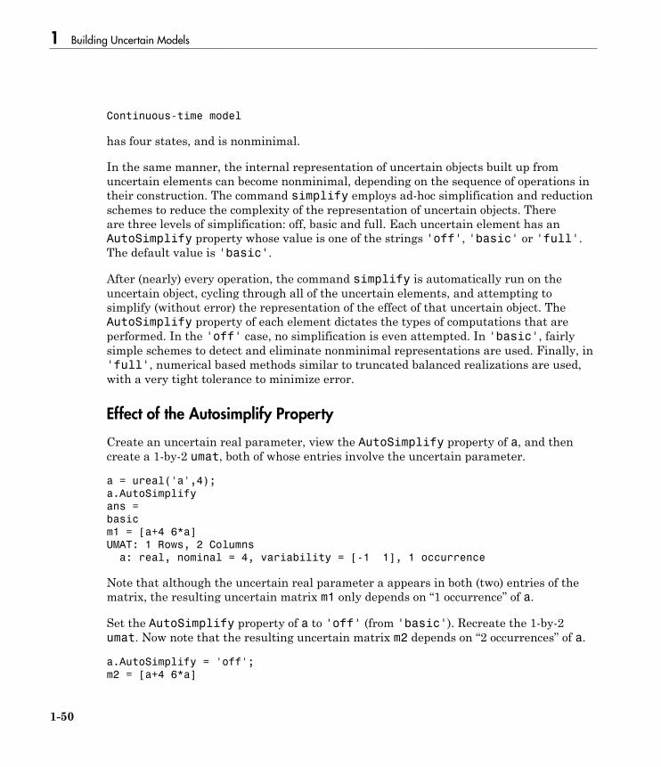
In the same manner, the internal representation of uncertain objects built up fromuncertain elements can become nonminimal, depending on the sequence of operations intheir construction. The command simplify employs ad-hoc simplification and reductionschemes to reduce the complexity of the representation of uncertain objects. Thereare three levels of simplification: off, basic and full. Each uncertain element has anAutoSimplify property whose value is one of the strings 'off', 'basic' or 'full'.The default value is 'basic'.
After (nearly) every operation, the command simplify is automatically run on theuncertain object, cycling through all of the uncertain elements, and attempting tosimplify (without error) the representation of the effect of that uncertain object. TheAutoSimplify property of each element dictates the types of computations that areperformed. In the 'off' case, no simplification is even attempted. In 'basic', fairlysimple schemes to detect and eliminate nonminimal representations are used. Finally, in'full', numerical based methods similar to truncated balanced realizations are used,with a very tight tolerance to minimize error.
Effect of the Autosimplify Property
Create an uncertain real parameter, view the AutoSimplify property of a, and thencreate a 1-by-2 umat, both of whose entries involve the uncertain parameter.
a = ureal('a',4);
a.AutoSimplify
ans =
basic
m1 = [a+4 6*a]
UMAT: 1 Rows, 2 Columns
a: real, nominal = 4, variability = [-1 1], 1 occurrence
Note that although the uncertain real parameter a appears in both (two) entries of thematrix, the resulting uncertain matrix m1 only depends on “1 occurrence” of a.
Set the AutoSimplify property of a to 'off' (from 'basic'). Recreate the 1-by-2umat. Now note that the resulting uncertain matrix m2 depends on “2 occurrences” of a.
a.AutoSimplify = 'off';
m2 = [a+4 6*a]
Simplifying Representation of Uncertain Objects
1-51
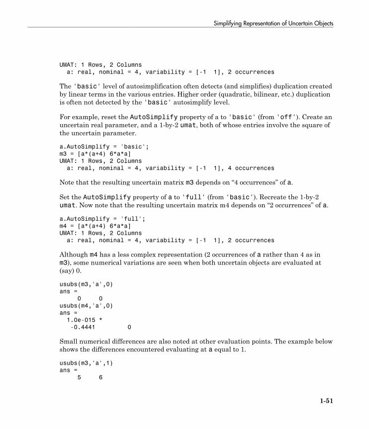
UMAT: 1 Rows, 2 Columns
a: real, nominal = 4, variability = [-1 1], 2 occurrences
The 'basic' level of autosimplification often detects (and simplifies) duplication createdby linear terms in the various entries. Higher order (quadratic, bilinear, etc.) duplicationis often not detected by the 'basic' autosimplify level.
For example, reset the AutoSimplify property of a to 'basic' (from 'off'). Create anuncertain real parameter, and a 1-by-2 umat, both of whose entries involve the square ofthe uncertain parameter.
a.AutoSimplify = 'basic';
m3 = [a*(a+4) 6*a*a]
UMAT: 1 Rows, 2 Columns
a: real, nominal = 4, variability = [-1 1], 4 occurrences
Note that the resulting uncertain matrix m3 depends on “4 occurrences” of a.
Set the AutoSimplify property of a to 'full' (from 'basic'). Recreate the 1-by-2umat. Now note that the resulting uncertain matrix m4 depends on “2 occurrences” of a.
a.AutoSimplify = 'full';
m4 = [a*(a+4) 6*a*a]
UMAT: 1 Rows, 2 Columns
a: real, nominal = 4, variability = [-1 1], 2 occurrences
Although m4 has a less complex representation (2 occurrences of a rather than 4 as inm3), some numerical variations are seen when both uncertain objects are evaluated at(say) 0.
usubs(m3,'a',0)
ans =
0 0
usubs(m4,'a',0)
ans =
1.0e-015 *
-0.4441 0
Small numerical differences are also noted at other evaluation points. The example belowshows the differences encountered evaluating at a equal to 1.
usubs(m3,'a',1)
ans =
5 6
1 Building Uncertain Models
1-52
usubs(m4,'a',1)
ans =
5.0000 6.0000
Direct Use of simplify
The simplify command can be used to override all uncertain element's AutoSimplifyproperty. The first input to the simplify command is an uncertain object. The secondinput is the desired reduction technique, which can either 'basic' or 'full'.
Again create an uncertain real parameter, and a 1-by-2 umat, both of whose entriesinvolve the square of the uncertain parameter. Set the AutoSimplify property of a to'basic'.
a.AutoSimplify = 'basic';
m3 = [a*(a+4) 6*a*a]
UMAT: 1 Rows, 2 Columns
a: real, nominal = 4, variability = [-1 1], 4 occurrences
Note that the resulting uncertain matrix m3 depends on four occurrences of a.
The simplify command can be used to perform a 'full' reduction on the resultingumat.
m4 = simplify(m3,'full')
UMAT: 1 Rows, 2 Columns
a: real, nominal = 4, variability = [-1 1], 2 occurrences
The resulting uncertain matrix m4 depends on only two occurrences of a after thereduction.
Generate Samples of Uncertain Systems
1-53
Generate Samples of Uncertain Systems
The command usample is used to randomly sample an uncertain object, giving a not-uncertain instance of the uncertain object.
Generating One Sample
If A is an uncertain object, then usample(A) generates a single sample of A.
For example, a sample of a ureal is a scalar double.
A = ureal('A',6);
B = usample(A)
B =
5.7298
Create a 1-by-3 umat with A and an uncertain complex parameter C. A single sample ofthis umat is a 1-by-3 double.
C = ucomplex('C',2+6j);
M = [A C A*A];
usample(M)
ans =
5.9785 1.4375 + 6.0290i 35.7428
Generating Many Samples
If A is an uncertain object, then usample(A,N) generates N samples of A.
For example, 20 samples of a ureal gives a 1-by-1-20 double array.
B = usample(A,20);
size(B)
ans =
1 1 20
Similarly, 30 samples of the 1-by-3 umat M yields a 1-by-3-by-30 array.
size(usample(M,30))
ans =
1 Building Uncertain Models
1-54
1 3 30
See “Create Arrays with usample” on page 1-66 for more information on samplinguncertain objects.
Sampling ultidyn Elements
When sampling an ultidyn element or an uncertain object that contains aultidyn element, the result is always a state-space (ss) object. The propertySampleStateDimension of the ultidyn class determines the state dimension of thesamples.
Create a 1-by-1, gain bounded ultidyn object with gain bound 3. Verify that the defaultstate dimension for samples is 1.
del = ultidyn('del',[1 1],'Bound',3);
del.SampleStateDimension
ans =
1
Sample the uncertain element at 30 points. Verify that this creates a 30-by-1 ss array of1-input, 1-output, 1-state systems.
delS = usample(del,30);
size(delS)
30x1 array of state-space models.
Each model has 1 outputs, 1 inputs, and 1 states.
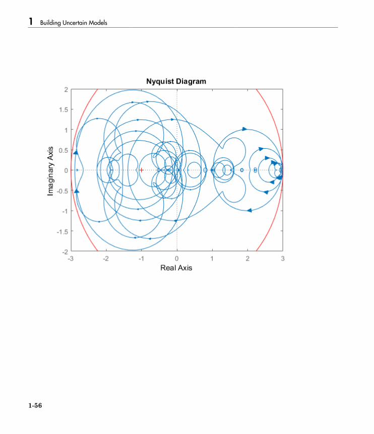
Plot the Nyquist plot of these samples and add a disk of radius 3. Note that the gainbound is satisfied and that the Nyquist plots are all circles, indicative of 1st ordersystems.
nyquist(delS)
hold on;
theta = linspace(-pi,pi);
plot(del.Bound*exp(sqrt(-1)*theta),'r');
hold off;

Generate Samples of Uncertain Systems
1-55
Change SampleStateDimension to 4, and repeat entire procedure. The Nyquist plotssatisfy the gain bound and as expected are more complex than the circles found in the1st-order sampling.
del.SampleStateDimension = 4;
delS = usample(del,30);
nyquist(delS)
hold on;
theta = linspace(-pi,pi);
plot(del.Bound*exp(sqrt(-1)*theta),'r');
hold off;
1 Building Uncertain Models
1-56
Substitution by usubs
1-57
Substitution by usubs
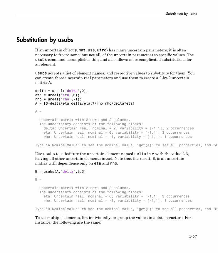
If an uncertain object (umat, uss, ufrd) has many uncertain parameters, it is oftennecessary to freeze some, but not all, of the uncertain parameters to specific values. Theusubs command accomplishes this, and also allows more complicated substitutions foran element.
usubs accepts a list of element names, and respective values to substitute for them. Youcan create three uncertain real parameters and use them to create a 2-by-2 uncertainmatrix A.
delta = ureal('delta',2);
eta = ureal('eta',6);
rho = ureal('rho',-1);
A = [3+delta+eta delta/eta;7+rho rho+delta*eta]
A =
Uncertain matrix with 2 rows and 2 columns.
The uncertainty consists of the following blocks:
delta: Uncertain real, nominal = 2, variability = [-1,1], 2 occurrences
eta: Uncertain real, nominal = 6, variability = [-1,1], 3 occurrences
rho: Uncertain real, nominal = -1, variability = [-1,1], 1 occurrences
Type "A.NominalValue" to see the nominal value, "get(A)" to see all properties, and "A.Uncertainty" to interact with the uncertain elements.
Use usubs to substitute the uncertain element named delta in A with the value 2.3,leaving all other uncertain elements intact. Note that the result, B, is an uncertainmatrix with dependence only on eta and rho.
B = usubs(A,'delta',2.3)
B =
Uncertain matrix with 2 rows and 2 columns.
The uncertainty consists of the following blocks:
eta: Uncertain real, nominal = 6, variability = [-1,1], 3 occurrences
rho: Uncertain real, nominal = -1, variability = [-1,1], 1 occurrences
Type "B.NominalValue" to see the nominal value, "get(B)" to see all properties, and "B.Uncertainty" to interact with the uncertain elements.
To set multiple elements, list individually, or group the values in a data structure. Forinstance, the following are the same.
1 Building Uncertain Models
1-58
B1 = usubs(A,'delta',2.3,'eta',A.Uncertainty.rho);
S.delta = 2.3;
S.eta = A.Uncertainty.rho;
B2 = usubs(A,S);
In each case, delta is replaced by 2.3, and eta is replaced by A.Uncertainty.rho.
Any superfluous substitution requests are ignored. Hence, the following returns anuncertain model that is the same as A.
B4 = usubs(A,'fred',5);
Specifying the Substitution with Structures
An alternative syntax for usubs is to specify the substituted values in a structure, whosefieldnames are the names of the elements being substituted with values.
Create a structure NV with 2 fields, delta and eta. Set the values of these fields to bethe desired substituted values. Then perform the substitution with usubs.
NV.delta = 2.3;
NV.eta = A.Uncertainty.rho;
B6 = usubs(A,NV);
Here, B6 is the same as B1 and B2 above. Again, any superfluous fields are ignored.Therefore, adding an additional field gamma to NV, and substituting does not alter theresult.
NV.gamma = 0;
B7 = usubs(A,NV);
Here, B7 is the same as B6.
The commands wcgain, robuststab and usample all return substitutable values inthis structure format. More discussion can be found in “Create Arrays with usubs” onpage 1-68.
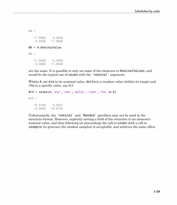
Nominal and Random Values
If the replacement value is the (partial and case-independent) string 'Nominal', thenthe listed element are replaced with their nominal values. Therefore
B8 = usubs(A,fieldnames(A.Uncertainty),'nom')
Substitution by usubs
1-59
B8 =
11.0000 0.3333
6.0000 11.0000
B9 = A.NominalValue
B9 =
11.0000 0.3333
6.0000 11.0000
are the same. It is possible to only set some of the elements to NominalValues, andwould be the typical use of usubs with the 'nominal' argument.
Within A, set eta to its nominal value, delta to a random value (within its range) andrho to a specific value, say 6.5
B10 = usubs(A,'eta','nom','delta','rand','rho',6.5)
B10 =
10.5183 0.2531
13.5000 15.6100
Unfortunately, the 'nominal' and 'Random' specifiers may not be used in thestructure format. However, explicitly setting a field of the structure to an element'snominal value, and then following (or preceeding) the call to usubs with a call tousample (to generate the random samples) is acceptable, and achieves the same effect.
1 Building Uncertain Models
1-60
Array Management for Uncertain Objects
All of the uncertain system classes (uss, ufrd) may be multidimensional arrays.This is intended to provide the same functionality as the LTI-arrays of the ControlSystem Toolbox software. The command size returns a row vector with the sizes of alldimensions.
The first two dimensions correspond to the outputs and inputs of the system. Anydimensions beyond are referred to as the array dimensions. Hence, if szM = size(M),then szM(3:end) are sizes of the array dimensions of M.
For these types of objects, it is clear that the first two dimensions (system output andinput) are interpreted differently from the 3rd, 4th, 5th and higher dimensions (whichoften model parametrized variability in the system input/output behavior).
umat objects are treated in the same manner. The first two dimensions are the rows andcolumns of the uncertain matrix. Any dimensions beyond are the array dimensions.

Reference Into Arrays
1-61
Reference Into Arrays
Suppose M is a umat, uss or ufrd, and that Yidx and Uidx are vectors of integers. Then
M(Yidx,Uidx)
selects the outputs (rows) referred to by Yidx and the inputs (columns) referred to byUidx, preserving all of the array dimensions. For example, if size(M) equals [4 5 3 67], then (for example) the size of M([4 2],[1 2 4]) is [2 3 3 6 7].
If size(M,1)==1 or size(M,2)==1, then single indexing on the inputs or outputs(rows or columns) is allowed. If Sidx is a vector of integers, then M(Sidx) selects thecorresponding elements. All array dimensions are preserved.
If there are K array dimensions, and idx1, idx2, ..., idxK are vectors of integers,then
G = M(Yidx,Uidx,idx1,idx2,...,idxK)
selects the outputs and inputs referred to by Yidx and Uidx, respectively, and selectsfrom each array dimension the “slices” referred to by the idx1, idx2,..., idxKindex vectors. Consequently, size(G,1) equals length(Yidx), size(G,2)equals length(Uidx), size(G,3) equals length(idx1), size(G,4) equalslength(idx2), and size(G,K+2) equals length(idxK).
If M has K array dimensions, and less than K index vectors are used in doing the arrayreferencing, then the MATLAB convention for single indexing is followed. For instance,suppose size(M) equals [3 4 6 5 7 4]. The expression
G = M([1 3],[1 4],[2 3 4],[5 3 1],[8 10 12 2 4 20 18])
is valid. The result has size(G) equals [2 2 3 3 7] . The last index vector [8 10 122 4 20 18] is used to reference into the 7-by-4 array, preserving the order dictated byMATLAB single indexing (e.g., the 10th element of a 7-by-4 array is the element in the(3,2) position in the array).
Note that if M has either one output (row) or one input (column), and M has arraydimensions, then it is not allowable to combine single indexing in the output/inputdimensions along with indexing in the array dimensions. This will result in an ambiguityin how to interpret the second index vector in the expression (i.e., “does it correspond tothe input/output reference, or does it correspond to the first array dimension?”).
1 Building Uncertain Models
1-62
Create Arrays with stack and cat Functions
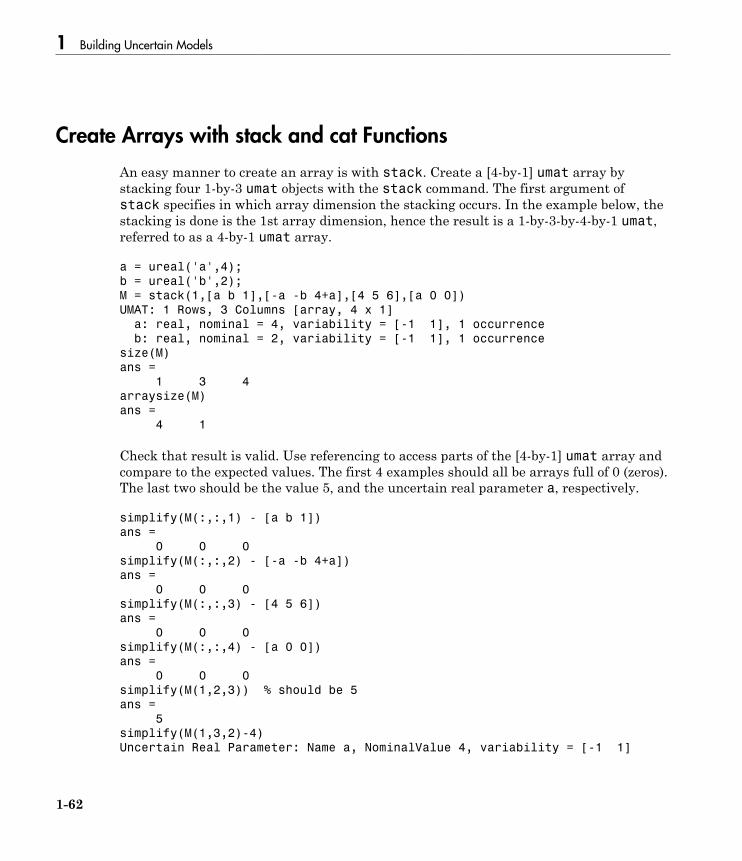
An easy manner to create an array is with stack. Create a [4-by-1] umat array bystacking four 1-by-3 umat objects with the stack command. The first argument ofstack specifies in which array dimension the stacking occurs. In the example below, thestacking is done is the 1st array dimension, hence the result is a 1-by-3-by-4-by-1 umat,referred to as a 4-by-1 umat array.
a = ureal('a',4);
b = ureal('b',2);
M = stack(1,[a b 1],[-a -b 4+a],[4 5 6],[a 0 0])
UMAT: 1 Rows, 3 Columns [array, 4 x 1]
a: real, nominal = 4, variability = [-1 1], 1 occurrence
b: real, nominal = 2, variability = [-1 1], 1 occurrence
size(M)
ans =
1 3 4
arraysize(M)
ans =
4 1
Check that result is valid. Use referencing to access parts of the [4-by-1] umat array andcompare to the expected values. The first 4 examples should all be arrays full of 0 (zeros).The last two should be the value 5, and the uncertain real parameter a, respectively.
simplify(M(:,:,1) - [a b 1])
ans =
0 0 0
simplify(M(:,:,2) - [-a -b 4+a])
ans =
0 0 0
simplify(M(:,:,3) - [4 5 6])
ans =
0 0 0
simplify(M(:,:,4) - [a 0 0])
ans =
0 0 0
simplify(M(1,2,3)) % should be 5
ans =
5
simplify(M(1,3,2)-4)
Uncertain Real Parameter: Name a, NominalValue 4, variability = [-1 1]
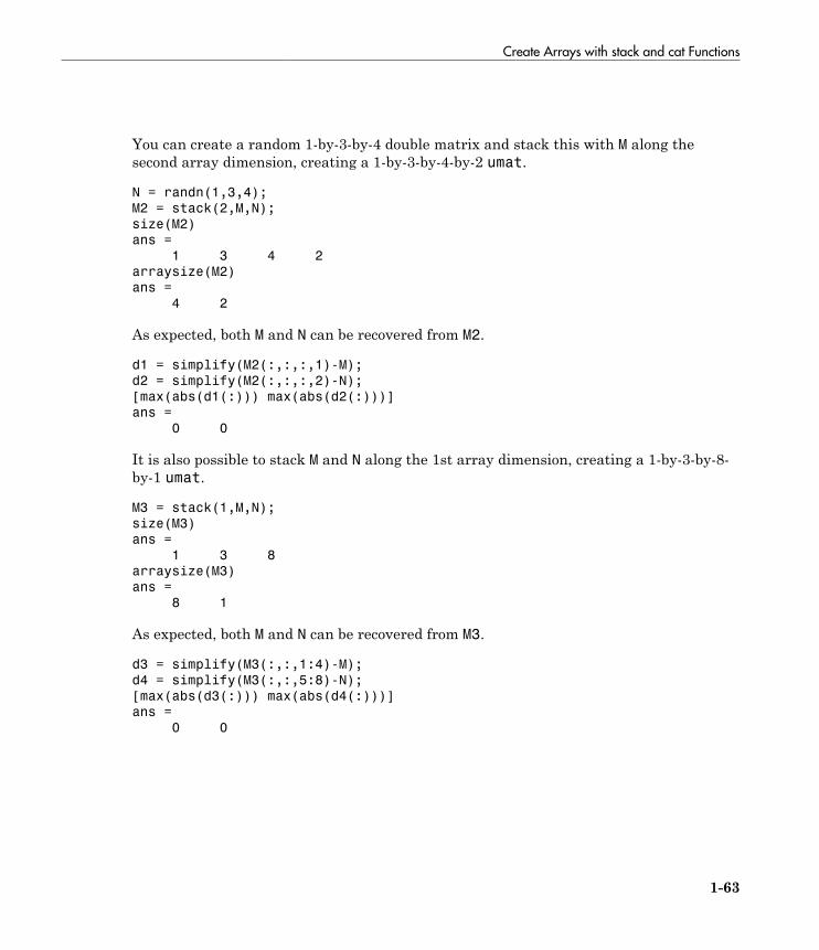
Create Arrays with stack and cat Functions
1-63
You can create a random 1-by-3-by-4 double matrix and stack this with M along thesecond array dimension, creating a 1-by-3-by-4-by-2 umat.
N = randn(1,3,4);
M2 = stack(2,M,N);
size(M2)
ans =
1 3 4 2
arraysize(M2)
ans =
4 2
As expected, both M and N can be recovered from M2.
d1 = simplify(M2(:,:,:,1)-M);
d2 = simplify(M2(:,:,:,2)-N);
[max(abs(d1(:))) max(abs(d2(:)))]
ans =
0 0
It is also possible to stack M and N along the 1st array dimension, creating a 1-by-3-by-8-by-1 umat.
M3 = stack(1,M,N);
size(M3)
ans =
1 3 8
arraysize(M3)
ans =
8 1
As expected, both M and N can be recovered from M3.
d3 = simplify(M3(:,:,1:4)-M);
d4 = simplify(M3(:,:,5:8)-N);
[max(abs(d3(:))) max(abs(d4(:)))]
ans =
0 0

1 Building Uncertain Models
1-64
Create Arrays by Assignment
Arrays can be created by direct assignment. As with other MATLAB classes, there is noneed to preallocate the variable first. Simply assign elements – all resizing is performedautomatically.
For instance, an equivalent construction to
a = ureal('a',4);
b = ureal('b',2);
M = stack(1,[a b 1],[-a -b 4+a],[4 5 6],[a 0 0]);
is
Mequiv(1,1,1) = a;
Mequiv(1,2,1) = b;
Mequiv(1,3,1) = 1;
Mequiv(1,:,4) = [a 0 0];
Mequiv(1,:,2:3) = stack(1,[-a -b 4+a],[4 5 6]);
The easiest manner for you to verify that the results are the same is to subtract andsimplify,
d5 = simplify(M-Mequiv);
max(abs(d5(:)))
ans =
0

Binary Operations with Arrays
1-65
Binary Operations with Arrays
Most operations simply cycle through the array dimensions, doing pointwise operations.Assume A and B are umat (or uss, or ufrd) arrays with identical array dimensions (slot3 and beyond). The operation C = fcn(A,B) is equivalent to looping on k1, k2, ...,setting
C(:,:,k1,k2,...) = fcn(A(:,:,k1,k2,...),B(:,:,k1,k2,...))
The result C has the same array dimensions as A and B. The user is required to managethe extra dimensions (i.e., keep track of what they mean). Methods such as permute,squeeze and reshape are included to facilitate this management.
In general, any binary operation requires that the extra-dimensions are compatible. Theumat, uss and ufrd objects allow for slightly more flexible interpretation of this. Forillustrative purposes, consider a binary operation involving variables A and B. Supposethe array dimensions of A are n nl
A1 ¥ ¥… and that the array dimensions of B are
m mlB
1 ¥ ¥… . By MATLAB convention, the infinite number of singleton (i.e., 1) trailingdimensions are not listed. The compatibility of the extra dimensions is determinedby the following rule: If lA = lB, then pad the shorter dimension list with trailing 1's.Now compare the extra dimensions: In the k-th dimension, it must be that one of 3conditions hold: nk = mk, or nk = 1, or mk = 1. In other words, non-singleton dimensionsmust exactly match (so that the pointwise operation can be executed), and singletondimensions match with anything, implicitly through a repmat.
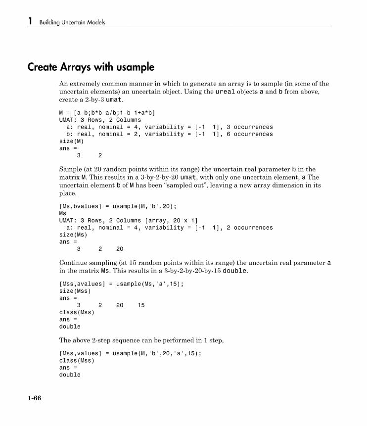
1 Building Uncertain Models
1-66
Create Arrays with usample
An extremely common manner in which to generate an array is to sample (in some of theuncertain elements) an uncertain object. Using the ureal objects a and b from above,create a 2-by-3 umat.
M = [a b;b*b a/b;1-b 1+a*b]
UMAT: 3 Rows, 2 Columns
a: real, nominal = 4, variability = [-1 1], 3 occurrences
b: real, nominal = 2, variability = [-1 1], 6 occurrences
size(M)
ans =
3 2
Sample (at 20 random points within its range) the uncertain real parameter b in thematrix M. This results in a 3-by-2-by-20 umat, with only one uncertain element, a Theuncertain element b of M has been “sampled out”, leaving a new array dimension in itsplace.
[Ms,bvalues] = usample(M,'b',20);
Ms
UMAT: 3 Rows, 2 Columns [array, 20 x 1]
a: real, nominal = 4, variability = [-1 1], 2 occurrences
size(Ms)
ans =
3 2 20
Continue sampling (at 15 random points within its range) the uncertain real parameter ain the matrix Ms. This results in a 3-by-2-by-20-by-15 double.
[Mss,avalues] = usample(Ms,'a',15);
size(Mss)
ans =
3 2 20 15
class(Mss)
ans =
double
The above 2-step sequence can be performed in 1 step,
[Mss,values] = usample(M,'b',20,'a',15);
class(Mss)
ans =
double
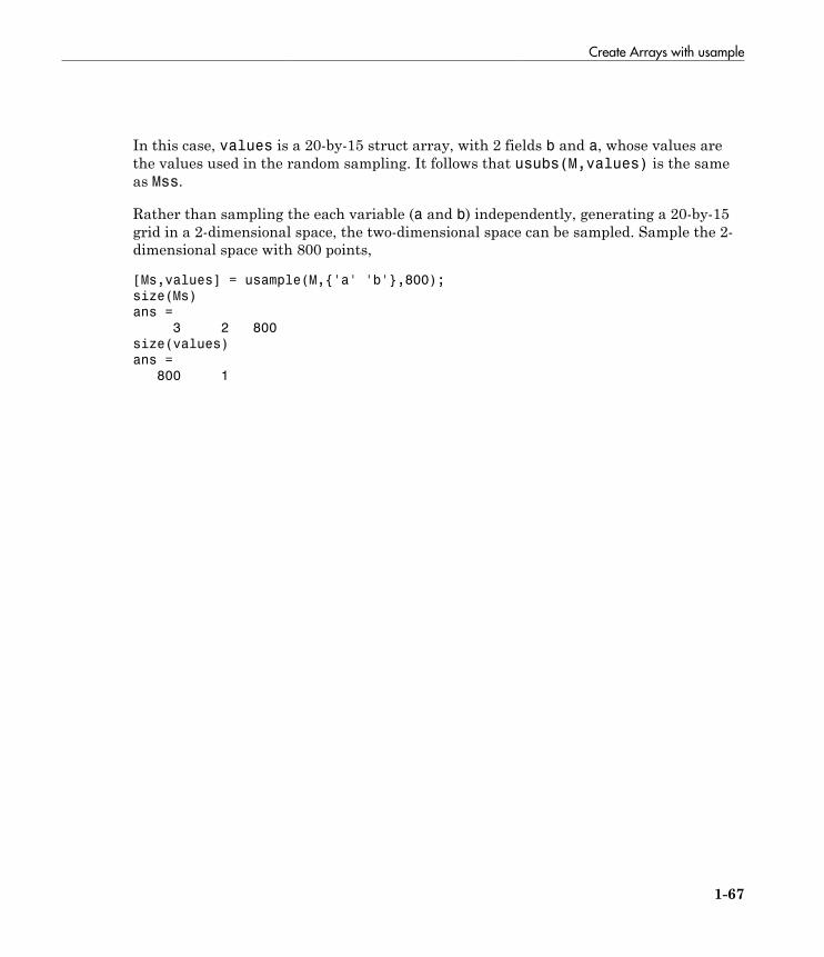
Create Arrays with usample
1-67
In this case, values is a 20-by-15 struct array, with 2 fields b and a, whose values arethe values used in the random sampling. It follows that usubs(M,values) is the sameas Mss.
Rather than sampling the each variable (a and b) independently, generating a 20-by-15grid in a 2-dimensional space, the two-dimensional space can be sampled. Sample the 2-dimensional space with 800 points,
[Ms,values] = usample(M,{'a' 'b'},800);
size(Ms)
ans =
3 2 800
size(values)
ans =
800 1
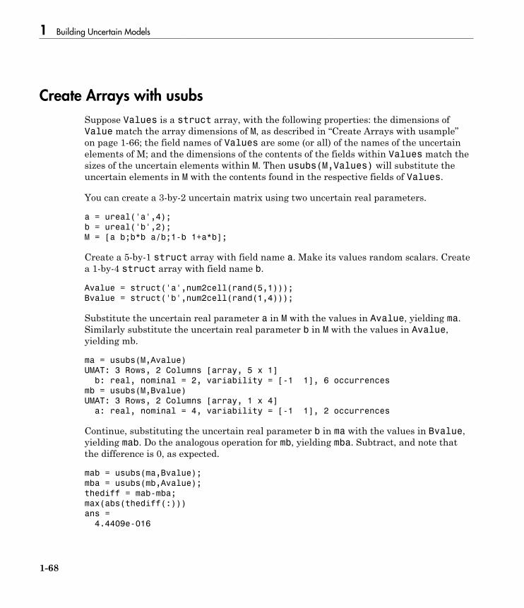
1 Building Uncertain Models
1-68
Create Arrays with usubs
Suppose Values is a struct array, with the following properties: the dimensions ofValue match the array dimensions of M, as described in “Create Arrays with usample”on page 1-66; the field names of Values are some (or all) of the names of the uncertainelements of M; and the dimensions of the contents of the fields within Values match thesizes of the uncertain elements within M. Then usubs(M,Values) will substitute theuncertain elements in M with the contents found in the respective fields of Values.
You can create a 3-by-2 uncertain matrix using two uncertain real parameters.
a = ureal('a',4);
b = ureal('b',2);
M = [a b;b*b a/b;1-b 1+a*b];
Create a 5-by-1 struct array with field name a. Make its values random scalars. Createa 1-by-4 struct array with field name b.
Avalue = struct('a',num2cell(rand(5,1)));
Bvalue = struct('b',num2cell(rand(1,4)));
Substitute the uncertain real parameter a in M with the values in Avalue, yielding ma.Similarly substitute the uncertain real parameter b in M with the values in Avalue,yielding mb.
ma = usubs(M,Avalue)
UMAT: 3 Rows, 2 Columns [array, 5 x 1]
b: real, nominal = 2, variability = [-1 1], 6 occurrences
mb = usubs(M,Bvalue)
UMAT: 3 Rows, 2 Columns [array, 1 x 4]
a: real, nominal = 4, variability = [-1 1], 2 occurrences
Continue, substituting the uncertain real parameter b in ma with the values in Bvalue,yielding mab. Do the analogous operation for mb, yielding mba. Subtract, and note thatthe difference is 0, as expected.
mab = usubs(ma,Bvalue);
mba = usubs(mb,Avalue);
thediff = mab-mba;
max(abs(thediff(:)))
ans =
4.4409e-016
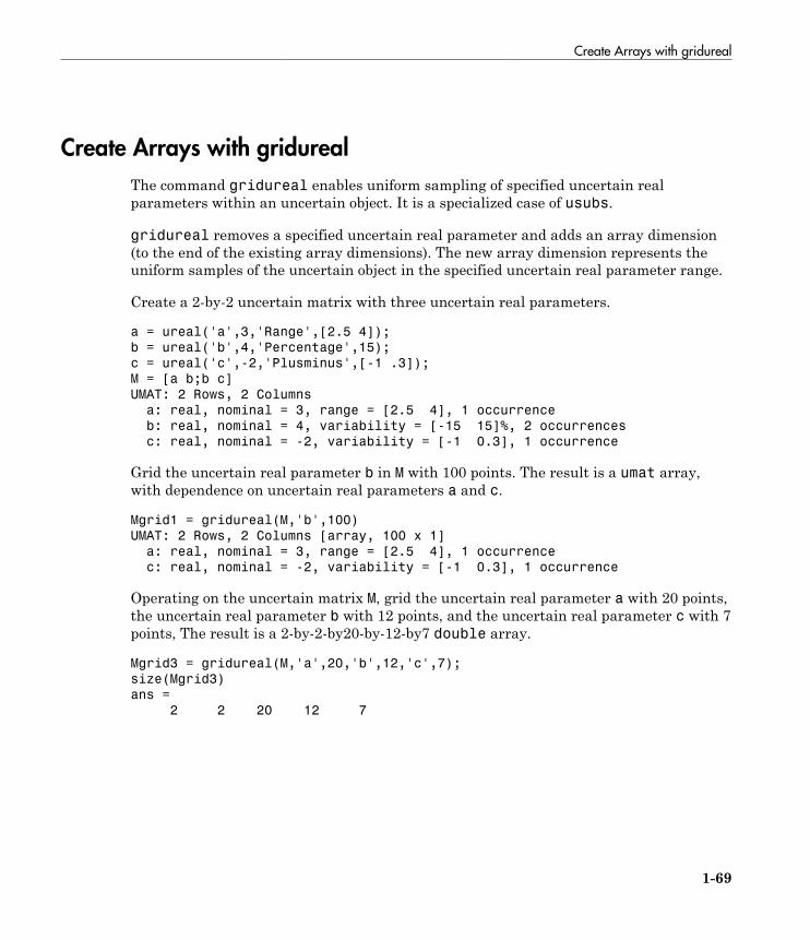
Create Arrays with gridureal
1-69
Create Arrays with gridureal
The command gridureal enables uniform sampling of specified uncertain realparameters within an uncertain object. It is a specialized case of usubs.
gridureal removes a specified uncertain real parameter and adds an array dimension(to the end of the existing array dimensions). The new array dimension represents theuniform samples of the uncertain object in the specified uncertain real parameter range.
Create a 2-by-2 uncertain matrix with three uncertain real parameters.
a = ureal('a',3,'Range',[2.5 4]);
b = ureal('b',4,'Percentage',15);
c = ureal('c',-2,'Plusminus',[-1 .3]);
M = [a b;b c]
UMAT: 2 Rows, 2 Columns
a: real, nominal = 3, range = [2.5 4], 1 occurrence
b: real, nominal = 4, variability = [-15 15]%, 2 occurrences
c: real, nominal = -2, variability = [-1 0.3], 1 occurrence
Grid the uncertain real parameter b in M with 100 points. The result is a umat array,with dependence on uncertain real parameters a and c.
Mgrid1 = gridureal(M,'b',100)
UMAT: 2 Rows, 2 Columns [array, 100 x 1]
a: real, nominal = 3, range = [2.5 4], 1 occurrence
c: real, nominal = -2, variability = [-1 0.3], 1 occurrence
Operating on the uncertain matrix M, grid the uncertain real parameter a with 20 points,the uncertain real parameter b with 12 points, and the uncertain real parameter c with 7points, The result is a 2-by-2-by20-by-12-by7 double array.
Mgrid3 = gridureal(M,'a',20,'b',12,'c',7);
size(Mgrid3)
ans =
2 2 20 12 7
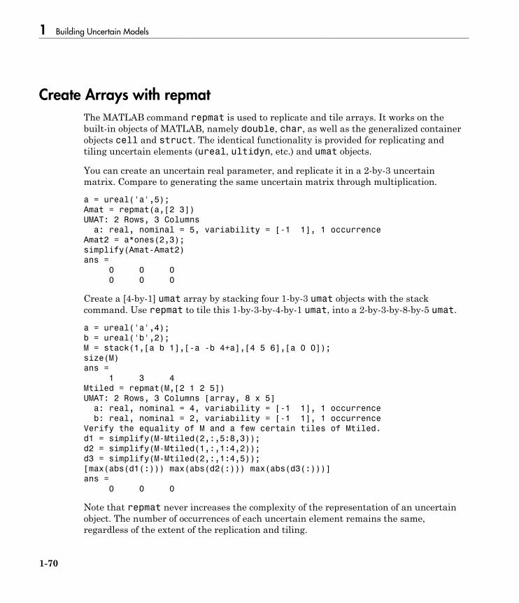
1 Building Uncertain Models
1-70
Create Arrays with repmatThe MATLAB command repmat is used to replicate and tile arrays. It works on thebuilt-in objects of MATLAB, namely double, char, as well as the generalized containerobjects cell and struct. The identical functionality is provided for replicating andtiling uncertain elements (ureal, ultidyn, etc.) and umat objects.
You can create an uncertain real parameter, and replicate it in a 2-by-3 uncertainmatrix. Compare to generating the same uncertain matrix through multiplication.
a = ureal('a',5);
Amat = repmat(a,[2 3])
UMAT: 2 Rows, 3 Columns
a: real, nominal = 5, variability = [-1 1], 1 occurrence
Amat2 = a*ones(2,3);
simplify(Amat-Amat2)
ans =
0 0 0
0 0 0
Create a [4-by-1] umat array by stacking four 1-by-3 umat objects with the stackcommand. Use repmat to tile this 1-by-3-by-4-by-1 umat, into a 2-by-3-by-8-by-5 umat.
a = ureal('a',4);
b = ureal('b',2);
M = stack(1,[a b 1],[-a -b 4+a],[4 5 6],[a 0 0]);
size(M)
ans =
1 3 4
Mtiled = repmat(M,[2 1 2 5])
UMAT: 2 Rows, 3 Columns [array, 8 x 5]
a: real, nominal = 4, variability = [-1 1], 1 occurrence
b: real, nominal = 2, variability = [-1 1], 1 occurrence
Verify the equality of M and a few certain tiles of Mtiled.
d1 = simplify(M-Mtiled(2,:,5:8,3));
d2 = simplify(M-Mtiled(1,:,1:4,2));
d3 = simplify(M-Mtiled(2,:,1:4,5));
[max(abs(d1(:))) max(abs(d2(:))) max(abs(d3(:)))]
ans =
0 0 0
Note that repmat never increases the complexity of the representation of an uncertainobject. The number of occurrences of each uncertain element remains the same,regardless of the extent of the replication and tiling.

Create Arrays with repsys
1-71
Create Arrays with repsys
Replicating and tiling uncertain state-space systems (uss, and uncertain frequencyresponse data (ufrd) is done with repsys. The syntax and behavior are the same as themanner in which repmat is used to replicate and tile matrices. The syntax and behaviorof repsys for uss and ufrd objects are the same as the traditional repsys whichoperates on ss and frd objects. Just as in those cases, the uncertain version of repsysalso allows for diagonal tiling.
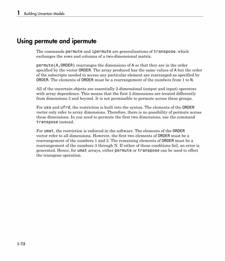
1 Building Uncertain Models
1-72
Using permute and ipermute
The commands permute and ipermute are generalizations of transpose, whichexchanges the rows and columns of a two-dimensional matrix.
permute(A,ORDER) rearranges the dimensions of A so that they are in the orderspecified by the vector ORDER. The array produced has the same values of A but the orderof the subscripts needed to access any particular element are rearranged as specified byORDER. The elements of ORDER must be a rearrangement of the numbers from 1 to N.
All of the uncertain objects are essentially 2-dimensional (output and input) operatorswith array dependence. This means that the first 2 dimensions are treated differentlyfrom dimensions 3 and beyond. It is not permissible to permute across these groups.
For uss and ufrd, the restriction is built into the syntax. The elements of the ORDERvector only refer to array dimensions. Therefore, there is no possibility of permute acrossthese dimensions. In you need to permute the first two dimensions, use the commandtranspose instead.
For umat, the restriction is enforced in the software. The elements of the ORDERvector refer to all dimensions. However, the first two elements of ORDER must be arearrangement of the numbers 1 and 2. The remaining elements of ORDER must be arearrangement of the numbers 3 through N. If either of those conditions fail, an error isgenerated. Hence, for umat arrays, either permute or transpose can be used to effectthe transpose operation.

Decomposing Uncertain Objects
1-73
Decomposing Uncertain Objects
Each uncertain object (umat, uss, ufrd) is a generalized feedback connection (lft) of anot-uncertain object (e.g., double, ss, frd) with a diagonal augmentation of uncertainelements (ureal, ultidyn, ucomplex, ucomplexm, udyn). In robust control jargon, ifthe uncertain elements are normalized, this decomposition is often called “the M/D form.”
The purpose of the uncertain objects (ureal, ultidyn, umat, uss, etc.) is tohide this underlying decomposition, and allow the user to focus on modeling andanalyzing uncertain systems, rather than the details of correctly propagating the M/Drepresentation in manipulations. Nevertheless, advanced users may want access to thefamiliar M/D form. The command lftdata accomplishes this decomposition.
Since ureal, ucomplex and ucomplexm do not have their NominalValue necessarily atzero, and in the case of ureal objects, are not symmetric about the NominalValue, somedetails are required in describing the decomposition.
Normalizing Functions for Uncertain Elements
Associated with each uncertain element is a normalizing function. The normalizingfunction maps the uncertain element into a normalized uncertain element.
If ρ is an uncertain real parameter, with range [L R] and nominal value N, then thenormalizing function F is
FA B
C Dr
r
r( ) =
+
+
with the property that for all ρ satisfying L ≤ ρ ≤ R, it follows that –1 ≤ F(ρ) ≤ 1,moreover, F(L) = –1, F(N) = 0, and F(R) = 1. If the nominal value is centered in the range,then it is easy to conclude that
AR L
R L
BR L
C
D
=
+
-
=
-
=
=
2
1
0.
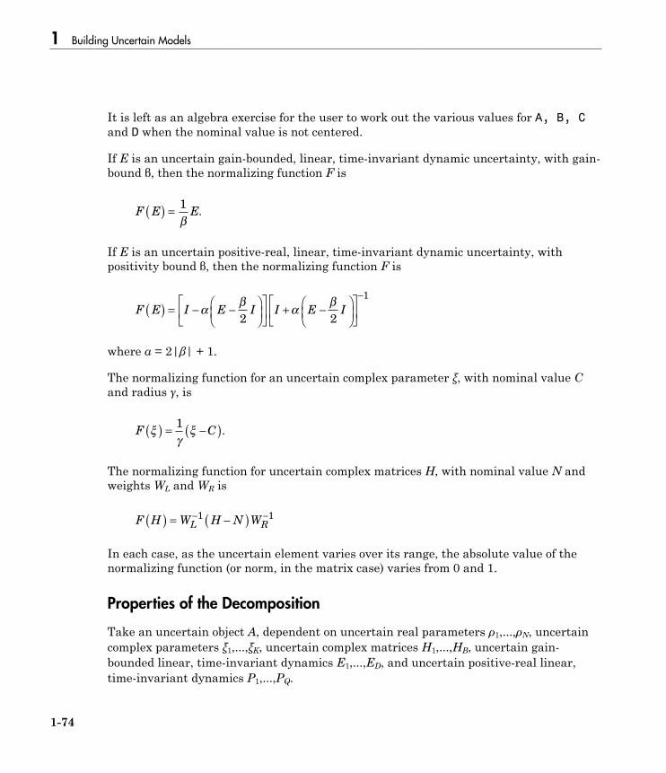
1 Building Uncertain Models
1-74
It is left as an algebra exercise for the user to work out the various values for A, B, Cand D when the nominal value is not centered.
If E is an uncertain gain-bounded, linear, time-invariant dynamic uncertainty, with gain-bound β, then the normalizing function F is
F E E( ) =1
b.
If E is an uncertain positive-real, linear, time-invariant dynamic uncertainty, withpositivity bound β, then the normalizing function F is
F E I E I I E I( ) = - -ÊËÁ
ˆ¯
È
ÎÍ
˘
˚˙ + -Ê
ËÁˆ¯
È
ÎÍ
˘
˚˙
-
ab
ab
2 2
1
where α = 2|β| + 1.
The normalizing function for an uncertain complex parameter ξ, with nominal value Cand radius γ, is
F Cxg
x( ) = -( )1
.
The normalizing function for uncertain complex matrices H, with nominal value N andweights WL and WR is
F H W H N WL R( ) = -( )- -1 1
In each case, as the uncertain element varies over its range, the absolute value of thenormalizing function (or norm, in the matrix case) varies from 0 and 1.
Properties of the Decomposition
Take an uncertain object A, dependent on uncertain real parameters ρ1,...,ρN, uncertaincomplex parameters ξ1,...,ξK, uncertain complex matrices H1,...,HB, uncertain gain-bounded linear, time-invariant dynamics E1,...,ED, and uncertain positive-real linear,time-invariant dynamics P1,...,PQ.
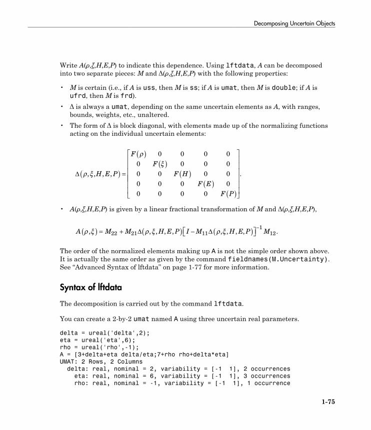
Decomposing Uncertain Objects
1-75
Write A(ρ,ξ,H,E,P) to indicate this dependence. Using lftdata, A can be decomposedinto two separate pieces: M and Δ(ρ,ξ,H,E,P) with the following properties:
• M is certain (i.e., if A is uss, then M is ss; if A is umat, then M is double; if A isufrd, then M is frd).
• Δ is always a umat, depending on the same uncertain elements as A, with ranges,bounds, weights, etc., unaltered.
• The form of Δ is block diagonal, with elements made up of the normalizing functionsacting on the individual uncertain elements:
D r x
r
x
, , , ,H E P
F
F
F H
F E
F P
( ) =
( )( )
( )( )
( )
È
Î
ÍÍÍ
0 0 0 0
0 0 0 0
0 0 0 0
0 0 0 0
0 0 0 0
ÍÍÍÍ
˘
˚
˙˙˙˙˙˙
.
• A(ρ,ξ,H,E,P) is given by a linear fractional transformation of M and Δ(ρ,ξ,H,E,P),
A M M H E P I M H E P Mr x r x r x, , , , , , , , , .( ) = + ( ) - ( )ÈÎ ˘-
22 21 11
1
12D D
The order of the normalized elements making up A is not the simple order shown above.It is actually the same order as given by the command fieldnames(M.Uncertainty).See “Advanced Syntax of lftdata” on page 1-77 for more information.
Syntax of lftdata
The decomposition is carried out by the command lftdata.
You can create a 2-by-2 umat named A using three uncertain real parameters.
delta = ureal('delta',2);
eta = ureal('eta',6);
rho = ureal('rho',-1);
A = [3+delta+eta delta/eta;7+rho rho+delta*eta]
UMAT: 2 Rows, 2 Columns
delta: real, nominal = 2, variability = [-1 1], 2 occurrences
eta: real, nominal = 6, variability = [-1 1], 3 occurrences
rho: real, nominal = -1, variability = [-1 1], 1 occurrence
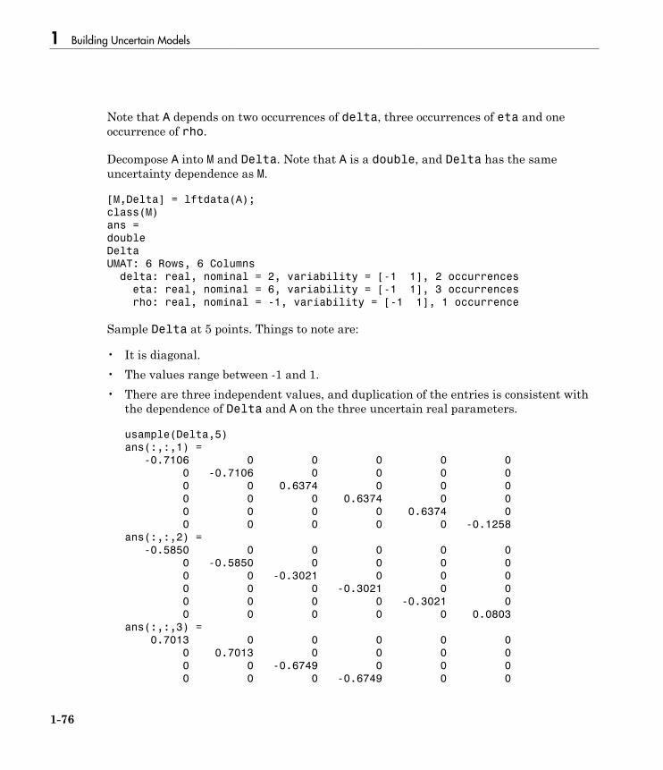
1 Building Uncertain Models
1-76
Note that A depends on two occurrences of delta, three occurrences of eta and oneoccurrence of rho.
Decompose A into M and Delta. Note that A is a double, and Delta has the sameuncertainty dependence as M.
[M,Delta] = lftdata(A);
class(M)
ans =
double
Delta
UMAT: 6 Rows, 6 Columns
delta: real, nominal = 2, variability = [-1 1], 2 occurrences
eta: real, nominal = 6, variability = [-1 1], 3 occurrences
rho: real, nominal = -1, variability = [-1 1], 1 occurrence
Sample Delta at 5 points. Things to note are:
• It is diagonal.• The values range between -1 and 1.• There are three independent values, and duplication of the entries is consistent with
the dependence of Delta and A on the three uncertain real parameters.
usample(Delta,5)
ans(:,:,1) =
-0.7106 0 0 0 0 0
0 -0.7106 0 0 0 0
0 0 0.6374 0 0 0
0 0 0 0.6374 0 0
0 0 0 0 0.6374 0
0 0 0 0 0 -0.1258
ans(:,:,2) =
-0.5850 0 0 0 0 0
0 -0.5850 0 0 0 0
0 0 -0.3021 0 0 0
0 0 0 -0.3021 0 0
0 0 0 0 -0.3021 0
0 0 0 0 0 0.0803
ans(:,:,3) =
0.7013 0 0 0 0 0
0 0.7013 0 0 0 0
0 0 -0.6749 0 0 0
0 0 0 -0.6749 0 0
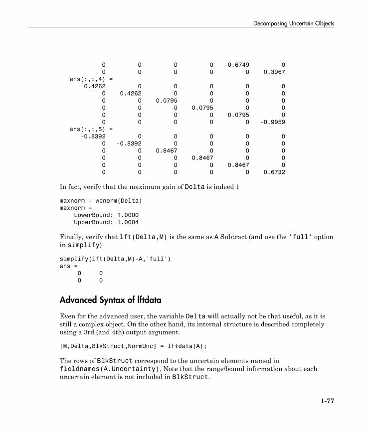
Decomposing Uncertain Objects
1-77
0 0 0 0 -0.6749 0
0 0 0 0 0 0.3967
ans(:,:,4) =
0.4262 0 0 0 0 0
0 0.4262 0 0 0 0
0 0 0.0795 0 0 0
0 0 0 0.0795 0 0
0 0 0 0 0.0795 0
0 0 0 0 0 -0.9959
ans(:,:,5) =
-0.8392 0 0 0 0 0
0 -0.8392 0 0 0 0
0 0 0.8467 0 0 0
0 0 0 0.8467 0 0
0 0 0 0 0.8467 0
0 0 0 0 0 0.6732
In fact, verify that the maximum gain of Delta is indeed 1
maxnorm = wcnorm(Delta)
maxnorm =
LowerBound: 1.0000
UpperBound: 1.0004
Finally, verify that lft(Delta,M) is the same as A Subtract (and use the 'full' optionin simplify)
simplify(lft(Delta,M)-A,'full')
ans =
0 0
0 0
Advanced Syntax of lftdata
Even for the advanced user, the variable Delta will actually not be that useful, as it isstill a complex object. On the other hand, its internal structure is described completelyusing a 3rd (and 4th) output argument.
[M,Delta,BlkStruct,NormUnc] = lftdata(A);
The rows of BlkStruct correspond to the uncertain elements named infieldnames(A.Uncertainty). Note that the range/bound information about eachuncertain element is not included in BlkStruct.
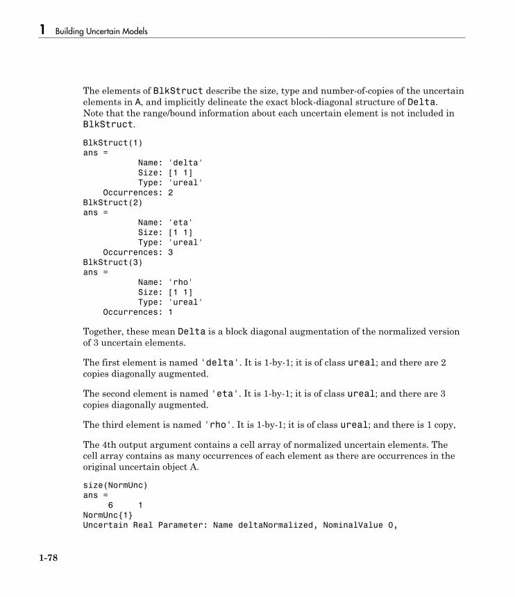
1 Building Uncertain Models
1-78
The elements of BlkStruct describe the size, type and number-of-copies of the uncertainelements in A, and implicitly delineate the exact block-diagonal structure of Delta.Note that the range/bound information about each uncertain element is not included inBlkStruct.
BlkStruct(1)
ans =
Name: 'delta'
Size: [1 1]
Type: 'ureal'
Occurrences: 2
BlkStruct(2)
ans =
Name: 'eta'
Size: [1 1]
Type: 'ureal'
Occurrences: 3
BlkStruct(3)
ans =
Name: 'rho'
Size: [1 1]
Type: 'ureal'
Occurrences: 1
Together, these mean Delta is a block diagonal augmentation of the normalized versionof 3 uncertain elements.
The first element is named 'delta'. It is 1-by-1; it is of class ureal; and there are 2copies diagonally augmented.
The second element is named 'eta'. It is 1-by-1; it is of class ureal; and there are 3copies diagonally augmented.
The third element is named 'rho'. It is 1-by-1; it is of class ureal; and there is 1 copy,
The 4th output argument contains a cell array of normalized uncertain elements. Thecell array contains as many occurrences of each element as there are occurrences in theoriginal uncertain object A.
size(NormUnc)
ans =
6 1
NormUnc{1}
Uncertain Real Parameter: Name deltaNormalized, NominalValue 0,
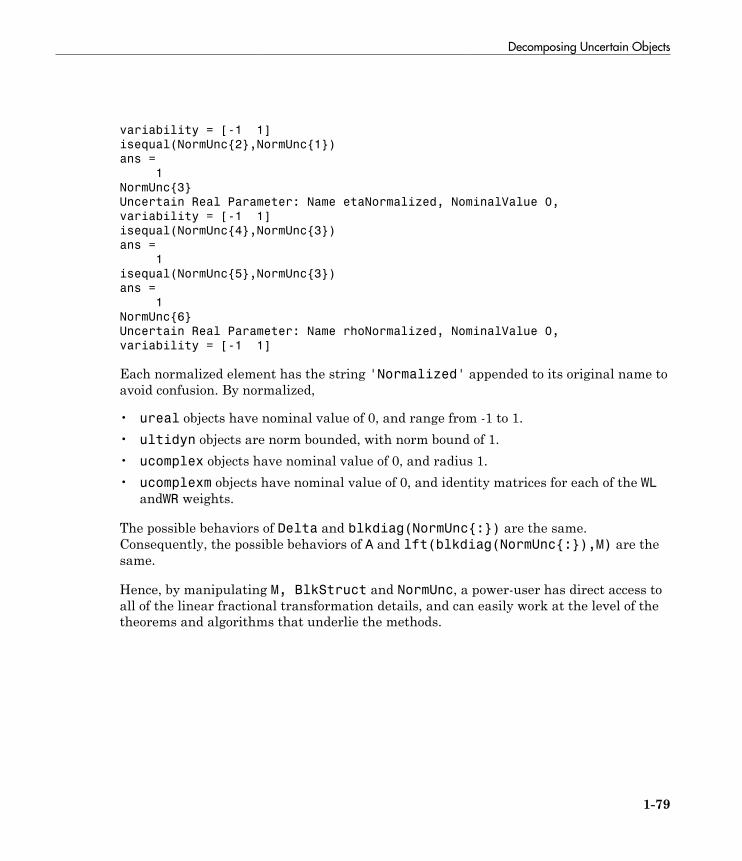
Decomposing Uncertain Objects
1-79
variability = [-1 1]
isequal(NormUnc{2},NormUnc{1})
ans =
1
NormUnc{3}
Uncertain Real Parameter: Name etaNormalized, NominalValue 0,
variability = [-1 1]
isequal(NormUnc{4},NormUnc{3})
ans =
1
isequal(NormUnc{5},NormUnc{3})
ans =
1
NormUnc{6}
Uncertain Real Parameter: Name rhoNormalized, NominalValue 0,
variability = [-1 1]
Each normalized element has the string 'Normalized' appended to its original name toavoid confusion. By normalized,
• ureal objects have nominal value of 0, and range from -1 to 1.• ultidyn objects are norm bounded, with norm bound of 1.• ucomplex objects have nominal value of 0, and radius 1.• ucomplexm objects have nominal value of 0, and identity matrices for each of the WL
andWR weights.
The possible behaviors of Delta and blkdiag(NormUnc{:}) are the same.Consequently, the possible behaviors of A and lft(blkdiag(NormUnc{:}),M) are thesame.
Hence, by manipulating M, BlkStruct and NormUnc, a power-user has direct access toall of the linear fractional transformation details, and can easily work at the level of thetheorems and algorithms that underlie the methods.

2
Generalized Robustness Analysis
• “Generalized Robustness Analysis” on page 2-2• “Robust Stability Margin” on page 2-4• “Robust Performance Margin” on page 2-5• “Worst-Case Gain Measure” on page 2-6
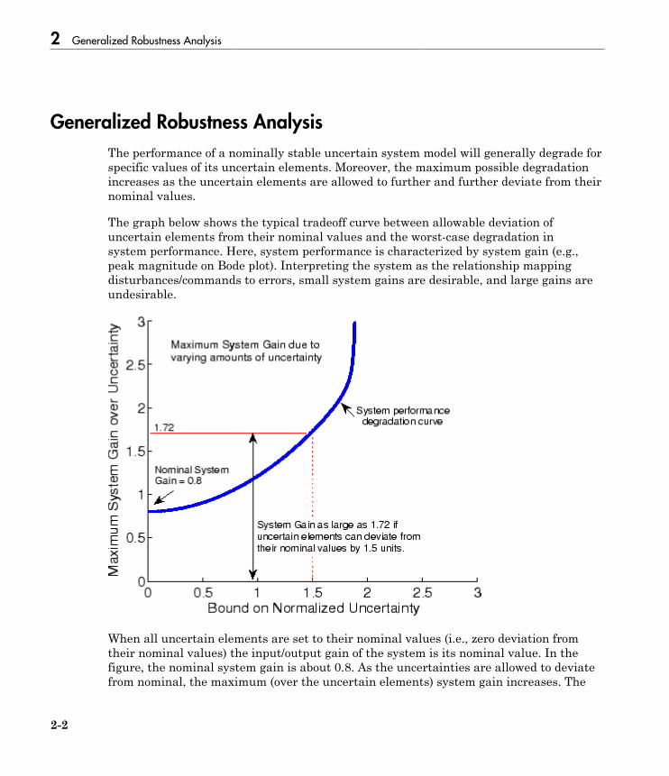
2 Generalized Robustness Analysis
2-2
Generalized Robustness Analysis
The performance of a nominally stable uncertain system model will generally degrade forspecific values of its uncertain elements. Moreover, the maximum possible degradationincreases as the uncertain elements are allowed to further and further deviate from theirnominal values.
The graph below shows the typical tradeoff curve between allowable deviation ofuncertain elements from their nominal values and the worst-case degradation insystem performance. Here, system performance is characterized by system gain (e.g.,peak magnitude on Bode plot). Interpreting the system as the relationship mappingdisturbances/commands to errors, small system gains are desirable, and large gains areundesirable.
When all uncertain elements are set to their nominal values (i.e., zero deviation fromtheir nominal values) the input/output gain of the system is its nominal value. In thefigure, the nominal system gain is about 0.8. As the uncertainties are allowed to deviatefrom nominal, the maximum (over the uncertain elements) system gain increases. The
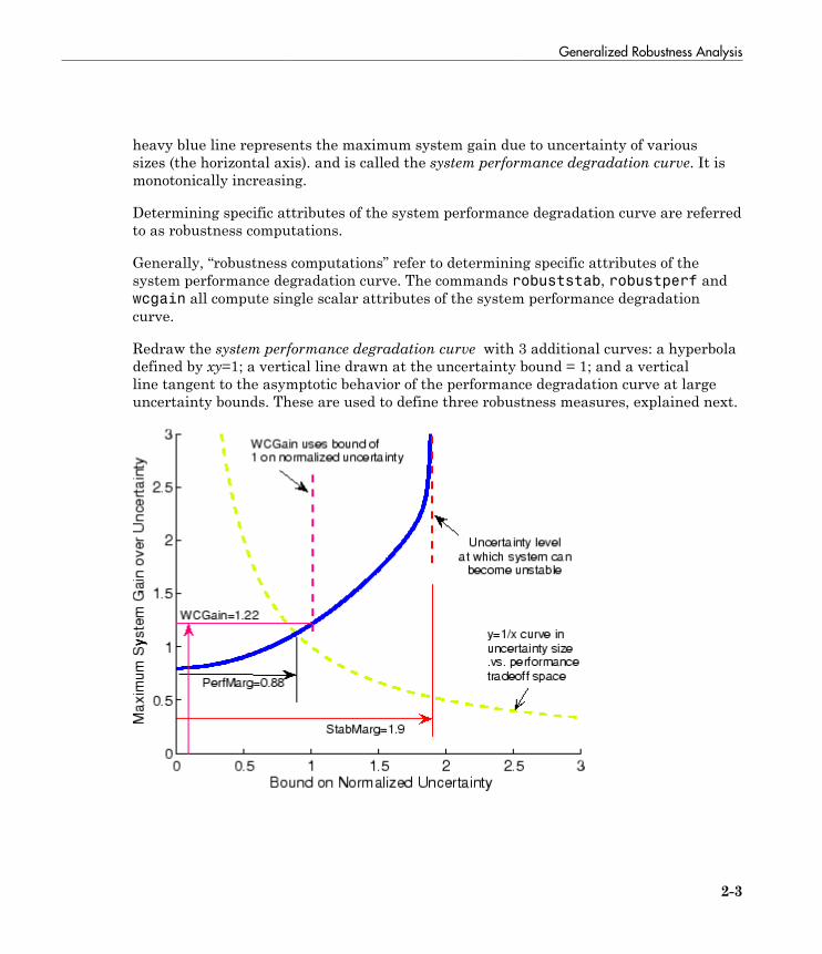
Generalized Robustness Analysis
2-3
heavy blue line represents the maximum system gain due to uncertainty of varioussizes (the horizontal axis). and is called the system performance degradation curve. It ismonotonically increasing.
Determining specific attributes of the system performance degradation curve are referredto as robustness computations.
Generally, “robustness computations” refer to determining specific attributes of thesystem performance degradation curve. The commands robuststab, robustperf andwcgain all compute single scalar attributes of the system performance degradationcurve.
Redraw the system performance degradation curve with 3 additional curves: a hyperboladefined by xy=1; a vertical line drawn at the uncertainty bound = 1; and a verticalline tangent to the asymptotic behavior of the performance degradation curve at largeuncertainty bounds. These are used to define three robustness measures, explained next.
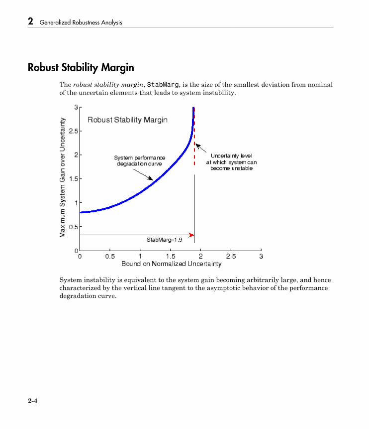
2 Generalized Robustness Analysis
2-4
Robust Stability Margin
The robust stability margin, StabMarg, is the size of the smallest deviation from nominalof the uncertain elements that leads to system instability.
System instability is equivalent to the system gain becoming arbitrarily large, and hencecharacterized by the vertical line tangent to the asymptotic behavior of the performancedegradation curve.
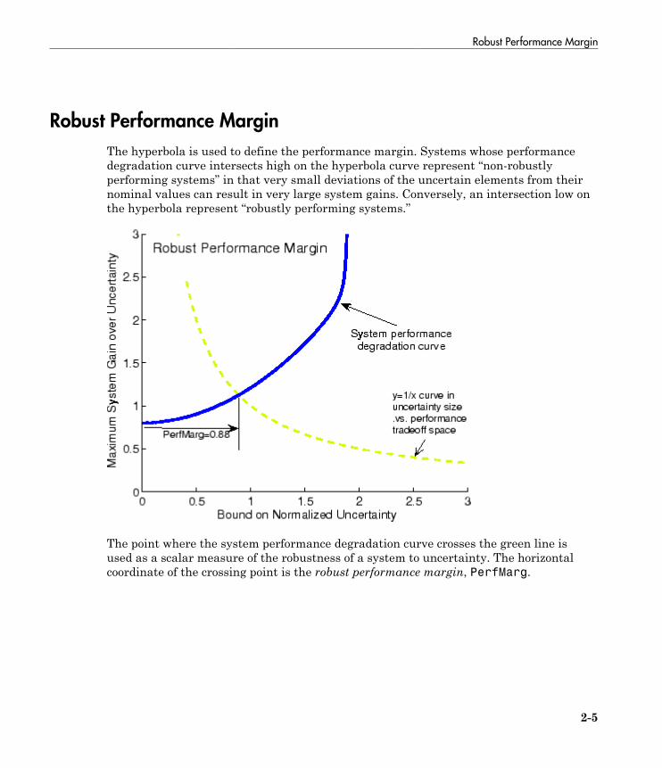
Robust Performance Margin
2-5
Robust Performance Margin
The hyperbola is used to define the performance margin. Systems whose performancedegradation curve intersects high on the hyperbola curve represent “non-robustlyperforming systems” in that very small deviations of the uncertain elements from theirnominal values can result in very large system gains. Conversely, an intersection low onthe hyperbola represent “robustly performing systems.”
The point where the system performance degradation curve crosses the green line isused as a scalar measure of the robustness of a system to uncertainty. The horizontalcoordinate of the crossing point is the robust performance margin, PerfMarg.
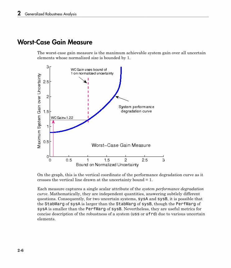
2 Generalized Robustness Analysis
2-6
Worst-Case Gain Measure
The worst-case gain measure is the maximum achievable system gain over all uncertainelements whose normalized size is bounded by 1.
On the graph, this is the vertical coordinate of the performance degradation curve as itcrosses the vertical line drawn at the uncertainty bound = 1.
Each measure captures a single scalar attribute of the system performance degradationcurve. Mathematically, they are independent quantities, answering subtlely differentquestions. Consequently, for two uncertain systems, sysA and sysB, it is possible thatthe StabMarg of sysA is larger than the StabMarg of sysB, though the PerfMarg ofsysA is smaller than the PerfMarg of sysB. Nevertheless, they are useful metrics forconcise description of the robustness of a system (uss or ufrd) due to various uncertainelements.
3
Introduction to Linear MatrixInequalities
• “Linear Matrix Inequalities” on page 3-2• “LMIs and LMI Problems” on page 3-4• “LMI Applications” on page 3-6• “Further Mathematical Background” on page 3-10• “Bibliography” on page 3-11

3 Introduction to Linear Matrix Inequalities
3-2
Linear Matrix Inequalities
Linear Matrix Inequalities (LMIs) and LMI techniques have emerged as powerful designtools in areas ranging from control engineering to system identification and structuraldesign. Three factors make LMI techniques appealing:
• A variety of design specifications and constraints can be expressed as LMIs.• Once formulated in terms of LMIs, a problem can be solved exactly by efficient convex
optimization algorithms (see “LMI Solvers” on page 4-20).• While most problems with multiple constraints or objectives lack analytical solutions
in terms of matrix equations, they often remain tractable in the LMI framework. Thismakes LMI-based design a valuable alternative to classical “analytical” methods.
See [9] for a good introduction to LMI concepts. Robust Control Toolbox™ software isdesigned as an easy and progressive gateway to the new and fast-growing field of LMIs:
• For users who occasionally need to solve LMI problems, the LMI Editor and thetutorial introduction to LMI concepts and LMI solvers provide for quick and easyproblem solving.
• For more experienced LMI users, LMI Lab, offers a rich, flexible, and fullyprogrammable environment to develop customized LMI-based tools.
LMI Features
Robust Control Toolbox LMI functionality serves two purposes:
• Provide state-of-the-art tools for the LMI-based analysis and design of robust controlsystems
• Offer a flexible and user-friendly environment to specify and solve general LMIproblems (the LMI Lab)
Examples of LMI-based analysis and design tools include
• Functions to analyze the robust stability and performance of uncertain systems withvarying parameters (popov, quadstab, quadperf ...)
• Functions to design robust control with a mix of H2, H∞, and pole placement objectives(h2hinfsyn)
• Functions for synthesizing robust gain-scheduled H∞ controllers (hinfgs)

Linear Matrix Inequalities
3-3
For users interested in developing their own applications, the LMI Lab provides ageneral-purpose and fully programmable environment to specify and solve virtually anyLMI problem. Note that the scope of this facility is by no means restricted to control-oriented applications.
Note Robust Control Toolbox software implements state-of-the-art interior-point LMIsolvers. While these solvers are significantly faster than classical convex optimizationalgorithms, you should keep in mind that the complexity of LMI computations cangrow quickly with the problem order (number of states). For example, the number ofoperations required to solve a Riccati equation is o(n3) where n is the state dimension,while the cost of solving an equivalent “Riccati inequality” LMI is o(n6).
3 Introduction to Linear Matrix Inequalities
3-4
LMIs and LMI Problems
A linear matrix inequality (LMI) is any constraint of the form
A(x) := A0 + x1A1 + ... + xNAN < 0
where
• x = (x1, . . . , xN) is a vector of unknown scalars (the decision or optimization variables)• A0, . . . , AN are given symmetric matrices• < 0 stands for “negative definite,” i.e., the largest eigenvalue of A(x) is negative
Note that the constraints A(x) > 0 and A(x) < B(x) are special cases of Equation 3-1 sincethey can be rewritten as –A(x) < 0 and A(x) – B(x) < 0, respectively.
The LMI of Equation 3-1 is a convex constraint on x since A(y) < 0 and A(z) < 0 imply that
Ay z+Ê
ËÁˆ¯
<2
0
. As a result,
• Its solution set, called the feasible set, is a convex subset of RN
• Finding a solution x to Equation 3-1, if any, is a convex optimization problem.
Convexity has an important consequence: even though Equation 3-1 has no analyticalsolution in general, it can be solved numerically with guarantees of finding a solutionwhen one exists. Note that a system of LMI constraints can be regarded as a single LMIsince
A x
A xK
1 0
0
( ) <
( ) <
Ï
ÌÔ
ÓÔ
M
is equivalent to
A x x x( ) = ( ) ( )( ) <: , ,diag A A1 K… 0
where diag (A1(x), . . . , AK(x)) denotes the block-diagonal matrix with
LMIs and LMI Problems
3-5
A1(x), . . . , AK(x) on its diagonal. Hence multiple LMI constraints can be imposed on thevector of decision variables x without destroying convexity.
In most control applications, LMIs do not naturally arise in the canonical form ofEquation 3-1 , but rather in the form
L(X1, . . . , Xn) < R(X1, . . . , Xn)
where L(.) and R(.) are affine functions of some structured matrix variables X1, . . . , Xn. Asimple example is the Lyapunov inequality
ATX + XA < 0
where the unknown X is a symmetric matrix. Defining x1, . . . , xN as the independentscalar entries of X, this LMI could be rewritten in the form of Equation 3-1. Yet it ismore convenient and efficient to describe it in its natural form Equation 3-2, which is theapproach taken in the LMI Lab.
3 Introduction to Linear Matrix Inequalities
3-6
LMI Applications
Finding a solution x to the LMI system
A(x) < 0
is called the feasibility problem. Minimizing a convex objective under LMI constraints isalso a convex problem. In particular, the linear objective minimization problem:
Minimize cTx subject to
A(x) < 0
plays an important role in LMI-based design. Finally, the generalized eigenvalueminimization problem
Minimize λ subject to
A x B x
B x
C x
( ) < ( )
( ) >
( ) >
l
0
0
is quasi-convex and can be solved by similar techniques. It owes its name to the fact thatis related to the largest generalized eigenvalue of the pencil (A(x),B(x)).
Many control problems and design specifications have LMI formulations [9]. This isespecially true for Lyapunov-based analysis and design, but also for optimal LQG control,H∞ control, covariance control, etc. Further applications of LMIs arise in estimation,identification, optimal design, structural design [6], [7], matrix scaling problems, andso on. The main strength of LMI formulations is the ability to combine various designconstraints or objectives in a numerically tractable manner.
A nonexhaustive list of problems addressed by LMI techniques includes the following:
• Robust stability of systems with LTI uncertainty (µ-analysis) ([24], [21], [27])• Robust stability in the face of sector-bounded nonlinearities (Popov criterion) ([22],
[28], [13], [16])• Quadratic stability of differential inclusions ([15], [8])• Lyapunov stability of parameter-dependent systems ([12])
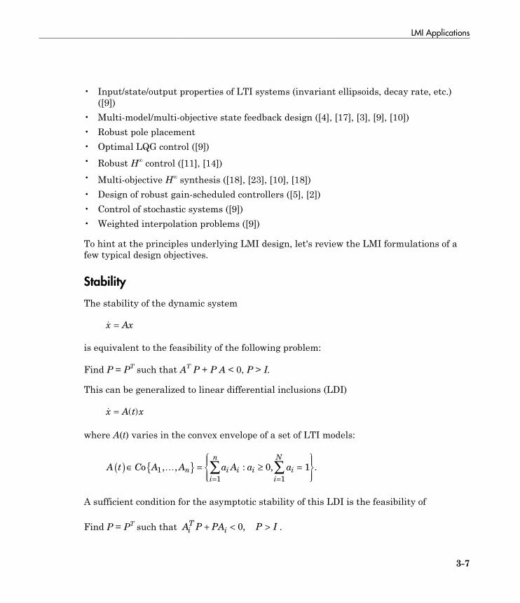
LMI Applications
3-7
• Input/state/output properties of LTI systems (invariant ellipsoids, decay rate, etc.)([9])
• Multi-model/multi-objective state feedback design ([4], [17], [3], [9], [10])• Robust pole placement• Optimal LQG control ([9])• Robust H∞ control ([11], [14])• Multi-objective H∞ synthesis ([18], [23], [10], [18])• Design of robust gain-scheduled controllers ([5], [2])• Control of stochastic systems ([9])• Weighted interpolation problems ([9])
To hint at the principles underlying LMI design, let's review the LMI formulations of afew typical design objectives.
Stability
The stability of the dynamic system
&x Ax=
is equivalent to the feasibility of the following problem:
Find P = PT such that AT P + P A < 0, P > I.
This can be generalized to linear differential inclusions (LDI)
&x A t x= ( )
where A(t) varies in the convex envelope of a set of LTI models:
A t C A A a A a an i i i i
i
N
i
n
( )Œ { } = ≥ =ÏÌÔ
ÓÔ
¸˝Ô
Ô==ÂÂo 1, , : , .… 0 1
11
A sufficient condition for the asymptotic stability of this LDI is the feasibility of
Find P = PT such that A P PA P IiT
i+ < >0, .

3 Introduction to Linear Matrix Inequalities
3-8
RMS Gain
The random-mean-squares (RMS) gain of a stable LTI system
&x Ax Bu
y Cx Du
= +
= +
ÏÌÓ
is the largest input/output gain over all bounded inputs u(t). This gain is the globalminimum of the following linear objective minimization problem [1], [25], [26].
Minimize γ over X = XT and γ such that
A X XA XB C
B X I D
C D I
T T
T T
+
--
Ê
Ë
ÁÁÁÁ
ˆ
¯
˜˜˜˜
<gg
0
and
X > 0.
LQG Performance
For a stable LTI system
Gx Ax Bw
y Cx
& = +
=
ÏÌÓ
where w is a white noise disturbance with unit covariance, the LQG or H2 performance∥G∥2 is defined by
G ET
y t y t dt
G j G j d
T
TT
H
2
2
0
1
1
2
: lim
.
= ( ) ( )ÏÌÔ
ÓÔ
¸˝Ô
Ô
= ( ) ( )
Æ•
-•
Ú
pw w w
••
Ú
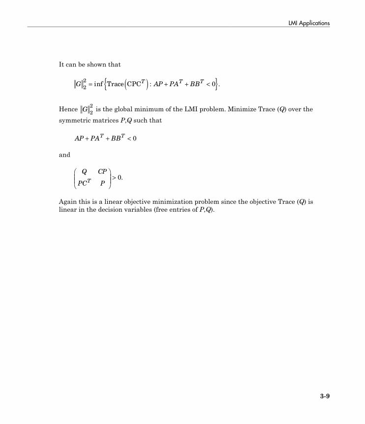
LMI Applications
3-9
It can be shown that
G AP PA BBT T T
2
20= ( ) + + <{ }inf : .Trace CPC
Hence G2
2 is the global minimum of the LMI problem. Minimize Trace (Q) over thesymmetric matrices P,Q such that
AP PA BBT T
+ + < 0
and
Q CP
PC PT
Ê
ËÁÁ
ˆ
¯˜ > 0.
Again this is a linear objective minimization problem since the objective Trace (Q) islinear in the decision variables (free entries of P,Q).
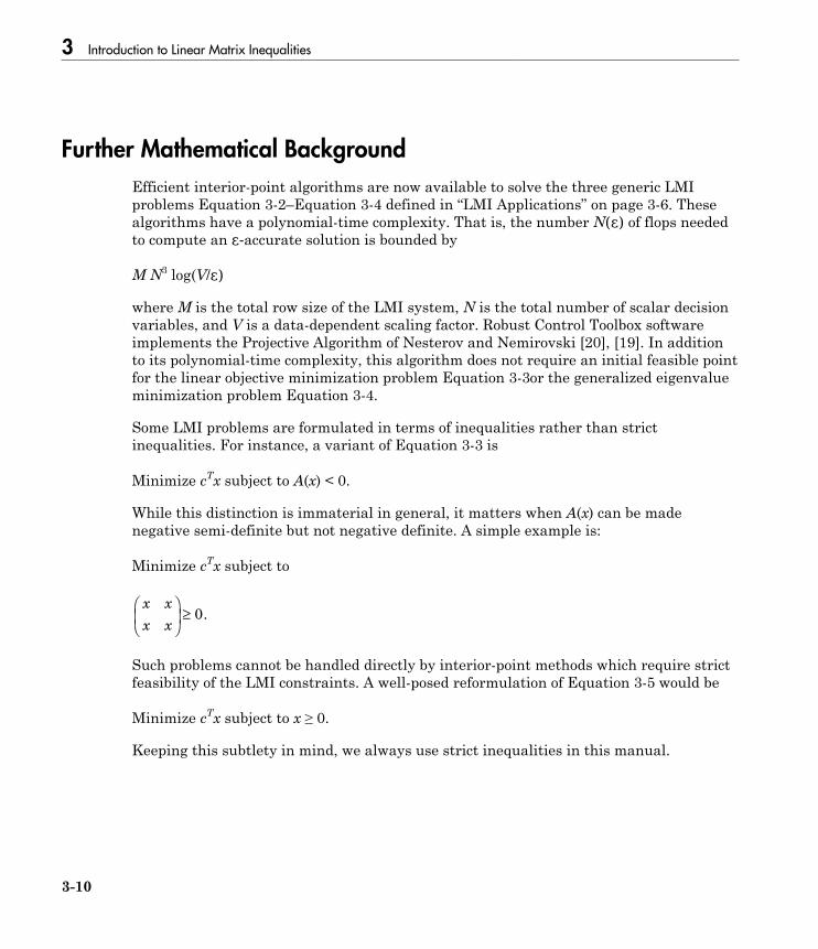
3 Introduction to Linear Matrix Inequalities
3-10
Further Mathematical Background
Efficient interior-point algorithms are now available to solve the three generic LMIproblems Equation 3-2–Equation 3-4 defined in “LMI Applications” on page 3-6. Thesealgorithms have a polynomial-time complexity. That is, the number N(ɛ) of flops neededto compute an ɛ-accurate solution is bounded by
M N3 log(V/ɛ)
where M is the total row size of the LMI system, N is the total number of scalar decisionvariables, and V is a data-dependent scaling factor. Robust Control Toolbox softwareimplements the Projective Algorithm of Nesterov and Nemirovski [20], [19]. In additionto its polynomial-time complexity, this algorithm does not require an initial feasible pointfor the linear objective minimization problem Equation 3-3or the generalized eigenvalueminimization problem Equation 3-4.
Some LMI problems are formulated in terms of inequalities rather than strictinequalities. For instance, a variant of Equation 3-3 is
Minimize cTx subject to A(x) < 0.
While this distinction is immaterial in general, it matters when A(x) can be madenegative semi-definite but not negative definite. A simple example is:
Minimize cTx subject to
x x
x x
Ê
ËÁ
ˆ
¯˜ ≥ 0.
Such problems cannot be handled directly by interior-point methods which require strictfeasibility of the LMI constraints. A well-posed reformulation of Equation 3-5 would be
Minimize cTx subject to x ≥ 0.
Keeping this subtlety in mind, we always use strict inequalities in this manual.
Bibliography
3-11
Bibliography
[1] Anderson, B.D.O., and S. Vongpanitlerd, Network Analysis, Prentice-Hall, EnglewoodCliffs, 1973.
[2] Apkarian, P., P. Gahinet, and G. Becker, “Self-Scheduled H∞ Control of LinearParameter-Varying Systems,” Proc. Amer. Contr. Conf., 1994, pp. 856-860.
[3] Bambang, R., E. Shimemura, and K. Uchida, “Mixed H2 /H∞ Control with PolePlacement,” State-Feedback Case, Proc. Amer. Contr. Conf., 1993, pp. 2777-2779.
[4] Barmish, B.R., “Stabilization of Uncertain Systems via Linear Control,” IEEE Trans.Aut. Contr., AC–28 (1983), pp. 848-850.
[5] Becker, G., and Packard, P., “Robust Performance of Linear-Parametrically VaryingSystems Using Parametrically-Dependent Linear Feedback,” Systems andControl Letters, 23 (1994), pp. 205-215.
[6] Bendsoe, M.P., A. Ben-Tal, and J. Zowe, “Optimization Methods for Truss Geometryand Topology Design,” to appear in Structural Optimization.
[7] Ben-Tal, A., and A. Nemirovski, “Potential Reduction Polynomial-Time Method forTruss Topology Design,” to appear in SIAM J. Contr. Opt.
[8] Boyd, S., and Q. Yang, “Structured and Simultaneous Lyapunov Functions for SystemStability Problems,” Int. J. Contr., 49 (1989), pp. 2215-2240.
[9] Boyd, S., L. El Ghaoui, E. Feron, and V. Balakrishnan, Linear Matrix Inequalities inSystems and Control Theory, SIAM books, Philadelphia, 1994.
[10] Chilali, M., and P. Gahinet, “H∞ Design with Pole Placement Constraints: an LMIApproach,” to appear in IEEE Trans. Aut. Contr. Also in Proc. Conf. Dec. Contr.,1994, pp. 553-558.
[11] Gahinet, P., and P. Apkarian, “A Linear Matrix Inequality Approach to H∞ Control,”Int. J. Robust and Nonlinear Contr., 4 (1994), pp. 421-448.
[12] Gahinet, P., P. Apkarian, and M. Chilali, “Affine Parameter-Dependent LyapunovFunctions for Real Parametric Uncertainty,“ Proc. Conf. Dec. Contr., 1994, pp.2026-2031.
3 Introduction to Linear Matrix Inequalities
3-12
[13] Haddad, W.M., and D.S. Berstein, “Parameter-Dependent Lyapunov Functions,Constant Real Parameter Uncertainty, and the Popov Criterion in RobustAnalysis and Synthesis: Part 1 and 2,” Proc. Conf. Dec. Contr., 1991, pp.2274-2279 and 2632-2633.
[14] Iwasaki, T., and R.E. Skelton, “All Controllers for the General H∞ Control Problem:LMI Existence Conditions and State-Space Formulas,” Automatica, 30 (1994), pp.1307-1317.
[15] Horisberger, H.P., and P.R. Belanger, “Regulators for Linear Time-Varying Plantswith Uncertain Parameters,” IEEE Trans. Aut. Contr., AC–21 (1976), pp.705-708.
[16] How, J.P., and S.R. Hall, “Connection between the Popov Stability Criterion andBounds for Real Parameter Uncertainty,” Proc. Amer. Contr. Conf., 1993, pp.1084-1089.
[17] Khargonekar, P.P., and M.A. Rotea, “Mixed H2 /H∞ Control: a Convex OptimizationApproach,” IEEE Trans. Aut. Contr., 39 (1991), pp. 824-837.
[18] Masubuchi, I., A. Ohara, and N. Suda, “LMI-Based Controller Synthesis: A UnifiedFormulation and Solution,” submitted to Int. J. Robust and Nonlinear Contr.,1994.
[19] Nemirovski, A., and P. Gahinet, “The Projective Method for Solving Linear MatrixInequalities,” Proc. Amer. Contr. Conf., 1994, pp. 840-844.
[20] Nesterov, Yu, and A. Nemirovski, Interior Point Polynomial Methods in ConvexProgramming: Theory and Applications, SIAM Books, Philadelphia, 1994.
[21] Packard, A., and J.C. Doyle, “The Complex Structured Singular Value,” Automatica,29 (1994), pp. 71-109.
[22] Popov, V.M., “Absolute Stability of Nonlinear Systems of Automatic Control,”Automation and Remote Control, 22 (1962), pp. 857-875.
[23] Scherer, C., “Mixed H2 H∞ Control,” to appear in Trends in Control: A EuropeanPerspective, volume of the special contributions to the ECC 1995.
[24] Stein, G., and J.C. Doyle, “Beyond Singular Values and Loop Shapes,” J. Guidance,14 (1991), pp. 5-16.
Bibliography
3-13
[25] Vidyasagar, M., Nonlinear System Analysis, Prentice-Hall, Englewood Cliffs, 1992.
[26] Willems, J.C., “Least-Squares Stationary Optimal Control and the Algebraic RiccatiEquation,” IEEE Trans. Aut. Contr., AC–16 (1971), pp. 621-634.
[27] Young, P.M., M.P. Newlin, and J.C. Doyle, “Let's Get Real,” in Robust ControlTheory, Springer Verlag, 1994, pp. 143-174.
[28] Zames, G., “On the Input-Output Stability of Time-Varying Nonlinear FeedbackSystems, Part I and II,” IEEE Trans. Aut. Contr., AC–11 (1966), pp. 228-238 and465-476.

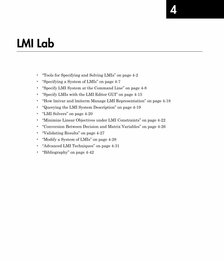
4
LMI Lab
• “Tools for Specifying and Solving LMIs” on page 4-2• “Specifying a System of LMIs” on page 4-7• “Specify LMI System at the Command Line” on page 4-8• “Specify LMIs with the LMI Editor GUI” on page 4-15• “How lmivar and lmiterm Manage LMI Representation” on page 4-18• “Querying the LMI System Description” on page 4-19• “LMI Solvers” on page 4-20• “Minimize Linear Objectives under LMI Constraints” on page 4-22• “Conversion Between Decision and Matrix Variables” on page 4-26• “Validating Results” on page 4-27• “Modify a System of LMIs” on page 4-28• “Advanced LMI Techniques” on page 4-31• “Bibliography” on page 4-42
4 LMI Lab
4-2
Tools for Specifying and Solving LMIs
The LMI Lab is a high-performance package for solving general LMI problems. It blendssimple tools for the specification and manipulation of LMIs with powerful LMI solvers forthree generic LMI problems. Thanks to a structure-oriented representation of LMIs, thevarious LMI constraints can be described in their natural block-matrix form. Similarly,the optimization variables are specified directly as matrix variables with some givenstructure. Once an LMI problem is specified, it can be solved numerically by callingthe appropriate LMI solver. The three solvers feasp, mincx, and gevp constitute thecomputational engine of the LMI portion of Robust Control Toolbox software. Their highperformance is achieved through C-MEX implementation and by taking advantage of theparticular structure of each LMI.
The LMI Lab offers tools to
• Specify LMI systems either symbolically with the LMI Editor or incrementally withthe lmivar and lmiterm commands
• Retrieve information about existing systems of LMIs• Modify existing systems of LMIs• Solve the three generic LMI problems (feasibility problem, linear objective
minimization, and generalized eigenvalue minimization)• Validate results
This chapter gives a tutorial introduction to the LMI Lab as well as more advanced tipsfor making the most out of its potential.
Some Terminology
Any linear matrix inequality can be expressed in the canonical formL(x) = L0 + x1L1 + . . . + xNLN < 0
where
• L0, L1, . . . , LN are given symmetric matrices• x = (x1, . . . , xN)T ∊ RN is the vector of scalar variables to be determined. We refer to
x1, . . . , xN as the decision variables. The names “design variables” and “optimizationvariables” are also found in the literature.

Tools for Specifying and Solving LMIs
4-3
Even though this canonical expression is generic, LMIs rarely arise in this form incontrol applications. Consider for instance the Lyapunov inequality
A X XAT
+ < 0
where
A =-
-Ê
ËÁ
ˆ
¯˜
1 2
0 2
and the variable
Xx x
x x=
Ê
ËÁ
ˆ
¯˜
1 2
2 3
is a symmetric matrix. Here the decision variables are the free entries x1, x2, x3 of X andthe canonical form of this LMI reads
x x x1 2 3
2 2
2 0
0 3
3 4
0 0
0 40
-Ê
ËÁ
ˆ
¯˜ +
--
Ê
ËÁ
ˆ
¯˜ +
-Ê
ËÁ
ˆ
¯˜ < .
Clearly this expression is less intuitive and transparent than Equation 4-1. Moreover,the number of matrices involved in Equation 4-2 grows roughly as n2 /2 if n is the size ofthe A matrix. Hence, the canonical form is very inefficient from a storage viewpoint sinceit requires storing o(n2 /2) matrices of size n when the single n-by-n matrix A would besufficient. Finally, working with the canonical form is also detrimental to the efficiency ofthe LMI solvers. For these various reasons, the LMI Lab uses a structured representationof LMIs. For instance, the expression ATX + XA in the Lyapunov inequality Equation 4-1is explicitly described as a function of the matrix variable X, and only the A matrix isstored.
In general, LMIs assume a block matrix form where each block is an affine combinationof the matrix variables. As a fairly typical illustration, consider the following LMI drawnfrom H∞ theory
N
A X XA XC B
CX I D
B D I
NT
T T
T T
+-
-
Ê
Ë
ÁÁÁÁ
ˆ
¯
˜˜˜
<g
g
0
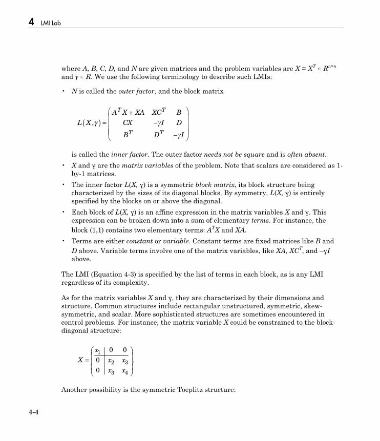
4 LMI Lab
4-4
where A, B, C, D, and N are given matrices and the problem variables are X = XT ∊ Rn×n
and γ ∊ R. We use the following terminology to describe such LMIs:
• N is called the outer factor, and the block matrix
L X
A X XA XC B
CX I D
B D I
T T
T T
,g g
g
( ) =+
-
-
Ê
Ë
ÁÁÁÁ
ˆ
¯
˜˜˜
is called the inner factor. The outer factor needs not be square and is often absent.• X and γ are the matrix variables of the problem. Note that scalars are considered as 1-
by-1 matrices.• The inner factor L(X, γ) is a symmetric block matrix, its block structure being
characterized by the sizes of its diagonal blocks. By symmetry, L(X, γ) is entirelyspecified by the blocks on or above the diagonal.
• Each block of L(X, γ) is an affine expression in the matrix variables X and γ. Thisexpression can be broken down into a sum of elementary terms. For instance, theblock (1,1) contains two elementary terms: ATX and XA.
• Terms are either constant or variable. Constant terms are fixed matrices like B andD above. Variable terms involve one of the matrix variables, like XA, XCT, and –γIabove.
The LMI (Equation 4-3) is specified by the list of terms in each block, as is any LMIregardless of its complexity.
As for the matrix variables X and γ, they are characterized by their dimensions andstructure. Common structures include rectangular unstructured, symmetric, skew-symmetric, and scalar. More sophisticated structures are sometimes encountered incontrol problems. For instance, the matrix variable X could be constrained to the block-diagonal structure:
X
x
x x
x x
=Ê
Ë
ÁÁÁ
ˆ
¯
˜˜˜
1
2 3
3 4
0 0
0
0
.
Another possibility is the symmetric Toeplitz structure:
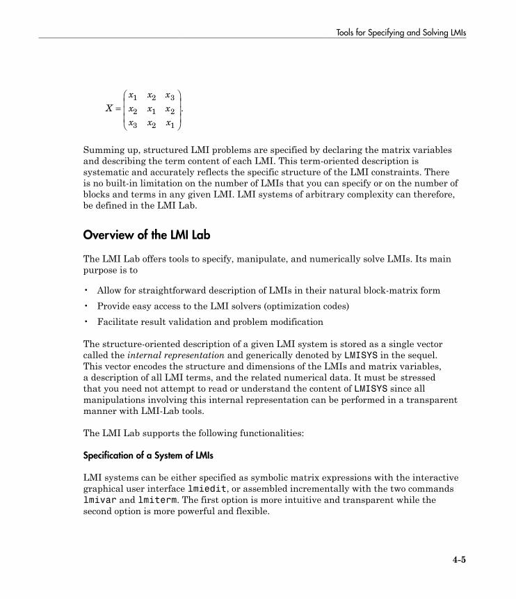
Tools for Specifying and Solving LMIs
4-5
X
x x x
x x x
x x x
=Ê
Ë
ÁÁÁ
ˆ
¯
˜˜˜
1 2 3
2 1 2
3 2 1
.
Summing up, structured LMI problems are specified by declaring the matrix variablesand describing the term content of each LMI. This term-oriented description issystematic and accurately reflects the specific structure of the LMI constraints. Thereis no built-in limitation on the number of LMIs that you can specify or on the number ofblocks and terms in any given LMI. LMI systems of arbitrary complexity can therefore,be defined in the LMI Lab.
Overview of the LMI Lab
The LMI Lab offers tools to specify, manipulate, and numerically solve LMIs. Its mainpurpose is to
• Allow for straightforward description of LMIs in their natural block-matrix form• Provide easy access to the LMI solvers (optimization codes)• Facilitate result validation and problem modification
The structure-oriented description of a given LMI system is stored as a single vectorcalled the internal representation and generically denoted by LMISYS in the sequel.This vector encodes the structure and dimensions of the LMIs and matrix variables,a description of all LMI terms, and the related numerical data. It must be stressedthat you need not attempt to read or understand the content of LMISYS since allmanipulations involving this internal representation can be performed in a transparentmanner with LMI-Lab tools.
The LMI Lab supports the following functionalities:
Specification of a System of LMIs
LMI systems can be either specified as symbolic matrix expressions with the interactivegraphical user interface lmiedit, or assembled incrementally with the two commandslmivar and lmiterm. The first option is more intuitive and transparent while thesecond option is more powerful and flexible.

4 LMI Lab
4-6
Information Retrieval
The interactive function lmiinfo answers qualitative queries about LMI systemscreated with lmiedit or lmivar and lmiterm. You can also use lmiedit to visualizethe LMI system produced by a particular sequence of lmivar/lmiterm commands.
Solvers for LMI Optimization Problems
General-purpose LMI solvers are provided for the three generic LMI problems defined in“LMI Applications” on page 3-6. These solvers can handle very general LMI systems andmatrix variable structures. They return a feasible or optimal vector of decision variablesx*. The corresponding values X X
K1* *, ,… of the matrix variables are given by the function
dec2mat.
Result Validation
The solution x* produced by the LMI solvers is easily validated with the functionsevallmi and showlmi. This allows a fast check and/or analysis of the results. Withevallmi, all variable terms in the LMI system are evaluated for the value x* of thedecision variables. The left and right sides of each LMI then become constant matricesthat can be displayed with showlmi.
Modification of a System of LMIs
An existing system of LMIs can be modified in two ways:
• An LMI can be removed from the system with dellmi.• A matrix variable X can be deleted using delmvar. It can also be instantiated, that is,
set to some given matrix value. This operation is performed by setmvar and allows,for example, to fix some variables and solve the LMI problem with respect to theremaining ones.
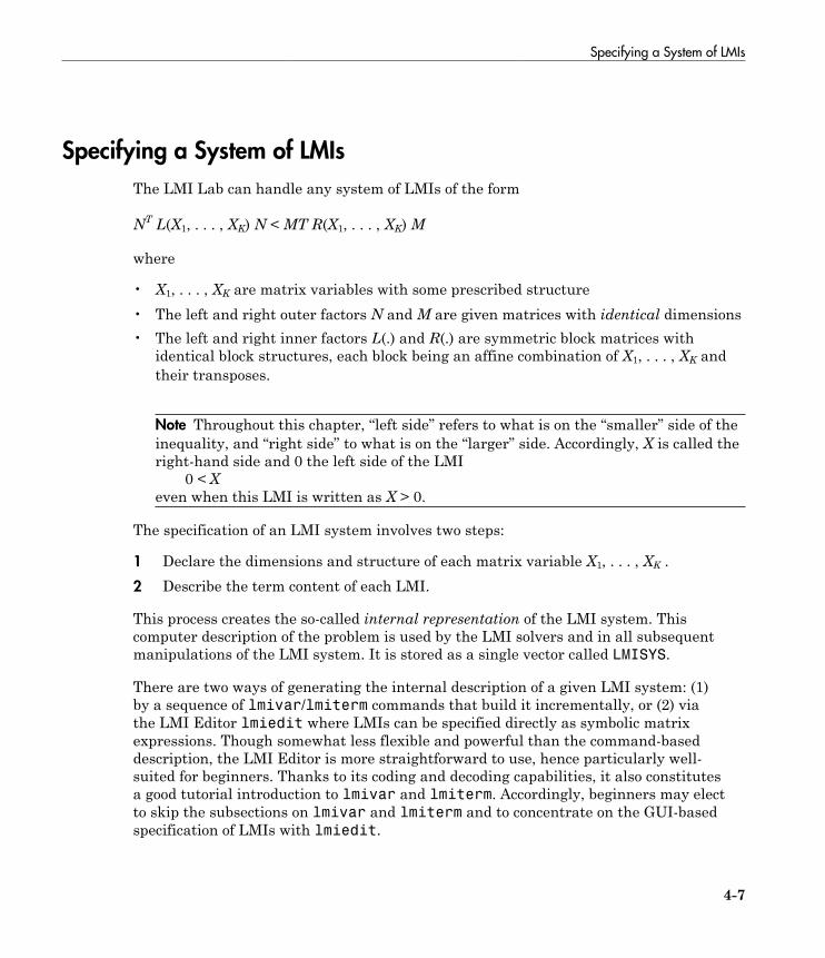
Specifying a System of LMIs
4-7
Specifying a System of LMIs
The LMI Lab can handle any system of LMIs of the form
NT L(X1, . . . , XK) N < MT R(X1, . . . , XK) M
where
• X1, . . . , XK are matrix variables with some prescribed structure• The left and right outer factors N and M are given matrices with identical dimensions• The left and right inner factors L(.) and R(.) are symmetric block matrices with
identical block structures, each block being an affine combination of X1, . . . , XK andtheir transposes.
Note Throughout this chapter, “left side” refers to what is on the “smaller” side of theinequality, and “right side” to what is on the “larger” side. Accordingly, X is called theright-hand side and 0 the left side of the LMI 0 < Xeven when this LMI is written as X > 0.
The specification of an LMI system involves two steps:
1 Declare the dimensions and structure of each matrix variable X1, . . . , XK .2 Describe the term content of each LMI.
This process creates the so-called internal representation of the LMI system. Thiscomputer description of the problem is used by the LMI solvers and in all subsequentmanipulations of the LMI system. It is stored as a single vector called LMISYS.
There are two ways of generating the internal description of a given LMI system: (1)by a sequence of lmivar/lmiterm commands that build it incrementally, or (2) viathe LMI Editor lmiedit where LMIs can be specified directly as symbolic matrixexpressions. Though somewhat less flexible and powerful than the command-baseddescription, the LMI Editor is more straightforward to use, hence particularly well-suited for beginners. Thanks to its coding and decoding capabilities, it also constitutesa good tutorial introduction to lmivar and lmiterm. Accordingly, beginners may electto skip the subsections on lmivar and lmiterm and to concentrate on the GUI-basedspecification of LMIs with lmiedit.
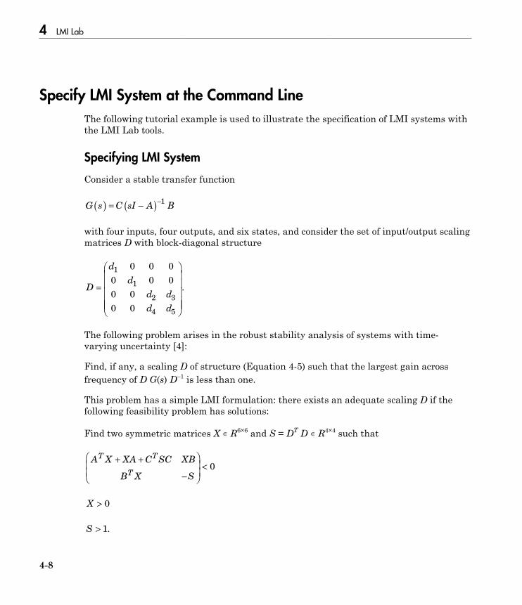
4 LMI Lab
4-8
Specify LMI System at the Command Line
The following tutorial example is used to illustrate the specification of LMI systems withthe LMI Lab tools.
Specifying LMI System
Consider a stable transfer function
G s C sI A B( ) = -( )-1
with four inputs, four outputs, and six states, and consider the set of input/output scalingmatrices D with block-diagonal structure
D
d
d
d d
d d
=
Ê
Ë
ÁÁÁÁÁ
ˆ
¯
˜˜˜˜
1
1
2 3
4 5
0 0 0
0 0 0
0 0
0 0
.
The following problem arises in the robust stability analysis of systems with time-varying uncertainty [4]:
Find, if any, a scaling D of structure (Equation 4-5) such that the largest gain acrossfrequency of D G(s) D–1 is less than one.
This problem has a simple LMI formulation: there exists an adequate scaling D if thefollowing feasibility problem has solutions:
Find two symmetric matrices X ∊ R6×6 and S = DT D ∊ R4×4 such that
A X XA C SC XB
B X S
T T
T
+ +
-
Ê
ËÁÁ
ˆ
¯˜˜
< 0
X > 0
S > 1.
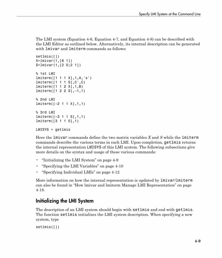
Specify LMI System at the Command Line
4-9
The LMI system (Equation 4-6, Equation 4-7, and Equation 4-8) can be described withthe LMI Editor as outlined below. Alternatively, its internal description can be generatedwith lmivar and lmiterm commands as follows:
setlmis([])
X=lmivar(1,[6 1])
S=lmivar(1,[2 0;2 1])
% 1st LMI
lmiterm([1 1 1 X],1,A,'s')
lmiterm([1 1 1 S],C',C)
lmiterm([1 1 2 X],1,B)
lmiterm([1 2 2 S],–1,1)
% 2nd LMI
lmiterm([–2 1 1 X],1,1)
% 3rd LMI
lmiterm([–3 1 1 S],1,1)
lmiterm([3 1 1 0],1)
LMISYS = getlmis
Here the lmivar commands define the two matrix variables X and S while the lmitermcommands describe the various terms in each LMI. Upon completion, getlmis returnsthe internal representation LMISYS of this LMI system. The following subsections givemore details on the syntax and usage of these various commands:
• “Initializing the LMI System” on page 4-9• “Specifying the LMI Variables” on page 4-10• “Specifying Individual LMIs” on page 4-12
More information on how the internal representation is updated by lmivar/lmitermcan also be found in “How lmivar and lmiterm Manage LMI Representation” on page4-18.
Initializing the LMI System
The description of an LMI system should begin with setlmis and end with getlmis.The function setlmis initializes the LMI system description. When specifying a newsystem, type
setlmis([])
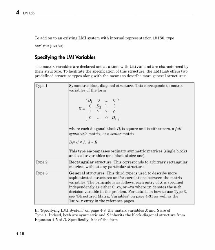
4 LMI Lab
4-10
To add on to an existing LMI system with internal representation LMIS0, type
setlmis(LMIS0)
Specifying the LMI Variables
The matrix variables are declared one at a time with lmivar and are characterized bytheir structure. To facilitate the specification of this structure, the LMI Lab offers twopredefined structure types along with the means to describe more general structures:
Type 1 Symmetric block diagonal structure. This corresponds to matrixvariables of the form
X
D
D
Dr
=
Ê
Ë
ÁÁÁÁÁ
ˆ
¯
˜˜˜˜
1
2
0 0
0
0
0 0
…
O M
M O O
…
where each diagonal block Dj is square and is either zero, a fullsymmetric matrix, or a scalar matrix
Dj= d × I, d ∊ R
This type encompasses ordinary symmetric matrices (single block)and scalar variables (one block of size one).
Type 2 Rectangular structure. This corresponds to arbitrary rectangularmatrices without any particular structure.
Type 3 General structures. This third type is used to describe moresophisticated structures and/or correlations between the matrixvariables. The principle is as follows: each entry of X is specifiedindependently as either 0, xn, or –xn where xn denotes the n-thdecision variable in the problem. For details on how to use Type 3,see “Structured Matrix Variables” on page 4-31 as well as thelmivar entry in the reference pages.
In “Specifying LMI System” on page 4-8, the matrix variables X and S are ofType 1. Indeed, both are symmetric and S inherits the block-diagonal structure fromEquation 4-5 of D. Specifically, S is of the form
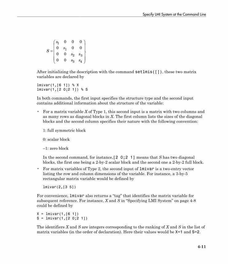
Specify LMI System at the Command Line
4-11
S
s
s
s s
s s
=
Ê
Ë
ÁÁÁÁÁ
ˆ
¯
˜˜˜˜
1
1
2 3
3 4
0 0 0
0 0 0
0 0
0 0
.
After initializing the description with the command setlmis([]), these two matrixvariables are declared by
lmivar(1,[6 1]) % X
lmivar(1,[2 0;2 1]) % S
In both commands, the first input specifies the structure type and the second inputcontains additional information about the structure of the variable:
• For a matrix variable X of Type 1, this second input is a matrix with two columns andas many rows as diagonal blocks in X. The first column lists the sizes of the diagonalblocks and the second column specifies their nature with the following convention:
1: full symmetric block
0: scalar block
–1: zero block
In the second command, for instance,[2 0;2 1] means that S has two diagonalblocks, the first one being a 2-by-2 scalar block and the second one a 2-by-2 full block.
• For matrix variables of Type 2, the second input of lmivar is a two-entry vectorlisting the row and column dimensions of the variable. For instance, a 3-by-5rectangular matrix variable would be defined by
lmivar(2,[3 5])
For convenience, lmivar also returns a “tag” that identifies the matrix variable forsubsequent reference. For instance, X and S in “Specifying LMI System” on page 4-8could be defined by
X = lmivar(1,[6 1])
S = lmivar(1,[2 0;2 1])
The identifiers X and S are integers corresponding to the ranking of X and S in the list ofmatrix variables (in the order of declaration). Here their values would be X=1 and S=2.
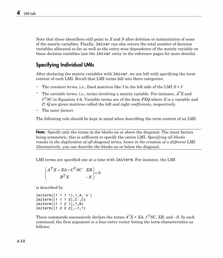
4 LMI Lab
4-12
Note that these identifiers still point to X and S after deletion or instantiation of someof the matrix variables. Finally, lmivar can also return the total number of decisionvariables allocated so far as well as the entry-wise dependence of the matrix variable onthese decision variables (see the lmivar entry in the reference pages for more details).
Specifying Individual LMIs
After declaring the matrix variables with lmivar, we are left with specifying the termcontent of each LMI. Recall that LMI terms fall into three categories:
• The constant terms, i.e., fixed matrices like I in the left side of the LMI S > I• The variable terms, i.e., terms involving a matrix variable. For instance, ATX and
CTSC in Equation 4-6. Variable terms are of the form PXQ where X is a variable andP, Q are given matrices called the left and right coefficients, respectively.
• The outer factors
The following rule should be kept in mind when describing the term content of an LMI:
Note: Specify only the terms in the blocks on or above the diagonal. The inner factorsbeing symmetric, this is sufficient to specify the entire LMI. Specifying all blocksresults in the duplication of off-diagonal terms, hence in the creation of a different LMI.Alternatively, you can describe the blocks on or below the diagonal.
LMI terms are specified one at a time with lmiterm. For instance, the LMI
A X XA C SC XB
B X S
T T
T
+ +
-
Ê
ËÁÁ
ˆ
¯˜˜
< 0
is described by
lmiterm([1 1 1 1],1,A,'s')
lmiterm([1 1 1 2],C',C)
lmiterm([1 1 2 1],1,B)
lmiterm([1 2 2 2],–1,1)
These commands successively declare the terms ATX + XA, CTSC, XB, and –S. In eachcommand, the first argument is a four-entry vector listing the term characteristics asfollows:

Specify LMI System at the Command Line
4-13
• The first entry indicates to which LMI the term belongs. The value m means “left sideof the m-th LMI,” and −m means “right side of the m-th LMI.”
• The second and third entries identify the block to which the term belongs. Forinstance, the vector [1 1 2 1] indicates that the term is attached to the (1, 2) block.
• The last entry indicates which matrix variable is involved in the term. This entry is 0for constant terms, k for terms involving the k-th matrix variable Xk, and −k for terms
involving XkT (here X and S are first and second variables in the order of declaration).
Finally, the second and third arguments of lmiterm contain the numerical data (valuesof the constant term, outer factor, or matrix coefficients P and Q for variable terms PXQor PXTQ). These arguments must refer to existing MATLAB variables and be real-valued.See “Complex-Valued LMIs” on page 4-33 for the specification of LMIs with complex-valued coefficients.
Some shorthand is provided to simplify term specification. First, blocks are zero bydefault. Second, in diagonal blocks the extra argument 's' allows you to specify theconjugated expression AXB + BTXTAT with a single lmiterm command. For instance,the first command specifies ATX + XA as the “symmetrization” of XA. Finally, scalarvalues are allowed as shorthand for scalar matrices, i.e., matrices of the form αI with αscalar. Thus, a constant term of the form αI can be specified as the “scalar” α. This alsoapplies to the coefficients P and Q of variable terms. The dimensions of scalar matricesare inferred from the context and set to 1 by default. For instance, the third LMI S > I in“Example: Specifying Matrix Variable Structures” on page 4-31 is described by
lmiterm([–3 1 1 2],1,1) % 1*S*1 = S
lmiterm([3 1 1 0],1) % 1*I = I
Recall that by convention S is considered as the right side of the inequality, whichjustifies the –3 in the first command.
Finally, to improve readability it is often convenient to attach an identifier (tag) to eachLMI and matrix variable. The variable identifiers are returned by lmivar and the LMIidentifiers are set by the function newlmi. These identifiers can be used in lmitermcommands to refer to a given LMI or matrix variable. For the LMI system of “SpecifyingLMI System” on page 4-8, this would look like:
setlmis([])
X = lmivar(1,[6 1])
S = lmivar(1,[2 0;2 1])

4 LMI Lab
4-14
BRL = newlmi
lmiterm([BRL 1 1 X],1,A,'s')
lmiterm([BRL 1 1 S],C',C)
lmiterm([BRL 1 2 X],1,B)
lmiterm([BRL 2 2 S],–1,1)
Xpos = newlmi
lmiterm([-Xpos 1 1 X],1,1)
Slmi = newlmi
lmiterm([-Slmi 1 1 S],1,1)
lmiterm([Slmi 1 1 0],1)
When the LMI system is completely specified, type
LMISYS = getlmis
This returns the internal representation LMISYS of this LMI system. This MATLABdescription of the problem can be forwarded to other LMI-Lab functions for subsequentprocessing. The command getlmis must be used only once and after declaring all matrixvariables and LMI terms.
Here the identifiers X and S point to the variables X and S while the tags BRL, Xpos, andSlmi point to the first, second, and third LMI, respectively. Note that –Xpos refers tothe right-hand side of the second LMI. Similarly, –X would indicate transposition of thevariable X.
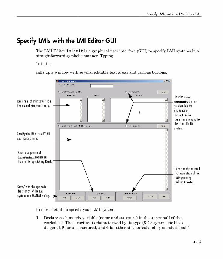
Specify LMIs with the LMI Editor GUI
4-15
Specify LMIs with the LMI Editor GUI
The LMI Editor lmiedit is a graphical user interface (GUI) to specify LMI systems in astraightforward symbolic manner. Typing
lmiedit
calls up a window with several editable text areas and various buttons.
In more detail, to specify your LMI system,
1 Declare each matrix variable (name and structure) in the upper half of theworksheet. The structure is characterized by its type (S for symmetric blockdiagonal, R for unstructured, and G for other structures) and by an additional “
4 LMI Lab
4-16
structure” matrix. This matrix contains specific information about the structure andcorresponds to the second argument of lmivar (see “Specifying the LMI Variables”on page 4-10 for details).
Please use one line per matrix variable in the text editing areas.2 Specify the LMIs as MATLAB expressions in the lower half of the worksheet. For
instance, the LMI
A X XA XB
B X I
T
T
+
-
Ê
ËÁÁ
ˆ
¯˜˜
< 0
is entered by typing
[a'*x+x*a x*b; b'*x –1] < 0
if x is the name given to the matrix variable X in the upper half of the worksheet.The left- and right-hand sides of the LMIs should be valid MATLAB expressions.
Once the LMI system is fully specified, the following tasks can be performed by clickingthe corresponding button:
• Visualize the sequence of lmivar/lmiterm commands needed to describe this LMIsystem (view commands button). Conversely, the LMI system defined by a particularsequence of lmivar/lmiterm commands can be displayed as a MATLAB expressionby clicking on the describe... buttons.
Beginners can use this facility as a tutorial introduction to the lmivar and lmitermcommands.
• Save the symbolic description of the LMI system as a MATLAB string (save button).This description can be reloaded later on by clicking the load button.
• Read a sequence of lmivar/lmiterm commands from a file (read button). You canthen click on describe the matrix variables or describe the LMIs to visualize thesymbolic expression of the LMI system specified by these commands. The file shoulddescribe a single LMI system but may otherwise contain any sequence of MATLABcommands.
This feature is useful for code validation and debugging.
Write in a file the sequence of lmivar/lmiterm commands needed to describe aparticular LMI system (write button).
Specify LMIs with the LMI Editor GUI
4-17
This is helpful to develop code and prototype MATLAB functions based on the LMILab.
• Generate the internal representation of the LMI system by clicking create. The resultis written in a MATLAB variable named after the LMI system (if the “name of theLMI system” is set to mylmi, the internal representation is written in the MATLABvariable mylmi). Note that all LMI-related data should be defined in the MATLABworkspace at this stage.
The internal representation can be passed directly to the LMI solvers or any otherLMI Lab function.
Keyboard Shortcuts
As with lmiterm, you can use various shortcuts when entering LMI expressions atthe keyboard. For instance, zero blocks can be entered simply as 0 and need not bedimensioned. Similarly, the identity matrix can be entered as 1 without dimensioning.Finally, upper diagonal LMI blocks need not be fully specified. Rather, you can just type(*) in place of each such block.
Limitations
Though fairly general, lmiedit is not as flexible as lmiterm and the followinglimitations should be kept in mind:
• Parentheses cannot be used around matrix variables. For instance, the expression
(a*x+b)'*c + c'*(a*x+b)
is invalid when x is a variable name. By contrast,
(a+b)'*x + x'*(a+b)
is perfectly valid.• Loops and if statements are ignored.• When turning lmiterm commands into a symbolic description of the LMI system, an
error is issued if the first argument of lmiterm cannot be evaluated. Use the LMI andvariable identifiers supplied by newlmi and lmivar to avoid such difficulties.
4 LMI Lab
4-18
How lmivar and lmiterm Manage LMI Representation
Users familiar with MATLAB may wonder how lmivar and lmiterm physically updatethe internal representation LMISYS since LMISYS is not an argument to these functions.In fact, all updating is performed through global variables for maximum speed. Theseglobal variables are initialized by setlmis, cleared by getlmis, and are not visible inthe workspace. Even though this artifact is transparent from the user's viewpoint, besure to
• Invoke getlmis only once and after completely specifying the LMI system• Refrain from using the command clear global before the LMI system description is
ended with getlmis
Querying the LMI System Description
4-19
Querying the LMI System Description
Recall that the full description of an LMI system is stored as a single vector called theinternal representation. The user should not attempt to read or retrieve informationdirectly from this vector. Robust Control Toolbox software provides three functions calledlmiinfo, lminbr, and matnbr to extract and display all relevant information in a user-readable format.
lmiinfo
lminbr is an interactive facility to retrieve qualitative information about LMI systems.This includes the number of LMIs, the number of matrix variables and their structure,the term content of each LMI block, etc. To invoke lmiinfo, enter
lmiinfo(LMISYS)
where LMISYS is the internal representation of the LMI system produced by getlmis.
lminbr and matnbr
These two functions return the number of LMIs and the number of matrix variables inthe system. To get the number of matrix variables, for instance, enter
matnbr(LMISYS)
4 LMI Lab
4-20
LMI Solvers
LMI solvers are provided for the following three generic optimization problems (here xdenotes the vector of decision variables, i.e., of the free entries of the matrix variablesX1, . . . , XK):
• Feasibility problem
Find x ∊ RN (or equivalently matrices X1, . . . , XK with prescribed structure) thatsatisfies the LMI system
A(x) < B(x)
The corresponding solver is called feasp.• Minimization of a linear objective under LMI constraints
Minimize cTx over x ∊ RN subject to A(x) < B(x)
The corresponding solver is called mincx.• Generalized eigenvalue minimization problem
Minimize λ over x ∊ RN subject to
C(x) < D(x)
0 < B(x)
A(x) < λB(x).
The corresponding solver is called gevp.
Note that A(x) < B(x) above is a shorthand notation for general structured LMI systemswith decision variables x = (x1, . . . , xN).
The three LMI solvers feasp, mincx, and gevp take as input the internal representationLMISYS of an LMI system and return a feasible or optimizing value x* of the decisionvariables. The corresponding values of the matrix variables X1, . . . , XK are derivedfrom x* with the function dec2mat. These solvers are C-MEX implementations of thepolynomial-time Projective Algorithm Projective Algorithm of Nesterov and Nemirovski[3], [2].
LMI Solvers
4-21
For generalized eigenvalue minimization problems, it is necessary to distinguish betweenthe standard LMI constraints C(x) < D(x) and the linear-fractional LMIs
A(x) < λB(x)
attached to the minimization of the generalized eigenvalue λ. When using gevp, youshould follow these three rules to ensure proper specification of the problem:
• Specify the LMIs involving λ as A(x) < B(x) (without the λ)• Specify them last in the LMI system. gevp systematically assumes that the last L
LMIs are linear-fractional if L is the number of LMIs involving λ• Add the constraint 0 < B(x) or any other constraint that enforces it. This positivity
constraint is required for well-posedness of the problem and is not automaticallyadded by gevp.
An initial guess xinit for x can be supplied to mincx or gevp. Use mat2dec to derivexinit from given values of the matrix variables X1, . . . , XK.
The following example illustrates the use of the mincx solver.
4 LMI Lab
4-22
Minimize Linear Objectives under LMI Constraints
Consider the optimization problem:
Minimize Trace(X) subject to
ATX + XA + XBBTX + Q < 0
with data
A B Q=- -
- -
Ê
Ë
ÁÁÁ
ˆ
¯
˜˜˜
=Ê
Ë
ÁÁÁ
ˆ
¯
˜˜˜
=-
- - --
1 2 1
3 2 1
1 2 1
1
0
1
1 1 0
1 3 12
0 1
; ;
22 36-
Ê
Ë
ÁÁÁ
ˆ
¯
˜˜˜.
It can be shown that the minimizer X* is simply the stabilizing solution of the algebraicRiccati equation
ATX + XA + XBBTX + Q = 0
This solution can be computed directly with the Riccati solver care and compared to theminimizer returned by mincx.
From an LMI optimization standpoint, the problem specified in Equation 4-9 isequivalent to the following linear objective minimization problem:
Minimize Trace(X) subject to
A X XA Q XB
B X I
T
T
+ +
-
Ê
ËÁÁ
ˆ
¯˜˜
< 0.
Since Trace(X) is a linear function of the entries of X, this problem falls within the scopeof the mincx solver and can be numerically solved as follows:
1 Define the LMI constraint of Equation 4-9 by the sequence of commands
setlmis([])
X = lmivar(1,[3 1]) % variable X, full symmetric
lmiterm([1 1 1 X],1,a,'s')
lmiterm([1 1 1 0],q)
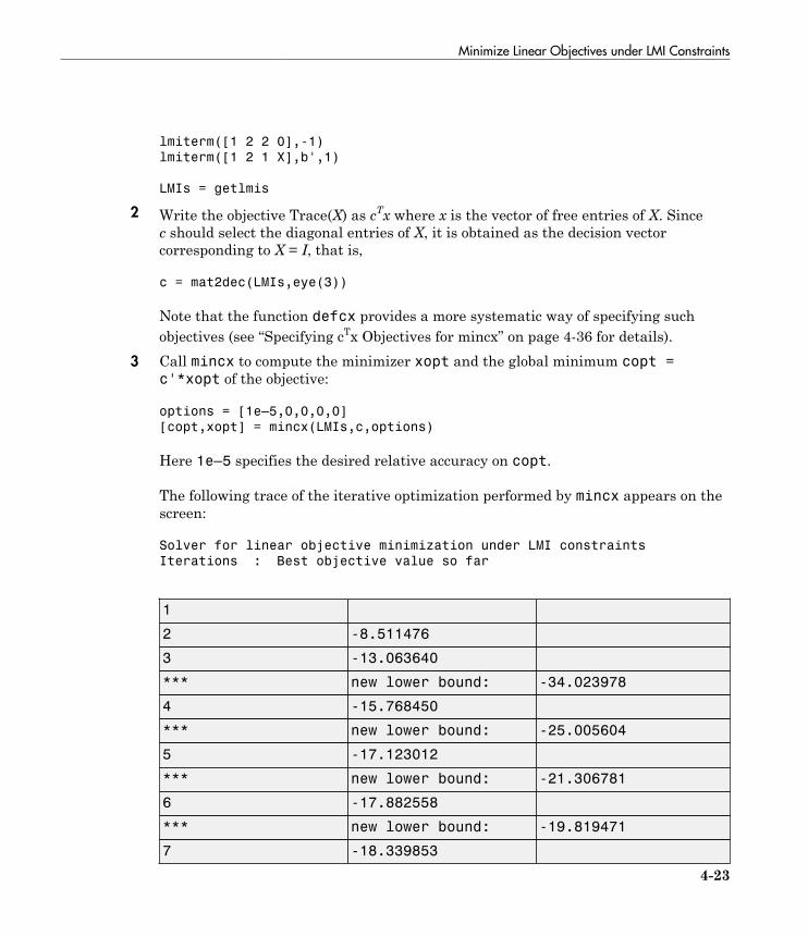
Minimize Linear Objectives under LMI Constraints
4-23
lmiterm([1 2 2 0],-1)
lmiterm([1 2 1 X],b',1)
LMIs = getlmis
2 Write the objective Trace(X) as cTx where x is the vector of free entries of X. Sincec should select the diagonal entries of X, it is obtained as the decision vectorcorresponding to X = I, that is,
c = mat2dec(LMIs,eye(3))
Note that the function defcx provides a more systematic way of specifying suchobjectives (see “Specifying cTx Objectives for mincx” on page 4-36 for details).
3 Call mincx to compute the minimizer xopt and the global minimum copt =c'*xopt of the objective:
options = [1e–5,0,0,0,0]
[copt,xopt] = mincx(LMIs,c,options)
Here 1e–5 specifies the desired relative accuracy on copt.
The following trace of the iterative optimization performed by mincx appears on thescreen:
Solver for linear objective minimization under LMI constraints
Iterations : Best objective value so far
1
2 -8.511476
3 -13.063640
*** new lower bound: -34.023978
4 -15.768450
*** new lower bound: -25.005604
5 -17.123012
*** new lower bound: -21.306781
6 -17.882558
*** new lower bound: -19.819471
7 -18.339853
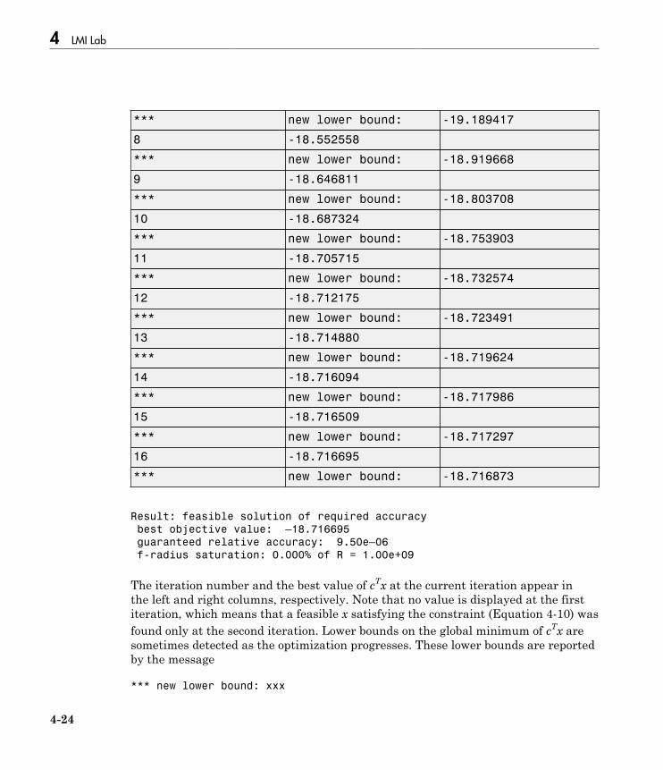
4 LMI Lab
4-24
*** new lower bound: -19.189417
8 -18.552558
*** new lower bound: -18.919668
9 -18.646811
*** new lower bound: -18.803708
10 -18.687324
*** new lower bound: -18.753903
11 -18.705715
*** new lower bound: -18.732574
12 -18.712175
*** new lower bound: -18.723491
13 -18.714880
*** new lower bound: -18.719624
14 -18.716094
*** new lower bound: -18.717986
15 -18.716509
*** new lower bound: -18.717297
16 -18.716695
*** new lower bound: -18.716873
Result: feasible solution of required accuracy
best objective value: –18.716695
guaranteed relative accuracy: 9.50e–06
f-radius saturation: 0.000% of R = 1.00e+09
The iteration number and the best value of cTx at the current iteration appear inthe left and right columns, respectively. Note that no value is displayed at the firstiteration, which means that a feasible x satisfying the constraint (Equation 4-10) wasfound only at the second iteration. Lower bounds on the global minimum of cTx aresometimes detected as the optimization progresses. These lower bounds are reportedby the message
*** new lower bound: xxx

Minimize Linear Objectives under LMI Constraints
4-25
Upon termination, mincx reports that the global minimum for the objective Trace(X)is –18.716695 with relative accuracy of at least 9.5×10⁻⁶. This is the value coptreturned by mincx.
4 mincx also returns the optimizing vector of decision variables xopt. Thecorresponding optimal value of the matrix variable X is given by
Xopt = dec2mat(LMIs,xopt,X)
which returns
Xopt =- -- -
-
6 3542 5 8895 2 2046
5 8895 6 2855 2 2201
2 2046 2 2201
. . .
. . .
. . 66 0771.
.
Ê
Ë
ÁÁÁ
ˆ
¯
˜˜˜
This result can be compared with the stabilizing Riccati solution computed by care:
Xst = care(a,b,q,–1)
norm(Xopt-Xst)
ans =
6.5390e–05
4 LMI Lab
4-26
Conversion Between Decision and Matrix Variables
While LMIs are specified in terms of their matrix variables X1, . . . , XK , the LMI solversoptimize the vector x of free scalar entries of these matrices, called the decision variables.The two functions mat2dec and dec2mat perform the conversion between these twodescriptions of the problem variables.
Consider an LMI system with three matrix variables X1, X2, X3. Given particular valuesX1, X2, X3 of these variables, the corresponding value xdec of the vector of decisionvariables is returned by mat2dec:
xdec = mat2dec(LMISYS,X1,X2,X3)
An error is issued if the number of arguments following LMISYS differs from the numberof matrix variables in the problem (see matnbr).
Conversely, given a value xdec of the vector of decision variables, the correspondingvalue of the k-th matrix is given by dec2mat. For instance, the value X2 of the secondmatrix variable is extracted from xdec by
X2 = dec2mat(LMISYS,xdec,2)
The last argument indicates that the second matrix variable is requested. It could be setto the matrix variable identifier returned by lmivar.
The total numbers of matrix variables and decision variables are returned by matnbrand decnbr, respectively. In addition, the function decinfo provides preciseinformation about the mapping between decision variables and matrix variable entries.

Validating Results
4-27
Validating Results
The LMI Lab offers two functions to analyze and validate the results of an LMIoptimization. The function evallmi evaluates all variable terms in an LMI system for agiven value of the vector of decision variables, for instance, the feasible or optimal vectorreturned by the LMI solvers. Once this evaluation is performed, the left and right sides ofa particular LMI are returned by showlmi.
In the LMI problem considered in “Minimize Linear Objectives under LMI Constraints”on page 4-22, you can verify that the minimizer xopt returned by mincx satisfies theLMI constraint (Equation 4-10) as follows:
evlmi = evallmi(LMIs,xopt)
[lhs,rhs] = showlmi(evlmi,1)
The first command evaluates the system for the value xopt of the decision variables,and the second command returns the left and right sides of the first (and only) LMI. Thenegative definiteness of this LMI is checked by
eig(lhs-rhs)
ans =
–2.0387e–04
–3.9333e–05
–1.8917e–07
–4.6680e+01
4 LMI Lab
4-28
Modify a System of LMIs
Once specified, a system of LMIs can be modified in several ways with the functionsdellmi, delmvar, and setmvar.
Deleting an LMI
The first possibility is to remove an entire LMI from the system with dellmi. Forinstance, suppose that the LMI system of “Specifying LMI System” on page 4-8 isdescribed in LMISYS and that we want to remove the positivity constraint on X. This isdone by
NEWSYS = dellmi(LMISYS,2)
where the second argument specifies deletion of the second LMI. The resulting system oftwo LMIs is returned in NEWSYS.
The LMI identifiers (initial ranking of the LMI in the LMI system) are not altered bydeletions. As a result, the last LMI
S > I
remains known as the third LMI even though it now ranks second in the modifiedsystem. To avoid confusion, it is safer to refer to LMIs via the identifiers returnedby newlmi. If BRL, Xpos, and Slmi are the identifiers attached to the three LMIs,Equation 4-6–Equation 4-8, Slmi keeps pointing to S > I even after deleting the secondLMI by
NEWSYS = dellmi(LMISYS,Xpos)
Deleting a Matrix Variable
Another way of modifying an LMI system is to delete a matrix variable, that is, toremove all variable terms involving this matrix variable. This operation is performed bydelmvar. For instance, consider the LMI
ATX + XA + BW + WTBT + I < 0
with variables X = XT ∊ R4×4 and W ∊ R2×4. This LMI is defined by
setlmis([])

Modify a System of LMIs
4-29
X = lmivar(1,[4 1]) % X
W = lmivar(2,[2 4]) % W
lmiterm([1 1 1 X],1,A,'s')
lmiterm([1 1 1 W],B,1,'s')
lmiterm([1 1 1 0],1)
LMISYS = getlmis
To delete the variable W, type the command
NEWSYS = delmvar(LMISYS,W)
The resulting NEWSYS now describes the Lyapunov inequality
ATX + XA + I < 0
Note that delmvar automatically removes all LMIs that depended only on the deletedmatrix variable.
The matrix variable identifiers are not affected by deletions and continue to point tothe same matrix variable. For subsequent manipulations, it is therefore advisable torefer to the remaining variables through their identifier. Finally, note that deleting amatrix variable is equivalent to setting it to the zero matrix of the same dimensions withsetmvar.
Instantiating a Matrix Variable
The function setmvar is used to set a matrix variable to some given value. As a result,this variable is removed from the problem and all terms involving it become constantterms. This is useful, for instance, to fixsetmvar some variables and optimize withrespect to the remaining ones.
Consider again “Specifying LMI System” on page 4-8 and suppose we want to know if thepeak gain of G itself is less than one, that is, if
∥G∥∞ < 1
This amounts to setting the scaling matrix D (or equivalently, S = DTD) to a multiple ofthe identity matrix. Keeping in mind the constraint S > I, a legitimate choice is S = 2-βψ-I. To set S to this value, enter
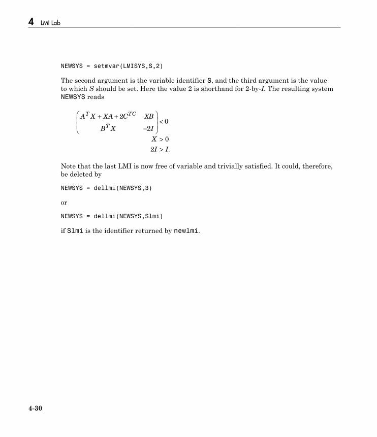
4 LMI Lab
4-30
NEWSYS = setmvar(LMISYS,S,2)
The second argument is the variable identifier S, and the third argument is the valueto which S should be set. Here the value 2 is shorthand for 2-by-I. The resulting systemNEWSYS reads
A X XA C XB
B X I
X
I I
T TC
T
+ +
-
Ê
ËÁÁ
ˆ
¯˜˜
<
>>
2
2
0
0
2 .
Note that the last LMI is now free of variable and trivially satisfied. It could, therefore,be deleted by
NEWSYS = dellmi(NEWSYS,3)
or
NEWSYS = dellmi(NEWSYS,Slmi)
if Slmi is the identifier returned by newlmi.
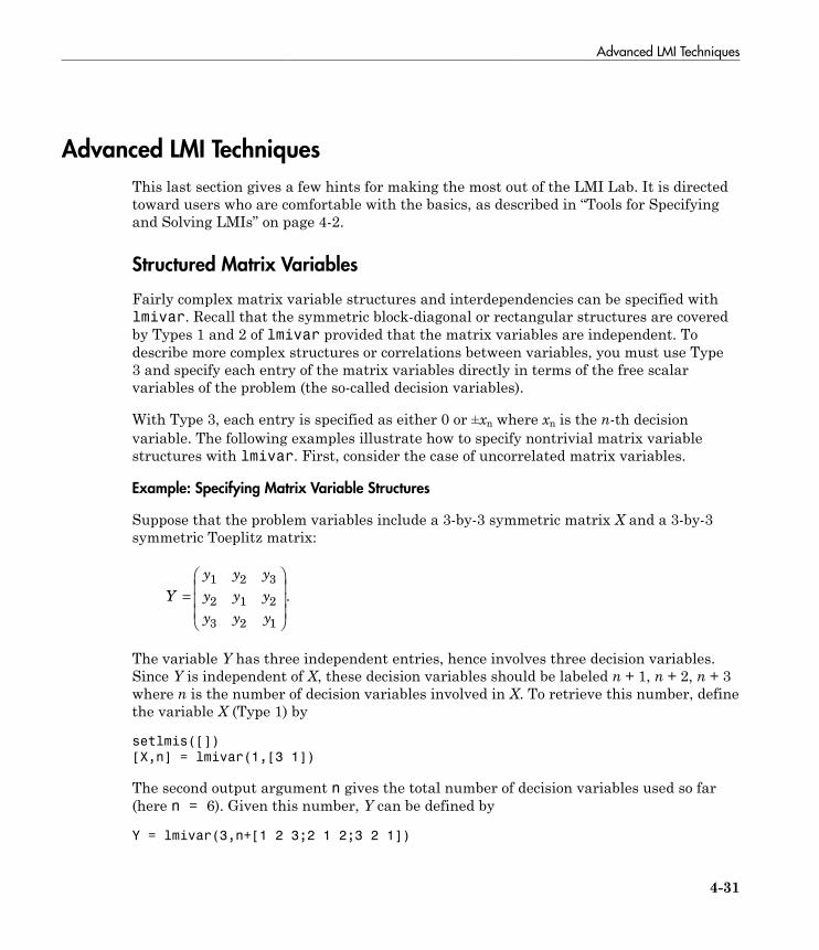
Advanced LMI Techniques
4-31
Advanced LMI Techniques
This last section gives a few hints for making the most out of the LMI Lab. It is directedtoward users who are comfortable with the basics, as described in “Tools for Specifyingand Solving LMIs” on page 4-2.
Structured Matrix Variables
Fairly complex matrix variable structures and interdependencies can be specified withlmivar. Recall that the symmetric block-diagonal or rectangular structures are coveredby Types 1 and 2 of lmivar provided that the matrix variables are independent. Todescribe more complex structures or correlations between variables, you must use Type3 and specify each entry of the matrix variables directly in terms of the free scalarvariables of the problem (the so-called decision variables).
With Type 3, each entry is specified as either 0 or ±xn where xn is the n-th decisionvariable. The following examples illustrate how to specify nontrivial matrix variablestructures with lmivar. First, consider the case of uncorrelated matrix variables.
Example: Specifying Matrix Variable Structures
Suppose that the problem variables include a 3-by-3 symmetric matrix X and a 3-by-3symmetric Toeplitz matrix:
Y
y y y
y y y
y y y
=Ê
Ë
ÁÁÁ
ˆ
¯
˜˜˜
1 2 3
2 1 2
3 2 1
.
The variable Y has three independent entries, hence involves three decision variables.Since Y is independent of X, these decision variables should be labeled n + 1, n + 2, n + 3where n is the number of decision variables involved in X. To retrieve this number, definethe variable X (Type 1) by
setlmis([])
[X,n] = lmivar(1,[3 1])
The second output argument n gives the total number of decision variables used so far(here n = 6). Given this number, Y can be defined by
Y = lmivar(3,n+[1 2 3;2 1 2;3 2 1])
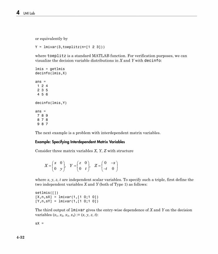
4 LMI Lab
4-32
or equivalently by
Y = lmivar(3,toeplitz(n+[1 2 3]))
where toeplitz is a standard MATLAB function. For verification purposes, we canvisualize the decision variable distributions in X and Y with decinfo:
lmis = getlmis
decinfo(lmis,X)
ans =
1 2 4
2 3 5
4 5 6
decinfo(lmis,Y)
ans =
7 8 9
8 7 8
9 8 7
The next example is a problem with interdependent matrix variables.
Example: Specifying Interdependent Matrix Variables
Consider three matrix variables X, Y, Z with structure
Xx
yY
z
tZ
x
t=
Ê
ËÁ
ˆ
¯˜ =
Ê
ËÁ
ˆ
¯˜ =
--
Ê
ËÁ
ˆ
¯˜
0
0
0
0
0
0, ,
where x, y, z, t are independent scalar variables. To specify such a triple, first define thetwo independent variables X and Y (both of Type 1) as follows:
setlmis([])
[X,n,sX] = lmivar(1,[1 0;1 0])
[Y,n,sY] = lmivar(1,[1 0;1 0])
The third output of lmivar gives the entry-wise dependence of X and Y on the decisionvariables (x1, x2, x3, x4) := (x, y, z, t):
sX =

Advanced LMI Techniques
4-33
1 0
0 2
sY =
3 0
0 4
Using Type 3 of lmivar, you can now specify the structure of Z in terms of the decisionvariables x1 = x and x4 = t:
[Z,n,sZ] = lmivar(3,[0 –sX(1,1);–sY(2,2) 0])
Since sX(1,1) refers to x1 while sY(2,2) refers to x4, this defines the variable
Zx
x
x
t=
--
Ê
ËÁ
ˆ
¯˜ =
--
Ê
ËÁ
ˆ
¯˜
0
0
0
0
1
4
as confirmed by checking its entry-wise dependence on the decision variables:
sZ =
0 –1
–4 0
Complex-Valued LMIs
The LMI solvers are written for real-valued matrices and cannot directly handle LMIproblems involving complex-valued matrices. However, complex-valued LMIs can beturned into real-valued LMIs by observing that a complex Hermitian matrix L(x) satisfies
L(x) < 0
if and only if
Re Im
Im Re.
L x L x
L x L x
( )( ) ( )( )- ( )( ) ( )( )
Ê
ËÁÁ
ˆ
¯˜˜ < 0
This suggests the following systematic procedure for turning complex LMIs into realones:

4 LMI Lab
4-34
• Decompose every complex matrix variable X as
X = X1 + jX2
where X1 and X2 are real• Decompose every complex matrix coefficient A as
A = A1 + jA2
where A1 and A2 are real• Carry out all complex matrix products. This yields affine expressions in X1, X2 for the
real and imaginary parts of each LMI, and an equivalent real-valued LMI is readilyderived from the above observation.
For LMIs without outer factor, a streamlined version of this procedure consists ofreplacing any occurrence of the matrix variable X = X1 + jX2 by
X X
X X
1 2
2 1-
Ê
ËÁ
ˆ
¯˜
and any fixed matrix A = A1 + jA2, including real ones, by
A A
A A
1 2
2 1-
Ê
ËÁ
ˆ
¯˜.
For instance, the real counterpart of the LMI system
MHXM < X, X = XH > I
reads (given the decompositions M = M1 + jM2 and X = X1 + jX2 with Mj, Xj real):
M M
M M
X X
X X
M M
M M
X X
X X
T
1 2
2 1
1 2
2 1
1 2
2 1
1 2
2 1-Ê
ËÁ
ˆ
¯˜ -
Ê
ËÁ
ˆ
¯˜ -Ê
ËÁ
ˆ
¯˜ <
-Ê
ËÁÁ
ˆ
¯˜
-Ê
ËÁ
ˆ
¯˜ <
X X
X XI
1 2
2 1
.
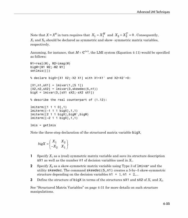
Advanced LMI Techniques
4-35
Note that X = XH in turn requires that X XH
1 1= and X X
T
2 20+ = . Consequently,
X1 and X2 should be declared as symmetric and skew- symmetric matrix variables,respectively.
Assuming, for instance, that M ∊ C5×5, the LMI system (Equation 4-11) would be specifiedas follows:
M1=real(M), M2=imag(M)
bigM=[M1 M2;-M2 M1]
setlmis([])
% declare bigX=[X1 X2;-X2 X1] with X1=X1' and X2+X2'=0:
[X1,n1,sX1] = lmivar(1,[5 1])
[X2,n2,sX2] = lmivar(3,skewdec(5,n1))
bigX = lmivar(3,[sX1 sX2;-sX2 sX1])
% describe the real counterpart of (1.12):
lmiterm([1 1 1 0],1)
lmiterm([–1 1 1 bigX],1,1)
lmiterm([2 1 1 bigX],bigM',bigM)
lmiterm([–2 1 1 bigX],1,1)
lmis = getlmis
Note the three-step declaration of the structured matrix variable bigX,
bigXX X
X X=
-Ê
ËÁ
ˆ
¯˜
1 2
2 1
.
1 Specify X1 as a (real) symmetric matrix variable and save its structure descriptionsX1 as well as the number n1 of decision variables used in X1.
2 Specify X2 as a skew-symmetric matrix variable using Type 3 of lmivar and theutility skewdec. The command skewdec(5,n1) creates a 5-by–5 skew-symmetricstructure depending on the decision variables n1 + 1, n1 + 2,...
3 Define the structure of bigX in terms of the structures sX1 and sX2 of X1 and X2.
See “Structured Matrix Variables” on page 4-31 for more details on such structuremanipulations.

4 LMI Lab
4-36
Specifying cTx Objectives for mincx
The LMI solver mincx minimizes linear objectives of the form cTx where x is the vectorof decision variables. In most control problems, however, such objectives are expressed interms of the matrix variables rather than of x. Examples include Trace(X) where X is asymmetric matrix variable, or uTXu where u is a given vector.
The function defcx facilitates the derivation of the c vector when the objective is anaffine function of the matrix variables. For the sake of illustration, consider the linearobjective
Trace X x PxT( ) +0 0
where X and P are two symmetric variables and x0 is a given vector. If lmsisys is theinternal representation of the LMI system and if x0, X, P have been declared by
x0 = [1;1]
setlmis([])
X = lmivar(1,[3 0])
P = lmivar(1,[2 1])
:
:
lmisys = getlmis
the c vector such that c x X x PxT T
= ( ) +Trace0 0
can be computed as follows:
n = decnbr(lmisys)
c = zeros(n,1)
for j=1:n,
[Xj,Pj] = defcx(lmisys,j,X,P)
c(j) = trace(Xj) + x0'*Pj*x0
end
The first command returns the number of decision variables in the problem and thesecond command dimensions c accordingly. Then the for loop performs the followingoperations:
1 Evaluate the matrix variables X and P when all entries of the decision vector x areset to zero except xj: = 1. This operation is performed by the function defcx. Apart

Advanced LMI Techniques
4-37
from lmisys and j, the inputs of defcx are the identifiers X and P of the variablesinvolved in the objective, and the outputs Xj and Pj are the corresponding values.
2 Evaluate the objective expression for X:= Xj and P:= Pj. This yields the j-th entryof c by definition.
In our example the result is
c =
3
1
2
1
Other objectives are handled similarly by editing the following generic skeleton:
n = decnbr( LMI system )
c = zeros(n,1)
for j=1:n,
[ matrix values ] = defcx( LMI system,j,
matrix identifiers)
c(j) = objective(matrix values)
end
Feasibility Radius
When solving LMI problems with feasp, mincx, or gevp, it is possible to constrain thesolution x to lie in the ball
xTx < R2
where R > 0 is called the feasibility radius. This specifies a maximum (Euclidean norm)magnitude for x and avoids getting solutions of very large norm. This may also speedup computations and improve numerical stability. Finally, the feasibility radius boundregularizes problems with redundant variable sets. In rough terms, the set of scalarvariables is redundant when an equivalent problem could be formulated with a smallernumber of variables.
The feasibility radius R is set by the third entry of the options vector of the LMI solvers.Its default value is R = 109. Setting R to a negative value means “no rigid bound,” inwhich case the feasibility radius is increased during the optimization if necessary. This“flexible bound” mode may yield solutions of large norms.

4 LMI Lab
4-38
Well-Posedness Issues
The LMI solvers used in the LMI Lab are based on interior-point optimizationtechniques. To compute feasible solutions, such techniques require that the system ofLMI constraints be strictly feasible, that is, the feasible set has a nonempty interior. As aresult, these solvers may encounter difficulty when the LMI constraints are feasible butnot strictly feasible, that is, when the LMI
L(x) ≤ 0
has solutions while
L(x) < 0
has no solution.
For feasibility problems, this difficulty is automatically circumvented by feasp, whichreformulates the problem:
Find x such that
L(x) ≤ 0
as:
Minimize t subject to
Lx < t × I.
In this modified problem, the LMI constraint is always strictly feasible in x, t andthe original LMI Equation 4-12 is feasible if and only if the global minimum tmin ofEquation 4-12 satisfies
tmin ≤ 0
For feasible but not strictly feasible problems, however, the computational effort istypically higher as feasp strives to approach the global optimum tmin = 0 to a highaccuracy.
For the LMI problems addressed by mincx and gevp, nonstrict feasibility generallycauses the solvers to fail and to return an “infeasibility” diagnosis. Although there is
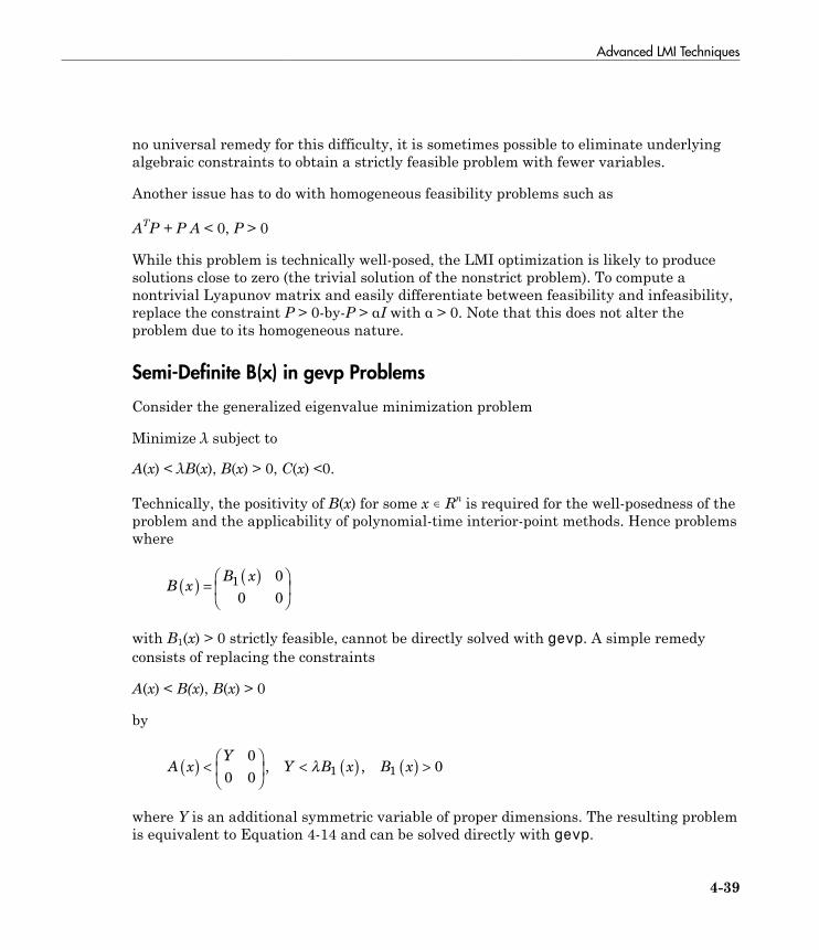
Advanced LMI Techniques
4-39
no universal remedy for this difficulty, it is sometimes possible to eliminate underlyingalgebraic constraints to obtain a strictly feasible problem with fewer variables.
Another issue has to do with homogeneous feasibility problems such as
ATP + P A < 0, P > 0
While this problem is technically well-posed, the LMI optimization is likely to producesolutions close to zero (the trivial solution of the nonstrict problem). To compute anontrivial Lyapunov matrix and easily differentiate between feasibility and infeasibility,replace the constraint P > 0-by-P > αI with α > 0. Note that this does not alter theproblem due to its homogeneous nature.
Semi-Definite B(x) in gevp Problems
Consider the generalized eigenvalue minimization problem
Minimize λ subject to
A(x) < λB(x), B(x) > 0, C(x) <0.
Technically, the positivity of B(x) for some x ∊ Rn is required for the well-posedness of theproblem and the applicability of polynomial-time interior-point methods. Hence problemswhere
B xB x( ) = ( )Ê
ËÁ
ˆ
¯˜1
0
0 0
with B1(x) > 0 strictly feasible, cannot be directly solved with gevp. A simple remedyconsists of replacing the constraints
A(x) < B(x), B(x) > 0
by
A xY
Y B x B x( ) <Ê
ËÁ
ˆ
¯˜ < ( ) ( ) >
0
0 001 1, ,l
where Y is an additional symmetric variable of proper dimensions. The resulting problemis equivalent to Equation 4-14 and can be solved directly with gevp.
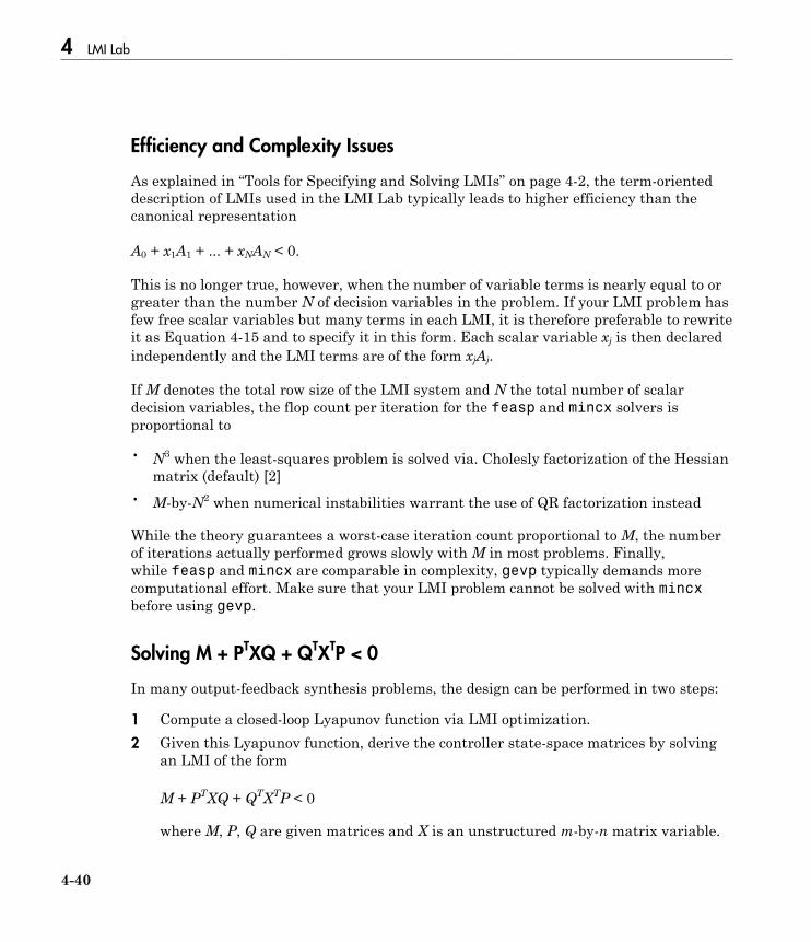
4 LMI Lab
4-40
Efficiency and Complexity Issues
As explained in “Tools for Specifying and Solving LMIs” on page 4-2, the term-orienteddescription of LMIs used in the LMI Lab typically leads to higher efficiency than thecanonical representation
A0 + x1A1 + ... + xNAN < 0.
This is no longer true, however, when the number of variable terms is nearly equal to orgreater than the number N of decision variables in the problem. If your LMI problem hasfew free scalar variables but many terms in each LMI, it is therefore preferable to rewriteit as Equation 4-15 and to specify it in this form. Each scalar variable xj is then declaredindependently and the LMI terms are of the form xjAj.
If M denotes the total row size of the LMI system and N the total number of scalardecision variables, the flop count per iteration for the feasp and mincx solvers isproportional to
• N3 when the least-squares problem is solved via. Cholesly factorization of the Hessianmatrix (default) [2]
• M-by-N2 when numerical instabilities warrant the use of QR factorization instead
While the theory guarantees a worst-case iteration count proportional to M, the numberof iterations actually performed grows slowly with M in most problems. Finally,while feasp and mincx are comparable in complexity, gevp typically demands morecomputational effort. Make sure that your LMI problem cannot be solved with mincxbefore using gevp.
Solving M + PTXQ + QTXTP < 0
In many output-feedback synthesis problems, the design can be performed in two steps:
1 Compute a closed-loop Lyapunov function via LMI optimization.2 Given this Lyapunov function, derive the controller state-space matrices by solving
an LMI of the form
M + PTXQ + QTXTP < 0
where M, P, Q are given matrices and X is an unstructured m-by-n matrix variable.

Advanced LMI Techniques
4-41
It turns out that a particular solution Xc of Equation 4-16 can be computed via simplelinear algebra manipulations [1]. Typically, Xc corresponds to the center of the ellipsoidof matrices defined by Equation 4-16.
The function basiclmi returns the “explicit” solution Xc:
Xc = basiclmi(M,P,Q)
Since this central solution sometimes has large norm, basiclmi also offers the option ofcomputing an approximate least-norm solution of Equation 4-16. This is done by
X = basiclmi(M,P,Q,'Xmin')
and involves LMI optimization to minimize ∥X ∥.

4 LMI Lab
4-42
Bibliography
[1] Gahinet, P., and P. Apkarian, “A Linear Matrix Inequality Approach to H∞ Control,”Int. J. Robust and Nonlinear Contr., 4 (1994), pp. 421-448.
[2] Nemirovski, A., and P. Gahinet, “The Projective Method for Solving Linear MatrixInequalities,” Proc. Amer. Contr. Conf., 1994, pp. 840-844.
[3] Nesterov, Yu, and A. Nemirovski, Interior Point Polynomial Methods in ConvexProgramming: Theory and Applications, SIAM Books, Philadelphia, 1994.
[4] Shamma, J.S., “Robustness Analysis for Time-Varying Systems,” Proc. Conf. Dec.Contr., 1992, pp. 3163-3168.
5
Analyzing Uncertainty Effects inSimulink
• “Analyzing Uncertainty in Simulink” on page 5-2• “Simulink Blocks for Analyzing Uncertainty” on page 5-3• “Specify Uncertainty Using Uncertain State Space Blocks” on page 5-4• “Simulate Uncertainty Effects” on page 5-7• “Vary Uncertainty Values Using Individual Uncertain State Space Blocks” on page
5-8• “Vary Uncertainty Values Across Multiple Uncertain State Space Blocks” on page
5-14• “Computing Uncertain State-Space Models from Simulink Models” on page 5-19• “Obtain Uncertain State-Space Model from Simulink Model” on page 5-20• “Specify Uncertain Linearization for Core or Custom Simulink Blocks” on page
5-21• “Linearize Block to Uncertain Model” on page 5-24• “Using Uncertain Linearization for Analysis or Control Design” on page 5-26• “Analyzing Stability Margin of Simulink Models” on page 5-27• “Stability Margin of a Simulink Model” on page 5-29
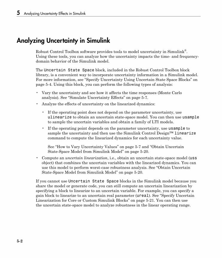
5 Analyzing Uncertainty Effects in Simulink
5-2
Analyzing Uncertainty in Simulink
Robust Control Toolbox software provides tools to model uncertainty in Simulink®.Using these tools, you can analyze how the uncertainty impacts the time- and frequency-domain behavior of the Simulink model.
The Uncertain State Space block, included in the Robust Control Toolbox blocklibrary, is a convenient way to incorporate uncertainty information in a Simulink model.For more information, see “Specify Uncertainty Using Uncertain State Space Blocks” onpage 5-4. Using this block, you can perform the following types of analysis:
• Vary the uncertainty and see how it affects the time responses (Monte Carloanalysis). See “Simulate Uncertainty Effects” on page 5-7.
• Analyze the effects of uncertainty on the linearized dynamics:
• If the operating point does not depend on the parameter uncertainty, useulinearize to obtain an uncertain state-space model. You can then use usampleto sample the uncertain variables and obtain a family of LTI models.
• If the operating point depends on the parameter uncertainty, use usample tosample the uncertainty and then use the Simulink Control Design™ linearizecommand to compute the linearized dynamics for each uncertainty value.
See “How to Vary Uncertainty Values” on page 5-7 and “Obtain UncertainState-Space Model from Simulink Model” on page 5-20.
• Compute an uncertain linearization, i.e., obtain an uncertain state-space model (ussobject) that combines the uncertain variables with the linearized dynamics. You canuse this model to perform worst-case robustness analysis. See “Obtain UncertainState-Space Model from Simulink Model” on page 5-20.
If you cannot use Uncertain State Space blocks in the Simulink model because youshare the model or generate code, you can still compute an uncertain linearization byspecifying a block to linearize to an uncertain variable. For example, you can specify again block to linearize to an uncertain real parameter (ureal). See “Specify UncertainLinearization for Core or Custom Simulink Blocks” on page 5-21. You can then usethe uncertain state-space model to analyze robustness in the linear operating range.
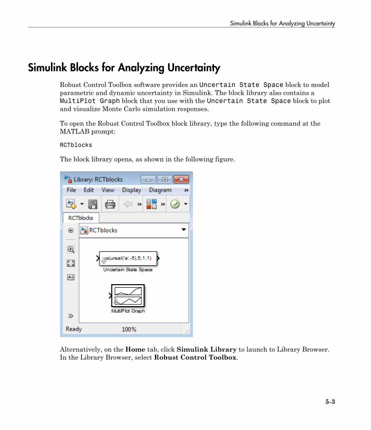
Simulink Blocks for Analyzing Uncertainty
5-3
Simulink Blocks for Analyzing Uncertainty
Robust Control Toolbox software provides an Uncertain State Space block to modelparametric and dynamic uncertainty in Simulink. The block library also contains aMultiPlot Graph block that you use with the Uncertain State Space block to plotand visualize Monte Carlo simulation responses.
To open the Robust Control Toolbox block library, type the following command at theMATLAB prompt:
RCTblocks
The block library opens, as shown in the following figure.
Alternatively, on the Home tab, click Simulink Library to launch to Library Browser.In the Library Browser, select Robust Control Toolbox.

5 Analyzing Uncertainty Effects in Simulink
5-4
Specify Uncertainty Using Uncertain State Space Blocks
• “How to Specify Uncertainty in Uncertain State Space Blocks” on page 5-4• “Next Steps” on page 5-6
How to Specify Uncertainty in Uncertain State Space Blocks
Specifying uncertainty in the Uncertain State Space block makes the uncertaintya part of the Simulink model and affects both simulation and linearization. Use thisapproach to vary the uncertainty and analyze the effects on simulation or linearization.
To specify uncertainty in the Uncertain State Space block:
1 Drag and drop an Uncertain State Space block from the Robust Control Toolboxblock library into a Simulink model. For more information on how to open the blocklibrary, see “Simulink Blocks for Analyzing Uncertainty” on page 5-3.
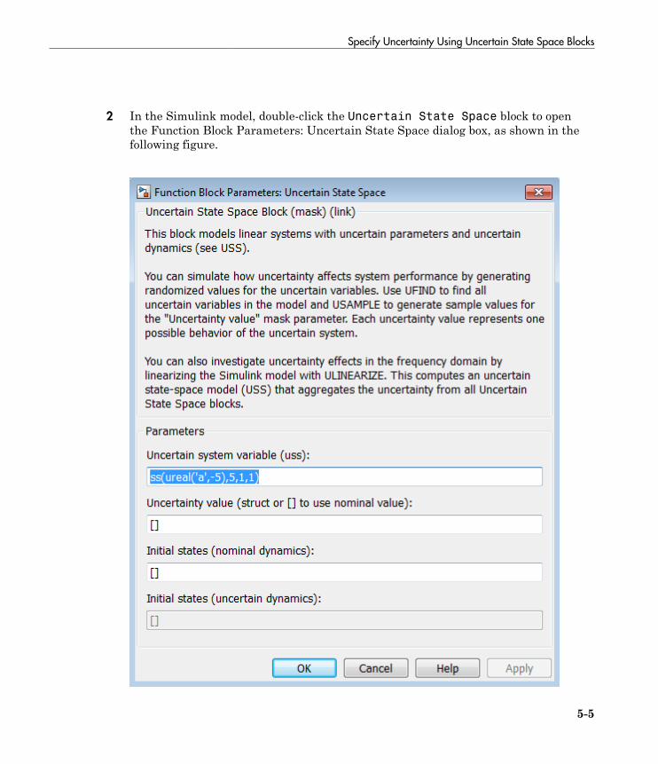
Specify Uncertainty Using Uncertain State Space Blocks
5-5
2 In the Simulink model, double-click the Uncertain State Space block to openthe Function Block Parameters: Uncertain State Space dialog box, as shown in thefollowing figure.
5 Analyzing Uncertainty Effects in Simulink
5-6
3 Specify an uncertain state-space model in the Uncertain system variable (uss)field. The model must be an uss object or any other model that can be converted touss, such as umat, ureal and ultidyn. The model depends on a set of uncertainvariables (ureal or ultidyn) and you can specify the model as one of the following:
• Function or expression that evaluates to an uss model. For example,ss(ureal('a',-5),5,1,1).
• Variable, defined in the MATLAB workspace. For example, unc_sys, whereunc_sys is defined as ss(ureal('a',-5),5,1,1) in the workspace.
4 Specify values for the uncertain variables that the uncertain state-space modelyou specify in step 3 uses. For example, if you specify the uncertain system asureal('g',2)*tf(1,[ureal('tau'),1]), then you must specify values for theuncertain variables g and tau. To do so, enter a structure with fields g and tau inthe Uncertainty value (struct or [] to use nominal value) field. You can alsoenter [] to use the nominal values of the uncertain parameters g and tau.
Tip: You can also use this field to vary the uncertainty values for performing MonteCarlo simulation. For more information, see “Simulate Uncertainty Effects” on page5-7.
5 (Optional) Specify the initial states of the nominal and uncertain dynamics in theInitial states (nominal dynamics) and Initial states (uncertain dynamics)fields, respectively.
For more information on the block parameters, see the Uncertain State Space blockreference page.
Next Steps
After you specify uncertainty in Uncertain State Space blocks, you can perform oneof the following:
• Simulate the model using nominal, manually-defined or random values, as describedin “Simulate Uncertainty Effects” on page 5-7.
• Perform an uncertain linearization, as described in “Obtain Uncertain State-SpaceModel from Simulink Model” on page 5-20.
Simulate Uncertainty Effects
5-7
Simulate Uncertainty Effects
• “How to Simulate Effects of Uncertainty” on page 5-7• “How to Vary Uncertainty Values” on page 5-7
How to Simulate Effects of Uncertainty
As described in “Specify Uncertainty Using Uncertain State Space Blocks” on page 5-4,the uncertain state-space model you specify in the Uncertain State Space blockdepends on a set of uncertain variables (ureal or ultidyn objects.) You can simulatethe model using nominal value of these uncertain variables. Additionally, you can samplethese uncertain variables and simulate the model for various values in the uncertaintyrange (Monte Carlo simulation.) For more information, see “How to Vary UncertaintyValues” on page 5-7. You can view and compare the simulation results for varioussample values of uncertainty using the MultiPlot Graph block.
How to Vary Uncertainty Values
There are two ways to control the uncertainty values using the Uncertainty value(struct or [] to use nominal value) field of the Uncertain State Space blockparameters dialog box:
• For simple models with few uncertain variables or one Uncertain State Spaceblock, type the value in the Uncertain State Space block itself. For moreinformation, see “Vary Uncertainty Values Using Individual Uncertain State SpaceBlocks” on page 5-8.
• For complex models with large number of uncertain variables or Uncertain StateSpace blocks, use a single data structure for all uncertain variables referenced by themodel. Using this approach, you can collectively control the values of all or a subsetof uncertain variables and toggle between nominal and user-defined values fromthe MATLAB prompt. For more information, see “Vary Uncertainty Values AcrossMultiple Uncertain State Space Blocks” on page 5-14.
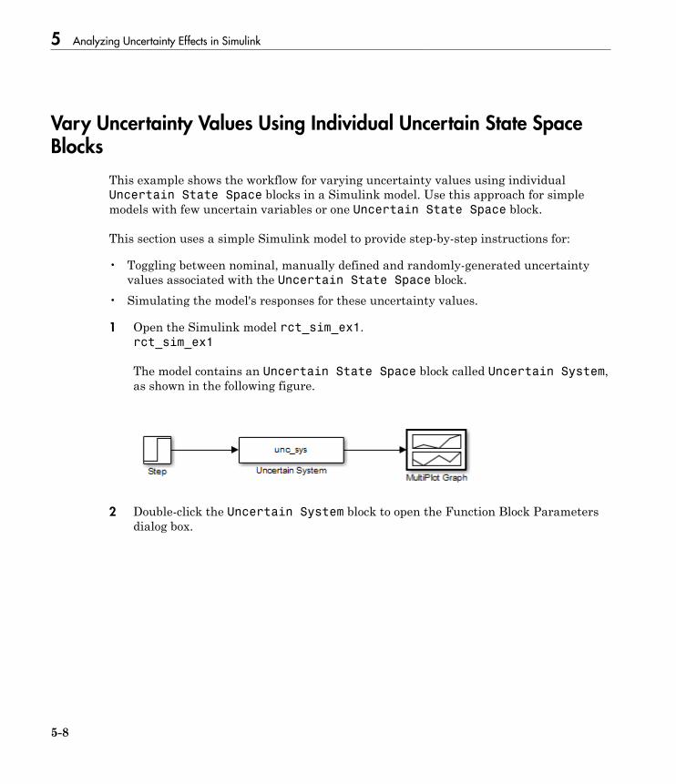
5 Analyzing Uncertainty Effects in Simulink
5-8
Vary Uncertainty Values Using Individual Uncertain State SpaceBlocks
This example shows the workflow for varying uncertainty values using individualUncertain State Space blocks in a Simulink model. Use this approach for simplemodels with few uncertain variables or one Uncertain State Space block.
This section uses a simple Simulink model to provide step-by-step instructions for:
• Toggling between nominal, manually defined and randomly-generated uncertaintyvalues associated with the Uncertain State Space block.
• Simulating the model's responses for these uncertainty values.
1 Open the Simulink model rct_sim_ex1.rct_sim_ex1
The model contains an Uncertain State Space block called Uncertain System,as shown in the following figure.
2 Double-click the Uncertain System block to open the Function Block Parametersdialog box.
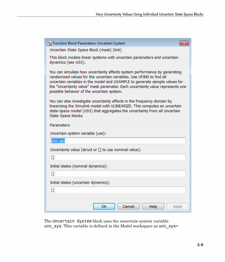
Vary Uncertainty Values Using Individual Uncertain State Space Blocks
5-9
The Uncertain System block uses the uncertain system variableunc_sys. This variable is defined in the Model workspace as unc_sys=
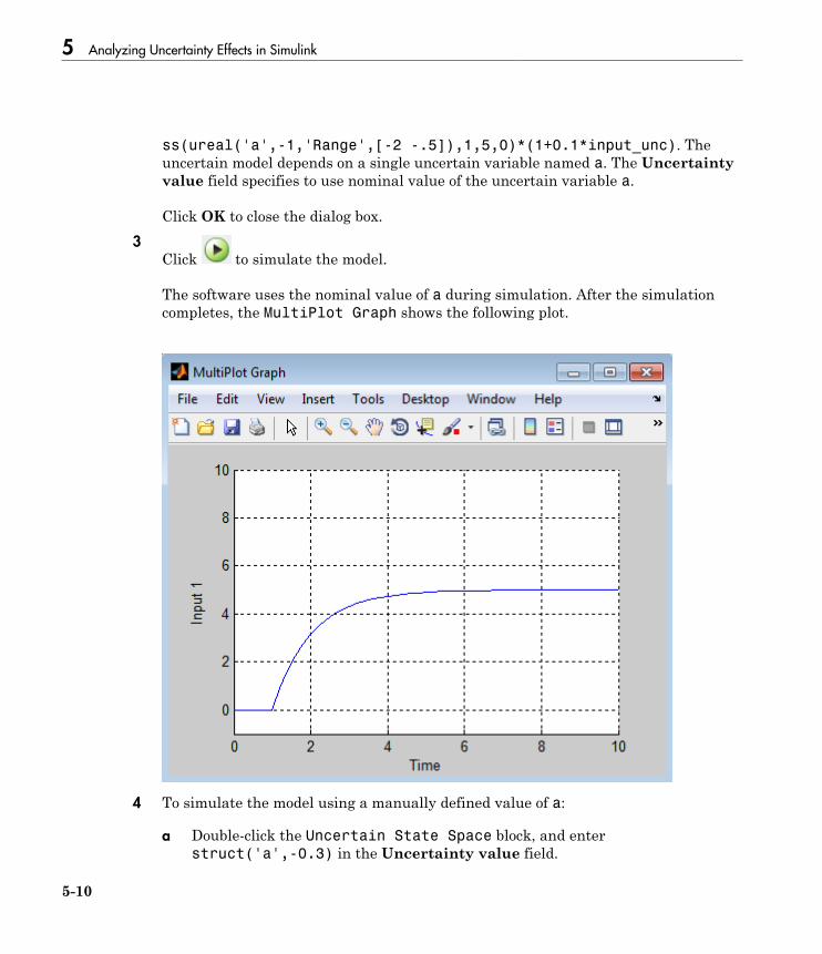
5 Analyzing Uncertainty Effects in Simulink
5-10
ss(ureal('a',-1,'Range',[-2 -.5]),1,5,0)*(1+0.1*input_unc). Theuncertain model depends on a single uncertain variable named a. The Uncertaintyvalue field specifies to use nominal value of the uncertain variable a.
Click OK to close the dialog box.3
Click to simulate the model.
The software uses the nominal value of a during simulation. After the simulationcompletes, the MultiPlot Graph shows the following plot.
4 To simulate the model using a manually defined value of a:
a Double-click the Uncertain State Space block, and enterstruct('a',-0.3) in the Uncertainty value field.
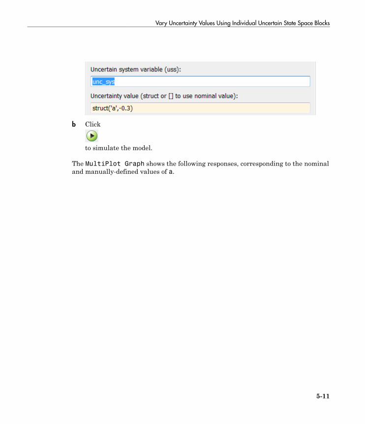
Vary Uncertainty Values Using Individual Uncertain State Space Blocks
5-11
b Click
to simulate the model.
The MultiPlot Graph shows the following responses, corresponding to the nominaland manually-defined values of a.
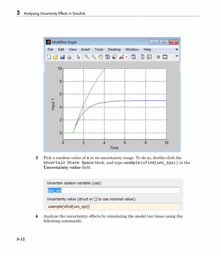
5 Analyzing Uncertainty Effects in Simulink
5-12
5 Pick a random value of a in its uncertainty range. To do so, double-click theUncertain State Space block, and type usample(ufind(unc_sys)) in theUncertainty value field.
6 Analyze the uncertainty effects by simulating the model ten times using thefollowing commands:
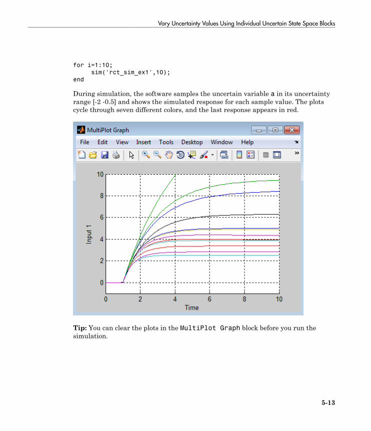
Vary Uncertainty Values Using Individual Uncertain State Space Blocks
5-13
for i=1:10;
sim('rct_sim_ex1',10);
end
During simulation, the software samples the uncertain variable a in its uncertaintyrange [-2 -0.5] and shows the simulated response for each sample value. The plotscycle through seven different colors, and the last response appears in red.
Tip: You can clear the plots in the MultiPlot Graph block before you run thesimulation.
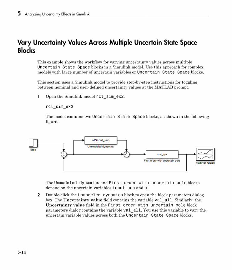
5 Analyzing Uncertainty Effects in Simulink
5-14
Vary Uncertainty Values Across Multiple Uncertain State SpaceBlocks
This example shows the workflow for varying uncertainty values across multipleUncertain State Space blocks in a Simulink model. Use this approach for complexmodels with large number of uncertain variables or Uncertain State Space blocks.
This section uses a Simulink model to provide step-by-step instructions for togglingbetween nominal and user-defined uncertainty values at the MATLAB prompt.
1 Open the Simulink model rct_sim_ex2.
rct_sim_ex2
The model contains two Uncertain State Space blocks, as shown in the followingfigure.
The Unmodeled dynamics and First order with uncertain pole blocksdepend on the uncertain variables input_unc and a.
2 Double-click the Unmodeled dynamics block to open the block parameters dialogbox. The Uncertainty value field contains the variable val_all. Similarly, theUncertainty value field in the First order with uncertain pole blockparameters dialog contains the variable val_all. You use this variable to vary theuncertain variable values across both the Uncertain State Space blocks.
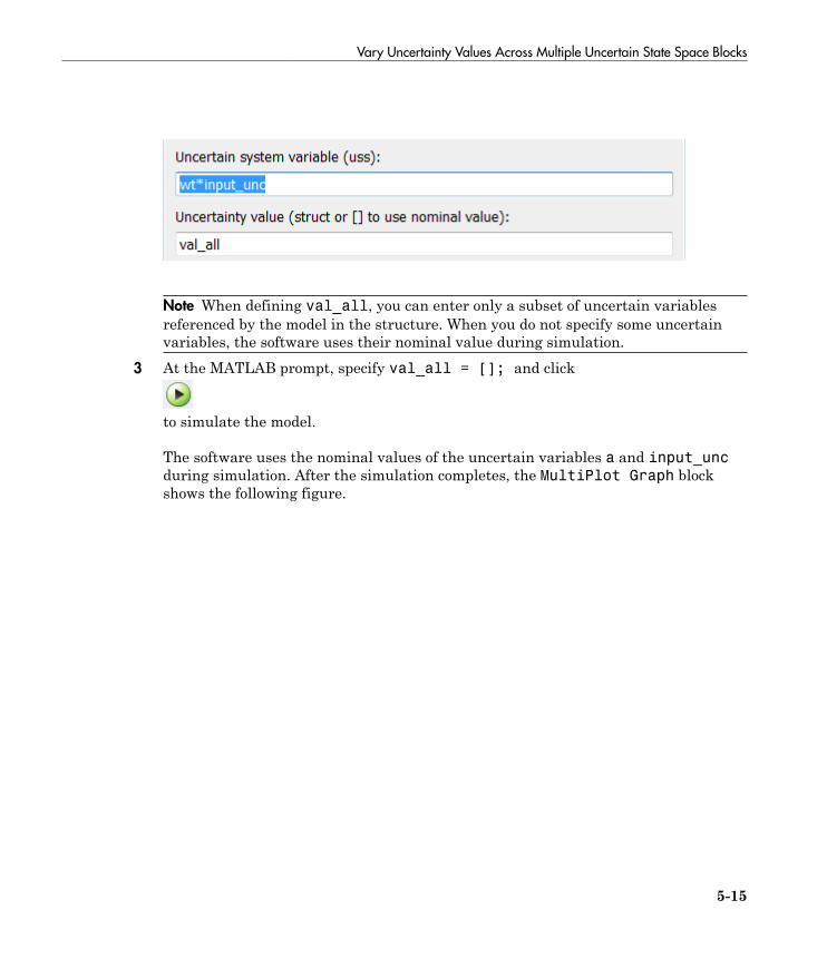
Vary Uncertainty Values Across Multiple Uncertain State Space Blocks
5-15
Note When defining val_all, you can enter only a subset of uncertain variablesreferenced by the model in the structure. When you do not specify some uncertainvariables, the software uses their nominal value during simulation.
3 At the MATLAB prompt, specify val_all = []; and click
to simulate the model.
The software uses the nominal values of the uncertain variables a and input_uncduring simulation. After the simulation completes, the MultiPlot Graph blockshows the following figure.
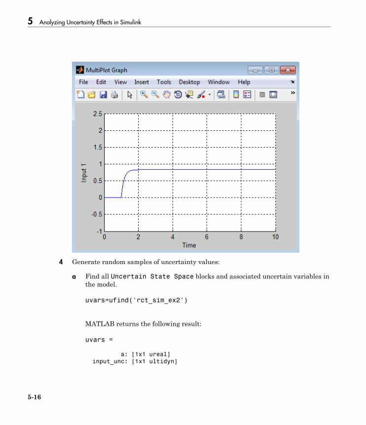
5 Analyzing Uncertainty Effects in Simulink
5-16
4 Generate random samples of uncertainty values:
a Find all Uncertain State Space blocks and associated uncertain variables inthe model.
uvars=ufind('rct_sim_ex2')
MATLAB returns the following result:
uvars =
a: [1x1 ureal]
input_unc: [1x1 ultidyn]
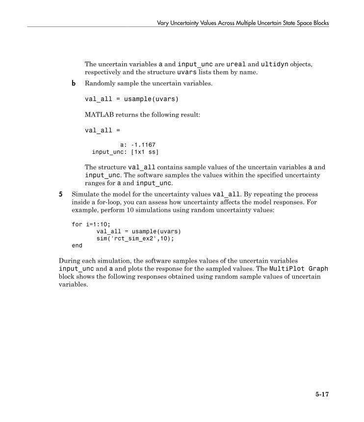
Vary Uncertainty Values Across Multiple Uncertain State Space Blocks
5-17
The uncertain variables a and input_unc are ureal and ultidyn objects,respectively and the structure uvars lists them by name.
b Randomly sample the uncertain variables.
val_all = usample(uvars)
MATLAB returns the following result:
val_all =
a: -1.1167
input_unc: [1x1 ss]
The structure val_all contains sample values of the uncertain variables a andinput_unc. The software samples the values within the specified uncertaintyranges for a and input_unc.
5 Simulate the model for the uncertainty values val_all. By repeating the processinside a for-loop, you can assess how uncertainty affects the model responses. Forexample, perform 10 simulations using random uncertainty values:
for i=1:10;
val_all = usample(uvars)
sim('rct_sim_ex2',10);
end
During each simulation, the software samples values of the uncertain variablesinput_unc and a and plots the response for the sampled values. The MultiPlot Graphblock shows the following responses obtained using random sample values of uncertainvariables.
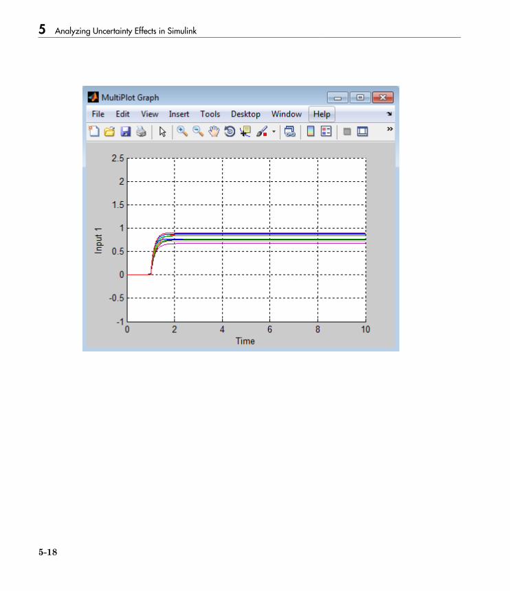
5 Analyzing Uncertainty Effects in Simulink
5-18
Computing Uncertain State-Space Models from Simulink Models
5-19
Computing Uncertain State-Space Models from Simulink Models
When you have the Simulink Control Design software, you can compute an uncertainlinearization, i.e., an uncertain state-space model (uss) combining the uncertainvariables with linearized dynamics. Use the uss model to perform linear analysis androbust control design.
You can compute an uncertain linearization in one of the following ways:
• Using the ulinearize command, as described in “Obtain Uncertain State-SpaceModel from Simulink Model” on page 5-20.
• Using the Simulink Control Design linearize command, as described in “SpecifyUncertain Linearization for Core or Custom Simulink Blocks” on page 5-21.

5 Analyzing Uncertainty Effects in Simulink
5-20
Obtain Uncertain State-Space Model from Simulink Model
To obtain an uncertain state-space model from a model that contains Uncertain StateSpace blocks, use the following steps:
Note If you do not have Uncertain State Space blocks in the model but still want toobtain an uncertain state-space model, see “Specify Uncertain Linearization for Core orCustom Simulink Blocks” on page 5-21.
1 (Prerequisite) Create or open the Simulink model.2 (Prerequisite) In the Simulink model, specify the linearization input and output
points using Simulink Control Design getlinio or linio commands. For moreinformation, see “Specifying Portion of Model to Linearize” in the Simulink ControlDesign documentation.
3 (Prerequisite) If you have not already done so, specify uncertainty in the Simulinkmodel as described in “Specify Uncertainty Using Uncertain State Space Blocks” onpage 5-4.
Note The software does not evaluate the uncertain variables during linearization.Thus, the value of the uncertainty does not affect the linearization.
4 Run ulinearize to compute an uncertain linearization. This command returns anuss model.
Note If you use the Simulink Control Designlinearize command, the UncertainState Space blocks linearize to their nominal value.
For more information on linearization and how to evaluate the results, see “LinearizationBasics” in the Simulink Control Design documentation.
For an example of how to use the Simulink Control Design linearize command, seeLinearization of Simulink Models with Uncertainty.
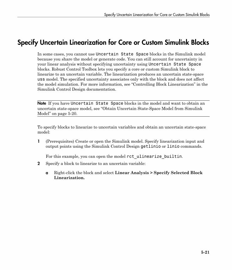
Specify Uncertain Linearization for Core or Custom Simulink Blocks
5-21
Specify Uncertain Linearization for Core or Custom Simulink Blocks
In some cases, you cannot use Uncertain State Space blocks in the Simulink modelbecause you share the model or generate code. You can still account for uncertainty inyour linear analysis without specifying uncertainty using Uncertain State Spaceblocks. Robust Control Toolbox lets you specify a core or custom Simulink block tolinearize to an uncertain variable. The linearization produces an uncertain state-spaceuss model. The specified uncertainty associates only with the block and does not affectthe model simulation. For more information, see “Controlling Block Linearization” in theSimulink Control Design documentation.
Note If you have Uncertain State Space blocks in the model and want to obtain anuncertain state-space model, see “Obtain Uncertain State-Space Model from SimulinkModel” on page 5-20.
To specify blocks to linearize to uncertain variables and obtain an uncertain state-spacemodel:
1 (Prerequisites) Create or open the Simulink model. Specify linearization input andoutput points using the Simulink Control Design getlinio or linio commands.
For this example, you can open the model rct_ulinearize_builtin.2 Specify a block to linearize to an uncertain variable:
a Right-click the block and select Linear Analysis > Specify Selected BlockLinearization.
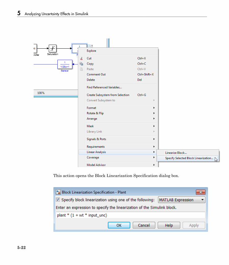
5 Analyzing Uncertainty Effects in Simulink
5-22
This action opens the Block Linearization Specification dialog box.
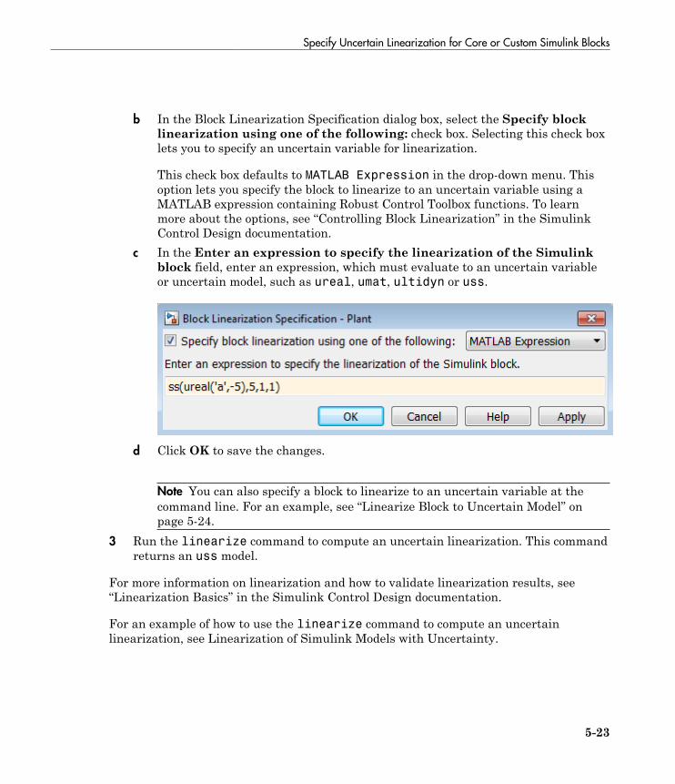
Specify Uncertain Linearization for Core or Custom Simulink Blocks
5-23
b In the Block Linearization Specification dialog box, select the Specify blocklinearization using one of the following: check box. Selecting this check boxlets you to specify an uncertain variable for linearization.
This check box defaults to MATLAB Expression in the drop-down menu. Thisoption lets you specify the block to linearize to an uncertain variable using aMATLAB expression containing Robust Control Toolbox functions. To learnmore about the options, see “Controlling Block Linearization” in the SimulinkControl Design documentation.
c In the Enter an expression to specify the linearization of the Simulinkblock field, enter an expression, which must evaluate to an uncertain variableor uncertain model, such as ureal, umat, ultidyn or uss.
d Click OK to save the changes.
Note You can also specify a block to linearize to an uncertain variable at thecommand line. For an example, see “Linearize Block to Uncertain Model” onpage 5-24.
3 Run the linearize command to compute an uncertain linearization. This commandreturns an uss model.
For more information on linearization and how to validate linearization results, see“Linearization Basics” in the Simulink Control Design documentation.
For an example of how to use the linearize command to compute an uncertainlinearization, see Linearization of Simulink Models with Uncertainty.
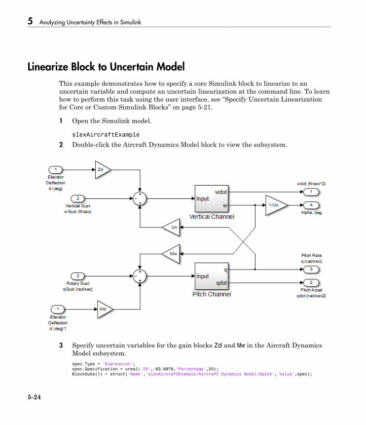
5 Analyzing Uncertainty Effects in Simulink
5-24
Linearize Block to Uncertain Model
This example demonstrates how to specify a core Simulink block to linearize to anuncertain variable and compute an uncertain linearization at the command line. To learnhow to perform this task using the user interface, see “Specify Uncertain Linearizationfor Core or Custom Simulink Blocks” on page 5-21.
1 Open the Simulink model.
slexAircraftExample
2 Double-click the Aircraft Dynamics Model block to view the subsystem.
3 Specify uncertain variables for the gain blocks Zd and Mw in the Aircraft DynamicsModel subsystem.spec.Type = 'Expression';
spec.Specification = ureal('Zd',-63.9979,'Percentage',20);
BlockSubs(1) = struct('Name','slexAircraftExample/Aircraft Dynamics Model/Gain5','Value',spec);
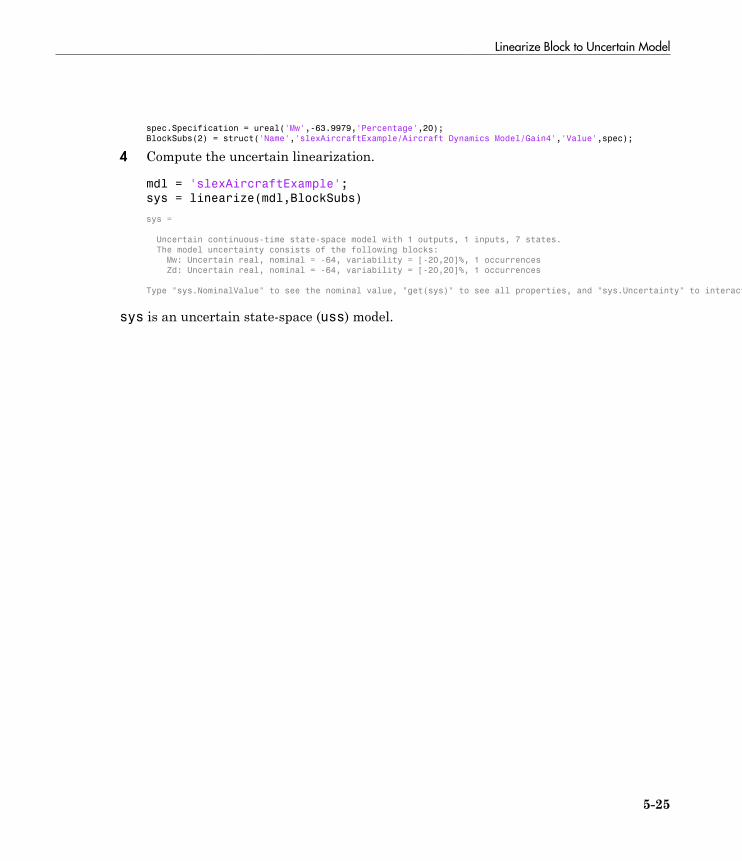
Linearize Block to Uncertain Model
5-25
spec.Specification = ureal('Mw',-63.9979,'Percentage',20);
BlockSubs(2) = struct('Name','slexAircraftExample/Aircraft Dynamics Model/Gain4','Value',spec);
4 Compute the uncertain linearization.
mdl = 'slexAircraftExample';
sys = linearize(mdl,BlockSubs)
sys =
Uncertain continuous-time state-space model with 1 outputs, 1 inputs, 7 states.
The model uncertainty consists of the following blocks:
Mw: Uncertain real, nominal = -64, variability = [-20,20]%, 1 occurrences
Zd: Uncertain real, nominal = -64, variability = [-20,20]%, 1 occurrences
Type "sys.NominalValue" to see the nominal value, "get(sys)" to see all properties, and "sys.Uncertainty" to interact with the uncertain elements.
sys is an uncertain state-space (uss) model.
5 Analyzing Uncertainty Effects in Simulink
5-26
Using Uncertain Linearization for Analysis or Control Design
After computing an uncertain linearization, you can perform one of the following:
• Perform robustness analysis.• Perform robust control design.

Analyzing Stability Margin of Simulink Models
5-27
Analyzing Stability Margin of Simulink Models
Robust Control Toolbox provides the loopmargin command to analyze the stabilitymargins of LTI models created in MATLAB and Simulink models. To use loopmarginwith Simulink models, you must have the Simulink Control Design software. Thissection describes the difference between the MATLAB and Simulink approaches of usingloopmargin and the workflow for computing the stability margin of Simulinkmodels.For more information on how to analyze the stability margins of LTI models, see “MIMORobustness Analysis”.
How Stability Margin Analysis Using Loopmargin Differs BetweenSimulink and LTI Models
When analyzing stability margins of LTI models using the syntax [cm,dm,mm] =loopmargin(P,C), the software assumes the input and output of the linear plant P asthe margin analysis points, as shown in the following figure.
Analyzing stability margin of Simulink models differs from analyzing stability margin ofLTI models because you can enter specific margin analysis points in the Simulink model.For more information on how to assign margin analysis points in Simulink models, seethe “Usage with Simulink” section of the loopmargin reference page.
Stability Margin of Simulink Model
The loopmargin command computes the following types of stability margins:
5 Analyzing Uncertainty Effects in Simulink
5-28
• Loop-at-a-time classical gain and phase margins• Loop-at-a-time disk margins• Multi-loop disk margin
To learn more about these stability margins, see the “Algorithms” section of theloopmargin reference page.
The loopmargin command computes the stability margin based on linearization ofSimulink models. To compute stability margins of a Simulink model:
1 Specify the block where you want to define a margin analysis point.2 Specify the output port of the block where you want the margin analysis point.
The software performs the analysis by opening the loop at all specified marginanalysis point.
3 Use the loopmargin command to compute the stability margins at the marginanalysis point.
Optionally, you can compare the classical gain and phase margins obtained usingloopmargin with the stability margins computed for the linearized model. The resultsusing the two approaches should match for simple SISO models. For MIMO models, theloopmargin command provides richer robustness information. For an example, see“Stability Margin of a Simulink Model” on page 5-29.
Additionally, you can compute stability margins by specifying multiple margin analysispoints and multiple operating points. For an example, see Loop Margins for an AirframeAutopilot.
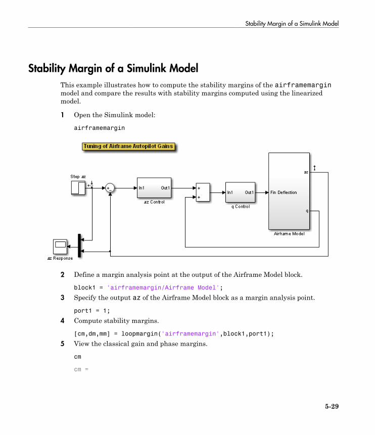
Stability Margin of a Simulink Model
5-29
Stability Margin of a Simulink Model
This example illustrates how to compute the stability margins of the airframemarginmodel and compare the results with stability margins computed using the linearizedmodel.
1 Open the Simulink model:
airframemargin
2 Define a margin analysis point at the output of the Airframe Model block.
block1 = 'airframemargin/Airframe Model';
3 Specify the output az of the Airframe Model block as a margin analysis point.
port1 = 1;
4 Compute stability margins.
[cm,dm,mm] = loopmargin('airframemargin',block1,port1);
5 View the classical gain and phase margins.
cm
cm =
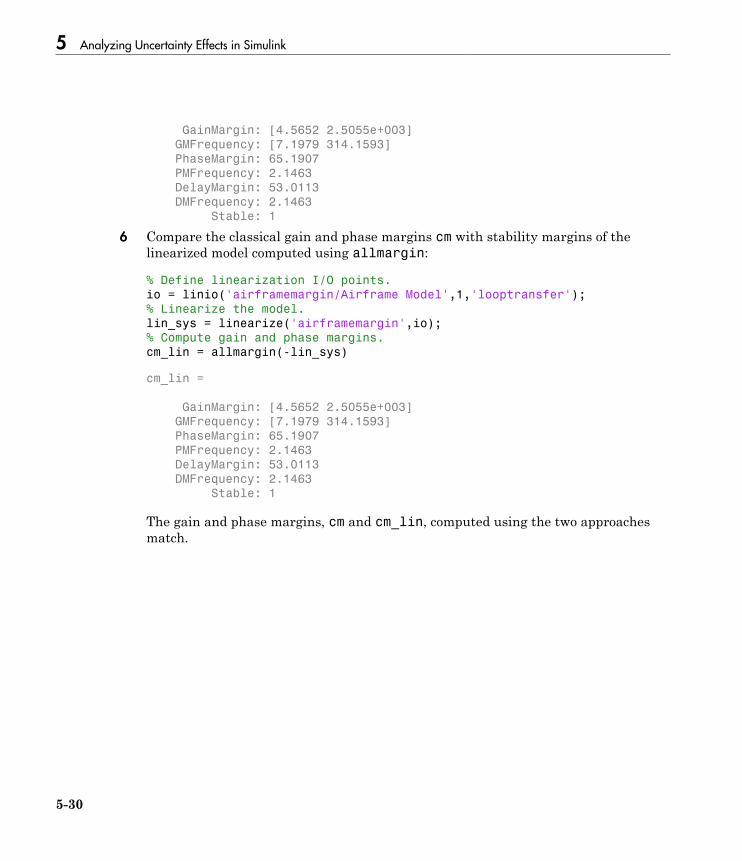
5 Analyzing Uncertainty Effects in Simulink
5-30
GainMargin: [4.5652 2.5055e+003]
GMFrequency: [7.1979 314.1593]
PhaseMargin: 65.1907
PMFrequency: 2.1463
DelayMargin: 53.0113
DMFrequency: 2.1463
Stable: 1
6 Compare the classical gain and phase margins cm with stability margins of thelinearized model computed using allmargin:
% Define linearization I/O points.
io = linio('airframemargin/Airframe Model',1,'looptransfer');
% Linearize the model.
lin_sys = linearize('airframemargin',io);
% Compute gain and phase margins.
cm_lin = allmargin(-lin_sys)
cm_lin =
GainMargin: [4.5652 2.5055e+003]
GMFrequency: [7.1979 314.1593]
PhaseMargin: 65.1907
PMFrequency: 2.1463
DelayMargin: 53.0113
DMFrequency: 2.1463
Stable: 1
The gain and phase margins, cm and cm_lin, computed using the two approachesmatch.