Toolbox of Functional Analysis
76
Appendix A Toolbox of Functional Analysis In this Appendix we provide many definitions and results related to Banach and Hilbert spaces, which form a useful toolbox for the analysis of OCPs governed by PDEs. Further details can be found on, e.g., [237, 52, 274, 65]. A.1 Metric, Banach and Hilbert Spaces A.1.1 Metric Spaces A metric space is a set M endowed with a distance d : M × M → R, satisfying the following three properties, for every x, y, z ∈ M : D 1 : d (x,y) ≥ 0,d (x,y) = 0 if and only if x = y (positivity ) D 2 : d (x,y)= d (y,x) (symmetry ) D 3 : d (x,z) ≤ d (x,y)+ d (y,z) (triangular inequality ). A metric space does not need to be a linear (vector) space. A sequence {x n }⊂ M converges to x in M , and we write x m → x in M , if d (x m ,x) → 0 as m →∞. The limit is unique: if d (x m ,x) → 0 and d (x m ,y) → 0 as m →∞, then, from the triangular inequality, we have d (x,y) ≤ d (x m ,x)+ d (x m ,y) → 0 as m →∞ which implies x = y. We call B r (x)= {y ∈ M : d (x,y) <r} the open ball of radius r, centered at x. As in the finite dimensional space R d , we can define a topology in M , induced by the metric. Let A ⊆ M ; a point x ∈ A is: • an interior point if there exists a ball B r (x) ⊂ A; • a boundary point if any ball B r (x) contains both points of A and of its complement M \ A; the set ∂A of boundary points of A is called boundary of A; • x is a limit point of A if there exists a sequence {x k } k≥0 ⊂ A such that x k → x. A is open if every point in A is an interior point; the set overlineA = A ∪ ∂A is the closure of A; A is closed if A = A. A set is closed if and only if it contains all its limit points. In other words, A is closed if and only if A is sequentially closed, that is if, for every sequence {x k } k≥0 ⊂ A such that x k → x, then x ∈ A. 423 © Springer Nature Switzerland AG 2021 A. Manzoni et al., Optimal Control of Partial Differential Equations, Applied Mathematical Sciences 207, https://doi.org/10.1007/978-3-030-77226-0
-
Upload
khangminh22 -
Category
Documents
-
view
0 -
download
0
Transcript of Toolbox of Functional Analysis
Appendix A
Toolbox of Functional Analysis
In this Appendix we provide many definitions and results related to Banach and Hilbert spaces,which form a useful toolbox for the analysis of OCPs governed by PDEs. Further details canbe found on, e.g., [237, 52, 274, 65].
A.1 Metric, Banach and Hilbert Spaces
A.1.1 Metric Spaces
A metric space is a set M endowed with a distance d : M ×M → R, satisfying the followingthree properties, for every x, y, z ∈M :
D1 : d (x, y) ≥ 0, d (x, y) = 0 if and only if x = y (positivity)D2 : d (x, y) = d (y, x) (symmetry)D3 : d (x, z) ≤ d (x, y) + d (y, z) (triangular inequality).
A metric space does not need to be a linear (vector) space. A sequence xn ⊂ M convergesto x in M , and we write xm → x in M , if d (xm, x)→ 0 as m→∞.
The limit is unique: if d (xm, x)→ 0 and d (xm, y)→ 0 as m→∞, then, from the triangularinequality, we have
d (x, y) ≤ d (xm, x) + d (xm, y)→ 0 as m→∞which implies x = y. We call
Br (x) = y ∈M : d (x, y) < rthe open ball of radius r, centered at x. As in the finite dimensional space Rd, we can definea topology in M , induced by the metric. Let A ⊆M ; a point x ∈ A is:
• an interior point if there exists a ball Br(x) ⊂ A;• a boundary point if any ball Br(x) contains both points of A and of its complement M \A;
the set ∂A of boundary points of A is called boundary of A;• x is a limit point of A if there exists a sequence xkk≥0 ⊂ A such that xk → x.
A is open if every point in A is an interior point; the set overlineA = A ∪ ∂A is the closureof A; A is closed if A = A. A set is closed if and only if it contains all its limit points. Inother words, A is closed if and only if A is sequentially closed, that is if, for every sequencexkk≥0 ⊂ A such that xk → x, then x ∈ A.
423© Springer Nature Switzerland AG 2021
A. Manzoni et al., Optimal Control of Partial Differential Equations,
Applied Mathematical Sciences 207, https://doi.org/10.1007/978-3-030-77226-0
424 Appendix A: Toolbox of Functional Analysis
An open set A is connected if for every couple of points x, y ∈ A there exists a regular curvejoining them entirely contained in A. In the case of M = Rd, by domain we mean an openconnected set, usually denoted by the letter Ω. Moreover, we say that A is bounded if it iscontained in some ball Br(0).
A sequence xm ⊂M is a Cauchy (or fundamental) sequence if d (xm, xk)→ 0 as m, k →∞. If xm is convergent then it is a Cauchy sequence. The converse in not true, in general.A metric space in which every Cauchy sequence converges is called complete.
We say that l ∈ R ∪ −∞ ∪ +∞ is a limit point of xm if there exists a subsequencexmk such that xmk → l as k →∞. Denoting by E the set of limit points of xm, we define
lim infm→∞
xm = infE, lim supm→∞
xm = supE.
A.1.2 Banach Spaces
Let X be a linear space over the scalar field R. A norm in X is a real function
‖·‖ : X → R (A.1)
such that, for each scalar λ and every x, y ∈ X, the following properties hold:
N1 : ‖x‖ ≥ 0; ‖x‖ = 0 if and only if x = 0 (positivity)N2 : ‖λx‖ = |λ| ‖x‖ (homogeneity)N3 : ‖x+ y‖ ≤ ‖x‖+ ‖y‖ (triangular inequality).
A normed space is a linear space X endowed with a norm ‖·‖. A norm induces a distance givenby d (x, y) = ‖x− y‖, which makes X a metric space. A normed space which is complete withrespect to this induced distance is called a Banach space.
Proposition A.1. Every norm in a linear space X is continuous in X.
Definition A.1. Two norms ‖·‖1 and ‖·‖2, defined in the same space X, are equivalent ifthere exist two positive numbers c1, c2 such that
c1 ‖x‖2 ≤ ‖x‖1 ≤ c2 ‖x‖2 for every x ∈ X.
Definition A.2. A seminorm on V is a function | · | : X → R fulfilling properties N2, N3,whereas property N1 is replaced by |x| ≥ 0 ∀x ∈ X.
Example A.1. Let Ω ⊂ Rd be a bounded open set.
1. The spaceC(Ω)
=u : Ω → R, u continuous
is a Banach space if endowed with the norm (called the maximum norm)
‖v‖C(Ω) = supΩ
v.
A.1 Metric, Banach and Hilbert Spaces 425
2. The spaces Ck(Ω), k ≥ 0 integer. The symbol Ck
(Ω)
denotes the set of functions whosederivatives, up to the order k included, are continuous in Ω and can be extended con-tinuously up to Γ = ∂Ω. To denote a derivative of order m, it is convenient to use thesymbol
Dα =∂α1
∂xα11
...∂αn
∂xαnn,
where α = (α1, ..., αn) is an n − uple of nonnegative integers (a multi-index ), of length|α| = α1 + . . .+ αn = m. Endowed with the norm (maximum norm of order k )
‖f‖Ck(Ω) = ‖f‖C(Ω) +k∑
|α|=1
‖Dαf‖C(Ω) ,
Ck(Ω)
is a Banach space. Note that C0(Ω) ≡ C(Ω).
3. The spaces C0,α(Ω), 0 ≤ α ≤ 1. A function f is Holder continuous in Ω with exponent α
if
supx,y∈Ω
x 6=y
|f (x)− f (y)||x− y|α = CH (f ;Ω) <∞. (A.2)
The quotient in the left hand side of (A.2) represents an “incremental quotient of orderα”. The number CH (f ;Ω) is called the Holder constant of f in Ω. If α = 1, f is Lipschitzcontinuous. Typical examples of Holder continuous functions in Rd with exponent α arethe powers f (x) = |x|α.We use the symbol C0,α
(Ω)
to denote the set of functions of C(Ω), Holder continuous
in Ω with exponent α. Endowed with the norm
‖f‖C0,α(Ω) = ‖f‖C(Ω) + CH (f ;Ω) ,
C0,α(Ω)
is a Banach space.
4. The spaces Ck,α(Ω), k ≥ 1 integer, 0 ≤ α ≤ 1. Ck,α(Ω) denotes the set of functionsof Ck(Ω), whose derivatives up to order k included, are Holder continuous in Ω withexponent α. Endowed with the norm
‖f‖Ck,α(Ω) = ‖f‖Ck(Ω) +∑
|β|=k
CH(Dβf ;Ω)
Ck,α(Ω) becomes a Banach space.
•Throughout the book we denote by
Xd = X ×X × . . .×X︸ ︷︷ ︸d times
the (Cartesian) product space for, say, vector-valued functions. For instance, v ∈ C(Ω)d =C(Ω;Rd) denotes a vector field whose components v1, . . . , vd belong to C(Ω).
426 Appendix A: Toolbox of Functional Analysis
A.1.3 Hilbert Spaces
Let X be a linear space over R. An inner or scalar product in X is a function
(·, ·) : X ×X → R
with the following three properties. For every x, y, z ∈ X and every scalar λ, µ ∈ R:
I1 : (x, x) ≥ 0 and (x, x) = 0 if and only if x = 0 (positivity)
I2 : (x, y) = (y, x) (symmetry)
I3 : (λx+ µy, z) = λ (x, z) + µ (y, z) (bilinearity).
A linear space endowed with an inner product is called an inner product space. Property I3shows that the inner product is linear with respect to its first argument. From I2, the same istrue for the second argument as well. Then, we say that (·, ·) constitutes a symmetric bilinearform in X. When different inner product spaces are involved it may be necessary the use ofnotations like (·, ·)X , to avoid confusion.
An inner product induces a norm, given by
‖x‖ =√
(x, x). (A.3)
In fact, properties N1 and N2 in the definition of norm are immediate, while the triangularinequality is a consequence of the two properties stated in the following
Theorem A.1. Let x, y ∈ X. Then:
1. Schwarz inequality:|(x, y)| ≤ ‖x‖ ‖y‖ , (A.4)
where equality holds in (A.4) if and only if x and y are linearly dependent;
2. Parallelogram law:‖x+ y‖2 + ‖x− y‖2 = 2 ‖x‖2 + 2 ‖y‖2 .
The parallelogram law generalizes an elementary result in Euclidean plane geometry: in aparallelogram, the sum of the squares of the sides length equals the sum of the squares of thediagonals length.
The Schwarz inequality implies the continuity of the inner product; in fact,
|(w, z)− (x, y)| = |(w − x, z) + (x, z − y)| ≤ ‖w − x‖ ‖z‖+ ‖x‖ ‖z − y‖and if w → x, z → y, then (w, z)→ (x, y).
Definition A.3. Let H be an inner product space. We say that H is a Hilbert space if itis complete with respect to the norm (A.3), induced by the inner product.
Two Hilbert spaces H1 and H2 are isometric if there exists a linear map L : H1 → H2,called isometry, which preserves the norm, that is
‖x‖H1= ‖Lx‖H2
∀x ∈ H1. (A.5)
An isometry preserves also the inner product since from
‖x− y‖2H1= ‖L(x− y)‖2H2
= ‖Lx− Ly‖2H2
A.2 Linear Operators and Duality 427
we get‖x‖2H1
− 2 (x, y)H1+ ‖y‖2H1
= ‖Lx‖2H2− 2 (Lx,Ly)H2
+ ‖Ly‖2H2
and from (A.5) we infer
(x, y)H1= (Lx,Ly)H2
∀x, y ∈ H1.
It is easy to show that every real linear space of dimension n is isometric to Rd.
A.2 Linear Operators and Duality
In this section we focus on linear operators and functionals, on the concepts of dual space,dual and adjoint operators.
A.2.1 Bounded Linear Operators
Given two normed spaces X and Y , a linear operator from X to Y is a map L : X → Y suchthat, for all α, β ∈ R and for all x, y ∈ X
L(αx+ βy) = αLx+ βLy.
If L is linear, when no confusion arises, we shall write Lx instead of L(x). Moreover, we saythat L is a bounded operator if there exists a constant C > 0 such that
‖Lx‖Y ≤ C‖x‖X ∀x ∈ X, (A.6)
or, equivalently,sup‖x‖X=1
‖Lx‖Y = K < +∞. (A.7)
Indeed, if x 6= 0, using the linearity of L we can express (A.6) under the form
∣∣∣∣L(
x
‖x‖X
)∣∣∣∣Y
≤ C,
which is equivalent to (A.7) since x/‖x‖X is a unit vector in X; clearly, K ≤ C.
Proposition A.2. A linear operator L : X → Y is bounded if and only if it is continuous.
We denote by L (X,Y ) the set of linear and bounded operators from X to Y . In particular,L(X,Y ) is a vector space, over which we can define the following norm
‖L‖L(X,Y ) = sup‖x‖X=1
‖Lx‖Y , (A.8)
which is the number K appearing in (A.7). Thus, for every L ∈ L(X,Y ), we have
‖Lx‖Y ≤ ‖L‖L(X,Y )‖x‖X .Furthermore, endowed with the norm (A.8), L(X,Y ) is a Banach space.
428 Appendix A: Toolbox of Functional Analysis
Example A.2. Let A ∈ Rm×n; then, the map L : x → Ax is a linear operator from Rn intoRm. Moreover, since
‖Ax‖2 = Ax ·Ax = A>Ax · xand A>A is symmetric and nonnegative, from Linear Algebra we have that
sup‖x‖=1
A>Ax · x = σM
where σM is the maximum eigenvalue of A>A, that is to say, the maximum singular value ofA. Thus, ‖L‖ =
√σM . •
Example A.3. Let V and H be Hilbert spaces, with V ⊂ H. Considering an element in V asan element of H, we define the operator IV→H : V → H,
IV→H(u) = u
which is called embedding of V into H. This is a linear operator, and it is also bounded ifthere exists a constant C such that ‖u‖H ≤ C‖u‖V for every u ∈ V . In this case, we say thatV is continuously embedded in H and we write V → H. •
A.2.2 Functionals, Dual space and Riesz Theorem
If X is a normed space, a linear operator L : X → R is called (linear) functional. The spaceL(X,R) of linear and bounded (or continuous) functionals over X is a Banach space, calleddual space of X and is denoted by X∗. This space is endowed with the norm
‖L‖X∗ = sup‖x‖X=1
|Lx| ∀L ∈ X∗.
To denote the action of an element L ∈ X∗ on v ∈ X we use the notations Lv or 〈L, v〉X∗,X ,called duality pairing. The following important theorem, known as the Riesz RepresentationTheorem, gives a characterization of the dual space of a Hilbert space.
Theorem A.2 (Riesz). Let H be a Hilbert space with inner product (·, ·). The dual spaceH∗ is isometric to H. Precisely, for every u ∈ H, the linear functional Lu defined by
Lu v = (u, v)
belongs to H∗ with norm ‖Lu‖H∗ = ‖u‖H . Conversely, for every L ∈ H∗ there exists aunique uL ∈ H such that
Lv = (uL, v) ∀v ∈ H.Moreover, ‖L‖H∗ = ‖uL‖ .
See, e.g., [237] for the proof. Since it is linear, one-to-one and it preserves norms, the Rieszmap RH : H∗ → H, given by L 7−→ uL is an isometry – also referred to as Riesz canonicalisometry – and we say that uL is the Riesz element associated with L, with respect to thescalar product (·, ·). Moreover, H∗ is a Hilbert space, when endowed with the inner product
(L1, L2)H∗ = (uL1 , uL2) . (A.9)
A.2 Linear Operators and Duality 429
Since X∗ is a normed space (actually a Banach space) we can consider its dual (X∗)∗
= X∗∗,called the bidual of X, a Banach space, normed by
‖x∗∗‖X∗∗ = sup‖L‖X∗=1
| 〈x∗∗, L〉X∗∗,X∗ |.
Between X and X∗∗ there exists a canonical injection J : X → X∗∗ defined by
〈Jx, L〉X∗∗,X∗ = 〈L, x〉X∗,X ∀L ∈ X∗.Clearly Jx belongs to X∗∗ since | 〈Jx, L〉X∗∗,X∗ | ≤ ‖x‖X ‖L‖X∗ and (by the Hahn-BanachTheorem, see, e.g., [235]) ‖Jx‖X∗∗ = ‖x‖X ; thus J is an isometry. In general J (X) ⊂ X∗∗.
Definition A.4. When J (X) = X∗∗ we say that X is reflexive.
Thus, if X is reflexive we can identify X with X∗∗ through the canonical isometry. TheoremA.2 allows the identification of a Hilbert space with its dual. Applying Riesz Theorem to H∗,we conclude that every Hilbert space is reflexive.
A.2.3 Hilbert Triplets
In the analysis of boundary value problems, we often meet a pair of Hilbert spaces V , H withthe following properties:
1. V → H, i.e. V is continuously embedded in H. Recall that this simply means that theembedding operator IV →H , from V into H, introduced in Example A.3, is continuous or,equivalently that there exists a number c such that
‖u‖H ≤ c ‖u‖V ∀u ∈ V ; (A.10)
2. V is dense in H.
Using Riesz Representation Theorem A.2, we may identify H with H∗. Also, we may contin-uously embed H into V ∗, so that any element in H can be thought as an element of V ∗, withaction given by
〈u, v〉V ∗,V = (u, v)H ∀v ∈ V. (A.11)
Finally, V (and therefore also H) is dense in V ∗. Summarizing, we have
V → H → V ∗
with dense embeddings. We call V,H, V ∗ a Hilbert triplet.
Remark A.1. Given the identification of H with H∗, the scalar product in H achieves aprivileged role. As a consequence, a further identification of V with V ∗ through the Riesz mapR−1V is forbidden, since it would give rise to a nonsense, unless H = V. •
A.2.4 Adjoint Operators
The basic relation that characterizes the definition of the transpose A> of a matrix A,
(Ax,y)Rm = (x,A>y)Rn ∀x ∈ Rn, ∀y ∈ Rm,
can be generalized to define the adjoint of a bounded linear operator.
430 Appendix A: Toolbox of Functional Analysis
Let X,Y be Banach spaces. For an operator T ∈ L (X,Y ) we can define the adjoint or dualoperator T ∗ ∈ L (Y ∗, X∗) by the relation
〈T ∗L, x〉X∗,X = 〈L, Tx〉Y ∗,Y (A.12)
for all L ∈ Y ∗, x ∈ X. It holds ‖T ∗‖L(Y ∗,X∗) = ‖T‖L(X,Y ). We say that L is selfadjoint ifX = Y and T ∗ = T .
Example A.4. Let V,H, V ∗ be a Hilbert triplet and T = IH→V ∗ the embedding of H intoV ∗. Then, T ∗ : V → H∗ = H is given by
(T ∗v, h)H = 〈v, Th〉V,V ∗ = (v, h)H ∀h ∈ H, ∀v ∈ V.Thus T ∗ = IV →H , the embedding of V into H. •
A.3 Compactness and Weak Convergence
A.3.1 Compactness
We briefly review the notion of compactness. Let X be a normed space. The general definitionof compact set involves open coverings: an open covering of E ⊆ X is a family of open setswhose union contains E.
Definition A.5. We say that E ⊆ X is compact if from every open covering of E it ispossible to extract a finite subcovering of E.
It is somewhat more convenient to work with pre-compact sets as well, that is sets whoseclosure is compact. In finite dimensional spaces the characterization of pre-compact sets iswell known: E ⊂ Rd is pre-compact if and only if E is bounded.
What about infinitely many dimensions? Let us introduce a characterization of precompactsets in normed spaces in terms of convergent sequences, much more comfortable to use. First,let us agree that a subset E of a normed space X is sequentially precompact (resp. compact),if for every sequence xk ⊂ E there exists a subsequence xks, convergent in X (resp. inE). The following result holds.
Theorem A.3. Let X be a normed space and E ⊂ X. Then E is precompact (compact) ifand only if it is sequentially precompact (compact).
While a compact set is always closed and bounded, the following example exhibits a closedand bounded set which is not compact.
Example A.5. Consider the Hilbert space
l2 =
x = xk∞k=1 :
∞∑
k=1
x2k <∞, xk ∈ R
endowed with
(x,y) =
∞∑
k=1
xkyk and ‖x‖2 =
∞∑
k=1
x2k.
A.3 Compactness and Weak Convergence 431
Let E =ekk≥1
, where e1 = 1, 0, 0, ..., e2 = 0, 1, 0, ..., etc.. Observe that E constitutes
an orthonormal basis in l2. Then, E is closed and bounded in l2. However, E is not sequen-tially compact. Indeed, ‖ej − ek‖ =
√2, if j 6= k, and therefore no subsequence of E can be
convergent. •Thus, in infinite dimensions, closed and bounded does not imply compact. Actually, in
a normed space, this can only happen in the finite-dimensional case. In fact, the followingtheorem holds.
Theorem A.4. Let B be a Banach space. B is finite-dimensional if and only if the unitball x : ‖x‖ ≤ 1 is compact.
A.3.2 Weak Convergence, Reflexivity and Weak SequentialCompactness
We have seen that compactness in a normed space is equivalent to sequential compactness. Inthe applications, this translates into a very strong requirement for approximating sequences.Luckily, in normed spaces there are other notions of convergence, much more flexible, whichturn out to be better suited to our purposes.
Let X be a Banach space with norm ‖·‖ and X∗ be its dual space.
Definition A.6. We say that a sequence uk ⊂ X converges weakly to u ∈ X, and wewrite uk u, if
Luk → Lu ∀L ∈ X∗. (A.13)
If X is a Hilbert space with inner product (·, ·), then (A.13) is equivalent to
(uk, v)→ (u, v) ∀v ∈ U ,thanks to Riesz Representation Theorem. Since by definition any L ∈ X∗ is a continuousfunctional in X, it follows that if uk → u then Luk → Lu and therefore
uk → u implies uk u.
The converse is not true in general, as the following example shows. This justifies the denom-ination of weak convergence.
Example A.6. Let X = L2(0, 2π) and xk(t) = 1√π
sin kt, t ∈ (0, 2π); see Sect. A.5.1 for the
definition of the L2(a, b) space. Then,
limk→0
∫ 2π
0
sin kt ϕ(t)dt = 0 ∀ϕ ∈ X
so that xk 0 in X. On the other hand, xk 9 0 strongly in X since
‖xk‖2X =1
π
∫ 2π
0
(sin kt)2dt = 1. •
The following properties are consequences of the Hahn-Banach and the Banach-Steinhaustheorems in Functional Analysis (see, e.g., [235]).
432 Appendix A: Toolbox of Functional Analysis
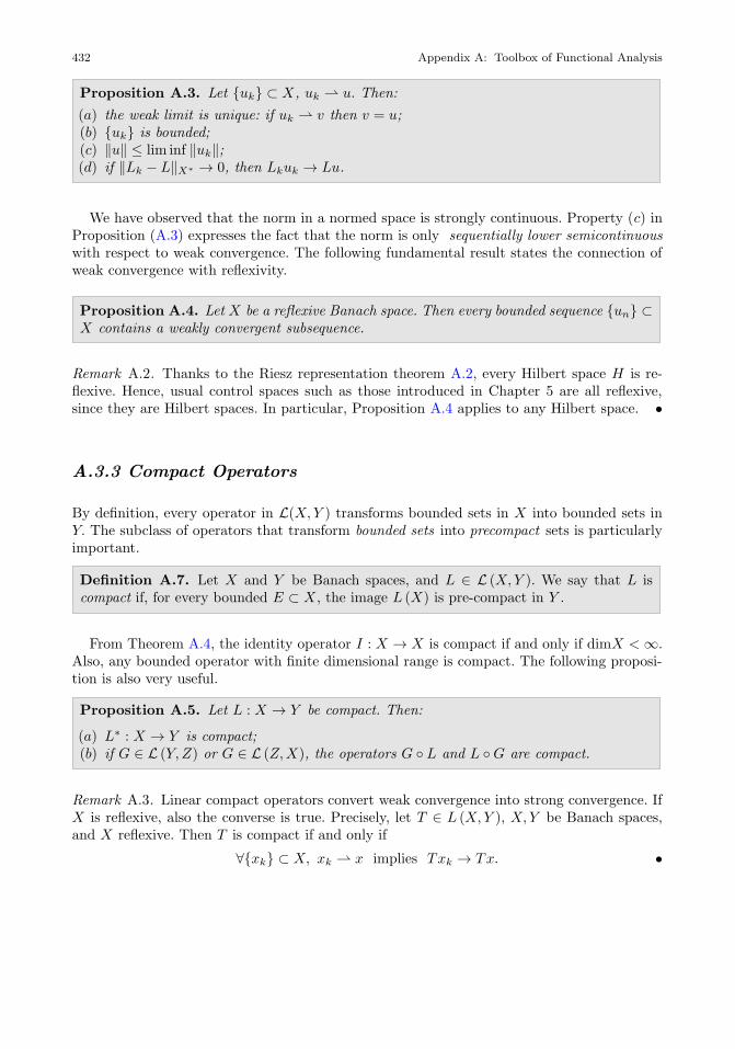
Proposition A.3. Let uk ⊂ X, uk u. Then:
(a) the weak limit is unique: if uk v then v = u;(b) uk is bounded;(c) ‖u‖ ≤ lim inf ‖uk‖;(d) if ‖Lk − L‖X∗ → 0, then Lkuk → Lu.
We have observed that the norm in a normed space is strongly continuous. Property (c) inProposition (A.3) expresses the fact that the norm is only sequentially lower semicontinuouswith respect to weak convergence. The following fundamental result states the connection ofweak convergence with reflexivity.
Proposition A.4. Let X be a reflexive Banach space. Then every bounded sequence un ⊂X contains a weakly convergent subsequence.
Remark A.2. Thanks to the Riesz representation theorem A.2, every Hilbert space H is re-flexive. Hence, usual control spaces such as those introduced in Chapter 5 are all reflexive,since they are Hilbert spaces. In particular, Proposition A.4 applies to any Hilbert space. •
A.3.3 Compact Operators
By definition, every operator in L(X,Y ) transforms bounded sets in X into bounded sets inY. The subclass of operators that transform bounded sets into precompact sets is particularlyimportant.
Definition A.7. Let X and Y be Banach spaces, and L ∈ L (X,Y ). We say that L iscompact if, for every bounded E ⊂ X, the image L (X) is pre-compact in Y .
From Theorem A.4, the identity operator I : X → X is compact if and only if dimX <∞.Also, any bounded operator with finite dimensional range is compact. The following proposi-tion is also very useful.
Proposition A.5. Let L : X → Y be compact. Then:
(a) L∗ : X → Y is compact;(b) if G ∈ L (Y,Z) or G ∈ L (Z,X), the operators G L and L G are compact.
Remark A.3. Linear compact operators convert weak convergence into strong convergence. IfX is reflexive, also the converse is true. Precisely, let T ∈ L (X,Y ), X,Y be Banach spaces,and X reflexive. Then T is compact if and only if
∀xk ⊂ X, xk x implies Txk → Tx. •
A.3 Compactness and Weak Convergence 433
A.3.4 Convexity and Weak Closure
We have seen in Sect. A.3.2 that a strongly convergent sequence is also weakly convergent:however, not always a property holding in the strong sense also holds in the weak one. Forinstance, a (strongly) closed set in a Banach space X is not necessarily weakly sequentiallyclosed. The sequence xk of Example A.6 is contained in the unit sphere S1 of L2 (0, 2π),which is a closed set in this space. However xk 0 /∈ S1, and therefore S1 is not weaklysequentially closed.
Here convexity comes into play: as soon as the (strongly) closed set is also convex, it is alsoweakly sequentially closed, according to the following
Proposition A.6. Let K ⊆ X be a closed convex set. Then K is weakly sequentially closed.
Thus, a convex set is closed if and only if it is weakly sequentially closed.
A.3.5 Weak∗ Convergence, Separability and Weak∗ SequentialCompactness
In several problems the natural space where we seek a control variable is not reflexive. This isfor instance the case in which a control u ≥ 0 acts as a reaction coefficient or a potential in astate equation like
−∆y + uy = f in Ω,
or as a diffusion coefficient in
−div (u∇y) = f in Ω.
In these situations u ∈ L∞(Ω), which is not a reflexive Banach space, see Sect. A.5.1.When reflexivity is lacking, weak convergence is not appropriate to recover compactness. In
fact, the dual X∗ of a Banach space can be endowed with another type of convergence, calledweak∗ convergence.
Definition A.8. We say that a sequence Lk ⊂ X∗ converges weakly∗ to L ∈ X∗, and
we write Lk∗ L, if
Lku→ Lu ∀u ∈ X. (A.14)
Remark A.4. If X is reflexive, the weak∗ convergence is nothing else than weak convergencein X∗. •
For the weak∗ convergence an analog of Proposition A.4 holds.
Proposition A.7. Let X be a Banach space and Lk ⊂ X∗ such that Lk∗ L. Then:
(a) the weak∗ limit is unique: if Lk∗ G then G = L;
(b) Lk is bounded in X∗;(c) if ‖uk − u‖X → 0, then Lkuk → Lu.
434 Appendix A: Toolbox of Functional Analysis
The relevance of weak∗ convergence relies in the following fundamental result that states aconnection with the separability of X. We recall that X is separable if there exists a countablesubset D which is dense in X, that is D ⊆ X and D = X.
Theorem A.5 (Banach-Alaoglu). If X is separable, any bounded sequence in X∗ containsa weakly∗ convergent subsequence.
A.4 Abstract Variational Problems
We recall in this section some results essential for the correct variational formulation of abroad variety of boundary value problems, including several examples of state problems foroptimal control problems discussed along this book.
In particular, we briefly review (strongly) coercive and saddle-point problems, presentingthe main well-posedness results; see, e.g., [224, 64, 121, 237, 218, 41] for their proofs.
In this context, a key role is played by bilinear forms. Given two linear spaces V,W , abilinear form in V ×W is a map
a : V ×W → Rsatisfying the following properties:
(i) for every y ∈W , the function x 7→ a(x, y) is linear in V ;(ii) for every x ∈ V , the function y 7→ a(x, y) is linear in W .
When V = W , we simply say that a is a bilinear form in V .
A.4.1 Coercive Problems
Let V be a Hilbert space, a be a bilinear form in V and F ∈ V ∗ (the dual space of V ). Considernow the following problem, called abstract variational problem:
find y ∈ V such thata (y, v) = 〈F, v〉V ∗,V ∀v ∈ V. (P1)
The fundamental result is provided by the following
Theorem A.6 (Lax-Milgram). Let V be a real Hilbert space endowed with inner product(·, ·) and norm ‖·‖, and a(·, ·) a bilinear form in V which is:
(i) continuous, i.e. there exists a constant M such that
|a(v, w)| ≤M ‖v‖ ‖w‖ ∀v, w ∈ V ;
(ii) V−coercive, i.e. there exists a constant α > 0 such that
a(v, v) ≥ α ‖v‖2 ∀v ∈ V. (A.15)
Then, problem (P1) has a unique solution y ∈ V . Moreover, y satisfies the stability estimate
‖y‖ ≤ 1
α‖F‖V ∗ . (A.16)
A.4 Abstract Variational Problems 435
If a is also symmetric, then it induces in V the inner product
(v, w)a = a (v, w) .
In this case, existence, uniqueness and stability for problem (P1) follow directly from RieszRepresentation Theorem A.2. Moreover (see Sect. 5.1.2), by defining the quadratic functional
J(v) =1
2a(v, v)− 〈F, v〉V ∗,V , (A.17)
the following property holds.
Proposition A.8. Let V be a real Hilbert space, a : V × V → R a continuous, symmetricand positive bilinear form on V × V , and F ∈ V ∗. Then, u is the (unique) solution of (P1)if and only if
J(u) = minv∈V
J(v). (A.18)
A.4.2 Saddle-Point Problems
Mixed variational problems or saddle point problems do not fall in the class of coercive prob-lems, thus requiring a different treatment1. Two remarkable cases, addressed in this book,are Stokes equations and the optimality system arising from unconstrained linear-quadraticOCPs. For a more in-depth reading we refer e.g. to [41].
Given two Hilbert spaces X and Q along with their duals X∗ and Q∗, respectively, thebilinear forms e : X×X → R, b : X×Q→ R and F1 ∈ X∗, F2 ∈ Q∗, we consider the followingmixed variational problem:
find (x, p) ∈ X ×Q such thate(x,w) + b(w, p) = 〈F1, w〉W∗,W ∀w ∈ Xb(x, q) = 〈F2, q〉Q∗,Q ∀q ∈ Q.
(P2)
The following theorem [53, 41] establishes sufficient conditions for the saddle-point problem(P2) to be well posed. Let us denote by
X0 = w ∈ X : b(w, q) = 0 ∀q ∈ Q ⊂ X.
Theorem A.7. Assume that the following conditions hold:
1. e(·, ·) is continuous, i.e. there exists Me > 0 such that
|e(x,w)| ≤Me‖x‖X‖w‖X ∀x,w ∈ X; (A.19)
2. e(·, ·) is weakly coercive on X0, i.e. there exists α0 > 0 such that
infx∈X0
supw∈X0
e(x,w)
‖x‖X‖w‖X≥ α0, inf
w∈X0
supx∈X0
e(x,w) > 0; (A.20)
1 These are special instances of weakly coercive problems, which can be analyzed according to the Necas
Theorem, see, e.g., [203] for further details. This may happen if, for instance, (i) in (P1) a(·, ·) fails to becoercive, or (ii) y ∈ V but we ask the variational equation to hold for every ϕ ∈W 6= V , with F ∈W ∗.
436 Appendix A: Toolbox of Functional Analysis
3. b(·, ·) is continuous, i.e. there exists Mb > 0 such that
|b(w, q)| ≤Mb‖w‖X‖q‖Q ∀w ∈ X, q ∈ Q; (A.21)
4. the bilinear form b(·, ·) satisfies the inf-sup condition, i.e. there exists βs0 > 0 such that
infq∈Q
supw∈X
b(w, q)
‖w‖X‖q‖Q≥ βs0. (A.22)
Then, there exists a unique solution (x, p) ∈ X ×Q to the mixed variational problem (P2).Moreover, the following stability estimates hold:
‖x‖X ≤1
α
[‖f1‖X∗ +
α0 +Me
βs0‖F2‖Q∗
], (A.23a)
‖p‖Q ≤1
βs0
[(1 +
Me
α0
)‖F1‖X∗ +
Me(α0 +Me)
α0 + βs0‖F2‖Q∗
]. (A.23b)
Remark A.5. Note that if e(·, ·) is symmetric, the second condition in (A.20) automaticallyfollows from the first one. •
We have seen that for symmetric bilinear forms the variational problem (P1) is equivalentto a minimization problem for the quadratic functional J defined in (A.17). Similarly, thefollowing result states that the mixed variational problem (P2) is equivalent to a constrainedminimization problem for the same quadratic functional, provided e(·, ·) is a symmetric andpositive bilinear form, in the following sense.
Given a linear mapping L : X ×Q→ R, (x, p) is called a saddle point of L if
L(x, q) ≤ L(x, p) ≤ L(w, p) ∀(w, q) ∈ X ×Q,or equivalently,
infw∈X
supq∈QL(w, q) = sup
q∈QL(x, q) = L(x, p) = inf
w∈XL(w, p) = sup
q∈Qinfw∈X
L(w, q).
Proposition A.9. Let X and Q be two Hilbert spaces and consider the functionals F1 ∈ X∗and F2 ∈ Q∗, as well as the bilinear forms e(·, ·) and b(·, ·) on X×X and X×Q, respectively.Assume that d : X ×X → R is symmetric and positive. Then (x, p) ∈ X ×Q is a solutionto problem (P2) if and only if (x, p) is a saddle point of
L(w, q) =1
2e(w,w) + b(w, q)− 〈F1, w〉X∗,X − 〈F2, q〉Q∗,Q , (A.24)
that is, if and only if x is a minimizer of
J(w) =1
2e(w,w)− 〈F1, w〉X∗,X
over X under the constraint b(x, q) = 〈F2, q〉Q∗,Q ∀q ∈ Q. Equivalently,
x = arg minw∈X
J(w) subject to b(x, q) = 〈F2, q〉Q∗,Q ∀q ∈ Q. (A.25)
If, additionally, the assumptions of Theorem A.7 are fulfilled, problem (P2) has a uniquesolution, which is the unique saddle point of L.
Hence, (P2) can be seen as a set of first-order necessary (and sufficient) optimality conditionsfor the constrained minimization problem (A.25).

A.5 Sobolev spaces 437
A.5 Sobolev spaces
Sobolev spaces provide the natural functional setting for the PDEs that we consider in thistextbook. After introducing their definition, we recall the main results concerning these spaces.It is understood that by a measure |E| of a set E ⊆ Rd we mean the Lebesgue measure definedover the (σ−algebra of the) Lebesgue measurable sets. Accordingly, if Ω is a measurable set,a function u : Ω → R, is measurable if the set x ∈ Ω : u (x) > t is measurable ∀t ∈ R. Fora survey on measure theory we refer, e.g., to [234, 280].
A.5.1 Lebesgue Spaces
Let Ω be an open set in Rd and p ∈ R, p ≥ 1. We denote by Lp (Ω) the set of measurablefunctions u : Ω → R such that |u|p is Lebesgue integrable2 in Ω. Identifying two functions uand v when they are equal a.e.3 in Ω, Lp (Ω) becomes a Banach space when equipped withthe norm (integral norm of order p)
‖u‖Lp(Ω) =
(∫
Ω
|u|p)1/p
.
L2 (Ω) is a Hilbert space when endowed with the inner product
(u, v)L2(Ω) =
∫
Ω
uv.
The identification of two functions equal a.e. amounts to saying that an element of Lp (Ω) isnot a single function but, actually, an equivalence class of functions, different from one anotheronly on subsets of zero measure. When dealing with a function in Lp (Ω), for most practicalpurposes, one may refer to the more convenient representative of the class. However, as weshall see later, some care is due, especially when pointwise properties are involved.
The symbol L∞ (Ω) denotes the set of essentially bounded functions in Ω. We say thatu : Ω → R is essentially bounded if there exists M such that
|u (x)| ≤M a.e. in Ω. (A.26)
The infimum of all numbers M with the property (A.26) is called essential supremum of u,and denoted by
‖u‖L∞(Ω) = ess supΩ|u| .
Note that the essential supremum may differ from the supremum. As an example, take thecharacteristic function of the rational numbers
χQ(x) =
1 x ∈ Q,0 x ∈ R \Q. (A.27)
Then supR χQ = 1, but ‖χQ‖L∞(Ω) = 0, since Q has zero Lebesgue measure.
If we identify two functions when they are equal a.e., ‖u‖L∞(Ω) is a norm in L∞ (Ω), and
L∞ (Ω) becomes a Banach space.
2 A basic introduction on the construction of the Lebesgue integral can be found, e.g., in [237].3 A property is valid almost everywhere in a set Ω, a.e. in short, if it is true at all points in Ω, but for asubset of measure zero.
438 Appendix A: Toolbox of Functional Analysis
We list below some relevant results concerning the Lp spaces.
Lemma A.1 (Holder inequality). Let p ∈ [1,∞] and q = p/(p − 1) be its dual exponent(with q = 1,∞ if p =∞, 1, respectively). If u ∈ Lp (Ω), v ∈ Lq (Ω), then
∫
Ω
|uv| ≤ ‖u‖Lp(Ω) ‖v‖Lq(Ω) . (A.28)
A more general version of the Holder inequality, involving three functions, states that ifp, q, r ∈ [1,∞] with 1/p+ 1/q + 1/r = 1, and u ∈ Lp(Ω), v ∈ Lq(Ω), and w ∈ Lr(Ω), then
∫
Ω
|uvw| ≤ ‖u‖Lp(Ω) ‖v‖Lq(Ω) ‖w‖Lr(Ω) . (A.29)
Note that, if Ω has finite measure and 1 ≤ p1 < p2 ≤ ∞, from (A.28) we have, choosing v = 1and taking |u|p1 as u , p = p2/p1 and q = p2/(p2 − p1),
∫
Ω
|u|p1 ≤ |Ω|1/q ‖u‖p1Lp2 (Ω)
where |Ω| denotes the Lebesgue measure of Ω, then Lp2 (Ω) ⊂ Lp1 (Ω). If the measure of Ωis infinite, this inclusion is not true, in general; for instance, f = 1 belongs to L∞ (R) but notto Lp (R) for 1 ≤ p <∞.
Lemma A.2. For every p ∈ [1,∞], the dual of Lp (Ω) is identified with Lq (Ω), whereq = p/ (p− 1).
This means that for p ∈ (1,∞) the space Lp(Ω) is reflexive. The spaces Lp (Ω), 1 ≤ p <∞are all separable; L∞ (Ω) is not.
Remark A.6. If X∗ is separable, so is X, but clearly the converse is false. For instance, L∞ (Ω)is the dual of L1 (Ω). •
Let C∞ (Ω) be the set of infinitely differentiable functions in Ω and C∞0 (Ω) be the set ofall functions u ∈ C∞ (Ω) vanishing outside a compact subset of Ω. Then:
Lemma A.3. C∞0 (Ω) is dense in Lp (Ω) for any 1 ≤ p <∞.
As a consequence, we have the following useful result, where L1loc (Ω) denotes the set of
functions integrable on every compact subset of Ω.
Lemma A.4. If u ∈ L1loc (Ω) and
∫
Ω
uϕ = 0 for all ϕ ∈ C∞0 (Ω) ,
then u = 0 almost everywhere.
The following result is a cornerstone of the Lebesgue theory.
A.5 Sobolev spaces 439
Theorem A.8 (Lebesgue dominated convergence). Let uk : Ω → R, k ≥ 1, be a sequenceof measurable functions such that:
(i) uk → u a.e. in Ω;(ii) there exists g ∈ L1 (Ω) such that |uk| ≤ g a.e. in Ω ∀k ≥ 1.
Then uk, u ∈ L1 (Ω) and ‖uk − u‖L1(Ω) → 0 as k →∞.
A.5.2 Domain Regularity
A domain Ω ⊂ Rd can be classified according to the degree of smoothness of its boundaryΓ = ∂Ω (see Fig. A.1).
Definition A.9. We say that Ω ⊂ Rd is a C1−domain if for every point p ∈ Γ there existsa system of coordinates (y1, . . . , yd−1, yd) = (y′, yd) with origin at p, a ball B (p) and afunction ϕ defined in a neighborhood Np ⊂ Rd−1 of y′ = 0′ such that
ϕ ∈ C1 (Np) , ϕ (0′) = 0
andΓ ∩B (p) = (y′, yd) : yd = ϕ (y′) , y′ ∈ Np ,Ω ∩B (p) = (y′, yd) : yd > ϕ (y′) , y′ ∈ Np .
In other words, Γ locally coincides with the graph of a C1−function, and Ω is locally placedon one side of its boundary.
The boundary of a C1−domain does not have corners or edges and for every point p ∈ Γ ,a tangent straight line (d = 2) or plane (d = 3) or hyperplane (d > 3) is well defined,together with the outward normal unit vectors n = (n1, . . . , nd). Moreover these vectors varycontinuously on Γ . The couples (ϕ,Np) appearing in the above definition are called localcharts. If the functions ϕ are all Ck−functions, for some k ≥ 1, Ω is said to be a Ck−domain;if this is true for every k ≥ 1, Ω is a C∞−domain (or smooth domain).
In several applications the relevant domains are rectangles, prisms, cones, cylinders orunions of them; moreover, polygonal domains obtained by triangulation procedures of smoothdomains are very often employed in numerical approximation, see Sect. B.4. All these areLipschitz domains, described by local charts where all the functions ϕ are Lipschitz continuous.
Fig. A.1 A C1 domain (left) and a Lipschitz domain (right)
440 Appendix A: Toolbox of Functional Analysis
A.5.3 Integration by Parts and Weak Derivatives
The following integration by parts formula holds: let Ω be a bounded, Lipschitz domain inRd; if u, v ∈ C1
(Ω), then∫
Ω
uxjv dx =
∫
Γ
uv njdσ −∫
Ω
uvxjdx, j = 1, . . . , d (A.30)
where dσ denotes the surface area element; in terms of local charts, dσ =
√1 + |∇ϕ|2dy′.
The notion of derivative in a weak sense (weak derivative or distributional derivative) relieson the fact that, using formula (A.30), for functions u ∈ C1
(Ω)
the following relation holds∫
Ω
uxjϕ dx =−∫
Ω
uϕxjdx ∀ϕ ∈ C∞0 (Ω) . (A.31)
Observing that the right hand side in (A.31) makes sense for u ∈ L1loc (Ω), we are led to the
following definition.
Definition A.10. Let Ω ⊆ Rd be open and u ∈ L1loc (Ω). A function w ∈ L1
loc (Ω) is calledthe weak partial xj−derivative of u, if
∫
Ω
wϕ dx =−∫
Ω
uϕxjdx ∀ϕ ∈ C∞0 (Ω) , j = 1, . . . , d. (A.32)
We use the same symbols uxj , ∂xju or ∂u/∂xj to denote the weak xj−derivative of u.Note that w is uniquely determined thanks to Lemma A.4. Similarly, for any multi-indexα = (α1, . . . , αd), |α| > 0, the α− th weak partial derivative of u, w = Dαu is defined by therelation ∫
Ω
wϕ dx = (−1)|α|∫
Ω
uDαϕdx ∀ϕ ∈ C∞0 (Ω) . (A.33)
A.5.4 The Space H1 (Ω)
Let Ω ⊆ Rd be an open set. The Sobolev space H1 (Ω) is the subspace of L2 (Ω) of thefunctions u having weak first partial derivatives which belong to L2 (Ω). Precisely:
Definition A.11. The Sobolev space H1 (Ω) is defined by
H1(Ω) =u ∈ L2(Ω) : u has weak derivatives uxj ∈ L2 (Ω) , j = 1, . . . , d
.
The weak gradient ∇u is a vector whose components are the weak first partial derivativesof u; then u ∈ H1(Ω) if ∇u ∈ L2(Ω)d. Since in several contexts the Dirichlet integral
∫
Ω
|∇u|2
represents an energy, the functions in H1 (Ω) are associated with configurations having finiteenergy.
A.5 Sobolev spaces 441
Proposition A.10. Endowed with the inner product
(u, v)H1(Ω) =
∫
Ω
uv dx +
∫
Ω
∇u · ∇v dx
H1(Ω) is a Hilbert space, continuously embedded in L2(Ω).
Example A.7. Let Ω = B1/2 (0) =x ∈ R2 : |x| < 1/2
and u (x) = (− log |x|)a, x 6= 0. Using
polar coordinates, we find
∫
B1/2(0)
u2dx = 2π
∫ 1/2
0
(− log r)2ardr <∞ ∀a ∈ R,
so that u ∈ L2(B1/2 (0)
)for every a ∈ R. Moreover,
uxi = −axi |x|−2(− log |x|)a−1
, i = 1, 2
and therefore |∇u| = |a (− log |x|)a−1 | |x|−1. Still using polar coordinates,
∫
B1/2(0)
|∇u|2 dx = 2πa2
∫ 1/2
0
|log r|2a−2r−1dr.
This integral is finite only if 2 − 2a > 1 or a < 1/2. In particular, ∇u represents the gradientof u in the weak sense. We conclude that u ∈ H1 (B1 (0)) only if a < 1/2. We point out thatwhen a > 0, u is unbounded near 0. •
As Example A.7 shows, a function in H1 (Ω) may be unbounded. In dimension d = 1 thiscannot occur. In fact, the elements in H1 (a, b) are continuous functions4 in [a, b].
Proposition A.11. Let u ∈ L2 (a, b). Then u ∈ H1 (a, b) if and only if u is continuous in[a, b] and there exists w ∈ L2 (a, b) such that
u(y) = u(x) +
∫ y
x
w (s) ds ∀x, y ∈ [a, b]. (A.34)
Moreover u′ = w (both a.e. and in the weak sense).
Remark A.7. Since a function u ∈ H1 (a, b) is continuous in [a, b], the value u (x0) at everypoint x0 ∈ [a, b] makes sense. •
A.5.5 The Space H10 (Ω) and its Dual
We introduce an important subspace of H1 (Ω).
Definition A.12. We denote by H10 (Ω) the closure of C∞0 (Ω) in H1 (Ω).
Hence, u ∈ H10 (Ω) if and only if there exists a sequence ϕk ⊂ C∞0 (Ω) such that ϕk → u
in H1 (Ω), that is, ‖ϕk − u‖L2(Ω) → 0 and ‖∇ϕk −∇u‖L2(Ω) → 0 as k → ∞. Since the
test functions in C∞0 (Ω) vanish on Γ , every u ∈ H10 (Ω) “inherits” this property and it is
4 Rigorously: every equivalence class in H1 (a, b) has a representative continuous in [a, b].
442 Appendix A: Toolbox of Functional Analysis
reasonable to consider H10 (Ω) as the set of functions in H1 (Ω) vanishing on Γ . Clearly,
H10 (Ω) is a Hilbert subspace of H1 (Ω).In the applications of the Lax-Milgram theorem to boundary value problems, the dual of
H10 (Ω) plays an important role and it is denoted by H−1(Ω).
Theorem A.9. F ∈ H−1(Ω) if and only if there exists f0 ∈ L2(Ω) and f = (f1, . . . , fd) ∈L2(Ω)d such that
〈F, v〉H−1,H10
= (f0, v)L2(Ω) + (f ,∇v)L2(Ω) ; (A.35)
moreover,
‖F‖H−1(Ω) ≤‖f0‖L2(Ω) + ‖f‖L2(Ω)
. (A.36)
Hence, the elements of H−1(Ω) are represented by a linear combination of functions inL2(Ω) and their weak first derivatives. In particular, L2(Ω) → H−1(Ω).
An important property of H10 (Ω), particularly useful in the analysis of boundary value
problems, is the Poincare inequality5.
Theorem A.10. Let Ω ⊂ Rd be a bounded domain. Then, there exists a positive constantCP = CP (d, diam (Ω)) (Poincare constant) such that
‖u‖L2(Ω) ≤ CP ‖∇u‖L2(Ω)d ∀u ∈ H10 (Ω) . (A.37)
Inequality (A.37) implies that, if Ω is bounded, the norm ‖u‖H1(Ω) is equivalent to
‖∇u‖L2(Ω)d in H10 (Ω). Indeed
‖u‖H1(Ω) =√‖u‖2L2(Ω) + ‖∇u‖2L2(Ω)d
and from (A.37)‖∇u‖L2(Ω)d ≤ ‖u‖H1(Ω) ≤
√C2P + 1 ‖∇u‖L2(Ω)d .
In the space H1(Ω), ‖∇u‖L2(Ω)d only defines a seminorm, denoted by
|u|H1(Ω) = ‖∇u‖L2(Ω)d .
Example A.8 (Weak convergence). We characterize the weak convergence in L2(Ω) andH10 (Ω).
We have that uk ⊂ L2 (Ω) converges weakly to u if∫
Ω
ukϕ→∫
Ω
uϕ ∀ϕ ∈ L2 (Ω) .
Similarly, uk ⊂ H10 (Ω) converges weakly to u if
∫
Ω
∇uk · ∇ϕ→∫
Ω
∇u · ∇ϕ ∀ϕ ∈ H10 (Ω) . •
Remark A.8. The optimal constant CP in the Poincare inequality is usually referred to asthe Poincare constant for the domain Ω. Its determination is related with the solution of aneigenvalue problem for the Laplace operator. Indeed, denoting by
λ1 = minu∈H1
0 (Ω),u 6=0R(u), R(u) =
∫Ω|∇u|2dx∫Ωu2dx
,
5 Recall that the diameter of a set Ω is given by diam (Ω) = supx,y∈Ω |x− y|.
A.5 Sobolev spaces 443
we have that
‖u‖L2(Ω) ≤1√λ1
‖∇u‖L2(Ω)d
and equality holds when u is an eigenvector corresponding to λ1. R(u) is usually called theRayleigh quotient. Hence, 1/
√λ1 is the best (i.e. the smallest) Poincare constant for the
domain Ω. See, e.g., [237, Chapter 8] for further details and related proofs. •Another very useful result (see e.g. [276] for the proof) is provided by the following Garding
inequality, helpful when dealing with weakly coercive problems.
Proposition A.12. Let a : V × V → R be a bilinear form in V , H10 (Ω) ⊂ V ⊂ H1(Ω),
such that:
1. it fulfills the Garding inequality: for some constants α > 0 and λ > 0
a(v, v) ≥ α‖v‖2V − λ‖v‖2L2(Ω) ∀v ∈ V ; (A.38)
2. if u ∈ V is such that a(u, v) = 0 for any v ∈ V , then u = 0.
Then there exists a constant β = β(λ) > 0 such that
supw∈V
a(v, w)
‖w‖V≥ β‖v‖V ∀v ∈ V.
Indeed, a bilinear form fulfilling inequality (A.38) is often called weakly coercive.
A.5.6 The Spaces Hm (Ω), m > 1
Involving higher order derivatives, we may construct new Sobolev spaces. Let N be the numberof multi-indexes α = (α1, . . . , αd), αj ≥ 0, such that |α| = ∑d
i=1 αi ≤ m. We denote by Hm(Ω)the Sobolev space of the functions in L2 (Ω), whose weak derivatives up to order m included,are functions in L2 (Ω), that is (with slight abuse of notation)
Hm(Ω) =u ∈ L2(Ω) : Dαu ∈ L2(Ω) ∀α : |α| ≤ m
.
Proposition A.13. Equipped with the inner product
(u, v)Hm(Ω) =∑
|α|≤m
∫
Ω
DαuDαv dx
Hm(Ω) is a Hilbert space, continuously embedded in L2(Ω). Moreover,
‖u‖Hm(Ω) =
(‖u‖2L2(Ω) +
m∑
k=1
|u|2Hk(Ω)
)1/2
. (A.39)
where |u|Hk(Ω) denotes the following seminorm in Hk(Ω), k = 1, . . . ,m,
|u|Hk(Ω) =
√∑
|α|=k
‖Dαu‖2L2(Ω).
If u ∈ Hm (Ω), any derivative of u of order k belongs to Hm−k (Ω); more generally, if|α| = k ≤ m, then Dαu ∈ Hm−k (Ω) and Hm(Ω) → Hm−k (Ω), k ≥ 1.
444 Appendix A: Toolbox of Functional Analysis
Example A.9. Let B1/2 (0) ⊂ R3 and consider u (x) = |x|−a; then, u ∈ H1(B1/2 (0)
)if
a < 1/2. The second order derivatives of u are given by
uxixj = a (a+ 2)xixj |x|−a−4 − aδij |x|−a−2.
Then |uxixj | ≤ |a (a+ 2) | |x|−a−2so that uxixj ∈ L2
(B1/2 (0)
)if 2a+ 4 < 3, or a < − 1
2 . Thus
u ∈ H2(B1/2 (0)
)if a < −1/2. •
We denote by Hm0 (Ω) the closure of C∞0 (Ω) with respect to the norm (A.39). The elements
in Hm0 (Ω) “vanish” on Γ together with all their derivatives of order up to m− 1 included.
More in general, for k ≥ 0 integer, and 1 ≤ p ≤ ∞, we define the Sobolev spaces
W 1,p (Ω) =u ∈ Lp (Ω) : ∇u ∈ Lp (Ω)
d.
A.5.7 Approximation by Smooth Functions. Traces
A function u ∈ H1 (Ω) is, in principle, defined only up to a set of zero measure. However,if Ω is a bounded Lipschitz domain, it is possible to approximate any element in H1 (Ω) bysmooth functions in C∞
(Ω), the set of infinitely differentiable functions, whose derivatives of
any order can be continuously extended up to Γ . In other terms,
C∞(Ω)
=∞⋂
k=1
Ck(Ω).
Proposition A.14. Let Ω be a bounded Lipschitz domain. Then C∞(Ω)
is dense inH1 (Ω) .
The possibility of approximating any element u ∈ H1 (Ω) by smooth functions in Ω rep-resents a key tool for introducing the notion of restriction of u on Γ , denoted by u|Γ . Suchrestriction is called the trace of u on Γ and it will be an element of L2 (Γ ). Since Γ is a setof zero measure, this notion is subtle and has to be addressed in a rather indirect way, byintroducing a suitable trace operator, as shown in the following theorem.
Theorem A.11. Let Ω ⊂ Rd be a bounded, Lipschitz domain. Then there exists a linearoperator (trace operator) τ0 : H1(Ω)→ L2 (Γ ) such that
τ0u = u|Γ if u ∈ C∞(Ω)
and‖τ0u‖L2(Γ ) ≤ ctr ‖u‖H1(Ω) (trace inequality), (A.40)
for a suitable constant ctr = ctr (Ω, d); τ0u is called the trace of u on Γ .
It is not surprising that the kernel of τ0 is precisely H10 (Ω), that is,
τ0u = 0 if and only if u ∈ H10 (Ω) .
For the trace τ0u we also use the notation u|Γ and, if there is no risk of confusion, inside aboundary integral we will simply write
∫Γu dσ.
A.5 Sobolev spaces 445
The operator τ0 : H1 (Ω) → L2 (Γ ) is not surjective. In fact, the image of τ0 is strictlycontained in L2 (Γ ) . In other words, there are functions in L2 (Γ ) which are not traces offunctions in H1(Ω). We use the symbol H1/2 (Γ ) to denote Imτ0, that is,
H1/2 (Γ ) =τ0u : u ∈ H1(Ω)
. (A.41)
H1/2 (Γ ) is a Hilbert space with norm given by
‖g‖H1/2(Γ ) = inf‖w‖H1(Ω) : w ∈ H1(Ω), τ0w = g
. (A.42)
This norm is equal to the smallest among the norms of all elements in H1(Ω) sharing thesame trace g on Γ and takes into account that the trace operator τ0 is not injective, since weknow that Ker τ0 = H1
0 (Ω).In particular, the following trace inequality holds
‖τ0u‖H1/2(Γ ) ≤ ‖u‖H1(Ω) , (A.43)
which means that the trace operator τ0 is continuous from H1(Ω) onto H1/2 (Γ ) .We denote by H−1/2 (Γ ) the dual space of H1/2 (Γ ).
Remark A.9. It is possible to define a semi-norm in H1/2(Γ ) thanks to the so-called Steklov-Poincare operator. Indeed, for any g ∈ H1/2(Γ ), there exists a unique function ug ∈ H1(Ω),called the harmonic extension of g, fulfilling
−∆ug = 0 in Ω
ug = g on Γ.(A.44)
Exploiting the Green’s identity, we can formally define the following semi-norm
|g|2H1/2(Γ ) =
∫
Γ
∂ug∂n
ugdσ =
∫
Ω
|∇ug|2dx. (A.45)
By introducing the Steklov-Poincare operator S : H1/2(Γ )→ H−1/2(Γ ),
Sg =∂ug∂n
(A.46)
realizing the so-called Dirichlet-to-Neumann map [225] related to problem (A.44), we canrewrite (A.45) rigorously as
|g|2H1/2(Γ ) = 〈Sg, g〉H−1/2,H1/2 .
As a consequence,‖g‖2H1/2(Γ ) = ‖g‖2L2(Γ ) + |g|2H1/2(Γ ).
See, e.g., [209] for further details about applications in the field of OCPs. •In a similar way, we may define the trace of u ∈ H1 (Ω) on a smooth subset Γ0 ⊂ Γ .
Theorem A.12. Assume that Ω ⊂ Rd is a bounded, Lipschitz domain. Let Γ0 be a smoothsubset of Γ. Then there exists a trace operator τΓ0
: H1(Ω)→ L2 (Γ0) such that
τΓ0u = u|Γ0
if u ∈ C∞(Ω),
and‖τΓ0
u‖L2(Γ0) ≤ ctr (Ω, d) ‖u‖H1(Ω) (trace inequality). (A.47)

446 Appendix A: Toolbox of Functional Analysis
The function τΓ0u is called the trace of u on Γ0, often denoted by u|Γ0
. For the kernel ofτΓ0, a Hilbert subspace of H1 (Ω), we use the symbol H1
Γ0(Ω), that is
τΓ0u = 0 if and only if u ∈ H1
Γ0(Ω) .
This space can be characterized in another way. Let VΓ0 be the set of functions in C∞(Ω)
vanishing in a neighborhood of Γ 0. Then H1Γ0
(Ω) is the closure of VΓ0under the norm in
H1 (Ω).
Proposition A.15. The Poincare inequality holds in H1Γ0
(Ω). Therefore, ‖∇u‖L2(Ω)d is
a norm in H1Γ0
(Ω).
We use the symbol H1/2 (Γ0) to denote the image of τΓ0, that is,
H1/2 (Γ0) =τΓ0
u : u ∈ H1(Ω). (A.48)
H1/2 (Γ0) is a Hilbert space with induced norm given by
‖g‖H1/2(Γ0) = inf‖w‖H1(Ω) : w ∈ H1(Ω), τΓ0
w = g.
In particular,‖τΓ0u‖H1/2(Γ0) ≤ ‖u‖H1(Ω) (A.49)
which means that the trace operator τΓ0 is continuous from H1(Ω) onto H1/2 (Γ0).
A.5.8 Compactness
Since‖u‖L2(Ω) ≤ ‖u‖H1(Ω) ,
H1 (Ω) is continuously embedded in L2 (Ω) that is, if a sequence uk converges to u in H1 (Ω)it converges to u in L2 (Ω) as well.
If we assume that Ω is a bounded, Lipschitz domain, then the embedding of H1 (Ω) inL2 (Ω) is also compact. Thus, for any bounded sequence uk ⊂ H1 (Ω), there exists a subse-quence
ukj
and u ∈ H1 (Ω) such that
ukj → u in L2 (Ω) and ukj u in H1 (Ω) .
Actually, only the former property follows from the compactness of the embedding; thelatter – i.e., the fact that ukj converges weakly to u in H1 (Ω) – expresses indeed a generalfact in every Hilbert space H, since every bounded subset E ⊂ H is sequentially weaklycompact (see Proposition A.4). We can state the following
Theorem A.13 (Rellich). Let Ω be a bounded, Lipschitz domain. Then H1 (Ω) is com-pactly embedded in L2 (Ω). Moreover, under the same assumptions, H1/2 (Γ ) is dense andcompactly embedded in L2 (Γ ).
A.5 Sobolev spaces 447
A.5.9 The space Hdiv(Ω)
Another space which is indeed useful when dealing with incompressible fluid flows is Hdiv(Ω).
Definition A.13. Let Ω ⊂ Rd, d ≥ 2, be a bounded Lipschitz domain. Then
Hdiv(Ω) = u ∈ L2(Ω)d : divu ∈ L2(Ω)is a Sobolev space, with norm
‖u‖Hdiv(Ω) =(‖u‖2L2(Ω) + ‖divu‖2L2(Ω)
)1/2
and inner product
(u,v)Hdiv(Ω) =
∫
Ω
u · v dx +
∫
Ω
divu divv dx.
Hdiv(Ω) is a separable Hilbert space, continuously embedded into L2(Ω)d. For each u ∈H1(Ω)d ⊂ Hdiv(Ω), d ≥ 2, we can define the trace of each component ui on Γ = ∂Ω and,consequently, the so-called normal trace of u,
u · n =d∑
i=1
ui|Γni.
Since C∞(Ω)d is dense also in Hdiv(Ω), the normal trace can be defined for vectors of Hdiv(Ω),according to the following
Theorem A.14. Assume Ω ⊂ Rd is a bounded, Lipschitz domain. Then there exists alinear operator (normal trace operator) τ : Hdiv(Ω)→ H−1/2(Γ ) such that
τu = u · n|Γ if u ∈ C∞(Ω)d
and‖τu‖H−1/2(Γ ) ≤ c(Ω, d)‖u‖Hdiv(Ω).
Moreover, for each u ∈ Hdiv(Ω) and each ϕ ∈ H1(Ω), the following generalized integrationby parts formula holds
∫
Ω
∇ϕ · u dx = −∫
Ω
ϕdivu dx + 〈u · n, ϕ〉H−1/2,H1/2 . (A.50)
A.5.10 The Space H1/200 and Its Dual
The treatment of mixed problems for Stokes and Navier-Stokes equations requires the intro-duction of other trace spaces. In general, if Γ0 is a smooth subset of Γ and u ∈ H1/2(Γ0), thetrivial extension u of u to Γ , that is u = u on Γ0 and u = 0 on Γ1 = Γ\Γ 0, does not belong6
to H1/2 (Γ ). Thus, we introduce the new space
H1/200 (Γ0) =
u ∈ H1/2 (Γ0) : u ∈ H1/2 (Γ )
.
6 Take for instance Ω = (−2, 2)2 ⊂ R2 and Γ0 = (−1, 1) × 0. The characteristic function of Γ0 does not
belong to H1/2 (Γ ) (although it is not trivial to prove it) while clearly the function v = 1 on Γ0 belongs toH1/2 (Γ0) since it is the trace of the function identically equal to 1 on Ω.
448 Appendix A: Toolbox of Functional Analysis
In other terms, H1/200 (Γ0) is the space of traces on Γ0 of elements in H
1/2Γ1
(Ω). H1/200 (Γ0) is
a Hilbert space if endowed with the norm ‖u‖H
1/200 (Γ0)
= ‖u‖H1/2(Γ ). We denote its dual by
H−1/200 (Γ0) and the duality between H
−1/200 (Γ0) and H
1/200 (Γ0) by the symbol 〈·, ·〉Γ0
.It turns out that
H1/200 (Γ0) ⊂ L2 (Γ0) ⊂ H−1/2
00 (Γ0)
is a Hilbert triplet, with H1/200 (Γ0) compactly embedded into L2 (Γ0). In particular, if u ∈
L2 (Γ0), v ∈ H1/200 (Γ0) then
〈u, v〉Γ0= (u, v)L2(Γ0) .
Using these spaces, it is possible to define the normal trace u · n of u ∈ Hdiv (Ω)d
on Γ0.Indeed, we can define u · n|Γ0
as the restriction to Γ0 of the trace u · n|Γ ∈ H−1/2 (Γ ). Thisrestriction requires some care.
In fact, let F ∈ H−1/2 (Γ ). If F and v were functions in L2 (Γ0), the action of F|Γ0on v
would be defined by
F|Γ0v =
∫
Γ
F v.
The functional F|Γ0acts on the trivial extension of v. Therefore, the restriction to Γ0 of
F ∈ H−1/2 (Γ ) must act on H1/200 (Γ0) and be an element of H
−1/200 (Γ0). Its action is defined
by the formula⟨F|Γ0
, v⟩Γ0
= 〈F, v〉H−1/2(Γ ),H1/2(Γ ) ∀v ∈ H1/200 (Γ0) . (A.51)
Going back to the normal trace of u ∈ Hdiv (Ω)d
on Γ0, we conclude that u · n|Γ0is well
defined as an element in H−1/200 (Γ0). Moreover, the following integration by parts formula
holds ∫
Ω
∇v · u dx = −∫
Ω
v divu dx +⟨u · n|Γ0
, v⟩Γ0
∀v ∈ H1Γ1
(Ω) .
A.5.11 Sobolev Embeddings
We know that the elements of H1 (a, b) are actually continuous functions in [a, b]. In dimensiond ≥ 2, the functions in H1 (Ω) enjoy a better summability property, as indicated in thefollowing theorem.
Theorem A.15. Let Ω ⊂ Rd be a bounded, Lipschitz domain. Then:
1. If d > 2, H1(Ω) → Lp (Ω) for 2 ≤ p ≤ 2dd−2 .
Moreover, if 2 ≤ p < 2dd−2 , the embedding of H1(Ω) in Lp (Ω) is compact;
2. if d = 2, H1(Ω) → Lp (Ω) for 2 ≤ p <∞, with compact embedding.
In the above cases‖u‖Lp(Ω) ≤ c(d, p,Ω) ‖u‖H1(Ω) .
For instance, if d = 3, 2dd−2 = 6, hence
H1(Ω) → L6 (Ω) and ‖u‖L6(Ω) ≤ c(Ω) ‖u‖H1(Ω) .
Theorem A.15 shows that H1-functions can enjoy better summability properties than justL2(Ω). For Hm-functions, with m > 1, the following regularity theorem holds.
A.6 Functions with Values in Hilbert Spaces 449
Theorem A.16. Let Ω be a bounded, Lipschitz domain, and m > d/2. Then
Hm(Ω) → Ck,α(Ω), (A.52)
for k integer, 0 ≤ k < m− d2 and α = 1/2 if d is odd, α ∈ (0, 1) if d is even. The embedding
in (A.52) is compact and
‖u‖Ck,α(Ω) ≤ c(d,m, α,Ω) ‖u‖Hm(Ω) .
Theorem A.16 implies that, in dimension d = 2, two derivatives occur to get (Holder)continuity
H2(Ω) → C0,α(Ω), 0 < α < 1.
In fact, in this case d is even, m = 2, and m− d2 = 1. Similarly
H3(Ω) → C1,a(Ω), 0 < α < 1,
since m− d2 = 2.
In dimension d = 3 we have
H2(Ω) ⊂ C0,1/2(Ω)
and H3(Ω) ⊂ C1,1/2(Ω),
since m− d2 = 1
2 in the former case and m− d2 = 3
2 in the latter.
Remark A.10. If u ∈ Hm(Ω) for any m ≥ 1, then u ∈ C∞(Ω). This kind of results is very
useful in the regularity theory of boundary value problems. •
A.6 Functions with Values in Hilbert Spaces
Let V be a separable Hilbert space (e.g. L2 (Ω) orH1 (Ω)). We consider functions y : [0, T ]→ Vand introduce the main functional spaces we are going to use.
A.6.1 Spaces of Continuous Functions
We start by introducing the set C ([0, T ];V ) of the continuous functions y : [0, T ] → V ,endowed with the norm
‖y‖C([0,T ];V ) = max0≤t≤T
‖y (t)‖V .
Clearly C ([0, T ];V ) is a Banach space. We say that v : [0, T ]→ V is the (strong) derivative vof y if ∥∥∥∥
y (t+ h)− y (t)
h− v (t)
∥∥∥∥V
→ 0
for each t ∈ [0, T ]. We write as usual y′ or y for the derivative of y.The symbol C1 ([0, T ];V ) denotes the Banach space of functions whose derivative exists
and belongs to C ([0, T ];V ) , endowed with the norm
‖y‖C1([0,T ];V ) = ‖y‖C([0,T ];V ) + ‖y′‖C([0,T ];V )
Similarly we can define the spaces Ck ([0, T ] ;V ) and C∞ ([0, T ] ;V ) , while C∞0 (0, T ;V ) de-notes the subspace of C∞ ([0, T ] ;V ) of the functions compactly supported in (0, T ).
450 Appendix A: Toolbox of Functional Analysis
A.6.2 Integrals and Spaces of Integrable Functions
The notions of measurability and integral (called Bochner integral) can be extended to thesetypes of functions. First, we introduce the set of functions s : [0, T ] → V which assume onlya finite number of values; they are called simple and take the form
s (t) =N∑
j=1
χEj (t) yj , 0 ≤ t ≤ T, (A.53)
where y1, . . . , yN ∈ V and E1, . . . , EN are Lebesgue measurable, mutually disjoint subsets of[0, T ]. We say that f : [0, T ] → V is measurable if there exists a sequence of simple functionssk : [0, T ]→ V such that, as k →∞,
‖sk (t)− f (t)‖V → 0 a.e. in [0, T ] .
It is not difficult to prove that, if f is measurable and v ∈ V , the (real) function t 7−→(f (t) , v)V is Lebesgue measurable in [0, T ].
The notion of integral is defined first for simple functions. If s is given by (A.53), we define
∫ T
0
s (t) dt =N∑
j=1
|Ej | yj
with the convention that |Ej | yj = 0 if yj = 0. We thus provide the following
Definition A.14. We say that f : [0, T ]→ V is summable in [0, T ] if it is measurable andthere exists a sequence sk : [0, T ]→ V of simple functions such that
∫ T
0
‖sk (t)− f (t)‖V dt→ 0 as k → +∞. (A.54)
If f is summable in [0, T ], we define the integral of f as follows
∫ T
0
f (t) dt = limk→+∞
∫ T
0
sk (t) dt as k → +∞. (A.55)
The limit (A.55) is well defined and does not depend on the choice of the approximatingsequence sk. Moreover, the following important theorem holds.
Theorem A.17 (Bochner). A measurable function f : [0, T ]→ V is summable in [0, T ] ifand only if the real function t 7−→ ‖f (t)‖V is summable in [0, T ]. Moreover
∥∥∥∥∥
∫ T
0
f (t) dt
∥∥∥∥∥V
≤∫ T
0
‖f (t)‖V dt (A.56)
and (u,
∫ T
0
f (t) dt
)
V
=
∫ T
0
(u, f (t))V dt, ∀u ∈ V. (A.57)
The inequality (A.56) is well known in the case of real or complex functions. Thanks to theRiesz Representation Theorem, (A.57) shows that the action of any element of V ∗ commuteswith the integrals.
A.6 Functions with Values in Hilbert Spaces 451
Once the definition of integral has been given, we can introduce the space Lp (0, T ;V ),1 ≤ p ≤ ∞, as the set of measurable functions y : [0, T ]→ V such that:
• if 1 ≤ p <∞,
‖y‖Lp(0,T ;V ) =
(∫ T
0
‖y (t)‖pV dt)1/p
<∞; (A.58)
• if p =∞‖y‖L∞(0,T ;V ) = ess sup
0≤t≤T‖y (t)‖V <∞.
Endowed with the above norms, Lp (0, T ;V ) becomes a Banach space for 1 ≤ p ≤ ∞. If p = 2,the norm (A.58) is induced by the inner product
(y, v)L2(0,T ;V ) =
∫ T
0
(y (t) , v (t))V dt
that makes L2 (0, T ;V ) a Hilbert space.
If y ∈ L1 (0, T ;V ), the function t 7−→∫ t
0y (s) ds is continuous and
d
dt
∫ t
0
y (s) ds = y (t) a.e. in (0, T ) .
Proposition A.16. C∞0 (0, T ;V ) is dense in Lp (0, T ;V ) , 1 ≤ p <∞.
A.6.3 Sobolev Spaces Involving Time
To define Sobolev spaces, we need the notion of derivative in the sense of distributions forfunctions y ∈ L1
loc (0, T ;V ). We say that y′ ∈ L1loc (0, T ;V ) is the derivative in the sense of
distributions of y if ∫ T
0
ϕ (t) y′ (t) dt = −∫ T
0
ϕ′ (t) y (t) dt (A.59)
for every ϕ ∈ C∞0 (0, T ) or, equivalently, if∫ T
0
ϕ (t) (y′ (t) , v)V dt = −∫ T
0
ϕ′ (t) (y (t) , v)V dt ∀v ∈ V . (A.60)
We denote by H1 (0, T ;V ) the Sobolev space of the functions y ∈ L2 (0, T ;V ) such thaty′ ∈ L2 (0, T ;V ). This is a Hilbert space with inner product
(y, ϕ)H1(0,T ;V ) =
∫ T
0
(y (t) , ϕ (t))V + (y′ (t) , ϕ′ (t))V dt.
Since functions in H1 (a, b) are continuous in [a, b], it makes sense to consider the value ofy at any point of [a, b]. In a certain way, the functions in H1 (0, T ;V ) depend only on the realvariable t, so that the following theorem is not surprising.
452 Appendix A: Toolbox of Functional Analysis
Theorem A.18. Let u ∈ H1 (0, T ;V ). Then, u ∈ C ([0, T ];V ) and
max0≤t≤T
‖u (t)‖V ≤ C (T ) ‖u‖H1(0,T ;V ) .
Moreover, the fundamental theorem of Calculus holds,
u (t) = u (s) +
∫ t
s
u′ (r) dr, 0 ≤ s ≤ t ≤ T.
If V and W are separable Hilbert spaces with V → W , it makes sense to define the Sobolevspace
H1 (0, T ;V,W ) =y ∈ L2 (0, T ;V ) : y′ ∈ L2 (0, T ;W )
,
where y′ is intended in the sense of distributions in C∞0 (0, T ;W ), endowed with the scalarproduct
(y, ϕ)H1(0,T ;V,W ) =
∫ T
0
(y (t) , ϕ (t))V + (y′ (t) , ϕ′ (t))W dt.
and the norm‖y‖H1(0,T ;V,W ) =
(‖y‖2L2(0,T ;V ) + ‖y′‖2L2(0,T ;W )
)1/2
.
This situation typically occurs in the applications to initial-boundary value problems. Givena Hilbert triplet (see Sect. A.2.3) V → H → V ∗, with V and H separable, the naturalfunctional setting is precisely the space H1 (0, T ;V, V ∗). The following result (whose proofcan be found, e.g., in [73, Volume 5, Chapter XVIII]) is of fundamental importance.
Theorem A.19. Let (V,H, V ∗) be a Hilbert triplet, with V and H separable. Then:
(a) C∞ ([0, T ] ;V ) is dense in H1 (0, T ;V, V ∗);(b) H1 (0, T ;V, V ∗) → C ([0, T ] ;H), that is
‖u‖C([0,T ];H) ≤ C (T ) ‖u‖H1(0,T ;V,V ∗) ;
(c) (Aubin Lemma) H1(0, T ;V, V ∗) is compactly embedded into L2(0, T ;H);(d) if y, ϕ ∈ H1 (0, T ;V, V ∗), the following integration by parts formula holds,
∫ t
s
〈y′ (r) , ϕ (r)〉∗ + 〈y (r) , ϕ′ (r)〉∗ dr = (y (t) , ϕ (t))H − (y (s) , ϕ (s))H (A.61)
for all s, t ∈ [0, T ].
From (A.61) we infer that
d
dt(y (t) , ϕ (t))H = 〈y′ (t) , ϕ (t)〉∗ + 〈y (t) , ϕ′ (t)〉∗
a.e. t ∈ [0, T ] and (letting ϕ = y)∫ t
s
d
dt‖y (r)‖2H dt = ‖y (t)‖2H − ‖y (s)‖2H . (A.62)
A.7 Differential Calculus in Banach Spaces 453
A.6.4 The Gronwall Lemma
When dealing with initial-boundary value problems, the following result proves to be extremelyuseful in order to derive stability estimates (see, e.g., [224, Chap. 1] for the proof).
Lemma A.5 (Gronwall). Let A ∈ L1(0, T ) be a non-negative function, ϕ a continuousfunction on [0, T ]. If g is non-decreasing and ϕ is such that
ϕ(t) ≤ g(t) +
∫ t
0
A(τ)ϕ(τ)dτ ∀t ∈ [0, T ],
then
ϕ(t) ≤ g(t) exp
(∫ t
t0
A(τ)dτ
)∀t ∈ [t0, T ].
A.7 Differential Calculus in Banach Spaces
In order to write first order optimality conditions for OCPs in Banach spaces, we need somecalculus in infinite dimensional vector spaces.
A.7.1 The Frechet Derivative
We start by generalizing the notion of differential to operators between Banach spaces.
Definition A.15. Let X and Y be Banach spaces, and U ⊆ X be a (non-empty) open sub-set of X. An operator F : U → Y is called Frechet differentiable (briefly F−differentiable)at x0 ∈ U if there exists an operator L (x0) ∈ L (X,Y ) such that if h ∈ U and x0 + h ∈ U ,
F (x0 + h)− F (x0) = L (x0)h+R (h, x0) (A.63)
with R (h, x0) = o (‖h‖X), that is
limh→0
‖R (h, x0)‖Y‖h‖X
= 0. (A.64)
L (x0) is called Frechet derivative (or differential) of F at x0, and we write L (x0) = F ′ (x0).
The following properties hold:
a) Uniqueness. The Frechet derivative F ′ (x0) is unique; indeed, if L1, L2 ∈ L (X,Y ) andboth satisfy (A.63), then we would have (L1 − L2)h = o (‖h‖X), which implies L1 = L2.
b) F−differentiability =⇒ continuity. If F is F−differentiable at x0 then it is continuous atx0; in fact, letting h→ 0 in (A.63) we get F (x0 + h)− F (x0)→ 0.
c) Linearity. Frechet differentiation is a linear operation: if F,G : U ⊆ X → Y areF−differentiable at x0, and r, s ∈ R, then rF + sG is F−differentiable at x0 with
(rF + sG)′(x0) = rF ′(x0) + sG′(x0).
454 Appendix A: Toolbox of Functional Analysis
d) Different norms. Let X → X and the operator F : X → Y be F−differentiable atx0 ∈ X. Then F is differentiable at x0 when regarded as an operator from X to Y and theanalytical expression of the derivative does not change7. In particular, if F is differentiablewith respect to a given norm, then it is also differentiable with respect to a stronger norm.If we introduce two equivalent norms over X or Y , a differentiable function with respectto one norm is still differentiable with respect to the other norm and its derivative doesnot change.
e) Chain rule. The chain rule for the derivation of the composition of functions still holds.Let X,Y, Z be Banach spaces, F : U ⊆ X → V ⊆ Y and G : V ⊆ Y → Z, where Uand Vare open sets. If F is F -differentiable at x0 and G is F -differentiable at y0 = F (x0), thenG F is F -differentiable at x0 and
(G F )′ (x0) = G′ (y0) F ′ (x0) .
Example A.10. If F is constant, then F ′ = 0. If F ∈ L (X,Y ), F is differentiable at any pointand F ′ (x) = F for every x ∈ X. •Example A.11. Let X,Y, Z be Banach spaces. Introduce over X × Y the norm
‖(x, y)‖X×Y = (‖x‖2 + ‖y‖2)1/2
and let F : X × Y → Z be a bilinear and continuous operator, that is x 7→ F (x, y) andy 7→ F (x, y) are linear for y and x respectively fixed, and there exists a number C such that
‖F (x, y)‖Z ≤ C ‖x‖X ‖y‖Y ∀ (x, y) ∈ X × Y.Then F is differentiable and F ′ (x0, y0) is the linear map
(h, k) 7−→ F (x0, k) + F (h, y0) .
In fact,F (x0 + h, y0 + k)− F (x0, y0)
= F (x0 + h, y0 + k)− F (x0 + h, y0) + F (x0 + h, y0)− F (x0, y0)= F (x0 + h, k) + F (h, y0) = F (x0, k) + F (h, y0) + F (h, k) .
Moreover, F (h, k) = o (‖ (h, k) ‖X×Y ); indeed,
‖F (h, k)‖Z‖ (h, k) ‖X×Y
≤ C ‖h‖X ‖k‖Y(‖h‖2 + ‖k‖2)1/2
≤ C
2‖ (h, k) ‖X×Y ,
which tends to 0 as ‖ (h, k) ‖X×Y → 0. •
If F is F−differentiable at every point of U , the map
F ′ : U → L (X,Y )
given by x 7−→ F ′ (x) is called the Frechet derivative of F . We say that F is continuouslyF−differentiable and we write F ∈ C1 (U ;Y ) , if F ′ is continuous in U , that is if for anyx, x0 ∈ U we have
‖F ′ (x)− F ′ (x0)‖L(X,Y ) → 0 if ‖x− x0‖X → 0.
7 Note that X → X means that ‖x‖X ≤ c ‖x‖X ∀x ∈ X, for a given constant c > 0. If L ∈ L (X,Y ), then
‖x‖Y ≤ ‖L‖L(X,Y ) ‖x‖X ≤ c ‖L‖L(X,Y ) ‖x‖X ∀x ∈ X and hence L ∈ L(X,Y ) implies L ∈ L(X, Y ). Then, it is
possible to show that (A.63) holds with the same L, regarded as element of L(X, Y ), and R (h, x0) = o(‖h‖X
).
A.7 Differential Calculus in Banach Spaces 455
In the special case Y = R, we have L (X,R) = X∗ and therefore if J : U ⊆ X → R isF−differentiable at any point of U , its Frechet derivative is a map J ′ : U → X∗. Thus, theaction of J ′ (x) on an element h of X is given by the duality
J ′ (x)h = 〈J ′ (x) , h〉X∗,X ,
and we can simply write 〈J ′ (x) , h〉∗ if there is no risk of confusion.If moreover X is a Hilbert space with inner product (·.·), through the Riesz canonical
isomorphism R (see Theorem A.2) we can identify X∗ with X. The application RJ ′ deservesa special name and leads to the following definition.
Definition A.16. Let H be a Hilbert space and J : U ⊆ H → R be F−differentiable atany point of U . The application
R J ′ : U ⊆ H → H
is called the gradient of J and is denoted by∇J . Equivalently,∇J is defined by the followingrelation 〈J ′ (u) , v〉∗ = (∇J (u) , v) ∀u ∈ U, ∀v ∈ H. (A.65)
Example A.12. Quadratic functionals over a Hilbert space. Let H be a Hilbert space withinner product (·, ·) and norm ‖·‖. Let a : H ×H → R be a bilinear, symmetric and continuousform on H (see Sect. A.4) and J : H → R be the quadratic functional
J (u) =1
2a (u, u) .
We want to show that J ∈ C1 (H) = C1 (H;R) , that
〈J ′ (u) , v〉∗ = a (u, v) ∀u, v ∈ H (A.66)
and to compute ∇J . Since a is bilinear and symmetric, we have
J (u+ v)− J (u) =1
2a (u+ v, u+ v)− 1
2a (u, u)
= a (u, v) +1
2a (v, v) = a (u, v) + o (‖v‖)
as a (v, v) ≤M ‖v‖2 . We can conclude that J is F -differentiable and (A.66) holds. Moreover,
〈J ′ (u+ h)− J ′ (u) , v〉∗ = a (h, v)
and then, since a is continuous,
‖J ′ (u+ h)− J ′ (u)‖H∗ = sup‖v‖=1
|〈J ′ (u+ h)− J ′ (u) , v〉∗| ≤M ‖h‖
from which we deduce the (Lipschitz) continuity of J ′.Now we compute ∇J . From Riesz Representation Theorem A.2, there exists an element
ua = R J ′ (u) such that we can rewrite (A.66) under the form
〈J ′ (u) , v〉∗ = (ua, v) ∀u, v ∈ H.
Therefore∇J (u) = ua.
456 Appendix A: Toolbox of Functional Analysis
In particular, let z0 ∈ H and consider the functional
J (u) =1
2‖u− z0‖2 =
1
2‖u‖2 − (z0, u) +
1
2‖z0‖2 .
Then J ∈ C1 (H) and〈J ′ (u0) , v〉∗ = (u0 − z0, v) ,
so that∇J (u0) = u0 − z0. •
The Frechet partial derivatives of an operator F : U ⊆ X × Y → Z,
F ′x ∈ L (X,Z) , F ′y ∈ L (Y, Z)
at a point (x0, y0) ∈ U , can be defined by the following relations: for every h ∈ X, k ∈ Y ,
F (x0 + h, y0)− F (x0, y0) = F ′x (x0, y0)h+ o (‖h‖X) ,
F (x0, y0 + k)− F (x0, y0) = F ′y (x0, y0) k + o (‖k‖X) .
As in the finite dimensional case, the following result holds:
Proposition A.17. If F ′x : U → L (X,Z) and F ′y : U → L (Y,Z) are continuous at(x0, y0) ∈ U , then F is F -differentiable at (x0, y0) and
F ′(x0, y0) (h, k) = F ′x(x0, y0)h+ F ′y(x0, y0)k ∀h ∈ X, ∀k ∈ Y.
A.7.2 The Gateaux Derivative
A weaker notion of derivative is that of Gateaux derivative, which generalizes the concept ofdirectional derivative.
Definition A.17. Let X and Y be Banach spaces, and U ⊆ X be an open subset of X.An operator F : U ⊆ X → Y is called Gateaux differentiable (briefly G−differentable) atx0 ∈ U if there exists an operator A (x0) ∈ L (X,Y ), such that, for any h ∈ X and anyt ∈ R such that x0 + th ∈ U ,
limt→0
F (x0 + th)− F (x0)
t= A (x0)h.
A (x0) is called the Gateaux derivative (or differential) of F at x0 and we write A (x0) =F ′G (x0).
If F is G−differentiable at any point in U , the application F ′G : U → L (X,Y ) given by
F ′G : x 7→ F ′G (x)
is called Gateaux derivative of F . The following properties hold:
a) uniqueness. The Gateaux derivative at x0 is unique;
b) commutativity with linear bounded functionals. The Gateaux differentiation commutes withany linear and continuous functional. In fact, if y∗ ∈ Y ∗ and F is G−differentiable in a
A.7 Differential Calculus in Banach Spaces 457
neighborhood of x0, we can write
d
dt〈y∗, F (x0 + th)〉 = lim
s→0
⟨y∗,
F (x0 + th+ sh)− F (x0 + th)
s
⟩
=⟨y∗, F ′G(x0 + th)h
⟩
and, in particular,d
dt〈y∗, F (x0 + th)〉|t=0 =
⟨y∗, F ′G(x0)h
⟩;
c) chain rule. The chain rule holds in the following form: if F is G−differentiable at x0 andG is F -differentiable at y0 = F (x0), then G F is G-differentiable at x0 and
(G F )′G (x0) = G′ (y0) F ′G (x0) ; (A.67)
d) F and G−differentiability. If F is F -differentiable at x0, then it is also G-differentiable atx0 and F ′ (x0) = F ′G (x0). Conversely, we have:
Proposition A.18. Let F : U ⊆ X → Y be G−differentiable in U. If F ′G is continuous atx0, then F is F-differentiable at x0 and F ′ (x0) = F ′G (x0).
This latter result is often employed to show the F−differentiability of a given operator; infact it is often simpler to compute the Gateaux derivative and show that it is a continuousoperator, than to check directly the F -differentiability.
A.7.3 Derivative of Convex Functionals
When dealing with minimization problems, convex functionals play a relevant role. As alreadyseen in the finite dimensional case, uniqueness of the minimizer is guaranteed for strictlyconvex functionals.
Let J : U ⊆ X → R be a G−differentiable functional in U . Then, J ′G (x) ∈ X∗ for anyx ∈ U , that is, J ′G : U → X∗. To denote the action of J ′G (x) (or of any other element of X∗)over h ∈ X, we will use the symbols
J ′G (x)h or⟨J ′G (x) , h
⟩∗ or
⟨J ′G (x) , h
⟩X∗,X
depending on the context. The following result (strictly related to OCPs, hence providedtogether with its proof) holds:
Theorem A.20. Let U be an open convex set and J : U ⊆ X → R be a G−differentiablefunctional on U . The following properties are equivalent:
1. J is convex;2. for any x, y ∈ U
J (y) ≥ J (x) +⟨J ′G (x) , y − x
⟩∗ ; (A.68)
3. J ′G is a monotone operator in the following sense
⟨J ′G (x)− J ′G (y) , x− y
⟩∗ ≥ 0 ∀x, y ∈ U. (A.69)
458 Appendix A: Toolbox of Functional Analysis
Proof. (1)⇒ (2). Fix x, y ∈ U . Since J is convex, for all t ∈ (0, 1) we have
J (x+ t(y − x))− J (x) ≤ t (J (y)− J (x)) .
Dividing by t and letting t→ 0+ we get⟨J ′G (x) , (y − x)
⟩∗ ≤ J (y)− J (x) . (A.70)
(2)⇒ (3). Exchanging the roles of x and y in (A.70), we obtain⟨J ′G (y) , (x− y)
⟩∗ ≤ J (x)− J (y) . (A.71)
By summing up (A.70) and (A.71) we deduce (A.69).
(3)⇒ (1). Set g (t) = J (x+ t(y − x)), t ∈ [0, 1] and compute
g′ (t) =⟨J ′G (x+ t (y − x)) , (y − x)
⟩∗
Thus, if t > s,
g′ (t)− g′ (s) =⟨J ′G (x+ t (y − x))− J ′G (x+ s (y − x)) , (y − x)
⟩∗
=1
t− s⟨J ′G (x+ t (y − x))− J ′G (x+ s (y − x)) , (t− s) (y − x)
⟩∗ ≥ 0.
It follows that g′ is nondecreasing, therefore g is convex and hence, for t ∈ (0, 1),
g (t) ≤ g (0) + t[g (1)− g (0)]
which is the convexity of J . ut
We point out that when in (A.68) and (A.69) the inequality is replaced by a strict inequalityfor any x, y ∈ U, x 6= y, both these conditions are equivalent to the strict convexity of J .
Example A.13. We return to the case of quadratic functionals discussed in Sect. A.7.1. If thebilinear form a is nonnegative, that is a (v, v) ≥ 0 ∀v ∈ U , then the functional
J (u) =1
2a (u, u)
is convex. In fact, since 〈J ′ (u) , v〉∗ = a (u, v), we have that
J (u+ v)− J (u) = a (u, v) +1
2a (v, v) ≥ a (u, v) ∀v ∈ U .
If a is positive, that is, a (v, v) > 0 ∀v ∈ U , v 6= 0, J is clearly strictly convex. •
Example A.14. Let Ω ⊂ Rd be a bounded Lipschitz domain. The operator Φ : L6 (Ω)→ L2 (Ω)given by
Φ : y 7→ y3
is F−differentiable at every point and
Φ′ (y)h = 3y2h ∀y, h ∈ L6(Ω).
This follows by a straightforward application of the definition (A.15). By property d) inSect. A.7.2, Φ is also F−differentiable as an operator from H1 (Ω) into L2 (Ω), provided d ≤ 3.Moreover Φ′ : L6 (Ω) → L
(L6 (Ω) , L2 (Ω)
)is continuous. In fact, using Holder inequality
(A.29) with exponents p = q = r = 1/3,
‖[Φ′ (y + z)− Φ′ (y)]h‖L2(Ω) =∥∥3(y2 − z2
)h∥∥L2(Ω)
≤ 3 ‖y + z‖L6(Ω) ‖y − z‖L6(Ω) ‖h‖L6(Ω)
whence
A.7 Differential Calculus in Banach Spaces 459
‖Φ′ (y + z)− Φ′ (y)‖L(L6(Ω),L2(Ω)) = sup‖h‖L6(Ω)=1
‖[Φ′ (y + z)− Φ′ (y)]h‖L2(Ω)
≤ 3 ‖y + z‖L6(Ω) ‖y − z‖L6(Ω)
and Φ′ is (locally Lipschitz) continuous. •Example A.15. Let Φ : Lp (0, 1)→ Lp (0, 1) be given by
Φ : y → sin y.
Then Φ is G−differentiable for every p, 1 ≤ p ≤ ∞, with
Φ′G (y)h = cos (y)h ∀y, h ∈ Lp(Ω).
In fact, we can show that
sin (y (x) + th (x))− sin (y (x))
t− cos (y (x))h (x) = R (t; y, h)
with
R (t; y, h) = −h (x)
∫ 1
0
[cos(y (x) + sth (x))− cos (y (x))] ds.
Since R (t; y, h)→ 0 as t→ 0 and |R (t; y, h)| ≤ 2 |h| ∈ Lp (0, 1), by the Lebesgue’s dominatedconvergence Theorem A.8 we conclude that ‖R (t; y, h)‖Lp(0,1) → 0 as t → 0 and therefore is
G−differentiable with Φ′G (y)h = cos (y)h. •Remark A.11. In general, if 1 ≤ p < ∞, Φ : y 7→ sin y is not F−differentiable, at any point.Indeed, it can be proved that an operator Φ : Lp (Ω)→ Lp (Ω) given by
Φ : y 7→ F (y)
is F−differentiable if and only if F (y) = cy for some constant c. •
Remark A.12. Maps of the form Φ : y → f (x,y) are known as Nemytskii operators (see, e.g.[231, Section 10.3.4]). •
Example A.16. Let F ∈ C2 (R). The operator Φ : L∞ (Ω)→ L∞ (Ω) given by
Φ : y → F (y)
is F−differentiable withΦ′ (y)h = F ′ (y)h, (A.72)
and that Φ′ : L∞ (Ω)→ L (L∞ (Ω) , L∞ (Ω)) is (locally Lipschitz) continuous.Indeed, we can write, for a.e. x ∈ Ω,
F (y(x) + h(x))− F (y (x))
=
∫ 1
0
d
dtF (y (x) + th (x))dt =
∫ 1
0
F ′(y (x) + th (x))h (x) dt
= F ′(y (x))h (x) + h (x)
∫ 1
0
[F ′(y (x) + th (x))− F ′ (y (x))] dt
= F ′(y (x))h (x) + E (y (x) , h (x))
and
460 Appendix A: Toolbox of Functional Analysis
F ′(y (x) + th (x))− F ′ (y (x)) =
∫ t
0
d
dsF ′(y (x) + sh (x))ds
=
∫ t
0
F ′′ (y (x) + sh (x))h (x) ds.
Then,‖E (y, h)‖L∞(Ω) ≤ ‖h‖
2L∞(Ω) ‖F ′′ (y (x) + sth (x))‖L∞(Ω) ≤ C ‖h‖
2L∞(Ω)
where C = sups∈[0,1],x∈Ω
|F ′′ (y (x) + sh (x))|. Thus, we can deduce that Φ is F -differentiable and
that (A.72) holds. With the same method, it is possible to show that Φ′ is (locally Lipschitz)continuous. •
A.7.4 Second Order Derivatives∗
As in Definition A.15, let F : U ⊆ X → Y be a F− differentiable operator, where U is anopen subset of X. The mapping y 7→ F ′ (y) defines an operator from U into L (X,Y ).
Definition A.18. The operator F : U ⊆ X → Y is twice differentiable at y ∈ U if theoperator u 7→ F ′ (y) is F−differentiable at y ∈ U . (F ′)′ is called the second derivative of Fand we can write F ′′ (y) = (F ′)
′(y); moreover, we have
F ′′ (y) ∈ L (X,L (X,Y )) .
Thus, F ′′ (y) is a bounded linear operator from X into L (X,Y ).
More explicitly, given h ∈ X, F ′′ (y)h represents a bounded linear operator in L (X,Y ),whose action on another element k ∈ X is given by (F ′′ (y)h)k ∈ Y . Therefore, F ′′ (y) can beidentified (see, e.g., [57, Sect. 5.1]) with a continuous bilinear form from X ×X into Y , andits action can be denoted by
(h, k) 7→ F ′′ (y) [h, k] ; (A.73)
in particular, we setF ′′ (y) [h2] = F ′′ (y) [h, h].
With these notations, we have that
‖F ′′ (y)‖L(X,L(X,Y )) = sup‖h‖=1,‖k‖=1
‖F ′′ (y) [h, k]‖Y .
A result by Cartan (see [57, Thm. 5.1.1]) asserts that the continuous bilinear form (A.73) issymmetric, that is
(F ′′ (y)h)k = (F ′′ (y) k)h or F ′′ (y) [h, k] = F ′′ (y) [k, h] .
In the particular case Y = R, we have F ′′ (y) ∈ L (X,X∗), so that F ′′ (y)h ∈ X∗ and, for itsaction on k ∈ X, we may use the (hybrid) notation
〈F ′′ (y)h, k〉X∗,X .
For twice F−differentiable operators, the following Taylor expansion holds:
A.7 Differential Calculus in Banach Spaces 461
F (y + h) = F (y) + F ′ (y)h+1
2F ′′ (y) [h2] + ε (y, h) ‖h‖2X (A.74)
with‖ε (y, h)‖Y → 0 as ‖h‖X → 0.
If F is twice differentiable at every point y ∈ U , the mapping y 7→ F ′′ (y) from U intoL (X,L (X,Y )) is well defined. If this mapping is continuous, that is if
‖F ′′ (y)− F ′′ (y0)‖L(X,L(X,Y )) → 0 as ‖y − y0‖X → 0,
we say that F ′′ is twice continuously F− differentiable.
Example A.17. We go back to Example A.14, and consider Φ : L6 (Ω)→ L2 (Ω) : y 7→ y3. Wehave seen that
Φ′ (y) : L6 (Ω)→ L(L6 (Ω) , L2 (Ω))
is given by the multiplication operator
h 7→ 3y2h
We now show that Φ′ is continuously F−differentiable, with
Φ′′ (y) : L6 (Ω)→ L(L6 (Ω) ,L(L6 (Ω) , L2 (Ω))
given byΦ′′ (y) [h, k] = 6yhk.
Indeed,Φ′ (y + h)− Φ′ (y)− 6yh = 3h2,
to be intended as a multiplication operator from L6 (Ω) into L2 (Ω). By the three-factorsHolder inequality (A.29), with p = q = r = 3,
∥∥h2∥∥L(L6(Ω),L2(Ω))
= sup‖k‖L6(Ω)=1
∥∥h2k∥∥L2(Ω)
≤ ‖h‖2L6(Ω) ;
hence, ‖Φ′ (y + h)− Φ′ (y)− 6yh‖L2(Ω)
‖h‖L6(Ω)
→ 0 as ‖h‖L6(Ω) → 0.
The (Lipschitz) continuity of Φ′′ follows by the following relationship,
‖Φ′′ (y)− Φ′′ (z)‖L(L6(Ω),L(L6(Ω),L2(Ω)) = 6 sup‖h‖L6(Ω)=‖k‖L6(Ω)=1
‖(y − z)hk‖L2(Ω)
≤ 6 ‖y − z‖L6(Ω) .
•Example A.18. The operator Φ : L∞ (Ω)→ L∞ (Ω) given by
u 7→ f (u)
already considered in Example A.16 is twice continuously F−differentiable, with
Φ′′ (u) : L∞ (Ω)→ L(L∞ (Ω) , L∞ (Ω)∗)
given byΦ′′ (u) [h, k] = f ′′ (u)hk.
•Example A.19. The functional F : L∞ (Ω)→ R given by
462 Appendix A: Toolbox of Functional Analysis
F (y) =1
6
∫
Ω
y6dx
is twice continuously F−differentiable, with
F ′ (y)h =
∫
Ω
y5h dx (A.75)
and
F ′′ (y) [h, k] = 5
∫
Ω
y4hk dx. (A.76)
In fact, for ‖h‖L∞(Ω) small, we have
∣∣∣∣F (y + h)− F (y)−∫
Ω
y5hdx
∣∣∣∣ ≤∫
Ω
∣∣∣∣∣(y + h)
6 − y6
6− y5h
∣∣∣∣∣ dx
=
∫
Ω
∣∣∣∣5
2y4h2 +
10
3y3h3 +
5
2y2h4 + 6yh5 + h6
∣∣∣∣ dx
≤ C(‖y‖L∞(Ω)) ‖h‖2L∞(Ω)
so that F is F−differentiable and (A.75) holds. Similarly, for ‖h‖L∞(Ω) small,
∣∣∣∣F ′ (y + h)− F ′ (y)− 5
∫
Ω
y4hdx
∣∣∣∣ ≤∫
Ω
∣∣∣(y + h)5 − y5 − 5y4h
∣∣∣ dx
=
∫
Ω
∣∣∣∣5
2y4h2 +
10
3y3h3 +
5
2y2h4 + 6yh5 + h6
∣∣∣∣ dx
≤ C(‖y‖L∞(Ω)) ‖h‖2L∞(Ω)
and also (A.76) holds. Finally,
‖F ′′ (y)− F ′′ (z)‖L(L∞(Ω),L∞(Ω)∗) = sup‖h‖L∞(Ω)=‖k‖L∞(Ω)=1
5
∣∣∣∣∫
Ω
(y4 − z4)hkdx
∣∣∣∣
≤ C(‖y‖L∞(Ω) , ‖z‖L∞(Ω)) ‖y − z‖L∞(Ω)
which shows that F ′′ is locally Lipschitz continuous. •Second-order partial derivatives. Let X = X1 ×X2 and U = U1 × U2 ⊆ X, open, F : U ⊆
X → Y be a F−differentiable operator. Then, there exist the partial derivatives Fx1: U →
L (X1, Y ) and Fx2: U → L (X2, Y ). The second partial derivatives of F are defined as the
partial derivatives of Fx1and Fx2
. We have (Fxixj = ∂xj∂xi), for h1, k1 ∈ X1 and k1, k2 ∈ X2,
F ′′x1x1: U → L (X1,L(X1, Y )), F ′′x1x1
(u) [h1, k1] =(F ′′x1x1
(u)h1
)k1
andF ′′x1x2
: U → L (X2,L(X1, Y )), F ′′x1x2(u) [h1, k2] =
(F ′′x1x2
(u) k2
)h1,
whileF ′′x2x1
: U → L (X1,L(X2, Y )), F ′′x2x1(u) [h1, k2] =
(F ′′x2x1
(u)h1
)k2
andF ′′x2x2
: U → L (X2,L(X2, Y )), F ′′x2x2(u) [h2, k2] =
(F ′′x2x2
(u)h2
)k2.
A.8 Fixed Points and Implicit Function Theorems 463
As in the finite dimensional case, if F is twice continuously F−differentiable, the order ofdifferentiation commutes,
F ′′x2x1(u) [h1, k2] = F ′′x1x2
(u) [h1, k2] .
A.8 Fixed Points and Implicit Function Theorems
Fixed point theorems provide a fundamental tool for solving nonlinear problems of the form
F (x) = x,
where F : X → X is an operator defined in some normed space X. We recall here two of thesetheorems. The first one is the contraction mapping theorem, that involves maps that contractdistances (so called contractions).
Let X be a Banach space and F : X → X; F is a strict contraction if there exists a numberρ, 0 < ρ < 1, such that
‖F (x)− F (y)‖ ≤ ρ‖x− y‖ ∀x, y ∈ X. (A.77)
Clearly, every contraction is continuous. The inequality (A.77) states that F contracts thedistance between two points at least by a percentage ρ < 1. This fact confers to a recursivesequence xm+1 = F (xm) , m ≥ 0, starting from any point x0 ∈M , a remarkable convergencebehavior, particularly useful in numerical approximation methods. Precisely, the followingresult (also known as Banach-Caccioppoli fixed-point theorem) holds.
Theorem A.21 (Contraction Mapping Theorem). Let X be a Banach space and F : X →X be a strict contraction. Then there exists a unique fixed point x∗ ∈ X of F . Moreover,for any choice of x0 ∈ X, the recursive sequence
xm+1 = F (xm) ∀m ≥ 0 (A.78)
converges to x∗.
The second result is the Leray-Schauder theorem, that requires the compactness of F andthe existence of a family of operators Fs, 0 ≤ s ≤ 1, where T1 = T and T0 is a compactoperator which has a fixed point.
Theorem A.22 (Leray-Schauder). Let X be a Banach space and F : X → X such that:
i) F is continuous and compact;ii) there exists M such that
‖x‖ ≤Mfor every solution (x, s) of the equation x = sF (x) with 0 ≤ s ≤ 1.
Then F has a fixed point.
Note that the Leray-Schauder Theorem yields no information on the uniqueness of the fixedpoint.
464 Appendix A: Toolbox of Functional Analysis
Another valuable tool for the analysis of nonlinear problems is the Implicit Function The-orem in Banach spaces. Recall that a linear operator T : X → Y is an isomorphism if it isbijective and both T and T−1 are bounded.
Theorem A.23 (Implicit Function). Let X,Y and Z be three Banach spaces, A ⊆ X×Y anopen set and f : A→ Z. Let us assume that:
(i) f ∈ C1 (A);(ii) for a suitable (x0, y0) ∈ A, f (x0, y0) = 0 and fy (x0, y0) is a continuous isomorphism
from Y onto Z.
Then:
(1) There exists a unique function g : U → Y , defined in a neighborhood U of x0, such thatg (x0) = y0 and f (x, g (x)) = 0 in U ;
(2) g ∈ C1 (U) and the following formula holds,
g′ (x) = − [fy (x, g (x))]−1 fx (x, g (x)) . (A.79)
Remark A.13. In the above Implicit Function Theorem, an additional degree of regularityon f yields more regularity of the implicit function g, too. In particular, if f ∈ C2(A), theng ∈ C2(U). •
Appendix B
Toolbox of Numerical Analysis
In this Appendix we provide a short introduction to the numerical methods for the approxima-tion of PDEs, as well as some basic matrix properties, used all along the book. The interestedreader can refer, e.g., to [222, 224] for further details.
B.1 Basic Matrix Properties
We denote by Rm×n the vector space of all m×n real matrices; the components of A ∈ Rm×nare denoted by (A)ij = aij ∈ R. A vector x ∈ Rn is tacitly considered as a column vector,x = (x1, . . . , xn)>, being xi its i-th component. Its p-norms are
‖x‖p =
(n∑
i=1
|xi|p)1/p
, p ≥ 1, ‖x‖∞ = max1≤i≤n
|xi|;
the Euclidean norm, corresponding to the case p = 2 is also denoted as ‖x‖2 = |x|. For anymatrix A, we denote its transpose by A>; if m = n, A is a squared matrix. If A = A>, A issymmetric. If the inverse A−1 of A exists, A is said to be nonsingular – in this case, detA 6= 0.
B.1.1 Eigenvalues, Eigenvectors, Positive Definite Matrices
The eigenvalues of A ∈ Rn×n are the zeros of the characteristic polynomial p(λ) = det(A−λI).More precisely: if λ is an eigenvalue of A, there exists x ∈ Rn, x 6= 0, called eigenvector of Aassociated with λ, such that
Ax = λx.
If A ∈ Rn×n has n independent eigenvectors x1, . . . ,xn such that Axi = λixi, i = 1, . . . , n, Ais diagonalizable: by setting X = [x1 | . . . | xn] ∈ Rn×n,
X−1AX = diag(λ1, . . . , λn).
Such a decomposition always exists if A is symmetric; in this case all the eigenvalues arereal, λn(A) ≤ . . . ≤ λ2(A) ≤ λ1(A), and X is an orthogonal matrix – that is, its columns areorthonormal vectors: x>i xj = δij , where δij denotes the Kronecker delta. The largest and thesmallest eigenvalues of a symmetric matrix A satisfy
λ1(A) = maxx 6=0
x>Ax
x>x, λn(A) = min
x 6=0
x>Ax
x>x,
465© Springer Nature Switzerland AG 2021
A. Manzoni et al., Optimal Control of Partial Differential Equations,
Applied Mathematical Sciences 207, https://doi.org/10.1007/978-3-030-77226-0
466 Appendix B: Toolbox of Numerical Analysis
where the ratio being minimized or maximized is called Rayleigh quotient; moreover, we denoteby ρ(A) = |λ1(A)| the spectral radius of A.
For any square matrix A, the Caley-Hamilton Theorem states that p (A) = O, where O isthe null matrix and p(·) denotes the characteristic polynomial of A.
A matrix A ∈ Rn×n is positive (negative) definite if x>Ax > 0 (resp. < 0) for all x ∈ Rn,x 6= 0, positive (negative) semidefinite is x>Ax ≥ 0 (resp. ≤ 0) for all x ∈ Rn, x 6= 0, andindefinite if we can find x,y ∈ Rn so that (x>Ax)(y>Ay) < 0. Symmetric positive definite(SPD) matrices appear in many situations, and several methods for solving linear systems aretailored on this kind of matrices. A positive definite matrix is nonsingular; moreover, A ∈ Rn×nis positive definite if and only if its symmetric part 1
2 (A + A>) has positive eigenvalues. Inparticular, an SPD matrix has positive eigenvalues. Moreover, if A ∈ Rn×n is SPD,
(x,y)A = x>Ay = Ax>y =n∑
i,j=1
aijxiyj (B.1)
defines1 another scalar product in Rn, that induces the so-called energy norm, or A-norm,
‖x‖A =√
(x,x)A.
B.1.2 Singular Value Decomposition
Singular value decomposition is a diagonalization process involving left and right multiplicationby orthogonal matrices. More precisely: if A ∈ Rm×n is a real matrix, there exist two orthogonalmatrices U = [ζ1 | . . . | ζm] ∈ Rm×m, Z = [ψ1 | . . . |ψn] ∈ Rn×n such that
A = UΣZ>, with Σ = diag(σ1, . . . , σp) ∈ Rm×n (B.2)
and σ1 ≥ σ2 ≥ . . . ≥ σp ≥ 0, for p = min(m,n). The matrix factorization (B.2) is calledsingular value decomposition (SVD) of A and the numbers σi = σi(A) are called singularvalues of A. ζ1, . . . , ζm are called left singular vectors of A, whereas ψ1, . . . ,ψn are the rightsingular vectors of A, as
Aψi = σiζi, A>ζj = σjψj , i, j = 1, . . . , n.
Since AA> and A>A are SPD matrices, the left (resp. right) singular vectors of A are theeigenvectors of AA> (resp. A>A). There is a close relationship between the SVD of A and theeigenvalues of A>A and AA>; indeed
σi(A) =√λi(A>A), i = 1, . . . , p.
The largest and the smallest singular values are also denoted by
σmax = maxi=1,...,p
σi, σmin = mini=1,...,p
σi.
Furthermore, if A ∈ Rn×n is symmetric, then σi(A) = |λi(A)|, with λ1(A) ≥ λ2(A) ≥ . . . ≥λn(A) being the eigenvalues of A. The most frequently employed matrix norms are the Frobe-nius norm
‖A‖F =
m∑
i=1
n∑
j=1
|aij |2
1/2
(B.3)
1 Every inner product in Rn can be written in the form (B.1), with a suitable matrix A.
B.1 Basic Matrix Properties 467
and the p-norm, p ∈ [1,∞],
‖A‖p = supx 6=0
‖Ax‖p‖x‖p
= sup‖x‖p=1
‖Ax‖p.
This latter is also called the natural matrix norm, or matrix norm induced by the vectornorm ‖ · ‖p. Note that the 2-norm (also-called spectral norm) and the Frobenius norm can beexpressed in terms of the singular values of A: for any A ∈ Rm×n,
‖A‖2 = σmax, ‖A‖F =
√√√√p∑
i=1
σ2i . (B.4)
In particular, if A is symmetric then ‖A‖2 = ρ(A).Finally, for any matrix p-norm the condition number of a matrix is defined as
κp(A) = ‖A‖p‖A−1‖p.
If A has a large condition number, the solution of the linear system Ax = b is more sensitiveto perturbations both of the matrix coefficients aij and the right-hand side coefficients bi.
If A ∈ Rn×n is nonsingular, by inverting (B.2) we obtain A−1 = ZΣ−1U>, with Σ−1 =diag(σ−1
1 , . . . , σ−1n ); σ−1
n is the largest singular value of A−1, whence
‖A−1‖2 = 1/σn, κ(A) = ‖A‖2‖A−1‖2 = σ1/σn.
In particular, for any SPD matrix A,
κ2(A) = λ1(A)/λn(A).
Further details related to matrix properties can be found in [222] and in specific monographsdevoted to matrix computations like [106, 40].
B.1.3 Spectral Properties of Saddle-Point Systems
Although substantial progress has been made in the design of sparse direct solvers for large-scale linear systems of equations, very often preconditioned iterative solvers provide the onlyviable approach for the approximation of PDE problems, because of large dimension, exhager-ate filling-in and conditioning issues that are inherently related with direct (factorization)methods.
Typical matrices requiring efficient preconditioners are those related to saddle-point prob-lems, which are ubiquitous in PDE-constrained optimization. Indeed, quadratic programmingfor linear-quadratic OCPs and, more generally, optimization methods showing a faster-than-linear rate of convergence such as the SQP method, require to solve (once, or repeatedly)systems involving a saddle point matrix under the form
[A B>1B2 −C
].
Hereon, we will restrict ourselves to the case where A is symmetric, B1 = B2 and C = 0, thatis
K =
[A B>B 0
], with A = A>.
468 Appendix B: Toolbox of Numerical Analysis
The saddle-point system [A B>B 0
] [xp
]=
[fg
](B.5)
represents the KKT system for the finite dimensional optimization problem
1
2x>Ax− f>x→ min
x∈Rns.t. Bx = g, (B.6)
see Sect. 3.4.1. Throughout this section, we suppose that A ∈ Rn×n and B ∈ Rm×n, withm ≤ n. We recall that the matrix K in (B.5) is invertible if and only if A = A> is positivesemidefinite, B has full row rank m and ker(A) ∩ ker(B) = 0.
Saddle point matrices are indefinite. If A = A> is positive definite on ker(B), K has exactlyn positive and m negative eigenvalues; moreover, problem (B.6) admits a unique solution. Inparticular, if A = A> is positive definite on Rn, the cost function in (B.6) is strictly convex,A is invertible and S = BA−1B denotes its Schur complement, which is positive definite, too.
Regarding instead the spectral properties of saddle point matrices, we have that if A = A>is positive definite on ker(B) and A is positive semidefinite, the spectrum of K is contained inthe intervals I− ∪ I+, where
I− =
[1
2
(µn −
√µ2n + 4σ2
1
),
1
2
(µ1 −
õ2
1 + 4σ2m
)]⊂ R−
I+ =
[µn,
1
2
(µ1 +
õ2
1 + 4σ21
)]⊂ R+,
and µ1 ≥ µ2 ≥ . . . ≥ µn ≥ 0 are the eigenvalues of A, whereas σ1 ≥ σ2 ≥ . . . ≥ σm > 0denote the singular values of B. In particular, the following estimate for the spectral conditionnumber of K holds (see [110])
κ2(K) ≤ max 12 (µ1 +
õ2
1 + 4σ21),− 1
2 (µn −√µ2n + 4σ2
1)minγ,− 1
2 (µ1 −√µ2
1 + 4σ2m)
where γ > 0 is the smallest positive root of the cubic equation
µ3 − µ2(µ+ µn) + µ(µµn −M2 − σ2m) + µσ2
m = 0.
Here M > 0 is the continuity constant of the bilinear form a(·, ·) to which the matrix A isassociated, whereas µ = λn(Z>AZ) is the smallest eigenvalue of the reduced problem, and Zis a matrix whose columns span ker(B). For a simple linear-quadratic OCP where the statesystem is given by the Laplace equation, the control is distributed and belongs to U = L2(Ω),the observation of the state is taken over Ωobs ⊂ Ω and Vh,Uh consist of piecewise linear andconstant finite elements, respectively, such an estimate yields κ2(K) ∼ h−2 for problems inboth d = 2 or d = 3 dimensions.
Remark B.1. In the case of more general PDE-constrained optimization problems,
J(x)→ minx∈Rn
s.t. G(x) = 0
the SQP method approximates the optimal solution by solving a sequence of problems underthe form (B.5) with A = ∇2
xxL(x,p), the Hessian of the Lagrangian L(x,p) = J(x)+p>G(x),and B = ∇xG(x), the linearization of the constraints. The sufficient condition of Proposition(2.1) matches the assumptions on the block of the matrix K above – namely, we require that:
• x is a local minimizer. In particular, the first-order necessary conditions ∇xL(x, p) = 0and G(x) = 0 hold;
B.1 Basic Matrix Properties 469
• ∇xG(x) has full rank, so that the constraint qualification (CQ) is satisfied at x;• ∇2
xxL(x, p) is positive definite on ker(DxG(x)).
By a continuity argument, we can expect these conditions to be fulfilled by the blocks appearingin matrices of the form [
∇2xxL(x,p) (∇xG(x))>
∇xG(x) 0
]
where (x,p) in a neighborhood of a point (x, p) which satisfies the second-order sufficientconditions. •
Since A is nonsingular, from the first equation of (B.5) we can formally obtain x = A−1(f−B>p) so that substituting this expression in the second equation of (B.5) yields the followingSchur complement system
Sp = g + BA−1f , with S = BA−1B>.
A possible strategy for the solution of (B.5) consists in solving the above Schur complementsystem by an iterative method, such as the conjugate gradient (CG) method (as A is symmet-ric), the GMRES or the Bi-CGStab method. In all these cases, a convenient preconditioner ismandatory, see, e.g., [30].
Because of the potentially large size of the problem, the approach we pursue exploit multi-grid solvers as part of block preconditioners employed within appropriate Krylov subspaceiteration. Indeed, let us observe that the matrix K of system (B.5) can be expressed, by anLU factorization, as the product of two block triangular matrices
K =
[A 0B −S
] [I A−1B>0 I
]. (B.7)
Similarly, K can be factorized through the following LDU decomposition,
K =
[I 0
BA−1 I
] [A 00 −S
] [I A−1B>0 I
].
Most preconditioners are based on a combination of block factorizations with a suitable ap-proximation of the Schur-complement matrix. For instance, each one of the two matrices
PBD =
[A 00 −S
]or PBT =
[A 0B −S
]
provides an optimal preconditioner for S, a block diagonal preconditioner (PBD), and a blocktriangular preconditioner (PBT ).
If the saddle-point system (B.5) is preconditioned by PBD, then the resulting precondi-tioned system has only the three distinct eigenvalues 1, 1/2 ±
√5/2. If the same system is
preconditioned by PBT , then the resulting preconditioned system has only the two distincteigenvalues ±1 [271, 249, 248]. In both cases, a suitable Krylov subspace method (such asMINRES or GMRES in the symmetric and nonsymmetric case, respectively) will terminatewith the correct solution after respectively three or two iterations. Indeed, the fewer thenumber of distinct eigenvalues or the number of eigenvalues, the faster the convergence.
Of course, computing A−1 and S−1 is impractical due to storage and CPU requirements; asa matter of fact, both these preconditioners are computationally expensive to apply. However,the result above show the way to preconditioning: if approximations to A and S are employed,the preconditioned matrix will show respectively three or two clusters of eigenvalues, so thatKrylov subspace iterative convergence will still be very rapid. Therefore, all variants of block
470 Appendix B: Toolbox of Numerical Analysis
diagonal or triangular preconditioners contain a cheap approximation of S. Hence, we canemploy their approximants
PBD =
[A 0
0 −S
]or PBT =
[A B>
0 −S
]
where A and S are two inexpensive approximations of A and S, respectively. For instance,the system Ax = f is solved approximately, usually by a small number of iterations with aniterative method. On the other hand, the Schur complement is not formed, but approximatedby a simple matrix; the way this approximation is done yields different block preconditioners.
The literature on this class of preconditioners is huge, also because of their role when dealingwith Stokes and Navier-Stokes equations, see [88]. In the special case of the Stokes problem, the(properly scaled) pressure mass matrix is a cheap and spectrally equivalent approximation tothe Schur-complement matrix. In the case of steady Navier-Stokes problem, popular methodsare, e.g., the pressure correction diffusion [156], the least squares commutator [87] and theaugmented Lagrangian [31] preconditioners; see, e.g., [230, 244, 136].
The LU factorization (B.7) in the case of Stokes (or linearized Navier-Stokes) equationsalso stands at the base of the so-called SIMPLE preconditioner [211], obtained by replacingA−1 in both factors by a triangular matrix D−1 (for instance, D could be the diagonal of A).See, e.g., [244] or [218, Chap. 16] for possible generalizations of the SIMPLE preconditioner.
An in depth presentation of iterative methods and preconditioning techniques for sparselinear systems can be found, e.g., in [222, 236].
B.2 Numerical Approximation of Elliptic PDEs
In this book the Galerkin-finite element method (FEM) is used for the numerical approxima-tion of OCPs governed by PDEs. In this section we introduce it for the case of scalar coercivesecond-order elliptic PDEs; parabolic PDEs are treated in Sect. B.3.
Since FE approximations are obtained by projecting the original problem upon a finite-dimensional subspace, their analysis follows from that of their infinite-dimensional counterpart,see Appendix A. Conditions to be fulfilled by discrete problems are in some cases (but notalways!) automatically inherited from the ones on the original problems. For an in depthdiscussion we refer, e.g., to [218, 41].
B.2.1 Strongly Coercive Problems
We start from the approximation of a strongly coercive problem like (P1), for which theassumption of the Lax-Milgram Theorem A.6 are fulfilled.
Let us denote by Vh ⊂ V a family (depending on the real parameter h > 0) of finite-dimensional subspaces of V , such that dim Vh = Nh; h > 0 is a characteristic discretizationparameter (most typically, the mesh size). The problem approximating (P1) reads
find yh ∈ Vh such thata(yh, vh) = f(vh) ∀vh ∈ Vh (Ph1 )
B.2 Numerical Approximation of Elliptic PDEs 471
and is called Galerkin problem; yh is called the Galerkin approximation of y. Since Vh ⊂ V ,the exact solution y satisfies the weak problem (P1) for each element v = vh ∈ Vh,
a(y, vh) = f(vh) ∀vh ∈ Vh. (B.8)
Thanks to this property, the Galerkin problem is said strongly consistent (see, e.g., [218]). Aremarkable consequence is that
a(y − yh, vh) = 0 ∀vh ∈ Vh, (B.9)
a property which goes under the name of Galerkin orthogonality. Indeed, should a(·, ·) besymmetric, (B.9) can be interpreted as the orthogonality – with respect to the scalar producta(·, ·) – of the approximation error y − yh from the subspace Vh.
A consequence of (B.9) is the optimality condition
‖y − yh‖a ≤ ‖y − vh‖a ∀vh ∈ Vh.
With these premises, the following result (of existence, uniqueness, stability and convergence)easily follows; see, e.g., [64, 224, 121]).
Theorem B.1. Let the space V , the bilinear form a(·, ·) and F ∈ V ∗ satisfy the hypothesesof the Lax-Milgram Theorem A.6. Let Vh ⊂ V be a closed subspace. Hence, a(·, ·) is con-tinuous on Vh × Vh with constant Mh ≤M and coercive on Vh × Vh with constant αh ≥ α.Then, for every h > 0, the approximate problem (Ph1 ) has a unique solution yh ∈ Vh, thatsatisfies the stability estimate
‖yh‖V ≤1
αh‖F‖V ∗ . (B.10)
Furthermore, the following optimal error inequality is satisfied
‖y − yh‖V ≤M
αinf
vh∈Vh‖y − vh‖V . (B.11)
We remark that optimality here means that the error ‖y − yh‖V in a finite-dimensionalapproximation is bounded from above by the error of the best approximation out of the samefinite-dimensional subspace Vh, multiplied by a constant independent of h. However, this isnot sufficient to ensure the convergence ‖y − yh‖V → 0 when h → 0: in fact, an additionalproperty related to the approximability of the discrete spaces is required. As a matter of fact,thanks to (B.11) (also known as Cea Lemma), in order for the method to converge it will besufficient to require that
limh→0
infvh∈Vh
‖v − vh‖V = 0 ∀v ∈ V. (B.12)
In that case, the Galerkin method is convergent and ‖y − yh‖V → 0 when h → 0; Vh musttherefore be chosen in order to guarantee the density property (B.12). In this way, by takinga sufficiently small h, it is possible to approximate y by yh as accurately as desired.
The actual convergence rate will depend on the specific choice of the subspace Vh; seeSect. B.4. We underline that, in the finite element case, Vh is made of piecewise polynomialsof degree r ≥ 1, so that ‖y − yh‖V tends to zero as O(hr).
Remark B.2. Since infvh∈Vh ‖y − vh‖V ≤ ‖y − yh‖V , in the case where M/α has order 1 theerror due to the Galerkin method can be identified with the best approximation error for y inVh. On the other hand, both errors have in general the same infinitesimal order with respect
472 Appendix B: Toolbox of Numerical Analysis
to h. In the particular case where a(·, ·) is a symmetric bilinear form, then (B.11) can beimproved by replacing M/α with
√M/α. •
B.2.2 Algebraic Form of (P h1 )
Problem (Ph1 ) can be turned into an algebraic linear system of equations. Indeed, if we denoteby ϕjNhj=1 a basis for the space Vh, then every vh ∈ Vh has a unique representation
vh =
Nh∑
j=1
vh,jϕj , with v = (vh,1, . . . , vh,Nh)> ∈ RNh . (B.13)
By setting yh =∑Nhj=1 yh,jϕj , and denoting by y the vector having as components the unknown
coefficients yh,j , (Ph1 ) is equivalent to: find y ∈ RNh such that
Nh∑
j=1
a(ϕj , ϕi)yh,j = Fϕi ∀ i = 1, . . . , Nh, (B.14)
that isAy = f , (B.15)
where A ∈ RNh×Nh is the stiffness matrix with elements (A)ij = a(ϕj , ϕi) and f ∈ RNh thevector with components (f)i = Fϕi.
Thanks to the coercivity of a(·, ·) over Vh, for every h > 0, the matrix A in (B.15) ispositive definite (and thus nonsingular); moreover, if a(·, ·) is symmetric so is the matrixA. Other properties, such as the condition number or the sparsity pattern of A, depend onthe chosen basis of Vh; for instance, basis functions with small support (like those in finiteelement approximations) reduce to zero the entries of A related to basis functions having non-intersecting supports. The numerical solution of (B.15) can be carried out using either directmethods, such as the LU (Cholesky in the symmetric case) factorization, or iterative methods,such as the GMRES or the conjugate gradient method in the symmetric case.
B.2.3 Saddle-Point Problems
We now turn to the approximation of a relevant class of weakly coercive problems, namelysaddle-point problems. Such a problem can arise when dealing with OCPs governed by Stokesequations, like in the case addressed in Sect. 5.13. Even more importantly, whenever relyingon a full-space (or all-at-once) approach to derive the system of optimality conditions for alinear-quadratic unconstrained OCP, we end up with a saddle-point problem to be solved.
Recalling the formulation provided in Sect. A.4.2, a saddle point problem reads as follows:
find (x, p) ∈ X ×Q such thate(x,w) + b(w, p) = f1(w) ∀w ∈ Xb(x, q) = f2(q) ∀q ∈ Q. (P2)
B.2 Numerical Approximation of Elliptic PDEs 473
Let Xh ⊂ X and Qh ⊂ Q be two finite dimensional subspaces of X and Q, respectively.We consider the following variational problem:
find (xh, ph) ∈ Xh ×Qh such that
e(xh, wh) + b(wh, ph) = f1(wh) ∀wh ∈ Xh
b(xh, qh) = f2(qh) ∀qh ∈ Qh(Ph2 )
that represents a Galerkin approximation of (P2). Let
Xh0 = wh ∈ Xh : b(wh, qh) = 0 ∀qh ∈ Qh ⊂ Xh.
The well-posedness of (Ph2 ) follows by the discrete counterpart of Theorem A.7 (see, e.g., [41]for the proof).
Theorem B.2 (Brezzi). Let the space X and Q, the bilinear forms e(·, ·), b(·, ·) and F1 ∈X∗ and F2 ∈ Q∗ satisfy the hypotheses of Theorem A.7. Let Xh ⊂ X and Qh ⊂ Q betwo finite-dimensional subspaces. Then e(·, ·) and b(·, ·) are continuous on Xh × Xh andXh ×Qh, respectively. Assume that the bilinear form e(·, ·) satisfies the conditions
infxh∈Xh0
supwh∈Xh0
e(xh, wh)
‖xh‖X‖wh‖X≥ α > 0,
infwh∈Xh0
supxh∈Xh0
e(xh, wh)
‖xh‖X‖wh‖X> 0.
Moreover suppose that the bilinear form b(·, ·) verifies the discrete inf-sup condition
infqh∈Qh
supwh∈Xh
b(wh, qh)
‖wh‖X‖qh‖Q≥ βs, (B.16)
for a suitable constant βs > 0 independent of h. Then, for every h > 0, problem (Ph2 ) hasa unique solution (xh, ph) ∈ Xh ×Qh, which satisfies the stability estimates
‖xh‖X ≤1
α
[‖F1‖X∗ +
α+Md
βs‖F2‖Q∗
], (B.17a)
‖ph‖Q ≤1
βs
[(1 +
Md
α
)‖F1‖X∗ +
Md(α+Md)
α+ βs‖F2‖Q∗
]. (B.17b)
If (x, p) ∈ X×Q denotes the unique solution of (P2), the following optimal error inequalityholds
‖x− xh‖X + ‖p− ph‖Q ≤ C(
infwh∈Xh
‖x− wh‖X + infqh∈Qh
‖p− qh‖Q),
where C = C(α, βs,Md,Mb) is independent of h.
Condition (B.16) is also called Ladyzhenskaia-Babuska-Brezzi (LBB) inf-sup condition; see,e.g., [41]. In the case of mixed variational problems, well-posedness of the discrete approxima-tion (Ph2 ) is ensured provided the inf-sup conditions on both bilinear forms e and b are fulfilled
474 Appendix B: Toolbox of Numerical Analysis
over Xh ⊂ X and Qh ⊂ Q, respectively. As in the case of weakly coercive problems, theseassumptions are not automatically verified if they are valid on X and Q. This is the reasonwhy they should be explicitly required on the spaces Xh and Qh.
B.2.4 Algebraic Form of (P h2 )
If ϕiNhi=1 and ηiMhi=1 denote two bases for Xh and Qh respectively, being Nu
h = dim Vh andNph = dim Qh, then (Ph2 ) is equivalent to the linear system
(Dh B>hBh 0
)(xhph
)=
(f1hf2h
), (B.18)
where xh =∑Nuhj=1 x
(j)h ϕj , ph =
∑Nphk=1 p
(k)h ηk, xh and ph are the vectors whose components are
the unknown coefficients x(j)h , p
(k)h ,
(Dh)ij = d(ϕj , ϕi), (Bh)kj = b(ϕj , ηk), i, j = 1, . . . , Nu
h , k = 1, . . . , Nph
are the elements of the matrices Dh and Bh, whereas f1h and f2h denote the vectors withcomponents (f1h)i = F1ϕi and (f2h)k = F2η
k, i = 1, . . . , Nuh , k = 1, . . . , Np
h .From an algebraic standpoint, Theorem B.2 ensures that the matrix in (B.18) is nonsingular;
in particular the inf-sup condition (B.16) is equivalent to the condition Ker(B>h ) = 0.Moreover, the matrix in (B.18) is always indefinite, see, e.g., [88, Chap. 6], for the proof.
B.3 Numerical Approximation of Parabolic PDEs
In this section we consider the numerical approximation of an initial-boundary value problemlike (7.26) for uniformly parabolic linear equations, under the assumptions stated in Sect. 7.4.In particular, we consider the weak formulation (7.31) of problem (7.26), which we report herefor the sake of convenience, with f ∈ L2(0, T ;Ω):
for a.e. t ∈ (0, T ), find y(t) ∈ V such that
(y(t), v)L2(Ω) + a(y(t), v; t) = (f(t), v)L2(Ω) ∀v ∈ V,y(0) = g.
(B.19)
Here a(·, ·) is the bilinear form associated with an elliptic operator and f is the linearfunctional depending on the source term and on the boundary conditions; for ease of notation,we denote the time-derivative by y.
The classical approach consists in discretizing in space by the finite element method andthen in time by the finite difference method, limiting ourselves to first-order accurate methodsin time. We set t ∈ (0, T ) and approximate the weak problem (B.19) at time t in Ω. Given afamily of subspace of finite dimension Vhh>0 of V , being Nh = dim(Vh), for t ∈ (0, T ) weintroduce the following semi-discrete problem in space:
B.3 Numerical Approximation of Parabolic PDEs 475
for a.e. t ∈ (0, T ), find yh(t) ∈ Vh such that
(yh(t), vh)L2(Ω) + a(yh(t), vh; t) = (f(t), vh)L2(Ω) ∀vh ∈ Vh,yh(0) = gh.
(B.20)
Here gh denotes a suitable approximation of g in Vh. Such a problem yields a coupled systemof ODEs, whose solution yh(t) is an approximation of the exact solution for each t ∈ (0, T ).
Remark B.3. Assuming that a(·, ·) is a coercive bilinear form with coercivity constant α, andthanks to the Cauchy and the Young inequality, by applying the Gronwall lemma (see, e.g.,[224, Sect. 1.4]) it is possible to show the stability of the semi-discretization in space, yielding
‖yh(t)‖2L2(Ω) + 2α
∫ t
0
‖yh(s)‖2V ds ≤ et[‖u0h‖2L2(Ω) +
∫ t
0
‖f(s)‖2L2(Ω)ds
](B.21)
for all t ∈ (0, T ). In particular, this implies that yh ∈ L2(0, T ;V ) ∩ C0(0, T ;L2(Ω)). •Let us introduce a basis ϕj of Vh, and write the solution of the Galerkin problem (B.20)
as a linear combination on the basis,
yh(x, t) =
Nh∑
j=1
yh,j(t)ϕj(x).
Problem (B.20) can thus be rewritten as
∫
Ω
Nh∑
j=1
yh,j(t)ϕjϕi + a
Nh∑
j=1
yh,j(t)ϕj , ϕi; t
= (f(t), ϕi)L2(Ω), i = 1, . . . , Nh,
that is,
Nh∑
j=1
yh,j(t)
∫
Ω
ϕjϕi︸ ︷︷ ︸
mij
+
Nh∑
j=1
yh,j(t) a(ϕj , ϕi; t)︸ ︷︷ ︸aij(t)
= (f(t), ϕi)L2(Ω)︸ ︷︷ ︸fi(t)
, i = 1, . . . , Nh. (B.22)
Let y = (yh,1(t), . . . , yh,Nh(t))>, M = (mij) the mass matrix, A(t) = (aij(t)) the stiffnessmatrix, and f = (fh,1(t), . . . , fh,Nh(t))> the vector of known terms; then, system (B.22) maybe written in matrix form,
My(t) + A(t)y(t) = f(t).
For the sake of simplicity, hereon we assume that A does not depend on t, that is, theelliptic operator is time-independent. To solve this system we can use, e.g., the θ-method,which consists in discretizing the time derivative by an incremental ratio and replacing theother terms by a linear combination of the values at times tn and tn+1, depending on θ ∈ [0, 1]:
Myn+1 − yn
∆t+ θAyn+1 + (1− θ)Ayn = θfn+1 + (1− θ)fn; (B.23)
∆t = tn+1 − tn, n = 0, 1, . . ., denotes the discretization timestep, while the superscript nindicates that the considered quantity is evaluated at time tn.
Some special cases of the θ-method are the following ones:
- if θ = 0, we obtain the forward (explicit) Euler method, which is a first order method withrespect to ∆t;
476 Appendix B: Toolbox of Numerical Analysis
- if θ = 1, we have the backward (implicit) Euler method, which is also a first order methodwith respect to ∆t;
- if θ = 1/2, we have the Crank-Nicolson (trapezoidal) method, which is a second ordermethod with respect to ∆t. Note that θ = 1/2 is the only value such that the correspondingmethod is of second order.
Remark B.4. Note that (B.23) is an implicit algebraic system of equations; however, in thespecial case θ = 0, this system can be made explicit by diagonalizing the matrix Mh/∆t(achievable by lumping of the mass matrix). •
Regarding the stability analysis of the fully discretized problem, applying the θ-method tothe Galerkin problem (B.20) we obtain
(yn+1h − ynh∆t
, vh
)
L2(Ω)
+a(θyn+1h + (1− θ)ynh , vh
)
= θFn+1(vh) + (1− θ)Fn(vh) ∀vh ∈ Vh,(B.24)
for all n ≥ 0, with y0h = gh and Fn(vh) = (f(tn), vh)L2(Ω).
Let us first consider the case where f = 0 and θ = 1 (implicit Euler method):(yn+1h − ynh∆t
, vh
)
L2(Ω)
+ a(yn+1h , vh) = 0 ∀vh ∈ Vh.
Using again the coercivity of a(·, ·), the Cauchy-Schwarz and Young inequalities, and summingwith respect to n from 0 to m− 1, we find
‖ymh ‖2L2(Ω) + 2α∆tm−1∑
n=0
‖yn+1h ‖2V ≤ ‖gh‖2L2(Ω). (B.25)
Finally, observing that C‖yn+1h ‖V ≥ ‖yn+1
h ‖L2(Ω) (where C = 1 if V = H1(Ω), and C = CP ,the Poincare constant, if V = H1
0 (Ω)), we deduce from (B.25) that, for any chosen ∆t > 0,
limn→∞
‖ynh‖L2(Ω) = 0,
that is, the backward Euler method is absolutely stable with no hypothesis on the timestep∆t. This results can also be extended to the more general case where f 6= 0 by relying, e.g.,on the discrete Gronwall lemma (see, e.g., [224, Sect. 1.4]) showing that
‖ymh ‖2L2(Ω) + 2α∆t
m∑
n=1
‖ynh‖2V ≤ C(m)
(‖gh‖2L2(Ω) +
m∑
n=1
∆t‖fn‖2L2(Ω)
). (B.26)
This relation resembles (B.21), provided we replace the integrals∫ t
0· ds by a composite nu-
merical integration formula with timestep ∆t.In general, it is possible to show that:
- if θ ≥ 1/2, the θ-method is unconditionally stable (i.e., it is stable for all ∆t),- if θ < 1/2, the θ-method is only stable for
∆t ≤ 2
(1− 2θ)κ2(Ah).
where κ2(Ah) ' C(θ)h−2 and C(θ) denotes a positive constant dependent on θ. Hence, forθ < 1/2, ∆t cannot be chosen arbitrarily.
B.4 Finite Element Spaces and Interpolation Operator 477
B.4 Finite Element Spaces and Interpolation Operator
In this section we recall the definition of the finite element spaces used throughout the book,as well as some relevant (more technical) tools required to derive error estimates for finiteelement approximations.
To define approximations of the space H1(Ω) that depend on a parameter h, let us firstintroduce a triangulation of the domain Ω. For the sake of simplicity, most often we willconsider domains Ω ⊂ Rd (d = 2, 3) with polygonal shape, and meshes (or grids) Th whichrepresent their cover with non-overlapping triangles (d = 2) or tetrahedra (d = 3) K. Wedenote by hK the diameter of K and define h to be the maximum value of hK , K ∈ Th. Underthis assumption, the discretized domain
Ωh = int
( ⋃
K∈Th
K
)
represented by the internal part of the union of the triangles of Th coincides with Ω. Hence,from now on we will adopt the symbol Ω to denote without distinction both the computationaldomain and its (optional) approximation. Of course, the extension to domains with nonpolyg-onal shape is also possible, see e.g. [224] for a detailed definition. We also refer e.g. to [218]for a more detailed description of mesh generation, refinement and other essential features.
Finite Element Spaces
The most natural (and well-known) strategy to define a finite element space is to considerglobally continuous functions that are polynomials of degree r on the single triangles (elements)of the triangulation Th, that is, to define
Xrh =
vh ∈ C0(Ω) : vh|K ∈ Pr ∀K ∈ Th
, r = 1, 2, . . . . (B.27)
as the space of globally continuous functions that are polynomials of degree at most r on thesingle elements of the triangulation Th. Moreover, we can define
X rh
= vh ∈ Xrh : vh|∂Ω = 0 (B.28)
and, more in general, Vh = Xrh ∩ V .
Remark B.5. We remark that the space of polynomials Pr in d variables is defined as follows
Pr =
p(x) =
∑
0 ≤ i1, . . . , idi1 + · · · + id ≤ d
ai1...idxi11 . . . xidd , ai1...id ∈ R
; (B.29)
Pr has dimension
Nr = dimPr =
(r + d
r
)=
1
d!
d∏
k=1
(r + k). (B.30)
In particular, for d = 2 the spaces Pr have dimension (r + 1)(r + 2)/2, so that dim P1 = 3,dim P2 = 6 and dim P3 = 10, hence on every element of the grid Th the generic function vh iswell defined whenever its value at 3, resp. 6, resp. 10 suitably chosen nodes, is known. •
The spaces Xrh and
X rh
are suitable for the approximation of H1(Ω), resp. H10 (Ω), thanks
to the following property (for its proof see, e.g., [224]):

478 Appendix B: Toolbox of Numerical Analysis
Proposition B.1. If v ∈ C0(Ω) and v|K ∈ H1(K) for each K ∈ Th, then v ∈ H1(Ω).
The spaces Xrh are all subspaces of H1(Ω), as they are constituted by continuous functions,
differentiable inside the elements of the partition. The fact that the functions of Xrh are locally
(element-wise) polynomials will make the stiffness matrix sparse and easy to handle.To this aim, let us now choose a basis ϕi for the Xr
h space. First of all, it is convenientthat the support of the generic basis function ϕi has non-empty intersection only with thesupport of a negligible number of other functions of the basis. In this way, many elements ofthe stiffness matrix will be null.
It is also convenient to deal with a Lagrangian basis: in that case, the coefficients of theexpansion of a generic function vh ∈ Xr
h in the basis will be the values taken by vh at carefullychosen points Ni, with i = 1, . . . , Nh of the grid Th, which we call nodes (and which form, ingeneral, a superset of the vertices of Th).
Thus, each function vh ∈ Vh is uniquely characterized by its values at the nodes Ni, withi = 1, . . . , Nh, excluding the boundary nodes where vh = 0. Consequently, a basis for the spaceVh can be the set of the characteristic Lagrangian functions ϕj ∈ Vh, j = 1, . . . , Nh, such that
ϕj(Ni) = δij =
0 i 6= j,1 i = j,
i, j = 1, . . . , Nh. (B.31)
In particular, if r = 1 the nodes are the vertices of the elements, with the exception of thosebelonging to the boundary of Ω, while the function ϕj is affine on each triangle and is equalto 1 at the node Nj and 0 at all the other nodes of the triangulation.
A function vh ∈ Vh can be expressed through a linear combination of the basis functions ofVh in the following way
vh(x) =
Nh∑
i=1
viϕi(x) ∀ x ∈ Ω, with vi = vh(Ni) (B.32)
so that, by expressing the discrete solution yh in terms of the basis ϕj via (B.32), we havethat
yj = yh(Nj),
that is, the unknowns of a linear systems like (B.15) are the nodal values of the FE solution.It is rather evident, since the support of the generic function with basis ϕi is only formed bythe triangles having node Ni in common, that A is a sparse matrix. In particular, the numberof non-null elements of A is of the order of Nh, as aij is different from zero only if Nj andNi are nodes of the same triangle. A has not necessarily a definite structure (e.g. banded), asthat will depend on how the nodes are numbered.
Interpolation Operator and Interpolation Error
A further ingredient required to obtain an estimate for the approximation error ‖y − yh‖V isthe interpolation operator (and related interpolation error estimates). Here we recall the basicresults; see, e.g. [218, 224] for their proof.
For each v ∈ C0(Ω) we define interpolant of v in the space of X1h, determined by the grid
Th, the function Π1hv such that
Π1hv(Ni) = v(Ni) for each node Ni of Th, for i = 1, . . . , Nh.
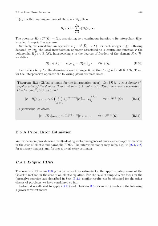
B.5 A Priori Error Estimation 479
If ϕi is the Lagrangian basis of the space X1h, then
Π1hv(x) =
Nh∑
i=1
v(Ni)ϕi(x).
The operator Π1h : C0(Ω) → X1
h, associating to a continuous function v its interpolant Π1hv,
is called interpolation operator.Similarly, we can define an operator Πr
h : C0(Ω) → Xrh, for each integer r ≥ 1. Having
denoted by ΠrK the local interpolation operator associated to a continuous function v the
polynomial ΠrKv ∈ Pr(K), interpolating v in the degrees of freedom of the element K ∈ Th,
we define
Πrhv ∈ Xr
h : Πrhv∣∣K
= ΠrK(v
∣∣K
) ∀K ∈ Th. (B.33)
Let us denote by hK the diameter of each triangle K, so that hK ≤ h for all K ∈ Th. Then,for the interpolation operator the following global estimate holds:
Theorem B.3 (Global estimate for the interpolation error). Let Thh>0 be a family ofregular grids of the domain Ω and let m = 0, 1 and r ≥ 1. Then there exists a constantC = C(r,m, K) > 0 such that
|v −Πrhv|Hm(Ω) ≤ C
( ∑
K∈Th
h2(r+1−m)K |v|2Hr+1(K)
)1/2
∀v ∈ Hr+1(Ω). (B.34)
In particular, we obtain
|v −Πrhv|Hm(Ω) ≤ C hr+1−m|v|Hr+1(Ω) ∀v ∈ Hr+1(Ω). (B.35)
B.5 A Priori Error Estimation
We furthermore provide some results dealing with convergence of finite element approximationsin the case of elliptic and parabolic PDEs. The interested reader may refer, e.g., to [224, 218]for a deeper analysis and further a priori error estimates.
B.5.1 Elliptic PDEs
The result of Theorem B.3 provides us with an estimate for the approximation error of theGalerkin method in the case of an elliptic equation. For the sake of simplicity we focus on the(strongly) coercive case described in Sect. B.2.1; similar results can be obtained for the otherclasses of problems we have considered so far.
Indeed, it is sufficient to apply (B.11) and Theorem B.3 (for m = 1) to obtain the followinga priori error estimate:
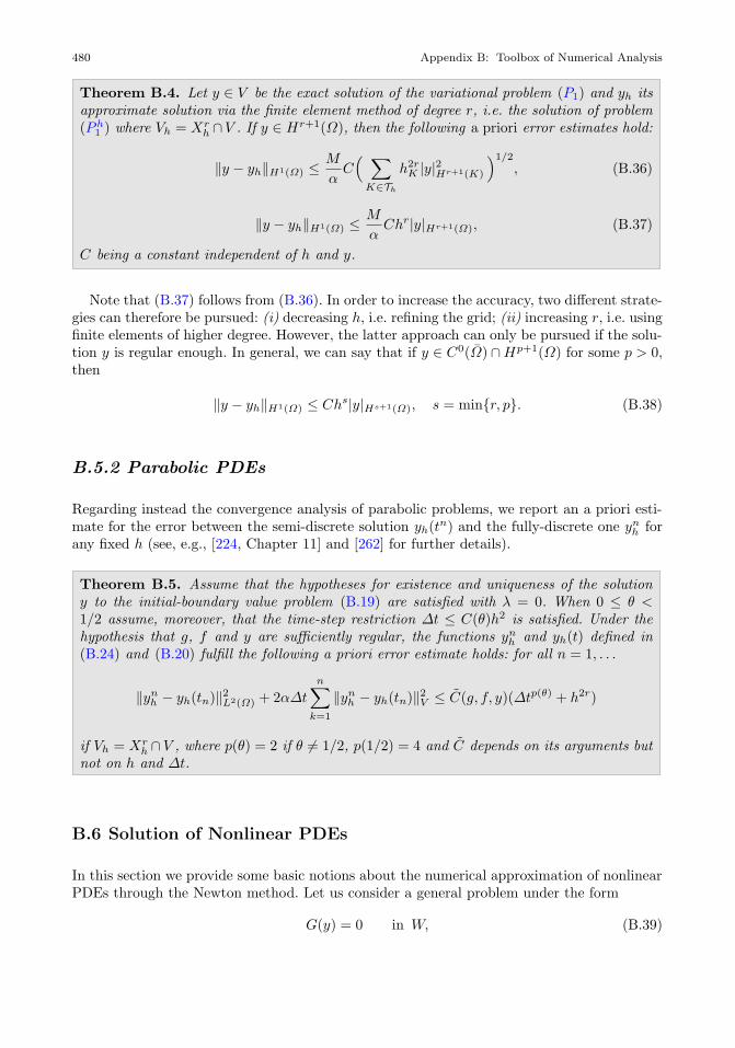
480 Appendix B: Toolbox of Numerical Analysis
Theorem B.4. Let y ∈ V be the exact solution of the variational problem (P1) and yh itsapproximate solution via the finite element method of degree r, i.e. the solution of problem(Ph1 ) where Vh = Xr
h ∩V . If y ∈ Hr+1(Ω), then the following a priori error estimates hold:
‖y − yh‖H1(Ω) ≤M
αC( ∑
K∈Th
h2rK |y|2Hr+1(K)
)1/2
, (B.36)
‖y − yh‖H1(Ω) ≤M
αChr|y|Hr+1(Ω), (B.37)
C being a constant independent of h and y.
Note that (B.37) follows from (B.36). In order to increase the accuracy, two different strate-gies can therefore be pursued: (i) decreasing h, i.e. refining the grid; (ii) increasing r, i.e. usingfinite elements of higher degree. However, the latter approach can only be pursued if the solu-tion y is regular enough. In general, we can say that if y ∈ C0(Ω) ∩Hp+1(Ω) for some p > 0,then
‖y − yh‖H1(Ω) ≤ Chs|y|Hs+1(Ω), s = minr, p. (B.38)
B.5.2 Parabolic PDEs
Regarding instead the convergence analysis of parabolic problems, we report an a priori esti-mate for the error between the semi-discrete solution yh(tn) and the fully-discrete one ynh forany fixed h (see, e.g., [224, Chapter 11] and [262] for further details).
Theorem B.5. Assume that the hypotheses for existence and uniqueness of the solutiony to the initial-boundary value problem (B.19) are satisfied with λ = 0. When 0 ≤ θ <1/2 assume, moreover, that the time-step restriction ∆t ≤ C(θ)h2 is satisfied. Under thehypothesis that g, f and y are sufficiently regular, the functions ynh and yh(t) defined in(B.24) and (B.20) fulfill the following a priori error estimate holds: for all n = 1, . . .
‖ynh − yh(tn)‖2L2(Ω) + 2α∆t
n∑
k=1
‖ynh − yh(tn)‖2V ≤ C(g, f, y)(∆tp(θ) + h2r)
if Vh = Xrh ∩V , where p(θ) = 2 if θ 6= 1/2, p(1/2) = 4 and C depends on its arguments but
not on h and ∆t.
B.6 Solution of Nonlinear PDEs
In this section we provide some basic notions about the numerical approximation of nonlinearPDEs through the Newton method. Let us consider a general problem under the form
G(y) = 0 in W, (B.39)
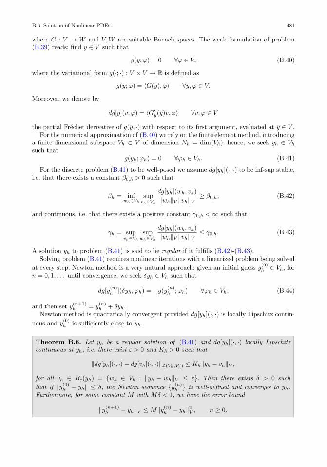
B.6 Solution of Nonlinear PDEs 481
where G : V → W and V,W are suitable Banach spaces. The weak formulation of problem(B.39) reads: find y ∈ V such that
g(y;ϕ) = 0 ∀ϕ ∈ V, (B.40)
where the variational form g(·; ·) : V × V → R is defined as
g(y;ϕ) = 〈G(y), ϕ〉 ∀y, ϕ ∈ V.
Moreover, we denote by
dg[y](v, ϕ) = 〈G′y(y)v, ϕ〉 ∀v, ϕ ∈ V
the partial Frechet derivative of g(y, ·) with respect to its first argument, evaluated at y ∈ V .For the numerical approximation of (B.40) we rely on the finite element method, introducing
a finite-dimensional subspace Vh ⊂ V of dimension Nh = dim(Vh): hence, we seek yh ∈ Vhsuch that
g(yh;ϕh) = 0 ∀ϕh ∈ Vh. (B.41)
For the discrete problem (B.41) to be well-posed we assume dg[yh](·, ·) to be inf-sup stable,i.e. that there exists a constant β0,h > 0 such that
βh = infwh∈Vh
supvh∈Vh
dg[yh](wh, vh)
‖wh‖V ‖vh‖V≥ β0,h, (B.42)
and continuous, i.e. that there exists a positive constant γ0,h <∞ such that
γh = supvh∈Vh
supwh∈Vh
dg[yh](wh, vh)
‖wh‖V ‖vh‖V≤ γ0,h. (B.43)
A solution yh to problem (B.41) is said to be regular if it fulfills (B.42)-(B.43).Solving problem (B.41) requires nonlinear iterations with a linearized problem being solved
at every step. Newton method is a very natural approach: given an initial guess y(0)h ∈ Vh, for
n = 0, 1, . . . until convergence, we seek δyh ∈ Vh such that
dg[y(n)h ](δyh, ϕh) = −g(y
(n)h ;ϕh) ∀ϕh ∈ Vh, (B.44)
and then set y(n+1)h = y
(n)h + δyh.
Newton method is quadratically convergent provided dg[yh](·, ·) is locally Lipschitz contin-
uous and y(0)h is sufficiently close to yh.
Theorem B.6. Let yh be a regular solution of (B.41) and dg[yh](·, ·) locally Lipschitzcontinuous at yh, i.e. there exist ε > 0 and Kh > 0 such that
‖dg[yh](·, ·)− dg[vh](·, ·)‖L(Vh,V ′h) ≤ Kh‖yh − vh‖V ,
for all vh ∈ Bε(yh) = wh ∈ Vh : ‖yh − wh‖V ≤ ε. Then there exists δ > 0 such
that if ‖y(0)h − yh‖ ≤ δ, the Newton sequence y(n)
h is well-defined and converges to yh.Furthermore, for some constant M with Mδ < 1, we have the error bound
‖y(n+1)h − yh‖V ≤M‖y(n)
h − yh‖2V , n ≥ 0.
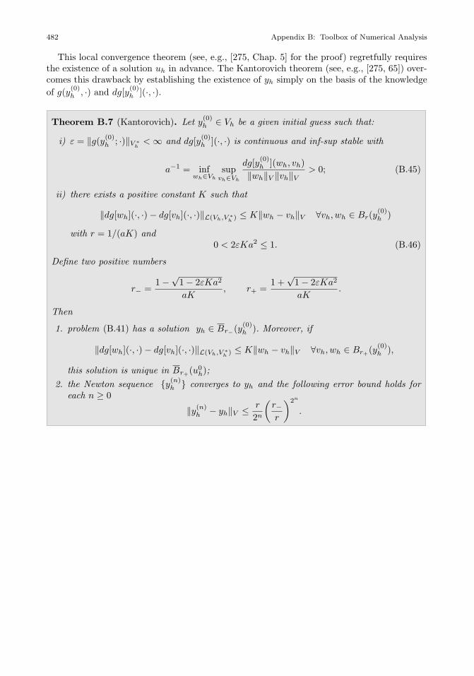
482 Appendix B: Toolbox of Numerical Analysis
This local convergence theorem (see, e.g., [275, Chap. 5] for the proof) regretfully requiresthe existence of a solution uh in advance. The Kantorovich theorem (see, e.g., [275, 65]) over-comes this drawback by establishing the existence of yh simply on the basis of the knowledge
of g(y(0)h , ·) and dg[y
(0)h ](·, ·).
Theorem B.7 (Kantorovich). Let y(0)h ∈ Vh be a given initial guess such that:
i) ε = ‖g(y(0)h ; ·)‖V ∗h <∞ and dg[y
(0)h ](·, ·) is continuous and inf-sup stable with
a−1 = infwh∈Vh
supvh∈Vh
dg[y(0)h ](wh, vh)
‖wh‖V ‖vh‖V> 0; (B.45)
ii) there exists a positive constant K such that
‖dg[wh](·, ·)− dg[vh](·, ·)‖L(Vh,V ∗h ) ≤ K‖wh − vh‖V ∀vh, wh ∈ Br(y(0)h )
with r = 1/(aK) and0 < 2εKa2 ≤ 1. (B.46)
Define two positive numbers
r− =1−√
1− 2εKa2
aK, r+ =
1 +√
1− 2εKa2
aK.
Then
1. problem (B.41) has a solution yh ∈ Br−(y(0)h ). Moreover, if
‖dg[wh](·, ·)− dg[vh](·, ·)‖L(Vh,V ∗h ) ≤ K‖wh − vh‖V ∀vh, wh ∈ Br+(y(0)h ),
this solution is unique in Br+(u0h);
2. the Newton sequence y(n)h converges to yh and the following error bound holds for
each n ≥ 0
‖y(n)h − yh‖V ≤
r
2n
(r−r
)2n
.
References
1. F. Abergel and R. Temam. On some control problems in fluid mechanics. Theoret. Comput. Fluid
Dynamics, 1:303–325, 1990.
2. V.I. Agoshkov, D. Ambrosi, V. Pennati, A. Quarteroni, and F. Saleri. Mathematical and numericalmodelling of shallow water flow. Comput. Mech., 11(5):280–299, 1993.
3. M. Ainsworth and J. T. Oden. A Posteriori Error Estimation in Finite Element Analysis. Wiley-
Interscience, 2000.4. V. Akcelik, G. Biros, O. Ghattas, J. Hill, D. Keyes, and B. Waanders. Parallel Algorithms for PDE-
Constrained Optimization. In M.A. Heroux, P. Raghavan, and H.D. Simon, editors, Parallel Processingfor Scientific Computing, Philadelphia, PA, USA, 2006. Society for Industrial and Applied Mathematics.
5. R. R. Aliev and A. V. Panfilov. A simple two-variable model of cardiac excitation. Chaos Soliton Fract.,7(3):293–301, 1996.
6. G. Allaire. Conception optimale de structures. Springer Verlag, 2007. Vol. 58 Mathematiques et Appli-
cations.7. G. Allaire, F. de Gournay, F. Jouve, and A.-M. Toader. Structural optimization using topological and
shape sensitivity via a level-set method. Control and Cybernetics, 34(1):59–80, 2005.
8. G. Allaire, F. Jouve, and A.-M. Toader. Structural optimization using sensitivity analysis and a level-setmethod. J. Comput. Phys., 194(1):363–393, 2004.
9. G. Allaire and O. Pantz. Structural optimization with freefem++. Struct. Multidisc. Optim., 32(3):173–
181, 2006.10. W. Alt. The Lagrange-Newton method for infinite-dimensional optimization problems. Numer. Funct.
Anal. Optim., 11(3-4):201–224, 1990.
11. W. Alt and K. Malanowski. The Lagrange-Newton method for nonlinear optimal control problems.Comput. Optim. Appl., 2(1):77–100, 1993.
12. E.I. Amoiralis and I.K. Nikolos. Freeform deformation versus B-spline representation in inverse airfoil
design. J. Comput. Inf. Sci. Engrg., 8(2), 2008.13. J.S. Arora and Q. Wang. Review of formulations for structural and mechanical system optimization.
Struct. Multidisc. Optim., 30(4):251–272, 2005.14. M. Asch, M. Bocquet, and M. Nodet. Data Assimilation: Methods, Algorithms, and Applications. SIAM,
2016.15. K.J. Astrom and R.M. Murray. Feedback systems: an introduction for scientists and engineers. Princeton
University Press, 2010.16. I. Babuska. The finite element method with lagrangian multipliers. Numer. Math., 20:179–192, 1973.
17. F. Ballarin, A. Manzoni, G. Rozza, and S. Salsa. Shape optimization by free-form deformation: existence
results and numerical solution for stokes flows. J. Sci. Comput., 60(3):537–563, 2014.18. H.T. Banks and K. Kunisch. The linear regulator problem for parabolic systems. SIAM J. Control
Optim., 22(5):684–698, 1984.
19. V. Barbu. Feedback control of time dependent stokes flows. In S.S. Sritharan, editor, Optimal Controlof Viscous Flow, chapter 3, pages 63–77. Society for Industrial and Applied Mathematics, Philadelphia,
PA, USA, 1998.20. R.A. Bartlett, M. Heinkenschloss, D. Ridzal, and B. van Bloemen Waanders. Domain decomposition
methods for advection dominated linear-quadratic elliptic optimal control problems. Comput. Meth.Appl. Mech. Engrg., 195(44?-47):6428–6447, 2006.
21. G. Basile and G. Marro. Controlled and Conditioned Invariants in Linear System Theory. Prentice HallEnglewood Cliffs, NJ, 1992.
483© Springer Nature Switzerland AG 2021
A. Manzoni et al., Optimal Control of Partial Differential Equations,
Applied Mathematical Sciences 207, https://doi.org/10.1007/978-3-030-77226-0

484 References
22. A. Battermann and M. Heinkenschloss. Preconditioners for karush-kuhn-tucker matrices arising in the
optimal control of distributed systems. In Control and Estimation of Distributed Parameter Systems,pages 15–32. Springer, 1998.
23. R. Becker, H. Kapp, and R. Rannacher. Adaptive finite element methods for optimal control of partialdifferential equations: Basic concepts. SIAM, J. Control Opt., 39(1):113–132, 2000.
24. R. Becker and R. Rannacher. A feed-back approach to error control in finite element method: Basic
analysis and examples. East - West J. Numer. Math., 4:237–264, 1996.
25. R. Becker and R. Rannacker. An optimal control approach to a posteriori error estimation in finiteelement methods. Acta Numerica, pages 1–102, 2001.
26. J.A. Bello, E. Fernandez-Cara, J. Lemoine, and J. Simon. The differentiability of the drag with respectto the variations of a Lipschitz domain in a Navier-Stokes flow. SIAM J. Control. Optim., 35(2):626–640,1997.
27. M.P. Bendsoe and O. Sigmund. Topology optimization theory, methods and applications. Springer-Verlag,Berlin Heidelberg, 2004.
28. P. Benner, S. Gorner, and J. Saak. Numerical solution of optimal control problems for parabolic systems.
In Parallel Algorithms and Cluster Computing, volume 52 of Lecture Notes in Computational Scienceand Engineering, pages 151–169. Springer, Berlin, Heidelberg, 2006.
29. M. Benzi, L. Ferragut, M. Pennacchio, and V. Simoncini. Solution of linear systems from an optimalcontrol problem arising in wind simulation. Numerical Linear Algebra with Applications, 17(6):895–915,2010.
30. M. Benzi, G.H. Golub, and J. Liesen. Numerical solution of saddle point problems. Acta Numerica,
14:1–137, 2005.31. M. Benzi and M. A. Olshanskii. An augmented lagrangian-based approach to the oseen problem. SIAM
J. Sci. Comput., 28(6):2095–2113, 2006.32. M. Berggren. Numerical solution of a flow-control problem: vorticity reduction by dynamic boundary
action. SIAM J. Sci. Comput., 19(3):829–860, 1998.
33. M. Berggren. Approximations of very weak solutions to boundary-value problems. SIAM J. Numer.Anal., 42(2):860–877, 2004.
34. M. Bergounioux, K. Ito, and K. Kunisch. Primal-dual strategy for constrained optimal control problems.SIAM J. Control Optim., 237(4):1176–1194, 1999.
35. M. Bergounioux and K. Kunisch. Primal-dual strategy for state-constrained optimal control problems.
Comput. Optim. Appl., 22(2):193–224, 2002.
36. D.P. Bertsekas. Constrained optimization and Lagrange multiplier methods. Academic Press, New York,1982.
37. J.T. Betts. Practical methods for optimal control and estimation using nonlinear programming. SIAM,
2010.38. G. Biros and O. Ghattas. Parallel lagrange–newton–krylov–schur methods for pde-constrained optimiza-
tion. part ii: The lagrange–newton solver and its application to optimal control of steady viscous flows.SIAM J. Sci. Comput., 27(2):714–739, 2005.
39. G. Biros and O. Ghattas. Parallel lagrange-newton-krylov-schur methods for pde- constrained optimiza-tion. part i: The krylov-schur solver. SIAM J. Sci. Comput., 27:687–713, 2005.
40. A. Bjorck. Numerical Methods in Matrix Computations, volume 59 of Texts in Applied Mathematics.
Springer International Publishing, Switzerland, 2015.
41. D. Boffi, F. Brezzi, and M. Fortin. Mixed Finite Elements and Applications. Springer-Verlag, Berlin-Heidelberg, 2013.
42. A. Borzı and K. Kunisch. A multigrid scheme for elliptic constrained optimal control problems. Comput.
Optim. Appl., 31:309–333, 2005.43. A. Borzı and V. Schulz. Multigrid methods for PDE optimization. SIAM Review, 51(2):361–395, 2009.
44. A. Borzı and V. Schulz. Computational optimization of systems governed by partial differential equations.
Society for Industrial and Applied Mathematics, Philadephia, PA, 2011.45. M. Boulakia, M.A Fernandez, J.F. Gerbeau, and N. Zemzemi. A coupled system of pdes and odes arising
in electrocardiograms modeling. Applied Math. Res. Exp., 28(2008(abn002)), 2008.46. Y. Bourgault, Y. Coudiere, and C. Pierre. Existence and uniqueness of the solution for the bidomain
model used in cardiac electrophysiology. Nonlinear analysis: Real world applications, 10(1):458–482,
2009.47. J. Boyle, M. D. Mihajlovic, and J. A. Scott. HSL MI20: an efficient AMG preconditioner, 2007.
48. D. Braess and P. Peisker. On the numerical solution of the Biharmonic equation and the role of squaring
matrices for preconditioning. IMA J. Numer. Anal., 6(4):393–404, 1986.49. J. H. Bramble and J. E. Pasciak. A preconditioning technique for indefinite systems resulting from mixed
approximations of elliptic problems. Math. Comp., 50:1–17, 1988.
50. J.H. Bramble. Multigrid Methods. Pitman Research Notes in Mathematics Series, Essex, 1993.
References 485
51. C. Brandenburg, F. Lindemann, M. Ulbrich, and S. Ulbrich. A continuous adjoint approach to shapeoptimization for Navier Stokes flow. In K. Kunisch, J. Sprekels, G. Leugering, and F. Troltzsch, editors,Optimal Control of Coupled Systems of Partial Differential Equations, volume 158 of International Series
of Numerical Mathematics, pages 35–56. Birkhauser Verlag, 2009.52. H. Brezis. Functional Analysis, Sobolev Spaces and Partial Differential Equations. Springer-Verlag, New
York, 2011.53. F. Brezzi. On the existence, uniqueness, and approximation of saddle point problems arising from La-
grangian multipliers. R.A.I.R.O., Anal. Numer., 2:129–151, 1974.54. A. E. Bryson and Y.-C. Ho. Applied optimal control: optimization, estimation and control. CRC Press,
1975.55. M. Cannon, C. Cullum, and E. Polak. Theory and Optimal Control and Mathematical Programming.
McGraw-Hill, New York, 1970.56. Y. Cao, S. Li, L. Petzold, and R. Serban. Adjoint sensitivity analysis for differential-algebraic equations:
The adjoint dae system and its numerical solution. SIAM J. Sci. Comput., 24(3):1076–1089, 2003.57. H. Cartan. Calcul Differentiel. Hermann, Paris, 1967.58. E. Casas and F. Troltzsch. Error estimates for linear-quadratic elliptic control problems. In V. Barbu et
al., editor, Analysis and optimization of differential systems, pages 89–100. Springer, 2003.59. E. Casas and F. Troltzsch. Second order optimality conditions and their role in pde control. Jahresber.
Dtsch. Math. Ver., 117(1):3–44, 2015.60. J. Cea. Conception optimale ou identification de formes: calcul rapide de la derivee directionelle de la
fonction cout. Mathematical Modelling and Numerical Analysis, 20(3):371–402, 1986.61. J. Cea, S. Garreau, P. Guillaume, and M. Masmoudi. The shape and topological optimizations connection.
Comput. Methods Appl. Mech. Engrg., 188:713–726, 2000.62. N. Chamakuri, K. Kunisch, and G. Plank. Numerical solution for optimal control of the reaction-diffusion
equations in cardiac electrophysiology. Comput. Optim. Appl., 49:149–178, 2011.63. K. Chrysafinos and S. Hou. Analysis and approximation of the evolutionary Stokes equations with
inhomogeneous boundary and divergence data using a parabolic saddle point formulation. ESAIM:
Math. Model. Numer. Anal., 51:1501–1526, 2017.64. P. G. Ciarlet. The Finite Element Method for Elliptic Problems. Classics in Applied Mathematics, 40.
Society for Industrial and Applied Mathematics, Philadephia, PA, 2002.65. P. G. Ciarlet. Linear and nonlinear functional analysis with applications. Society for Industrial and
Applied Mathematics, Philadelphia, 2014.66. P. Clement. Approximation by finite element functions using local regularization. RAIRO, Anal. Num.,
9:77–84, 1975.67. P. Colli Franzone and L. F. Pavarino. A parallel solver for reaction–diffusion systems in computational
electrocardiology. Math. Mod. Meth. Appl. Sci., 14(06):883–911, 2004.68. P. Colli Franzone, L.F. Pavarino, and S. Scacchi. Mathematical cardiac electrophysiology, volume 13 of
Modeling, Simulation and Applications (MS&A) Series. Springer-Verlag Italia, Milano, 2014.69. Piero Colli Franzone, Peter Deuflhard, Bodo Erdmann, Jens Lang, and Luca F Pavarino. Adaptivity in
space and time for reaction-diffusion systems in electrocardiology. SIAM J. Sci. Comput., 28(3):942–962,
2006.70. A. R. Conn, N. I. M. Gould, and P. L. Toint. Trust Region Methods. Society for Industrial and Applied
Mathematics, Philadelphia, PA, USA, 2000.71. A. R. Conn, K. Scheinberg, and L. N. Vicente. Introduction to Derivative-Free Optimization. Society for
Industrial and Applied Mathematics, Philadelphia, PA, USA, 2009.72. J.-M. Coron. Control and Nonlinearity. American Mathematical Society, 2007.73. R. Dautray and J. L. Lions. Mathematical Analysis and Numerical Methods for Science and Technology.
Springer-Verlag, Berlin Heidelberg, 2000.74. J.C. de los Reyes and K. Kunisch. A semi-smooth newton method for control constrained boundary
optimal control of the navier-stokes equations. Nonlinear Analysis, 62(7):1289–1316, 2005.75. K. Deckelnick, A. Gunther, and M. Hinze. Finite element approximation of dirichlet boundary control for
elliptic pdes on two-and three-dimensional curved domains. SIAM J. Control Optim., 48(4):2798–2819,
2009.76. K. Deckelnick and M. Hinze. Numerical analysis of a control and state constrained elliptic control
problem with piecewise constant control approximations. In K. Kunisch, G. Of, and O. Steinbach, editors,
Numerical Mathematics and Advanced Applications, pages 597–604. Springer, Berlin, Heidelberg, 2008.77. L. Dede. Optimal flow control for Navier-Stokes equations: Drag minimization. Int. J. Numer. Meth.
Fluids, 55(4):347 – 366, 2007.78. L. Dede and A. Quarteroni. Optimal control and numerical adaptivity for advection–diffusion equations.
ESAIM Math. Modelling Numer. Anal., 39(5):1019–1040, 2005.79. M.C. Delfour and J.P. Zolesio. Shapes and geometries - analysis, differential calculus, and optimization.
Society for Industrial and Applied Mathematics, Philadephia, PA, 2nd edition, 2011.
486 References
80. J. Dennis and R. Schnabel. Numerical Methods for Unconstrained Optimization and Nonlinear Equations.
Classics in Applied Mathematics. Society for Industrial and Applied Mathematics (SIAM), Philadelphia,PA, 1996.
81. M. Desai and K. Ito. Optimal controls of Navier–Stokes equations. SIAM J. Control Optim., 32(5):1428–1446, 1994.
82. J.A. Desideri, B. Abou El Majd, and A. Janka. Nested and self-adaptive Bezier parameterizations forshape optimization. J. Comput. Phys., 224(1):117–131, 2007.
83. H. Do, A. A. Owida, and Y. S. Morsi. Numerical analysis of coronary artery bypass grafts: An over view.Comput. Meth. Prog. Bio., 108:689–705, 2012.
84. H. S. Dollar, N. I. M. Gould, W. H. A. Schilders, and A. J. Wathen. Implicit-factorization preconditioningand iterative solvers for regularized saddle-point systems. SIAM J. Matrix Anal. Appl., 28:170–189, 2006.
85. H. S. Dollar, N. I. M. Gould, W. H. A. Schilders, and A. J. Wathen. Using constraint preconditionerswith regularized saddle-point problems. Computational Optimization and Applications, 36(2):249–270,2007.
86. H.S. Dollar, N.I.M. Gould, M. Stoll, and A.J. Wathen. Preconditioning Saddle-Point Systems withApplications in Optimization. SIAM J. Sci. Comput., 32:249–270, February 2010.
87. H. Elman, V. E. Howle, J. Shadid, R. Shuttleworth, and R. Tuminaro. Block preconditioners based onapproximate commutators. SIAM J. Sci. Comput., 27(5):1651–1668, 2006.
88. H. C. Elman, D. J. Silvester, and A.J. Wathen. Finite Elements and Fast Iterative Solvers with Appli-cations in Incompressible Fluid Dynamics. Oxford University Press, New York, 2004.
89. H.C.. Elman and G.H. Golub. Inexact and preconditioned Uzawa algorithms for saddle point problems.SIAM J. Numer. Anal., 6:1645–1661, 1994.
90. H.C. Elman, D.J. Silvester, and A.J. Wathen. Finite Elements and Fast Iterative Solvers with Applica-tions in Incompressible Fluid Dynamics. Oxford Science Publications, Series in Numerical Mathematicsand Scientific Computation, Clarendon Press, Oxford, 2005.
91. H.W. Engl, M. Hanke, and A. Neubauer. Regularization of Inverse Problems. Mathematics and itsApplications. Kluwer Academic Publisher, Dordrecht, The Netherlands, 2000.
92. S. Ervedoza and E. Zuazua. The Wave Equation: Control and Numerics, pages 245–339. Springer BerlinHeidelberg, 2012.
93. S. Ervedoza and E. Zuazua. Numerical Approximation of Exact Controls for Waves. SpringerBriefs inMathematics. Springer-Verlag New York, 2013.
94. R. S. Falk. Approximation of a class of optimal control problems with order of convergence estimates. J.
Math. Anal. Appl., 44:28–47, 1973.95. R. Fletcher. Practical methods of optimization. Wiley-Interscience (John Wiley & Sons), New York, 2nd
edition, 2001.
96. A. V. Fursikov. Optimal Control of Distributed Systems. Theory and Applications. American Mathe-matical Society, 1999.
97. A. V. Fursikov, M. D. Gunzburger, and L. S. Hou. Boundary value problems and optimal boundarycontrol for the navier–stokes system: the two-dimensional case. SIAM J. Control Optim., 36(3):852–894,
1998.
98. A.V. Fursikov and R. Rannacher. Optimal Neumann control for the two-dimensional steady-state Navier-Stokes equations. In A.V. Fursikov, G. P. Galdi, and V.V. Pukhnachev, editors, New Directions in
Mathematical Fluid Mechanics: The Alexander V. Kazhikhov Memorial Volume. Birkhauser Basel, Basel,
2010.99. J. Gain and D. Bechmann. A survey of spatial deformation from a user-centered perspective. ACM
Trans. Graph., 27(4):107:1–107:21, 2008.
100. Z. Gao and Y. Ma. A new stabilized finite element method for shape optimization in the steady navier–stokes flow. Appl. Num. Math., 60(8):816–832, 2010.
101. Z. Gao, Y. Ma, and H. Zhuang. Drag minimization for navier–stokes flow. Numerical Methods for Partial
Differential Equations, 25(5):1149–1166, 2009.102. T. Geveci. On the approximation of the solution of an optimal control problem governed by an elliptic
equation. R.A.I.R.O., Anal. Numer., 13(4):313–328, 1978.103. O. Ghattas and J.H. Bark. Optimal control of two- and three-dimensional incompressible Navier-Stokes
flows. J. Comput. Phys., 136(2):231–244, 1997.
104. D. Gilbarg and N.S. Trudinger. Elliptic Partial Differential Equations of Second Order. Springer Verlag,Berlin, 1983.
105. V. Girault and P.-A. Raviart. Finite element methods for Navier-Stokes equations: Theory and algo-
rithms. Springer-Verlag, Berlin and New York, 1986.106. G.H. Golub and C.F. Van Loan. Matrix computations (3rd ed.). Johns Hopkins University Press, 1996.
107. W. Gong, M. Hinze, and Z. Zhou. Finite element method and a priori error estimates for dirichlet
boundary control problems governed by parabolic pdes. J. Sci. Comput., 66(3):941–967, 2016.
References 487
108. W. Gong and N. Yan. A posteriori error estimate for boundary control problems governed by the parabolicpartial differential equations. J. Comput. Math., pages 68–88, 2009.
109. Wei Gong, Michael Hinze, and Zhaojie Zhou. A priori error analysis for finite element approximation of
parabolic optimal control problems with pointwise control. SIAM J. Control Optim., 52(1):97–119, 2014.110. N. Gould and V. Simoncini. Spectral analysis of saddle point matrices with indefinite leading blocks.
SIAM J. Matrix Anal. & Appl., 31(3):1152–1171, 2009.111. N. I. M. Gould, M. E. Hribar, and J. Nocedal. On the solution of equality constrained quadratic pro-
gramming problems arising in optimization. SIAM J. Sci. Comput., 23:1376–1395, 2001.112. T. Gratsch and K. J. Bathe. A posteriori error estimation techniques in practical finite element analysis.
Comput. and Struct., 83:235–265, 2005.113. P.M. Gresho and R.L. Sani. Incompressible Flow and the Finite Element Method: Advection-Diffusion
and Isothermal Laminar Flow. John Wiley & Sons, 1998.114. J.A. Griepentrog and L. Recke. Linear elliptic boundary value problems with non-smooth data: Normal
solvability on sobolev-campanato spaces. Mathematische Nachrichten, 225(1):39–74, 2001.115. J. A Griepentrop. Linear elliptic boundary value problems with nonsmooth data: Campanato spaces of
functionals. Math. Nachr., 243:19–42, 2002.116. R. Griesse and B. Vexler. Numerical sensitivity analysis for the quantity of interest in pde-constrained
optimization. SIAM J. Sci. Comput., 29:22–48, January 2007.117. R. Griesse and S. Volkwein. A primal-dual active set strategy for optimal boundary control of a nonlinear
reaction-diffusion system. SIAM J. Control Optim., 44(2):467–494, 2005.118. P. Grisvard. Elliptic problems in nonsmooth domains. SIAM, 2011.119. M. Gunzburger, L. Hou, and T. P. Svobodny. Analysis and finite element approximation of optimal
control problems for the stationary Navier-Stokes equations with distributed and Neumann controls.Math. Comp., 57:123–151, 1991.
120. M. D. Gunzburger. Sensitivities, adjoints and flow optimization. Int. J. Numer. Methods Fluids, 31(1):53–
78, 1999.121. M. D. Gunzburger and P.B. Bochev. Least-Squares Finite Element Methods. Springer-Verlag, New York,
2009.122. M. D. Gunzburger and S. Manservisi. The velocity tracking problem for navier–stokes flows with bounded
distributed controls. SIAM J. Control Optim., 37(6):1913–1945, 1999.123. M. D. Gunzburger and S. Manservisi. Analysis and approximation of the velocity tracking problem for
navier–stokes flows with distributed control. SIAM J. Numer. Anal., 37(5):1481–1512, 2000.124. M. D. Gunzburger and S. Manservisi. The velocity tracking problem for navier–stokes flows with boundary
control. SIAM J. Control Optim., 39(2):594–634, 2000.125. Max D. Gunzburger and Steven L. Hou. Treating inhomogeneous essential boundary conditions in finite
element methods and the calculation of boundary stresses. SIAM J. Numer. Anal., 29(2):390–424, 1992.126. M.D. Gunzburger and P.B. Bochev. Least-squares finite element methods for optimization and control
problems for the Stokes equations. Comput. Math. with Appl., 48(7–8):1035–1057, 2004.127. M.D. Gunzburger, L. Hou, and T.P. Svobodny. Boundary velocity control of incompressible flow with an
application to viscous drag reduction. SIAM J. Control Optim., 30:167–181, 1992.128. M.D. Gunzburger, L. S. Hou, and Th. P. Svobodny. Analysis and finite element approximation of optimal
control problems for the stationary navier-stokes equations with dirichlet controls. ESAIM: Math. Model.
Numer. Anal., 25(6):711–748, 1991.129. M.D. Gunzburger, L.S. Hou, and T.P. Svobodny. Optimal control problems for a class of nonlinear
equations with an application to control of fluids. In S.S. Sritharan, editor, Optimal Control of Viscous
Flow, pages 43–62. Society for Industrial and Applied Mathematics, 1998.130. M.D. Gunzburger and H. Kim. Existence of an optimal solution of a problem for the stationary Navier-
Stokes equations. SIAM J. Control Optim., 36(3):895–909, 1998.131. E. Haber and U. Ascher. Preconditioned all-at-once methods for large sparse parameter estimation
problems. Inverse Problems, 17:1847–1864, 2000.132. W. Hackbusch. Multi-grid Methods and Applications. Springer-Verlag, New York, 1985.133. R. Haller-Dintelmann, C. Meyer, J. Rehberg, and A. Schiela. Holder continuity and optimal control for
nonsmooth elliptic problems. Applied Mathematics & Optimization, 60(3):397–428, 2009.134. J. Haslinger and R. A. E. Makinen. Introduction to Shape Optimization: Theory, Approximation, and
Computation. Society for Industrial and Applied Mathematics, Philadephia, PA, 2003.135. J. Haslinger and P. Neittaanmaki. Finite element approximation for optimal shape, material and topology
design (2nd Ed). Wiley & Sons, 2nd edition, 1996.136. X. He and C. Vuik. Comparison of some preconditioners for the incompressible navier-stokes equations.
Numer. Math. Theor. Meth. Appl., 9(2):239–261, 2016.137. M. Heinkenschloss. Formulation and analysis of a sequential quadratic programming method for the
optimal dirichlet boundary control of Navier-Stokes flow. In Optimal Control: Theory, Algorithms, and
Applications, pages 178–203. Springer US, 1998.
488 References
138. M. Heinkenschloss and H. Nguyen. Neumann-neumann domain decomposition preconditioners for linear-quadratic elliptic optimal control problems. SIAM J. Sci. Comput., 28(3):1001–1028, 2006.
139. A. Henrot and M. Pierre. Variation et optimisation de formes. Une analyse geometrique, volume 48 of
Series Mathematiques et Applications. Springer, 2005.
140. R. Herzog and K. Kunisch. Algorithms for pde-constrained optimization. GAMM-Mitteilungen,33(2):163–176, 2010.
141. R. Herzog and E. Sachs. Preconditioned conjugate gradient method for optimal control problems withcontrol and state constraints. SIAM. J. Matrix Anal. Appl., 31:2291–2317, 2010.
142. M. Hintermuller and M. Hinze. Moreau-yosida regularization in state constrained elliptic control prob-lems: Error estimates and parameter adjustment. SIAM J. Numer. Anal., 47(3):1666–1683, 2009.
143. M. Hintermuller, K. Ito, and K. Kunisch. The primal-dual active set strategy as a semismooth newtonmethod. SIAM J. Optim., 13(3):865–888, 2002.
144. M. Hintermuller, K. Kunisch, Y. Spasov, and S. Volkwein. Dynamical systems-based optimal control ofincompressible fluids. Int. J. Numer. Meth. Fluids, 46(4):345–359, 2004.
145. M. Hinze. A variational discretization concept in control constrained optimization: the linear-quadraticcase. Comput. Optim. Appl., 30(1):45–61, 2005.
146. M. Hinze and K. Kunisch. Second order methods for optimal control of time-dependent fluid flow. SIAM
J. Control Optim., 40(3):925–946, 2001.
147. M. Hinze and C. Meyer. Variational discretization of lavrentiev-regularized state constrained ellipticoptimal control problems. Comput. Optim. Appl., 46(3):487–510, 2010.
148. M. Hinze, R. Pinnau, M. Ulbrich, and S. Ulbrich. Optimization with PDE Constraints, volume 23 of
Mathematical Modelling: Theory and Applications. Springer, 2009.149. L. S. Hou and S. S. Ravindran. Numerical approximation of optimal flow control problems by a penalty
method: Error estimates and numerical results. SIAM J. Sci. Comput., 20(5):1753–1777, April 1999.150. K. Ito and K. Kunisch. The primal-dual active set method for nonlinear optimal control problems with
bilateral constraints. SIAM J. Control Optim., 43(1):357–376, 2004.
151. K. Ito and K. Kunisch. Lagrange multiplier approach to variational problems and applications. Advancesin design and control. Society for Industrial and Applied Mathematics, 2008.
152. S. Jakobsson and O. Amoignon. Mesh deformation using radial basis functions for gradient-based aero-
dynamic shape optimization. Comput. Fluids, 36:1119–1136, 2007.153. A. Jameson. Aerodynamic design via control theory. J. Sci. Comput., 3:233–260, 1988.
154. J. Kaipio and E. Somersalo. Statistical and computational inverse problems, volume 160 of Applied
Mathematical Sciences. Springer Science+Business Media, Inc., 2005.155. M. I. Kamien and N.L. Schwartz. Dynamic Optimization: The Calculus of Variations and Optimal
Control in Economics and Management, volume 31 of Advanced Textbooks in Economics. North-Holland,
Amsterdam, The Netherlands, 2nd edition, 1991.156. D. Kay, D. Loghin, and A. Wathen. A preconditioner for the steady-state navier–stokes equations. SIAM
J. Sci. Comput., 24(1):237–256, 2002.157. C. Keller, N. I. M. Gould, and A. J. Wathen. Constraint preconditioning for indefinite linear systems.
SIAM J. Matrix Anal. Appl., 21:1300–1317, 2000.
158. H. Kim. A boundary control problem for vorticity minimization in time-dependent 2D Navier-Stokesequations. Korean J. Math., 23(2):293–312, 2006.
159. H. Kim and O.K. Kwon. On a vorticity minimization problem for the stationary 2D Stokes equations.J. Korean Math. Soc., 43(1):45–63, 2006.
160. T. Kim and D. Cao. Non-stationary Navier-Stokes equations with mixed boundary conditions. J. Math.
Sci. Univ. Tokyo, 24:159–194, 2017.
161. K. Kunisch, K. Pieper, and A. Rund. Time optimal control for a reaction diffusion system arising incardiac electrophysiology: a monolithic approach. ESAIM: Math. Model. Numer. Anal., 50(2):381–414,
2016.
162. K. Kunisch and A. Rosch. Primal-dual active set strategy for a general class of constrained optimalcontrol problems. SIAM J. Optim., 13(2):321–334, 2002.
163. K. Kunisch and A. Rund. Time optimal control of the monodomain model in cardiac electrophysiology.IMA J. Appl. Math., 80(6):1664–1683, 2015.
164. K. Kunisch and B. Vexler. Optimal vortex reduction for instationary flows based on translation invariant
cost functionals. SIAM J. Control Optim, 46(4):1368–1397, 2007.165. O. Ladyzhenskaya. The mathematical theory of viscous incompressible flow. Gordon and Breach Science
Publishers, New York, 2nd edition, 1969.
166. J. Lagarias, J. Reeds, M. Wright, and P. Wright. Convergence properties of the Nelder-Mead simplexmethod in low dimensions. SIAM J. Optim., 9(1):112–147, 1999.
167. J. Larson, M. Menickelly, and S. M. Wild. Derivative-free optimization methods. Acta Numerica, 28:287–
404, 2019.
References 489
168. I. Lasiecka and R. Triggiani. Control Theory for Partial Differential Equations: Continuous and Ap-
proximation Theories. I: Abstract Parabolic Systems. Cambridge University Press, 2010.169. T. Lassila, A. Manzoni, A. Quarteroni, and G. Rozza. Boundary control and shape optimization for
the robust design of bypass anastomoses under uncertainty. ESAIM Math. Modelling Numer. Anal.,47(4):1107–1131, 2013.
170. T. Lassila, A. Manzoni, A. Quarteroni, and G. Rozza. A reduced computational and geometrical frame-work for inverse problems in haemodynamics. Int. J. Numer. Methods Biomed. Engng., 29(7):741–776,2013.
171. K. Law, A. Stuart, and K. Zygalakis. Data Assimilation. A Mathematical Introduction, volume 62 ofTexts in Applied Mathematics. Springer International Publishing Switzerland, 2015.
172. E.B. Lee and L. Markus. Foundations of Optimal Control Theory. Krieger Pub. Co., 1986.173. T. Lehnhauser and M. Schafer. A numerical approach for shape optimization of fluid flow domains.
Comput. Methods Appl. Mech. Engrg., 194:5221–5241, 2005.174. R. Li, W. Liu, H. Ma, and T. Tang. Adaptive finite element approximation for distribuited elliptic optimal
control problems. SIAM J. Control Optim., pages 1321–1349, 2001.175. J. L. Lions. Exact controllability, stabilization and perturbations for distributed systems. SIAM Review,
30(1):1–68, 1988.176. J.-L. Lions and E. Magenes. Non-Homogenous Boundary Value Problems and Applications. Springer-
Verlag, 1972.177. J.L. Lions. Optimal Control of Systems governed by Partial Differential Equations. Springer-Verlag,
Berlin Heidelberg, 1971.178. J.L. Lions. Some aspects of the optimal control of distributed parameter systems. Society for Industrial
and Applied Mathematics, Philadelphia, PA, USA, 1972.179. W. Liu, H. Ma, T. Tang, and N. Yan. A posteriori error estimates for discontinuous galerkin time-
stepping method for optimal control problems governed by parabolic equations. SIAM J. Numer. Anal.,
42(3):1032–1061, 2004.180. W. Liu and N. Yan. A posteriori error estimates for some model boundary control problems. J. Comput.
Appl. Math., pages 159–173, 2000.181. W. Liu and N. Yan. A posteriori error estimates for distribuited convex optimal control problems. Adv.
Comput. Math., 15:285–309, 2001.182. W. Liu and N. Yan. A posteriori error estimates for control problems governed by stokes equations.
SIAM J. Numer. Anal., 40(5):1850–1869, 2002.183. W. Liu and N. Yan. A posteriori error estimates for optimal control problems governed by parabolic
equations. Num. Math., 93(3):497–521, 2003.184. D. Luenberger. Introduction to Linear and Non Linear Programming. Addison-Wesley, Reading, Mas-
sachusetts, 1973.185. R. Luus. Iterative Dynamic Programming. Chapman & Hall, 2000.186. J. Macki and A. Strauss. Introduction to Optimal Control Theory. Undergraduate Texts in Mathematics.
Springer-Verlag, New York, 2nd edition, 1982.187. A. Manzoni and S. Pagani. A certified rb method for PDE-constrained parametric optimization problems.
Commun. Appl. Ind. Math., 10(1):123–?152, 2019.188. A. Manzoni, A. Quarteroni, and G. Rozza. Model reduction techniques for fast blood flow simulation in
parametrized geometries. Int. J. Numer. Methods Biomed. Engng., 28(6–7):604–625, 2012.189. A. Manzoni, A. Quarteroni, and G. Rozza. Shape optimization of cardiovascular geometries by reduced
basis methods and free-form deformation techniques. Int. J. Numer. Methods Fluids, 70(5):646–670,
2012.190. A. Manzoni, A. Quarteroni, and S. Salsa. A saddle point approach to an optimal boundary control
problem for steady navier-stokes equations. Mathematics in Engineering, 1(mine-01-02-252):252, 2019.191. S. May, R. Rannacher, and B. Vexler. Error Analysis for a Finite Element Approximation of Elliptic
Dirichlet Boundary Control Problems. SIAM J. Control Optim., 51(3):2585–2611, 2013.192. D. Meidner and B. Vexler. Adaptive space-time finite element methods for parabolic optimization prob-
lems. SIAM J. Control Optim., 46(1):116–142, 2007.193. D. Meidner and B. Vexler. A priori error estimates for space-time finite element discretization of
parabolic optimal control problems Part i: Problems without control constraints. SIAM J. Control
Optim., 47(3):1150–1177, 2008.194. D. Meidner and B. Vexler. A priori error estimates for space-time finite element discretization of parabolic
optimal control problems part ii: problems with control constraints. SIAM J. Control Optim., 47(3):1301–
1329, 2008.195. D. Meidner and B. Vexler. A priori error analysis of the petrov–galerkin crank–nicolson scheme for
parabolic optimal control problems. SIAM J. Control Optim., 49(5):2183–2211, 2011.196. C. Meyer. Error estimates for the finite-element approximation of an elliptic control problem with
pointwise state and control constraints. Control and Cybernetics, 37(1):51, 2008.
490 References
197. C. Meyer, U. Pruufert, and F. Troltzsch. On two numerical methods for state-constrained elliptic control
problems. Optim. Methods Softw., 22:871–899, 2007.198. C. Meyer, A. Rosch, and F. Troltzsch. Optimal control of PDEs with regularized pointwise state con-
straints. Comput. Optim. Appl., 33(2):209–228, 2006.199. F. Migliavacca and G. Dubini. Computational modeling of vascular anastomoses. Biomech. Model.
Mechanobiol., 3(4):235–250, 2005.200. B. Mohammadi and O. Pironneau. Applied shape optimization for fluids. Oxford University Press, 2001.201. F. Murat and J. Simon. Sur le controle par un domaine geometrique, volume Internal Report N. 76 015.
Universite Paris 6, 1976. Pre-publication du Laboratoire d’Analyse Numerique.202. F.M. Murphy, G.H. Golub, and A.J. Wathen. A note on preconditioning for indefinite linear systems.
SIAM J. Sci. Comput., 21:1969–1972, December 1999.203. J. Necas. Les Methodes Directes en Theorie des Equations Elliptiques. Masson, Paris, 1967.204. F. Negri, A. Manzoni, and G. Rozza. Reduced basis approximation of parametrized optimal flow control
problems for the Stokes equations. Comput. & Math. with Appl., 69(4):319–336, 2015.205. F. Negri, G. Rozza, A. Manzoni, and A. Quarteroni. Reduced basis method for parametrized elliptic
optimal control problems. SIAM J. Sci. Comput., 35(5):A2316–A2340, 2013.206. J. Nelder and R. Mead. A simplex method for function minimization. The Computer Journal, 7:308–313,
1965.207. J. Nocedal. Theory of algorithms for unconstrained optimization. Acta Numerica, 1:199–242, 1992.208. J. Nocedal and S.J. Wright. Numerical optimization. Springer Series in Operations Research and Financial
Engineering. Springer, New York, second edition, 2006.209. G. Of, T.X. Phan, and O. Steinbach. An energy space finite element approach for elliptic dirichlet
boundary control problems. Num. Math., 129(4):723–748, 2015.210. C. C. Paige and M. A. Saunders. Solution of sparse indefinite systems of linear equations. SIAM J.
Numer. Anal., 12:617–629, 1975.211. S. V. Patankar. Numerical Heat Transfer and Fluid Flow. Hemisphere, Washington, 1980.212. J. W. Pearson. Preconditioned iterative methods for navier–stokes control problems. J. Comput. Phys.,
292:194–207, 2015.213. J. W. Pearson, M. Stoll, and A. J. Wathen. Regularization-robust preconditioners for time-dependent
pde-constrained optimization problems. SIAM Journal on Matrix Analysis and Applications, 33(4):1126–
1152, 2012.214. J. W. Pearson and A. J. Wathen. A new approximation of the schur complement in preconditioners for
PDE-constrained optimization. Numer. Linear Algebr., 19:816?–829, 2012.215. O. Pironneau. Optimal shape design for elliptic systems. Springer-Verlag, 1984.216. L.S. Pontryagin, V.G. Boltyanskii, R.V. Gamkrelidze, and E.F. Mishchenko. The Mathematical Theory
of Optimal Processes. Pergamon Press, New York, 1964.217. E. E. Prudencio, R. Byrd, and X.-C. Cai. Parallel full space sqp lagrange–newton–krylov–schwarz algo-
rithms for pde-constrained optimization problems. SIAM J. Sci. Comput., 27(4):1305–1328, 2006.218. A. Quarteroni. Numerical Models for Differential Problems, volume 16 of Modeling, Simulation and
Applications (MS&A). Springer-Verlag Italia, Milano, 3rd edition, 2017.219. A. Quarteroni, L. Dede’, A. Manzoni, and C. Vergara. Mathematical Modelling of the Human Cardio-
vascular System. Data, Numerical Approximation, Clinical Applications. Cambridge Monographs on
Applied and Computational Mathematics. Cambridge University Press, 2019.220. A. Quarteroni, T. Lassila, S. Rossi, and R. Ruiz-Baier. Integrated heart – coupling multiscale and
multiphysics models for the simulation of the cardiac function. Comput. Methods Appl. Mech. Engrg.,314:345–407, 2017.
221. A. Quarteroni, A. Manzoni, and C. Vergara. The cardiovascular system: Mathematical modelling, nu-
merical algorithms and clinical applications. Acta Numerica, 26:365–590, 2017.222. A. Quarteroni, R. Sacco, and F. Saleri. Numerical Mathematics, volume 37 of Texts in Applied Mathe-
matics. Springer, New York, 2000.223. A. Quarteroni, F. Saleri, and P. Gervasio. Scientific Computing with MATLAB and Octave, volume 2 of
Texts in Computational Science and Engineering. Springer-Verlag Berlin Heidelberg, 4 edition, 2014.224. A. Quarteroni and A. Valli. Numerical Approximation of Partial Differential Equations. Springer-Verlag,
Berlin-Heidelberg, 1994.225. A. Quarteroni and A. Valli. Domain Decomposition Methods for Partial Differential Equations. Oxford
Science Publications, 1999.226. T. Rees, H. S. Dollar, and A. J. Wathen. Optimal solvers for PDE-constrained optimization. SIAM J.
Sci. Comput., 32:271–298, 2010.227. T. Rees and M. Stoll. Block-triangular preconditioners for pde-constrained optimization. Numer. Linear
Algebra Appl., 17:977–996, 2010.228. T. Rees, M. Stoll, and A.J. Wathen. All at once preconditioning in pde-constrained optimization. Ky-
bernetika, 46(2):341–360, 2010.

References 491
229. T. Rees and A. J. Wathen. Preconditioning iterative methods for the optimal control of the Stokesequation. SIAM J. Sci. Comput., 33(5):2903–2926, 2011.
230. M. ur Rehman, T. Geenen, C. Vuik, G. Segal, and S. P. MacLachlan. On iterative methods for theincompressible stokes problem. Int. J. Numer. Meth. Fluids, 65(10):1180–1200, 2011.
231. M. Renardy and R.C. Rogers. An introduction to partial differential equations, volume 13 of Texts inApplied Mathematics. Springer-Verlag New York, 2nd edition, 2004.
232. A. Rosch. Error estimates for linear-quadratic control problems with control constraints. Optim. Meth.
Software, 21(1):121–134, 2006.233. A. Rosch and B. Vexler. Optimal control of the stokes equations: A priori error analysis for finite element
discretization with postprocessing. SIAM J. Numer. Anal., 44(5):1903–1920, 2006.234. W. Rudin. Principles of Mathematical Analysis. International Series in Pure and Applied Mathematics.
McGraw-Hill, Inc., 3rd edition, 1976.235. W. Rudin. Real and complex analysis. Tata McGraw-Hill Education, 1987.236. Y. Saad. Iterative Methods for Sparse Linear Systems. Society for Industrial and Applied Mathematics,
Philadelphia, second edition, 2003.237. S. Salsa. Partial Differential Equations in Action. From Modelling to Theory, volume 99 of Unitext.
Springer-Verlag Italia, Milano, 3rd edition, 2016.238. S. Sankaran and A.L. Marsden. The impact of uncertainty on shape optimization of idealized bypass
graft models in unsteady flow. Phys. Fluids, 22:121902, 2010.239. R. Schaback and H. Wendland. Numerical techniques based on radial basis functions. In Curve and
Surface Fitting: Saint-Malo 1999, pages 359–374. Vanderbilt University Press, 2000.240. J. Schoberl, R. Simon, and W. Zulehner. A robust multigrid method for elliptic optimal control problems.
SIAM J. Numer. Anal., 49(4):1482–1503, 2011.241. J. Schoberl and W. Zulehner. Symmetric Indefinite Preconditioners for Saddle Point Problems with
Applications to PDE-Constrained Optimization Problems. SIAM J. Matrix Anal. Appl., 29:752–773,2007.
242. R. L. Scott and S. Zhang. Finite element interpolation of nonsmooth functions satisfying boundaryconditions. Math. Comp., (190):483?–493, 1990.
243. T.W. Sederberg and S.R. Parry. Free-form deformation of solid geometric models. Comput. Graph.,
20(4):151–160, 1986.244. A. Segal, M. ur Rehman, and C. Vuik. Preconditioners for incompressible Navier-Stokes solvers. Numer.
Math. Theor. Meth. Appl., 3(3):245–275, 2010.245. J.A. Sethian. Level set methods and fast marching methods: evolving interfaces in computational geom-
etry, fluid mechanics, computer vision, and materials science, volume 3. Cambridge University Press,1999.
246. L. F. Shampine and M. W. Reichelt. The matlab ODE suite. SIAM J. Sci. Comput., 18:1–22, 1997.247. G. Shultz, R. Schnabel, and R. Byrd. A family of trust region-based algorithms for unconstrained
minimization with strong global convergence properties. SIAM J. Numer. Anal., 22(1):47–67, 1985.248. D. Silvester, H. Elman, D. Kay, and A. Wathen. Efficient preconditioning of the linearized navier–stokes
equations for incompressible flow. J. Comput. Appl. Math., 128(1):261–279, 2001.249. D. Silvester and A. Wathen. Fast iterative solution of stabilised stokes systems part ii: using general
block preconditioners. SIAM J. Numer. Anal., 31(5):1352–1367, 1994.250. J. Sokolowski and J.-P. Zolesio. Introduction to shape optimization: shape sensitivity analysis. Springer,
1992.251. D. Srinath and S. Mittal. An adjoint method for shape optimization in unsteady viscous flows. J. Comp.
Phys., 229(6):1994–2008, 2010.252. M. Stoll and A. Wathen. Preconditioning for partial differential equation constrained optimization with
control constraints. Numer. Linear Algebra Appl., 19(1):53–71, 2012.253. M. Stoll and A. J. Wathen. Preconditioning for active set and projected gradient methods as semi-smooth
newton methods for pde-constrained optimization with control constraints. Technical Report 25/2009,2009.
254. M. Stoll and A. J. Wathen. All-at-once solution of time-dependent PDE-constrained optimization prob-
lems. Technical report, Oxford eprints archive, 2010.255. M. Stoll and A. J. Wathen. All-at-once solution of time-dependent Stokes control. J. Comput. Phys.,
(232):498–515, 2013.256. A.M. Stuart. Inverse problems: a Bayesian perspective. Acta Numerica, 19(1):451–559, 2010.257. T.J. Sullivan. Introduction to Uncertainty Quantification, volume 63 of Texts in Applied Mathematics.
Springer International Publishing Switzerland, 2015.258. W. Sun and Y.-X. Yuan. Optimization theory and methods. Nonlinear programming, volume 1 of Springer
Optimization and Its Applications. Springer, New York, 2006.259. J. Sundes, G.T. Lines, X. Cai, B.F. Nielsen, K.A. Mardal, and A. Tveito. Computing the electrical activity
in the heart, volume 1 of Monographs in Computational Science and Engineering Series. Springer, 2006.
492 References
260. A. Tarantola. Inverse Problem Theory and Methods for Model Parameter Estimation. Society for
Industrial and Applied Mathematics, Philadelphia, USA, 2004.261. K. L. Teo, C. J. Goh, and K. H. Wong. A Unified Computational Approach to Optimal Control Problems.
Longman Scientific & Technical, New York, 1991.
262. V Thomee. Galerkin Finite Element Methods for Parabolic Problems, volume 25 of Springer Series inComputational Mathematics. Springer Berlin Heidelberg, 2006.
263. F. Troltzsch. Optimal Control of Partial Differential equations: Theory, Methods, and Applications,
volume 112. American Mathematical Society, 2010.264. F. Troltzsch and I. Yousept. A regularization method for the numerical solution of elliptic boundary
control problems with pointwise state constraints. Comput. Optim. Appl., 42(1):43–66, 2009.265. J.L. Troutman. Variational Calculus and Optimal Control: Optimization with Elementary Convexity.
Undergraduate Texts in Mathematics. Springer, New York, 2nd edition, 1995.266. R. Verfurth. A posteriori Error Estimation Techniques for Finite Element Methods. Oxford University
Press, Oxford, 2013.
267. B. Vexler and W. Wollner. Adaptive finite elements for elliptic optimization problems with controlconstraints. SIAM J. Control Optim., 47(1):509–534, 2008.
268. C.R. Vogel. Computational Methods for Inverse Problems. Frontiers in Applied Mathematics. Societyfor Industrial and Applied Mathematics, Philadephia, PA, 2002.
269. S. Volkwein. Mesh-independence for an augmented lagrangian-sqp method in hilbert spaces. SIAM J.Control Optim., 38(3):767–785, 2000.
270. G. Walsh. Methods of Optimization. Wiley, 1975.
271. A. Wathen and D. Silvester. Fast iterative solution of stabilised stokes systems. part i: Using simplediagonal preconditioners. SIAM J. Numer. Anal., 30(3):630–649, 1993.
272. H. Wendland. Scattered Data Approximation. Cambridge University Press, 2005.273. M. Wolfe. Numerical Methods for Unconstrained Optimization. Van Nostrand Reinhold Company, New
York, 1978.
274. K. Yosida. Functional Analysis. Springer-Verlag, Berlin, 1974.275. E. Zeidler. Nonlinear Functional Analysis and its Applications, volume I: Fixed-Point Theorems.
Springer-Verlag, New York, 1985.
276. E. Zeidler. Nonlinear Functional Analysis and its Applications, volume II/A: Linear Monotone Operators.Springer-Verlag, New York, 1990.
277. E. Zuazua. Propagation, observation, and control of waves approximated by finite difference methods.SIAM Review, 47 (2):197–243, 2005.
278. E. Zuazua. Controllability and observability of partial differential equations: Some results and openproblems. In C.M. Dafermos and E. Feiteisl, editors, Handbook of Differential Equations: Evolutionary
Differential Equations, volume 3, pages 527–621. Elsevier Science, 2006.279. W. Zulehner. Nonstandard norms and robust estimates for saddle point problems. SIAM. J. Matrix
Anal. & Appl., 32(2):536–560, 2011.280. R. Zygmund and R. Wheeden. Measure and Integral. Marcel Dekker, 1977.
Index
problem
statistical inverse, 19
active set, 52
adaptivity
a posteriori, 223
adjoint
problem, 63, 76, 119, 396
state, 20, 63, 88, 394, 396
admissible direction, 28
algorithm
backtracking, 45, 184, 186
all-at-once method, 22
approach
adjoint, 66
direct, 66
full space, 16
reduced space, 17
sensitivity, 66
approximation
Galerkin, 471, 473
Armijo rule, 45
basis
Lagrangian, 478
boundary
function, 377
functional, 377
box constraints, 50
canonical extension
material, 379
cardiac defibrillation, 9
cardiac electrophysiology, 340
chain rule, 385, 391, 454, 457
co-state, 20
compactness, 283, 430, 446
compliance, 375
computer aided design, 405
condition
constraint qualification, 34, 57
Cottle, 34
discrete inf-sup, 473
inf-sup, 328, 436, 473
number, 467
regularity, 30
Slater, 34
transversality, 76
conditions
Armijo, 186
Karush-Kuhn-Tucker (KKT), 36, 54, 57, 71, 292
optimality, 31, 63, 106, 111, 242
first order, 286, 289
second order, 36, 287, 295
Wolfe, 45, 184
cone
critical, 36
polar, 36
conjugate exponent, 438
constant
Poincare, 442
constraint
active, 34
control, 5, 16
equality, 16, 25, 52
inequality, 16, 25
qualification, 33, 34
state, 5, 16, 149
constraints
box, 50, 111
control, 111
contraction, 463
control
admissible, 116
bang-bang, 71, 114
boundary, 4, 12, 16
Dirichlet, 143
Neumann, 134, 135, 189
velocity, 157
closed loop, 73
distributed, 2, 4, 16, 129, 136, 142, 149, 187
velocity, 153
feedback, 4, 73
flow, 12
initial, 237
open loop, 73
optimal, 16
side, 246
493© Springer Nature Switzerland AG 2021
A. Manzoni et al., Optimal Control of Partial Differential Equations,
Applied Mathematical Sciences 207, https://doi.org/10.1007/978-3-030-77226-0
494 Index
space-pointwise, 248
synthesis, 73
system
controllability region, 83
controllable, 81
normal, 78
observable, 82
time-distributed, 248
variable, 1, 240
controllability, 79, 82
convergence, 423, 471
rate, 46
weak, 283, 431
weak∗, 433
convexity, 27, 285
cost, 25
function, 1
functional, 3, 104
critical cone, 34, 36
curvature
principal, 376
total, 376
data assimilation, 1, 20
derivative, 107
conormal, 124
directional, 456
distributional, 440
Eulerian, 383, 386
Frechet, 286, 453, 454
partial, 456
Frechet
second, 460
Gateaux, 286, 456
material, 383, 384
shape, 377, 383, 384
weak, 440
descent direction, 40
design parameter, 18
differential
Frechet, 286, 453
Gateaux, 286, 456
discretize-then-optimize, 21, 169, 177, 262
distance, 423, 424
domain
Ck, 439
function, 376
functional, 377
Lipschitz, 439
smooth, 439
triangulation, 477
drag
coefficient, 12
force, 409
dual weighted residual, 223
eigenvalues, 465
eigenvectors, 465
elliptic regularity, 137
embedding, 428
Sobolev, 448
equation
adjoint, 91
advection-diffusion, 5, 8
algebraic Riccati (matrix), 92
Euler, 107
linear elasticity, 405
Riccati, 89
Riccati (matrix), 90
Stokes, 153
uniformly parabolic, 237
equations
complementary, 72
monodomain, 341
Navier-Stokes, 12, 409
steady, 326
unsteady, 358
Stokes
steady, 153, 179
unsteady, 250
error
approximation, 471
estimate
a posteriori, 224
a priori, 479, 480
optimal, 471, 473
indicator
local, 224
essential supremum, 437
estimate
error, 471, 479
stability, 471
finite difference, 40
finite elements
Lagrangian, 478
first variation, 107
fluid dynamics, 326, 358, 409
form
bilinear
symmetric, 426
bilinear, 434
adjoint, 124
coercive, 435
continuous, 435
symmetric, 435
formula
Green, 382
variation of constants, 74, 342
formulation
primal mixed, 146
variational, 105
weak, 105
free-form deformation, 405
function
F−differentiable, 453
G−differentiable, 456
coercive at ∞, 26
continuous, 425
continuously F−differentiable, 454
control, 16
convex, 27
Index 495
dissipation, 13
essentially bounded, 437
Holder continuous, 425
Hamiltonian, 77, 91
Lagrangian, 31
lifting, 125
Lipschitz continuous, 425
lower semicontinuous, 26
measurable, 437
observation, 16
observed, 2, 16
piecewise continuous, 74
radial basis, 405
signed distance, 378
summable, 437
support, 478
functional, 428
F−differentiable, 286
G−differentiable, 286
coercive at ∞, 283
convex, 457
cost, 16, 104, 116, 241
gradient, 120
gradient, 455
Lagrangian, 20, 110, 120, 234, 290
stabilized, 178
lower semicontinuous, 282
objective, 241
quadratic, 455
reduced cost, 16, 61, 106, 116, 241
shape, 18
strictly convex, 284, 458
weakly sequentially lower semicontinuous, 285
weakly∗ sequentially lower semicontinuous, 285
Galerkin orthogonality, 471
gradient, 65, 88, 120, 455
reduced, 65
harmonic extension, 403, 445
heat energy, 13
heat transfer, 3
Hilbert triplet, 429
homeomorphism, 289
inequality
Garding, 443
Holder, 438
Poincare, 442
Schwarz, 426
trace, 445
triangular, 423
inner product, 426
integral
Bochner, 450
interpolation, 478
error estimate, 479
operator, 479
isometry, 426
isomorphism, 137, 289, 464
Riesz canonical, 428
iterative method, 21
Karush-Kuhn-Tucker multipliers, 115
KKT system, 171
Lagrange multiplier, 234
lemma
Cea, 471
Farkas, 34
Gronwall, 453
line-search
inexact, 45
local chart, 439
lower semicontinuity, 285
map
control-to-state, 116, 241, 289
projection, 113
Riesz, 428
matrix
control, 170
Hessian, 70, 311
Jacobian, 307
mass, 171
negative definite, 466
negative semidefinite, 466
observation, 172
positive definite, 466
positive semidefinite, 466
reduced Hessian, 171
Riccati, 89
saddle point, 52, 467
Schur complement, 469
stiffness, 170, 472
measurability, 239
method
θ, 475
active set, 52, 59, 206
adjoint, 394
all-at-once, 70, 168, 192, 261, 310
augmented Lagrangian, 39, 56
backward Euler, 476
BFGS, 43, 182
Bi-CGStab, 469
black-box, 168, 180, 261, 269
Cea’s, 395
conjugate gradient, 41, 182, 469
Crank-Nicolson, 476
derivative-free, 39
descent, 39, 40
direct, 52, 472
domain decomposition, 193
dual weighted residual, 223
duality, 140
finite difference, 474
forward Euler, 476
Galerkin, 169, 471
convergence, 471
Least Squares (GLS), 176
Galerkin-finite element, 470
GMRES, 52, 193, 469

496 Index
gradient, 41, 181, 401
iterative, 52, 68, 96, 168, 180, 261, 269, 472
Krylov subspace, 469
Lagrange multipliers, 395
Lagrange-Newton, 58, 70
level set, 405
line-search, 39
cubic, 45
quadratic, 45
local boundary variation, 402
MINRES, 193, 469
multigrid, 193
Nelder and Mead, 40
Newton, 42, 58, 182
one-shot, 70, 168, 192, 261
penalty, 39, 55
primal-dual active set, 72, 206
projection, 186
quasi-Newton, 42, 182
reduced space, 180, 269
sequential quadratic programming, 39, 57, 70, 310
line-search, 59
local, 58
trust region, 59
steepest descent, 41, 96, 181, 401
projected, 50
strongly consistent, 471
transposition, 140, 258
trust region, 39, 47
Uzawa, 200
minimization point, 25
minimizer, 25
global, 25
local, 25, 287
minimum principle, 65, 76, 89, 112
multiplier, 108
Karush-Kuhn-Tucker, 33, 71
Lagrange, 31, 63, 68
Lagrange , 120
Nested Analysis and Design, 17, 68, 116
nodes, 477, 478
norm, 424
equivalent, 424
Euclidean, 465
Frobenius, 466
Integral of order p, 437
maximum, 424
maximum of order k, 425
p, 465, 467
objective, 25
observability, 82
observation, 2
boundary, 135, 136
distributed, 129, 134, 143, 149, 153, 157, 241, 246
final, 241, 246
pointwise, 142, 241, 244
side, 248
open covering, 430
operator
adjoint, 119, 430
bounded, 427
compact, 432
continuous, 427
control, 16, 116, 240
dual, 430
embedding, 428
interpolation, 479
Laplace-Beltrami, 382
linear, 427
observation, 116, 241
projection, 50, 112
selfadjoint, 430
shape derivative, 386
Steklov-Poincare, 445
surface, 380
tangential
divergence, 380
gradient, 380
Laplacian, 382
optimal design, 1, 18
optimal shape, 18
optimal state, 106
optimality conditions, 20
optimality system, 20
optimization, 39
constrained, 39, 49, 51
free, 39, 40, 47
structural, 18
optimize-then-discretize, 21, 169, 177, 262, 365
parameter estimation, 1
statistical approach, 19
variational approach, 19
penalization term, 104
point
reachable, 80
polar cone, 34, 36
polynomial
characteristic, 465
preconditioner, 469
block-diagonal, 194
block-triangular, 197
constraint, 198
preconditioning, 193
problem
abstract variational, 105, 434
adjoint, 20, 63, 88, 96, 109, 119
control
constrained, 64
unconstrained, 64
controllability, 79
controllable, 2
Dirichlet, 104, 124
final value, 234
Galerkin, 471
linear-quadratic regulator, 87
minimization
global, 25
local, 25
minimum time, 79
Index 497
mixed Dirichlet-Neumann, 126
mixed variational, 435
Neumann, 125
optimal control
state-constrained, 149
optimization, 2
constrained, 25
free, 25
quadratic programming, 51, 69
Robin, 125
saddle point, 22, 435, 436
saddle-point, 472
state, 103
projection, 112, 379
reduced space, 106
saddle point
problem, 251
scalar product, 426
Schur complement, 52, 194, 468
seminorm, 424
sensitivity, 65, 294
sensitivity analysis, 20
sequence
Cauchy, 424
convergent, 424
fundamental, 424
sequential quadratic programming, 22
set
compact, 283, 430
convex, 27, 283, 433
measurable, 437
pre-compact, 430
reachable, 75
sequentially compact, 430
sequentially pre-compact, 430
weakly sequentially closed, 283, 433
weakly∗ closed, 285
shape
differentiability, 386
functional, 376, 377
gradient, 387
optimal, 18
parametrization, 404
shape optimization, 1, 5, 14
geometric, 374
parametric, 18, 374
problem, 373
topological, 18, 374
signed distance function
material, 378
Simultaneous Analysis and Design, 17, 69, 116
singular value decomposition, 466
singular values, 466
singular vectors, 466
solution
variational, 104
very weak, 138
weak, 104
space
inner product, 426
Banach, 282, 424
compact, 446
complete, 424
dual, 427, 428
finite element, 477
Hilbert, 426
Lebesgue, 437, 438
linear, 424
metric, 423, 424
normed, 424
reflexive, 429, 432
separable, 434
Sobolev, 437
state, 116, 240
test, 104
vector, 423
spectral radius, 466
stability
absolute, 476
estimate, 471
state
equation, 16, 116, 241
problem, 2, 116, 240
system, 1, 104
variable, 116
structural mechanics, 405
supporting hyperplane, 75
surface calculus, 378
system
discrete KKT, 171
Euler-Lagrange, 291
Newton-KKT, 58
saddle point, 52, 64, 467
tangent cone, 28
tangential calculus, 378
terminal payoff, 73
theorem
Banach-Alaoglu, 434
Banach-Caccioppoli fixed-point, 463
Bochner, 450
Brezzi, 435, 473
Caley-Hamilton, 466
contraction mapping, 463
Fermat, 28
implicit function, 30, 463
Kantorovich, 482
Karush, Kuhn-Tucker, 34
Lax-Milgram, 434
Lebesgue dominated convergence, 438
Leray-Schauder, 296, 463
projection, 112
Rellich, 446
Riesz representation, 428
structure (of Hadamard), 386
Weierstrass, 26
topology, 423
trace, 444
normal, 447
498 Index
uniform ellipticity, 124
variableadjoint, 76, 109, 119
control, 104
state, 103variational data assimilation, 20
variational formulation, 105
variational inequality, 28, 88, 111, 286, 291
Weak formulation
Initial-Dirichlet problem (wave equation), 256
weak formulation
Cauchy-Dirichlet problem, 231
Cauchy-Robin/Neumann problem, 238