Functional Principal Components Analysis with Survey Data

Herve Cardot, Mohamed Chaouch, Camelia Goga and Catherine LabruereInstitut de Mathematiques de Bourgogne, UMR CNRS 5584

Universite de Bourgogne9 Avenue Alain Savary - B.P. 47870

21078 DIJON Cedex - France

7 December 2007

Abstract

This work aims at performing Functional Principal Components Analysis (FPCA)with Horvitz-Thompson estimators when the observations are curves collected withsurvey sampling techniques. FPCA relies on estimations of the eigenelements of thecovariance operator which can be seen as nonlinear functionals. Adapting to our func-tional context the linearization technique based on the influence function developed byDeville (1999), we prove that these estimators are asymptotically design unbiased andconvergent. Under mild assumptions, asymptotic variances are derived for the FPCA’estimators and convergent estimators of them are proposed. Our approach is illustratedwith a simulation study and we check the good properties of the proposed estimatorsof the eigenelements as well as their variance estimators obtained with the linearizationapproach.

Keywords : covariance operator, eigenfunctions, Horvitz-Thompson estimator, influencefunction, perturbation theory, variance estimation, von Mises expansion.

1 Introduction and notations

Functional Data Analysis whose main purpose is to provide tools for describing and mod-eling sets of curves is a topic of growing interest in the statistical community. The booksby Ramsay and Silverman (2002, 2005) propose an interesting description of the availableprocedures dealing with functional observations whereas Ferraty and Vieu (2006) present acompletely nonparametric point of view. These functional approaches mainly rely on gener-alizing multivariate statistical procedures in functional spaces and have been proved usefulin various domains such as chemometrics (Hastie and Mallows, 1993), economy (Kneip andUtikal, 2001), climatology (Besse et al. 2000), biology (Kirkpatrick and Heckman, 1989,Chiou et al. 2003) or remote sensing (Cardot et al., 2003).

When dealing with functional data, the statistician generally wants, in a first step, torepresent as well as possible the sample of curves in a small dimension space in order toget a description of the functional data that allows interpretation. This objective can beachieved by performing a Functional Principal Components Analysis (FPCA) which pro-vides a small dimension space which is able to capture, in an optimal way according toa variance criterion, the main modes of variability of the data. These modes of variabil-ity are given by considering, once the mean function has been subtracted off, projections

1

arX

iv:0

807.

0169

v1 [

mat

h.ST

] 1

Jul

200

8

onto the space generated by the eigenfunctions the covariance operator associated to thelargest eigenvalues. This technique is also known as Karhunen-Loeve expansion in proba-bility or Empirical Orthogonal Functions (EOF) in climatology and numerous works havebeen published on this topic. From a statistical perspective, the seminal paper by Deville(1974) introduces the functional framework whereas Dauxois et al. (1982) give asymptoticdistributions. More recent works deal with smoothing or interpolation procedures (Castroet al., 1986, Besse and Ramsay, 1986, Silverman, 1996 or Cardot, 2000) as well as bootstrapproperties (Kneip and Utikal, 2001) or sparse data (James et al., 2000).

The way data are collected is seldom taken into account in the literature and one gen-erally supposes the data are independent realizations drawn from a common functionalprobability distribution. Even if this assumption can be supposed to be satisfied in mostsituations, there are some cases for which it will lead to estimation procedures that arenot adapted to the sampling scheme. Design of experiments approaches have been studiedby Cuevas et al. (2003) but nothing has been done in the functional framework, as faras we know, from a survey sampling point of view whereas it can have some interest forpractical applications. For instance, Dessertaine (2006) considers the estimation with timeseries procedures of electricity demand at fine time scales with the observation of individ-ual electricity consumption curves. In this study, the individuals are selected according tobalancing techniques (Deville and Tille, 2004) and consequently the do not have the sameprobability to belong to the sample. More generally, there are now data (data streams) pro-duced automatically by large numbers of distributed sensors which generate huge amountsof data that can be seen as functional. The use of sampling techniques to collect themproposed for instance in Chiky and Hebrail (2007) seems to be a relevant approach in sucha framework allowing a trade off between storage capacities and accuracy of the data. Insuch situations classical estimation procedures will lead to misleading interpretation of theFPCA since the mean and covariance structure of the data will not be estimated properly.

We propose in this work estimators of the FPCA when the curves are collected withsurvey sampling strategies. Let us note that Skinner et al. (1986) have studied someproperties of multivariate PCA in such a survey framework. Unfortunately, this workhas received little attention in the statistical community. The functional framework isdifferent since the eigenfunctions which exibit the main modes of variability of the dataare also functions and can be naturally interpreted as modes of variability varying alongtime. FPCA is also the background of linear and generalized linear models which make thistechnique useful if one wants to introduce model-assisted approaches (Sarndal et al., 1992)that can take auxiliary information into account. In this new functional framework, wedefine estimators of the mean function and the covariance operator based on the Horvitz-Thompson. In order to calculate and estimate the variance of non-linear estimators, weuse the influence function linearization method introduced by Deville (1999). The influencefunction of an estimator has been introduced in robust statistics by Hampel (1974) in orderto evaluate the sensitivity of the associated functional to infinitesimal contaminations andis also useful for computing the asymptotic variance of the estimator. In survey samplingtheory, the influence function indicates the variability due to an infinitesimal variation of theweight associated to an individual. Campbell and Little (1980) proposed, in a pioneer work,to use the influence function for estimating the variance of complex statistics and comparedit with a jackknife variance estimator. Deville (1999) gives the theoretical framework fordeveloping a linearization theory for very general nonlinear parameters of interest suchas quantiles, measures of income inequality (Gini index or population below the povertythreshold) or principal components analysis in a multivariate setting. In such a context, we

2

can not perform a first-order Taylor expansion of the associated complex statistics but wecan make a first-order von Mises (1947) expansion of the functional giving these complexstatistics. The influence function appears then in the first-order term of the von Misesexpansion which is in fact, under broad assumptions, the asymptotic variance of the complexstatistics.

The paper is structured as follows. Section 2 presents the functional principal compo-nents analysis in the setting of finite populations and defines the Horvitz-Thompson estima-tor in the functional framework. The generality of the influence function allows us to extendthe estimators proposed by Deville to our functional objects. Section 3 gives the asymptoticproperties. We show in section 3.1 that the FPCA’ estimators are asymptotically designunbiased and convergent. Section 3.2 provides approximations and convergent estimatorsof the variances of FPCA’ estimators with the help of perturbation theory (Kato, 1966).Section 4 proposes a simulation study which shows the good behavior of our estimatorsfor various sampling schemes as well as the ability of linearization techniques to give goodapproximations to their theoretical variances. The proofs are gathered in an Appendix.

2 Survey framework and PCA

2.1 FPCA in a finite population setting

Let us consider a finite population U = {1, . . . , k, . . . , N} with size N, not necessarilyknown, and a functional variable Y defined for each element k of the population U : Yk =(Yk(t))t∈[0,1] belongs to the separable Hilbert space L2[0, 1] of square integrable functionsdefined on the closed interval [0, 1] equipped with the usual inner product 〈·, ·〉 and thenorm ‖ · ‖.

The mean function µ ∈ L2[0, 1], is defined by

µ(t) =1N

∑k∈U

Yk(t), t ∈ [0, 1] (1)

and the covariance operator Γ by

Γ =1N

∑k∈U

(Yk − µ)⊗ (Yk − µ) (2)

where the tensor product of two elements a and b of L2[0, 1] is the rank one operator suchthat a ⊗ b(u) = 〈a, u〉b for all u in L2[0, 1]. We have in an equivalent way the followingrepresentation of the covariance operator

Γu(t) =∫ 1

0γ(s, t)u(s) ds (3)

where γ(s, t) is the covariance function

γ(s, t) =1N

∑k∈U

(Yk(t)− µ(t)) (Yk(s)− µ(s)) , (s, t) ∈ [0, 1]× [0, 1]. (4)

Let us note that the functions Yk are not random and thus the term covariance should notbe understood according to the usual definition but as it is considered in the survey sampleterminology.

3

The operator Γ is symmetric and non negative (〈Γu, u〉 ≥ 0). Its eigenvalues, sorted indecreasing order, λ1 ≥ λ2 ≥ · · · ≥ λN ≥ 0, satisfy

Γvj(t) = λj vj(t), t ∈ [0, 1], j = 1, . . . , N, (5)

where the eigenfunctions vj form an orthonormal system in L2[0, 1], i.e 〈vj , vj′〉 = 1 if j = j′

and zero else.We can get now an expansion similar to the Karhunen-Loeve expansion or FPCA which

allows to get the best approximation in a finite dimension space with dimension q to thecurves of the population

Yk(t) = µ(t) +q∑j=1

〈Yk − µ, vj〉vj(t) +Rq,k(t), t ∈ [0, 1]

which is based on the fact that the quadratic loss criterion

Rq =1N

N∑i=1

∥∥∥∥∥∥Yk −φ0 +

q∑j=1

〈Yk − φ0, φj〉φj

∥∥∥∥∥∥2

is clearly minimum for φ0 = µ and φj = vj , j = 1, . . . q. This means that the space generatedby the eigenfunctions v1, · · · , vq gives a representation of the main modes of variation alongtime t of the data around the mean µ and the explained variance of the projection ontoeach vj is given by the eigenvalue

λj =1N

∑k∈U〈Yk − µ, vj〉2 .

We aim at estimating the mean function µ and the covariance operator Γ in order todeduce estimators of the eigenelements (λj , vj) when the data are obtained with surveysampling procedures.

2.2 The Horvitz-Thompson Estimator

Let us consider a sample s of n individuals, i.e. a subset s ⊂ U, selected according to aprobabilistic procedure p(s) where p is a probability distribution on the set of 2N subsets ofU. We denote by πk = Pr(k ∈ s) for all k ∈ U the first order inclusion probabilities and byπkl = Pr(k & l ∈ s) for all k, l ∈ U with πkk = πk, the second order inclusion probabilities.We suppose that all the individuals and all the pairs of individuals of the population havenon null probabilities to be selected in the sample s, namely πk > 0 and πkl > 0. We alsosuppose that πk and πkl are not depending on t ∈ [0, 1]. This means that once we haveselected the sample s of individuals, we observe Yk(t) for all t ∈ [0, 1] and all k ∈ s. Let usstart with the simplest case, the estimation of the finite population total of the Yk curvesdenoted by

tY =∑k∈U

Yk.

The Horvitz-Thompson (HT) estimator tY π of tY is a function belonging to L2[0, 1]defined as follows

tY π =∑k∈s

Ykπk

=∑k∈U

YkπkIk

4

where Ik = 1{k∈s} is the sample membership indicator of element k (Sarndal et al., 1992).Note that the variables Ik are random with Pr(Ik = 1) = πk whereas the curves Yk areconsidered as fixed with respect to the sampling design p(s). So, the HT estimator tY π isp-unbiased, namely

Ep(tY π) = tY

where Ep(·) is the expectation with respect to the sampling design.The variance operator of tY π calculated with respect to p(s) is the HT variance

Vp(tY π) =∑U

∑U

∆klYkπk⊗ Ylπl

and it is estimated p-unbiasedly by

Vp(tY π) =∑s

∑s

∆kl

πkl

Ykπk⊗ Ylπl

with the notation ∆kl = πkl − πkπl. One may obtain equivalent integral representations ofVp(tY π) and Vp(tY π) similar as in equations (3) and (4). For a fixed-size sampling design,we can give a Yates-Grundy-Sen variance formula,

Vp(tY π) = −12

∑U

∑U

∆kl

(Ykπk− Ylπl

)⊗(Ykπk− Ylπl

).

Example: Let us select a sample of n curves Yk according to a simple random samplewithout replacement (SI) from U . We have tY π = (N/n)

∑k∈s Yk with variance VSI(tY π) =

N2 1−fn S2

Y U for f = n/N and S2Y U = 1

N−1

∑U (Yk−µ)⊗(Yk−µ) the population variance. The

variance estimator is given by VSI(tY π) = N2 1−fn S2

Y s with S2Y s = 1

n−1

∑s(Yk−µs)⊗(Yk−µs)

and µs = 1n

∑s Yk.

2.3 Substitution Estimator for Nonlinear Parameters

Consider now the situation when the estimation of a nonlinear function Φ = Φ(tY ) is desired.When the population size is unknown, the mean function (1) or the covariance operator (2)are particular cases of Φ. Moreover, we would like to calculate and to estimate the varianceof the estimator Φ of Φ. Besides the nonlinearity of Φ, we have to cope with the factthat Y is a functional variable which makes the variance estimation issue more difficult. Inorder to overcome this, we adapt the linearization technique based on the influence functionintroduced by Deville (1999) to the functional framework. This approach is based on thefact that the population parameter of interest can be written as a functional T depending ona certain measure M , namely Φ = T (M), and the estimator Φ can be seen as the functionalT of a random measure M which is close to M , namely Φ = T (M).Let us introduce now the discrete measure M defined on L2[0, 1] as follows

M =∑k∈U

δYk

where δYkis the Dirac function taking value 1 if Y = Yk and zero else. The following

parameters of interest can be defined as functionals of M :

N(M) =∫dM and µ(M) =

∫YdM∫dM

5

Γ(M) =

∫(Y − µ(M))⊗ (Y − µ(M)) dM∫

dM

and the eigenelements given by (5) are implicit functionals T of M .The measure M is estimated by the random measure M associating the weight 1/πk foreach Yk with k ∈ s and zero else,

M =∑k∈U

δYk

πkIk

and Φ is then estimated by Φ = T (M) also called the substitution estimator. For example,the substitution estimators for µ and Γ are

µ =1

N

∑k∈s

Ykπk

(6)

Γ =1

N

∑k∈s

Yk ⊗ Ykπk

− µ⊗ µ (7)

where the size N of the population is estimated by N =∑

k∈s1πk

when it is not known.Then estimators of the eigenfunctions {vj , j = 1, . . . q} associated to the q largest eigenvalues{λj , j = 1, . . . q} are obtained readily by the eigen-analysis of the estimated covarianceoperator Γ.

Remark. In practice we do not observe the whole curves but generally discretizedversions at m design points 0 ≤ t1 < t2 < · · · < tm ≤ 1 that we suppose to be thesame for all the curves. Quadradure rules are often employed in order to get numericalapproximations to integrals and inner product by summations : for each u in L2[0, 1] we getan accurate discrete approximation to the integral∫ 1

0u(t)dt ≈

m∑`=1

w` u(t`)

provided the number of design points p is large enough and the grid is sufficiently fine(Ramsay and Silverman, 2005).

3 Asymptotic Properties

We give in this section the asymptotic properties of our estimators considering the super-population asymptotic framework introduced by Isaki and Fuller (1982) which supposes thatthe population and the sample sizes tend to infinity. Let UN be a population with infinite(denumerable) number of individuals and consider a sequence of nested sub populationssuch that U1 ⊂ · · · ⊂ Uν−1 ⊂ Uν ⊂ Uν+1 ⊂ · · · ⊂ UN of sizes N1 < N2 < . . . < Nν < . . ..Consider then a sequence of samples sν of size nν drawn from Uν according to the fixed-sizesampling designs pν(sν) and denote by πkν and πklν their first and second order inclusionprobabilities . Note that the sequence of sub populations is an increasing nested one whilethe sample sequence is not. For sake of simplicity, we will drop the subscript ν in thefollowing.

We assume that the following assumptions are satisfied :

6

(A1) supk∈U‖Yk‖ ≤ C <∞,

(A2) limN→∞

n

N= π ∈ (0, 1),

(A3) mink∈UN

πk ≥ λ > 0 , mink 6=l

πkl ≥ λ∗ > 0 and limN→∞nmaxk 6=l|πkl − πkπl| <∞.

Hypothese (A1) is rather classical in functional data analysis. Note that it does not implythat the curves Yk(t) are uniformly bounded in k and t ∈ [0, 1]. Hypotheses (A2) and (A3)are checked for usual sampling plans (Robinson and Sarndal, 1983, Breidt and Opsomer,2000).We also suppose that the functional T giving the parameter of interest, Φ = T (M), is ahomogeneous functional of degree α, namely for any positive number r, T (rM) = rαT (M)and limN→∞N

−αT (M) < ∞. For example, if T is the mean function µ or the covarianceoperator Γ, then T (M) = T (M/N), that is to say µ and Γ are functionals of degree zerowith respect to M . Let us note that the eigenelements of Γ are also functionals of degreezero with respect to M.

3.1 ADU-ness and Convergence of Estimators

The substitution estimators of µ and Γ defined in (6) and (7), as well as λj and vj , areno longer p-unbiased. Nevertheless, we show in the next that, in large samples, they areasymptotically design unbiased (ADU) and convergent in probability.An estimator Φ of Φ of degree α is said to be asymptotically design unbiased (ADU) if

limN→∞

N−α(Ep(Φ)− Φ

)= 0.

We say that Φ satisfies N−α(

Φ− Φ)

= Op(un) for a sequence un of positive numbers if

there is a constant C such that for any ε > 0, Pr(∣∣∣Φ− Φ

∣∣∣ ≥ CNαun

)≤ ε. The estimator is

convergent in probability if one can find a sequence un tending to zero as n tends to infinitysuch as N−α

(Φ− Φ

)= Op(un).

Let us also introduce the Hilbert-Schmidt norm, denoted by ‖·‖2 for operators mappingL2[0, 1] to L2[0, 1]. It is induced by the inner product between two operators Γ and ∆ definedby 〈Γ,∆〉2 =

∑∞`=1〈Γe`,∆e`〉 for any orthonormal basis (e`)`≥1 of L2[0, 1]. In particular, we

have that ‖Γ‖22 =∑∞

`=1〈Γe`,Γe`〉 =∑

j≥1 λ2j .

Proposition 3.1 Under hypotheses (A1), (A2) and (A3),

Ep

(N − NN

)2

= O(n−1),

Ep ‖µ− µ‖2 = O(n−1),

Ep

∥∥∥Γ− Γ∥∥∥2

2= O(n−1).

If we suppose that the non null eigenvalues are distinct, we also have,

Ep

(supj

∣∣∣λj − λj∣∣∣)2

= O(n−1),

7

and for each fixed j,

Ep ‖vj − vj‖2 = O(n−1).

As a consequence, the above estimators are ADU and convergent in probability.The proof is given in the Appendix.

3.2 Variance Approximation and Estimation

Let us now define, when it exists, the influence function of a functional T at point Y ∈L2[0, 1] say IT (M,Y), as follows

IT (M,Y) = limh→0

T (M + hδY)− T (M)h

where δY is the Dirac function at Y. Note that this is not exactly the usual definition of theinfluence function (see e.g. Hampel, 1974 or Serfling, 1980) and it has been adapted to thesurvey sampling framework by Deville (1999). We define the linearized variables uk, k ∈ Uas the influence function of T at M and Y = Yk, namely

uk = IT (M,Yk).

Note that the linearized variables depend on Yk for all k ∈ U and as a consequence, theyare all unknown.

We can give a first order von Mises expansion of our functional T inM

Nclose to

M

N,

T

(M

N

)= T

(M

N

)+∫IT

(M

N, y

)d

(M

N− M

N

)+RT

(M

N,M

N

)or

N−αT (M) = N−αT (M) +1N

∑k∈U

IT

(M

N,Yk

)(Ikπk− 1)

+RT

(M

N,M

N

). (8)

The above expansion tells us that the approximated variance of the estimator N−αT (M)is N−2α times the variance of the HT estimator of the population mean of IT

(MN , Yk

)provided the remainder term RT

(cMN ,

MN

)is negligible.

Before handling the remainder term, let us first calculate the influence function for ourparameters of interest.

Proposition 3.2 Under assumption (A1), we get that the influence functions of µ and Γexist and

Iµ(M,Yk) =1N

(Yk − µ) (9)

IΓ(M,Yk) =1N

((Yk − µ)⊗ (Yk − µ)− Γ) .

If moreover, the non null eigenvalues of Γ are distinct, then

Iλj(M,Yk) =1N

(〈Yk − µ, vj〉2 − λj

)(10)

Ivj(M,Yk) =1N

∑` 6=j

〈Yk − µ, vj〉〈Yk − µ, v`〉λj − λ`

v`

. (11)

If T is one of the above parameter of interest, then IT(MN , Yk

)= N · IT (M,Yk).

8

Let us remark that the influence functions of the eigenelements are similar to thosefound in the multivariate framework for classical PCA (Croux and Ruiz-Gazen, 2005).

We are now able to state the main result of the paper which proves that the remainderterm RT defined in equation (8) is negligible and that the linearization approach can beused to get the asymptotic variance of our substitution estimators.

Proposition 3.3 Suppose the hypotheses (A1), (A2) and (A3) are true. Consider thefunctional T giving the parameters of interest defined in (1), (2) and (5). We suppose thatthe non null eigenvalues are distinct. Then RT

(cMN ,

MN

)= op(n−1/2) and

T (M)− T (M) =∑k∈U

IT (M,Yk)(Ikπk− 1)

+ op(n−1/2).

Thereafter, the asymptotic variance of µ, resp. of vj, is equal to the variance operatorof the HT estimator

∑s

ukπk

with uk given by (9), resp. by (11), and its expression is given

by

AV (T (M)) =∑U

∑U

∆klukπk⊗ ulπl

(12)

The asymptotic variance of λj is

AV (λj) =∑U

∑U

∆klukπk

ulπl

(13)

with uk given by (10).

The proof is given in the Appendix.As one can notice, the variance approximations given in Proposition 3.3 are unknown

since the double sums are considered on the whole population U and we have only a subsetof it and secondly, the linearized variables uk are not known. As a consequence, we proposeto estimate (12) and (13) by the HT variance estimators replacing the linearized variables bytheir estimations. In the case of µ, λj and vj , we obtain the following variance estimators:

Vp(µ) =1

N2

∑k∈s

∑`∈s

1πk`

∆k`

πkπ`(Yk − µ)⊗ (Y` − µ)

Vp

(λj

)=

1

N2

∑k∈s

∑`∈s

1πk`

∆k`

πkπ`

(〈Yk − µ, vj〉2 − λj

)(〈Y` − µ, vj〉2 − λj

)Vp (vj) =

∑k∈s

∑`∈s

1πk`

∆k`

πkπ`Ivj(M,Yk)⊗ Ivj(M,Y`),

with Ivj(M,Y`) =1

N

∑6=j

〈Yk − µ, vj〉〈Yk − µ, v`〉λj − λ`

v`

.

We prove now that these variance estimators are convergent in probability. We need tointroduce additional assumptions involving higher order inclusion probabilities.

9

(A4) : Denote by Dt,N the set of all distinct t tuples (i1, i2, . . . , it) from U. We supposethat

limN→∞

n2 max(i1,i2,i3,i4)∈D4,N

|Ep [(Ii1 − πi1)(Ii2 − πi2)(Ii3 − πi3)(Ii4 − πi4)]| < ∞

limN→∞

max(i1,i2,i3,i4)∈D4,N

|Ep [(Ii1Ii2 − πi1i2)(Ii3Ii4 − πi3i4)]| = 0

lim supN→∞

n max(i1,i2,i3)∈D3,N

∣∣Ep [(Ii1 − πi1)2(Ii2 − πi2)(Ii3 − πi3)]∣∣ < ∞

Hypothesis (A4) is a technical assumption that is similar to assumption A7 in Breidt andOpsomer (2000). These authors explain in an interesting discussion that this set of assump-tions holds for instance for simple random sampling without replacement and stratifiedsampling.

Proposition 3.4 Under assumptions (A1)–(A4), we have that

Ep

∥∥∥AV (µ)− Vp(µ)∥∥∥

2= o

(1n

)Ep

∣∣∣AV (λj)− Vp(λj)∣∣∣ = o

(1n

)If moreover Γ is a finite rank operator whose rank does not depend on N then∥∥∥AV (vj)− Vp(vj)

∥∥∥2

= op

(1n

)for j = 1, . . . , q.

The proof is given in the Appendix. This theorem implies that variance estimators forthe mean function, the eigenvalues and the first q eigenfunctions are asymptotically designunbiased and convergent in probability.

Note that the hypothesis that Γ is a finite rank operator means that λ` = 0 for ` >rank(Γ). This is a technical assumption that is needed in the proof for the eigenfunctionsin order to counterbalance the fact that eigenfunction estimators are getting poorer as jincreases. Note that with finite populations, operator Γ is always a finite rank operator.We probably could assume, at the expense of more complicated proofs, that the rank of Γtends to infinity as N increases. Allowing then q to tends to infinity with the sample sizewith a rate depending on the shape of the eigenvalues should lead to the same varianceapproximation results for the eigenvectors.

4 A simulation study

We check now with a simulation study that we get accurate estimations to the eigenelementseven for moderate sample sizes as well as good approximation to their variance for simplerandom sampling without replacement (SRSWR) and stratified sampling. In our simula-tions all functional variables are discretized in m = 100 equispaced points in the interval[0, 1]. Riemann approximations to the integrals are employed to deal with the discretizationeffects.

10

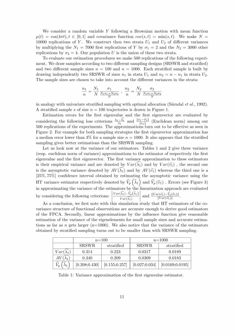
We consider a random variable Y following a Brownian motion with mean functionµ(t) = cos(4πt), t ∈ [0, 1] and covariance function cov(s, t) = min(s, t). We make N =10000 replications of Y . We construct then two strata U1 and U2 of different variancesby multiplying the N1 = 7000 first replications of Y by σ1 = 2 and the N2 = 3000 otherreplications by σ2 = 4. Our population U is the union of these two strata.

To evaluate our estimation procedures we make 500 replications of the following experi-ment. We draw samples according to two different sampling designs (SRSWR and stratified)and two different sample sizes n = 100 and n = 1000. Each stratified sample is built bydrawing independently two SRSWR of sizes n1 in stata U1 and n2 = n − n1 in strata U2.The sample sizes are chosen to take into account the different variances in the strata:

n1

n=N1

N

σ1

N1σ1+N2σ2N

,n2

n=N2

N

σ2

N1σ1+N2σ2N

in analogy with univariate stratified sampling with optimal allocation (Sarndal et al., 1992).A stratified sample s of size n = 100 trajectories is drawn in Figure 1.

Estimation errors for the first eigenvalue and the first eigenvector are evaluated byconsidering the following loss criterions λ1−cλ1

λ1and ‖v1− bv1‖

‖v1‖ (Euclidean norm) among our500 replications of the experiments. The approximations turn out to be effective as seen inFigure 2. For example for both sampling strategies the first eigenvector approximation hasa median error lower than 3% for a sample size n = 1000. It also appears that the stratifiedsampling gives better estimations than the SRSWR sampling.

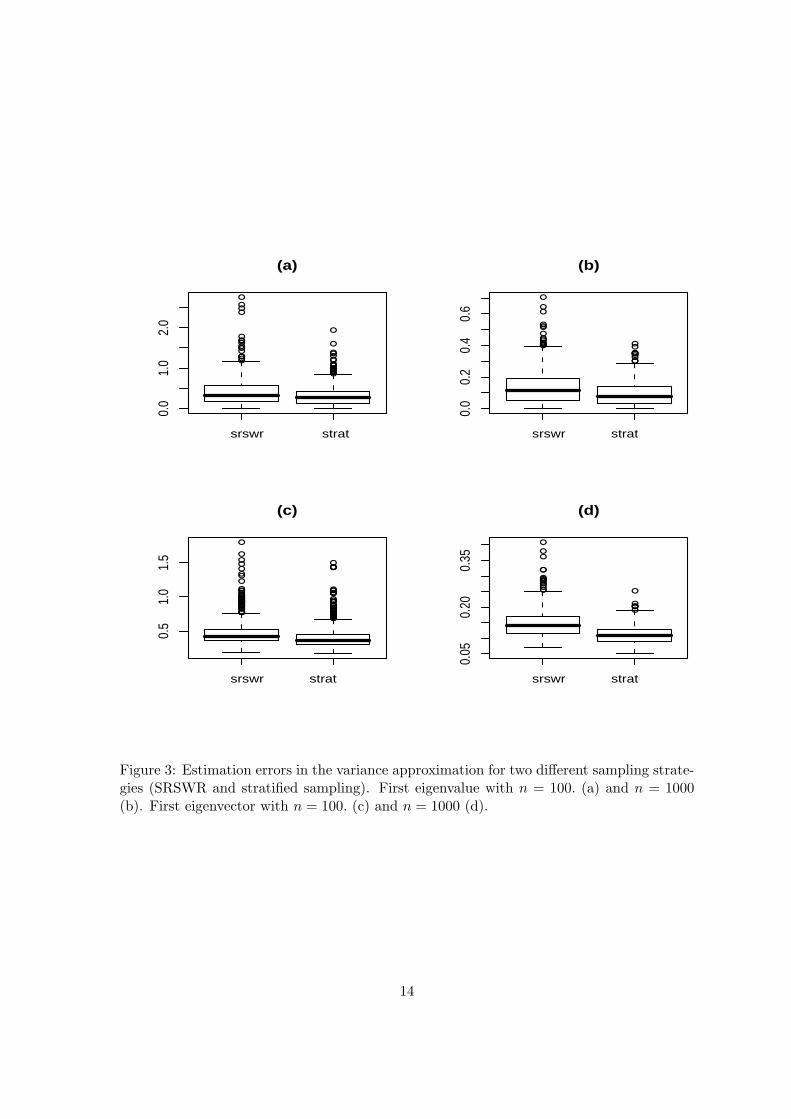
Let us look now at the variance of our estimators. Tables 1 and 2 give three variance(resp. euclidean norm of variance) approximations to the estimator of respectively the firsteigenvalue and the first eigenvector. The first variance approximation to these estimatorsis their empirical variance and are denoted by V ar(λ1) and by V ar(v1) , the second oneis the asymptotic variance denoted by AV (λ1) and by AV (v1) whereas the third one is a[25%, 75%] confidence interval obtained by estimating the asymptotic variance using theHT variance estimator respectively denoted by Vp

(λ1

)and Vp (v1) . Errors (see Figure 3)

in approximating the variance of the estimators by the linearization approach are evaluated

by considering the following criterions:∣∣∣∣V ar(cλ1)−bVp(bλ1)

V ar(cλ1)

∣∣∣∣ and ‖V ar( bv1)−bVp(bv1)‖‖V ar( bv1)‖ .

As a conclusion, we first note with this simulation study that HT estimators of the co-variance structure of functional observations are accurate enough to derive good estimatorsof the FPCA. Secondly, linear approximations by the influence function give reasonableestimation of the variance of the eigenelements for small sample sizes and accurate estima-tions as far as n gets larger (n=1000). We also notice that the variance of the estimatorsobtained by stratified sampling turns out to be smaller than with SRSWR sampling.

n=100 n=1000SRSWR stratified SRSWR stratified

V ar(λ1) 0.314 0.223 0.0317 0.0189AV (λ1) 0.340 0.209 0.0309 0.0183

Vp

(λ1

)[0.208;0.430] [0.155;0.257] [0.027;0.034] [0.0169;0.0195]

Table 1: Variance approximation of the first eigenvalue estimator.

11

0.0 0.2 0.4 0.6 0.8 1.0

−10

−50

510

t

Y

Figure 1: A stratified sample of n = 100 curves

n=100 n=1000SRSWR stratified SRSWR stratified

‖V ar(v1)‖ 0.450 0.286 0.0396 0.0265‖AV (v1)‖ 0.3997 0.287 0.0386 0.0267‖Vp (v1) ‖ [0.335;0.491] [0.252;0.354] [0.0371;0.0410] [0.0256;0.0280]

Table 2: Norm of the variance approximation of the first eigenvector estimator.

12

●

●●

●●

●

●●

●●

●

●

●

srswr strat

−0.4

0.0

0.4

(a)

●●

●

●

●

●●

●

●●

●

srswr strat

−0.1

0.1

0.2

(b)

●

●

●●

●

●

●

●

●●●

●

●

●

●●●●

●●●●●

●

●●●●●●

●

●●●●

srswr strat

0.05

0.15

0.25

(c)

●

●

●

●

●

●

●

●

●●●

srswr strat

0.01

0.03

0.05

(d)

Figure 2: Estimation errors for two different sampling strategies (SRSWR and stratifiedsampling). First eigenvalue with n = 100. (a) and n = 1000 (b). First eigenvector withn = 100. (c) and n = 1000 (d).

13

●

●

●

●

●●

●

●●

●●

●

●

●

●

●

●

●

●●●●

●●

●●●●●

●

●●

●

●

●

●

srswr strat

0.0

1.0

2.0

(a)

●

●

●

●●●

●

●

●

●

●

●

●●●

●●●●●

●

●

●●●

srswr strat

0.0

0.2

0.4

0.6

(b)

●

●

●

●●

●

●

●

●

●

●●●

●

●●

●

●

●●●

●●

●

●

●

●

●

●●

●

●

●●●

●

●

●

●

●

●●●

●

●

●

●●

●●

●●

●

●●

●

●●

●

●●●●

●

●

●●

●

●

●●

●

●

●●●

●●

●

●

●

srswr strat

0.5

1.0

1.5

(c)

●

●●

●

●

●

●●●●●

●

●

●●

●

●

●

●●●●

srswr strat

0.05

0.20

0.35

(d)

Figure 3: Estimation errors in the variance approximation for two different sampling strate-gies (SRSWR and stratified sampling). First eigenvalue with n = 100. (a) and n = 1000(b). First eigenvector with n = 100. (c) and n = 1000 (d).

14

Appendix : proofs

Proof of proposition 3.1.Let us introduce αk = Ik

πk− 1, we have

N −NN

=1N

∑k∈U

αk.

Noting that with assumptions (A2) and (A3), E(α2k) = (1−πk)/πk < (1−πk)/λ, |E(αkα`)| =

|∆k`/(πkπ`)| ≤ |∆k`|/λ2, and taking now the expectation, according to the sampling distri-bution p, we get

Ep

(N −NN

)2

=1N2

∑k,`∈U

Ep(α`αk)

=1N2

∑k∈U

1− πkπk

+∑k∈U

∑`6=k

∆k`

πkπ`

≤ 1

N2

(N

λ+N(N − 1)

n

nmax |∆k`|λ2

)= O

(1n

)(14)

which is the first result. Looking now at the estimator of the mean function, we have

µ− µ =1N

∑k∈U

αkYk +(

1

N− 1N

)∑k∈s

1πkYk

=1N

∑k∈U

αkYk +

(N − NN

)µ

By assumptions (A1)-(A3) it is clear that ‖µ‖ = O(1) and consequently Ep

∥∥∥N− bNN µ

∥∥∥2=

O(n−1). The first term of the right side of the inequality is dealt with as in (14), noticingthat ‖Yk‖ ≤ C for all k:

Ep

∥∥∥∥∥ 1N

∑k∈U

αkYk

∥∥∥∥∥2

=1N2

∑k,`∈U

Ep (α`αk) 〈Yk, Y`〉

≤ 1N2

∑k,`∈U

|Ep(α`αk)| ‖Yk‖ ‖Y`‖

= O

(1n

).

To complete the proof, let us introduce the operator Zk = Yk ⊗ Yk and remark that

Γ− Γ =1N

∑k∈U

αkZk +(

1

N− 1N

)∑k∈s

1πkZk + µ⊗ µ− µ⊗ µ

15

By assumption (A1), we have that |〈Zk, Z`〉2| ≤ ‖Yk‖2 ‖Y`‖2 ≤ C4, for all k and ` and weget with similar arguments as above that

Ep

∥∥∥∥∥ 1N

∑k∈U

αkZk

∥∥∥∥∥2

2

= O

(1n

)

and Ep

∥∥∥( 1bN − 1N

)∑k∈s

1πkZk

∥∥∥2

2= O(n−1). Remarking now that

‖µ⊗ µ− µ⊗ µ‖2 ≤ ‖(µ− µ)⊗ µ‖2 + ‖µ⊗ (µ− µ)‖2

the result is proved.Consistency of the eigenelements is an immediate consequence of classical properties of

the eigenelements of covariance operators. The eigenvalues (see e.g. Dauxois et al., 1982)satisfy

|λj − λj | ≤∥∥∥Γ− Γ

∥∥∥2.

On the other hand, Lemma 4.3 by Bosq (2000) tells us that

‖vj − vj‖ ≤ Cδj

∥∥∥Γ− Γ∥∥∥

2

where δ1 = 2√

2(λ1 − λ2)−1 and for j ≥ 2,

δj = 2√

2 max[(λj−1 − λj)−1, (λj − λj+1)−1

]. (15)

This concludes the proof. 2

Before giving the proof of proposition 3.2 let us state the following LemmaLemma: Consider the functional T =

PU Yk

N . Then T (M) = T(MN

)and IT

(MN , Yk

)=

N · IT (M,Yk).Proof :

IT

(M

N,Yk

)= lim

h→0

T (M + hNδYk)− T (M)

h= lim

h→0

1h

[∫Yd(M + hNδYk

)∫d(M + hNδYk

)−∫Yd(M)∫d(M)

]= lim

h→0

1h+ 1

(yk −

tYN

)= yk −

tYN

= N · IT (M,Yk)

2

Proof of proposition 3.2Considering first the mean curve µ, we get directly

µ(M + εδy) =1

N + ε

(∑`∈U

Y` + εy

)= µ+

ε

N(y − µ) + o(ε),

so that

Iµ(M,Yk) =1N

(Yk − µ).

Let us first note that perturbation theory (Kato, 1966, Chatelin 1983) allows us to get theinfluence function of the eigenelements provided the influence function of the covariance

16

operator is known. Indeed, let us consider the following expansion of Γ according to someoperator Γ1,

Γ(ε) = Γ + εΓ1 + o(ε), (16)

we get from perturbation theory that the eigenvalues satisfy

λj(ε) = λj + ε tr (Γ1Pj) + o(ε), (17)

where Pj = vj ⊗ vj is the projection onto the space spanned by vj and the trace of anoperator ∆ defined on L2[0, 1] is defined by tr(∆) =

∑j〈∆ej , ej〉 for any basis ej , j ≥ 1 of

L2[0, 1].There exists a similar result for the eigenfunctions which states, provided ε is smallenough and for simplicity that the non null eigenvalues are distinct, that

vj(ε) = vj + ε (SjΓ1(vj)) + o(ε), (18)

where operator Sj is defined on L2[0, 1] as follows

Sj =∑`6=j

v` ⊗ v`λj − λ`

.

So going back to the notion of influence function, if we get an expression for Γ1 in ourcase, we will be able to derive the influence function for the eigenelements. The influencefunction of Γ can be computed directly using the definition,

Γ(ε) = Γ(M + εδy)

=1

N + ε

(∑`∈U

(Y` ⊗ Y`) + ε(y ⊗ y)

)− 1

(N + ε)2(Nµ+ εy)⊗ (Nµ+ εy)

= Γ +ε

N(y ⊗ y − µ⊗ µ− Γ)− ε

N(µ⊗ (y − µ) + (y − µ)⊗ µ) + o(ε)

= Γ +ε

N((y − µ)⊗ (y − µ)− Γ) + o(ε) (19)

so that

IΓ(M,Yk) =1N

((Yk − µ)⊗ (Yk − µ)− Γ) .

The combination of (17) and (19) give us the influence function of the jth eigenvalue

Iλj(M,Yk) =1N

(〈Yk − µ, vj〉2 − λj

)as well as the influence function of the jth eigenfunction (since 〈vj , v`〉 = 0 when j 6= `)

Ivj(M,Yk) =1N

∑6=j

〈Yk − µ, vj〉〈Yk − µ, v`〉λj − λ`

v`

and the first part of proposition is proved. Now, we have immediately with Lemma abovethat IT

(MN , Yk

)= NIT (M,Yk) for T equal to µ or Γ. As for λj , we use (17) with

Γ1 = IΓ(MN , Yk

)= NIΓ(M,Yk) which implies that Iλj

(MN , Yk

)= NIλj(M,Yk). We

prove in the same way for vj using (18). 2

17

Proof of proposition 3.3Let us begin with the mean function, we have that Iµ

(MN , Y

)= NIµ(M,Y ) and using (8)

for α = 0, the remainder term is defined as follows

Rµ

(M

N,M

N

)= µ− µ−

∫Iµ(M,Y )d(M −M)

andRµ

(cMN ,

MN

)= µ− µ− 1

N

∑k∈s

Yk − µπk

= µ(

1− bNN

)+ µ

( bNN − 1

)= (µ− µ)

( bNN − 1

)= op(n−1/2),

since µ− µ = OP (n−1/2) and (N −N)/N = OP (n−1/2) by proposition 3.1.For the covariance operator, we have

RΓ

(M

N,M

N

)= Γ− Γ− 1

N

∑k∈s

1πk

((Yk − µ)⊗ (Yk − µ)− Γ)

= Γ

(N

N− 1

)+ Γ− 1

N

∑k∈s

1πk

(Yk − µ)⊗ (Yk − µ)

=(

Γ− Γ)(N

N− 1

)− N

N((µ− µ)⊗ (µ− µ))

= op(n−1/2), (20)

noticing that1N

∑k∈s

Yk ⊗ Ykπk

=N

N

(Γ + µ⊗ µ

).

To study the remainder terms for the eigenelements, we need to go back to the pertur-bation theory and equations (16), (17) and (18). According to (20), with ε = n−1/2, we canwrite

Γ1 =√n

(1N

∑k∈s

1πk

((Yk − µ)⊗ (Yk − µ)− Γ) +RΓ

(M

N,M

N

)). (21)

Introducing now (21) in equation (17), we get noting that 〈RΓ

(cMN ,

MN

)vj , vj〉 = op(n−1/2),

λj − λj =1N

∑k∈s

1πk

(〈Yk − µ, vj〉2 − 〈Γvj , vj〉

)+ op(n−1/2)

=∫Iλj(M,Y )d(M −M) + op(n−1/2)

which proves that Rλj

(cMN ,

MN

)= op(n−1/2). Using now (18) and since SjRΓ

(cMN ,

MN

)vj =

op(n−1/2), we can check with similar arguments that

vj − vj = Sj

(1N

∑k∈s

1πk

(〈Yk − µ, vj〉(Yk − µ)− λjvj)

)+ op(n−1/2)

18

=1N

∑k∈s

1πk

∑6=j

〈Yk − µ, vj〉〈Yk − µ, v`〉λj − λ`

v` + op(n−1/2)

=∫Ivj(M,Y )d(M −M) + op(n−1/2)

and the proof is complete. 2

Proof of proposition 3.4.

We prove the result for functional linearized variables uk. For real valued linearizedvariables, for instance for an eigenvalue λj , the proof is similar replacing the tensor productwith usual product and the norm || · ||2 with the absolue value | · |. Let us denote by

AV (T (M)) =∑s

∑s

∆kl

πkl

ukπk⊗ ulπl

=∑U

∑U

∆kl

πkl

ukπk⊗ ulπlIkIl

and by

A =∥∥∥AV (T (M))− AV (T (M))

∥∥∥2

and B =∥∥∥AV (T (M))− Vp(T (M))

∥∥∥2.

It is clear that∥∥∥AV (T (M))− Vp(T (M))∥∥∥

2≤ A+B.

Let us consider

Ep(A2)

=∑k,l∈U

∑k′,l′∈U

Ep

(1− IkIl

πkl

)(1− Ik′Il′

πk′l′

)⟨ukπk⊗ ulπl,uk′

πk′⊗ ul′

πl′

⟩2

. (22)

Using the fact that ‖uk ⊗ ul‖2 ≤ ‖uk‖‖ul‖ and since it is easy to check that ‖uk‖ < CN−1

where C is a constant that does not depends on k, we get, under assumptions (A2), (A3)and (A4), with a similar decomposition as in Breidt and Opsomer (2000, proof of Th. 3)that Ep

(A2)

= o(n−2) and thus Ep(A) = o(n−1).Let us study now the second term B and examine separately the case of the mean

function and the eigenvalues and the case of the eigenfunctions which can not be dealt withthe same way. We can prove, under assumptions (A2) and (A3), with similar manipulationsas before that there exist some positive constant C2, C3, C4 and C5 such that

Ep (B) = Ep

∥∥∥∥∥∑k∈U

∑l∈U

∆kl

πklIkIl

(ukπk⊗ ulπl− ukπk⊗ ulπl

)∥∥∥∥∥2

≤∑k∈U

∑l∈U

Ep

∣∣∣∣∆kl

πkl

∣∣∣∣ IkIl ∥∥∥∥ukπk ⊗ ulπl− ukπk⊗ ulπl

∥∥∥∥2

≤∑k∈U

∑l∈U

(Ep

(∆kl

πklIkIl

)2)1/2(

Ep

∥∥∥∥ukπk ⊗ ulπl− ukπk⊗ ulπl

∥∥∥∥2

2

)1/2

≤ C2

N

∑k∈U

∑l 6=k

(Ep

(‖(uk − uk)⊗ ul − uk ⊗ (ul − ul)‖22

))1/2

+C3

∑k∈U

(Ep

(‖(uk − uk)⊗ uk − uk ⊗ (uk − uk)‖22

))1/2

19

≤ C4

N

∑k∈U

∑l 6=k

(Ep ‖uk − uk‖2 ‖ul‖2 + Ep ‖ul − ul‖2 ‖uk‖2

)1/2

+C5

∑k∈U

(Ep

(‖uk − uk‖2 (‖uk‖2 + ‖uk‖2

))1/2

For k 6= l we have with assumption (A3) that ∆2kl ≤ CN−2. Furthermore, since n ≤

N ≤ n/λ, the estimated linearized variables for the mean function satisfy ‖uk‖2 = O(n−2)uniformly in k as well as for the eigenvalues (uk)2 = O(n−2).

For the mean function µ we have

uk − uk =1N

(µ− µ) +1

N

N −NN

(Yk − µ)

and thus we easily get that Ep‖uk − uk‖2 = O(N−3) uniformly in k. Considering theeigenvalues, we have

uk − uk =1N

(〈Yk − µ, vj〉2 − 〈Yk − µ, vj〉2 + λj − λj)−1

N

N −NN

(〈Yk − µ, vj〉2 − λj).

After some manipulations we also get that Ep(uk − uk)2 = O(N−3) uniformly in k. Com-bining the previous results we get Ep(B) = o(n−1) and the result is proved.

The technique is different for the eigenfunctions v1, . . . , vq because we can not boundeasily terms like Ep(λj− λj+1)−1 which appear in the estimators of the linearized variables.By Cauchy Schwartz inequality we have

B ≤

∑k∈U

∑l 6=k

(∆klIkIlπklπkπl

)21/2∑

k∈U

∑l 6=‖uk ⊗ ul − uk ⊗ ul‖22

1/2

(23)

+

(∑k∈U

(∆klIkπklπ

2k

)2)1/2(∑

k∈U‖uk ⊗ uk − uk ⊗ uk‖22

)1/2

(24)

By assumptions (A2) and (A3) we have, for k 6= l

Ep

(∆klIkIlπklπkπl

)2

=∆2kl

πklπ2kπ

2l

≤ C6

n2,

for some constant C6 that does not depend on k and l. When k = l, we have Ep(

∆kkIkπ3

k

)2≤

C7. Thus, by Markov inequality we have∑k∈U

∑l 6=k

(∆klIkIlπklπkπl

)21/2

= Op(1),

and (∑k∈U

(∆kkIkπ3k

)2)1/2

= Op(√n).

20

Considering the terms containing linearized variables in (23) and (24), we have thegeneral inequality∑

k∈U

∑l 6=k‖uk ⊗ ul − uk ⊗ ul‖22 ≤ 2

∑k∈U

∑l 6=k‖uk − uk‖2 ‖ul‖2 + ‖ul − ul‖2 ‖uk‖2 .

Let us make now the following decomposition

‖uk − uk‖ ≤ ‖Nuk‖

(N −NNN

)+

1

N

∥∥∥N uk −Nuk∥∥∥ (25)

with

Nuk − N uk = 〈Yk − µ, vj〉∑` 6=j

〈Yk − µ, v`〉λj − λ`

v` − 〈Yk − µ, vj〉∑`6=j

〈Yk − µ, v`〉λj − λ`

v`.

It is clear that ‖Nuk‖ = O(1) uniformly in k and( bN−NN bN

)= Op(n−3/2). We have for the

second right hand term of inequality (25),

∥∥∥Nuk − N uk∥∥∥ ≤ |〈Yk − µ, vj〉 − 〈Yk − µ, vj〉|

∥∥∥∥∥∥∑`6=j

〈Yk − µ, v`〉λj − λ`

v`

∥∥∥∥∥∥ (26)

+ |〈Yk − µ, vj〉|

∥∥∥∥∥∥∑` 6=j

〈Yk − µ, v`〉λj − λ`

v` −∑`6=j

〈Yk − µ, v`〉λj − λ`

v`

∥∥∥∥∥∥ (27)

It is clear that the first term at the right hand side of previous inequality satisfies, uniformlyin k,

Ep

|〈Yk − µ, vj〉 − 〈Yk − µ, vj〉|∥∥∥∥∥∥∑`6=j

〈Yk − µ, v`〉λj − λ`

v`

∥∥∥∥∥∥2

= O

(1n

).

Let us introduce the random variable

T = min(λj − λj+1, λj−1 − λj) min(λj − λj+1, λj−1 − λj),

the eigenvalues being distinct, we have with Proposition 1 that

1T

= Op(1).

As far as the second term in (27) is concerned we can write∥∥∥∥∥∥∑` 6=j

(λj − λ`)〈Yk − µ, v`〉v` − (λj − λ`)〈Yk − µ, v`〉v`(λj − λ`)(λj − λ`)

∥∥∥∥∥∥2

(28)

≤4∣∣∣λj − λj∣∣∣2T 2

∑6=j〈Yk − µ, v`〉2 +

4T 2

∑`6=j

(λ` − λ`)2〈Yk − µ, v`〉2

+4λ2j

∥∥∥∥∥∥∑6=j

〈Yk − µ, v`〉v` − 〈Yk − µ, v`〉v`(λj − λ`)(λj − λ`)

∥∥∥∥∥∥2

. (29)

21

We have seen that sup` |λ` − λ`|2 ≤∥∥∥Γ− Γ

∥∥∥2and thus the first two terms in (29) are

Op(n−1).The assumption that Γ is a finite rank operator is needed to deal with the last term of

(29). Using the fact that ‖v` − v`‖ ≤ Cδj

∥∥∥Γ− Γ∥∥∥ where δj is defined in (15), we also get

that this last term is also Op(n−1).Combining all these results we finally get that, uniformly in k

‖uk − uk‖ = Op(n−3/2)

It can be checked easily, under the finite rank assumption of Γ that, uniformly in k,‖uk‖ = Op(n−1) and ‖uk‖ = O(n−1). Going back now to (23) and (24) we get thatB = Op(1)Op(n−3/2) +Op(n1/2)Op(n−2) = op(n−1). This concludes the proof.

2

Acknowledgments. We would like to thank Andre Mas for helpful comments.

References

Berger, Y.G, Skinner, C.J (2005). A jacknife variance estimator for unequal probabilitysampling. J. R. Statist. Soc B, 67, 79-89.

Besse, P.C and Ramsay, J.O. (1986). Principal component analysis of sampled curves.Psychometrika, 51, 285-311.

Besse, P.C., Cardot, H. and Stephenson, D.B. (2000). Autoregressive Forecasting of SomeFunctional Climatic Variations. Scand. J. Statist., 27, 673-687.

Bosq, D. (2000). Linear Processes in Function Spaces. Lecture Notes in Statistics, 149,Springer.

Breidt, F.J. and Opsomer, J.D. (2000). Local Polynomial Survey Regression Estimatorsin Survey Sampling. The Annals of Statistics, 4, 1026-1053.

Campbell, C. and Little, A. D. (1980). A Different View of Finite Population Estima-tion. Proceeding of the Section on Survey Research Methods, American StatisticalAssociation. 319-324.

Cardot, H. (2000). Nonparametric estimation of the smoothed principal componentsanalysis of sampled noisy functions. J. Nonparametr. Stat., 12, 503-538.

Cardot, H., Faivre, R. and Goulard, M. (2003). Functional approaches for predictingland use with the temporal evolution of coarse resolution remote sensing data. J. ofApplied Statistics, 30, 1185-1199.

Castro, P., Lawton, W. and Sylvestre, E. (1986). Principal Modes of Variation for Pro-cesses with Continuous Sample Curves. Technometrics, 28, 329-337.

Chatelin, F. (1983). Spectral approximation of linear operators. Academic Press, NewYork

22

Chiky, R., Hebrail, G. (2007). Generic tool for summarizing distributed data streams.Preprint.

Chiou, J.M., Muller, H.G., Wang, J.L., Carey, J.R. (2003). A functional multiplicativeeffects model for longitudinal data, with application to reproductive histories of femalemedflies. Statist. Sinica 13, 1119-1133.

Croux, C., Ruiz-Gazen, A. (2005). High breakdown estimators for principal components :the projection-pursuit approach revisited. J. Multivariate Analysis, 95, 206-226.

Cuevas, A., Febrero, M. and Fraiman, R. (2002). Linear functional regression: The caseof fixed design and functional response. Canadian Journal of Statistics, 30, 285-300.

Dauxois, J., Pousse, A., and Romain, Y. (1982). Asymptotic theory for the principalcomponent analysis of a random vector function: some applications to statisticalinference. J. Multivariate Anal., 12, 136-154.

Dessertaine A. (2006). Sondage et series temporelles: une application pour la previsionde la consommation electrique. 38emes Journees de Statistique, Clamart, Juin 2006.

Deville, J.C. (1974). Methodes statistiques et numeriques de l’analyse harmonique. Ann.Insee, 15, 3-104.

Deville, J.C. (1999). Variance estimation for complex statistics and estimators: lineariza-tion and residual techniques. Survey Methodology, 25, 193-203.

Ferraty, F. and Vieu, P. (2006). Nonparametric Functional Data Analysis, Theory andApplications. Springer Series in Statistics, Springer, New-York.

Hampel, F. R. (1974). The influence curve and its role in robust statistics. J. Am. Statist.Ass., 69, 383-393.

Hastie, T. and Mallows, C. (1993). A discussion of “A statistical view of some chemomet-rics regression tools” by I.E. Frank and J.H. Friedman. Technometrics, 35, 140-143.

Isaki, C.T. and Fuller, W.A. (1982). Survey design under the regression superpopulationmodel. J. Am. Statist. Ass. 77, 89-96.

James, G., Hastie, T., and Sugar, C. (2000). Principal Component Models for SparseFunctional Data. Biometrika, 87 , 587-602.

Kato, T. (1966). Perturbation theory for linear operators. Springer Verlag, Berlin.

Kirkpatrick, M. and Heckman, N. (1989). A quantitative genetic model for growth, shape,reaction norms and other infinite dimensional characters. J. Math. Biol., 27, 429-450

Kneip, A. and Utikal, K.J. (2001). Inference for Density Families Using Functional Prin-cipal Component Analysis. J. Am. Statist. Ass., 96, 519-542.

Mises, R., v (1947). On the asymptotic distribution of differentiable statistical functions.Ann. Math. Statist., 18, 309-348.

Ramsay, J. O. and Silverman, B.W. (2002). Applied Functional Data Analysis: Methodsand Case Studies. Springer-Verlag.

23

Ramsay, J. O. and Silverman, B.W. (2005). Functional Data Analysis. Springer-Verlag,second edition.

Robinson, P.M. and Sarndal, C.E. (1983). Asymptotic properties of the generalized regres-sion estimator in probability sampling. Sankhya : The Indian Journal of Statistics,45, 240-248.

Serfling, R. (1980). Approximation Theorems of Mathematical Statistics, John Wiley andSons.

Silverman, B.W. (1996). Smoothed functional principal components analysis by choice ofnorm. Ann. Statist., 24, 1-24.

Skinner, C.J, Holmes, D.J, Smith, T.M.F (1986). The Effect of Sample Design on PrincipalComponents Analysis. J. Am. Statist. Ass. 81, 789-798.

24