Joint modeling of paired sparse functional data using

principal components

By LAN ZHOU

JIANHUA Z. HUANG and RAYMOND J. CARROL

Department of Statistics, Texas A&M University, College Station,

TX 77843, U.S.A.

lzhou@stat.tamu.edu

jianhua@stat.tamu.edu carroll@stat.tamu.edu

Summary

Studying the relationship between two paired longitudinally observed variables is an

important practical problem. We propose a modeling framework for this problem using

functional principal components. The data for each variable are viewed as smooth curves

measured at discrete time points plus random errors. While the curves for each variable are

summarized using a few important principal components, the association of the two longi-

tudinal variables is modeled through the association of the principal component scores. We

use penalized splines to model the mean curves and the principal component curves and cast

the proposed model into a mixed effects model framework for model fitting, prediction and

inference. The proposed method can be applied in the difficult case that the measurement

times are irregular and sparse and may differ widely across individuals.

Some key words: Functional data, Longitudinal data, Mixed effects models, Penalized

splines, Principal components, Reduced rank models.

1

1 Introduction

Understanding the relationship between two paired longitudinal observed variables is an

important practical problem. Regression models for longitudinal data have been studied

extensively and can be used for such a purpose (e.g., Liang & Zeger, 1986; Fahrmeir &

Tutz, 1994; Moyeed & Diggle, 1994; Zeger & Diggle, 1994; Lin & Ying, 2001). As an

extension of varying coefficient models (Hoover et al., 1998; Wu et al, 1998; Huang et al.,

2002), Liang et al. (2003) directly addressed this problem and proposed to model the paired

longitudinal variables using a mixed effects varying coefficient model with measurement error

in covariates. Let Xij and Yij denote longitudinal observations of a covariate and response

for subject i at time occasion tij. The model of Liang et al. can be written as

Yij = β0(tij) + γ0i(tij) +Xij{β1(tij) + γ1i(tij)}+ ei(tij), 1 ≤ j ≤ mi, 1 ≤ i ≤ n.

where β0(t) and β1(t) are fixed functions, γ0i(t) and γ1i(t) are mean zero subject-specific

random functions, and ei(t) are mean zero error processes. Different from many existing

work, the Liang et al. method effectively models the within-subject correlation in a flexible

way by considering subject-specific regression coefficient functions, and it also takes into

account measurement error in covariates.

However, the regression based methods including Liang et al. (2003) have several limita-

tions.

• One needs to distinguish response and regressor variables, but sometimes such distinc-

tion is not natural and switching the roles of regressor and response in a regression

yields results that may not be easy to interpret. This calls for a method that deals

with the two variables in a symmetric manner.

• As in Liang et al. (2003), the regression based methods usually focus on the contem-

poraneous relationship (that is, the relationship at the same time point) between two

variables. One could include lagged variables as regressors, but there are technical

difficulties in implementation of their method when the observation times for different

subjects differ, as often occurs in practice.

• In addition, results from a contemporaneous regression model may be hard to inter-

pret when we wish to consider all time points from the past, collectively. The usual

interpretation of regression slope as the average change in response associated with a

1

unit increase in the regressor is hardly satisfactory since the regressors from different

time points are correlated.

To overcome these shortcomings, we propose an alternative approach to modeling asso-

ciation of paired longitudinal variables. The data for each variable are viewed as smooth

curves sampled at discrete time points plus random errors. The curves are decomposed as

the sum of a mean curve and subject specific deviations from the mean curve. The devia-

tions are subsequently summarized by scores on a few important principal component curves

extracted from the data. The association of the pair of curves is then modeled through as-

sociation of two low-dimensional vectors of principal component scores corresponding to the

two underlying variables. By modeling the mean curves and the principal component curves

as penalized splines, we cast our modeling approach into a mixed effects model framework

for model fitting, prediction and inference.

Since principal component curves summarize the important modes of variation in the

data, as in the usual application of principal component analysis, model interpretation is

enhanced, see Section 7 for an illustration using data. Use of a few significant principal

components helps reduce the difficult problem of modeling association of two paired curves

to the relatively easy task of modeling the association of two low-dimensional vectors. The

dimensionality reduction also improves statistical and numerical stability of the parameter

estimates.

Our method takes advantage of viewing longitudinal data as sparsely observed functional

data (Rice, 2004). Ramsay & Silverman (2005) provide a comprehensive treatment of func-

tional data analysis. The approach in this paper is most closely related to that of James et

al. (2000) and Rice & Wu (2001). However, those two papers considered only models for

single curves instead of paired curves as we do in this paper. Similar to James et al., our

approach is model-based where the principal component curves are direct output from the

fitted model. Yao et al. (2005a) proposed a different manner of principal components analy-

sis for sparse functional data through eigen decomposition of the covariance kernel estimated

using two-dimension smoothing. Yao et al. (2005b) dealt with the functional linear model for

longitudinal data using regression through principal component scores. Another approach

to modeling association of paired curves is functional canonical correlation (Leurgans et al.,

1993; He et al., 2003) but its adaptation to sparse functional data remains an open problem.

The paper is organized as follows. Section 2 reviews some existing methods for functional

2

principal component analysis of single curve data and discusses an extension with penalized

splines. In Section 3 we present the proposed model for paired functional data. Section 4 de-

scribes a penalized likelihood method for parameter estimation and outlines a computational

procedure. Methods for specifying splines and choosing the penalty parameters, selecting

the number of principal component curves and producing confidence intervals are given in

Section 5. Sections 6 presents simulation results. Application to a data example from an

AIDS clinical trial is presented in Section 7. The appendix collects relevant technical details.

2 The Mixed Effects Model for Single Curves

We review in this section existing work on the mixed effects model of single curves using

fixed-knot splines (Shi et al., 1996; James et al., 2000; Rice & Wu, 2001). We also extend

the existing methods by introducing regularization through penalized likelihood in the spirit

of penalized splines (Eilers & Marx, 1996; Ruppert et al., 2003). Penalized splines provide

more flexible fit than fixed-knot splines and are useful for handling problems with small

sample size.

2.1 The Mixed Effects Model

Shi et al. (1996) and Rice & Wu (2001) suggest using a set of smooth basis functions, bl(t),

l = 1, . . . , q, such as B-splines, to represent the curves, where the spline coefficients are

assumed to be random to capture the individual or curve specific effects. Let Yi(t) be the

value of the ith curve at time t and write

Yi(t) = µ(t) + hi(t) + εi(t), (1)

where µ(t) is the mean curve, hi(t) represents the departure from the mean curve for subject

i, and εi(t) is random noise with mean zero and variance σ2. Let b(t) = {b1(t), . . . , bq(t)}T be

the vector of basis functions evaluated at time t. Denote by β an unknown but fixed vector

of spline coefficients, and let γi be a random vector of spline coefficients for each curve with

covariance matrix Γ. When modeling µ(t) and hi(t) with a linear combination of B-splines,

(1) has the following mixed effects model form:

Yi(t) = b(t)Tβ + b(t)Tγi + εi(t). (2)

3

In practice Yi(t) is only observed at a finite set of time points. Let Yi be the vector

consisting of the ni observed values, let Bi be the corresponding ni by q spline basis matrix

evaluated at these time points, and let εi be the corresponding random noise vector with

covariance matrix σ2I. The mixed effects model for the observed data is

Yi = Biβ +Biγi + εi. (3)

The Expectation-Maximization (EM) algorithm can be used to calculate the maximum like-

lihood estimates β and Γ (Laird & Ware, 1982). Given these estimates, the best linear

unbiased prediction of the random effects γi’s are

γi = (σ2Γ−1 +BTi Bi)

−1BTi (Yi −Biβ).

The mean curve µ(t) can then be estimated by µ(t) = b(t)Tβ and the subject specific curves

hi(t) can be predicted as hi(t) = b(t)Tγi.

2.2 The Reduced Rank Model

Since Γ involves q(q + 1)/2 different parameters, for a sparse data set its estimate can be

highly variable, and the large number of parameters may also make the EM algorithm fail

to converge to the global maximum. James et al. (2000) pointed out these problems with

the mixed effects model and proposed instead a reduced rank model, where the individual

departure from the mean is modeled by a small number of principal component curves. The

reduced rank model is

Yi(t) = µ(t) +k∑j=1

fj(t)αij + εi(t) = µ(t) + f(t)Tαi + εi(t), (4)

where µ(t) is the overall mean, fj is the jth principal component function (curve), f =

(f1, . . . , fk)T, and εi(t) is the random error. The principal components are subject to the

orthogonality constraint∫fjfl = δjl, with δjl being the Kronecker δ. The components of the

random vector αi give the relative weights of the principal component functions for the ith

individual and are called principal component scores. The αi’s and εi’s are independent and

are assumed to have mean zero. The αi’s are taken to have a common covariance matrix

and the εi’s are assumed temporally uncorrelated with a constant variance of σ2.

Similar to the mixed effects model (2), we represent µ and f using B-splines. Let b(t) =

{b1(t), . . . , bq(t)}T be a spline basis with dimension q. Let θµ and Θf be, respectively, a

4

q-dimensional vector and a q by k matrix of spline coefficients. Write µ(t) = b(t)Tθµ and

f(t)T = b(t)TΘf . The reduced rank model then takes the form

Yi(t) = b(t)Tθµ + b(t)TΘfαi + εi(t),

εi(t) ∼ (0, σ2ε ), αi ∼ (0, Dα), Dα diagonal,

(5)

subject to

ΘTf Θf = I,

∫b(t)b(t)T dt = I. (6)

The equations in (6) imply that∫f(t)f(t)T dt = ΘT

f

∫b(t)b(t)T dtΘf = I,

which are the usual orthogonality constraints on the principal component curves.

The requirement that the covariance matrix Dα of αi is diagonal is for identifiability

purposes. Without restrictions (6), neither Θf nor Dα can be identified: only the covariance

matrix of Θfαi, namely ΘfDαΘTf , can be identified. To identify Θf and Dα, note that

Θfαi = Θf αi, where Θf = ΘfC and αi = C−1αi for any invertible k by k matrix C.

Therefore, by requiring that Dα be diagonal and that the Θf have orthonormal columns,

reparameterization by linear transformation is prevented. The identifiability condition is

more precisely given in the following lemma, which follows from the uniqueness of eigen

decomposition of a covariance matrix.

Lemma 1. Assume ΘTf Θf = I and that the first nonzero element of each column of Θf is

positive. Let αi be ordered according to their variances in decreasing order. Suppose the

elements of αi have different variances, that is, var(αi1) > var(αi2) > · · · > var(αik). Then

the model specified by (5) and (6) is identifiable.

In Lemma 1, the first nonzero element of each column of Θf is used to determine the

sign at the population level. With finite samples, it is best to use the element of the largest

magnitude in each column of Θf to determine the sign, since this choice is least influenced

by finite sample random fluctuation.

The observed data usually consist of Yi(t) sampled at a finite number observation times.

For each individual i, let ti1, . . . , tini be the different time points at which measures are

available. Write

Yi = {Yi(ti1), . . . , Yi(tini)}T, Bi = {b(ti1), . . . , b(tini)}T.

5

The reduced rank model can then be written as

Yi = Biθµ +BiΘfαi + εi,

ΘTf Θf = I, εi ∼ (0, σ2I), αi ∼ (0, Dα).

(7)

The orthogonality constraints imposed on b(t) are achieved approximately by choosing b(t)

such that (L/g)BTB = I, where B = {b(t1), . . . , b(tg)}T is the basis matrix evaluated on a

fine grid of time points t1, . . . , tg and L is the length of the interval where we take these grid

points; see Appendix A.1 for implementation details. Since (7) is also a mixed effects model,

an EM algorithm can be used to estimate the parameters. By focusing on a small number

of leading principal components, the reduced rank model (7) employs a much smaller set of

parameters than (3), and thus more reliable parameter estimates can be obtained.

2.3 The Penalized Spline Reduced Rank Model

The reduced rank model of James et al. (2000) uses fixed knot splines to model the smooth

mean function and principal components. For many applications, especially when the sample

size is small, only a small number of knots can be used in order to fit the model to data.

An alternative, more flexible approach is to use a moderate number of knots and apply a

roughness penalty to regularize the fitted curves.

For the reduced rank model (4)-(7), we can use a moderate q, for example, q = 10–20,

and employ the method of penalized likelihood, where roughness penalties are introduced

to force the fitted functions µ(t) and f1(t), . . . , fk(t) to be smooth. We focus on roughness

penalties of the form of integrated squared second derivatives, though other forms are also

applicable. One approach is to use the following as a penalty

λµ

∫{µ′′(t)}2 dt+ λf1

∫{f ′′1 (t)}2 dt+ · · ·+ λfk

∫{f ′′k (t)}2 dt, (8)

where λµ, λf1, . . . , λfk, are tuning parameters. However, for simplicity, we shall restrict

λf1 = · · · = λfk = λf and employ a penalty that uses only two tuning parameters. In terms

of model (7), this simplified penalty can be written as

λµθµ

∫b′′(t)b′′(t)Tθµ dt+ λf

d∑j=1

θTfj

∫b′′(t)b′′(t)T dt θfj, (9)

where θfj is the jth column of Θf .

6

Assume that the αi’s and εi’s are normally distributed. Then

Yi ∼ N(Biθµ, σ2I +BiΘfDαΘT

fBTi ), i = 1, . . . , n,

and −2× log likelihood based on Yi’s, omitting an irrelevant constant, is

n∑i=1

log(|σ2I +BiΘfDαΘT

fBTi |)

+ (Yi −Biθµ)T(σ2I +BiΘfDαΘTfB

Ti )−1(Yi −Biθµ).

The method of penalized likelihood minimizes a criterion function that is the sum of the

−2× log likelihood and the penalty in (9). While direct optimization is complicated, it is

easier to treat the αi’s as missing data and employ the EM algorithm. A modification of

the algorithm by James et al. (2000) that takes into account the roughness penalty can be

applied. The details are not presented here. The algorithm can also be obtained easily as a

simplification of our algorithm for joint modeling of paired curves to be given in Section 3.

3 The Mixed Effects Model for Paired Curves

For data consisting of paired curves, an important problem of interest is modeling the as-

sociation of the two curves. We first model each curve using the reduced rank principal

components model as discussed in Section 2.2, and then model the association of curves by

jointly modeling the principal component scores. Roughness penalties are introduced as in

Section 2.3 to obtain smooth fits of the mean curve and principal components.

Let Yi(t) and Zi(t) denote the two measurements at time t for the ith individual. The

reduced rank model has the form

Yi(t) = µ(t) +kα∑j=1

fj(t)αij + εi(t) = µ(t) + f(t)Tαi + εi(t), (10)

Zi(t) = ν(t) +

kβ∑j=1

gj(t)βij + ξi(t) = ν(t) + g(t)Tβi + ξi(t), (11)

where µ(t) and ν(t) are the mean curves, f = (f1, f2, . . . , fkα)T and g = (g1, g2, . . . , gkβ)T are

vectors of principal components, εi(t) and ξi(t) are measurement errors. The αi’s, βi’s, εi’s

and ξi’s are assumed to have mean zero. The measurement errors εi(t) and ξi(t) are assumed

uncorrelated with constant variance σ2ε and σ2

ξ respectively. It is also assumed that αi’s,

εi’s and ξi’s are mutually independent, and βi’s, εi’s and ξi’s are mutually independent. The

7

principal components are subject to the orthogonality constraint∫fjfl = δjl and

∫gjgl = δjl,

with δkl being the Kronecker delta.

For identifiability, the principal component scores αij, j = 1, . . . , kα are independent

with strictly decreasing variances (see Lemma 1). Similarly, the principal component scores

βij, j = 1, · · · , kβ are also independent with strictly decreasing variances. Denote the diago-

nal covariance matrices of αi and βi as Dα and Dβ, respectively.

The relationship between Yi(t) and Zi(t) is assumed through the correlation between the

principal component scores αi and βi. Specifically, we assume that cov(αi, βi) = C. Then αi

and βi are modeled jointly as followsαiβi

∼

{0

0

,

Dα C

CT Dβ

}. (12)

This is equivalent to a regression model

βi = Λαi + ηi, (13)

where Λ = CTD−1α or C = DαΛT. It follows from (13) that the covariance matrix of ηi

is Ση = Dβ − ΛDαΛT. We find this regression formulation to be more convenient when

calculating the likelihood function.

Note that the roles of Y (t) and Z(t) and therefore the roles of αi and βi are symmetric

in our modeling framework. In the regression formulation (13), however, αi and βi do not

appear to play symmetric roles and interpretation of Λ does depend on what is used as the

regressor and what is used as the response. We point out however that this formulation only

serves as a computational device. If we switch the roles of αi and βi we still get the same

estimates of the original parameters (Dα, Dβ, C).

Denote R = D−1/2α CD

−1/2β as the matrix of correlation coefficients, which provides a

scale-free measure of the association between αi and βi. We shall call Dα, Dβ together with

σ2ε and σ2

ξ the variance parameters and call the entries of R the correlation parameters.

We represent µ, ν, f and g using a basis of spline functions of the same dimension q. Note

that the use of different dimensionality is not necessary here because of the flexibility intro-

duced by using roughness penalties. The basis, denoted as b(t), is chosen to be orthonormal,

that is, the components of b(t) = {b1(t), . . . , bq(t)}T satisfy∫bj(t)bl(t) dt = δjl. Let θµ and

θν be a q-dimensional vector of spline coefficients such that

µ(t) = b(t)Tθµ and ν(t) = b(t)Tθν . (14)

8

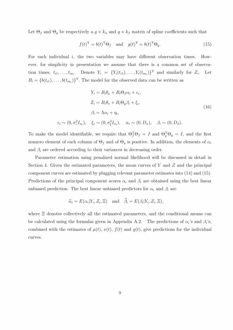
Let Θf and Θg be respectively a q × kα and q × kβ matrix of spline coefficients such that

f(t)T = b(t)TΘf and g(t)T = b(t)TΘg. (15)

For each individual i, the two variables may have different observation times. How-

ever, for simplicity in presentation we assume that there is a common set of observa-

tion times, ti1, . . . , tini . Denote Yi = {Yi(ti1), . . . , Yi(tini)}T and similarly for Zi. Let

Bi = {b(ti1), . . . , b(tini)}T. The model for the observed data can be written as

Yi = Biθµ +BiΘfαi + εi,

Zi = Biθν +BiΘgβi + ξi,

βi = Λαi + ηi,

εi ∼ (0, σ2ε Ini), ξi ∼ (0, σ2

ξIni), αi ∼ (0, Dα), βi ∼ (0, Dβ).

(16)

To make the model identifiable, we require that ΘTf Θf = I and ΘT

g Θg = I, and the first

nonzero element of each column of Θf and of Θg is positive. In addition, the elements of αi

and βi are ordered according to their variances in decreasing order.

Parameter estimation using penalized normal likelihood will be discussed in detail in

Section 4. Given the estimated parameters, the mean curves of Y and Z and the principal

component curves are estimated by plugging relevant parameter estimates into (14) and (15).

Predictions of the principal component scores αi and βi are obtained using the best linear

unbiased prediction. The best linear unbiased predictors for αi and βi are

αi = E(αi|Yi, Zi,Ξ) and βi = E(βi|Yi, Zi,Ξ),

where Ξ denotes collectively all the estimated parameters, and the conditional means can

be calculated using the formulas given in Appendix A.2. The predictions of αi’s and βi’s,

combined with the estimates of µ(t), ν(t), f(t) and g(t), give predictions for the individual

curves.

9

4 Fitting the Bivariate Reduced Rank Model

4.1 Penalized Likelihood

Assuming normality, the joint distribution of Yi and Zi is determined by the mean vector

and variance-covariance matrix, which are given by

E(Yi) = Biθµ, E(Zi) = Biθν ;

var(Yi) = BiΘfDαΘTfB

Ti + σ2

ε Ini , var(Zi) = BiΘgDβΘTgB

Ti + σ2

ξIni ;

cov(Yi, Zi) = BiΘfDαΛTΘTgB

Ti .

Let L(Yi, Zi) denote the contribution to the likelihood from subject i. The joint likelihood

for the whole data set is∏n

i=1 L(Yi, Zi). The method of penalized likelihood minimizes the

following criterion

− 2n∑i=1

log{L(Yi, Zi)}

+ λµθµ

∫b′′(t)b′′(t)T dt θµ + λf

k∑j=1

θTfj

∫b′′(t)b′′(t)T dt θfj

+ λνθν

∫b′′(t)b′′(t)T dt θν + λg

k∑j=1

θTgj

∫b′′(t)b′′(t)T dt θgj,

(17)

where dαj and dβj are, respectively, the jth diagonal element of Dα and Dβ, while θfj and

θgj are, respectively, the jth column of Θf and Θg. There are four regularization parameters,

which gives the flexibility of allowing different amounts of smoothing for mean curves and

principal components.

The likelihood is a complicated function of the parameters θµ, θν , Θf , Θg, Dα, Dβ, Λ,

σ2ε , σ

2ξ and thus it is difficult to minimize the criterion (17) directly. If the αi’s and βi’s were

observable, then the joint likelihood for (Yi, Zi, αi, βi) can be factored as

L(Yi, Zi, αi, βi) = f(Yi|αi)f(Zi|βi)f(βi|αi)f(αi).

Ignoring an irrelevant constant, it follows that the −2× log likelihood can be written as

10

follows:

−2log{L(Yi, Zi, αi, βi)}

= nilog(σ2ε ) +

1

σ2ε

(Yi −Biθµ −BiΘfαi)T(Yi −Biθµ −BiΘfαi)

+ nilog(σ2ξ ) +

1

σ2ξ

(Zi −Biθν −BiΘgβi)T(Zi −Biθν −BiΘgβi)

+ log(|Ση|) + (βi − Λαi)TΣ−1

η (βi − Λαi) + log(|Dα|) + αTi D−1α αi.

(18)

It is clear that the unknown parameters are separated in the log likelihood and therefore

separate optimization is feasible. We thus treat αi and βi as missing values and use the EM

algorithm (Dempster et al., 1977) to estimate the parameters. Given a set of current values

of the parameters, the EM algorithm updates the parameter estimates by minimizing the

conditional expectation of the penalized -2 × log likelihood, where the expectation is taken

under the distribution of parameters being set at their current values.

4.2 Conditional Distributions

The E-step of the EM algorithm consists of finding the prediction of the random effects

αi and βi and their moments based on (Yi, Zi) and the current parameter values. In this

section, all calculation is done given the current parameter values, although the dependence

in notation is suppressed throughout. The conditional distribution of (αi, βi) given (Yi, Zi)

is normal and is denoted asαiβi

∼ N

{µi,αµi,β

,Σi =

Σi,αα,Σi,αβ

Σi,βα,Σi,ββ

}. (19)

The desired predictions required by the EM algorithm are

αi = E(αi|Yi, Zi) = µi,α, βi = E(βi|Yi, Zi) = µi,β,

αiαTi = E(αiα

Ti |Yi, Zi) = αiα

Ti + Σi,αα, βiβT

i = E(βiβTi |Yi, Zi) = βiβ

Ti + Σi,ββ,

αiβTi = E(αiβ

Ti |Yi, Zi) = αiβ

Ti + Σi,αβ.

(20)

Calculation of the conditional moments of the multivariate normal distribution (19) is given

in Appendix A.2.

11

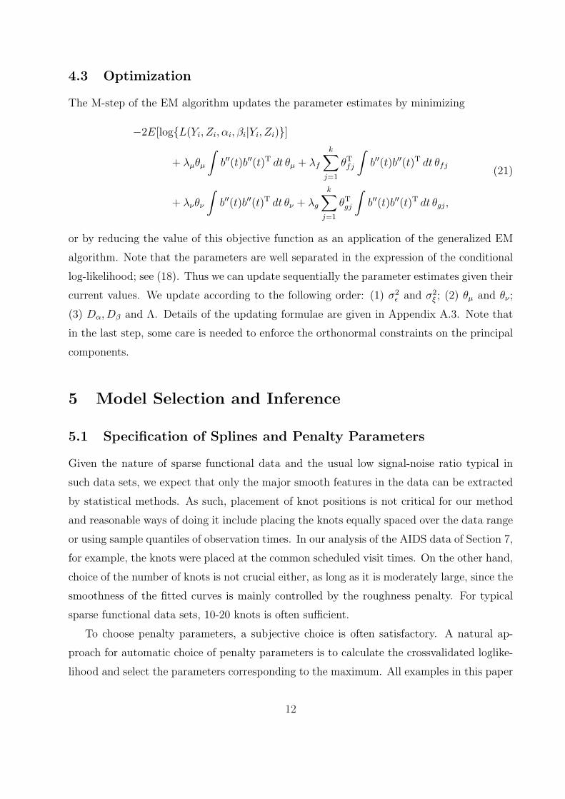
4.3 Optimization

The M-step of the EM algorithm updates the parameter estimates by minimizing

−2E[log{L(Yi, Zi, αi, βi|Yi, Zi)}]

+ λµθµ

∫b′′(t)b′′(t)T dt θµ + λf

k∑j=1

θTfj

∫b′′(t)b′′(t)T dt θfj

+ λνθν

∫b′′(t)b′′(t)T dt θν + λg

k∑j=1

θTgj

∫b′′(t)b′′(t)T dt θgj,

(21)

or by reducing the value of this objective function as an application of the generalized EM

algorithm. Note that the parameters are well separated in the expression of the conditional

log-likelihood; see (18). Thus we can update sequentially the parameter estimates given their

current values. We update according to the following order: (1) σ2ε and σ2

ξ ; (2) θµ and θν ;

(3) Dα, Dβ and Λ. Details of the updating formulae are given in Appendix A.3. Note that

in the last step, some care is needed to enforce the orthonormal constraints on the principal

components.

5 Model Selection and Inference

5.1 Specification of Splines and Penalty Parameters

Given the nature of sparse functional data and the usual low signal-noise ratio typical in

such data sets, we expect that only the major smooth features in the data can be extracted

by statistical methods. As such, placement of knot positions is not critical for our method

and reasonable ways of doing it include placing the knots equally spaced over the data range

or using sample quantiles of observation times. In our analysis of the AIDS data of Section 7,

for example, the knots were placed at the common scheduled visit times. On the other hand,

choice of the number of knots is not crucial either, as long as it is moderately large, since the

smoothness of the fitted curves is mainly controlled by the roughness penalty. For typical

sparse functional data sets, 10-20 knots is often sufficient.

To choose penalty parameters, a subjective choice is often satisfactory. A natural ap-

proach for automatic choice of penalty parameters is to calculate the crossvalidated loglike-

lihood and select the parameters corresponding to the maximum. All examples in this paper

12

use tenfold crossvalidation, which involves holding 10% of the subjects as a test set, fitting

the model to the remaining subjects, calculating the loglikelihood on the test set, and then

repeating the process nine more times. The criterion used for model selection is summation

of the ten calculated test set loglikelihoods.

There are four penalty parameters, so we need to search over a four dimensional space for

a good choice of these parameters. A multidimensional optimization algorithm such as the

downhill simplex method of Nelder and Mead (1965) can be used for our purpose. However

a crude grid search works well for all examples we considered. With five grid points on each

dimension, there are in total 625 possible combinations for four parameters. Implemented

in Fortran, this strategy is computationally feasible and has been used for the data example

in Section 7. One possible simplification is to let λµ = λν and λf = λg and thus reduce the

dimension to two. This simplification, with five grid points for each of the two dimensions,

has been used for our simulation study in Section 6.

5.2 Selection of the Number of Significant Principal Components

It is important to identify the number of important principal components in functional

principal component analysis. For the single curve model, choosing to fit too many principal

components can degrade the fit of them all (James, et al., 2000). Fitting too many principal

components in the joint modeling is even more harmful, since instability can result if we

try to estimate correlation coefficients among a set of latent random variables with large

differences in variances. In this section we propose a procedure for choosing the number of

important principal components.

First we apply the penalized spline reduced rank model in Section 2.3 to each variable

separately and use these single curve models to select the number of significant principal

components for each variable. We then fit the joint model using the chosen numbers of

significant principal components from fitting single curve models; the numbers are refined if

necessary. For the single curve models we use a stepwise addition approach. Specifically we

start with one principal component and then add one principal component at a time to the

model. The addition process stops if the variances of the scores of the principal components

already in the model do not change much after addition of one more principal component

and the variance of the scores of the newly added principal component is of much smaller

magnitude comparing with those already in the model.

13

A more detailed description of the procedure is as follows. Let ka and kb denote the

number of important principal components used in a single curve model for Y and for Z

respectively. Let D(k)α,l , 1 ≤ l ≤ k, denote the variances of the principal component scores for

an order-k model for Y . Similarly define D(k)β,l ’s for Z. The steps for choosing ka are:

• Start with k = 1 and increase k by one at a time until we decide to stop according to

the criterion described below.

• For each k, fit an order-k and order-(k+ 1) single curve model for Y . If D(k+1)α,l ' D

(k)α,l

for all 1 ≤ l ≤ k and D(k+1)α,k+1 < cD

(k+1)α,k for some pre-specified small constant c, stop at

k. The number of principal components to be modeled in the joint modeling is ka = k.

We select kb similarly. We have used c in the range from 1/25 to 1/9 in the above procedure.

The joint model is then fit with the selected ka and kb. The variances of the principal

component scores from fitting the joint model need not be the same as those from the single

curve models. A refinement using the joint model fit can be done via a stepwise deletion

procedure. If the variance of the scores of the last principal component is much smaller

than the variance of the scores of the previous principal component, delete that principal

component from the model. This can be done sequentially if necessary.

To check this procedure, we tested it on the simulated data sets from Section 6 where

in the true model, the variable Y has one significant principal component and the variable

Z has two significant principal components. The results of applying the procedure without

the second stage refinement are as follows. When c = 1/25 was used, among 200 simulation

runs, for variable Y , 97% picked 1 important principal component and 3% picked 2 important

principal components; for variable Z, 98% picked 2 important principal components and 2%

picked 3 important principal components. When c = 1/9 was used, in all simulations one

principal component was picked for variable Y ; for variable Z, in 99% of simulations two

principal components were picked and in 1% of simulations one principal component was

picked. The first stage stepwise addition process thus has already given a quite accurate

choice on the number of important principal components, and the second stage stepwise

deletion refinement is not necessary for this example. The use of the second stage refinement

will be illustrated using the data analysis in Section 7.

14

5.3 Confidence Intervals

The bootstrap can be applied to produce pointwise confidence intervals of the overall mean

functions for both variables and the principal components curves. It can also be used to

produce confidence intervals of the variance and correlation coefficient parameters. The

confidence intervals are formed using appropriate sample quantiles of relevant estimates

from the bootstrap samples. Here the bootstrap samples are obtained by resampling the

subjects, in order to preserve the correlation of observations within subject. When applying

the penalized likelihood to the bootstrap samples, the same specification of splines and

penalty parameters may be used.

6 Simulation

In this section we illustrate the performance of penalized likelihood in fitting the bivariate

reduced rank model using Monte Carlo simulation. In each simulation run, we have n = 50

subjects and each subject has up to 4 visits between time 0 and 100. We generated the

visit times by mimicking a typical clinical setting. The visit times for each subject were

generated sequentially where the spacings between the visits are normally distributed. The

actual generating procedure is as follows:

1. Each subject has a baseline visit, so ti1 = 0 for i = 1, . . . , 50.

2. For subject i, i = 1, . . . , 50, for k = 1, . . . , generate ti,k+1 such that ti,k+1 − ti,k ∼N(30, 102). Let ki be the first k such that k ≤ 4 and ti,k+1 > 100. The visit times for

subject i are ti,1, . . . , ti,ki .

At visit time t, subject i has two observations (Yit, Zit) where Yit and Zit are generated

according to

Yit = µ(t) + fy(t)αi + εit,

Zit = ν(t) + fz1(t)βi1 + fz2(t)βi2 + ξit.

Here the mean curves have the form µ(t) = 1 + t/100 + exp{−(t − 60)2/500} and

ν(t) = 1 − t/100 − exp{−(t − 30)2/500}. The principal component curves are fy(t) =

sin(2πt/100)/√

50, fz1(t) = fy(t) and fz2(t) = cos(2πt/100)/√

50. Notice that the princi-

pal component functions are normalized such that∫ 100

0f 2y (t) dt = 1,

∫ 100

0f 2z1(t) dt = 1 and

15

∫ 100

0f 2z2(t) dt = 1. Variable Z’s two principal component curves are orthogonal such that

∫ 100

0fz1(t)fz2(t) dt = 0. The principal component scores αi, βi1 and βi2 are independent

between subjects and their distributions are normal with mean 0 and variances Dα = 36,

Dβ1 = 36 and Dβ2 = 16 respectively. Variable Z’s two principal component scores, βi1 and

βi2, are independent. In addition, the correlation coefficient between αi and βi1 is ρ1 = −.8and that between αi and βi2 is ρ2 = −.45. The measurement errors εit and ξit are independent

and normally distributed with mean 0 and variance 0.5.

The penalized likelihood method was applied to fit the joint model with ka = 1 and

kb = 2. The number of important principal components was estimated using the procedure

given in Section 5.2. Penalty parameters were picked using tenfold crossvalidation on a grid

(λµ = λν in {k × 104} and λf = λg in {2k × 105} for k = 1, . . . , 5). Figure 1 shows fitted

mean curves and the principal component curves for five simulated data sets, along with

the true curves used in generating the data. Table 1 presents the sample mean and mean

squared error (MSE) of the variance and correlation parameters, based on 200 simulation

runs. Our joint modeling approach was compared with a separate modeling approach that

fits Y and Z separately using the single curve method described in Section 2.3. The single

curve method gives similar, but slightly worse (in terms of MSE), estimates of the variance

parameters. However, unlike the joint modeling approach, the single curve method does not

provide estimates of the correlation coefficients of the principal component scores. A naive

approach is to use the sample correlation coefficients of the best linear unbiased predictions

of the principal component scores from the single curve model. Since the best linear unbiased

predictions are shrinkage estimates, such calculated correlation coefficients can be seriously

biased, as shown in Table 1. Mean integrated squared errors (MISE) for estimating the mean

functions were also computed for the two approaches. The joint modeling approach reduced

the MISE compared to the separate modeling approach by 23% and 33% for estimating µ(·)and ν(·) respectively. It is not surprising that the joint modeling approach is more efficient

than separate modeling, as is well known in seemingly unrelated regressions (Zellner, 1962).

7 AIDS Study Example

In this section we illustrate our model and the proposed estimation method using a data

set from an AIDS clinical study conducted by the AIDS Clinical Trials Group, ACTG 315

16

(Lederman et al., 1998; Wu et al., 1999). In this study, forty-six HIV-1 infected patients were

treated with potent antiviral therapy consisting of ritonavir, 3TC and AZT. After initiation

of treatment at day 0, patients were followed for up to 10 visits. Scheduled visit times

common for all patients are 7, 14, 21, 28, 35, 42, 56, 70, 84 and 168 days. Since the patients

did not follow exactly the scheduled times and there were also missed visits for some patients,

the actual visit times are irregularly spaced and different for different patients. The visit

time varies from day 0 (first visit) to day 196. The purpose of our statistical analysis is to

understand the relationship between virologic and immunologic surrogate markers such as

plasma HIV RNA copies (viral load) and CD4+ cell counts during HIV/AIDS treatments.

In the notation of our joint model for paired functional data as detailed in Section 3,

denote Y for CD4+ cell counts divided by 100 and Z for the base 10 logarithm of plasma

HIV RNA copies. Following Liang et al. (2003), the viral load data below the limit of

quantification (100 copies per mL plasma) are imputed by the mid-value of the quantification

limit (50 copies per mL plasma). To model the curves on the time interval [0, 196], we

used cubic B-splines with 10 interior knots placed on scheduled visit days. The penalty

parameters were selected by tenfold crossvalidation. The resampling subject bootstrap was

used to obtain confidence intervals with the number of bootstrap repetitions being 1000.

Following the method described in Section 5.2, we took two steps to select the number of

important principle components. In the first step, the two variables were modeled separately

using the single curve method in Section 2.3. A sequence of models with different numbers of

principle component functions were considered and the corresponding variances of principal

component scores for these models are given in Table 2. We decided to use two principal

components for both Y and Z. In the second step, the model was fitted jointly with ka = 2

and kb = 2. The estimates of the variances are Dα1 = 110.1, Dα2 = 1.147, Dβ1 = 169.8 and

Dβ2 = 11.8. Given that the ratio between Dα2 and Dα1 is now about 1%, we decided to drop

the second principal component for CD4+ counts and use ka = 1 and kb = 2 in our final

model. Note that the ratio of Dβ2 and Dβ1 is about 7%, so for viral load, the second principal

component, even though included in the final model, is much less important compared with

the first principal component.

Figure 2 presents CD4+ cell counts and viral load over time, overlaid by their estimated

mean curves and 95% bootstrap pointwise confidence intervals for the means. It is seen from

these plots that on average, CD4+ cell counts increase while viral load decreases dramat-

17

ically until day 28. After CD4+ counts plateau out at 28 days, the viral load still drops

until about 50 days. The feature after 50 days in the viral load plot is an artifact of few

observations and an outlier affecting crossvalidation; the feature disappears with a larger

smoothing parameter.

In Figure 3 the estimated principal component curves of CD4+ counts and the viral load

are plotted, along with the corresponding 95% bootstrap pointwise confidence intervals. The

effect on the mean curves of adding and subtracting a multiple of each of the principal com-

ponent curves is also given in Figure 3, where the standard deviations of the corresponding

principal component scores are used as the multiplicative factors. The principal component

curve for the CD4+ counts is almost constant over the time range and corresponds to an

effect of a level shift from the overall mean curve. The first principal component curve for

the viral load corresponds to a level shift from the overall mean with the magnitude of the

shift increasing with time. The second principal component curve for the viral load changes

sign during the time course and corresponds to an opposite departure from the mean at the

beginning and the end of the time period. Compared with the first principal component, it

explains much less variability in the data and can be viewed as a correction factor to the

prediction made by the first principal component. Note that we did not know the shape of

the principal component curves prior to analysis, but it turns out that all estimated principal

component curves are rather smooth and close to a line. This may be due to the high level

of noise in the data that prevents identifying more subtle features; the data-driven crossval-

idation does not support use of smaller penalties. Given that the two principal components

are obtained from a high dimensional function space, dimension reduction is quite effective

in this example.

In Figure 4 we plot observed data for three typical subjects and corresponding mean

curves and best linear unbiased predictions of the underlying subject specific curves. The

predicted values of the scores corresponding to the first principal component of CD4+ counts

are 11.43, −7.15, −2.49 for the three subjects respectively. The predicted values of the scores

of the first principal component of viral load are 4.43, 5.11, 1.05, and those of the second

principal component are 4.26, 2.08, −1.50. These predicted scores and the graphs in Figure 4

agree with the interpretation of the principal components given in the previous paragraph.

For example, the first subject has a positive score while the second and third subjects

have a negative score on the first principal component of CD4+ counts, corresponding to a

18

downward and upward shift of the predicted curves from the mean curve, respectively. The

cross-over effect of the second principal component of viral load is clearly seen in the third

subject.

Estimates of variance and correlation parameters are given in Table 3 together with the

corresponding 95% bootstrap confidence intervals. Of particular interest is the parameter

ρ1, the correlation coefficient of αi1 and βi1, which are the scores corresponding to the

first principal component of CD4+ counts and viral load respectively. The estimated ρ1 is

statistically significantly negative, which suggests that a positive score on the first principal

component of CD4+ counts tends to be associated with a negative score on the first principal

component of viral load. In other words, for a subject with CD4+ count lower (or higher)

than the mean, the viral load tends to be higher (or lower) than the mean.

ACKNOWLEDGMENTS

Lan Zhou was supported by a postdoctoral training grant from the National Cancer Institute.

Jianhua Huang was partially supported by grants from the National Science Foundation

and the National Cancer Institute. Raymond J. Carroll was supported by grants from the

National Cancer Institute.

Appendix

A.1 Create a basis b(t) that satisfies the orthonormal constraints

Let b(t) = {b1(t), . . . , bq(t)}T be an initially chosen, not necessarily orthonormal, basis such

as the B-spline basis. There is a matrix of transformation T such that b(t) = TTb(t). This

T can be constructed as follows. Write B = {b(t1), . . . , b(tg)}T. Let B = QR be the QR

decomposition of B where Q has orthonormal columns and R is an upper triangular matrix.

Then T = (g/L)1/2R−T will be a desirable transformation matrix since

L

gBTB =

L

gTBTBTT =

L

gTRTQTQRTT = I.

19

A.2 The Conditional Moments of the Multivariate Normal Dis-

tribution (19)

Denote

Σ−1i =

Σαα

i ,Σαβi

Σβαi ,Σββ

i

.

Then the conditional distribution satisfies

f(αi, βi|Yi, Zi) ∝ exp

[−1

2{(αi − µi,α)T, (βi − µi,β)T}

Σαα

i ,Σαβi

Σβαi ,Σββ

i

αi − µi,αβi − µi,β

].

On the other hand, f(αi, βi|Yi, Zi) ∝ f(αi, βi, Yi, Zi). Comparing the coefficients of the

quadratic forms αTi Σαα

i αi, αTi Σαβ

i βi, and βTi Σββ

i βi in the two expressions of the conditional

distribution, we obtain

Σααi = D−1

α + ΛTΣ−1η Λ +

1

σ2ε

ΘTfB

Ti BiΘf ,

Σαβi = −ΛTΣ−1

η ,

Σββi = Σ−1

η +1

σ2ξ

ΘTgB

Ti BiΘg.

These can be used to calculate Σi,αα, Σi,αβ and Σi,ββ, by using the formulae

Σi,αα =(Σααi − Σαβ

i (Σββi )−1Σβα

i

)−1,

Σi,αβ = −Σi,ααΣαβi (Σββ

i )−1,

Σi,ββ =(Σββi − Σβα

i (Σααi )−1Σαβ

i

)−1,

or direct matrix inversion of Σ−1i .

Similarly, comparing the coefficients of the first order terms, we obtain

Σααi µi,α + Σαβ

i µi,β =1

σ2ε

ΘTfB

Ti (Yi −Biθµ),

Σβαi µi,α + Σββ

i µi,β =1

σ2ξ

ΘTgB

Ti (Zi −Biθν),

which implies

µi,α =1

σ2ε

Σi,ααΘTfB

Ti (Yi −Biθµ) +

1

σ2ξ

Σi,αβΘgBTi (Zi −Biθν),

µi,β =1

σ2ε

Σi,βαΘTfB

Ti (Yi −Biθµ) +

1

σ2ξ

Σi,ββΘTgB

Ti (Zi −Biθν).

20

A.3 Updating Formula in the M-step of the EM

In the updating formulae given below, the parameters appear on the right hand side of

equations are all fixed at their current estimates.

1. Update the estimates of σ2ε and σ2

ξ . We update σ2ε using σ2

ε = 1/∑n

i=1 ni∑n

i=1E(εTi εi|Yi)and σ2

ξ similarly. The updating formulae are

σ2ε =

1∑ni=1 ni

n∑i=1

{(Yi −Biθµ −BiΘf αi)T(Yi −Biθµ −BiΘf αi) + tr(BiΘfΣi,ααΘT

fBTi )},

σ2ξ =

1∑ni=1 ni

n∑i=1

{(Zi −Biθν −BiΘgβi)T(Zi −Biθν −BiΘgβi) + tr(BiΘgΣi,ββΘT

gBTi )}.

2. Update the estimates of θµ and θν . The updating formulae are

θµ =

( n∑i=1

BTi Bi + σ2

ελµ

∫b′′(t)b′′(t)T dt

)−1 n∑i=1

BTi (Yi −BiΘf αi)

and

θν =

( n∑i=1

BTi Bi + σ2

ξλν

∫b′′(t)b′′(t)T dt

)−1 n∑i=1

BTi (Zi −BiΘgβi).

3. Update the estimates of Θf and Θg. We update the columns of Θf and Θg sequentially.

Write Θf = (θα1, θα2, . . . , θαkα) and Θg = (θβ1, . . . , θβkβ). For 1 ≤ j ≤ kα, we minimize with

respect to θαj

n∑i=1

E

(∥∥∥∥Yi −Biθµ −∑

l 6=jBiθαlαil −Biθαjαij

∥∥∥∥2∣∣∣∣Yi, Zi

)+ σ2

ελfθTfj

∫b′′(t)b′′(t)T dt θfj.

The solution gives the update of θαj

θαj =

( n∑i=1

α2ijB

Ti Bi + σ2

ελf

∫b′′(t)b′′(t)T dt

)−1 n∑i=1

BTi

{(Yi −Biθµ)αij −

∑

l 6=jBiθαlαilαij

}.

Similarly, for 1 ≤ j ≤ kβ,

θβj =

( n∑i=1

β2ijB

Ti Bi + σ2

ξλg

∫b′′(t)b′′(t)T dt

)−1 n∑i=1

BTi

{(Zi −Biθν)βij −

∑

l 6=jBiθβlβilβij

}.

4. Update the estimate of Λ. The updating formula is

Λ =

( n∑i=1

βiαTi

)( n∑i=1

αiαTi

)−1

.

21

5. The matrix Θf and Θg obtained in Step 3 need not have orthonormal columns. We

orthogonalize them in this step and also provide an updated estimate of Dα, Dβ and Λ.

Compute

Σα =1

n

n∑i=1

αiαTi and Σβ =

1

n

n∑i=1

βiβTi .

Let Θf ΣαΘTf = QfSαQ

Tf be the eigenvalue decomposition where Qf has orthogonal columns

and Sα is diagonal with diagonal elements arranged in decreasing order. The updated Θf is

Qf and updated Dα is Sα. Similarly, let ΘgΣβΘTg = QgSβQ

Tg be the eigenvalue decomposition

where Qg has orthogonal columns and Sβ is diagonal with diagonal elements arranged in

decreasing order. The updated Θg isQg and updated Dβ is Sβ. The orthogonalization process

corresponds to transformations αi ← QTf Θfαi and βi ← QT

g Θgβi. Thus the corresponding

transformation for Λ obtained from Step 4 is Λ← (QTg Θg)Λ(QT

f Θf )−1.

References

Dempster, A. P., Laird, N. M. & Rubin, D. B. (1977). Maximum likelihood from incomplete

data via the EM algorithm (with Discussion). J. R. Statist. Soc. B 39, 1–38.

Eilers, P. & Marx, B. (1996). Flexible smoothing with B-splines and penalties (with dis-

cussion). Statist. Sci. 89, 89–121.

Fahrmeir, L. & Tutz, G. (1994). Multivariate Statistical Modeling Based on Generalized

Linear Models. Springer, New York.

He, G., Muller, H.-G. & Wang, J.-L. (2003). Functional canonical analysis for square

integrable stochastic processes. Journal of Multivariate Analysis 85, 54-77.

Hoover, D. R., Rice, J. A., Wu, C. O. & Yang, L.-P. (1998). Nonparametric smoothing

estimates of time-varying coefficient models with longitudinal data. Biometrika 85,

809–822.

Huang, J. Z., Wu, C. O. & Zhou, L. (2002). Varying coefficient models and basis function

approximation for the analysis of repeated measurements. Biometrika 89, 111–128.

James G. M., Hastie, T. J. & Sugar, C. A. (2000). Principal component models for sparse

functional data. Biometrika 87, 587–602.

Laird, N. & Ware, J. (1982). Random-effects models for longitudinal data. Biometrics 38,

963–74.

22

Lederman, M. M., Connick, E., Landay, A., et al. (1998). Immunological responses asso-

ciated with 12 weeks of combination antiretroviral therapy consisting of Zidovudine,

Lamivudine & Ritonavir: Results of AIDS Clinical Trials Group Protocal 315. J.

Infectious Diseases 178, 70–9.

Leurgans, S. E., Moyeed, R. A. and Silverman, B. W. (1993). Canonical correlation analysis

when the data are curves. J. R. Statist. Soc. B 55, 725–40.

Liang, H., Wu, H. & Carroll, R. J. (2003). The relationship between virologic and immuno-

logic responses in AIDS clinical research using mixed-effects varying-coefficient models

with measurement error. Biostatistics 4, 297–312.

Liang, K.-Y. & Zeger, S. L. (1986). Longitudinal data analysis using generalized linear

models. Biometrika 73, 13–22.

Moyeed, R. A. & Diggle, P. J. (1994). Rates of convergence in semi-parametric modeling

of longitudinal data. Australian Journal of Statistics 36, 75–93.

Nelder, J.A. & Mead, R. (1965). A simplex method for function minimization. Computer

Journal, 7, 308–13.

Rice, J. A. & Wu, C. (2001). Nonparametric mixed effects models for unequally sampled

noisy curves. Biometrics 57, 253–59.

Rice, J. A. (2004). Functional and longitudinal data analysis: Perspectives on smoothing.

Statistica Sinica 14, 613–29.

Ramsay, J. O. & Silverman, B. W. (2005). Functional Data Analysis, 2nd Edition. Springer,

New York.

Ruppert, D., Wand, M. P. & Carroll, R. J. (2003). Semiparametric regression. Cambridge

University Press.

Shi, M., Weiss, R. E. & Taylor, J. M. G. (1996). An analysis of pediatric CD4+ counts for

acquired immune deficiency syndrome using flexible random curves. Applied Statistics

45, 151–63.

Wu, C. O., Chiang, C. -T. & Hoover, D. R. (1998). Asymptotic confidence regions for kernel

smoothing of a varying-coefficient model with longitudinal data. J. Amer. Statist.

Assoc. 93, 1388–1402.

Wu, H. & Ding, A. (1999). Population HIV-1 dynamics in vivo: application models and

inference tools for virological data from AIDS clinical trials. Biometrics 55, 410–18.

Yao, F., Muller, H.-G. & Wang, J.-L. (2005a). Functional data analysis for sparse longitu-

dinal data. J. Amer. Statist. Assoc. 100, 577–90.

23

Yao, F., Muller, H.-G. & Wang, J.-L. (2005b) Functional linear regression analysis for

longitudinal data. Ann. Statist. 33, 2873-903.

Zeger, S. L. & Diggle, P. J. (1994). Semiparametric models for longitudinal data with

application to CD4 cell numbers in HIV seroconverters. Biometrics 50, 689–699.

Zellner, A. (1962). An efficient method of estimating seemingly unrelated regressions, and

tests for aggregation bias. J. Amer. Statist. Assoc. 57, 348–68.

24

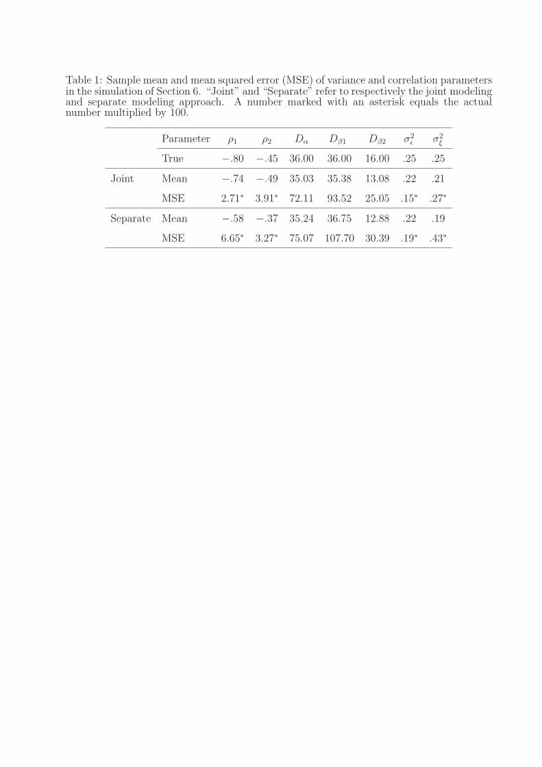
Table 1: Sample mean and mean squared error (MSE) of variance and correlation parametersin the simulation of Section 6. “Joint” and “Separate” refer to respectively the joint modelingand separate modeling approach. A number marked with an asterisk equals the actualnumber multiplied by 100.

Parameter ρ1 ρ2 Dα Dβ1 Dβ2 σ2ε σ2

ξ

True −.80 −.45 36.00 36.00 16.00 .25 .25

Joint Mean −.74 −.49 35.03 35.38 13.08 .22 .21

MSE 2.71∗ 3.91∗ 72.11 93.52 25.05 .15∗ .27∗

Separate Mean −.58 −.37 35.24 36.75 12.88 .22 .19

MSE 6.65∗ 3.27∗ 75.07 107.70 30.39 .19∗ .43∗

Table 2: Estimated variances of principal component scores for models with different numberof principal components in the AIDS example of Section 7. The variances are ordered indecreasing order for each model.

Number of principal comp. 1 2 3

Dα 99.6 122.1 7.8 128.7 9.7 (< 1e− 4)

Dβ 93.1 172.9 11.5 174.4 11.5 (< 1e− 4)

Table 3: Estimates of variance and correlation parameters and their 95% bootstrap confi-dence intervals in the AIDS example of Section 7. “Low” and “upper” represent the lowerand upper end points of the confidence intervals (CI).

parameter ρ1 ρ2 Dα Dβ1 Dβ2 σ2ε σ2

ξ

estimate −.35 .04 106.30 170.50 11.66 .25 .13

95% CI, low −.92 −.08 54.68 96.20 5.74 .20 .09

95% CI, upper −.05 .08 163.60 302.52 17.43 .30 .16

Figure 1: Fitted mean curves and principal component curves for five simulated data sets.Solid lines represent true curves.

0 20 40 60 80 100

1.0

1.5

2.0

2.5

Y, Mean curve

0 20 40 60 80 100−

0.5

0.0

0.5

1.0

Z, Mean curve

0 20 40 60 80 100

−0.

15−

0.10

−0.

050.

000.

050.

100.

15

Y, 1st PC

0 20 40 60 80 100

−0.

2−

0.1

0.0

0.1

0.2

Z, 1st PC

0 20 40 60 80 100

−0.

10.

00.

10.

2

Z, 2nd PC

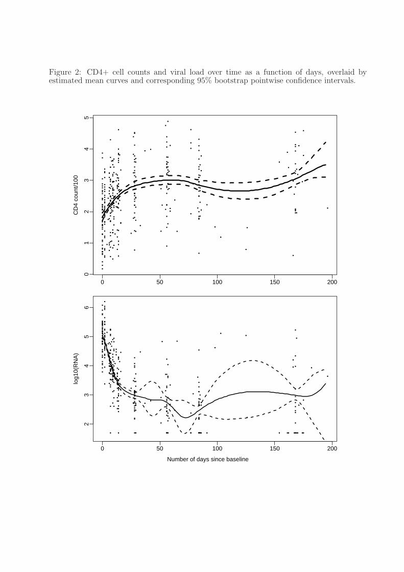
Figure 2: CD4+ cell counts and viral load over time as a function of days, overlaid byestimated mean curves and corresponding 95% bootstrap pointwise confidence intervals.

0 50 100 150 200

01

23

45

CD

4 co

unt/1

00

0 50 100 150 200

23

45

6

Number of days since baseline

log1

0(R

NA

)

Number of days since baseline

Figure 3: Left panels: Estimated principal component curves for CD4+ cell counts (top)and viral load (middle and bottom) with corresponding 95% pointwise confidence intervals.Right panels: Effect on the mean curves of adding and subtracting a multiple of each of theprincipal components shown on the left panels. The observed data are also shown on theright panels.

0 50 100 150 200

−0.

085

−0.

080

−0.

075

−0.

070

−0.

065

−0.

060

CD

4 co

unt/1

00, 1

st P

C

0 50 100 150 200

01

23

45

CD

4 co

unt/1

00

−−

−−−−−−−−−−−−−−−−−−−−−−−−−−−−−−−−−−−−−−−−−−−−−−−+

++

++++++++++++++++++++++++++++++++++++++++++++++

0 50 100 150 200

−0.

12−

0.10

−0.

08−

0.06

−0.

04−

0.02

0.00

log1

0(R

NA

), 1

st P

C

0 50 100 150 200

23

45

6

log1

0(R

NA

) −

−

−

−−

−−−−−−−−−−

−−

−−−−−−−−−−−−−−−−−−−−−−−−−−−−−−−−

+

+

++

++++++++++++

+++++

++

+++++++++++++++++++++++++

+

0 50 100 150 200−0.

15−

0.10

−0.

050.

000.

050.

10

log1

0(R

NA

), 2

nd P

C

0 50 100 150 200

23

45

6

log1

0(R

NA

)

−

−

−−

−−−−−−−−−−−−

−−−−−

−−−−−−−−−−−−−−−−−−−−−−−−−−

−−

+

+

+

+++++++++++

++

+++++++++++++++++++++++++++++++++

Number of days since baseline

Figure 4: Data and prediction of three selected subjects. Stars: observed values of (CD4 +count)/100 and log10(RNA). Solid lines: estimated mean curves. Dashed lines: individualbest linear unbiased predictions of the underlying curves.

0 50 100 150 200

01

23

45

Subject 1

CD

4 co

unt/1

00

*

**

** *

**

0 50 100 150 2001

23

45

6

Subject 1

log1

0(R

NA

)

*

***

* **

*

0 50 100 150 200

01

23

45

Subject 2

CD

4 co

unt/1

00

***

**

* **

*

0 50 100 150 200

12

34

56

Subject 2

log1

0(R

NA

)

**

**

** *

* *

0 50 100 150 200

01

23

45

Subject 3

CD

4 co

unt/1

00

**

*

*

*

** *

*

0 50 100 150 200

12

34

56

Subject 3

log1

0(R

NA

)

*****

* * * *