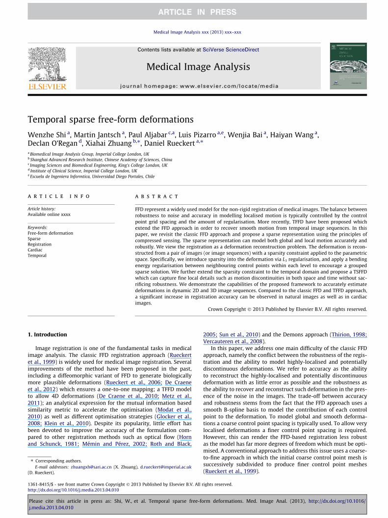
Medical Image Analysis xxx (2013) xxx–xxx

Contents lists available at SciVerse ScienceDirect

Medical Image Analysis

journal homepage: www.elsevier .com/locate /media

Temporal sparse free-form deformations

1361-8415/$ - see front matter Crown Copyright � 2013 Published by Elsevier B.V. All rights reserved.http://dx.doi.org/10.1016/j.media.2013.04.010

⇑ Corresponding authors.E-mail addresses: zhuangxh@sari.ac.cn (X. Zhuang), d.rueckert@imperial.ac.uk

(D. Rueckert).

Please cite this article in press as: Shi, W., et al. Temporal sparse free-form deformations. Med. Image Anal. (2013), http://dx.doi.org/1j.media.2013.04.010

Wenzhe Shi a, Martin Jantsch a, Paul Aljabar c,a, Luis Pizarro a,e, Wenjia Bai a, Haiyan Wang a,Declan O’Regan d, Xiahai Zhuang b,⇑, Daniel Rueckert a,⇑a Biomedical Image Analysis Group, Imperial College London, UKb Shanghai Advanced Research Institute, Chinese Academy of Sciences, Chinac Imaging Sciences and Biomedical Engineering, King’s College London, UKd Institute of Clinical Science, Imperial College London, UKe Escuela de Ingeniera Informtica, Universidad Diego Portales, Chile

a r t i c l e i n f o a b s t r a c t

Article history:Available online xxxx

Keywords:Free-form deformationSparseRegistrationCardiacTemporal

FFD represent a widely used model for the non-rigid registration of medical images. The balance betweenrobustness to noise and accuracy in modelling localised motion is typically controlled by the controlpoint grid spacing and the amount of regularisation. More recently, TFFD have been proposed whichextend the FFD approach in order to recover smooth motion from temporal image sequences. In thispaper, we revisit the classic FFD approach and propose a sparse representation using the principles ofcompressed sensing. The sparse representation can model both global and local motion accurately androbustly. We view the registration as a deformation reconstruction problem. The deformation is recon-structed from a pair of images (or image sequences) with a sparsity constraint applied to the parametricspace. Specifically, we introduce sparsity into the deformation via L1 regularisation, and apply a bendingenergy regularisation between neighbouring control points within each level to encourage a groupedsparse solution. We further extend the sparsity constraint to the temporal domain and propose a TSFFDwhich can capture fine local details such as motion discontinuities in both space and time without sac-rificing robustness. We demonstrate the capabilities of the proposed framework to accurately estimatedeformations in dynamic 2D and 3D image sequences. Compared to the classic FFD and TFFD approach,a significant increase in registration accuracy can be observed in natural images as well as in cardiacimages.

Crown Copyright � 2013 Published by Elsevier B.V. All rights reserved.

1. Introduction

Image registration is one of the fundamental tasks in medicalimage analysis. The classic FFD registration approach (Rueckertet al., 1999) is widely used for medical image registration. Severalimprovements of the method have been proposed in the past,including a diffeomorphic variant of FFD to generate biologicallymore plausible deformations (Rueckert et al., 2006; De Craeneet al., 2012) which ensures a one-to-one mapping; a TFFD modelto allow 4D deformations (De Craene et al., 2010; Metz et al.,2011); an analytical expression for the mutual information basedsimilarity metric to accelerate the optimisation (Modat et al.,2010) as well as different optimisation strategies (Glocker et al.,2008; Klein et al., 2010). Despite its popularity, little effort hasbeen devoted to improve the accuracy of the formulation com-pared to other registration methods such as optical flow (Hornand Schunck, 1981; Mémin and Pérez, 2002; Roth and Black,

2005; Sun et al., 2010) and the Demons approach (Thirion, 1998;Vercauteren et al., 2008).

In this paper, we address one main difficulty of the classic FFDapproach, namely the conflict between the robustness of the regis-tration and the ability to model highly-localised and potentiallydiscontinuous deformations. We refer to accuracy as the abilityto reconstruct the highly-localised and potentially discontinuousdeformation with as little error as possible and the robustness asthe ability to recover and reconstruct such deformation in the pres-ence of the noise in the images. The trade-off between accuracyand robustness stems from the fact that the FFD approach uses asmooth B-spline basis to model the contribution of each controlpoint to the deformation. To model global and smooth deforma-tions a coarse control point spacing is typically used. To allow verylocalised deformations a finer control point spacing is required.However, this can render the FFD-based registration less robustas the model has far more degrees of freedom which must be opti-mised. A conventional approach to address this issue uses a coarse-to-fine approach in which the initial coarse control point mesh issuccessively subdivided to produce finer control point meshes(Rueckert et al., 1999).

0.1016/

2 W. Shi et al. / Medical Image Analysis xxx (2013) xxx–xxx

The standard smoothness constraints for non-rigid registrationmethods (Rueckert et al., 1999; Horn and Schunck, 1981; Thirion,1998) assume that the deformation within a neighbourhoodchanges only gradually since the underlying deformation itself issmooth. Combining the implicit smoothness of the B-spline basisand the explicit smoothness constraint in the regularisation, leadsto FFD-based registration results with smooth deformations.

As mentioned above, the control point grid spacing has a signif-icant impact on the ability to capture motion discontinuities ro-bustly. Previous research focussed on the adaptiveparameterisation of the B-spline control point grid (Schnabelet al., 2001; Rohlfing and Maurer, 2001; Hansen et al., 2008) thathas been driven by the intensity information in the images. In addi-tion, Kumar et al. (2006) proposed to use shape prior informationand a shape dependent basis function to account for boundariesbetween foreground and background. An improved model shouldenable more control points to be placed in an area in which moreflexibility for the modelling of deformations is required. Xie andFarin (2004) proposed to use a distance measure to determinethe need for localised motion after initial registration using acoarse control point grid spacing.

Many other approaches to image registration have been pro-posed that aim to overcome the conflict between robustness andaccuracy in the motion estimation, in particular in the field of opti-cal flow estimation (Mémin and Pérez, 2002; Roth and Black, 2005;Sun et al., 2010). More recently, sparse coding methods have beenproposed to evaluate the patch similarity between two images(Roozgard et al., 2011) and to constrain the transformation (Shenand Wu, 2010). We address the trade-off between robustnessand accuracy for FFD-based registration by using sparsity con-straints as an additional regularization term.

FFD-based methods are now one of the most widely used meth-ods in recent cardiac motion tracking challenges (Tobon-Gomezet al., 2012; De Craene et al., 2013; Piella et al., 2013; Heydeet al., 2013). Among these approaches TFFD-based methods eitherbased on velocity fields (De Craene et al., 2010; De Craene et al.,2012; Piella et al., 2013) or based on displacement fields (Metzet al., 2011) have attracted increasing attention due to their abilityto extract consistent temporal motion pattern, which is importantfor estimation of cyclic motion such as the cardiac motion.

1.1. Overview and contributions

In this paper, we introduce a sparse representation for FFD toestimate the registration transformation. Our approach is inspiredby the work in Roozgard et al. (2011) and Shen and Wu (2010). Ourproposed model uses standard smoothness constraints and onlyimposes one additional assumption on the conventional FFD,namely that the deformation is sparse in the parametric space.Thus we call our method SFFD. The assumption of sparsity of thedeformation is generally true because the deformation betweenimages is usually less discontinuous than the actual images them-selves. In this work, we use a multi-level FFD model to representthe deformations in a parametric form. In this multi-level FFD eachlevel consists of a B-spline control point mesh with increasingly fi-ner resolution. As can be seen from Fig. 3, a dense motion field canbe represented by a sparse multi-level FFD in parametric space.Based on this assumption, we formulate the registration of twoimages using a sparse multi-level FFD representation of the controlpoints. We introduce a regularisation term to impose smoothnessat each level and a sparsity term to enforce coupled multi-levelsparsity. A preliminary version of this approach was published atMICCAI 2012 (Shi et al., 2012a).

In addition to the approach initially published in (Shi et al.,2012a), we extend the SFFD to the TSFFD based on the periodicTFFD (Metz et al., 2011) and apply it to the cardiac motion estima-

Please cite this article in press as: Shi, W., et al. Temporal sparse free-foj.media.2013.04.010

tion problem. TFFD refers to the implementation of (Metz et al.,2011) in the following sections. The extension to 4D enables usto better model the cyclic motion. It is well known that the diasta-sis and atrial systole phases, which are the final two phases of thediastole, occupy a disproportionably large time window in the car-diac cycle (Bray, 1999). Left ventricular myocardium undergoes lit-tle motion under these two phases. This means that thecontraction of the heart occurs in a relatively short time. Takenthat into account, the sparsity assumption is true in both the tem-poral and spatial domain in the context of the application to car-diac motion estimation.

The novelty and contributions of this paper are the introductionof a sparsity model that reduces the influence of the a priori selec-tion of an appropriate control point grid spacing. Furthermore, theapproach reduces the conflict between global smoothness (robust-ness) and the local level of detail of the transformation (accuracy)by optimising the different levels of the FFD coarser than the imageresolution level simultaneously with a sparsity constraint. Theseadvantages allow the robust estimation of deformation fields inthe presence of highly localised or discontinuous deformations inboth time and space. We refer to this new approach as SFFD in2D/3D and TSFFD in 4D. In the evaluation, we demonstrate thatthe proposed method can consistently capture all motion with highaccuracy in both 2D + t cases and 3D + t cases.

2. Datasets

In this work, we have evaluated the proposed SFFD and TSFFDagainst the classic FFD and TFFD model on four different datasets.The datasets we have used for evaluation include:

� The Middlebury benchmark dataset (Baker et al., 2007) (whichis a standard dataset widely used in computer vision);� 2D cardiac MR images with synthetic smooth motion. In the fol-

lowing this dataset will be referred to as Cardiac A;� 2D cardiac MR images with synthetic discontinuous motion. In

the following this dataset will be referred to as Cardiac B;� 10 synthetic but highly realistic 3D cardiac ultrasound image

sequences which have also been used in a recent cardiac motiontracking challenge (De Craene et al., 2013). In the following thisdataset will be referred to as Cardiac C.

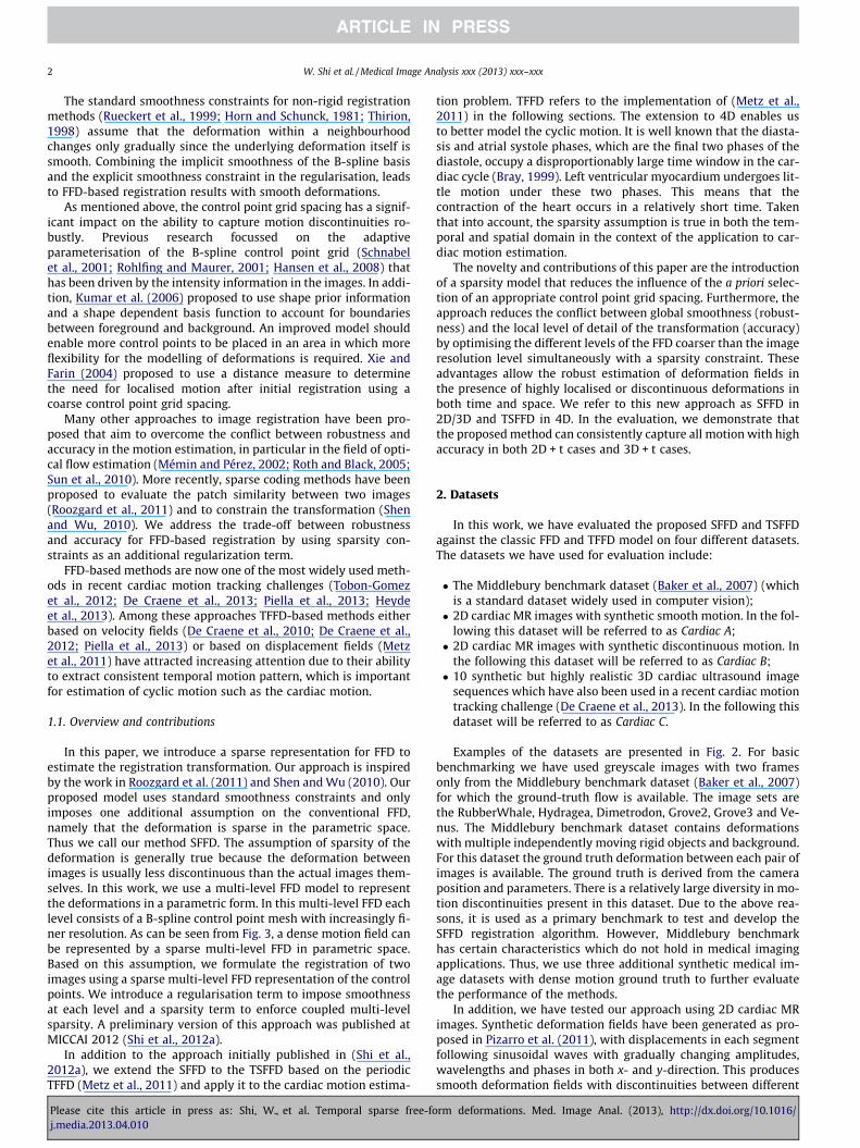
Examples of the datasets are presented in Fig. 2. For basicbenchmarking we have used greyscale images with two framesonly from the Middlebury benchmark dataset (Baker et al., 2007)for which the ground-truth flow is available. The image sets arethe RubberWhale, Hydragea, Dimetrodon, Grove2, Grove3 and Ve-nus. The Middlebury benchmark dataset contains deformationswith multiple independently moving rigid objects and background.For this dataset the ground truth deformation between each pair ofimages is available. The ground truth is derived from the cameraposition and parameters. There is a relatively large diversity in mo-tion discontinuities present in this dataset. Due to the above rea-sons, it is used as a primary benchmark to test and develop theSFFD registration algorithm. However, Middlebury benchmarkhas certain characteristics which do not hold in medical imagingapplications. Thus, we use three additional synthetic medical im-age datasets with dense motion ground truth to further evaluatethe performance of the methods.

In addition, we have tested our approach using 2D cardiac MRimages. Synthetic deformation fields have been generated as pro-posed in Pizarro et al. (2011), with displacements in each segmentfollowing sinusoidal waves with gradually changing amplitudes,wavelengths and phases in both x- and y-direction. This producessmooth deformation fields with discontinuities between different

rm deformations. Med. Image Anal. (2013), http://dx.doi.org/10.1016/

W. Shi et al. / Medical Image Analysis xxx (2013) xxx–xxx 3

segments. We generated two groups of 10 synthetic datasets each.The first group (Cardiac A) contains smooth motions created with asingle sinusoidal function over the whole image domain. The sec-ond group (Cardiac B) contains discontinuous motions created withmultiple sinusoidal functions fused together at different regions ofthe images. An example of this can be seen in Fig. 1b.

We have also used 10 synthetic cardiac ultrasound image se-quences from the second cardiac motion tracking challenge DeCraene et al. (2013) (Cardiac C). The synthetic image sequencesproposed in the challenge combine an electro-mechanical modelprovided by Sermesant et al. (2012) with an ultrasound imagingmodel from Gao et al. (2009). The challenge provides 10 highlyrealistic sequences spanning different values of the globalconductivity, global contractility, and electrical delays parameters.In the dataset, a single ultrasound probe design was considered.Scatterers were randomly placed in the myocardial geometry andmoved along the cardiac cycle according to the result of themechanical simulation. Details of the dataset can be found in DeCraene et al. (2013). The image resolution is approximately(0.34 � 0.34 � 0.34 mm) and the image sequence contains 23frames. Ground truth deformation is provided as a series of volu-metric meshes. The nodes of the meshes are landmarks coveringthe myocardium and give the ground truth deformation.

In all datasets, the accuracy is measured by the mean and SD ofthe distance between the ground truth motion and the recon-structed motion. In the dataset Cardiac C, we only evaluate theaccuracy in points inside the imaging area.

3. Classic free-form deformation model

In the classic FFD registration (Rueckert et al., 1999), a non-rigiddeformation h = [XYZ]T is represented using a B-spline model inwhich the deformation is parameterised using a set of controlpoints U = [UVW]T such that

h ¼B 0 00 B 00 0 B

264

375U; ð1Þ

Fig. 1. Visualisation of the sparse representation of a dense FFD using the colour schemreconstructed motion as the sum of (e) to (i); (d) colour scheme from (Baker et al., 2007)the references to colour in this figure legend, the reader is referred to the web version o

Please cite this article in press as: Shi, W., et al. Temporal sparse free-foj.media.2013.04.010

where B denotes the matrix of the B-spline basis functions. The B-spline basis function is a 3D-tensor product of 1D B-splines. Detailscan be found in Appendix A.

To find the optimal deformation between two images, the reg-istration minimises an energy functional E written as a functionof U, which is typically a combination of two terms E(U):¼ED(Ir,Is-

�h) + ER(U). The term ED is a data constraint measuring the similar-ity between the target image Ir and the transformed source imageIs�h. The term ER is a regularisation constraint that enforces asmooth transformation. In this classic FFD approach, the energyfunction is typically minimised using gradient descent approaches(Modat et al., 2010; Klein et al., 2010) or discrete optimisation ap-proaches (Glocker et al., 2008).

4. Sparse free-form deformation model

To be able to deal with large, global deformations and to im-prove the robustness, the classic FFD registration uses a multi-levelapproach: First, the optimal registration parameters are deter-mined for a control point grid with large spacing. The grid is thensuccessively subdivided to capture local deformations (Rueckertet al., 1999). This requires an a priori choice of the control pointgrid multi-resolution schedule. Furthermore, each level is opti-mised separately and once a level has been optimised it is no long-er updated, leading to suboptimal registration results as can beseen in Fig. 4. It was suggested in Shen and Wu (2010) that a real-istic transformation can be easily embedded into a sparse repre-sentation. We postulate that an automatic selection of controlpoints across different levels can be achieved by optimising allFFD levels simultaneously while using a sparsity constraint.

4.1. Sparse representation of transformation

In this section, we propose estimating the displacement h witha sparse representation of the control points U. We use a multi-le-vel FFD representation (Schnabel et al., 2001), U = [U1 � � � UmV1 -= [U1 � � � UmV1 � � � VmW1 � � �Wm]T where m denotes the number oflevels, as it is well suited for sparse representations. Accordingly,we utilise a multi-level B-splines basis B = [B1 � � � Bm]. The

e from (Baker et al., 2007): (a) Target image; (b) synthetic ground truth motion; (c); and (e–i) motion from FFD of different levels (coarse to fine). (For interpretation off this article.)

rm deformations. Med. Image Anal. (2013), http://dx.doi.org/10.1016/

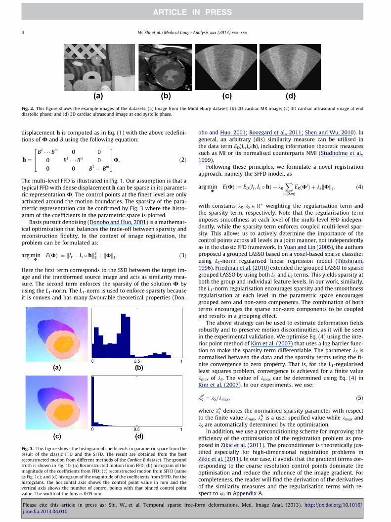
Fig. 2. This figure shows the example images of the datasets. (a) Image from the Middlebury dataset; (b) 2D cardiac MR image; (c) 3D cardiac ultrasound image at enddiastolic phase; and (d) 3D cardiac ultrasound image at end systolic phase.

4 W. Shi et al. / Medical Image Analysis xxx (2013) xxx–xxx

displacement h is computed as in Eq. (1) with the above redefini-tions of U and B using the following equation:

h ¼B1 � � �Bm 0 0

0 B1 � � �Bm 00 0 B1 � � �Bm

264

375U; ð2Þ

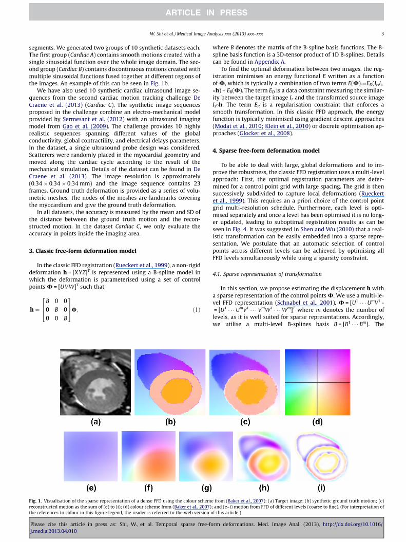
The multi-level FFD is illustrated in Fig. 1. Our assumption is that atypical FFD with dense displacement h can be sparse in its paramet-ric representation U. The control points at the finest level are onlyactivated around the motion boundaries. The sparsity of the para-metric representation can be confirmed by Fig. 3 where the histo-gram of the coefficients in the parametric space is plotted.

Basis pursuit denoising (Donoho and Huo, 2001) is a mathemat-ical optimisation that balances the trade-off between sparsity andreconstruction fidelity. In the context of image registration, theproblem can be formulated as:

arg minU

EðUÞ :¼ kIr � Is � hk22 þ kUk1; ð3Þ

Here the first term corresponds to the SSD between the target im-age and the transformed source image and acts as similarity mea-sure. The second term enforces the sparsity of the solution U byusing the L1-norm. The L1-norm is used to enforce sparsity becauseit is convex and has many favourable theoretical properties (Don-

Fig. 3. This figure shows the histogram of coefficients in parametric space from theresult of the classic FFD and the SFFD. The result are obtained from the bestreconstructed motion from different methods of the Cardiac B dataset. The groundtruth is shown in Fig. 1b. (a) Reconstructed motion from FFD; (b) histogram of themagnitude of the coefficients from FFD; (c) reconstructed motion from SFFD (sameas Fig. 1c); and (d) histogram of the magnitude of the coefficients from SFFD. For thehistograms, the horizontal axis shows the control point value in mm and thevertical axis shows the number of control points with that binned control pointvalue. The width of the bins is 0.05 mm.

Please cite this article in press as: Shi, W., et al. Temporal sparse free-foj.media.2013.04.010

oho and Huo, 2001; Roozgard et al., 2011; Shen and Wu, 2010). Ingeneral, an arbitrary (dis) similarity measure can be utilised inthe data term ED(Ir, Is�h), including information theoretic measuressuch as MI or its normalised counterparts NMI (Studholme et al.,1999).

Following these principles, we formulate a novel registrationapproach, namely the SFFD model, as

arg minU

EðUÞ :¼ EDðIr ; Is � hÞ þ kR

Xi2½0;m�

ERðUiÞ þ kSkUk1; ð4Þ

with constants kR; kS 2 Rþ weighting the regularisation term andthe sparsity term, respectively. Note that the regularisation termimposes smoothness at each level of the multi-level FFD indepen-dently, while the sparsity term enforces coupled multi-level spar-sity. This allows us to actively determine the importance of thecontrol points across all levels in a joint manner, not independentlyas in the classic FFD framework. In Yuan and Lin (2005), the authorsproposed a grouped LASSO based on a voxel-based sparse classifierusing L1-norm regularised linear regression model (Tibshirani,1996). Friedman et al. (2010) extended the grouped LASSO to sparsegrouped LASSO by using both L1 and L2 terms. This yields sparsity atboth the group and individual feature levels. In our work, similarly,the L1-norm regularisation encourages sparsity and the smoothnessregularisation at each level in the parametric space encouragesgrouped zero and non-zero components. The combination of bothterms encourages the sparse non-zero components to be coupledand results in a grouping effect.

The above strategy can be used to estimate deformation fieldsrobustly and to preserve motion discontinuities, as it will be seenin the experimental validation. We optimise Eq. (4) using the inte-rior point method of Kim et al. (2007) that uses a log barrier func-tion to make the sparsity term differentiable. The parameter kS isnormalised between the data and the sparsity terms using the fi-nite convergence to zero property. That is, for the L1-regularisedleast squares problem, convergence is achieved for a finite valuekmax of kS. The value of kmax can be determined using Eq. (4) inKim et al. (2007). In our experiments, we use:

kNS ¼ kS=kmax; ð5Þ

where kNS denotes the normalised sparsity parameter with respect

to the finite value kmax. kNS is a user specified value while kmax and

kS are automatically determined by the optimisation.In addition, we use a preconditioning scheme for improving the

efficiency of the optimisation of the registration problem as pro-posed in Zikic et al. (2011). The preconditioner is theoretically jus-tified especially for high-dimensional registration problems inZikic et al. (2011). In our case, it avoids that the gradient terms cor-responding to the coarse resolution control points dominate theoptimisation and reduce the influence of the image gradient. Forcompleteness, the reader will find the derivation of the derivativesof the similarity measures and the regularisation terms with re-spect to /i in Appendix A.

rm deformations. Med. Image Anal. (2013), http://dx.doi.org/10.1016/

W. Shi et al. / Medical Image Analysis xxx (2013) xxx–xxx 5

5. Temporal sparse free-form deformation model

To extend the classic FFD registration method, as described inSection 3 to model the cyclic deformationh ¼ ½X0 � � �XNt Y0 � � �YNt Z0 � � � ZNt �

T in an image sequence with Nt

temporal frames denoted by Ilr for l = 1, . . . , Nt, we construct a set

of 4D control points with coefficients U ¼ U10 � � �U

1t1� � �Um

0 � � �Umtm

hV1

0 � � �V1t1� � �Vm

0 � � �Vmtm

W10 � � �W

1t1� � �Wm

0 � � �Wmtm�T . We have m 4D

control point meshes, and each one with temporal resolution tk.The first and last spatial control points are defined to be directneighbours to enforce cyclic motion (Metz et al., 2011). When reg-istering cardiac sequences the periodicity of the model ensures atemporally smooth motion. For other cases this neighbourhooddefinition can be easily modified. This lead to the followingequation:

h¼B1

0 � � �B1t1� � �Bm

0 � � �Bmtm

0 00 B1

0 � � �B1t1� � �Bm

0 � � �Bmtm

00 0 B1

0 � � �B1t1� � �Bm

0 � � �Bmtm

264

375U; ð6Þ

The matrix B in Eq. (6) now consists of B-spline basis functions de-fined by a 4D-tensor product. Note that in this definition, there is nocomponent of the deformation in the temporal direction. Thismeans we use a 4D mesh of control points and each control pointis a 3D displacement vector. There are cases where this might notbe true, e.g. because of temporal misalignment due to variabilityin the cardiac cycle. In these cases, the approach of (Perperidiset al., 2005) can be used to perform an interleaved spatial and tem-poral optimisation to correct 4D displacement field.

The TFFD registration method also uses a multi-level approachas described in Section 4, but with a constant temporal spacing.However, to make use of the temporal sparsity of the motion,our TSFFD method uses multiple grid spacings for all four dimen-sions. To be able to make use of the full parametric space, we needto subdivide the spatial and temporal grid spacing independently.Then combinations between all spatial resolutions and every tem-poral resolution should be used. This is necessary because the car-diac contraction occurs during a very short period of the cardiaccycle and there might be some temporally consistent but spatiallydiscontinuous motion (for example the sliding motion that occursat the pericardium) over the whole cardiac cycle. However, in prac-tice, it is not computational feasible and very memory intensive.Thus, we choose to subdivide the spatial control point mesh be-tween levels.

The definition of the control points U and the B-spline basismatrix for the TFFD model is straightforward. Following the defini-

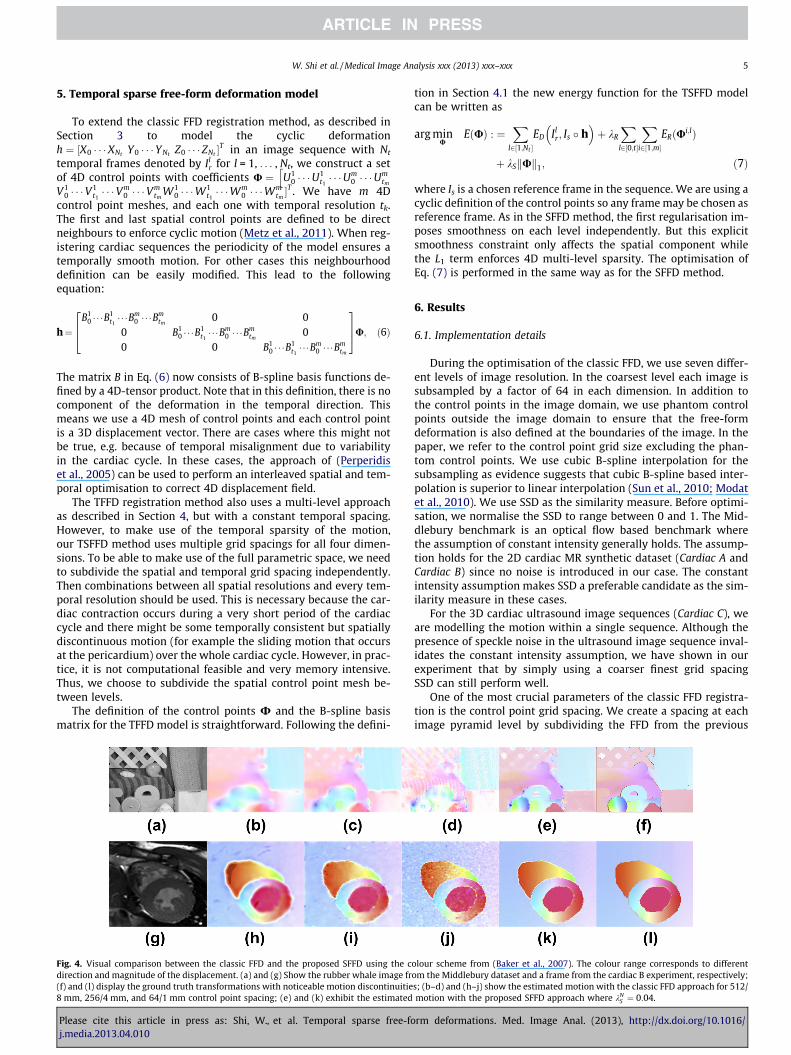
Fig. 4. Visual comparison between the classic FFD and the proposed SFFD using the cdirection and magnitude of the displacement. (a) and (g) Show the rubber whale image fr(f) and (l) display the ground truth transformations with noticeable motion discontinuitie8 mm, 256/4 mm, and 64/1 mm control point spacing; (e) and (k) exhibit the estimated

Please cite this article in press as: Shi, W., et al. Temporal sparse free-foj.media.2013.04.010

tion in Section 4.1 the new energy function for the TSFFD modelcan be written as

arg minU

EðUÞ : ¼X

l2½1;Nt �ED Il

r; Is � h� �

þ kR

Xl2½0;t�

Xi2½1;m�

ERðUi;lÞ

þ kSkUk1; ð7Þ

where Is is a chosen reference frame in the sequence. We are using acyclic definition of the control points so any frame may be chosen asreference frame. As in the SFFD method, the first regularisation im-poses smoothness on each level independently. But this explicitsmoothness constraint only affects the spatial component whilethe L1 term enforces 4D multi-level sparsity. The optimisation ofEq. (7) is performed in the same way as for the SFFD method.

6. Results

6.1. Implementation details

During the optimisation of the classic FFD, we use seven differ-ent levels of image resolution. In the coarsest level each image issubsampled by a factor of 64 in each dimension. In addition tothe control points in the image domain, we use phantom controlpoints outside the image domain to ensure that the free-formdeformation is also defined at the boundaries of the image. In thepaper, we refer to the control point grid size excluding the phan-tom control points. We use cubic B-spline interpolation for thesubsampling as evidence suggests that cubic B-spline based inter-polation is superior to linear interpolation (Sun et al., 2010; Modatet al., 2010). We use SSD as the similarity measure. Before optimi-sation, we normalise the SSD to range between 0 and 1. The Mid-dlebury benchmark is an optical flow based benchmark wherethe assumption of constant intensity generally holds. The assump-tion holds for the 2D cardiac MR synthetic dataset (Cardiac A andCardiac B) since no noise is introduced in our case. The constantintensity assumption makes SSD a preferable candidate as the sim-ilarity measure in these cases.

For the 3D cardiac ultrasound image sequences (Cardiac C), weare modelling the motion within a single sequence. Although thepresence of speckle noise in the ultrasound image sequence inval-idates the constant intensity assumption, we have shown in ourexperiment that by simply using a coarser finest grid spacingSSD can still perform well.

One of the most crucial parameters of the classic FFD registra-tion is the control point grid spacing. We create a spacing at eachimage pyramid level by subdividing the FFD from the previous

olour scheme from (Baker et al., 2007). The colour range corresponds to differentom the Middlebury dataset and a frame from the cardiac B experiment, respectively;s; (b–d) and (h–j) show the estimated motion with the classic FFD approach for 512/motion with the proposed SFFD approach where kN

S ¼ 0:04.

rm deformations. Med. Image Anal. (2013), http://dx.doi.org/10.1016/

6 W. Shi et al. / Medical Image Analysis xxx (2013) xxx–xxx

level. For the Middlebury dataset as well as Cardiac A and Cardiac Bdatasets, we have evaluated different initial control point spacingsat the coarsest level varying from 512 mm to 64 mm while the con-trol point spacings at the final level varies from 8 mm to 1 mm. Thespacing at the coarser level is subdivided by a factor of 2 to createthe finer level. For the SFFD, we use a multi-level FFD with thecoarsest level having a control point grid spacing of 64 mm and fin-est level having a spacing of 1 mm. The number of control points ofSFFD at coarsest level is 4 � 4. During the optimisation, SFFD con-trol point resolutions are only activated on levels which are coarserthan the current image resolution. The coefficient for the smooth-ness penalty is set to 0.01 as in (Rueckert et al., 1999). The numberof image pyramid levels and the smoothness penalty kR are thesame for both methods.

For cardiac C dataset, we use four different levels of image res-olution. The first image of the ED phase is used as the reference im-age. In the coarsest level each image is subsampled by a factor ofsixteen in each dimension. In the finest level, each image is sub-sampled by a factor of two in each dimension to reduce the com-putational expense. In this dataset, we use relatively coarser

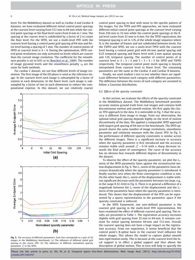
Fig. 5. The accuracy of different parameters. Each line corresponds to a pair of 2Dimages in the Middlebury benchmark. (a) The influence of different initial gridspacing to the classic FFD. (b) The influence of different normalised sparsityparameter kN

S to the SFFD.

Please cite this article in press as: Shi, W., et al. Temporal sparse free-foj.media.2013.04.010

control point spacing to deal with noise in the speckle pattern ofthe images. For the TFFD and FFD approaches, we have evaluateddifferent initial control point spacings at the coarsest level varyingfrom 256 mm to 32 mm while the control point spacings at the fi-nal level varies from 32 mm to 4 mm. For the TFFD registration, thetemporal spacing is set to 1/Nt of the whole image sequence whereNt is the number of frames and not subdivided between levels. Forthe TSFFD and SFFD, we use a multi-level TFFD with the coarsestlevel having a control point grid with 64 mm spatial spacing and0.25 temporal spacing and finest level with 2 mm spatial spacingand 1/Nt temporal spacing. The number of control points of atcoarsest level is 3 � 3 � 3 and 3 � 3 � 3 � 5 for SFFD and TSFFDrespectively. The temporal control point mesh spacing is linearlyinterpolated from coarsest level to finest level. The remainingparameters are the same as the Cardiac A and Cardiac B datasets.

Finally, we used student t-test to test whether there are signif-icant difference between each category with different parameters.The difference between the errors of each category are assumed tofollow a Gaussian distribution.

6.2. Effects of the sparsity constraint

In this section, we evaluate the effects of the sparsity constraintin the Middlebury dataset. The Middlebury benchmark providesaccurate motion ground truth from real images and contains bothdiscontinuous motion and smooth motion. We first apply the clas-sic FFD approach to the data. It is noticeable in Fig. 5 that the accu-racy is different from image to image. From our observation, theoptimal initial grid spacing depends highly on the level of motiondiscontinuity of the data. We applied a comparable SFFD approachwith largest grid spacing of 64 mm to the benchmark. The SFFD ap-proach shares the same number of image resolutions, smoothnessparameter and similarity measure with the classic FFD. In Fig. 5,the performance of different sparsity constraints is similar acrossthe different images. There is a significant increase in accuracywhen the sparsity parameter is first introduced and the accuracyremains stable until around kN

S ¼ 0:16 with a sharp decrease to-wards the final point of convergence. The curve of the accuracyhas no obvious bias towards different degrees of discontinuity inthe dataset.

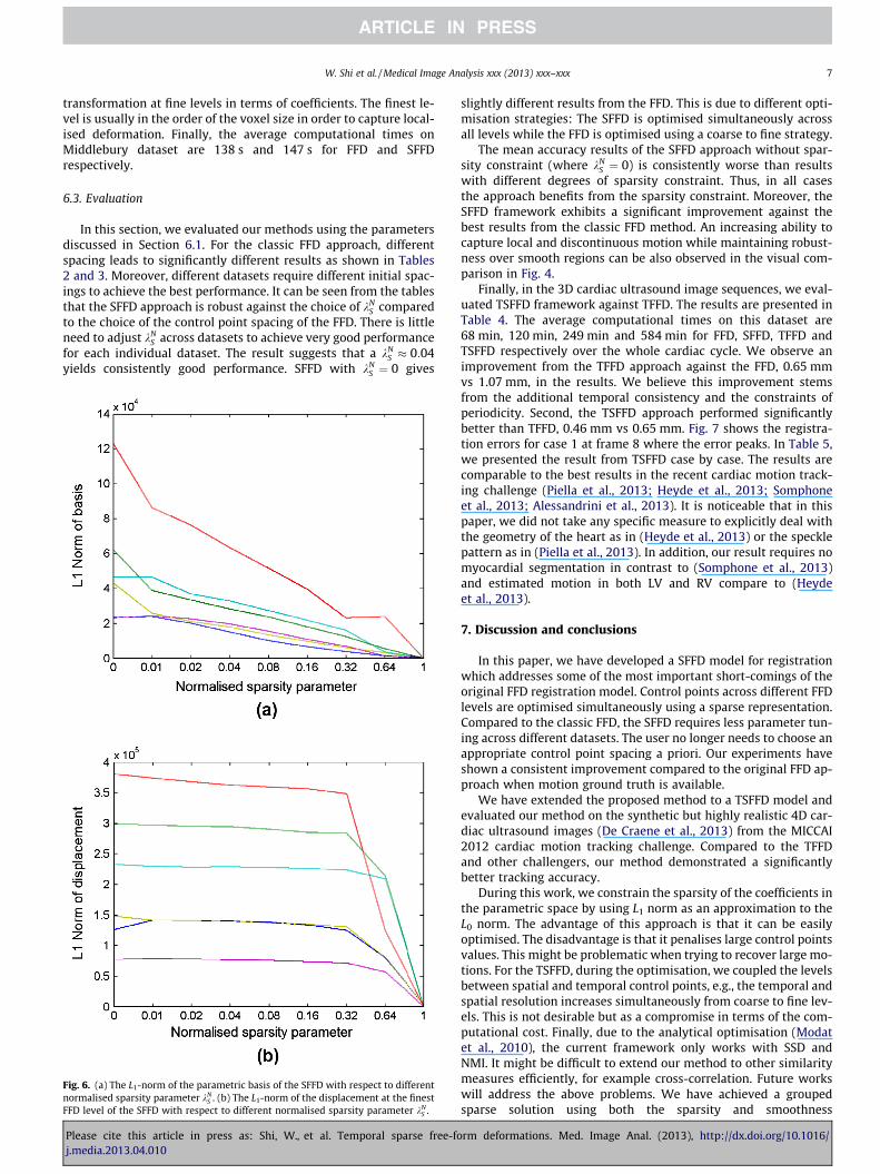
To observe the effect of the sparsity parameter, we plot the L1-norm of the SFFD parametric basis against the reconstructed mo-tion displacement in Fig. 6. The L1-norm of the parametric basis de-creases dramatically when the sparsity parameter is introduced. Itfinally reaches zero when the finite convergence condition is met.On the other hand, the L1-norm of the displacement is stable with-out significant decrease until the parameter becomes too large, e.g.,in the range 0.32–0.64 in Fig. 6. There is in general a difference of amagnitude between the L1-norm of the displacement and the L1-norm of the parametric basis when the sparsity parameter is intro-duced. This shows that the displacement of the FFD can be repre-sented by a sparse representation in the parametric space if thesparsity constraint is enforced.

In the SFFD framework, one user-defined parameter is thecoarsest grid spacing in the multi-level FFD representation. Wehave examined the effect of different coarsest grid spacing. The re-sults are presented in Table 1. The registration accuracy increasesslightly with grid spacing from 32 mm to 64 mm. It remains con-stant for initial spacing between 64 mm and 512 mm. Overall,the coarsest spacing does not have a huge impact on the registra-tion accuracy. From our experience, it seems beneficial that thecontrol point’s B-spline basis in the coarsest level influence thewhole images. This allows the model to capture global smoothnon-rigid motion easily. This is because at the coarsest level the lo-cal support is in effect a global support and thus allows thedescription of global motion. This in turn will help to sparsify the

rm deformations. Med. Image Anal. (2013), http://dx.doi.org/10.1016/

W. Shi et al. / Medical Image Analysis xxx (2013) xxx–xxx 7

transformation at fine levels in terms of coefficients. The finest le-vel is usually in the order of the voxel size in order to capture local-ised deformation. Finally, the average computational times onMiddlebury dataset are 138 s and 147 s for FFD and SFFDrespectively.

6.3. Evaluation

In this section, we evaluated our methods using the parametersdiscussed in Section 6.1. For the classic FFD approach, differentspacing leads to significantly different results as shown in Tables2 and 3. Moreover, different datasets require different initial spac-ings to achieve the best performance. It can be seen from the tablesthat the SFFD approach is robust against the choice of kN

S comparedto the choice of the control point spacing of the FFD. There is littleneed to adjust kN

S across datasets to achieve very good performancefor each individual dataset. The result suggests that a kN

S � 0:04yields consistently good performance. SFFD with kN

S ¼ 0 gives

Fig. 6. (a) The L1-norm of the parametric basis of the SFFD with respect to differentnormalised sparsity parameter kN

S . (b) The L1-norm of the displacement at the finestFFD level of the SFFD with respect to different normalised sparsity parameter kN

S .

Please cite this article in press as: Shi, W., et al. Temporal sparse free-foj.media.2013.04.010

slightly different results from the FFD. This is due to different opti-misation strategies: The SFFD is optimised simultaneously acrossall levels while the FFD is optimised using a coarse to fine strategy.

The mean accuracy results of the SFFD approach without spar-sity constraint (where kN

S ¼ 0) is consistently worse than resultswith different degrees of sparsity constraint. Thus, in all casesthe approach benefits from the sparsity constraint. Moreover, theSFFD framework exhibits a significant improvement against thebest results from the classic FFD method. An increasing ability tocapture local and discontinuous motion while maintaining robust-ness over smooth regions can be also observed in the visual com-parison in Fig. 4.

Finally, in the 3D cardiac ultrasound image sequences, we eval-uated TSFFD framework against TFFD. The results are presented inTable 4. The average computational times on this dataset are68 min, 120 min, 249 min and 584 min for FFD, SFFD, TFFD andTSFFD respectively over the whole cardiac cycle. We observe animprovement from the TFFD approach against the FFD, 0.65 mmvs 1.07 mm, in the results. We believe this improvement stemsfrom the additional temporal consistency and the constraints ofperiodicity. Second, the TSFFD approach performed significantlybetter than TFFD, 0.46 mm vs 0.65 mm. Fig. 7 shows the registra-tion errors for case 1 at frame 8 where the error peaks. In Table 5,we presented the result from TSFFD case by case. The results arecomparable to the best results in the recent cardiac motion track-ing challenge (Piella et al., 2013; Heyde et al., 2013; Somphoneet al., 2013; Alessandrini et al., 2013). It is noticeable that in thispaper, we did not take any specific measure to explicitly deal withthe geometry of the heart as in (Heyde et al., 2013) or the specklepattern as in (Piella et al., 2013). In addition, our result requires nomyocardial segmentation in contrast to (Somphone et al., 2013)and estimated motion in both LV and RV compare to (Heydeet al., 2013).

7. Discussion and conclusions

In this paper, we have developed a SFFD model for registrationwhich addresses some of the most important short-comings of theoriginal FFD registration model. Control points across different FFDlevels are optimised simultaneously using a sparse representation.Compared to the classic FFD, the SFFD requires less parameter tun-ing across different datasets. The user no longer needs to choose anappropriate control point spacing a priori. Our experiments haveshown a consistent improvement compared to the original FFD ap-proach when motion ground truth is available.

We have extended the proposed method to a TSFFD model andevaluated our method on the synthetic but highly realistic 4D car-diac ultrasound images (De Craene et al., 2013) from the MICCAI2012 cardiac motion tracking challenge. Compared to the TFFDand other challengers, our method demonstrated a significantlybetter tracking accuracy.

During this work, we constrain the sparsity of the coefficients inthe parametric space by using L1 norm as an approximation to theL0 norm. The advantage of this approach is that it can be easilyoptimised. The disadvantage is that it penalises large control pointsvalues. This might be problematic when trying to recover large mo-tions. For the TSFFD, during the optimisation, we coupled the levelsbetween spatial and temporal control points, e.g., the temporal andspatial resolution increases simultaneously from coarse to fine lev-els. This is not desirable but as a compromise in terms of the com-putational cost. Finally, due to the analytical optimisation (Modatet al., 2010), the current framework only works with SSD andNMI. It might be difficult to extend our method to other similaritymeasures efficiently, for example cross-correlation. Future workswill address the above problems. We have achieved a groupedsparse solution using both the sparsity and smoothness

rm deformations. Med. Image Anal. (2013), http://dx.doi.org/10.1016/

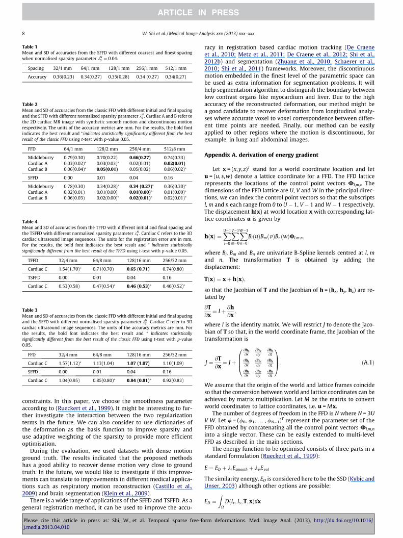
Table 2Mean and SD of accuracies from the classic FFD with different initial and final spacingand the SFFD with different normalised sparsity parameter kN

S . Cardiac A and B refer tothe 2D cardiac MR image with synthetic smooth motion and discontinuous motionrespectively. The units of the accuracy metrics are mm. For the results, the bold fontindicates the best result and ⁄ indicates statistically significantly different from the bestresult of the classic FFD using t-test with p-value 0.05.

FFD 64/1 mm 128/2 mm 256/4 mm 512/8 mm

Middleburry 0.79(0.30) 0.70(0.22) 0.66(0.27) 0.74(0.33)Cardiac A 0.03(0.02)⁄ 0.03(0.03)⁄ 0.02(0.01) 0.02(0.01)Cardiac B 0.06(0.04)⁄ 0.05(0.01) 0.05(0.02) 0.06(0.02)⁄

SFFD 0.00 0.01 0.04 0.16

Middleburry 0.78(0.30) 0.34(0.28)⁄ 0.34 (0.27)⁄ 0.36(0.30)⁄

Cardiac A 0.02(0.01) 0.01(0.00) 0.01(0.00)⁄ 0.01(0.00)⁄

Cardiac B 0.06(0.03) 0.02(0.00)⁄ 0.02(0.01)⁄ 0.02(0.01)⁄

Table 3Mean and SD of accuracies from the classic FFD with different initial and final spacingand the SFFD with different normalised sparsity parameter kN

S . Cardiac C refer to 3Dcardiac ultrasound image sequences. The units of the accuracy metrics are mm. Forthe results, the bold font indicates the best result and ⁄ indicates statisticallysignificantly different from the best result of the classic FFD using t-test with p-value0.05.

FFD 32/4 mm 64/8 mm 128/16 mm 256/32 mm

Cardiac C 1.57(1.12)⁄ 1.13(1.04) 1.07 (1.07) 1.10(1.09)

SFFD 0.00 0.01 0.04 0.16

Cardiac C 1.04(0.95) 0.85(0.80)⁄ 0.84 (0.81)⁄ 0.92(0.83)

Table 1Mean and SD of accuracies from the SFFD with different coarsest and finest spacingwhen normalised sparsity parameter kN

S ¼ 0:04.

Spacing 32/1 mm 64/1 mm 128/1 mm 256/1 mm 512/1 mm

Accuracy 0.36(0.23) 0.34(0.27) 0.35(0.28) 0.34 (0.27) 0.34(0.27)

Table 4Mean and SD of accuracies from the TFFD with different initial and final spacing andthe TSFFD with different normalised sparsity parameter kN

S . Cardiac C refers to the 3Dcardiac ultrasound image sequences. The units for the registration error are in mm.For the results, the bold font indicates the best result and * indicates statisticallysignificantly different from the best result of the TFFD using t-test with p-value 0.05.

TFFD 32/4 mm 64/8 mm 128/16 mm 256/32 mm

Cardiac C 1.54(1.70)⁄ 0.71(0.70) 0.65 (0.71) 0.74(0.80)

TSFFD 0.00 0.01 0.04 0.16

Cardiac C 0.53(0.58) 0.47(0.54)⁄ 0.46 (0.53)⁄ 0.46(0.52)⁄

8 W. Shi et al. / Medical Image Analysis xxx (2013) xxx–xxx

constraints. In this paper, we choose the smoothness parameteraccording to (Rueckert et al., 1999). It might be interesting to fur-ther investigate the interaction between the two regularizationterms in the future. We can also consider to use dictionaries ofthe deformation as the basis function to improve sparsity anduse adaptive weighting of the sparsity to provide more efficientoptimisation.

During the evaluation, we used datasets with dense motionground truth. The results indicated that the proposed methodshas a good ability to recover dense motion very close to groundtruth. In the future, we would like to investigate if this improve-ments can translate to improvements in different medical applica-tions such as respiratory motion reconstruction (Castillo et al.,2009) and brain segmentation (Klein et al., 2009).

There is a wide range of applications of the SFFD and TSFFD. As ageneral registration method, it can be used to improve the accu-

Please cite this article in press as: Shi, W., et al. Temporal sparse free-foj.media.2013.04.010

racy in registration based cardiac motion tracking (De Craeneet al., 2010; Metz et al., 2011; De Craene et al., 2012; Shi et al.,2012b) and segmentation (Zhuang et al., 2010; Schaerer et al.,2010; Shi et al., 2011) frameworks. Moreover, the discontinuousmotion embedded in the finest level of the parametric space canbe used as extra information for segmentation problems. It willhelp segmentation algorithm to distinguish the boundary betweenlow contrast organs like myocardium and liver. Due to the highaccuracy of the reconstructed deformation, our method might bea good candidate to recover deformation from longitudinal analy-ses where accurate voxel to voxel correspondence between differ-ent time points are needed. Finally, our method can be easilyapplied to other regions where the motion is discontinuous, forexample, in lung and abdominal images.

Appendix A. derivation of energy gradient

Let x = (x,y,z)T stand for a world coordinate location and letu = (u,v,w) denote a lattice coordinate for a FFD. The FFD latticerepresents the locations of the control point vectors Ul,m,n Thedimensions of the FFD lattice are U, V and W in the principal direc-tions, we can index the control point vectors so that the subscriptsl, m and n each range from 0 to U � 1, V � 1 and W � 1 respectively.The displacement h(x) at world location x with corresponding lat-tice coordinates u is given by

hðxÞ ¼XU�1

l¼0

XV�1

m¼0

XW�1

n¼0

BlðuÞBmðvÞBnðwÞUl;m;n;

where Bl, Bm and Bn are univariate B-Spline kernels centred at l, mand n. The transformation T is obtained by adding thedisplacement:

TðxÞ ¼ xþ hðxÞ;

so that the Jacobian of T and the Jacobian of h = (hx, hy, hz) are re-lated by

@T@x¼ I þ @h

@x;

where I is the identity matrix. We will restrict J to denote the Jaco-bian of T so that, in the world coordinate frame, the Jacobian of thetransformation is

J ¼ @T@x¼ I þ

@hx@x

@hx@y

@hx@z

@hy

@x@hy

@y@hy

@z

@hz@x

@hz@y

@hz@z

0BB@

1CCA: ðA:1Þ

We assume that the origin of the world and lattice frames coincideso that the conversion between world and lattice coordinates can beachieved by matrix multiplication. Let M be the matrix to convertworld coordinates to lattice coordinates, i.e. u = Mx.

The number of degrees of freedom in the FFD is N where N = 3UV W. Let / = (/0, /1, . . . , /N�1)T represent the parameter set of theFFD obtained by concatenating all the control point vectors Ul,m,n

into a single vector. These can be easily extended to multi-levelFFD as described in the main sections.

The energy function to be optimised consists of three parts in astandard formulation (Rueckert et al., 1999):

E ¼ ED þ krEsmooth þ kvEvol

The similarity energy, ED is considered here to be the SSD (Kybic andUnser, 2003) although other options are possible:

ED ¼Z

XDðIr; Is;T;xÞdx

rm deformations. Med. Image Anal. (2013), http://dx.doi.org/10.1016/

Table 5Mean and SD of accuracies from the TSFFD with kN

S ¼ 0:04. The results concern theCardiac C data and the numbering refers to the original numbering in the challenge.The units of the accuracy are mm

ID 01 08 12 20 22 28 36 44 60 88

Mean 0.71 0.37 0.39 0.39 0.66 0.39 0.38 0.47 0.42 0.38SD 0.78 0.37 0.41 0.38 0.74 0.40 0.39 0.49 0.41 0.55

Fig. 7. Visualisation of the registration error for case 1 (lateral view) at frame 8 from cardiac C dataset. The colour overlay on the deformed ground-truth mesh represents themagnitude of the registration error (mm). (a) and (f) Show the ultrasound image from frame 1 and 8, respectively; (b–e) show the error map from the TFFD approach with 32/4 mm, 64/8 mm, 128/16 mm and 256/32 mm control point spacing and (g–j) show the error map from the TSFFD approach with kN

S ¼ 0kNS ¼ 0:01kN

S ¼ 0:04 and kNS ¼ 0:16. (For

interpretation of the references to colour in this figure legend, the reader is referred to the web version of this article.)

W. Shi et al. / Medical Image Analysis xxx (2013) xxx–xxx 9

where X is a fixed region of interest and D(Ir, Is,T,x) = (Ir(x)� Is(T(x)))2 is the SSD between target image Ir and source image Is

after applying transformation T at point x. We require the gradientof this energy ED with respect to the deformation parameters andwe assume that D(Ir, Is,T,x), as a function of the components of /

and x, satisfies the conditions for differentiation under the integralsign. This means that we can write

@ED

@/¼Z

X

@DðIr; Is;T; xÞ@/

dx ðA:2Þ

The derivative of the integrand is readily found in Kybic and Unser(2003)

@

@/iðIrðxÞ � IsðTðxÞÞÞ2 ¼

@ðIrðxÞ � IsðTðxÞÞÞ2

@IsðTðxÞÞ@IsðTðxÞÞ@TðxÞ

@TðxÞ@/i

¼ 2ðIrðxÞ � IsðTðxÞÞÞ rIs � Tjx@TðxÞ@/i

: ðA:3Þ

The smooth preservation energy is a spatially integrated function ofthe bending energy:

Esmooth ¼1jXj

ZX

@2T@x2

!2

þ @2T@y2

!2

þ @2T@z2

!224

35dx ðA:4Þ

þ 1jXj

ZX

2@2T@xy

!2

þ 2@2T@xz

!2

þ 2@2T@yz

!224

35dx ðA:5Þ

where jXj is the size of the region. We require the gradient of thisenergy with respect to the deformation parameters. AbbreviatingEq. (A.5) as Esmooth ¼ 1

jXjR

X½A2 þ B2 þ C2 þ 2D2 þ 2E2 þ 2F2�dx, the

derivative of the penalty term with respect to a deformation param-eter /i involves a sum of derivatives each of which can be obtainedusing the chain rule, e.g. @ðA

2Þ@/i¼ 2A @A

@/i. The same chain rule can be ap-

plied to each and every component of the Eq. (A.5).

Please cite this article in press as: Shi, W., et al. Temporal sparse free-foj.media.2013.04.010

Finally, the volume preservation energy is a spatially integratedfunction of the determinant of the Jacobian, J:

Evol ¼Z

Xðlog jJjÞ2dx

where j � j denotes the determinant of J. We require the gradient ofthis energy with respect to the deformation parameters and we as-sume that (log (jJj))2, as a function of the components of / and x,satisfies the conditions for differentiation under the integral sign.This means that we can write

@Evol

@/¼Z

X

@ logðjJjÞ2

@/dx ðA:6Þ

Differentiating the integrand, we obtain

@ðlog jJjÞ2

@/¼ 2 log jJj

jJj@jJj@/

: ðA:7Þ

jJj and its logarithm are readily calculated so we require an expres-sion for the gradient @jJj

@/. The ith component of the @jJj

@/is given by

@jJj@/i¼ tr adjðJÞ @J

@/i

� �

for i = 0 � � � N � 1, where tr (�) denotes the trace and adj (�) denotesthe adjugate. We expand @J

@/ito give

@J@/i¼ @

@/i

@T@x

� �¼ @

@/iI þ @h

@x

� �¼ @

@/i

@h@x

� �

¼ @

@/i

@h@u

@u@x

� �ðA:8Þ

We have

@u@x¼ M;

where M is the constant world to lattice transformation matrix, so,after applying the product rule to Eq. (A.8), we obtain

@

@/i

@h@u

@u@x

� �¼ @

@/i

@h@u

� �M ¼ @2h

@/i @uM

The term @h@u is the Jacobian of the deformation in the frame of the

FFD lattice. We can re-write @h@u as three columns to obtain

@

@/i

@h@u

� �¼ @

@/i

@h@u

� �@

@/i

@h@v

� �@

@/i

@h@w

� �� �ðA:9Þ

rm deformations. Med. Image Anal. (2013), http://dx.doi.org/10.1016/

10 W. Shi et al. / Medical Image Analysis xxx (2013) xxx–xxx

The effect of differentiating with respect to the ith parameter /i

depends on whether it corresponds to a displacement in the u, v orw direction of the lattice. The parameter vector / is obtained byconcatenation of the control point vectors Ul,m,n so that the param-eters /i correspond to u-displacements if i = 0mod3, v-displace-ments if i = 1mod3 and w-displacements if i = 2mod3.

Assume, for example, that parameter /i corresponds to the first(u) component of the specific control point vector Uk,l,m. Considerthe first column of the matrix on the right of Eq. (A.9):

@

@/i

@h@u

� �¼ @

@/i

Xl;m;n

dBlðuÞdu

BmðvÞBnðwÞUl;m;n¼@

@/i

dBkðuÞdu

BlðvÞBmðwÞUk;l;m

� �¼

dBk ðuÞdu BlðvÞBmðwÞ

00

0B@

1CA

The second and third columns can be found in a similar way to give

@

@/i

@h@u

� �¼

dBkðuÞdu BlðvÞBmðwÞ BkðuÞdBlðvÞ

dv BmðwÞ BkðuÞBlðvÞdBmðwÞdw

0 0 00 0 0

0B@

1CA

The cases where hi corresponds to a second (v) or third (w) com-ponent of Uk,l,m can be found in a similar fashion. The resultingexpressions can be substituted back via Eqs. A.9, A.8 and A.7 to pro-vide the value for the gradient of the volume preservation energyterm in Eq. (A.6).

Finally, we precondition the gradient of the energy term usingthe principle of the elongation preconditioning scheme from Zikicet al. (2011):

f ðUÞ ¼ 1kDEðUÞk þ �DEðUÞ ðA:10Þ

where f(U) is the final driving force of the optimisation at controlpoint U.

References

Alessandrini, M., Liebgott, H., Barbosa, D., Bernard, O., 2013. Monogenic phase basedoptical flow computation for myocardial motion analysis in 3dechocardiography. Statistical Atlases and Computational Models of the Heart.Imaging and Modelling Challenges (STACOM), 1-1.

Baker, S., Scharstein, D., Lewis, J., Roth, S., Black, M., Szeliski, R., 2007. A database andevaluation methodology for optical flow. In: International Conference onComputer Vision (ICCV), pp. 1–8.

Bray, J., 1999. Lecture Notes on Human Physiology. Wiley-Blackwell.Castillo, R., Castillo, E., Guerra, R., Johnson, V.E., McPhail, T., Garg, A.K., Guerrero, T.,

2009. A framework for evaluation of deformable image registration spatialaccuracy using large landmark point sets. Physics in Medicine and Biology 54,1849.

De Craene, M., Allain, P., Gao, H., Prakosa, A., Marchesseau, S., Hilpert, L., Somphone,O., Delingette, H., Makram-Ebeid, S., Villain, N., D’hooge, J., Sermesant, M.,Saloux, E., 2013. Synthetic and phantom setups for the second cardiac motionanalysis challenge. Statistical Atlases and Computational Models of the Heart.Imaging and Modelling Challenges (STACOM), 1–1.

De Craene, M., Piella, G., Camara, O., Duchateau, N., Silva, E., Doltra, A., Dhooge, J.,Brugada, J., Sitges, M., Frangi, A., 2012. Temporal diffeomorphic free-formdeformation: application to motion and strain estimation from 3Dechocardiography. Medical Image Analysis 16, 427–450.

De Craene, M., Piella, G., Duchateau, N., Silva, E., Doltra, A., Gao, H., Dhooge, J.,Camara, O., Brugada, J., Sitges, M., et al., 2010. Temporal diffeomorphic free-form deformation for strain quantification in 3D-US images. Medical ImageComputing and Computer Assisted Intervention (MICCAI), 1–8.

Donoho, D., Huo, X., 2001. Uncertainty principles and ideal atomic decomposition.IEEE Transactions on Information Theory 47, 2845–2862.

Friedman, J., Hastie, T., Tibshirani, R., 2010. A note on the group lasso and a sparsegroup lasso. arXiv.

Gao, H., Choi, H., Claus, P., Boonen, S., Jaecques, S., van Lenthe, G., Van Der Perre, G.,Lauriks, W., D’hooge, J., 2009. A fast convolution-based methodology tosimulate 2-dd/3-d cardiac ultrasound images. IEEE Transactions onUltrasonics, Ferroelectrics and Frequency Control 56, 404–409.

Glocker, B., Komodakis, N., Tziritas, G., Navab, N., Paragios, N., 2008. Dense imageregistration through MRFs and efficient linear programming. Medical ImageAnalysis 12, 731–741.

Hansen, M., Larsen, R., Glocker, B., Navab, N., 2008. Adaptive parametrization ofmultivariate B-splines for image registration. In: Computer Vision and PatternRecognition (CVPR), pp. 1–8.

Heyde, B., Barbosa, D., Claus, P., Maes, F., Dihooge, J., 2013. Three-dimensionalcardiac motion estimation based on non-rigid image registration using a novel

Please cite this article in press as: Shi, W., et al. Temporal sparse free-foj.media.2013.04.010

transformation model adapted to the heart. Statistical Atlases andComputational Models of the Heart. Imaging and Modelling Challenges(STACOM), 1–1.

Horn, B., Schunck, B., 1981. Determining optical flow. Artificial Intelligence 17, 185–203.

Kim, S., Koh, K., Lustig, M., Boyd, S., Gorinevsky, D., 2007. An interior-point methodfor large-scale L1-regularized least squares. IEEE Journal of Selected Topics inSignal Processing 1, 606–617.

Klein, A., Andersson, J., Ardekani, B.A., Ashburner, J., Avants, B., Chiang, M.C.,Christensen, G.E., Collins, D.L., Gee, J., Hellier, P., et al., 2009. Evaluation of 14nonlinear deformation algorithms applied to human brain MRI registration.Neuroimage 46, 786.

Klein, S., Staring, M., Murphy, K., Viergever, M., Pluim, J., 2010. Elastix: a toolbox forintensity-based medical image registration. IEEE Transactions on MedicalImaging 29, 196–205.

Kumar, D., Geng, X., Hoffman, E.A., Christensen, G.E., 2006. Bicir: boundary-constrained inverse consistent image registration using web-splines. In:Computer Vision and Pattern Recognition (CVPR). IEEE, 68–68.

Kybic, J., Unser, M., 2003. Fast parametric elastic image registration. IEEETransactions on Image Processing 12, 1427–1442.

Mémin, E., Pérez, P., 2002. Hierarchical estimation and segmentation of densemotion fields. International Journal of Computer Vision 46, 129–155.

Metz, C., Klein, S., Schaap, M., Van Walsum, T., Niessen, W., 2011. Nonrigidregistration of dynamic medical imaging data using nD+t B-splines and agroupwise optimization approach. Medical Image Analysis 15, 238–249.

Modat, M., Ridgway, G., Taylor, Z., Lehmann, M., Barnes, J., Hawkes, D., Fox, N.,Ourselin, S., 2010. Fast free-form deformation using graphics processing units.Computer Methods and Programs in Biomedicine 98, 278–284.

Perperidis, D., Mohiaddin, R., Rueckert, D., 2005. Spatio-temporal free-formregistration of cardiac MR image sequences. Medical Image Analysis 9, 441–456.

Piella, G., Porras, A.R., De Craene, M., Duchateau, N., Frangi, A.F., 2013. Temporaldiffeomorphic free form deformation to quantify changes induced by left andright bundle branch block and pacing. Statistical Atlases and ComputationalModels of the Heart. Imaging and Modelling Challenges (STACOM), 1–1.

Pizarro, L., Delpiano, J., Aljabar, P., Ruiz-del Solar, J., Rueckert, D., 2011. Towardsdense motion estimation in light and electron microscopy. In: InternationalSymposium on Biomedical Imaging: From Nano to Macro (ISBI), pp. 1939–1942.

Rohlfing, T., Maurer, C., 2001. Intensity-based non-rigid registration using adaptivemultilevel free-form deformation with an incompressibility constraint. In:Medical Image Computing and Computer Assisted Intervention (MICCAI), pp.111–119.

Roozgard, A., Barzigar, N., Cheng, S., Verma, P., 2011. Dense image registration usingsparse coding and belief propagation. In: International Conference on SignalProcessing and Communication Systems, pp. 1–5.

Roth, S., Black, M., 2005. On the spatial statistics of optical flow. In: InternationalConference on Computer Vision (ICCV), pp. 42–49.

Rueckert, D., Aljabar, P., Heckemann, R., Hajnal, J., Hammers, A., 2006.Diffeomorphic registration using B-splines. Medical Image Computing andComputer Assisted Intervention (MICCAI), 702–709.

Rueckert, D., Sonoda, L., Hayes, C., Hill, D., Leach, M., Hawkes, D., 1999. Nonrigidregistration using free-form deformations: application to breast MR images.IEEE Transactions on Medical Imaging 18, 712–721.

Schaerer, J., Casta, C., Pousin, J., Clarysse, P., 2010. A dynamic elastic model forsegmentation and tracking of the heart in MR image sequences. Medical ImageAnalysis 14, 738–749.

Schnabel, J., Rueckert, D., Quist, M., Blackall, J., Castellano-Smith, A., Hartkens, T.,Penney, G., Hall, W., Liu, H., Truwit, C. et al., 2001. A generic framework for non-rigid registration based on non-uniform multi-level free-form deformations. In:Medical Image Computing and Computer Assisted Intervention (MICCAI), pp.573–581.

Sermesant, M., Chabiniok, R., Chinchapatnam, P., Mansi, T., Billet, F., Moireau, P.,Peyrat, J., Wong, K., Relan, J., Rhode, K., et al., 2012. Patient-specificelectromechanical models of the heart for the prediction of pacing acuteeffects in crt: a preliminary clinical validation. Medical image analysis 16, 201–215.

Shen, X., Wu, Y., 2010. Sparsity model for robust optical flow estimation at motiondiscontinuities. In: Computer Vision and Pattern Recognition (CVPR), pp. 2456–2463.

Shi, W., Zhuang, X., Pizarro, L., Bai, W., Wang, H., Tung, K., Edwards, P., Rueckert, D.,2012a. Registration using sparse free-form deformations. Medical ImageComputing and Computer Assisted Intervention (MICCAI), 659–666.

Shi, W., Zhuang, X., Wang, H., Duckett, S., Luong, D., Tobon-Gomez, C., Tung, K.,Edwards, P., Rhode, K., Razavi, R., et al., 2012b. A comprehensive cardiac motionestimation framework using both untagged and 3-d tagged mr images based onnonrigid registration. IEEE Transactions on Medical Imaging 31, 1263–1275.

Shi, W., Zhuang, X., Wang, H., Duckett, S., O’regan, D., Edwards, P., Ourselin, S.,Rueckert, D., 2011. Automatic segmentation of different pathologies fromcardiac cine MRI using registration and multiple component EM estimation. In:International Conference on Functional Imaging and Modeling of the Heart(FIMH), pp. 163–170.

Somphone, O., Dufour, C., Mory, B., Hilpert, L., Makram-Ebeid, S., Villain, N., DeCraene, M., Allain, P., Saloux, E., 2013. Motion estimation in 3dechocardiography using smooth field registration. Statistical Atlases andComputational Models of the Heart. Imaging and Modelling Challenges(STACOM), 1–1.

rm deformations. Med. Image Anal. (2013), http://dx.doi.org/10.1016/

W. Shi et al. / Medical Image Analysis xxx (2013) xxx–xxx 11

Studholme, C., Hill, D., Hawkes, D., et al., 1999. An overlap invariant entropymeasure of 3D medical image alignment. Pattern Recognition 32, 71–86.

Sun, D., Roth, S., Black, M., 2010. Secrets of optical flow estimation and theirprinciples. In: Computer Vision and Pattern Recognition (CVPR), pp. 2432–2439.

Thirion, J., 1998. Image matching as a diffusion process: an analogy with maxwell’sdemons. Medical Image Analysis 2, 243–260.

Tibshirani, R., 1996. Regression shrinkage and selection via the lasso. Journal of theRoyal Statistical Society: Series B (Statistical Methodology), 267–288.

Tobon-Gomez, C., De Craene, M., Dahl, A., Kapetanakis, S., Carr-White, G., Lutz, A.,Rasche, V., Etyngier, P., Kozerke, S., Schaeffter, T., et al., 2012. A multimodaldatabase for the 1st cardiac motion analysis challenge. Statistical Atlases andComputational Models of the Heart. Imaging and Modelling Challenges(STACOM), 33–44.

Please cite this article in press as: Shi, W., et al. Temporal sparse free-foj.media.2013.04.010

Vercauteren, T., Pennec, X., Perchant, A., Ayache, N., 2008. Symmetric log-domaindiffeomorphic registration: a demons-based approach. Medical ImageComputing and Computer Assisted Intervention (MICCAI), 754–761.

Xie, Z., Farin, G.E., 2004. Image registration using hierarchical b-splines. IEEETransactions on Visualization and Computer Graphics 10, 85–94.

Yuan, M., Lin, Y., 2005. Model selection and estimation in regression with groupedvariables. Journal of the Royal Statistical Society: Series B (StatisticalMethodology) 68, 49–67.

Zhuang, X., Rhode, K., Razavi, R., Hawkes, D., Ourselin, S., 2010. A registration-basedpropagation framework for automatic whole heart segmentation of cardiacMRI. IEEE Transactions on Medical Imaging 29, 1612–1625.

Zikic, D., Baust, M., Kamen, A., Navab, N., 2011. A general preconditioning schemefor difference measures in deformable registration. In: IEEE InternationalConference on Computer Vision (ICCV). IEEE, pp. 49–56.

rm deformations. Med. Image Anal. (2013), http://dx.doi.org/10.1016/