DOCTORAL THESIS 1996:188 D

DIVISION OF COMPUTER AIDED DESIGN I S S N 0 3 4 8 - 8 3 7 3

ISRN HLU - TH - T - -188 - D - - SE

Deformations and Stresses in Welded Pipes

Numerical and Experimental Investigation

b y

L A R S T R O I V E

I T J T E K N I S K A L M HÖGSKOLAN I LULEA L U L E Å U N I V E R S I T Y O F T E C H N O L O G Y

DEFORMATIONS AND STRESSES IN WELDED PIPES -Numerical and Experimental Investigation

a v

Lars T r o i v e

A k a d e m i s k a v h a n d l i n g

s o m m e d v e d e r b ö r l i g t t i l l s t å n d av T e k n i s k a F a k u l t e t s n ä m n d e n v i d

H ö g s k o l a n i L u l e å f ö r a v l ä g g a n d e av t e k n i s k d o k t o r s e x a m e n k o m m e r att

o f f e n t l i g t f ö r s v a r a s i T e k n i s k a H ö g s k o l a n s L K A B - s a L t o r s d a g e n d e n 21

m a r s 1996, k l 14.00.

F a k u l t e t s o p p o n e n t ä r Professor A n d e r s U l f v a r s s o n , G ö t e b o r g .

D o c t o r a l Thesis 1996:188D

I S R N H L U - T H - T - - 1 8 8 - D - - S E

DEFORMATIONS AND STRESSES IN WELDED PIPES

-Numerical and Experimental Investigation

L a r s T r o i v e

Div i s ion of Computer A i d e d Design

LULEÅ UNIVERSITY OF T E C H N O L O G Y

LULEÅ 1996

When theoretical results are -presented, no one seems to believe in them,

except the one who did the analysis.

When experimental results are presented, everyone seems to believe in them,

except the one who did the experiments.

I

PREFACE

This thesis is presented as partial fulf i lment of the requirements for the

degree of Doctor of Philosophy. I n 1989, a licentiate thesis was

presented: Numerical Modelling of Deformations and Residual Stresses

in \Melded Components, (1989:14 L), Luleå University of Technology.

The licentiate thesis presented consisted of three papers, [1-3], of which

one (paper [1]) is included in this doctoral thesis as Paper A.

This work has been carried out at the Division of Mechanical

Engineering at the University College of Dalarna (Sweden) and at the

Division of Computer Aided Design at Luleå University of Technology

(Sweden), where it was initiated and supervised. Financially, the

present work is supported by the University College of Dalarna, the

Swedish National Board for Industrial and Technical Development

(NUTEK), Berglunds Rostfria AB Boden and ESAB Laxå.

I would like to express my gratitude to the fol lowing persons who have

contributed to the completion of this dissertation:

To Associate Professor Mikael Jonsson, who initiated and supervised

the work.

To Professor Lennart Karlsson, who was my supervisor during the

production of my licentiate thesis.

To Associate Professor Lars-Erik Lindgren for his encouragement and

guidance.

To Professor Lennart Josefson, Chalmers University of Technology, for

spending time in f ru i t fu l discussions.

To Dr. Mats Näss t röm and Mr. Lars Wikander for interesting and

enjoyable cooperation.

I I

Parts of the experiments were performed at the ESAB-laboratory, L a x å ,

Sweden, by Mr. H å k a n Klintberg, to whom I am indebted.

Finally, I want to thank my wife Susanne, my children and my parents

who have supported me during this period of time.

Falun in January 1996

Lars Troive

I I I

ABSTRACT

In this dissertation, deformations and stresses in welded pipes have

been studied both numerically and experimentally. The aim of this work

has been to investigate and verify finite element models for simulation

of the fabrications of two types of pipe joints. The first joint considered

is a butt-welding of thin-walled pipes where residual stresses and

deformations were obtained numerically and experimentally verified.

The second type of joint which has been investigated twice, is a pipe-

flange joint, i.e. a flange is attached to one end of a pipe by multi-pass

welding. The aim of this study was to predict the distortion of the flange

after completed welding. Results obtained f r o m simulations have been

compared and verified w i t h corresponding experimental quantities. In

the latter part of the pipe-flange joint study, a large amount of work has

been devoted to experimental verifications of results obtained during

the welding process. Furthermore, an application of additional

simulations of single-pass butt-welded pipes has been performed by

turning the residual fields of stresses and deformations into a finite

element model for buckling analysis, investigating which of the

quantities, i.e. residual stresses or residual deformations, have most

influence on the reduction of the axial load carrying capacity for welded

pipes.

Key words: butt-welding, multi-pass welding,

finite element method, residual deformations,

residual stresses, residual strains, buckling.

v

CONTENTS

PREFACE I

ABSTRACT I I I

C O N T E N T S V

DISSERTATION S I

I N T R O D U C T I O N S3

S I M U L A T I O N S SI 7

EXPERIMENTS S23

DISCUSSION A N D FUTURE DEVELOPMENTS S31

REFERENCES S33

Paper A: Residual stresses and deformations in a

welded thin-walled pipe. A1-A5

Paper B: Axial collapse load of a girth butt-welded pipe B1-B4

Paper C: Numerical and experimental study of residual

deformations due to double-J multi-pass

butt-welding of a pipe-flange joint C1-C8

Paper D: Experimental and numerical study of multi-pass

welding process of pipe-flange Joints. D 1-D 18

S I

DISSERTATION

This dissertation comprises a survey and the fol lowing four

appended papers:

A Karlsson, L, Jonsson, M . , Lindgren, L. E., Näss t röm, M . ,

and Troive, L.: Residual Stresses and Deformations in a

Welded Thin-Walled Pipe, The American Society of

Mechanical Engineers (ASME), New York, NY; USA, PVP-

Vol . 173, Weld Residual Stresses and Plastic Deformation

(Book No. H00488), 1989, pp. 7-14.

B. Troive, L., Lindgren, L. E., and Jonsson, M . :

Axial Collapse Load of a Girth Butt-Welded Pipe,

Proceedings of First International Symposium on

Thermal Stresses and Related Topics, Shizuoka University,

Hamamatsu, Japan, 1995, pp.565-568.

C. Troive, L., and Jonsson, M . : Numerical and Experimental

Study of Residual Deformations due to Double-J

Multi-Pass Butt-Welding of a Pipe-Flange Joint,

Proceedings of the IEMS '94 (1994 Annual International

Conference on Industry, Engineering and Management

systems), Cocoa Beach, Florida, USA, 1994, pp.107-114.

D . Troive, L., Näss t röm, M . , and Jonsson, M . :

Experimental and Numerical Study of Multi-Pass

Welding Process of Pipe-Flange Joints, 1996.

(submitted for publication)

S3

INTRODUCTION

If we view the joining processes in a very broad sense of any type of

materials instead of just the welding of metals, we f ind that the joining

process is very basic to our everyday life. Joining is important in the

fabrications of clothing, furniture, buildings, automobiles or other

objects consisting of two or more parts joined. Today the trend is that

the number of joints tends to increase due to the modular strategy in

industry. However, the purpose of every type of joining processes

performed is to reach an optimal strength w i t h a rrdnimum of effects on

the materials joined. Unfortunately, the joint is still the weak point even

if i t is optimal.

In the joining process of metallic materials in industry, on the whole,

welding is very frequently used. Especially in the process and offshore

industry welding is performed on a large scale. For example in an oil

production platform for BP's Nor th Sea Field, some 45 k m of welds hold

together the 25000 tonnes of steel tubes that make up the platform and

flotation raft [4].

Historical development of welding

According to [5], one of the first technologies for welding has been traced

back to 1000 BC where iron and steel were welded into weapons. At that

time the only heat sources available for welding were f r o m wood and

coal. Development of modern welding technologies did not begin until

when electricity became more available in the latter half of the 19th

century. Many of the important discoveries leading to modern welding

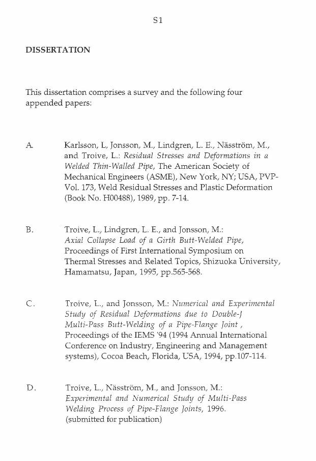
processes were made between 1880 and 1900. On the next page, in

Figure 1. the history of some important developments of welding

methods f r o m the 1880s and onwards are shown.

S4

1980

1970

1960

1950

1940

1930

1920

1910

1900

1890

1880

Welding fabrication of Saturn V space rockets.

Electron Beam, Ultrasonic, Laser Welding introduced.

Large scale research started on failures due to welding. War effort greatly advances use of welding in shipbuilding: Development of TIG, MIG, Other Welding Processes.

TIG (Tungsten Inter Gas), Hobart and Denver

First use of Metal Arc Welding in shipbuilding.

Covered Electrodes, O. Kjellberg.

Oxyacetylene Blowpipe, Le Chatelier. Melting Metal Electrode, Coffin. Resistance Welding, E. Thompson Carbon Arc Welding, N. Bernardo.

Figure 1. Part of the weld ing process history.

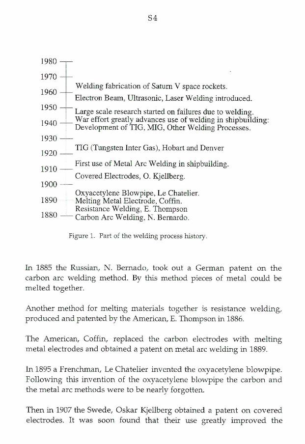
In 1885 the Russian, N . Bernado, took out a German patent on the

carbon arc welding method. By this method pieces of metal could be

melted together.

Another method for melting materials together is resistance welding,

produced and patented by the American, E. Thompson in 1886.

The American, Coff in , replaced the carbon electrodes w i t h melting

metal electrodes and obtained a patent on metal arc welding in 1889.

In 1895 a Frenchman, Le Chatelier invented the oxyacetylene blowpipe.

Following this invention of the oxyacetylene blowpipe the carbon and

the metal arc methods were to be nearly forgotten.

Then in 1907 the Swede, Oskar Kjellberg obtained a patent on covered

electrodes. It was soon found that their use greatly improved the

S5

properties of weld metals and allowed many new welding applications.

Today metal arc welding, using covered electrodes, is the most

commonly used welding process for manufacturing steel structures. The

oxyacetylene method is still widely used but in usually for non-critical

applications. The welding technologies since Kjellbergs patent of the

covered electrode have been developed to f u l f i l demands for welding

process automatizations.

I n the 1930s, the Americans, Hobart and Denver developed a method for

shielding the arc w i t h an inert gas f rom the atmosphere consisting of

nitrogen, oxygen and hydrogen. Their efforts led to the tungsten inert

gas (TIG) welding process. The electrode made of tungsten is not

consumed and by this method filler wire material can be used as needed.

This method was commercially used during the Second World War.

Later on the metal inert gas (MIG) was developed using continuously

fed consumable metal electrodes. Other types of welding-methods have

been developed during the last 40 years. Some of these are fr ic t ion

welding, plasma arc welding, electron beam welding and laser beam

welding. Today there are around 100 different types of welding process

variations available.

Dur ing the First World War, the metal arc welding process was used in

the shipbuilding industry. The method was limited to repairs and

welding of non-primary parts. But during the period of the Second

World War a large-scale production of ships was needed. Consequently

a faster joining process had to take place instead of the riveting

technique used before. Thereby, welded ships were built on a large scale

for the first time in history.

Brief history of computational weld simulations

It was shown that the experience and knowledge about ships welded

during the period of the Second World War were not sufficient, which

resulted in a large number of structural failures. Of the around 5000

merchant ships built in the USA during the Second World War, some

1000 structural failures due to welding were found. About twenty of

these ships were broken in two and sunk.

S6

A typical example of failure on welded ships during this period of time is

shown fn Figure 2, (from [6]). A similar failure happened as late as the

early 70s, Figure 3, (from [6]).

Figure 2. Figure 3. T-2 tanker Schenectady fractured Integrated T u g / Barge M . R. in 1943, [6]. Ingram fractured i n 1972, [6].

Because of these structural failures, research on a large scale started

after the war. Several organisations were founded at that time,

composed of major welding societies throughout the wor ld , e.g. The

International Institute of Welding, 1948. The areas for research were

then split into different branches, for example the metallurgy of

welding, fracture mechanics and thermal stresses. During the 50s and

60s much work was done on residual stresses and welding distortion. I n

[7], chapter 6, conclusions f r o m some of this work are summarised.

The prediction of residual stresses due to welding since the above

mentioned merchant ship's failures during the Second World War has

come to be very important for any types of constructions welded. I n

1949, Soete,[8] improved a method for measuring residual stresses,

called "centre hole dril l ing technique", developed by Mathar, 1934. This

method is still often used in industry. Due to the very expensive

procedure of first prototyping and thereafter experimentally evaluating

the magnitudes of stresses, the objective among researchers has been

(and still is) to investigate efficiently good numerical models for

analyzing the effects of welding on structures. The main problem has

S7

been to solve the theoretical models investigated before the advent of

computers during the 70s. Often simplified approaches and idealizations

had to be made to make i t possible to solve these types of problem e.g.

Okerblom [9].

The current strategy using computers for analyzing welds began during

the latter part of the 70s where the pioneers were Hibbit and Marcal [10]

using the finite element method(FEM) to solve these types of problem.

A t that time the performance of computers was not enough to solve fully

3D problems, which was why the geometric complexity had to be

reduced into 2D-models. Even today, when high speed performance

computers are available, that type of approach is still common due to

the fact that the researching area for the prediction of welding residual

stresses and deformations has been concentrated to even better simulate

and modulate the behaviours of the material in the immediate region of

the weld. The research area of welding simulations of today can be

divided into different branches which all attempt to improve the

numerical modelling of welding by use of FEM. In the next chapter, an

overview is given of the research activities in progress in the area of

simulation of welding using FEM.

Finite element simulation of welding, an overview

In comparison w i t h some other types of present mechanical simulations,

this current type of problem is very complex and unlinear due to the

strong dependence of the temperature history of the steel-material.

Consequently, an ordinary welding simulation is therefore divided into

several sub-steps by time-increments. A simulation then proceeds until

the time when room temperature is obtained. Even if today's computers

are used, several simplifications have to be made to receive reasonable

computer-times.

When material is melted or near melted in the region of the weld and

thereafter cooled rapidly, the microstructure w i l l be affected.

Depending on the steel-material, the material changes phase at certain

temperatures. When the temperature increases the micro-structure w i l l

change the phase to austenite. Depending on peak temperature reached,

S8

parts of the material has begun to melt (solidus-temperature) or is

totally melted (liquidus-temperature). Thereafter when cooling takes

form, the first phase formed is ferrite and then followed by bainite and

martensite. The decomposition of the latter mentioned phases, depends

on the cooling rate. Thereby, the residual state of micro-structure after

welding depends on the maximum temperature reached and the cooling

rate. I n other words, the micro-structure evolution of each point w i t h i n

the heat affected zone of the structure is strongly dependent of the

temperature history.

If we consider a ful ly coupled-thermo-mechanical simulation of

welding, the microstructure evolution prescribed above, w i l l affect both

the thermal and the mechanical fields, both of which are also affected by

each other. These effects are:

• Thermal and mechanical material properties w i l l be changed

due to microstructure evolution.

• Stresses and strains are increased caused, by volume changes

due to phase transformations.

• H igh strain rate and plastic strain produce heat.

• Stresses influence the phase-transformations.

A n outline of these couplings is given in Figure 4, below (from [11]).

Figure 4. Coupled thermo-mechanical analysis.

S9

Some of these couplings are dominant; others are of secondary types. I f

the weak couplings are found, this w i l l present possibilities for

simplifications which may be needed to receive a reasonable computer

time for weld simulations. Explanations of the Couplings, Comments

and Results according to Figure. 4, is shown i n Table 1.

R E M A R K C O M M E N T S / R E S U L T S

1 Microst ructure depends on thermal history. Phase Transformations - Dominant Coupl ing /

Experimental ly inc lud ing (3) or Numerica l ly by

L. E. Lindgren and A . Oddy, [12]

2 Thermal history is affected by latent heat due to phase transformations.

- Secondary C o u p l i n g / B. A . B. Andersson, [20]

3 Mechanical properties depend on micros t ruc ture evolu t ion .

Vo lume changes due to phase transformations.

Transformat ion Induced Plasticity.

- Dominant Coupl ing / Exper imental ly

or Numer ica l ly by: L . E. Lindgren and A . Oddy, [12]

- Dominant Coupl ing / Experimental ly inc lud ing (1)

or Numer ica l ly by: L . E. Lindgren and A . Oddy, [12]

- Dominant Coupl ing / Numer ica l ly by:

L. E. Lindgren and A . Oddy, [12] D. Dubois et al. [14]

J. B. Leblond et al. [15] C. T. Karlsson [18]

4 Stresses influence phase transformations. - Secondary Coupl ing / T. Inoue and Z. G. Wang [21]

B. L. Josefson [22]

5 Mechanical ly generated heat. - Secondary C o u p l i n g / Numer ica l ly by:

B. L. Josefson, [22] L. Karlsson, L. E. Lindgren [17]

6 The rma l expansion. - Dominant C o u p l i n g / Exper imental ly

or Numerica l ly by: L. E. Lindgren and A . Oddy, [12]

Table 1. Couplings i n Figure 4.

SIO

It can be seen f rom Table 1 that all the dominant couplings (1), (3) and(6)

have already been investigated, mainly by L. E. Lindgren and A Oddy,

[12]. The strangeness in [12] is that the coupling effects investigated are

all treated together. The problem investigated in [12], is a Satoh test

where microstructure evolution as wel l as temperature-dependence of

material properties were evaluated, simulating an experiment

performed in [13]. Good agreement was obtained. Their work is thereby

a first step towards integrating simulation of the microstructure

evolution into a finite element code. However, there is still a lot of work

remaining to complete an ordinary welding simulation w i t h the

microstructure evolution model integrated.

The effects of transformation plasticity (3) in welds i.e. when a stressed

body undergoing a phase transformation can exhibit plastic

deformations even if stresses are much lower than the yield l imi t , was

first analyzed by D. Dubois et al.[14] and later on by J. B. Leblond et al .

[15] using plain strain conditioned fe-models. The first 3D thermal stress

analysis including the transformation plasticity was performed by

A. Oddy [16]. Several simulations have since [16] been performed (e.g.

L. Karlsson and L. E, Lindgren [17], C. T. Karlsson [18] and L. Wikander

et al. [19]) analyzing the effects f rom the transformations plasticity on

the residual stresses by comparing w i t h experimental results.

The effect of latent heat due to phase transformations (2) was suggested

by B. A. B. Andersson in [20]. He implemented the latent heat by

increasing the magnitudes of the heat capacity in the interval between

the solidus and the liquidus temperatures. The magnitude in the middle

of the above mentioned interval was set to a value corresponding to the

latent heat. This method has been frequently used since [20], 1978.

The influence of the stresses on phase transformations, coupling (4), in

welding problems has been investigated by T. Inoue and Z. G. Wang [21]

and by B. L. Josefson [22]. That may be important when martensitic

transformation occurs.

The coupling (5) was studied by J. H . Argyris et al. [23]. They found that

the influence of the mechanical coupling (5) on the temperature field is

very weak. A couple of years later, also, the weakness of coupling (5)

S i l

was pointed out by B. L. Josefson [22]. Later on again the influence of (5)

on the temperature field was investigated by L. Karlsson and L. E.

Lindgren [17]. The conclusion f rom [17] was that the coupling (5) in the

heat equation must be negligible as the mechanical energies (5) are about

1/1000 of the thermal energies (6), see Figure 4. I t gives a maximum

calculated temperature difference between coupled and uncoupled

analysis, less then 1/100 of melting temperatures of metals.

Even if the outline shown in Figure 4 is numerically improved, the

transient temperature field i.e. the driving quantity, still has to be

determined efficiently by use of the finite element method, especially in

the region of the heat source. Due to the very high gradients which

occur near the heat source, a fine mesh is needed. On the other hand, to

reduce the computation complexity of the problem a coarser mesh has to

be used i n other parts of the structure. McDi l l [24] showed that by using

a developed graded element in the weld region instead of an ordinary

type of brick element, the number of freedom (DOF) w i l l be reduced

essentially w i t h no reduction in accuracy. To keep away f r o m a more

highly intensitive mesh along the whole weld line, i.e. only in the region

of the moving heat source that is needed, a dynamic mesh procedure

was developed by McDi l l [24], in combination w i t h the developed

graded element.

The "mixed-meshing" is another type of technique reducing the

computational complexity. By this method (developed and tested by

M . N ä s s t r ö m et al. [25]), brick elements are used in the region of the

weld and shell elements far f rom the weld. According to [25], i n the

interface between the two types of elements used, a geometrical

transformation algorithm by J. D Chieslar and A. Ghali [26] was

implemented.

To calculate the transient temperature field even better in and near the

region of the weld pool, in the future when very high performance

computers are available, the goal is to modulate the arc physics and

f lu id mechanics into finite element simulations of welding. A part of this

area of work, including analytical solutions of temperatures, velocities,

pressure as wel l as the geometry of the weld pool, is summariszed and

discussed in [27] by Y. Ueda and H . Murakawa.

S12

This overview given above, is a short illustration of the research

activities in the area of simulations of welding. This field of research is

also discussed and summarized in [28] by J. Goldak et al. and i n [29] by

B. L. Josefson.

Background

The residual deformations and the stress fields in jointed pipes due to

welding, have been investigated by many preivious workers. When

desigrüng a structure which consists of butt-welded pipes, it is of great

interest to know not only the future mechanics and thermal loads acting

on the joint but also the remaning fields of deformations and stresses

due to the welding process. For example, i n the process, offshore and

nuclear industry, butt-welding of pipes into piping systems is used fo r

transportation of several types of liquids. I t is wel l known that pipes are

very sensitive to stress-corrosion on the inner surface if tensile stresses

occur. Tensile residual stresses may also cause crack phenomena. On the

other hand, if too high compressive residual stresses are produced in the

pipe, the axial buckling load may be reduced.

Another common type of pipe joint in many applications is the pipe-

flange joint. The main advantage of this type of joint compared to the

above mentioned butt-welded joint is the much easier handling during

mounting and dismounting of parts in the system. It is also the best type

of joint when the two pipes to be connected are made of different

materials. The two pipes are usually connected by bolts through the

fixed flanges or via an extra loose flange that connects to the fixed or

loose flange on the other pipe. In both cases it is essential that the

contact surface of the flange that is fixed to the pipe is plane, so leakage

f rom the pipe is prevented. I f a pipe w i t h a distorted flange is mounted

using force to prevent any leakage, i.e. using the bolt-joint for reduction

of the gap between the two flanges, tensile-stresses may be induced,

which also means that the interface between the two pipes mounted w i l l

be sensitive to stress-corrosion. When manufacturing a pipe w i t h flange,

the flange is attached to the end of the pipe by a weld joint. Due to

welding induced thermal stresses both pipe and flange deform. H o w the

S13

flange is distorted (twisted) depends on the groove shape and the

welding sequence.

However, i t is easy to imagine the problem in ensuring a high

qualitative joint during a welding process. Therefore, the objective

among designers and researchers has been to develop numerical

methods for prediction of residual stresses and deformations. I n the

area of single-pass butt-welding of pipes, there exist several analytical

solutions for estimations of the residual stress field, e.g. R. H . Legatt

[30], and S. Vaidyanathan et al. [31]. These analytical solutions are based

on several assumptions made, such as rotational symmetry, elastic thin

shell theory and constant temperature dependence of material

properties. The analytical solutions in [30], and [31] were in [32]

compared w i t h experiments performed by Jonsson and Josef son. Fairly

good agreement between experiment and analytical solutions was

obtained. In [33] an additional analytical solution was developed by

Vaidyanathan et al., for prediction of residual stresses and deformations

in multi-pass butt-welded pipes. Different material properties in base

and fi l ler material is considered i n the model.

By using the finite element method instead of the above mentioned type

of analytical solutions, geometrical and material nonlinearities can be

accounted for. Since 3D-nonlinear FE-analyses of welded pipes are very

time-consuming, e.g. i n [34] by R. I . Karlsson and B. L. Josefson -about a

hundred CPU-hours were used on a IBM 3081D- , different types of

simplified approach has been employed in the welding simulations

performed. One type of simplification is by treating the pipe as a shell

(as i n paper A) or by the assumption of rotational symmetry. The latter

type of simplification is the most frequently used in the field of welding

simulations of pipes. Such analyses of single-pass butt-welded pipes

have been reported by e.g. E. F. Rybicki et al.[35], B. L. Josefson [36] and

C. T. Karlsson [18]. If we take a look at the simulations of multi-pass

butt-welding of pipes performed, often additional simplifications have

to be made due to the higher order of complexity of the problem

compared to a simulation of a single pass-weld. The latter type of

analyses has been investigated by e.g. E. F. Rybicki et al. [37, 38] and B. L.

Josef son [39].

S14

Simulations of buckling phenomena of thin walled pipes using F E M

have been reported several times before in scientific literature. In most

cases studied, different types of geometrical imperfections have been

accounted for investigating the influence of the axial load carrying

capacity for varying geometry of pipes. In the present paper B, the effect

of welding residual stresses in addition to the welding residual

deformations on the axial load carrying capacity is also investigated

using FEM in both simulation of welding and buckling. Similar studies

have been performed before by L. H ä f n e r [40] and in [41] by F. G.

Rammerstorfer and I . Skrna-Jakl. Instead of using FEM in the

calculation of the residual deformations and stresses due to welding,

they considered analytical solutions assuming rotational symmetry.

In the area for the simulation of multi-pass welding of pipe-flange joints

a simplified model using beam-ring-theory has been developed by B. L.

Josef son and L. Wikander [42]. The objective of this model is to estimate,

by a fast numerical analysis, the residual deformations of the flange

depending on the weld parameters used. I t was found in [42] that a

plastic material behavior of the r ing has to be implemented to improve

the model. Geometry as well as welding parameters used in [42] was

taken f r o m the experiment performed in paper C. This simplified model

has since [42] been further developed [43]. In paper C and D ,

respectively, simulations of multi-pass welding of pipe-flange joints has

been performed using FEM instead.

Present dissertation

Single-pass butt-welding of pipes and multi-pass welding of pip-flange

joints are simulated using the finite element method. Results obtained

f rom simulations are compared and verified w i t h corresponding

experimental quantities. Furthermore, simulations of axial loading of

thin-walled butt-welded pipes are performed, where the influence of

residual stresses and residual deformations on the axial load carrying

capacity are investigated.

S15

A brief description of the appended papers is given below.

In paper A, single-pass butt-welding of a

thin-walled pipe is simulated, where

residual deformations and residual stresses

are calculated. The temperature field

during and after welding unti l cooling is

calculated using an analytical solution. In

the mechanical part of simulation the finite

element method is used where the th in-

walled pipe considered is built up of shell

elements. The results of residual stresses

and radial shrinkage obtained f rom the simulation is compared w i t h

corresponding experimental quantities. The residual shrinkage was

measured using a cutting technique. Good agreement was obtained.

In paper B, an application of results

obtained f r o m additional simulations of

butt-welding of thin-walled pipes is

performed by turning the fields of residual

stress and residual deformations into a fe-

model for buclding analysis, investigating

the axial load carrying capacity for butt-

welded pipes. In this investigation two

butt-welded pipes w i t h different radius-to-thickness ratios (a/h), 106

and 53 respectively, are studied. The axial force applied versus axial

deformation of the welded pipe is compared w i t h corresponding

quantities for a perfect pipe and a pipe w i t h welding distortion

excluding welding residual stresses. The result gives an indication of

which of the individual welding effects, i.e. welding residual stresses or

distortions due to welding, have the greatest influence on the reduction

of the load carrying capacity for the two types of pipe geometry studied.

S16

I n paper C and D respectively, mu l t i ­

pass welding of two pipe-flange joints

considered are investigated both /% j numerically and experimentally. When / ff^-L • -r^

manufacturing pipe-flange joints, a I

flange is welded to one end of a pipe. f~xi -—\—

Consequently large residual stresses are ] 1 ^ [ ^ ^ ^ ^ ^ ^ " ^ ^ " y ^

induced and residual deformations as \ \ j\)\rJ_^~~--~-^

well . To avoid any risk of leakage \^éy J J

between two mounted pipes,

geometrical distortions (twisting) of the

flange w i l l be prevented. How the flange is distorted depends both on

the groove shape and the weld sequence used. However, to avoid f r o m

machine work after the welding process, the distortions have to be

minimized. In the two analyses performed, rotational symmetry is

assumed, for which reason only a cross section of pipe, flange and weld

material is included into fe-model. The supply of weld material is

simulated by using "born and die technique" and in the latter study

(paper D), the modelling of the contact between pipe and flange is

performed by using contact elements. In addition to the first pipe-flange

joint investigated in C, where only the residual distortion of the flange

was measured, a large amount of work has been devoted during D to

experimental verifications of results obtained after each weld pass by a

casting-technique developed. Measurement of the residual shrinkage of

the pipe is carried out by use of micrometer-screw in the opening

work , C, and by use of a coordinate-measuring machine in the latter

part of work, presented in paper D.

S17

SIMULATIONS

The simulations of butt-welding of thin-walled pipes, buckling of

welded pipes and multi-pass welding of pipe-flange joints performed in

appended papers are briefly described below.

Finite element models

In the simulations of welding performed, the finite element method

(FEM) was used both in the thermal and mechanical analysis, except for

the investigations of butt-welding of thin-walled pipes reported in

paper A and B, where the temperature field was calculated analytically

using a solution by Rosenthal. Futher details about the implementation

of this solution can be found in [44].

In paper A, residual stresses and diametrical deflections after

circumferential welding of a pipe were calculated using an in-house fe-

code STEPP [45]. The material was assumed to be thermo-elastoplastic

w i t h temperature-dependent mechanical material properties. In

addition to the material model used, the hardening modulus was set to

zero. Furthermore, due to the simplified solution used in the thermal

analysis (mentioned above), the thermal material properties were

constant. I n the fe-modelling of the pipe, only one half of the welded

pipe needed to be analyzed due to the symmetry. The analysed pipe was

divided into 448 four-node shell elements using 488 nodal points.The

supply of filler material into the groove was simulated by increasing the

element thickness in front of the moving heat source. The simulation

proceeded until room temperature was obtained using 89 time

increments for the welding and 25 time increments for the cooling phase.

In paper B, two butt-welded pipes w i t h different radius-to-thickness

ratios, 106 and 53 are studied numerically using the fe-code

NIKE3D [46]. The analytical solution for the temperature field used in

paper A was adopted into the current fe-code. The same material model

as wel l as the material properties as in paper A was also used.

S18

The welding simulations were performed in the same manner as in

paper A After the simulation of welding and cooling to room

temperature, axial loading was applied in the analysis unt i l buckling.

The axial loading was simulated by a moving rigid wa l l in contact w i t h

the end of the pipe. No friction between the end of the pipe and r igid

wal l was considered. The force versus axial deformation of the welded

pipe was compared w i t h corresponding quantities for a perfect pipe and

a pipe w i t h welding distortion excluding welding residual stresses. The

pipes investigated were both divided into 896 four-nodes shell elements

using 960 nodal points. Large deformations were accounted for in both

the welding simulation and the buckling simulation performed.

In Paper C and Paper D, respectively, deformations and stresses during

and after multi-pass welding of the pipe-flange joint are studied

numerically using an in house finite element code TEPP [47]. I n the

simulations performed, a simplified approach was employed, assuming

rotational symmetry. The assumption of rotational symmetry means

that only a cross section is studied, neglecting the heat f l o w in the

circumferential direction. In the simulation of the supply of weld

material for each weld pass, the so-called "born-die technique" was

used. I n this technique the cross-section of each weld pass is divided into

finite elements as wel l as the other parts of the structure, i.e. flange and

pipe. Initially before start of simulation the finite elements representing

the filler material are inactivated, i.e. an essential low stiffness is

assigned to these elements. When the supply of weld material is

simulated the current elements are activated (birth) which means that

the mechanical material parameters are changed to the original for the

weld material used. Furthermore, in the thermal analysis

thermodynamic coupling was not considered which is why only the

temperature field was coupled through the temperature-dependent

constitutive properties and the thermal strain. The thermal loading,

representing the energy f rom the mult i passes of welds supplied, are

applied as nodal heat inputs. The nodal heat input was constant

distributed over the cross-section area for each weld-pass. The material

was assumed to be thermo-elasto-plastic w i t h an isotropic hardening

behaviour. In the mechanical analysis large deformations were

accounted for. The type of finite element used in the thermal and

mechanical analysis was a four-node element. In the finite element

S19

model presented in paper C, 1476 elements and 1560 nodal points were

used. The size of the model analyzed in paper D, was 1150 elements

using 1263 nodal points.

Material Modelling

Owing to the type of material treated, different approaches and

simplifications have been employed in the modelling of the interactions

between temperatures, stresses and microstructures. All simulations

performed can be explained by Figure 5, shown below. When comparing

Figure 5 and Figure 4, one can see that several couplings are ignored or

replaced by quantities which are experimentally obtained. The effects of

the simplification depend on the type of material used and whether i t

undergoes phase transformations when heated or not. Details about

these effects are described below.

THERMAL FIELD

v

THERMAL PROPERTIES

EXPERIMENTS

MECHANICAL 1 MECHANICAL 1 FIELD PROPERTIES

Figure 5. S impl i f ied procedure for thermo-mechanical analysis.

The advantage of the simplifications performed is that a simulation can

be divided into two consecutive analyses, i.e. a thermal and a

mechanical analysis, and thereby decrease the computer time for

solving the problem essentially (see Figure 5). First a thermal analysis is

S20

performed. Then the temperature field obtained is used as input in a

subsequent mechanical analysis where displacements and stresses are

calculated. The thermal loads applied in the mechanical analysis are

given by the relations between temperature and thermal dilatation. The

temperature dependence of thermal dilatation as well as the rest of

mechanical and thermal material properties used, is experimentally

obtained based on computed temperatures or experimental data

available in literature. In this dissertation, volume changes due to

phase-transformations have not been treated at all in any of the

appended papers (A to D).

The butt-welded thin-walled pipe investigated in paper A, was f i rs t

studied numerically by L.E. Lindgren and L. Karlsson [44], including the

influence of volume change due to phase-transformations. In that type

of material model, the strains which are induced by the phase

transformations are added to the thermal strains of the material i.e.

called thermal dilatation, which give the total amount of thermal strains

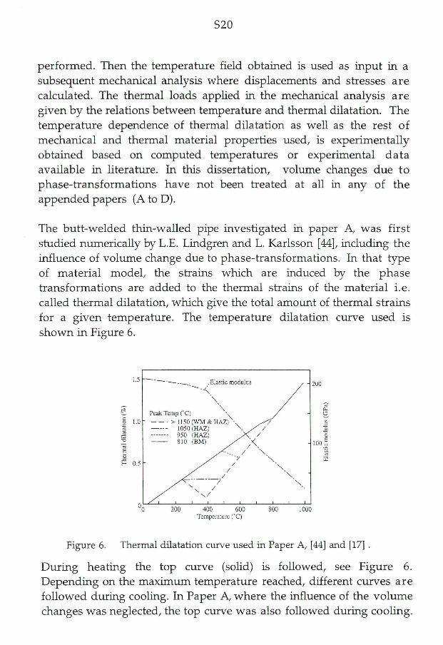
for a given temperature. The temperature dilatation curve used is

shown in Figure 6.

Temperature (°C)

Figure 6. Thermal dilatation curve used i n Paper A , [44] and [17] .

During heating the top curve (solid) is followed, see Figure 6.

Depending on the maximum temperature reached, different curves are

fol lowed during cooling. In Paper A, where the influence of the volume

changes was neglected, the top curve was also followed during cooling.

S21

It was found in [44] that very high compressive hoop-residual stresses

are obtained in the weld centre on the outer surface of pipe if volume

changes due to phase-transformations are accounted for. Later on an

additional investigation [17] was performed by also including the

transformation plasticity [12] into the material model. Still there was a

difference between the experimental and the numerical results obtained

in the centre of weld. If comparing the results evaluated by use of the

above mentioned material models w i t h the experimentally obtained

residual hoop stress, good agreement is obtained only if the volume

changes are ignored (as in Paper A) . In all cases mentioned above

including paper A, an ideal-elasto-plastic material model was used.

During the same period of time as [44], a fu l ly three-dimensional finite

element analysis of a single-pass butt-welded pipe was investigated by

R. I . Karlsson and B. L. Josefson reported in [34]. The same type of

material model was considered as in [44], where the volume changes due

to phase-transformations were accounted for (without transformation

plasticity). They also notified results of compressive hoop stresses in the

weld. I t was concluded that it is much easier to investigate and develop

different material models by using a simple axi-symmetric model

compared w i t h an extremely time-consuming three-dimensional

analysis.

That type of investigation was thereafter started by C. T. Karlsson

reported in [18]. He studied the effects of using different material models

in the simulation of a single-pass butt-welded pipe in a rotational

symmetric fe-model. Similar results were obtained there also. It was

found in [18] that the best agreements w i t h respect to the residual hoop

stress were reached when using the simplest material-model, i.e. when

volume changes are not accounted for.

S22

S23

EXPERIMENTS

Temperatures

In order to determine the arc efficiency r\, temperatures were measured

at different distances f r o m the weld. In paper A, B and D, temperatures

were measured by use of N i - C r N i thermocouples, which were spot

welded to the pipes.

Dilatation test

If considering a temperature history dependence of the material

properties, several approaches have to be employed to reduce the

number of experiments. That means that when the material behaviours

are obtained experimentally, only a low number of peak temperatures

and cooling rates can be tested. During experiments specimens are also

unloaded which ignore any effects f rom the stresses on the phase

transformations, even if it is a weak coupling.

When preparing for a material test, the first step is to perform a welding

experiment (the same or similar welding procedure that w i l l be

simulated later). In that experiment temperatures are recorded at some

few points near the weld. The peak temperatures as wel l as the time for

cooling f r o m 800°C to 500°C are registered. These temperature are

thereafter used as input into the dilatation-test where the dimensional

changes are recorded during a heating and a cooling phase of a small

sample made of the steel material tested.

Deformations

In paper A, C and D, residual diametrical shrinkage after welding was

measured using different techniques.

In paper A, a cutting procedure was used. Using this technique, the

diameter of a welded pipe is measured at several points, which are

S24

marked up carefully. Thereafter, the pipe is cut parallel to the weld line

at a definite distance f rom the weld. That distance should be chosen so

that part of the pipe which does not contain the weld is free f r o m plastic

strains. The diameter is once again measured at the same positions as

before the cutting. Thereby, the diametrical change due to welding is

obtained. The diameter was measured by use of a micrometer-screw.

In paper C, the residual deformations due to multi-pass welding were

determined on both the pipe and the flange. On the outer surface of the

pipe and the flange, the diameter change was measured in four

circumferential positions (every 45 degrees). Al l measurements were

performed before and after welding at the same points, which were

permanently marked before the start of the experiment. The difference

between the diameters measured gave the desired quantity. On the

flange the twisting distortions were measured w i t h a dial indicator at

every 45 degrees.

In paper D, the change in geometry of the four pipes considered, i.e. due

to multi-pass welding, was measured by use of a coordinate-measuring

machine. Measurements were performed before and after welding at

about 2000 points each. The experimentally obtained results presented

in paper D are the circumferential mean value of the radial shrinkage.

In additional to the radial shrinkage of the pipe, the flange deflections

have also been investigated experimentally. I t was found in paper C

that a more sophisticated measuring method for determination of the

flange distortions has to be developed. The objective was also to detect

the flange distortion during the welding process. A special casting

technique was developed.

In this technique a special dental foam PROVTL [48], is used as a cast

compound. Measurements of the twisting angle of the flange were

carried out before the start of the welding procedure, after each weld

pass and finally when the welded pipe flange joint had cooled to room

temperature. In these measurements a flat smooth ground circum­

ferential plate was used as a reference plane. This plate has three sharp

spikes located symmetrically. At the time for measurement, three wel l

sized pieces of the dental foam were symmetrically placed on the plate

which thereafter was placed wi th the spikes positioned on the end of the

S25

pipe. I n this measuring procedure the dental foam is pressed between

the flange and the reference plate, see Figure 7 and Figure 8.

Figure 7. Figure 8.

Detection of flange distortions du r ing Cross-section of measurement setup fo r

w e l d i n g process by casting technique. detection of twisting-angle 6 of flange.

The three spikes as wel l as the dental foam were placed in the same position i n all the casts performed. Assuming rotational symmetry, the twist ing angle of the flange can be obtained by evaluating the mean profi le of these three pieces casted.

Thermal shrinkage of specimen

When making a dental foam cast of the flange during experiment, the

temperature was around 300°C and the specimen were thereby cured at

a high temperature. Consequently the cast compound shrinks during

cooling down to room temperature. The effects of the shrinking of

specimens are assumed to have no influence on the determination of the

twist ing angle (J). But when we study the axial translations 8Z

(z'-direction, see Figure 9) of a point located on the flange, the measured

data have to be compensated. Here follows a description of the model

that has been used to establish the magnitudes of shrinkage.

S26

The thickness of the casted blocks was measured (described in detail i n

paper D) at several points each. The results obtained f rom each block

casted were three series of data giving three straight lines including

angles of inclinations and correlation factors. To receive only one piece

of data for each block casted, a weighted mean value was calculated by

using the correlation factors. Thereby inaccurate measuring data were

filtered. Finally the twisting of the flange was determined by taking the

mean value (mentioned above) of the results obtained f rom the three

blocks casted.

Figure 9. Mode l fo r establishment of shrinkage magnitudes of specimens.

A local r'-z'-coordinate system was used in the linearization of the

measuring data (see Figure 9). The z'-axis lies along the outer surface of

pipe parallel to the global axial direction starting at the surface of

fixture. The local radial axis r', starts at the outer surface of the pipe.

When placing the equations for the straight lines evaluated in the local

coordinate system, a constant term, K j , is obtained i.e. where each

function crosses the z'-axis. Each straight line is an assumed fictitious

flange, where the axial position (fictitious contact point) of the flange is

to be the same value as for the constant term, K i ; in the equation, see

Figure 9. Due to the fact that the contact point between flange and pipe

S27

is able to move or translate in z'-axial direction (even if i t is tack-

welded) unt i l the first pass of weld is brought to an end, the constant

term, Kir in equation is therefore assumed to be fixed through all

measurements except the first one K 0 , obtained before the start of

welding and, K n , obtained at room temperature (when the f inal pass of

weld is finished). Thereby, i t would be possible to estimate the thermal

shrinkage of each specimen by using the constant term, K n , of the

equation evaluated f rom the f inal measuring data as a reference, K, . e f ,

obtained at room temperature.

It has been seen f rom the experimental results obtained that the term K,

is really not fixed when the flange is heated. In Figure 10, the variation

of K is shown f r o m experiment B.

K ref

14,20

14,10

1 4,00

1 3,90

1 3,80

1 3,70

13,60

13,50

1 3,40

1 3,30

1 3,20

» Ki

1 o 11 0 1 2 3 4 5 6 7 8 E

W e l d p a s s No

Figure 10. Coordinate of f ic t ive contact point K ; between flange and pipe i n [mm] .

The fluctuation of K can probably be explained by the accuracy of the

measuring data, varying temperatures and varying casting times i.e.

heating up when curing. The error bars shown in Figure 10 are the

variations of data obtained f rom each measurement. In the

compensation for shrinkage thermal expansions of the end of pipe i.e.

f r o m position of flange to end of pipe, would also be included. The

S28

magnitude for the thermal expansion is estimated to be 0.05 m m and in

comparison to the shrinkage of the plastic blocks casted, which are

around 0.3 mm (see Figure 10), the thermal expansion is negligible and

therefore not compensated for in the model.

In Figure 11, the z-translation 5Z of one point is studied during

experiment B. The point is located at the radius r=69 mm on the outer

surface of the flange (negative z-direction). One can see f rom Figure 11,

the difference in results obtained if compensation for thermal shrmking

of the casted blocks is accounted for or not.

1,5

CT> CD 1 J

E 0,5 E

cd o r j

CD Ü J _ Q-

W T3

NJ

•0,5

•FEM

o Compensated

o No compensation

0 2 0 0 0 4 0 0 0 6000 8000 10000 1 2 0 0 0 Time [sec]

Figure 11. Comparison between results obtained f r o m experiment B w i t h or w i thou t compensation for thermal shrinkage of the plastic blocks cast.

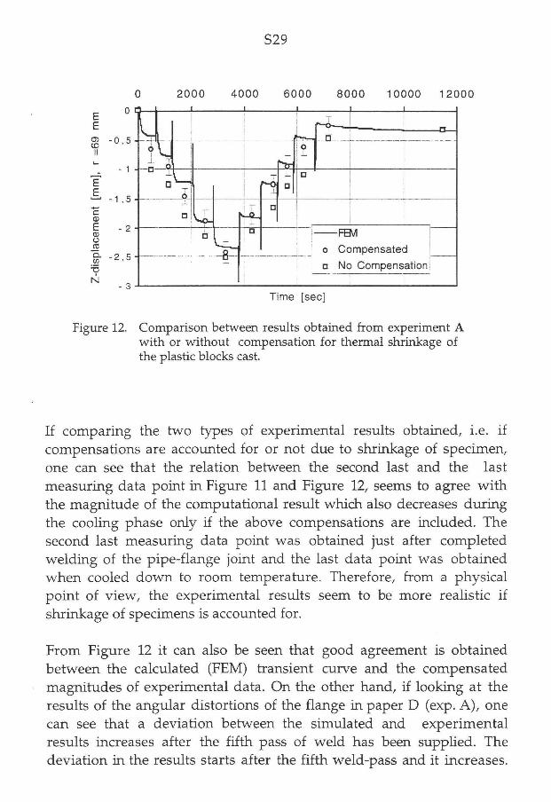
I n Figure 12 results f r o m experiment A are shown. The evaluation of the

shrinkage magnitudes in experiment A is performed in the same manner as for experiment B.

S29

2 0 0 0

E E

æ -0 ,5

E

•1,5

c cu E - 2 cu o CL . p rz

T3

N

4000

i

6 0 0 0

i

8 0 0 0 10000 1 2 0 0 0

ti

r-oi

-FEM

o Compensated

o No Compensation

Time [sec]

Figure 12. Comparison between results obtained f r o m experiment A w i t h or w i t h o u t compensation for thermal shrinkage of the plastic blocks cast.

If comparing the two types of experimental results obtained, i.e. i f

compensations are accounted for or not due to shrinkage of specimen,

one can see that the relation between the second last and the last

measuring data point in Figure 11 and Figure 12, seems to agree w i t h

the magnitude of the computational result which also decreases during

the cooling phase only if the above compensations are included. The

second last measuring data point was obtained just after completed

welding of the pipe-flange joint and the last data point was obtained

when cooled down to room temperature. Therefore, f rom a physical

point of view, the experimental results seem to be more realistic if

shrinkage of specimens is accounted for.

From Figure 12 i t can also be seen that good agreement is obtained

between the calculated (FEM) transient curve and the compensated

magnitudes of experimental data. On the other hand, if looking at the

results of the angular distortions of the flange in paper D (exp. A ) , one

can see that a deviation between the simulated and experimental

results increases after the f i f t h pass of weld has been supplied. The

deviation i n the results starts after the f i f t h weld-pass and i t increases.

S30

The difference in the angle distortion of the flange is probably due to

deviation of the radial deflection of the end of the pipe. From the

experiment the radial expansion of the end of the pipe was found to be

0.8 m m in comparison wi th 0.2 mm in the simulation. Due to the fact

that the flange is fixed to the pipe, the agreement of the latter results

show that the radial deflection of the end of the pipe is the cause of the

above mentioned angle deviation.

S31

DISCUSSION AND FUTURE DEVELOPMENTS

Different finite element models for welding simulations of welded pipes

were evaluated in paper A to D. The simulations performed have been

treated in different ways using e.g. shell element, assumption of

rotational symmetry or simplified material models. Al l these types of

numerical simplifications made are of two different types:

• Reduction in number of degrees of freedom (DOF).

• Neglecting couplings between the field of microstructure evolution,

thermal and stress fields.

In general, in order to receive reasonable computer time for a typical

welding simulation, using today's ordinary work-station, simplified

approaches have to be employed. Both of the two types of

simplifications mentioned above aim to reduce the computational

complexity. However, the simplifications and the approaches made still

have to be well-balanced in a physical sense.

However, do we know when the limit is reached for the simplifications

made? Results obtained f rom simulations are usually compared w i t h

corresponding experimental quantities to ensure the correctness in a

simplified fe-model. We know that this current type of problem is

strongly dependent of the temperature history and if any of the input

data to a verified fe-model is changed, results may not be reliable any

longer.

If studying the use of the finite element method in industry, it has come

to be very frequently used as a tool for reduction of prototypes

produced. Often, the problems solved in industry are of the nature

which gives opportunities for making changes in input data and thereby

also possibilities for optimizations.

The objective for the research in the area of weld simulation is to

improve and develop the fe-modelling of welding to meet the demand

f r o m industry in the near future. As we can see today, the experience of

S32

welding operators is lost when they are replaced by robots.

The consequence w i l l be that designers have to take the decisions

instead. Numerical simulations of welding w i l l therefore become more

and more useful.

Future research should be directed towards improvement of the

numerical modelling of the micro structure evolutions that have a

pronounced effect on the residual state after welding. The goal w o u l d be

that only the chemical compositions and mechanical material properties

at room temperature are needed as material input data. Parallel to that

work also, results obtained f rom simulations are to be verified. The

neutron diffraction method is the only method for measuring strains and

stresses in the interior of a material [2, 3]. This method would be an

important part of that future work.

Also future research activity on different types of boundary conditions is

needed, especially in the contact between the welding fixture and the

welded structure and also the contact which occurs between two parts

before jointed.

S33

REFERENCES

[1 ] Karlsson, L, Jonsson, M . , Lindgren, L. E., Näss t röm, M . ,

and Troive, L. : Residual Stresses and Deformations in a

Welded Thin-Walled Pipe, The American Society of

Mechanical Engineers (ASME), New York, NY, USA, PVP-

Vol. 173, Weld Residual Stresses and Plastic Deformation

(Book No. H00488), 1989, pp. 7-14.

[2 ] Troive, L., Karlsson, L., Näsström, M . , Webster, P. J., and

Low, K. S.:Finite element simulations of the bending of a flat

plate to a U-shaped beam cross-section and the welding to a

rectangular hollow cross-section and neutron diffraction

determination of residual stresses. Proceeding of the 2nd

International Conference on Trends i n Welding Research,

American Society of Metals, Materials Park, Ohio, USA,

pp. 107-111,1989

[3 ] Karlsson, L., Näss t röm, M . , Troive, L., Webster, P. J., and

Low, K. S.:Residual stresses and deformations in an Inconel

welded component.

[4] Hicks, J. C : Welded joint design, Granada Publishing, London, UK, 1979.

[5 ] Encyclopedia of Materials Science and Engineerings, Editor-

in-Chief: Bever, I . , Michael, B., MISBN 0-08-022158-0.

[6] Masubuchi, K.: Analysis of Welded Structures,

Pergamon Press 1980, ISBN 0-08-022714-7.

[7 ] AWS, Welding handbook, Vol. 26, pp. 519-529,1976.

[8] Soete, W.,: Measurement and relaxation of residual stresses,

Welding Journal, Vol . 28, pp. 354-364,1949.

S34

[9] Okerblom, N . O.: The Calculations of Deformations of

Welded Structures, London, Her Majesty's Stationery

Office, 1958.

[10] Hibbit , H . D., and Marcal, P. V.: Numerical Thermo-

Mechanical Model for the Welding and Subsequent Loading

of a Fabricated Structure, Comp. & Struct., Vol . 3,

pp. 1145-1174,1975.

[11] Lindgren, L. E.; Deformations and Stresses in Butt-Welding of

Plates, Ph.D. Thesis, Luleå University of Technology, Sweden,

1985.

[12] Lingren, L. E., and Oddy, A.S.: Toolbox for computing phase

transformations and material properties of hypoeutectoid

steels in Satoh test, Thermal Stresses '95, Hamamatsu, Japan,

June 5-7, pp. 517-520,1995.

[13] Jones, W. K. C , and Alberry, P. J. A.: A model for stress

accumulation of steel during welding, Int. conf on residual

stresses in welded construction and their effects, The Welding

Institute, London, England, p. 15, 1977.

[14] Dubois, D., Devauz, J., and Leblond, J. B.: Numerical

Simulation of Welding Operation: Calculation of Residual

Stresses and Hydrogen Diffusion, F i f th International

Conference on Pressure Vessel Technology, San Francisco,

Vol . 11, pp. 1210-1239.1984.

[15] Leblond, J. B., Devaux, J., and Devaux, J. C.-.Mathematical

Modelling of Transformation Plasticity in Steels I: Case of

Ideal-Plastic Phases, International J. of Plasticity, Vo l . 5,

1989, pp. 551-572.

[16] Oddy, A. S.: Three-Dimensional Finite Deformation,

Thermal-Elasto-Plastic Finite Element analysis, Ph.D. Thesis,

Carleton University, Ottawa, Canada, 1987.

S35

Karlsson, L., and Lindgren, L. E.:Combined Heat and

Stress-Strain Calculations, The Minerals, Metals &

Materials Society, pp. 187-202, 1991.

Karlsson, C. T.-.Finite element analysis of temperatures and

stresses in a single-pass butt-welded pipe — influence of mech

dencity and material modelling, Engineering Computation,

Vol . 6, No 2,1989.

Wikander, L., Karlsson, L. , Nässt röm, M . , and Webster, P.:

Finite element simulation and measurement of welding

residual stresses, Model l ing Simul. Mater. Sei. Eng,

Vol . 2, pp. 845-864,1994.

Andersson, B. A . B.:Thermal stresses in a submerged-arc-

welding joint considering phase transformations, ASME

Journal of Engineering Materials and Technology,

Vol . 100, pp. 356-362, 1978.

Inoue, T., and Wang, Z. G.:High-temperature behaviour of

steel with phase transformation and the simulation of

queching and welding processes, Mechanical Behaviour of

Materials - IV, Proceedings of the Fourth International

Conference, Stockholm, 1983.

Josefson, B. ~L.-.Effects of transformations plasticity on

welding residual-stress fields in thin-walled pipes and thin

plates, Material Science and Technology,

Vol . 1, pp. 904-908,1985.

Argyris, J. H . , Szimmat, J., and Will iam, K. J.: Computional

aspects of welding stress analysis, Computer Methods i n

Applied Mechanics and Engineerings,

Vol. 33, pp. 635-666, 1982.

M c D i l l , J. M . J.: An Adaptive Mesh-Management Algorithm

for Three-Dimensional Finite Element nalysis, Ph.D. Thesis,

Carleton University, Ottawa, Canada, 1988.

S36

Näss t röm, M . , Wikander, L., Karlsson, L., Lindgren, L. E., and

Goldak, J.: Combined 3-D and shell modelling of welding,

Proceeding of I U T A M Symposium on the Mechanical Effects

of Welding, Luleå, Sweden, 1991, Springer Verlag,

Heidelberg, Germany, pp. 197-206,1992.

Chieslar, J. D., and Ghali, A.: Solid to Shell element

Geometric Transformation, Computers & Structures,

Vol . 25, No. 3, pp. 451-455,1987.

Ueda, Y., and Murakawa, H . : Application of Computer

and Numerical Analysis Techniques in Welding Research,

Trans, of JWRL Vol. 13. No. 2, pp. 337-346, 1984.

Goldak, J., Oddy, A., Gu, A., Ma, W., Mashaie, A. , and

Hughes, E.: Coupling Heat Transfer, Microstructure

Evolution and Thermal Stress Analysis in Weld Mechanics,

Proceedings for I U T A M Symposium on the Mechanical

Effects of Welding, Luleå, Sweden, June 10-14, Springer

Verlag, Heidelberg, Germany, pp. 1-30, 1992.

Josefson, B. L.: Prediction of residual stresses and distortions

i n welded structures, ASME Journal of Offshore Mechanics

and Arctic Engineering, Vol. 115, pp. 52-57, 1993.

Legatt, R. H . : Residual Stresses at Circumferential Welds

in Pipes, The Welding Institute Research Bulletin,

Vol. 23, pp. 181-188,1982.

Vaidyanathan, S., Todaro, A. F., and Finne, L:

Residual Stresses Due to Circumferential Welds,

ASME, Journal of Engineering Materials and Technology,

Vol. 95, pp. 233-237,1973.

Jonsson, M . , and Josefson B. L.: Experimentally Determined

Transient and Residual Stresses in a Butt-Welded Pipe,

Journal of Strain Analysis, Vol. 23, No. 1, pp. 25-31, 1988.

S37

[33] Vaidyanathan, S., Weiss, H . , and Finnie, L:

A Further Study of Residual Stresses in Circumferential

Welds, ASME, Journal of Engineering Materials and

Technology,Vol. 95, pp. 238-242,1973.

[34] Karlsson, R. L, and Josefson, B. L.:Three-dimensional finite

dement analysis of temperatures and stresses in a single-pass

butt-welded pipe, ASME Journal of Pressure Vessel

Technology, Vol. 112, pp. 76-84,1990.

[35] Rybicki, E. F., Schmueser, D. W., Stonesifer, R. B,

Groom, J. J., and Mishier H . B.:A Finite Element

Model of Residual Stresses in Girth-Butt Welded Pipes,

Presentated at the 1977 ASME W A M , Numerical Modeling of

Manufacturing Processes, PVP-PB-025, pp. 1-18. 1977.

[36] Josefson, B. L./.Residual Stresses and Their Redistribution

During Annealing of a Girth-Butt Welded Thin-Walled pipe,

ASME, Journal of Pressure Vessel Technology,

Vol . 104, pp. 245-250,1982.

[37] Rybicki E. F., Stonesifer, R. B., Groom, J. J., and

Mishler, H . W.: A Finite-Element Model for Residual Stresses

and Deflections in Girth-Butt Welded Pipes, ASME Journal of

Pressure Vessel Technology, Vol . 100, pp. 256-262,1978.

[38] Rybicki E. F., and Stonesifer, R. B.: Computation of Residual

Stresses Due to Multipass Welds in Piping Systems, ASME

Journal of Pressure Vessel Technology,

Vol . 101, pp. 149-154, 1979.

[39] Josefson, B. L., and Karlsson, C. T.\FE-calculated Stresses in

a Multi-pass Butt-Welded Pipe - A Simplified Approach,

International Journal of Pressure Vessel & Piping,

Vol . 38, pp. 227-243,1989.

S38

Rammerstorfer, F. G., and Skrna-Jakl, l.:The influence of

welding stresses and distortions on the stabillity of shell of

revolution, Proceeding of I U T A M Symposium on the

Mechanical Effects of Welding, Luleå, Sweden, 1991,

Springer Verlag, Heidelberg, Germany, pp. 197-206, 1992.

H ä f n e r . L.:Einfluß einer Rundschweißnaht auf die Stabilität

und Traglast des axialbelasteten Kreiszylinders,

Doctoral Thesis, Univ. of Stuttgart, FRG, 1982.

Josefson, B. J., Wikander L., Hederstiema, J., and

Johansson, F.-.Welding residual distortions in

Ring-Stiffened Pipes, 14th International Conference on

Offshore Mechanics and Arctic Engineering (OMAE 95),

Copenhagen, Denmark, 1995.

Wikander, ^.-.Efficient thermomechanical modelling of

welding, Ph.D. Thesis, Luleå University of Technology,

Sweden, 1996.

Lindgren, L. E., and Karlsson, L.:

Deformations and Stresses in Welding of Shell Structures,

International Journal for Numerical Methods i n Engineering,

Vo l 25., pp. 635-655, 1988.

STEPP: Shell Thermo Elasto Plastic Program, Lindgren, L. E.,

Div . of Computer Aided Design, Luleå University of

Technology, Sweden.

NIKE 3D: A Nonlinear, Implicit , Three-Dimensional

Finite Element Code for Solid and Structural Mechanics,

Hallquist, J.O., University of California, Lawrence Livermore

National Laboratory, Rept. UCID-18822, 1990.

TEPP: Thermo Elasto Plastic Program, Lindgren, L. E., Div . of

Computer Aided Design, Luleå University of Technology,

Sweden.

S39

PROVIL, P-soft, Bayer Dental, D-51368 Leverkusen,

D I N 13913-Al, ISO 4823, Type 0.

S40

Paper A

A l

The American Society of Mechanical Engineers

Reprinted From PVP - Vo l . 173, Weld Residual S t r e s s e s and Plastic

Deformation Edi tors: E. Rybicki , M. Shirator i , G . E. O Widera, and T. Miyoshi

Book No. H00488 - 1989

RESIDUAL STRESSES AND DEFORMATIONS IN A WELDED THIN-WALLED PIPE

L. Kar lsson , Ni. J o n s s o n , L. E. L indgren, M. Nasst rom, and L. Troive Depar tmen t of Mechan ica l Engineer ing

Lulea Universi ty o f T e c h n o l o g y Lulea, S w e d e n

ABSTRACT

Deformations and stresses during butt-welding of a pipe are calculated as well as the residual deformations and stresses. The temperature field during welding is calculated using an analytical solution. The deformations and stresses are calculated by use of the finite element method. A thermo-elastoplastic material model is used. Special attention is paid to the influence of the volume changes due to phase transformations on the deformations (radial shrinkage) and the residual stresses. The calculated radial shrinkage and residual stresses are compared to experimental values. Good agreement was obtained.

INTRODUCTION

In earlier work conceming simulations of butt-welding of pipes mostly axisymmetric conditions have been assumed, see [1] and [2]-[6]. Recently three-dimensional simulations have been performed, see [7] and [8]. For a pipe with a thickness much smaller than its radius it is possible to reduce the size of the problem by modelling the pipe with shell elements.

Deformations and stresses during bun-welding and subsequent cooling of the pipe in Figure 1 are calculated. The residual stresses and the radial shrinkage of the pipe are compared to experimental results. For the temperature calculation during welding the analytical solution in [9] is used also in this study. The finite element method (FEM) is used in the calculation of deformations and stresses. In these calculations the shell element according to [9] is used. This element is based on the shell element according to Hughes and Liu, [10], and the coding of it in NIKE3D, [11]. The material was assumed to be thermo-elastoplastic. The volume increase due to phase transformations during cooling is not accounted for in the simulations presented in this paper for reasons given below (under THEORETICAL ANALYSIS).

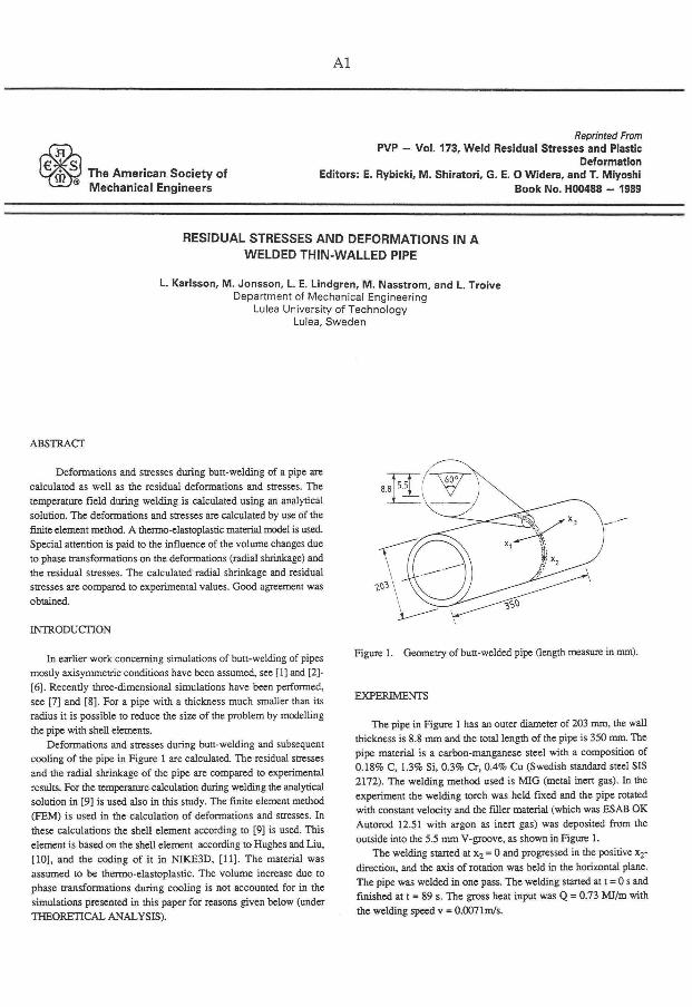
Figure 1. Geometry of butt-welded pipe (length measure in mm).

EXPERIMENTS

The pipe in Figure 1 has an outer diameter of 203 mm, the wall thickness is 8.8 mm and the total length of the pipe is 350 mm. The pipe material is a carbon-manganese steel with a composition of 0.18% C, 1.3% Si, 0.3% Cr, 0.4% Cu (Swedish standard steel SIS 2172). The welding method used is MIG (metal inert gas). In the experiment the welding torch was held fixed and the pipe rotated with constant velocity and the filler material (which was ESAB OK Autorod 12.51 with argon as inert gas) was deposited from the outside into the 5.5 mm V-groove, as shown in Figure 1.

The welding started at x 2 = 0 and progressed in the positive x2-direction, and the axis of rotation was held in the horizontal plane. The pipe was welded in one pass. The welding started at t = 0 s and finished at t = 89 s. The gross heat input was Q = 0.73 MJ/m with the welding speed v = 0.007 lm/s.

A2

In the investigation of the diametrical shrinkage the pipe was cut

parallel to the weld line at a definite distance from the weld. This

distance was chosen so that the part of the pipe which does not

contain the weld is free from plastic strain. The diametrical change

due to this cutting was measured. The pipes were cut apart with a

cold saw at x t = 13 mm and x_ = -13 mm. The saw was cooled with

cutting fluid and the rate of speed was low in order to minimize

introduction of new stresses. The diameter change was measured on

both sides of the weld (positive and negative Xj-values.see Figure 1)

to see if the shrinkage was symmetric with respect to the centre plane

(x! = 0). The diametrical residual shrinkage was evaluated in three

circumferential positions (cb = 0°,60° and 120°) and twentyfive axial

positions (from 15 to 170 mm away from the weld centre) on each

side of the weld. The diameter was measured with a micrometer

screw. The experimental procedure was the same as in [12].

The measured residual stresses are taken from [13].

THEORETICAL ANALYSIS

The analytical solution for the heat flow due to a point heat

source in an infinite homogeneous body with constant thermal properties can be used to construct solutions for a wide range of

problems [14]. The most well-known solutions are Rosenthal's solutions for a moving line/point heat source in a thin/thick infinite

plate. The thin plate solution is based on a heat source with uniform strength along a line through the thickness of the plate. The

temperature field due to this hne heat source can be applied to a pipe if the radius of the pipe is much larger than its thickness and the temperature is assumed to be constant through the thickness of the

pipe. Further details about the implementation of this solution can be found in [9]. Quite good agreement between calculated and measured temperatures is reported in [9].

The finite element method is used in the mechanical analysis. Constant temperature is used in each of the finite elements. This is consistent with the linear variation of the displacements within an

element. Because of symmetry only one half of the pipe in Figure 1 need be analysed (x^O.). The half pipe was divided into 448 four-

node shell elements (as those presented above) using 488 nodal

points, see Figure 2. A three-point Lobatto quadrature rule was used for the numerical integration in the thickness direction. The elements

closest to the line of symmetry (weld centre line) had the width 3.2

mm. These elements were given a thickness of 6.0 mm in front of the moving arc in order to account for the geometry of the groove

and 8.8 mm behind the arc. The mechanical analysis was performed

for times t = 0 to t = 14000 s using 89 time (load) increments for the welding and 25 time (load) increments for the cooling.

t i v

Figure 2. FE-mesh of half analysed pipe

The material was assumed to be thermo-elastoplastic with

temperature-dependent mechanical material properties . Von Mises

yield condition with the associated flow rule was used. The

hardening modulus is as in [9] set to zero in this study for the reason

that no good experimental values were available. Volume changes

due to phase transformations were accounted for in [9] by use of the

thermal dilatation E T which is given in Figure 3. These values were

in [9] taken from [7]. In this study the solid curve in the dilatation

diagram, Figure 3, was followed both during heating and cooling.

TEMPERATURE l°C]

Figure 3. Thermal dilatation eT and modulus of elasticity E for the

steel used:weld metal (WM), heat affected zone (HAZ), base metal (BM)

The temperature dependence of the modulus of elasticity E is also

given in Figure 3. The temperature dependences of Poisson's ratio v

and the yield stress o y are shown in Figure 4. All material points

(integration points) follow the solid curve for the yield stress in

Figure 4 during heating and cooling. At high temperatures the yield

stress is assigned low values varying from 20 MPa at 1000° C to 10

MPa at the melting temperature.

A3

PEAK TEMP C C )

»1150 (WM & HAZ) 1050 (HAZ)

0 200 400 600 800 1000

TEMPERATURE (°C)

Figure 4. Yield stress c y and Poisson's ratio v as functions of

temperature:weld metal (WM), heat affected zone (HAZ), base metal (BM)

The fact that the solid curves for £ T and o y are followed in Figure

3 and Figure 4 .respectively, implies that the influence of volume

changes due to phase transformations are not considered. It is clear

from the experimental values of eT that a relatively large volume increase occurs during the later part of cooling. This causes negative residual hoop stress at the outer surface at Xj=0 in the calculations. The measured residual hoop stress at this location was tensile (about 150MPa). The influence on the stresses of this volume change may partly be annihilated by the additional plastic strains which are believed to be formed due to the so-called transformation plasticity effects. As we do not have experimental data to include the transformation plasticity it is of interest to investigate a case where these volume changes are not accounted for. Thus we can see how important the volume changes due to phase transformation are for the residual states.

RESULTS

The measured change in diameter is shown in Figure 5a for three different angular locations and for both negative and positive values of the X]-coordinate. In Figure 5b the corresponding calculated values are shown.

In Figure 6 calculated and measured residual axial stresses on the outer surface for four different angular positions as function of axial position are shown.

In Figure 7 calculated and measured residual hoop stresses on the outer surface for four different angular positions as function of axial position are shown.

The measured residual stresses given in Figures 6 and 7 are taken from [13].

Contour plot of the hoop residual stress is given in Figure 8 for the outer surface of the pipe.

-150 -ICD : 50 0 50 fOD 150

x - c o o r d i n a t e ( n n )

Figure 5 a Measured diametrical deflection. (6 is the angle from the

start position of the weld) <j>= 0° solid, <j>= 60° dashed,

6=120° dotted

X j - c o o r d i n a t e (mm)

Figure 5 b Calculated diametrical deflection (6 is the angle from the

start position of the weld 6= 0° solid, <j>= 60° dashed,

6=120° dotted

DISCUSSION AND CONCLUSIONS

The measured diametrical deflection is shown in Figure 5a. One can see that this deflection is not symmetric with respect to the weld. In the welding procedure the pipe was held at its right end, see Figure 1, and it was rotated while the welding torch was held fixed. This nonsymmetrical welding procedure may be the reason to the observed non-symmetric measured diametrical deflection. In the calculations symmetry was assumed. Also imperfections from the manufacturing of the pipe and groove preparation (e.g. non circular pipe) will affect the diametrical deflection.lt is seen from Figure 5b that the magnitude of the calculated diametrical deflections are in agreement with the measured values. As seen in Figures 5a and 5b, the variation in circumferential direction is much larger for the experiment than those obtained in the simulation. The curves in Figure 5a have the same shape as the measured deflections for thick-walled pipes in [12].

A4

• — • —

a, = 53mm (6=30°)

x2 = 266mm [6*150°)

x2 = UBrnm (9=270°)

, = SBSmm (9 = 330°)

50 75

COORDINATE (mm) 100

Figure 6. Calculated and measured residual axial stresses on the outer surface (symbols denote measured values and lines denote calculated values).

residual hoop stress

Figure 8. Calculated residual hoop stress on the outer surface of the pipe. Note that the scale is changed in the axial (xl-) direction (as compared to Figure 1).

200

I

100

0

-100

-200

o x ; = 53mm (9= 30°)

• x : = 266mm (9=150°)

• x ; = 678mm [9 = 270°)

• x; = 585mm (9 = 330°)

x, -COORDINATE (mm)

Figure 7. Calculated and measured residual hoop stresses on the outer surface (symbols denote measured values and lines denote calculated values).

A comparison with earlier work (in [9]) shows that the volume changes due to phase transformations do not affect the calculated changes in diameter.

It is noted from Figures 6 and 7 that the finite element model describes the axial and angular variation of the axial and hoop stresses quite well. Especially, it is noted in Figure 7 that the values of the hoop stress at the weld centre as calculated in this study (without the influence of volume changes due to phase transformations) are in better agreement with the experimental values than the values calculated in [9]. In [9] the residual hoop stress at the outer surface is negative at the weld centre. It can be concluded that volume changes due to phase transformations do affect this residual stress at the weld centre. Otherwise their effects on the calculated results are small. As volume changes occur in reality during phase transformations, these results imply that some other effects need be

included in the material model. One such effect is the transformation plasticity effect which means that additional plastic strains are added.

It is seen in Figures 6,7 and 8 that the residual state of stress is close to axisymmetric except for the start position of the weld. A similar conclusion was drawn in [15] where a detailed comparison of results from three-dimensional, two-dimensional (axi-symmetric) and analytical calculations were performed. Consequently, if the residual state of stress is of primary interest, a two-dimensional model may give adequate information. However, in order to predict transient strains and stresses a three-dimensional model must be used.

REFERENCES

1. Karlsson, L. , "Thermal Stresses in Welding," in R. Hetnarski (ed.), Thermal Stresses T. North- Holland, Amsterdam, Chapter 5, 1986, pp. 299-389.

2 Vaidyanathan, S., Todaro, A. F., and Finnie, I., "Residual Stresses Due to Circumferental Welds," ASME Journal of Engineering Materials and Technology. Vol. 95, 1973, pp.233-237.

Fujita, Y., Nomoto, T., and Hasegawa, H , "Welding Deformations and Residual Stresses due to Circumferential Welds at the Joint between Cylindrical Drum and Hemispherical Head Plate," 1981, Document X-985-81, International Institute of Welding.

Leggat, R. H., "Residual stresses at circumferential welds in Pipes," Welding Institute Research Bulletin Vol.23, 1982, pp.181-188.

A5

5 Scaramangas, A., and Porter Goff, R. F. D., "Residual stresses in cylinder girth butt welds," Presented at The 17th Annual Offshore Thechnologv Conference in Huston Texas. 1985, Paper 5024.

6 Unemoto, T, and Tanaka, S., "A simplified approach to calculate weld residual stresses in a pipe," IH1 Engineering Review. Vol.17, 1984, pp.177-183.

7. Karlsson, R. I., and Josefson, L. , "Three-Dimensional Finite Element Analysis of Temperatures and Stresses in Single-Pass Butt-Welded Pipe," to appear in ASME Joumal of Pressure Vessel Technology.

8. Goldak, J. , McDill, M., Oddy, A., Bibby, M. J., House, R., and Mashaie, A., "3D Thermo-Elasto-Plastic Analysis of Arc Welds," 1987, Carleton University, Department of Mechanical and Aeronautical Engineering, Ottawa, Canada.

9. Lindgren, L - E . , and Karlsson, L . , "Deformations and Stresses in Welding of Shell Structures," International Journal for Numerical Methods in Engineering." Vol. 25, 1988, pp. 635-655.

10. Hughes, T. J. R., and Liu, W. K., "Nonlinear Finite Element Analysis of Shells. Part L Three-Dimensional Shells," Computer Methods in Applied Mechanics and Engineering. Vol. 26, 1981, pp. 331-362.

11. Hallqvist, J. O., "NJKE3D An Implicit, Finite Deformation, Finite Element Code for Analysing the Static and Dynamic Response of Three- Dimensional Solids," 1981, Report UCID-18822, University of California, Lawrence Livermore National Laboratory.

12. Jonsson, M., Josefson, B. L. , and Näsström, M., "Experimentally determined deformations and stresses in narrow gap and single-U multi-pass butt-welded pipes," (submitted for publication)

13. Jonsson, M., and Josefson, B. L. , "Experimentally l^termined Transient and Residual Stresses in a Butt-Welded Pipe," Joumal of Strain Analysis for Engineering Design." Vol.23, No 1, 1988, pp.25-31.

14 Carslaw, H. S. and Jaeger, J. C , Conduction of Heat in Solids. 1959, University Press, Oxford.

15 Josefson, L . , Jonsson, M., Karlsson, L. , Karlsson, R., Karlsson, T., and Lindgren, L - E . , 'Transient and Residual Stresses in a Single-Pass Butt-Welded Pipe," second International Conference on Residual Stresses, 1988, Nov. 23-25, Nancy, France.

Paper B

Bl

AXIAL COLLAPSE LOAD OF A GIRTH BUTT-WELDED PIPE

L . Troive * , L . E . Lindgren ** and M. Jonsson **

* Department of Mechanical Engineering, University College of Falun/Borlänge, S 781 10 Borlänge, SWEDEN

Division of Computer Aided Design, Luleå University of Technology, S 971 87 Luleå, SWEDEN

Two butt-welded pipes with different radius-to-thickness ratios (a/h), 106 and 53 respectively, are studied numerically. Each pipe is single-pass butt-welded in the circumferential direction at half of its Jength. The welding procedure as well as the in service behaviour are simulated by use of the finite element method (FEM). Thermo-elastoplastic shell elements are used in the computational model, see [1]. Large deformations and rotations are accounted for. The pipes are made of a carbon-magnese-steel (Swedish standard SIS 2172) with a length of 400 mm, mean radius, 106 mm and wall thickness 1,0 mm and 2,0 mm respectively. The welding procedure is performed in two steps: First, a thermal analysis is performed. Thereafter, in the mechanical analysis, the stresses and deformations in pipe caused by the transient temperature field are determined. The computation proceeds until room temperature is obtained. The distorted pipe, including residual welding stresses, is thereafter axially loaded until buckling. The force versus axial deformation of the welded pipe is compared with corresponding quantities for a perfect pipe and a pipe with welding distortion excluding welding residual stresses. The result gives an indication of which of the individual welding effects, i.e. welding residual stresses or distortions due to welding, have the most influence on the reduction of the load carrying capacity for the two types of shells studied.

Key Words: Cylinder, Plasticity, Thermal Stress, Heat Transfer

1. Introduction

Investigations of the buckling phenomena of cylindrical shells under axial compression have received far more attention than most problems probably due to the large discrepancy between experiments and theory, see [2], especially for pipes with large radius-to-thickness ratios (a/h). It was proofed theoretically by Koiter [3] that initial deviations from a perfect cylindrical shell have a large influence on the axial load carrying capacity limit.

In the manufacturing process pipes are often butt welded together and consequently imperfections are induced. In addition to the geometrical imperfections caused by welding distortions load imperfections due to residual stresses are also induced. In such cases, designers are recommended to take the load imperfections as well as the geometrical imperfections into account by reducing the theoretical buckling load by a factor. This may be too conservative.

In this investigation especially, the influence of welding residual stresses on the load carrying capacity is studied numerically by use of the finite element method(FEM). Similar numerical studies have been performed before. Häfner [4] considered a rather thin cylindrical shell (a/h=500). The results from [4], i.e. three dimensional shell analysis, indicate that the

Fig.l. Geometry's of butt-welded and axially loaded pipes (length measure in mm).

reduction of the load capacity is mainly due to welding distortions and the residual stresses have rather small influence. However, i f the influence of geometrical imper­fections, for a relatively thin axially loaded cylindrical shell [4] has a pronounced effect on the load carrying capacity and welding residual stresses have not, then the issue is, for which value of the relative thickness (a/h) do the effect of residual stresses influence the load carrying capacity.

B2

2. Calculations

The geometry's of the two thin-walled pipes considered are shown in Figure 1. Both pipes have a total length of 400 mm and a mean radius of 106 mm. The thickness are 1,0 mm and 2,0 mm. Because of symmetry only one half of the pipe in Figure 1 needs to be analyzed (Z=0). Deformations and stresses during butt-welding and subsequent cooling of the two pipes considered are calculated by use of the finite element-code NIKE3D [5]. In recent years this type of weld has been investigated studying the effect of different material models [6], by an in-house FE-code STEPP [7].

After cooling the distorted pipe containing residual stresses is axially loaded until buckling. Similar buckling analysis is performed on a straight unaffected- and a weld-deformed stress-free pipe. In the bucking analysis the loading is applied as constrained displacements using an option given in NIKE3D, the so-called stonewall-option. The buckling analysis is described more in detail below (under 2.2 BUCKLING ANALYSIS). Large deformations and rotations are accounted for in the welding- and the buckling simulations.

2.1 WELDING SIMULATION In the simulations welding begins at 0=0 and

proceeds in the positive <j>-direction (see Figure 1). The pipes are welded in one pass and with same welding speed v = 0,0280 m/sec. The heat input for the pipes is Q=0,1027 MJ/m and Q=0,1710 MJ/m respectively.

2.1.1. Thermal Analysis. The temperature field during welding is calculated using an analytical solution for thin plates by Rosenthal [8]. This solution is based on a heat source with uniform strength along a line through the thickness of the plate. The temperature field due to this line heat source can be applied to a pipe i f the radius of the pipe is much larger than its thickness and the temperature is assumed to be constant through the thickness of the pipe. Further details about the implementation of this solution can be found in [9].

2.1.2 Mechanical Analysis. The finite element method is used in the mechanical analyses of the two pipes. Constant temperature is used in each of the finite elements. This is consistent with the linear variation of the displacements within an element. One half of the pipe shown in Figure 1 is divided into 896 four-node shell elements using 960 nodal points. The same mesh is used for the two types of pipes studied. A four-point Gauss quadrature rule was used for the numerical integration in the thickness direction. The elements close to the line of symmetry (weld centre line) have a width of 2,0 mm. These elements were given a thickness of 0,5 mm (1 mm pipe) and

Peak Temp C O

> 1150 (WM& HAZ) 1050 (HAZ) 950 (HAZ) 810 (BM)

0 I 1 . 1 1 1 1 1 1 ^ U J 0 200 400 600 800 1000

Temperature (°C)

Fig.2. Yield stress o y and Poisson's ratio v as function of temperature: weld metal (WM), heat affected zone (HAZ), base metal (BM)

Temperature CO

Fig.3. Thermal dilatation £ and modulus of elasticity E for the steel used: weld metal (WM), heat affected zone (HAZ), base metal (BM)

1,0 mm (2 mm pipe), respectively in front of the moving arc in order to account for the geometry of the groove. Behind the arc the thickness was assumed to be 1,5 mm or 2,5 mm depending on model.

The material was assumed to be thermo-elastoplastic with temperature dependent mechanical properties. As in [1, 6, 9] the hardening modulus was set to zero. The temperature dependence of poisson's ratio, v, and the yield stress, <7V, are shown in Figure 2. In Figure 3, the temperature dependence of the modulus of elasticity, E, as well as the thermal dilatation, e r , are shown. As seen in Figure 2 and Figure 3, different curves are displayed for both c v

and £ r , respectively. These curves were used in [9] simulating the effect of the volume changes due to phase transformations during cooling. In this investigation the solid curves are followed for both the thermal dilatation eT and yield stress 0"v as well, implies that the influence of the volume changes due

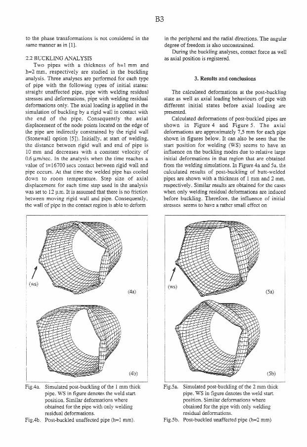
B3

to the phase transformations is not considered in the same manner as in [1].

2.2 BUCKLING ANALYSIS Two pipes with a thickness of h=l mm and

h=2 mm, respectively are studied in the buckling analysis. Three analyses are performed for each type of pipe with the following types of initial states: straight unaffected pipe, pipe with welding residual stresses and deformations, pipe with welding residual deformations only. The axial loading is applied in the simulation of buckling by a rigid wall in contact with the end of the pipe. Consequently the axial displacement of the node points located on the edge of the pipe are indirectly constrained by the rigid wall (Stonewall option [5]). Initially, at start of welding, the distance between rigid wall and end of pipe is 10 mm and decreases with a constant velocity of 0.6 jxm/sec. In the analysis when the time reaches a value of t= 16700 sees contact between rigid wall and pipe occurs. At that time the welded pipe has cooled down to room temperature. Step size of axial displacement for each time step used in the analysis was set to 12 u.m. It is assumed that there is no friction between moving rigid wall and pipe. Consequently, the wall of pipe in the contact region is able to deform

Fig.4a. Simulated post-buckling of the 1 mm thick pipe. WS in figure denotes the weld start position. Similar deformations where obtained for the pipe with only welding residual deformations.

Fig.4b. Post-buckled unaffected pipe (h=l mm).

in the peripheral and the radial directions. The angular degree of freedom is also unconstrained.

During the buckling analyses, contact force as well as axial position is registered.

3. Results and conclusions

The calculated deformations at the post-buckling state as well as axial loading behaviours of pipe with different initial states before axial loading are presented.

Calculated deformations of post-buckled pipes are shown in Figure 4 and Figure 5. The axial deformations are approximately 7,5 mm for each pipe shown in figures below. It can also be seen that the start position for welding (WS) seems to have an influence on the buckling modes due to relative large initial deformations in that region that are obtained from the welding simulations. In Figure 4a and 5a, the calculated results of post-buckling of butt-welded pipes are shown with a thickness of 1 mm and 2 mm, respectively. Similar results are obtained for the cases when only welding residual deformations are induced before buckling. Therefore, the influence of initial stresses seems to have a rather small effect on

Fig.5a. Simulated post-buckling of the 2 mm thick pipe. WS in figure denotes the weld start position. Similar deformations where obtained for the pipe with only welding residual deformations.

Fig.5b. Post-buckled unaffected pipe (h=2 mm)

B4

the buckling modes and the deformations in general. It is also seen from Figure 4 and Figure 5 that the influence of welding on the buckling modes is more pronounced for the pipe with thickness of 1 mm than for the latter.

Calculated axial loading behaviours of pipes with different initial states before buckling are shown in Figure 6. The force is normalized and has a maximum value of 1.0 that corresponds to the yield limit for the material. Both unaffected pipes are collapsed at the maximum point which also agree with the higher theoretical critical loads, evaluated as:

N. • ° M 5 E h 2 (1) a

Equation 1 is only valid for the elastic area of material behaviour.

Comparison between the axial loading behaviours of the pipes with induced imperfections and different wall thickness (denoted welded and weld distorted), indicates that the 1 mm pipe is initially collapsed with bifurcations, i.e. nonaxisymmetric buckling, but the 2 mm pipe is not. The latter reaches the limit load and deforms axisymmetrically until bifurcation-buckling occurs first when the axial deformation is about 1.5 mm.

0.80 i • ' £ 1 1

0.5 0.6 0.7 0.8 0.9 1.0 (mm)

Fig.6. Calculated Load-Displacement path for the considered two pipes.

It is also seen in Figure 6 that the results indicates that the welding residual stresses have a rather small influence on the critical load limit. Therefore the conclusion is that critical load limit for welded pipes with radius-to-thickness ratios of 50 to 100 is mainly due to initial deformations. Thus, welded pipes with less radius-to-thickness ratios than the thin walled pipe studied in [4], deformations due to welding still have a main effect on the load carrying capacity.

5. References

(1) Karlsson, L., Jonsson, M., Lindgren, L.E., Näsström, M. , and Troive, L., Residual Stresses and Deformations in a Welded Thin-Walled Pipe, The American Society of Mechanical Engineerings (ASME), PVP-Vol.173, Residual Stresses and Plastic Deformation (Book no. H00488), pp.7-11, 1989.

(2) Brush, D.O., and Almroth, B.O., Buckling of Bars, Plates, and Shells, McGraw-Hill Book Company, New York, 1975.

(3) Hutchinson, J.W., and Koiter, W.T., Postbuckling theory, Appl. Mech. Rev., Vol.23, pp.1353-1356, 1970.

(4) Häfner. L . , Einfluß einer Rundschweißnaht auf die Stabilität und Traglast des axialbelasteten Kreiszylinders, Doctoral Thesis, Univ. of Stuttgart, FRG, 1982.

(5) NIKE3D: A Nonlinear, Implicit, Three-Dimensional Finite Element Code for Solid nd Structural Mechanics, Hallquist, J.O., University of California, Lawrence Livermore National Laboratory, Rept. UCID-18822,1990.

(6) Karlsson, L., and Lindgren, L.E., Combined Heat and Stress-Strain Calculation, Modeling of Casting, Welding and Advanced Solidification Processes V, The Minerals, Metals & Materials Society, pp.187-201, 1991.

(7) STEPP: Shell Thermo Elasto Plastic Program. No documentation.

(8) Carslaw, H.S., and Jaeger, J.C, Conduction of Heat in Solides, University Press, Oxford, 1959.

(9) Lindgren, L.E., and Karlsson, L., Deformations and Stresses in Welding of Shell Structures, International Journal for Numerical Methods in Engineering, Vol.25, PP.635-655,1988.

Paper C

C l

Numerical and Experimental Study of Residual Deformations due to Double-J Multi-Pass

Butt-Welding of a Pipe-Flange Joint

Lars Troive University College of Falun/ Borlänge

S 781 10 Borlänge

Mikael Jonsson Luleå University of Technology

Sweden S 971 87 Luleå

Sweden

ABSTRACT

A butt-joint between a flange and one end of a pipe is studied. Both the pipe and flange are made of 316 stainless steel. The joint is made up of 11 weld passes, deposited from both sides of the flange. Deformations and stresses during and after welding of the pipe-flange joint are calculated using the Finite element method. The residual deformations are compared with corresponding experimental quantities. In the numerical simulation, heat flow in the circumferential direction is neglected. The problem is therefore treated as rotational symmetric. The supply of weld material during each weld pass is modelled with the socalled "born-die technique". Both base and weld material are assumed to be thermo-elasto plastic. Temperature dependence of the material properties are accounted for, and convective surface heat transfer and heat conduction are considered in the model. In the experiments manual metal arc-welding technique was used. Voltage and current were recorded for each weld-pass in order to have correct heat input in the simulation. The temperature in the pipe was measured at two positions during welding for estimation of the arc efficiency. The residual deformations were obtained by careful measurement of the geometry of the pipe and flange before and after welding. Qualitatively good agreement between calculated and measured deformations was obtained.

INTRODUCTION A common type of pipe joint in many applications is the flange joint (e.g., in process and offshore industry). The

main advantage of this joint compared to a butt-welded joint is the much easier handling during mounting and unmounting of parts in the system. It is also often the best type of joint when the two pipes to be connected are made of different materials.

The flanges of the two pipes are usually bolted together directly through the flange that is fixed to the pipe, or by an extra loose flange that is connected with bolt joints to a fixed or loose flange on the other pipe. In both cases it is essential that the contact surface of the flange that is fixed to the pipe is planar, so leakage out from the pipe is prevented.

2

Figure 1. Geometry of pipe and flange with double-J groove.

C2

When manufacturing a pipe with a flange, usually the flange is machine turned and then attached to the end of the pipe by a weld joint. Due to welding-induced thermal stresses, both the pipe and flange deform, and especially the flange has an undesired shape after welding. This means that further machine work must be carried out on the flange to get the final geometry. How the flange is distorted (twisted) depends on the groove shape and the welding sequence. It is desirable to get as small distortions as possible so machining after welding can be minimized. It would be even better i f the distortions for a specified welding sequence could be predicted. The flange could then be manufactured with a geometry where the distortions are considered. After welding together the pipe and flange, a plane contact surface would then be obtained. In order to make such predictions, numerical models that consider all types of thermomechanical phenomena that occur during welding must be developed.

Thermomechanical modelling of welding using Finite element technique was first reported more then ten years ago, and today reliable predictions of stresses and deformations in butt-welded pipes and plates can be carried out (see for example [1-4]). When it comes to modelling the welding of a flange to a pipe, very little is reported, and especially on welding distortions, no numerical modelling can be found in the litterature.

PRESENT INVESTIGATION The aim of this work is to study the residual deformations that occur after welding a flange to one end of a pipe.

An experimental and a careful numerical study are performed with the objective to "tune" the numerical model until good agreement between experiments and calculations is obtained.

With a reliable numerical model, the next step is to vary the welding procedure until the deformations in the flange are minimized. I f the twist after welding of the flange cannot be small enough, one should at least be able to predict the size and shape of it. Then it would be possible to compensate for the twist during manufacturing of the flange so it after welding would have the desired shape. Such an investigation will be the natural continuation of this work.

The pipe in this work has an inner radius of 84 mm, wall thickness of 8 mm and the length of the pipe is 200 mm. The flange has an outer radius of 134 mm and an inner radius of 92 mm. The thickness of the flange is 22 mm. Both pipe and flange are made of 316 stainless steel. The flange is fixed near to one end of the pipe by the use of a multi­pass welding technique. The geometry is shown in Fig 1. The joint between pipe and flange was made up by 11 weld passes, where the passes were laid in order 1 to 11, see Fig 2.

Comparisons between experiments and calculations concerns the residual deformations after welding in both the pipe and the flange.

EXPERIMENTS EXPERIMENTAL ARRANGEMENTS

The pipe was made of two plates which were previously bent into half circular cross section profiles and then longitudinally welded together. The flange was finish turned to the cross section shown in Fig 1. The groove shape and the amount of filler material used was done according to Swedish codes for this type of welded joint, SS 06 41 01. The flange was fixed to the pipe by use of four tack welds. The tack welds were about 10 mm long and placed symmetrically in the circumferential direction. The tack welding was performed in the bottom of the groove on the negative side. Negative side means that the out going normal on the surface of the flange is directed in the negative z-coordinate direction, see Fig 1.

A l l welding was performed in horizontal position, meaning that the pipe was standing on one or the other of its ends depending on which of the passes that were laid.

The butt-joint between the flange and the pipe was made up by 11 weld passes. The order in which they were deposited is shown in Fig 2. The welding was performed with a manual metal arc welding technique, and the electrodes used were of type "Avesta SKR AC/DC". During welding, current and voltage were registered for each pass. Also welding time/rest time was recorded during the whole process. Since a manual metal arc welding technique was used, slag had to be removed after each stop. The welding parameters for each pass are given in Table 1. The gross heat input for each pass shown in Table 1 is given by the product between current, voltage and accumulated welding time.

TEMPERATURES In order to determine the arc efficiency for each pass, temperatures were measured at two points on the inner

surface of the pipe during welding. The maximum temperature at these two points were compared with corresponding calculated values in the simulation, and the heat input in the simulation was adjusted until good agreement between calculated and measured temperatures was obtained. This procedure gave an arc efficiency of 0.7 for all passes.

C3

The temperatures were measured with Ni-CrNi thermocouples. The thermo-couples were spot welded to the pipe, and time histories of the temperatures were plotted. The maximum temperatures and the temperature at the beginning of each pass for the two positions are given in Table 1.

RESIDUAL DEFORMATIONS Residual deformations were determined on both the pipe and the flange. Residual deformations are the

deformations of the structure due to welding when the pipe and flange have cooled down to room temperature. On the pipe the diameter change was measured in four circumferential positions (every 45 degree), and for each of these positions at every 5 mm from the positive surface of the flange (z=40 mm) to the upper end of the pipe (z=190 mm). The measurements were performed on the outer surface of the pipe. On the flange the diameter change and the relative deflection in z-direction were measured. The diameter change was measured at the same circumferential positions as for the pipe, and for each circumferential position at three points in z-direction: at the middle of the height of the flange, and 7 mm on both sides from the middle (in the coordinate system shown in Fig 1, meaning at z= 14, 21 and 28 mm). The diameter change of both the pipe and the flange were obtained by measuring the diameter before and after welding. The difference between measured diameters gave the desired quantity. The diameter was measured with a micrometer screw. To obtain proper results from such a measurement it was necessary to put the device in the exact same points in the two readings (before and after welding). Therefore the surfaces were smooth grinded, permanent marks were made on the surface and pointed ends on the micrometer screw were used. Similar technique have been used earlier for repeatable measurements of residual deformations, see [1] and [2].

The relative deflection of the flange in z-direction was measured on the negative side (z= 10 mm) of the flange. The final pipe with flange was put on a measuring table and the deflection was measured with a dial indicator at every 45 degree in circumferential direction, as well as for each circumferential position at four different radii, r= 110, 115, 125 and 135 mm. As the absolute coordinates in the z-direction were not determined before welding, only the relative deflection between the outer radii and r= 110 mm could be established.

CALCULATIONS Deformations and stresses during and after welding of the pipe-flange joint are studied numerically using an in-

house FE-code (L.E. Lindgren, Div. of Computer Aided Design, Luleå University of Technology, Sweden). A fully three-dimensional FE-analysis of multi-pass welding is associated with certain problems with respect to

unreasonable computer-times even when today's super-computers are used. Therefore a simplified approach was employed where rotational symmetry is assumed by neglecting the effects of the heat flow in the circumferential direction. The assumption of rotational symmetry means that a cross-section of pipe and flange was studied.

Large deformations were accounted for in the mechanical analysis. Thermodynamic coupling was not considered, i.e. heat generation by plastic straining of the material was neglected, and the mechanical field was coupled to the temperature field only through the temperature-dependent constitutive properties and thermal strain. The mechanical analysis was performed after the thermal analysis in each time increment. To simulate the supply of weld material the "born-die technique" was used. This option has been implemented during this present work and this technique is described in more detail later in this paper. The thermal loadings, representing the energy from the 11 passes of welds, were applied as nodal heat input in each cross section area of weld pass. The thermo mechanical analysis was performed for times t=0 to t=26000 sec using about 1200 time steps.

FINITE ELEMENT MODEL The cross section of the structure, including pipe, flange and weld material is divided into 1476 four-node

elements with bilinear base functions using 1560 nodal points. The Finite element mesh used in thermal and mechanical analyses is shown in Fig 3. Since the model consists of finite elements representing the eleven passes of welds, the "born-die technique" is used to simulate the supply of weld material. The weld elements are unactivated until the time for BIRTH when the front of the simulated heat source is passing the plane for simulation. The shape and area of each cross section of weld pass in the model was estimated from the gross heat input energy due to the proportionality between energy and deposited volume of melted filler material. In the FE-model a simplified approach was employed neglecting the effects of the gap between flange and pipe. A numerical test was performed where essential zero stiffness was assigned to elements very close to the inner radius of the flange simulating the effects of the gap. Negligible effects were obtained.

THERMAL PROPERTIES The temperature-dependent thermal properties (thermal conductivity X and heat capacity c) were taken from [7].

The same thermal material properties were assumed for both base and weld material. The temperature variations of the thermal conductivity X and the heat capacity c are shown in Fig 6. The high value of the heat capacity c (taken

C4

from [6]) between solidus temperature 1495 °C and liquidus temperature 1530 °C corresponds to a latent heat of 260 kJ/kg. For temperatures higher than the solidus temperature the value of thermal conductivity X was given a value of 230 W/m°C (taken from [6]). Also the convective surface heat transfer coefficient between steel and air was taken from [6] with the value of 12 W/m 2.

MECHANICAL MATERIAL PROPERTIES Both weld and base material were assumed to be thermo-elastoplastic with temperature-dependent material

properties. The following parameters were needed in the mechanical analysis, modulus of elasticity E, poisson's ratio v, hardening modulus H', thermal dilatation eT and yield stresses ar. The mechanical material parameters E,

v, and H for base material were obtained from [5], except for the values of poisson's ratio v, above 400 °C, which were assumed to increase up to a level of 0.47. The modulus of elasticity E and poisson's ratio v for weld material were assumed to be the same as for the base material. The temperature dependence of E and v is shown in Fig 4 and 5 respectively. The hardening modulus H for weld material was taken from [9] and it so happened that the parameter agreed with the hardening modulus for the base material (see Fig 5). The thermal dilatation sT for base and weld material was obtained from [7]. The thermal dilatation curve shows that no solide phase transformations occur (see Fig 5). The yield stress parameters at (base material) and cr, (filler material) were obtained from [8] and

[9], respectively. The temperature dependence of ah and af is shown in Fig 4.

THERMAL ANALYSIS

For the thermal analyses two subincrements were used, which means that during one time step for the mechanical analysis, two thermal analyses were performed. The initial temperature was 20 °C. Since the heat energy input in the weld depends on the arc efficiency 77, comparisons between calculated temperatures and measured temperatures were made giving the best agreement. The arc efficiency 77 was estimated to be 0.7 for all weld-passes. In the thermal analysis convective surface heat transfer between steel and air was considered except for the surface of the weld material. Unactivated elements were constrained to be 20 °C in the thermal analyses until time for BIRTH. At this time t=t D , thermal loading was applied as nodal inputs into the current elements. The heat input energy for each weld pass was linearly increased from zero at the time for t=tb, to constant value in the interval [ t D + t i , tb+t2] and then linearly decreased to zero at time t=tD+t3. The time interval t3 for loading is dependent on the heat-source velocity i.e. time for the heat-source to pass the plane for simulation. The data for the gross heat input Q and the times tb, 1 1 , 1 2 and 1 3 for each weld pass are shown in Table 2. In Fig 7 a schematic graph of the heat input function is shown, including the times tb, t ] , t2 and t3.

In the experiment a break occurred during weld pass number four. The rest of weld pass number four and the subsequent passes were applied after cooling to room temperature. In the simulation the total heat input from weld pass number four is applied after the break.

MECHANICAL ANALYSIS Large deformations were accounted for in the mechanical analysis. The filler material was activated at time t=t(-,

(tb is the time for BIRTH for each weld pass). This means that changes in material data as well as the thermal loading were applied at the same time. From a physical point of view, when the weld material is deposited into the groove, the cooling phase takes place immediately and only negative dilatations occur, but in the rest of the structure, the heating and the cooling phase give both positive and negative dilatations. Therefore, no expansions of the weld material were permitted during heating. Furthermore, the thermal strain increment was set at zero for temperatures above 1100 °C. Numerical problems with respect to convergence in plastic strains were avoided with the "so-called" Suppression-method [3]. Using the Suppression-method means that material within and close to the melted zone that has reached temperatures above 1100 °C is deformed only elastically.

MODELING OF SUPPLIED MATERIAL As mentioned before, the "born-die technique" was used, simulating the supply of weld material. This option has

been implemented during this present work, into an in-house FEcode. Using this technique in multi-pass welding simulation is associated with certain problems according to distortions of unactivated elements, as mentioned in [4], due to the fact that nodes in the interface-region between activated and unactivated elements i.e. nodes lying on the edge of the weld groove, are able to move but the rest of the unactivated element-nodes are not. The consequence is that an unactivated element with at least one unconstrained node is liable to large distortions, caused by the very low modulus of elasticity assigned to the element. I f the magnitude of deformation field in the neighbourhood of the simulated weld exceeds the size of the unactivated elements i.e. element size is very small in the weld region, numerical problems occur and the computation will break down i f large deformations are accounted for. Therefore

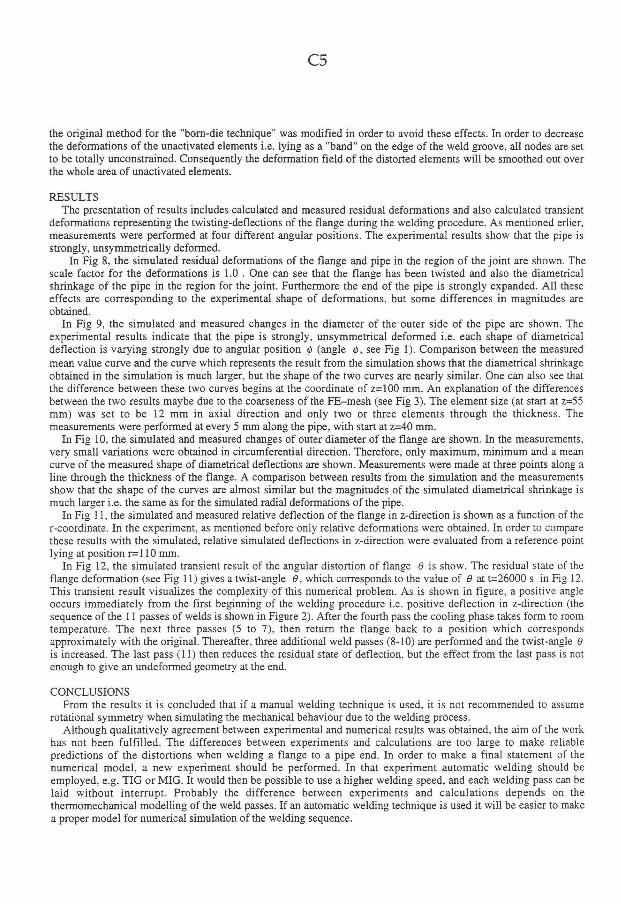
C5

the original method for the "born-die technique" was modified in order to avoid these effects. In order to decrease the deformations of the unactivated elements i.e. lying as a "band" on the edge of the weld groove, all nodes are set to be totally unconstrained. Consequently the deformation field of the distorted elements will be smoothed out over the whole area of unactivated elements.

RESULTS The presentation of results includes calculated and measured residual deformations and also calculated transient

deformations representing the twisting-deflections of the flange during the welding procedure. As mentioned erlier, measurements were performed at four different angular positions. The experimental results show that the pipe is strongly, unsymmetrically deformed.

In Fig 8, the simulated residual deformations of the flange and pipe in the region of the joint are shown. The scale factor for the deformations is 1.0 . One can see that the flange has been twisted and also the diametrical shrinkage of the pipe in the region for the joint. Furthermore the end of the pipe is strongly expanded. A l l these effects are corresponding to the experimental shape of deformations, but some differences in magnitudes are obtained.

In Fig 9, the simulated and measured changes in the diameter of the outer side of the pipe are shown. The experimental results indicate that the pipe is strongly, unsymmetrical deformed i.e. each shape of diametrical deflection is varying strongly due to angular position tp (angle <j>, see Fig 1). Comparison between the measured mean value curve and the curve which represents the result from the simulation shows that the diametrical shrinkage obtained in the simulation is much larger, but the shape of the two curves are nearly similar. One can also see that the difference between these two curves begins at the coordinate of z=100 mm. An explanation of the differences between the two results maybe due to the coarseness of the FE-mesh (see Fig 3). The element size (at start at z=55 mm) was set to be 12 mm in axial direction and only two or three elements through the thickness. The measurements were performed at every 5 mm along the pipe, with start at z=40 mm.

In Fig 10, the simulated and measured changes of outer diameter of the flange are shown. In the measurements, very small variations were obtained in circumferential direction. Therefore, only maximum, minimum and a mean curve of the measured shape of diametrical deflections are shown. Measurements were made at three points along a line through the thickness of the flange. A comparison between results from the simulation and the measurements show that the shape of the curves are almost similar but the magnitudes of the simulated diametrical shrinkage is much larger i.e. the same as for the simulated radial deformations of the pipe.

In Fig 11, the simulated and measured relative deflection of the flange in z-direction is shown as a function of the r-coordinate. In the experiment, as mentioned before only relative deformations were obtained. In order to compare these results with the simulated, relative simulated deflections in z-direction were evaluated from a reference point lying at position r=l 10 mm.

In Fig 12, the simulated transient result of the angular distortion of flange 8 is show. The residual state of the flange deformation (see Fig 11) gives a twist-angle 0, which corresponds to the value of 8 at t=26000 s in Fig 12. This transient result visualizes the complexity of this numerical problem. As is shown in figure, a positive angle occurs immediately from the first beginning of the welding procedure i.e. positive deflection in z-direction (the sequence of the 11 passes of welds is shown in Figure 2). After the fourth pass the cooling phase takes form to room temperature. The next three passes (5 to 7), then return the flange back to a position which corresponds approximately with the original. Thereafter, three additional weld passes (8-10) are performed and the twist-angle 8 is increased. The last pass (11) then reduces the residual state of deflection, but the effect from the last pass is not enough to give an undeformed geometry at the end.

CONCLUSIONS From the results it is concluded that i f a manual welding technique is used, it is not recommended to assume

rotational symmetry when simulating the mechanical behaviour due to the welding process. Although qualitatively agreement between experimental and numerical results was obtained, the aim of the work

has not been fulfil led. The differences between experiments and calculations are too large to make reliable predictions of the distortions when welding a flange to a pipe end. In order to make a final statement of the numerical model, a new experiment should be performed. In that experiment automatic welding should be employed, e.g. TIG or MIG. It would then be possible to use a higher welding speed, and each welding pass can be laid without interrupt. Probably the difference between experiments and calculations depends on the thermomechanical modelling of the weld passes. I f an automatic welding technique is used it will be easier to make a proper model for numerical simulation of the welding sequence.

C6

REFERENCES 1. L. Karlsson, M. Jonsson, L E . Lindgren, M . Näsström, and L. Troive, "Residual Stresses and Deformations

in a Welded Thin-Walled Pipe", in Weld residual stresses and plastic deformation, Eds. E. Rybicki, M . Shiratori, G. E. O. Widera, and T. Miyoshi, The American Society of Mechanical Engineers, PVP- Vol 173, Book No H00488- 1989,pp 7-11.

2. M . Jonsson, B.L. Josefson, and M. Näsström, "Experimentally Determined Deformations and Stresses in Narrow-Gap and Single-U Multi-Pass Butt-Welded Pipes", ASME, inJournal of Offshore Mechanics and Arctic Engineering, May 1993, Vol 115. pp 116-122.

3. B.L. Josefson, and R.I. Karlsson, "Finite Element Analysis of In-Plane Deformations and Stresses in Restrained Butt Welded Plates", Presented at "International Conference on The Effectts of Fabrication Related Stress on Product Manufacture and Preformance", The Welding Institute, Abingdon, UK, Sept. 1985.

4. B.L.Josefson, and C.T. Karlsson, "FE-Calculated Stress in a Multi-Pass Butt Welded Pipe- A simplified approach", in Int. J. Pressure. Vessels Piping, No 38 (1989),pp. 227-243.

5. E. F. Rybicki, D. W. Schmueser, R. B. Stonesifer, J. J. Groom, and H. B. Mishler,"A Finite Element Model of Residual Stresses in Girth-Butt Welded Pipes", Presentated at the 1977 ASME W A M , Numerical Modeling of Manufacturing Processes, PVP-PB-025, Dec. 1977, pp. 1-18.

6. M . Jonsson, L. Karlsson, and L.E. Lindgren, "Deformations and Stresses in Butt-Welding of Large Plates", in Numerical Methods in Heat Transfer-Volume III, ed. by R.W. Lewis, and K. Morgan, Wiley, London, 1985.

7. J Friedrich Stelzer, in Physical Property Algorithms/ Stoffwertalgorithmen, Thiemig-Taschen biicher, band 93, (K. Thieming ag München, 1984, ISBN 3-521-06144-2)

8. Sandvik Steel (S-l, 842-ENG,May 1991) Sandvik 5R60 AISI type 316

9. Avesta Welding AB, SWEDEN (Mr. Björn Holmberg)

TABLES AND FIGURES

Current Voltage Accumrr Aooumu- Heat Heat Tinit. Ttnit. Tmax. Tmax. luted lated input inputs z-lSmm r=25 mm Z=15mm z=25 mm

welding rest length (A) (V) time Is) t ime i» (MJ) (MJ/m) CO CO CO CO

i 56 25 233 422 0,326 0.54 20 20 132 232 2 78 27 214 162 0.451 0.75 80 80 225 275 3 KK) 27 185 97 0.5 0.83 157 170 [275] [300]

4a 58-64 22-24 178 246 0.246 / 182 195 355 295

4b 79 28 135 517 0,299 0,9 20 20

5 82 30 172 358 0.423 0,705 35 40 330 220

6 82 30 194 322 0.477 0,795 82 94 335 245

7 102 28 186 368 0,531 0.885 150 157 405 298 S 130 27 161 188 0,565 0.942 238 235 341 496

9 148 79 0.519 0,865 260 291 [320] [375]

10 172 179 0,604 1,007 318 342 360 501 11 iii 28-30 167 148 0,654 1,09 320 344 530 420

Line energy

Q (MJ/m)

Velocity

(mm/s)

MTH-iimc I

tb

(s)

I imes lor trie Heat Input Function Line energy

Q (MJ/m)

Velocity

(mm/s)

MTH-iimc I

tb

(s)

tl

<*)

t l

<s> 13 (s)

1 3.78E-OI 2,6 0 1,46 4,36 5,81

2 5.25E-01 2.8 655 1.34 3.99 5.31 3 5.81E-01 3.3 1031 1,16 3,46 4,61 4 6.30E-01 1.9 1313 2,01 6,01 8.01

5 4.94E-01 3,5 12389 1,09 3.24 4,31

6 5.56E-01 3,1 12919 1.24 3,69 4,91

7 6.19E-01 3.2 13435 1.19 3.54 4.71 8 6.59E-01 3,7 13989 1,01 3,01 4.01

9 6.30E-01 4,1 14338 0,94 2,79 3,71

10 4.23E-01 3,5 14565 1,09 3,24 4.31 11 4.58E-01 i,6 14916 1,06 5.16 4,21

Table 1. Registered and recorded data during experiment.

Table 2. Heat input data for the thermal analysis.

C7

Figure 4. Modulus of elasticity E( for base and filler Figure 5. Poisson's ratio v, hardening modulus H' material) and yield stresses tr„(base material) and a nd thermal dilatation eT, as functions of cr, (filler material), as functions of temperature. temperature. Same parameters are used for both base

and filler material.

and

0 500 1000 1500 2000 Temperature (°C)

C8

100 150 z-cxwrdinate (mm)

Figure 9. Measured and calculated diametrical deflection of pipe. The angle tp represents the angular positions in circumferential direction for which measurements were performed.

120 125 r-coordinate (mm)

Figure 11. Measured and calculated relative deflections of flange in z-direction.

Figure 8. Calculated residual deformations of pipe and flange. Scale factor for displacements in figure is 1.0 .

15 20 25 30 z<ooidinate (mm)

Figure 10. Measured and calculated diametrical deflections of flange, as functions of z-coordinate.

T m e (s)

Figure 12. Calculated transient result of angular distortions 6 of flange during welding procedure. Each peak represents the heating phase when weld pass is applied.

Paper D

D l

EXPERIMENTAL AND NUMERICAL STUDY OF MULTI-PASS WELDING PROCESS OF

PIPE-FLANGE JOINTS

* Department of Mechanical Engineering, University College of Dalarna, S 781 10, Borlänge, SWEDEN ** Division of Computer Aided Design, Luleå University of Technology, S 971 87 Luleå, SWEDEN

Residual deformations of pipe-flange joints due to thermal strains caused by the multi-pass welding procedure in a manufacturing process are investigated both experimentally and numerically. When a pipe-flange joint is manufactured a flange is attached to one end of a pipe by multi-pass welding. Consequently large residual stresses are induced and residual deformations as well. To avoid any risk of leakage between two mounted pipes geometrical distortions (twisting) of the flange must be prevented. How the flange is distorted depends both on the groove shape and the weld sequence used. However, to be spared from machine work after the welding process the distortions have to be minimized. During present work and in a recent project performed, reported in [1 ] , a numerical model has been developed and implemented in an in-house FE-code in order to predict the residual deformations of flange and pipe. In addition to the numerical part of the investigation work has been devoted to experimental verification of results. A casting-technique has been developed in order to measure the twisting of the flange after each weld pass. Also measurements of the residual radial deflection of the pipe have been performed by use of a coordinate-measuring machine. In order to estimate the arc efficiency temperatures were measured at three points during the experiment. In the experiment four pipe-flange joints were considered, two made of stainless steel 2352 and the other two made of Swedish steel 2142. For each type of material two multi-pass sequences were used. Numerical simulations of the multi-pass welding of pipe-flange joints are performed for the stainless steel type of material and compared with experimental results

L. Troive * , M . Näsström ** and M . Jonsson**

A B S T R A C T

Figure 1. Geometry of pipe and flange considered

D2

I N T R O D U C T I O N

Components of piping systems in the process and offshore industries are often joined together with a flange joint. This flange joint has proved itself to be the best joint i f pipes of different material are to be connected. Another advantage of this type of joint is the easy handling of parts when mounting and dismantling piping systems. I f pipes within a piping system are to be connected with flange joints i t is important that the contact surface of the flange which is fixed to the pipe is plane in order to prevent leakage.

When a pipe with a flange is manufactured, usually the flange is machine turned and then attached to the pipe with a weld joint. This weld introduces residual stresses in the component which causes the pipe and flange to deform. This deformation is often of such magnitude that further machine work must be carried out on the flange after welding to receive the desired geometry. As distortion (twisting) of the flange is not desired, it is important to arrange the welding of the flange to the pipe in such a way that machining after welding is minimized, or even better avoided. Another way of avoiding twisting of the flange is i f the distortion can be numerically predicted, the flange geometry can be manufactured in such a way that a plane contact surface on the flange is obtained after welding. The distortion of the flange depends on the groove shape, number of weld passes and the welding sequence. Prediction of the distortion of the flange can be numerically made by use of numerical methods, such as the finite element method, i f they take into consideration the thermomechanical phenomena that occur during welding [1].

Present investigation

The main purpose of this investigation is to experimentally detect and numerically simulate the deformations that occur during and after welding of a flange to one end of a pipe. As reported in [1], deformations can be predicted satisfactorily using the finite element method. In this investigation, a similar finite element model as in [1] has been used to simulate the deformations. The code has been improved to even better consider the mechanical phenomena involved in this welding procedure. A careful experimental study is performed where the objective is to detect the flange distortion during welding and both the flange and pipe distortion after welding.

In this work, four cases (A-D) have been studied. In each case a flange has been welded to one end of a pipe by use of multi-pass welding technique. The material in the flange and the pipe is, in case A and B, stainless steel and in case C and D, ordinary steel. The difference between case A and B and between C and D is in what order the weld passes are deposited. See Figure 2.

In all four cases (A-D) the geometry of the pipes and the flanges was the same. The pipepipe has an outer diameter of 90 mm, wall thickness of 9.5 mm and a length of 300 mm. The flange has an outer diameter of 150 mm, an inner diameter of 90.5 mm and a thickness of 15 mm. The joint between the pipe and the flange is made by 10 weld passes. This investigation shows that numerical simulations (FEM) can predict the deformations in this type of components fairly well.

D3

E X P E R I M E N T S

Experimental arrangements

The two stainless steel pipes used in the experiments (A and B) were finish-turned on the outside to ensure that the wall thickness was equal to the wall thickness of the ordinary steel pipes (C and D). The flanges were tack-welded to the pipe with four tack-welds, each 10 mm long, and equally spaced around the circumference. Theese tack-welds were placed at the bottom of the groove situated on the negative side of the flange. Negative side means that the outgoing normal of the surface of the flange is directed in the negative z-coordinate direction, see Figure 1. In all four experiments, the pipe and flange to be joined rotated with constant angular velocity and the welding torch was held fixed.

The joint between the flange and the pipe was made by 10 weld passes. The order of the weld passes for case A and C is shown in Figure 2a and the order of the weld passes for case B and D is shown in Figure 2b. Automatic gas-tungsten welding equipment , ESAB PROTIG 315 INVERTER in combination with a tilting-rotational-fixture system ESAB A25, was used in all experiments. The equipment was computer controlled which means that current, voltage, welding speed, gas f low and feeding speed could be programmed for the whole welding process. Welding parameters in all four experiments are given in Table 1. The gross heat input with estimated arc efficiency included is given in Table 2.

Temperature measurements

In order to determine the arc efficiency for each pass, temperatures were measured at three points: z=5mm, z=17.5mm and z=25mm, on the inner surface of the pipes during welding.

A l l three points were located at 6=Tt where 9=0 is at weld start see Figure 1. The maximum temperature at these points for the two experiments (case A and B) was compared with coresponding calculated temperatures in the simulation. The heat input in the simulations was adjusted until good agreement between calculated and measured temperatures was obtained. This procedure gave an arc efficiency of 0.65 for all passes.

The temperatures were measured with Ni-CrNi thermocouples, which were spot welded to the inner surface of the pipe. The temperature at the beginning of each weld pass and the maximum temperature of each weld pass for the three positions are given in Table 3.

Twisting of flange during process

The twisting angle after each weld pass was obtained by use of a casting technique. In this technique, a dental foam PRO V I L [2], is used as cast compound. PRO V I L has proved itself to have advantageous material characteristics at high temperature. Due to these material characteristics, very small shrinkage is obtained when this material is cured and cooled from high temperature to room temperature. This means that casting using this material is possible at high temperatures.

Measurements of the twisting angle of the flange were performed before the multipass welding started and after each weld pass and finally when the welded pipe flange joint had cooled to room temperature. In these measurements, a flat smooth grinded circumferential plate was used as reference plane. This plate has three sharpened spikes located symetrically on a circle with a diameter as the mean diameter of the pipe. At the time of measurement three, well sized, pieces of the dental foam were symetrically placed on the plate, which thereafter was placed with the

D4

spikes positioned on the end of the pipe i.e. z=0 mm. In this measuring procedure, the dental foam is pressed between the flange and the reference plate, see Figure 3. The spikes as well as the dental foam were placed in the same position in all measurements performed. Assuming rotational symmetry, the twisting angle of the flange can be obtained by evaluating the mean profile of these three casted pieces.

Diametrical residual shrinkage

The diametrical residual shrinkage of the pipes investigated was obtained by measuring the geometry before and after welding, using a coordinate measurement machine (CMM). The total number of points measured on each pipe was around 2000. The diametrical shrinkage is given by subtracting the diameter of the pipe before welding from the diameter after welding.

Figure 2a. Figure 2b. Weld sequence used in experiment A and C. Weld sequence used in experiment B and D.

Reference plane

Cast compound

Figure 3. Casting technique used to detect the twisting angle <j) of the flange.

D5

Pass No/ EXP A 1, 6 2-4, 7-9 5, 10

Pass No/ EXP B 1 - 2 3 - 8 9 - 10

Pulse current [A] 1 7 7 188 168

Pause current [Al 9 0 90 80

AVC Pulse [V] 12,3 12,4 12,4

AVC Pause [VI 9 ,3 9.4 9 , 4

Pulse time [sec] 0,2 0,2 0 ,2

Pause time [sec] 0 ,3 0.3 0,3

Wire feed [mm/ sec] 2 0 3 2 21

Weld speed [mm/secl 1.2 1.2 1.3

Pass No/ EXP C 1, 6 2-4, 7-9 5, 10

Pass No/ EXP D 1 - 2 3 - 8 9 - 10 Pulse current [A] 191 197 197

Pause current fAI 90 9 0 8 0 AVC Pulse [V] 12,3 12,9 13 ,0

AVC Pause W] 9 .3 9 .9 10.0 Pulse time [sec] 0,2 0 ,2 0 ,2

Pause time [sec] 0.3 0,3 0 .3 Wire feed [mm/ sec] 2 0 3 2 2 1

Weld soeed [mm/sec] 1.2 1.2 1.3

Table 1. Registered data during experiment A, B, C, and D

F I N I T E E L E M E N T S I M U L A T I O N

Multi-pass welding of a flange to one end of a pipe is studied numerically by using an in-house FE-code [3] .Two analyses are performed simulating experiment A and B. The two pipe joints simulated are made of stainless steel (Swedish code SS 142352) and the geometry is the same for the pipe joints considered as well. The differences in the two models, simulating experiment A and B, are in which order the weld passes are supplied. The two sequences of ten passes of welds considered are shown in Figure 2.

The aim of this numerical study is to simulate the deformation of the pipe and the flange during and after the welding procedure until they have cooled to room temperature, and to investigate the influence of the welding sequence used. It is clear that in the case of multi-pass welding each pass gives a contribution to the residual deformations and so unfortunately do any deviations when modelling. Therefore, to reach a relatively good agreement between numerical analysis and experiment, each pass of weld has to be taken into account carefully and any assumptions or simplifications have to be well-balanced in a physical sense.

Even i f today's super computers are used a fully three-dimensional FE-analysis of multi-pass welding is associated with unreasonable computer times. Therefore, a simplified approach is employed by treating the problem as rotationally symmetric. In this case the assumption of rotational symmetry means that only a cross-section of the pipe, flange and weld material has to be studied numerically and consequently the number of unknowns is reduced essentially. The assumption of rotational symmetry for the type of problem considered, leads to the heat-arc velocity in the model becoming interminably high. Consequently, i f treating the problem as rotationally symmetric, the total amount of weld material in each weld-pass is supplied simultaneously around the pipe. The cross-section of the structure including pipe, flange and filler material is divided into 1150 four-node elements with bilinear base function using 1263 nodal points. In addition to the latter elements eight contact-elements are also used in model to simulate the in reality two free bodies i.e. the flange and pipe, before jointed. Finite-element mesh used in thermal and mechanical analyses is shown in Figure 4.

In the mechanical analysis, large deformations are accounted for. Thermodynamic coupling is not considered, i.e. heat generation due to deformation of the material is neglected, the mechanical field is coupled to the temperature field only through the temperature dependent constitutive properties and thermal strain. In each time step during the thermomechanical analysis, the temperature field is first calculated and immediately after that the mechanical analysis is performed. In the FE-model the supply of weld material is simulated by the so-called "born and die technique", This method has been investigated before and used in the simulation of multi-pass welding, reported in [1]. In addition to [1], conditions for contact between pipe and flange is included into the FE-model. The thermal loading, representing the

D6

energy from the 10 passes of welds, are applied as nodal heat inputs. The nodal heat input was constant distributed over the cross-section area for each weld-pass.

200 r-coordinate (mm)

Figure 4. Finite element mesh used in the thermal and mechanical analyses.

Welding analysis

The temperature dependent thermal properties (thermal conductivity X and heat capacity c) used in the thermal analysis are shown in Figure 5. These parameters are taken from [4], The same thermal material properties are assumed for both base and fi l ler material. As seen in Figure 5, a high value is assigned to the heat capacity between the solidus temperature 1495°C and liquidus temperature 1530°C which corresponds to a latent heat of 260 kJ/kg.

The thermal conductivity \ for temperatures above the solidus temperature is given a value of 230 W/m °C. Convective surface heat transfer coefficient between steel and air is assumed to be 12 W / m 2 (taken from [5]).

D7

The following mechanical material properties (all taken from [1] and [6]), thermal dilatation

et, modulus of elasticity E, poisson's ratio v, hardening modulus H' and yield stress ay, are used in the mechanical analysis. Besides the latter, all parameters are assumed to be the same for both base material and weld material. As mentioned above, the mechanical material properties were taken from [1 ] where both flange and pipe were made of stainless steel, type 316. As the chemical composition of S316 and 2352 is similar, the mechanical material properties used in [i] were also used in the current simulation. In Figure 6, the temperature

dependence of Young modulus E, yield stresses a b (base material) and o~f (filler material) are shown.

The remaining mechanical material properties used, which are hardening modulus H',

poisson's ratio v and thermal dilatation et, are shown in Figure 7.

D8

Two subincrements were used in the thermal analyses, i.e during one time step for mechanical analysis, two thermal steps were performed. The initial temperature before start of welding

was 26 C. Since the heat energy input in weld depends on the arc efficiency, Tl, comparisons between calculated temperatures and measured temperatures were performed giving the best agreement. The arc efficiency, T), was estimated to be 0.65 for all weld passes.

Convective surface heat transfer was considered between steel and air except for the surfaces of weld. The supply of weld material for each weld pass was simulated by activating elements in that particular area. At the time of birth tb,when elements are activated, thermal loading is applied as nodal heat inputs. The heat input energy for each weld-pass was applied by a step function, simulating the moving heat source through the cross-section for simulation. The step function used was linearly increased from zero at the time for birth t b , to a constant value after 2 seconds and was then constant during a time interval depending on current heat source velocity. After that time interval of constant heat input, the function linearly decreased to zero during 2 seconds, giving a total time of heat input. The total line energy input Q, the time when heat input is applied (BIRTH-time, t b ) as well as the total time of heat inputs (Heat-input time), for each weld pass are shown in Table 2.

A Heat input data B Heat input data

Pass Effective Velocity BIRTH-time Heat input Pass Effective Velocity BIRTH-time Heat input No heat input: Q V No heat input: Q V

f MJ/m) [mm/ seel [sec] [seel [MJ/ml [mm/ seel [seel [seel 1 1.12 1,2 0 8,6 1 1,12 1 ,2 0 8,6 2 1,18 1,2 653 8,7 2 1,12 1,2 1 005 8,6 3 1,18 1 ,2 1252 8,7 3 1,18 1,2 1 707 8,7 4 1,18 1 ,2 2010 8,7 4 1,18 1 ,2 261 8 8,7 5 0,98 1,3 2797 8,0 5 1,18 1,2 3363 8,7

6 1,12 1 ,2 3755 8,6 6 1,18 1,2 4198 8,7 7 1,18 1 ,2 4584 8,7 7 1,18 1 .2 501 0 8,7 8 1.18 1 ,2 5221 8,7 8 1.18 1,2 5778 8,7 9 1,18 1 .2 5842 8,7 9 0.98 1,3 6521 8,0

1 0 0,98 1 .3 6659 8,0 1 0 0,98 1,3 7270 8,0

Table 2. Heat input data used in the thermal simulation of experiment A and B.

D9

Modelling of multi-pass welding

In the finite element model simulating the multi-pass welding procedure the "born-die technique" was used. This technique has been investigated, modified and implemented into an in-house fe-code [ 3 ] , reported in [1] . Using this technique for simulation of multi-pass welding, finite elements which represent one weld pass wi l l be activated first when current weld pass is supplied. I f the common "born-die technique" is used, the degrees of freedom for all unique born-die nodes, i.e. nodes which are not shared with an ordinary element, are fully constrained until time of birth. Fully constrained means that current nodes are neither able to move nor change in temperature. A very low stiffness is also assigned to not activated elements. I t was found in [1] and also mentioned in [ 7 ] , that using the common "born-die technique" in simulations of multi-pass welding the computation is associated with several problems due to the distortions of unactivated elements and thereby numerical problems i f large deformations are accounted for. In Figure 8, elements representing base material "c" and unactivated elements "a" and "b" are shown. Using the common "born-die technique", unactivated elements "a", lying as a band along the weld grove, are very sensitive to the deformations of the structure "c", due to the fact that these elements are very soft and also connected with the fully constrained unactivated-elements "b".

Unactivated elements (filler material)

i : Fully constrained nodes

Base material -X 3>

Figure 8. Schematic view of elements distorted, located in the region closed to the weld groove i f the common "born and die technique" is used.

In this case this element (denoted by "a" in figure 8 above) should be extremly distorted when the flange is twisted, due to the fact that the magnitudes of deformations exceeds the size of the very small elements "a". Consequently, when large deformations are accounted for, the computation wi l l break down immediately. Therefore, the "born-die technique" was modified during recent work [1], by changing the conditions for all unique born-die nodes to be totally free, even i f not activated. Consequently, the deformation field of the distorted unactivated elements, i f using this modified method of "born-die technique", wi l l be smoothed out over the area of unactivated elements and thereby high magnitudes of element distortions wil l be avoided.

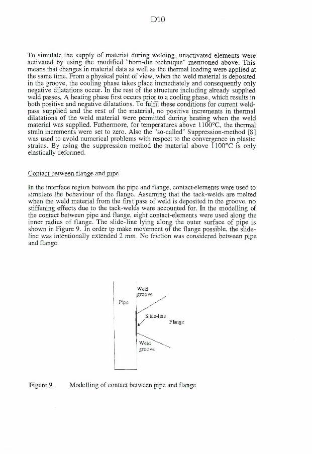
DIO

To simulate the supply of material during welding, unactivated elements were activated by using the modified "born-die technique" mentioned above. This means that changes in material data as well as the thermal loading were applied at the same time. From a physical point of view, when the weld material is deposited in the groove, the cooling phase takes place immediately and consequently only negative dilatations occur. In the rest of the structure including already supplied weld passes, A heating phase first occurs prior to a cooling phase, which results in both positive and negative dilatations. To f u l f i l these conditions for current weld­pass supplied and the rest of the material, no positive increments in thermal dilatations of the weld material were permitted during heating when the weld material was supplied. Futhermore, for temperatures above 1100°C, the thermal strain increments were set to zero. Also the "so-called" Suppression-method [ 8 ] was used to avoid numerical problems with respect to the convergence in plastic strains. By using the suppression method the material above 1100°C is only elastically deformed.

Contact between flange and pipe

In the interface region between the pipe and flange, contact-elements were used to simulate the behaviour of the flange. Assuming that the tack-welds are melted when the weld material f rom the first pass of weld is deposited in the groove, no stiffening effects due to the tack-welds were accounted for. In the modelling of the contact between pipe and flange, eight contact-elements were used along the inner radius of flange. The slide-line lying along the outer surface of pipe is shown in Figure 9. In order tp make movement of the flange possible, the slide-line was intentionally extended 2 mm. No friction was considered between pipe and flange.

Weld groove

Pipe

Slide-line Flange

Weld groove

Figure 9. Modelling of contact between pipe and flange

D i l

R E S U L T S

Temperatures were measured at three points, z=25mm ( T l ) , z=17.5mm (T2) and z=5mm (T3), on the inner surface of the pipes from the start of the welding process until the pipe had cooled to room temperature. Maximum temperatures obtained during welding of each weld pass and minimum temperatures obtained at the beginning of each weld pass are shown in Table 3 and Table 4, for all four cases (A-D). Also times when each weld pass was started and finished are presented in Table 3. Inaccurate temperature data is shown in brackets.

EXP Pass Weld Weld T1 init T2 init T3 init T1 max T2 max T3 max No start stop Z=25 Z=17,5 Z=5 Z=25 Z=17,5 Z=5

[sec] [sec) [mm] [mm] [mm] [mm] [mm] [mm] 1 0 255 29 2 9 29 303 370 396 2 653 910 [1501 [1421 [ 1 4 8 ] 404 473 541 3 1 252 1 508 212 2 0 9 21 1 405 449 490

E 4 2010 2266 233 229 231 436 495 577 X 5 2797 3052 238 234 234 378 416 455 P 6 3756 4008 21 1 2 0 8 2 0 8 494 483 426

7 4584 4840 226 2 2 2 226 512 484 420 A 8 5221 5477 259 260 2 5 7 467 457 426

9 5842 6099 278 2 7 5 2 7 7 507 476 432 1 0 6659 6914 258 256 257 422 414 391 1 0 251 27 2 7 27 297 344 375 2 900 1 152 121 1 1 8 116 384 438 512 3 1 413 1665 208 205 2 0 2 400 438 477

E 4 2121 2373 221 2 1 7 2 1 5 426 473 558 X 5 2646 2902 258 253 250 412 444 476 P 6 6790 7041 64 63 5 9 354 352 301

7 7478 7730 155 153 1 50 470 438 376 C 8 7896 8152 237 234 2 3 2 443 440 414

9 8490 8748 250 2 4 7 2 4 3 502 4 7 3 424 1 0 8902 9157 292 288 284 463 460 437

Table 3. Recorded temperatures during experiments A to C.

EXP Pass Weld Weld T1 init T2 init T3 init T1 max T2 max T3 max start stop Z=25 Z=17,5 Z=5 Z=25 Z=17,5 Z=5

No Isecl fsec] fmml [mml fmml fmml Imml Tmrnl 1 0 252 3 1 3 1 31 319 372 [4111 2 1 005 1257 127 127 121 452 432 379 3 1 707 1963 198 1 97 1 84 458 507 579

E 4 2618 2874 207 207 1 96 521 4 7 8 431 X 5 3363 3615 237 232 2 2 3 438 466 51 0 P 6 4198 4455 238 236 225 466 442 421

7 5010 5307 249 246 236 457 495 585 B 8 5778 6033 253 253 241 51 0 4 5 9 423

9 6521 6775 262 261 250 416 434 473 1 0 7270 7525 258 2 5 7 247 428 4 0 8 395 1 0 252 33 3 3 33 327 360 391 2 1752 2004 81 82 81 353 348 320 3 2507 2766 159 160 1 88 452 486 563

E 4 3331 3589 183 184 1 82 464 440 405 X 5 4248 4505 185 190 1 87 417 434 459 P 6 5147 5404 1 90 192 1 92 4 0 5 396 383

7 6081 6339 1 93 194 1 92 4 3 9 460 544 D 8 7339 7596 159 160 159 414 388 359

9 8165 8421 191 1 96 1 92 383 392 421 1 0 8957 921 3 189 196 195 387 380 371

Table 4. Recorded temperatures during experiments B to D.

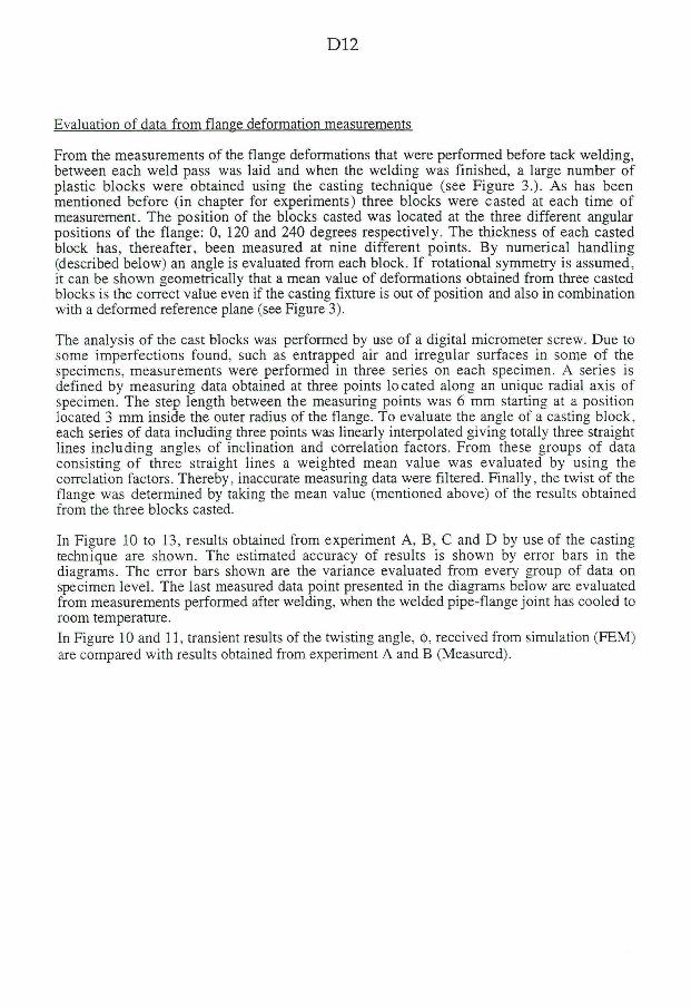
D12

Evaluation of data from flange deformation measurements

From the measurements of the flange deformations that were performed before tack welding, between each weld pass was laid and when the welding was finished, a large number of plastic blocks were obtained using the casting technique (see Figure 3.)- As has been mentioned before (in chapter for experiments) three blocks were casted at each time of measurement. The position of the blocks casted was located at the three different angular positions of the flange: 0, 120 and 240 degrees respectively. The thickness of each casted block has, thereafter, been measured at nine different points. By numerical handling (described below) an angle is evaluated from each block. I f rotational symmetry is assumed, it can be shown geometrically that a mean value of deformations obtained from three casted blocks is the correct value even i f the casting fixture is out of position and also in combination with a deformed reference plane (see Figure 3).

The analysis of the cast blocks was performed by use of a digital micrometer screw. Due to some imperfections found, such as entrapped air and irregular surfaces in some of the specimens, measurements were performed in three series on each specimen. A series is defined by measuring data obtained at three points lo cated along an unique radial axis of specimen. The step length between the measuring points was 6 mm starting at a position located 3 mm inside the outer radius of the flange. To evaluate the angle of a casting block, each series of data including three points was linearly interpolated giving totally three straight lines including angles of inclination and correlation factors. From these groups of data consisting of three straight lines a weighted mean value was evaluated by using the correlation factors. Thereby, inaccurate measuring data were filtered. Finally, the twist of the flange was determined by taking the mean value (mentioned above) of the results obtained from the three blocks casted.

In Figure 10 to 13, results obtained from experiment A, B, C and D by use of the casting technique are shown. The estimated accuracy of results is shown by error bars in the diagrams. The error bars shown are the variance evaluated from every group of data on specimen level. The last measured data point presented in the diagrams below are evaluated from measurements performed after welding, when the welded pipe-flange joint has cooled to room temperature.

In Figure 10 and 11, transient results of the twisting angle, <t), received from simulation (FEM) are compared with results obtained from experiment A and B (Measured).

D13

6

• Mee

FBvl

tsured

l • Mee

FBvl

tsured

i rt

*

i i—

•—i

i i—

•—i

r2

i T • X

O 2000 4000 6000 8000 10000 12000

Time [sec]

Transient result of twisting angle, <j), received from simulations of experiment A, compared with experimental results. The last measurin data point was obtained after cooling down to room temperatur.

ft

0 2000 4000 6000 8000 10000 12000

Time [sec]

Transient result of twisting angle, <j), received from simulations of experiment B compared with experimental results. The last measurin data point was obtained after cooling down to room temperature.

D U

i

<

-1

A" • -

- f -T i

Measured

I I 0 4000 8000 12000 16000

Time [sec]

Figure 12. Measured twisting angle, <j>, obtained after tack welding, after the following passes: 1, 3, 5, 6, 8, 10 and after when cooling to room temperature during experiment C.

r

;.A 1

i •~m~ Measured

r

;.A 1 Jl-. r * i - .

- • - i

0 4000 8000 12000 16000

Time [sec]

Figure 13. Measured twisting angle, <h, obtained before and after each welding pass during experiment D . The last measuring data point was obtained after cooling down to room temperature.

In Figure 14 and 15, the residual deformations of the flange and pipe in the region of the joint obtained from simulation of experiment A and B, respectively, are shown. The scale factor for the deformations in both Figures is 1.0. The residual state of the flange twisting angle obtained f rom case A and B, can be seen. It can also seen that the pipes are strongly shrunk radially in the immediate vicinity of the joint but the end of the pipes is not.

D15

Figure 14. Residual deformations obtained f rom simulation of experiment A. Scale factor for displacement in figure is 1.0 .

Figure 15. Residual deformations obtained from simulation of experiment B. Scale factor for displacement in figure is 1.0 .

The measured and numerically simulated residual radial shrinkage of the stainless steel pipe is shown in Figures 16 and 17. In Figure 18 and 19 the measured residual radial shrinkage of the ordinary steel pipes is shown. It can be seen in Figures 16 and 17 that the maximum magnitude of the measured and simulated shrinkage is almost the same. One can also see that the position on the pipes where the numerically simulated shrinkage starts deviates from the position of the measured ones.

2-coordinate [mm] (Exp A)

0 50 100 150 200 250 300

c

-20

.

N V

SÅ 1 ' Measured

FEM

/

/

j

Figure 16. Measured and simulated residual radial shrinkage of the outer surface of the pipe obtained from case A.

D16

Z-coordinate [mm] (Exp B) 0 50 100 150 200 250 300

-20

I i

/

i M

FE

sasured

M

f f *

Figure 17. Measured and simulated residual radial shrinkage of the outer surface of the pipe obtained from case B.

E 5

Z-coordinate [mm] 100 150

(Exp C) 200

I Measured [

.20 J> 1 1 1 1 1 1

Figure 18. Measured residual radial shrinkage of the outer surface of the pipe obtained from case C.

Z-coordinate [mm] (Exp D)

100 150 200

I Measured!

-20

Figure 19. Measured residual radial shrinkage of the outer surface of the pipe obtained from case D.

D17

DISCUSSION AND CONCLUSIONS

A careful experimental investigation of deformations and residual distortions in pipe and flange arising from the welding procedure of the joint has been presented. Both pipes and flanges made of ordinary and stainless steel are investigated. The welding procedure of the pipe-flange joint in stainless steel has been numerically simulated and compared with the experimental results. Overall, the agreement between numerical and experimental results is good. That is promising for future work, where we hope to be able to predict the flange deformation to such an accuracy as the flange can be prefabricated with "inverted" welding distortion and after the welding procedure, the flange wil l have the desired shape.

In Figures 10 and 11, the measured and calculated twist angles of the flange have similar appearance for each weld pass. In Figure 10, the calculated angle gives a good prediction for the first five passes (on the outer surface of the flange). For the next five weld passes, laid on the inner side of the flange, the structure seems to be too stiff in the simulation. The weld passes are not able to bend the flange back as much as in the experiment. In Figure 11, something happens during the second weldpass in the simulation resulting in a divergence to the measured values. Possibly, it originates from an incorrect modelling of the initial gap between pipe and flange or modelling of the second weld pass. As the twist of the flange after the second pass differs a lot, it is unexpected to see that the residual states coincide.

It is probable that three-dimensional effects have a strong influence on the experimental results. Comparison of the radial deformation of the pipe at its end (z=0 mm) gives a large difference between measurement and calculation. Measured radial deformation is about 0.8 mm and the corresponding calculated deformation is 0.2 mm. This also indicates, as sugessted above, that the end of the pipe is modelled too stiff in the calculation. However, the bending stiffness of the pipe away from its end seems to be correct in the calculations, as in Figures 16 and 17 the maximum radial change of the pipes have about the same value for calculations and measurements.

From Figures 14 and 15, it is seen that the welding sequence with five plus five passes gives less axial shrinkage with a smaller non-contact region between pipe and flange. This is due to the shorter distance that the flange and pipe are attached to each other during the first five weld passes.

Comparing Figures 12 and 13 with 10 and 11, and 18 and 19 with 16 and 17, one observes that the deformations are much smaller for the ordinary steel compared with the stainless steel. The radial residual deformation of the end of the pipes is also much smaller compared with the pipes made of stainless steel. The parameter that gives rise to the difference is the thermal conductivity. As the heat conduction is much higher (about three times) for ordinary steel compared with stainless steel, the heating wi l l be more homogeneous and also the maximum temperature close to the melted zone w i l l be lower in the ordinary steel case. Therefore, probably, the assumption of rotational symmetry made in the calculations is more valid for ordinary steel than for the stainless steel simulated.

To sum up, the agreement between calculations and measurements in Figures 10, 11, 16 and 17 is good, especially compared with earlier work, [1]. To get any further, it must be numerically investigated how three-dimensional effects influence the deformation. Also some method to experimentally study the transient event when the heat source passes a given point, should be developed and used to get more knowledge of the mechanics involved. A deeper understanding gives the possibility to consider and judge which effects should be accounted for in different simulations.

D18

R E F E R E N C E S

1. L . Troive and M . Jonsson/.Numerical and Experimental Studdy of Residual Deformations due to Double-J Multi-Pass Butt-Welding of a Pipe-Flange Joint, Proceedings of the IEMS '94 (1994 Annual International Conference on Industry, Engineering and Management systems), Cocoa Beach, Florida, USA, pp. 107-114, 1994.

2. PROVIL, P-soft, Bayer Dental, D-51368 Leverkusen, D I N 13913-Al, ISO 4823, Type 0.

3. TEPP: Thermo Elasto Plastic Program, L . E. Lindgren, Div. of Computer Aided Design, Luleå University of Technology, Sweden.

4. J. Friedrich Stelzer, in Physical Property Algorithms/Stoffwertalgorithmen, Thiemig-Taschen biicher, band 93, (K. Thieming ag München, 1984, ISBN 3-521-06144-2)

5. M . Jonsson, L . Karlsson, and L.E. Lindgren..-Deformations and Stresses in Butt-Welding of Large Plates, in Numerical Methods in Heat Transfer-Volume III, ed. by R.W. Lewis, and K. Morgan, Wiley, London, 1985.

6. E. F. Rybicki, D. W. Schmueser, R. B. Stonesifer, J. J. Groom, and H. B. Mishler: A Finite Element Model of Residual Stresses in Girth-Butt Welded Pipes, Presentated at the 1977 ASME W A M , Numerical Modeling of Manufacturing Processes, PVP-PB-025, Dec. 1977, pp. 1-18.

7. B.L. Josefson, and C.T. Karlsson, FE-Calculated Stress in a Multi-Pass Butt Welded Pipe- A simplified approach, in Int. J. Pressure. Vessels Piping, No 38,1989, pp. 227-243.

8. B.L. Josefson, and R.I. Karlsson,:Fim'f<2 Element Analysis of In-Plane Deformations and Stresses in Restrained Butt Welded Plates, Presented at "International Conference on The Effectts of Fabrication Related Stress on Product Manufacture and Preformance", The Welding Institute, Abingdon, UK, Sept. 1985.

ÜS HÖGSKOLAN I LULEÅ LULEÅ UNIVERSITY, SWEDEN

NR

ISSN

ISRN

1996:188 D

0 5 4 8 - 8 3 7 3

H L U - T H - T - - 1 9 9 6 / 1 8 8 - D - S E

Institution/Department

MasMnteknik

Upplaga/Number of copies

300

Avdelning/Division Datum/Date

Datorstödd Maskinkonstruktion

Titel/Title

Deformations and Stresses in Welded Pipes - Numerical and Experimental Investigation

Författare/Author(s)

Lars Troive

Uppdragsgivare/Commissioned by Typ/Type

X Doktorsavhandling/Ph.D. thesis

Licentiatuppsats/Licentiate thesis

Forskningsrapport/Research report

Teknisk rapport/Technical report

Examensarbete/Final project report

Övrig rapport/Other report

Språk/Language

m Svenska/Swedish Engelska/English X

Sammanfattning, högst 150 ord/Abstract, max 150 words

In this dissertation, deformations and stresses in welded pipes have been studied both numerically and experimentally. The aim of this work has been to investigate and verify fmite element models for simulation of the fabrications of two types of pipe joints. The first joint considered is a butt-welding of thin-walled pipes where residual stresses and deformations were obtained numerically and experimentally verified. The second type of joint which has been investigated twice, is a pipe-flange joint, i.e. a flange is attached to one end of a pipe by multi-pass welding. The aim of this study was to predict the distortion of the flange after completed welding. Results obtained from simulations have been compared and verified with corresponding experimental quantities. In the latter part of the pipe-flange joint study, a large amount of work has been devoted to experimental verifications of results obtained during the welding process. Furthermore, an application of additional simulations of single-pass butt-welded pipes has been performed by turning the residual fields of stresses and deformations into a finite element model for buckling analysis, investigating which of the quantities, i.e. residual stresses or residual deformations, have most influence on the reduction of the axial load carrying capacity for welded pipes.

Nyckelord, högst 8/Keywords, max 8 butt-welding, multi-pass welding, finite element method, residual deformations, residual stresses,

residual strains, buckling.

Underskrift av granskare/handledare / Signature of examiner/supervisor

. yjlljA'Ai/ /Lf\A<-6>^ I Mikael Jonsson