Numerical Prediction of Strength of Socket Welded Pipes ...

Citation: Domanski, T.; Piekarska,

W.; Saternus, Z.; Kubiak, M.; Stano, S.

Numerical Prediction of Strength of

Socket Welded Pipes Taking into

Account Computer Simulated

Welding Stresses and Deformations.

Materials 2022, 15, 3243. https://

doi.org/10.3390/ma15093243

Academic Editor: Shinichi Tashiro

Received: 28 March 2022

Accepted: 27 April 2022

Published: 30 April 2022

Publisher’s Note: MDPI stays neutral

with regard to jurisdictional claims in

published maps and institutional affil-

iations.

Copyright: © 2022 by the authors.

Licensee MDPI, Basel, Switzerland.

This article is an open access article

distributed under the terms and

conditions of the Creative Commons

Attribution (CC BY) license (https://

creativecommons.org/licenses/by/

4.0/).

materials

Article

Numerical Prediction of Strength of Socket Welded PipesTaking into Account Computer Simulated Welding Stressesand DeformationsTomasz Domanski 1,*, Wiesława Piekarska 2, Zbigniew Saternus 1 , Marcin Kubiak 1 and Sebastian Stano 3

1 Faculty of Mechanical Engineering and Computer Science, Czestochowa University of Technology,Dabrowskiego 69, 42-201 Czestochowa, Poland; [email protected] (Z.S.);[email protected] (M.K.)

2 Faculty of Architecture, University of Technology, Civil Engineering and Applied Arts, Rolna 43,40-555 Katowice, Poland; [email protected]

3 Łukasiewicz Research Network-Institute of Welding, Błogosławionego Czesława 16-18,44-100 Gliwice, Poland; [email protected]

* Correspondence: [email protected]; Tel.: +48-34-325-0609

Abstract: The paper presents a numerical model based on the finite element method (FEM) topredict deformations and residual stresses in socket welding of different diameter stainless steelpipes made of X5CrNi18-10 steel. The next part of the paper concerns the determination of strengthproperties of a welded joint in terms of a shear test. A thermo-elastic–plastic numerical model isdeveloped using Abaqus FEA software in order to determine the thermal and mechanical phenomenaof the welded joint. This approach requires the implementation of moveable heat source powerintensity distribution based on circumferentially moving Goldak’s heat source model. This modelis implemented in the additional DFLUX subroutine, written in Fortran programming language.The correctness of the assumed model of thermal phenomena is confirmed by examinations of theshape and size of the melted zone. The strength of the welded joint subjected to shear is verified byperforming a compression test of welded pipes as well as computer simulations with validation ofthe computational model using the Dantec 3D image correlation system.

Keywords: socket welding; image correlation system; numerical analysis; thermomechanical phe-nomena; deformations; welded pipes

1. Introduction

Welding is an integral technological process performed during the production of manystructural elements. This process has a direct impact on the integrity as well as thermal andmechanical behavior of construction in operational conditions. Welded constructions arean essential part of many buildings, bridges, ships, pipes, pressure vessels, nuclear reactorsand other engineering structures [1–4].

Undoubtedly one of the most advantageous sections commonly used in steel construc-tion is pipe sections. They are used as elements for the transmission of fluids and gases(pipelines as well as various types of supporting of structures and trusses). This is becausethey provide maximum buckling strength (greatest moment of inertia) with a minimumuse of material in the construction [5,6]. In the case of pipelines, two basic methods ofjoining are used—butt welding and socket welding [7,8].

Used in pipelines, socket joints of the same diameter require expanding the cross-section of one end of pipe segment to the other end of the adjacent pipe segment whichis inserted. On the other hand, lap joints for pipes with different diameters (used as pipereducer or in long constructions with enlarged stiffness) require contact fitting joined pipesor a gentle undercut of the inner diameter of a wider pipe segment to fit with the narrowerpipe segment [9,10].

Materials 2022, 15, 3243. https://doi.org/10.3390/ma15093243 https://www.mdpi.com/journal/materials

https://doi.org/10.3390/ma15093243

https://doi.org/10.3390/ma15093243

https://creativecommons.org/

https://creativecommons.org/licenses/by/4.0/

https://creativecommons.org/licenses/by/4.0/

https://www.mdpi.com/journal/materials

https://www.mdpi.com

https://orcid.org/0000-0002-3837-1072

https://orcid.org/0000-0001-8108-1612

https://doi.org/10.3390/ma15093243

https://www.mdpi.com/journal/materials

https://www.mdpi.com/article/10.3390/ma15093243?type=check_update&version=3

Materials 2022, 15, 3243 2 of 19

Butt-welded pipes are characterized by low construction costs. On the other hand,the weld zone of the socket-welded pipe is a weak region compared with the butt weldzone, especially in the case of fatigue strength [11–13]. Properly performed butt weldingensures optimal static and fatigue strength of a join. However, it requires great skills ofthe welder and large expenses related to the preparation of pipes before welding. Socketwelding of pipes is often used as an alternative to butt-welding or welding between thepipe and fitting such as valve, union, tee, orifice, or elbow.

This type of joint is used especially in the case when butt joints or flange joints cannotbe made or when construction requires weight reduction with maintained desired stiffness(e.g., in street lighting) or as repair joints on existing pipelines. Moreover, socked weldingis used for small-bore pipes (with a nominal diameter less than 50.8 mm/2 inches) insecondary piping systems in nuclear power plants, with a special condition that theyshould not be used in service where crevice corrosion between the pipe and fitting mayoccur. There are usually about 40,000 socket welds in one typical 1000 M pressurized waterreactor (PWR) plant [9–11].

Mechanical parameters are essential for the proper operation of the circumferentiallywelded tubular structures. A large amount of heat introduced into the joint has a signif-icant impact on its strength properties [14–17] of welded pipes. Recognition of valuesof residual stresses is extremely important when analyzing the development of cracks inwelded constructions [18,19]. Their evaluation can help in solving problems related tointercrystalline of stress fracture or fatigue strength. Moreover, it is important to determinethe deformation capacity of steel pipelines, especially in pipelines constructed in geohazardareas (e.g., areas with seismic activity) [20,21].

Numerical prediction of the thermo-mechanical properties of welded joints and theselection of welding parameters can significantly accelerate the implementation and reducethe costs of the technological process. Over the past decade, a number of numerical modelshave been developed to evaluate the temperature distribution and residual stresses forwelding of steel pipes [5–8,16–18,22]. Researchers use a full three-dimensional numericalmodel [8,18,23–25] to analyze the effect of changing parameters during circumferentialwelding of pipes on the distribution of temporary and residual stresses, to analyze stressstate resulting from joining dissimilar materials or to simulate the residual stresses duringmulti-pass welding of a pipe Many researchers choose axisymmetric 2D models to reducecomputation time and costs in simulations of circumferential welding of pipes [4,5,26,27].Most numerical models are verified by the real welding tests and strength test madeon appropriate strength testing machines [19,28–30]. There is still a lack of verificationof numerical models on the basis of experimentally determined field of values (such asdisplacement field) in the entire area of the analyzed sample. The current research inthe field of numerical modelling of pipe welding is focused mainly on the analysis ofthermomechanical phenomena in butt joints [8,14–17]. There are only few papers availablein the literature concerning numerical analysis of thermomechanical phenomena occurringin socket-welded pipes.

This work presents the physical aspects of welding with a concentrated, moveable heatsource around the outer surface of pipes and numerical analysis of compression of weldedpipes having different diameters. The computations are made in Abaqus FEA calculation soft-ware, extended by additional numerical subroutines. Thermomechanical properties of steelX5CrNi18-10 varying with temperature are adapted in calculations [16,31–33]. On the basisof [8,10,18–20,25] the energy parameters of the process are verified. The numerical model isbased on the geometry of experimental samples of pipes with different diameters, circum-ferentially lap welded using GTAW method. Simulations were performed to determinetemperature field in the joint, the shape and size of the melted zone and stress state as wellas displacement field. In order to verify the correctness of the adopted heat transfer models,the obtained shape and size of the melted zone is compared with macroscopic picture ofthe cross-section of the joint. Longitudinal loads are the main cause of the destruction ofsocket-welded joints. The scope of the research concerning the numerical modelling of

Materials 2022, 15, 3243 3 of 19

socket-welded joints should also include a strength analysis. The compression test of thecircumferentially welded pipes presented in the paper is indeed a shear test of the weldedjoints. Welded pipes were compressed using Zwick/Roell universal testing machine inorder to determine the strength of the welded joint during compression. Dantec 3D imagecorrelation system was used in the compression test to measure the real displacement dis-tribution in various zones of welded pipes. The obtained results of numerical simulationsof the compression test were compared with the results of experimental tests.

2. Experiment

During the GTAW welding experiments, two pipes of different diameters made ofaustenitic steel were circumferentially lap welded. Dimensions are: inner pipe with diame-ter of 30 mm × 2 mm and length 66.5 mm and outer pipe with a diameter 33.7 mm × 2 mmand length 65.5 mm. Diagram of the system and the dimensions are shown in Figure 1.

Materials 2022, 15, x FOR PEER REVIEW 3 of 20

zone is compared with macroscopic picture of the cross-section of the joint. Longitudinal

loads are the main cause of the destruction of socket-welded joints. The scope of the re-

search concerning the numerical modelling of socket-welded joints should also include a

strength analysis. The compression test of the circumferentially welded pipes presented

in the paper is indeed a shear test of the welded joints. Welded pipes were compressed

using Zwick/Roell universal testing machine in order to determine the strength of the

welded joint during compression. Dantec 3D image correlation system was used in the

compression test to measure the real displacement distribution in various zones of

welded pipes. The obtained results of numerical simulations of the compression test were

compared with the results of experimental tests.

2. Experiment

During the GTAW welding experiments, two pipes of different diameters made of

austenitic steel were circumferentially lap welded. Dimensions are: inner pipe with di-

ameter of 30 mm × 2 mm and length 66.5 mm and outer pipe with a diameter 33.7 mm × 2

mm and length 65.5 mm. Diagram of the system and the dimensions are shown in Figure

1.

Figure 1. Diagram of the analyzed system.

The pipes were joined with 20 mm overlap. The outer tube was rolled up to 0.15 mm

over a length of 20 mm for a good assembly of the joint (Figure 1). The welding process

was performed with the use of an additional material in the form of a rod with a diameter

of 1 mm. Argon gas was used as a shielding gas. The welding process parameters were:

current 83 A, voltage 20 V, speed of the torch 0.3 m/min, the angle of deflection of the

welding torch from the vertical plane is 20°. Figure 2 shows obtained welded joint.

Figure 1. Diagram of the analyzed system.

The pipes were joined with 20 mm overlap. The outer tube was rolled up to 0.15 mmover a length of 20 mm for a good assembly of the joint (Figure 1). The welding processwas performed with the use of an additional material in the form of a rod with a diameterof 1 mm. Argon gas was used as a shielding gas. The welding process parameters were:current 83 A, voltage 20 V, speed of the torch 0.3 m/min, the angle of deflection of thewelding torch from the vertical plane is 20◦. Figure 2 shows obtained welded joint.


Figure 2. A circumferentially welded pipe of different diameters: (a) general view, (b) macroscopic

view of the cross-section of the weld.

The metallographic tests were performed to determine the size and shape of the

melted zone. The data obtained from experimental tests are necessary in the verification

of the heat source power distribution model. The macroscopic picture of welded joint

allowed comparing the shape of the melted zone with the results of the numerical simu-

lations. Accurate determination of the heat load ensured proper temperature distribution

in the joint and appropriate analysis of welding stresses and deformations [19,24].

3. Image Correlation System

Measuring methods using image correlation are now more and more often used to

determine the components of stresses, strains or displacements in laboratory conditions

as well as to identify defects in construction elements or machines generated during static

or dynamic loads [34–38]. The correlation algorithm tracks the position of the same points

in the source image and the distorted image (Figure 3).

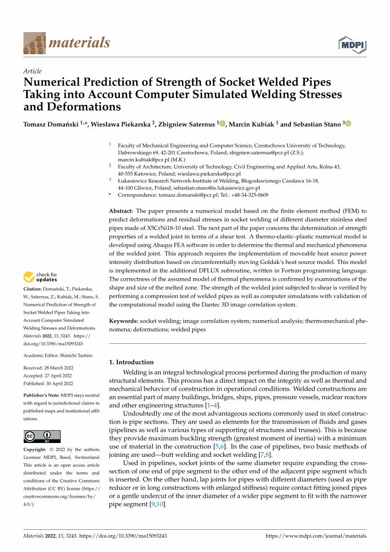
Figure 3. Diagram of surface image analysis before and after deformation [34].

Correlation algorithms make it possible to determine the maximum displacement

with an accuracy of 1/100 of a pixel of the matrix. The correlation algorithm tracks the

position of the same points visible in the source image and the distorted image. To

achieve this, a square surface containing a set of pixels is identified in the source image

and at a position appropriate for the image after deformation.

Figure 4 shows a diagram of the research station, which distinguishes three basic

groups of elements: the tested object (sample with the loading system), the measuring

system and the system analyzing results of the measurement. The measuring system is

equipped with a set of digital cameras mounted on a common tripod. This system is

Figure 2. A circumferentially welded pipe of different diameters: (a) general view, (b) macroscopicview of the cross-section of the weld.

The metallographic tests were performed to determine the size and shape of the meltedzone. The data obtained from experimental tests are necessary in the verification of theheat source power distribution model. The macroscopic picture of welded joint allowedcomparing the shape of the melted zone with the results of the numerical simulations.Accurate determination of the heat load ensured proper temperature distribution in thejoint and appropriate analysis of welding stresses and deformations [19,24].

Materials 2022, 15, 3243 4 of 19


Measuring methods using image correlation are now more and more often used todetermine the components of stresses, strains or displacements in laboratory conditions aswell as to identify defects in construction elements or machines generated during static ordynamic loads [34–38]. The correlation algorithm tracks the position of the same points inthe source image and the distorted image (Figure 3).


Figure 2. A circumferentially welded pipe of different diameters: (a) general view, (b) macroscopic

view of the cross-section of the weld.

The metallographic tests were performed to determine the size and shape of the

melted zone. The data obtained from experimental tests are necessary in the verification

of the heat source power distribution model. The macroscopic picture of welded joint

allowed comparing the shape of the melted zone with the results of the numerical simu-

lations. Accurate determination of the heat load ensured proper temperature distribution

in the joint and appropriate analysis of welding stresses and deformations [19,24].


Measuring methods using image correlation are now more and more often used to

determine the components of stresses, strains or displacements in laboratory conditions

as well as to identify defects in construction elements or machines generated during static

or dynamic loads [34–38]. The correlation algorithm tracks the position of the same points

in the source image and the distorted image (Figure 3).


Correlation algorithms make it possible to determine the maximum displacement

with an accuracy of 1/100 of a pixel of the matrix. The correlation algorithm tracks the

position of the same points visible in the source image and the distorted image. To

achieve this, a square surface containing a set of pixels is identified in the source image

and at a position appropriate for the image after deformation.

Figure 4 shows a diagram of the research station, which distinguishes three basic

groups of elements: the tested object (sample with the loading system), the measuring

system and the system analyzing results of the measurement. The measuring system is

equipped with a set of digital cameras mounted on a common tripod. This system is


Correlation algorithms make it possible to determine the maximum displacement withan accuracy of 1/100 of a pixel of the matrix. The correlation algorithm tracks the positionof the same points visible in the source image and the distorted image. To achieve this, asquare surface containing a set of pixels is identified in the source image and at a positionappropriate for the image after deformation.

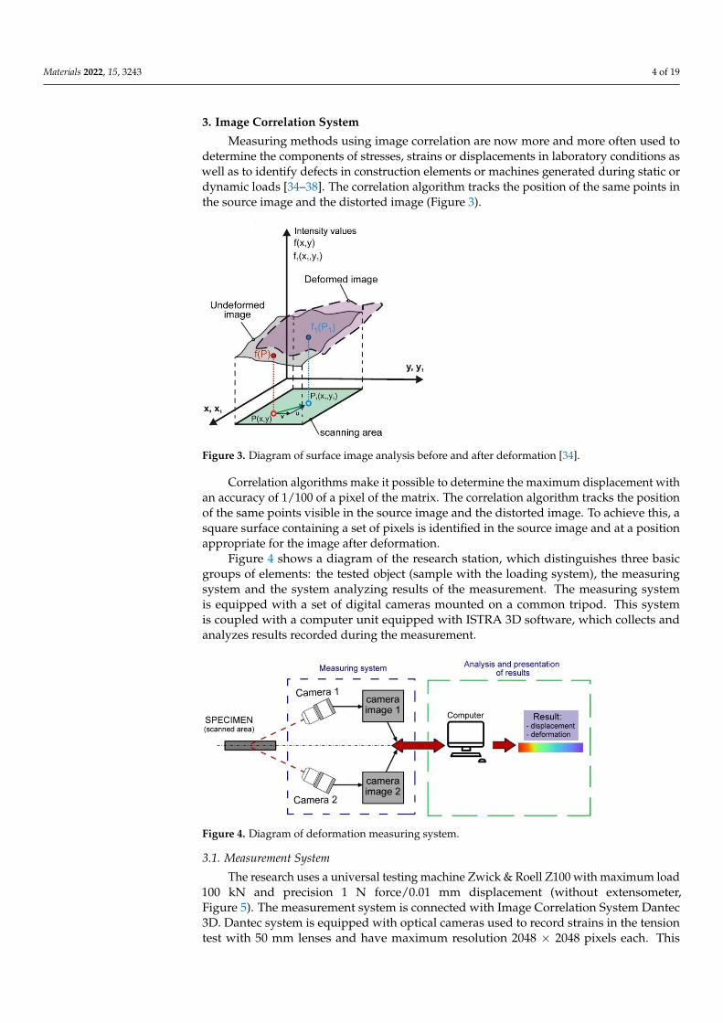
Figure 4 shows a diagram of the research station, which distinguishes three basicgroups of elements: the tested object (sample with the loading system), the measuringsystem and the system analyzing results of the measurement. The measuring systemis equipped with a set of digital cameras mounted on a common tripod. This systemis coupled with a computer unit equipped with ISTRA 3D software, which collects andanalyzes results recorded during the measurement.


coupled with a computer unit equipped with ISTRA 3D software, which collects and an-

alyzes results recorded during the measurement.

Figure 4. Diagram of deformation measuring system.

3.1. Measurement System

The research uses a universal testing machine Zwick & Roell Z100 with maximum

load 100 kN and precision 1 N force/0.01 mm displacement (without extensometer, Fig-

ure 5). The measurement system is connected with Image Correlation System Dantec 3D.

Dantec system is equipped with optical cameras used to record strains in the tension test

with 50 mm lenses and have maximum resolution 2048 × 2048 pixels each. This allowed

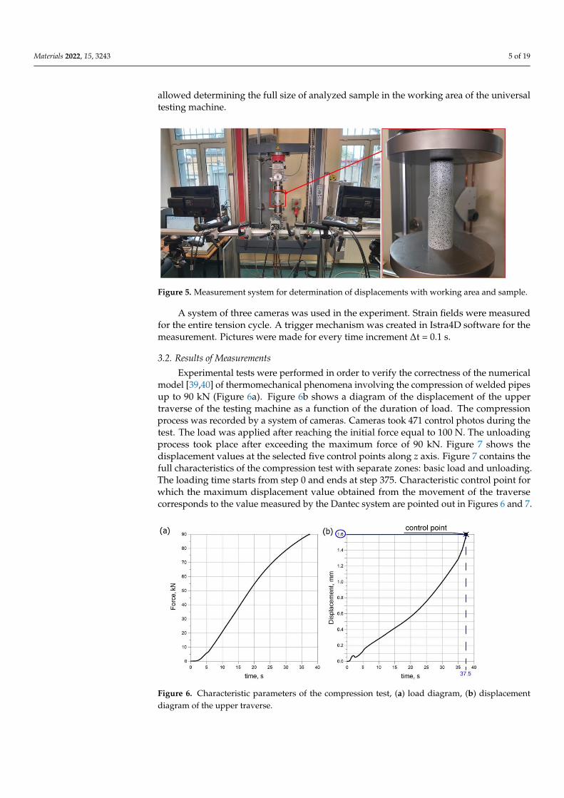
determining the full size of analyzed sample in the working area of the universal testing

machine.

Figure 5. Measurement system for determination of displacements with working area and sample.

A system of three cameras was used in the experiment. Strain fields were measured

for the entire tension cycle. A trigger mechanism was created in Istra4D software for the

measurement. Pictures were made for every time increment Δt = 0.1 s.

3.2. Results of Measurements

Experimental tests were performed in order to verify the correctness of the numer-

ical model [39,40] of thermomechanical phenomena involving the compression of welded

pipes up to 90 kN (Figure 6a). Figure 6b shows a diagram of the displacement of the

upper traverse of the testing machine as a function of the duration of load. The compres-

sion process was recorded by a system of cameras. Cameras took 471 control photos

during the test. The load was applied after reaching the initial force equal to 100 N. The

unloading process took place after exceeding the maximum force of 90 kN. Figure 7

shows the displacement values at the selected five control points along z axis. Figure 7



The research uses a universal testing machine Zwick & Roell Z100 with maximum load100 kN and precision 1 N force/0.01 mm displacement (without extensometer,Figure 5). The measurement system is connected with Image Correlation System Dantec3D. Dantec system is equipped with optical cameras used to record strains in the tensiontest with 50 mm lenses and have maximum resolution 2048 × 2048 pixels each. This

Materials 2022, 15, 3243 5 of 19

allowed determining the full size of analyzed sample in the working area of the universaltesting machine.


coupled with a computer unit equipped with ISTRA 3D software, which collects and an-

alyzes results recorded during the measurement.



The research uses a universal testing machine Zwick & Roell Z100 with maximum

load 100 kN and precision 1 N force/0.01 mm displacement (without extensometer, Fig-

ure 5). The measurement system is connected with Image Correlation System Dantec 3D.

Dantec system is equipped with optical cameras used to record strains in the tension test

with 50 mm lenses and have maximum resolution 2048 × 2048 pixels each. This allowed

determining the full size of analyzed sample in the working area of the universal testing

machine.


A system of three cameras was used in the experiment. Strain fields were measured

for the entire tension cycle. A trigger mechanism was created in Istra4D software for the

measurement. Pictures were made for every time increment Δt = 0.1 s.


Experimental tests were performed in order to verify the correctness of the numer-

ical model [39,40] of thermomechanical phenomena involving the compression of welded

pipes up to 90 kN (Figure 6a). Figure 6b shows a diagram of the displacement of the

upper traverse of the testing machine as a function of the duration of load. The compres-

sion process was recorded by a system of cameras. Cameras took 471 control photos

during the test. The load was applied after reaching the initial force equal to 100 N. The

unloading process took place after exceeding the maximum force of 90 kN. Figure 7

shows the displacement values at the selected five control points along z axis. Figure 7


A system of three cameras was used in the experiment. Strain fields were measuredfor the entire tension cycle. A trigger mechanism was created in Istra4D software for themeasurement. Pictures were made for every time increment ∆t = 0.1 s.


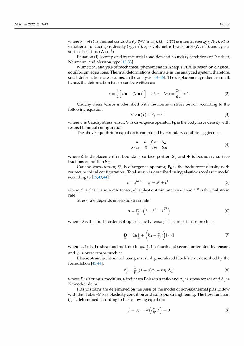
Experimental tests were performed in order to verify the correctness of the numericalmodel [39,40] of thermomechanical phenomena involving the compression of welded pipesup to 90 kN (Figure 6a). Figure 6b shows a diagram of the displacement of the uppertraverse of the testing machine as a function of the duration of load. The compressionprocess was recorded by a system of cameras. Cameras took 471 control photos during thetest. The load was applied after reaching the initial force equal to 100 N. The unloadingprocess took place after exceeding the maximum force of 90 kN. Figure 7 shows thedisplacement values at the selected five control points along z axis. Figure 7 contains thefull characteristics of the compression test with separate zones: basic load and unloading.The loading time starts from step 0 and ends at step 375. Characteristic control point forwhich the maximum displacement value obtained from the movement of the traversecorresponds to the value measured by the Dantec system are pointed out in Figures 6 and 7.


contains the full characteristics of the compression test with separate zones: basic load

and unloading. The loading time starts from step 0 and ends at step 375. Characteristic

control point for which the maximum displacement value obtained from the movement

of the traverse corresponds to the value measured by the Dantec system are pointed out

in Figures 6 and 7.

Figure 6. Characteristic parameters of the compression test, (a) load diagram, (b) displacement

diagram of the upper traverse.

Figure 7. Uz displacement diagram for five selected measuring points.

Figure 8a shows the displacement field along the z axis (the axis compliant with the

loading direction), where the measurement line is marked as a solid line. For this line, the

displacement diagram is shown in Figure 8b. The measuring line is on the side surface of

welded pipes. It can be observed that in the area of the weld; the displacements have

much lower values compared to the base material, which is related to the increase in

stiffness of this area, resulting from the change of mechanical properties of the weld.

Figure 6. Characteristic parameters of the compression test, (a) load diagram, (b) displacementdiagram of the upper traverse.

Materials 2022, 15, 3243 6 of 19


contains the full characteristics of the compression test with separate zones: basic load

and unloading. The loading time starts from step 0 and ends at step 375. Characteristic

control point for which the maximum displacement value obtained from the movement

of the traverse corresponds to the value measured by the Dantec system are pointed out

in Figures 6 and 7.

Figure 6. Characteristic parameters of the compression test, (a) load diagram, (b) displacement

diagram of the upper traverse.


Figure 8a shows the displacement field along the z axis (the axis compliant with the

loading direction), where the measurement line is marked as a solid line. For this line, the

displacement diagram is shown in Figure 8b. The measuring line is on the side surface of

welded pipes. It can be observed that in the area of the weld; the displacements have

much lower values compared to the base material, which is related to the increase in

stiffness of this area, resulting from the change of mechanical properties of the weld.


Figure 8a shows the displacement field along the z axis (the axis compliant with theloading direction), where the measurement line is marked as a solid line. For this line, thedisplacement diagram is shown in Figure 8b. The measuring line is on the side surface ofwelded pipes. It can be observed that in the area of the weld; the displacements have muchlower values compared to the base material, which is related to the increase in stiffness ofthis area, resulting from the change of mechanical properties of the weld.


Figure 8. Experimental displacement distribution in the z axis (a) on the outer surface, (b) along the

center lines.

The displacement distribution Ux, Uy over time 37.5 s (which corresponds to the ac-

tion of specific load) on the side surface of the pipes is shown in Figure 9. The visible

decrease in the value of the displacement occurs within the weld in the perpendicular

direction to the side surface (axis y). A slight increase in the displacements along the x

axis (horizontal) is caused by a small deflection of the sample caused by a low slip of the

pressure plate.

Figure 8. Experimental displacement distribution in the z axis (a) on the outer surface, (b) along thecenter lines.

Materials 2022, 15, 3243 7 of 19

The displacement distribution Ux, Uy over time 37.5 s (which corresponds to the actionof specific load) on the side surface of the pipes is shown in Figure 9. The visible decreasein the value of the displacement occurs within the weld in the perpendicular direction tothe side surface (axis y). A slight increase in the displacements along the x axis (horizontal)is caused by a small deflection of the sample caused by a low slip of the pressure plate.

Figure 9. Displacement (a) in the x axis, (b) in the y axis.

4. Mathematical and Numerical Modeling of Circumferential Welding of Pipes4.1. Mathematical Models of Thermomechanical Phenomena

Numerical analysis of thermomechanical phenomena is divided into thermal andmechanical analysis [19,41,42].

Thermal phenomena are described by a heat transfer equation in the Abaqus/Standardsimulation module. The solution equation is based on the law of energy conservation andFourier’s law [27]. This equation is described by the following formula:∫

V

ρ∂U∂t

δTdV +∫V

∂δT∂xα·(

λ∂T∂xα

)dV ==

∫V

δT qVdV +∫S

δT qSdS (1)

Materials 2022, 15, 3243 8 of 19

where λ = λ(T) is thermal conductivity (W/(m K)), U = U(T) is internal energy (J/kg), δT isvariational function, ρ is density (kg/m3), qv is volumetric heat source (W/m3), and qS is asurface heat flux (W/m2).

Equation (1) is completed by the initial condition and boundary conditions of Dirichlet,Neumann, and Newton type [19,33].

Numerical analysis of mechanical phenomena in Abaqus FEA is based on classicalequilibrium equations. Thermal deformations dominate in the analyzed system; therefore,small deformations are assumed in the analysis [43–45]. The displacement gradient is small;hence, the deformation tensor can be written as:

ε =12

[∇u + (∇u)T

]when ∇u =

∂u∂u≈ 1 (2)

Cauchy stress tensor is identified with the nominal stress tensor, according to thefollowing equation:

∇ ◦σ(x) + Fb = 0 (3)

where σ is Cauchy stress tensor,∇ is divergence operator, Fb is the body force density withrespect to initial configuration.

The above equilibrium equation is completed by boundary conditions, given as:

u = u f or Suσ · n = Φ f or SΦ

(4)

where û is displacement on boundary surface portion Su and Φ is boundary surfacetractions on portion SΦ.

Cauchy stress tensor, ∇, is divergence operator, Fb is the body force density withrespect to initial configuration. Total strain is described using elastic–iscoplastic modelaccording to [19,43,44]:

ε = εtotal = εe + εp + εTh (5)

where εe is elastic strain rate tensor, εp is plastic strain rate tensor and εTh is thermal strainrate.

Stress rate depends on elastic strain rate

.σ = D

=:( .ε− .

εp − .

εTh)

(6)

where D=

is the fourth order isotropic elasticity tensor, “:” is inner tensor product.

D== 2µ I

=+

(kB −

23

µ

)I⊗ I (7)

where µ, kB is the shear and bulk modulus, I=

, I is fourth and second order identity tensors

and ⊗ is outer tensor product.Elastic strain is calculated using inverted generalized Hook’s law, described by the

formulation [43,44]:

εeij =

1E[(1 + υ)σij − υσkkδij

](8)

where E is Young’s modulus, ν indicates Poisson’s ratio and σij is stress tensor and δij isKronecker delta.

Plastic strains are determined on the basis of the model of non-isothermal plastic flowwith the Huber–Mises plasticity condition and isotropic strengthening. The flow function(f ) is determined according to the following equation:

f = σe f − σ(

εpij, T

)= 0 (9)

Materials 2022, 15, 3243 9 of 19

where σe f is effective stress, σ(

εpij, T

)is material plasticizing stress—dependent on plastic

deformation (εpij) and temperature T.

Effective stress and strain are described as follows:

σe f =

√32

SijSij and.ε

pe f =

√23

.ε

pij

.ε

pij (10)

where Sij is a deviatoric stress tensor (Sij = σij − 13 σmδij), σm is an average stress.

The plastic deformation rate can be expressed in the following form

.ε

pij =

32

.ε

pe f

Sij

σe f(11)

where.ε

plij is plastic strain rate component, λ signifies the plastic flow factor and Sij represents

the deviatoric stress.Thermal strain occurs as a result of changes in volume due to temperature differences:

εThij =

T∫T0

α(T)dTδij (12)

where α is the temperature-dependent coefficient of thermal expansion, T0 is the referencetemperature.

4.2. Modelling of the Heat Source

In the case of numerical modeling of the electric arc-welding process, the Goldak modelis most often used in the literature to describe the source power distribution [33,46,47].This model is described by two half ellipsoids connected together by a symmetry axis [46].The model diagram is shown in Figure 10. The equation describing Goldak’s model isexpressed in the following equation:

Q1(x, y, z) = 6√

3 f1QAabc1π

√π

exp(−3 x2

c12 ) exp(−3 z2

a2 ) exp(−3 y2

b2 )

Q2(x, y, z) = 6√

3 f2QAabc2π

√π

exp(−3 x2

c22 ) exp(−3 z2

a2 ) exp(−3 y2

b2 )(13)

where parameters a, b, c1 and c2 are described dimensions of shape’s Goldak heat source,coefficients f 1 representing energy distribution in the front of the heat source and coefficientsf 2 representing energy distribution in the back of the heat source, (f 1 + f 2 = 2), satisfyingthe condition Q1(x,y,z) and Q2(x,y,z).


ef

ijp

ef

p

ij

S

2

3

(11)

where pl

ij is plastic strain rate component, λ signifies the plastic flow factor and Sij rep-

resents the deviatoric stress.

Thermal strain occurs as a result of changes in volume due to temperature differ-

ences:

T

T

ij

Th

ijdTT

0

)(

(12)

where α is the temperature-dependent coefficient of thermal expansion, T0 is the refer-

ence temperature.

4.2. Modelling of the Heat Source

In the case of numerical modeling of the electric arc-welding process, the Goldak

model is most often used in the literature to describe the source power distribution

[33,46,47]. This model is described by two half ellipsoids connected together by a sym-

metry axis [46]. The model diagram is shown in Figure 10. The equation describing

Goldak’s model is expressed in the following equation:

)3exp()3exp()3exp(36

),,(

)3exp()3exp()3exp(36

),,(

2

2

2

2

2

2

2

2

22

2

2

2

2

2

1

2

1

11

b

y

a

z

c

x

abc

QfzyxQ

b

y

a

z

c

x

abc

QfzyxQ

A

A

(13)

where parameters a, b, c1 and c2 are described dimensions of shape’s Goldak heat source,

coefficients f1 representing energy distribution in the front of the heat source and coeffi-

cients f2 representing energy distribution in the back of the heat source, (f1 + f2 = 2), satis-

fying the condition Q1(x,y,z) and Q2(x,y,z).

In Equation (13) parameter QA describes the value of the electric arc power:

UIQA (14)

where U is voltage [V], I is current intensity [A] and η is the efficiency.

Figure 10. Scheme of Goldak’s model (Equation (13)).

Additional subroutine DEFLUX is implemented into Abaqus FEA solver to define a

moveable welding source [19,33]. The subroutine includes a mathematical model of the

distribution of heat source power, speed and direction of source travel. The main aspect

Figure 10. Scheme of Goldak’s model (Equation (13)).

In Equation (13) parameter QA describes the value of the electric arc power:

QA = I ·U · η (14)

Materials 2022, 15, 3243 10 of 19

where U is voltage [V], I is current intensity [A] and η is the efficiency.Additional subroutine DEFLUX is implemented into Abaqus FEA solver to define a

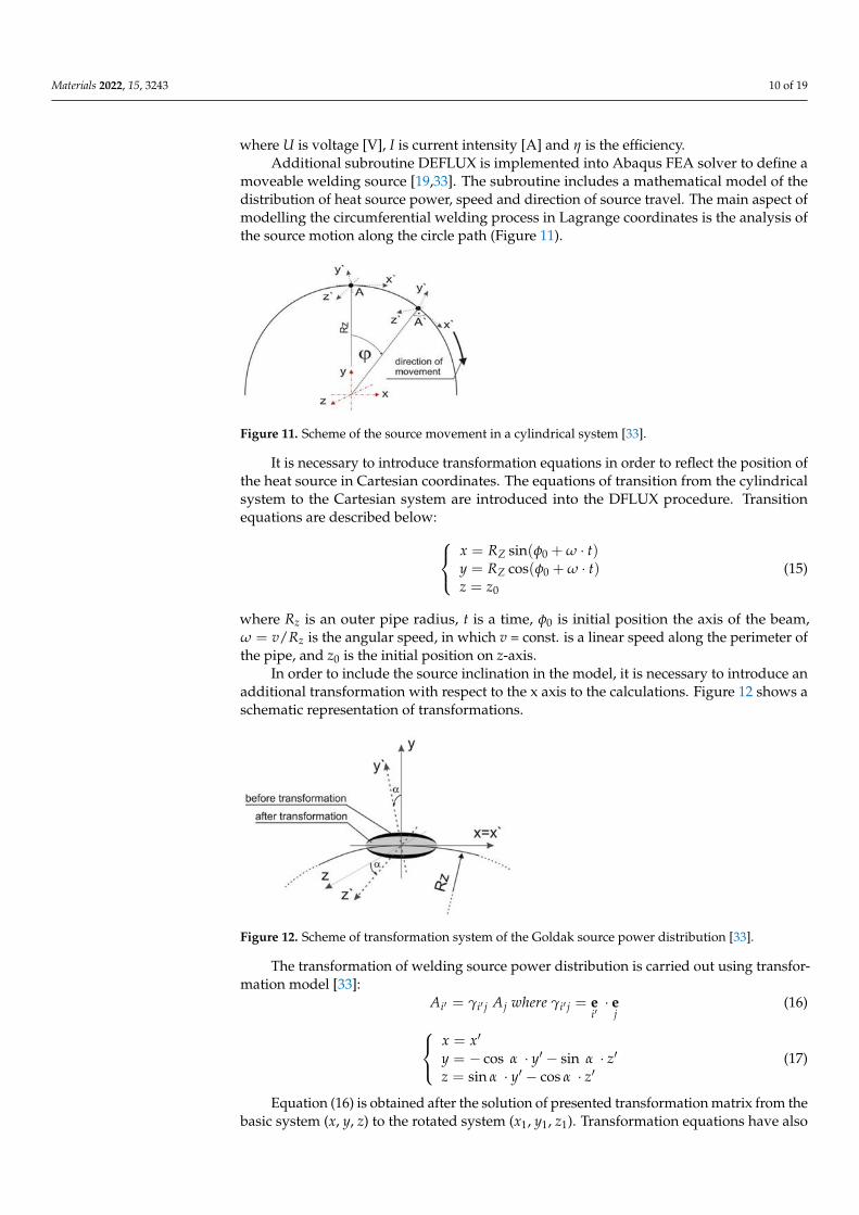
moveable welding source [19,33]. The subroutine includes a mathematical model of thedistribution of heat source power, speed and direction of source travel. The main aspect ofmodelling the circumferential welding process in Lagrange coordinates is the analysis ofthe source motion along the circle path (Figure 11).


of modelling the circumferential welding process in Lagrange coordinates is the analysis

of the source motion along the circle path (Figure 11).

Figure 11. Scheme of the source movement in a cylindrical system [33].

It is necessary to introduce transformation equations in order to reflect the position

of the heat source in Cartesian coordinates. The equations of transition from the cylin-

drical system to the Cartesian system are introduced into the DFLUX procedure. Transi-

tion equations are described below:

0

0

0

)cos(

)sin(

zz

tRy

tRx

Z

Z

(15)

where Rz is an outer pipe radius, t is a time, 0 is initial position the axis of the beam,

zRv / is the angular speed, in which v = const. is a linear speed along the perimeter

of the pipe, and z0 is the initial position on z-axis.

In order to include the source inclination in the model, it is necessary to introduce an

additional transformation with respect to the x axis to the calculations. Figure 12 shows a

schematic representation of transformations.

Figure 12. Scheme of transformation system of the Goldak source power distribution [33].

The transformation of welding source power distribution is carried out using

transformation model [33]:

jijijjii whereAA ee

(16)

zyz

zyy

xx

cossin

sincos

(17)

Equation (16) is obtained after the solution of presented transformation matrix from

the basic system (x, y, z) to the rotated system (x1, y1, z1). Transformation equations have


It is necessary to introduce transformation equations in order to reflect the position ofthe heat source in Cartesian coordinates. The equations of transition from the cylindricalsystem to the Cartesian system are introduced into the DFLUX procedure. Transitionequations are described below:

x = RZ sin(φ0 + ω · t)y = RZ cos(φ0 + ω · t)z = z0

(15)

where Rz is an outer pipe radius, t is a time, φ0 is initial position the axis of the beam,ω = v/Rz is the angular speed, in which v = const. is a linear speed along the perimeter ofthe pipe, and z0 is the initial position on z-axis.

In order to include the source inclination in the model, it is necessary to introduce anadditional transformation with respect to the x axis to the calculations. Figure 12 shows aschematic representation of transformations.


of modelling the circumferential welding process in Lagrange coordinates is the analysis

of the source motion along the circle path (Figure 11).


It is necessary to introduce transformation equations in order to reflect the position

of the heat source in Cartesian coordinates. The equations of transition from the cylin-

drical system to the Cartesian system are introduced into the DFLUX procedure. Transi-

tion equations are described below:

0

0

0

)cos(

)sin(

zz

tRy

tRx

Z

Z

(15)

where Rz is an outer pipe radius, t is a time, 0 is initial position the axis of the beam,

zRv / is the angular speed, in which v = const. is a linear speed along the perimeter

of the pipe, and z0 is the initial position on z-axis.

In order to include the source inclination in the model, it is necessary to introduce an

additional transformation with respect to the x axis to the calculations. Figure 12 shows a

schematic representation of transformations.


The transformation of welding source power distribution is carried out using

transformation model [33]:

jijijjii whereAA ee

(16)

zyz

zyy

xx

cossin

sincos

(17)

Equation (16) is obtained after the solution of presented transformation matrix from

the basic system (x, y, z) to the rotated system (x1, y1, z1). Transformation equations have


The transformation of welding source power distribution is carried out using transfor-mation model [33]:

Ai′ = γi′ j Aj where γi′ j = ei′· e

j(16)

x = x′

y = − cos α · y′ − sin α · z′z = sin α · y′ − cos α · z′

(17)

Equation (16) is obtained after the solution of presented transformation matrix from thebasic system (x, y, z) to the rotated system (x1, y1, z1). Transformation equations have also

Materials 2022, 15, 3243 11 of 19

been written in the DFLUX subroutine. Numerical modelling of circumferential welding oftwo pipes of different diameters also requires the appropriate angle of inclination of theheat source axis. Figure 13 shows the inclination of heat source adopted in the model. Theaxis of the welding source is rotated by an angle α = 20◦ (the inclination direction is thesame as in the experiment).


also been written in the DFLUX subroutine. Numerical modelling of circumferential

welding of two pipes of different diameters also requires the appropriate angle of incli-

nation of the heat source axis. Figure 13 shows the inclination of heat source adopted in

the model. The axis of the welding source is rotated by an angle α = 20° (the inclination

direction is the same as in the experiment).

Figure 13. Scheme of the inclination of the heat source.

4.3. Numerical Model

The numerical model in Abaqus FEA is developed using the real welded pipes

(shown in Figure 1). The model of geometry of the welded pipes is presented in Figure 14

with the finite element mesh.

Figure 14. Discrete model of the analyzed joint.

The smaller FE-mesh step is about 0.25 mm and it occurs in the heat source activity

zone. The total number of finite elements is 495,100. The material model of steel

X5CrNi18-10 is assumed from literature data [32,33] as: solidus and liquidus tempera-

tures TS = 1400 °C, TL = 1455 °C, latent heat of fusion HL = 260 × 103 J/kg, ambient temper-

ature T0 = 20 °C and the heat convection αk = 50 W/m2.

The basic parameters of Goldak’s source are assumed using data from the experi-

ment. The power of the heat source is determined on the basis of Equation (13) with QA =

996 W (assuming the efficiency of the process η = 60%). Welding speed is set to v = 0.3

[m/min], and the angle of deflection of the welding torch from the vertical plane is set to

20°. On the basis of numerical verification, the following parameters of Goldak’s source

are assumed: a = 4 mm, b = 2 mm, c1 = 4 mm and c2 = 4 mm. Coefficients are f1 = 1 and f2 = 1

(f1 + f2 = 2).

During the analysis of thermal phenomena, perfect contact between the joined ele-

ments is considered. In the case of the analysis of mechanical phenomena, „self-contact”

[40] between the inner plane of pipe with a larger diameter and the outer plane of pipe

with a smaller diameter is assumed. Figure 15 shows the location of the self-contact.



The numerical model in Abaqus FEA is developed using the real welded pipes (shownin Figure 1). The model of geometry of the welded pipes is presented in Figure 14 with thefinite element mesh.


also been written in the DFLUX subroutine. Numerical modelling of circumferential

welding of two pipes of different diameters also requires the appropriate angle of incli-

nation of the heat source axis. Figure 13 shows the inclination of heat source adopted in

the model. The axis of the welding source is rotated by an angle α = 20° (the inclination

direction is the same as in the experiment).



The numerical model in Abaqus FEA is developed using the real welded pipes

(shown in Figure 1). The model of geometry of the welded pipes is presented in Figure 14

with the finite element mesh.


The smaller FE-mesh step is about 0.25 mm and it occurs in the heat source activity

zone. The total number of finite elements is 495,100. The material model of steel

X5CrNi18-10 is assumed from literature data [32,33] as: solidus and liquidus tempera-

tures TS = 1400 °C, TL = 1455 °C, latent heat of fusion HL = 260 × 103 J/kg, ambient temper-

ature T0 = 20 °C and the heat convection αk = 50 W/m2.

The basic parameters of Goldak’s source are assumed using data from the experi-

ment. The power of the heat source is determined on the basis of Equation (13) with QA =

996 W (assuming the efficiency of the process η = 60%). Welding speed is set to v = 0.3

[m/min], and the angle of deflection of the welding torch from the vertical plane is set to

20°. On the basis of numerical verification, the following parameters of Goldak’s source

are assumed: a = 4 mm, b = 2 mm, c1 = 4 mm and c2 = 4 mm. Coefficients are f1 = 1 and f2 = 1

(f1 + f2 = 2).

During the analysis of thermal phenomena, perfect contact between the joined ele-

ments is considered. In the case of the analysis of mechanical phenomena, „self-contact”

[40] between the inner plane of pipe with a larger diameter and the outer plane of pipe

with a smaller diameter is assumed. Figure 15 shows the location of the self-contact.


The smaller FE-mesh step is about 0.25 mm and it occurs in the heat source activ-ity zone. The total number of finite elements is 495,100. The material model of steelX5CrNi18-10 is assumed from literature data [32,33] as: solidus and liquidus temperaturesTS = 1400 ◦C, TL = 1455 ◦C, latent heat of fusion HL = 260 × 103 J/kg, ambient temperatureT0 = 20 ◦C and the heat convection αk = 50 W/m2.

The basic parameters of Goldak’s source are assumed using data from the experiment.The power of the heat source is determined on the basis of Equation (13) with QA = 996 W(assuming the efficiency of the process η = 60%). Welding speed is set to v = 0.3 [m/min],and the angle of deflection of the welding torch from the vertical plane is set to 20◦. On thebasis of numerical verification, the following parameters of Goldak’s source are assumed: a= 4 mm, b = 2 mm, c1 = 4 mm and c2 = 4 mm. Coefficients are f 1 = 1 and f 2 = 1 (f 1 + f 2 = 2).

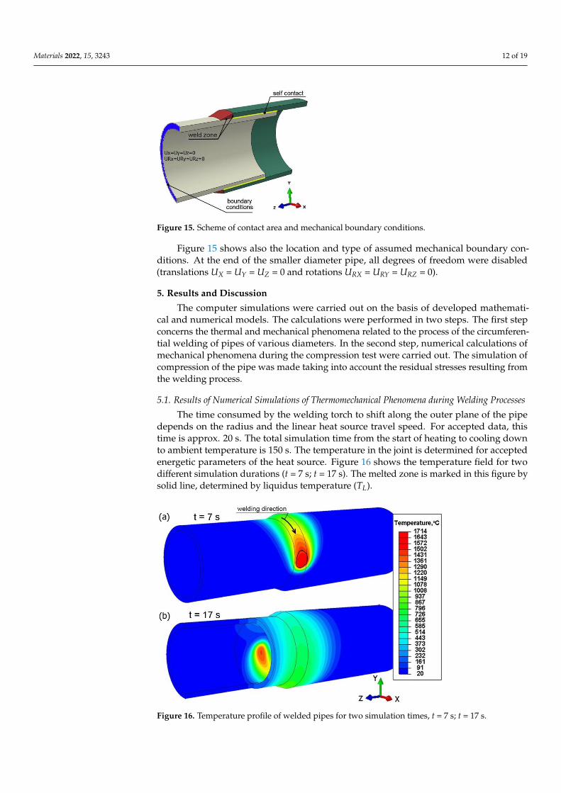
During the analysis of thermal phenomena, perfect contact between the joined ele-ments is considered. In the case of the analysis of mechanical phenomena, “self-contact” [40]between the inner plane of pipe with a larger diameter and the outer plane of pipe with asmaller diameter is assumed. Figure 15 shows the location of the self-contact.

Materials 2022, 15, 3243 12 of 19Materials 2022, 15, x FOR PEER REVIEW 13 of 20

Figure 15. Scheme of contact area and mechanical boundary conditions.

Figure 15 shows also the location and type of assumed mechanical boundary condi-

tions. At the end of the smaller diameter pipe, all degrees of freedom were disabled

(translations UX = UY = UZ = 0 and rotations URX = URY = URZ = 0).

5. Results and Discussion

The computer simulations were carried out on the basis of developed mathematical

and numerical models. The calculations were performed in two steps. The first step

concerns the thermal and mechanical phenomena related to the process of the circum-

ferential welding of pipes of various diameters. In the second step, numerical calculations

of mechanical phenomena during the compression test were carried out. The simulation

of compression of the pipe was made taking into account the residual stresses resulting

from the welding process.

Figure 15. Scheme of contact area and mechanical boundary conditions.

Figure 15 shows also the location and type of assumed mechanical boundary con-ditions. At the end of the smaller diameter pipe, all degrees of freedom were disabled(translations UX = UY = UZ = 0 and rotations URX = URY = URZ = 0).

5. Results and Discussion

The computer simulations were carried out on the basis of developed mathemati-cal and numerical models. The calculations were performed in two steps. The first stepconcerns the thermal and mechanical phenomena related to the process of the circumferen-tial welding of pipes of various diameters. In the second step, numerical calculations ofmechanical phenomena during the compression test were carried out. The simulation ofcompression of the pipe was made taking into account the residual stresses resulting fromthe welding process.

5.1. Results of Numerical Simulations of Thermomechanical Phenomena during Welding Processes

The time consumed by the welding torch to shift along the outer plane of the pipedepends on the radius and the linear heat source travel speed. For accepted data, thistime is approx. 20 s. The total simulation time from the start of heating to cooling downto ambient temperature is 150 s. The temperature in the joint is determined for acceptedenergetic parameters of the heat source. Figure 16 shows the temperature field for twodifferent simulation durations (t = 7 s; t = 17 s). The melted zone is marked in this figure bysolid line, determined by liquidus temperature (TL).


5.1. Results of Numerical Simulations of Thermomechanical Phenomena during Welding Pro-

cesses

The time consumed by the welding torch to shift along the outer plane of the pipe

depends on the radius and the linear heat source travel speed. For accepted data, this

time is approx. 20 s. The total simulation time from the start of heating to cooling down to

ambient temperature is 150 s. The temperature in the joint is determined for accepted

energetic parameters of the heat source. Figure 16 shows the temperature field for two

different simulation durations (t = 7 s; t = 17 s). The melted zone is marked in this figure

by solid line, determined by liquidus temperature (TL).

Figure 16. Temperature profile of welded pipes for two simulation times, t = 7 s; t = 17 s.

Figure 17a shows the temperature field in the cross-section of the joint for time t = 10

s. The solid line marks the boundary of the melted zone. The results of the simulation of

temperature distribution were verified experimentally. Figure 17b shows a cross-section

of the real weld where the boundary of the melted zone (the solid line marks the range of

the melted zone, TL ≈ 1455 °C) is given in the frame. As can be observed, for assumptions

accepted in the model, a good agreement of the results is obtained.

Figure 17. Cross-section of the joint (a) results of numerical calculations, (b) real weld.

The numerically determined thermal load acting on the combined system of two

pipes of different diameters allowed performing calculations of mechanical phenomena.

Figure 18 shows the distribution of temporary reduced stress for two different simulation

times, t = 8 s and t = 17 s. The largest temporary stresses occur in the area of heating


Materials 2022, 15, 3243 13 of 19

Figure 17a shows the temperature field in the cross-section of the joint for time t = 10 s.The solid line marks the boundary of the melted zone. The results of the simulation oftemperature distribution were verified experimentally. Figure 17b shows a cross-sectionof the real weld where the boundary of the melted zone (the solid line marks the range ofthe melted zone, TL ≈ 1455 ◦C) is given in the frame. As can be observed, for assumptionsaccepted in the model, a good agreement of the results is obtained.


5.1. Results of Numerical Simulations of Thermomechanical Phenomena during Welding Pro-

cesses

The time consumed by the welding torch to shift along the outer plane of the pipe

depends on the radius and the linear heat source travel speed. For accepted data, this

time is approx. 20 s. The total simulation time from the start of heating to cooling down to

ambient temperature is 150 s. The temperature in the joint is determined for accepted

energetic parameters of the heat source. Figure 16 shows the temperature field for two

different simulation durations (t = 7 s; t = 17 s). The melted zone is marked in this figure

by solid line, determined by liquidus temperature (TL).


Figure 17a shows the temperature field in the cross-section of the joint for time t = 10

s. The solid line marks the boundary of the melted zone. The results of the simulation of

temperature distribution were verified experimentally. Figure 17b shows a cross-section

of the real weld where the boundary of the melted zone (the solid line marks the range of

the melted zone, TL ≈ 1455 °C) is given in the frame. As can be observed, for assumptions

accepted in the model, a good agreement of the results is obtained.


The numerically determined thermal load acting on the combined system of two

pipes of different diameters allowed performing calculations of mechanical phenomena.

Figure 18 shows the distribution of temporary reduced stress for two different simulation

times, t = 8 s and t = 17 s. The largest temporary stresses occur in the area of heating


The numerically determined thermal load acting on the combined system of twopipes of different diameters allowed performing calculations of mechanical phenomena.Figure 18 shows the distribution of temporary reduced stress for two different simulationtimes, t = 8 s and t = 17 s. The largest temporary stresses occur in the area of heating sourceaction on the material with the amount of 255 MPa. Residual reduced stress after cooling toambient temperature is presented in Figure 19 for time t = 150 s.


source action on the material with the amount of 255 MPa. Residual reduced stress after

cooling to ambient temperature is presented in Figure 19 for time t = 150 s.

From the comparison of Figures 18 and 19, it can be seen that after lowering the joint

temperature to the ambient temperature (t = 150 s), the maximum stresses decreased.

Figure 18. Temporary reduced stresses of a welded joint for two different simulation times, t = 8 s; t

= 17 s.

Figure 19. Reduced stresses after welding, for time t = 150 s.

The displacement field of the welded joint is numerically predicted. Figure 20 shows

the displacement field in a general view (Uz, Uy, Uz). For the analyzed welded system of

two pipes, the highest value of displacements is approx. 0.03 cm (0.3 mm).

For the assumed mechanical boundary conditions, the highest values of displace-

ments are directed along the z axis (Uz, Figure 20c) in the analyzed joint. On the basis of

results shown in Figure 20a,b, it can be seen that the cross-section of the joint is deformed

due to the operation of the welding source. The displacement values in the direction of

the x and y axes are comparable with the approximate amount of 0.2 mm.

Figure 18. Temporary reduced stresses of a welded joint for two different simulation times, t = 8 s;t = 17 s.

Materials 2022, 15, 3243 14 of 19


source action on the material with the amount of 255 MPa. Residual reduced stress after

cooling to ambient temperature is presented in Figure 19 for time t = 150 s.

From the comparison of Figures 18 and 19, it can be seen that after lowering the joint

temperature to the ambient temperature (t = 150 s), the maximum stresses decreased.

Figure 18. Temporary reduced stresses of a welded joint for two different simulation times, t = 8 s; t

= 17 s.


The displacement field of the welded joint is numerically predicted. Figure 20 shows

the displacement field in a general view (Uz, Uy, Uz). For the analyzed welded system of

two pipes, the highest value of displacements is approx. 0.03 cm (0.3 mm).

For the assumed mechanical boundary conditions, the highest values of displace-

ments are directed along the z axis (Uz, Figure 20c) in the analyzed joint. On the basis of

results shown in Figure 20a,b, it can be seen that the cross-section of the joint is deformed

due to the operation of the welding source. The displacement values in the direction of

the x and y axes are comparable with the approximate amount of 0.2 mm.


From the comparison of Figures 18 and 19, it can be seen that after lowering the jointtemperature to the ambient temperature (t = 150 s), the maximum stresses decreased.

The displacement field of the welded joint is numerically predicted. Figure 20 showsthe displacement field in a general view (Uz, Uy, Uz). For the analyzed welded system oftwo pipes, the highest value of displacements is approx. 0.03 cm (0.3 mm).


Figure 20. Displacement field in welded pipes.

The analyzed method of welding of pipes can be used for various types of con-

struction support. Therefore, it is necessary to carry out a strength analysis such as a

compression test to define mechanical properties of this type of welded construction.

5.2. Results of Numerical Simulations of Compression Tests

In this work, a numerical model of the compression test was developed on the basis

of experimental tests performed using the universal materials testing machine and image

correlation system (see Section 3.1). The strength analysis of the joined pipes was carried

out in the numerical simulations. Adopted in the calculations, a discrete model is shown

in Figure 14.

The sample was loaded by compression forces as shown in the load diagram (Figure

6). The boundary conditions were assumed in accordance with the existing conditions

during the experiment. Boundary conditions assumed in the analysis are shown in Figure

21.

All translational and rotational degrees of freedom are received on the lower surface

of the sample, at the point of contact of the sample with the lower stationary compression

base: Ux = Uy = Uz = 0, URx = URy = URz = 0 and URx = URy = URz = 0. On the other hand, on the

upper contact surface with the movable crossbeam, motion along the z axis is allowed (Ux

= Uy = 0 and URx = URy = URz = 0). The calculations are carried out in the elastic-plastic

range. Material data in the plastic range for X5CrNi18-10 steel are assumed with respect

to literature data [48].

Figure 20. Displacement field in welded pipes.

For the assumed mechanical boundary conditions, the highest values of displacementsare directed along the z axis (Uz, Figure 20c) in the analyzed joint. On the basis of resultsshown in Figure 20a,b, it can be seen that the cross-section of the joint is deformed due tothe operation of the welding source. The displacement values in the direction of the x andy axes are comparable with the approximate amount of 0.2 mm.

Materials 2022, 15, 3243 15 of 19

The analyzed method of welding of pipes can be used for various types of constructionsupport. Therefore, it is necessary to carry out a strength analysis such as a compressiontest to define mechanical properties of this type of welded construction.

5.2. Results of Numerical Simulations of Compression Tests

In this work, a numerical model of the compression test was developed on the basisof experimental tests performed using the universal materials testing machine and imagecorrelation system (see Section 3.1). The strength analysis of the joined pipes was carriedout in the numerical simulations. Adopted in the calculations, a discrete model is shown inFigure 14.

The sample was loaded by compression forces as shown in the load diagram (Figure 6).The boundary conditions were assumed in accordance with the existing conditions duringthe experiment. Boundary conditions assumed in the analysis are shown in Figure 21.


Figure 21. Diagram of the analyzed system during compression test.

Numerical calculations were carried out taking into account the residual stresses

generated in the welding process. The numerically estimated residual stress field (Figure

19) was implemented in the calculations as the initial condition. Stress distribution re-

sulting from the axial compression of the sample was numerically estimated (Figure 22)

as well as the displacement distribution (Figure 23).

Figure 22a shows the distribution of reduced stresses in the first second of the sim-

ulation (t = 1 s). On the other hand, Figure 22b shows the stress distribution for the

maximum compressive force load on the sample (t = 37.5 s).

Figure 22. Distribution of reduced stresses in the compressed sample for time (a) t = 1 s, (b) t = 37.5

s.

From the analysis of the prediction of stress state in the compressed sample (Figure

22), it can be seen that in the initial stage of loading, the highest stress concentration is

located in the welded joint, which is related to the residual stresses from the welding

process. The reduced stresses increase in the entire element during loading with the

compressive force. At maximum load, the maximum stress values occur in the weld zone

(Figure 22b). At the given load of 90 kN, the element is not damaged. However, a further

increase in the load could lead to the destruction of the specimen due to a crack in the


All translational and rotational degrees of freedom are received on the lower surfaceof the sample, at the point of contact of the sample with the lower stationary compressionbase: Ux = Uy = Uz = 0, URx = URy = URz = 0 and URx = URy = URz = 0. On the other hand, onthe upper contact surface with the movable crossbeam, motion along the z axis is allowed(Ux = Uy = 0 and URx = URy = URz = 0). The calculations are carried out in the elastic-plasticrange. Material data in the plastic range for X5CrNi18-10 steel are assumed with respect toliterature data [48].

Numerical calculations were carried out taking into account the residual stressesgenerated in the welding process. The numerically estimated residual stress field (Figure 19)was implemented in the calculations as the initial condition. Stress distribution resultingfrom the axial compression of the sample was numerically estimated (Figure 22) as well asthe displacement distribution (Figure 23).

Materials 2022, 15, 3243 16 of 19



Numerical calculations were carried out taking into account the residual stresses

generated in the welding process. The numerically estimated residual stress field (Figure

19) was implemented in the calculations as the initial condition. Stress distribution re-

sulting from the axial compression of the sample was numerically estimated (Figure 22)

as well as the displacement distribution (Figure 23).

Figure 22a shows the distribution of reduced stresses in the first second of the sim-

ulation (t = 1 s). On the other hand, Figure 22b shows the stress distribution for the

maximum compressive force load on the sample (t = 37.5 s).

Figure 22. Distribution of reduced stresses in the compressed sample for time (a) t = 1 s, (b) t = 37.5

s.

From the analysis of the prediction of stress state in the compressed sample (Figure

22), it can be seen that in the initial stage of loading, the highest stress concentration is

located in the welded joint, which is related to the residual stresses from the welding

process. The reduced stresses increase in the entire element during loading with the

compressive force. At maximum load, the maximum stress values occur in the weld zone

(Figure 22b). At the given load of 90 kN, the element is not damaged. However, a further

increase in the load could lead to the destruction of the specimen due to a crack in the

Figure 22. Distribution of reduced stresses in the compressed sample for time (a) t = 1 s, (b) t = 37.5 s.


weld. Figure 23 shows the displacement distributions taking into account the reduced

residual stresses resulting from welding process.

Figure 23. Displacement fields in the compressed sample: (a) Ux, (b) Uy, (c) Uz and (d) comparison

of Uz displacement with experimental test.

The assumed parameters of the compression test are the same as parameters ob-

tained in the experiment (Figure 6). Therefore, values of longitudinal displacements Uz

are consistent with the experiment. The maximum value of this displacement is up to 1.6

mm (the check point refers to the value of the displacement from the testing machine for

the test time of 37.5 s). The negative sign of the displacement along the z axis direction

results from the adopted coordinate system. This direction of the z axis is opposite to the

direction in the coordinate system found in experimental studies. The obtained dis-

placements in the pipe axis are comparable; their maximum values oscillate around 0.2

mm. Numerically estimated values of displacements in the x axis and y axis are compa-

rable with results of the experiment obtained by the Dantec 3D system (Figure 9). Figure

23d shows a comparison of displacements along the z axis for the measurement line

(Figure 23c) with the results obtained in the Dantec 3D system (Figure 8). A high con-

vergence of the obtained results can be observed in this figure.

6. Conclusions

Contrary to most of the papers on modeling the welding process, this work simu-

lates the thermomechanical phenomena in welding and tests performed to determine the

mechanical properties of the welded construction. Numerical analysis of the welding

process as well as the simulation of mechanical loads during compression tests allowed

the prediction the strength of the joint.

The comparison of numerically estimated liquidus temperature with the results of

the experiment shows that the estimated fusion zone well agrees with the boundary of

the melted zone in the cross-section of the obtained joint. The reduced welding stresses

obtained in the simulations do not exceed the value of 250 MPa and the displacement

values do not exceed 0.3 mm. The obtained simulation results of the welding process are

used as input data for the strength analysis during the compression test of welded pipes.

The experimental results obtained from the Dantec 3D image correlation system are

consistent both in the transverse direction and along the z axis. The comparison of dis-

placement fields in each direction confirmed the correctness of the developed numerical

models.

On the basis of the obtained results of simulation of stresses in the compressed

sample (see Figure 22), it can be seen that in the initial stage of loading, the highest stress

concentration is located in the joint, which is related to the residual welding stresses.

Figure 23. Displacement fields in the compressed sample: (a) Ux, (b) Uy, (c) Uz and (d) comparisonof Uz displacement with experimental test.

Figure 22a shows the distribution of reduced stresses in the first second of the simula-tion (t = 1 s). On the other hand, Figure 22b shows the stress distribution for the maximumcompressive force load on the sample (t = 37.5 s).

From the analysis of the prediction of stress state in the compressed sample (Figure 22),it can be seen that in the initial stage of loading, the highest stress concentration is locatedin the welded joint, which is related to the residual stresses from the welding process. Thereduced stresses increase in the entire element during loading with the compressive force.At maximum load, the maximum stress values occur in the weld zone (Figure 22b). At thegiven load of 90 kN, the element is not damaged. However, a further increase in the loadcould lead to the destruction of the specimen due to a crack in the weld. Figure 23 showsthe displacement distributions taking into account the reduced residual stresses resultingfrom welding process.

The assumed parameters of the compression test are the same as parameters obtainedin the experiment (Figure 6). Therefore, values of longitudinal displacements Uz areconsistent with the experiment. The maximum value of this displacement is up to 1.6 mm(the check point refers to the value of the displacement from the testing machine for thetest time of 37.5 s). The negative sign of the displacement along the z axis direction results

Materials 2022, 15, 3243 17 of 19

from the adopted coordinate system. This direction of the z axis is opposite to the directionin the coordinate system found in experimental studies. The obtained displacements in thepipe axis are comparable; their maximum values oscillate around 0.2 mm. Numericallyestimated values of displacements in the x axis and y axis are comparable with results of theexperiment obtained by the Dantec 3D system (Figure 9). Figure 23d shows a comparisonof displacements along the z axis for the measurement line (Figure 23c) with the resultsobtained in the Dantec 3D system (Figure 8). A high convergence of the obtained resultscan be observed in this figure.

6. Conclusions

Contrary to most of the papers on modeling the welding process, this work simu-lates the thermomechanical phenomena in welding and tests performed to determine themechanical properties of the welded construction. Numerical analysis of the weldingprocess as well as the simulation of mechanical loads during compression tests allowed theprediction the strength of the joint.

The comparison of numerically estimated liquidus temperature with the results ofthe experiment shows that the estimated fusion zone well agrees with the boundary ofthe melted zone in the cross-section of the obtained joint. The reduced welding stressesobtained in the simulations do not exceed the value of 250 MPa and the displacementvalues do not exceed 0.3 mm. The obtained simulation results of the welding process areused as input data for the strength analysis during the compression test of welded pipes.

The experimental results obtained from the Dantec 3D image correlation system are con-sistent both in the transverse direction and along the z axis. The comparison of displacementfields in each direction confirmed the correctness of the developed numerical models.

On the basis of the obtained results of simulation of stresses in the compressed sample(see Figure 22), it can be seen that in the initial stage of loading, the highest stress concentra-tion is located in the joint, which is related to the residual welding stresses. During loading,the residual stress in the entire sample increases. The maximum stress values occur in theweld zone at a maximum load of 90 kN. A further increase in the load could lead to thefailure of the sample.

The developed numerical model allows the prediction of the influence of weldingparameters on the distribution of stresses and strains, and thus allows the determination ofprocess parameters used to obtain a good quality of the joint.

Author Contributions: Conceptualization, T.D., W.P. and Z.S.; Data curation, M.K.; Formal analysis,T.D., W.P. and Z.S.; Methodology, W.P., M.K. and S.S.; Project administration, T.D. and M.K.; Resources,S.S.; Validation, T.D.; Visualization, Z.S.; Writing—original draft, Z.S.; Writing—review and editing,T.D., W.P., M.K. and S.S. All authors have read and agreed to the published version of the manuscript.

Funding: This research received no external funding.

Institutional Review Board Statement: Not applicable.

Informed Consent Statement: Not applicable.

Data Availability Statement: Data is contained within the article.

Conflicts of Interest: The authors declare no conflict of interest.

References1. Webster, S.E.; Tkach, Y.; Langenberg, P.; Nonn, A.; Kucharcyzk, P.; Kristensen, J.K.; Courtade, P.; Debin, L.; Petring, D. Hyblas:

Economical and Safe Laser Hybrid Welding of Structural Steel; Office for Official Publications of the European Communities:Luxembourg, 2009. [CrossRef]

2. James, M.N.; Matthews, L.; Hattingh, D.G. Weld solidification cracking in a 304L stainless steel water tank. Eng. Fail. Anal. 2020,115, 104614. [CrossRef]

3. Caccese, V.; Yorulmaz, S. Laser Welded Steel Sandwich Panel Bridge Deck Development: Finite Element Analysis and Stake Weld StrengthTests; The University of Maine: Orono, ME, USA, 2009.

http://doi.org/10.2777/45560

http://doi.org/10.1016/j.engfailanal.2020.104614

Materials 2022, 15, 3243 18 of 19

4. Capek, J.; Trojan, K.; Kec, J.; Cerný, I.; Ganev, N.; Nemecek, S. On the Weldability of thick P355NL1 pressure vessel steel platesusing laser welding. Materials 2021, 14, 131. [CrossRef] [PubMed]

5. Zhang, Y.; Shuai, J.; Ren, W.; Lv, Z. Investigation of the tensile strain response of the girth weld of high-strength steel pipeline. J.Constr. Steel Res. 2022, 188, 107047. [CrossRef]

6. Park, J.H.; Moon, H.S. Advanced automatic welding system for offshore pipeline system with seam tracking function. Appl. Sci.2020, 10, 324. [CrossRef]

7. Dobrotă, D.; Rotaru, I.; Bondrea, I. Welded Construction Design of Transition Fittings from Metal Pipes to Plastic Pipes. Metals2020, 10, 1231. [CrossRef]

8. Deng, D.; Murakawa, H. Numerical simulation of temperature field and residual stress in multi–pass welds in stainless steel pipeand comparison with experimental measurements. Comput. Mater. Sci. 2006, 37, 269–277. [CrossRef]

9. Baek, J.; Jang, Y.; Kim, I.; Yoo, J.; Kim, C.; Kim, J. Influence of welding processes and weld configurationon fatigue failure ofnatural gas branch pipe. Int. J. Pres. Ves. Pip. 2021, 193, 104474. [CrossRef]

10. Choi, Y.H.; Choi, S.Y. Socket weld integrity in nuclear piping under fatigue loading condition. Nucl. Eng. Des. 2007, 237, 213–218.[CrossRef]

11. Oh, C.Y.; Lee, J.H.; Kim, D.W.; Lee, S.H. Experimental evaluation of fatigue strength for small diameter socket welded jointsunder vibration loading condition. Nucl. Eng. Technol. 2021, 53, 3837–3851. [CrossRef]

12. Alian, A.R.; Shazly, M.; Megahed, M.M. 3D finite element modeling of in-service sleeve repair welding of gas pipelines. Int. J.Pres. Ves. Pip. 2019, 146, 216–229. [CrossRef]

13. Lee, D.M.; Kim, S.J.; Lee, H.J.; Kim, Y.J. Fatigue life evaluation of socket welded pipe with incomplete penetration defect: I-testand FE analysis. Nucl. Eng. Technol. 2021, 53, 3852–3859. [CrossRef]

14. Komizo, Y. Overview of recent welding technology relating to pipeline construction. Trans JWRI 2008, 37, 1–5.15. Riffel, K.C.; Silva, R.H.G.; Dalpiaz, G.; Marques, C.; Schwedersky, M.B. Keyhole GTAW with dynamic wire feeding applied to

orbital welding of 304L SS pipes. Soldagem Inspeçã 2019, 24, 18. [CrossRef]16. Akbari, D.; Sattari-Far, I. Effect of the welding heat input on residual stresses in butt-welds of dissimilar pipe joints. Int. J. Pres.

Ves. Pip. 2009, 86, 769–776. [CrossRef]17. Obeid, O.; Alfano, G.; Bahai, H.; Jouhara, H. A parametric study of thermal and residual stress fields in lined pipe welding. Therm.

Sci. Eng. Prog. 2017, 4, 205–218. [CrossRef]18. Xu, J.; Jia, X.; Fan, Y.; Liu, A.; Zhang, C. Residual stress analyses in a pipe welding simulation: 3D pipe versus axi-symmetric

models. Procedia Mater. Sci. 2014, 3, 511–516. [CrossRef]19. Saternus, Z.; Piekarska, W.; Kubiak, M.; Domanski, T. The Influence of Welding Heat Source Inclination on the Melted Zone

Shape, Deformations and Stress State of Laser Welded T-Joints. Materials 2021, 14, 5303. [CrossRef] [PubMed]20. Hengesh, J.V.; Angell, M.; Lettis, W.R.; Bachhuber, J.L. A systematic approach for mitigating geohazards in pipeline design and

construction. In Proceedings of the International Pipeline Conference, Calgary, AB, Canada, 4–8 October 2004; Volume 47166, pp.2567–2576, IPC2004-0147. [CrossRef]

21. Ashrafi, H.; Vasseghi, A.; Hosseini, M.; Bazli, M. Development of fragility functions for natural gas transmission pipelines atanchor block interface. Eng. Struct. 2019, 186, 216–226. [CrossRef]

22. Asadi, P.; Alimohammadi, S.; Kohantorabi, O.; Fazli, A.; Akbari, M. Effects of material type, preheating and weld pass number onresidual stress of welded steel pipes by multi-pass TIG welding (C-Mn, SUS304, SUS316). Therm. Sci. Eng. Prog. 2020, 16, 100462.[CrossRef]

23. Varma Prasad, V.M.; Joy Varghese, V.M.; Suresh, M.R.; Siva Kumar, D. 3D simulation of residual stress developed during TIGwelding of stainless steel pipes. Procedia Technol. 2016, 24, 364–371. [CrossRef]

24. Arif, A.F.M.; Al-Omari, A.S.; Yilbas, B.S.; Al-Nassar, Y.N. Thermal stress analysis of spiral laser-welded tube. J. Mater. Process.Tech. 2011, 211, 675–687. [CrossRef]

25. Afzaal Malik, M.; Ejaz Qureshi, M.; Naeem Ullah, D.; Iqbal, K. Analysis of circumferentially arc welded thin-walled cylinders toinvestigate the residual stress fields. J. Thin-Walled Struct. 2008, 46, 1391–1401. [CrossRef]

26. Yaghi, A.; Hyde, T.H.; Becker, A.A.; Sun, W.; Williams, J.A. Residual stress simulation in thin and thick-walled stainless steel pipewelds including pipe diameter effects. Int. J. Pres. Ves. Pip. 2006, 83, 864–874. [CrossRef]

27. Xu, S.; Wang, W.; Chang, Y. Using FEM to predict residual stresses in girth welding joint of layered cylindrical vessels. Int. J. Press.Vessel. Pip. 2014, 119, 1–7. [CrossRef]

28. Górka, J.; Stano, S. Microstructure and properties of hybrid laser arc welded joints (Laser Beam-MAG) in thermo-mechanicalcontrol processed S700MC Steel. Metals 2018, 8, 132. [CrossRef]

29. Sapieta, M.; Sapietova, A.; Dekys, V. Comparison of the thermoelastic phenomenon expressions in stainless steels during cyclicloading. Metalurgija 2017, 56, 203–206.

30. Walesa, K.; Malujda, I.; Talaska, K.; Wilczynski, D. Process analysis of the hot plate welding of drive belts. Acta Mech. Et Autom.2020, 14, 84–90.

31. Hu, X.; Yang, Y.; Song, M. Experimental and Numerical Investigations on the Thermomechanical Behavior of 304 StainlessSteel/Q345R Composite Plate Weld Joint. Materials 2019, 12, 3489. [CrossRef]

32. Jafarzadegan, M.; Taghiabadi, R.; Mofid, M.A. Using double ellipsoid heat source model for prediction of HAZ grain growth inGTAW of stainless steel 304. Mater. Today Commun. 2022, 31, 103411. [CrossRef]

http://doi.org/10.3390/ma14010131

http://www.ncbi.nlm.nih.gov/pubmed/33396827

http://doi.org/10.1016/j.jcsr.2021.107047

http://doi.org/10.3390/app10010324

http://doi.org/10.3390/met10091231

http://doi.org/10.1016/j.commatsci.2005.07.007

http://doi.org/10.1016/j.ijpvp.2021.104474

http://doi.org/10.1016/j.nucengdes.2006.06.005

http://doi.org/10.1016/j.net.2021.05.036

http://doi.org/10.1016/j.ijpvp.2016.09.002

http://doi.org/10.1016/j.net.2021.05.033

http://doi.org/10.1590/0104-9224/si24.18


http://doi.org/10.1016/j.tsep.2017.10.011

http://doi.org/10.1016/j.mspro.2014.06.085

http://doi.org/10.3390/ma14185303

http://www.ncbi.nlm.nih.gov/pubmed/34576525

http://doi.org/10.1115/IPC2004-0147

http://doi.org/10.1016/j.engstruct.2019.02.020

http://doi.org/10.1016/j.tsep.2019.100462

http://doi.org/10.1016/j.protcy.2016.05.049

http://doi.org/10.1016/j.jmatprotec.2010.12.002

http://doi.org/10.1016/j.tws.2008.03.011



http://doi.org/10.3390/met8020132

http://doi.org/10.3390/ma12213489

http://doi.org/10.1016/j.mtcomm.2022.103411

Materials 2022, 15, 3243 19 of 19

33. Saternus, Z.; Piekarska, W. Numerical analysis of thermomechanical phenomena in laser welded pipe-to-flat. Procedia Eng. 2017,177, 196–203. [CrossRef]

34. Chu, T.C.; Ranson, W.F.; Sutton, M.A.; Peters, W.H. Application of digital-imagecorrelation techniques to experimental mechanics.Exp. Mech. 1985, 25, 232–244. [CrossRef]

35. Kubiak, M.; Domanski, T.; Dekýš, V.; Sapietová, A. Measurement of Strain during Tension Test of Welded Joint Using Multi-camera3D Correlation System. Procedia Eng. 2017, 177, 107–113. [CrossRef]

36. Dan, X.; Li, J.; Zhao, Q.; Sun, F.; Wang, Y.; Yang, L. A Cross-Dichroic-Prism-Based Multi-Perspective Digital Image CorrelationSystem. Appl. Sci. 2019, 9, 673. [CrossRef]

37. Siebert, T.; Wang, W.; Mottershead, J.E.; Pipino, A. Application of High Speed Image Correlation for Measurement of ModeShapes of a Car Bonnet. Appl. Mech. Mater. 2011, 70, 45–50. [CrossRef]

38. Trebuna, F.; Hunady, R.; Bobovský, Z.; Hagara, M. Results and Experiences from the Application of Digital Image Correlation inOperational Modal Analysis. Acta Polytech. Hungarica. 2013, 10, 159–174.

39. Feng, L.-J.; Wu, L.-Z.; Yu, G.-C. The optimum layer number of multi-layer pyramidal core sandwich columns under in-planecompression. Theor. App. Mech. Lett. 2016, 6, 65–68. [CrossRef]

40. Wojtkowiak, D.; Talaska, K.; Wilczynski, D. Evaluation of the belt punching process efficiency based on the resistance force of thecompressed material. Int. J. Adv. Manuf. Technol. 2020, 110, 717–727. [CrossRef]

41. Dowden, J.M. The Mathematics of Thermal Modeling; Taylor & Francis Group: New York, NY, USA, 2001.42. Dassault System. Abaqus Theory Manual; Version 6.7, SIMULIA; Dassault System: Vélizy-Villacoublay, France, 2007.43. Koric, S.; Thomas, B. Thermo-mechanical model of solidification processes with ABAQUS. In Proceedings of the Abaqus Users’

Conference, Paris, France, 22–24 May 2007.44. Ghafouri, M.; Ahn, J.; Mourujärvi, J.; Björk, T.; Larkiola, J. Finite element simulation of welding distortions in ultra-high strength

steel S960 MC including comprehensive thermal and solid-state phase transformation models. Eng. Struct. 2020, 219, 110804.[CrossRef]

45. Xu, G.; Wu, C.; Ma, X.; Wang, X. Numerical analysis of welding residual stress and distortion in laser+ GMAW hybrid welding ofaluminum alloy T-joint. Acta Metall. Sin. Engl. Lett. 2013, 26, 352–360. [CrossRef]

46. Goldak, J.A. Computational Welding Mechanics; Springer: New York, NY, USA, 2005.47. Ghafouri, M.; Ahola, A.; Ahn, J.; Björk, T. Welding-induced stresses and distortion in high-strength steel T-joints: Numerical and

experimental study. J. Constr. Steel Res. 2022, 189, 107088. [CrossRef]48. Rodriguez-Martinez, J.A.; Rusinek, A.; Pesci, R. Experimental survey on the behavior of AISI 304 steel sheets subjected to

perforation. Thin-Walled Struct. 2010, 48, 966–978. [CrossRef]

http://doi.org/10.1016/j.proeng.2017.02.220

http://doi.org/10.1007/BF02325092

http://doi.org/10.1016/j.proeng.2017.02.197

http://doi.org/10.3390/app9040673

http://doi.org/10.4028/www.scientific.net/AMM.70.45

http://doi.org/10.1016/j.taml.2016.01.002

http://doi.org/10.1007/s00170-020-05819-4

http://doi.org/10.1016/j.engstruct.2020.110804

http://doi.org/10.1007/s40195-012-0166-5

http://doi.org/10.1016/j.jcsr.2021.107088

http://doi.org/10.1016/j.tws.2010.07.005

Numerical Prediction of Strength of Socket Welded Pipes ...

Documents

Transcript of Numerical Prediction of Strength of Socket Welded Pipes ...