arX

iv:h

ep-t

h/05

1008

7v2

18

Oct

200

5

hep-th/0510087PUPT/2177

Non-Supersymmetric Deformations of

Non-Critical Superstrings

Nissan Itzhaki a,b, David Kutasov c and Nathan Seiberg b

aDepartment of Physics, Princeton University, Princeton, NJ 08544

bSchool of Natural Sciences, Institute for Advanced Study

Einstein Drive, Princeton, NJ 08540

cEFI and Department of Physics, University of Chicago

5640 S. Ellis Av. Chicago, IL 60637

We study certain supersymmetry breaking deformations of linear dilaton backgrounds in

different dimensions. In some cases, the deformed theory has bulk closed strings tachyons.

In other cases there are no bulk tachyons, but there are localized tachyons. The real time

condensation of these localized tachyons is described by an exactly solvable worldsheet

CFT. We also find some stable, non-supersymmetric backgrounds.

10/05

1. Introduction and summary

In this paper we will study some aspects of string propagation in asymptotically linear

dilaton spacetimes. These backgrounds have a boundary at infinity in a spatial direction,

φ, near which they look like

IRd × IRφ ×N . (1.1)

The signature of IRd is either Lorentzian or Euclidean. IRφ is the real line labelled by φ,

and N is a compact space. The dilaton varies with φ as follows:

Φ = −Q2φ , (1.2)

where we set α′ = 2, so the worldsheet central charge of φ is cφ = 1 + 3Q2. The string

coupling gs = eΦ vanishes at the boundary φ = ∞ and grows as we move away from it.

Much of the work on backgrounds of the form (1.1) in recent years focused on solutions

that preserve spacetime supersymmetry. The main purpose of this paper is to study non-

supersymmetric backgrounds of the form (1.1). We will consider, following [1], solutions

of the form

IRd × IRφ × S1 ×M/Γ , (1.3)

where M is a CFT with N = 2 worldsheet supersymmetry, and Γ is a discrete group

associated with the chiral GSO projection, which acts on S1 ×M. When the radius of S1

is equal to Q, the background (1.3) is spacetime supersymmetric. It was noted in [1] that

changing the radius of the S1 provides a natural way of breaking spacetime supersymmetry

continuously (while evading the no-go theorem of [2,3]). We will study the resulting moduli

space of vacua. For d = 0 and no M (the empty theory), this was done in [4]. The main

new issue that needs to be addressed for d > 0 (or for d = 0 and non-trivial M) is the

stability of the solution along the moduli space. This will be the focus of our discussion.

There are in fact two kinds of instabilities that can appear in spacetimes of the form

(1.1), corresponding to the two kinds of physical states in such spacetimes. One kind is

delta function normalizable states in the bulk of the linear dilaton throat IRφ. These states

are characterized by their φ momentum, p. Their wavefunctions behave like exp(ipφ). The

other is normalizable states localized deep inside the throat. Their wavefunctions decay at

large φ like exp(−mφ).

The two kinds of states have a natural interpretation from the spacetime point of

view. Backgrounds of the form (1.1), (1.3) typically appear in the vicinity of fivebranes

1

or singularities in string theory [5-9]. In these geometries, the delta function normalizable

states correspond to bulk modes propagating away from the singularity, while the normal-

izable ones correspond to states localized at the singularity. They are roughly analogous

to untwisted and twisted states in a non-compact orbifold. When the theory is supersym-

metric these two kinds of states are non-tachyonic. But when we break supersymmetry

one or both of them can become tachyonic. We will analyze backgrounds of the form

(1.1) in different dimensions, with a particular focus on the question whether they exhibit

instabilities of either kind when supersymmetry is broken.

We will see that the stability properties depend on the dimension d and compact

manifold N . After discussing some general features in section 2, we turn to examples. In

section 3 we consider the case d = 4 with M = 0 in (1.3), which corresponds to the near-

horizon geometry of the conifold, or equivalently two NS5-branes intersecting on an IR3,1.

We describe the moduli space of non-supersymmetric vacua, and find that everywhere

except at the supersymmetric point there is a tachyon in the bulk of the linear dilaton

throat.

In sections 4 and 5 we study the case d = 6, with N = SU(2)k. From a ten dimensional

perspective, this is the near-horizon geometry of k parallel NS5-branes. The linear dilaton

slope (1.2) is given by Q =√

2/k. In this case changing R corresponds to adding an exactly

marginal deformation that breaks the SU(2)L×SU(2)R symmetry associated with the CHS

background [5]. We find that if R is not too far from Q, there are no tachyonic bulk modes.

The reason for that is that at the supersymmetric point, the bulk modes form a continuum

above a gap. Thus, to get tachyons in the bulk one needs to move a finite distance away

from the supersymmetric point.

Despite the absence of bulk tachyons, these six dimensional non-supersymmetric back-

grounds are unstable, since for all R 6= Q the system has localized tachyons. These have

a natural fivebrane interpretation. At the supersymmetric point, there are four flat direc-

tions in field space associated with the positions of the fivebranes in the transverse space.

These directions are flat since the gravitational attraction of the fivebranes is precisely

cancelled by their repulsion due to the NS B-field. Away from the supersymmetric point,

the cancellation between the gravitational attraction and the B-field repulsion is spoiled,

and the position of the fivebranes in the different directions develops a potential. Two

of the directions become massive (i.e. fivebranes separated in these directions attract)

while the other two become tachyonic (corresponding to repulsive interactions between the

fivebranes). We find the exact worldsheet CFT that corresponds to fivebranes rotating

2

on a circle in the directions in which they attract, and the exact CFT which describes

them running away to infinity in the directions in which they repel. In the appendix, we

construct the supergravity solutions associated with these CFT’s.

In section 6 we consider the case d = 2, M = 0 (1.3). As in the d = 6 case, there is a

finite interval around the supersymmetric point where no bulk tachyons appear. However,

in this case there are no localized tachyons either. Thus, this background is an example

of a stable, non-supersymmetric deformation of non-critical superstrings. In fact, it is a

special case of a more general phenomenon. It was pointed out in [10,11] that non-critical

superstring backgrounds with Q2 > 2 are in a different phase than those with Q2 < 2.

While the latter have the property that the high energy spectrum is dominated by non-

perturbative states (two dimensional black holes), for the former the high energy spectrum

is perturbative [11]. Here we find that there is a difference in the infrared behavior as well.

While for Q2 < 2, the lowest lying states for R 6= Q are tachyons that are localized deep

in the strong coupling region of the throat, for Q2 > 2 such tachyons are absent. This

suggests a kind of UV/IR connection beyond the one familiar in perturbative string theory

[12].

The stable, non-supersymmetric models discussed in section 6 all have a linear dilaton

slope of order one in string units. In section 7 we consider a three dimensional background,

which has the form (1.1), is stable after supersymmetry breaking, but has the property

that the slope of the dilaton can be arbitrarily small. This is possible since, as discussed

in [13,14] at the supersymmetric point this model has a finite mass gap.

Other aspects of instabilities in linear dilaton backgrounds were recently considered

in [15].

bulk stability localized stability arbitrarily small slope

d = 4 − − −d = 6 + − −d = 2 + + −d = 3 + + +

Table 1: Stability properties of the different backgrounds considered in the paper.

3

2. Generalities

The IRφ × S1 part of (1.3) is described by two (1, 1) worldsheet superfields, Φ and X ,

whose component form isX = x+ θψx + θψx + θθFx ,

Φ = φ+ θψ + θψ + θθF .(2.1)

The linear dilaton in the φ direction, (1.2), implies that the central charge of the two

superfields (2.1) is cL = 2 + 2Q2. To form a background of string theory, we add to (2.1)

the worldsheet theory corresponding to IRd−1,1 and the compact CFT M such that the

total c = 10. The starting point of our discussion is the spacetime supersymmetric theory

of [1]. That theory contains the spacetime supercharges

Q+α =

∮

dz

2πie−

ϕ2 e−

i2 (H+aZ−Qx)Sα ,

Q−α =

∮

dz

2πie−

ϕ2 e

i2 (H+aZ−Qx)Sα .

(2.2)

The notation we use is the following (see [1,8] for more detail). ϕ is the bosonized super-

conformal ghost. Sα and Sα are spin fields of Spin(d− 1, 1). For d = 2, 6 they transform

in the same spinor representation, while for d = 4, 8 they are in different representations.

H is a compact scalar field which bosonizes ψx, ψ (2.1). The constant a is related to the

central charge of the compact CFT M in (1.3), a =√

cM/3. The field Z bosonizes the

U(1)R current in the N = 2 superconformal algebra of M. A similar set of spacetime

supercharges arises from the other worldsheet chirality.

The fact that the supercharges (2.2) carry momentum and winding in the x direction

means that we should think of x as a compact field. In order for the GSO projection

to act as a Z2, we must take the radius of x to be Q or 2/Q (the two are related by

T-duality). A natural question is whether increasing and decreasing the radius from the

supersymmetric point are equivalent operations. The two are related by changing the sign

of the left-moving part of x, and ψx, while leaving the right-movers intact. In order to

see how this transformation acts on the non-critical superstring, we need to examine its

action on the spacetime supercharges (as in [16]). In the notation of equation (2.2), this

transformation takes (H, x) → −(H, x), and acts on the compact CFT M as well, taking

Z → −Z. If Sα and Sα belong to the same spinor representation of Spin(d− 1, 1) (which

is the case for d = 2, 6), this transformation simply exchanges the two lines of (2.2), and

we conclude that the supersymmetric theory is self-dual, so that increasing and decreasing

4

R gives rise to isomorphic theories. Otherwise (for d = 4, 8), this transformation maps

IIA to IIB, which are not isomorphic, like in the critical string [16] (which corresponds to

d = 8 in our notations).

A special case of the general construction corresponds to no M in (1.3). The resulting

spacetime is

IRd−1,1 × S1 × IRφ , (2.3)

and Q =√

4 − d2 . The geometry (2.3) arises in the vicinity of a singularity of the form

z21 + z2

2 + · · ·+ z2n+1 = 0 (2.4)

of a Calabi-Yau n-fold, with 2n+ d = 10 [8]. In particular, the d = 0 case discussed in [4]

corresponds to a singularity of a Calabi-Yau fivefold. It is believed that (2.3), (2.4) can be

alternatively interpreted as the near-horizon geometry of an NS5-brane wrapped around

the surface

z21 + z2

2 + · · · + z2n−1 = 0 . (2.5)

For d = 6, (2.5) describes two fivebranes located at the point z1 = 0. For d = 4, it describes

two fivebranes intersecting along IR3,1. For d = 2, 0 one has a fivebrane wrapping an A1

ALE space and a conifold, respectively. The latter can be described in terms of intersecting

fivebranes as well, by applying further T-duality in an angular direction of the cone (2.5).

The lowest lying bulk states that propagate in (2.3) are closed string tachyons, carrying

either momentum or winding in the x direction. Their vertex operators have the form

e−ϕ+ipLxL+ipRxR+ipµxµ+βφ . (2.6)

The mass-shell condition is

M2 =Q2

4− 1 + p2

L + λ2 =Q2

4− 1 + p2

R + λ2 , (2.7)

where λ is the momentum in the φ direction, β = −Q2

+ iλ.

At the supersymmetric point, the GSO projection requires that the left and right mov-

ing momenta in the x direction satisfy the constraint QpL,R ∈ 2Z +1. For the momentum

modes, pL = pR = nQ , and the above constraint implies that n ∈ 2Z+1. As we change the

radius, one has pL = pR = nR

and (2.7) implies that the lowest momentum tachyon (which

has n = 1) is non-tachyonic when

1

R2≥ 1 − Q2

4=d

8. (2.8)

5

For the winding modes, at the supersymmetric point one has pL = −pR = wQ2 , and the

GSO constraint implies that1

2wQ2 ∈ 2Z + 1 , (2.9)

or

w ∈ 4Z + 2

4 − d2

. (2.10)

Note that for d = 2 the winding w is in general fractional1. In the T-dual picture, where

the supersymmetric radius is 2/Q and the roles of momentum and winding are exchanged,

the winding is always integer and the momentum can be fractional.

The condition that the tachyon with the lowest winding, w = 2/(4 − d2), be non-

tachyonic takes the form

R2 ≥ d

8Q4 . (2.11)

Combining the conditions (2.8), (2.11) we conclude that for d = 4 the theory contains a

bulk tachyon for any R 6= Q, whereas for d = 2, 6 there is a finite range in which the bulk

spectrum is non-tachyonic:

d = 2 :3

2≤ R ≤ 2 ,

d = 6 :

√3

2≤ R ≤ 2√

3.

(2.12)

In general, the spectrum of the theory in the range (2.12) exhibits a finite gap, which goes

to zero as we approach the endpoints.

The line of theories labelled by the radius R which is discussed above is expected,

as in the d = 0 case of [4], to be part of a richer moduli space of theories which can be

obtained by modding out by discrete symmetries. In the next sections we will study the

resulting moduli spaces for the different cases, and in particular their stability properties.

An interesting property of these moduli spaces is that when the radius R → ∞, all

spacetime fermions are lifted to infinite mass, and one finds the non-critical 0A and 0B

theories. This is different from the situation in the critical and two dimensional string

(which correspond in our notations to d = 8 and d = 0, respectively). The reason is that

in the non-compact case, spacetime fermions do not satisfy level matching. Consider, for

example, the (NS,+;R,±) sector. All states in this sector satisfy

L0 − L0 ∈ 1

2− d

16+ Z . (2.13)

1 It is possible to rescale R such that w ∈ Z.

6

This is consistent with level matching for d = 8 (the critical string) but not for lower

dimensions. Similarly, in the (NS,−;R,±) sector, one has

L0 − L0 ∈ − d

16+ Z , (2.14)

and one can level match in d = 0 (the two dimensional string), but not in higher dimensions.

Therefore, for d = 2, 4, 6 there are no spacetime fermions for infinite radius R, and the

theory reduces to type 0.

The bulk modes are described by a free worldsheet theory, and thus can be analyzed

using the same methods as in the critical superstring. We will follow the notation of [17]

and denote the closed string sectors by

(α, F, α, F ) . (2.15)

α is the space-time fermion number; it is 0 in the NS sector and 1 in the R sector. F is the

world sheet fermion number. In the NS sector, it is 0 in the + sector (e.g. for the graviton)

and 1 in the − sector (e.g. for the tachyon). In the Ramond sector, its possible values

depend on the dimension. For d = 4k, it takes the values 0 and 1, whereas for d = 2 + 4k,

it takes the values ±12 . Both α and F are defined modulo two.

3. Four dimensional background

In this section we study string propagation in IR3,1 × IRφ × S1. The dilaton slope

(1.2) in this case is Q =√

2. From a ten dimensional perspective this theory describes the

decoupling limit of the conifold [8]. The mutual locality condition is

F1α2 − F2α1 − F1α2 + F2α1 + (α1α2 − α1α2) + 2(n1w2 + n2w1) ∈ 2Z . (3.1)

This condition provides a way to see that in the noncompact case (in which wi = 0), there

are no physical states in the (NS,R) and (R,NS) sectors. Indeed, vertex operators in

these sectors are not mutually local with respect to themselves.

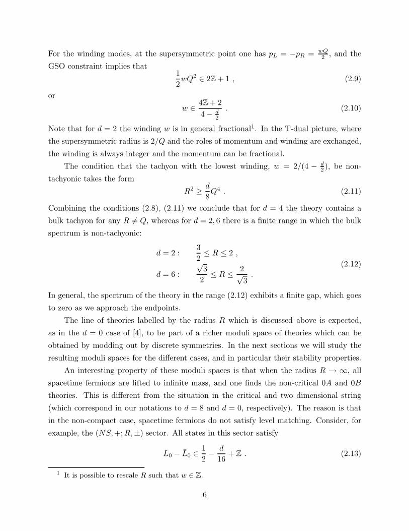
When we compactify, we find the theories depicted in figure 1. Line 1 describes

the compactification of type 0 string theory on a circle. As R → ∞ it approaches the

noncompact 0B theory; as R → 0 one finds the noncompact 0A theory. For any value of

R there are bulk tachyons in the spectrum.

7

Other standard compactifications are the super-affine ones, denoted by lines 2, 3

in figure 1. Since they do not contain spacetime fermions, these compactifications are

simple generalizations of the super-affine compactification of critical type 0 string theory

on IR8,1 × S1. For example the spectrum of line 2 is

(0, 0, 0, 0) , (0, 1, 0, 1) , n ∈ Z , w ∈ 2Z ,

(1, 0, 1, 0) , (1, 1, 1, 1) , n ∈ 1

2+ Z , w ∈ 2Z ,

(1, 0, 1, 1) , (1, 1, 1, 0) , n ∈ Z , w ∈ 2Z + 1 ,

(0, 0, 0, 1) , (0, 1, 0, 0) , n ∈ 1

2+ Z , w ∈ 2Z + 1 .

(3.2)

When R→ ∞ we get 0B and when R→ 0 we get 0A that is equivalent to 0B with R→ ∞.

Again the spectrum contains tachyons for any value of R.

Another way to interpolate between the noncompact 0A and 0B theories is to twist

by (−)α+F . The resulting theory, denoted by line 4 in figure 1, has the spectrum

(0, 0, 0, 0) , (1, 1, 1, 1) , n = m , w = l , m− l ∈ 2Z ,

(1, 0, 0, 0) , (0, 1, 1, 1) , n =1

2+m , w =

1

2+ l , m− l ∈ 2Z ,

(0, 0, 1, 0) , (1, 1, 0, 1) , n =1

2+m , w = −1

2+ l , m− l ∈ 2Z ,

(0, 1, 0, 1) , (1, 0, 1, 0) , n = 1 +m , w = l , m− l ∈ 2Z .

(3.3)

When R→ ∞ we get 0B. When R→ 0 we get 0B, which is equivalent to 0A with R→ ∞.

Thus this line also interpolates between the noncompact 0A and noncompact 0B theories.

SUSY

0A

2 3

1

0B

4

Fig. 1: The moduli space of string theories on IR3,1× IRφ × S1. Line 1 is the

usual compactification that connects type 0A to type 0B. Lines 2 and 3 are the

super-affine compactifications of 0B and 0A. The black boxes represent the self-

dual points along the super-affine lines. The only point at which the theory is

free of bulk tachyons is the supersymmetric one which is on the line of twisted

compactification (line 4).

8

Starting with any line in (3.3) we generate the other lines by acting with (1, 0, 0, 0)(n =12, w = 1

2) and (0, 0, 1, 0)(n = 1

2, w = −1

2). For R = Q =

√2 these operators are holomor-

phic and are identified with the supersymmetry generators (2.2). This is the supersym-

metric point of [1]. As mentioned in section 2, this is the only theory in the moduli space

depicted in figure 1 which is tachyon free.

4. Six dimensional backgrounds I: stability analysis

A particular linear dilaton spacetime of the form (1.1) is the CHS background [5]

IR5,1 × IRφ × SU(2)k , (4.1)

which describes the near-horizon geometry of k NS5-branes. The slope of the linear dilaton

depends on the number of fivebranes via the relation

Q =

√

2

k. (4.2)

This background can also be written in the form (1.3), where the compact manifold is

Mk = SU(2)k/U(1) (the N = 2 minimal model with c = 3− 6k ), and the discrete group is

Γ = Zk. This follows from the decomposition of SU(2)k

SU(2)k =

(

SU(2)k

U(1)× S1

k

)

/Zk . (4.3)

For k = 2, the N = 2 minimal model M2 is empty, and the background (4.1) reduces to

IR5,1 × IRφ × S1 . (4.4)

In the next subsection we study the moduli space corresponding to this case, and then

move on to general k.

4.1. Two fivebranes

In this case, F takes the values, (0, 1) in the NS sector and (−12, 1

2) in the R sector. It

is still defined mod 2, however (−)F belongs to a Z4 rather than a Z2 group. The mutual

locality condition is

F1α2 − F2α1 − F1α2 + F2α1 −1

2(α1α2 − α1α2) + 2(n1w2 + n2w1) ∈ 2Z . (4.5)

9

The two noncompact theories are

0B : (0, 0, 0, 0) , (0, 1, 0, 1) , (1,1

2, 1,

1

2) , (1,−1

2, 1,−1

2) ,

0A : (0, 0, 0, 0) , (0, 1, 0, 1) , (1,1

2, 1,−1

2) , (1,−1

2, 1,

1

2) .

(4.6)

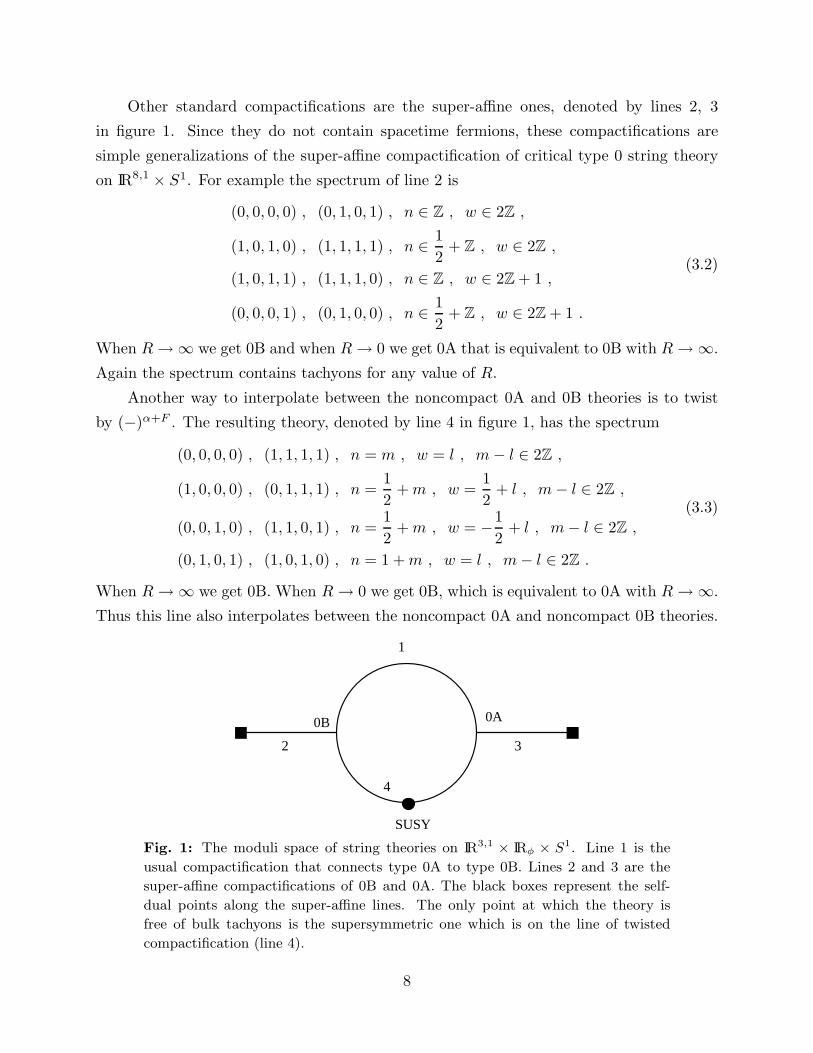
Upon compactification, we find the theories depicted in figure 2. Lines 1, 2 and 3 are as in

the previous section since they do not contain spacetime fermions. Two additional lines of

theories (lines 4, 5) are obtained by starting with the supersymmetric theories of [1] (either

IIB or IIA) and varying R. At the supersymmetric point, the spectrum is determined by

the supercharges, that in the present notation have

G1 = (1,1

2, 0, 0) , n =

1

4, w =

1

2,

G2 = (0, 0, 1,1

2) , n =

1

4, w = −1

2,

(4.7)

in type IIB, and

G1 = (1,1

2, 0, 0) , n =

1

4, w =

1

2,

G2 = (0, 0, 1,−1

2) , n =

1

4, w = −1

2,

(4.8)

in type IIA. One can check that G1 and G2 are mutually local and are holomorphic at

R = Q = 1.

All the states in the theory can be obtained by acting l1 times with G1 and l2 times

with G2 on (0, 0, 0, 0). We denote these states by [l1, l2] = (l1,l12 , l2,± l2

2 ), with a plus

sign in type IIB and a minus sign in type IIA. α and F are defined modulo two, thus

0 ≤ l1, l2 ≤ 3. The momentum and winding modes in each of the sixteen sectors are

determined by the mutual locality of [l1, l2] with respect to G1 and G2. From (4.5) we get

n ∈ Z +1

4(l1 + l2) , w ∈ 2Z +

1

2(l1 − l2) , n+

w

2∈ 2Z +

l12. (4.9)

The tachyon field, for example, is in the [2, 2] = (0, 1, 0, 1) sector. Thus the allowed winding

and momentum modes for the tachyon satisfy

n,w

2∈ Z , n+

w

2∈ 2Z + 1 . (4.10)

The lowest momentum mode has n = 1, while the lowest winding mode has w = 2, in

agreement with the discussion of section 2.

10

Since the spectrum is presented above in terms of n and w (as opposed to pL and pR),

it is simple to generalize the discussion to arbitrary radius. Away from the supersymmetric

pointG1 and G2 are no longer holomorphic; hence, SUSY is broken. As explained in section

2, the theory is tachyon free for3

4≤ R2 ≤ 4

3. (4.11)

The supersymmetric point, R = 1, is in this range. As explained in section 2, it is self-dual;

it is clear from (4.1), that at this point there is an enhanced SU(2)L ×SU(2)R symmetry.

As R→ 0,∞ we find the noncompact 0B, 0A theories.

5

0B 0A

IIBIIA

1

2 3

4

Fig. 2: The moduli space of string theory in IR5,1× IRφ × S1. Lines 1,2 and 3 are

as in figure 1. The black boxes represent the self-dual points along the super-affine

lines. The thick lines are the regions that are free of bulk tachyons.

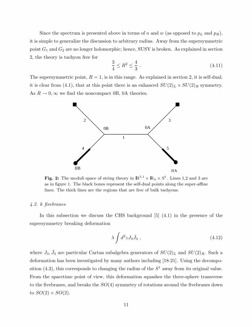
4.2. k fivebranes

In this subsection we discuss the CHS background [5] (4.1) in the presence of the

supersymmetry breaking deformation

λ

∫

d2zJ3J3 , (4.12)

where J3, J3 are particular Cartan subalgebra generators of SU(2)L and SU(2)R. Such a

deformation has been investigated by many authors including [18-21]. Using the decompo-

sition (4.3), this corresponds to changing the radius of the S1 away from its original value.

From the spacetime point of view, this deformation squashes the three-sphere transverse

to the fivebranes, and breaks the SO(4) symmetry of rotations around the fivebranes down

to SO(2) × SO(2).

11

The lightest modes in the background (4.1) are gravitons, whose vertex operators are

given, in the (−1,−1) picture, by2

(

ψψVj

)

j+1;m,m. (4.13)

The dimension of these operators is

∆ =1

2+j(j + 1)

k, (4.14)

where j = 0, 12 , 1, · · · , k

2 − 1. From the point of view of the decomposition (4.3) we can

think of (4.14) as being a sum of two contributions. One comes from the SU(2)U(1) part and

is equal to

∆SU(2)U(1) =

1

2+j(j + 1) −m2

k, m = −j − 1,−j,−j + 1, · · · , j + 1 , (4.15)

with a similar formula for the right-movers. The second contribution to the dimension

comes from the U(1) part and is equal to

∆U(1) =m2

k, (4.16)

again with a similar formula for the right-movers. The U(1) part of the dimension comes

from momentum and winding on a circle. Thus, we have

∆U(1) =1

2p2

L , ∆U(1) =1

2p2

R , (4.17)

with

pL =n

R+wR

2, pR =

n

R− wR

2. (4.18)

Working in conventions where the winding number is an integer, we have

R =Q =

√

2

k,

n =m+ m

k,

w =m− m .

(4.19)

2 To simplify the equations we have omitted the contribution of IR5,1× IRφ to these vertex

operators.

12

Note that while the winding number is an integer, the momentum can be fractional, n ∈Z/k due to the Zk orbifold in (4.3). States that carry non-trivial Zk charge in SU(2)k

U(1)have

fractional momentum n (4.19).

Now we change the radius from the supersymmetric point Rsusy = Q =√

2k to some

other value, R. We would like to find the values of R for which the theory is tachyon free.

As we vary R, the operators (4.13) retain the property that L0 = L0, so it is sufficient to

focus on, say, the left moving part. The dimension of the operator (4.13) for generic R is

given by (omitting the 12

in (4.15)):

j(j + 1) −m2

k+

1

2p2

L . (4.20)

Adding the Liouville contribution, we have

(j + 12 )2 −m2

k+

1

2p2

L − 1

2(β +

Q

2)2 . (4.21)

The delta-function normalizable states in the cigar have β = −Q2 + ip, so the last term in

(4.21) is positive. If the expression (4.21) is positive, the relevant state is massive, while if

it is negative, it is tachyonic.

We see immediately that for all |m| ≤ j, the states in the throat are never tachyonic.

The only way to get tachyons for any radius R is to consider the case |m| = |m| = j + 1,

i.e. m = m = j + 1, or m = −m = j + 1. The two are related by T duality, so it is enough

to analyze the first, which corresponds to pure momentum modes, with pL = pR = 2(j+1)kR .

The condition for this momentum mode to be non-tachyonic is

(j + 12 )2 − (j + 1)2

k+

1

2p2

L > 0 (4.22)

or

R2 <2

k

(j + 1)2

j + 34

. (4.23)

Thus j = 0 is the first state that becomes tachyonic. This happens at R2 = 83k , i.e. 4

3

times the original radius at the supersymmetric point. Repeating the analysis for winding

modes we conclude that the theory is (bulk) tachyon free for

3

2k≤ R2 ≤ 8

3k, (4.24)

in agreement with the result we got for k = 2, (4.11).

13

4.3. Localized instabilities

In the previous subsections we saw that in the six dimensional case, there is a finite

range of radii, for which the bulk theory in the fivebrane throat is non-tachyonic (in fact,

it exhibits a finite mass gap). This is different from the four dimensional case, where the

gap vanishes, and bulk tachyons appear immediately as we change the radius. We note

in passing that in other four dimensional linear dilaton backgrounds, where the manifold

M in (1.3) is non-trivial, the gap is finite as well, and the situation is similar to the six

dimensional examples.

In theories with a finite gap in the bulk spectrum, there are no bulk instabilities even

when we break supersymmetry (sufficiently mildly). A natural question, which we will

address in this subsection, is whether such theories have localized instabilities.

In the six dimensional system (4.1) we understand the low energy dynamics in terms

of the theory on NS5-branes. Consider, for example, the type IIB case.3 At the supersym-

metric point, the low energy theory on the fivebranes is a six dimensional super Yang-Mills

theory with sixteen supercharges, and gauge group SU(k) (for k fivebranes). This theory

has a moduli space parameterized by the locations of the fivebranes in the transverse IR4.

Denoting the positions of the fivebranes in the four transverse directions by the k × k

matrices

A = x6 + ix7 , B = x8 + ix9 , (4.25)

one can parameterize points in the moduli space of separated fivebranes by the expectation

values of gauge invariant operators such as TrAn, TrBn, etc.

In the supersymmetric theory, it is well understood [7,22,23] how to describe separated

fivebranes in the geometry (4.1). For example, if the fivebrane configuration has a non-zero

expectation value of TrB2j+2, the worldsheet theory should be deformed by the operator

e−ϕ−ϕψ+ψ+Vj;j,je−Q(j+1)φ . (4.26)

This operator corresponds to a wavefunction that is supported in the strong coupling region

of the linear dilaton space IRφ. It is an example of a localized state in the throat. This is

in agreement with the spacetime picture, according to which it describes a scalar living on

the fivebranes.

3 A similar discussion holds for IIA fivebranes.

14

A particularly symmetric deformation of the kind (4.26) that has been extensively

studied corresponds to placing the fivebranes on a circle of size r0 in the B plane

Bl = r0e2πil

k , Al = 0 , l = 1, 2, ..., k . (4.27)

In the bulk, this is described by condensation of the mode (4.26) with j = k2 − 1. It is

useful to write this operator in the decomposition (4.3). By looking at equation (4.15),

and using the fact that it has m = j + 1 = k2, we see that from the point of view of SU(2)

U(1)

it is proportional to the identity operator. In fact, it is the N = 2 Liouville superpotential

W = ei 1R

x− 1Q

φ , (4.28)

where R = Q is the radius at the supersymmetric point (4.19). As is well known, the

N = 2 Liouville operator is truly marginal, and signals the change from IRφ × S1 to the

cigar (here we are describing it in terms of the T-dual variables, so the N=2 Liouville

perturbation is a momentum mode). Note that we are not assuming here that the string

coupling is weak everywhere. It could be that the string coupling at the tip of the cigar is

very large, but we are studying the weakly coupled region where it is small.

Now suppose we change the radius R from its original value (4.19). There are two

different cases to discuss. If we make R smaller, the operator (4.28), which had dimension

one before, will have dimension larger than one. This means that it is massive, and we

have to dress (4.28) with a time-dependent part, like cos(Et) with a real energy E. This

means that 〈TrBk〉, and the size of the circle on which the fivebranes are placed, r0 (4.27),

will oscillate between two extreme values.

On the other hand, if we increase the radius R, the dimension of (4.28) drops below

one, it becomes tachyonic, and to make it physical we have to dress it with, e.g., cosh(Et)

with a real E. This means that r0 increases without bound (in this approximation) as

|t| → ∞. In the next section we explore in details these dynamical processes using various

techniques.

5. Six dimensional backgrounds II: Time dependence, field theory and gravity

In this section we further discuss the deformed NS5-brane background with broken

supersymmetry obtained by applying the perturbation (4.12). In the first subsection we

construct time-dependent solutions that correspond to rolling fivebranes. In the second

subsection we comment on the description of the deformed fivebrane system using the low

energy field theory and supergravity. The latter is valid at large k.

15

5.1. Rolling fivebranes

At the end of the last section we briefly mentioned the time-dependent solutions

obtained by displacing the fivebranes from the origin of the moduli space A = B = 0 (4.25)

in the presence of the supersymmetry breaking deformation (4.12). We only discussed what

happens to leading order in the separation of the fivebranes (4.28), since we only imposed

the leading order condition that the dressed perturbation be marginal. In general, one

expects the solution to receive corrections, and for the solutions mentioned in the previous

section we expect these to be large. The reason is that these solutions correspond to

accelerating fivebranes, and are expected to radiate. Since the tension of the NS5-branes

scales like 1/g2s , the closed strings radiation (that goes like GNT5) is an order one effect

that influences the solution in a non-trivial way at tree level.4

Nevertheless, it is possible to find exact solutions of the classical string equations of

motion that correspond to rolling fivebranes. Consider first the case of decreasing the

radius R, such that the N = 2 Liouville operator (4.28) becomes irrelevant (or massive).

In that case, we can make it marginal by replacing (4.28) with

W = eiR

x+iωRt− 1Q

φ . (5.1)

The mass-shell condition requires that

ω2R =

1

R2− 1

Q2. (5.2)

We can define a coordinate xnew by

1

Qxnew =

1

Rx+ ωRt . (5.3)

The condition (5.2) implies that xnew is canonically normalized (when x and t are). In

terms of this new field, the perturbation separating the fivebranes (5.1) looks precisely like

the N = 2 Liouville perturbation again. Thus, we conclude that (5.1) is a truly marginal

deformation. It describes the fivebranes placed on the slope of the quadratic potential and

rotating around the circle with angular velocity ωR (see figure 3a). The existence of an

exact CFT description implies that there should also be a supergravity solution associated

with that system. This solution is described in the appendix.

4 This is different from the well studied case of unstable D-branes with a rolling tachyon [24].

There, the closed strings radiation is an order gs effect [25,26], and so can be neglected (at least

formally) in the leading approximation.

16

(a) (b)

Fig. 3: Time dependent processes which have exact CFT descriptions: (a) Five-

branes rotating around a circle with a constant angular velocity; (b) Fivebranes

moving radially with a constant radial velocity.

The orthogonal combination of (t, x) is timelike,

1

Qtnew =

1

Rt+ ωRx . (5.4)

The original periodicity of x, x ∼ x+ 2πR translates in terms of the new coordinates to:

(tnew, xnew) ∼ (tnew, xnew) + 2πQ(ωRR, 1) . (5.5)

One can describe the solution of fivebranes rotating around the circle by a coset CFT. The

supersymmetric solution corresponding to fivebranes on a circle can be thought of as

IR5,1 × SL(2, IR)k × SU(2)k (5.6)

modded out by the null U(1) symmetry generated by the current

J = J3 −K3 , (5.7)

where J3 and K3 are the Cartan subalgebra generators of SL(2) and SU(2) respectively.

In order to go from this solution to the one described by (5.1), we need to mix the U(1)

current K3 with the timelike U(1), i∂t. Ignoring the periodicity conditions, this is simply

17

a boost transformation. Thus, in terms of the coset description (5.6), (5.7), we want to

gauge the current

J3 − β1K3 −iβ2

Q∂t , (5.8)

where the boost parameters βi satisfy β21−β2

2 = 1. This provides an exact CFT description

of the system of fivebranes rotating around the circle.

Naively, one might expect that as the fivebranes are rotating around the circle they

should radiate, and the solution should be modified, already at tree level. This seems in

contradiction to the fact that we found an exact solution of the full equations of motion of

classical closed string theory. The resolution of this puzzle is that in the near-horizon limit,

the solution with fivebranes rotating around the circle corresponds to motion with constant

velocity, and not constant acceleration (since the near-horizon metric for the angular S3

is dΩ2 and not r2dΩ2). Thus, it does not radiate.

This should be contrasted with the case where we place the fivebranes at some distance

from the origin and let them go. In this case, one expects the system to oscillate about the

minimum, with r0 ∼ cosωRt. This amounts to replacing exp(iωRt) in (5.1) with cos(ωRt).

From the spacetime point of view, we expect non-zero radiation in this case, since this

solution corresponds to a time dependence of φ of the form φ ∼ log cosωRt. Thus, there

is in this case non-zero acceleration, and we expect the solution to be modified at the

tree level. This is natural from the worldsheet point of view. If we replace exp(iωRt)

by cos(ωRt) in (5.1), the operator (5.1) ceases to be holomorphic, and one expects it

to become marginally relevant (like the marginal Sine-Gordon and non-Abelian Thirring

model couplings). Presumably, this behavior of the worldsheet theory is directly related

to the classical radiation that one expects in spacetime.

For the other case, of increasing5 radius R, for which wR is imaginary, the operator

(4.28) is relevant, and we expect to have to dress it with a real exponential in time. Thus,

instead of (5.1) we now have

W = eiR

x+wRt− 1Q

φ , (5.9)

and wR is given by (similarly to (5.2))

w2R =

1

Q2− 1

R2. (5.10)

5 T-duality relates increasing R to decreasing R, while exchanging momentum and winding

modes. Therefore, instead of increasing R we can continue to decrease it and study other classical

solutions.

18

We would like again to make an N = 2 Liouville perturbation out of (5.9), so we define a

new Liouville coordinate φnew by

1

Rφnew =

1

Qφ− wRt . (5.11)

Again, due to (5.10), φnew is canonically normalized. Now, in terms of φnew and x we

again have an N = 2 Liouville theory, so this is an exact solution of the equations of

motion of the theory, corresponding to fivebranes approaching the origin of the B plane

as t → −∞, and moving out to infinity at t → +∞ (see figure 3b). This is an analog

of the “half-brane” from unstable D-brane dynamics. Note that, as in the discussion of

fivebranes rotating around a circle, during the time evolution no radiation is emitted, since

the fivebranes are moving with constant velocity in the φ direction. The relevant “rolling

fivebrane” supergravity solution is constructed in the appendix.

One thing that is different in this case relative to the previous one is that since we

are mixing the time coordinate with φ to make the cigar, the remaining combination of φ

and t,1

Rtnew =

1

Qt− ωRφ (5.12)

which does not participate in the cigar and is timelike, has a linear dilaton associated with

it. More precisely, one finds,

Qφnew= R , Qtnew

= QRωR . (5.13)

This signals the fact that at early times (t, tnew → −∞), when the fivebranes are on top of

each other, we have a strong coupling problem, despite the fact that we have constructed

a cigar which avoids the strong coupling problem in the direction φnew.

Again, one can describe the time-dependent background (5.9) by an exact coset CFT.

As we see from (5.11), (5.12), in this case we need to perform a boost mixing φ and t, or

J3 and ∂t. One can describe this background as (5.6) modded out by the null current

J3 +β1

Q∂t− β2K3 , (5.14)

with β21 + β2

2 = 1.

The solution describing fivebranes running to infinity as a function of time is an

example of localized tachyon condensation. In our case we are able to find an exact CFT

that describes this time-dependent process, and smoothing out of the singularity, while in

19

the case of non-supersymmetric orbifolds [27] no exact time-dependent solutions of this

sort were found. The reason for the difference is that we took the near-horizon limit of

a throat, in which, as we have seen, the smoothing out of the singularity proceeds via a

process in which no radiation is emitted, whereas the analysis of [27], takes place in the

full geometry where one expects the solution to be much more complicated and to involve

non-trivial radiation effects.6

A related point is that here we wrote an exact solution which is an analog of a half

S-brane [29,24] for decaying D-branes. There should exist a more complicated solution

where the distance between the fivebranes starts at t → −∞ very large, decreases to a

minimal value, and then increases back to infinity. This solution would be an analog of

the full S-brane. In this case the φ coordinate accelerates near the turning point, and one

expects non-trivial radiation effects at tree level.

5.2. Dual field theory and supergravity

In this subsection we consider the deformation (4.12) from the point of view of the

dual field theory and supergravity descriptions. We focus on the type IIB case. In this case

the dual field theory is a six dimensional SYM theory with sixteen superchrages and an

SU(k) gauge group. This field theory is infrared free and is believed to resolve the strong

coupling singularity associated with the CHS background [6]. Since the wave function of

(4.26) is concentrated in the strong coupling region, one can study the relevant dynamics

using the dual field theory description.

The relationship between the bulk modes in the CHS background and chiral field

theory operators was described in [7]. The vertex operators (4.13) correspond to symmetric,

traceless combinations of the four scalars (4.25). In particular, the deformation (4.12) is

dual to a mass term for the scalars

αTr(A∗A − B∗B) . (5.15)

Thus, with the deformation two of the four flat directions become massive, while the

other two become tachyonic. This fits nicely with the results of the previous subsection.

The relation between α and R is the following. Normalizing the field B such that the

Lagrangian takes the form

L = |B|2 + α|B|2 , (5.16)

6 The relation between localized tachyons on non-supersymmetric orbifolds and throat theories

was discussed in [28].

20

and comparing the solution of the equation of motion B = r0e±i

√αt to (5.1), we find that

α =1

Q2− 1

R2. (5.17)

Another way to study the dynamics is to use the supergravity description, which

is accurate for large k. First we have to find the deformation of the CHS background

associated with (4.12). In the appendix we describe the relevant solution from the coset

point of view. Here we describe this solution directly in the CHS language.

The starting point is the CHS background associated with k NS5-branes [5],

ds2 = dx2|| + dφ2 + 2k

(

dθ2 + sin2 θdφ21 + cos2 θdφ2

2

)

,

B = k(1 + cos(2θ))dφ1 ∧ dφ2 , g2s = exp(−

√

2/kφ) ,(5.18)

where 0 ≤ θ ≤ π/2, 0 ≤ φ1, φ2 ≤ 2π. The transverse coordinates (4.25) are given by

A =√

2k exp(φ√

1/2k) sin(θ)exp(iφ1) , B =√

2k exp(φ√

1/2k) cos(θ)exp(iφ2) . (5.19)

This relation can be derived by comparing the field theory and the supergravity expressions

for the energy of a BPS D1-brane (or of a fundamental string in the near-horizon geometry

of k D5-branes).

To find the solution associated with the perturbation (4.12) we recall that this defor-

mation can be viewed [30,18,31] as an SL(2, IR) transformation of the usual CHS back-

ground. The relevant SL(2, IR) transformation is

τ → τ′

=τ

1 + ατ, (5.20)

where τ is the Kahler parameter, τ ≡ B12 + i√g = 2k cos(θ)eiθ. A short calculation yields

ds2 = dx2|| + dφ2 + 2k

(

dθ2 +1

(1 + kα)2 + tan2 θ(tan2 θdφ2

1 + dφ22)

)

,

B =2k(1 + kα)

(1 + kα)2 + tan2 θdφ1 ∧ dφ2 , g2

s = e−φ√

2/k 1 + tan2 θ

(1 + kα)2 + tan2 θ.

(5.21)

This solution is not quite what we are after since it has a conical singularity at θ = 0. This

can be fixed by rescaling φ1 → φ1/(1 + kα), which yields

ds2 = dx2|| + dφ2 + 2k

(

dθ2 +1

L2 + tan2 θ(L2 tan2 θdφ2

1 + dφ22)

)

,

B =2kL2

L2 + tan2 θdφ1 ∧ dφ2 , g2

s = e−φ√

2/k 1 + tan2 θ

L2 + tan2 θ,

(5.22)

21

where L = 1 + αk. The curvature in string units is small as long as k ≫ 1 and L− 1 ≪ 1.

We wish to show that this background indeed exhibits the same physics as (5.15).

Namely, it has two massive directions and two tachyonic ones. To this end we calculate

the potential felt by a probe fivebrane that is localized in φ and on the sphere. This

potential is the strong coupling dual of (5.15). In general such a calculation need not yield

the same result. However, since for |α| ≪ 1 we are in the near BPS limit we expect to find

the same potential to leading order in α.

To see that this is indeed the case, consider the DBI action of a probe D5-brane

propagating in the S-dual background,

ds2 = gs

[

dx2|| + dφ2 + 2k

(

dθ2 +1

L2 + tan2 θ(L2 tan2 θdφ2

1 + dφ22)

)]

,

F3 =−4kL2 tan(θ)(1 + tan2 θ)

(L2 + tan2 θ)2dφ1 ∧ dφ2 ∧ dθ , g2

s = eφ√

2/kL2 + tan2 θ

1 + tan2 θ.

(5.23)

The six-form potential that couples to the D5-brane probe is A|| = Leφ√

2/k and the DBI

potential reads

V = g−1s

√g|| −A|| = eφ

√2/k

(

L2 + tan2 θ

1 + tan2 θ− L

)

. (5.24)

Using (5.19) we can express this potential in terms of the field theory variables. For small

deformation, α≪ 1, we find,

V = α (A∗A−B∗B) , (5.25)

in agreement with (5.15) .

6. Two dimensional background

In this section we study superstrings on IR1,1 × IRφ × S1, with Q =√

3. The analysis

here is fairly similar to the one in section 4.1. Like in the six dimensional case, F takes the

values (0, 1) in the NS sector and (−12 ,

12 ) in the R sector. The mutual locality condition

is slightly different than in the six dimensional case

F1α2 − F2α1 − F1α2 + F2α1 +1

2(α1α2 − α1α2) + 2(n1w2 + n2w1) ∈ 2Z . (6.1)

The moduli space is very similar to that of figure 2. The type 0 and super-affine lines 1, 2, 3

are as there. As in the six dimensional case, there are two additional lines of theories that

are obtained by starting with the supersymmetric theories (either IIA or IIB) and varying

22

R. These theories can be analyzed using the same approach as in section 4.1. Now the

supersymmetry generators are

G1 = (1,1

2, 0, 0) , n =

3

4, w =

1

2,

G2 = (0, 0, 1,1

2) , n =

3

4, w = −1

2,

(6.2)

in type IIB, and

G1 = (1,1

2, 0, 0) , n =

3

4, w =

1

2,

G2 = (0, 0, 1,−1

2) , n =

3

4, w = −1

2,

(6.3)

in type IIA. With the help of (6.1) we find that the winding and momentum modes in the

[l1, l2] sector satisfy

n ∈ Z − 1

4(l1 + l2) , 3w ∈ 2Z +

1

2(l2 − l1) , n+

3

2w ∈ 2Z − 1

2l1 . (6.4)

For the tachyon modes (in the [2, 2] sector), we find, in agreement with section 2, that

the lowest momentum is one, and the lowest winding is 23 . As explained in section 2 this

implies that the theory is free of bulk tachyons for 32 ≤ R ≤ 2. The supersymmetric radius,

R =√

3, is self-dual under T-duality. However, here, unlike the six dimensional case, the

symmetry is not enhanced to SU(2)L×SU(2)R at this point. Again, these lines interpolate

between 0B (0A) and 0B (0A).

While the physics in the bulk of the linear dilaton throat is quite similar to the six

dimensional case, the localized dynamics is different. In the six dimensional case, there

was an instability due to localized tachyons such as the N = 2 Liouville mode (4.28), which

was massless for R = Q and became tachyonic when R 6= Q. This deformation exists also

in the two dimensional case. However since now Q >√

2, this mode is non-normalizable

(for recent discussions, see [10,11] ), and hence it cannot dynamically condense. In fact, in

this case there are no normalizable localized tachyons, so the non-supersymmetric model

is locally stable.

7. Three dimensional backgrounds

The theories we considered in the previous sections have the property that the N = 2

Liouville operator (4.28) is in the spectrum. Since this mode is tachyonic for R 6= Q,

Q <√

2, one might be tempted to conclude that there are no stable non-supersymmetric

23

deformations of linear dilaton backgrounds with a small dilaton slope. This conclusion is

incorrect.

A counter example is the background

IR2,1 × IRφ × SU(2)k1× SU(2)k2

, (7.1)

with

Q =

√

2

k,

1

k=

1

k1+

1

k2. (7.2)

We will see that a small non-supersymmetric deformation of the form (4.12), acting on

either of the two SU(2)’s in (7.1), does not lead to instabilities in this case.

The background (7.1) is the near-horizon geometry of the intersection of k1 coincident

NS5-branes stretched in the directions (012345) and k2 coincident NS5-branes stretched in

(016789) (see [13] for a recent discussion). This brane configuration is Poincare invariant in

1+1 dimensions, but the near-horizon geometry (7.1) exhibits a higher Poincare symmetry,

in 2 + 1 dimensions [13].

In section 4 we considered the system of k parallel NS5-branes and argued in three

different ways for instability when (4.12) is turned on. For the background (7.1) all these

arguments indicate that the system is stable.

(1) From the worldsheet point of view the instability was due to the fact that the N = 2

Liouville mode became tachyonic when we changed the radius. Now, however, this

mode is not in the spectrum [13]. This is possible because this theory is not of the

form (1.3).

(2) The dual field theory argument for the instability was that some of the flat directions

at R = Rsusy became tachyonic when R 6= Rsusy. The field theory dual to (7.1),

however, has a mass gap [13,14]. Hence a small deformation of the parameters cannot

lead to a tachyonic mode. The flat directions in the case of k parallel NS5-branes

were associated with moving the branes in the transverse directions. In our case

these deformations are massive, since each stack of fivebranes is wrapped around a

three-sphere (see [13] for a more extensive discussion).

(3) A complementary argument for instability came from the probe fivebrane dynamics

(see section 5.2). Is it possible that a probe fivebrane in the background (7.1) that

respects three dimensional Poincare invariance has a flat direction and can become

unstable away from the supersymmetric point? To verify that this is not the case let us

calculate the potential experienced by such a probe fivebrane. Again it is convenient

24

to work with S-dual variables and study the DBI action for a probe D5-brane. The

S-dual metric and dilaton take the form

ds2 = gs

[

−dx20 + dx2

1 + dx22 + dφ2 + 2k1dΩ

23 + 2k2dΩ

23

]

, g2s = eφQ , (7.3)

and the RR-fields are

F3 = 2k1 sin(2θ)dφ1 ∧ dφ2 ∧ dθ + 2k2 sin(2θ)dφ1 ∧ dφ2 ∧ dθ . (7.4)

To compute the DBI action of a probe D5-brane we need the dual field strength

F7 = ⋆F3 = 2eQφ[

k1 sin(2θ)(k2/k1)3/2dx|| ∧ dφ ∧ dΩ+

+k2 sin(2θ)(k1/k2)3/2dx|| ∧ dφ ∧ dΩ

]

,(7.5)

from which we find the six-form that couples to the D5-brane

A6 = 2eQφ

[

k1

Q(k2/k1)

3/2 sin(2θ)dx|| ∧ dΩ +k2

Q(k1/k2)

3/2 sin(2θ)dx|| ∧ dΩ]

. (7.6)

Thus the potential felt by a probe D5-brane stretched along (x0, x1, x2, S3) and local-

ized at some φ, is attractive

∫

S2

g−1s

√g||gS2 −A6 = 4π2V||e

Qφ√

2k3/22

(

1 −√

k2

k1 + k2

)

. (7.7)

The analog of (5.19) for this case implies that the scalar fields are proportional to

exp(Qφ/2). Thus (7.7) takes the form of a mass term for the scalars. This is in

agreement with the field theory analysis of [13] that leads to a mass gap in the dual

field theory.

Acknowledgements

We thank J. Maldacena for a discussion. DK thanks the Weizmann Institute, Rutgers

NHETC and Aspen Center for Physics for hospitality during parts of this work. NI thanks

the Enrico Fermi Institute at the University of Chicago for hospitality. The work of DK

is supported in part by DOE grant DE-FG02-90ER40560; that of NS by DOE grant DE-

FG02-90ER40542. NI is partially supported by the National Science Foundation under

Grant No. PHY 9802484. Any opinions, findings, and conclusions or recommendations

expressed in this material are those of the authors and do not necessarily reflect the views

of the National Science Foundation.

25

Appendix A. Time dependent supergravity solutions

In section 5 we argued that there are exact CFT’s, (5.1) and (5.9), that describe

certain time dependent NS5-brane configurations. The aim of this appendix is to construct

the supergravity solutions associated with these CFT’s. Both (5.1) and (5.9) are exactly

marginal deformations of the coset(

S1k × SU(2)k

U(1)

)

/Zk. When thinking about the relevant

supergravity solutions it is more natural to use the SU(2)k description. Therefore, we first

review the details of the transformation that takes the SU(2)k to(

S1k × SU(2)k

U(1)

)

/Zk. We

start on the SU(2)k side (in this appendix we set α′ = 1)

ds2 = k(

dθ2 + sin2 θdφ21 + cos2 θdφ2

2

)

, B12 = k cos2 θ , (A.1)

where 0 ≤ θ ≤ π/2, 0 ≤ φ1, φ2 ≤ 2π. The complex and Kahler structures associated with

this background are

τ =g12g22

+ i

√g

g22= i tan θ , τk = B12 + i

√g = k cos θeiθ . (A.2)

To transform to the(

S1k × SU(2)k

U(1)

)

/Zk description we first apply T-duality in the φ2

direction. This amounts to τ ↔ τk (for a review see [32]) so we find the T-dual background

to be

ds2 = k(dθ2 + dφ21) + 2dφ1dφ2 +

1

k cos2 θdφ2

2 , B12 = 0 . (A.3)

Defining new coordinates

φ1 = φ1 + φ2/k , φ2 = φ2/k , (A.4)

we find

ds2 = k(

dθ2 + dφ21 + tan2 θdφ2

2

)

. (A.5)

Note that now we have a Zk identification, (φ1, φ2) ∼ (φ1 +2π/k, φ2 +2π/k), that implies

that the background is indeed(

S1k × SU(2)k

U(1)

)

/Zk. As usual the dilaton picks an extra

factor from the T-duality transformation gs → gs(detgnew/detgold)1/4, so we have

gs → gs

cos θ. (A.6)

Now we shall deform the(

S1k × SU(2)k

U(1)

)

/Zk side in various ways and see what these

deformations give on the SU(2)k side.

26

(1) The supersymmetry breaking deformation (4.12) corresponds to changing the radius

of the S1 from√k to L

√k. The resulting metric on the squashed sphere is

ds2 = k(

dθ2 + L2dφ21 + tan2 θdφ2

2

)

, gs =1

cos θ. (A.7)

The change of coordinates (A.4) leads to

ds2 = k

(

dθ2 + L2dφ21 +

2L2

kdφ1dφ2 +

L2 + tan2 θ

k2dφ2

2

)

. (A.8)

Applying T-duality in the φ2 direction we get

ds2 = k

(

dθ2 +L2 tan2 θ

L2 + tan2 θdφ2

1 +1

L2 + tan2 θdφ2

2

)

B12 =kL2

L2 + tan2 θ, g2

s =1 + tan2 θ

L2 + tan2 θ.

(A.9)

This agrees with the SU(2) contribution to (5.22).

(2) Another useful background is obtained by adding a direction, ρ, and combining it

with φ1 to form a cigar(

SL(2)k

U(1) × SU(2)k

U(1)

)

/Zk. This does not change the asymptotic

radius of the S1, so at large ρ the background is SU(2)k × IR. The metric is

ds2 = k(

dθ2 + tan2 θdφ22 + dρ2 + tanh2 ρdφ2

1

)

, gs =1

cos θcoshρ, (A.10)

where (φ1, φ2) ∼ (φ1 + 2π/k, φ2 + 2π/k). Now we wish to find the effect of this

deformation in the SU(2) variables. Using (A.4) we get

ds2 = k(

dθ2 + dρ2 + tanh2 ρdφ21

)

+2 tanh2 ρdφ1dφ2+1

k(tan2 θ+tanh2 ρ)dφ2

2 . (A.11)

Applying T-duality we get

ds2 = k

(

dθ2 + dρ2 +tan2 θ tanh2 ρ

tan2 θ + tanh2 ρdφ2

1 +1

tan2 θ + tanh2 ρdφ2

2,

)

B =k tanh2 ρ

tan2 θ + tanh2 ρ, g2

s =1

cos2 θ cosh2ρ(tan2 θ + tanh2 ρ).

(A.12)

When ρ → ∞ we get back the CHS solution. The full solution corresponds to a ring

of fivebranes in the B plane. A simple way to see this is to note that the dilaton

diverges at θ = ρ = 0, which is indeed a point in the B plane (see eq. (5.19)).

27

(3) Combining the backgrounds (1) and (2) leads to(

SL(2)L2k

U(1) × SU(2)k

U(1)

)

/Zk. The asymp-

totic radius is L√k and we also have a cigar. This is the supergravity description of

the deformed fivebranes theory perturbed by (5.9). The spacetime fields take the form

ds2 = k(

L2(dρ2 + tanh2 ρdφ21) + dθ2 + tan2 θdφ2

2

)

, gs =1

cos θ coshρ, (A.13)

with the usual Zk identifications (φ1, φ2) ∼ (φ1 + 2π/k, φ2 + 2π/k). Following the

steps above, we first use (A.4) to find

ds2 = kdθ2+L2kdρ2+L2k tanh2 ρdφ21+

1

k(L2 tanh2 ρ+tan2 θ)dφ2

2+2L2 tanh2 ρdφ1dφ2.

(A.14)

Applying T-duality we get

ds2 = k

(

dθ2 + L2dρ2 +L2 tan2 θ tanh2 ρ

L2 tanh2 ρ+ tan2 θdφ2

1 +1

L2 tanh2 ρ+ tan2 θdφ2

2

)

,

B =L2 tanh2 ρ

L2 tanh2 ρ+ tan2 θ, g2

s =1

cos2 θcosh2ρ(L2 tanh2 ρ+ tan2 θ).

(A.15)

Now we can write down the supergravity solution that corresponds to the deformation

(5.9)

ds2 = −dt2new + dφ2new + dx2

||+

k

(

dθ2 +L2 tan2 θ tanh2(φnew/L

√k)

L2 tanh2(φnew/L√k) + tan2 θ

dφ21 +

1

L2 tanh2(φnew/L√k) + tan2 θ

dφ22

)

,

B =L2k tanh2(φnew/L

√k)

L2 tanh2(φnew/L√k) + tan2 θ

,

g2s =

1

cos2 θcosh2(φnew/L√k)(L2 tanh2(φnew/L

√k) + tan2 θ)exp(2αtnew)

,

(A.16)

where

α2 =1

k(

1

L2− 1) (A.17)

and L < 1. A simple way to find the relation between tnew, φnew and the original

coordinates t, φ is to note that asymptotically the background is not deformed. This

gives

φ =1

Lφnew +

√kαtnew , t =

1

Ltnew +

√kαφnew , (A.18)

in agreement with (5.11).

28

To verify that this solution indeed describes a ring of NS5-branes which run away to

infinity we note that the dilaton diverges when θ = φnew = 0. In terms of the original

coordinates, the trajectory of the fivebranes is

φ =

(

1

L− L

)

t . (A.19)

(4) Now we wish to find the supergravity solution that corresponds to (5.1). For this we

have to proceed in a slightly different way. At large ρ the metric takes the form

ds2 = kdρ2 + dx2 − dt2 + ... (A.20)

where x ∼ x+2πR and R = L√k with L < 1. Clearly we can define a new coordinates

system obtained by a boost

xnew = Cx+ St , tnew = Ct+ Sx , C2 − S2 = 1 (A.21)

so that the metric at infinity takes the form

ds2 = kdρ2 + dx2new − dt2new + · · · . (A.22)

Now we can deform (A.22) to obtain a cigar like geometry

ds2 = kdρ2 + tanh2 ρ dx2new − dt2new + ... (A.23)

Since x is periodic this cannot be done for any boost parameter, C. To avoid a conical

singularity we must impose

C2 =k

R2=

1

L2. (A.24)

This condition is equivalent by T-duality to (5.3). Writing (A.23) using t and φ1 =

x/R we get

ds2 =dx2|| + k(dρ2 + dθ2 + tan2 θdφ2

2) + dφ21(k tanh2 ρ− S2R2)

− dt2(C2 − tanh2 ρS2) + 2dφ1dtCSR(tanh2 ρ− 1) .(A.25)

Now we can follow the same steps as above. First we change coordinate from φi to

φi. This gives (with the help of (A.24))

ds2 =dx2|| + k(dρ2 + dθ2) + k(tanh2 ρ− ǫ)dφ2

1 −1

L2(1 − ǫ tanh2 ρ)dt2+

1

k(tanh2 ρ+ tan2 θ − ǫ)dφ2

2 + 2(tanh2 ρ− ǫ)dφ1dφ2

− 2

√ǫk

L

1

cosh2ρdtdφ1 −

2

L

√

ǫ

k

1

cosh2ρdtdφ2 ,

(A.26)

29

where ǫ = 1 − L2. Applying T-duality in the φ2 direction we get

g22 =1

g22=

k

tanh2 ρ+ tan2 θ − ǫ,

g11 =1

g22(g11g22 − g2

12) =k tan2 θ(tanh2 ρ− ǫ)

tanh2 ρ+ tan2 θ − ǫ,

gtt =1

g22(gttg22 − g2

t2) = −tan2 θ + tanh2 ρ(L4 − ǫ tan2 θ)

L2(tanh2 ρ+ tan2 θ − ǫ),

gt1 =1

g22(gt1g22 − gt2g12) =

√

ǫk

L2

tan2 θ

cosh2ρ(tanh2 ρ+ tan2 θ − ǫ),

Bt2 =gt2

g22= −

√

ǫk

L2

1

cosh2ρ(tanh2 ρ+ tan2 θ − ǫ),

B12 =g12g22

= kBt2 .

(A.27)

This solution describes rotation in the A plane (as opposed to the previous case where

the branes move in the B plane) since gt2 vanishes and gt1 does not.

30

References

[1] D. Kutasov and N. Seiberg, “Noncritical Superstrings,” Phys. Lett. B 251, 67 (1990).

[2] T. Banks and L. J. Dixon, “Constraints On String Vacua With Space-Time Super-

symmetry,” Nucl. Phys. B 307, 93 (1988).

[3] M. Dine and N. Seiberg, “Microscopic Knowledge From Macroscopic Physics In String

Theory,” Nucl. Phys. B 301, 357 (1988).

[4] N. Seiberg, “Observations on the moduli space of two dimensional string theory,”

JHEP 0503, 010 (2005) [arXiv:hep-th/0502156].

[5] C. G. Callan, J. A. Harvey and A. Strominger, “Supersymmetric string solitons,”

arXiv:hep-th/9112030.

[6] N. Itzhaki, J. M. Maldacena, J. Sonnenschein and S. Yankielowicz, “Supergravity and

the large N limit of theories with sixteen supercharges,” Phys. Rev. D 58, 046004

(1998) [arXiv:hep-th/9802042].

[7] O. Aharony, M. Berkooz, D. Kutasov and N. Seiberg, “Linear dilatons, NS5-branes

and holography,” JHEP 9810, 004 (1998) [arXiv:hep-th/9808149].

[8] A. Giveon, D. Kutasov and O. Pelc, “Holography for non-critical superstrings,” JHEP

9910, 035 (1999) [arXiv:hep-th/9907178].

[9] S. Murthy, “Notes on non-critical superstrings in various dimensions,” JHEP 0311,

056 (2003) [arXiv:hep-th/0305197].

[10] J. L. Karczmarek, J. Maldacena and A. Strominger, “Black hole non-formation in the

matrix model,” arXiv:hep-th/0411174.

[11] A. Giveon, D. Kutasov, E. Rabinovici and A. Sever, “Phases of quantum gravity in

AdS(3) and linear dilaton backgrounds,” Nucl. Phys. B 719, 3 (2005) [arXiv:hep-

th/0503121].

[12] D. Kutasov and N. Seiberg, “Number Of Degrees Of Freedom, Density Of States And

Tachyons In String Theory And Cft,” Nucl. Phys. B 358, 600 (1991).

[13] N. Itzhaki, N. Seiberg and D. Kutasov, “I-brane dynamics,” arXiv:hep-th/0508025.

[14] H. Lin and J. Maldacena, “Fivebranes from gauge theory,” arXiv:hep-th/0509235.

[15] O. Bergman and S. Hirano, “Semi-localized instability of the Kaluza-Klein linear dila-

ton vacuum,” arXiv:hep-th/0510076.

[16] M. Dine, P. Y. Huet and N. Seiberg, “Large And Small Radius In String Theory,”

Nucl. Phys. B 322, 301 (1989).

[17] J. Polchinski, “String theory. Vol. 2: Superstring theory and beyond” Cambridge press.

[18] S. F. Hassan and A. Sen, “Marginal deformations of WZNW and coset models from

O(d,d) transformation,” Nucl. Phys. B 405, 143 (1993) [arXiv:hep-th/9210121].

[19] E. Kiritsis and C. Kounnas, “Infrared behavior of closed superstrings in strong mag-

netic and Nucl. Phys. B 456, 699 (1995) [arXiv:hep-th/9508078].

31

[20] T. Suyama, “Deformation of CHS model,” Nucl. Phys. B 641, 341 (2002) [arXiv:hep-

th/0206171].

[21] S. Forste and D. Roggenkamp, “Current current deformations of conformal field the-

ories, and WZW JHEP 0305, 071 (2003) [arXiv:hep-th/0304234].

[22] A. Giveon and D. Kutasov, “Little string theory in a double scaling limit,” JHEP

9910, 034 (1999) [arXiv:hep-th/9909110].

[23] A. Giveon and D. Kutasov, “Comments on double scaled little string theory,” JHEP

0001, 023 (2000) [arXiv:hep-th/9911039].

[24] A. Sen, “Rolling tachyon,” JHEP 0204, 048 (2002) [arXiv:hep-th/0203211].

[25] N. Lambert, H. Liu and J. Maldacena, “Closed strings from decaying D-branes,”

arXiv:hep-th/0303139.

[26] D. Gaiotto, N. Itzhaki and L. Rastelli, “Closed strings as imaginary D-branes,” Nucl.

Phys. B 688, 70 (2004) [arXiv:hep-th/0304192].

[27] A. Adams, J. Polchinski and E. Silverstein, “Don’t panic! Closed string tachyons in

ALE space-times,” JHEP 0110, 029 (2001) [arXiv:hep-th/0108075].

[28] J. A. Harvey, D. Kutasov, E. J. Martinec and G. W. Moore, “Localized tachyons and

RG flows,” arXiv:hep-th/0111154.

[29] M. Gutperle and A. Strominger, “Spacelike branes,” JHEP 0204, 018 (2002)

[arXiv:hep-th/0202210].

[30] S. F. Hassan and A. Sen, “Twisting classical solutions in heterotic string theory,”

Nucl. Phys. B 375, 103 (1992) [arXiv:hep-th/9109038].

[31] A. Giveon and E. Kiritsis, “Axial vector duality as a gauge symmetry and topology

change in string theory,” Nucl. Phys. B 411, 487 (1994) [arXiv:hep-th/9303016].

[32] A. Giveon, M. Porrati and E. Rabinovici, “Target space duality in string theory,”

Phys. Rept. 244, 77 (1994) [arXiv:hep-th/9401139].

32