arX

iv:1

002.

0322

v1 [

hep-

th]

1 F

eb 2

010

FTPI-MINN-10/01, UMN-TH-2831/10February 1, 2010

Non-Abelian Confinement in N = 2

Supersymmetric QCD:Duality and Kinks on Confining Strings

M. Shifman a and A. Yung a,b

aWilliam I. Fine Theoretical Physics Institute, University of Minnesota,

Minneapolis, MN 55455, USAbPetersburg Nuclear Physics Institute, Gatchina, St. Petersburg 188300,

Russia

Abstract

Recently we observed a crossover transition (in the Fayet–Iliopoulos pa-rameter) from weak to strong coupling in N = 2 supersymmetric QCD withthe U(N) gauge group and Nf > N quark flavors. At strong coupling thistheory can be described by a dual non-Abelian weakly coupled SQCD withthe dual gauge group U(Nf − N) and Nf light dyon flavors. Both theo-ries support non-Abelian strings. We continue the study of confinement dy-namics in these theories, in particular, metamorphoses of excitation spectra,from a different side. A number of results obtained previously are explained,enhanced and supplemented by analyzing the world-sheet dynamics on thenon-Abelian confining strings. The world-sheet theory is the two-dimensionalN = (2, 2) supersymmetric weighted CP(Nf − 1) model. We explore thevacuum structure and kinks on the world sheet, corresponding to confinedmonopoles in the bulk theory. We show that (in the equal quark mass limit)these kinks fall into the fundamental representation of the unbroken globalSU(N)×SU(Nf −N)×U(1) group. This result confirms the presence of “ex-tra” stringy meson states in the adjoint representation of the global groupin the bulk theory. The non-Abelian bulk duality is in one-to-one correspon-dence with a duality taking place in the N = (2, 2) supersymmetric weightedCP(Nf − 1) model.

Contents

1 Introduction 2

2 Bulk duality 62.1 Bulk theory at large ξ . . . . . . . . . . . . . . . . . . . . . . 62.2 Duality . . . . . . . . . . . . . . . . . . . . . . . . . . . . . . . 9

3 World sheet theory 123.1 World sheet theory at large ξ . . . . . . . . . . . . . . . . . . 123.2 Dual world-sheet theory . . . . . . . . . . . . . . . . . . . . . 15

4 Semiclassical description of the world-sheet theories 17

5 Exact superpotential 185.1 Large |∆mAB| . . . . . . . . . . . . . . . . . . . . . . . . . . 215.2 Intermediate masses . . . . . . . . . . . . . . . . . . . . . . . 24

6 Mirror description 266.1 Mirror superpotential . . . . . . . . . . . . . . . . . . . . . . . 266.2 CP(N − 1) model . . . . . . . . . . . . . . . . . . . . . . . . 276.3 Λ-vacua . . . . . . . . . . . . . . . . . . . . . . . . . . . . . . 286.4 Zero-vacua . . . . . . . . . . . . . . . . . . . . . . . . . . . . . 28

7 Kinks inside CMS 307.1 Kinks in the CP(N − 1) model . . . . . . . . . . . . . . . . 307.2 Kinks in the Λ-vacua . . . . . . . . . . . . . . . . . . . . . . . 32

7.2.1 P -kinks . . . . . . . . . . . . . . . . . . . . . . . . . . 337.2.2 K-kinks . . . . . . . . . . . . . . . . . . . . . . . . . . 34

7.3 Kinks in the zero-vacua . . . . . . . . . . . . . . . . . . . . . . 357.3.1 K-kinks . . . . . . . . . . . . . . . . . . . . . . . . . . 357.3.2 P -kinks . . . . . . . . . . . . . . . . . . . . . . . . . . 36

8 Lessons for the bulk theory 37

9 Conclusions 42

References 48

1

1 Introduction

The standard scenario for color confinement suggested in the 1970s by Nambu,Mandelstam and ’t Hooft [1] is based on the dual Meissner effect. In this sce-nario, upon condensation of monopoles, chromoelectric flux tubes (strings)of the Abrikosov–Nielsen–Olesen (ANO) type [2] are formed. This must leadto confinement of quarks attached to the endpoints of confining strings.

Much later it was shown by Seiberg and Witten [3, 4] that this scenariois indeed realized in N = 2 supersymmetric QCD in the monopole vacua. Amore careful examination shows, however, that this confinement is Abelian 1

[6, 7, 8, 9, 10]. The reason is that the non-Abelian gauge group of underlyingN = 2 SQCD (say, SU(N)) is broken down to Abelian U(1)N−1 subgroupby condensation of adjoint scalars in the strongly coupled monopole vacua.Further condensation of monopoles occurs essentially in the U(1) theory.

A non-Abelian mechanism for confinement in four dimensions was re-cently proposed in [11]. In this paper we considered N = 2 SQCD withthe U(N) gauge group and Nf flavors of fundamental quark hypermultiplets,N < Nf < 2N . This theory is endowed with the Fayet–Iliopoulos (FI)[12] term ξ which singles out a vacuum in which r = N scalar quarks con-dense. At large ξ this theory is at weak coupling. In the limit of equal quarkmasses it supports non-Abelian strings [13, 14, 15, 16] (see also the reviewpapers [17, 18, 19, 20]). Formation of these strings leads to confinementof monopoles. In fact, in the Higgsed U(N) gauge theories the monopolesbecome junctions of two distinct elementary non-Abelian strings.

In [11] (see also [21, 22]) we demonstrated that upon reducing the FIparameter ξ the theory goes through a crossover transition into a stronglycoupled phase which can be described in the infrared in terms of weaklycoupled dual N = 2 SQCD with the U(N) gauge group and Nf flavors oflight dyons,2 where

N = Nf −N. (1.1)

1By non-Abelian confinement we mean such dynamical regime in which at distances ofthe flux tube formation all gauge bosons are equally important, while Abelian confinementoccurs when the relevant gauge dynamics at such distances is Abelian. Note that Abelianconfinement can take place in non-Abelian theories. The Seiberg–Witten solution is justone example. Another example is the Polyakov three-dimensional confinement [5] in theGeorgi–Glashow model.

2This is in a perfect agreement with the results obtained in [23] where the SU(N) dualgauge group was identified at the root of a baryonic Higgs branch in the SU(N) gaugetheory with massless (s)quarks.

2

Figure 1: Meson formed by monopole-antimonopole pair connected by two strings.Open and closed circles denote the monopole and antimonopole, respectively.

This non-Abelian N = 2 duality is conceptually similar to Seiberg’s dualityin N = 1 SQCD [24, 25] where the emergence of the dual SU(N) group wasfirst observed.

The dual theory also supports non-Abelian strings formed due to conden-sation of light dyons. Moreover, these latter strings still confine monopoles,rather than quarks [11]. Thus, the N = 2 non-Abelian duality is not theelectromagnetic duality. It is the monopoles that are confined both, in theoriginal and dual theories. The reason for this is as follows. Light dyonswhich condense in the dual theory (in addition to magnetic charges) carryweight-like electric charges, (i.e. the quark charges). Therefore, the stringsformed through the condensation of these dyons can confine only the stateswith the root-like magnetic charges, i.e. the monopoles, see [11] for moredetails.

Our mechanism of non-Abelian confinement works as follows. There isno confinement of color-electric charges, to begin with. The color-electriccharges of quarks (or gauge bosons) are Higgs-screened. In the domain ofsmall ξ (where the dual description is applicable) the quarks and gaugebosons of the original theory decay into the monopole-antimonopole pairsat the curves of marginal stability (CMS). At small but nonvanishing ξ the(anti)monopoles forming the pair cannot abandon each other because theyare confined. In other words, the original quarks and gauge bosons evolvein the strong coupling domain of small ξ into “stringy mesons” with twoconstituents being connected by two strings as shown in Fig. 1, see [19] fora detailed discussion of these stringy mesons. The color-magnetic chargesare confined in the theory under consideration; the mesons they form areexpected to lie on Regge trajectories.

One might think that this pattern of confinement has little to do withwhat we have in real life because the real-world mesons can be in the adjointrepresentation of the global flavor group, while the monopoles we discuss atfirst glance seem to be neutral under the flavor group. If so, the monopole-

3

antimonopole pairs could produce only flavor-singlet mesons. In this pa-per we address this problem and show that this naive guess is incorrect.We demonstrate that deep in the non-Abelian quantum regime the confinedmonopoles are in the fundamental representation of the global group. There-fore, the monopole-antimonopole mesons can be both, in the adjoint andsinglet representation of the flavor group.

If in Ref. [11] we explored the non-Abelian duality and the evolutionof spectra in the ξ transition from the standpoint of the four-dimensionalbulk theories, in this work we will invoke a totally different and seeminglyquite powerful tool. Our strategy is to expand and supplement the bulktheory analysis [11] by studies in the world-sheet theories on the non-Abelianstrings supported by the bulk theory. As we know from our previous work, inthe BPS sector there should exist a one-to-one correspondence between thebulk and world-sheet results. Therefore, metamorphoses of spectra can bestudied in the world sheet theory, providing us with additional information.In particular, the latter should undergo its own crossover transition intoa dual world-sheet theory. The obvious strategical advantage is a relativesimplicity of two-dimensional theories compared to their four-dimensionalprogenitor.

The main feature of the non-Abelian strings is the presence of orienta-tional zero modes. Dynamics of these orientational zero modes (uplifted totwo-dimensional fields) can be described, at low energies, by an effective two-dimensional sigma model on the string world sheet. Particular details of thismodel depend on the bulk parameters. For instance, in the simplest caseof N = 2 SQCD with the U(N) gauge group and Nf = N (s)quarks, oneobtains the N = (2, 2) supersymmetric CP(N − 1) model on the world sheet[13, 14, 15, 16]. If Nf > N it is the weighted CP(Nf − 1) model that we get.

In our previous works we revealed a number of “protected” quantities,such as the mass of the (confined) monopoles. These parameters are calcula-ble both, in the bulk theory and on the world sheet, with one and the sameresult. The first example of this remarkable correspondence was the explana-tion of the coincidence of the BPS spectrum of monopoles in four-dimensionaltheory in the r = N vacuum on the Coulomb branch at ξ = 0 (given by theexact Seiberg–Witten solution [4]) with the BPS spectum of kinks in theN = (2, 2) supersymmetric CP(N −1) model. This coincidence was noted in[26, 27]. The explanation [15, 16] is : (i) the confined monopoles of the bulktheory (represented by two-string junctions) are seen as kinks interpolatingbetween two different vacua in the sigma model on the string world sheet;

4

(ii) the masses of the BPS monopoles cannot depend on the nonholomorphicparameter ξ.

Later on various deformations of the bulk theory were considered andtheir responses in the sigma model on the string world sheet were found,for reviews see [19, 20]. In all cases the bulk physics is “projected” ontothe world sheet physics. The protected quantities come out the same. How-ever, technical/calculational aspects are much simpler in the two-dimensionalworld-sheet theory than in the four-dimensional bulk theory. Therefore, it isbeneficial to use the above correspondence not only in the direction from fourto two dimensions (the preferred direction in the past), but in the oppositedirection too. In the present paper we exploit this idea and study confinedmonopoles of the bulk theory in terms of kinks of the effective theory on thestring world sheet. Two-dimensional CP models are well understood even atstrong coupling. We use this knowledge to extract information on confinedmonopoles of the bulk theory.

If Nf > N the non-Abelian strings are semilocal (see [28] for a review),and the effective sigma model on their world sheet is the N = (2, 2) weightedCP(Nf −1) model on a toric manifold [13, 29, 30]. The bulk duality observedin [11] must be in one-to-one correspondence with a two-dimensional dualityin the weighted CP model.

At large ξ, internal dynamics of the semilocal non-Abelian strings is de-scribed by the sigma model of N orientational and N size moduli, while atsmall ξ the roles of orientational and size moduli interchange. Two dualweighted CP models transform into each other upon changing the sign ofthe coupling constant [11]. The BPS kink spectra in these two dual sigmamodels (describing the confined monopoles of the bulk theory) coincide.

In this paper we study the kinks in the weighted CP model in detail, cal-culate their spectra and show that, in the equal-mass limit of strong coupling(inside CMS), the kinks fall in fundamental representation of the global sym-metry group (aka flavor group). This confirms our picture of confinement inthe bulk theory. In particular, the mesons shown in Fig. 1 belong either tothe adjoint or to singlet representation of the flavor group, as was expected.

The fact that the kinks in the quantum limit form a fundamental rep-resentation of the global group is not that surprising. Say, in the N =(2, 2) supersymmetric CP(N−1) models it was known for a long time [31, 32].Here we generalize this result to the case of the N = (2, 2) weighted CP mod-els and translate it in terms of the confined monopoles of the bulk theory.

The paper is organized as follows. In Sec. 2 we briefly review duality in

5

the bulk four-dimensional theory and discuss evolution of excitation spectrain passing from one side of duality to another, through the crossover domain.Section 3 is devoted to the world-sheet theory on the non-Abelian strings –the weighted CP model. We outline its two versions related to each otherby the world-sheet duality. In Sec. 4 we treat the (semi)classical limit of theworld-sheet theory, examining both components of the dual pair. In Sec. 5we consider the exact superpotential and the semiclassical BPS spectrumat large and intermediate values of |∆mA,B|, i.e. outside CMS. In Sec. 6 weformulate and explore a mirror representation for both dual theories. In Sec. 7we study kinks using the mirror representation. We calculate their spectraand count the number of kinks at strong coupling, inside CMS. In Sec. 8we translate our two-dimensional results in four-dimensional bulk theory, i.e.interpret them in terms of strings and confined monopoles of the bulk theory.Section 9 summarizes our conclusions.

2 Bulk duality

This section presents a brief review of the bulk non-Abelian duality [11] andintroduces all relevant notation (which is also summarized in [19]). Thebulk theory is N = 2 SQCD with the U(N) gauge group and Nf flavors offundamental quark hypermultiplets (N < Nf < 2N).

2.1 Bulk theory at large ξ

The field content is as follows. The N = 2 vector multiplet consists of theU(1) gauge field Aµ and the SU(N) gauge field Aa

µ, where a = 1, ..., N2 − 1,and their Weyl fermion superpartners plus complex scalar fields a, and aa

and their Weyl superpartners. The Nf quark multiplets of the U(N) theoryconsist of the complex scalar fields qkA and qAk (squarks) and their fermionsuperpartners, all in the fundamental representation of the SU(N) gaugegroup. Here k = 1, ..., N is the color index while A is the flavor index,A = 1, ..., Nf . We will treat qkA as a rectangular matrix with N rows andNf columns.

This theory is endowed with the FI term ξ which singles out the vacuumin which r = N squarks condense. Consider, say, the (1,2,...,N) vacuum in

6

which the first N flavors develop vacuum expectation values (VEVs),

〈qkA〉 =√

ξ

1 . . . 0 0 . . . 0. . . . . . . . . . . . . . . . . .0 . . . 1 0 . . . 0

, 〈 ¯qkA〉 = 0,

k = 1, ..., N , A = 1, ..., Nf . (2.1)

In this vacuum the adjoint fields also develop VEVs, namely,

⟨(1

2a+ T a aa

)⟩= − 1√

2

m1 . . . 0. . . . . . . . .0 . . . mN

, (2.2)

where mA are quark mass parameters.For generic values of mA’s, the VEVs (2.2) break the SU(N) subgroup of

the gauge group down to U(1)N−1. However, in the special limit

m1 = m2 = ... = mNf, (2.3)

the SU(N)×U(1) gauge group remains unbroken by the adjoint field. In thislimit the theory acquires a global flavor SU(Nf ) symmetry.

While the adjoint VEVs do not break the SU(N)×U(1) gauge group in thelimit (2.3), the quark condensate (2.1) results in the spontaneous breaking ofboth gauge and flavor symmetries. A diagonal global SU(N) combining thegauge SU(N) and an SU(N) subgroup (which rotates first N quarks) of theflavor SU(Nf ) group survives, however. Below we will refer to this diagonalglobal symmetry as to SU(N)C+F . More exactly, the pattern of breaking ofthe color and flavor symmetry is as follows:

U(N)gauge × SU(Nf)flavor → SU(N)C+F × SU(N)F × U(1) , (2.4)

where N = Nf − N . The phenomenon of color-flavor locking takes placein the vacuum. The global SU(N)C+F group is responsible for formation ofthe non-Abelian strings (see below). For unequal quark masses in (2.2) theglobal symmetry (2.4) is broken down to U(1)Nf−1.

Since the global (flavor) SU(Nf ) group is broken by the quark VEVsanyway we can consider the following mass splitting:

mP = mP ′ , mK = mK ′, mP −mK = ∆m (2.5)

7

where P, P ′ = 1, ..., N and K,K ′ = N + 1, ..., Nf .3 This mass splitting

respects the global group (2.4) in the (1, 2, ..., N) vacuum. This vacuumthen becomes isolated. No Higgs branch develops. We will often use thislimit below.

Now let us discuss the mass spectrum in our theory. Since both U(1) andSU(N) gauge groups are broken by squark condensation, all gauge bosonsbecome massive. In fact, at nonvanishing ξ, both the quarks and adjointscalars combine with the gauge bosons to form long N = 2 supermultiplets[9], for a review see [19]. Note that all states come in representations of theunbroken global group (2.4), namely, the singlet and adjoint representationsof SU(N)C+F

(1, 1), (N2 − 1, 1), (2.6)

and in the bifundamental representations

(N, N), (N, ¯N) , (2.7)

where in (2.6) and (2.7) we mark representation with respect to two non-Abelian factors in (2.4). The singlet and adjoint fields are the gauge bosons,and the first N flavors of the squarks qkP (P = 1, ..., N), together with theirfermion superpartners. The bifundamental fields are the quarks qkK withK = N +1, ..., Nf . These quarks transform in the two-index representationsof the global group (2.4) due to the color-flavor locking.

At large ξ this theory is at weak coupling. Namely, the condition

ξ ≫ Λ , (2.8)

ensures weak coupling in the SU(N) sector because the SU(N) gauge couplingdoes not run below the scale of the quark VEVs which is determined by

√ξ.

Here Λ is the dynamical scale of the SU(N) gauge theory. More explicitly,

8π2

g22(ξ)= (N − N) ln

g2√ξ

Λ≫ 1 , (2.9)

where g22 is the coupling constant of the SU(N) sector.

3A generic mass difference mA −mB (for all A,B = 1, 2, ..., Nf) will be referred to as∆mAB below, while ∆m is reserved for mP −mK , (P = 1, 2, ..., N , K = N + 1, ..., Nf).In Ref. [22] the mass differences inside the first group (or inside the second group) werecalled ∆Minside. The mass differences mP −mK were referred to as ∆Moutside.

8

2.2 Duality

As was shown in [11], at√ξ ∼ Λ the theory goes through a crossover tran-

sition to the strong coupling regime. At small ξ (√ξ ≪ Λ) this regime can

be described in terms of weakly coupled dual N = 2 SQCD, with the gaugegroup

U(N)× U(1)N−N , (2.10)

and Nf flavors of light dyons. This non-Abelian N = 2 duality is similarto Seiberg’s duality in N = 1 supersymmetric QCD [24, 25]. Later a dualnon-Abelian gauge group SU(N) was identified on the Coulomb branch atthe root of a baryonic Higgs branch in the N = 2 supersymmetric SU(N)gauge theory with massless quarks [23].

Light dyons are in the fundamental representation of the gauge groupU(N) and are charged under Abelian factors in (2.10). In addition, there arelight dyons Dl (l = N +1, ..., N) neutral under the U(N) group, but chargedunder the U(1) factors. A small but nonvanishing ξ triggers condensation ofall these dyons,

〈DlA〉 =√

ξ

0 . . . 0 1 . . . 0. . . . . . . . . . . . . . . . . .0 . . . 0 0 . . . 1

, 〈 ¯DlA〉 = 0, l = 1, ..., N ,

〈Dl〉 =√

ξ, 〈 ¯Dl〉 = 0 , l = N + 1, ..., N . (2.11)

Now, consider either equal quark masses or the mass choice (2.5). Both,the gauge and flavor SU(Nf) groups, are broken in the vacuum. However,the color-flavor locked form of (2.11) guarantees that the diagonal globalSU(N)C+F survives. More exactly, the unbroken global group of the dualtheory is

SU(N)F × SU(N)C+F × U(1) . (2.12)

Here SU(N)C+F is a global unbroken color-flavor rotation, which involvesthe last N flavors, while SU(N)F factor stands for the flavor rotation of thefirst N dyons. Thus, a color-flavor locking takes place in the dual theorytoo. Much in the same way as in the original theory, the presence of theglobal SU(N)C+F group is the reason behind formation of the non-Abelianstrings. For generic quark masses the global symmetry (2.4) is broken downto U(1)Nf−1.

9

In the equal mass limit or for the mass choice (2.5) the global unbrokensymmetry (2.12) of the dual theory at small ξ coincides with the global group(2.4) present in the r = N vacuum of the original theory at large ξ. Notehowever, that this global symmetry is realized in two distinct ways in twodual theories. As was already mentioned, the quarks and U(N) gauge bosonsof the original theory at large ξ come in the (1, 1), (N2 − 1, 1), (N, N), and

(N, ¯N) representations of the global group (2.4), while the dyons and U(N)

gauge bosons form (1, 1), (1, N2 − 1), (N, ¯N), and (N , N) representations of(2.12). We see that the adjoint representations of the (C + F ) subgroup aredifferent in two theories. A similar phenomenon was detected in [21] for theAbelian dual theory (i.e. N = 0).

This means that the quarks and gauge bosons which form the adjoint(N2−1) representation of SU(N) at large ξ and the dyons and gauge bosonswhich form the adjoint (N2 − 1) representation of SU(N) at small ξ are,in fact, distinct states. The (N2 − 1) adjoints of SU(N) become heavy anddecouple as we pass from large to small ξ along the line (2.5). Moreover,some composite (N2 − 1) adjoints of SU(N), which are heavy and invisiblein the low-energy description at large ξ become light at small ξ and form theDlK dyons (K = N+1, ..., Nf) and gauge bosons of U(N). The phenomenonof level crossing takes place (Fig. 2). Although this crossover is smooth inthe full theory, from the standpoint of the low-energy description the passagefrom large to small ξ means a dramatic change: the low-energy theories inthese domains are completely different; in particular, the degrees of freedomin these theories are different.

This logic leads us to the following conclusion. In addition to light dyonsand gauge bosons included in the low-energy theory at small ξ we have heavyfields which form the adjoint representation (N2−1, 1) of the global symmetry(2.12). These are screened quarks and gauge bosons from the large ξ domain.Let us denote them as MP ′

P (P, P ′ = 1, ..., N).As was already explained in Sec. 1, at small ξ they decay into the monopole-

antimonopole pairs on the curves of marginal stability (CMS). 4 This is inaccordance with results obtained for N = 2 SU(2) gauge theories [3, 4, 33]

4Strictly speaking, such pairs can be formed by monopole-antidyons and dyon-antidyonsas well, the dyons carrying root-like electric charges. In this paper we will call all thesestates “monopoles”. This is to avoid confusion with dyons which appear in Eq. (2.11). Thelatter dyons carry weight-like electric charges and, roughly speaking, behave as quarks,see [11] for further details.

10

elementary

ξΛ2

composite

elementary

composite

Figure 2: Evolution of the SU(N) and SU(N) gauge bosons and light quarks(dyons) vs. ξ. On both sides of the level crossing at ξ = Λ2 the global groups areSU(N)×SU(N), however, above Λ2 it is SU(N)C+F×SU(N)F while below Λ2 it isSU(N)F×SU(N)C+F .

on the Coulomb branch at zero ξ (we confirm this result for the theory athand in Sec.8). The general rule is that the only states which exist at strongcoupling inside CMS are those which can become massless on the Coulombbranch [3, 4, 33]. For our theory these are light dyons shown in Eq. (2.11),gauge bosons of the dual U(N) theory and monopoles.

At small nonvanishing ξ the monopoles and antimonopoles produced inthe decay process of adjoints (N2 − 1, 1) cannot escape from each other andfly off to separate because they are confined. Therefore, the quarks or gaugebosons in the strong coupling domain of small ξ evolve into stringy mesonsMP ′

P (P, P ′ = 1, ..., N) – the monopole-antimonopole pairs connected by twostrings [11] as shown in Fig. 1.

By the same token, at large ξ, in addition to the light quarks and gaugebosons, we have heavy fields MK ′

K (K,K ′ = N + 1, ..., Nf), which form theadjoint (N2 − 1) representation of SU(N). This is schematically depicted inFig. 2.

The MK ′

K states are (screened) light dyons and gauge bosons of the dualtheory. At large ξ they decay into monopole-antimonopole pairs and formstringy mesons [11] shown in Fig. 1.

In [11] we also conjectured that the fields MP ′

P and MK ′

K are Seiberg’smeson fields [24, 25], which occur in the dual theory upon breaking of N =2 supersymmetry by the mass-term superpotential µ[A2 + (Aa)2] for theadjoint fields in the limit µ → ∞. In this limit our theory becomes N =

11

1 SQCD.We see that the picture of the non-Abelian confinement obtained in [11]

is based on the presence of extra stringy meson states – the monopole-antimonopole pairs – bound by confining strings both in the weak and strongcoupling domains of the bulk theory. These meson states fill representations(N2−1, 1) and (1, N2−1) of the global unbroken group at small and large ξ,respectively. Below we confirm the presence of these stringy mesons by study-ing the global quantum numbers of confined monopoles in both domains. Tothis end we explore kinks in the N = (2, 2) supersymmetric weighted CPmodel on the string world sheet.

We remind that the confined monopoles of the bulk theory are presentedby the junctions of two elementary non-Abelian strings [34, 15, 16]. Theseelementary strings corresponds to different vacua of the effective sigma modelon the world sheet. See also the review paper [19] for details.

3 World sheet theory

In this section we briefly describe the world-sheet low-energy sigma modelson the non-Abelian strings at large and small ξ. Non-Abelian strings in N =2 SQCD with Nf = N where first found and studied in [13, 14, 15, 16]. Thenwe discuss how the bulk duality translates into the world-sheet duality [11].

3.1 World sheet theory at large ξ

To warm up, we start from Nf = N . The Abelian ZN -string solutionsbreak the SU(N)C+F global group. As a result, the non-Abelian stringshave orientational zero modes associated with rotations of their color fluxinside the non-Abelian SU(N group. The global group is broken on the ZN

string solution down to SU(N − 1) × U(1). Hence, the moduli space of thenon-Abelian string is described by the coset space

SU(N)

SU(N − 1)×U(1)∼ CP (N − 1) , (3.1)

in addition to C spanned by the translational modes. The translationalmoduli totally decouple. They are sterile free fields, and we can forget aboutthem. Therefore, the low-energy effective theory on the non-Abelian stringis the two-dimensional N = 2 CP(N − 1) model [13, 14, 15, 16].

12

Now we add “extra” quark flavors with degenerate masses, increasingNf from N up to a certain value Nf > N . The strings emerging in suchtheory are semilocal. In particular, the string solutions on the Higgs branches(typical for multiflavor theories) usually are not fixed-radius strings, but,rather, possess radial moduli, aka size moduli, see [28] for a comprehensivereview of the Abelian semilocal strings. The transverse size of such a stringis not fixed.

Non-Abelian semilocal strings inN = 2 SQCD with Nf > N were studiedin [13, 16, 29, 30]. The orientational zero modes of the semilocal non-Abelianstring are parametrized by a complex vector nP (P = 1, ..., N), while its N =(Nf − N) size moduli are parametrized by a complex vector ρK (K = N +1, ..., Nf). The effective two-dimensional theory which describes the internaldynamics of the non-Abelian semilocal string is the N = (2, 2) weighted CPmodel on a “toric” manifold, which includes both types of fields. The bosonicpart of the action in the gauged formulation (which assumes taking the limite2 → ∞) has the form 5

S =

∫d2x

{∣∣∇αnP∣∣2 +

∣∣∣∇αρK∣∣∣2

+1

4e2F 2αβ +

1

e2|∂ασ|2

+ 2

∣∣∣∣σ +mP√2

∣∣∣∣2 ∣∣nP

∣∣2 + 2

∣∣∣∣σ +mK√2

∣∣∣∣2 ∣∣ρK

∣∣2 + e2

2

(|nP |2 − |ρK |2 − 2β

)2},

P = 1, ..., N , K = N + 1, ..., Nf . (3.2)

The fields nP and ρK have charges +1 and −1 with respect to the auxiliaryU(1) gauge field; hence, the corresponding covariant derivatives in (3.2) aredefined as

∇α = ∂α − iAα , ∇α = ∂α + iAα , (3.3)

respectively.If only charge +1 fields were present, in the limit e2 → ∞ we would get

a conventional twisted-mass deformed CP (N − 1) model. The presence ofcharge −1 fields ρK converts the CP(N − 1) target space into that of thea weighted CP(Nf − 1) model. As in the CP(N − 1) model, small massdifferences |mA −mB| lift orientational and size zero modes generating a

5Equation (3.2) and similar expressions below are given in Euclidean notation.

13

shallow potential on the modular space. The D-term condition

|nP |2 − |ρK |2 = 2β (3.4)

is implemented in the limit e2 → ∞. Moreover, in this limit the gauge fieldAα and its N = 2 bosonic superpartner σ become auxiliary and can beeliminated.

The two-dimensional coupling constant β is related to the four-dimensionalone as

β =2π

g22. (3.5)

This relation is obtained at the classical level [14, 15]. In quantum theoryboth couplings run. In particular, the model (3.2) is asymptotically free [35]and develops its own scale Λσ. The ultraviolet cut-off in the sigma model onthe string world sheet is determined by g2

√ξ. Equation (3.5) relating the

two- and four-dimensional couplings is valid at this scale. At this scale thefour-dimensional coupling is given by (2.9) while the two-dimensional one

4πβ(ξ) =(N − N

)ln

g2√ξ

Λσ

≫ 1 . (3.6)

Then Eq. (3.5) impliesΛσ = Λ , (3.7)

and from now on we will omit the subscript σ. In the bulk, the running of thecoupling constant is frozen at g2

√ξ, because of the VEVs of the squark fields.

The logarithmic evolution of the coupling constant in the string world-sheettheory continues uninterrupted below this point, with the same running law.As a result, the dynamical scales of the bulk and world-sheet theories turnout to be the same, much in the same way as in the Nf = N theory [15].

We remind that the scale g2√ξ determines the ultraviolet cut-off in the

sigma model on the string world sheet. Therefore we can consider the theory(3.2) as an effective theory on the string only at energies below g2

√ξ. This

is fulfilled if √ξ ≫ max (|mA −mB|,Λ) . (3.8)

Summarizing, if the quark mass differences are small, the (1, ..., N) vac-uum of the original U(N) gauge theory supports non-Abelian semilocal strings.Their internal dynamics is described by the effective two-dimensional low-energy N = (2, 2) sigma model (3.2). The model has N orientational moduli

14

nP with the U(1) charge +1 and massesmP = {m1, ..., mN}, plus N size mod-uli ρK , with the U(1) charge −1 and masses (−mK) = −{mN+1, ..., mNf

}.A final remark is in order here. The strict semilocalality achieved at

∆mAB = 0 destroys confinement of monopoles [36, 29]. The reason is thatthe string transverse size (determined by ρK ’s ) can grow indefinitely. Whenit becomes of the order of the distance L between sources of the magnetic flux(the monopoles), the linearly rising confining potential between these sourcesis replaced by a Coulomb-like potential. To have confinement of monopoleswe should lift the size zero modes keeping ∆m nonvanishing. That’s exactlywhat we will do, eventually sticking to (2.5), preserving both confinementand the global symmetry.

3.2 Dual world-sheet theory

The dual bulk U(N) theory at small ξ also supports non-Abelian semilocalstrings. The (1, ..., N) vacuum of the original theory (2.1) transforms intothe vacuum (2.11) of the dual theory. Therefore, the internal string dynamicson the string world sheet is described by a similar N = (2, 2) sigma model.Now it has N orientational moduli with the U(1) charge +1 and massesmK = {mN+1, ..., mNf

}. To make contact with (3.2) we call them ρK . Inaddition, it has N size moduli with the U(1) charge −1 and masses (−mP ) =−{m1, ..., mN}. We refer to these size moduli as nP .

The bosonic part of the action of the world-sheet model in the gaugedformulation (which assumes taking the limit e2 → ∞) has the form

Sdual =

∫d2x

{|∇αρ

K |2 + |∇αnP |2 + 1

4e2F 2αβ +

1

e2|∂ασ|2

+ 2

∣∣∣∣σ +mP√2

∣∣∣∣2 ∣∣nP

∣∣2 + 2

∣∣∣∣σ +mK√2

∣∣∣∣2 ∣∣ρK

∣∣2 + e2

2

(|ρK |2 − |nP |2 − 2β

)2},

P = 1, ..., N , K = N + 1, ..., Nf , (3.9)

where the covariant derivatives are defined in (3.3).We see that the roles of the orientational and size moduli interchange in

Eq. (3.9) compared with (3.2). As in the model (3.2), small mass differences∆mAB lift orientational and size zero modes of the non-Abelian semilocalstring generating a shallow potential on the moduli space. Much in the same

15

way as in the model (3.2), the dual coupling constant β is determined by thebulk dual coupling g22,

4πβ(ξ) =8π2

g22(ξ) = (N − N) ln

Λ

g2√ξ, (3.10)

see Eqs. (3.5) and (3.6). The dual theory makes sense at g2√ξ ≪ Λ where β

is positive and4πβ(ξ) ≫ 1

(weak coupling).The bulk and world-sheet dual theories have identical β functions, with

the first coefficient (N −N) < 0. They are both infrared (IR) free. As in themodel (3.2), the coincidence of the β functions in the bulk and world-sheettheories implies that the scale of the dual model (3.9) is equal to that of thebulk theory,

Λσ = Λ ,

cf. Eq. (3.7). Comparing (3.10) with (3.6) we see that

β = −β . (3.11)

At ξ ≫ Λ2 the original theory is at weak coupling, and β is positive. An-alytically continuing to the domain ξ ≪ Λ2, we formally make β negative,which signals, of course, that the low-energy description in terms of the orig-inal model is inappropriate. At the same time, β satisfying (3.11) becomespositive, and the dual model assumes the role of the legitimate low-energydescription (at weak coupling). A direct inspection of the dual theory action(3.9) shows that the dual theory can be interpreted as a continuation of thesigma model (3.2) to negative values of the coupling constant β.

Both world-sheet theories (3.2) and (3.9) give the effective low-energy

descriptions of string dynamics valid at the energy scale below g2√ξ.

Let us note that the world-sheet duality between two-dimensional sigmamodels (3.2) and (3.9) was previously noted in Ref. [30]. In this paper twobulk theories, with the U(N) and U(N) gauge groups, were considered (thesetheories were referred to as a dual pair in [30]). Two-dimensional sigmamodels (3.2) and (3.9) were presented as effective low-energy descriptions ofthe non-Abelian strings for these two bulk theories.

16

4 Semiclassical description of the world-sheet

theories

At N < Nf < 2N the original model (3.2) is asymptotically free, see (3.6).Its coupling β continues running below g2

√ξ until it stops at the scale of the

mass differences ∆mAB. If all mass differences are large, |∆mAB| ≫ Λ, themodel is at weak coupling. From (3.2) we see that the model has N vacua(i.e. N strings from the standpoint of the bulk theory),

√2σ = −mP0

, |nP0|2 = 2β , nP 6=P0 = ρK = 0 , (4.1)

where P0 = 1, ..., N .In each vacuum there are 2(Nf −1) elementary excitations, counting real

degrees of freedom. The action (3.2) contains N complex fields nP and Ncomplex fields ρK . The phase of nP0 is eaten by the Higgs mechanism. Thecondition |nP0|2 = 2β eliminates one extra field. The physical masses of theelementary excitations

MA = |mA −mP0| , A 6= P0 . (4.2)

In addition to the elementary excitations, there are kinks (domain “walls”which are particles in two dimensions) interpolating between different vacua.Their masses scale as

Mkink ∼ βMA . (4.3)

The kinks are much heavier than elementary excitations at weak coupling.6

Now we pass to the dual world-sheet theory (3.9). It is not asymptoti-cally free (rather, IR-free) and, therefore, is at weak coupling at small massdifferences, |mAB| ≪ Λ. From (3.9) we see that this model has N vacua

√2σ = −mK0

, |ρK0|2 = 2β , nP = ρK 6=K0 = 0, (4.4)

where K0 = N + 1, ..., Nf . In each vacuum there are 2(Nf − 1) elementaryexcitations with the physical masses

MA = |mA −mK0| , A 6= K0 . (4.5)

6 Note that they have nothing to do with Witten’s n solitons [31] identified as the nP

fields at strong coupling. In the next section we present a general formula for the kinkspectrum outside CMS (at weak coupling).

17

The dual model has kinks too; their masses scale as (4.3).It is important to understand that the dual theory (3.9) is not asymp-

totically free at energies much larger than the mass differences. At energiessmaller than some mass differences certain fields decouple, and the theorymay or may not become asymptotically free. Keeping in mind the desiredlimit (2.5) we will consider the following mass choice in the dual theory

mP ∼ mP ′ , mK ∼ mK ′, mP −mK ∼ ∆m (4.6)

where P, P ′ = 1, ..., N and K,K ′ = N + 1, ..., Nf . Moreover, we will oftenconsider the mass hierarchy

|∆mPP ′| ∼ |∆mKK ′| ≪ |∆m| ≪ Λ, (4.7)

where ∆mPP ′ = mP −mP ′ and ∆mKK ′ = mK −mK ′.

Clearly, the dual model is not asymptotically free only if the mass differ-ences ∆mKK ′ are not too small. If we take

|∆mKK ′| ≪ |∆m| ≪ Λ (4.8)

the model becomes asymptotically free below |∆m|. In fact, the model thenreduces to the CP(N − 1) model with an effective scale

ΛNLE ≡ (∆m)N

ΛN−N, ΛLE ≪ |∆m| . (4.9)

In particular, if |∆mKK ′| <∼ ΛLE, descending down to ΛLE we enter (more

exactly, the dual CP(N − 1) enters) the strong coupling regime.Thus, there are two strong coupling regimes in the dual model. One is

at large mass differences |mAB| ≫ Λ where the original model (3.2) is atweak coupling and provides an adequate description, while the other is atvery small mass differences ∆mKK ′

<∼ ΛLE where the dual model effectively

reduces to the strongly coupled CP(N − 1) model.

5 Exact superpotential

The CP(N−1) models are known to be described by an exact superpotential[37, 38, 35, 26] of the Veneziano-Yankielowicz type [39]. This superpotentialwas generalized to the case of the weighted CP models in [40, 27]. In this

18

section we will briefly outline this method. Integrating out the fields nP andρK we can describe the original model (3.2) by the following exact twistedsuperpotential:

Weff =1

4π

N∑

P=1

(√2Σ +mP

)ln

√2Σ +mP

Λ

− 1

4π

NF∑

K=N+1

(√2Σ +mK

)ln

√2Σ +mK

Λ

− N − N

4π

√2Σ , (5.1)

where Σ is a twisted superfield [35] (with σ being its lowest scalar compo-nent). Minimizing this superpotential with respect to σ we get the vacuumfield formula,

N∏

P=1

(√2σ +mP ) = Λ(N−N)

Nf∏

K=N+1

(√2σ +mK) . (5.2)

Note that the roots of this equation coincide with the double roots of theSeiberg–Witten curve of the bulk theory [26, 27]. This is, of course, a man-ifestation of coincidence of the Seiberg–Witten solution of the bulk theorywith the exact solution of (3.2) given by the superpotential (5.1). As wasmentioned in Sec. 1, this coincidence was observed in [26, 27] and explainedlater in [15, 16].

Now, let us consider the effective superpotential of the dual world-sheettheory (3.9). It has the form

Weff =1

4π

Nf∑

K=N+1

(√2Σ +mK

)ln

√2Σ +mK

Λ

− 1

4π

N∑

P=1

(√2Σ +mP

)ln

√2Σ +mP

Λ

− N −N

4π

√2Σ . (5.3)

19

We see that it coincides with the superpotential (5.1) up to a sign. Clearly,both, the root equations and the BPS spectra, are the same for the two sigmamodels, as was expected [11].

Although classically the dual pair of the weighted CP models at handare given by different actions (3.2) and (3.9), in the quantum regime theyreduce to the one and the same theory. This is, of course, expected. Classi-cally the couplings of both theories are determined by the ultraviolet (UV)cut-off scale

√ξ, see (3.6) and (3.10). However, in quantum theory these cou-

plings run and, in fact, are determined by the mass differences. Therefore, if|∆mAB| >∼ Λ, the coupling β is positive and we use the original theory (3.2).On the other hand, If |∆mAB| <∼ Λ, the coupling β becomes negative, we use

the dual theory (3.9) which has positive β, see Sec. 4. The bulk FI parameterξ no longer plays a role. Only the values of the mass differences matter.

It is instructive to summarize the situation. The theory has three distinctregimes, namely,

(i) The weak coupling domain in the original description at large massdifferences,

|∆mAB| ≫ Λ; (5.4)

(ii) The mixed regime in the dual description at intermediate masses,

ΛLE ≪ |∆mAB| ≪ Λ , (5.5)

where all mass differences above are assumed to be of the same order. Certainvacua (namely, N vacua) are at weak coupling and can be seen classically, see(4.4), while N−N other vacua are at strong coupling. If, instead, we assumethe mass hierarchy (4.7) then in order to keep N vacua at weak coupling wehave to impose the condition

|∆mKK ′| ≫ ΛLE , (5.6)

see (4.9). This is the reason why we call this region “intermediate mass”domain.

(iii) The strong coupling regime in the dual description at hierarchicallysmall masses,

|∆mPP ′| ∼ |∆mKK ′| <∼ ΛLE| ≪ |∆m| ≪ Λ . (5.7)

The masses of the BPS kinks interpolating between the vacua σI and σJ

are given by the appropriate differences of the superpotential (5.1) calculated

20

at distinct roots [40, 26, 27],

MBPSIJ = 2 |Weff(σJ)−Weff(σI)|

=

∣∣∣∣∣N − N

2π

√2(σJ − σI)−

1

2π

N∑

P=1

mP ln

√2 σJ +mP√2σI +mP

+1

2π

Nf∑

K=N+1

mK ln

√2σJ +mK√2σI +mK

∣∣∣∣∣∣. (5.8)

The masses obtained from (5.8) were shown [15, 16] to coincide with those ofmonopoles and dyons in the bulk theory. The latter are given by the periodintegrals of the Seiberg–Witten curve [26, 27].

Now we will consider the vacuum structure and the kink spectrum in moredetail in two quasiclassical regions – at large mass differences (the originaltheory) and at intermediate mass differences (the dual theory).

5.1 Large |∆mAB|

Consider the vacuum structure of the theory (5.2) in the weak couplingregime |∆mAB| ≫ Λ. In this domain the model has N vacua which inthe leading (classical) approximation are determined by Eq. (4.1). Equation(5.2) reproduces this vacuum structure. Namely, VEVs of σ in each of theN vacua (say, at P = P0) are given by the corresponding mass mP0

, plus asmall correction,

√2σP0

≈ −mP0+ ΛN−N

∏Nf

K=N+1(mK −mP0)∏

P 6=P0(mP −mP0

). (5.9)

The spectrum of kinks is given by Eq. (5.8). To be more specific, let us con-sider the kinks interpolating between the neighboring vacua 7 P0 and (P0 + 1).Then we have

mkink = |mP0+1D −mP0

D | ≈∣∣∣∣∣(mP0

−mP0+1)N − N

2πln

∆mAB

Λ

∣∣∣∣∣ , (5.10)

7If the mass parameters mP are randomly scattered in the complex plane, how oneshould define the “neighboring vacua”? In the regime under consideration, for all P thevacuum values σP are close to −mP /

√2. Assume σP0

is chosen. Then the neighboringvacuum σP0+1 is defined in such a way that the difference |mP0

−mP0+1| is the smallestin the set |∆mP0P |.

21

where ∆mAB is a certain average value of the mass differences (it dependsholomorphically on all mass differences in the problem). Here we use (5.9).If all mass differences are of the same order so is ∆mAB, although ∆mAB

does not coincide with any of the individual mass differences. For a genericchoice of the mass differences ∆mAB has a nonvanishing phase.

We see that in the logarithmic approximation the kink mass is propor-tional to the mass difference (mP0

−mP0+1) times the coupling constant β,as one would expect at weak coupling, cf. Eq. (4.3).

This is not the end of the story, however. The logarithmic functions in(5.8) are multivalued, and we have to carefully choose their branches. Eachlogarithm in (5.1) can be written in the integral form as

mA

2πln

√2 σP0+1 +mA√2 σP0

+mA

=mA

2π

∫ σP0+1

σP0

√2 dσ√

2σ +mA

, (5.11)

with the integration contour to be appropriately chosen. Distinct choicesdiffer by pole contributions

integer× imA (5.12)

for different A. These different mass predictions for the BPS states corre-spond to dyonic kinks. In addition to the topological charge, the kinks cancarry Noether charges with respect to the the global group (2.4) broken downto U(1)Nf by the mass differences. This produces a whole family of dyonickinks.8 We stress that all these kinks with the imaginary part (5.12) in themass formula interpolate between the same pair of vacua: P0 and (P0 + 1).Our aim is to count their number and calculate their masses.

Generically there are way too many choices of the integration contoursin (5.8). Not all of them are realized. Moreover, the kinks present in thequasiclassical domain decay on CMS or form new bound states, cf. e.g.[41, 42]. Therefore the quasiclassical spectrum outside CMS and quantumspectrum inside CMS are different. We have to use an additional input on thestructure of kink solutions to find out the correct form of the BPS spectrum.In this section we will summarize information on the classical spectrum whilein the remainder of the present paper we will use the mirror representation[32] of the model at hand to obtain the quantum spectrum.

8 They represent confined monopoles and dyons with the root-like electric charges inthe bulk theory.

22

The general formula for the BPS spectrum can be written as follows [26]:

MBPS =

∣∣∣∣∣∑

I

mIDTI + i

∑

A

mASA

∣∣∣∣∣ , (5.13)

where the first term is a nonperturbative contribution and TI is the topologi-cal chargeN -vector, while the second term represents the dyonic (the Noethercharge) ambiguity discussed above, with SA describing a global U(1) chargeof the given BPS state with respect to the U(1)Nf group.

The topological charge is given by

TP = δPP0+1 − δPP0(5.14)

for kinks interpolating between the vacua P0 and (P0 + 1), while mD’s areapproximately given by the logarithmic terms in (5.10),

mP0

D ≈ mP0

N − N

2πln

∆mAB

Λ. (5.15)

Equation (5.10) corresponds to the kink with SA = 0.At weak coupling the BPS kinks can be studied using the classical solu-

tions of the first-order equations. Each given kink solution breaks the globalU(1)Nf group. Therefore, the kinks acquire zero modes associated with ro-tations in this internal group. Quantization of the corresponding dynamicsgives rise to dyonic kinks which carry global charges SA. This program wascarried out for the CP(N − 1) model in [26] and for the weighted CP model(3.2) in [27]. The result is

SP = sTP , SK = 0 (5.16)

for P = 1, ..., N and K = N + 1, ...Nf , where s is integer. Thus, at large|∆mAB| we have an infinite tower of the dyonic kinks with masses

Mkink ≈ |(mP0−mP0+1)|

×∣∣∣∣∣N − N

2πln

∆mAB

Λ− is

∣∣∣∣∣ . (5.17)

The expression in the second line under the sign of the absolute value hasboth, real and imaginary parts. The real part is obtained from the logarithm

23

by replacing ∆mAB under the logarithm by |∆mAB|. The imaginary partincludes the phase of ∆mAB, which, in principle, could be obtained for anygiven set of the mass differences, but in practice this is hard to do for genericmass choices. In addition, the imaginary part includes is, where s is aninteger (positive, negative or zero). When we change s, we scan all possiblevalues of the U(1) charge (i.e. go through the entire set of dyons).

In addition to the above monopoles/dyons, in this domain of ∆mAB

there are elementary excitations, see Eq. (4.2). These excitations are BPS-saturated too and can be described by the general formula (5.13) with T = 0and SA = δAB − δAP0

for any B = 1, ..., Nf in the P0-vacuum9.

The above spectrum changes upon passing through CMS. In particular,we will see that elementary excitations do not exist inside CMS. All excita-tions that survive inside CMS are the kinks with nonvanishing topologicalcharges. This is a two-dimensional counterpart of the bulk picture: thequarks and gauge bosons decay inside the strong coupling domain giving riseto the monopole-antimonopole pairs, see Sec. 2.

5.2 Intermediate masses

Now let is consider the domain of intermediate mass differences, see Eq. (5.5).Then Eq. (5.2) has (N − N) solutions with

√2σ = Λ exp

(2πi

N − Nl

), l = 0, ..., (N − N − 1). (5.18)

We will refer to these vacua as the Λ-vacua. They are at strong coupling,and will be studied later. In this section we consider other N vacua, whichare at weak coupling and seen classically in the dual theory, see Eq. (4.4).For these vacua Eq. (5.2) gives

√2σK0

≈ −mK0+

1

ΛN−N

∏NP=1(mP −mK0

)∏K 6=K0

(mK −mK0), (5.19)

where K0 = N + 1, ..., Nf . These N vacua will be referred to as the zero-

vacua since in these vacua, with small masses, the σ vacuum expectationvalues are much smaller than in the Λ-vacua.

9 The actual kink spectrum at weak coupling is more complicated than the one in (5.17).the kink states from the tower (5.17) can form bound states with different elementary statesin certain special domains of the mass parameters [27, 43].

24

Substituting this in Eq. (5.8) we get the spectrum of the kinks interpo-lating between the neighboring vacua K0 and K0 + 1,

Mkink ≈∣∣∣∣∣(mK0

−mK0+1)N − N

2πln

Λ

∆mAB

+ is (mK0−mK0+1)

∣∣∣∣∣ , (5.20)

where we take into account the U(1) charges parallelizing the derivation ofEq. (5.17) and applying the quantization procedure of [26, 27] to the dualtheory (3.9). As previously, all mass differences are assumed to be of thesame order.

If, instead, we consider a stricter mass hierarchy (4.7) (still requiring thatwe are at weak coupling |∆mKK ′| ≫ ΛLE) then Eq. (5.20) must be modified.With this stricter hierarchy the product in the numerator of the second termin (5.19) reduces to (∆m)N to form ΛLE, and the kink spectrum takes theform

Mkink ≈∣∣∣∣∣(mK0

−mK0+1)N

2πln

∆mKK ′

ΛLE

+ is (mK0−mK0+1)

∣∣∣∣∣ , (5.21)

where ΛLE is given by (4.9). This is just the kink spectrum in the CP(N−1)model at weak coupling.

In addition to the T 6= 0 kinks, there are elementary excitations withmasses given in Eq. (4.5). They correspond to T = 0 and SA = δAB − δAK0

for any B = 1, ..., Nf in the K0-vacuum in (5.13).Confronting Eqs. (5.17) and (5.20) we see that the kinks have different

Noether charges in the domains of large and intermediate mass differences.At large masses they have charges with respect to the first N factors of theglobal U(1)Nf group, while the kinks at the intermediate masses are chargedwith respect to the last N factors (this would correspond to SU(N) andSU(N) factors of the global group (2.4) in the limit (2.5)). Therefore, theyare, in fact, absolutely distinct states. The BPS states decay/form new boundstates upon passing from one domain to another. The restructuring happenson CMS which are surfaces located at |∆mAB| ∼ Λ in the mass parameterspace.10 As we will see shortly, in the weighted CP model at hand we haveanother set of CMS at much smaller mass differences |∆mKK ′| ∼ ΛLE. Thisadditional CMS separates the domain of intermediate masses from that atstrong coupling, see (5.7).

10Of course, this restructuring is a reflection of the same phenomenon in the bulk theory,see Sec. 2.

25

6 Mirror description

Now we turn to the study of the quantum BPS spectrum inside CMS. Wewill determine the BPS spectrum in the Λ-vacua (5.18) at intermediate andsmall masses, as well as the spectrum in the zero-vacua in the strong couplingdomain at hierarchically small masses (5.7).

6.1 Mirror superpotential

To this end we will rely on the mirror formulation [32] of the weighted CPmodel (3.2). In this formulation one describes the CP model as a Coulombgas of instantons (see [44] where it was first done in the nonsupersymmetricCP(1) model). In supersymmetric setting this description leads to an affineToda theory with an exact superpotential. The exact mirror superpotentialswere found for theN = (2, 2) CP(N−1) model and its various generalizationswith toric target spaces in [32]. For the model (3.2) the mirror superpotentialhas the form

Wmirror = − Λ

4π

N∑

P=1

XP −Nf∑

K=N+1

YK −N∑

P=1

mP

ΛlnXP +

Nf∑

K=N+1

mK

ΛlnYK

(6.1)supplemented by the constraint

N∏

P=1

XP =

Nf∏

K=N+1

YK . (6.2)

This representation can be checked by a straightforward calculation. Indeed,add the term

Λ

4π

√2Σ

N∑

P=1

lnXP −Nf∑

K=N+1

lnYK

(6.3)

to the superpotential (6.1), which takes into account the constraint (6.2).Here Σ plays a role of the Lagrange multiplier. Then integrate over XP andYK ignoring their kinetic terms. In this way one arrives at

XP =1

Λ

(√2σ +mP

), YK =

1

Λ

(√2σ +mK

). (6.4)

Substituting (6.4) back into (6.1) one gets the superpotential (5.1).

26

Clearly for the dual model (3.9) the mirror superpotential coincides withthat in (6.1) up to an (irrelevant) sign.

Below we will find the critical points of the superpotential (6.1) and dis-cuss the vacuum structure of the model in the mirror representation. Sinceour goal is to study the domain of intermediate or hierarchically small masses,see (5.5) and (5.7), respectively, we will assume that

|∆mAB| ≪ Λ (6.5)

and keep only terms linear in |∆mAB|/Λ. As a warm-up exercise we willstart with the CP(N − 1) model.

6.2 CP(N − 1) model

For CP(N − 1) model N = 0 and the superpotential (6.1) reduces to

WCP(N−1)mirror = − Λ

4π

{N∑

P=1

XP −N∑

P=1

mP

ΛlnXP ,

}(6.6)

while the constraint (6.2) reads

N∏

P=1

XP = 1 . (6.7)

Expressing, say X1 in terms of XP with P = 2, 3, ..., N by virtue of thisconstraint and substituting the result in (6.6), we get the vacuum equations,

XP = X1 +mP −m1

Λ= X1 +

∆mP1

Λ. P = 2, ..., N . (6.8)

Substituting this in (6.7) we obtain X1. This procedure leads us to thefollowing VEV’s of the XP fields:

XP ≈ exp

(2πi

Nl

)+

1

Λ(mP −m) , ∀P , (6.9)

where we ignore quadratic in mass differences terms,

m ≡ 1

N

N∑

P=1

mP , (6.10)

and each of the N vacua of the model is labeled by a value of l, namelyl = 0 in the first vacuum, l = 1 in the second, and so on till we arrive atl = (N − 1).

27

6.3 Λ-vacua

Now we turn to the strong coupling vacua in the weighted CP model atintermediate or small masses (see Eq. (5.7)), using the mirror representation(6.1). These vacua were defined as Λ-vacua in Sec. 5.2, Eq. (5.18).

Again expressing, say, X1 in terms of other fields by virtue of the con-straint (6.2) we get the vacuum equations

XP = X1 +∆mP1

Λ, YK = X1 +

∆mK1

Λ. (6.11)

Substituting this in the constraint (6.2) and resolving for X1 we get thefollowing VEVs:

XP ≈ exp

(2πi

N − Nl

)+

1

Λ(mP − m) , P = 1, ..., N,

YK ≈ exp

(2πi

N − Nl

)+

1

Λ(mK − m) , K = N + 1, ..., Nf ,

l = 0, ..., (N − N − 1) (6.12)

for (N − N) vacua of the theory. Here

m ≡ 1

N − N

N∑

P=1

mP −Nf∑

K=N+1

mK

. (6.13)

As in (6.9), in Eq. (6.12) we neglect the quadratic in mass difference terms,cubic, and so on.

6.4 Zero-vacua

Now consider other N vacua of the model (3.9) (which were termed zero-vacua in Sec. 5.2) using the mirror description (6.1). At intermediate masses,VEVs of σ are given, in the classical approximation, by the mass parametersmK in the dual theory, see (4.4). The corrections are given by (5.19). Sincethe mirror representation is particularly useful at strong coupling, in this sec-tion we will focus on a very small hierarchical region of the mass parameters(5.7).

28

It is convenient to express one of YK ’s, say, YNfin terms of other fields

using (6.2). Then vacuum equations the take the form

XP = YNf+

∆mPNf

Λ, YK = YNf

+∆mKNf

Λ. (6.14)

From the first equation we see that, given the hierarchical masses (5.7), allXP fields are equal to each other to the leading order,

X(0)P ≈ ∆m

Λ, P = 1, ..., N . (6.15)

With these XP ’s the constraint (6.2) takes the form

Nf∏

K=N+1

YK =

(ΛLE

Λ

)N

, (6.16)

where ΛLE is the scale of the effective low energy CP(N − 1) model (4.9).Substituting the fields YK from the second equation in (6.14) we get

YK ≈ ΛLE

Λ

{exp

(2πi

Nl

)+

1

ΛLE

(mK − m)

}, (6.17)

where l = 0, ..., N − 1,

m ≡ 1

N

Nf∑

K=N+1

mK . (6.18)

As usual, we neglect quadratic, cubic, etc. mass-difference terms.Finally, we are ready to solve the vacuum equations. Substituting (6.17)

in the first expression in (6.14) we get O(ΛLE/Λ) corrections to (6.15),

XP ≈ 1

Λ(mP − m) +

ΛLE

Λexp

(2πi

Nl

), l = 0, ..., N − 1 . (6.19)

We see that there are exactly N vacua with very small values of YK ’s. TheVEV structure of YK ’s reduces to that of the CP(N−1) model with the scaleparameter ΛLE, see (6.9).

29

7 Kinks inside CMS

In this section we use the mirror representation to find the kink spectruminside CMS in the weighted CP model on the string world sheet. First, webriefly review the kink solutions and their spectrum [32] in the CP(N − 1)model and only then turn to the weighted CP model (3.2).

7.1 Kinks in the CP(N − 1) model

As was shown in [32], in the strong coupling regime (inside CMS) the numberof kinks interpolating between the vacua P and P+k ofN = (2, 2) supersym-metric CP(N − 1) model is

ν(N, k) = CkN ≡ N !

k!(N − k)!. (7.1)

In particular, the number of kinks interpolating between the neighboringvacua (k = 1) is N , and they form a fundamental representation of theSU(N) group. They carry the minimal charge with respect to the gaugeU(1) and, therefore, were identified [31] as nP fields in terms of the originaldescription, see (3.2) for N = 0.

Consider a kink interpolating between the neighboring l = 0 and l = 1vacua, see (6.9). The kink solution has the following structure [32]. AllXP ’s start in the vacuum with l = 0 and end in the vacuum with l = 1.Moreover, all XP with P 6= P0 (were P0 is fixed for a given kink solution) areequal to each other and have phases which wind by the angle 2π/N in theanti-clockwise direction. Then the constraint (6.7) ensures that XP0

winds inthe opposite (clockwise) direction by the angle [−2π(N − 1)/N ], see Fig. 3.(If one considers nonelementary kinks interpolating between non-neighboringvacua, say l = 0 and l = 2, then two fields XP0

and XP ′

0would have opposite

windings with respect to all others, and so on [32].)The kink mass is given by

MBPS = 2∣∣∣WCP(N−1)

mirror (l = 1)−WCP(N−1)mirror (l = 0)

∣∣∣

≈∣∣∣∣N

2πΛ(e

2πN

i − 1)+ i (mP0

−m)

∣∣∣∣ , (7.2)

where we use (6.6) and neglect quadratic in mass differences terms. Theparameter m is defined in Eq. (6.10).

30

X

X

X

P

P=P

P0

0

l=1

l=0

Figure 3: Windings of the fields XP for the kink interpolating between the l = 0and l = 1 vacua.

If we look at the absolute values of the fields XP rather than at theirphases, we will see that, generically, their absolute values differ from unity.This is discussed in Appendix A, cf. also [45]. The explicit profile functions ofthe kink solutions are irrelevant for determination of the kink spectrum, sincethe latter is given by central charges – the differences of the superpotential onthe initial and final vacua. The phases ofXP are important, however, becauselogarithms in (6.6) are multivalued functions. In particular, the term imP0

appeared in (7.2) because XP0has the relative winding angle (−2π) with

respect to other XP ’s.We see that we have exactly N dyonic kinks associated for the given choice

of P0 and its neighbor. (In addition, P0 can be chosen arbitrarily from the setP0 = 1, ..., N). The above dyonic kinks have different charges with respect tothe global U(1)N and are split at generic masses, but become degenerate inthe equal mass limit. Clearly, they form a fundamental representation of theglobal SU(N) in this limit. We stress again that all N kinks here interpolatebetween two fixed vacua, l = 0 and l = 1.

The BPS spectrum inside CMS, see (7.2), is very different from thatoutside CMS, see (5.17) with N = 0. The weak coupling spectrum has aninfinite tower of dyonic kinks, all associated with the same mass difference(mP0

− mP0+1). Also, the weak coupling spectrum has elementary states

31

with TP = 0. The quantum spectrum has only a finite number of states(N), with masses which depend on all mass differences present in the theory.Moreover, all these states are topological (they are kinks), no elementarystates are present. The majority of the BPS states present at weak coupling(in particular, all elementary excitations) decay on CMS and are absent atstrong coupling.

In conclusion we note that Eq. (5.8) is exact and, in principle, can beused to calculate the BPS spectrum in any domain of the parameter spaceof the theory. We can put N = 0 in this formula (descending down to theCP(N − 1) model) and apply (5.8) to the kinks which interpolate betweentwo vacua l = 0 and l = 1 with VEVs of σ given by

√2σ ≈ Λ exp

(2πi

Nl

), l = 0, ..., N (7.3)

at small masses, cf. (5.18) with N = 0.Say, the main contribution in (7.2) proportional to Λ comes from the first

nonlogarithmic term in the second line in (5.8). Moreover, now the result in(7.2) shows how ambiguities related to the choice of the logarithm branchesin (5.8) should be resolved at strong coupling. Namely, we get exactly thesame BPS spectrum as in (7.2) from (5.8) (with N = 0) if we choose theintegration contours in (5.11) as shown in Fig. 4. For the P0-th dyonic kink ,the integration contour should pick up exactly one pole contribution locatedat

√2σ = −mP0

in the clockwise direction. This shows, in fact, how the kinksolutions look in terms of the field σ.

The above recipe was obtained in the CP(N − 1) model in [40] using abrane construction, see also [27]. Here we confirm it directly in field theoryusing the mirror description of the model. See also [45].

7.2 Kinks in the Λ-vacua

In this section we work out a similar procedure to obtain the BPS spectrumin the weighted CP model (3.9). We will focus on the Λ-vacua at intermediateor small masses, see (5.5) and (5.7).

Consider kinks interpolating between the neighboring l = 0 and l = 1vacua (6.12). Much in the same way as in the CP(N − 1) model (Sec. 7.1),all XP ’s and YK ’s are equal to each other and wind by the angle 2π/(N−N ),except one field whose winding angle is determined by the constraint (6.2).

32

P0 P0m m

l=0

l=1

l=0

σ σ

=

l=1

Figure 4: Integration contour in the σ plane. Dots denote two vacua l = 0 andl = 1, while filled squires denote poles located at

√2σ = −mP for P = 1, ..., N .

There are two different types of kinks depending on the choice of the lattervariable: XP0

or YK0, (P0 = 1, ..., N and K0 = (N + 1), ..., Nf). We refer to

these two types of solutions as to the P - and K-kinks, respectively.

7.2.1 P -kinks

Solutions for P -kinks are very similar to those for kinks in the CP(N − 1)model. In a given P -kink the variable XP0

winds in the clockwise directionby the angle [−2π(N − N − 1)/(N − N)], see Fig. 3. All other fields, i.e.XP 6=P0

and YK , are equal to each other and wind counterclockwise by theangle 2π/(N − N).

The superpotential (6.1) implies that the mass of this kink is

MBPSP0

≈∣∣∣∣∣N − N

2πΛ(e

2π

N−Ni − 1

)+ i (mP0

− m)

∣∣∣∣∣ , (7.4)

where m is given in Eq. (6.13).We see that in the transition l = 0 −→ l = 1 we have exactly N kinks

associated with the arbitrary choice of of the contour (with the loop aroundthe pole P0 = 1, ..., N). They are split for generic masses, but become de-generate in the limit (2.5) we are interested in. They form the fundamentalrepresentation of the global SU(N) in this limit.

33

X

0

l=1

l=0

KY

XP

Y=K=K

0

YP K

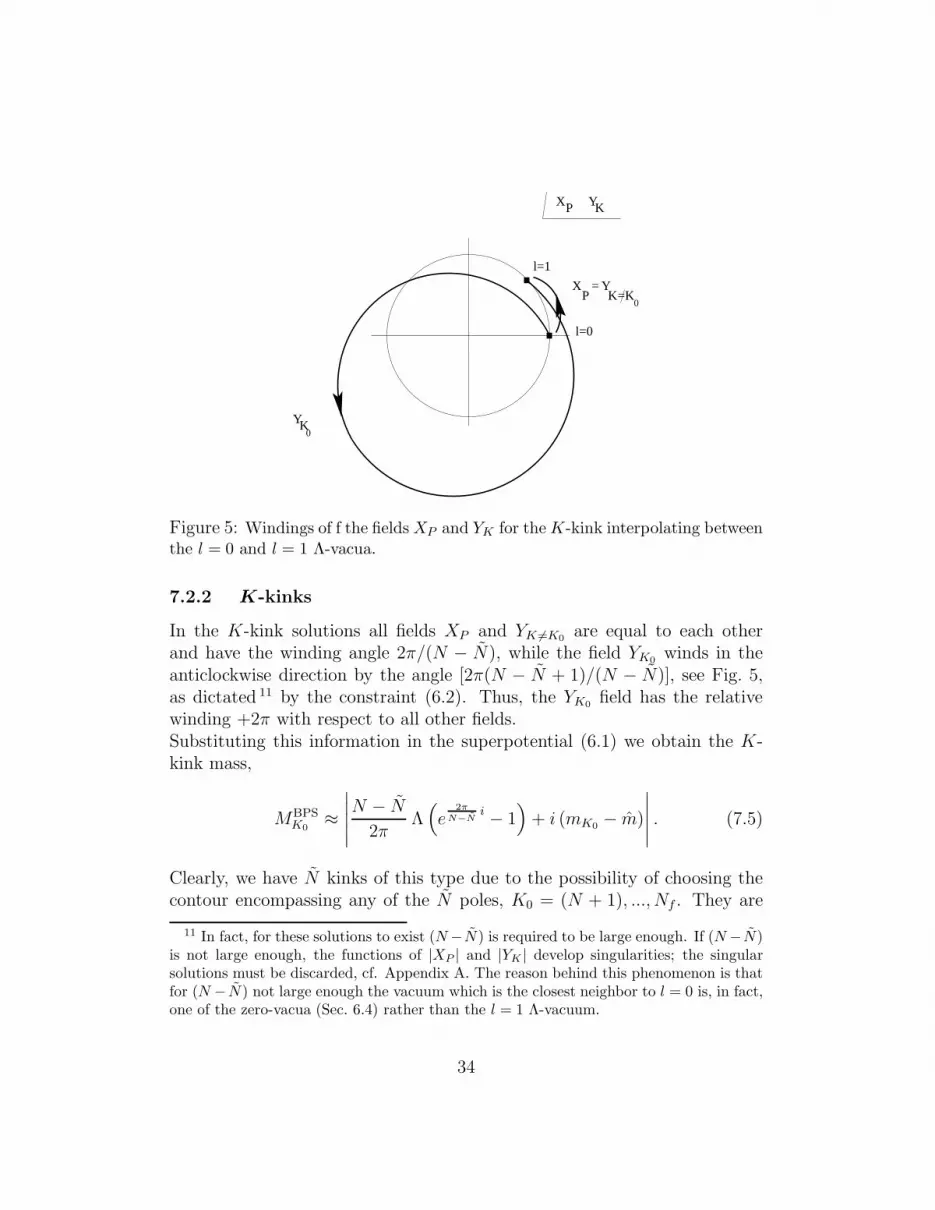
Figure 5: Windings of f the fieldsXP and YK for theK-kink interpolating betweenthe l = 0 and l = 1 Λ-vacua.

7.2.2 K-kinks

In the K-kink solutions all fields XP and YK 6=K0are equal to each other

and have the winding angle 2π/(N − N), while the field YK0winds in the

anticlockwise direction by the angle [2π(N − N + 1)/(N − N)], see Fig. 5,as dictated 11 by the constraint (6.2). Thus, the YK0

field has the relativewinding +2π with respect to all other fields.Substituting this information in the superpotential (6.1) we obtain the K-kink mass,

MBPSK0

≈∣∣∣∣∣N − N

2πΛ(e

2π

N−Ni − 1

)+ i (mK0

− m)

∣∣∣∣∣ . (7.5)

Clearly, we have N kinks of this type due to the possibility of choosing thecontour encompassing any of the N poles, K0 = (N + 1), ..., Nf . They are

11 In fact, for these solutions to exist (N−N) is required to be large enough. If (N−N)is not large enough, the functions of |XP | and |YK | develop singularities; the singularsolutions must be discarded, cf. Appendix A. The reason behind this phenomenon is thatfor (N − N) not large enough the vacuum which is the closest neighbor to l = 0 is, in fact,one of the zero-vacua (Sec. 6.4) rather than the l = 1 Λ-vacuum.

34

split at generic masses, but become degenerate in the limit (2.5). They formthe fundamental representation of the global SU(N) group in this limit.

Altogether we have Nf kinks interpolating between each pair of neigh-boring Λ-vacua. They form the fundamental representation of the globalgroup (2.12) in the limit (2.5). More exactly, they form the (N, 1) + (1, N)representation of this group.

Much in the same way as in the CP(N − 1) model, we can verify thatEq. (5.8) reproduces this spectrum with the appropriate choice of the integra-tion contours. Namely, for the P0-kink the contour in the σ plane encirclesthe pole at

√2σ = −mP0

in the clockwise direction, see Fig. 4. For theK0-kink the contour encircles the pole at

√2σ = −mK0

in the anticlockwisedirection.

7.3 Kinks in the zero-vacua

Now we consider kinks in the zero-vacua in the domain of small hierarchicalmasses (5.7). These vacua of the weighted CP model are most interestingsince they correspond to N non-Abelian strings of the dual bulk theory.Clearly, the number of kinks does not depend on which pair of neighboringvacua we pick up. Thus, we expect to have altogether Nf kinks, as was thecase in the Λ-vacua. We check this explicitly below.

Much in the same way as in the Λ-vacua, the kinks interpolating betweenthe neighboring l = 0 and l = 1 zero-vacua (see (6.17)) fall into two cat-egories: the P - and K-kinks, respectively, depending on the choice of theparticular XP0

or YK0field with an opposite winding with respect to other

fields.

7.3.1 K-kinks

Let us start from the K-kinks. The kink solution looks very similar to thatin the CP(N − 1) model. All YK 6=K0

fields are approximately equal to eachother and have the winding angles 2π/N , while the YK0

field has the windingangle −2π(N − 1)/N , see (6.17). Correction terms in XP , proportional toΛLE/Λ also all have the same windings by the angle 2π/N , see (6.19). Thisgives the following expression for the mass of the K0-kink:

MBPSK0

≈∣∣∣∣∣N − N

2πΛLE

(e

2π

Ni − 1

)− i (mK0

− m)

∣∣∣∣∣ . (7.6)

35

The factor (N−N) in the first term appears from two first terms in (6.1) dueto winding of both XP and YK fields. The imK0

term is due to the relativewinding −2π of the YK0

field.We have N kinks of this type associated with the arbitrary choice of K0 =

(N + 1), ..., Nf . They are split with generic masses, but become degeneratein the limit (2.5). In this limit they form the fundamental representation ofthe global SU(N) group.

7.3.2 P -kinks

In this case all YK fields are approximately equal to each other and have thewinding angles 2π/N . The fields XP 6=P0

are all equal to ∆m/Λ, to the leadingorder, and do not wind; however, they have windings 2π/N in the correctionterms, see (6.19). The field XP0

does wind. Its absolute value is ∆m/Λ .The winding angle is 2π, as enforced by the constraint (6.2), see Fig. 6. Amore detailed description of the kink solutions is presented in Appendix B.The windings above imply the following mass of the P0-kink:

MBPSP0

≈∣∣∣∣∣N − N

2πΛLE

(e

2π

Ni − 1

)− i (mP0

− m)

∣∣∣∣∣

=

∣∣∣∣∣−i∆m +N − N

2πΛLE

(e

2π

Ni − 1

)− i (mP0

−m)

∣∣∣∣∣ , (7.7)

where m and m are given by (6.10) and (6.18), while ∆m = m−m, see (4.6).In the last expression the first term is the leading contribution, the secondone is a correction, while the third term accounts for still smaller splittings.

There are N kinks of this type associated with the arbitrary choice ofP0 = 1, ..., N . They are split at generic masses, but become degeneratein the limit (2.5). They form the fundamental representation of the globalSU(N) group in this limit.

Much in the same way as in the Λ-vacua, the total number of the kinksinterpolating between each pair of the neighboring zero-vacua is Nf . Theyform the (N, 1)+(1, N) representation of the global group (2.12) in the limit(2.5). Note, that the P -kinks in the zero-vacua are heavier than the K-kinks.Their masses are given by ∆m (to the leading order) while theK-kink massesare of the order of ΛLE . Still, given small hierarchical masses (5.7), all kinks

36

l=1

l=0

YK

YKXP

XP0

m∆Λ LE ΛΛ

Figure 6: Windings of fields XP0and YK for the P0-kink interpolating between

l = 0 and l = 1 zero-vacua.

in the zero-vacua are lighter than those in the Λ-vacua which have masses ofthe order of Λ, see Eqs. (7.4) and (7.5).

In parallel with the Λ-vacua, we can verify that Eq. (5.8) reproduces theabove BPS spectrum with the appropriate choice of the integration contours.Namely, for the P0-kink the contour in the σ plane encircles the pole at√2σ = −mP0

in the anticlockwise direction, cf. Fig. 4. For the K0-kink thecontour encircles the pole at

√2σ = −mK0

in the clockwise direction.

8 Lessons for the bulk theory

This section carries a special weight and is, in a sense, central for the presentinvestigation, since here we translate our results for the kink spectrum inthe weighted two-dimensional CP model (3.2) in the language of strings andconfined monopoles of the bulk four-dimensional theory.

We start from the most interesting strong-coupling domain

ξ ≪ Λ (8.1)

which can be described in terms of weakly-coupled dual bulk theory [11], seeSec. 2.2. At this point we take the limit (2.5) to ensure the presence of theunbroken global group (2.12).

37

As was mentioned previously, the elementary non-Abelian strings of thebulk theory correspond to various vacua of the world-sheet two-dimensionaltheory, see, e.g. the review paper [19] for a detailed discussion. The weightedCP model (3.9) has two types of vacua, namely: (N − N) Λ-vacua and Nzero-vacua. The former are not-so-interesting from the standpoint of thebulk theory. Indeed, they yield just Abelian ZN−N strings associated with the

winding of the (N−N) singlet dyons Dl charged with respect to U(1) factorsof the gauge group of the dual theory (2.10) [11], see (2.11). Moreover, theweighted CP model (3.9) is, in fact, inapplicable in the description of thesestrings. This model is an effective low-energy theory which can be used belowthe scale

√ξ. However, the energy scale in the Λ-vacua is of order of Λ, i.e.

much larger than√ξ in the domain (8.1).

Below we focus on N zero-vacua which correspond to N elementary non-Abelian strings associated with the winding of the light dyons DlA of thedual bulk theory. The latter are charged with respect to both Abelian andnon-Abelian factors [11] of the dual gauge group (2.10). The energy scale inthese vacua of the world-sheet theory is of the order of

max(∆mKK ′, ΛLE) ,

which we assume to be much less than√ξ. Thus, in these vacua the weighted

CP model (3.9) can be applied to describe the internal dynamics of the non-Abelian strings of the bulk theory.

The confined monopoles of the bulk theory are seen as kinks in the world-sheet theory. The results presented in Sec. 7 demonstrate that in the weightedCP model there are Nf elementary kinks interpolating between the neigh-boring zero-vacua. More exactly, we found N P -kinks with masses (7.7) andN K-kinks with masses (7.6). In the limit (2.5) they form the (N, 1)+(1, N)representations of the global group (2.12).

This means that the total number of stringy mesons MBA formed by the

monopole-antimonopole pairs connected by two different elementary non-Abelian strings (Fig. 1) is N2

f . The mesons MP ′

P form the singlet and(N2 − 1, 1) adjoint representations of the global group (2.12), the mesons

MKP and MP

K form bifundamental representations (N, ¯N) and (N, N), whilethe mesons MK ′

K form the singlet and (1, N2 − 1) adjoint representations.(Here as usual, P = 1, ..., N and K = (N+1), ..., Nf .) All these mesons havemasses of the order of

√ξ, determined by the string tension

T = 2πξ . (8.2)

38

They are heavier than the elementary states, namely, dyons and dual gauge

bosons which form the (1,1), (N, ¯N), (N, N), and (1, N2−1) representationsand have masses ∼ g2

√ξ.

Therefore, the (1,1), (N, ¯N), (N, N), and (1, N2 − 1) stringy mesonsdecay into elementary states, and we are left with MP ′

P stringy mesons inthe representation (N2 − 1, 1). This is exactly what was predicted in [11]from the bulk perspective, see Sec. 2.2. Thus, our world sheet picture nicelymatches the bulk analysis.

Note also that the MP ′

P stringy mesons with strings corresponding to theΛ-vacua of the weighted CP model (the “Λ-strings”) are heavy and decayinto MP ′

P stringy mesons with strings corresponding to the zero-vacua (the“zero-strings”). To see that this is indeed the case, observe that the confinedmonopoles (i.e. kinks of the weighted CP model) on the Λ-string have massesof the order of Λ, see (7.4). Therefore, the Λ-stringy mesons also have massesof the order of Λ. The MP ′

P mesons with the zero-strings are much lighter inthe domain (8.1). Their masses are of the order of max(∆m,

√ξ).

Now, let us discuss yet another match of the world-sheet and bulk pic-tures. In Sec. 5.1 we saw that there are elementary excitations (T = 0 andSA = δAP1

−δAP2) on the string at weak coupling (this is attainable with large

|∆mAB|). These excitations would form the adjoint representation (N2−1, 1)of the global group if the limit (2.5) could be taken. However, in the strongcoupling domain of hierarchically small masses (5.7) the kink spectrum isvery different, see Sec. 7. In particular, no elementary excitations are left:these states decay on CMS into a P1-kink plus a P2-antikink, see Eqs. (7.4)and (7.7).

Since the BPS spectra of the N = (2, 2) two-dimensional theory on thestring and the N = 2 four-dimensional bulk theory on the Coulomb branch(at zero ξ) coincide [26, 27, 15, 16], the decay process above is in one-to-onecorrespondence with the decay of the bulk states identified in [11]. Namely,the quarks qkP1 (with k = P2 due to the color-flavor locking) and the gaugebosons present in the bulk theory at weak coupling decay into monopole-antimonopole pairs. If ξ is small but nonvanishing, the monopoles and anti-monopoles cannot move apart: they are bound together by pairs of confiningstrings and form [11] the MP1

P2mesons shown in Fig. 1. Thus, our results

from two dimensions confirm the decay of the quarks and gauge bosons inthe strong-coupling domain of the bulk theory. This decay process is a crucialelement of our mechanism of non-Abelian confinement.

39

ξ

Λ

Λ2

∆ m ∆ m KK’Λ LE

ΛLE2

C

B

ED

F

A

PP’

Figure 7: “Phase diagram” of the bulk theory. Various domains are separated byCMS on which physical spectrum is rearranged.

To explain this in more detail we present a “phase diagram” of the bulktheory, see Fig. 7. The vertical and horizontal solid lines in this figureschematically represent the bulk theory CMS. The horizontal axis gives themasses ∆mPP ′ ∼ ∆mKK ′ which we force to be of the same order, while ∆mis fixed, ∆m ≪ Λ. The vertical axis gives the FI parameter ξ. The verti-cal dashed lines depict CMS of the world-sheet theory. On these lines thespectrum of the stringy mesons of the bulk theory rearranges itself. On thesolid lines the “perturbative” spectrum of the bulk theory rearranges itself.Different domains inside CMS (where the spectra change continuously) aredenoted by capital letters A, B, ..., F.

The domains A, B and C are at weak coupling in the original U(N)gauge theory. The elementary (“perturbative”) states in these domains arethe qkA quarks and gauge bosons of the U(N) gauge group. The domains Dand E are at weak coupling in the dual theory, see Sec. 2.2. The elementary(“perturbative”) states in these domains are the light dyons DlA and Dl inEq. (2.11) plus the gauge bosons of the dual gauge group (2.10). Masses ofall these states smoothly evolve with the change of parameters inside thesedomains. The domain F is at strong coupling in the dual theory. Withsmall mass differences in the domain (5.7), N flavors of dyons in Eq. (2.11)decouple, the dual theory becomes asymptotically free, and at ξ ≪ ΛLE

passes into the strong coupling regime. The dual gauge group (2.10) gets

40

broken down to U(1)N by the Seiberg–Witten mechanism.Keeping in mind the limit (2.5), our task is to pass from the domain A

into the domain D and prove that the quarks and gauge bosons of the formerdomain decay into the monopole-antimonopole pairs connected by confiningstrings in the domain D. We do it in three steps. First, we pass from thedomain A to C at large ξ and then move towards small ξ (preserving largemass differences) inside C. The original bulk theory is in the weak-couplingregime in these domains and the quarks and gauge boson spectra evolvesmoothly.

Next, we pass from the domain C to the domain E at small (or vanishing)ξ. Here we use correspondence between the BPS spectra of the bulk andworld-sheet theories. The qkP1 quarks (with k = P2 due to the color-flavorlocking) and gauge bosons of the domain C correspond to elementary stateswith T = 0 and SA = δAP1

− δAP2, see (4.2). As was already explained, these

states decay on CMS of the two-dimensional theory into a P1-kink and aP2-antikink, interpolating between the Λ-vacua, see (7.4). Since the spectraof the massive BPS states in the bulk (at ξ = 0) on the one hand, and inthe world-sheet theory on the other hand, are identical, both the quarks andgauge bosons from domain C do not exist in the domain E. They decayinto a P1-monopole and a P2-antimonopole. At small but nonvansishing ξthe latter states are confined by Λ-strings which gives rise to MP1

P2stringy

mesons.Furthermore, as we pass from the domain E to our final destination –

the domain D – these MP1

P2mesons “glued” by Λ-strings, decay on the world-

sheet theory CMS located at ∆mPP ′ ∼ ∆mKK ′ ∼ ΛLE. They decay intolighter MP1

P2mesons glued by zero-strings. The latter stringy mesons were

absent in the domain E at intermediate masses (see (5.20)), but emerge inthe domain D at small masses, see (7.7). This completes our proof.

In conclusion it is worth noting that the stringy mesonsMP ′

P in the adjointrepresentation (N2 − 1, 1) of the global group are metastable, strictly speak-ing. An extra monopole-antimonopole pair can be created on the string, mak-ing the (N2−1, 1) meson to decay into a pair of stringy mesons in the bifun-

damental representation, (N, ¯N) and (N , N). During the subsequent stagethese stringy bifundamentals decay into elementary bifundamental dyons.One can suppress the rate of this decay, however. If we keep ∆m ≪ √

ξand take a limit of large N , while N is fixed this decay rate is of the orderof N/N ≪ 1. To see that this indeed the case, note that the above de-

41

cay process goes through creation of a monopole-antimonopole pair from thefundamental representation of SU(N) on the string which selects N channelsout of Nf .

Similar considerations can be applied to the weak-coupling domain oflarge ξ, √

ξ ≫ Λ ,

of the bulk theory. We still have kinks in the (N, 1) + (1, N) representationsof the global group (2.4) in the limit (2.5). Thus, all types of mesons MA

B

are formed with masses ∼ √ξ. However, in this regime the (1,1), (N, ¯N),

(N, N), and (N2 − 1, 1) stringy mesons can decay into quarks and gaugebosons with the same quantum numbers and masses ∼ g22

√ξ. Therefore, we

are left with elementary states and stringy adjoint mesons (1, N2 − 1). Thelatter are metastable and decay in pairs of bifundamental states.

9 Conclusions

Both N = 2 four-dimensional theories belonging to the dual pair discussedabove support non-Abelian strings. The world-sheet theory on the strings isgiven by the weighted CP model which appears in two varieties depending onwhich side of duality we are. These two weighted CP models also form a dualpair. We explore the kink spectra (which represent confined monopoles of thebulk theory) and their evolution in passing through the crossover domain.Of most interest is small-ξ dynamics. In fact, at small ξ we find two weakcoupling subdomains and a strong-coupling one depending on the values ofthe differences of the mass parameters ∆mAB.

We have shown that in the limit (2.5) where the global group (2.4) isunbroken confined monopoles form the fundamental representation of theglobal group. Therefore, stringy mesons (shown in Fig. 1) formed by pairs ofmonopoles and antimonopoles belong to the adjoint or singlet representationsof the global group. This nicely matches global quantum numbers of mesonsin the “real world.”

We proved the statement proposed in [11] that quarks and gauge bosonspresent in the original theory at large ξ decay on CMS into monopole-antimonopole pairs confined by non-Abelian strings as we enter the small-ξdomain. This result is a crucial element of our mechanism of non-Abelianconfinement.

42

In summary, in this paper we used the world-sheet theory to confirm thepicture of non-Abelian confinement obtained in [11] from the bulk perspec-tive. Non-Abelian confinement is not associated with formation of chromo-electric strings connecting quarks, as a naive extrapolation of the Abelianconfinement picture suggests. Rather, it is due to the decay on CMS of theHiggs-screened quarks and gauge bosons into monopole-antimonopole pairsconfined by non-Abelian strings in the strong coupling domain of small ξ.We stress again that the non-Abelian strings confine monopoles both in theoriginal and dual theories.12

Analysis of the mass spectra presented in the bulk of the paper raises anumber of intriguing questions. One of them refers to typical sizes of theobjects considered. At the moment, in the absence of a detailed analysis,one can address this issue only at the qualitative level. At small ξ and∆m ≪ √

ξ ≪ Λ we expect that the smallest size ∼ Λ−1 is that of theelementary (“perturbative”) states, namely dyons from Eq. (2.11) and dualgauge bosons. The sizes of the stringy mesons in the representation N2 − 1are expected to be of the order (g

√ξ)−1, i.e of order of the thickness of the

non-Abelian strings. Finally, the largest sizes (∆m)−1 and ∼ Λ−1LE belongs to

the P - and K-kinks (confined monopoles on a string), respectively, providedthat the mass difference ∆mKK ′ → 0.

Acknowledgments

We are grateful to A. Gorsky for valuable discussions.This work is supported in part by DOE grant DE-FG02-94ER408. The

work of A.Y. was supported by FTPI, University of Minnesota, by RFBRGrant No. 09-02-00457a and by Russian State Grant for Scientific SchoolsRSGSS-11242003.2.

12 Similar results were recently obtained in [46] for N = 2 supersymmetric QCD withNf > 2N .

43

Appendix A:

Kink solutions in CP(N − 1) model

In this appendix we discuss in more detail the kink solutions in the CP(N − 1)model (see Sec. 7.1). For simplicity we set ∆mPP ′ = 0. Small mass differ-ences will slightly deform the kink profile functions but will not change thevery fact of its existence. The kink masses are given by differences of themirror superpotential evaluated at the initial and final vacua, see (7.2).

We look for the kink solution interpolating between l = 0 and l = 1 vacuausing the ansatz

XP 6=P0= r eiθ, XP0

=e−i(N−1)θ

r(N−1), (A.1)

where r(z) and θ(z) are kink profile functions, subject to boundary conditions

θ(z = −∞) = 0, r(z = −∞) = 1,

θ(z = ∞) =2π

N, r(z = ∞) = 1, (A.2)

see (6.9). The last expression in (A.1) is dictated by (6.7).The explicit form of the kink profile functions depends on the form of

the kinetic term which is not known. Therefore, both profile functions r(z)and θ(z) cannot be determined. Still we can obtain the kink solution upto a single unknown profile function θ(z) expressing r as a function of θ.To this end we exploit the fact that the kink trajectory in the complexplane of superpotential goes along the straight line connecting the pointsWmirror(l = 0) with Wmirror(l = 1) [38]. The difference

Wmirror(l = 1)−Wmirror(l = 0) = −NΛ

4π

(e

2πN

i − 1)

= −NΛ

4πe

πN

i 2i sin( π

N

), (A.3)

where we used (6.6) and (6.9).

44

On the other hand,

Wmirror(θ)−Wmirror(θ = 0) = − Λ

4π

[(N − 1)reiθ +

1

rN−1e−i(N−1)θ −N

]

= −rΛ

4πe

πN

i

{(N − 1)ei(θ−

πN) +

1

rNe−i(N−1)θ−i π

N − N

re−

πN

}. (A.4)

Comparing Eqs. (A.3) and (A.4) we see that for the kink trajectory to goalong the straight line, the real part of the expression in the curly bracketsin (A.4) must vanish. As a result,

(N − 1) cos(θ − π

N

)− N

rcos

π

N+

1

rNcos[(N − 1)θ +

π

N

]= 0. (A.5)

This equation determines the function r(θ). It has a nonvansihing nonsin-gular solution at 0 ≤ θ ≤ 2π/N which satisfies the boundary conditionsr(2π/N) = r(0) = 1. Say, for N = 2, r = 1. For large N the profile functionr is approximately given by

r(θ) ≈ 1 +1

N

{1− cos

[(N − 1)θ +

π

N

]}+ · · · . (A.6)

Appendix B:

Kink solutions in the zero-vacua

Here we consider the kink solutions interpolating between the zero-vacua withl = 0 and l = 1, see (6.17), at hierarchically small masses (5.7). The K-kinksolutions in the zero-vacua are quite similar to kinks in the CP(N−1) model.Therefore, we focus on P -kinks.

Analyzing the P -kinks we assume the limit (2.5) (for simplicity). Theansatz for the kink solution takes the form

YK = r eiθΛLE

Λ,

XP 6=P0≈ ∆m

Λ, XP0

≈ ∆m

ΛrNeiNθ , (B.1)

where we restrict ourselves to the leading order contributions (∼ ∆m/Λ)ignoring next-to-leading O(ΛLE/Λ) terms. The profile functions r(z) and

45

������������

������������

1

1

−1

l.h.s.

r.h.s.

r

Figure 8: The right- and left-hand sides of Eq. (B.5). The closed circle denotesthe regular solution.

θ(z) are subject to the boundary conditions

θ(z = −∞) = 0, r(z = −∞) = 1 ,

θ(z = ∞) =2π

N, r(z = ∞) = 1 , (B.2)

see (6.17) and (6.15). The last expression in (B.1) is dictated by (6.2).The superpotential (6.1) then gives

Wmirror(θ)−Wmirror(θ = 0)

≈ −∆m

4π

{rNeiNθ − N (iθ + ln r)− 1

}, (B.3)

while the difference of the superpotential in the initial and final vacua is

Wmirror(l = 1)−Wmirror(l = 0) ≈ ∆m

4π× 2πi . (B.4)

For the kink trajectory to go along the straight line in the complex plane ofsuperpotential, the real part of the expression in the curly brackets in (B.3)must vanish. This requirement implies

rN cos (Nθ)− N ln r = 1 . (B.5)

46

The latter equation always has a finite nonvanishing solution in the interval0 ≤ θ ≤ 2π/N , subject to the boundary conditions r(2π/N) = r(0) = 1. Tocheck that this is indeed the case we rewrite it as

cos (Nθ) =1 + N ln r

rN. (B.6)

The right- and left-hand sides of (B.6) are schematically plotted in Fig. 8.For any −1 < cos (Nθ) < 1 we have only one nonsingular solution r(θ). Inparticular, at N ≫ 1

r(θ) ≈ 1− 1

N[1− cos (Nθ)] + · · · . (B.7)

47

References

[1] Y. Nambu, Phys. Rev. D 10, 4262 (1974);G. ’t Hooft, Gauge theories with unified weak, electromagnetic and strong in-

teractions, in Proc. of the E.P.S. Int. Conf. on High Energy Physics, Palermo,23-28 June, 1975 ed. A. Zichichi (Editrice Compositori, Bologna, 1976); Nucl.Phys. B 190, 455 (1981); S. Mandelstam, Phys. Rept. 23, 245 (1976).

[2] A. Abrikosov, Sov. Phys. JETP 32, 1442 (1957) [Reprinted in Solitons and

Particles, Eds. C. Rebbi and G. Soliani (World Scientific, Singapore, 1984),p. 356]; H. Nielsen and P. Olesen, Nucl. Phys. B61, 45 (1973) [Reprintedin Solitons and Particles, Eds. C. Rebbi and G. Soliani (World Scientific,Singapore, 1984), p. 365].

[3] N. Seiberg and E. Witten, Nucl. Phys.B426, 19 (1994), (E) B430, 485 (1994)[hep-th/9407087].

[4] N. Seiberg and E. Witten, Nucl. Phys. B431, 484 (1994) [hep-th/9408099].

[5] A. M. Polyakov, Nucl. Phys. B 120, 429 (1977).

[6] M. R. Douglas and S. H. Shenker, Nucl. Phys. B 447, 271 (1995)[hep-th/9503163].

[7] A. Hanany, M. J. Strassler and A. Zaffaroni, Nucl. Phys. B 513, 87 (1998)[hep-th/9707244].

[8] M. Strassler, Prog. Theor. Phys. Suppl. 131, 439 (1998) [hep-lat/9803009].

[9] A. I. Vainshtein and A. Yung, Nucl. Phys. B 614, 3 (2001) [hep-th/0012250].

[10] A. Yung, What Do We Learn About Confinement From The Seiberg–Witten

Theory?, Proc. of 28th PNPIWinter School of Physics, St. Petersburg, Russia,2000, [hep-th/0005088]; published in At the frontier of particle physics, Ed.M. Shifman, (World Scientific, Singapore, 2001) vol. 3, p. 1827.

[11] M. Shifman and A. Yung, Phys. Rev. D 79, 125012 (2009) [arXiv:0904.1035[hep-th]].

[12] P. Fayet and J. Iliopoulos, Phys. Lett. B 51, 461 (1974).

[13] A. Hanany and D. Tong, JHEP 0307, 037 (2003) [hep-th/0306150].

[14] R. Auzzi, S. Bolognesi, J. Evslin, K. Konishi and A. Yung, Nucl. Phys. B673, 187 (2003) [hep-th/0307287].

[15] M. Shifman and A. Yung, Phys. Rev. D 70, 045004 (2004) [hep-th/0403149].

[16] A. Hanany and D. Tong, JHEP 0404, 066 (2004) [hep-th/0403158].

[17] D. Tong, TASI Lectures on Solitons, arXiv:hep-th/0509216.

[18] M. Eto, Y. Isozumi, M. Nitta, K. Ohashi and N. Sakai, J. Phys. A 39, R315(2006) [arXiv:hep-th/0602170].

48

[19] M. Shifman and A. Yung, Supersymmetric Solitons, Rev. Mod. Phys. 79 1139(2007) [arXiv:hep-th/0703267]; an expanded version in Cambridge UniversityPress, 2009.

[20] D. Tong, Annals Phys. 324, 30 (2009) [arXiv:0809.5060 [hep-th]].

[21] M. Shifman and A. Yung, Phys. Rev. D 79, 105006 (2009) arXiv:0901.4144[hep-th].

[22] M. Shifman and A. Yung, Non-Abelian Strings: From Weak to Strong Cou-

pling and Back via Duality, arXiv:0910.3007 [hep-th].

[23] P. Argyres, M. Plesser and N. Seiberg, Nucl. Phys. B471, 159 (1996)[hep-th/9603042].

[24] N. Seiberg, Nucl. Phys. B 435, 129 (1995) [arXiv:hep-th/9411149].

[25] K. A. Intriligator and N. Seiberg, Nucl. Phys. Proc. Suppl. 45BC, 1 (1996)[hep-th/9509066].

[26] N. Dorey, JHEP 9811, 005 (1998) [hep-th/9806056].

[27] N. Dorey, T. J. Hollowood and D. Tong, JHEP 9905, 006 (1999)[arXiv:hep-th/9902134].

[28] A. Achucarro and T. Vachaspati, Phys. Rept. 327, 347 (2000)[hep-ph/9904229].

[29] M. Shifman and A. Yung, Phys. Rev. D 73, 125012 (2006)[arXiv:hep-th/0603134].

[30] M. Eto, J. Evslin, K. Konishi, G. Marmorini, M. Nitta, K. Ohashi, W. Vinci,N. Yokoi, Phys. Rev. D 76, 105002 (2007) [arXiv:0704.2218 [hep-th]].

[31] E. Witten, Nucl. Phys. B 149, 285 (1979).

[32] K. Hori and C. Vafa, Mirror symmetry, arXiv:hep-th/0002222.

[33] A. Bilal and F. Ferrari, Nucl. Phys. B 516, 175 (1998) [arXiv:hep-th/9706145].

[34] D. Tong, Phys. Rev. D 69, 065003 (2004) [hep-th/0307302].

[35] E. Witten, Nucl. Phys. B 403, 159 (1993) [hep-th/9301042].

[36] K. Evlampiev, A. Yung, Nucl. Phys. B 662, 120 (2003) [hep-th/0303047].

[37] A. D’Adda, A. C. Davis, P. DiVeccia and P. Salamonson, Nucl. Phys. B222

45 (1983).

[38] S. Cecotti and C. Vafa, Comm. Math. Phys. 158 569 (1993).

[39] G. Veneziano and S. Yankielowicz, Phys. Lett. B 113, 231 (1982).

[40] A. Hanany and K. Hori, Nucl. Phys. B 513, 119 (1998)[arXiv:hep-th/9707192]. [hep-th/9211097].

[41] M. Shifman, A. Vainshtein and R. Zwicky, J. Phys. A 39, 13005 (2006)[arXiv:hep-th/0602004].

49

[42] S. Olmez and M. Shifman, J. Phys. A 40, 11151 (2007) [hep-th/0703149]

[43] S. Lee, P. Yi, A Study of Wall-Crossing: Flavored Kinks in D=2 QED,arXiv:0911.4726 [hep-th].

[44] V. A. Fateev, I. V. Frolov and A. S. Schwarz, Sov. J. Nucl. Phys. 30, 590(1979) [Yad. Fiz. 30, 1134 (1979)]; Nucl. Phys. B 154 (1979) 1. See also inA. Polyakov, Gauge Fields and Strings (Harwood Press, 1987).

[45] A. Ritz, M. Shifman and A. Vainshtein, Phys. Rev. D 66, 065015 (2002)[hep-th/0205083].

[46] A. Marshakov and A. Yung, Strong versus weak coupling confinement in N =2 supersymmetric QCD, arXiv:0912.1366 [hep-th].

50