arX

iv:h

ep-t

h/97

0800

4v2

24

Oct

199

7

hep-th/9708004

ITFA-97-28

Quantisation of monopoles with

non-abelian magnetic charge

F.A. Bais† and B.J. Schroers‡

Instituut voor Theoretische Fysica

Universiteit van Amsterdam

Valckenierstraat 65, 1018 XE Amsterdam

The Netherlands

Abstract

Magnetic monopoles in Yang-Mills-Higgs theory with a non-abelian unbroken gauge groupare classified by holomorphic charges in addition to the topological charges familiar fromthe abelian case. As a result the moduli spaces of monopoles of given topological chargeare stratified according to the holomorphic charges. Here the physical consequences of thestratification are explored in the case where the gauge group SU(3) is broken to U(2). Thedescription due to A. Dancer of the moduli space of charge two monopoles is reviewed andinterpreted physically in terms of non-abelian magnetic dipole moments. Semi-classicalquantisation leads to dyonic states which are labelled by a magnetic charge and a repre-sentation of the subgroup of U(2) which leaves the magnetic charge invariant (centralisersubgroup). A key result of this paper is that these states fall into representations of thesemi-direct product U(2) ⋉ R4. The combination rules (Clebsch-Gordan coefficients) ofdyonic states can thus be deduced. Electric-magnetic duality properties of the theory arediscussed in the light of our results, and supersymmetric dyonic BPS states which fill theSL(2,Z)-orbit of the basic massive W -bosons are found.

to appear in Nuclear Physics B

† e-mail: bais@phys.uva.nl‡ e-mail: schroers@phys.uva.nl

1. Introduction

The study of magnetic monopole solutions in spontaneously broken gauge theories,

sparked off more than twenty years ago by ’t Hooft’s and Polyakov’s discovery of the

eponymous monopole solution in SU(2) Yang-Mills-Higgs theory [1], has progressed from

the classification and in some cases explicit construction of monopoles via the description

of the spaces of solutions (the moduli spaces) to, more recently, the discussion of classical

and quantised dynamics of monopoles. Perhaps not surprisingly, most progress has been

made in the theory originally considered by ’t Hooft and Polyakov where, in a special limit

called the BPS limit, the understanding of the geometry of the classical moduli spaces could

be used rigorously to establish the existence of infinitely many (supersymmetric) quantum

bound states of magnetic monopoles [2][3]. These bound states, which are typically dyonic,

are related to the electrically charged W -bosons of the theory via electric-magnetic duality

or S-duality and their existence confirms the possibility of formulating Yang-Mills theory in

infinitely many equivalent ways, all related by S-duality and each having different particles

as fundamental degrees of freedom.

As far as the spectrum of magnetically and electrically charged particles is concerned

the step from Yang-Mills-Higgs theory with gauge group SU(2) broken to U(1) to a general

gauge group G broken to some subgroup H is not of great qualitative difficulty provided

the group H is abelian. Indeed, in the case G = SU(N) and H = U(1)N−1 (a maximal

torus of G) much is known about monopole solutions, their moduli spaces, their quantum

bound states and the action of electric-magnetic duality, even quantitatively [4]. When

H is non-abelian, however, it was already pointed out more than ten years ago by a

number of authors that qualitatively new problems arise when attempting physically to

interpret parameters of multimonopole solutions and when discussing dyonic excitations

of monopoles. The many interesting physical problems unearthed by these discussions,

however, were largely ignored in the more mathematical treatment of monopoles and their

moduli spaces in recent years. In attempting the final of the steps outlined above, that

of trying to apply the mathematical understanding of monopole moduli spaces to the

study of classical and quantum dynamics of monopoles, these problems naturally return.

In particular they beset any attempt of understanding electric-magnetic duality in these

theories. Let us therefore briefly review the issues involved.

The allowed values of magnetic charges in non-abelian gauge theories are restricted by

the generalised Dirac quantisation condition see [5], [6], and also [7]. A naive application

of this condition leads to the representation of the allowed magnetic charges as points on

the dual of the weight lattice of the full gauge group G. Thus, if we denote the rank

of G by R, magnetic charges correspond to vectors in a R-dimensional lattice, usually

called magnetic weight vectors. This general condition does not reflect the specifics of the

symmetry breaking. On the other hand there is a topological classification of magnetic

charges which depends crucially on the breaking of G down to the exact residual gauge

group H. The topological charges are elements of the second homotopy group Π2(G/H)

(= Π1(H) if G is simply connected) and thus depend strongly on the connectedness of

H. If one breaks the symmetry to a maximal torus H ∼= U(1)R of G (maximal symmetry

breaking) the classification resulting from the Dirac condition agrees with the topological

classification: all R components of the magnetic weight vectors are topologically conserved.

Now consider the degenerate situation where one does not break maximally and the exact

group H is non-abelian. The magnetic weight vectors now have more components than

the number of topologically conserved charges, raising the question of which - if any -

relevance the remaining components (called the non-abelian components) might have. The

answer is rather subtle and depends on additional assumptions. If one carries the Brandt-

Neri reasoning [8] over to the unbroken group H one might expect that configurations

whose magnetic weight vectors have non-abelian components will decay to configurations

whose non-abelian components are, in a suitable sense, minimal. There is no topological

obstruction to doing so. However, if one considers the theory in the BPS limit, shedding

non-abelian charge in this way does not lower the energy. Mathematical analysis has

revealed that there are neutrally stable solutions which have magnetic weights with non-

minimal non-abelian components (restricted to lie in a certain range). In this situation the

magnetic weights regain some of their glory. Mathematically they characterise holomorphic

properties of the solution and they (or more precisely certain equivalence classes of them)

are called holomorphic charges in the mathematical literature. Thus one may say that in

general the magnetic weight vectors have topological and holomorphic components.

To illustrate the general discussion consider the simplest non-trivial example where

G = SU(3) and H = U(1)×U(1) or H = U(2) for, respectively, maximal or minimal sym-

metry breaking. In Fig. 1 we show the magnetic weight lattice, spanned by the two simple

roots ~β1 and ~β2, together with the direction ~h of the Higgs field which determines the sym-

metry breaking pattern. For each point in the weight lattice we indicate the dimensionality

of the corresponding space of monopole solutions, called moduli space and to be defined

more precisely in the main part of the paper. In the case of maximal symmetry breaking

there are non-trivial moduli spaces for all positive magnetic weights (there are also moduli

spaces for negative magnetic weights, containing anti-monopoles, but we do not consider

these here). In the case of minimal symmetry breaking non-trivial moduli spaces only

occur inside the cone shown in Fig. 1.b, where the topological component of the magnetic

weight vectors is plotted vertically and the holomorphic component horizontally. The ge-

ometrical structure of these spaces is intricate. Each topological sector corresponds to a

connected moduli space which consists of different strata of varying dimensions, with each

stratum labelled by an (integer) holomorphic charge. There are one-parameter families of

solutions where the holomorphic charge jumps from one discrete value to the next as the

parameter varies continuously. These mathematical facts have so far not been interpreted

physically. What is the physical meaning of the parameters which appear and disappear

along the journey through the moduli space?

... ..

.. .

... ...

.. ...14

18

6

12

18

24 22

4

4 8

8 12 16

β22

10

8 12

..

hh

. . .

...

β

ββ1 1

. . .

a) b)

Fig. 1

a) Moduli spaces and their dimensions for SU(3) monopoles with maximal symmetry breaking

b) Strata of moduli spaces and their dimensions for SU(3) monopoles with minimal symmetry

breaking

There is a related question which has attracted attention for a long time but which

has never been resolved satisfactorily. This is the question of how the exact symmetry

group H is realised in the various magnetic sectors. If the magnetic weight vector has

non-abelian components it is not invariant under the action of H but instead sweeps out

an orbit, which we call the magnetic orbit in this paper. All magnetic weight vectors

on such a magnetic orbit (which includes the Weyl orbit of the magnetic weight vector)

are allowed by the Dirac quantisation condition. In a given theory, however, different

sorts of orbits arise. In the minimally broken SU(3) theory, the magnetic weight vectors

on the vertical axis are invariant under the U(2) action, but all other magnetic weight

vectors sweep out orbits which are two-spheres of quantised radii in the Lie-algebra of

SU(3). It is well known that “electric” excitations of a monopole with given magnetic

weight do not, as one might naively expect, fall into representations of the exact group H

but only form representations of the centraliser subgroup of the magnetic weight vector.

This implies that the semi-classical dyon spectrum in a gauge theory with a non-abelian

unbroken gauge group H displays an intricate interplay between magnetic and electric

quantum numbers. In the SU(3) example we see that electric excitations of monopoles

with magnetic weight vectors on the vertical axis form U(2) representations while for the

other magnetic weights the electric excitations only carry representations of U(1) × U(1).

Moreover, in the latter case one of the U(1) groups depends on the point of the magnetic

orbit to which the magnetic weight vector belongs. In other words monopoles in this sector

may be charged with respect to different U(1) subgroups. Clearly these matters have to

be reconciled at the quantum level, where one expects a single algebraic framework which

allows for a unified characterisation of both magnetic and electric properties of the states,

and which furthermore allows one to combine the various sectors in some sort of tensor

product calculus. Finally, such a framework can be expected to be a crucial ingredient

in a discussion of electric-magnetic duality properties in gauge theories with non-abelian

unbroken gauge group.

Having reviewed the physical problems we address in this paper, we can now outline

our strategy for tackling them by giving the plan of this paper. We confine attention to

monopoles in SU(3) Yang-Mills-Higgs theory. The generalisation of arguments to general

gauge groups and symmetry breaking patterns will be presented in a separate paper [9].

We begin in Sect. 2 with a review of classical monopole solutions in SU(3) Yang-

Mills-Higgs theory. Then we go on, in Sect. 3, to define classical configuration spaces

and the moduli spaces of monopole solutions of the Bogomol’nyi equation. We review

the stratification of the moduli spaces and discuss some of their geometrical properties.

Monopole solutions in the so-called smallest stratum can be obtained by embedding SU(2)

monopole solutions in the SU(3) theory, and this is described in Sect. 4. We then take a

break from the mathematics of moduli spaces and in two short sections we formulate the

two physical problems reviewed above - that of implementing the exact U(2) symmetry and

that of physically understanding the monopole moduli - in sharper mathematical language.

For the rest of the paper we focus on monopoles of topological charge one and two. We

review the rational map description of monopoles in Sect. 7 and in Sect. 8 we describe the

work of Andrew Dancer who investigated the 12-dimensional large stratum of the charge

two monopole moduli space in great detail. The physical interpretation of Dancer’s moduli

space is tricky because the mathematically most convenient description of the space is in

terms of objects such as rational maps or Nahm data which are related to the actual

monopole fields via mathematically complicated transformations. Using a combination of

the different descriptions we are able to give a physical interpretation of the moduli of

charge two monopoles in Sect. 9. It had been noted long ago that the interpretation of

the parameters in terms of the zero-modes of two individual monopoles is problematic and

we will see that individual monopoles indeed have new zero-modes when combined into

a multi-monopole configuration. We argue that these new zero-modes are related to the

possibility of the individual monopoles having non-vanishing dipole moments when part

of a multimonopole configuration.

Sect. 10 is the key section of our paper. Here we present a detailed study of semi-

classical dyonic excitations of monopoles. Dyonic quantum states are realised as wavefunc-

tions on the strata of the moduli space and have to satisfy certain superselection rules.

The dependence of the U(2) action on the moduli space on the strata feeds trough to the

dyonic wavefunctions in just the expected way: In the large stratum the U(2) action is

free and differentiable and as a result the monopoles carry full U(2) representations. In

all the other strata, however, the non-abelian magnetic charge obstructs the U(2) action

and the monopoles only carry representations of the U(1) × U(1) centraliser subgroup of

the non-abelian magnetic charge. Remarkably we find that general dyonic states may be

interpreted as elements of representations of the semi-direct product of U(2) ⋉ R4. Al-

though this group does not act on the moduli spaces, it does have a natural action on

wavefunctions on the moduli spaces. Thus quantum states, realised as wavefunctions on

the moduli spaces, may be organised into representations of U(2) ⋉ R4. Such representa-

tions are labelled by a magnetic label specifying the orbit of the magnetic charge under the

U(2) action and by an electric label specifying the representation of the magnetic charge’s

centraliser subgroup. In fact, the interplay between orbits and centraliser representations

is familiar in the theory of induced representations of regular semi-direct products (most

famously in the representation theory of the Poincare group). Not all representations of

U(2) ⋉ R4 arise, however. Rather, the Dirac quantisation condition selects certain repre-

sentations and also imposes restrictions on the representations which may be multiplied

with each other. With these restrictions we get a complete and consistent description of

the dyon spectrum, and can compute the Clebsch-Gordan coefficients for tensor products

of dyonic states. We emphasise that at this point the full magnetic orbits play a crucial

role. A number of authors have argued that only the orbits of the magnetic weight vectors

under the Weyl group of the exact symmetry group H are physically relevant. Here we

shall see that one cannot understand the fusion of two charge one monopoles carrying U(1)

charges into a charge two monopole carrying U(2) charge without including the magnetic

orbit in the discussion.

In Sect. 11 we turn to a discussion of electric-magnetic duality or, more generally,

S-duality in SU(3) Yang-Mills-Higgs theory. By S-duality we mean the generalisation of

original electric-magnetic duality conjecture by Montonen and Olive [10] which takes into

account the θ-term and the resulting Witten effect and which is believed to be an ex-

act duality of N = 4 supersymmetric Yang-Mills theory. This version has so far almost

exclusively been studied in the case where the unbroken gauge group is abelian (see, how-

ever, [11] and our comments at the end of Sect. 11). If the unbroken gauge group H is

non-abelian, on the other hand, a generalisation of the abelian electric-magnetic duality

conjecture was formulated by Goddard, Nuyts and Olive in [6]. According to the GNO

conjecture the magnetically charged states of the theory fall into representations of the

dual group H of the unbroken gauge group H. The full symmetry group of the theory

would then be H × H. However, this conjecture is not compatible with the results of our

investigation of the semi-classical dyon spectrum. In treating magnetic and electric proper-

ties as independent the representation theory of the GNO group H × H does not correctly

account for the interplay between magnetic and electric charges. Our semi-direct product

group H ⋉ RD (D =dim(H)), by contrast, accurately captures this interplay and more-

over leads to Clebsch-Gordan coefficients for the combination of dyonic states which are

consistent with the realisation of the dyonic states as wavefunctions on monopole moduli

spaces.

We therefore study the possibility of defining an action of S-duality on the repre-

sentations of H ⋉ RD. In a natural implementation of this idea the electric-magnetic

duality operation exchanges the two sorts of labels which characterise the representations

of H ⋉ RD, namely the magnetic orbits labels and the labels of electric centraliser repre-

sentations. To test this possibility we set up a N = 4 supersymmetric quantisation scheme.

We show that the dyonic BPS states which are the S-duality partners of the massive W -

bosons in the minimally broken SU(3) theory can be found by a suitable embedding of

BPS states in SU(2) Yang-Mills-Higgs theory. Nonetheless a number of open problems

remain, and these are discussed in the final Sect. 12.

2. A review of SU(3) monopoles

A monopole solution of SU(3) Yang-Mills-Higgs theory with coupling constant e in

the Bogomol’nyi limit is a pair (Ai, Φ) of a SU(3) connection Ai and an adjoint Higgs field

Φ on R3 satisfying the Bogomol’nyi equations

DiΦ = Bi (2.1)

as well as certain boundary conditions, to be specified below. We use the notation r for

a vector in R3, ∂i for partial derivatives with respect to its Cartesian components, which

we also sometimes write as (x, y, z), and r = |r| for its length. In writing (2.1) we have

also used the usual notation Di = ∂i + eAi for the covariant derivative and Bi for the

non-abelian magnetic field:

Bi =1

2ǫijk (∂jAk − ∂kAj + e[Aj , Ak]) . (2.2)

To discuss solutions of this equation, in particular the precise boundary conditions, we

need to introduce some notation for the Lie algebra su(3) of SU(3).

A Cartan subalgebra (CSA) of su(3) is given by the set of diagonal, traceless 3 × 3

matrices, and for definiteness we choose the following basis {H1, H2}, normalised so that

tr (HµHν) = 12δµν , µ, ν = 1, 2.

H1 =1

2

1 0 00 −1 00 0 0

and H2 =1

2√

3

1 0 00 1 00 0 −2

. (2.3)

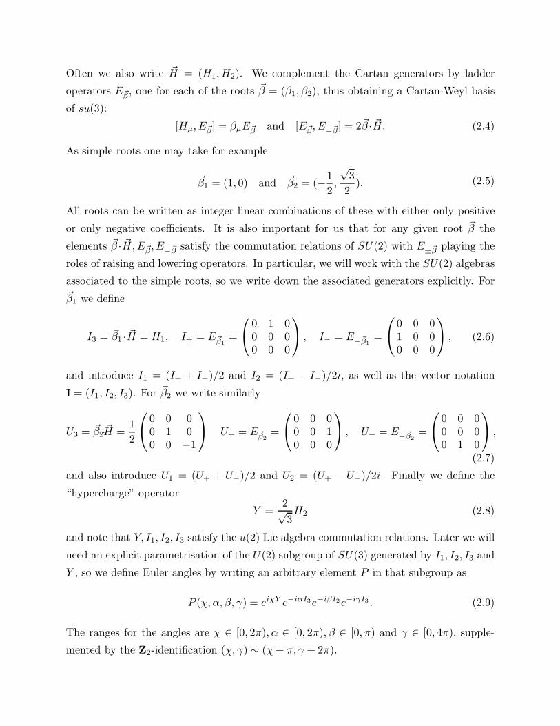
Often we also write ~H = (H1, H2). We complement the Cartan generators by ladder

operators E~β, one for each of the roots ~β = (β1, β2), thus obtaining a Cartan-Weyl basis

of su(3):

[Hµ, E~β] = βµE~β and [E~β, E−~β] = 2~β · ~H. (2.4)

As simple roots one may take for example

~β1 = (1, 0) and ~β2 = (−1

2,

√3

2). (2.5)

All roots can be written as integer linear combinations of these with either only positive

or only negative coefficients. It is also important for us that for any given root ~β the

elements ~β · ~H, E~β, E−~β satisfy the commutation relations of SU(2) with E±~β playing the

roles of raising and lowering operators. In particular, we will work with the SU(2) algebras

associated to the simple roots, so we write down the associated generators explicitly. For

~β1 we define

I3 = ~β1 · ~H = H1, I+ = E~β1

=

0 1 00 0 00 0 0

, I− = E−~β1

=

0 0 01 0 00 0 0

, (2.6)

and introduce I1 = (I+ + I−)/2 and I2 = (I+ − I−)/2i, as well as the vector notation

I = (I1, I2, I3). For ~β2 we write similarly

U3 = ~β2·~H =1

2

0 0 00 1 00 0 −1

U+ = E~β2

=

0 0 00 0 10 0 0

, U− = E−~β2

=

0 0 00 0 00 1 0

,

(2.7)

and also introduce U1 = (U+ + U−)/2 and U2 = (U+ − U−)/2i. Finally we define the

“hypercharge” operator

Y =2√3H2 (2.8)

and note that Y, I1, I2, I3 satisfy the u(2) Lie algebra commutation relations. Later we will

need an explicit parametrisation of the U(2) subgroup of SU(3) generated by I1, I2, I3 and

Y , so we define Euler angles by writing an arbitrary element P in that subgroup as

P (χ, α, β, γ) = eiχY e−iαI3e−iβI2e−iγI3 . (2.9)

The ranges for the angles are χ ∈ [0, 2π), α ∈ [0, 2π), β ∈ [0, π) and γ ∈ [0, 4π), supple-

mented by the Z2-identification (χ, γ) ∼ (χ + π, γ + 2π).

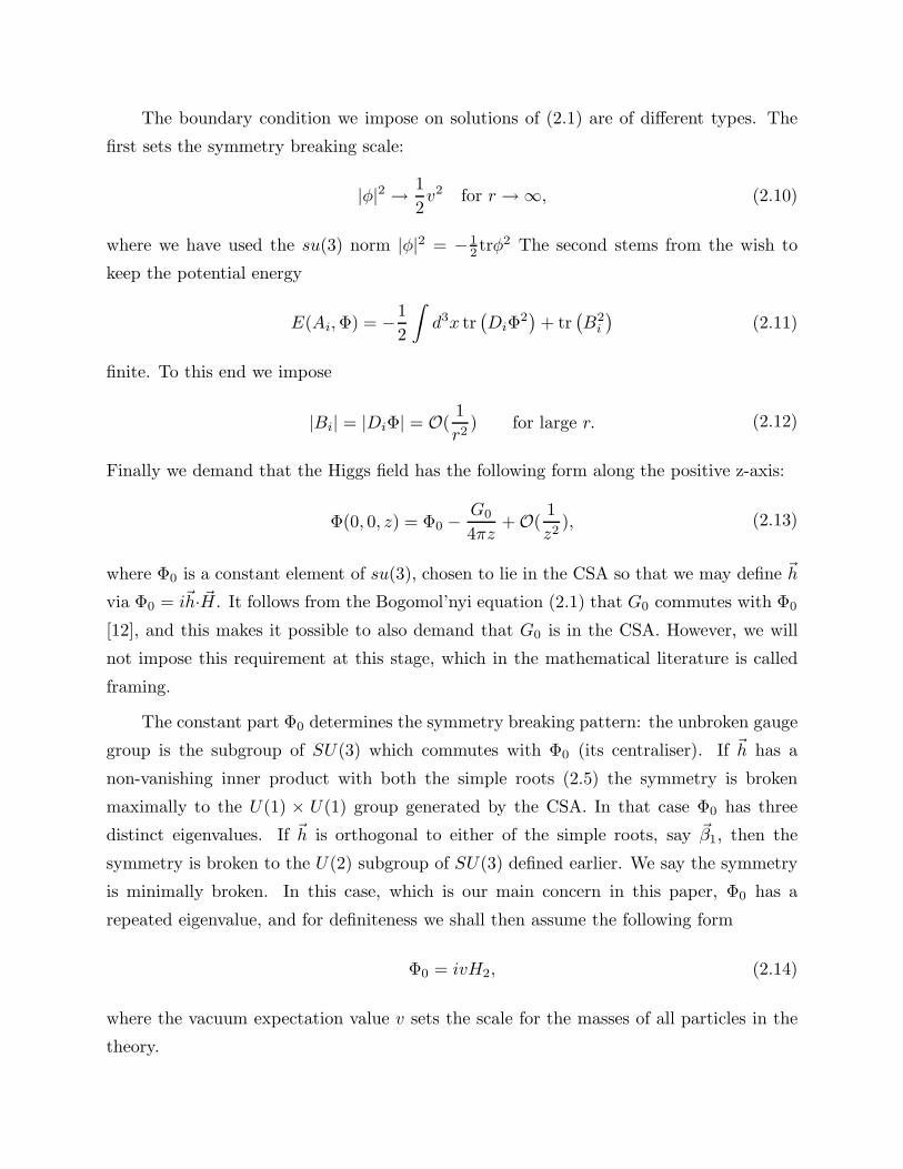
The boundary condition we impose on solutions of (2.1) are of different types. The

first sets the symmetry breaking scale:

|φ|2 → 1

2v2 for r → ∞, (2.10)

where we have used the su(3) norm |φ|2 = −12 trφ2 The second stems from the wish to

keep the potential energy

E(Ai, Φ) = −1

2

∫

d3x tr(

DiΦ2)

+ tr(

B2i

)

(2.11)

finite. To this end we impose

|Bi| = |DiΦ| = O(1

r2) for large r. (2.12)

Finally we demand that the Higgs field has the following form along the positive z-axis:

Φ(0, 0, z) = Φ0 −G0

4πz+ O(

1

z2), (2.13)

where Φ0 is a constant element of su(3), chosen to lie in the CSA so that we may define ~h

via Φ0 = i~h· ~H. It follows from the Bogomol’nyi equation (2.1) that G0 commutes with Φ0

[12], and this makes it possible to also demand that G0 is in the CSA. However, we will

not impose this requirement at this stage, which in the mathematical literature is called

framing.

The constant part Φ0 determines the symmetry breaking pattern: the unbroken gauge

group is the subgroup of SU(3) which commutes with Φ0 (its centraliser). If ~h has a

non-vanishing inner product with both the simple roots (2.5) the symmetry is broken

maximally to the U(1) × U(1) group generated by the CSA. In that case Φ0 has three

distinct eigenvalues. If ~h is orthogonal to either of the simple roots, say ~β1, then the

symmetry is broken to the U(2) subgroup of SU(3) defined earlier. We say the symmetry

is minimally broken. In this case, which is our main concern in this paper, Φ0 has a

repeated eigenvalue, and for definiteness we shall then assume the following form

Φ0 = ivH2, (2.14)

where the vacuum expectation value v sets the scale for the masses of all particles in the

theory.

The Bogomol’nyi equation relates the coefficient G0 to the coefficient of the long range

part of the magnetic field so that along the positive z-axis

B3(0, 0, z) =G0

4πz2+ O

(

1

z3

)

. (2.15)

Thus we may call G0 the vector magnetic charge. According to the generalised Dirac

quantisation condition [5], [6], the vector magnetic charge has to satisfy an integrality

condition. This is easily expressed after rotating G0 into the CSA, thus obtaining a Lie-

algebra element which we write in terms a two-component vector ~g as i~g · ~H (the vector ~g

is not, in general, uniquely defined, but this does not matter here). In the case of minimal

symmetry breaking this rotation can always be effected by the action of the unbroken gauge

group, and in the case of maximal symmetry breaking G0 is automatically in the CSA by

virtue of the vanishing of the commutator [Φ0, G0]. The generalised Dirac condition is the

requirement that ~g lies in the dual root lattice, which is spanned by the vectors

~β∗1 =

~β1

~β1 ·~β1

and ~β∗2 =

~β2

~β2 ·~β2

. (2.16)

(with our normalisation thus ~β∗1 = ~β1, ~β∗

2 = ~β2, but we keep the notational distinction for

clarity). According to the Dirac condition there exist integers m1 and m2 such that

~g =4π

e

(

m1~β∗1 + m2

~β∗2

)

. (2.17)

We will not review the derivation of the Dirac condition here but note that in the physics

literature it is usually derived without reference to the symmetry breaking pattern. As we

will see in the following section, however, the mathematical status of the two integers m1

and m2 depends on the way the gauge symmetry is broken.

3. Configuration spaces and moduli spaces

To clarify the significance of the integers m1 and m2 which appear in the Dirac con-

dition we define the (infinite dimensional) space A~h as the space or pairs (Ai, Φ) which

satisfy the boundary condition (2.13) for some fixed element Φ0 = i~h· ~H of the CSA. This

space is not acted on by the group of all static gauge transformations (which is the space

of all maps from R3 to SU(3)) but only those whose limit for z → ∞ commutes with Φ0.

In particular it is therefore acted on by the group of framed gauge transformations G0,

which is defined as

G0 ={

g : R3 → SU(3)∣

∣ limz→∞

g(0, 0, z) = id}

. (3.1)

We may thus define the framed configuration space C~h as the quotient A~h/G0. This space

is in general not connected but partitioned into disjoint sectors whose labels are called

topological charges. The topological charges are elements of the second homotopy group

of the quotient of SU(3) by the unbroken gauge group. Thus, since Π2

(

SU(3)/(U(1) ×U(1))

)

= Z2 and Π2

(

SU(3)/U(2))

= Z, the topological charges are pairs of integers in the

case of maximal symmetry breaking and a single integer in the case of minimal symmetry

breaking. It follows from the results of [13] that in the former case these are the two

integers m1 and m2 appearing in the expansion (2.17) and in the latter case this is the

integer coefficient m2 of the root ~β2 which is not orthogonal to ~h.

For minimal symmetry breaking, the vector magnetic charge G0 is in general not

invariant under the action of the unbroken U(2) gauge group and it is therefore not sur-

prising that only the invariant component tr(G0Φ0) has a topological interpretation. The

orbit of G0 under the action of U(2) is trivial only if G0 is parallel to Φ0; otherwise it is

a two-sphere in the Lie algebra of SU(3) which we call the magnetic orbit. The magnetic

orbit intersects the CSA in two points which are related by a Weyl reflection, and for any

configuration (Ai, Φ) in A~h these two points again have to satisfy the Dirac condition.

Thus, for given topological charge m2 we can label a magnetic orbit by a pair of inte-

gers [m1] = {m1, m2 − m1}. The integers {m1, m2 − m1} are called magnetic weights in

the physics literature and the pair of integers [m1] is called a holomorphic charge in the

mathematics literature. As we mentioned earlier the quantisation of the magnetic weights

has a more subtle mathematical origin than the quantisation of the topological magnetic

charges. For a precise mathematical discussion we refer the reader to [14]. The important

point is that the definition of holomorphic charges requires the connection at infinity as

well as the Higgs field. As a result it is possible for the holomorphic charges to change

in a continuous deformation of the fields which changes the connection at infinity. Unlike

topological charges, holomorphic charges may jump along a path in the configuration space

C~h.

Later we need an explicit parametrisation of the magnetic orbits. Consider the orbit

labelled by ([m1], m2). Assume without loss of generality that m1 is the larger of the two

numbers in [m1]. Then define ~g as in (2.17) and write a general point on the magnetic

orbit as

G0 = iP ~g · ~H P−1 (3.2)

with P defined as in (2.9). Computing explicitly one finds

G0 =4m2πi

e

(√3

2H2

)

+4πi

ek·I, (3.3)

where the vector k = (k1, k2, k3) has the length k = |k| = |m1 − m2

2| and the direction

given by (α, β):

k = (sin β cos α, sinβ sin α, cosβ). (3.4)

The magnetic orbits play a crucial role in the remainder of this paper and we therefore

switch to a labelling which refers directly to their geometry. Formula (3.3) shows that

we may picture the magnetic orbits as two-spheres in su(3) with quantised radii k =

0, 12 , 1, 3

2 , ... and centres on the one-dimensional lattice { 4πKie

(√3

2 H2

)

|K ∈ Z}. Thus it is

natural to introduce labels (K, k), related to ([m1], m2) via

K = m2 and k = |m1 −m2

2|. (3.5)

For the rest of the paper we will call the vector k the non-abelian magnetic charge.

To summarise: in the case of maximal symmetry breaking the configuration space C~h

is partitioned into disjoint topological sectors labelled by the pair of integers (m1, m2) but

in the case of minimal symmetry breaking the disjoint components of C~h are only labelled

by one integer K. There exists a finer subdivision according to the magnetic weight but

this is not of a topological nature. Instead it is an example of a stratification of a space,

with different strata labelled by the magnetic weights. We will describe this concretely

at the level of solutions of the Bogomol’nyi equations, or more precisely of certain sets of

solutions, called moduli spaces.

Taubes was the first to establish a rigorous existence theorem for monopole solutions

in Yang-Mills-Higgs theory for a general gauge group and general symmetry breaking pat-

tern. In [15] he proved the existence of solutions in each of the topological components

of the framed configuration space. Applied to our situation this shows that for maximal

symmetry breaking monopoles exist for all positive integers m1 and m2, but for minimal

breaking Taubes’ result only implies the existence for given positive topological charge m2

(the positivity condition results from our choice of sign in the Bogomol’nyi equations; if we

had studied the equation with the opposite sign we would obtain anti-monopole solutions

with negative topological charges). Taubes’ results say nothing about the existence of

monopoles with given magnetic weight. On the other hand, a number of explicit solutions

have been known for some time. The search for monopole solutions in Yang-Mills the-

ory (with or without Higgs field) for general gauge groups has a long history, see [16] for

the case of SU(3). It was also noticed early on that certain solutions of the Bogomol’nyi

equations of the critically coupled Yang-Mills-Higgs theory can be obtained by deforma-

tions of embedded SU(2) monopole solutions, a possibility first pointed out in [17] and

discussed further by Weinberg [12] and Ward [18]. In the latter paper it is shown that in

the minimally broken SU(3) theory solutions of arbitrary topological charge m2 can be

obtained by embeddings of SU(2) monopoles but that the magnetic weight is necessarily

[m1] = [0]; we will study these solutions in detail below. Bais and Weldon found the first

solution which cannot be constructed by embedding an SU(2) solution [19]. This solution

has topological charge m2 = 2 and magnetic weight [m1] = [1]; it is spherically symmetric

and is part of a six parameter family of axisymmetric solutions later found by Ward [20],

which we will discuss in detail later in this paper.

Monopole solutions of the same topological characteristic are conveniently grouped

together in moduli spaces. In the case of maximal symmetry breaking there is a canonical

way of defining the moduli spaces. For given Φ0 in the expansion (2.13) we fix the topo-

logical labels (m1, m2) and consider the set of all solutions of the Bogomol’nyi equation in

the corresponding component of the configuration space. In symbols:

Mmaxm1,m2

={

(Ai, Φ) ∈ A~h

∣

∣DiΦ = Bi, ~g =4π

e

(

m1~β∗1 + m2

~β∗2

)

}

/G0. (3.6)

It follows from Taubes’ existence theorem that there is a non-empty moduli space of

monopole solutions for each point in the dual root lattice shown in Fig. 1.a with positive

coordinates (m1, m2). Weinberg [12] long ago counted how many parameters’ worth of

solutions there are for each point in the dual root lattice. Translated into our language, this

determines the dimension of the moduli spaces. Observing carefully the slight differences

in conventions, Weinberg’s results translate into

dim Mmaxm1,m2

= 4(m1 + m2). (3.7)

As also pointed out by Weinberg, this dimension formula suggests that there exist

multi-monopole solutions in this theory which are made up of m1 well-separated SU(2)

monopoles embedded along the root ~β1 and m2 well-separated SU(2) monopoles embedded

along the root ~β2.

In the case of minimal symmetry breaking only the component of G0 parallel to

Φ0, labelled by the integer m2, has a topological significance. Thus one may define the

corresponding moduli spaces as

Mm2={

(Ai, Φ) ∈ A~h

∣

∣DiΦ = Bi, −2tr(G0Φ0) =4πm2i

e~β2 ·~h

}

/G0. (3.8)

However, as we learnt earlier we may classify finite-energy configurations further according

to the magnetic weight. In the mathematical literature it is customary to denote the

set of all monopoles in Mm2with magnetic weight [m1] by M[m1],m2

. Then the moduli

spaces are labelled by the same labels as the magnetic orbits, and at the risk of confusing

mathematicians who may read this paper we will use our preferred orbit labels (K, k) (3.5)

also for the moduli spaces, so we write MK,k instead of M[m1],m2. As anticipated earlier the

spaces MK,k are components of the connected space MK . In mathematical terminology one

says that the space MK is stratified with strata MK,k. It was first pointed out by Bowman

[21] that counting and interpreting the parameters of monopoles in the case of less than

maximal symmetry breaking is considerably more complicated than in the case of maximal

symmetry breaking. Murray was the first systematically to compute the dimension of the

moduli spaces of solutions in [14]. The situation is summarised in Fig. 1.b.

We can still think of each point of the dual root lattice as representing a (possibly

empty) moduli space of solutions, but we need to keep in mind that points related by

reflection at the vertical axis (which maps m1 to m2 − m1) represent the same moduli

space. The results of [14] imply that there only exist monopole solutions if the size of the

magnetic orbit is less than or equal to the (positive) topological charge K which means

that k = 0, 1, ..., K2 if K is even and k = 1

2 , 32 , ..., K

2 if K is odd. Thus solutions only occur

inside the cone (including the edge) drawn in Fig. 1.b, where we also give the dimension

which Murray computed for each of the non-empty moduli spaces. Interpreting those

dimensions physically is one of the objectives of this paper. To that end, however, we

need more explicit descriptions of the moduli spaces. We are particularly interested in the

moduli spaces on the edge of the cone and, for even K, in the centre of the cone. For

given K these are the strata of respectively smallest and largest dimensions. Hence they

are referred to respectively as the small and the large strata.

Before we give more explicit descriptions of the moduli spaces we note that the moduli

spaces we have defined are a priori only defined as sets. While there may be various

mathematically natural ways to give these sets the structure of a manifold, the physically

relevant structures are induced from the underlying field theory. In particular one would

like to induce the structure of a differentiable manifold from the field theory configuration

space and define a Riemannian metric from the field theory kinetic energy functional. This

works well for example in the case of SU(2) monopole moduli spaces [22] but is known

to be problematic for solitons in the CP1-model [23]. In the discussion of the moduli

spaces MK,k we will also encounter pathologies which are in some sense worse than in the

case of CP1 lumps. However, in order to describe these pathologies explicitly we recall

here the formal definition and general form of the metric on the moduli spaces. Consider

therefore some generic moduli space M of monopoles and suppose we have introduced

(local) coordinates X = (X1, ..., XdimM ) with components Xα, α = 1, ..., dimM on M .

Then a monopole configuration in M may be written as (Ai, Φ)(X ; r), exhibiting explicitly

the dependence on both the collective coordinate X and the spatial coordinate r. The

metric gαβ(X) is defined via the L2 norm of the infinitesimal variations (δαAi, δαΦ) which

are required to satisfy the linearised Bogomol’nyi equations and, crucially, Gauss’ law. In

the gauge A0 = 0 this reads

DiδαAi + [Φ, δαΦ] = 0. (3.9)

Then the metric can in principle be computed via

gαβ(X) = −1

2

∫

d3x tr (δαAiδβAi) + tr (δαΦδβΦ) . (3.10)

Note that by construction the Euclidean group E3 of translations and rotations in R3 and

the unbroken gauge group act on the moduli spaces we have defined and that the above

expression is formally invariant under those group actions. Thus we expect the Euclidean

group and the unbroken gauge group to act isometrically on the moduli spaces in all cases

where the above metric is well-defined.

4. Embedding SU(2) monopoles

Before we enter the general discussion of the structure of the moduli spaces we note

that a large family of SU(3) monopole solutions can be obtained by simply embedding

SU(2) monopoles. This family will be particularly important for us. The method is

simple: take a simple root which has a positive inner product with Φ0 and embed the

monopole in the associated SU(2) Lie algebra, adding a constant Lie algebra element to

satisfy the boundary condition (2.13). In discussing the explicit form of solutions we will

take the value of v (2.14) to be 12√

3in order to make contact with other explicit solutions

discussed in [24]. Thus, taking the simple root ~β2 for definiteness and referring to the

definitions (2.7) of the generators Ul, l = 1, 2, 3, we define

Φu =3∑

l=1

φlUl + diag(1,−12,−1

2)

Aui =

3∑

l=1

ailUl,

(4.1)

where (ai, φ) is a SU(2) monopole of charge K scaled so that its Higgs field tends to

diag( 32 ,−3

2) along the positive z-axis. The Higgs field of the embedded solution then has

the following expansion along the positive z-axis

Φu = Φ0 −K

ezU3 + O

(

1

z2

)

, (4.2)

showing that the embedded solution is an element of the space MK,K/2.

Note, however, that this embedding is not unique. We obtain an equally valid so-

lution after acting with the unbroken symmetry group U(2). In terms of the explicitly

parametrised element P in (2.9) we define

ΦP = PΦuP−1

APi = PAu

i P−1.(4.3)

What is the orbit under the action of P? First note that

[Y, U±] = ±U± and [I3, U±] = ∓1

2U∓ (4.4)

and hence that the configuration (4.1) is invariant under the U(1) subgroup generated by

Y + 2I3. It follows that the orbit of a given embedded configuration (Aui , Φu) under the

U(2) action is the quotient of U(2) by that U(1) group; this is a three-sphere which we

denote by S3P . This three-sphere can be coordinatised in a physically meaningful way using

the Euler angles (α, β, γ) as defined in (2.9) (the angle χ is redundant). Alternatively we

can think of elements of S3P as SU(2) matrices Q, given by

Q(α, β, γ) = e−i

2ατ3e−

i

2βτ2e−

i

2γτ3 (4.5)

This three-sphere is Hopf-fibred over the magnetic two-sphere, defined in (3.2) and we can

now write the corresponding Hopf map πkHopf , which depends on the magnitude of the

non-abelian magnetic charge:

πkHopf : Q ∈ S3

P → k ∈ S2, (4.6)

with k defined as in (3.4). The angle γ parametrises the ‘body-fixed’ U(1) rotations about

the vector k (3.3) which only change the monopole’s short-range fields. The role of this

circle is well-understood in the context of SU(2) monopoles: motion around it gives the

monopole electric charge. Thus we will call the circle parametrised by γ the electric circle.

Then we can sum up the preceding discussion by saying that the three-sphere S3P is Hopf-

fibred over the magnetic orbit S2 with fibre the electric circle.

The embedding procedure just described can be carried out for SU(2) monopoles

of arbitrary charge. The moduli space of the latter is well-understood and for magnetic

charge K it has the form

MSU2K = R3 × S1 × M0

K

ZK(4.7)

where R3 coordinatises the centre-of-mass of the charge k monopoles, the S1-factor is the

electric circle introduced at the end of the previous paragraph and M0K is the K-fold cover

of the moduli space of centred (both in R2 and S1) SU(2) monopoles of charge K. The

space MSU2K has dimension 4K. As mentioned earlier, embedding SU(2) monopoles gives

rise to SU(3) monopoles of the same topological magnetic charge and with magnetic orbit

radius K/2. In other words embeddings of SU(2) give families of SU(3) monopoles which

are elements of the small strata of the moduli space of SU(3) monopoles. In fact it is easy

to see from the Nahm data (see e.g. [21]) that all SU(3) monopoles in the small strata can

be obtained via embeddings. Thus putting together our explicit embedding prescription

with the formula (4.7) we deduce that the small strata MK,K/2 are fibred over the magnetic

orbit with the spaces MSU2K as fibres. We thus have the bijection

MK,K/2 ↔ R3 × S3P × M0

K

ZK. (4.8)

Here ZK acts on S3P by moving a fraction 2π/K round the fibre of this fibration (the

electric circle). In the fibration

MSU2K −→ MK,K/2

yπk

S2

(4.9)

the projection map πk is the forgetful map on R3 and M0K and the Hopf map (4.6) on

S3P . For later use we also introduce the notation M

K,k for the fibre (πk)−1(k). Note in

particular that the number of independent parameters in the spaces MK,K/2 is 4K + 2,

thus agreeing with the dimension found for the small strata by Murray.

We have not yet said anything about the differentiable and metric structure which

MK,K/2 inherits from the field theory kinetic energy functional via (3.10). By inspection

one checks that the moduli space metric (3.10) is well-defined on the fibres of the fibration

(4.9) and that, with that metric, the fibres are (up to an overall scaling factor of 1/3

required to agree with the conventions of [22]) isometric to the SU(2) monopole moduli

spaces. However, the mathematical structure of the magnetic orbit harbours a number of

surprises and subtleties, most of them related to physical observations made some time ago

and all of them to do with the action of the unbroken gauge group U(2). Since this group

action is of central importance for our investigation we discuss it in a separate section.

5. ‘Global Colour’ revisited

It is a standard lore in the theory of topological defects that if a defect breaks a

symmetry of the underlying theory the broken symmetry generators can be used to define

collective coordinates for the defect. However it was realised long ago by a number of

authors that this is problematic in gauge theories when the gauge symmetry gets broken

to a non-abelian group. Historically this discussion was mostly conducted in the context of

grand unified theories with gauge group SU(5) broken to SU(3)colour ×U(2)electroweak and

in that context the question of defining and dynamically exciting the collective coordinates

associated to the unbroken gauge group was put succinctly by Abouelsaood : “Are there

chromodyons ?” [25].

The answer was given partly by Abouelsaood himself and complemented by the im-

portant observation of Nelson and Manohar [26] (see also [27] ) that “Global colour is not

always defined”. Briefly, and applied to our situation, the latter authors noted that if

one writes down the Higgs field on the two-sphere at spatial infinity in any regular gauge

and attempts to define generators of a U(2) algebra which commute with the Higgs field

everywhere and vary smoothly over the two-sphere one will only succeed if the topological

magnetic charge of the configuration is even. For odd topological charge there is a topo-

logical obstruction similar to the one preventing the existence of a smooth non-vanishing

vector fields on a two-sphere; in that case it is only possible to extend a maximal torus of

U(2) over the entire two-sphere at infinity. The result of Nelson and Manohar [26] imply

that if one insists on defining a U(2) action at a fixed point (say z = +∞) in the case

of odd magnetic charge then every extension of it over the entire two-sphere at spatial

infinity will necessarily change not only the 1/r term in the asymptotic expansion of the

Higgs field but even the r0 part somewhere on the two-sphere at spatial infinity.

However, even if one allows the U(2) action to change the Higgs field (by a gauge

transformation) on the two-sphere at spatial infinity there are problems with the collective

coordinates produced by the generators which do not commute with the vector magnetic

charge G0. These were pointed out by Abouelsaood [25] who showed that infinitesimal

deformations produced by such generators do not satisfy the constraint imposed by Gauss’

law (3.9). In the following we will call collective coordinates whose infinitesimal variation

produces zero-modes which satisfy Gauss’ law and which have a finite L2-norm (so that the

corresponding components of the metric (3.10) are finite) dynamically relevant. Abouel-

saood’s result is thus that collective coordinates produced by generators of the unbroken

gauge group which do no commute with the vector magnetic charge are not dynamically

relevant.

How do these observations rhyme with our description of monopole moduli spaces in

the two preceding sections? Returning to Fig. 1.b we first note that all moduli spaces on

the vertical axis are of the form MK,0, with the topological magnetic charge K necessarily

even. Moreover the vector magnetic charge G0 is parallel to the constant part of the

Higgs field Φ0. Thus G0 is by definition invariant under the action of all generators of the

unbroken gauge group and we expect no problems in defining the action of the unbroken

gauge group on these spaces. For all the other moduli spaces, however, the magnetic charge

G0 obstructs the action of the unbroken gauge group U(2). It then follows from the results

described in the previous paragraph that only the centraliser of G0 in U(2) can have a

dynamically relevant action on these spaces.

The unbroken gauge group U(2) explicitly entered our description of the small strata

MK,K/2 and it is therefore not difficult to isolate the physically problematic coordinates

in those spaces. These are by definition coordinates associated with the generators of the

unbroken gauge group which do not commute with G0 and are therefore precisely the

coordinates on the magnetic orbit, i.e. on the base space of the fibration of the spaces

MK,K/2 in (4.9). Motion on the fibre is physically unproblematic but motion orthogonal

to the fibres is physically not permitted. The mathematical reason for this is that the

magnetic orbit inherits neither a differentiable nor a metric structure from the field theory.

On the other hand, thinking of the magnetic orbit as a two-sphere in the Lie algebra su(3)

it is natural, in view of our remarks after (3.4), to induce mathematical structure from

this embedding. In the quantum theory, to be discussed in Sect. 10, we will indeed require

some mathematical structure on the magnetic orbit, namely an integration measure (which

does not presuppose the existence of a metric structure). Thinking of the magnetic orbits

as round two-spheres of radius k (this was anticipated in defining the Hopf map πkHopf in

(4.6)) we thus define the integration measure k2 sin β dβ ∧ dα on them. Although we have

only been able to isolate the magnetic orbit explicitly as part of the moduli space in the

smallest strata we expect on physical grounds all strata MK,k with k > 0 to be fibred

over two-spheres parametrising the non-abelian magnetic charges. This conjecture does

not appear to have been considered in the mathematics literature and we are not able to

write down the projection maps for these fibrations explicitly. Nontheless we shall assume

that projection maps exist for all MK,k provided k > 0 (in this paper we will only use

them for k = K/2) and think of the base spaces of these fibrations as round two-spheres

with the integration measure given above.

The observations of Abouelsaood, Nelson and Manohar have lead most authors dis-

cussing SU(3) monopoles in the literature to discard the magnetic orbit altogether, see

[28] for a recent example. For us there are two reasons for keeping the magnetic orbit in

the discussion, and for equipping it with the measure given above. The first is that from a

certain mathematical point of view, to be described in Sect. 7, it is very natural to include

the magnetic orbit in the moduli spaces. The second and more important reason is that the

magnetic orbit plays a crucial role in the full understanding of of (classical and quantised)

dyonic excitations and of the behaviour of several interacting monopoles. In particular we

will see that is impossible to understand how two quantum states of topological charge

one monopoles combine to a quantum state of a topological charge two monopole without

taking the magnetic orbit into account. Much of the remainder of this paper is devoted to

explaining this point, but as a first step we use the next, short section to exhibit some of

the elementary questions which arise when studying classical interacting monopoles with

non-abelian magnetic charge.

6. Counting monopoles and their moduli

To begin, focus on the moduli space M1,1/2 = R3 × S3P . Physically this space sum-

marises the degrees of freedom of a single monopole in minimally broken SU(3) Yang-Mills-

Higgs theory and is therefore the basic building block for any understanding of monopole

physics in that theory. We have seen that of the monopole’s six collective coordinates only

four are dynamical: three coordinates for the monopole’s position and one for the electric

circle. Thus, dynamically a single SU(3) monopole has the same degrees of freedom as

an SU(2) monopole, but in addition it has a non-dynamical label, namely a point on a

two-sphere which specifies the direction of the vector magnetic charge in the Lie algebra

of SU(3). The crucial and interesting point is, however, that this magnetic direction and

the electric degree of freedom are not independent: the electric circle is generated by the

centraliser group of the magnetic charge. Monopoles with different magnetic directions

therefore carry charge with respect to different U(1) groups.

Now consider combining two monopoles. This can be done in two distinct ways,

corresponding to the two strata of the moduli space M2 of monopoles of topological charge

two. To obtain a configuration in the small stratum M2,1 the vector magnetic charges of

the individual monopoles have to be parallel but to obtain a configuration in the large

stratum M2,0 the vector magnetic charges should cancel and thus be anti-parallel. More

generally the restriction that the radius k of the magnetic orbit is less than or equal

to half the topological magnetic charge K, pictorially expressed in the cone structure

of Fig. 1.b, means that at least in principle it is possible to interpret configurations in

MK as being made up of K single monopoles. In particular we know already from our

discussion of the small stratum MK,K/2 that it indeed contains configurations made up of

K monopoles with all their vector magnetic charges aligned. This raises the question of

whether all strata have an asymptotic region where the moduli (and in particular their

number) can be interpreted in terms of the moduli of individual monopoles. How can

this be done? As a general principle we shall assume that in any set of well-separated

monopoles which satisfies the Dirac quantisation condition any subset must also satisfy

that condition. In particular, therefore, any pair must satisfy the Dirac condition and thus

the monopoles’ vector magnetic charges must be pairwise parallel or anti-parallel. It follows

that in a collection of K monopoles the magnetic vectors of all them necessarily lie along one

line, and only the individual positions and electric phases can be chosen independently.

One would then expect the dimension of all the strata of the moduli space MK to be

4K +2. In fact this formula is only valid for the smallest strata, where we know the above

picture to be correct. Amongst the other strata the strata of smallest magnetic weight

for given topological magnetic charge K hint at a completely different interpretation.

There the dimension is 6K, suggesting the physically puzzling interpretation of [14] that

in these moduli spaces the individual monopoles’ vector magnetic charges have somehow

escaped the constraint imposed by the Dirac condition and have become independent and

dynamical.

The next sections are devoted to a detailed investigation of these and other questions in

the case of the 12-dimensional moduli space M2,0. This is the simplest moduli space which

cannot be understood via embeddings and as a result we need to consider mathematically

more sophisticated approaches.

7. Monopoles and rational maps

The identification of monopole moduli spaces with spaces of rational maps from CP1

into certain flag manifolds goes back to conjectures of Atiyah and Murray [29] and was

first proved in the SU(2) case by Donaldson [30]. Since then generalisations of Donaldson’s

result to general gauge groups and symmetry breaking have been proved, see e.g. [31] for

recent results and further references. The results relevant for us are mostly contained in

the papers [14] and [32]. It is explained in [14] that the rational maps describing SU(3)

monopoles with minimal symmetry breaking to U(2) are based rational maps from CP1 to

CP2. Such maps are topologically classified by their degree, and this equals the topological

charge of the associated monopole. Concretely the condition that the map is based means

that the point at infinity is sent to zero, and we may write such maps as functions of one

complex variable ζ ∈ C taking values in C2 ∪ ∞. Then a rational map of degree K has

the form

R(z) =

(

p1(ζ)

q(ζ),p2(ζ)

q(ζ)

)

, (7.1)

where q is a polynomial of degree K whose leading coefficient is 1 and p1 and p2 are

polynomials of degree less than K. Writing RatK for the space of all based rational

maps from CP1 to CP2 of degree K one of the results of [14] is that there is a one-

to-one correspondence between RatK and the moduli space MK (3.8) of monopoles of

topological charge K in minimally broken SU(3) Yang-Mills-Higgs theory. There is also

a stratification of RatK which corresponds to that of the monopole moduli spaces, thus

encoding the monopoles’ magnetic weights in the rational map. A general account of how

this encoding is done can be found in [14]; in the special cases we are concerned with we

will be able to identify the magnetic weight explicitly without reference to the general

theory. One basic tool for understanding the correspondence between rational maps and

monopoles is the action of the symmetry group on the moduli spaces. In our case this

is the direct product of the Euclidean group of translations and rotations in R3 and the

unbroken gauge group U(2). This group acts naturally on the moduli space MK and hence

it has an action on RatK as well.

The U(2) action on rational maps is easy to write down. Parametrising a U(2) matrix

explicitly as eiχQ, where the SU(2)-matrix Q is parametrised as in (4.5) and the angles

(χ, α, β, γ) satisfy the Z2 condition specified after (2.9), the U(2) action on the rational

map (7.1) is(

p1

p2

)

7→ eiχQ

(

p1

p2

)

. (7.2)

The construction of rational maps from monopoles requires the choice of a preferred direc-

tion in R3 and hence breaks the symmetry of Euclidean space. We follow the conventions

of [32] where the preferred direction is the x-direction. Then a translation (x, y, z) ∈ R3

acts on a rational map as

R(ζ) 7→ e3xR(ζ − i

2(y + iz)). (7.3)

The spatial rotation group SO(3) also acts on the rational maps but this action does not

concern us here (in fact only the action of the SO(2) subgroup of rotations about the

x-axis is known explicitly).

Consider now the simplest case of a monopole of charge one. The associated rational

map has the general form

R1(ζ) = (µ1

ζ − ǫ,

µ2

ζ − ǫ). (7.4)

To understand the interpretation of the complex numbers µ1, µ2 and ǫ = ǫ1 + iǫ2 note that

his map is obtained from the standard map (0, 1/ζ) by a combined translation (7.3) and a

U(2) action if we identify

(x, y, z) =1

2(1

3ln(|µ1|2 + |µ2|2),−ǫ2, ǫ1) (7.5)

and1

√

(|µ1|2 + |µ2|2)

(

µ1

µ2

)

=

(

−ei(χ+ 1

2γ− 1

2α) sin β

ei(χ+ 1

2γ+ 1

2α) cos β

)

. (7.6)

Note in particular that the right hand side depends on (χ, γ) only in the combination

(χ + 12γ) and that we can extract the polar coordinates (α, β) for the direction of the

non-abelian magnetic charge (3.4):

e−iα tan β =µ1

µ2. (7.7)

We thus have the following interpretation of the parameters µ1, µ2 and ǫ in terms of

monopole moduli. The monopole’s position in the yz-plane is given by the complex num-

ber ǫ and the x-coordinate is determined by the length of the C2 vector (µ1, µ2)t. The

corresponding unit length vector in S3 determines the direction of the non-abelian mag-

netic charge vector via the Hopf projection

(

µ1

µ2

)

→ µ1

µ2(7.8)

and the fibre of that projection is the electric circle, parametrised by γ/2 + χ. Again we

discard the redundant angle χ.

The rational maps describing monopoles of charge two have the general form

R2(ζ) = (a + bζ

ζ2 + fζ − ǫ2,

c + dζ

ζ2 + fζ − ǫ2). (7.9)

The set of all such maps form a 12-dimensional manifold, parametrised by the complex

numbers a, b, c, d, ǫ, f . We define the strata of this manifold with the aid of the matrix

M =

(

a bc d

)

. (7.10)

The small stratum of Rat2 is defined by the condition that for all its elements the deter-

minant of M vanishes. Thus the small stratum is 10-dimensional and Murray showed [14]

that there is a one-to-one correspondence between it and the small stratum M2,1 of the

charge two SU(3) monopole moduli space. Geometrically the condition detM=0 means

that the range of the corresponding rational map lies entirely inside some CP1 ⊂ CP2.

Since CP2 is fibred over CP1 with fibre CP1 one deduces that the small stratum of Rat2 is

also fibred over CP1 with each fibre diffeomorphic to the set of rational maps CP1 → CP1

of degree two. Since the latter set is, by Donaldson’s theorem, isomorphic to the moduli

spaces of charge two SU(2) monopoles we recover the structure (4.9).

Note that the small stratum of Rat2 naturally has the structure of a complex differ-

entiable manifold whereas in the fibration (4.9) of the monopole moduli space the fibres,

but not the base space, inherit a differentiable structure from the field theory. It follows

that the bijection between the small stratum of rational maps and the small stratum of

the monopole moduli space is not a diffeomorphism.

The large stratum is defined as the set of maps in Rat2 for which the determinant of M

does not vanish. It is twelve dimensional and was shown by Dancer [32] to be diffeomorphic

to the big stratum M2,0 of the charge two monopole moduli space. Note that the rational

map description of the moduli spaces greatly clarifies the relation between the strata. We

can now see explicitly that the strata are part of the connected set Rat2 and that in a

precise sense the small stratum is the boundary of the large stratum.

Concentrating now on the large stratum M2,0 we would again like to find a physical

interpretation of the parameters occurring in (7.9). By acting on a generic rational map of

the form (7.9) with a suitable translation in the yz-plane we can set f = 0. Now consider

those maps for which |ǫ| is large. Then we may write the map (7.9) in terms of partial

fractions as

R2(ζ) =

(

µ1

ζ − ǫ+

ν1

ζ + ǫ,

µ2

ζ − ǫ+

ν2

ζ + ǫ

)

, (7.11)

with the parameters µ1, µ2, ν1 and ν2 related to a, b, c, d and ǫ via

(

µ1

µ2

)

=1

2

(

aǫ + bcǫ

+ d

)

and

(

ν1

ν2

)

=1

2

(

−aǫ + b

− cǫ

+ d

)

. (7.12)

The map (7.11) is clearly the sum of two degree one maps, and it is tempting to interpret

it as describing two monopoles located at

1

2(1

3ln 2|ǫ|(|µ1|2 + |µ2|2),−ǫ2, ǫ1) and

1

2(1

3ln 2|ǫ|(|ν1|2 + |ν2|2), ǫ2,−ǫ1) (7.13)

with internal orientation given by the vectors (µ1, µ2) and (ν1, ν2) normalised to lie on

the unit sphere S3 in C2. In particular this suggests that the individual monopoles’ non-

abelian magnetic charges have directions (α1, β1) and (α2, β2) given by

e−iα1 tanβ1 =µ1

µ2and e−iα2 tanβ2 =

ν1

ν2. (7.14)

What is remarkable here is that the magnetic orientations of the individual monopoles

appear as independent, unconstraint coordinates in the moduli space. This appears to

support Murray’s interpretation [14] that, at least in a suitable asymptotic region, M2,0

describes two monopoles with six independent dynamical degrees of freedom each. Leav-

ing aside for a moment the difficulties of talking about the individual monopole charges

in a multimonopole configuration (we return to this point in Sect. 9) it is clear that two

charge one monopoles with arbitrarily oriented vector magnetic charges would combine

to a monopole configuration whose vector magnetic charge in general violates the Dirac

condition. In the next two sections we will give a number of arguments why the interpre-

tation of the space M2,0 in terms of two monopoles with independent dynamical vector

magnetic charges is not correct. Instead the dimensionality of M2,0 can be understood by

taking into account a new dynamical coordinate which only appears when two monopoles

are combined into a monopole configuration of topological charge two.

8. Dancer’s moduli space

A detailed study of the space M2,0, including its Riemannian structure, was carried out

by Dancer in a series of papers [24] -[32] from the point of view of Nahm matrices; see also

the papers [33] and [34] with Leese, where the classical dynamics of charge two monopoles

is studied. For us the description of the isometries of M2,0 in [35] is particularly relevant.

There it is shown that M2,0 is a hyperkahler manifold whose double cover decomposes as

a direct product of hyperkahler manifolds such that one has the isometry

M2,0 = R3 × S1 × M8

Z2, (8.1)

where M8 is an eight-dimensional irreducible hyperkahler manifold. The translation group

acts only on the R3 part of the above decomposition and the central U(1) subgroup of

the unbroken gauge group U(2) acts only on the S1 factor. Thus we may think of M8 as

the space of centred SU(3) monopoles (in analogy with the space M02 in (4.7) for SU(2)

monopoles). The manifold S1 × M8 is acted on isometrically by Spin(3) × SU(2), where

Spin(3) is the double cover of the group SO(3) of spatial rotations and SU(2) is the

quotient group of the unbroken gauge group U(2) by its centre U(1). The centre of SU(2)

acts trivially but the centre of Spin(3) acts non-trivially on both M8 and on S1, the action

on the latter being rotation by π.

On the quotient M8 = M8/Z2 the Spin(3) action descends to an SO(3) action which

commutes with the SU(2) action. Thus by quotienting M8 further by the SU(2) action

one obtains a five-dimensional manifold N5 which is acted on isometrically by SO(3).

Physically this space describes monopoles with fixed centre-of-mass, quotiented by the

action of the unbroken gauge group. It turns out to have simple geometrical interpretation.

In [35] it is explained that N5 can be identified with a certain open subset of the space of

symmetric traceless 3× 3 matrices, with SO(3) acting by conjugation. We shall now show

that one can further associate a unique unoriented ellipse or line segment in R3 to a given

traceless symmetric matrix. This point of view is particularly convenient for us because it

exhibits very clearly the orbit structure of the SO(3) action.

Given a traceless symmetric matrix, diagonalise it and order the eigenvalues λ+ ≥λ0 ≥ λ−. In the generic case λ+ > λ0 > λ− call the associated eigenvectors v+, v0, v−

respectively and define an unoriented ellipse in the v+, v0 plane whose major axis is along

v+ and has length A = λ+−λ− and whose minor axis is along v0 with length B = λ0−λ−.

When λ+ > λ0 = λ− this degenerates to a line along v+ with length A = λ+ − λ− and

when λ+ = λ0 > λ− it becomes a circle orthogonal to v− with radius A = B = λ0 − λ−.

In either case the coincidence of two eigenvalues means that the matrix is invariant under

conjugation by some O(2) subgroup of SO(3) and this invariance is reflected in the axial

symmetry of the associated figure. Finally in the completely degenerate case λ+ = λ0 =

λ− = 0 the associated ellipse degenerates to a point, so both the matrix and the associated

figure are kept fixed by the SO(3) action.

When one takes the quotient of the space N5 by the SO(3) action one obtains a set

N2 which is not a manifold because the isotropy group is not the same at all points of

N5. Nonetheless the set N2 is very interesting to consider: it contains those parameters

in M2,0 which cannot accounted for by actions of the symmetry group and which therefore

may be thought of as irreducible “shape” parameters of the monopoles. In [35] it is shown

that

N2 = {(D, κ) : 0 ≤ κ ≤ 1, 0 ≤ D <2

3E(κ)}, (8.2)

where E(κ) is the elliptic integral

E(κ) =

∫ π

2

0

dθ√

1 − κ2 sin2 θ. (8.3)

In our description of N5 in terms of ellipses we also isolated shape parameters, namely

the lengths A and B of the major and minor axes. Using the explicit map between Nahm

data and traceless symmetric matrices given in [35] we can write down the relation between

these and the coordinates (D, κ) for the space N2:

A =1

2D2 and B =

1

2(1 − κ2)D2. (8.4)

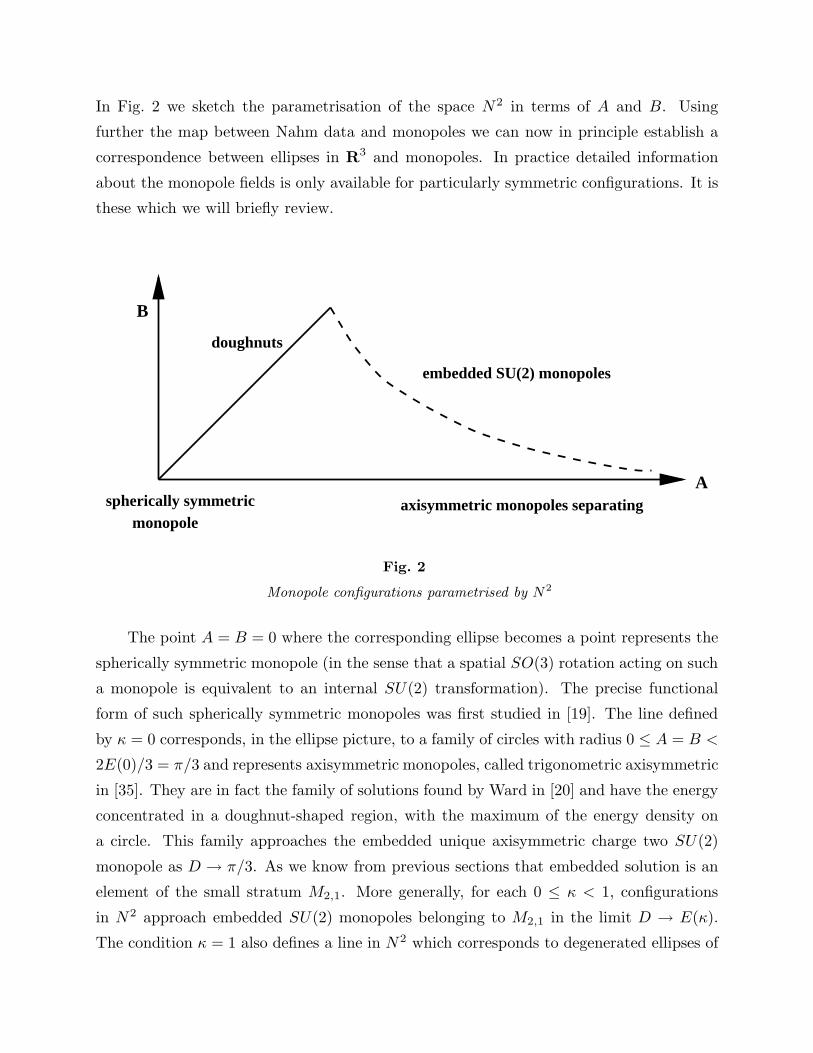
In Fig. 2 we sketch the parametrisation of the space N2 in terms of A and B. Using

further the map between Nahm data and monopoles we can now in principle establish a

correspondence between ellipses in R3 and monopoles. In practice detailed information

about the monopole fields is only available for particularly symmetric configurations. It is

these which we will briefly review.

axisymmetric monopoles separatingspherically symmetricmonopole

doughnuts

embedded SU(2) monopoles

A

B

Fig. 2

Monopole configurations parametrised by N2

The point A = B = 0 where the corresponding ellipse becomes a point represents the

spherically symmetric monopole (in the sense that a spatial SO(3) rotation acting on such

a monopole is equivalent to an internal SU(2) transformation). The precise functional

form of such spherically symmetric monopoles was first studied in [19]. The line defined

by κ = 0 corresponds, in the ellipse picture, to a family of circles with radius 0 ≤ A = B <

2E(0)/3 = π/3 and represents axisymmetric monopoles, called trigonometric axisymmetric

in [35]. They are in fact the family of solutions found by Ward in [20] and have the energy

concentrated in a doughnut-shaped region, with the maximum of the energy density on

a circle. This family approaches the embedded unique axisymmetric charge two SU(2)

monopole as D → π/3. As we know from previous sections that embedded solution is an

element of the small stratum M2,1. More generally, for each 0 ≤ κ < 1, configurations

in N2 approach embedded SU(2) monopoles belonging to M2,1 in the limit D → E(κ).

The condition κ = 1 also defines a line in N2 which corresponds to degenerated ellipses of

vanishing minor axis B and arbitrary length of the major axis A (for κ → 1 the integral

defining E(κ) diverges logarithmically). This line also represents axisymmetric monopoles,

called hyperbolic axisymmetric in [35]. The functional form and energy distribution of

these monopoles along the axis of symmetry is given in [24]. Essentially, the family of

hyperbolic axisymmetric monopoles interpolates between the spherically symmetric charge

two monopole and configurations consisting of two well-separated charge one monopoles,

with the separation approximately given by D.

Unfortunately, little is known about the fields of axisymmetric monopoles off the axis

of symmetry and about the monopoles represented by a generic point in N2 (see, however,

[33] and [34] for numerical information). The study of the axisymmetric solutions suggests

that one of the parameters in N2 should be thought of as a separation parameter, and

that, in the ellipse parametrisation, that separation is given in terms of the major axis as

D =√

2A. Then there is a complementary parameter — in the ellipse picture we think of

the length of the minor axis — which parametrises some kind of internal deformation of

the monopoles. This parameter corresponds to what in the recent literature [36] has been

called the ‘non-abelian cloud’ of the monopole. It is the goal of the next section to make

that notion more precise.

9. Monopoles and non-abelian dipoles

It is known [37] that charge two monopole solutions in spontaneously broken SU(2)

Yang-Mills-Higgs theory have no magnetic dipole moments. This is easy to understand

when the two monopoles are separated: the charges are equal, and reflection symme-

try forces dipole moments relative to the centre-of-mass to be zero. The monopoles in

minimally broken SU(3) gauge theory, however, carry vector magnetic charges and two

monopoles carrying the same topological magnetic charge may carry different non-abelian

magnetic charges. It is then natural to expect multi-monopole configurations made up of

two or more such monopoles to have non-vanishing non-abelian magnetic dipole moments.

What is more, in view of the difficulties of assigning, even in principle, individual vector

magnetic charges to monopoles in a multi-monopole configuration, dipole moments (and

possibly higher multipole moments) appear to be the only source of information about the

magnetic charges of the individual monopoles. This is the point of view we will adopt in

this section.

All the fields we study here have Higgs fields whose asymptotic expansion is consistent

with the general form

Φ(r) = Φ0(r) −G0(r)

4πr+

idaj Ia(r) rj

e2r2+ O

(

1

r3

)

(9.1)

with summation on repeated indices. Here Φ0(r) and G0(r) are the vacuum expectation

value of the Higgs field and the vector magnetic charge on the two-sphere at infinity in

some gauge (for configurations in M2,0, Φ0(r) and G0(r) are parallel everywhere), and

Ia(r), a = 1, 2, 3, are the generators of the unbroken SU(2) gauge group at a point r on

the two-sphere at infinity (since K is even there is no topological obstruction to writing

them down on the entire two-sphere at infinity). Without entering a general discussion

of multipole expansions of non-abelian gauge fields we interpret the (1/r2)-terms in the

above expansion as a dipole term. The Bogomol’nyi equation relates the (1/r2)-terms

in the Higgs fields with (1/r3)-terms in the magnetic field and we may thus consider

the coefficient matrix daj , a, j = 1, 2, 3, which transforms as a vector both under spatial

rotations and under rigid SU(2) gauge transformations, as a non-abelian magnetic dipole

moment.

We are interested in the dipole moments of monopole configurations in M2,0, but

unfortunately, explicit computations of the Higgs field for a generic configuration in this

space have only been carried by a numerical implementation of the Nahm transformation

(see [33] and [34]). The direct extraction of the dipole moments from the (explicitly known)

Nahm data seems very difficult so we restrict our discussion to configurations with extra

symmetries or to certain limits, where analytic expressions for the Higgs field have been

given in the literature. The configurations we shall discuss are essentially those which are

on or near the boundary of the set N2 depicted in Fig. 2.

We begin with hyperbolic axisymmetric monopoles. The Higgs field on the axis of

symmetry, taken to be the z-axis, was written down in [24], and extracting the (1/z2)-term

we indeed find a non-abelian component:

Φ(0, 0, z) =

(

1 − 1

2ez

)

Φ0 +iD coth 3D

2e2z2I3 + O

(

1

r3

)

. (9.2)

Since we do not know the Higgs field along any ray other than the z-axis we cannot

deduce the full tensorial structure of the dipole moment. However, we conjecture that

for a hyperbolic axisymmetric monopole configuration consisting of two monopoles well-

separated along the z-axis the dipole moment is of the form daj = dδa3δj3. From (9.2)

the coefficient d is then D coth 3D/2. For large D, D cothD ≈ D, so the dipole moment

increases linearly with separation. This is precisely the dipole moment one expects for

a configuration containing two monopoles, separated along the z-axis, with equal and

opposite non-abelian magnetic charges.

In the limit D → 0 the monopoles coalesce to the spherically symmetric solution.

Remarkably the dipole moment does not vanish in this limit. Exploiting the spherical

symmetry we can now write down the asymptotic form of the solution everywhere. In the

so-called singular gauge, where the gauge-potential has a Dirac-string singularity, it has

the form

Φ(r) =

(

1 − 1

2er

)

Φ0 +i

6e2r2I·r + O

(

1

r3

)

. (9.3)

The non-abelian dipole moment is thus seen to be of the hedgehog form dai = dδai: the Lie

algebra components of the dipole are correlated with their spatial direction in such a way

that the non-abelian dipole moment is invariant under simultaneous spatial rotations and

global SU(2) gauge rotations. In particular the dipole moment therefore does not single

out a preferred spatial direction.

Moving on to trigonometric axisymmetric monopoles we find the following expansion

along the axis of symmetry, taken to be the z-axis:

Φ(0, 0, z) = i

(

1 − 1

2ez

)

Φ0 +iD cot 3D

2e2z2I3 + O

(

1

r3

)

. (9.4)

Again we are unable to deduce the tensorial structure of the non-abelian dipole moment,

but we can determine the component d33 = cot 3D/2. Since all trigonometric axisym-

metric monopoles have their energy density concentrated in a finite region of space, their

dipole moments cannot be understood in terms of the separation and individual non-

abelian monopole charges of two single monopoles. Rather, the above expansion shows

that trigonometric axisymmetric monopoles have an intrinsic non-abelian dipole moment.

In the limit D → π/3, where the monopole configurations approach the toroidal charge

two monopole in the small stratum, the dipole strength goes to infinity, giving a very

physical interpretation of the transition between the strata: the infinite non-abelian dipole

moment combines with the (essentially abelian) vector magnetic charge of the large stra-

tum diag( 12 , 1

2 ,−1) to produce the vector magnetic charge diag(0, 1,−1) characteristic of

the small stratum.

Finally we turn to the asymptotic form of configurations near the boundary of N2

drawn as a dashed line in Fig. 2. This is studied in [38] where it is argued that for these

monopole configurations the term in the Higgs field which we call the dipole term is again

of the hedgehog form:

Φ(r) = i

(

1 − 1

2ez

)

Φ0 −iD

2(π − 3D)e2z2I·r + O

(

1

r3

)

. (9.5)

Note that near the boundary the coefficientD/2(π − 3D) is necessarily large and tends to

infinity as D → π/3.

Based on the sample of configurations studied here we propose that quite gener-

ally the parameters in N2 can be understood physically as characterising the monopoles’

non-abelian dipole moments. Configurations on the line κ = 1 which consist of two well-

separated monopoles have a purely extrinsic dipole moment. This results from the indi-

vidual monopoles’ opposite non-abelian magnetic charges and is essentially a measure of

the monopole separation. Configurations away from the line κ = 1 have dipole moments

which cannot be understood in terms of the individual magnetic charges. In particular the

fact that configurations made up of two well-separated monopoles have dipole moments of

the hedgehog type (9.5) in a certain limit shows that the fields of the two monopoles which

make up such configurations must be quite different from the fields of single monopoles

in M1,1/2. The asymptotic form (9.5) rules out the possibility, suggested by the ratio-

nal map description, that in M2,0 two well-separated monopoles have magnetic charges

with independent directions. Instead it suggests that such monopoles still have their mag-

netic charges anti-aligned, but that in addition they have individual dipole moments of

the hedgehog type. Thus we propose that the elusive cloud parameter is a measure of

the individual monopoles’ dipole strength. In the limit D → E(κ) this dipole strength

tends to infinity. The total dipole moments is then also of the hedgehog type since, for

fixed separation, the extrinsic dipole moment is negligibly small relative to the individual

hedgehog dipole moments in this limit.

Armed with a physical interpretation of the moduli in M2,0 we now turn to the quan-

tisation of monopoles. There, the conclusion that in any configuration in M2,0 which

consists of well-separated monopoles the individual monopoles’ non-abelian charges are

anti-parallel will be crucial.

10. Monopole quantisation, the dyon spectrum and the emergence of U(2)⋉R4

The quantisation of BPS monopoles in Yang-Mills-Higgs theory with gauge group

SU(2) has been studied extensively in the literature. In that case the moduli spaces are

smooth manifolds with finite metrics (and hence well-defined integration measure) and

in the standard bosonic quantisation scheme one takes the Hilbert space of states to be

the set of all square-integrable functions on the moduli space, see e.g. [39] and [40]. This

quantisation scheme needs to be amended before it can be applied to the SU(3) monopoles

studied here: the smallest strata of the moduli spaces, for example, are fibred over a two-

sphere (4.9) (the magnetic orbit) which inherits from the field theory neither a metric nor

a measure nor even a differentiable structure. The largest strata (for even K), on the other

hand, are smooth manifolds with finite metrics and the above scheme can again be applied

without difficulty. Our prescription will have to take these differences into account.

Our basic starting point is that magnetic charges label superselection sectors in quan-

tised Yang-Mills-Higgs theory. The rationale here is that magnetic charges are conserved

independently of the equations of motion and that there are no finite-action configurations

which interpolate between classical configurations with different magnetic charges. Thus

there can also be no quantum mechanical transitions between states with different magnetic

charges. This superselection rule is implicit in the standard quantisation scheme applied to

monopoles in theories with abelian unbroken gauge group. There all the magnetic charges

are topological and label disjoint moduli spaces. Superpositions between states of different

magnetic charges would correspond to linear combinations of wavefunctions on different

moduli spaces, and these are usually ruled out. In our case, the superselection sectors are

labelled by pairs (K,k) of topological and non-abelian magnetic charges. If K is even and

the non-abelian magnetic charge vanishes the corresponding sector takes the familiar form:

it is given by the Hilbert space of square-integrable functions on the moduli space MK,0

which, being the largest stratum for given K, is equipped with a smooth and finite metric.

In symbols

HK,0 = L2(MK,0). (10.1)

If k > 0 on the other hand, we label sectors also by a point k on the magnetic orbit and

define it to be the Hilbert space of square-integrable functions on the corresponding fibre

MK,k defined after (4.9) for the case k = K/2 (as also noted there, however, we expect

no principal difficulty in defining the fibres MK,k for any of the allowed pairs (K, k)).

Since these fibres are again equipped with finite and smooth metrics this definition makes

sense. However, there is another way to define the superselection sectors labelled by (K,k)

which is more useful for us. The starting point here is interpretation in the second but last

paragraph of Sect. 5 of the base spaces of the fibration MK,k → S2 as round spheres with

integration measure k2 sinβdβ ∧ dα. This allows us to define a measure on MK,k, namely

the product measure of k2 sin βdβ ∧ dα with the natural measure on the fibres (the one

coming from the metric induced by the field theory). Then it makes sense to define the

Hilbert space

HK,k = L2(MK,k). (10.2)

From this larger space we can project out the desired superselection sectors as follows.

Consider the operator

pi : HK,k → HK,k (10.3)

whose action on a function φ ∈ HK,k is

pi ◦ φ(X) = kiφ(X), (10.4)

with k = πk(X) in terms of the projection map πk defined in (4.9) for k = K/2 but

conjectured to exist for all k > 0 (in the allowed range) in Sect. 5. The simultaneous

eigenspaces HK,k of the three operators (p1, p2, p3) with eigenvalues (k1, k2, k3) contain

precisely the states with definite magnetic charge k = (k1, k2, k3) and thus correspond to

the required superselection sectors. As we shall see, this construction has a very natural

interpretation later in this paper.

Having defined the Hilbert spaces for our quantisation scheme we turn to the actions

of the various symmetry groups on these spaces. Generally speaking the symmetry group

of the theory acts on the moduli spaces, and hence also on functions on the moduli spaces,

which can therefore be organised into representations of the symmetry group. In our case

the spatial symmetry groups of translations and rotations act smoothly on the moduli

spaces, and wavefunctions can correspondingly be organised into momentum and angular

momentum eigenstates. Here we are only interested in the transformation properties of

of wavefunctions under the action of the unbroken gauge group U(2). As explained in

Sect. 5 this action is smooth and isometric only on the largest stratum of moduli spaces

for monopoles with even topological charge. On all other strata it is obstructed by the

non-abelian magnetic charge so that only the centraliser of the vector magnetic charge

acts smoothly and isometrically. Our superselection sectors reflect that difference. Thus

we expect to be able to organise the elements of HK,0 into representations of U(2) while

elements of HK,k should be organised into representation of the centraliser of k. In the

former case we may therefore denote dyonic quantum states by |K, 0; N, j, m〉, where K

is the topological magnetic charge, N is an integer which specifies the representation of

the U(1) transformation generated by Y (2.8) and the half-integers j ∈ {0, 12 , 1, 3

2 ...},m ∈ {−j,−j + 1, ..., j − 1, j} specify a state |jm〉 in an SU(2) representation; the three

numbers (Njm) then specify a state in an U(2) representation, and we need to impose the

Z2 condition that N is odd if j is a half-odd integer and N is even if j is an integer. The

other sort of dyonic states can be written as |K,k; N, s〉, where K and N have the same

meaning as before, k is the non-abelian magnetic charge defined in (3.4), and s is a single

half-integer which specifies the representation of the U(1) subgroup of SU(2) which leaves

k fixed. Again we have the condition that N is odd if s is half-odd and N is even if s is

integer.

We now show how these states are realised as wavefunction on the moduli spaces.

Since all the essential features of the scheme we are going to propose show up already for

monopoles of topological charge K ≤ 2, we will restrict attention to the corresponding

moduli spaces in the following. Thus we will be able to draw on the explicit description of

those spaces in the previous sections.

Again we begin with a single monopole and the moduli space M1,1/2 = R3 × S3P . As

explained in sects. 5 and 6, this space is fibred over the magnetic orbit S2. A point k

on the magnetic orbit specifies the non-abelian magnetic charge and obstructs the U(2)

action: only the centraliser acts smoothly. For an explicit description of quantum states

of a single monopole it is convenient to write a generic SU(2) matrix in terms of Pauli

matrices and Euler angles (α, β, γ) as in (4.5) and to introduce Wigner functions Djms(Q) =

e−imαdjms(β)e−isγ on SU(2) following the conventions of [41]. The functions Dj

ms, j ∈{0, 1

2, 1, 3

2, ...}, m, s ∈ {−j,−j+1, ..., j−1, j} form a basis for the Hilbert space L2(SU(2)),

and one can moreover (formally) expand the δ-function on SU(2) in terms of them. We

write the δ-function peaked at the point Q and with argument Q′ as δE(Q′Q−1), where

E is the identity element. Then, putting primes on the Euler angles for Q′ we have the

formula

δE(Q′Q−1) = δ(α′ − α)δ(cos β′ − cos β)δ(γ′ − γ) (10.5)

and the expansion

δE(Q′Q−1) =∑

j=0, 12,1...

j∑

m=−j

j∑

s=−j

2j + 1

16π2D∗j

ms(Q′)Dj

ms(Q). (10.6)

Quantum states for a single monopole are of the form |1,k; N, s〉, where |k| = 1/2

and we have the constraint N + 2s = 0 as a consequence of the monopole’s invariance

under the generator Y + 2I3. Since the point k on the magnetic orbit is obtained from

a general point Q on SU(2) via the Hopf projection we have the explicit parametrisation

in terms of Euler angles k = (sinβ cos α, sin β sin α, cosβ). Furthermore we can give an

explicit realisation of the states of a single monopole in terms of Euler angles:

〈χ′, α′, β′, γ′|1,k; N, s〉 = eiNχ′

δ(α′ − α)δ(cosβ′ − cos β)eisγ′

, (10.7)

where the condition N = −2s ensures that the right hand side only depends on 2χ′ − γ′.

Then, using the above completeness relation (10.6) we also deduce

〈χ′, α′, β′, γ′|1,k; N, s〉 = eiNχ′∑

j≥|s|

m=j∑

m=−j

2j + 1

4πDj∗

ms(Q′)e−imαdj

ms(β). (10.8)

Turning next to two monopoles, we have to distinguish the two strata. Quantum

states on the small stratum are again much like the quantum states of a single monopole.

They are of the form |2,k; N, s〉, where now |k| = 1 and we again have the constraint

N + 2s = 0. These states can be realised as wavefunctions on the moduli space M2,1.

The most general wavefunction will also depend on the centre-of-mass position and on the

relative coordinates summarised in the Atiyah-Hitchin manifold M02 , but here we are only

interested in the dependence on S3P . This dependence is just like for the quantum states

of a single monopole:

〈χ′, α′, β′, γ′|2,k; N, s〉 = eiNχ′∑

j≥|s|

m=j∑

m=−j

2j + 1

4πDj∗

ms(Q′)e−imαdj

ms(β), (10.9)

where now |k| = 1. There may appear to be an inconsistency in our notation at this stage,

in that the magnetic labels appear on the right hand side of (10.8) and (10.9), but not on

the left. However, the rationale for our notation will soon become clear.

The large stratum M2,0 is smooth with a finite metric and, like in the case of SU(2)

monopoles, quantum states can be realised as smooth wavefunctions on the moduli space.

The magnetic orbit is trivial in this case, so all coordinates should be treated on the same

footing. The most general wavefunction depends on the U(2) Euler angles (χ, α, β, γ), on

the centre-of-mass position, on spatial Euler angles and on the shape parameters (A, B).

A detailed investigation of the quantum mechanics on M2,0 would be a very interesting

but also very challenging project. Here we are merely interested in the transformation

properties of the wavefunction under the unbroken gauge group U(2) so we focus again

on the wavefunction’s dependence on the corresponding coordinates. Making use of the

fact that, for any fixed s in the allowed range, both the Wigner functions Djms and their

complex-conjugates Dj∗ms, m ∈ {−j,−j + 1, ..., j − 1, j} span the spin j representation of

SU(2), we may choose a value for s and then represent dyonic quantum states as follows:

〈χ′, α′, β′, γ′|2, 0; N, j, m〉s =

√2j + 1

4πeiNχ′

Dj∗ms(Q

′). (10.10)

Different values for s lead to equally valid realisations of the state |2, 0; N, j, m〉, but we

introduce the suffix s here because we shall see further below that this half-integer also

has a physical interpretation.

Having represented dyonic quantum states with topological magnetic charges one and

two as wavefunctions on the relevant moduli spaces we are in a position to address one

of the key concerns of this paper: what is the relationship between the tensor product of

two quantum states of a single monopole and a quantum state of a topological charge two

monopole? The answer to this question can in principle be deduced from a knowledge of the

algebraic object whose representations are being studied. In our case we do not yet know

the relevant algebraic object. It is clearly not simply the unbroken gauge group U(2) since

the quantum states we have studied carry in general only a representation of a subgroup

of it, namely the centraliser of the non-abelian magnetic charge. The algebraic object

we seek should incorporate the subtle interplay between magnetic and electric properties

which we have seen in the dyonic states discussed so far. We will now argue that for

dyonic states in the present theory the relevant algebraic object is the semi-direct product

U(2) ⋉ R4. Denoting the generators of U(2) again by I1, I2, I3 and Y and calling the

translation generators p1, p2, p3 and P the Lie algebra of U(2) ⋉ R4 has the following

commutation relations

[Ia, Ib] = iǫabcIc

[pa, pb] = 0

[Ia, pb] = iǫabcpc

[Y, P ] = [Y, Ia] = [Y, pa] = [P, Ia] = [P, pa] = 0, for a = 1, 2, 3.

(10.11)

To test this proposal we first show that the representations contain precisely the dyonic

states discussed above and then show that the Clebsch-Gordan coefficients of U(2) ⋉ R4

are consistent with the representation of states as wavefunctions on moduli spaces.

The semi-direct product U(2) ⋉ R4 is an example of a regular semi-direct product

and therefore its representation theory is most effectively dealt with via the method of

induced representations [42]. For a general regular semi-direct product S = H ⋉ N , where

N is an abelian, normal subgroup of S, the construction of an irreducible representation

begins with the classification of all H orbits O in N , the set of characters of N . Each orbit

has a characteristic centraliser group C (the centraliser group of any point on it) and a

unitary irreducible representations (UIR) can then be induced from the group C ⋉N . The

representation space VO,ρ of an UIR of S constructed in this way is then labelled by the

orbit O and a UIR ρ of the stability group C:

VO,ρ ={

φ : H → Vρ

∣

∣φ(QX) =ρ(X−1)φ(Q) ∀Q ∈ H, X ∈ C

and

∫

H/C

||φ||2(z)dµ(z) < ∞}

,(10.12)

where Vρ is the carrier space of the representation ρ, ||·|| is the norm induced by the inner

product in Vρ and dµ is an invariant measure on the coset H/C ∼= O. One can show that

all UIR’s of S can be obtained in this way.

Applying this theory to our case we first note an obvious simplification. Since U(2) =(

U(1) × SU(2))

/Z2 we have a corresponding direct product decomposition U(2) ⋉ R4 =(

(U(1)⋉R)× (SU(2)⋉R3))

/Z2. The interesting part of the representation theory comes

from the non-abelian part SU(2) ⋉ R3, which happens to be the double cover of the

Euclidean group in three dimensions and whose representation theory is particularly well

documented in the literature. In this case the set of characters R3

of the translation

group R3 is isomorphic to R3 and can physically be thought of as momentum space, with

elements denoted by k. The SU(2) orbits in R3

are spheres with radius k > 0 or simply a

point. In the former case the centraliser group is U(1) and in the latter the entire group

SU(2). By the general theory we thus obtain two sorts of UIR’s of SU(2) ⋉ R3. If k > 0

the carrier spaces are infinite dimensional and labelled by the orbit size k > 0 and a

half-integer s specifying a U(1) representation. They may be realised as follows

Vk,s ={

φ : SU(2) → C∣

∣φ(Qe−i

2ξτ3) =eisξφ(Q)

and

∫

S2

|φ|2(α, β) sinβ dβdα < ∞}

.(10.13)

The action of an element (A, a) ∈ SU(2) ⋉ R3 on this Hilbert space is given by

((A, a) ◦ φ)(Q) = eia·kφ(A−1Q), (10.14)

where k is obtained from Q via the Hopf projection (4.6) i.e. k = πkHopf(Q). Having earlier

introduced Wigner functions SU(2) as a basis of L2(SU(2)) one checks that for fixed s the

functions Dj∗ms, j ∈ {|s|, |s|+ 1, ...},m ∈ {−j,−j + 1, ..., j − 1, j} form a basis of Vk,s.

In the case k = 0 the general prescription of induced representation theory starts from

a standard (2j+1)-dimensional representation of SU(2) with carrier space C2j+1 on which

Q ∈ SU(2) is represented by the matrix Djms(Q), s, m ∈ {−j,−j +1, ..., j−1, j}, and leads

to the Hilbert space

V0,j ={

φ : SU(2) → C2j+1∣

∣φs(QQ′) =

j∑

t=−j

Djst(Q

′−1)φt(Q)}

, (10.15)

where φs denotes the s-th component of φ. The action of (A, a) ∈ SU(2) ⋉ R3 reduces to

an SU(2) action:

((A, a) ◦ φ)(Q) = φ(A−1Q), (10.16)

Again it is straightforward to write down a basis. Since the right action of SU(2) on itself

is transitive the value of any element φ ∈ V0,j is determined by its value at the identity.

Since the possible values at the identity are parametrised by C2j+1 we see explicitly that

V0,j is (2j + 1)-dimensional. We further define a basis {φ(m)}m=−j,−j+1,...,j−1,j consisting

of those elements of V0,j which reduce to the canonical basis of C2j+1 at the identity:

φ(m)s (E) = δms. It then follows that

φ(m)s (Q) = Dj

sm(Q−1) = Dj∗ms(Q). (10.17)

By now it will be apparent to the reader that Wigner functions are omnipresent in the

representation theory of the Euclidean group, where they play a number of different roles.

Here we find them as the components of C2j+1-valued basis functions of V0,j . Note in

particular that under the SU(2) transformation (10.16) the components of the vector-

valued functions φ(m) do not get mixed:

(A ◦ φ(m))s(Q) = φ(m)s (A−1Q) =

j∑

l=−j

Djlm(A)φ(l)

s (Q). (10.18)

Thus, for any fixed s in the allowed range the component functions φ(m)s (Q) = Dj∗

ms(Q),

m ∈ {−j,−j+1, ..., j−1, j} span an equally valid carrier space of the spin j representation

of SU(2).

In order to complete our account of the representation theory of U(2)⋉R4, we need to

combine the above representations with representations of U(1) ⋉ R. Thinking about the

latter from the point of view of induced representation may seem unnecessarily complicated

but it is useful for a unified view. The U(1) action on R (by conjugation) leaves every

point fixed, so all orbits are trivial and consist of a real number K ∈ R. The centraliser

is always the whole of U(1), so centraliser representations are labelled by a single integer

N . All UIR’s are one-dimensional and given by

vK,N ={

φ : U(1) → C∣

∣φ(χ + ξ) = eiNξφ(χ) ∀χ, ξ ∈ [0, 2π)}

. (10.19)

Clearly this is just the one-dimensional space spanned by the function φN (χ) = eiNχ. The

action of an element (ξ, a) ∈ U(1) ⋉ R on this function is

(ξ, a) ◦ φN (χ) = eiKaφN (χ − ξ). (10.20)

The representations of SU(2)⋉R3 and of U(1)⋉R can now be combined to representations

of U(2) ⋉ R4 by taking tensor products of individual representations, but respecting the

Z2 conditions on N and j or N and s outlined earlier. Thus carrier spaces of UIR’s of

U(2) ⋉ R4 are of the form

VK,k;N,s = vK,N ⊗ Vk,s (10.21)

with k > 0 and N + 2s even, or

VK,0;N,j = vK,N ⊗ V0,j (10.22)

with N+2j even. We will use the unifying notation VK,k;N,n for these representations, with

n standing for the U(1) representation label s ∈ 12Z if k > 0 for the SU(2) representation

label j ∈ {0, 12, 1, ...} if k = 0.

We now come to the promised identification of dyonic quantum states of SU(3)

monopoles with elements of U(2) ⋉ R4 representations, partly already anticipated by our

notation. Our proposal is to identify the magnetic charges with the eigenvalues of the

translation generators P and p1, p2, p3 of U(2)⋉R4, and the electric charges with the rep-

resentations of the centraliser subgroups of U(2). More precisely we identify the topological

magnetic charge with the representation label K and the magnitude of the non-abelian

magnetic charge with the representation label k. Then we associate the dyonic states

discussed earlier with the representation spaces of U(2) ⋉ R4 as follows. For k > 0, the

realisation of states |K,k; N, s〉 as wavefunctions on the moduli space (10.8) and (10.9)

shows that they can be written as infinite sums of elements of VK,k;N,s. In fact these sums

do not converge, but since these states are eigenstates of the translation generators p1, p2

and p3, their non-normalisability is the familiar property of of momentum eigenstates in

quantum mechanics on R3. Keeping that proviso in mind we write

|K,k; N, s〉 ∈ VK,k;N,s. (10.23)

The dyonic states with k = 0 can be interpreted as elements of the representation space

VK,0;N,j if we identify the label s in the realisation of |K, 0; N, j, m〉 (10.10) with the s-th

component of elements of VK,0;N,j:

〈χ′, α′, β′, γ′|K, 0; N, j, m〉s = eiNχ′

φ(m)s (Q′). (10.24)

With this identification we can then also write

|K, 0; N, j, m〉 ∈ VK,0;N,j. (10.25)

One immediate question which arises after this identification concerns the quantisation

of the magnetic charges. The eigenvalues of the translation generators are not naturally

quantised, so by interpreting quantum states of magnetic monopoles as eigenstates of the

translation operators we select a subset of translation eigenstates by hand, namely those

with integer eigenvalues K and half-integer values for the magnitude of k. We return to the

group theoretical interpretation of this quantisation in the final section of this paper. Now

we impose the quantisation and press on, turning to the computation of the combination

rules of dyonic states. These can now be found using the Clebsch-Gordan coefficients

of U(2) ⋉ R4. The interesting part of this is again the (double cover) of the Euclidean

group, whose Clebsch-Gordan coefficients can be found in the literature see e.g. [43]. Their

calculation is lengthy (remarkably we could not find them in any group theory textbook)

because of the subtleties of combining representations with different orbits and centraliser

representations. To give a flavour of the subject we note the following Clebsch-Gordan

series for the tensor product of two representations. Multiplying two representation with

non-vanishing orbit sizes k1 and k2 one finds:

Vk1,s1⊗ Vk2,s2

=

∫ k1+k2

|k1−k2|dk

∞∑

t=−∞Vk,s1+s2+t, (10.26)

where k = 0 is allowed on the right hand side; in that case the sum over s1 + s2 + t is a

sum over SU(2) representations and should be restricted to positive integers. Physically

one may think of this formula in terms of combining plane waves with wave vectors k1 and

k2 and helicities s1 and s2. If the magnitudes of the wave vectors are fixed to be k1 and k2

the combined plane wave may have wave vectors with length k varying between |k1 − k2|and k1 + k2 and a helicity which is integer or half-odd integer depending on the values of

s1 and s2 but otherwise arbitrary. If k1 = k > 0 and k2 = 0, the tensor product splits into

a finite sum of irreducible representations:

Vk,s ⊗ V0,j =

j⊕

n=−j

Vk,s+n. (10.27)

Finally the case k1 = k2 = 0 reproduces the familiar SU(2) Clebsch-Gordan series:

V0,j1 ⊗ V0,j2 =

j1+j2⊕

j=|j1−j2|V0,j . (10.28)

We are actually interested in more detailed information, namely the Clebsch-Gordan

coefficients which specify the relation between states. On the other hand we only need to

consider very special states, namely those singled out by the Dirac quantisation condition

on the magnetic charge. This condition should be imposed on both the states to be

multiplied and on the resulting product state, and this drastically reduces the number

of tensor products we need to consider. Here we have only treated quantum states of

monopoles of topological magnetic charge 1 and 2, but we propose as a general requirement

that the non-abelian magnetic charges k1 and k2 of two states to be multiplied must be

parallel or anti-parallel. It is clear that then all states obtained as the tensor of two states

which individually satisfy the Dirac condition will also satisfy that condition.

Starting with quantum states of topological charge one monopoles |1,k1; N1, s1〉 and

|1,k2; N2, s2〉 for example, where k1 = k2 = 1/2 and N1 + 2s1 = N2 + 2s2 = 0, we may

thus only combine them if either k1 = k2 or k1 = −k2. In the former case the tensor

product is

|1,k; N1, s1〉 ⊗ |1,k; N2, s2〉 = δ2(0)|2, 2k; N1 + N2, s1 + s2〉, (10.29)

where the infinite factor δ2(0) arises because we are working with non-normalisable states.

The equations (10.29) is essentially the combination rule for monopoles with abelian mag-

netic charges: the direction of k does not come into play in any interesting way. This

agrees with the fact that the quantum states in (10.29) can all be realised as wavefunc-

tions on the smallest stratum of the relevant moduli space and that these strata are fibred

of the magnetic orbit, with fibres being isomorphic to SU(2) monopole moduli spaces. The

combination rule (10.29) is the combination rule of SU(2) monopoles in a fixed fibre. The

possibility of anti-parallel non-abelian magnetic charges is much more interesting. Now

the tensor product is

|1,k; N1, s1〉 ⊗ |1,−k; N2, s2〉

= δ2(0)∞∑

j=|s1−s2|

j∑

m=−j

√

2j + 1 djm(s1−s2)

(β)e−imα |2, 0; N1 + N2, j, m〉s1−s2,

(10.30)

where (α, β) are again the angles determining the direction of k as in (3.4). Here the

representation theory of U(2) ⋉ R4 has entered in a non-trivial way and has solved one of

the main puzzles of non-abelian dyon physics, namely how to combine two dyons carrying

non-abelian magnetic charge and U(1) × U(1) electric charge into a dyon carrying only

topological magnetic charge and a U(2) representation. Particularly we now also see how

to decompose a quantum state |2, 0; N, j, m〉 of a charge two monopole in terms of tensor

product states of charge one monopoles

δ2(0)|2, 0; N, j, m〉s =∫

sin βdβdα

√2j + 1

4πdj∗

ms(β)eimα |1,k; N1, s1〉 ⊗ |1,−k; N2, s2〉,(10.31)

with the condition N1 + N2 = N and s1 − s2 = s. Note that all magnetic directions are

needed on the right hand side. If we had only considered single monopole states with a

particular magnetic directions we would not be able to make sense of general charge two

monopole quantum states in terms of tensor product states of charge one monopoles.

We have not discussed monopoles of topological charge three here, but for complete-

ness we also write down the rule for combining a quantum state of a charge one monopole

with a quantum state of a charge two monopole in the large stratum. The former carries

U(1) electric charge and latter U(2) electric charge, but within the representation theory

of U(2) ⋉ R4 there is no problem in combining such states. The answer is

|1,k; N1, s1〉 ⊗ |2, 0; N2, j, m〉s2=

√2j + 1

4πeimαdj∗

ms2|3,k; N1 + N2, s1 + s2〉, (10.32)

with k of length 1/2 and direction given by (α, β).

Having demonstrated the use of interpreting dyonic quantum states of SU(3)

monopoles as elements of U(2) ⋉ R4 representations we end this section by highlight-

ing two restrictions which are dictated by the physics of monopoles but which are not

naturally part of U(2) ⋉ R4 representation theory. The first restriction is the superselec-

tion rule that states with different (topological or non-abelian) magnetic charge may not

be superimposed. The second is a consequence of the Dirac condition and is the restriction

on which states may be multiplied in tensor products.

11. BPS quantum states and S-duality

Maximally broken N = 4 supersymmetric Yang-Mills theory is widely believed to

enjoy exact invariance under S-duality transformations. In general but precise terms this

statement means the following. For a given gauge group G and symmetry breaking to a

group H consider the two real parameters which uniquely characterise the action of N = 4

supersymmetric Yang-Mills theory, namely the coupling constant e and the θ-angle. Then

construct the complex number τ = θ/2π + 4πi/e2 in the upper half plane. An S-duality

transformation is a modular transformation on τ

τ → qτ − r

−pτ + s, (11.1)

where M =

(

q −r−p s

)

∈ SL(2,Z), together with a suitable SL(2,Z) action on the BPS

states of the quantum theory (to be defined presently). If H is a maximal torus of G,

the BPS states are dyonic states characterised by R =rank(H)=rank(G) pairs of integers

(ml, nl), l = 1, ..., R, giving the magnetic and electric charges respectively [4]. Under

S-duality these states transform as

(ml, nl) → (ml, nl)M−1 (11.2)

for all l = 1, ..., R. In particular the electric-magnetic duality operation originally consid-

ered by Montonen and Olive [10] is given by the matrix

M =

(

0 1−1 0

)

, (11.3)

which exchanges strong with weak coupling and electric with magnetic charges.

Little is known about duality in theories with non-abelian unbroken gauge symmetry.

There exists a conjecture, due to Goddard, Nuyts and Olive [6] according to which Yang-

Mills-Higgs theory with gauge group G broken to H has a dual description at strong

coupling in terms of weakly coupled Yang-Mills-Higgs theory with a dual gauge group G

broken to H. The GNO conjecture interprets the non-abelian monopole charges, after

rotation into the Cartan subalgebra, as labels of irreducible interpretations of the dual

group H. The true invariance group of Yang-Mills-Higgs theory with unbroken gauge group

H would, according to the GNO conjecture, be the product H × H of an “electric” and a

“magnetic” version of the unbroken gauge group. In particular the GNO conjecture would

imply that dyonic states fall into representations of that product group. However, here

we have seen that dyonic quantum states of monopoles in minimally broken SU(3) Yang-

Mills-Higgs theory have correlated magnetic and electric properties, with the magnetic

orbit determining the part of the unbroken gauge group with respect to which the dyons

carry electric charge. This correlation is not accounted for by the representation theory

of the GNO group U(2) × U(2), but, as we have seen, it is captured perfectly by the

representation theory of the semi-direct product U(2) ⋉ R4. In particular the Clebsch-

Gordan coefficients of U(2) ⋉ R4 lead to combination rules for dyonic states which are

consistent with their realisation as wavefunctions on the moduli spaces.

The goal of this section is to look at the implications of our insights into the dyonic

spectrum for S-duality in Yang-Mills theory with non-abelian unbroken gauge symmetry.

We will consider transformation rules for dyonic states which generalise the abelian rules

(11.2) to the non-abelian case with minimal modifications. In particular we thus consider

transformation rules which map the dyonic states of minimally broken SU(3) Yang-Mills-

Higgs theory into dyonic states of the same theory with dual coupling (11.1). We are

aware that this may well be too restrictive. In particular we feel that one needs a better

understanding of duality in the massless sector of the N = 4 supersymmetric version of

the theory before one can gain a full understanding of duality. However, the massless

sector has essentially the same particle contents as unbroken N = 4 supersymmetric U(2)

Yang-Mills theory, whose dual formulation is not known [44]. We do not attempt to solve

this problem here and focus on the massive particles instead. As we shall see, there is a

natural SL(2,Z)-duality action on the massive dyonic states, whose study is instructive.

We are particularly interested in BPS states, which are (in general) dyonic states in some

representation VK,k;N,n of U(2) ⋉ R4 whose energy equals the BPS bound

EBPS = ve|N + τK|. (11.4)

where v is the magnitude (2.14) of the vacuum expectation value of the Higgs field.

The starting point for the transformation rule we want to consider is the observation

of the previous section that dyonic quantum states fit into certain representations of U(2)⋉

R4. This generalises in the obvious way to dyonic states in Yang-Mills-Higgs theory with

general unbroken gauge group H: these states fall into certain representations of H ⋉ RD

(D =dim(H). Thus (as we shall explain in more detail in [9]) they are labelled by R

quantised orbit parameters and by R labels specifying the representation of the centraliser

group associated to the orbit (which always contains a maximal torus and therefore has

the same rank as H). This is also (trivially) true in the maximal symmetry breaking

case, where the orbits are always just points in a R-dimensional lattice and the centraliser

is always the whole of H. In that case, as we saw above, electric-magnetic duality acts

by exchanging orbit labels with centraliser representation labels. In this formulation the

electric-magnetic duality transformation rule naturally generalises to the situation where

H is non-abelian. Again we focus on the case G = SU(3) and H = U(2).

In that case we have seen that magnetic orbits are labelled by the pair (K, k), with

K ∈ Z and 0 ≤ k ≤ K/2 integer or half-odd integer depending on whether K is even

or odd, which may be summarised as the requirement that K + 2k is even. Centraliser

representations are labelled by the pair (N, n), where N ∈ Z specifies a U(1) representation

and n defines a centraliser representation as specified after (10.22). Again we have a Z2

condition relating N and n, namely that N + 2n is even. The S-duality action we want to

consider involves the SL(2,Z) action on the τ -parameter (11.1) together with the following

action on the representation labels:

(K, N) → (K, N)M−1

(k, n) → (k, n)M−1.(11.5)

Recall that in the abelian case, where all representations are one-dimensional, there is

either no or a unique BPS state (or, more precisely, a unique short N = 4 supermultiplet)

in the representation labelled by (ml, nl). Thus there is no difference between an SL(2,Z)

action on representations and an SL(2,Z) action on states. In the non-abelian case, how-

ever, we have to decide whether we consider the action of S-duality on the entire carrier

space of representations or just on certain states in those spaces. A moment’s thought

shows that one cannot expect the carrier spaces of the representations related by (11.5) to

be “physically equivalent”: for example the purely electric representation V0,0;1,1/2 is two-

dimensional whereas the purely magnetic representation V1,1/2;0,0 is infinite-dimensional.

On may hope that the BPS condition will select the same number of states in all represen-

tations related by (11.5), but this is not case as we shall see. We postpone a full discussion

of this puzzle until the end of this section. Here we note that the alternative route, that

of considering the action of S-duality on individual states in the spaces VK,k;N,n, can be

implemented quite easily. The idea is to select a unique state in each carrier space VK,k;N,n

by a “natural” condition (which necessarily breaks the U(2) ⋉R4 invariance of the carrier

spaces maximally). One can do this, for example, by picking a unit vector k and in each

VK,k;N,n select that state which is the eigenstate of the SU(2) generator k·I with maximal

(or minimal) eigenvalue. If k = 0 this condition selects the state in the spin j representation

of SU(2) with spin j along the k axis; if k > 0 it selects the state |K, kk; N, n〉 (provided

n ≥ 0). While this condition may appear ad hoc we will see at the end of this section that

it has played an important role in earlier discussions of electric-magnetic duality.

Consider now the SL(2,Z) orbit of the massive W -bosons of the theory on which

previous discussions of electric-magnetic duality have traditionally focused. The massive

W -bosons form a doublet under SU(2) and carry one unit of U(1) charge, so they belong

to the representation (K, k) = (0, 0) and (N, n) = (1, 1/2). Under the SL(2,Z) transfor-

mation (11.5) this is mapped to

(K, k) = p(1, 12 ) (N, n) = q(1, 1

2 ), (11.6)

for relatively prime integers p and q. These states carry magnetic charge, and at weak

coupling should be visible semi-classically. More precisely, since k = K/2, they should

emerge as dyonic states in the smallest strata of the moduli spaces we have described.

Since these moduli spaces consist of embedded SU(2) monopoles we can hope to deduce

the prediction of S-duality in this case from the S-duality properties of the SU(2) theory.

This is in fact what we will do, but since our computation needs to be carried out in the

N = 4 supersymmetric version of the purely bosonic theory we have described so far,

we first need to explain how N = 4 supersymmetry is implemented in our quantisation

scheme.

The general procedure for implementing supersymmetry in the collective coordinate

or moduli space quantisation of monopole dynamics is explained in [45] in the context of

SU(2) monopoles. For N = 4 supersymmetry this procedure leads to the Hilbert space of

states being the space of all square-integrable real differential forms on the moduli space

and the Hamiltonian being the covariant Laplacian. An important consistency requirement

is that the metric on the moduli space is hyperkahler. The arguments given in [45] apply

without essential changes to the largest strata of the moduli spaces we have described,

i.e. those labelled by K even and k = 0. These spaces have dimension 6K (which is thus

divisible by four) and are equipped with smooth hyperkahler metrics. All the other strata,

however, have dimensions which are even but not divisible by four, indicating clearly that

the standard procedure needs to be amended. In fact the required changes follow naturally

from the magnetic superselection rules introduced in the previous section. Namely, the

Hilbert spaces HK,k introduced after (10.4) can be extended to accommodate N = 4

supersymmetry in the standard fashion. Their elements are functions on the fibres MK,k

of the fibration (4.9) and these spaces do have dimensions which are multiples of four. In

the case k = K/2 they are actually isomorphic to SU(2) monopole moduli spaces and thus

in particular equipped with hyperkahler metrics. It has not been shown rigorously that

for k < K/2 these spaces also have smooth hyperkahler metrics, but non-rigorous physical

arguments suggest that they do. Here we are in any case mainly interested in the case

k = K/2, so we fix this condition from now on.

Then we define the space H∗K,k of square-integrable real differential forms on MK,k.

The quantum Hamiltonian is the Laplacian on MK,k, which equals, up to scaling, the

Laplacian on the SU(2) monopole moduli space MSU(2)K . The eigenstates of that Hamilto-

nian which saturate the BPS bound, however, were conjectured by Sen [2] to exist, and be

unique, for all (K, N) = (p, q) relatively prime integers. There is now much support for the

validity of the Sen conjecture [2], [3], and assuming it we deduce the existence of a unique

dyonic BPS state for each value of the non-abelian magnetic charge k in the U(2) ⋉ R4

representation VK,K/2;N,N/2 with (K, N) = (p, q) relatively prime integers. Thus we indeed

find the BPS states on the SL(2,Z) orbit of the massive W -boson states, but we encounter

the puzzle anticipated earlier in this section: whereas the massive W -bosons fill the two-

dimensional representation V0,0;1,1/2, the dyonic BPS states fill the infinite-dimensional

representations VK,K/2;N,N/2.

In earlier discussion of duality e.g. in [6] this “dimensionality puzzle” is not seen

because only vector magnetic charges on the orbit of a given vector magnetic charge un-

der the action of the Weyl group of the unbroken gauge group are considered. It follows

from general group theory that the number of points on the Weyl orbit of the vector

magnetic charge of a topological charge one monopole is equal to the dimension of the

fundamental representation of the unbroken gauge group. Thus, with this counting proce-

dure the number of massive W -boson states agrees with the number of topological charge

one monopoles. This observation is in fact a key ingredient in the formulation of the GNO

conjecture in [6]. Here, however, we have seen that the full magnetic orbit is essential

for understanding dyonic states and their interaction, and that any restriction to a subset

of the orbit is artificial and will miss some of the physics of dyons. From our point of

view the restriction to Weyl orbits is equivalent to choosing a direction k and restricting

attention to states which are eigenstates of the operator k · I introduced earlier in this

section. Thus GNO duality in the theory considered here would, in our language, amount

to choosing k = (0, 0, 1) and selecting the eigenstates of I3 with maximal and minimal

eigenvalues. This condition selects the usual basis of massive W -boson states in the purely

electric sector V0,0;1,1/2 while in the magnetic sector V1,1/2;0,0 it picks out two monopoles

with magnetic charges on the same Weyl orbit (the Weyl group of U(2) is the permutation

group S2 of two elements and acts on the magnetic orbits we have defined by sending a

point to its antipodal point). Such a choice can be made, but it is ad hoc and breaks the

symmetry of the theory in an artificial way.

We end this section with two comments. The first concerns the place of Weyl orbits

in our description of dyons. Although we do not select any particular Weyl orbit in our

scheme, Weyl orbits do play an important role. Dyonic states with non-abelian magnetic

charges in the same Weyl orbit have parallel or anti-parallel non-abelian magnetic charges

and are thus precisely those states in VK,k;N,s which may be multiplied in a tensor product.

Thus, although the representation space VK,k;N,s is infinite-dimensional for k > 0, a given

state can interact consistently with at most two other states in the same representation.

This is intriguingly reminiscent of the role Weyl orbits play in the physics of classical

non-abelian electric charges. In [46] points on Weyl orbits were shown to correspond

one-to-one to the relative orientations which two non-abelian electric point charges may

have if the non-abelian electric field they produce is to be static. These observations are

not a sufficient reason to assign any dimension other than infinity to the carrier spaces

VK,k;N,s (k > 0) but they do show that counting degrees of freedom for particles carrying

non-abelian charges is a subtle business.

The second comment concerns the paper [11]. In that paper, a regularisation proce-

dure was used to make motion on (in our language) the magnetic orbit dynamically possible

and a supersymmetric quantisation scheme was adopted which allowed forms on the mag-

netic orbit as physical states. In that scheme computing the degeneracies of magnetic

states is equivalent to counting harmonic forms on the magnetic orbit, i.e. to computing

its Euler characteristic. However, the Euler characteristic of the coset spaces considered

in [11] is equal to the number of points in the orbit under the Weyl group of the unbroken

gauge group of any point in the coset. We relegate a discussion and proof (which is a

simple application of Morse theory) of this statement for general gauge groups to [9], but

in the theory considered in this paper the validity is easily demonstrated. Here the relevant

coset is the magnetic orbit whose Euler characteristic is two if k > 0 and one if k = 0.

Similarly the orbits of the Weyl group acting on the magnetic orbit have order two if k > 0

and order one if k = 0. Thus, the counting procedure for magnetic states described in [11]

also boils down to determining the order of Weyl orbits.

12. Discussion and outlook

The mathematical structure of the monopole moduli spaces described in this paper

singles out certain coordinates, called magnetic orbits here, and only allows smooth iso-

metric actions of a subgroup of the unbroken gauge group, namely the centraliser group

associated to the orbit. As a result magnetic orbits and electric centraliser representations

turn out to be the natural labels of dyonic quantum states in minimally broken SU(3)

Yang-Mills-Higgs theory. Noting that orbits and centraliser representations are also the

attributes of representations of the semi-direct product U(2) ⋉ R4 we have proposed to

interpret dyonic states as elements of such representations. It is worth stressing again that

this group is not a symmetry of the classical theory and that in particular the magnetic

part R4 does not act on either the classical configuration space or the moduli spaces.

Nonetheless we have seen that the wavefunctions on the moduli space are acted upon by

the full group U(2) ⋉ R4. Thus, although one usually thinks of the electric excitations

as quantum effects and the magnetic properties as classical, we find that in our scheme

the magnetic properties are also encoded in quantum wavefunctions. Furthermore, the

interpretation of dyonic states as elements of representations of U(2) ⋉ R4 leads to com-

bination rules of dyonic states which are consistent with the realisation of dyonic states as

wavefunctions on the appropriate moduli spaces.

However, while thinking of dyonic states as elements of U(2) ⋉ R4 representations

turns out to be very fruitful, it also raises a number of questions, the most important of

of which concerns the quantisation of the magnetic orbit sizes: from the point of view of

U(2)⋉R4 representations this is an artificial condition, while in monopole physics it is one

of the most basic facts. Ideally we would like the algebraic object which classifies dyonic

quantum states to incorporate quantised magnetic orbit sizes (or equivalently the Dirac

quantisation condition) as a basic ingredient. It remains a challenge to find that algebraic

object, which we expect to be closely related to semi-direct product groups.

A second question concerns the S-duality properties of the dyonic spectrum. We

have seen that it is possible to define an SL(2,Z)-action on the dyonic states of the

theory, with the electric-magnetic duality operation exchanging labels of the magnetic

orbits with labels of the centraliser representations. With this definition the basic massive

W -boson states are seen to be part of an SL(2,Z)-orbit whose other elements are dyonic

BPS states which can be found semi-classically as quantum states on the smallest strata

of monopole moduli spaces. However, in interpreting these BPS states as elements of

U(2)⋉R4 representations we are forced to conclude that S-duality relates states belonging

to U(2) ⋉ R4 representations of different dimensions. We expect that a solution of this

“dimensionality puzzle” will require a deeper understanding of S-duality in supersymmetric

Yang-Mills theory with non-abelian unbroken gauge symmetry.

To end, we want to stress a link to physics in (2+1) dimensions. In [47] it was shown

that dyonic quantum states of vortices in (2+1)-dimensional gauge theories with discrete

unbroken gauge groups are labelled by magnetic fluxes together with a centraliser repre-

sentation of the unbroken gauge group. There the relevant algebraic object whose repre-

sentations classify the dyonic states is the so-called quantum double D(H) of the unbroken

gauge group H, which by definition is the tensor product of the algebra of functions on the

group with the group algebra. Dyons in two spatial dimensions have distance-independent

topological interactions (Aharanov-Bohm scattering, flux metamorphosis) and remarkably

these can be deduced from the algebraic structure of D(H). More recently quantum

doubles have also been constructed for continuous groups, such as SU(2) [48] and were

found to have a number of structural similarities to semi-direct product groups of the

type discussed here, with the function algebra in the quantum double being related to the

translation part of the semi-direct product groups. The intriguing relation between these

two algebraic objects deserves to be studied further. The important lesson one learns from

studying quantum states of both vortices with non-abelian flux and monopoles with non-

abelian magnetic charge is that consistent algebraic classifications of these states require

that one treats magnetic and electric properties as interdependent aspects of one algebraic

object.

Acknowledgements

We are grateful to Robbert Dijkgraaf, Erwyn van der Meer, Nathalie Muller, Herman

Verlinde and Mark de Wild Propitius for discussions. BJS also thanks Conor Houghton,

Nick Dorey, Patrick Irwin, Stuart Jarvis, Klaas Landsman, Nick Manton, Jae-Suk Park

and especially Andrew Dancer for discussions, is grateful to the Isaac Newton Institute for

hospitality during a two-week visit in January 1997 and acknowledges financial support

through a Pionier Fund of the Nederlandse Organisatie voor Wetenschappelijk Onderzoek

(NWO).

References

[1] G. ’t Hooft, “Magnetic monopoles in unified gauge theories”, Nucl. Phys. B 79 (1974)

276 ;

A.M. Polyakov, “Particle spectrum in quantum field theory” JETP Letters 20 (1974)

194.

[2] A. Sen, “Dyon-monopole bound states, self-dual harmonic forms on the multi-

monopole moduli space, and SL(2,Z) invariance in string theory”, Phys. Lett. B

329 (1994) 217.

[3] G. Segal and A. Selby, “Cohomology of spaces of monopoles”, Commun. Math. Phys.

177 (1996) 775.

[4] J. Gauntlett and D. Lowe, “Dyons and S-duality in N=4 supersymmetric gauge the-

ory”, Nucl. Phys.B472 (1996) 194 ;

K. Lee, E.J. Weinberg and P. Yi, “Electromagnetic duality and SU(3) monopoles”

Phys. Lett.B 376 (1996) 97 ;

G.W. Gibbons, “The Sen conjecture for fundamental monopoles of distinct type”,

Phys. Lett. B 382 (1996) 53.

[5] F. Englert and P. Windey, “Quantization condition for ’t Hooft monopoles in compact

simple Lie groups”, Phys. Rev. D 14 (1976) 2728.

[6] P. Goddard, J. Nuyts and D. Olive, “Gauge theories and magnetic charge”, Nucl.

Phys. B 125 (1977) 1.

[7] E. Corrigan and D. Olive, “Colour and magnetic monopoles”, Nucl. Phys. B 110

(1976) 237.

[8] R.A. Brandt and F. Neri, “Stability analysis for singular non-abelian magnetic

monopoles”, Nucl. Phys. B 161 (1979) 253.

[9] F.A. Bais and B.J. Schroers, “Non-abelian dyons and S-duality”, in preparation.

[10] C. Montonen and D.Olive, “Magnetic monopoles as gauge particles ?”, Phys. Lett. B

72 (1977) 117.

[11] N. Dorey, C. Fraser, T.J. Hollowood and M.A.C. Kneip, “Non-abelian duality in N=4

supersymmetric gauge theories”, hep-th/9512116 ;

“S-duality in N=4 supersymmetric gauge theories with arbitrary gauge group”,Phys.

Lett.B 383 (1996) 422.

[12] E.J. Weinberg, “Fundamental monopoles and multimonopole solutions for arbitrary

simple gauge groups”, Nucl. Phys. B 167 (1980) 500.

[13] C.H. Taubes, “Surface integrals and monopole charges in non-abelian gauge theories”,

Commun. Math. Phys. 81 (1981) 299.

[14] M. Murray, “Stratifying monopoles and rational maps”, Commun. Math. Phys. 125

(1989) 661.

[15] C.H. Taubes, “The existence of multi-monopole solutions to the non-abelian Yang-

Mills-Higgs equations and arbitrary gauge groups”, Commun. Math. Phys. 80, (1981)

343.

[16] A. Chakrabarti, “On classical solutions of SU(3) gauge field equations”, Ann. Inst.

H. Poincare 23 (1975) 235 ;

W.J. Marciano and Heinz Pagels, “Classical SU(3) gauge theory and magnetic

monopoles”, Phys. Rev. D 12, (1975) 1093 ;

Z. Horvath and L. Palla, “Dyons in classical SU(3) gauge theory and a new topolog-

ically conserved quantity”, Phys. Rev. D 14 (1976) 1711 ;

E. Corrigan, D.I. Olive, D.B. Fairlie and J. Nuyts, “Magnetic monopoles in SU(3)

gauge theory”, Nucl. Phys. B 106 (1976) 475

[17] F.A. Bais, “Charge-monopole duality in spontaneously broken gauge theories”, Phys.

Rev. D 18 (1978) 1206.

[18] R.S. Ward, “Deformations of the embedding of the SU(2) monopole solution in

SU(3)”, Commun. Math. Phys. 86 (1982) 437.

[19] F.A. Bais and H.A. Weldon, “Exact Monopole Solutions in SU(n) gauge theory” Phys.

Rev. Lett. 41 (1978) 601 ;

D. Wilkinson and F.A. Bais, “Exact SU(N) monopole solutions with spherical sym-

metry’ , Phys. Rev. D 19 (1979) 2410.

[20] R.S. Ward, “Magnetic monopoles with gauge group SU(3) broken to U(2)”, Phys.

Lett. B 107 (1981) 281.

[21] M.C. Bowman, “Parameter counting for self-dual monopoles”, Phys. Rev. D 32 (1985)

1569.

[22] M.F. Atiyah and N. Hitchin, The geometry and dynamics of magnetic monopoles,

Princeton University Press, New Jersey 1988.

[23] R.S. Ward, “Lumps in the CP1-model in (2+1) dimensions”, Phys. Lett. B 158

(1985) 424.

[24] A.S. Dancer, “Nahm data and SU(3) monopoles”, Nonlinearity 5 (1992) 1355.

[25] A. Abouelsaood, “Are there chromodyons?”, Nucl. Phys. B 226 (1983) 309.

[26] P.N. Nelson and A. Manohar, “Global colour is not always defined”, Phys. Rev. Lett.

50 (1983) 943.

[27] A. Balachandran et al., “Monopole topology and the problem of color”, Phys. Rev.

Lett 50 (1983) 1553.

[28] M. Alvarez, “Physical states of dyons”, SWAT-97-156, hep-th/9707117.

[29] M.F. Atiyah, “Instantons in two and four dimensions”, Commun. Math. Phys. 93

(1984) 437 ;

M.F. Atiyah, “Magnetic monopoles in hyperbolic space”, In “Vector bundles on Al-

gebraic Varieties”, Oxford University Press, 1987.

[30] S.K. Donaldson, “Nahm’s equation and the classification of monopoles”, Commun.

Math. Phys. 96 (1984) 387.

[31] S. Jarvis, “Euclidean monopoles and rational maps ”, Oxford University preprint 1997,

submitted to Proc. London Math. Soc. .

[32] A.S. Dancer, “A family of Hyperkahler Manifolds”, Quart. Jour. Math. 45 (1994) 463.

[33] A.S. Dancer and R.A. Leese, “Dynamics of SU(3) monopoles”, Proc. Roy. Soc. Lond.

A440 (1993) 421.

[34] A.S. Dancer and R.A. Leese, “A numerical study of SU(3) charge-two monopoles with

minimal symmetry breaking”, Phys. Lett. B 390 (1997) 252.

[35] A.S. Dancer, “Nahm’s equation and Hyperkahler Geometry”, Commun. Math. Phys.

158 (1993) 545.

[36] K. Lee, E.J. Weinberg and P. Yi, “Massive and massless monopoles with nonabelian

magnetic charges”,Phys. Rev. D 54 (1996) 6351.

[37] N.S. Manton and T.M. Samols “Radiation from monopole scattering”, Phys.Lett. B

215 (1988) 559.

[38] P. Irwin, “SU(3) monopoles and their fields”, DAMTP preprint 97-33, hep-

th/9704153.

[39] G.W. Gibbons and N.S. Manton, “Classical and Quantum Dynamics of BPS

monopoles”, Nucl. Phys. B 274 (1986) 183.

[40] B.J. Schroers, “Quantum scattering of BPS monopoles at low energy”, Nucl. Phys. B

367 (1991) 177.

[41] D.A. Varshalovich, A.N. Moskalev and V.K. Khersonskii, Quantum Theory of Angular

Momentum, World Scientific, Singapore 1988.

[42] A.O. Barut and R. Raczka, Theory of group representations and applications, PWN,

Warszawa 1977.

[43] J.S. Rno, “Clebsch-Gordan coefficients and special functions related to the Euclidean

group in three-space”, J. Math. Phys. 15 (1974) 2042 ;

N.P. Landsman, “Non-shell unstable particles in thermal field theory”, Ann. Phys.

186 (1988) 141.

[44] Y. Lozano, “Duality and canonical transformations”, Talk at Argonne Duality Insti-

tute, June 1996, hep-th/9610024.

[45] J. P. Gauntlett, “Low-energy dynamics of N=2 supersymmetric monopoles”, Nucl.

Phys. B 411 (1994) 443 ;

J. D. Blum, “Supersymmetric quantum mechanics of monopoles in N=4 Yang-Mills

Theory”, Phys. Lett. B 333 (1994) 92.

[46] E. Corrigan, “Static non-abelian forces and the permutation group”, Phys. Lett. B

82 (1979) 407.

[47] F.A. Bais, P. van Driel and M. de Wild Propitius, “Quantum symmetries in discrete

gauge theories”, Phys. Lett. B 280 (1992) 63 ;

M. de Wild Propitius and F.A. Bais, “Discrete gauge theories”, Proc. CRM-CAP Sum-

mer School “Particles and fields ’94”, Banff, Springer Verlag (1996), hep-th/9511201.

[48] T.H. Koornwinder and N.M. Muller, “The quantum double of a (locally) compact

group”, J. of Lie Theory 7 (1997) 101; “The quantum double of SU(2)”, in preparation;

F.A. Bais, T.H. Koornwinder and N.M. Muller “Decomposition of tensor products of

the quantum double of a compact group”, in preparation.