Meson properties from Lattice QCD

John N. HedditchSupervisors: D. B. Leinweber and A. G. Williams

Centre for the Subatomic Structure of MatterUniversity of Adelaide

Adelaide2006

This thesis is dedicated to Kati - you are proof the universe is a wonderful place.

Abstract

Quantum Chromo-Dynamics (QCD) is the part of the Standard Model which describesthe interaction of the strong nuclear force with matter. QCDis asymptotically free, so athigh energies perturbation expansions in the coupling can be used to calculate expectationvalues. Away from this limit, however, perturbation expansions in the coupling do notconverge.

Lattice QCD (LQCD) is a non-perturbative approach to calculations in QCD. LQCDfirst performs a Wick rotationt → −itE , and then discretises spacetime into a regularlattice with some lattice spacinga. QCD is then expressed in terms of parallel transportoperators of the gauge field between grid points, and fermionfields which are definedat the grid points. Operators are evaluated in terms of thesequantities, and the latticespacing is then taken to zero to recover continuum values.

We perform computer simulations of Lattice QCD in order to extract a variety ofmeson observables. In particular, we perform a comprehensive survey of the light andstrange meson octets, obtain for the first time exotic meson results consistent with exper-iment, calculate the charge form-factor of the light and strange pseudoscalar mesons, anddetermine (for the first time in Lattice QCD) all three form-factors of the vector meson.

Statement of Originality

This work contains no material which has been accepted for the award of any otherdegree or diploma in any university or other tertiary institution and, to the best of myknowledge and belief, contains no material previously published or written by anotherperson, except where due reference has been made in the text.

I give consent to this copy of my thesis, when deposited in theUniversity Library,being available for loan and photocopying, and further consent to it’s reproduction as amusical or theatrical work.

John N. Hedditch

Acknowledgements

• Thank you first of all to Derek Leinweber and Tony Williams, mysupervisors, fortheir tremendous patience, wisdom, and calm, all of which are attributes I woulddearly love to posess myself.

• Big Ups to Ben Lasscock for his organisational genius and committment to being ateam-player(TM).

• My Hat Off and great thanks to Sara Boffa and Sharon Johnson who have saved mefrom ruin many a time.

• Three Cheers to James Zanotti, Ross Young, Waseem Kamleh, Alex Kalloniatis,Tony Thomas, Marco Ghiotti and Marco Bartolozzi, Mariusz Hoppe, and all thoseothers who have made working at the CSSM one of the most enjoyable times of mylife.

• Thank you to Ramona Adorjan and Grant Ward for computing support, and senseof humour under pressure.

• The Australian Partnership for Advanced Computing, the South Australian Partner-ship for Advanced Computing, and the National Facility for Lattice Gauge Theoryprovided the computational muscle for this project, which would have been quiteimpossible otherwise.

• Finally, a big thankyou to all of my family, and Kati’s family, for their support inthis endeavour. It’s been a wild ride.

ix

Contents

Abstract v

Statement of Originality vii

Acknowledgements viii

1 Introduction 11.1 Quantum Chromodynamics . . . . . . . . . . . . . . . . . . . . . . . . . 1

2 Lattice QCD 42.1 Introduction . . . . . . . . . . . . . . . . . . . . . . . . . . . . . . . . . 42.2 Discrete symmetries . . . . . . . . . . . . . . . . . . . . . . . . . . . . . 5

2.2.1 Symmetries of Correlation functions . . . . . . . . . . . . . .. . 52.2.2 Generalisation . . . . . . . . . . . . . . . . . . . . . . . . . . . 72.2.3 Proofs . . . . . . . . . . . . . . . . . . . . . . . . . . . . . . . . 8

3 Mesons from LQCD 93.1 Introduction . . . . . . . . . . . . . . . . . . . . . . . . . . . . . . . . . 93.2 Meson correlation functions at the hadronic level . . . . .. . . . . . . . 9

3.2.1 Lorentz Scalar fields . . . . . . . . . . . . . . . . . . . . . . . . 93.2.2 Lorentz Vector fields . . . . . . . . . . . . . . . . . . . . . . . . 10

3.3 Analysis . . . . . . . . . . . . . . . . . . . . . . . . . . . . . . . . . . 113.4 Meson correlation functions at quark level . . . . . . . . . . .. . . . . 13

3.4.1 Mesonic operators from the naive quark model . . . . . . . .. . 133.5 Hybrid Mesons . . . . . . . . . . . . . . . . . . . . . . . . . . . . . . . 14

3.5.1 Introduction . . . . . . . . . . . . . . . . . . . . . . . . . . . . . 143.5.2 Method . . . . . . . . . . . . . . . . . . . . . . . . . . . . . . 153.5.3 Results . . . . . . . . . . . . . . . . . . . . . . . . . . . . . . . 173.5.4 Summary . . . . . . . . . . . . . . . . . . . . . . . . . . . . . . 25

3.6 Exotic Mesons . . . . . . . . . . . . . . . . . . . . . . . . . . . . . . . 303.6.1 Introduction . . . . . . . . . . . . . . . . . . . . . . . . . . . . 303.6.2 Physical Predictions . . . . . . . . . . . . . . . . . . . . . . . . 323.6.3 Summary . . . . . . . . . . . . . . . . . . . . . . . . . . . . . 36

xi

4 Source dependence of Hybrid and Exotic signal 414.1 Introduction . . . . . . . . . . . . . . . . . . . . . . . . . . . . . . . . . 414.2 Method . . . . . . . . . . . . . . . . . . . . . . . . . . . . . . . . . . . 434.3 Results . . . . . . . . . . . . . . . . . . . . . . . . . . . . . . . . . . . . 43

4.3.1 Hybrid Pion . . . . . . . . . . . . . . . . . . . . . . . . . . . . . 434.3.2 Exotic . . . . . . . . . . . . . . . . . . . . . . . . . . . . . . . . 53

4.4 Discussion and Summary . . . . . . . . . . . . . . . . . . . . . . . . . . 58

5 Meson form factors 595.1 Introduction . . . . . . . . . . . . . . . . . . . . . . . . . . . . . . . . . 595.2 Three-point function with current insertion . . . . . . . . .. . . . . . . . 59

5.2.1 π-meson case . . . . . . . . . . . . . . . . . . . . . . . . . . . . 615.2.2 Spin-1 case . . . . . . . . . . . . . . . . . . . . . . . . . . . . . 615.2.3 Extracting static quantities . . . . . . . . . . . . . . . . . . . .. 64

5.3 Method . . . . . . . . . . . . . . . . . . . . . . . . . . . . . . . . . . . 665.4 Results . . . . . . . . . . . . . . . . . . . . . . . . . . . . . . . . . . . . 675.5 Conclusions . . . . . . . . . . . . . . . . . . . . . . . . . . . . . . . . . 88

6 Conclusions 89

A Data pertaining to the calculation of meson effective masses 94

B Obtaining the form of 〈r2〉 104

C Source dependence results for the SU(3)β = 4.60, 203 × 40 lattice 105

D Quark-level calculations 110D.1 Two-point function . . . . . . . . . . . . . . . . . . . . . . . . . . . . . 110D.2 Electromagnetic current insertion . . . . . . . . . . . . . . . . .. . . . . 111

E REDUCE script for calculating ratios of three to two-point functions 112

F Data pertaining to the calculation of meson form-factors 114

G Papers by the author 121

xii

List of Figures

1.1 Quark-flow diagrams for three-point and two-point mesonvertices. . . . . 11.2 The scalar meson octet and singletη′. Image courtesy of WikiImages . . . 2

3.1 Author’s sketch of a quark-model meson vs a hybrid meson .. . . . . . . 143.2 Effective mass for standard pseudovector interpolating field, for equal

(left) and unequal (right) quark-masses. Results are shownfor all eightmasses. . . . . . . . . . . . . . . . . . . . . . . . . . . . . . . . . . . . 17

3.3 Effective mass for axial-vector pion interpolating field, for equal (left) andunequal (right) quark-masses. Results are shown for all eight masses. . . 17

3.4 Effective mass for the hybrid pion interpolating fieldiqaγjBabj q

b, for equal(left) and unequal (right) quark-masses. Results are shownfor all eightmasses. . . . . . . . . . . . . . . . . . . . . . . . . . . . . . . . . . . . 18

3.5 Effective mass for the hybrid pion interpolating fieldiqaγjγ4Babj q

b, forequal (left) and unequal (right) quark-masses. Results areshown for alleight masses. . . . . . . . . . . . . . . . . . . . . . . . . . . . . . . . . 18

3.6 Ground (triangles) and excited state (circles) masses for the pion, ex-tracted using a3× 3 variational process using the first three pion interpo-lating fields. Signal is only obtained for the heaviest 3 quark masses. . . 19

3.7 Thea0 scalar meson correlation function vs. time. . . . . . . . . . . . . 203.8 ρ-meson effective mass derived from standardqγjq interpolator. Re-

sults are shown for both equal (left) and unequal (right) quark-antiquarkmasses. Results for every second quark mass are depicted. . .. . . . . . 22

3.9 ρ-meson (left) andK∗ (right) effective mass plots derived from interpola-tor qγjγ4q. Every second quark mass is depicted. . . . . . . . . . . . . . 22

3.10 Vector meson effective mass from hybrid interpolatorqaEabj q

b. Everysecond quark mass is depicted, and results are depicted for both ρ (left)andK∗ (right) mesons. . . . . . . . . . . . . . . . . . . . . . . . . . . . 22

3.11 Vector meson effective mass from hybrid interpolatoriqaγ5Babj q

b. Everysecond quark mass is depicted, and results are depicted for both ρ (left)andK∗ (right) mesons. . . . . . . . . . . . . . . . . . . . . . . . . . . . 23

3.12 Vector meson effective mass from hybrid interpolatoriqaγ4γ5Babj q

b. Ev-ery second quark mass is depicted, and results are depicted for bothρ(left) andK∗ (right) mesons. . . . . . . . . . . . . . . . . . . . . . . . . 23

xiii

3.13 Effective mass plots fora1 axial-vector meson interpolator. Results areshown for light (left) and strange-light (right) quark-masses. . . . . . . . 24

3.14 b1 axial-vector meson effective mass. Results are shown for both light(left) and strange-light (right) quark masses. . . . . . . . . . .. . . . . . 24

3.15 Summary of results for pion interpolating fields.m2π, derived from the

standard pion interpolator, provides a measure of the inputquark mass. . 253.16 Summary of results for K interpolating fields.m2

π, derived from the stan-dard pion interpolator, provides a measure of the input quark mass. . . . 26

3.17 Summary of results forρ-meson interpolating fields.m2π, derived from

the standard pion interpolator, provides a measure of the input quark mass. 273.18 Summary of results forK∗-meson interpolating fields.m2

π, derived fromthe standard pion interpolator, provides a measure of the input quark mass. 28

3.19 Summary of results for pseudovector-meson interpolating fields.m2π, de-

rived from the standard pion interpolator, provides a measure of the inputquark mass. . . . . . . . . . . . . . . . . . . . . . . . . . . . . . . . . . 29

3.20 Exotic meson propagator for interpolatorχ2. Results are shown for ev-ery 2nd quark mass in the simulation. Lower lines correspondto heavierquark masses. For all but the heaviest mass, the signal is lost after t=12.Pion masses corresponding to each quark mass may be found at the be-ginning of appendix A . . . . . . . . . . . . . . . . . . . . . . . . . . . 31

3.21 Exotic meson propagator for interpolatorχ3. Results are shown for every2nd quark mass in the simulation. Lower lines correspond to heavierquark masses. . . . . . . . . . . . . . . . . . . . . . . . . . . . . . . . . 32

3.22 Effective mass for interpolatorχ2. Plot symbols are as for the correspond-ing propagator plot. . . . . . . . . . . . . . . . . . . . . . . . . . . . . 34

3.23 As for Fig. 3.22, but for interpolatorχ3. Signal is lost aftert = 11. . . . . 353.24 Effective mass for the interpolatorχ2 with a strange quark. . . . . . . . . 363.25 As for Fig. 3.24, but for interpolatorχ3. . . . . . . . . . . . . . . . . . . 373.26 A survey of results in this field. The MILC results are taken from [10] and

show theirQ4, 1−+ → 1−+ results, fitted fromt = 3 to t = 11. Open andclosed symbols denote dynamical and quenched simulations respectively. 38

3.27 The1−+ exotic meson mass obtained from fits of the effective mass of thehybrid interpolatorχ2 from t = 10 → 12 (full triangles) are comparedwith thea1η

′ two-particle state (open triangles). The extrapolation curvesinclude a quadratic fit to all eight quark masses (dashed line) and a linearfit through the four lightest quark masses (solid line). The full square isresult of linear extrapolation to the physical pion mass, while the opensquare (offset for clarity) indicates theπ1(1600) experimental candidate. . 39

3.28 Extrapolation of the associated strangeness±1 JP = 1− state obtainedfrom χ2. Symbols are as in Fig. 3.27. . . . . . . . . . . . . . . . . . . . . 40

4.1 Fermion-source smearing-dependence of conventional pion signal . . . . 434.2 Gauge-field smearing-dependence ofχ4 hybrid pion signal. Herensrc =

0, i.e a point source is used for the quark fields. . . . . . . . . . . . .. . 44

xiv

4.3 Hybrid π- meson (χ3) effective masses from the163 × 32 lattice withnsrc = 0. Results for the heaviest four quark masses are depicted. . .. . . 45

4.4 Hybrid π- meson (χ3) effective masses from the163 × 32 lattice withnsrc = 16. Results for the heaviest four quark masses are depicted. . .. . 46

4.5 Hybrid π- meson (χ3) effective masses from the163 × 32 lattice withnsrc = 48. Results for the heaviest four quark masses are depicted. . .. . 47

4.6 Hybrid π- meson (χ3) effective masses from the163 × 32 lattice withnsrc = 144. Results for the heaviest four quark masses are depicted. . .. 48

4.7 Hybrid π- meson (χ4) effective masses from the163 × 32 lattice withnsrc = 0. Results for the heaviest four quark masses are depicted. . .. . . 49

4.8 Hybrid π- meson (χ4) effective masses from the163 × 32 lattice withnsrc = 16. Results for the heaviest four quark masses are depicted. . .. . 50

4.9 Hybrid π- meson (χ4) effective masses from the163 × 32 lattice withnsrc = 48. Results for the heaviest four quark masses are depicted. . .. . 51

4.10 Hybridπ- meson (χ4) effective masses from the163 × 32 lattice withnsrc = 144. Results for the heaviest four quark masses are depicted. . .. 52

4.11 Exotic meson effective masses from the163 × 32 lattice withnsrc = 0.Results for the heaviest four quark masses are depicted. . . .. . . . . . . 54

4.12 Exotic meson effective masses from the163 × 32 lattice withnsrc = 16.Results for the heaviest four quark masses are depicted. . . .. . . . . . . 55

4.13 Exotic meson effective masses from the163 × 32 lattice withnsrc = 48.Results for the heaviest four quark masses are depicted. . . .. . . . . . . 56

4.14 Exotic meson effective masses from the163 × 32 lattice withnsrc = 144.Results for the heaviest four quark masses are depicted. . . .. . . . . . . 57

5.1 Quark-flow diagrams relevant toK+ meson electromagnetic form-factors. 605.2 The up-quark contribution to pion charge form factor. The data corre-

spond tomπ ≃ 830 MeV (top left), 770 MeV (top right),700 MeV (sec-ond row left), 616 MeV (second row right),530 MeV (third row left),460 MeV (third row right), 367 MeV (bottom row left), and290 MeV(bottom row right). For the five lightest quark masses, the splitting be-tween the values foriκ andiκ + 1 is shown. The data are illustrated onlyto the point at which the error bars diverge. . . . . . . . . . . . . . .. . 68

5.3 As in Fig. 5.2 but for the up-quark contribution to kaon charge form factor. 695.4 As in Fig. 5.2 but for the strange-quark contribution to kaon charge form

factor. . . . . . . . . . . . . . . . . . . . . . . . . . . . . . . . . . . . . 705.5 As in Fig. 5.2 but for the up-quark contribution toρ charge form factor. . 715.6 As in Fig. 5.2 but for the up-quark contribution toK∗ charge form factor. 725.7 As in Fig. 5.2 but for the strange-quark contribution toK∗ charge form

factor. . . . . . . . . . . . . . . . . . . . . . . . . . . . . . . . . . . . . 735.8 As in Fig. 5.2 but for the up-quark contribution toρmagnetic form factor.

We note that for the fifth and sixth quark mass, goodχ2/d.o.f is achievedfor fits including points tot = 25, and central value of the fit is not afectedsignificantly. We prefer to focus on regions of good signal. .. . . . . . . 74

xv

5.9 As in Fig. 5.2 but for the up-quark contribution toK∗ magnetic form fac-tor. As for the up contributions, we can achieve a goodχ2 even fittingout tot = 25 for the fifth, sixth and seventh quark masses without signifi-cantly affecting the central values, but prefer to focus on regions of strongsignal. . . . . . . . . . . . . . . . . . . . . . . . . . . . . . . . . . . . . 75

5.10 As in Fig. 5.2 but for the strange-quark contribution toK∗ magnetic formfactor. . . . . . . . . . . . . . . . . . . . . . . . . . . . . . . . . . . . . 76

5.11 As in Fig. 5.2 but for the up-quark contribution toρQuadrupole form factor. 775.12 As in Fig. 5.2 but for the up-quark contribution toK∗ Quadrupole form

factor. . . . . . . . . . . . . . . . . . . . . . . . . . . . . . . . . . . . . 785.13 As in Fig. 5.2 but for the strange-quark contribution toK∗ Quadrupole

form factor. . . . . . . . . . . . . . . . . . . . . . . . . . . . . . . . . . 795.14 Mean squared charge radius for each quark sector for pseudoscalar (left)

and vector (right) cases.uπ anduρ symbols are centred on the relevantvalue ofm2

π, other symbols are offset for clarity. . . . . . . . . . . . . . 805.15 Strange and non-strange meson mean squared charge radii for charged

pseudoscalar (left) and vector (right) cases. Symbols are offset as infig. 5.14 . . . . . . . . . . . . . . . . . . . . . . . . . . . . . . . . . . . 80

5.16 Strange meson mean squared charge radii for neutral pseudoscalar (left)and vector (right) cases. . . . . . . . . . . . . . . . . . . . . . . . . . . 81

5.17 Ratio of mean squared charge radius for a light quark in the environmentof light and heavy quarks. Pseudoscalar (left) and vector (right) resultsare shown for comparison. . . . . . . . . . . . . . . . . . . . . . . . . . 81

5.18 Mean squared charge radii for positively charged baryons. . . . . . . . . 825.19 Per quark-sector (left) and corresponding charged vector meson (right)

magnetic moments. . . . . . . . . . . . . . . . . . . . . . . . . . . . . . 835.20 Charged vector meson magnetic moments. . . . . . . . . . . . . .. . . 835.21 g factor forρ meson. . . . . . . . . . . . . . . . . . . . . . . . . . . . . 845.22 NeutralK∗-meson magnetic moment. . . . . . . . . . . . . . . . . . . . 845.23 Environment-dependence for light-quark contribution to vector meson

magnetic moment. . . . . . . . . . . . . . . . . . . . . . . . . . . . . . 855.24 Per quark-sector quadrupole form-factors. . . . . . . . . .. . . . . . . . 855.25 Vector meson quadrupole form factors forρ+ andK∗+. . . . . . . . . . 865.26 Environment-dependence for light-quark contribution to vector meson

quadrupole form-factor. . . . . . . . . . . . . . . . . . . . . . . . . . . 875.27 Quadrupole form-factor for neutralK∗ meson. . . . . . . . . . . . . . . 87

xvi

List of Tables

3.1 JPC quantum numbers and their associated meson interpolating fields. . 153.2 κ values, and corresponding pion masses (and uncertainties)in GeV. . . . 163.3 Pion ground-state mass fits from a3× 3 correlation matrix analysis.tstart

and tend denote the limits of the fit-window.Ma is the mass, in latticeunits.σ is the uncertainty.χ2/d.o.f is theχ2 per degree of freedom of thefit. iκ labels theκ value as per Table 3.2. . . . . . . . . . . . . . . . . . 21

3.4 Pion excited-state mass fit. Column labels are as for Table 3.3. . . . . . . 213.5 a0 scalar meson mass vs decay channel mass. . . . . . . . . . . . . . . . 213.6 1−+ Exotic Meson massm (GeV) vs square of pion massm2

π (GeV2). . . 333.7 Strangeness±1 1− Meson massm (GeV) vs square of pion massm2

π(GeV2). 33

4.1 Effect of gauge-field smearing onχ4 hybrid pion mass determination,t =[8, 13] . . . . . . . . . . . . . . . . . . . . . . . . . . . . . . . . . . . . 44

4.2 Effect of gauge-field smearing on1−+ Exotic meson mass determination,t = [5, 7] . . . . . . . . . . . . . . . . . . . . . . . . . . . . . . . . . . . 53

4.3 Effect of gauge-field smearing on1−+ Exotic meson mass determination,t = [6, 8] . . . . . . . . . . . . . . . . . . . . . . . . . . . . . . . . . . . 53

A.1 κ values, and corresponding pion masses (and uncertainties)in GeV. . . . 94A.2 a0 scalar meson mass fits. Column headings are in order, thekappa num-

ber, the lower and upper bounds of the fit window, the mass, error andχ2

from our analysis. . . . . . . . . . . . . . . . . . . . . . . . . . . . . . . 95A.3 As in Table A.2, but for theK⋆

0 . . . . . . . . . . . . . . . . . . . . . . . 95A.4 As in Table A.2 but for conventionalπ meson operatorqγ5q. . . . . . . . 95A.5 As in Table A.2 but for conventionalK meson operatorsγ5q. . . . . . . . 96A.6 As in Table A.2 but for axial-vector pion interpolatorqγ5γ4q. . . . . . . . 96A.7 As in Table A.2 but for axial-vectorK interpolatorsγ5γ4q . . . . . . . . 96A.8 As in Table A.2 but for hybrid pion interpolating fieldiqaγjB

abj q

b. . . . . 97A.9 As in Table A.2 but for hybridK interpolating fieldisaγjB

abj q

b. . . . . . 97A.10 As in Table A.2 but for hybrid pion interpolating fieldiqaγjγ4B

abj q

b. . . . 98A.11 As in Table A.2 but for hybridK interpolating fieldisaγjγ4B

abj q

b. . . . . 98A.12 As in Table A.2 but for conventionalρ-meson interpolating fieldqγjq for

equal (left) and unequal (right) input quark masses. . . . . . .. . . . . . 98A.13 As in Table A.2 but for conventionalK∗-meson interpolating fieldsγjq. . 99A.14 As in Table A.2 but for conventionalρ-meson interpolating fieldqγjγ4q. . 99

xvii

A.15 As in Table A.2 but for conventionalK∗-meson interpolating fieldqγjγ4q. 99A.16 As in Table A.2 but for Hybridρ-meson interpolatorqEjq. Error bars are

larger than signal for lightest quark mass, so this line is omitted . . . . . . 100A.17 As in Table A.2 but for HybridK∗-meson interpolatorqEjq. Error bars

are larger than signal for 3 lightest quark masses. . . . . . . . .. . . . . 100A.18 As in Table A.2 but for Hybridρ-meson interpolatoriqaγ5B

abj q

b. . . . . . 100A.19 As in Table A.2 but for HybridK∗-meson interpolatoriqaγ5B

abj q

b. . . . . 101A.20 As in Table A.2 but for Hybridρ-meson interpolatoriqaγ4γ5B

abj q

b. . . . . 101A.21 As in Table A.2 but for HybridK-meson interpolatoriqaγ4γ5B

abj q

b. . . . 101A.22 As in Table A.2 but for pseudovector interpolating fieldqγ5γ4γjq with

equal quark-antiquark masses. . . . . . . . . . . . . . . . . . . . . . . . 102A.23 As in Table A.2 but for pseudovector interpolating fieldqγ5γ4γjq with

unequal quark-antiquark masses. . . . . . . . . . . . . . . . . . . . . . .102A.24 As in Table A.2 but for axial-vector interpolating fieldqγ5γiq for equal

quark-antiquark masses. No appropriate fit window exists for the twolightest quark-masses. . . . . . . . . . . . . . . . . . . . . . . . . . . . . 103

A.25 As in Table A.2 but for axial-vector interpolating fieldqγ5γiq for unequalquark-antiquark masses. No appropriate fit window exists for the twolightest quark-masses. . . . . . . . . . . . . . . . . . . . . . . . . . . . . 103

C.1 Exotic meson Effective masses from the203×40 lattice forχ2 with nsrc =35. Results for the heaviest four quark masses are depicted. . .. . . . . . 106

C.2 Exotic meson Effective masses from the203×40 lattice forχ2 with nsrc =35. Results for the heaviest four quark masses are depicted. . .. . . . . . 107

C.3 Exotic meson Effective masses from the203×40 lattice forχ3 with nsrc =35. Results for the heaviest four quark masses are depicted. . .. . . . . . 108

C.4 Exotic meson Effective masses from the203×40 lattice forχ3 with nsrc =35. Results for the heaviest four quark masses are depicted. . .. . . . . . 109

F.1 Rho meson mass data . . . . . . . . . . . . . . . . . . . . . . . . . . . . 114F.2 Pion mass data . . . . . . . . . . . . . . . . . . . . . . . . . . . . . . . 115F.3 Strange quark contribution toK-meson form-factor. . . . . . . . . . . . 115F.4 Strange quark contribution toK∗-meson charge form-factor. . . . . . . . 115F.5 Up quark contribution toK-meson form-factor. . . . . . . . . . . . . . . 116F.6 Up quark contribution toK∗-meson charge form-factor. . . . . . . . . . 116F.7 Up quark contribution toπ-meson charge form-factor. . . . . . . . . . . 116F.8 Up quark contribution toρ-meson Charge form-factor. . . . . . . . . . . 117F.9 Strange quark contribution toK∗ magnetic form-factor. . . . . . . . . . 117F.10 Up quark contribution toK∗ magnetic form-factor. . . . . . . . . . . . . 117F.11 Up quark contribution toρ magnetic form-factor. . . . . . . . . . . . . . 118F.12 Strange quark contribution toK∗ quadrupole form-factor. . . . . . . . . 118F.13 Up quark contribution toK∗ quadrupole form-factor. . . . . . . . . . . . 118F.14 Up quark contribution toρ quadrupole form-factor. . . . . . . . . . . . . 119F.15 Q2 values for pion (lattice units) . . . . . . . . . . . . . . . . . . . . . . 119

xviii

F.16 Q2 values forK (lattice units) . . . . . . . . . . . . . . . . . . . . . . . 119F.17 Q2 values forρ (lattice units) . . . . . . . . . . . . . . . . . . . . . . . . 120F.18 Q2 values forK∗ (lattice units) . . . . . . . . . . . . . . . . . . . . . . 120

xix

1Introduction

“Research ! A mere excuse for idleness; it has neverachieved, and will never achieve any results of theslightest value.”

Benjamin Jowett (1817-93), British theologian.

In this thesis we determine how to explore various meson properties using Latticetechniques. We do so by evaluating the following quark-flow diagrams:

(~0, 0) (~x, t)

γα

( ~x1, t1) (~0, 0) (~x, t)

Fig. 1.1: Quark-flow diagrams for three-point and two-pointmeson vertices.

The fact that the evaluation of these diagrams is sufficient to constitute the basis ofa thesis is testament to the complexity of Quantum Chromodynamics. We shall nowdescribe exactly why this is so.

1.1 Quantum ChromodynamicsQuantum Chromodynamics is a tremendously succesful theoryof the strong interac-tion. Mathematically, it is a non-Abelian Gauge Field Theory. It’s origins are, however,strongly empirical - they lie in an attempt to explain hundreds of apparently ‘fundamental’particles discovered in the 1950s in accelerator experiments.

Sorting the spin-0 mesons, for example, by Charge and Strangeness (indicated by anabnormally long lifetime as strong decays preserve flavour and thus strange particles tooklonger to decay) yields the structure depicted in Figure 1.2.

This structure ( an octet and a singlet ) can be obtained from atriplet and anti-tripletobect as follows:3 ⊗ 3 = 8 ⊕ 1.

It was a natural step to consider each of the elements of such atriplet to be a ‘flavour’of new fundamental particle which Gell-Mann labelled ‘quarks’. The scalar and vectornonets, as well as the baryon octet are very simply explainedin terms of three quarks,

1

1.1. Quantum Chromodynamics

Fig. 1.2: The scalar meson octet and singletη′. Image courtesy of WikiImages

2

1.1. Quantum Chromodynamics

called ‘up’, ‘down’, and ‘strange’, each with spin1/2 and charges+2e3,− e

3, and− e

3

respectively withe the magnitude of the electron’s charge. A meson is formed through aquark and an antiquark, a baryon through three quarks.

However, the∆++, which has a spin of3/2 and a charge of twice that of the protonwould then require three ‘up’-quarks with their spins aligned. There are not enough quan-tum numbers available to make such a thing totally antisymmetric (required for fermions).So a new quantum number had to be created, which Gell-Mann called ‘colour’.

The need to introduce colour gave the theory it’s most important characteristics. First,this new quantum number was not observed directly, so the theory was required to beinvariant under an arbitrary, local, relabelling of colours. This requirement embeds in thetheory some sort of mechanism to keep the colours together insinglet states (confine-ment), the precise physical mechanism (as opposed to the mathematical requirement) forwhich is still a great puzzle. The locality of the requirement required the introduction ofa gauge field. The relevant gauge group turned out to beSU(Nc). Experiments were ableto determine thatNc should be 3 to a fairly high degree of certainty.

SU(3) is a non-abelian group, which makes the theory intrinsically complex, but themajor complications of the resultant theory,QCD, are that the theory admits coupling be-tween the gauge bosons with the same strength as between the quarks and gauge bosons(‘gluons’), and that the coupling strength is not small, except at very high energies. Per-turbation expansions in the coupling thus do not work in mostregimes.

These serve to renderQCD analytically intractable except at regimes in which thecoupling becomes small (the regime of ‘asymptotic freedom’).

In this thesis, we investigate the masses, characteristic sizes, and electromagneticform-factors of mesons via numerical simulations. We also probe for some of the moreexotic offspring of QCD. The method chosen is that of LatticeQuantum Chromodynam-ics.

3

2

Lattice QCD

2.1 IntroductionFirst, let us step away from Quantum Field Theory altogetherand consider a classicalLagrangian field theory. In this case, we start out with a Lagrangian, which describesin some sense the deviation of the system from an energy balance - if the Lagrangianat some point in configuration space is zero, then the four-momentum of the system isshared equally between all degrees of freedom - in this case the various fields and theirinteractions.

Integrating over the four-volume in which this system exists, and imposing appro-priate boundary conditions gives us the Action associated with the system, and we thenobtain the equations of motion for the fields - the Euler-Lagrange equations, through theassumption that the trajectory taken by the system in field-configuration-space will be anextremum of this action. This assumption gives us a series ofequations (1 per field), thesolutions to which define the evolution of our system.

For a theory ofN fieldsφ1, φ2, . . . , φN , we could express this as

Z =∏

i

(∫Dφi

)δ(δS[φ1, . . . , φN ]) ,

where the firstδ denotes the Dirac delta-function andδS denotes the variation ofS. Thusif we were to consider some quantityQ[φ1, . . . , φN ], we could express the classical valueof this functional as

〈Q〉 =

∏i

(∫Dφi

)δ(δS[φ1, . . . , φN ])Q[φ1, . . . , φN ]

∏i

(∫Dφi

)δ(δS[φ1, . . . , φN ])

In fact, in the classical case the denominator is identically unity by the properties ofdelta functions, but we introduce it for the sake of clarity in what follows. From thispoint of view, the transition from classical field theory to Quantum field theory is onesimple step - replacing the Dirac delta-function from the equation withe−iS/~. The majorcontribution to the integral will still come from the point of minimum action, since awayfrom this point the exponential will be fluctuating rapidly,and contributions from thesetrajectories should thus cancel each other.

Our quantum-field-theoretical expectation value is then simply

〈Q〉 =

∏i

(∫Dφi

)e−iS[φ1,...,φN ]/~Q[φ1, . . . , φN ]

∏i

(∫Dφi

)e−iS[φ1,...,φN ]/~

The Lattice was introduced by Kenneth Wilson as a method for studying Quark Con-finement [47]. QCD is reformulated on a discrete Euclidean lattice whilst retaining local

4

2.2. Discrete symmetries

gauge invariance, and physical quantities are derived fromthe limits of this theory as thelattice spacing goes to zero (continuum limit), and the number of lattice sites goes to in-finity (infinite volume limit).

The key step is a change of variables from the gauge fieldAµ(x) to parallel transportoperators (links)Uµ(x) = eigP

R a0

Aµ(x+yµ)dy, whereP is an operator which path-ordersthe terms in the exponential. A closed product of such links is a gauge-invariant object,and we can in fact express any gauge functional in terms of products of these links.

We can rewrite, for example, a correlation function in this lattice formalism as:

Cij = 〈Ω|T (ΘiΘj)|Ω〉 = lima→0

∫DUDΨDΨe−S[U,Ψ,Ψ]ΘiΘj∫

DUDΨDΨe−S[U,Ψ,Ψ](2.1)

Let us now writeS[U, ψ, ψ] = SG[U ] + ΨM [U ]Ψ. We can then carry out the integra-tion overΨ andΨ to give

Cij =

∫DUe−SG[U ]det(M [U ]) ∩ij [U ]∫

DUe−SG[U ] det(M [U ])(2.2)

where∩ij is the sum of all full contractions ofΘi,Θj .

In general, we cannot carry out the integration explicitly,so we instead make useof an importance sampling process to yield a finite ensemble of N gauge-fieldsU withP (Uk) = det(M [Uk])e

−SG[Uk]. We now write

Cij ≃1

N

N∑

k=1

∩ij [Uk] (2.3)

2.2 Discrete symmetries

2.2.1 Symmetries of Correlation functionsIn this section, we show that for the case of QCD, baryonic correlation functions are gen-erally real. We also see how it is possible to enforce this reality in correlation functions,which proves a useful method for reducing statistical errors in lattice calculations of thesequantities. This technology was pioneered by Draperet al. [19] during the 1980s.

For the following discussion, we need to introduce one important theorem:

Pauli’s Theorem: If [γµ, γν ]+ = 2gµνI = [γµ, γν ]+ then∃ an invertible matrix S suchthatγµ = SγµS

−1, µ = 0, ..., 3

Therefore we can define an invertible matrix S such thatSγµS−1 = γ∗µ. Pauli’s theo-

rem holds under a Wick rotation, i.e the replacement ofgµν with δµν , so we can make an

5

2.2. Discrete symmetries

analogous construction in Euclidean space.

Assertion1: If γµ = 㵆, µ = 0, 1, 2, 3, thenS = Cγ5.

We are now ready to proceed:

Correlation function :The correlation function in a QCD-like theory is defined as follows:

Cij = 〈Ω|T (ΘiΘj)|Ω〉 =

∫DUDΨDΨe−S[U,Ψ,Ψ]ΘiΘj∫

DUDΨDΨe−S[U,Ψ,Ψ](2.4)

Supposewe can writeS[U, ψ, ψ] = SG[U ] + ΨM [U ]Ψ. We can then carry out theintegration overΨ andΨ to give

Cij =

∫DUe−SG[U ] det(M [U ]) ∩ij [U ]∫

DUe−SG[U ] det(M [U ])(2.5)

where∩ij is the sum of all full contractions ofΘi,Θj .

SinceUµ(x) = expiga∫ a

0Aµ(x+ x′µ)dx′

, U → U∗ is equivalent toA→ −A∗.

eg.Fµν [U∗] = −(Fµν [U ])∗.

SupposeM [U ] = M [U∗].

Assertion2: For a Clover-like action we haveM [U ]=M [U∗]

Thus det(M [U∗]) = det(SM [U∗]S−1) = det(M [U ]∗) = det(M [U ])∗. Then ifSG[U ] = SG[U∗], we can write

Cij =1

2

(∫ DUe−SG[U ] det(M [U ]) ∩ij [U ] + ∩ij [U∗]∫

DUe−SG[U ] det(M [U ])

)(2.6)

If we make the following approximation (finite ensemble approximation):

∫DUe−SG[U ] ∩ij [U ] ≃ 1

N

N∑

k=1

∩ij [Uk] (2.7)

where theUk are a finite ensemble wherein the probability of finding a configurationUn

is e−SG[Un], then we can replace the above with

Cij ≃1

2N

(N∑

k=1

∩ij [Uk] + ∩ij [U∗k ]

)

(2.8)

1proof on page 82proof on page 8

6

2.2. Discrete symmetries

DefineGij = trspCijΓ with Γ a γ-matrix product, wheretrsp denotes the spinortrace.If trsp ∩ij[U

∗] = trsp ∩ij [U ]∗, thenGij ∈ R

Note that this is satisfied ifS(∩ij [U∗])S−1 = (∩ij [U ])∗

Assertion3: For a theory of the form described above,Gij ∈ R, subject to the condi-tion that for all vector-field operatorsO[U ] in ∩ij ,O[U∗] = O∗[U ].

2.2.2 GeneralisationLet us restrict ourselves to consideration of (possibly momentum-dependent) gauge-functionalsG(~p)[U ] which are eigenstates of charge conjugation,C and parityP .

That is to say,

G(~p)[U ] = sPG(−~p)[U ]

G(~p)[U ] = sCG⋆(~p)[U⋆]

Then one can make the replacementG(~p)[U ] → 12(G(~p)[U ] ± sCsPG

∗(−~p)[U∗]) toobtain an improved estimator which is unbiased with respectto parity and charge conju-gation. In all of our lattice codes we implement just such a step.

3proof on page 8

7

2.2. Discrete symmetries

2.2.3 Proofs

If γµ = 㵆, µ = 0, 1, 2, 3, then S = Cγ5.

Recall the commutator algebra forγ5: γ5, γµ = 0, γ52 = 1

Thusγ5γµγ5 = −γµ

Also recall the action of the charge conjugation operator upon the gamma matrices:CγµC

−1 = −γµT

ThereforeSγµS−1 = γµ

T = (㵆)T = γµ

∗ whereS = Cγ5

For Clover-like Action, M [U ] = M [U ∗].

M [U ] =∑

µ,ν

(real.γµ + real.Uµ.γµ + iσµνFµν [U ])

Then

SM [U∗]S−1 =

(∑

µ,ν

(real.γ∗µ + real.U∗

µ.γ∗µ − iσ∗

µν(Fµν [U ])∗

))

= M [U ]∗

S(∩ij[U∗])S−1 = (∩ij[U ])∗ for given theory.

The terms denoted collectively by∩ij will most generally be of the following types:

• Gamma matrices - and we have shown thatSγµS−1 = γ∗µ.

• Propagators: These will be of the formM−1[U ], and since inversion and complexconjugation are orthogonal operations,SM [U∗]−1S−1 = (M [U ]−1)∗ by the prop-erties ofM .

• Vector-field operatorsO[U ]: These will not posess Dirac indices, so we will requirethatO[U∗] = (O[U ])∗.

For exampleiFµν [U∗] = −i(−F ∗

µν [U ]) = iFµν [U ].

• Products of the above types of terms: These we can split up by insertingSS−1

between terms, so they add nothing to the discussion.

Thus ifO[U∗] = (O[U ])∗, then we have shown thatS(∩ij [U∗])S−1 = (∩ij [U ])∗.

8

3

Mesons from LQCD

3.1 IntroductionAs low-lying states in the QCD spectrum, mesons (via the variational structure of theaction) play a crucial role in mediating the exchange force between particles such as theproton or neutron. Indeed, various successful models or effective field theories have beenconstructed by simply considering theπ andK (χPT ), and sometimes theρ (e.g VectorMeson Dominance).

3.2 Meson correlation functions at the hadroniclevel

3.2.1 Lorentz Scalar fieldsConsiderGij(~p, t) =

∫d3x e−i~p.~x 〈0|χi(~x, t)χj(0)|0〉, with subscriptsi and j there to

remind us we could have different operators involved in creation and annhilation.Suppose thatχi|0〉 andχj |0〉 both have overlap with N different states. Label these

states by|n, ~p〉 wheren ∈ 1, .., N.We shall take the normalisation of these states to be such that

N∑

n=1

∫d3p′

(2π)3|n, ~p′〉〈n, ~p′| = 1 .

Then

Gij(~p, t) =

N∑

n=1

∫d3p′

(2π)3

∫d3x e−i~p.~x

⟨0|χi(~x, t)|n, ~p′〉〈n, ~p′|χj(0)|0

⟩.

Next, we invoke translation invariance to write:

χ(~x, t) = eiHte−i ~P.~xχ(0)ei ~P.~xe−iHt

We can thus rewriteG(~p, t) as follows:

Gij(~p, t) =N∑

n=1

∫d3p′

(2π)3

∫d3x e−i~p.~x

⟨0|eiHte−i ~P.~xχi(0)ei ~P.~xe−iHt|n, ~p′〉〈n, ~p′|χj(0)|0

⟩

Now, 〈0|eiHte−i ~P.~x = 〈0|, andei ~P.~xe−iHt|n, ~p′〉 = ei~p′.~xe−iEnt|n, ~p′〉, thus:

9

3.2. Meson correlation functions at the hadronic level

Gij(~p, t) =

N∑

n=1

∫d3p′

(2π)3

∫d3x e−i~p.~xei~p′.~xe−iEnt

⟨0|χi(0)|n, ~p′〉〈n, ~p′|χj(0)|0

⟩

Thus, finally:

Gij(~p, t) =N∑

n=1

e−iEnt⟨0|χi(0)|n, ~p′〉〈n, ~p′|χj(0)|0

⟩(3.1)

If we continue this expression to Euclidean space-time(t→ −itE), we get the equivalentexpression:

Gij(~p, t) =N∑

n=1

e−EntE⟨0|χi(0)|n, ~p′〉〈n, ~p′|χj(0)|0

⟩(3.2)

If we haveN distinct creation operatorsχi andN distinct annhilation operatorsχj ,then we can construct theN×N matrix G, whose components are given above. Note thatG is not generally a symmetric matrix.

3.2.2 Lorentz Vector fieldsConsider the momentum-space meson two-point function fort > 0,

Gijµν(t, ~p) =

∫d3x e−i~p·~x〈Ω|χi

µ(t, ~x)χjν

†(0,~0)|Ω〉 (3.3)

wherei, j label the different interpolating fields andµ, ν label the Lorentz indices. At thehadronic level,

Gijµν(t, ~p) =

∫d3x e−i~p·~x

∫d3p′

(2π)3

∑

n,s

〈Ω|χiµ(t, ~x)|n, ~p ′, s〉〈n, ~p ′, s|χj

ν†(0,~0)|Ω〉

where the|n, ~p ′, s〉 are a complete set of hadronic states, of energyn, momentum~p ′, andspins, ∫

d3p′

(2π)3

∑

n,s

|n, ~p ′, s〉〈n, ~p ′, s| = I . (3.4)

We shall denote the vacuum couplings as follows:

〈Ω|χiµ |n, ~p ′, s〉 = λi

n ǫµ(p ′, s)

〈n, ~p ′, s|χjν

† |Ω〉 = λj⋆

n ǫ⋆ν(p

′, s)

where the on-shell four-vectorp ′ = (En, ~p′) is introduced, withEn =

√~p2 +m2

n.

10

3.3. Analysis

We can translate the sink operator fromx to 0 to write this as

∫d3x

∫d3p′

(2π)3

∑

n,s

e−i~p·~x〈Ω|χiµ(0) ei ~P ·~x−Ht |n, ~p ′, s〉

× 〈n, ~p ′, s|χjν†(0) |Ω〉

=∑

n,s

e−Ent〈Ω|χiµ|n, ~p, s〉〈n, ~p, s|χj

µ†|Ω〉

=∑

n,s

e−Entλinǫµ(p, s)λj⋆

nǫ⋆ν(p, s) . (3.5)

In general the number of states,N , in this tower of excited states may be very large,but we will only ever need to consider a finite set of the lowestenergy states here, as higherstates will be exponentially suppressed as we evolve to large Euclidean time. Finally, thetransversality condition:

∑

s

ǫµ(p, s) ǫ⋆ν(p, s) = −(gµν −

pµpν

m2

)(3.6)

implies that for~p = 0, we have

Gij00(t,~0) = 0

Gijkl(t,~0) =

∑

n

δkl λin λ

j⋆

n e−mnt . (3.7)

SinceGij11, G

ij22,andGij

33 are all estimates for the same quantity we add them togetherto reduce variance, forming the sum

Gij = Gij11 +Gij

22 +Gij33 .

Evolving to large Euclidean time suppresses higher mass states exponentially withrespect to the lowest-lying, leading to the following definition of the effective mass

M ijeff(t) = ln

(Gij(t,~0)

Gij(t+ 1,~0)

)

(3.8)

The presence of a plateau inMeff as a function of time, then, signals that only theground state signal remains.

3.3 AnalysisWe can extract the masses and coupling strengths inG through the so-called “variational”approach. It is discussed briefly by McNeileet al. [40], but we will examine it here insome greater depth.

11

3.3. Analysis

We seek to diagonalise our matrix of correlation functions in terms of mass eigenstatesof the hamiltonian. This corresponds to maximisingviGij(t)uj for constantviGij(t −a)uj, wherea is some integer, i.e finding all of the solutions ofviGij(t)uj = λviGij(t −a)uj for someλ.

The presence of bothu andv terms in these expressions is to allow for the fact thatwe may not in general have a symmetric matrixG - we may wish to treat source and sinkoperators differently (say, through a different smearing prescription).

We can cancel thevi terms on both sides, and premultiply byG−1(t − a) to get theeigenvalue equation:

G−1(t− a)G(t) ~uα = (λα)a ~uα (3.9)

To see how these eigenvalues are related to masses, it is instructive to consider thesame procedure from a slightly different angle:

Let φα = uαkχk , s.t.φα|n〉 = zα

1 δnα|n〉Let φα = v∗αk χk , s.t. 〈n|φα = z∗α2 δnα〈n| ,

whereχk is thek’th interpolator. Then, expanding in an orthonormal basis,we have that∫d3xe−i~p.~x〈φα(~x, t)φβ(0)〉

∣∣∣~p=0

= zα1 z

∗α2 δαβe−mαt

i.e., v∗αi Gij(t)uβj =

∑

γ

v∗αi Zγije

−mγ tuβj = zα

1 z∗α2 δαβe−mαt (3.10)

i.e., zα1 z

∗α2 = v∗αi Zα

ijuαj

If v∗αi uαj 6= 0, we can divide through by this term to recover the correspondingZα

ij.Premultiplying Eq. (3.10) byuα

i gives:

uαi v

∗αi Gij(t)u

βj = zα

1 z∗α2 e−mαtuβ

i = e−amαuαi v

∗αi Gij(t− a)uβ

j

Provided thatuαi v

∗αi 6= 0 (satisfied automatically for symmetricG), we can divide

both sides of this equation by this term, to give us our final result:

Gij(t)uβj = e−amαGij(t− a)uβ

j (3.11)

We recognise this as Eq. (3.9), making the identification that λα = e−mα . Note thatwe can also construct an equivalent left-eigenvalue equation and thus recover thev terms.Also note that theu, (and hencev) vectors are still real since both the matrixG and theeigenvaluesλα are real.

In practice we calculate our correlation functions on the lattice in a discrete approxi-mation to our path integral, a finite sum over some carefully chosen gauge fields. Further,we do not calculate these quantities in a continuum. Therefore we can expect error inour quantities. Last, it may be that the correlation functions are too computationally ex-pensive for us to construct anN×N matrix whereN is the number of states in the system.

12

3.4. Meson correlation functions at quark level

Let us now consider the case where there areN states in the system, and we have onlyM distinct creation andM distinct annhilation operators, withM < N .

In this case we can write our correlation matrix as follows:

Gij(~p, t) =

N∑

n=1

∑

s

e−EntE 〈0|χi(0)|n, p′, s〉〈n, p′, s|χj′(0)|0〉

=M∑

n=1

∑

s

e−EntE 〈0|χi(0)|n, p′, s〉〈n, p′, s|χj′(0)|0〉

+

N∑

k=M

∑

s

e−EktE 〈0|χi(0)|k, p′, s〉〈k, p′, s|χj′(0)|0〉

We shall now write this symbolically asG = G+E. G is anM ×M matrix withMexponential terms with real coefficients, and in the case of asymmetricG, these will beall positive, so if we could somehow remove the higher order exponential terms that wehave collected intoE we would be in the same position we were in earlier, save that weare fitting withM masses vs.N .

This brings us to the crux of the problem - “How can we get rid ofthese higherterms?”. Since these terms will have larger negative coefficents oftE in the exponentials,we expect that if we diagonaliseG and examine the logarithms of the eigenvalues thatthese will become independent oftE at sufficiently largetE, indicating that the contribu-tions of these higher correlation functions at largetE we find that the statistical error inour measurements become large. At smalltE, where our statistical errors are small (andwhere our correlations are large), we will generally have a strong contribution from thesehigher states. Thus we are in need of a solution.

The simplest approach is to increaseM - thus providing us with a better approxima-tion to the full spectrum of masses. To think of it another waywe are introducing an extradegree of freedom for our rotation to single-mass states, thus allowing more flexibility(and hence noise-resistance). In principle, the computational effort goes asM2, so simul-taneous extraction of 3 states is 9 times as expensive as the extraction of the ground state.In practice, however, we rarely have a large number of independent operators, and imple-mentations of this procedure grow in sensitivity to error with rank, so we rarely employM > 3.

3.4 Meson correlation functions at quark level

3.4.1 Mesonic operators from the naive quark modelThe naive quark model approximates the mesons of gauge field theory as a bound stateof a quark and an antiquark, where the quantum numbers of thisbound state are thendetermined by the relative angular momentum of the quark-antiquark pair. In a spinorrepresentation, this corresponds to mixing different elements of the quark and antiquarkspinors together via Dirac gamma-matrices.

13

3.5. Hybrid Mesons

Fig. 3.1: Author’s sketch of a quark-model meson vs a hybrid meson

Recall that under a Lorentz transform, we have that:

ψOψ → ψΛ−112

OΛ 12ψ

If Oµ is a Lorentz vector, then we can write this as

ψΛ−112

OνΛ 12ψ = Λν

µψOνψ

SO(3) rotations form a proper subgroup of the Lorentz transformations, and thus wecan obtain the angular momentum from lorentz transformation properties of the field. ALorentz scalar object must correspond toJ = 0, and similarly a vector must correspondto J = 1.

3.5 Hybrid Mesons

3.5.1 IntroductionA hybrid meson is a boson formed by coupling quark-antiquarkpairs with the gauge fieldin order to produce a colour singlet.

We consider the local interpolating fields summarized in Table 3.1. Gauge-invariantGaussian smearing [24, 52] is applied at the fermion source (t = 8), and local sinks areused to maintain strong signal in the two-point correlationfunctions. Chromo-electricand -magnetic fields are created from 3-D APE-smeared links [1, 22] at both the sourceand sink using the highly-improvedO(a4)-improved lattice field strength tensor [11] de-scribed in greater detail below.

Some comments can already be made, however. In the non-relativistic limit, the lowercomponents of the spinor become small relative to the upper components, and vice versafor the antispinor. So we expect strong signal from operators which are skew-diagonaland thus couple the large components of the spinor with the large components of theantispinor. Additionally, our hybrid operators will be expected to have larger statisticalfluctuations since we are including more information about our finite ensemble of gaugefields. Thus we do not expect good signal for our0−− meson interpolator, nor for the0+− interpolatoriqaγ5γjB

abj q

b. For the remaining0+− operator, we note with Bernardet.

14

3.5. Hybrid Mesons

Table 3.1:JPC quantum numbers and their associated meson interpolating fields.

0++ 0+− 0−+ 0−−

qaqa iqaγ5γjBabj q

b qaγ5qa qaγ5γjE

abj q

b

qaγjEabj q

b qaγ4qa qaγ5γ4q

a

iqaγjγ4γ5Babj q

b iqaγjBabj q

b

qaγjγ4Eabj q

b iqaγ4γjBabj q

b

1++ 1+− 1−+ 1−−

qaγ5γjqa qaγ5γ4γjq

a qaγ4Eabj q

b iqaγ5Babj q

b

iqaγ4Babj q

b qaγ5γ4Eabj q

b iǫjklqaγkB

abl q

b qaγ4γjqa

ǫjklqaγkE

abl q

b qaγ5Eabj q

b iǫjklqaγ4γkB

abl q

b qaEabj q

b

ǫjklqaγkγ4E

abl q

b iqaBabj q

b ǫjklqaγ5γ4γkE

abl q

b qaγjqa

iqaγ4γ5Babj q

b

al [10] that the interpolating fieldqγ4q corresponds to the operator for Baryon numberand is thus expected to be zero.

3.5.2 Method

Fat-Link Irrelevant Fermion Action

Propagators are generated using the fat-link irrelevant clover (FLIC) fermion action [54]where the irrelevant Wilson and clover terms of the fermion action are constructed usingfat links, while the relevant operators use the untouched (thin) gauge links. Fat linksare created via APE smearing [1, 22]. In the FLIC action, thisreduces the problem ofexceptional configurations encountered with clover actions [12], and minimizes the effectof renormalization on the action improvement terms [31]. Access to the light quark massregime is enabled by the improved chiral properties of the lattice fermion action [12].By smearing only the irrelevant, higher dimensional terms in the action, and leaving therelevant dimension-four operators untouched, short distance quark and gluon interactionsare retained. Details of this approach may be found in reference [54]. FLIC fermionsprovide a new form of nonperturbativeO(a) improvement [12,31] where near-continuumresults are obtained at finite lattice spacing.

Gauge Action

We use quenched-QCD gauge fields created by the CSSM Lattice Collaboration withtheO(a2) mean-field improved Luscher-Weisz plaquette plus rectangle gauge action [38]

15

3.5. Hybrid Mesons

iκ κ mπ

1 0.12780 0.8356(14)2 0.12830 0.7744(15)3 0.12885 0.7012(15)4 0.12940 0.6201(15)5 0.12990 0.5354(16)6 0.13025 0.4660(20)7 0.13060 0.3732(79)8 0.13080 0.3076(63)

Table 3.2:κ values, and corresponding pion masses (and uncertainties)in GeV.

using the plaquette measure for the mean link. The gauge-field parameters are defined by

SG =5β

3

∑

x µ νν>µ

1

3Re Tr (1 − Pµν(x))

− β

12 u20

∑

x µ νν>µ

1

3Re Tr (2 − Rµν(x)) ,

wherePµν andRµν are defined in the usual manner and the link productRµν contains thesum of the rectangular1 × 2 and2 × 1 Wilson loops.

The CSSM configurations are generated using the Cabibbo-Marinari pseudo-heat-bathalgorithm [16] using a parallel algorithm with appropriatelink partitioning [13]. To im-prove the ergodicity of the Markov chain process, the three diagonal SU(2) subgroups ofSU(3) are looped over twice [14] and a parity transformation[35] is applied randomly toeach gauge field configuration saved during the Markov chain process.

Simulation Parameters

The calculations of meson masses are performed on203 × 40 lattices atβ = 4.53, whichprovides a lattice spacing ofa = 0.128(2) fm set by the Sommer parameterr0 = 0.49 fm.

A fixed boundary condition in the time direction is used for the fermions by settingUt(~x,Nt) = 0 ∀ ~x in the hopping terms of the fermion action, with periodic boundaryconditions imposed in the spatial directions.

Eight quark masses are considered in the calculations and the strange quark mass istaken to be the third heaviest quark mass. This provides a pseudoscalar mass of 701MeV which compares well with the experimental value of(2M2

K −M2π)1/2 = 693 MeV

motivated by leading order chiral perturbation theory.κ values and the correspondingpion masses are given in Table 3.2.

16

3.5. Hybrid Mesons

Fig. 3.2: Effective mass for standard pseudovector interpolating field, for equal (left) andunequal (right) quark-masses. Results are shown for all eight masses.

Fig. 3.3: Effective mass for axial-vector pion interpolating field, for equal (left) and un-equal (right) quark-masses. Results are shown for all eightmasses.

3.5.3 Results

π (pseudoscalar meson, JPC = 0−+)

The pseudoscalar channel gives an extremely strong signal –so strong that all four of ouroperators yield convincing plateaus. We can make use of thisfeature to extract excitedstate masses. The same is true for theK-mesons. In all results that follow, ‘unequal’quark-antiquark masses means that we hold the quark mass fixed at our third heaviestquark mass (corresponding to the strange quark mass).

Figure 3.2 shows effective mass plots using the standardqγ5q pseudovector interpo-lating field. The statistical errors are very small, allowing us to determine masses with anuncertainty of less than 3%.

In Figure 3.3, we show the same plot for the alternative pion interpolator: qγ5γ4q,corresponding to thet-component of the four-vector operatorqγ5γµq. A significant dif-ference in excited-state information relative to the standard operator is seen close to thesource, making the combination of this operator and the standard one an excellent choice

17

3.5. Hybrid Mesons

Fig. 3.4: Effective mass for the hybrid pion interpolating field iqaγjBabj q

b, for equal (left)and unequal (right) quark-masses. Results are shown for alleight masses.

Fig. 3.5: Effective mass for the hybrid pion interpolating field iqaγjγ4Babj q

b, for equal(left) and unequal (right) quark-masses. Results are shownfor all eight masses.

for obtaining the first excited-state.Figure 3.4 illustrates the behaviour of a hybrid pion derived from contracting a vector

meson with the magnetic field. The signal exhibits significantly more jitter than the twoconventional operators, but it is clear that the same groundstate is being accessed.

In the non-relativistic limit, the two upper (lower) components of particle (antipar-ticle) spinors become large relative to the lower (upper) components. Both hybrid pionoperators couple large-large and small-small components in this limit, but by introducinga relative minus sign via introduction ofγ4, as is done in Figure 3.5 significantly reducesboth statistical fluctuations and curvature near the source, as we are excluding the firstexcited state by taking an axial-vector spinor structure.

The sources considered here are, as stated earlier, smearedsources corresponding to48 sweeps of Gauge-invariant Gaussian smearing, with a smearing parameterαsrc = 0.7.The procedure is defined precisely in the next chapter.

Using the interpolating fieldsχ1 = qγ5q, χ2 = qγ5γ4q, andχ3 = iqaγjBabj q

b, we canconstruct a matrix of correlation functions. From this, by the variational process describedabove, we can obtain more than just the ground state. Figure 3.6 shows the first excited-

18

3.5. Hybrid Mesons

Fig. 3.6: Ground (triangles) and excited state (circles) masses for the pion, extracted usinga 3 × 3 variational process using the first three pion interpolating fields. Signal is onlyobtained for the heaviest 3 quark masses.

state mass extracted using this process. Unfortunately, the sensitivity of the variationalprocedure to statistical noise precludes us from performing a fit below the SU(3) flavourlimit. The data from which this graph was generated can be found in tables 3.3 and 3.4.For this calculation, the matrix diagonalisation was performed att = 9.

a0 (scalar meson, JPC = 0++)

The scalar channel is problematic, with a large decay width and considerable overlapwith many other resonances and nonqq objects such as glueballs. For an excellent dis-cussion of the problem, see the section entitled ‘Note on scalar mesons’ in the PDG databook [21]. In our lattice simulations we admit the decaya0 → πη′ [8] (in full QCD,this would bea0 → πη, but in SU(2)-flavour theη andη′ are the same particle). In thequenched approximation theη′ is degenerate with the pion, so we will expect our cal-culations of effective mass to break down when thea0 becomes heavier than twice thepion mass on the same lattice. We can observe just this occuring in Figure 3.7 where thecorrelation function becomes negative for intermediate times at the four lightest quarkmasses. Table 3.5 shows fitted effective mass of thea0 vs theη′π decay channel mass forthe heaviest three quarks. We see that by the time we reach theSU(3) flavour limit thea0

19

3.5. Hybrid Mesons

Fig. 3.7: Thea0 scalar meson correlation function vs. time.

20

3.5. Hybrid Mesons

Table 3.3: Pion ground-state mass fits from a3 × 3 correlation matrix analysis.tstartand tend denote the limits of the fit-window.Ma is the mass, in lattice units.σ is theuncertainty.χ2/d.o.f is theχ2 per degree of freedom of the fit.iκ labels theκ value asper Table 3.2.

iκ tstart tend Ma σ χ2/d.o.f1 10 14 0.5458 0.0018 0.1292 10 14 0.5063 0.0019 0.2813 10 14 0.4592 0.0020 0.492

Table 3.4: Pion excited-state mass fit. Column labels are as for Table 3.3.

iκ tstart tend Ma σ χ2/d.o.f1 10 12 1.2551 0.1112 0.8852 10 12 1.2216 0.1168 0.9133 10 12 1.1821 0.1253 0.898

is already unbound on our lattice.

ρ (vector meson, JPC = 1−−)

In the case of theρ meson, we are able to extract information from 5 independentoper-ators. The effective mass plots can be found in Figures 3.8 through 3.12. Theρ cannotdecay toππ as there is no way to produce a neutral flavour non-singlet from the vacuumin Quenched QCD [6]. The decayρ → πη′ is forbidden by G-parity, but even if it werenot so forbidden, theη′ is degenerate in mass with theπ in quenched QCD, and theρ

mass is well below the energy of this state, which would be2√mπ + 2π

aL, corresponding

to approximately1.1 GeV at our lightest quark mass.It is instructive to contrast the results in Figures 3.8 and 3.9. As for the case of theπ-

meson interpolating fields, we see that by changing the relative sign between large-largeand small-small terms in the spinor sum we can effect a significant reduction in excitedstate contamination.

Table 3.5:a0 scalar meson mass vs decay channel mass.

2mπ(GeV ) ma0(GeV )1.668(3) 1.453(12)1.545(3) 1.430(15)1.399(3) 1.416(20)

21

3.5. Hybrid Mesons

Fig. 3.8: ρ-meson effective mass derived from standardqγjq interpolator. Results areshown for both equal (left) and unequal (right) quark-antiquark masses. Results for everysecond quark mass are depicted.

Fig. 3.9: ρ-meson (left) andK∗ (right) effective mass plots derived from interpolatorqγjγ4q. Every second quark mass is depicted.

Fig. 3.10: Vector meson effective mass from hybrid interpolator qaEabj q

b. Every secondquark mass is depicted, and results are depicted for bothρ (left) andK∗ (right) mesons.

22

3.5. Hybrid Mesons

Fig. 3.11: Vector meson effective mass from hybrid interpolator iqaγ5Babj q

b. Every sec-ond quark mass is depicted, and results are depicted for bothρ (left) andK∗ (right)mesons.

Fig. 3.12: Vector meson effective mass from hybrid interpolator iqaγ4γ5Babj q

b. Everysecond quark mass is depicted, and results are depicted for both ρ (left) andK∗ (right)mesons.

23

3.5. Hybrid Mesons

Fig. 3.13: Effective mass plots fora1 axial-vector meson interpolator. Results are shownfor light (left) and strange-light (right) quark-masses.

Fig. 3.14: b1 axial-vector meson effective mass. Results are shown for both light (left)and strange-light (right) quark masses.

There are three available hybrid vector-meson interpolating fields. The strongest sig-nal is obtained from the interpolatoriqaγ4γ5B

abj q

b. The results are compatible with theconventional operators, albeit with larger statistical uncertainties. It is clear that strongersignal is observed in those operators which couple the (non-relativistically) large-largecomponents compared to those which couple the large to the small.

TheK⋆ mesons extracted using these operators display qualitatively similar behaviour,although statistical fluctuations are reduced due to the presence of the strange quark,whose larger mass makes it less sensitive to it’s gluonic environment.

axial-vector (JP = 1+)

Strong signal in thea1 axial-vector channel is obtained via the use of interpolating fieldqγ5γiq. The resulting effective mass plots for both equal and unequal quark masses areshown in Figure 3.13. This signal shows strange behaviour atlarger Euclidean times, butthe correlation function does not become negative as in the scalar case.

For theb1, only the non-hybrid operator provides a good signal, despite the fact that it

24

3.5. Hybrid Mesons

Fig. 3.15: Summary of results for pion interpolating fields.m2π, derived from the standard

pion interpolator, provides a measure of the input quark mass.

couples large to small components. The interpolating field is:

χb1 = qγ5γ4γjq .

The effective mass is shown in Figure 3.14. TheK1 meson signal derived from this isalso shown.

3.5.4 SummaryNow we move on to placing these results in context. Figure 3.15 shows results for all fourof our π-meson interpolating fields. These demonstrate excellent agreement, indicatingthat our hybrid operators share the same ground state as the conventional interpolatingfields. For an estimate of the systematic effects on these results due to quenching see [23].For reference, the physical pion mass is also provided. Figure 3.16 is the correspondingplot for theK-meson results.

For theρ (Figure 3.17), andK∗ the same broad pattern applies. The results for eachof our interpolating fields are consistent with each other. For theχ3 ( qaEab

j qb ) noise

dominates over signal for the lightest quark mass, so this point is omitted. Recall thatχ3 couples large-small components, so we might expect it to behave thus. The situa-tion is even more dramatic in the case of theK∗, where we have a signal only for the

25

3.5. Hybrid Mesons

Fig. 3.16: Summary of results for K interpolating fields.m2π, derived from the standard

pion interpolator, provides a measure of the input quark mass.

26

3.5. Hybrid Mesons

Fig. 3.17: Summary of results forρ-meson interpolating fields.m2π, derived from the

standard pion interpolator, provides a measure of the inputquark mass.

four heaviest quark masses. Further discussion of the statistical errors associated withthe hybrid operators can be found in the next chapter, where we demonstrate that thesource-smearing prescription used for this study (48 sweeps of Gauge-invariant Gaussiansmearing withα = 6 is somewhat less than ideal.

It is instructive to compare thea1 and b1 mesons as in Figure 3.19, which lie at1230(40) and1230(3) MeV respectively according to the Particle Data Group [21].Themasses of the two particles are indistinguishable in our simulation, but sit somewhat abovethe experimental results. Little literature exists on the topic of thea1 in lattice simulations,but a previous simulation [48] did not see this behaviour, returning ana1 mass in agree-ment with the experimental value. It is, however, somewhat difficult to compare directlywith this simulation as they have used a very different scheme to set the scale.

Curiously, it is theb1 interpolator which shows the largest statistical errors, where theexperimental situation has the largest uncertainties associated with thea1.

This concludes our survey of local hybrid meson interpolating fields. The primarylesson has been the importance of constructing interpolating fields which have the large-large components coupled together. We now move on to the1−+ exotic meson.

27

3.5. Hybrid Mesons

Fig. 3.18: Summary of results forK∗-meson interpolating fields.m2π, derived from the

standard pion interpolator, provides a measure of the inputquark mass.

28

3.5. Hybrid Mesons

Fig. 3.19: Summary of results for pseudovector-meson interpolating fields.m2π, derived

from the standard pion interpolator, provides a measure of the input quark mass.

29

3.6. Exotic Mesons

3.6 Exotic Mesons

3.6.1 IntroductionA A qq system is an eigenstate of parity withP = (−1)L+1. Charge conjugation appliedto a neutral system providesC = (−1)L+S. ForJ = 1, for example we can either haveL = 1, S = 0, providing(P,C) = (+−), or L = 0, S = 1, providing(P,C) = (−−).We cannot form, for example the stateJPC = 1−+. Such states as these are called‘exotic’.

The characterisation of these so-called ‘exotic’ mesons isattracting considerable at-tention from the experimental community [2,17,37,43,46] as a vehicle for the elucidationof the relatively unexplored role of gluons in QCD. The E852 collaboration has publishedexperimental results indicating an isovector1−+ mass in the range1.2−1.6 GeV [17,37],and another1−+ exotic state having a mass around 2 GeV [37]. Recently, Dzierbaet. alhave published a paper showing the absence of a signal for theπ1(1600) in theπ−π−π+

andπ−π0π0 systems [20].Early work in the field of light-quark lattice exotics has been performed by other

groups . In [29], the UKQCD Collaboration made use of gauge-invariant non-local oper-ators to exploreP andD-wave mesons, as well as exotics. They used a tadpole-improvedclover action, with 375 configurations for a163 × 48 lattice and reported a1−+ exoticmass of1.9(4) GeV.

In 1997, the MILC Collaboration published [10], in which they used local operatorsformed by combining the gluon field strength tensor and standard quark bilinears, thesame approach we have taken in this paper. They also used highly anisotropic latticesto allow many time slices to be used to determine the mass of the exotic, and used large203×48 and323×64 lattices with multiple fermion sources per lattice. The Wilson actionwas used throughout. They reported a possible1−+ value of1.97(9) GeV, but emphasisedthat extrapolation to the continuum was troublesome due to large errors.

The UKQCD collaboration then released [30], which updated their earlier work byusing dynamical fermions. The new mass estimate for the1−+ exotic was reported as1.9(2) GeV.

Further work using the Clover action, but this time with Local interpolators was per-formed by Meiet al. [41]. Very heavy quark masses were used to get good control ofstatistical errors. Their extrapolation to the continuum predicted a mass of2.01(7) GeV.

In 2002 the MILC Collaboration published new work [9] where they used dynamicalimproved Kogut-Susskind fermions on the same lattices as earlier, and compared thesewith both quenched and Wilson results. They quote two sets ofresults for the1−+ masscorresponding to different choices of scale:1.85(7) and2.03(7) GeV.

Michael [42] provides a good summary of work to 2003, concluding that the light-quark exotic is predicted by lattice studies to have a mass of1.9(2) GeV.

The hybrid exotic interpolating fields considered in this study are the following:

χ2 = iǫjklqaγkB

abl q

b

χ3 = iǫjklqaγ4γkB

abl q

b. (3.12)

30

3.6. Exotic Mesons

Fig. 3.20: Exotic meson propagator for interpolatorχ2. Results are shown for every 2ndquark mass in the simulation. Lower lines correspond to heavier quark masses. For all butthe heaviest mass, the signal is lost after t=12. Pion massescorresponding to each quarkmass may be found at the beginning of appendix A

Figures 3.20 and 3.21 show the natural log of the correlationfunctions calculatedwith interpolatorsχ2 andχ3 from Eq. (3.12) respectively. The curves become linearafter two time slices from the source, corresponding to approximately0.256 fm. This isconsistent with Ref. [10], where a similar effect is seen after approximately 3 to 4 timeslices, corresponding to0.21 to 0.28 fm following the source.

Figures 3.22 and 3.23 show the effective mass for the two different interpolators. Forclarity, we have plotted the results for every second quark mass used in our simulation.The plateaus demonstrate that we do indeed see an exotic signal in quenched lattice QCD.This is significant, as we expect the two interpolating fieldsto possess considerably differ-ent excited-state contributions, based on experience withpseudoscalar interpolators [25].

For example, the approach to the pion mass plateau is from above (below) for thepseudo-scalar (axial-vector) interpolating field as illustrated in Fig. 3.2 (Fig. 3.3) earlierin this chapter. This exhibits the very different overlap ofthe interpolators with excitedstates. As in the1−+ interpolators, the role ofγ4 in the pion interpolators is to change thesign with which the large-large and small-small spinor components are combined.

We also present results for the strangeness±1 analogue of the1−+ in Figs. 3.24 and3.25.

Table 3.6 summarizes our results for the mass of the1−+ meson, with the squared

31

3.6. Exotic Mesons

Fig. 3.21: Exotic meson propagator for interpolatorχ3. Results are shown for every 2ndquark mass in the simulation. Lower lines correspond to heavier quark masses.

pion-mass provided as a measure of the input quark mass. The agreement observed in theresults obtained from the two different1−+ hybrid interpolators provides evidence that agenuine ground-state signal for the exotic has been observed.

Table 3.7 summarizes our results for the mass of the strangeness± 1, JP = 1− meson.Finally, in Fig. 3.26 we summarize a collection of results for the mass of1−+ obtained

in lattice QCD simulations thus far. The current results presented herein are comparedwith results from the MILC [9,10] and SESAM [30] collaborations, both of which providea consistent scale viar0.

Our results compare favorably with earlier work at large quark masses. Agreementwithin one sigma is observed for all the quenched simulationresults illustrated by filledsymbols. It is interesting that the dynamical Wilson fermion results of the SESAM col-laboration [30] tend to sit somewhat higher as this is a well known effect in baryon spec-troscopy [50,51,53,54].

3.6.2 Physical PredictionsIn comparing the results of quenched QCD simulations with experiment, the most com-mon practice is to simply extrapolate the results linearly in mq or m2

π to the physicalvalues. However, such an approach provides no opportunity to account for the incorrectchiral nonanalytic behavior of quenched QCD [32,33,49,50].

32

3.6. Exotic Mesons

Table 3.6:1−+ Exotic Meson massm (GeV) vs square of pion massm2π (GeV2).

m2π χ2 fit 10-11 χ2 fit 10-12 χ3 fit 10-11

m χ2/dof m χ2/dof m χ2/dof0.693(3) 2.15(12) 0.69 2.16(11) 0.44 2.20(15) 0.450.595(4) 2.11(12) 0.77 2.12(11) 0.51 2.18(16) 0.460.488(3) 2.07(12) 0.85 2.08(12) 0.59 2.15(17) 0.410.381(3) 2.01(12) 0.91 2.03(12) 0.65 2.14(19) 0.290.284(3) 1.97(13) 0.78 1.98(13) 0.55 2.27(29) 0.000120.215(3) 1.92(14) 0.78 1.92(14) 0.40 2.25(31) 0.020.145(3) 1.85(17) 0.57 1.84(17) 1.76 2.26(37) 0.020.102(4) 1.80(23) 0.13 1.75(23) 3.04 2.46(58) 0.03

Table 3.7: Strangeness±1 1− Meson massm (GeV) vs square of pion massm2π(GeV2).

m2π χ2 fit 10-11 χ2 fit 10-12 χ3 fit 10-11

m χ2/dof m χ2/dof m χ2/dof0.693(3) 2.11(12) 0.76 2.12(11) 0.51 2.17(16) 0.440.595(4) 2.09(12) 0.81 2.10(12) 0.55 2.16(16) 0.440.488(3) 2.07(12) 0.85 2.08(12) 0.59 2.15(17) 0.410.381(3) 2.04(12) 0.88 2.05(12) 0.63 2.15(18) 0.360.284(3) 2.01(13) 0.85 2.02(12) 0.63 2.25(20) 0.220.215(3) 1.99(13) 0.87 2.00(12) 0.64 2.11(20) 0.290.145(3) 1.97(13) 0.73 1.97(13) 0.54 2.12(22) 0.110.102(4) 1.96(14) 0.56 1.96(14) 0.39 2.09(24) 0.01

Unfortunately, little is known about the chiral nonanalytic behavior of the1−+ me-son. Ref. [45] provides a full QCD exploration of the chiral curvature to be expectedfrom transitions to nearby virtual states and channels which are open at physical quarkmasses. While virtual channels act to push the lower-lying single-particle1−+ state downin mass, it is possible to have sufficient strength lying below the1−+ in the decay chan-nels such that the1−+ mass is increased [4,34]. Depending on the parameters consideredin Ref. [45] governing the couplings of the various channels, corrections due to chiralcurvature are estimated at the order of+20 to−40 MeV.

Generally speaking, chiral curvature is suppressed in the quenched approximation.For mesons, most of the physically relevant diagrams involve a sea-quark loop and aretherefore absent [4, 44]. However, the light quenchedη′ meson can provide new non-analytic behavior, with the lowest order contributions coming as a negative-metric con-tribution through the double-hairpin diagrams. Not only dothese contributions alter the1−+ mass through self-energy contributions, but at sufficiently light quarks masses, open

33

3.6. Exotic Mesons

Fig. 3.22: Effective mass for interpolatorχ2. Plot symbols are as for the correspondingpropagator plot.

decay channels can dominate the two-point correlator and render its sign negative.For the quenched1−+ meson, thea1η

′ channel can be open. Using the pion mass asthe η′ mass a direct calculation of the mass of ana1η

′ two-particle state indicates thatthe 1−+ hybrid lies lower than the two-particle state for heavy input quark mass. Thisindicates that the hybrid interpolator is effective at isolating a single-particle bound stateas opposed to the two-particle state at heavy quark masses. This is particularly true forthe case here, where long Euclidean time evolution is difficult.

As the light quark mass regime is approached, the trend of theone and two-particlestates illustrated in Fig. 3.27, suggests that they either merge or cross at our second lightestquark mass, such that the exotic1−+ may be a resonance at our lightest quark mass andat the physical quark masses. We note that the exotic1−+ mass displays the commonresonance behavior of becoming bound at quark masses somewhat larger than the physicalquark masses. This must happen at sufficiently heavy quark masses by quark countingrules, i.e2q → 4q for the1−+ to a1η

′ transition.One might have some concerns abouta1η

′ contaminations in the two-point correlationfunction affecting the extraction of the1−+ meson mass. However we can already makesome comments.

Under the assumption that the coupling to the quencheda1η′ channel comes with

a negative metric, as suggested by chiral perturbation theory arguments, and from theobservation that our correlation functions are positive, then it would appear that our in-

34

3.6. Exotic Mesons

Fig. 3.23: As for Fig. 3.22, but for interpolatorχ3. Signal is lost aftert = 11.

terpolators couple weakly to the decay channel. Furthermore, at heavy quark masses thecorrelation function is dominated by the1−+ bound state already at early Euclidean timessuggesting that coupling to the decay channel is weak.

Thus we conclude that the hybrid interpolating fields used toexplore the1−+ quantumnumbers are well-suited to isolating the single-particle1−+ exotic meson.

Moreover, since the mass of thea1η′ channel is similar or greater than the single-

particle1−+ state, one can conclude that the double-hairpina1η′ contribution to the self

energy of the single-particle1−+ exotic meson is repulsive in quenched QCD. Since thecurvature observed in Fig. 3.26 reflects attractive interactions, we can also conclude thatquenched chiral artifacts are unlikely to be large.

Hence we proceed with simple linear and quadratic extrapolations in quark mass tothe physical pion mass, with the caution that chiral nonanalytic behavior could providecorrections to our simple extrapolations the order of 50 MeVin the1−+ mass [45].

Figures 3.27 and 3.28 illustrate the extrapolation of the1−+ exotic and its associatedstrangeness±1 1− state to the limit of physical quark mass. We perform the linear fitusing the four lightest quark masses and fit the quadratic form to all 8 masses. A third-order single-elimination jackknife error analysis yieldsmasses of1.74(24) and1.74(25)GeV for the linear and quadratic fits, respectively. These results agree within one standarddeviation with the experimentalπ1(1600) result of1.596+25

−14 GeV, and exclude the massof theπ1(1400) candidate.

35

3.6. Exotic Mesons

Fig. 3.24: Effective mass for the interpolatorχ2 with a strange quark.

The associated parameters of the fits are as follows. The linear form

m1−+ = a0 + a2m2π ,

yields best fit parameters of

a0 = 1.73 ± 0.15 GeV ,

a2 = 0.85 ± 0.35 GeV−1 .

The quadratic fit, with formula

m1−+ = a0 + a2m2π + a4m

4π ,

returns parameters

a0 = +1.74 ± 0.15 GeV,

a2 = +0.91 ± 0.39 GeV−1,

a4 = −0.46 ± 0.35 GeV−3 .

3.6.3 SummaryWe have found a compelling signal for theJPC = 1−+ exotic meson , from which we canextrapolate a physical mass of1.74(24) GeV. Thus for the first time in lattice studies, wefind a1−+ mass in agreement with theπ1(1600) candidate.

36

3.6. Exotic Mesons

Fig. 3.25: As for Fig. 3.24, but for interpolatorχ3.

Theχ2 interpolating field appears to be extremely useful for avoiding contaminationfrom thea1η

′ channel, and thus is an excellent choice for this kind of study.We have also presented the first results for a strangeness±1 partner of the exotic1−+

meson lying at1.92(15) GeV.Looking forward, it will be important to quantify the effects of the quenched approx-

imation. We plan to revisit these calculations at some future point using full dynamicalFLIC fermions [27, 28]. Of particular interest will be the extent to which the curvatureobserved in approaching the chiral regime is preserved in full QCD.

At some point, a detailed finite volume analysis should be performed in order to fur-ther explore the role of the two-body decay channel.

37

3.6. Exotic Mesons

Fig. 3.26: A survey of results in this field. The MILC results are taken from [10] andshow theirQ4, 1−+ → 1−+ results, fitted fromt = 3 to t = 11. Open and closed symbolsdenote dynamical and quenched simulations respectively.

38

3.6. Exotic Mesons

Fig. 3.27: The1−+ exotic meson mass obtained from fits of the effective mass of thehybrid interpolatorχ2 from t = 10 → 12 (full triangles) are compared with thea1η

′ two-particle state (open triangles). The extrapolation curvesinclude a quadratic fit to all eightquark masses (dashed line) and a linear fit through the four lightest quark masses (solidline). The full square is result of linear extrapolation to the physical pion mass, while theopen square (offset for clarity) indicates theπ1(1600) experimental candidate.

39

3.6. Exotic Mesons

Fig. 3.28: Extrapolation of the associated strangeness±1 JP = 1− state obtained fromχ2. Symbols are as in Fig. 3.27.

40

4

Source dependence of Hybrid andExotic signal

4.1 IntroductionIn our simulations of conventional mesons we have several parameters which can be ad-justed to optimise the overlap of the interpolators with particular mass eigenstates. Theseinclude

• αsrc, αsink: The smearing parameters for Gauge-invariant Gaussian smearing atSource and Sink

• nsrc, nsink: The number of sweeps of Gauge-invariant Gaussian Smearingat Sourceand Sink

.By Gauge-invariant Gaussian smearing, we refer to the following procedure [24]: We

start with a point source,ψ0(~x0, t0), at space-time location(~x0, t0) and proceed via theiterative scheme,

ψi(x, t) =∑

x′

F (x, x′)ψi−1(x′, t) , (4.1)

where

F (x, x′) = (1 − α)δx,x′ +α

6

3∑

µ=1

[Uµ(x) δx′,x+bµ

+U †µ(x− µ) δx′,x−bµ

]. (4.2)

Repeating the procedureN times gives the resulting fermion field

ψN (x, t) =∑

x′

FN(x, x′)ψ0(x′, t) . (4.3)

It has been shown that for reasonable values ofN andα it is the productNα that isthe significant parameter [14], so we shall holdα fixed at0.7.

The inclusion of gauge functionals in our interpolators expands the parameter spacewith another three degrees of freedom:

• αG: The gauge-field APE-smearing parameter

• nG: The number of sweeps of APE-smearing performed on the linksused in thegauge-functional

• Qpaths: The number of link paths used to construct the gauge-functionals.

41

4.1. Introduction

The APE-smearing procedure [1, 22] replaces a link,Uµ(x), with a sum of(1 − αG)times the link andαG times its staples

Uµ(x) → U ′µ(x) = (1 − αG)Uµ(x) (4.4)

+αG

6

4∑

ν=1ν 6=µ

[Uν(x)Uµ(x+ νa)U †

ν (x+ µa)

+U †ν(x− νa)Uµ(x− νa)Uν(x− νa+ µa)

],

followed by projection back to SU(3). We select the unitary matrixUFLµ which maximises

Re tr(UFLµ U

′†µ )

by iterating over the three diagonal SU(2) subgroups of SU(3). This procedure of smear-ing followed immediately by projection is repeatednG times.

In order to obtain the chromo-electric and chromo-magneticfields with which webuild the hybrid operators, we make use of a modified version of APE smearing, in whichthe smeared links do not involve averages which include links in the temporal direction.In this way we preserve the notion of a Euclidean ‘time’ and avoid overlap of the creationand annihilation operators.

Each iteration of our modified APE-smearing algorithm proceeds as

Ui(x) → (1 − α)Ui(x)

+α

4

3∑

j=1

(1 − δij)Uj(x)Ui(x+ j)U †j (x+ i)

+α

4

3∑

j=1

(1 − δij)U†j (x− j)Ui(x− j)Uj(x− j + i) ,

U4(x) → (1 − α)U4(x)

+α

6

3∑

j=1

Uj(x)U4(x+ j)U †j (x+ 4)

+α

6

3∑

j=1

U †j (x− j)U4(x− j)Uj(x− j + 4) .

As above, it is the productnGαG which is of physical significance [14], so we shallholdαG fixed at0.7 and simply varynG.

In summary, we are left with three independent parameters toexplore:nsrc, nG, andQpaths. Here we perform a systematic exploration of this rather large parameter space inorder to determine the optimal prescription for both a hybrid with qq quantum numbersand also for ourχ2 exotic meson interpolator.

42

4.2. Method

4.2 MethodWe calculate two-point correlation functions for ourχ2 (iǫjklq

aγkBabl q

b) exotic interpolat-ing field and also for theχ3 (iqaγjB

abj q

b) andχ4 (iqaγ4γjBabj q

b) hybrid pion interpolatingfields. We use a lattice of dimensions163 × 32 at β = 1.100 using a doubly-blockedWilson-2 (DBW2) action, with a lattice spacing of0.1273 fm.

On this lattice we are able to vary not only thenG andQpaths, but alsonsrc. In particu-lar we choosensrc = 0, 16, 48, 144,nG = 4, 6, 10, 20, and a 1- or 3-loop constructionof Fµν [11]. Seven values for the hopping parameterκ are used, corresponding to pionmasses between300 − 800 MeV.

We have also performed a similar calculation on the larger203 × 40 lattice used in theprevious section. These results can be found in appendix C.

4.3 Results

4.3.1 Hybrid PionWe consider the two hybridJPC = 0−+ interpolators of Table 3.1, and refer to them asχ3 andχ4. Comparing Figures (4.3) through (4.6), it is immediately apparent that thestrongest signal is obtained fornsrc = 0, i.e for a point source. This is in strong contrastto the picture observed for a conventional pion interpolator, as in the following figure:

0 sweeps 16 sweeps 48 sweeps 144 sweeps

Fig. 4.1: Fermion-source smearing-dependence of conventional pion signal

This sensitive dependence onnsrc is also observed forχ4, suggesting that the groundstate of these Fock-space components is one where the quarksare quite close together.

Considering the left-hand columns of Figures (4.3) and (4.7), we see that the hybridpion interpolators exhibit increasing jitter with an increasing amount of APE-smearing ofthe gauge fields used to constructFµν . Figure 4.2 summarizes the pattern forχ4.

A more quantitative approach is taken in Table 4.1 which shows how varying theparameters affects our ability to extract a ground-state mass. The windowt = [8, 13] ischosen as it gives an acceptableχ2 value for thenG = 4 case. The heaviest input quarkmass is chosen so as to give the strongest signal, and thus easiest comparison. In summary,the hybrid pion interpolators are best calculated withnsrc = 0, nG < 6, andQpaths = 1.To put it plainly, the quarks are close together, and the source is fairly localised.

43

4.3. Results

4 sweeps 6 sweeps 10 sweeps 20 sweeps

Fig. 4.2: Gauge-field smearing-dependence ofχ4 hybrid pion signal. Herensrc = 0, i.e apoint source is used for the quark fields.

Table 4.1: Effect of gauge-field smearing onχ4 hybrid pion mass determination,t =[8, 13]

Qpaths = 1 Qpaths = 3nsrc nG Ma σ χ2/d.o.f Ma σ χ2/d.o.f0 4 0.5505 0.0061 1.034 0.5506 0.0061 0.811

6 0.5511 0.0063 1.711 0.5513 0.0063 1.59810 0.5524 0.0069 2.573 0.5526 0.0067 2.37620 0.5498 0.0090 4.464 0.5501 0.0089 4.370

16 4 0.5523 0.0221 0.598 0.5548 0.0237 0.5236 0.5513 0.0198 0.605 0.5503 0.0203 0.48010 0.5555 0.0198 0.971 0.5563 0.0200 0.92520 0.5488 0.0235 1.254 0.5471 0.0237 1.064

48 4 0.5248 0.0841 0.258 0.5427 0.0988 0.1996 0.5183 0.0660 0.422 0.5242 0.0682 0.36510 0.5337 0.0489 0.873 0.5358 0.0502 0.75020 0.5473 0.0537 1.724 0.5472 0.0539 1.703

144 4 0.4989 0.1395 0.345 0.5540 0.1878 0.1796 0.5108 0.1003 0.627 0.5269 0.1105 0.46910 0.4891 0.0900 0.977 0.4988 0.0808 0.92820 0.4783 0.1287 1.103 0.4888 0.1148 1.051

44

4.3. Results

nG Qpaths = 1 Qpaths = 3

4

8

10

20

Fig. 4.3: Hybridπ- meson (χ3) effective masses from the163 × 32 lattice withnsrc = 0.Results for the heaviest four quark masses are depicted.

45

4.3. Results

nG Qpaths = 1 Qpaths = 3

4

8

10

20

Fig. 4.4: Hybridπ- meson (χ3) effective masses from the163 × 32 lattice withnsrc = 16.Results for the heaviest four quark masses are depicted.

46

4.3. Results

nG Qpaths = 1 Qpaths = 3

4

8

10

20

Fig. 4.5: Hybridπ- meson (χ3) effective masses from the163 × 32 lattice withnsrc = 48.Results for the heaviest four quark masses are depicted.

47

4.3. Results

nG Qpaths = 1 Qpaths = 3

4

8

10

20

Fig. 4.6: Hybridπ- meson (χ3) effective masses from the163×32 lattice withnsrc = 144.Results for the heaviest four quark masses are depicted.

48

4.3. Results

nG Qpaths = 1 Qpaths = 3

4

8

10

20

Fig. 4.7: Hybridπ- meson (χ4) effective masses from the163 × 32 lattice withnsrc = 0.Results for the heaviest four quark masses are depicted.

49

4.3. Results

nG Qpaths = 1 Qpaths = 3

4

8

10

20

Fig. 4.8: Hybridπ- meson (χ4) effective masses from the163 × 32 lattice withnsrc = 16.Results for the heaviest four quark masses are depicted.

50

4.3. Results

nG Qpaths = 1 Qpaths = 3

4

8

10

20

Fig. 4.9: Hybridπ- meson (χ4) effective masses from the163 × 32 lattice withnsrc = 48.Results for the heaviest four quark masses are depicted.

51

4.3. Results

nG Qpaths = 1 Qpaths = 3

4

8

10

20

Fig. 4.10: Hybridπ- meson (χ4) effective masses from the163×32 lattice withnsrc = 144.Results for the heaviest four quark masses are depicted.

52

4.3. Results

4.3.2 ExoticFor the exotic interpolator, the situation is different. Greatest control of statistical erroroccurs wherensrc = 0, but in contrast to the hybrid pion case, the signal is maximised fornG = 20. In addition, whilst settingnsrc = 16 effects a large increase in error bars, thecentral values in this case exhibit a plateau fromt = 5, i.e immediately after the source.The net result is, however, an increase in uncertainty of thefit. Increasingnsrc beyond16 results in the effective mass ceasing to be positive definiteclose the source indicatingthat we are possibly accessing the two-particlea1η

′ decay channel instead of the desiredexotic state.Qpaths = 1 gives approximately10% smaller errors thanQpaths = 3 for a fitbetweent = 6 andt = 8 atnsrc = 0 andnG = 20.

Table 4.2: Effect of gauge-field smearing on1−+ Exotic meson mass determination,t =[5, 7]

Qpaths = 1 Qpaths = 3nsrc nG Ma σ χ2/d.o.f Ma σ χ2/d.o.f0 4 2.5986 0.0827 10.758 2.6471 0.0900 9.489

6 2.4935 0.0783 16.246 2.5249 0.0824 15.25510 2.3777 0.0741 22.181 2.3913 0.0756 21.83820 2.2859 0.0813 20.403 2.2860 0.0810 20.394

16 4 1.7909 0.2414 0.552 1.8277 0.2708 0.3476 1.7806 0.2179 0.621 1.8615 0.2681 0.40710 1.7874 0.1976 0.360 1.8058 0.2136 0.41320 1.7208 0.1796 0.058 1.7492 0.1937 0.092

Table 4.3: Effect of gauge-field smearing on1−+ Exotic meson mass determination,t =[6, 8]

Qpaths = 1 Qpaths = 3nsrc nG Ma σ χ2/d.o.f Ma σ χ2/d.o.f16 4 2.1086 0.1156 0.708 2.1458 0.1285 0.523

6 2.0101 0.0965 0.971 2.0298 0.1025 0.89210 1.9145 0.0858 0.675 1.9321 0.0875 0.74120 1.8422 0.0878 0.461 1.8441 0.0878 0.445

In summary, the ideal prescription for the exotic interpolating field isnsrc ∈ (0, 16),nG ≃ 20, Qpaths = 1. As in the hybrid pion case the quarks remain close together,butthis time they are surrounded by a large cloud of gluons.

53

4.3. Results

nG Qpaths = 1 Qpaths = 3

4

8

10

20

Fig. 4.11: Exotic meson effective masses from the163 × 32 lattice withnsrc = 0. Resultsfor the heaviest four quark masses are depicted.

54

4.3. Results

nG Qpaths = 1 Qpaths = 3

4

8

10

20

Fig. 4.12: Exotic meson effective masses from the163×32 lattice withnsrc = 16. Resultsfor the heaviest four quark masses are depicted.

55

4.3. Results

nG Qpaths = 1 Qpaths = 3

4

8

10

20

Fig. 4.13: Exotic meson effective masses from the163×32 lattice withnsrc = 48. Resultsfor the heaviest four quark masses are depicted.

56

4.3. Results

nG Qpaths = 1 Qpaths = 3

4

8

10

20

Fig. 4.14: Exotic meson effective masses from the163 × 32 lattice with nsrc = 144.Results for the heaviest four quark masses are depicted.

57

4.4. Discussion and Summary

4.4 Discussion and SummaryOur hybrid and exotic interpolators show a signficant dependence on the spatial extent ofthe operators from which they are constructed. For the exotic meson in particular, goodsignal requires

• Considerable smearing of the gauge-fields inFµν ( nG ≃ 10 − 20 )

• Very little smearing of the fermion source (nsrc < 16 )

.Taken together, these suggest a picture of hybrid mesons which have a quark-antiquark

pair very close together with a gluon cloud surrounding themfor some distance. This isdifferent from the usual picture of a quark-antiquark pair joined by a flux tube.

For APE-smearing,N smearing sweeps with smearing fractionα applied to the gauge-fields corresponds to notionally replacing point sources with distributed objects of charac-teristic size a√

3

√Nα [14]. Thus, 10 sweeps of APE-smearing withα = 0.7 corresponds

on our lattice, which has lattice spacing ofa = 0.128 fm, to an average spatial extent forthe hybrid’s gluon structure of approximately0.2 fm, vs approximately0.3 for the1−+.Neither the hybrid pion nor the1−+ benefited from a highly-improved version ofFµν , sofuture calculations may use the far simpler single-loop variant.

In order to gain a deeper appreciation of this behaviour it would be instructive toperform calculations with greater statistics, examing at ahigher resolution the region ofnsrc = [0, 16]. A calculation of the electromagnetic form-factors of these hybrid particleswould also be of assistance.

58

5

Meson form factors

5.1 Introduction

Masses are the simplest meson observables we can extract from the lattice, but we canin principle obtain many observables. Of particular interest are the form-factors, as theseencode information about the charge radii, magnetic and quadrupole moments,i.e. theytell us about the shape of the hadrons, and give us valuable insight into the behaviour ofthe quarks inside.

In 1980, Arnoldet al. published a paper showing the general form forC- andT -invariant form-factors for a spin-1 object [7]. Calculations from QCD sum-rules followed,a notable papers being that of Ioffe and Smilga [26]. A light-cone calculation was laterperformed by Brodsky and Hiller [15].

Here we present the first lattice calculation of theρ-meson quadrupole form-factor.Charge and magnetic form-factors are also calculated. Fromthese we can extract therelevant static quantities of mean square charge-radius and magnetic moment.

We also analyse the dependence of light-quark contributions to these form-factorson their environment and contrast these with a new calculation of the correspondingpseudoscalar-sector result.

We begin by introducing some formalism, and proceed to outline the process for ex-tracting these quantities for theπ-meson and then the general case for a spin-1 meson.

5.2 Three-point function with current insertion

Consider the following three-point function:

G αµ ν(t2, t1, ~p

′, ~p) =∑

~x2, ~x1

e−i~p′.( ~x2− ~x1)e−i~p. ~x1〈Ω|χµ(x2)Jα(x1)χ

†ν(0)|Ω〉 . (5.1)

The quark-flow diagrams relevant to this calculation are shown in figure 5.2 for thecase of aK+. The relevant quark-level calculation is performed in appendix D. Forour purposes, it is sufficient to observe that we may make use of the charge symmetryproperties of the quarks to rewrite the second of these diagrams as the charge-conjugateof thes-quark contribution to aK− meson and we may thus concern ourselves only withthe case of the current striking a forward-going quark.

59

5.2. Three-point function with current insertion

u

s

+

u

s

Fig. 5.1: Quark-flow diagrams relevant toK+ meson electromagnetic form-factors.

Inserting two sets of complete states, we can rewrite Eq. (5.1) as

G αµ ν(t2, t1, ~p

′, ~p)

=∑

~x2, ~x1

∑

pi,pf

∑

s,s′

e−i~p′.( ~x2− ~x1)e−i~p. ~x1〈Ω|χµ(x2)|pf , s′〉〈pf , s

′|Jα(x1)|pi, s〉〈pi, s|χ†ν(0)|Ω〉

=∑

~x2 ~x1

∑

j,k

∑

~pi, ~pf

∑

s,s′

e−i~p′. ~x2ei~p′. ~x1e−i~p. ~x1ei ~pf . ~x2e−iE

(k)~pf

t2e−i ~pf . ~x1e

iE(k)~pf

t1ei~pi. ~x1e

−iE(j)~pi

t1

× 〈Ω|χµ|pf , s′〉〈pf , s

′|Jα|pi, s〉〈pi, s|χ†ν |Ω〉

=∑

~x1

∑

j,k

∑

~pi

∑

s,s′

e−i(~p−~pi). ~x1e−iE

(k)

~p′t2e

iE(k)

~p′t1e

−iE(j)~pi

t1

× 〈Ω|χµ|p′, s′〉〈p′, s′|Jα|pi, s〉〈pi, s|χ†ν|Ω〉

=∑

i,j

∑

s,s′

e−iE

(k)

~p′t2e

iE(k)

~p′t1e−iE

(j)~p

t1 〈Ω|χµ|p′, s′〉〈p′, s′|Jα|p, s〉〈p, s|χ†ν|Ω〉 (5.2)

We then perform an analytic continuation to Euclidean spacetime via the replacementt→ −it. For larget1 and larget2 − t1 the ground state signal dominates.

The time dependence of Eq. (5.2) can be removed by taking ratios with the two-pointfunction defined in Eq. (3.7). By careful choice of the form wecan also remove anyconstants of normalisation. Thus we form the ratio

Rµαν(p′, p) =

√√√√⟨Gµαν(~p′, ~p, t, t1)

⟩ ⟨Gναµ(~p, ~p′, t, t1)

⟩

<Gµµ(~p′, t)><Gνν(~p, t)>(5.3)

=∑

s,s′

√〈Ω|χµ|p′, s′〉〈p′, s′|Jα|p, s〉〈p, s|χ†

ν|Ω〉〈Ω|χν |p, s〉〈p, s|Jα|p′, s′〉〈p′, s′|χ†µ|Ω〉

〈Ω|χµ|p′, s′〉〈p′, s′|χ†µ|Ω〉〈Ω|χν |p, s〉〈p, s|χ†

ν|Ω〉,

which has no remaining time-dependence. This method is a variant of that used byDraperet al. [19], differing in the choice of momenta used in the numerator.

60

5.2. Three-point function with current insertion

5.2.1 π-meson caseFor a pion, the vertex is extraordinarily simple. As the spinis zero,s ands′ play a trivialrole. Including the state normalization factors of1/

√2E~p

〈p′|Jα|p〉 =1

2√EpEp′

[pα + p′α]F1(Q2) = 〈p|Jα|p′〉 . (5.4)

Defining

〈Ω|χ(0)|p〉 =1√2E

λ(p) ,

〈Ω|χ(0)|p′〉〈p′|Jα|p〉〈p|χ†(0)|Ω〉 = λ(p′)λ(p)1

4EpEp′[pα + p′α]F1(Q

2) . (5.5)

Using the same parameterisation, the expressions in the denominator evaluate to

〈Ω|χµ(0)|p′, s′〉〈p′, s′|χ†µ(0)|Ω〉〈Ω|χν(0)|p, s〉〈p, s|χ†

ν(0)|Ω〉

=1

4EpEp′λ(p′)λ(p′)λ(p)λ(p) . (5.6)

Thus we have no remaining couplingsλ in the ratio, and we can rewrite 5.4 as

√√√√( 14EpEp′

[pα + p′α]F1(Q2))2

14EpEp′

(5.7)

This reduces to simply

Rαµν(p′, p) → Rα(p′, p) =

1

2√EpEp′

[pα + p′α]F1(Q

2) , (5.8)

such that the large Euclidean time limits of the ratioRα is a direct measure ofF1(Q2) up

to kinematical factors.Inverting to giveF1, orGC to use the notation we will adopt for the vector case gives:

F1(Q2) = GC(Q2) =

2√EpE ′

p

pα + p′αRα(p, p′) (5.9)

5.2.2 Spin-1 caseFollowing [15], we may write the vector current matrix element as

〈p′s′|Jµ|ps〉 =1

2√EpEp′

ǫ′⋆α (p′, s′)ǫβ(p, s)Jαµβ(p′, p)

61

5.2. Three-point function with current insertion

where

Jαµβ(p′, p) = −G1(Q

2) gαβ [pµ + p′µ] +G2(Q2)[gµβqα − gµαqβ] −G3(Q

2) qβqα pµ + p′µ

2m2

(5.10)defines the covariant vertex functionsG1,2,3.

As in Chapter 3, we denote the vacuum couplings as follows:

〈Ω|χiµ |n, ~p ′, s〉 = λi

n ǫµ(p ′, s)

〈n, ~p ′, s|χjν† |Ω〉 = λj⋆

n ǫ⋆ν(p

′, s)

where the on-shell four-vectorp ′ = (En, ~p′) is introduced, withEn =

√~p2 +m2

n.The Sachs form-factors are related to the covariant vertex functions as follows [15]:

GQ(Q2) = G1(Q2) −G2(Q

2) + (1 + η)G3(Q2) (5.11)

GM(Q2) = G2(Q2) (5.12)

GC(Q2) = G1(Q2) +

2

3ηGQ(Q2) , (5.13)

whereη = Q2/4m2 andQ2 = −q2 = ~q2 − q20.

The expression forJαµβ(p′, p) may be written directly in terms of the Sachs form-factors:

Jαµβ(p′, p) =

−

GM(Q2)([gµβqα − gµαqβ] − gαβ pµ + p′µ

2(1 + η)m2

)

+GC(Q2)[pµ + p′µ](gαβ − qαqβ

2(1 + η)m2

)

−GQ(Q2)[pµ + p′µ](2η

3gαβ + (2η + 3)

qαqβ

6(η + 1)m2

) (5.14)

The quantity of interest is∑

s,s′

〈Ω|χµ|p′ s′〉〈p′ s′|Jα|p s〉〈p s|χ†ν|Ω〉

= − 1

4EpEp′λ(p′)λ⋆(p)(gµα −

p′µp′α

m2) Jαµβ(gβµ − pβpµ

m2) , (5.15)

where we have made use of the transversality condition,

∑

s

ǫµ(p, s) ǫ⋆ν(p, s) = −(gµν −

pµpν

m2

),

to evaluate the sum over spin states.

62

5.2. Three-point function with current insertion

As can be seen, the vacuum couplings cancel in the ratio of Eq.(5.4) to provide

Rµαν(p′, p) =

1

2√EpEp′

×√√√√(gµρ − p′µp′ρ

m2 )Jρασ(p′, p)(gσν − pσpν

m2 )(gνγ − pνpγ

m2 )Jγαδ(p, p′)(gδµ − p′δp′µm2 )

(gµµ − p′µp′µm2 )(gνν − pνpν

m2 )

From Eq. (5.10) we have the following symmetry

Jαµβ(p′, p) = Jβµα(p, p′)

and we may thus take the square root, yielding

Rµαν(p′, p) =

1

2√EpEp′

(gµρ − p′µp′ρm2 )Jρασ(p′, p)(gσν − pσpν

m2 )√

(gµµ − p′µp′µm2 )(gνν − pνpν

m2 )(5.16)

In our calculations, we have chosenp′ = k = (E, px, 0, 0) andp = l = (m, 0, 0, 0). Inthis case, the following identity holds

(gαβ − lαlβ

m2

)= δαβ (δβ0 − 1) , (5.17)

and we can simplify Eq. (5.16) to

Rµαν(k, l) =1

2√Em

(gµρ −

kµkρ

m2

)Jραν(k, l)

√(δν0 − 1)

(gµµ − kµkµ

m2 ). (5.18)

Henceforth, when we refer toR we shall meanR(k, l). A straightforward calculation (seeappendix E for a REDUCE script that implements this) yields the following:

R101 =G3(Q

2) (E +m)p2x − 2G2(Q

2)mp2x + 2G1(Q

2)Em(E +m)

4m2√Em

R133 = R331 =px

2√Em

G2(Q2)

R202 = R303 =(E +m)

2√Em

G1(Q2) .

In terms of the Sachs form-factors,

R101 =p2

x

3m√Em

GQ(Q2) +E +m

2√Em

GC(Q2)

R202 = R303 = − p2x

6m√Em

GQ(Q2) +E +m

2√Em

GC(Q2)

R133 = R331 =px

2√Em

GM(Q2) .

63

5.2. Three-point function with current insertion

Rearranging, we see that the linear combinations isolatingthe form-factors are thefollowing:

GC(Q2) =2

3

√Em

E +m(R101 +R202 +R303) (5.19)

GM(Q2) =

√Em

px

(R133 +R331) (5.20)

GQ(Q2) =m√Em

p2x

(2R101 − R202 − R303) (5.21)

5.2.3 Extracting static quantitiesAt Q2 = 0, the Sachs form factors are proportional to various static quantities of interest.Specifically:

eGC(0) = e,

eGM(0) = 2mµ1,

eGQ(0) = m2Q1, (5.22)

wherem is the mass of the spin-1 system,µ1 is the magnetic moment,Q1 is the quadrupolemoment, ande is the charge of the system.

Our calculations will be performed at a single, finiteQ2. At Q2 = 0, qx = qy = qz =0, and therefore in the laboratory frame considered here,px = py = pz = 0. The presenceof px in the denominator of expressions forGM andGQ in Eq. (5.19) prevents us, inthis case, from extracting information about the magnetic and quadrupole form-factors.Moreover, our use of a conserved vector current guarantees thatGC(Q2 = 0) = 1, andthis fact has been used to test our implementation of the above formalism.

It remains to show how we can extrapolate to zero momentum transfer. We do so asfollows.

Charge form-factor and 〈r2〉The mean squared charge radius is given by〈r2〉 =

∫dr r2ρ(r), wherer is the distance

from the centre of mass of the system. We can obtain〈r2〉 from the charge form-factorthrough the following relation1:

〈r2〉 = −6∂

∂Q2G(Q2)

∣∣∣Q2=0

. (5.23)

We extrapolate toQ2 = 0 through a 1-parameter phenomenological form forGC . Aconvenient form is the monopole:

GC(Q2) =

(1

Q2

Λ2 + 1

)

. (5.24)

1This is derived explicitly in Appendix B

64

5.2. Three-point function with current insertion

Inserting this form into Eq. (5.23) gives

〈r2〉 =6

Λ2. (5.25)

Rearranging Eq. (5.24) to giveΛ2 yields

Λ2 =Q2

( 1GC(Q2)

− 1)(5.26)

Substituting this back in to the previous expression for〈r2〉 gives

〈r2〉 =6

Q2

(1

GC(Q2)− 1

)(5.27)

Choosing a dipole form instead of the above yields a result which is smaller by ap-proximately 7%, which is comparable to the statistical error in this calculation.

Magnetic moment

From studies of nucleon moments, it is observed that the scaling ofGM andGC in Q2 isvery similar whenQ2 is small [36].i.e. if

GM(Q2) = F (Q2)GM(0)

for some functionF thenGC(Q2) ≃ F (Q2)GC(0) .

Rearranging givesGM(0)

GC(0)≃ GM(Q2)

GC(Q2). (5.28)

We shall simply assume that this scaling will also hold for a meson. Since for aρ+

meson,GC(0) = 1, this is simply

GM(0) ≃ GM(Q2)

GC(Q2). (5.29)

Quadrupole form-factor

The Quadrupole tensor is defined as

Qij =

∫d3rρ(~r)(3rirj − δijr

2) . (5.30)

Then

Q11 =

∫d3rρ(~r)(3r2

1 − r2) =

∫d3rρ(~r)(2r2

1 − r22 − r2

3) (5.31)

65

5.3. Method

which is exactly the form of ourGQ - recall:

GQ(Q2) =m√Em

p2x

(2R101 − R202 − R303

)

We can clearly see that a negative value ofGQ corresponds to an oblate deformation -a shape which is larger in the directions perpendicular to the spin than parallel to it.

More rigorously, write

Jαµβ(p, p′) = −GM(Q2)F αµβM (p, p′) +GC(Q2)F αµβ

C (p, p′) +GQ(Q2)F αµβQ (p, p′)

then by comparison with Eq. (5.14) we have:

F αµβQ (p, p′) =

2η

3[pµ + p′

µ](−FC(p, p′) +

4η + 3

4η(η + 1)m2qαqβ) .

Recalling thatp′ = k = (E, px, 0, 0) andp = l = (m, 0, 0, 0), we haveq = (E −m, px, 0, 0), and so

F αµβQ (p, p′) =

2η

3[pµ + p′

µ](−FC(p, p′) + (

2E +m

mp2x

)qαqβ) .

For spatialα andβ, this is

F αµβQ (p, p′) =

2η

3[pµ + p′

µ]

(−FC(p, p′) + (1 +

2E

m)δα1δβ1

).

which we recognise as a difference of terms involving the charge form-factor in all di-rections and the chosen1 direction. Comparing with Eq. (5.30), we see that this in turncorresponds to a quadrupole moment about the1 axis.

Whilst a similar scaling to that used in the case of the magnetic form-factor could beused to relate our quadrupole form-factor to the moment, we believe that the form-factorat our small finiteQ2 ( ≃ 0.22GeV) will be of greater phenomenological interest.

5.3 MethodTwo- and three-point correlation functions of the kind described above were calculatedon a lattice of dimensions203 × 40, with lattice parameterβ = 4.53, corresponding toa lattice spacing of0.128(2) fm. For full details of this lattice, the reader may refer toChapter 3 of this text.

Three point propagators, detailed in appendix D, encoding aquark interacting witha photon at some intermediate time between creation and annhilation, were created us-ing the sequential source technique (SST) [19]. An improvedlattice definition of theconserved vector current [39] was employed, with the current insertion occuring at timet = 14. The strange quark mass is chosen to be the third heaviest quark mass. This pro-vides a pseudoscalar mass of 697 MeV which compares well withthe experimental valueof (2M2

K −M2π)1/2 = 693 MeV motivated by leading order chiral perturbation theory.

66

5.4. Results

An ensemble of 379 configurations was used, with error analysis of the correlationfunction ratios performed via a second-order, single-elimination jack-knife. We then per-formed a series of fits through the ratios after the current insertion att = 14. Throughexamining theχ2 value as determined through the covariance matrix we are able to estab-lish a valid window through which we may fit in order to extractour observables. In allcases, we required a value ofχ2 no larger than 1.4. The data from which these graphs arederived is presented in tabular form in appendix F. Values quoted on a per quark-sectorbasis correspond exclusively to values for single quarks ofunit charge.

5.4 ResultsThe following plots show the time-evolution behaviour of the correlation function ratioswe use to measure form-factors. Vertical bars depict the limits of the fit windows we haveused in this analysis. Care has been taken to choose consistent windows across the quark-sectors in order to eliminate systematic errors in comparisons we will later undertake todetermine mass and environment sensitivities.

We perform direct fits to the correlators for the 3 heaviest quark masses, and fit thesplittings between adjacent quark masses (i.e. Gi − Gi+1) for the five lightest quarkmasses. By fitting the splittings significant cancellation of excited state contributions isobserved. Indeed, theχ2/d.o.f analysis encourages fits at earlier time slices and confirmsthat systematic errors are within the statistical errors.

Figures 5.2, 5.3, and 5.4 show the Charge form-factor ratio for the light quark in apion, the light-quark in a Kaon, and the strange quark in a Kaon respectively. Statisticalfluctuations are very small, allowing as many as twelve timeslices to be used in constrain-ing our fit.

Figures 5.5, 5.6, and 5.7 show the Charge form-factor ratio for the light quark in aρ-meson, the light-quark in aK∗, and the strange quark in aK∗ respectively. Statisticalfluctuations are larger than for the pseudoscalar case, but we have no particular difficultyestablishing a consistent and valid fit regime across all three quark-sectors.

In figures 5.8, 5.9, and 5.10 we show the Magnetic form-factorfor the light quark inaρ-meson, the light-quark in aK∗, and the strange quark in aK∗ respectively. This datais considerably noisier than forGC , and exhibits a rapid die-off of signal with time as wego to lighter quark-masses. Care must be taken when attempting to fit a constant to thisdata, but we are nevertheless able to obtain a consistent fit regime across all quark-sectorswith a goodχ2 value.

Figures 5.11, 5.12, and 5.13 we show the Quadrupole form-factor for the light quarkin a ρ-meson, the light-quark in aK∗, and the strange quark in aK∗ respectively. Thesignal is noisier again than for the magnetic case, but we areable to fit self-consistentlyto the data across all quark-sectors.

67

5.4. Results

Fig. 5.2: The up-quark contribution to pion charge form factor. The data correspond tomπ ≃ 830 MeV (top left), 770 MeV (top right), 700 MeV (second row left),616 MeV(second row right),530 MeV (third row left), 460 MeV (third row right),367 MeV (bot-tom row left), and290 MeV (bottom row right). For the five lightest quark masses, thesplitting between the values foriκ andiκ +1 is shown. The data are illustrated only to thepoint at which the error bars diverge.

68

5.4. Results

Fig. 5.3: As in Fig. 5.2 but for the up-quark contribution to kaon charge form factor.

69

5.4. Results

Fig. 5.4: As in Fig. 5.2 but for the strange-quark contribution to kaon charge form factor.

70

5.4. Results

Fig. 5.5: As in Fig. 5.2 but for the up-quark contribution toρ charge form factor.

71

5.4. Results

Fig. 5.6: As in Fig. 5.2 but for the up-quark contribution toK∗ charge form factor.

72

5.4. Results

Fig. 5.7: As in Fig. 5.2 but for the strange-quark contribution toK∗ charge form factor.

73

5.4. Results

Fig. 5.8: As in Fig. 5.2 but for the up-quark contribution toρ magnetic form factor. Wenote that for the fifth and sixth quark mass, goodχ2/d.o.f is achieved for fits includingpoints tot = 25, and central value of the fit is not afected significantly. We prefer to focuson regions of good signal.

74

5.4. Results

Fig. 5.9: As in Fig. 5.2 but for the up-quark contribution toK∗ magnetic form factor.As for the up contributions, we can achieve a goodχ2 even fitting out tot = 25 for thefifth, sixth and seventh quark masses without significantly affecting the central values, butprefer to focus on regions of strong signal.

75

5.4. Results

Fig. 5.10: As in Fig. 5.2 but for the strange-quark contribution to K∗ magnetic formfactor.

76

5.4. Results

Fig. 5.11: As in Fig. 5.2 but for the up-quark contribution toρ Quadrupole form factor.

77

5.4. Results

Fig. 5.12: As in Fig. 5.2 but for the up-quark contribution toK∗ Quadrupole form factor.

78

5.4. Results

Fig. 5.13: As in Fig. 5.2 but for the strange-quark contribution toK∗ Quadrupole formfactor.

79

5.4. Results

Fig. 5.14: Mean squared charge radius for each quark sector for pseudoscalar (left) andvector (right) cases.uπ anduρ symbols are centred on the relevant value ofm2

π, othersymbols are offset for clarity.

Figure 5.14 shows the contributions to〈r2〉 from each of the quark sectors examinedin this study. It is clear that theρ-meson has a much larger RMS charge radius thandoes theπ. This behaviour is consistent with quark-model physics, where we wouldexpect a hyperfine term proportional to~σ1· ~σ2

m1m2. Such a term would be attractive for aπ and

repulsive for aρ. Nevertheless, it is fascinating that the heavier particleis exhibiting thelarger characteristic size, despite a smaller Compton wavelength. As we might expect,the〈r2〉 values are smaller for the case of an up quark in the presence of a strange quarkas the denominator of the hyperfine term is the product of the quark masses.

Fig. 5.15: Strange and non-strange meson mean squared charge radii for charged pseu-doscalar (left) and vector (right) cases. Symbols are offset as in fig. 5.14

The strange neutral pseudoscalar and vector meson mean squared charge radii areshown in Figure 5.16. For the neutral strange mesons, we see anegative value for〈r2〉,indicating that the negatively chargedd-quark is lying further from the centre of masson average than thes. We should expect just such a behaviour for two reasons, bothstemming from the fact that thes quark is considerably heavier than thed: the centre ofmass must lie closer to thes, and thed-quark will also have a larger Compton wavelength.

80

5.4. Results

Fig. 5.16: Strange meson mean squared charge radii for neutral pseudoscalar (left) andvector (right) cases.

Fig. 5.17: Ratio of mean squared charge radius for a light quark in the environment of lightand heavy quarks. Pseudoscalar (left) and vector (right) results are shown for comparison.

In Figure 5.17, we contrast the environment-dependence of the up-quark contributionsto the pseudoscalar and vector mesons. The difference is striking: for the pseudoscalarcase it could be argued that we see no environment-dependence at all, whereas in thevector case we see that the presence of a strange quark acts toheavily suppress the lightcharge distribution. This is the effect one predicts from a quark model, where hyperfinerepulsion is reduced in the environment of ans-quark.

Figure 5.18 places our new results in some context. A previous study [18] has sug-gested that theπ+, ρ+ and proton should have a very similar RMS charge radius at largerquark masses. In contrast to this, we find a significant splitting, most clearly present atheavier quark masses. It is possible that the agreement obtained in the previous studyreflects finite-volume effects attendant with their combination of a small spatial volume.

Regarding the magnetic moment, we present Figures 5.19 and 5.20. At the SU(3)flavour limit, where we take the light quark flavours to have the same mass as the strangequark, quark model arguments suggest the magnetic moment for aρ+ should be -3 timesthe strange magnetic moment of theΛ (assuming no environmental dependence). The

81

5.4. Results

Fig. 5.18: Mean squared charge radii for positively chargedbaryons.

PDG [21] gives this figure as−0.613µN , so we would naively expect a value of1.84µN .The agreement displayed by the results is surprisingly good.

Figure 5.21 shows theρ-meson g-factorg, essentially theρ-meson magnetic momentin natural magnetons. Andersonet al [5] have argued that this quantity should be approx-imately 2 at large quark masses, which we do indeed observe. At light quark masses,however, we do see some evidence of chiral curvature, which would indicate that perhapsthe linear chiral extrapolations of that paper should be treated with caution.

As thed-quark becomes lighter than thes in our calculations we see the magneticmoment exhibiting a very linear negative slope. The magnitude of the magnetic momentis quite small, but clearly differentiable from zero everywhere except at the SU(3) flavourlimit where symmetry forces it to be exactly zero.

The magnetic moment of the vector meson, like the RMS charge radius, shows con-siderable environment dependence. The larger contribution of an up quark in aρ relativeto aK∗ is consistent with what we have already observed with the RMScharge radius, asfollows: since〈r2〉 is larger for the up quark in aρ meson than for the up quark in aK∗,the effective mass is reciprocally smaller for the up quark in aρ. This smaller effectivemass gives rise in turn to a larger magnetic moment. Figure 5.23 shows this pattern.

The Quadrupole form-factor, shown in Figure 5.24 on a per quark-sector basis and inFigure 5.25 for theρ+ andK∗+ mesons, is observed to be categorically negative. Thestatistical fluctuations attendant to our finite ensemble hide any information that might

82

5.4. Results

Fig. 5.19: Per quark-sector (left) and corresponding charged vector meson (right) mag-netic moments.

Fig. 5.20: Charged vector meson magnetic moments.

83

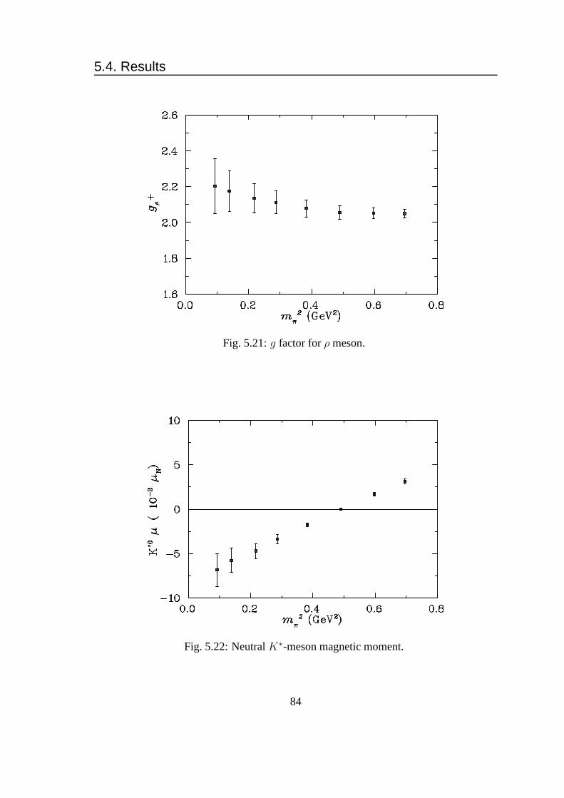
5.4. Results

Fig. 5.21:g factor forρ meson.

Fig. 5.22: NeutralK∗-meson magnetic moment.

84

5.4. Results

Fig. 5.23: Environment-dependence for light-quark contribution to vector meson mag-netic moment.

Fig. 5.24: Per quark-sector quadrupole form-factors.

85

5.4. Results

Fig. 5.25: Vector meson quadrupole form factors forρ+ andK∗+.

exist about a systematic dependence on quark mass, but the central values show no par-ticular pattern as we vary this. A negative quadrupole moment corresponds to an oblateshape - one which is compressed along the spin axis. This coincides with the calcula-tion of Alexandrouet al. [3] who observed a negative quadrupole moment for spin±1ρ-meson states in a density-density analysis. A simple quarkmodel would predict a valueof zero for this quantity, requiring an admixture ofs- andd-wave-functions in order toadmit such asymmetry. Importantly, the quadrupole form-factor is shown to be negativeat heavy quark masses, indicating that the simplest of quarkmodels is insufficient even inthis regime.

Environmental sensitivity for the quadrupole form-factor(5.26) is masked to somedegree by the amount of statistical uncertainty present in our results. Nevertheless, thecentral values show a downward trend at light quark masses. The mass-dependence plotshows that most of the contribution of theK∗ deformation is due to the up quark.

At light quark masses we see a small positive quadrupole moment for theK∗0 meson,but with little statistical significance. It would be very interesting to re-examine this withbetter statistics in order to more precisely determine the expected value at the very lightestquark masses.

86

5.4. Results

Fig. 5.26: Environment-dependence for light-quark contribution to vector mesonquadrupole form-factor.

Fig. 5.27: Quadrupole form-factor for neutralK∗ meson.

87

5.5. Conclusions

5.5 ConclusionsWe have obtained the electric, magnetic, and quadrupole form-factors (and associatedstatic quantities). Of particular interest is a firm prediction of a negative Quadrupolemoment. The ratio of quadrupole moment to mean square chargeradius is approximately1 : 30, so the deformation is small but not negligible. A larger ensemble of configurationswould enable better control of statistical uncertainties and potentially enable some work inextrapolating these quantities, but this is beyond the scope of this thesis. Further work willencompass examining the form-factors of thea1 meson, and theρ→ πγ electromagneticdecay, as well as a repeat of this work using dynamical (Full QCD) propagators.

88

6

Conclusions

We have completed a comprehensive analysis of mesons from Lattice QCD in the quenchedapproximation. Some striking results include:

• a first-ever first-principles calculation of all three of thevector meson form-factors,including the environment and mass-sensitivity of the quark contributions to eachform-factor

• a high precision calculation of the pseudoscalar meson form-factor

• a potential reconciliation of the lattice and experimentalresults for the mass of the1−+ exotic meson

• a determination that the optimal smearing prescription forlocal hybrid interpolatingfields is different from what one might natively expect from aflux-tube picture

• a calculation of meson excited states

• a comprehensive survey of conventional and hybrid meson operators

• a determination that theρ-meson is oblate, and not spherically symmetric as a naivequark model would predict. Importantly, this holds even at heavy quark masses.

It is hoped that the results of this work will be of assistanceto physicists in constrain-ing model parameters, especially as experimental values for theρ-meson are difficult tocome by due to the short lifetime of the particle. In particular, the result for the quadrupolemay help constrain the amount ofD-wave admixture in quark-model wave functions ofthe ρ, and the source-dependence results may result in more success obtaining precisecalculations of the properties of the exotic mesons.

Scope for future work lies in addressing the two main limitations of this work, bothimposed by the current state-of-the-art in computational power. These are the quenchedapproximation, whereby sea-quark loops are omitted, whichbecomes increasingly impor-tant at light quark-masses, and the finite size of our ensemble. By addressing the formerwe would greatly simplify the physical interpretation of our results, and by increasing ourensemble we would gain better control of statistical errors. In particular, a four-fold in-crease in statistics would afford us much greater insight into the environment dependenceof the light-quark contributions to the vector meson electromagnetic form-factors.

89

Bibliography

[1] M. Albanese et al. Glueball masses and string tension in lattice qcd. Phys. Lett.,B192:163, 1987.

[2] D. Alde et al. Evidence for a 1-+ exotic meson.Phys. Lett., B205:397, 1988.

[3] C. Alexandrou, P. de Forcrand, and A. Tsapalis. Probing hadron wave functions inlattice qcd.Phys. Rev., D66:094503, 2002.

[4] C. R. Allton, W. Armour, D. B. Leinweber, A. W. Thomas, andR. D. Young. Chi-ral and continuum extrapolation of partially-quenched lattice results. Phys. Lett.,B628:125–130, 2005.

[5] William Andersen and Walter Wilcox. Lattice charge overlap. i. elastic limit of piand rho mesons.Annals Phys., 255:34–59, 1997.

[6] W. Armour, C. R. Allton, D. B. Leinweber, A. W. Thomas, andR. D. Young. Unifiedchiral analysis of the vector meson spectrum from lattice qcd. 2005.

[7] R. G. Arnold, Carl E. Carlson, and Franz Gross. Polarization transfer in elasticelectron scattering from nucleons and deuterons.Phys. Rev., C23:363, 1981.

[8] William A. Bardeen, A. Duncan, E. Eichten, Nathan Isgur,and H. Thacker. Chiralloops and ghost states in the quenched scalar propagator.Phys. Rev., D65:014509,2002.

[9] C. Bernard et al. Exotic hybrid mesons from improved kogut-susskind fermions.Nucl. Phys. Proc. Suppl., 119:260–262, 2003.

[10] Claude W. Bernard et al. Exotic mesons in quenched lattice qcd. Phys. Rev.,D56:7039–7051, 1997.

[11] Sundance O. Bilson-Thompson, Derek B. Leinweber, and Anthony G. Williams.Highly-improved lattice field-strength tensor.Ann. Phys., 304:1–21, 2003.

[12] Sharada Boinepalli, Waseem Kamleh, Derek B. Leinweber, Anthony G. Williams,and James M. Zanotti. Improved chiral properties of flic fermions. Phys. Lett.,B616:196–202, 2005.

90

Bibliography

[13] Frederic D. R. Bonnet, Derek B. Leinweber, and Anthony G. Williams. General al-gorithm for improved lattice actions on parallel computingarchitectures.J. Comput.Phys., 170:1–17, 2001.

[14] Frederic D. R. Bonnet, Derek B. Leinweber, Anthony G. Williams, and James M.Zanotti. Improved smoothing algorithms for lattice gauge theory. Phys. Rev.,D65:114510, 2002.

[15] Stanley J. Brodsky and John R. Hiller. Universal properties of the electromagneticinteractions of spin one systems.Phys. Rev., D46:2141–2149, 1992.

[16] N. Cabibbo and E. Marinari. A new method for updating su(n) matrices in computersimulations of gauge theories.Phys. Lett., B119:387–390, 1982.

[17] S. U. Chung et al. Evidence for exotic j(pc) = 1-+ meson production in the reactionpi- p -> eta pi- p at 18-gev/c.Phys. Rev., D60:092001, 1999.

[18] T. Draper, R. M. Woloshyn, and Keh-Fei Liu. Electromagnetic properties of nucle-ons from lattice qcd.Phys. Lett., B234:121–126, 1990.

[19] T. Draper, R. M. Woloshyn, Walter Wilcox, and Keh-Fei Liu. Electromagnetic form-factors of hadrons.Nucl. Phys. Proc. Suppl., 9:175–180, 1989.

[20] A. R. Dzierba, R. Mitchell, A. P. Szczepaniak, M. Swat, and S. Teige. A search forj(pc) = 1-+ exotic mesons in the pi- pi- pi+ and pi- pi0 pi0 systems. 2005.

[21] S. Eidelman et al. Review of particle physics.Phys. Lett., B592:1, 2004.

[22] M. Falcioni, M. L. Paciello, G. Parisi, and B. Taglienti. Again on su(3) glueballmass.Nucl. Phys., B251:624–632, 1985.

[23] Brian J. Gough, George M. Hockney, Aida X. El-Khadra, Andreas S. Kronfeld,Paul B. Mackenzie, Bart P. Mertens, Tetsuya Onogi, and JamesN. Simone. Thelight quark masses from lattice gauge theory.Phys. Rev. Lett., 79(9):1622–1625,Sep 1997.

[24] S. Gusken. A study of smearing techniques for hadron correlation functions.Nucl.Phys. Proc. Suppl., 17:361–364, 1990.

[25] A. Holl, A. Krassnigg, P. Maris, C. D. Roberts, and S. V. Wright. Electromag-netic properties of ground and excited state pseudoscalar mesons. Phys. Rev.,C71:065204, 2005.

[26] B. L. Ioffe and A. V. Smilga. Meson widths and form-factors at intermediate mo-mentum transfer in nonperturbative qcd.Nucl. Phys., B216:373, 1983.

[27] W. Kamleh, D. B. Leinweber, and A. G. Williams. Dynamical flic fermions. Nucl.Phys. Proc. Suppl., 129:826–828, 2004.

91

Bibliography

[28] Waseem Kamleh, Derek B. Leinweber, and Anthony G. Williams. Hybrid montecarlo with fat link fermion actions.Phys. Rev., D70:014502, 2004.

[29] P. Lacock, C. Michael, P. Boyle, and P. Rowland. Orbitally excited and hybridmesons from the lattice.Phys. Rev., D54:6997–7009, 1996.

[30] P. Lacock and K. Schilling. Hybrid and orbitally excited mesons in full qcd.Nucl.Phys. Proc. Suppl., 73:261–263, 1999.

[31] D. B. Leinweber et al. Flic fermions and hadron phenomenology. 2002.

[32] D. B. Leinweber et al. Precise determination of the strangeness magnetic momentof the nucleon.Phys. Rev. Lett., 94:212001, 2005.

[33] D. B. Leinweber et al. Systematic uncertainties in the precise determination of thestrangeness magnetic moment of the nucleon.Nucl. Phys. Proc. Suppl., 141:287–294, 2005.

[34] Derek B. Leinweber and Thomas D. Cohen. Unquenching therho meson.Phys.Rev., D49:3512–3518, 1994.

[35] Derek B. Leinweber, Anthony G. Williams, Jian-bo Zhang, and Frank X. Lee. Topo-logical charge barrier in the markov-chain of qcd.Phys. Lett., B585:187–191, 2004.

[36] J. Litt et al. Measurement of the ratio of the proton form-factors, g(e) / g(m), at highmomentum transfers and the question of scaling.Phys. Lett., B31:40–44, 1970.

[37] M. Lu et al. Exotic meson decay to omega pi0 pi-.Phys. Rev. Lett., 94:032002,2005.

[38] M. Luscher and P. Weisz. On-shell improved lattice gauge theories.Commun. Math.Phys., 97:59, 1985.

[39] G. Martinelli, Christopher T. Sachrajda, and A. Vladikas. A study of ’improvement’in lattice qcd.Nucl. Phys., B358:212–230, 1991.

[40] Craig McNeile and Chris Michael. Mixing of scalar glueballs and flavour-singletscalar mesons.Phys. Rev., D63:114503, 2001.

[41] Zhong-Hao Mei and Xiang-Qian Luo. Exotic mesons from quantum chromodynam-ics with improved gluon and quark actions on the anisotropiclattice. Int. J. Mod.PHys., A18:5713, 2003.

[42] C. Michael. Hybrid mesons from the lattice. 2003.

[43] Yu. D. Prokoshkin and S. A. Sadovsky. Analysis of d wave in pi- p→ a2(0) (1320)n reaction.Phys. Atom. Nucl., 58:606–612, 1995.

[44] Stephen R. Sharpe. Quenched chiral logarithms.Phys. Rev., D46:3146–3168, 1992.

92

Bibliography

[45] Anthony W. Thomas and Adam P. Szczepaniak. Chiral extrapolations and exoticmeson spectrum.Phys. Lett., B526:72–78, 2002.

[46] S. F. Tuan, T. Ferbel, and R. H. Dalitz. Comments on evidence for a 1-+ exoticmeson.Phys. Lett., B213:537, 1988.

[47] Kenneth G. Wilson. Confinement of quarks.Phys. Rev., D10:2445–2459, 1974.

[48] Matthew Wingate, Thomas A. DeGrand, Sara Collins, and Urs M. Heller. Propertiesof the a1 meson from lattice qcd.Phys. Rev. Lett., 74:4596–4598, 1995.

[49] R. D. Young, D. B. Leinweber, and A. W. Thomas. Leading quenching effects in theproton magnetic moment.Phys. Rev., D71:014001, 2005.

[50] R. D. Young, D. B. Leinweber, Anthony W. Thomas, and S. V.Wright. Chiralanalysis of quenched baryon masses.Phys. Rev., D66:094507, 2002.

[51] J. M. Zanotti et al. Novel fat-link fermion actions.Nucl. Phys. Proc. Suppl.,109A:101–105, 2002.

[52] J. M. Zanotti et al. Spin-3/2 nucleon and delta baryons in lattice qcd.Phys. Rev.,D68:054506, 2003.

[53] J. M. Zanotti, B. Lasscock, D. B. Leinweber, and A. G. Williams. Scaling of flicfermions.Phys. Rev., D71:034510, 2005.

[54] James M. Zanotti et al. Hadron masses from novel fat-link fermion actions.Phys.Rev., D65:074507, 2002.

93

A

Data pertaining to the calculation ofmeson effective masses

These results were generated on a lattice of spacing0.128 fm. The conversion factor fromdimensionless masses to GeV is thus0.1973GeVfm/0.128fm = 1.5414GeV. We shalluse the symbols to refer to our ‘strange’ (heavy) quark. The relationship betweenκvalues and pion masses is given in Table A.1.

Table A.1:κ values, and corresponding pion masses (and uncertainties)in GeV.

iκ κ mπ

1 0.12780 0.8356(14)2 0.12830 0.7744(15)3 0.12885 0.7012(15)4 0.12940 0.6201(15)5 0.12990 0.5354(16)6 0.13025 0.4660(20)7 0.13060 0.3732(79)8 0.13080 0.3076(63)

94

Table A.2:a0 scalar meson mass fits. Column headings are in order, thekappa number,the lower and upper bounds of the fit window, the mass, error and χ2 from our analysis.

iκ tstart tend Ma σ χ2/d.o.f1 9 11 0.942468 0.008561 0.5698282 9 11 0.927582 0.010346 0.5501053 9 11 0.918652 0.013697 0.6248624 9 11 0.928701 0.020547 0.989549

Table A.3: As in Table A.2, but for theK⋆0 .

iκ tstart tend Ma σ χ2/d.o.f1 9 11 0.928457 0.010659 0.5803512 9 11 0.922306 0.011843 0.5797393 9 11 0.918652 0.013697 0.6248624 9 11 0.921341 0.016632 0.785677

Table A.4: As in Table A.2 but for conventionalπ meson operatorqγ5q.

iκ tstart tend Ma σ χ2/d.o.f1 16 26 0.542076 0.000933 1.0501072 16 26 0.502415 0.000966 1.0664333 16 26 0.454885 0.000991 0.8508274 16 26 0.402287 0.001030 0.7354605 16 26 0.347436 0.001105 0.7812976 16 26 0.302289 0.001287 0.9435197 16 26 0.242118 0.005106 0.9635538 16 26 0.199537 0.004086 0.974327

95

Table A.5: As in Table A.2 but for conventionalK meson operatorsγ5q.

iκ tstart tend Ma σ χ2/d.o.f1 16 26 0.500447 0.000975 1.0733152 16 26 0.479317 0.000983 0.9904093 16 26 0.454885 0.000991 0.8508274 16 26 0.429533 0.001014 0.8108905 16 26 0.405371 0.001059 0.8378236 16 26 0.387684 0.001123 0.9233367 16 26 0.368507 0.001670 0.8884738 16 26 0.358399 0.001425 1.156427

Table A.6: As in Table A.2 but for axial-vector pion interpolatorqγ5γ4q.

iκ tstart tend Ma σ χ2/d.o.f1 11 20 0.540293 0.001238 0.5986282 11 20 0.500503 0.001278 0.5216593 11 20 0.453187 0.001334 0.4712024 11 20 0.400662 0.001405 0.4686225 11 20 0.345862 0.001506 0.5259546 11 20 0.300941 0.001632 0.5421297 11 20 0.247653 0.002655 0.7542608 11 20 0.207590 0.004310 0.978518

Table A.7: As in Table A.2 but for axial-vectorK interpolatorsγ5γ4q

iκ tstart tend Ma σ χ2/d.o.f1 11 20 0.498332 0.001292 0.5229912 11 20 0.477352 0.001308 0.4927763 11 20 0.453187 0.001334 0.4712024 11 20 0.427686 0.001372 0.4649575 11 20 0.403065 0.001430 0.4744996 11 20 0.384818 0.001499 0.4514167 11 20 0.365499 0.001662 0.4182558 11 20 0.354341 0.001804 0.328788

96

Table A.8: As in Table A.2 but for hybrid pion interpolating field iqaγjBabj q

b.

iκ tstart tend Ma σ χ2/d.o.f1 14 20 0.540098 0.007257 0.9770182 14 20 0.499982 0.007463 0.9207853 14 20 0.452610 0.007801 0.8522794 14 20 0.400714 0.008351 0.8094585 14 20 0.346413 0.009261 0.8427816 14 20 0.301686 0.010280 1.0105597 14 20 0.248318 0.011460 1.2521998 14 20 0.194288 0.020123 0.667699

Table A.9: As in Table A.2 but for hybridK interpolating fieldisaγjBabj q

b.

iκ tstart tend Ma σ χ2/d.o.f1 14 20 0.497599 0.007541 0.9232592 14 20 0.476691 0.007634 0.8880333 14 20 0.452610 0.007801 0.8522794 14 20 0.427266 0.008067 0.8287295 14 20 0.402446 0.008470 0.8337256 14 20 0.383880 0.008929 0.9040697 14 20 0.363574 0.009673 1.0619648 14 20 0.352858 0.010477 1.067675

97

Table A.10: As in Table A.2 but for hybrid pion interpolatingfield iqaγjγ4Babj q

b.

iκ tstart tend Ma σ χ2/d.o.f1 12 26 0.545971 0.002851 0.8320752 12 26 0.506394 0.002804 0.7422633 12 26 0.458760 0.002777 0.6561494 12 26 0.405994 0.002895 0.5981555 12 26 0.350475 0.003298 0.5334176 12 26 0.304385 0.003804 0.6067927 12 26 0.249358 0.004178 1.3606968 12 26 0.208625 0.006253 1.052875

Table A.11: As in Table A.2 but for hybridK interpolating fieldisaγjγ4Babj q

b.

iκ tstart tend Ma σ χ2/d.o.f1 12 30 0.507508 0.002329 1.1035642 12 30 0.486136 0.002295 1.0532233 12 30 0.461294 0.002267 0.9842364 12 30 0.435686 0.002312 0.9370385 12 30 0.411526 0.002464 0.9419306 12 30 0.393909 0.002702 0.9725127 12 30 0.375299 0.003155 0.9576298 12 30 0.364972 0.003837 0.946693

Table A.12: As in Table A.2 but for conventionalρ-meson interpolating fieldqγjq forequal (left) and unequal (right) input quark masses.

iκ tstart tend Ma σ χ2/d.o.f1 16 22 0.727977 0.003081 1.4306452 16 22 0.703885 0.003569 1.4435633 16 22 0.677396 0.004380 1.4198434 16 22 0.651460 0.005776 1.3760145 16 22 0.628950 0.008230 1.2709346 16 22 0.613760 0.011680 1.0568547 16 22 0.600671 0.019740 0.3713438 16 22 0.610257 0.033558 0.314031

98

Table A.13: As in Table A.2 but for conventionalK∗-meson interpolating fieldsγjq.

iκ tstart tend Ma σ χ2/d.o.f1 16 21 0.702220 0.003712 1.2265652 16 21 0.690099 0.004005 1.1656993 16 21 0.676832 0.004436 1.0876624 16 21 0.663954 0.005059 1.0284795 16 21 0.652908 0.005924 0.9933266 16 21 0.645702 0.006864 0.9952037 16 21 0.638674 0.008543 0.9805318 16 21 0.639873 0.010192 0.541121

Table A.14: As in Table A.2 but for conventionalρ-meson interpolating fieldqγjγ4q.

iκ tstart tend Ma σ χ2/d.o.f1 14 19 0.730291 0.003023 1.2776652 14 19 0.706060 0.003362 1.2228233 14 19 0.679365 0.003920 1.1446714 14 19 0.652795 0.004849 1.0273375 14 19 0.629165 0.006514 0.8421736 14 19 0.611177 0.008703 0.7506877 14 19 0.591406 0.013972 1.1749888 14 19 0.571187 0.025088 0.980223

Table A.15: As in Table A.2 but for conventionalK∗-meson interpolating fieldqγjγ4q.

iκ tstart tend Ma σ χ2/d.o.f1 14 19 0.705001 0.003419 1.2126172 14 19 0.692769 0.003622 1.1864513 14 19 0.679365 0.003920 1.1446714 14 19 0.666161 0.004340 1.0936185 14 19 0.654555 0.004935 1.0251036 14 19 0.646385 0.005571 0.9778727 14 19 0.638678 0.006803 0.9405648 14 19 0.636179 0.008225 0.602243

99

Table A.16: As in Table A.2 but for Hybridρ-meson interpolatorqEjq. Error bars arelarger than signal for lightest quark mass, so this line is omitted

iκ tstart tend Ma σ χ2/d.o.f1 12 19 0.742066 0.031162 1.2364142 12 19 0.728289 0.038336 1.2178073 12 19 0.721750 0.051659 1.1259344 12 19 0.727662 0.076253 0.9499605 12 19 0.716127 0.117422 0.8872016 12 19 0.739333 0.182135 0.1790797 12 19 0.563291 0.256713 1.428986

Table A.17: As in Table A.2 but for HybridK∗-meson interpolatorqEjq. Error bars arelarger than signal for 3 lightest quark masses.

iκ tstart tend Ma σ χ2/d.o.f1 15 19 0.664570 0.079990 0.9516972 15 19 0.650558 0.096416 0.9520653 15 19 0.632943 0.126131 0.9027834 15 19 0.606679 0.184527 0.7734655 15 19 0.540478 0.326554 0.553247

Table A.18: As in Table A.2 but for Hybridρ-meson interpolatoriqaγ5Babj q

b.

iκ tstart tend Ma σ χ2/d.o.f1 12 22 0.755673 0.019271 1.3793852 12 22 0.728676 0.021446 1.3816063 12 22 0.698463 0.024823 1.3104054 12 22 0.667503 0.030086 1.1598865 12 20 0.638159 0.037711 1.2674866 12 22 0.620516 0.049515 1.2930027 12 22 0.599346 0.092423 1.2425428 12 22 0.482873 0.166664 1.150640

100

Table A.19: As in Table A.2 but for HybridK∗-meson interpolatoriqaγ5Babj q

b.

iκ tstart tend Ma σ χ2/d.o.f1 12 16 0.727823 0.026971 1.8564962 12 16 0.714623 0.027849 1.8236623 12 16 0.700190 0.029151 1.7677464 12 16 0.685916 0.031003 1.6953275 12 16 0.673457 0.033508 1.5839956 12 16 0.667761 0.036388 1.4808007 12 16 0.666913 0.041800 1.3043928 12 16 0.670980 0.048906 1.033869

Table A.20: As in Table A.2 but for Hybridρ-meson interpolatoriqaγ4γ5Babj q

b.

iκ tstart tend Ma σ χ2/d.o.f1 12 19 0.748734 0.018952 1.1619762 12 19 0.725957 0.021154 1.0548273 12 19 0.702988 0.024949 0.8687234 12 19 0.683667 0.031311 0.6501795 12 19 0.670175 0.040881 0.4778616 12 19 0.665139 0.051335 0.3816337 12 19 0.663100 0.067830 0.3225288 12 19 0.645117 0.092296 0.616030

Table A.21: As in Table A.2 but for HybridK-meson interpolatoriqaγ4γ5Babj q

b.

iκ tstart tend Ma σ χ2/d.o.f1 12 22 0.728549 0.020418 0.7629312 12 22 0.717493 0.021863 0.7093543 12 22 0.705967 0.023989 0.6375754 12 22 0.695830 0.026968 0.5677465 12 22 0.688051 0.030813 0.5149446 12 22 0.684327 0.034726 0.4874957 12 22 0.680818 0.039806 0.5518338 12 22 0.678415 0.044186 0.566844

101

Table A.22: As in Table A.2 but for pseudovector interpolating field qγ5γ4γjq with equalquark-antiquark masses.

iκ tstart tend Ma σ χ2/d.o.f1 11 16 1.032468 0.008605 0.6554862 11 16 1.012554 0.009433 0.6369953 11 16 0.991178 0.010702 0.6687744 11 16 0.970774 0.012717 0.7561785 11 16 0.954319 0.016296 0.8601636 11 16 0.943740 0.021157 1.0359397 11 16 0.944531 0.036163 1.1148808 11 16 0.964143 0.067878 0.832436

Table A.23: As in Table A.2 but for pseudovector interpolating field qγ5γ4γjq with un-equal quark-antiquark masses.

iκ tstart tend Ma σ χ2/d.o.f1 11 17 1.012299 0.009573 0.7615362 11 17 1.002074 0.010059 0.7604183 11 17 0.991242 0.010736 0.7717704 11 17 0.981190 0.011679 0.7991785 11 17 0.973582 0.013056 0.8428196 11 17 0.969448 0.014549 0.9080817 11 17 0.970464 0.018018 0.9515558 11 17 0.979468 0.023043 0.983875

102

Table A.24: As in Table A.2 but for axial-vector interpolating fieldqγ5γiq for equal quark-antiquark masses. No appropriate fit window exists for the two lightest quark-masses.

iκ tstart tend Ma σ χ2/d.o.f1 11 15 1.024361 0.007554 1.3241972 11 15 1.005865 0.008140 1.3225583 11 15 0.986890 0.009012 1.3764434 11 15 0.970093 0.010275 1.4315095 11 15 0.957989 0.012059 1.4478586 11 15 0.953572 0.014024 1.486133

Table A.25: As in Table A.2 but for axial-vector interpolating field qγ5γiq for unequalquark-antiquark masses. No appropriate fit window exists for the two lightest quark-masses.

iκ tstart tend Ma σ χ2/d.o.f1 11 15 1.005589 0.008229 1.3371632 11 15 0.996364 0.008559 1.3471393 11 15 0.986890 0.009012 1.3764434 11 15 0.978504 0.009616 1.4058115 11 15 0.972625 0.010402 1.4130366 11 15 0.971012 0.011214 1.4266397 11 15 0.974346 0.012624 1.3933978 11 15 0.983868 0.014333 1.351058

103

B

Obtaining the form of 〈r2〉

ConsiderGC(~q), the Breit-frame fourier transform of the spatial charge density

GC(~q) =

∫dx3 ei~q.~xρ(~x) , (B.1)

− ∂

∂qi

∂

∂qiGC((~q) =

∫dx3 xixie

i~q.~xρ(~x) ,

− ∂

∂qi

∂

∂qiGC((~q)

∣∣∣~q=~0

=

∫dx3 xixie

i~q.~xρ(~x)∣∣∣~q=~0

. = 〈r2〉

We can rewrite the LHS via the chain rule as

− ∂

∂qi

∂Q2

∂qi

∂

∂Q2GC(Q2)

∣∣∣Q2=0

, (B.2)

whereQ2 = −~q2 = qiqi − q0q0 = qiqi

in the Breit frame.Recall that

∂Q2

∂qi= 2qi . (B.3)

Thus we may write

〈r2〉 = − ∂

∂qi2qi

∂

∂Q2G(Q2)

∣∣∣Q2=0

. (B.4)

∂∂qiqi = 3 in 3-dimensions, so this is simply

〈r2〉 = −6∂

∂Q2G(Q2)

∣∣Q2=0

(B.5)

104

C

Source dependence results for theSU(3) β = 4.60, 20

3 × 40 lattice

105

nG Qpaths = 1 Qpaths = 3

4

8

10

Table C.1: Exotic meson Effective masses from the203×40 lattice forχ2 with nsrc = 35.Results for the heaviest four quark masses are depicted.

106

nG Qpaths = 1 Qpaths = 3

20

30

Table C.2: Exotic meson Effective masses from the203×40 lattice forχ2 with nsrc = 35.Results for the heaviest four quark masses are depicted.

107

nG Qpaths = 1 Qpaths = 3

4

8

10

Table C.3: Exotic meson Effective masses from the203×40 lattice forχ3 with nsrc = 35.Results for the heaviest four quark masses are depicted.

108

nG Qpaths = 1 Qpaths = 3

20

30

Table C.4: Exotic meson Effective masses from the203×40 lattice forχ3 with nsrc = 35.Results for the heaviest four quark masses are depicted.

109

D

Quark-level calculations

D.1 Two-point functionConsider the following two-point function for somex with x0 > 0.

χ(x; [U ])χ†(0; [U ]) (D.1)

whereχ = qa2H

abqb1 and χ†

ν = qb′

1 γ4H†b′a′

γ4qa′

2 . Here theH and H are a product ofgamma matrices and gauge functionals, the tilde indicates that these may be different atsource and sink. We shall restrict ourselves here to the caseq1 6= q2, as this is the onlycase that can be handled efficiently using lattice techniques. To minimise the necessity ofindices, let us chooseq1, q2 = u, d.

Inserting these operators, we rewrite the two-point function as

da(x)Habub(x)ub′(0)γ4H†b′a′

γ4da′

(0) (D.2)

With the spinor indices written out explicitly this is

daα(x)Hab

αβ ubβ(x) ub′

β′(0) (γ4H†b′a′

γ4)β′α′ da′

α′(0) (D.3)

One proceeds by contracting out quark pairs to construct propagators:

qaα(x)qb

β(0) = Sabαβ(x, 0)

qaα(x)qb

β(0) = −Sbaβα(0, x) . (D.4)

We denoteS(x, 0) the fermion propagator from0 to x.Eq. (D.3) corresponds to

−(Sd)a′aα′α(0, x)Hab

αβ (Su)bb′

ββ′(x, 0) (γ4H†b′a′

γ4)β′α′ . (D.5)

For Wilson-like fermions, the following property holds:

(γ5)αα′ Sabα′β′(0, x; [U ]) (γ5)β′β = Sba

βα

⋆(x, 0; [U ]) (D.6)

enabling us to write the above in terms of forward-going quark propagators as

−(γ5)αγ(Sd)aa′

γδ

⋆(x, 0, [U ]) (γ5)δα′ H

abαβ (Su)

bb′

ββ′(x, 0, [U ]) (γ4H†b′a′

γ4)β′α′ . (D.7)

Finally, we make use of the symmetry ofγ5 under transposition to rewrite this as

−(γ5)γα(Sd)aa′

γδ

⋆(x, 0, [U ]) (γ5)α′δ H

abαβ (Su)

bb′

ββ′(x, 0, [U ]) (γ4H†b′a′

γ4)β′α′ (D.8)

= −trspγ5Hab (Su)

bb′(x, 0, [U ])γ4H†b′a′

γ4γ5(Sd)aa′†

(x, 0, [U ]) (D.9)

In the case of theπ-meson, whereH = γ5, this is simplytrsp(Su)aa′

(Sd)aa′ †.

110

D.2. Electromagnetic current insertion

D.2 Electromagnetic current insertionConsider the following three-point function:

Gµ(x2, x1, 0) = χ(x2)jµ(x1)χ

†(0) (D.10)

Let us take the case whereχ = qa2Γq

a1 . Thenχ† = qa

1γ4Γ†γ4q

a2 . The electromagnetic

current can be written asjµ =∑

f Qf qfγαqf , whereQf is the electric charge of the

particular flavour involved. As above, let us takeq1, q2 asu, d to economise on indices.Inner products, and thus bra-ket expressions are linear, sowe can take this sum out to

writeGµ(x2, x1, 0) as

qudaα(x2)Γαβu

aβ(x2) u

bγ(x1)γ

µγδu

bδ(x1) u

cρ(0)

(γ4Γ

†γ4

)ρσdc

σ(0)

+ qddaα(x2)Γαβu

aβ(x2) d

bγ(x1)γ

µγδd

bδ(x1) u

cρ(0)

(γ4Γ

†γ4

)ρσdc

σ(0) .

Contracting the fermion operators to form quark propagators yields

quS⋆caσα(0, x2)Γαβ(S3)

acβρ(x2, x1, 0;µ)

(γ4Γ

†γ4

)ρσ

+ qdΓαβ(S3)⋆acβρ (x2, x1, 0;µ)ua

β(x2) ucρ(0)

(γ4Γ

†γ4

)ρσ, (D.11)

where we introduce the “ forwards 3-point propagator”:

(S3)abαβ(x2, x1, 0;µ) = qa

α(x2) qcσ(x1)γ

µσρq

cρ(x1) q

bβ(0) (D.12)

= Sacασ(x2, x1)γ

µσρS

cbρβ(x1, 0) − Sab

αβ(x2, 0)γµσρS

⋆ccρσ(x1, x1)

and the “backwards 3-point propagator”:

(S3)⋆ab

αβ(x2, x1, 0;µ) = qaα(x2) q

cσ(x1)γ

µσρq

cρ(x1) q

bβ(0) (D.13)

= S⋆caρα(x1, x2)γ

µσρS

⋆bcβσ(0, x1) + S⋆cc

ρσ(x1, x1)γµσρS

⋆baβα(0, x2)

The second terms in the forwards and backwards 3-point propagators represent dis-connected loop contributions, and in the spirit of the quenched approximation we simplydrop them. The final feature of our calculation is that we use an improved conservedvector current derived from the fermion action, rather thanthe local formulation above.

111

E

REDUCE script for calculating ratios ofthree to two-point functions

% To run type: in "Spin1FormFactors.red";% To quit: bye;%ON DIV;%% A few definitions%INDEX AL,B,RHO,LAM,SIG;VECTOR PRho,PpRho,MU,NU,PFinal,PInitial,TAU;VECTOR pplus,pzero,pminus;NOSPUR L; % Use LTR for traces.MASS PRho=mRho, PpRho=mRho;MSHELL PRho,PpRho;VECTOR Dir0,DirI,DirJ,DirK;%ORDER G1,G2,G3;%FOR ALL L,AL,B LET SIGMA(L,AL,B) = (I/2) * (G(L,AL,B)-G(L,B,AL));%FOR ALL AL,B,P,M LET SPINSUM(AL,B,P,M) =

- ( (AL.B) - (P.AL) * (P.B)/(Mˆ2) );%% Note q = p’-p matches PRD 46 2141 (1992)%FOR ALL RHO,MU,SIG,P,PP,M LET HINT(RHO,MU,SIG,P,PP,M) = - (

G1 * (RHO.SIG) * (P.MU+PP.MU)+G2 * ( (PP.RHO-P.RHO) * (MU.SIG) - (PP.SIG-P.SIG) * (MU.RHO) )-G3 * ( (PP.RHO-P.RHO) * (PP.SIG-P.SIG) * (P.MU+PP.MU) )/(2 * Mˆ2) );

%% Define vector p_0LET pzero.Dir0 = mRho;LET pzero.DirI = px_i;LET pzero.DirJ = py_i;LET pzero.DirK = pz_i;LET pzero.pzero = mRho * mRho;LET abs(mRho) = mRho;normRho := 1/(4 * eRho* mRho);

% Define vector p_+LET pplus.Dir0 = eRho;LET pplus.DirI = px + px_i;LET pplus.DirJ = py_i;LET pplus.DirK = pz_i;LET pplus.pplus = mRho * mRho;

% Define vector p_-LET pminus.Dir0 = eRho;LET pminus.DirI = px_i -px;LET pminus.DirJ = py_i;LET pminus.DirK = pz_i;LET pminus.pminus = mRho * mRho;

LET pplus.pzero = mRho * eRho;LET pminus.pzero = mRho * eRho;

LET PRho.PpRho = mRho * eRho;LET Dir0.Dir0 = 1;LET Dir0.DirI = 0;LET Dir0.DirJ = 0;LET Dir0.DirK = 0;LET DirI.DirJ = 0;LET DirI.DirK = 0;LET DirJ.DirK = 0;LET DirI.DirI =-1;LET DirJ.DirJ =-1;LET DirK.DirK =-1;

LET px_i = 0;LET py_i = 0;LET pz_i = 0;

LET eRho = SQRT(pxˆ2 + mRhoˆ2);%%ResEle := SPINSUM(MU,RHO,PFinal,mRho) * HINT(RHO,TAU,SIG,PInitial,PFinal,mRho) *

SPINSUM(SIG,NU,PInitial,mRho) * normRho;Forwards := SUB(PInitial=pzero,PFinal=pplus,ResEle);

112

Backwards := SUB(PInitial=pplus,PFinal=pzero,ResEle);Denom := SPINSUM(MU,MU,pplus,mRho) * SPINSUM(NU,NU,pzero,mRho) * normRho;%% Separation of components.%ResEle001 := SUB(MU=Dir0,NU=DirI,TAU=Dir0,Forwards) * SUB(MU=DirI,NU=Dir0,TAU=Dir0,Backwards) / SUB(MU=Dir0 ,NU=DirI,Denom);ResEle101 := SUB(MU=DirI,NU=DirI,TAU=Dir0,Forwards) * SUB(MU=DirI,NU=DirI,TAU=Dir0,Backwards) / SUB(MU=DirI ,NU=DirI,Denom);ResEle101Forwards := SUB(MU=DirI,NU=DirI,TAU=Dir0,For wards);ResEle202 := SUB(MU=DirJ,NU=DirJ,TAU=Dir0,Forwards) * SUB(MU=DirJ,NU=DirJ,TAU=Dir0,Backwards) / SUB(MU=DirJ ,NU=DirJ,Denom);ResEle203 := SUB(MU=DirJ,NU=DirK,TAU=Dir0,Forwards) * SUB(MU=DirK,NU=DirJ,TAU=Dir0,Backwards) / SUB(MU=DirJ ,NU=DirK,Denom);ResEle303 := SUB(MU=DirK,NU=DirK,TAU=Dir0,Forwards) * SUB(MU=DirK,NU=DirK,TAU=Dir0,Backwards) / SUB(MU=DirK ,NU=DirK,Denom);ResEle302 := SUB(MU=DirK,NU=DirJ,TAU=Dir0,Forwards) * SUB(MU=DirJ,NU=DirK,TAU=Dir0,Backwards) / SUB(MU=DirK ,NU=DirJ,Denom);

ResEle133 := SUB(MU=DirI,NU=DirK,TAU=DirK,Forwards) * SUB(MU=DirK,NU=DirI,TAU=DirK,Backwards) / SUB(MU=DirI ,NU=DirK,Denom);ResEle132 := SUB(MU=DirI,NU=DirJ,TAU=DirK,Forwards) * SUB(MU=DirJ,NU=DirI,TAU=DirK,Backwards) / SUB(MU=DirI ,NU=DirJ,Denom);ResEle331 := SUB(MU=DirK,NU=DirI,TAU=DirK,Forwards) * SUB(MU=DirI,NU=DirK,TAU=DirK,Backwards) / SUB(MU=DirK ,NU=DirI,Denom);

%ON FACTOR;%OUT "Spin1Product.res";ResEle001;ResEle101;ResEle101Forwards;ResEle202;ResEle203;ResEle303;ResEle302;ResEle133;ResEle132;ResEle331;ResEle101 + ResEle101 - ResEle202 - ResEle303;SHUT "Spin1Product.res";OUT T;%END;%% BYE;

113

F

Data pertaining to the calculation ofmeson form-factors

Table F.1: Rho meson mass data

iκ tstart tend Ma σ χ2/d.o.f1 17 30 0.7312 0.0030 1.2302 17 30 0.7067 0.0036 1.2093 17 30 0.6797 0.0046 1.1314 13 21 0.6537 0.0049 0.9365 13 21 0.6309 0.0056 0.7376 13 21 0.6160 0.0064 0.6107 11 20 0.6039 0.0071 0.1228 11 20 0.5982 0.0080 0.634

114

Table F.2: Pion mass data

iκ tstart tend Ma σ χ2/d.o.f1 16 24 0.5411 0.0010 1.2722 16 24 0.5013 0.0011 1.1243 16 24 0.4539 0.0011 0.9064 16 24 0.4014 0.0012 0.7495 16 24 0.3471 0.0015 0.8026 16 24 0.3020 0.0019 0.9387 16 24 0.2412 0.0042 0.6598 16 24 0.1968 0.0052 1.044

Table F.3: Strange quark contribution toK-meson form-factor.

iκ tstart tend GC σ χ2/d.o.f1 20 30 0.8178 0.0041 0.4052 20 30 0.8196 0.0045 0.3633 20 30 0.8215 0.0051 0.3294 18 30 0.8233 0.0055 0.6215 18 30 0.8249 0.0061 0.5106 18 30 0.8256 0.0068 0.5767 18 24 0.8260 0.0077 0.9718 16 24 0.8279 0.0078 0.742

Table F.4: Strange quark contribution toK∗-meson charge form-factor.

iκ tstart tend GC σ χ2/d.o.f1 20 30 0.7713 0.0070 0.8452 20 29 0.7706 0.0077 0.8533 20 28 0.7689 0.0087 0.9184 20 28 0.7657 0.0103 1.0145 20 27 0.7602 0.0124 0.9726 18 27 0.7564 0.0134 1.1837 18 25 0.7491 0.0148 0.7518 17 25 0.7454 0.0154 0.626

115

Table F.5: Up quark contribution toK-meson form-factor.

iκ tstart tend GC σ χ2/d.o.f1 20 30 0.8346 0.0042 0.6192 20 30 0.8302 0.0045 0.3463 20 30 0.8215 0.0051 0.3294 18 30 0.8126 0.0055 0.4155 18 30 0.8041 0.0062 0.3986 18 30 0.7976 0.0068 0.3617 18 24 0.7920 0.0077 0.7508 16 24 0.7910 0.0081 0.935

Table F.6: Up quark contribution toK∗-meson charge form-factor.

iκ tstart tend GC σ χ2/d.o.f1 20 30 0.7939 0.0067 0.8972 20 29 0.7828 0.0075 0.8863 20 28 0.7689 0.0087 0.9184 20 28 0.7538 0.0106 1.0165 20 27 0.7384 0.0133 1.0216 18 27 0.7271 0.0147 1.2067 18 24 0.7160 0.0172 0.8068 17 24 0.7074 0.0192 0.695

Table F.7: Up quark contribution toπ-meson charge form-factor.

iκ tstart tend GC σ χ2/d.o.f1 20 30 0.8327 0.0035 0.6492 20 30 0.8284 0.0041 0.3873 20 30 0.8215 0.0051 0.3294 18 30 0.8149 0.0061 0.4645 18 30 0.8100 0.0083 0.6166 18 30 0.8091 0.0120 0.8257 18 21 0.8123 0.0219 0.0138 16 21 0.8332 0.0301 0.646

116

Table F.8: Up quark contribution toρ-meson Charge form-factor.

iκ tstart tend GC σ χ2/d.o.f1 20 30 0.7954 0.0054 1.0212 20 29 0.7841 0.0066 0.9403 20 28 0.7689 0.0087 0.9184 20 25 0.7501 0.0122 1.1025 20 24 0.7267 0.0179 1.1166 18 23 0.7079 0.0218 1.4917 18 21 0.6830 0.0316 0.4068 17 20 0.6602 0.0398 0.914

Table F.9: Strange quark contribution toK∗ magnetic form-factor.

iκ tstart tend GM σ χ2/d.o.f1 18 24 1.4064 0.0213 0.8642 18 24 1.4125 0.0228 0.7773 18 24 1.4182 0.0252 0.6644 16 20 1.4276 0.0265 0.5805 16 20 1.4352 0.0282 0.5176 16 20 1.4378 0.0299 1.1617 15 20 1.4403 0.0314 1.2168 15 20 1.4409 0.0332 0.196

Table F.10: Up quark contribution toK∗ magnetic form-factor.

iκ tstart tend GM σ χ2/d.o.f1 18 24 1.3733 0.0187 0.7762 18 24 1.3953 0.0213 0.7123 18 24 1.4182 0.0252 0.6644 16 20 1.4453 0.0277 0.6395 16 20 1.4687 0.0314 0.6366 16 20 1.4850 0.0356 0.9207 15 19 1.5006 0.0405 0.4548 15 19 1.5127 0.0460 0.359

117

Table F.11: Up quark contribution toρ magnetic form-factor.

iκ tstart tend GM σ χ2/d.o.f1 18 24 1.3599 0.0160 1.1132 18 24 1.3889 0.0194 0.8453 18 24 1.4182 0.0252 0.6644 16 20 1.4547 0.0293 0.7165 16 20 1.4838 0.0365 0.8746 16 20 1.4961 0.0467 1.1147 15 19 1.5002 0.0601 1.0078 15 17 1.4828 0.0812 0.329

Table F.12: Strange quark contribution toK∗ quadrupole form-factor.

iκ tstart tend GQ σ χ2/d.o.f1 16 20 -0.2936 0.0280 0.2682 16 20 -0.2937 0.0299 0.2933 16 20 -0.2932 0.0327 0.3394 16 21 -0.2921 0.0371 0.4785 15 20 -0.2912 0.0411 0.5246 15 19 -0.2875 0.0456 0.1387 15 19 -0.2815 0.0527 0.3238 15 19 -0.2798 0.0603 0.439

Table F.13: Up quark contribution toK∗ quadrupole form-factor.

iκ tstart tend GQ σ χ2/d.o.f1 16 20 -0.2857 0.0264 0.4552 16 20 -0.2886 0.0288 0.3763 16 20 -0.2932 0.0327 0.3394 16 21 -0.3014 0.0389 1.2275 15 20 -0.3073 0.0447 1.1746 15 22 -0.3170 0.0520 1.2557 15 19 -0.3339 0.0646 1.0328 15 19 -0.3417 0.0791 1.024

118

Table F.14: Up quark contribution toρ quadrupole form-factor.

iκ tstart tend GQ σ χ2/d.o.f1 16 20 -0.2852 0.0224 0.5372 16 20 -0.2887 0.0263 0.3673 16 20 -0.2932 0.0327 0.3394 16 21 -0.2992 0.0438 0.7885 15 20 -0.3026 0.0560 0.6236 15 19 -0.2962 0.0744 0.4517 15 19 -0.3091 0.1116 0.5258 15 18 -0.3039 0.1652 0.626

Table F.15:Q2 values for pion (lattice units)

iκ Q2 σ1 0.091542 0.0000232 0.090542 0.0000293 0.089069 0.0000384 0.086962 0.0000545 0.084038 0.0000946 0.080797 0.0001597 0.074714 0.0005058 0.068450 0.000838

Table F.16:Q2 values forK (lattice units)

iκ Q2 σ1 0.090486 0.0000302 0.089868 0.0000333 0.089069 0.0000384 0.088124 0.0000455 0.087097 0.0000556 0.086234 0.0000657 0.085220 0.0001088 0.084666 0.000092

119

Table F.17:Q2 values forρ (lattice units)

iκ Q2 σ1 0.094518 0.0000322 0.094250 0.0000413 0.093923 0.0000584 0.093574 0.0000705 0.093236 0.0000866 0.092998 0.0001067 0.092793 0.0001238 0.092694 0.000143

Table F.18:Q2 values forK∗ (lattice units)

iκ Q2 σ1 0.094238 0.0000422 0.094091 0.0000493 0.093923 0.0000584 0.093753 0.0000645 0.093600 0.0000706 0.093497 0.0000757 0.093409 0.0000808 0.093364 0.000084

120

G

Papers by the author

1. “Light-quark FLIC fermion simulations of the 1-+ exotic mes on”J. N. Hedditch, B. G. Lasscock, D. B. Leinweber, A. G. Williams, W. Kamleh andJ. M. ZanottiPoSLAT2005, 040 (2006) [arXiv:hep-lat/0510103]Talk given at 23rd International Symposium on Lattice FieldField: Lattice 2005,Trinity College, Dublin, Ireland, 25-30 Jul 2005

2. “1-+ exotic meson at light quark masses”J. N. Hedditch, W. Kamleh, B. G. Lasscock, D. B. Leinweber, A.G. Williams andJ. M. ZanottiPhys. Rev. D72, 114507 (2005) [arXiv:hep-lat/0509106]

3. “Search for the pentaquark resonance signature in lattice QCD”B. G. Lasscocket al.Phys. Rev. D72, 014502 (2005) [arXiv:hep-lat/0503008]

4. “FLIC mesons: Hybrids and exotics”J. N. Hedditch, B. G. Lasscock, D. B. Leinweber, A. G. Williams and J. M. ZanottiNucl. Phys. Proc. Suppl.141, 43 (2005)Prepared for Workshop on QCD Down Under, Barossa Valley and Adelaide, Aus-tralia, 10-19 Mar 2004

5. “Spin-3/2 pentaquark resonance signature”B. G. Lasscocket al.PoSLAT2005, 067 (2006)Prepared for 23rd International Symposium on Lattice FieldField: Lattice 2005,Trinity College, Dublin, Ireland, 25-30 Jul 2005

6. “Lattice QCD Studies Of Pentaquarks And Exotics”B. G. Lasscocket al.Nucl. Phys. Proc. Suppl.153, 348 (2006)Talk given at Workshop on Computational Hadron Physics (Hadron Physics 13),Nicosia, Cyprus, 14-17 Sep 2005

7. “Hybrid mesons on the lattice with FLIC fermions”J. N. Hedditch, B. G. Lasscock, D. B. Leinweber, A. G. Williams and J. M. ZanottiDESY-03-208Prepared for Workshop on Gluonic Excitations, Newport News, Virginia, 14-16May 2003

8. “Hybrid meson spectrum from the FLIC action”J. N. Hedditch, D. B. Leinweber, A. G. Williams and J. M. Zanotti

121

Nucl. Phys. Proc. Suppl.128, 221 (2004) [arXiv:hep-lat/0402016]Talk given at 2nd Cairns Topical Workshop on Lattice Hadron Physics 2003 (LHP2003), Cairns, Australia, 22-30 Jul 2003

9. “Hybrid and exotic mesons from FLIC fermions”J. N. Hedditch, D. B. Leinweber, A. G. Williams and J. M. ZanottiNucl. Phys. Proc. Suppl.129, 248 (2004) [arXiv:hep-lat/0309119]Presented at 21st International Symposium on Lattice FieldTheory (LATTICE 2003),Tsukuba, Ibaraki, Japan, 15-19 Jul 2003

10. “Nucleon resonances from FLIC fermions”D. B. Leinweber, J. N. Hedditch, W. Melnitchouk, A. G. Williams and J. M. ZanottiProg. Theor. Phys. Suppl.151, 138 (2003)Prepared for Tokyo - Adelaide Joint Workshop on Quarks, Astrophysics and SpacePhysics, Tokyo, Japan, 6-10 Jan 2003

11. “Excited baryons from the FLIC fermion action”W. Melnitchouk, J. N. Hedditch, D. B. Leinweber, A. G. Williams, J. M. Zanottiand J. B. ZhangNucl. Phys. Proc. Suppl.119, 293 (2003) [arXiv:hep-lat/0210042]Submitted to 20th International Symposium on Lattice FieldTheory (LATTICE2002), Boston, Massachusetts, 24-29 Jun 2002

12. “FLIC fermions and hadron phenomenology”D. B. Leinweberet al.arXiv:nucl-th/0211014Invited plenary session talk at Conference on Quarks and Nuclear Physics (QNP2002), Julich, Germany, 9-14 Jun 2002

13. “Excited baryons in lattice QCD”W. Melnitchouket al.Phys. Rev. D67, 114506 (2003) [arXiv:hep-lat/0202022]

14. “Low-lying eigenmodes of the Wilson-Dirac operator and correlations withtopological objects”D. J. Kusterer, J. Hedditch, W. Kamleh, D. B. Leinweber and A.G. WilliamsNucl. Phys. B628, 253 (2002) [arXiv:hep-lat/0111029]

122