arX

iv:h

ep-p

h/00

0302

0v2

6 M

ar 2

000

LPT-ORSAY 00/17LTH 476

UPRF2000-05RR003.0200

Lattice calculation of 1/p2 corrections

to αs and of ΛQCD in the MOMscheme.

Ph. Boucauda, G. Burgiob, F. Di Renzob,c, J.P. Leroya,

J. Michelia, C. Parrinellob, O. Penea, C. Pittorid,

J. Rodrıguez–Quinteroa,e, C. Roiesnelf and K. Sharkeyc

a Laboratoire de Physique Theorique 1

Universite de Paris XI, Batiment 211, 91405 Orsay Cedex, FrancebDipartimento di Fisica, Universita di Parma

and INFN, Gruppo Collegato di Parma, Parma, Italy.c Dept. of Mathematical Sciences, University of Liverpool

Liverpool L69 3BX, U.K.dDipartimento di Fisica, Universita di Roma “Tor Vergata”, Roma, Italy

eDpto. de Fısica Aplicada e Ingenierıa electrica

E.P.S. La Rabida, Universidad de Huelva, 21819 Palos de la fra., Spainf Centre de Physique Theorique2 de l’Ecole Polytechnique

91128 Palaiseau Cedex, France

Abstract

We report on very strong evidence of the occurrence of power terms

in αMOM

(p), the QCD running coupling constant in the MOM scheme,by analyzing non-perturbative measurements from the lattice three-gluon vertex between 2.0 and 10.0 GeV at zero flavor. While putting

1Unite Mixte de Recherche du CNRS - UMR 86272 Unite Mixte de Recherche C7644 du CNRS

1

forward the caveat that this definition of the coupling is a gauge de-pendent one, the general relevance of such an occurrence is discussed.

We fit Λ(nf =0)

MS= 237±3 + 0

−10 MeV in perfect agreement with the resultobtained by the ALPHA group with a totally different method. Thepower correction to α

MOM(p) is fitted to (0.63 ± 0.03 + 0.0

− 0.13)GeV2/p2.

1 Introduction

The non-perturbative computation of the running QCD coupling constantαs(p) follows a two-sided goal: the large energy matching to perturbativeasymptotic QCD formula turns out to be a most direct method to predict ΛMS

from QCD first principles [1]. On the other hand, the moderate or low energybehavior of αs(p) is extremely instructive about non-perturbative propertiesof QCD. In this paper we restrict ourselves to high and intermediate energiesand consider power corrections (∼ 1/p2) to the leading asymptotic behavior.As we shall see it turns out that there is no sharp separation between theasymptotic domain and the intermediate one. The power correction, beyondthe lessons it contains by itself, greatly improves our asymptotic study and isnever negligible up to ∼ 10 GeV ! This surprising fact could only be revealedthanks to the high accuracy achieved in the present work.

The asymptotic approach has been recently followed in Ref. [2]. It isworth remarking that this matching procedure has also been developed forthe two-point Green function to the same goal [3], both matching programsleading to a consistent estimate of ΛMS. The almost two-sigma discrepancybetween the last estimate and the one obtained from Schrodinger functionalmethods [4] seems to imply that some source of systematic uncertainty re-mains uncontrolled. Furthermore the careful study of the asymptotic be-havior carried out for the gluon propagator in Refs. [3] stresses a danger:it is sometimes difficult to distinguish between the real asymptotic scaling

and a behavior mimicking asymptoticity but with a certain effective “re-scaled” Λ parameter which differs significantly from the real asymptotic one.Consequently, and in spite of the agreement between both above-mentionedestimates of ΛMS (matching two or three-point Green functions to perturba-tive formulae), we must inquire whether both are not biased by some sizablenon-perturbative effect.

2

The operator product expansion (OPE) gives a standard procedure toparametrize non-perturbative QCD effects in terms of power corrections toperturbative results. In this framework, the powers involved in the expansionare expected to be uniquely fixed by the symmetries and the dimensions of theoperators appearing in the product expansion. It should be noted that, dueto the asymptotic nature of QCD perturbative expansions, power correctionsare reshuffled between operators and coefficient functions in the OPE [5].

Since we work in Landau gauge, the gauge dependent local operatorAµAµ is allowed in the OPE [6] implying a dominant 1/p2 power correction.Indeed sizable 1/p2 corrections are present as we shall show at length in thenext section.

In a less straightforward way our result is related to another hot issue(this is the spirit of the preliminary study in [7]): the possible presence of 1/p2

terms in gauge invariant quantities such as Wilson loops [8]. Since no gluonlocal gauge invariant operator of dimension less than 4 exists it is expectedfrom OPE that the dominant power correction should be ∝ 1/p4. Thispicture has however recently been challenged [8–10]. It was pointed out thatpower corrections which are not a priori expected from the OPE may in factappear in the expansion of physical observables. Such terms may arise from(UV-subleading) power corrections to αs(p), corresponding to non-analyticalcontributions to the β-function. It is worth stressing the following. Oneknows that the perturbative analysis does not encode all the informationon the coupling. Among all that is missed, a peculiar contribution to thecoupling could result in a peculiar correction to physical observables. As amatter of fact, some evidence for an unexpected Λ2

p2 contribution to the gluon

condensate was obtained through lattice calculations in Ref. [8] (see also [11]for an early evidence of such a contribution, although the perturbative seriesinvolved was not managed up to high orders).

Let us insist: there is no direct relation between the 1/p2 correctionsfound in the present work to αs(p) in a gauge dependent scheme and thepower corrections advocated in the preceding paragraph to justify 1/p2 cor-rections to gauge independent quantities. Nobody knows how to relate agauge dependent scheme to a gauge independent one beyond the perturba-tive regime. Still, it may be that these two phenomena are not completelyunrelated and the large 1/p2 corrections found in the present work might

3

trigger some further thoughts along this line.

The paper is organized as follows: in Section 2 we explain the meaningof the lattice data, our strategy for the analysis and report the results. InSection 3 we briefly review some theoretical arguments in support of powercorrections to αs(p), illustrating the special role of the Λ2

p2 term. Finally, inSection 4 we draw our conclusions.

2 Lattice calculation of αs from Green func-

tions and power corrections

2.1 αs on the lattice

Several methods for computing αs(p) non-perturbatively on the lattice havebeen proposed in recent years [12–16]. In most cases, the goal of such studiesis to obtain an accurate prediction for αs(MZ), i.e. the running coupling atthe Z peak, which is a fundamental parameter in the standard model. Forthis reason, lattice parameters are usually tuned so as to allow the computa-tion of αs(p) at momentum scales of at least a few GeVs, where the two-loopasymptotic behavior is expected to dominate and power contributions aresuppressed.

As we shall see, however, non-perturbative power corrections cannot beneglected at energy scales as large as 10 GeV which is a sufficient reasonto consider them in the fit. As a bonus the knowledge of these power cor-rections provides us with a physically significant quantity as argued in theintroduction.

For this purpose, the best method is one where one can measure αs(p) in awide range of momenta from a single Monte Carlo data set. Indeed, a narrowenergy window does not allow to disentangle in a clear cut manner the powercorrections from unknown higher perturbative orders, and these correctionscan be mimicked by an effective ΛQCD different from the asymptotic one.

One method which fulfills the above criterion is the determination of thecoupling from the renormalized lattice three-gluon vertex function [1, 2, 16].This is achieved by evaluating two- and three-point off-shell Green’s functions

4

of the gluon field in the Landau gauge, and imposing non-perturbative renor-malization conditions on them, for different values of the external momenta.By varying the renormalization scale p, one can determine αs(p) for differentmomenta from a single simulation. Obviously the renormalization scale mustbe chosen in a range of lattice momenta such that both finite volume effectsand discretization errors are under control. Both these constraints imposetoo strict limits on the energy range if only one lattice run is used. This iswhy the procedure used in Ref. [3] combining several lattice simulations atdifferent β’s is a necessity to get a larger range of lattice momenta. The useof different volumes will also help to control finite volume artifacts.

The definition of the coupling corresponds to a momentum-subtractionrenormalization scheme in continuum QCD [17]. It should be noted thatin this scheme the coupling is a gauge-dependent quantity. As we alreadymentioned, one consequence of this fact is that 1/p2 corrections should beexpected, based on OPE considerations. For full details of the method andthe lattice calibration we refer the reader to Ref. [1, 2].

2.2 Models for power corrections and construction of

the data set

In the present work we shall not address the general problem of defining anoptimal analytic form for the coupling at all scales to which we could fitour data. For the purpose of our investigation, we shall compare the non-perturbative data for αs with simple models obtained by adding a powercorrection term of the form 1/p2 to the perturbative formula at a given or-der. This amounts to a quite raw separation between a perturbative versus

a non–perturbative contribution, the major problem of course being the pos-sible interplay between a description in terms of (non-perturbative) powercorrections and our ignorance about higher orders of perturbation theory.As crude as it may be, our recipe allows for addressing this problem, as weshall see.

In order to identify a momentum interval where our ansatz could fit thedata, one should keep in mind that the momentum range should start wellabove the location of the perturbative Landau pole, but it should nonethelessinclude low scales where power corrections may be large up to large enough

5

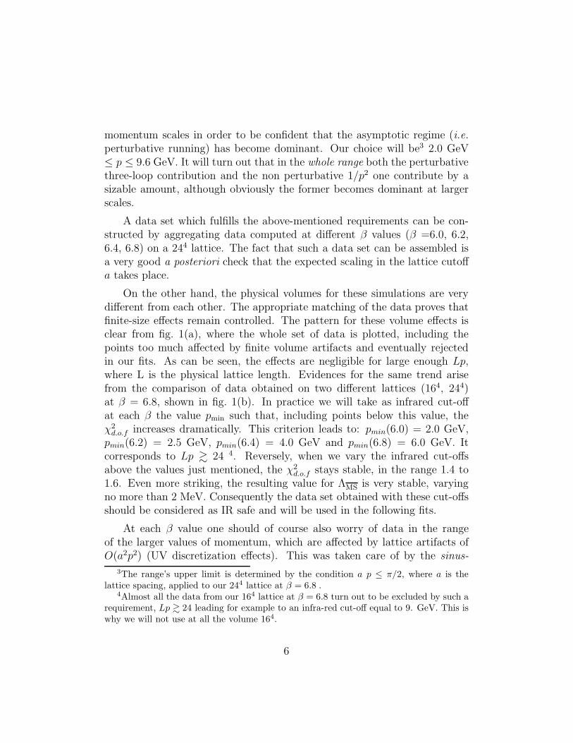
momentum scales in order to be confident that the asymptotic regime (i.e.perturbative running) has become dominant. Our choice will be3 2.0 GeV≤ p ≤ 9.6 GeV. It will turn out that in the whole range both the perturbativethree-loop contribution and the non perturbative 1/p2 one contribute by asizable amount, although obviously the former becomes dominant at largerscales.

A data set which fulfills the above-mentioned requirements can be con-structed by aggregating data computed at different β values (β =6.0, 6.2,6.4, 6.8) on a 244 lattice. The fact that such a data set can be assembled isa very good a posteriori check that the expected scaling in the lattice cutoffa takes place.

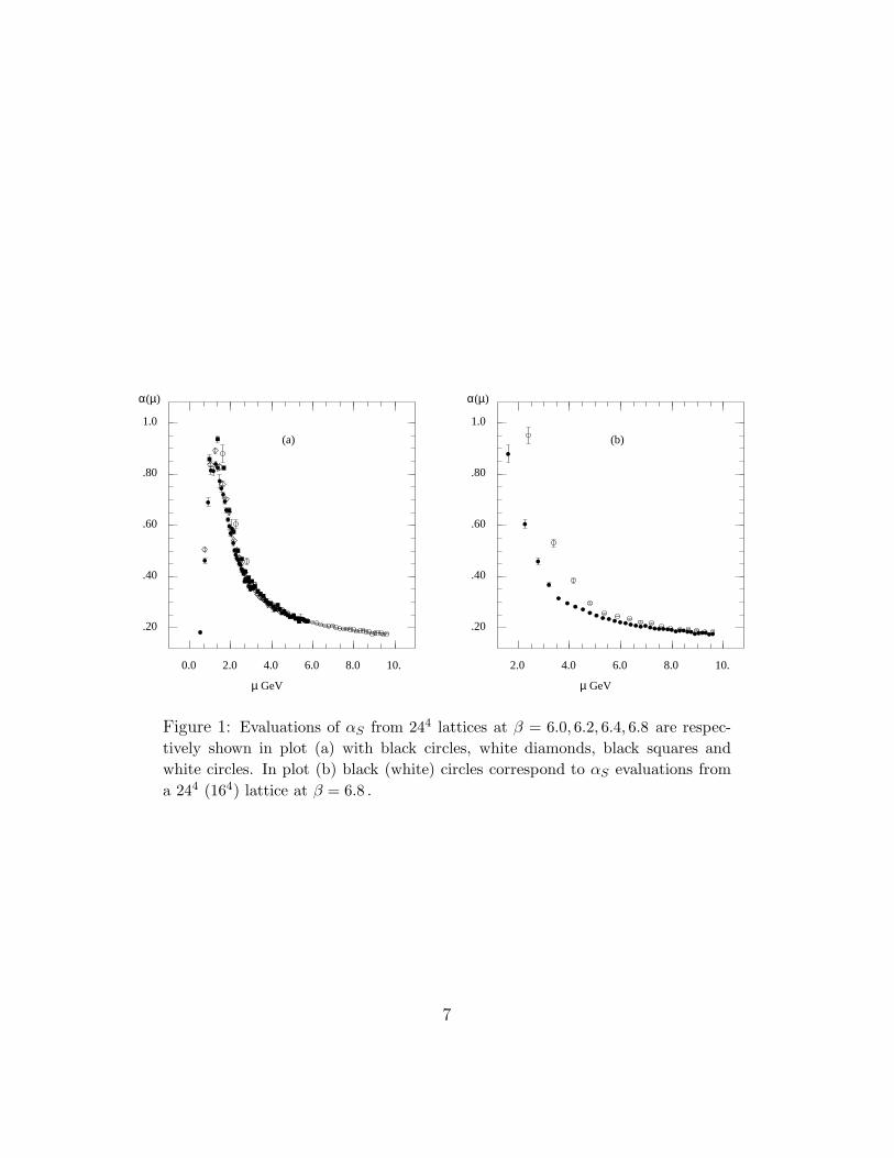
On the other hand, the physical volumes for these simulations are verydifferent from each other. The appropriate matching of the data proves thatfinite-size effects remain controlled. The pattern for these volume effects isclear from fig. 1(a), where the whole set of data is plotted, including thepoints too much affected by finite volume artifacts and eventually rejectedin our fits. As can be seen, the effects are negligible for large enough Lp,where L is the physical lattice length. Evidences for the same trend arisefrom the comparison of data obtained on two different lattices (164, 244)at β = 6.8, shown in fig. 1(b). In practice we will take as infrared cut-offat each β the value pmin such that, including points below this value, theχ2

d.o.f increases dramatically. This criterion leads to: pmin(6.0) = 2.0 GeV,pmin(6.2) = 2.5 GeV, pmin(6.4) = 4.0 GeV and pmin(6.8) = 6.0 GeV. Itcorresponds to Lp & 24 4. Reversely, when we vary the infrared cut-offsabove the values just mentioned, the χ2

d.o.f stays stable, in the range 1.4 to1.6. Even more striking, the resulting value for ΛMS is very stable, varyingno more than 2 MeV. Consequently the data set obtained with these cut-offsshould be considered as IR safe and will be used in the following fits.

At each β value one should of course also worry of data in the rangeof the larger values of momentum, which are affected by lattice artifacts ofO(a2p2) (UV discretization effects). This was taken care of by the sinus-

3The range’s upper limit is determined by the condition a p ≤ π/2, where a is thelattice spacing, applied to our 244 lattice at β = 6.8 .

4Almost all the data from our 164 lattice at β = 6.8 turn out to be excluded by such arequirement, Lp & 24 leading for example to an infra-red cut-off equal to 9. GeV. This iswhy we will not use at all the volume 164.

6

0.0 2.0 4.0 6.0 8.0 10.

.20

.40

.60

.80

1.0

µ GeV

α(µ)

(a)

2.0 4.0 6.0 8.0 10.

.20

.40

.60

.80

1.0

µ GeV

α(µ)

(b)

Figure 1: Evaluations of αS from 244 lattices at β = 6.0, 6.2, 6.4, 6.8 are respec-

tively shown in plot (a) with black circles, white diamonds, black squares and

white circles. In plot (b) black (white) circles correspond to αS evaluations from

a 244 (164) lattice at β = 6.8 .

7

improvement program which has already been described in [2], which ba-sically amounts to the substitution of the lattice momenta 2πnµ

Lwith their

O(a2p2) analogues 2asin(apµ

2). As already noticed in [2], a good rationale for

this in our gauge-fixed situation is that the gauge fixing algorithm leads tothe relation 2

asin(apµ

2) Aµ(p) = 0, while pµ Aµ does not vanish5. It should be

noticed that without this prescription the quality of almost any fit degener-ates. The relevant configurations were generated on a QH1 Quadrics systembased in Orsay (see [2]).

2.3 Fitting data to our ansatz

We now proceed to fitting the data set to our ansatz, which, we recall, is theaddition of a term proportional to 1

p2 to a given order of perturbation theory:

αs(p2) = αPert

s (p2) +c

p2. (1)

Working at three loop level, the perturbative expression for the running cou-pling constant, αPert

S (p2) requires to inverse either the unexpanded formula

Λ = Λ(c)(α)

(1 +

β1α

2πβ0+

β2α2

32π2β0

) β1

2β20

× exp

{β0β2 − 4β2

1

2β20

√∆

[arctan

( √∆

2β1 + β2α/4π

)− arctan

(√∆

2β1

)]}(2)

or the expanded one

Λ = Λ(c)(α)

(1 +

8β21 − β0β2

16π2β30

α

)(3)

5One should keep in mind that we are imposing Landau gauge.

8

where Λ(c) denotes the conventional two loops formula:

Λ(c) ≡ p exp

( −2π

β0α(p2)

)×(

β0α(p2)

4π

)−

β1

β20

; (4)

and ∆ ≡ 2β0β2−4β21 > 0 (for our MOM scheme). In the previous formula, the

use of Λ, α and β’s stands for the Λ parameter, the running coupling constant

and beta function coefficients in the particular MOM renormalization scheme.From now on we will systematically convert Λ into ΛMS using [1, 2]

ΛMS = exp(−70/66) Λ ≃ 0.346 Λ (5)

In Eqs. (2-3) the p2 dependence of α has been omitted for simplicity.

No analytical expression can exactly inverse neither unexpanded eq. (2)nor expanded eq. (3). The following formula gives an approximated solutionto the inversion of eq. (3):

α(p2) =4π

β0 t− 8πβ1

β0

log(t)

(β0 t)2

+1

(β0 t)3

(2πβ2

β0

+16πβ2

1

β20

(log2(t) − log(t) − 1)

)(6)

where t = log(p2/Λ2). On the other hand, an exact numerical inversion ofEq. (2) can be easily obtained and used to fit our data. Both ansatze, eq. (6)and the numerical inversion of eq. (2), should only differ by perturbativecontributions higher than three loops. Thus, we will fit with the two ansatze,the difference between these two predictions being considered as an estimateof the systematic uncertainty coming from the neglected perturbative orders.To make more direct the comparison with the Schrodinger functional estimateof ΛMS [4], the central value for our prediction of ΛMS should be taken fromthe fit with the exact inversion of Eq. (2)6. This yields:

6The ALPHA collaboration estimate: ΛMS

= 238(19) MeV comes from evaluatingeq. (2) for a value of αS obtained from the lattice at very high momenta.

9

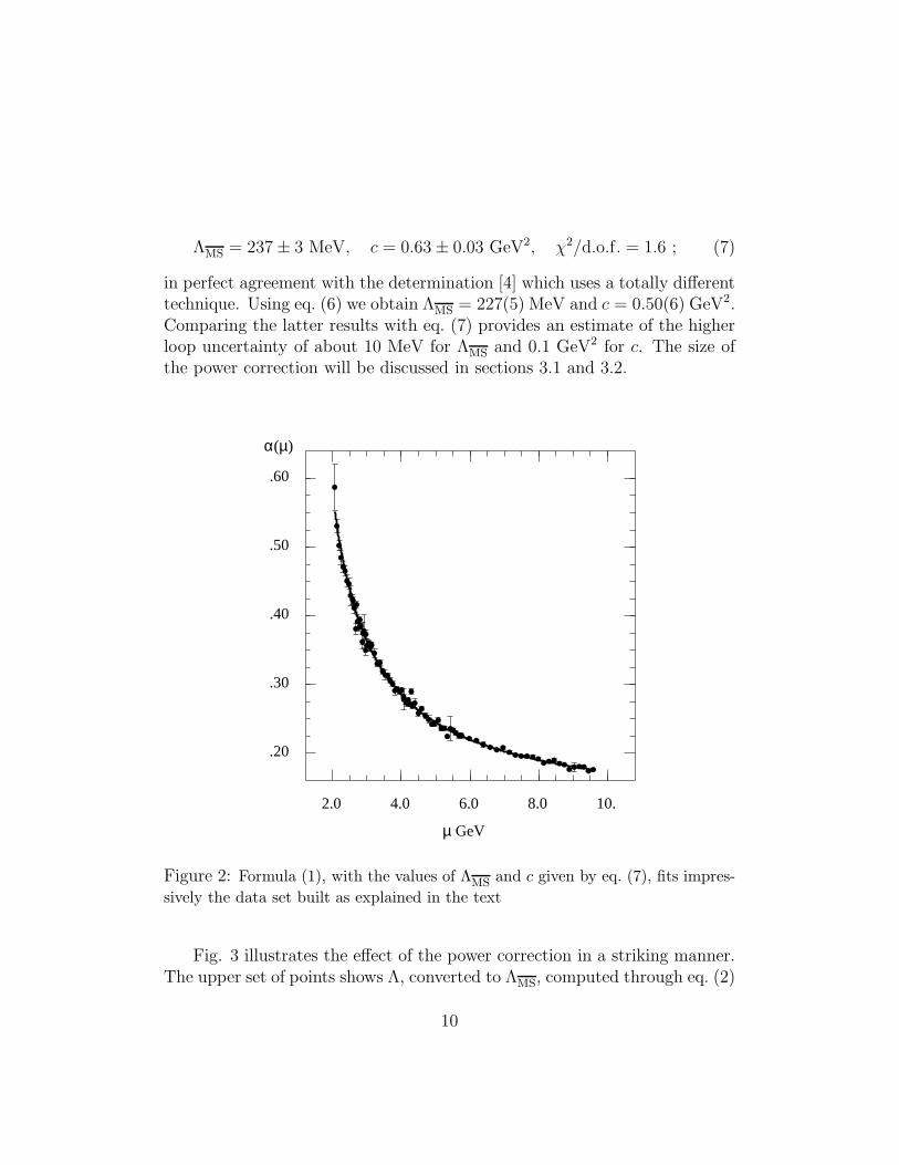
ΛMS = 237 ± 3 MeV, c = 0.63 ± 0.03 GeV2, χ2/d.o.f. = 1.6 ; (7)

in perfect agreement with the determination [4] which uses a totally differenttechnique. Using eq. (6) we obtain ΛMS = 227(5) MeV and c = 0.50(6) GeV2.Comparing the latter results with eq. (7) provides an estimate of the higherloop uncertainty of about 10 MeV for ΛMS and 0.1 GeV2 for c. The size ofthe power correction will be discussed in sections 3.1 and 3.2.

2.0 4.0 6.0 8.0 10.

.20

.30

.40

.50

.60

µ GeV

α(µ)

Figure 2: Formula (1), with the values of ΛMS and c given by eq. (7), fits impres-

sively the data set built as explained in the text

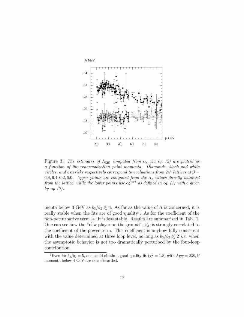
Fig. 3 illustrates the effect of the power correction in a striking manner.The upper set of points shows Λ, converted to ΛMS, computed through eq. (2)

10

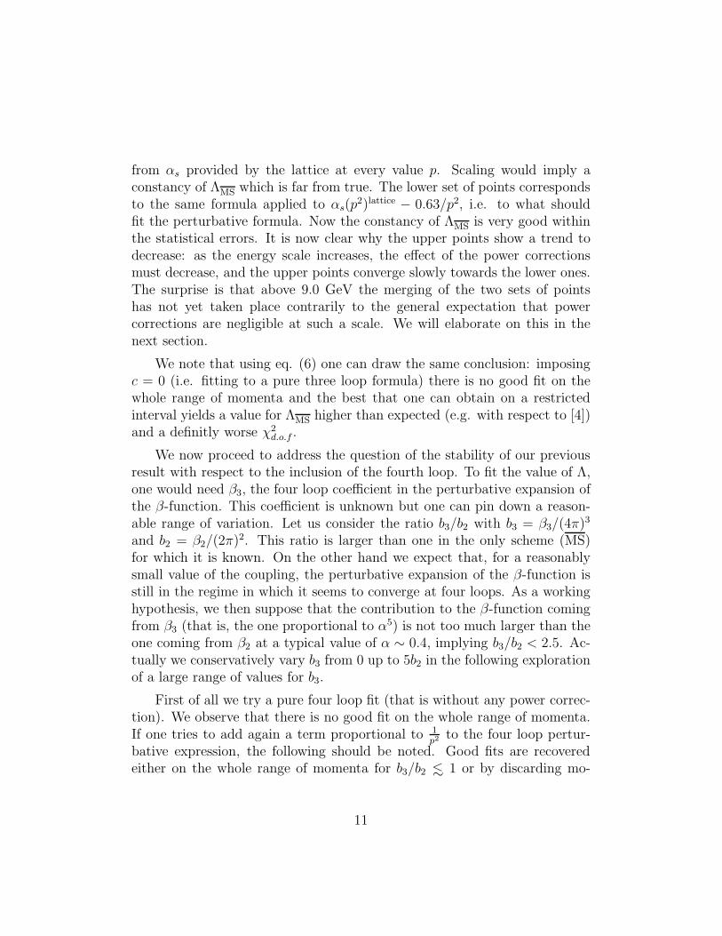
from αs provided by the lattice at every value p. Scaling would imply aconstancy of ΛMS which is far from true. The lower set of points correspondsto the same formula applied to αs(p

2)lattice − 0.63/p2, i.e. to what shouldfit the perturbative formula. Now the constancy of ΛMS is very good withinthe statistical errors. It is now clear why the upper points show a trend todecrease: as the energy scale increases, the effect of the power correctionsmust decrease, and the upper points converge slowly towards the lower ones.The surprise is that above 9.0 GeV the merging of the two sets of pointshas not yet taken place contrarily to the general expectation that powercorrections are negligible at such a scale. We will elaborate on this in thenext section.

We note that using eq. (6) one can draw the same conclusion: imposingc = 0 (i.e. fitting to a pure three loop formula) there is no good fit on thewhole range of momenta and the best that one can obtain on a restrictedinterval yields a value for ΛMS higher than expected (e.g. with respect to [4])and a definitly worse χ2

d.o.f .

We now proceed to address the question of the stability of our previousresult with respect to the inclusion of the fourth loop. To fit the value of Λ,one would need β3, the four loop coefficient in the perturbative expansion ofthe β-function. This coefficient is unknown but one can pin down a reason-able range of variation. Let us consider the ratio b3/b2 with b3 = β3/(4π)3

and b2 = β2/(2π)2. This ratio is larger than one in the only scheme (MS)for which it is known. On the other hand we expect that, for a reasonablysmall value of the coupling, the perturbative expansion of the β-function isstill in the regime in which it seems to converge at four loops. As a workinghypothesis, we then suppose that the contribution to the β-function comingfrom β3 (that is, the one proportional to α5) is not too much larger than theone coming from β2 at a typical value of α ∼ 0.4, implying b3/b2 < 2.5. Ac-tually we conservatively vary b3 from 0 up to 5b2 in the following explorationof a large range of values for b3.

First of all we try a pure four loop fit (that is without any power correc-tion). We observe that there is no good fit on the whole range of momenta.If one tries to add again a term proportional to 1

p2 to the four loop pertur-bative expression, the following should be noted. Good fits are recoveredeither on the whole range of momenta for b3/b2 <∼ 1 or by discarding mo-

11

2.0 3.4 4.8 6.2 7.6 9.0

.20

.23

.26

.28

.31

.34

GeVµ

Λ MeV

Figure 3: The estimates of ΛMS computed from αs via eq. (2) are plotted asa function of the renormalization point momenta. Diamonds, black and whitecircles, and asterisks respectively correspond to evaluations from 244 lattices at β =6.8, 6.4, 6.2, 6.0. Upper points are computed from the αs values directly obtainedfrom the lattice, while the lower points use αPert

s as defined in eq. (1) with c givenby eq. (7).

menta below 3 GeV as b3/b2 <∼ 4. As far as the value of Λ is concerned, it isreally stable when the fits are of good quality7. As for the coefficient of thenon-perturbative term 1

p2 , it is less stable. Results are summarized in Tab. 1.One can see how the “new player on the ground”, β3, is strongly correlated tothe coefficient of the power term. This coefficient is anyhow fully consistentwith the value determined at three loop level, as long as b3/b2 <∼ 2 i.e. whenthe asymptotic behavior is not too dramatically perturbed by the four-loopcontribution.

7Even for b3/b2 = 5, one could obtain a good quality fit (χ2 = 1.8) with ΛMS

= 238, ifmomenta below 4 GeV are now discarded.

12

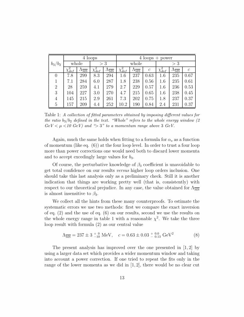
4 loops 4 loops + powerb3/b2 whole > 3 whole > 3

χ2dof ΛMS χ2

dof ΛMS χ2dof ΛMS c χ2

dof ΛMS c

0 7.8 299 8.3 294 1.6 237 0.63 1.6 235 0.671 7.1 284 6.0 287 1.8 238 0.56 1.6 235 0.612 28 259 4.1 279 2.7 229 0.57 1.6 236 0.533 104 227 3.0 270 4.7 215 0.65 1.6 238 0.454 145 215 2.9 261 7.3 202 0.75 1.8 237 0.375 157 209 4.4 252 10.2 190 0.84 2.4 231 0.37

Table 1: A collection of fitted parameters obtained by imposing different values forthe ratio b3/b2 defined in the text. “Whole” refers to the whole energy window (2GeV < µ <10 GeV) and “> 3” to a momentum range above 3 GeV.

Again, much the same holds when fitting to a formula for αs as a functionof momentum (like eq. (6)) at the four loop level. In order to trust a four loopmore than power corrections one would need both to discard lower momentaand to accept excedingly large values for b3.

Of course, the perturbative knowledge of β3 coefficient is unavoidable toget total confidence on our results versus higher loop orders inclusion. Oneshould take this last analysis only as a preliminary check. Still it is anotherindication that things are working pretty well (that is, consistently) withrespect to our theoretical prejudice. In any case, the value obtained for ΛMS

is almost insensitive to β3.

We collect all the hints from these many counterproofs. To estimate thesystematic errors we use two methods: first we compare the exact inversionof eq. (2) and the use of eq. (6) on our results, second we use the results onthe whole energy range in table 1 with a reasonable χ2. We take the threeloop result with formula (2) as our central value

ΛMS = 237 ± 3 + 0−10 MeV, c = 0.63 ± 0.03 + 0.0

− 0.13 GeV2 (8)

The present analysis has improved over the one presented in [1, 2] byusing a larger data set which provides a wider momentum window and takinginto account a power correction. If one tried to repeat the fits only in therange of the lower momenta as we did in [1, 2], there would be no clear cut

13

indication for power corrections and the effective value for Λ would turnout to be higher. What the upper momenta data really do is to single outthe asymptotic value for Λ, while deviation from asymptotia in the lowermomenta data asks for power correction rather than higher loops.

3 Discussion on the 1p2 corrections to αs(p)

Power corrections to αs(p) can be shown to arise naturally in many physicalschemes [18, 19]. The occurrence of such corrections cannot be excluded a

priori in any renormalization scheme. Even more so, as previously stated,

in a gauge dependent renormalization scheme as the MOM discussed here.Clearly, the non-perturbative nature of such effects makes it very hard toassess their dependence on the renormalization scheme, which is only veryweakly constrained by the general properties of the theory.

As discussed in the following, several arguments have been put forward inthe past to suggest that a most likely candidate for a leading power correctionto αs(p) would be the same term of order Λ2/p2 we found. Furthermore, itis worth emphasizing that this does not contradict the OPE expectation fora gauge dependent quantity.

3.1 Static quark potential and confinement

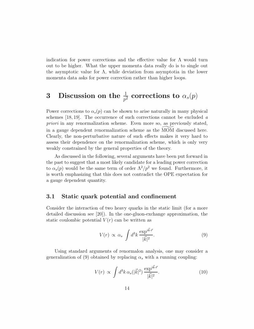
Consider the interaction of two heavy quarks in the static limit (for a moredetailed discussion see [20]). In the one-gluon-exchange approximation, thestatic coulombic potential V (r) can be written as

V (r) ∝ αs

∫d3k

expi~k·~r

|~k|2. (9)

Using standard arguments of renormalon analysis, one may consider ageneralization of (9) obtained by replacing αs with a running coupling:

V (r) ∝∫

d3k αs(|~k|2)expi~k·~r

|~k|2. (10)

14

The presence in αs(k2) of a power correction term of the form c/k2 would

generate a linear confining piece Kr in the potential V (r). It would of coursebe totally unjustified to take seriously our power correction in order to de-rive the linear potential. If we nevertheless perform this exercise to have afeeling of the scales, we get K = 2/3c ≃ 0.4 GeV2, while the usual stringtension is around 0.2 GeV2. Note that a standard renormalon analysis of(10) (see [20] for the details) reveals contributions to the potential contain-ing various powers of r, but a linear contribution is missing. This is a typicalresult of renormalon analysis: renormalons can miss important pieces of non-perturbative information.

3.2 An estimate from another lattice method

The lattice community has been made aware for some time of the possi-bility of non-perturbative contributions to the running coupling; for a cleardiscussion see [21]. Consider the “force” definition of the running coupling:

αqq(Q) =3

4r2dV (r)

dr(Q =

1

r), (11)

where again V (r) represents the static interquark potential. By keeping intoaccount the string tension contribution to V (r), which can be measured inlattice simulations, one obtains a 1/Q2 contribution, whose order of mag-nitude is given by the string tension itself. Ironically, this term has beenmainly considered as a sort of ambiguity, resulting in an indetermination inthe value of α(Q) at a given scale. From a different point of view, such aterm could be interpreted as a clue for the existence of a Λ2

p2 contribution,and it also provides an estimate for the expected order of magnitude of it,at least in one (physically sound) scheme. The same naıve exercise than inthe preceding subsection leads from eq. (11) to K = 4/3c ≃ 0.8 GeV2.

In order to make a deeper contact with what we are actually studying,one should of course keep in mind that all the preceding arguments wouldbe physically sounder in the Coulomb gauge in which the notion of forcehas a clearer meaning. In Landau gauge such a picture is far from clear.Furthermore, it is known that the interquark potential becomes close to linearat distances larger than 0.5 fm, which corresponds to a momentum smallerthan 0.4 GeV, while our 1/p2 fit only apply above 2.0 GeV i.e. at distances

15

smaller than 0.1 fm. Still, a couple of considerations are in order at this point.We note that the rough order of magnitude of the power term we found is thesame as inferred from the simple arguments from the static potential (some10−1 GeV2), even if we are in a different (UV) regime. While this could turnout to be accidental, it is nevertheless intriguing to think of some sort ofrelation. In any case, one should nevertheless note that the power correctionthat we have obtained is rather large with respect to the common wisdomof non-perturbative effects being negligible at scales such as 10.0 GeV. Afurther study of the relation between the power correction and the confiningpotential is clearly needed.

3.3 On the relation with the lattice gluon condensate

puzzle.

Having just stressed that the contribution of the power correction is ratherlarge also at a scale such as 10.0 GeV, this is a good point to go back tothe argument referring to the unexpected result of [8]. As already mentionedin the introduction, non-perturbative contribution to the running couplingcan be advocated in order to explain the Λ2/Q2 contribution to the gluoncondensate. The argument runs as follows (see [8]). From general argumentsone expects the condensate W to be written in the form

∫ Q2

0

p2dp2

Q4f(

p2

Λ2) (12)

which is based on the fact that this condensate has dimension four and isrenormalization group invariant, so that the function f(p2/Λ2), which is in-dependent on Q (for large Q), can be expressed as a function of a runningcoupling. This leads to consider the contribution coming from the large fre-quency part of the integral

∫ Q2

ρΛ2

p2dp2

Q4αs(

p2

Λ2) (13)

16

in which the function f(p2/Λ2) is taken proportional to the running coupling8.By taking into account the perturbative running coupling the IR renormaloncontribution can be obtained (see [8] for details). Again, one can consideralso contributions coming from a non–perturbative correction to the couplingof the form c/p2. From the UV limit of integration one then obtains aΛ2/Q2 contribution to W . Let us insist: this is a contribution coming froma coupling with a c/p2 correction in the UV region. While stressing againthat one can draw no definite conclusion from the following consideration,still it is worth noting that our scheme provides an example of a coupling inwhich a c/p2 correction is not negligible even at 10.0 GeV. For a discussionof possible scenarios for the result of [8] see also [22].

3.4 Landau pole and analyticity.

It is well known that perturbative QCD formulae for the running of αs in-evitably contain singularities, which are often referred to as the Landau pole.The details of the analytical structure depend on the order at which the β-function is truncated and on the particular solution chosen. The existence ofan interplay between the analytical structure of the perturbative solution andthe structure of non-perturbative effects has been advocated for a long time[23]. To illustrate this idea, consider the one-loop formula for the runningcoupling αs(p):

αs(p2) =

1

b0 log( p2

Λ2 ). (14)

Here the singularity is a simple pole, which can be removed if one redefinesαs(p) according to the following prescription:

αs(p2) =

1

b0 log( p2

Λ2 )+

Λ2

b0(Λ2 − p2), (15)

where a power correction of the asymptotic form Λ2

p2 appears. However, thesign of such a correction is the opposite of what one would expect from theresults of [8] and from the results in Section 2 (although the absolute value

8Note that higher powers would be subleading both for renormalons and for powercorrections.

17

is of the right order), so that in the end one could envisage a more generalformula for the regularized coupling:

αs(p2) =

1

b0 log( p2

Λ2 )+

Λ2

b0(Λ2 − p2)+ η

Λ2

p2. (16)

The message from (16) is that the coefficient of the power correction is notconstrained by the mere cancellation of the pole.

At higher perturbative orders one encounters multiple singularities, whichinclude an unphysical cut. There are several ways to regularize them. Inparticular, the method discussed in [23] combines a spectral-representationapproach with the Renormalization Group. The method was originally for-mulated for QED, but it has recently been extended to the QCD case [24].

4 Conclusions

We have studied the strong coupling constant estimated non perturbatively

on the lattice from Green functions in the Landau gauge using the MOMscheme. This has been performed with a large statistics of 1000 field config-urations per run and running at β = 6.0, 6.2, 6.4, 6.8. Finite volume effectsas well as finite lattice spacing effects have been carefully controlled.

We have parametrized the momentum dependence of αs using the three-loop perturbative formula plus a c/p2 term. We have obtain a good fit in theenergy range from 2.0 GeV up to 10.0 GeV. As a result of this study we find

ΛMS = 237 ± 3 + 0−10 MeV, c = 0.63 ± 0.03 + 0.0

− 0.13 GeV2, (17)

ΛMS agrees perfectly well with the result of [4] and the existence of sizablepower corrections is convincingly established. The stability of our fit has beenextensively checked.

The power correction turns out to be rather large, providing a 3% cor-rection on αs at 10.0 GeV, i.e. a 20 % correction on Λ.

Having gathered evidences for a particular scheme, one needs to addressthe issue of the general relevance of such a finding in the spirit of the dis-cussion of section 3, assessing the scheme dependence of our results. As

18

already discussed, the non-perturbative nature of power corrections makes itvery hard to formulate any theoretical procedure to estimate the impact ofscheme dependence. The best one can do at this stage is to consider differentrenormalization schemes and definitions of the coupling and gather numer-ical evidence and formal arguments supporting power corrections to αs(p).In this way, scheme-independent features may eventually be identified. Forexample, on the basis of our results, we note the following:

• Theoretical arguments suggest 1/p2 corrections both for the couplingas defined from the static potential and for the one obtained from thethree-gluon vertex. The arguments for the former case were outlinedin Sections 3.1 and 3.2. As far as the coupling from the three-gluonvertex is concerned, 1/p2 corrections appear in an OPE analysis if onekeeps into account the fact that for such a gauge dependent couplingdimension 2 condensates are expected.

• In the static potential case, the theoretical arguments also provide anestimate for the order of magnitude of the coefficient of the 1/p2 correc-tion while in the three-gluon vertex case the OPE arguments do not,suggesting instead that it may depend on the gauge. Nevertheless ,the order of magnitude of our numerical result in the Landau gauge isroughly the same as the one from the static potential case. This callsfor further investigation, which may be performed for example by at-tempting a similar calculation in a different gauge and particularly inthe Coulomb gauge in which the static potential is naturally defined.

This issue of scheme dependence could be the focus of possible futurework.

5 Acknowledgements

We thank Alain Le Yaouanc and Chris Michael for stimulating discussions.J. R-Q is indebted to Spanish Fundacion Ramon Areces for his financialsupport. F. DR acknowledges both support from PPARC and from MURST(contract 9702213582) and INFN (i.s. PR11). C. Pi. warmly thanks the“Groupe de Phys. Nucl. Th. de l’Univ. de Liege” for kind hospitality and

19

acknowledges the partial support of IISN. These calculations were performedon the QUADRICS QH1 located in the Centre de Ressources Informatiques(Paris-sud, Orsay) and purchased thanks to a funding from the Ministere del’Education Nationale and the CNRS.

References

[1] B. Alles, D. S. Henty, H. Panagopoulos, C. Parrinello, C. Pittori, D. G.Richards, Nucl. Phys. B502 (1997) 325.

[2] Ph. Boucaud, J. P. Leroy, J. Micheli, O. Pene, C. Roiesnel, JHEP 9810(1998) 017; JHEP 9812 (1998) 004.

[3] D. Becirevic, Ph. Boucaud, J. P. Leroy, J. Micheli, O. Pene, J. Rodriguez-Quintero, C. Roiesnel, Phys. Rev. D60 (1999) 094509; hep-ph/9910204(to be published in Phys. Rev. D.)

[4] S. Capitani, M. Guagnelli, M. Luscher, S. Sint, R. Sommer, P. Weisz andH. Wittig, Nucl. Phys. Proc. Suppl. 63 (1998) 153; Nucl. Phys. B544(1999) 669.

[5] For reviews and classic references see:V.I. Zakharov, Nucl. Phys. 385 1992 452;A.H. Mueller, in QCD 20 years later, vol. 1 (World Scientific, Singapore1993). B. Lautrup, Phys. Lett. 69B (1977) 109; G. Parisi, Phys. Lett.76B (1977) 65; Nucl. Phys. B150 (1979) 163; G. t’Hooft, in The Whys

of Subnuclear Physics, Erice 1977, ed A. Zichichi, (Plenum, New York1977); M. Beneke and V.I. Zakharov, Phys. Lett. 312B (1993) 340; M.Beneke Nucl. Phys. B307 (1993) 154; A. H. Mueller, Nucl. Phys. B250(1985) 327; Phys. Lett. 308B (1993) 355; G. Grunberg, Phys. Lett. 304B(1993) 183; Phys. Lett. 325B (1994) 441.

[6] For a discussion of this issue about gluon propagators, see for exampleM. Lavelle and M. Oleszczuk, Mod. Phys. Lett. A 7 (1991) 3617.

[7] G. Burgio, F. Di Renzo, C. Parrinello and C. Pittori Nucl. Phys. Proc.Suppl. 73 (1999) 623, Nucl. Phys. Proc. Suppl. 74 (1999) 388.

20

[8] G Burgio, F. Di Renzo, G. Marchesini and E. Onofri, Phys. Lett. 422B(1998) 219.

[9] R. Akhoury and V.I. Zakharov, hep-ph/9705318.

[10] G.Grunberg, hep-ph/9705290, Presented at Rencontres de Moriond 97on QCD and High Energy Hadronic Interactions; JHEP 11 (1998) 006.

[11] G.P. Lepage and P. Mackenzie, Nucl. Phys. Proc. Suppl. 20 (1991) 173.

[12] A.X. El-Khadra et al., Phys. Rev. Lett. 69 (1992) 729.

[13] M. Luscher et al., Nucl. Phys. B413 (1994) 481.

[14] G.S. Bali and K. Schilling, Phys. Rev. D47 (1993) 661.

[15] S.P. Booth et al., Phys. Lett. B294 (1992) 385.

[16] C. Parrinello, Phys. Rev. D50 (1994) 4247.

[17] See for example H.D. Politzer, Phys. Reports 14C (1974) 141.

[18] Yu.L. Dokshitzer, G. Marchesini and B.R. Webber, Nucl. Phys. 469(1996) 96

[19] S.J. Brodsky, G.P. Lepage and P.B. Mackenzie, Phys. Rev. D 28 (1983)228.

[20] R. Akhoury and V.I. Zakharov, Phys. lett. B438 (1998) 165.

[21] C. Michael, Nucl. Phys. Proc. Suppl. 42 (1995) 147.

[22] M. Beneke, Phys. Rept. 317 (1999) 1; hep-ph/0001134 and referencestherein.

[23] P. Redmond, Phys. Rev. D 112 (1958) 1404; N.N. Bogoliubov, A.A.Logunov and D.V. Shirkov, Sov. Phys. JETP 37 (1959) 805.

[24] D.V. Shirkov and I.L. Solovtsov, Phys. Rev. Lett. 79 (1997) 1209.

21