arX

iv:h

ep-p

h/97

1140

2v1

20

Nov

199

7

ROME1-1183/97TUM-HEP-296/97

Next-to-Leading Order QCD Corrections to∆F = 2 effective Hamiltonians

M. Ciuchinia, E. Francob, V. Lubiczc,

G. Martinellib, I. Scimemib and L. Silvestrinid.

a INFN, Sezione Sanita, V.le Regina Elena 299, 00161 Roma, Italy.b Dip. di Fisica, Universita degli Studi di Roma “La Sapienza” and

INFN, Sezione di Roma, P.le A. Moro 2, 00185 Roma, Italy.c Dip. di Fisica, Univ. di Roma Tre and INFN, Sezione di Roma,

Via della Vasca Navale 84, I-00146 Roma, Italyd Physik Department, Technische Universitat Munchen,

D-85748 Garching, Germany.

Abstract

The most general QCD next-to-leading anomalous-dimension ma-trix of all four-fermion dimension-six ∆F = 2 operators is computed.The results of this calculation can be used in many phenomenologi-cal applications, among which the most important are those relatedto theoretical predictions of K0–K0 and B0–B0 mixing in several ex-tensions of the Standard Model (supersymmetry, left-right symmetricmodels, multi-Higgs models, etc.), to estimates the B0

s–B0s width dif-

ference, and to the calculation of the O(1/m3b) corrections for inclusive

b-hadron decay rates.

1 Introduction

Theoretical predictions of several measurable quantities, which are relevantin K-, D- and B-meson phenomenology, depend crucially on the matrixelements of some ∆F = 2 four-fermion operators. Examples are given byFCNC effects in SUSY extensions of the Standard Model [1]-[2] (or othermodels such as left-right symmetric [3] or multi-Higgs models), by the B0

s–B0s width difference [4], and by the O(1/m3

b) corrections in inclusive b-hadrondecay rates (which actually depend on the matrix elements of several four-fermion ∆F = 0 operators [5]). In all these cases, the relevant operatorshave the form

Q = Cαβρσ(bαΓqβ)(bρΓqσ) , (1)

where Γ is a generic Dirac matrix acting on (implicit) spinor indices; α–σ arecolour indices and Cαβρσ is either δαβδρσ or δασδρβ (for the 1/m3 correctionsto the inclusive decay rates the flavour structure has the form (bq)(qb)).1

All the operators discussed in this paper appear in some “effective” the-ory, obtained by using the Operator Product Expansion (OPE). As a conse-quence, in all cases, three steps are necessary for obtaining physical ampli-tudes from their matrix elements:

i) matching of the original theory to the effective one at some large energyscale;

ii) renormalization-group evolution from the large energy scale to a lowscale suitable for the calculation of the hadronic matrix elements (typically1–5 GeV);

iii) non-perturbative calculation of the hadronic matrix elements.

In this paper we present a calculation of the two-loop anomalous dimen-sion matrix relevant for ∆F = 2 transition amplitudes. This matrix can beused for the Next-to-Leading Order (NLO) renormalization-group evolutionof the Wilson coefficient functions of the effective theory from the large tothe small energy scale, step ii). The anomalous dimension matrix includesleading and sub-leading corrections of order αs and α2

s. The calculation hasbeen performed in naıve dimensional regularization (NDR) and we give re-

1 All the formulae of this paper refer to the ∆B = 2 case. Their extension to generic∆F = 2 transitions is straightforward.

1

sults for different renormalization schemes. We have also verified that theresults obtained in different schemes are compatible. We give many detailson the calculation itself, on the definition of the renormalized operators, onthe relation between different renormalization schemes (and on the role ofthe corresponding counterterms), on the gauge invariance of the final resultsetc. We also present a list containing the contribution of all the Feynman di-agrams to the anomalous dimension matrix. The list may be useful to checkour results and for further applications. In this paper we have preferred togive the results for the one- and two-loop anomalous-dimension matrix withas many details as possible and postpone the phenomenological applicationsof the results given here to further publications. In section 5, the reader whois not interested in the theoretical and technical aspects of the calculationscan find the final results for the anomalous dimension matrix of the operatorbasis defined in eq. (13) of subsec. 2.3.

Besides presenting the results for the ∆B = 2 (∆F = 2) operators dis-cussed here, we take the opportunity to clarify several issues related to theregularization and renormalization dependence of the operators and of thecorresponding Wilson coefficients. In particular, we discuss in detail theproblems related to the precise definition of the so-called “MS schemes”,which, for composite operators, are not uniquely defined, even for a givenregularization [6]–[13]. We also examine the equivalence, and differences,of the most popular renormalization schemes, and the subtleties related toRegularization-Independent renormalization schemes (RI) [14].

The paper is organized as follows. In sec. 2, we introduce the operatorsrelevant for physical applications and define the operator basis for which theanomalous dimension matrix will be given; a general discussion on the Wilsoncoefficients, their scheme-dependence and renormalization-group evolutionwill be presented in sec. 3; the strategy for the calculation of the anomalousdimension matrix in the MS and RI schemes, to be defined below, is givenin sec. 4; the final results, together with the one-loop matrices necessaryto change renormalization scheme, are also given for some relevant cases insec. 5.

2

2 Four-fermion operators

We start this section by introducing the operators that we have in mind inview of future applications; we then illustrate the chiral and Fierz propertiesof the relevant operators which are used to derive the general form of themixing matrix.

2.1 Operators relevant for physical applications

In this subsection, we present a list of operators which enter the calculationof the physical quantities mentioned in the introduction 2:

1) FCNC in SUSY extensions of the Standard Model:

For K- and B-meson transitions, these effects have been recently an-alyzed in detail in a series of papers, see for example refs. [1]-[2]. Therelevant operators which enter the effective Hamiltonian are

Q1 = bαγµ(1 − γ5)qα bβγµ(1 − γ5)q

β ,

Q2 = bα(1 − γ5)qα bβ(1 − γ5)q

β ,

Q3 = bα(1 − γ5)qβ bβ(1 − γ5)q

α , (2)

Q4 = bα(1 − γ5)qα bβ(1 + γ5)q

β ,

Q5 = bα(1 − γ5)qβ bβ(1 + γ5)q

α ,

together with the operators Q1,2,3 which can be obtained from the op-erators Q1,2,3 by the exchange (1 − γ5) ↔ (1 + γ5).

2) The Bs–Bs width difference ∆ΓBs:

At lowest order in 1/mb, by using the OPE, the width difference ∆ΓBs

can be written in terms of two ∆B = 2 operators [4]

Q = bγµ(1 − γ5)s bγµ(1 − γ5)s ,

QS = b(1 − γ5)s b(1 − γ5)s . (3)

where, since the fermion bilinears are colour singlets (bγµ(1 − γ5)s =bαγµ(1 − γ5)s

α), the colour indices have not been shown explicitly.

2 Here and in the following we adopt the same notation as in the original papers.

3

3) Heavy-hadrons lifetimes (τB, τBs, τΛb

):

In this case, the 1/m3b corrections to the lifetime, due to Pauli interfer-

ence and W -exchange, can be written in terms of four operators [5]

OqV−A = bγµ(1 − γ5)q qγ

µ(1 − γ5)b ,

OqS−P = b(1 − γ5)q q(1 + γ5)b , (4)

T qV−A = btAγµ(1 − γ5)q qtAγµ(1 − γ5)b ,

T qS−P = btA(1 − γ5)q qtA(1 + γ5)b .

where an implicit sum over colour indices is understood. The operatorsabove are ∆B = 0 operators. They contribute to the decay rates of theB-mesons (and Λbs) not only through the so-called “eight” diagrams,but also through tadpole diagrams, in which the light- or heavy-quarkfields are contracted in a loop. These “non-spectator” diagrams mixthe operators of the basis (4) with the lower dimension operators bb,

b ~D2b, bσµνGµνb, qq, etc. The mixing matrix is, however, triangular.

Thus, it is possible to compute separately, at the NLO, the 4 × 4 sub-matrix related to the mixing of the operators appearing in (4) amongthemselves. For this sub-matrix, the Feynman diagrams entering thecalculation are the same as those relevant for the ∆B = 2 operators.

2.2 Chiral and Fierz properties of the operators

The operators considered in 1)-2) can be expressed in terms of linear com-binations of independent operators, defined by their colour-Dirac structure,belonging to some basis. In case 3), for the sub-matrix considered here,the same colour-Dirac structure (with obvious replacement of the flavour in-dices) can also be used. The choice of the basis of reference is, however,arbitrary, and different equivalent possibilities exist. We first present onepossible choice, which we find particularly convenient to discuss the chiralproperties of the operators:

QVLVL= ψα1 γµ(1 − γ5)ψ

α2 ψ

β3 γµ(1 − γ5)ψ

β4

QVLVR= ψα1 γµ(1 − γ5)ψ

α2 ψ

β3 γµ(1 + γ5)ψ

β4

QRL = ψα1 (1 + γ5)ψα2 ψ

β3 (1 − γ5)ψ

β4

4

QLL = ψα1 (1 − γ5)ψα2 ψ

β3 (1 − γ5)ψ

β4

QTLTL= ψα1 σµν(1 − γ5)ψ

α2 ψ

β3 σµν(1 − γ5)ψ

α4

QVLVL= ψα1 γµ(1 − γ5)ψ

β2 ψ

β3 γµ(1 − γ5)ψ

α4 (5)

QVLVR= ψα1 γµ(1 − γ5)ψ

β2 ψ

β3 γµ(1 + γ5)ψ

α4

QRL = ψα1 (1 + γ5)ψβ2 ψ

β3 (1 − γ5)ψ

α4

QLL = ψα1 (1 − γ5)ψβ2 ψ

β3 (1 − γ5)ψ

α4

QTLTL= ψα1 σµν(1 − γ5)ψ

β2 ψ

β3σµν(1 − γ5)ψ

α4 ,

where σµν ≡ 1/2[γµ, γν]. In (5), the flavours ψ1–ψ4 are all different and theoperators belong to irreducible representations of the chiral group. To these10 operators, we have to add those which can be obtained by exchanging left-with right-handed fields. Since, however, strong interactions cannot changechirality 3, the second set of operators does not mix with the operators definedin (5) and, because parity is conserved, the Anomalous Dimension Matrix(ADM) is the same in the two cases. Thus, in the following, we will onlyconsider the operators of eq. (5).

The previous considerations hold only if one uses a renormalization pre-scription which preserves chirality (in this respect parity is never a seriousissue). It often happens, e.g. in dimensional schemes such as the t’Hooft-Veltman MS one (HV), that the renormalization procedure violates eitherchirality, or (and) other symmetries that are manifest at the tree level, forexample the Fierz transformation properties. In order to simplify the pre-sentation of the results, we will use in the following a renormalization schemewhich preserves all the relevant symmetries (chirality and Fierz). With sucha choice, it is then sufficient to consider the basis (5). This renormaliza-tion scheme has been recently called the Regularization Independent (RI)scheme [14] (MOM in the early literature) to emphasize that the renormal-ization conditions are independent of the regularization, although they de-pend on the external states used in the renormalization procedure and onthe gauge. The RI scheme offers also a great computational advantage inthe calculation of the counterterms which contribute at the two-loop level:as demonstrated in subsec. 4.2, in this scheme it is not necessary to iden-

3 In mass-independent renormalization schemes, such as the RI schemes discussed inthis paper, chiral-symmetry relations, which can be derived in the massless theory, remaintrue also in the massive case.

5

tify and subtract separately the counterterms relative to the mixing withthe “Effervescent Operators” (EOs) which appear in dimensional regular-ization [6]–[13]. The relation between the operators renormalized in someRI scheme and, for instance, those of the standard MS schemes can thenbe easily found with a simple one-loop calculation. Finally, the RI schemeallows to use, without any further perturbative calculation, the matrix el-ements of the operators computed in lattice simulations and renormalizednon-perturbatively [15]–[17].

Chiral symmetry, and Fierz rearrangement, have further consequences,since they forbid the mixing between some of the operators appearing ineq. (5). For this reason the ADM, γ, is a block-matrix which only allowsmixing between sub-sets of the possible operators. In the convenient rep-resentation in which the operators appearing in (5) are components of rowvectors

I) ~QI ≡ (QVLVL, QVLVL

),

II) ~QII ≡ (QVLVR, QVLVR

),

III) ~QIII ≡ (QRL, QRL),

IV) ~QIV ≡ (QLL, QLL, QTLTL, QTLTL

),

Fierz rearrangement imposes the following restrictions on the form of themixing matrix:

• For set I) the structure is given by

γI ≡(AI BI

BI AI

); (6)

• If the mixing-matrix for II) is given by

γII ≡(AII BII

CII DII

), (7)

then we have

γIII ≡(DII CIIBII AII

). (8)

6

• In order to discuss Fierz rearrangement for the sector IV), we introduce

the Fierz transformation matrix for the sub-basis ~QIV

F =

0 −12

0 18

−12

0 18

00 6 0 1

2

6 0 12

0

. (9)

The anomalous dimension matrix must satisfy the relation

γIV = F γIV F (10)

The mixing matrix has a simple form in the Dirac-Fierz basis

~QF ≡ (QF1 , Q

F2 , Q

F1 , Q

F2 ) ,

QF1 = QLL +

1

4QTLTL

,

QF2 = QLL −

1

12QTLTL

, (11)

QF1 = QLL +

1

4QTLTL

,

QF2 = QLL −

1

12QTLTL

.

In this basis, the ADM can be written as

γIV ≡

AIV BIV CIV DIV

EIV FIV GIV HIV

CIV −DIV AIV −BIV

−GIV HIV −EIV FIV

(12)

In summary, we have seen that the ADM for all the operators appearingin (5) can be expressed in terms of 14 quantities, i.e. AI , BI , AII , . . ., HIV .

2.3 The Fierz basis

In the case in which ψ1 = ψ3 (or ψ2 = ψ4), not all the operators in (5) areindependent. In order to take into account the simplifications occurring in

7

this particular case, it is more convenient to give the results in the (Fierz)basis

~Q± ≡ (Q±1 , Q

±2 , Q

±3 , Q

±4 , Q

±5 )

Q±1 =

1

2

(ψα1 γµ(1 − γ5)ψ

α2 ψ

β3 γµ(1 − γ5)ψ

β4 ± (ψ2 ↔ ψ4)

)

Q±2 =

1

2

(ψα1 γµ(1 − γ5)ψ

α2 ψ

β3 γµ(1 + γ5)ψ

β4 ± (ψ2 ↔ ψ4)

)(13)

Q±3 =

1

2

(ψα1 (1 + γ5)ψ

α2 ψ

β3 (1 − γ5)ψ

β4 ± (ψ2 ↔ ψ4)

)

Q±4 =

1

2

(ψα1 (1 − γ5)ψ

α2 ψ

β3 (1 − γ5)ψ

β4 ± (ψ2 ↔ ψ4)

)

Q±5 =

1

2

(ψα1 σµν(1 − γ5)ψ

α2 ψ

β3σµν(1 − γ5)ψ

β4 ± (ψ2 ↔ ψ4)

).

In this case, the operators do not belong, in general, to irreducible repre-sentations of the chiral group, e.g. both right- and left-handed ψ2 fieldsappear in Q±

3 . The ∆B = 2 operators are obtained from the Q+i s, by taking

ψ1 = ψ3 = b and ψ2 = ψ4 = q (with this choice of flavours the Q−i vanish).

In the basis (13), the ADM has the form

γ± ≡

A± 0 0 0 00 B ±C 0 00 ±D E 0 00 0 0 F± G±

0 0 0 H± I±

, (14)

and there is no mixing between the Q+i and the Q−

i operators.

The correspondence between the operators of the basis (13) and the op-erators which are relevant for the physical applications listed in subsec. 2.1is the following

1) Q1 → Q+1 , Q2 → Q+

4 , Q3 → −1

2(Q+

4 −1

4Q+

5 ) ,

Q4 → Q+3 , Q5 → −

1

2Q+

2 ; (15)

2) Q→ Q+1 , QS → Q+

4 ; (16)

8

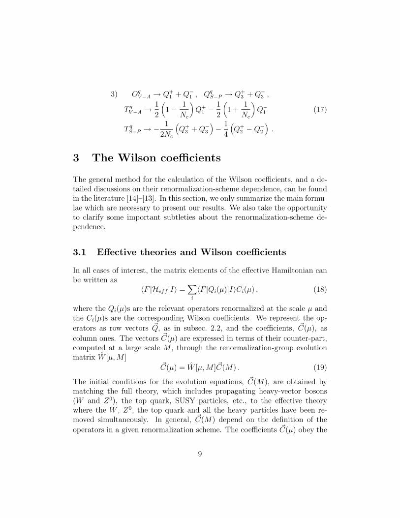
3) OqV−A → Q+

1 +Q−1 , Qq

S−P → Q+3 +Q−

3 ,

T qV−A →1

2

(1 −

1

Nc

)Q+

1 −1

2

(1 +

1

Nc

)Q−

1 (17)

T qS−P → −1

2Nc

(Q+

3 +Q−3

)−

1

4

(Q+

2 −Q−2

).

3 The Wilson coefficients

The general method for the calculation of the Wilson coefficients, and a de-tailed discussions on their renormalization-scheme dependence, can be foundin the literature [14]–[13]. In this section, we only summarize the main formu-lae which are necessary to present our results. We also take the opportunityto clarify some important subtleties about the renormalization-scheme de-pendence.

3.1 Effective theories and Wilson coefficients

In all cases of interest, the matrix elements of the effective Hamiltonian canbe written as

〈F |Heff |I〉 =∑

i

〈F |Qi(µ)|I〉Ci(µ) , (18)

where the Qi(µ)s are the relevant operators renormalized at the scale µ andthe Ci(µ)s are the corresponding Wilson coefficients. We represent the op-

erators as row vectors ~Q, as in subsec. 2.2, and the coefficients, ~C(µ), as

column ones. The vectors ~C(µ) are expressed in terms of their counter-part,computed at a large scale M , through the renormalization-group evolutionmatrix W [µ,M ]

~C(µ) = W [µ,M ] ~C(M) . (19)

The initial conditions for the evolution equations, ~C(M), are obtained bymatching the full theory, which includes propagating heavy-vector bosons(W and Z0), the top quark, SUSY particles, etc., to the effective theorywhere the W , Z0, the top quark and all the heavy particles have been re-moved simultaneously. In general, ~C(M) depend on the definition of the

operators in a given renormalization scheme. The coefficients ~C(µ) obey the

9

renormalization-group equations:

[−∂

∂t+ β(αs)

∂

∂αs+ βλ(αs)λ

∂

∂λ−γT (αs)

2

]~C(t, αs(t), λ(t)) = 0 , (20)

where t = ln(M2/µ2). The term proportional to βλ, the β-function of thegauge parameter λ(t) (for covariant gauges), takes into account the gaugedependence of the Wilson coefficients in gauge-dependent renormalizationschemes, such as the RI scheme [14, 6] 4. This term, the role of whichwill be discussed extensively in sec. 4, is absent in standard MS schemes,independently of the regularization which is adopted (NDR, HV or DREDfor example) [7]–[13]. The factor of 2 in eq. (20) normalizes the anomalousdimension matrix as in refs. [14]-[13]. To simplify the discussion, we onlyconsider the case where there is no crossing of a quark threshold when goingfrom M to µ. The relevant formulae for the general case can be found inrefs. [11]–[13].

At the next-to-leading order, we can write

W [µ,M ] = M [µ]U [µ,M ]M−1[M ] , (21)

where U is the leading-order evolution matrix

U [µ,M ] =

[αs(M)

αs(µ)

]γ(0)T /2β0

, (22)

and the NLO matrix is given by

M [µ] = 1 +αs(µ)

4πJ [λ(µ)] . (23)

By substituting the expression of the ~C(µ) given in eq. (19) in the renor-malization-group equations (20), and using W [µ,M ] written as in eqs. (21)–(23), we find that the matrix J satisfies the equation

J +β0λ

β0λ∂J

∂λ−

[J ,γ(0)T

2β0

]=

β1

2β20

γ(0)T −γ(1)T

2β0. (24)

4 In the following, we will denote by λ = 1 the Feynman gauge and λ = 0 the Landaugauge.

10

In eqs. (22) and (24), β0, β1 and β0λ are the first coefficients of the β-

functions of αs and of λ, respectively; γ(0) and γ(1) are the LO and NLOanomalous dimension matrices to be defined in sec. 4. U is determined bythe LO anomalous dimension matrix γ(0) and is therefore regularization andrenormalization-scheme independent; at this order, λ∂J/∂λ is also regular-ization (but not renormalization) scheme independent; the two-loop anoma-lous dimension matrix γ(1), and consequently J and W [µ,M ], are, instead,renormalization-scheme dependent.

3.2 Coefficient functions and scheme dependence

In this subsection, we recall some basic aspects of the calculation of theWilson coefficients and discuss in detail the issues of the regularization andrenormalization dependence of the coefficients and of the corresponding op-erators. We believe that this discussion may be useful to clarify some mis-understandings that can be found in the literature.

In order to compute the Wilson coefficients at a large energy scale µ ∼M ,we should consider the full set of current-current, box and penguin diagramsin the full theory, i.e. with propagating heavy particles, including the O(αs)corrections. To date, for the ∆F = 2 transitions, this part of the calculationhas been carried out only in the Standard Model and 2HDM cases [8]–[10].

In the full theory, the direct calculation of the current-current, box andpenguin diagrams, including O(αs) corrections has the form

〈Heff 〉 ∼ 〈 ~Q(0) T 〉 ·[~T (0) +

αs4π

~T (1)]

= 〈 ~QT (µ)〉 · ~C(µ) , (25)

where 〈 ~Q(0) T 〉 are the tree-level matrix elements and the vector ~T (1) dependson the external quark (and gluon) states chosen for the calculation. Byinserting the renormalized operators of the effective Hamiltonian, we thencompute, at order αs, the one-loop diagrams between the same external statesas in the full theory, using the same regularization. In this case we obtain 5

〈 ~Q(µ)〉 =(1 +

αs4πr)〈 ~Q(0)〉 . (26)

5 The most convenient method to define the matrix elements is by projectors on the tree-level colour-Dirac structures of the operators belonging to the four-dimensional basis [16].

11

The coefficients ~C(µ) are obtained by comparing eq. (25) with eq. (26); ifwe (formally) choose the renormalization scale µ = M , all the logarithmsrelated to anomalous dimensions of the operators disappear and

~C(M) = ~T (0) +αs4π

(~T (1) − rT ~T (0)

). (27)

~T (1) and rT depend on the external states. However their difference dependsonly on the renormalization scheme, but not on the external states. For thisreason, the dependence on the external momenta (∼ ln(−p2)) of r in ~C(M)

and ~T (1) cancels out, for details see refs. [11]–[13]. In the following r and ~T (1)

denote only non-logarithmic terms.

For given external states, and for a given gauge, the matrix r completelyspecifies the renormalization scheme (MS, RI, etc.). In this respect, all therenormalization schemes, including the MS ones, are regularization indepen-dent. The MS schemes simply amount to some specific choice of r. Thisis also demonstrated by the following observation: even when the regular-ization is specified, for example the NDR one, the so-called “MS scheme”is not unique. The renormalized operators, and consequently r, depend ingeneral on the basis chosen in the regularized theory to implement the min-imal subtraction procedure, the projectors, i.e. the definition of the EOs,etc. [11]–[13]. Thus, in order to define completely the “MS scheme”, weshould specify all the variables (regularized basis, EOs, etc.) entering thecalculation. In practice, this is equivalent to fix r, i.e. the renormalizationprescription. Summarizing, the regularization dependence must always beunderstood as a “renormalization-scheme dependence”. In all the renormal-ization schemes (both MS and RI), the same information is contained in r,once that the external states and the gauge are specified: we will then useeq. (26) to define the renormalized operators. The explicit expressions of thematrix r in the different schemes (and the corresponding states and gauge)can be found in sec. 4.

In subsection 4.2, it will be shown that the combination

G = γ(1) −[r, γ(0)

]− 2βr − 2β0

λλ∂r

∂λ(28)

is renormalization-scheme independent. It can be easily shown that a conse-quence of eq. (28) is the independence of the combination

JRI = J + rT (29)

12

of the renormalization scheme (but not of the external states and, in general,of the gauge on which r is computed), see also refs. [14]–[13].

The independence of JRI (and of G) of the renormalization scheme meansthe following. As mentioned above, for given external states, and in a givengauge, we compute the matrix element of the renormalized operators. Theseoperators are renormalized in some scheme, for example one of the possibleMS schemes. If we change scheme, r and J will accordingly change, whilstJRI will remain the same. Using eqs. (24) and (28), we find indeed

JRI +β0λ

β0λ∂JRI∂λ

−

[JRI ,

γ(0)T

2β0

]=

β1

2β20

γ(0)T −GT

2β0. (30)

The scheme independence of G and γ(0) guarantees the independence of thesolution of eq. (30). In turn, this implies the renormalization-scheme inde-pendence of the matrix JRI . Note also that, since JMS is gauge independent,

∂JRI/∂λ = ∂rTMS/∂λ.

The renormalization-invariant properties discussed above can be used tointroduce schemes which respect all the symmetries of the tree-level theory.Using eqs. (21)–(23) and (27), we introduce a new set of Wilson coefficients~C ′(M)

~C(µ) = M [µ] U [µ,M ] N−1[M ] ~C ′(M) , (31)

where M [µ] has been defined in eq. (23) and

N [M ] = 1 +αs(M)

4π

(J + rT

), ~C ′(M) = ~T (0) +

αs4π

~T (1) . (32)

In the above equations we have neglected higher order terms in αs. By asuitable change of the renormalization scheme, corresponding to

~V T (µ) = ~QT (µ)

(1 −

αs(µ)

4πrT), (33)

and M [µ] → N [µ] one gets

~C ′(µ) = N [µ]U [µ,M ]N−1[M ] ~C ′(M) . (34)

Equation (34) has the following interpretation: it corresponds to the generalexpression (21), with the matrices M [µ] and M [M ] given in terms of JRI ,

13

which satisfies eq. (30). In this renormalization scheme, G = γ(1)RI , since r =

rRI = 0. Clearly, the result is independent of the renormalization scheme ofthe original operators ~Q(µ). The scheme dependence is implicitly containedin the states and the gauge on which r is computed. Thus, in the following,we will call FRI (LRI) the scheme with matrix elements computed in theFeynman (Landau) gauge.

A remark is in order at this point. In refs. [18]–[20], for ∆B = 1 transi-tions, the authors used the so-called regularization-scheme-independent co-efficients (corresponding to our C ′(µ)) introduced in ref. [11] 6 and computedin ref. [18]. In this reference, the preference for using this particular renor-malization scheme was justified with the argument that also the operatormatrix elements computed with factorization (and used in [18]) are schemeindependent. It was therefore argued that the regularization-independentcoefficients are more suited to obtain the physical amplitudes. This argu-ment is clearly illusory: the coefficients, though regularization independent,depend on the external states and on the gauge at which the renormaliza-tion conditions have been imposed. There is no way to match the externalquark and gluon states, used in the perturbative calculation of the Wilsoncoefficients, to the hadronic states on which the operator matrix elementsare computed (not to speak about gauge invariance). A similar argumentapplies to the scheme used in ref. [21], where the authors try to get rid ofthe µ dependence of the non-leptonic amplitudes computed with factoriza-tion. In any case, in the absence of a consistent calculation in which boththe coefficients and the matrix elements of the operators are computed withthe same renormalization, a preferred scheme does not exist.

4 Anomalous dimensions at one and two loops

In this section we recall the procedure for the calculation of the anomalousdimension matrix γ in dimensional regularization. The section is divided intwo parts: in the first part, we introduce the general formulae which definethe anomalous dimension matrix, in the second we give the practical recipe

6Indeed the renormalization scheme of ref. [11] has never been completely specified,because the external states, on which the renormalization conditions were imposed, havenot been given explicitly.

14

to compute it at the NLO.

4.1 General definitions and scheme dependence

The ADM for the operators appearing in the effective theory is given by thematrix

γ = 2 Z−1µ2 d

dµ2Z , (35)

where Z ≡ Z(αs, λ), defined by the relation

~Q = Z−1 ~QB , (36)

gives the renormalized operators in terms of the bare ones. λ is the renormal-ized gauge parameter on which, in general, Z may depend, see for exampleref. [6]. Note that in refs. [7]–[13] the dependence on the gauge parameter wasignored because, in MS schemes, Z is gauge independent. In this work, sincewe will compare anomalous-dimension matrices between schemes in which Zcan be gauge dependent, such as the RI scheme, this dependence has to betaken explicitly into account.

In dimensional regularization, using eq. (35), one gets

γ = 2 Z−1

[(−ǫαs + β(αs))

∂

∂αsZ + λβλ(αs)

∂

∂λZ

], (37)

where ǫ = (4 − D)/2. β(αs) and βλ(αs) are the β functions which gov-ern the evolution of the effective coupling constant and renormalized gaugeparameter λ, respectively

µ2dαsdµ2

= β(αs) , µ2 dλ

dµ2= λβλ(αs) , (38)

with

β(αs) = −β0α2s

4π− β1

α3s

(4π)2+O(α4

s) , βλ(αs) = −αs4πβ0λ +O(α2

s) . (39)

β0, β1 and β0λ are given by

β0 =(11N − 2nf )

3, β1 =

34

3N2 −

10

3Nnf −

(N2 − 1)

Nnf ,

β0λ = −

N

2

(13

3− λ

)+

2

3nf , (40)

15

where nf is the number of active flavours. The strong coupling constantαs and the gauge parameter λ are renormalized in the MS scheme. Thisdoes not imply that also the operators must be computed in MS, becausethe definition of the composite operators is an independent step that hasnothing to do with the procedure which renormalizes the parameters of thestrong-interaction Lagrangian.

From eq. (37), by writing γ and Z as series in the strong coupling constant

γ =αs4π

γ(0) +α2s

(4π)2γ(1) + · · · , (41)

and

Z = 1 +αs4πZ(1) +

α2s

(4π)2Z(2) + · · · , (42)

we derive the following relations

γ(0) = −2ǫZ(1) (43)

and

γ(1) = −4ǫZ(2) − 2β0Z(1) + 2ǫZ(1)Z(1) − 2β0Z

(1) − 2β0λλ∂Z(1)

∂λ. (44)

We can expand Z(i) in eqs. (43) and (44) in inverse powers of ǫ

Z(i) =i∑

j=0

(1

ǫ

)jZ

(i)j . (45)

The requirement that anomalous dimension is finite as ǫ → 0 implies arelation between the one- and two-loop coefficients of Z (note that in all the

regularizations Z(1)1 is gauge invariant for gauge invariant operators)

4Z(2)2 + 2β0Z

(1)1 − 2Z

(1)1 Z

(1)1 = 0 , (46)

which can be used as a check of the calculations. In addition, from theeqs. (43) and (44) we obtain

γ(0) = −2Z(1)1 (47)

16

and

γ(1) = −4Z(2)1 − 2β0Z

(1)0 + 2(Z

(1)1 Z

(1)0 + Z

(1)0 Z

(1)1 ) − 2β0

λλ∂Z

(1)0

∂λ. (48)

Thus, it is sufficient to compute the pole and finite part of Z(1) and thesingle pole of Z(2), together with β0 and β0

λ, in order to obtain the two-loopanomalous dimension. Note that the last term in eq. (48) is absent in refs. [7]–[13]. Eq. (48) tells us how to derive γ(1). In dimensional regularizations, suchas HV, NDR or DRED, the calculation is complicated by the presence of theso-called “effervescent” operators, which appear in the intermediate steps ofthe calculation [6, 7]. The EOs are independent operators which are presentin D dimensions but disappear in the physical basis of the 4-dimensionaloperators. Because of the presence of the EOs, the products of the matricesZ

(i)j in eq. (48) have to be done by summing indices over the full set of

operators, including the EOs. Only at the end of the calculation we canrestrict the set of operators to thoses of the physical 4-dimensional basis.As explained below, the identification of the EOs, and of the correspondingmixing matrix, can be completely avoided in RI schemes.

4.2 Extraction of the the one- and two-loop anomalous

dimension matrix

We now derive the general expression of the coefficients Z(i)j s in an arbitrary

renormalization scheme, as obtained by using dimensional regularization.The derivation is general and, with trivial modifications, holds also withother regularizations, such as for example the lattice one [14]. Let us consider

the matrix elements of generic bare operators, denoted as ~QB, computed in acovariant gauge, between assigned quark and gluon external states. We definethe matrix elements of ~QB as the 1PI bare Green functions ΓQB

multipliedby the renormalization constants of the external fields

〈 ~QB〉 = Z−2ψ ΓQB

, (49)

where Zψ will be defined below. By calling α0 the dimensionless bare couplingconstant, for p2 = −µ2, where p2 denotes generically the squared momentum

17

of the external states, we have 7

〈 ~QB〉 =

[1 +

α0

4π

(A0 +

A1

ǫ

)

+(α0

4π

)2(B0 +

B1

ǫ+B2

ǫ2

)]〈 ~Q(0)〉 . (50)

〈 ~Q(0)〉 are the tree-level matrix elements of all the operators of the regularizedtheory, including the EOs. At one loop, for gauge-invariant operators, thematrix A1 is gauge and regularization independent, whilst A0 can be writtenin the form

A0(λ0) = A0(0) + λ0∂A0

∂λ0(51)

where λ0 is the bare gauge-parameter. Note that also ∂A0/∂λ0 is regulariza-tion independent.

In eq. (50), we substitute the bare parameters α0 and λ0 with theirrenormalized counter-parts, according to

λ0 = λ

(1 −

αs4π

β0λ

ǫ+ . . .

), α0 = αs

(1 −

αs4π

β0

ǫ+ . . .

). (52)

At the NLO, and taking into account that A1 is gauge invariant, we canignore all other terms which relate the bare and the renormalized couplingconstant and gauge parameter.

For a given, generic renormalization scheme, we can write the followingrelation between matrix elements

〈QR〉 = Z−1〈QB〉 =(1 +

αs4πr)〈Q(0)〉 , (53)

where the matrix r defines the renormalization scheme. With a little algebra,a comparison of eqs. (50), (52) and (53) gives the mixing matrix Z in terms

7 When working in the MS scheme, it is convenient to express the poles in terms of1/ǫ = 1/ǫ− γE + ln(4π), where γE is the Euler gamma. The formulae below are valid alsoin the MS scheme if one interprets 1/ǫ as 1/ǫ.

18

of A0, . . . B2 (we list only the terms which are needed at the NLO)

Z(1)0 = A0 − r , Z

(1)1 = A1 ,

Z(2)1 = B1 − A1r − β0A0 − β0

λλ∂A0

∂λ, (54)

Z(2)2 = B2 − β0A1 .

γ(1) is then readily obtained by substituting the relations (54) in eq. (48). Tothis purpose, we express the regularization and renormalization-independentcombination (obviously γ(0) = −2A1)

G = γ(1) −[r, γ(0)

]− 2β0r − 2β0

λλ∂r

∂λ(55)

in terms of the matrices A0, . . . B2,

G = −4

[B1 −

1

2

(A1A0 + A0A1

)−

1

2β0A0 −

1

2β0λλ∂A0

∂λ

]. (56)

Equation (56) demonstrates that G is renormalization-scheme independentsince the r.h.s. does not depend on r. G is also regularization independentas the following, simple argument demonstrates. Let us compute the matrixelements of the renormalized operators using two different regularizations,but the same external quark and gluon states and in the same gauge. Irre-spectively of the regularization used in the calculations, we can define theoperators in the same renormalization scheme in terms of the mixing matrixr in eq. (53). Since the renormalized operators are the same, they obey thesame renormalization-group equations. Thus, not only r, but also γ(1) is thesame in the two cases. This demonstrates that the l.h.s. of eq. (56) is alsoregularization independent.

Note that the last term of eq. (55) is absent in refs. [7]–[13]. This isbecause in all MS schemes the derivative ∂r/∂λ is regularization invariant, i.e.it is the same for two different MS regularizations. Thus, in these schemes,the difference between the two-loop ADMs is given by:

∆γ(1) =[∆r, γ(0)

]+ 2β0∆r (57)

On the other hand, the combination G depends on the external states usedin the calculation, and on the gauge, because r depends on these variables.

19

The RI scheme is defined, for given external states and at a fixed gauge, bythe condition r = 0. Thus, in this scheme, G coincides with the two-loopanomalous dimension.

Equation (56) provides also a practical method to compute the ADM interms of the one-loop matrices A1 and A0 and of the two-loop pole term B1.In refs. [7] and [13], it was demonstrated that the equation which allows tocompute γ(1) in terms of the one- and two-loop renormalization matrices isvalid diagram-by-diagram. In ref. [13] it was also shown that the relations be-tween the anomalous dimensions in different regularizations/renormalizationscan also be established on a diagram-by-diagram basis. Using these obser-vations, and eq. (56), we give the recipe to obtain in a very simple way the

anomalous dimension matrix in the RI scheme, γ(1)RI :

i) Choose the set of external states, and the gauge, which define the RIscheme of interest.

ii) Compute a given two-loop diagram where the bare operator is inserted.

iii) Subtract to it the result obtained by substituting, to any internal subdi-agram, one half of the amplitude of the corresponding one-loop diagramcomputed at p2 = −µ2:

1

2

αs4π

(A0 +

A1

ǫ

)〈 ~Q(0)〉 , (58)

i.e. one half of the contribution of the subdiagram to A0 and A1.

iv) When the internal subdiagram contributes to the renormalization of αsand of the gauge parameter λ, apply iii) by inserting, in the two-loopdiagram, only the divergent part of one-loop diagram (always with afactor 1/2). This rule corresponds to the choice of renormalized αs andλ in the MS scheme.

v) The coefficient of the single pole obtained from steps i) - iv) is thecontribution of the given two-loop diagram to the combination (56).

With this procedure, we do not need to isolate the EOs from the operatorsof the 4-dimensional basis. The reason is two-fold. On the one hand, in the

20

RI scheme, the counterterms corresponding to the EOs and to the operatorsof the 4-dimensional basis (i.e. the combination A1A0 + A0A1 of eq. (56))are both subtracted with the same factor 1/2. As shown in eq. (61) below,in the MS scheme, instead, different factors, namely 1 and 1/2, enter thesubtraction for the 4-dimensional and effervescent counterterms. Moreover,the subtracted diagrams, as obtained from steps i) to v), only contain simplepoles or finite terms, while the double poles completely cancel out. Thus,the projection on the physical 4-dimensional basis cannot give rise to furthersingle-pole terms due to the EOs.

For completeness, we now give the definition of the quark wave-functionrenormalization which we used in the RI scheme. We introduce the two-pointGreen function, computed in the same gauge as the RI scheme at hand,

Γψ(p2) =

i

48tr(γµ∂S(p)−1

∂pµ

), (59)

where the trace is taken over colour and spin indices. The renormalizationcondition for the quark fields is given by

Z−1ψ (µ2)Γψ(p

2 = µ2) = 1 . (60)

Note that, in the calculation of the four-point Green functions, in any givenscheme, different choices of the wave-function renormalization correspondto different choices of the quark external states. Thus, they also imply, inpractice, different definitions of the renormalized operators. Obviously, allthese choices are equivalent in principle, and they do not affect the calculationof the physical quantities at the order we are working. In the RI scheme,however, the specific choice of eq. (60) has the advantage that the vector andaxial-vector currents, renormalized according to the same rules used for thefour-fermion operators, satisfy automatically the relevant Ward identities.This is true for all the regularizations used in the intermediate steps andthus provides a useful check of the calculations. The validity of the Wardidentities among renormalized quantities is not a-priori guaranteed, and itdoes not occur, for instance, in the HV- or DRED-MS schemes, because ofthe chiral symmetry breaking induced by the regularization. In the lattercases, the finite one-loop coefficient, entering the forward matrix elementof the axial-vector current, does not vanish. These finite corrections are

21

compensated, in the evolution equation of the Wilson coefficients, by a termappearing in the two-loop current anomalous dimension.

In order to obtain the anomalous dimension in the MS scheme, one canproceed in two ways. The first was explained in refs. [7]–[13] and the detailswill not be given here. It is based on the relation

γ(1)

MS= −4

[B1 −

(A1

) (A0

)−

1

2

(A1

) (A0

)− β0A0 − β0

λλ∂A0

∂λ

]. (61)

which can be derived from eqs. (55) and (56) by using rMS = A0. In eq. (61),we denoted as Ai the matrix elements restricted to the operators of thefour-dimensional basis, and as Ai those connecting the operators of the four-dimensional basis with the effervescent ones. γ

(1)

MSis obviously the restricted

matrix. The second method to obtain γ(1)

MS, is by using the relation

γ(1)RI = γ

(1)

MS− 2

(A1A0 − A0A1

)− 2β0A0 − 2β0

λλ∂A0

∂λ(62)

which follows from eqs. (56) and (61) and it is also valid diagram by diagram.Note that the change of scheme in eq. (62) is equivalent to the substitution

JMS = JRI − rTMS

(63)

discussed in eq. (29) of subsec. 3.2.

4.3 Checks of the calculation

In this subsection, we illustrate several checks that have been made in orderto verify the correctness of our calculations:

• in the NDR-MS renormalization scheme, the ADM of the operatorsQ±1 ,

Q±2 and Q±

3 can be extracted from the results of refs. [11, 13]. Theyagree with the results presented in this paper;

• we have computed the anomalous dimension matrix both in MS and inRI and verified that the result satisfy eq. (55), i.e. that we get exactlythe same G in the two schemes;

22

• by computing the two-loop diagrams both in the MS and in the FRIschemes, we verified that the relation in eq. (62) holds, as we mentionedabove, diagram by diagram [13].

5 The anomalous dimension matrix

In this section, we give the results for the anomalous dimension matrix inthe Feynman-gauge RI scheme, which will be defined precisely in subsec. 5.1,and the matrices necessary to pass from FRI to a) NDR-MS, as definedin refs. [7]–[13]; b) the Landau-gauge RI scheme, which is the most suit-able for the calculation of the matrix elements on the lattice, using operatorsrenormalized non-perturbatively [15]–[17]. The FRI scheme is presented onlybecause it is the simplest for doing the perturbative calculations. In practicalcases, we expect that the MS and LRI schemes will be used for phenomeno-logical applications.

5.1 The anomalous dimension matrix at LO and at the

NLO in FRI

In this subsection, we present the results of the leading order ADM and ofthe next-to-leading order ADM in the FRI scheme.

The results in FRI have been obtained by computing the one- and two-loop Feynman diagrams shown in figs. 1-2 in the Feynman gauge. At oneloop, we have taken the external quark momenta as indicated in fig. 1; inthe two-loop case, when the external subdiagrams are D1, D2 or D3, theexternal momenta have been chosen as the corresponding ones in fig. 1. Thefield renormalization constant is computed in FRI according to eq. (60).

Although the results in RI only depend on the external momenta and thegauge, but not on the regularization, we specify that we did the calculationusing NDR. The choice of the external momenta may appear rather strange,since it is different for the different one-loop diagrams. It is, however, par-ticularly convenient for the perturbative calculation. In the MS scheme, theresults for the ADM are not affected, since the independence of the externalstates is valid diagram-by-diagram. In tables 1 and 2 we give the complete

23

p p

p pD1

p

-p

p

-pD2

p

p

p

pD3

Figure 1: One-loop Feynman diagrams. We show the external quark momentachosen to obtain the results in the FRI scheme. In the LRI scheme, all theexternal momenta are equal to p.

list of the single poles necessary to compute the one- and two-loop anomalousdimension matrix.

In order to present results for the ADM, we expand the coefficients ofγ±FRI , written as in eq. (14), in powers of αs

A± =αs4πA±

1 +α2s

(4π)2A±

2 + . . .

B =αs4πB1 +

α2s

(4π)2B2 + . . . (64)

...

I± =αs4πI±1 +

α2s

(4π)2I±2 + . . .

and give the expression for these quantities.

At one-loop the ADM is independent of renormalization scheme, external

24

Diag. Mult. 1 → 1 2 → 2 3 → 3 4 → 4 4 → 5 5 → 4 5 → 51 2 1 1 4 4 0 0 02 2 -4 -1 -1 -1 -1/4 -12 -33 2 1 4 1 1 -1/4 -12 34 2 5/4 5/4 8 8 0 0 05 2 8 5/4 5/4 2 1/2 24 66 2 5/4 8 5/4 2 -1/2 -24 67 2 -2 -2 -2 -2 0 0 28 2 -2 -2 -2 1 -1/4 -12 -19 2 -2 -2 -2 1 1/4 12 -110 4 1 1 1 1 0 0 111 4 -1 -1 -1 -1 0 0 -112 4 1 1 1 1 0 0 113 4 -1 -1 -4 -4 0 0 014 4 4 1 1 1 1/4 12 315 4 -1 -4 -1 -1 1/4 12 -316 4 0 -3/4 0 0 0 0 017 4 0 -3/4 0 0 0 0 018 4 3/4 0 0 0 0 0 019 4 3/4 0 0 0 0 0 020 4 0 0 -3/4 0 0 0 021 4 0 0 -3/4 0 0 0 022 1 0 0 0 0 0 0 023 1 0 0 0 0 0 0 024 1 0 0 0 0 0 0 025 4 -7/2 -7/2 -14 -14 0 0 026 4 14 7/2 7/2 7/2 7/8 42 21/227 4 -7/2 -14 -7/2 -7/2 7/8 42 -21/228 4 0 0 0 0 3/4 -36 0

29 (Nc) 2 5/4 5/4 23/3 23/3 0 0 -8/929 (nf ) 2 -1/2 -1/2 -8/3 -8/3 0 0 2/930 (Nc) 2 -23/3 -5/4 -5/4 -5/4 -77/144 -77/3 -199/3630 (nf ) 2 8/3 1/2 1/2 1/2 13/72 26/3 35/1831 (Nc) 2 5/4 23/3 5/4 5/4 -77/144 -77/3 199/3631 (nf ) 2 -1/2 -8/3 -1/2 -1/2 13/72 26/3 -35/18

Table 1: Single pole contributions of the one- and two-loop diagrams to theADM in the FRI scheme. In this scheme the double poles are absent. Thelabel i→ j denotes the indices of the mixing-matrix. Thus 4 → 5 correspondsto [Z

(2)1 ]45, i.e. the mixing of the bare operator Q4 with Q5, without colour

factors. The first column refers to the diagram labels defined in fig. 1 and 3,the second column to the diagram multiplicity. For the last three diagrams,we indicate separately the term proportional to Nc or nf coming from thegluon vacuum-polarization of the internal gluon line, see fig. 3.

25

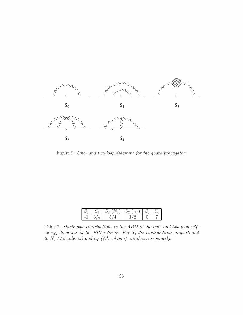
S0 S1 S2

S3 S4

Figure 2: One- and two-loop diagrams for the quark propagator.

S0 S1 S2 (Nc) S2 (nf) S3 S4

-1 3/4 5/4 1/2 0 7

Table 2: Single pole contributions to the ADM of the one- and two-loop self-energy diagrams in the FRI scheme. For S2 the contributions proportionalto Nc (3rd column) and nf (4th column) are shown separately.

26

D4 D5 D6 D7 D8 D9

D10 D11 D12 D13 D14 D15

D16 D17 D18 D19 D20 D21

D22 D23 D24 D25 D26 D27

D28 D29 D30 D31

Figure 3: Two-loop Feynman diagrams.

27

states and gauge. The results in this case are the following

A+1 = 6 −

6

NcA−

1 = −6 −6

Nc

B1 =6

NcC1 = 12

D1 = 0 E1 = −6Nc +6

Nc

F+1 = 6 − 6Nc +

6

NcF−

1 = −6 − 6Nc +6

Nc

G+1 =

1

2−

1

Nc

G−1 = −

1

2−

1

Nc

H+1 = −24 −

48

Nc

H−1 = 24 −

48

Nc

I+1 = 6 + 2Nc −

2

Nc

I−1 = −6 + 2Nc −2

Nc

.

(65)

Our results agree with those obtained in ref. [2].

For the two-loop ADM we obtained (with β0λ computed from eq. (40) for

λ = 1)

A±2 = −

209

3−

57

2N2c

±39

Nc±

355Nc

6∓

32nf3

+32nf3Nc

± 3 β0λ

(1 ∓

1

Nc

)

B2 =355

6+

15

2N2c

−32nf3Nc

+3 β0

λ

Nc

C2 = −6

Nc+

418Nc

3−

64nf3

+ 6 β0λ

D2 =9

Nc−

9Nc

4

E2 =481

6+

15

2N2c

−445N2

c

6−

32nf3Nc

+32Nc nf

3+ 3 β0

λ

(1

Nc−Nc

)(66)

F±2 =

209

3−

27

2N2c

±272Nc

3−

445N2c

6∓

32nf3

−32nf3Nc

+32Nc nf

3

±3 β0λ

(1 ±

1

Nc∓Nc

)

G±2 = −

263

18−

2

N2c

±4

Nc±

59Nc

9∓

8nf9

+16nf9Nc

±1

4β0λ

(1 ∓

2

Nc

)

28

H±2 = −

1240

3−

96

N2c

±192

Nc∓

800Nc

3±

128nf3

+256nf3Nc

∓ 12 β0λ

(1 ±

2

Nc

)

I±2 = −209

9−

59

2N2c

±32

Nc

±140Nc

3+

409N2c

18∓

32nf3

+32nf9Nc

−32Nc nf

9

±β0λ

(3 ∓

1

Nc±Nc

).

For γ± (1)FRI , we have shown explicitely those terms, proportional to β0

λ, whichcancel λ∂JFRI/∂λ in eq. (30). From the one- and two-loop matrix elementsof γ±FRI , by solving eq. (30), one can easily compute JFRI . By writing JFRIas

J±FRI ≡

J±11 0 0 0 00 J22 ±J23 0 00 ±J32 J33 0 00 0 0 J±

44 J±45

0 0 0 J±54 J±

55

, (67)

we obtain

J+11 =

−(23931 − 2862nf + 128n2

f

)

6 (33 − 2nf)2

J−11 =

28089 − 3114nf + 128n2f

3 (33 − 2nf)2

J22 =−(1437345 − 221058nf + 13488n2

f − 256n3f

)

24 (33 − 2nf)2 (30 − nf )

J23 =45

16 (30 − nf)

J32 =−4347675 + 2468583nf − 294786n2

f + 14928n3f − 256n4

f

4 (30 − nf ) (3 − nf ) (33 − 2nf)2

J33 =−(−15575085 + 2142036nf − 115572n2

f + 2048n3f

)

24 (33 − 2nf)2 (30 − nf)

J+44 =

4176675 − 5048688nf + 669548n2f − 36624n3

f + 640n4f

3 (33 − 2nf)2(125 − 132nf + 4n2

f

)

J−44 =

12084435 − 14286828nf + 1744892n2f − 86016n3

f + 1408n4f

3 (33 − 2nf)2(125 − 132nf + 4n2

f

) (68)

29

J+45 =

20(−277425 − 767424nf + 118876n2

f − 7056n3f + 128n4

f

)

3 (33 − 2nf)2(125 − 132nf + 4n2

f

)

J−45 =

4(791235 + 1102188nf − 152932n2

f + 7776n3f − 128n4

f

)

3 (33 − 2nf)2(125 − 132nf + 4n2

f

)

J+54 =

−898695 + 1066800nf − 142204n2f + 7632n3

f − 128n4f

36 (33 − 2nf)2(125 − 132nf + 4n2

f

)

J−54 =

5(1208169 − 1422948nf + 169780n2

f − 8064n3f + 128n4

f

)

36 (33 − 2nf)2(125 − 132nf + 4n2

f

)

J+55 =

−11915775 + 14548416nf − 2050844n2f + 119952n3

f − 2176n4f

9 (33 − 2nf)2(125 − 132nf + 4n2

f

)

J−55 =

−957555 + 1949172nf − 126428n2f − 2016n3

f + 128n4f

9 (33 − 2nf)2(125 − 132nf + 4n2

f

) .

5.2 Relation between FRI and other renormalization

schemes

In this subsection, we give the recipe to pass from FRI to other schemeswhich may be useful for practical applications: LRI, for lattice calculations,and the standard MS NDR scheme. All we need to know is the shift matrix

JLRI = JFRI + rTFRIJMS = JFRI + rTFRI − rT

MS. (69)

From the knowledge of J in a given renormalization scheme, we can imme-diately obtain the evolution matrix W [µ,M ] using eqs. (21) and (23).

As discussed in subsec. 3.2, the renormalization scheme is completelydefined by the matrix r of eq. (53), computed for given external momentaand gauge. We choose quarks with equal momentum p as external states andthe Landau gauge. The field renormalization constant is computed in LRIaccording to eq. (60), which gives Zψ = 1. We denote as rFRI , rLRI and rMS

the three cases considered here: rLRI is obviously zero and rMS is a 20 × 20

30

matrix because this regularization (and consequently the corresponding MS-renormalization scheme) does not respect chiral and Fierz symmetries. Bydenoting with r++ the 5 × 5 sub-matrix in the Q+

i sector and similarly forr+−, r−+ and r−−, we get (see also ref. [14] for the operators Q±

1,2,3),

(r±±FRI)11 = ±

(3

2+ 12 ln 2

)−

3

2Nc−

12 ln 2

Nc

(r±±FRI)22 =

1

2Nc−

2 ln 2

Nc

(r±±FRI)23 = ± (1 − 4 ln 2)

(r±±FRI)32 = ∓

(1

2+ ln 2

)

(r±±FRI)33 =

1

2Nc−

2 ln 2

Nc−

3Nc

2(70)

(r±±FRI)44 = ±

(1

2+ 4 ln 2

)+

1

2Nc−

2 ln 2

Nc−

3Nc

2

(r±±FRI)45 = ±

(5

24+

2 ln 2

3

)−

1

6Nc−

5 ln 2

6Nc

(r±±FRI)54 = ∓ (2 − 32 ln 2) −

8

Nc

−40 ln 2

Nc

(r±±FRI)55 = ±

(7

6+

28 ln 2

3

)−

5

6Nc−

26 ln 2

3Nc+Nc

2

and

(r±±

MS)11 = ∓ (7 − 12 ln 2) +

7

Nc−

12 ln 2

Nc

(r±±

MS)22 = −

2

Nc

−2 ln 2

Nc

(r±±

MS)23 = ∓ (4 + 4 ln 2)

(r±±

MS)32 = ± (1 − ln 2)

(r±±

MS)33 = −

2

Nc

−2 ln 2

Nc

+ 4Nc

(r±±

MS)44 = ∓

(39

8− 4 ln 2

)−

9

2Nc

−2 ln 2

Nc

+ 4Nc

(r±±

MS)45 = ∓

(31

96−

2 ln 2

3

)+

17

24Nc

−5 ln 2

6Nc

+Nc

16(71)

31

(r±±

MS)54 = ±

(13

2+ 32 ln 2

)+

34

Nc−

40 ln 2

Nc− 7Nc

(r±±

MS)55 = ∓

(95

24−

28 ln 2

3

)+

7

6Nc−

26 ln 2

3Nc

(r±∓

MS)44 = ±

17

8−

1

2Nc

(r±∓

MS)45 = ±

3

32+

3

8Nc

−Nc

16

(r±∓

MS)54 = ±

21

2−

22

Nc

+ 7Nc

(r±∓

MS)55 = ∓

13

8+

1

2Nc

Acknowledgements

V.L., G.M. and I.S. acknowledge the M.U.R.S.T. and the INFN for partialsupport. L.S. acknowledges the support of Fondazione A. Della Riccia andof German Bundesministerium fur Bildung and Forschung under contract 06TM 874 and DFG Project Li 519/2-2.

References

[1] E. Gabrielli, A. Masiero and L. Silvestrini, Phys. Lett. B374 (1996) 80;F. Gabbiani, E. Gabrielli, A. Masiero and L. Silvestrini, Nuc. Phys. B477(1996) 321 and refs. therein.

[2] J.A. Bagger, K.T. Matchev and R.J. Zhang, preprint JHU-TIPAC-97011, hep-ph/9707225 and refs. therein.

[3] G. Beall, M. Bander and A. Soni, Phys. Rev. Lett. 48 (1982) 848.

[4] M. Beneke, G. Buchalla and I. Dunietz, Phys. Rev. D54 (1996) 4419and refs. therein.

[5] M. Neubert and C.T. Sachrajda, Nucl. Phys. B483 (1997) 339 and refs.therein.

32

[6] G. Altarelli, G. Curci, G Martinelli and S. Petrarca, Nucl. Phys. B187(1981) 461.

[7] A.J. Buras, P.H. Weisz, Nucl. Phys. B333 (1990) 66.

[8] A.J. Buras, M. Jamin and P.H. Weisz, Nucl. Phys. B347 (1990) 491.

[9] S. Herrlich and U. Nierste, Nucl. Phys. B419 (1994) 292; Phys. Rev.D52 (1995) 6505; Nucl. Phys. B476 (1996) 27.

[10] J. Urban, F. Krauss, U. Jentschura and G. Soff, HEPPH-9710245, hep-ph/9710245.

[11] A.J. Buras, M. Jamin, M.E. Lautenbacher and P.H. Weisz, Nucl. Phys.B370 (1992) 69; Addendum, Nucl. Phys. B375 (1992) 501.

[12] A.J. Buras, M. Jamin, M.E. Lautenbacher and P.H. Weisz, Nucl. Phys.B400 (1993) 37; A.J. Buras, M. Jamin and M.E. Lautenbacher,Nucl. Phys. B400 (1993) 75.

[13] M. Ciuchini, E. Franco, G. Martinelli and L. Reina, Nucl. Phys. B415(1994) 403.

[14] M. Ciuchini et al., Z. Phys. C68 (1995) 239.

[15] G. Martinelli et al., Nucl. Phys. B445 (1995) 81.

[16] A. Donini et al., Phys. Lett. B360 (1996) 83; M. Crisafulli et al.,Phys. Lett. B369 (1996) 325; A. Donini et al., Nucl. Phys. B(Proc.Suppl.)53 (1997) 883; M. Talevi, talk presented at the Workshop“Lattice QCD and Parallel Computers”, Tsukuba, March 1997, hep-lat/9705016.

[17] JLQCD Collaboration, S. Aoki et al., hep-lat/9705035; Nucl. Phys.B(Proc. Suppl.)53 (1997) 349.

[18] N.G. Deshpande and X.-G. He, Phys. Rev. Lett. 74 (1995) 26.

[19] R. Aleksan et al., Phys. Lett. B356 (1995) 95.

[20] P.S. Marrocchesi and N. Paver, hep-ph/9702353.

[21] A. Ali and C. Greub, preprint DESY 97-126, hep-ph/9707251.

33