Prepared for submission to JHEP

Towards the glueball spectrum from unquenched

lattice QCD.

E. Gregorya,d A. Irvingb B. Lucinic C. McNeiled A. Ragoe C. Richardsb E. Rinaldif,g

aDepartment of Physics, University of Cyprus, P.O. Box 20357 1678 Nicosia, CyprusbTheoretical Physics Division, Dept. of Mathematical Sciences, University of Liverpool, Liverpool

L69 7ZL, UKcDepartment of Physics, College of Science, Swansea University, Singleton Park, Swansea SA2

8PP, UKdBergische Universitat Wuppertal, Gaussstr. 20, D-42119 Wuppertal, GermanyeSchool of Computing & Mathematics, University of Plymouth, Plymouth, PL4 8AA, UKfSUPA, School of Physics and Astronomy, University of Edinburgh, Edinburgh EH9 3JZ, UKgKobayashi-Maskawa Institute for the Origin of Particles and the Universe (KMI), Nagoya Uni-

versity, Nagoya 464-8602, Japan

E-mail: gregory@uni-wuppertal.de, aci@liverpool.ac.uk,

b.lucini@swansea.ac.uk, mcneile@uni-wuppertal.de,

antonio.rago@plymouth.ac.uk, cmr@liverpool.ac.uk,

e.rinaldi@sms.ed.ac.uk

Abstract: We use a variational technique to study heavy glueballs on gauge configura-

tions generated with 2+1 flavours of ASQTAD improved staggered fermions. The varia-

tional technique includes glueball scattering states. The measurements were made using

2150 configurations at 0.092 fm with a pion mass of 360 MeV. We report masses for 10

glueball states. We discuss the prospects for unquenched lattice QCD calculations of the

oddballs.

arX

iv:1

208.

1858

v2 [

hep-

lat]

5 N

ov 2

012

Contents

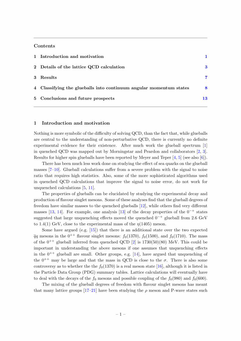
1 Introduction and motivation 1

2 Details of the lattice QCD calculation 3

3 Results 7

4 Classifying the glueballs into continuum angular momentum states 8

5 Conclusions and future prospects 13

1 Introduction and motivation

Nothing is more symbolic of the difficulty of solving QCD, than the fact that, while glueballs

are central to the understanding of non-perturbative QCD, there is currently no definite

experimental evidence for their existence. After much work the glueball spectrum [1]

in quenched QCD was mapped out by Morningstar and Peardon and collaborators [2, 3].

Results for higher spin glueballs have been reported by Meyer and Teper [4, 5] (see also [6]).

There has been much less work done on studying the effect of sea quarks on the glueball

masses [7–10]. Glueball calculations suffer from a severe problem with the signal to noise

ratio that requires high statistics. Also, some of the more sophisticated algorithms used

in quenched QCD calculations that improve the signal to noise error, do not work for

unquenched calculations [5, 11].

The properties of glueballs can be elucidated by studying the experimental decay and

production of flavour singlet mesons. Some of these analyses find that the glueball degrees of

freedom have similar masses to the quenched glueballs [12], while others find very different

masses [13, 14]. For example, one analysis [13] of the decay properties of the 0−+ states

suggested that large unquenching effects moved the quenched 0−+ glueball from 2.6 GeV

to 1.4(1) GeV, close to the experimental mass of the η(1405) meson.

Some have argued (e.g. [15]) that there is an additional state over the two expected

qq mesons in the 0++ flavour singlet mesons: f0(1370), f0(1500), and f0(1710). The mass

of the 0++ glueball inferred from quenched QCD [2] is 1730(50)(80) MeV. This could be

important in understanding the above mesons if one assumes that unquenching effects

in the 0++ glueball are small. Other groups, e.g. [14], have argued that unquenching of

the 0++ may be large and that the mass in QCD is close to the σ. There is also some

controversy as to whether the the f0(1370) is a real meson state [16], although it is listed in

the Particle Data Group (PDG) summary tables. Lattice calculations will eventually have

to deal with the decays of the f0 mesons and possible coupling of the f0(980) and f0(600).

The mixing of the glueball degrees of freedom with flavour singlet mesons has meant

that many lattice groups [17–21] have been studying the ρ meson and P-wave states such

– 1 –

as the a1(1260), b1(1235) meson using a variety of techniques so as to understand how to

deal with resonances in lattice QCD calculations.

So, in summary, there are no hadrons where glueball degrees of freedom have been con-

firmed. Looking to the future, there are ongoing experiments that are searching for glueball

degrees of freedom, such as the BES III experiment [22]. The BES III experiment has pre-

liminary [23] results for two new states with masses close to the 0+− and 1+− quenched

glueball masses. In 2018, the PANDA experiment [24] will search for heavy glueballs with

masses under 5.4 GeV. In particular they will look for oddball glueballs with exotic JPC

quantum numbers (0+−, 2+−, 1−+, 0−− and 3−+) which are not allowed in quark models

for quark-antiquark mesons. In a quenched QCD calculation, Morningstar and Peardon [2]

found two glueballs with exotic JPC = 2+− and 0+− with masses 4140(50)(200) MeV and

4740(70)(230) MeV respectively. As we review later, other quenched glueball studies have

not seen these states [25].

One motivation for studying glueballs heavier than 3 GeV is that there could be reduced

mixing with flavour singlet quark states. There have been speculations that there are no

further, or a reduced number of, light meson states above 3.1 GeV [26, 27], based on string

breaking of the heavy quark potential. Swanson [28] critiques the use of screened potentials

in hadron spectroscopy. The heaviest light meson in the PDG summary table [29] is the

f6(2510) with a mass of 2.469 GeV. It is possible that there may be no experiments capable

of producing light mesons beyond 2.5 GeV. It could be that heavier mesons made from light

quarks have large widths, so it becomes difficult to extract the masses from experiment.

Even though the signal to noise ratio is worse for heavier glueballs than for light glueballs, it

would simplify lattice QCD calculations if heavier glueballs do not mix with quark degrees

of freedom, because it would be simpler to identify a pure glueball state. For glueball masses

above 3 GeV, there is the possibility that the glueballs may mix with charmonium states.

However, Page [27] suggests that the mixing between charmonium states and glueballs will

be small, because the charm quark is heavy and hence it is difficult to excite a charm loop.

The hadron spectrum collaboration [30] has computed the spectrum of excited mesons

and baryons, although typically at a single lattice spacing and heavy quark masses. They

don’t report any meson masses above 2.8 GeV. Studying such masses is already an impres-

sive achievement, and it is not clear whether they can investigate the meson spectrum at

even higher masses.

Hagedorn conjectured that the density of light hadrons goes like em/T where m is the

mass of the light hadrons and T is a constant [31, 32]. Cohen and Krejcirik have recently

reviewed [33] the evidence that the number of light hadrons agrees with the Hagedorn

conjecture.

There may be indirect ways of determining whether there exist light mesons in the

regime 3 to 6 Gev, using information from thermodynamic studies. For example, the hadron

resonance gas model (HRGM) is used in the phenomenology of heavy ion experiments

and has successfully reproduced some results from lattice QCD calculations at non-zero

temperature. The HRGM depends on the number of mesons and baryon states. Typically

the meson and baryon states listed in the PDG are used, however Chatterjee et al. [34]

have studied a different density of states, with mesons with masses higher than those listed

– 2 –

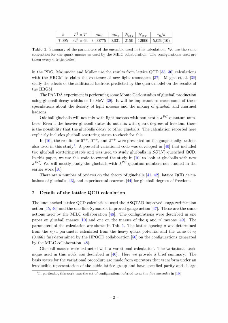
β L3 × T aml ams Ncfg Ntraj r0/a

7.095 323 × 64 0.00775 0.031 2150 12900 5.059(10)

Table 1. Summary of the parameters of the ensemble used in this calculation. We use the same

convention for the quark masses as used by the MILC collaboration. The configurations used are

taken every 6 trajectories.

in the PDG. Majumder and Muller use the results from lattice QCD [35, 36] calculations

with the HRGM to claim the existence of new light resonances [37]. Megias et al. [38]

study the effects of the additional hadrons predicted by the quark model on the results of

the HRGM.

The PANDA experiment is performing some Monte Carlo studies of glueball production

using glueball decay widths of 10 MeV [39]. It will be important to check some of these

speculations about the density of light mesons and the mixing of glueball and charmed

hadrons.

Oddball glueballs will not mix with light mesons with non-exotic JPC quantum num-

bers. Even if the heavier glueball states do not mix with quark degrees of freedom, there

is the possibility that the glueballs decay to other glueballs. The calculation reported here

explicitly includes glueball scattering states to check for this.

In [10], the results for 0++, 0−+, and 2++ were presented on the gauge configurations

also used in this study1. A powerful variational code was developed in [40] that included

two glueball scattering states and was used to study glueballs in SU(N) quenched QCD.

In this paper, we use this code to extend the study in [10] to look at glueballs with new

JPC . We will mostly study the glueballs with JPC quantum numbers not studied in the

earlier work [10].

There are a number of reviews on the theory of glueballs [41, 42], lattice QCD calcu-

lations of glueballs [43], and experimental searches [44] for glueball degrees of freedom.

2 Details of the lattice QCD calculation

The unquenched lattice QCD calculations used the ASQTAD improved staggered fermion

action [45, 46] and the one link Symanzik improved gauge action [47]. These are the same

actions used by the MILC collaboration [48]. The configurations were described in one

paper on glueball masses [10] and one on the masses of the η and η′ mesons [49]. The

parameters of the calculation are shown in Tab. 1. The lattice spacing a was determined

from the r0/a parameter calculated from the heavy quark potential and the value of r0(0.4661 fm) determined by the HPQCD collaboration [50] on the configurations generated

by the MILC collaboration [48].

Glueball masses were extracted with a variational calculation. The variational tech-

nique used in this work was described in [40]. Here we provide a brief summary. The

basis states for the variational procedure are made from operators that transform under an

irreducible representation of the cubic lattice group and have specified parity and charge

1In particular, this work uses the set of configurations referred to as the fine ensemble in [10].

– 3 –

conjugation quantum numbers. The irreducible representations of the cubic group, which

is the discrete rotational symmetry group of the lattice, are conventionally called A1, A2,

E, T1 and T2. Representations A1 and A2 have dimension 1, E has dimension 2 and T1 and

T2 have dimension 3. Below, we show how the continuum spin can be obtained from mass

eigenstates transforming according to an irreducible representation of the cubic group.

On a given timeslice, a single glueball operator with well-defined rotational quan-

tum number is a prescribed linear combination of traced Wilson loops of a given shape.

Eigenstates of parity are obtained by considering the starting linear combination and the

reflected one, while eigenstates of charge conjugations are given by the real part (C = 1)

and the imaginary part (C = −1) of that combination. In our calculations, we considered

operators containing shapes from length 4 to length 10. In addition to single glueball oper-

ators, the basis states include two-glueball scattering states (which involve products of two

basic shapes) and bi-torelon operators (products of two loops winding in a compact spatial

direction; note that these operators are not necessarily straight lines). In order to keep the

number of operators under control, we limited the number of single glueball operators to at

most 30. The shapes we included in our calculations are those that contribute in as many

channels as possible and, barring shapes that for symmetry reasons do not contribute to

given channels, the same basis shapes have been used for all the quantum number assign-

ments. Other constraints imposed on the basis operators were that the variational basis

must contain shapes of all lengths and that a given shape can contribute at most once in a

given channel. This allowed us to include a broad range of shapes and lengths in our basis.

A Mathematica program systematically constructed the basis operators with the requested

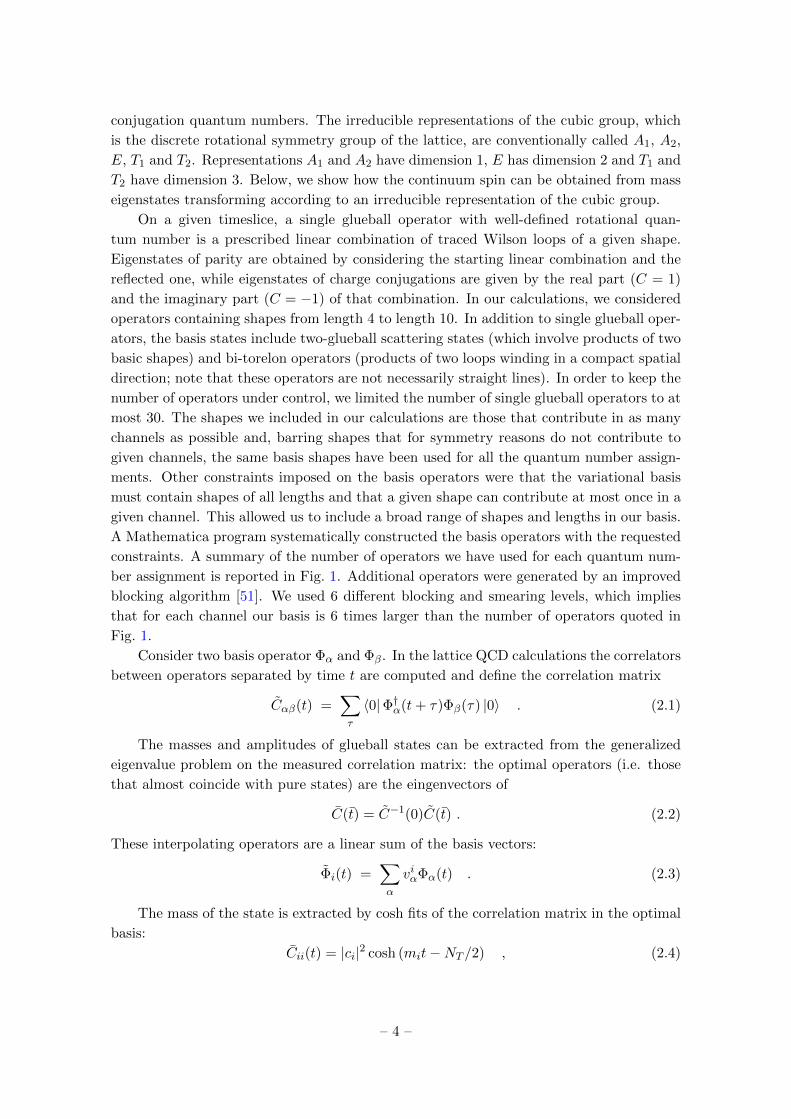
constraints. A summary of the number of operators we have used for each quantum num-

ber assignment is reported in Fig. 1. Additional operators were generated by an improved

blocking algorithm [51]. We used 6 different blocking and smearing levels, which implies

that for each channel our basis is 6 times larger than the number of operators quoted in

Fig. 1.

Consider two basis operator Φα and Φβ. In the lattice QCD calculations the correlators

between operators separated by time t are computed and define the correlation matrix

Cαβ(t) =∑τ

〈0|Φ†α(t+ τ)Φβ(τ) |0〉 . (2.1)

The masses and amplitudes of glueball states can be extracted from the generalized

eigenvalue problem on the measured correlation matrix: the optimal operators (i.e. those

that almost coincide with pure states) are the eingenvectors of

C(t) = C−1(0)C(t) . (2.2)

These interpolating operators are a linear sum of the basis vectors:

Φi(t) =∑α

viαΦα(t) . (2.3)

The mass of the state is extracted by cosh fits of the correlation matrix in the optimal

basis:

Cii(t) = |ci|2 cosh (mit−NT /2) , (2.4)

– 4 –

A1

++A

1

+-A

1

-+A

1

--A

2

++A

2

+-A

2

-+A

2

--E

++E

+-E

-+E

--T

1

++T

1

+-T

1

-+T

1

--T

2

++T

2

+-T

2

-+T

2

--0

10

20

30

40

Num

ber

of opera

tors

GlueballScattering

Bi-torelon

Figure 1. Number of basis operators (before blocking and smearing) in each channel, for single

glueballs, scattering states and bi-torelon states.

where NT is the length of the lattice in the time direction and the cosh functional form is

a consequence of the usual exponential decay in a lattice with periodic boundary condition

in the time direction.

In general, glueball correlators are very noisy and this limits the usefulness of numerical

correlators to short time separations. However, although Eq. (2.4) is only valid at large

t, if the overlap with an Hamiltonian state is almost perfect, it is possible to extract a

reliable value for the mass at short time separation, since the decay is largely dominated

by a single state. For this to be true, a careful construction of the variational basis is

paramount. Whether an optimal state Φi is a good approximation of the Hamiltonian

eigenstates can be checked by looking at the value of the overlap |ci|2: the closer this number

is to one from below (with one being the unitarity limit), the better is the variational

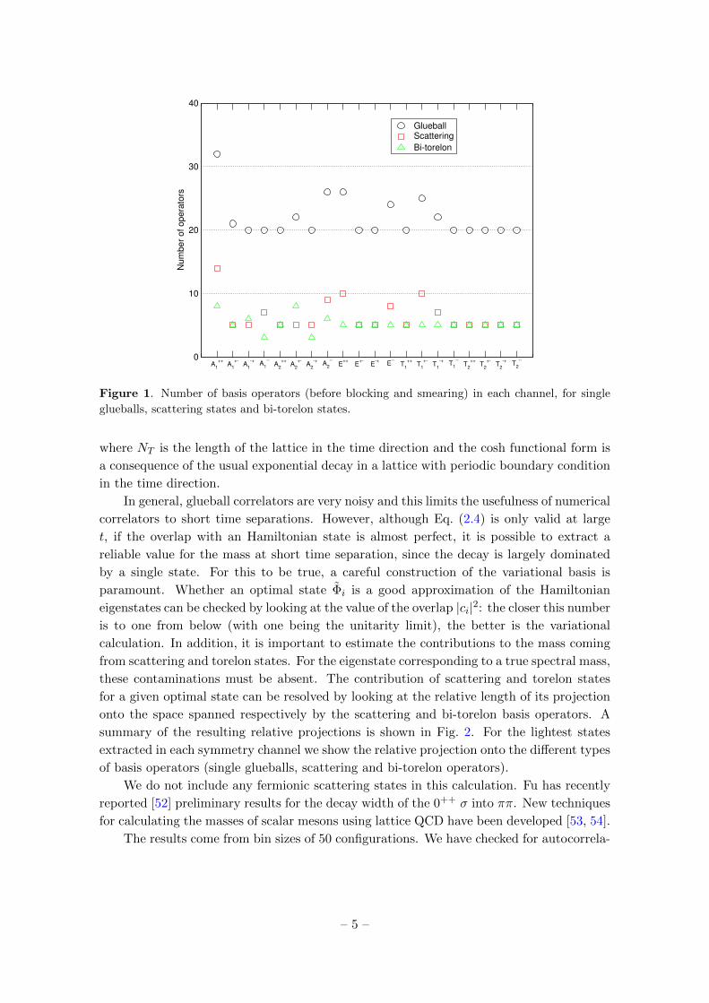
calculation. In addition, it is important to estimate the contributions to the mass coming

from scattering and torelon states. For the eigenstate corresponding to a true spectral mass,

these contaminations must be absent. The contribution of scattering and torelon states

for a given optimal state can be resolved by looking at the relative length of its projection

onto the space spanned respectively by the scattering and bi-torelon basis operators. A

summary of the resulting relative projections is shown in Fig. 2. For the lightest states

extracted in each symmetry channel we show the relative projection onto the different types

of basis operators (single glueballs, scattering and bi-torelon operators).

We do not include any fermionic scattering states in this calculation. Fu has recently

reported [52] preliminary results for the decay width of the 0++ σ into ππ. New techniques

for calculating the masses of scalar mesons using lattice QCD have been developed [53, 54].

The results come from bin sizes of 50 configurations. We have checked for autocorrela-

– 5 –

A1

++A

1

+-A

1

-+A

1

--A

2

++A

2

+-A

2

-+A

2

--E

++E

+-E

-+E

--T

1

++T

1

+-T

1

-+T

1

--T

2

++T

2

+-T

2

-+T

2

--0

20

40

60

80

100

Re

lative

pro

jectio

ns [

%]

GlueballsScattering

Bi-torelon

Figure 2. Summary of the projections relative to the subspace spanned by different types of basis

operators for the lightest states in the spectrum.

0 2 4 6 8t/a

0.0001

0.001

0.01

0.1

1

C(t

)/C

(0)

ground state

first excitation

A1

++

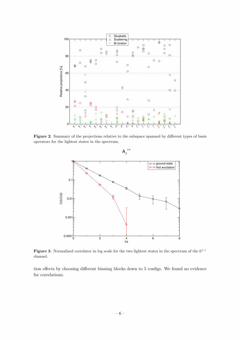
Figure 3. Normalized correlator in log scale for the two lightest states in the spectrum of the 0++

channel.

tion effects by choosing different binning blocks down to 5 configs. We found no evidence

for correlations.

– 6 –

0 2 4 6 8t/a

0

0.5

1

1.5

2

am

eff

am = 0.839(28) |c0|2 = 0.94

am = 1.447(55) |c0|2 = 0.98

Figure 4. Effective mass plateaux for ground state (circles) and the first excitation (squares) in the

0++ channel. The fitted values are shown with solid lines (the dashed lines represent one standard

deviation).

0 1 2 3 4 5t/a

0.001

0.01

0.1

1

C(t

)/C

(0)

ground state

ground state

E++

Figure 5. Normalized correlator in log scale for the lightest state in the spectrum of the E++

channel.

3 Results

We reduced the variational correlators Eq. (2.1) truncating the diagonal matrix Eq. (2.2) to

the 5 highest eigenvalues (corresponding to the 5 lowest masses). The diagonal correlators

– 7 –

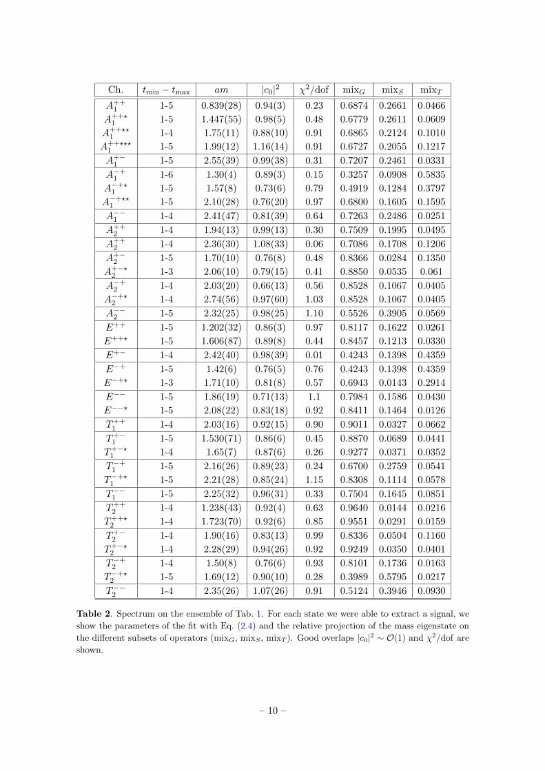
are fitted to the fit model in Eq. (2.4). The functional form is a good approximation if the

overlap |ci|2 ∼ O(1) and the χ2/dof ∼ O(1). All the states we were able to measure have

0.65 < |ci|2 < 1.1, with order 0.1 errors and 0 < χ2/dof < 1.25.

The correlator for the lightest glueball (the A++1 channel, which in the continuum

encodes the scalar 0++ glueball) and its first excitation is shown in Fig. 3 on a logarithmic

scale. The effective mass plateaux of these two states with the corresponding estimate of

the fitted masses from the fit in Eq. (2.4) are reported in Fig. 4. A similar plot for the E++

channel corresponding to the continuum tensor glueball is shown in Fig. 5. For the A++1 , we

have investigated alternative variational calculations that include only some of the subsets

of our operators (only single glueball operators or only scattering and torellon operators).

We note that in both cases the mass of the ground state is the same within errors. This

phenomenon is different from what happens in pure gauge, where for sets excluding single

glueball operators the ground state mass is roughly twice the mass of the ground state one

finds when single glueball are included in the variational basis [40]. This might be due to

the explicit breaking of centre symmetry in the presence of dynamical fermions. Although

the coupling of glueball states and single torellon states was found to be negligible in [8],

it is possible that it becomes more relevant closer to the chiral limit. To investigate this

coupling systematically would require variational calculations with a basis including single

torellon operators at various quark masses close to the chiral limit. A similar calculation

is beyond the scope of this paper.

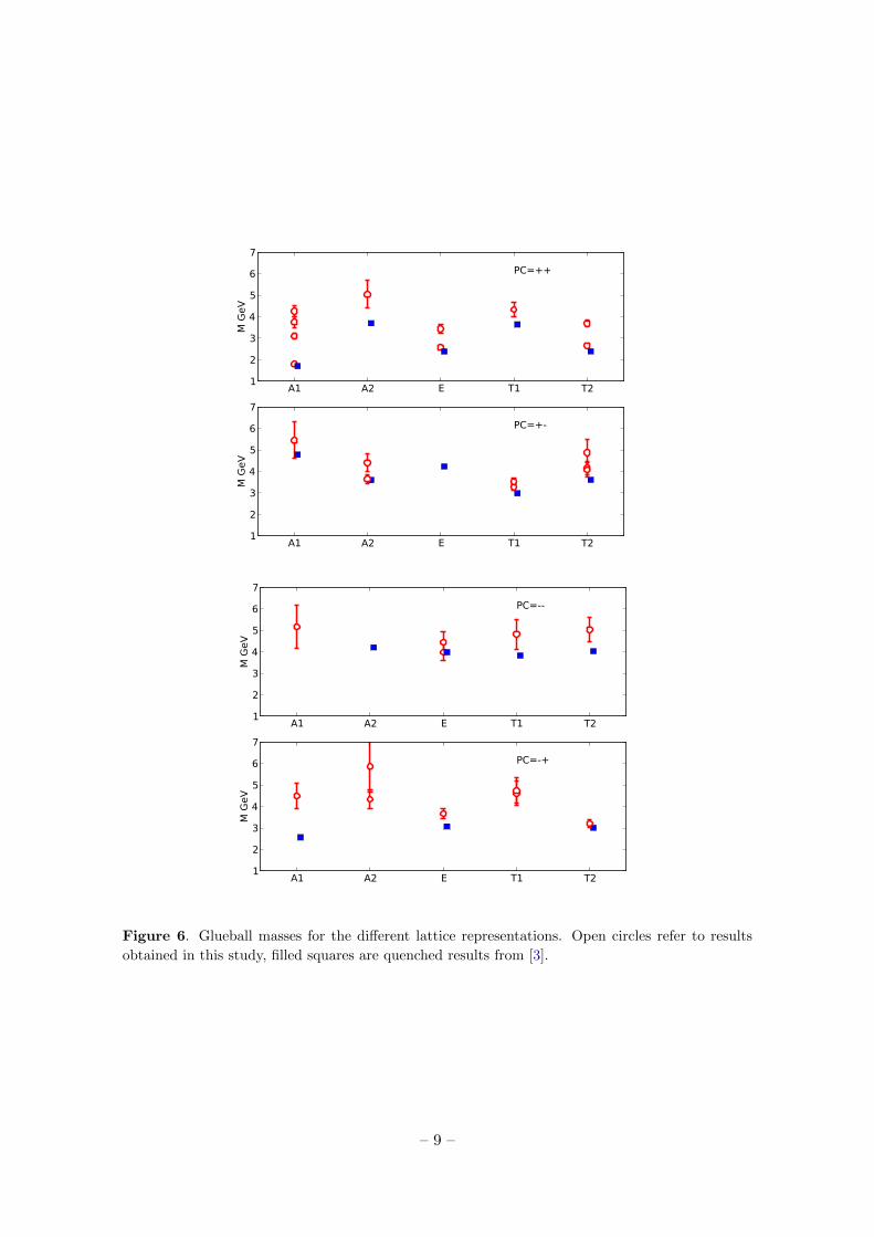
In Fig. 6 we plot the glueball masses for each lattice representation. A summary of

the spectrum is reported in Tab. 2. We define glueball states as those with an overlap of

at least 65% onto the single glueball operators.

We also include the results from Chen et al. [3] from a quenched lattice QCD calculation in

the continuum limit. Fig. 6 does not show any significant unquenching effects, although the

continuum limit of the unquenched results should be taken before a definitive statement

can be made.

4 Classifying the glueballs into continuum angular momentum states

Each of the states comes from an operator that is a linear combination of ones in the

variational basis. The projection on the 3 subsets can be used to identify single glueball

states from scattering or bi-torelon states. Only the A−−2 , T−+2 and T−−2 channels had

O(40)% overlap with the scattering subset of operators. Also only the A−+1 and E+−

channels had contaminations of O(40)% overlap with bi-torelons. We find that the channels

A++1 , A+−

1 , A−−1 and T−+1 had contaminations with scattering states of between 20% and

40%. The A−+1 and E−+ channels had bi-torelons contaminations between 20% and 40%.

Identification of the spin of glueball states on the lattice is non-trivial. Continuum spin

representations break down into lattice representations at finite lattic spacing. In Tab. 3

the continuum spin representations are broken down into lattice representations.

– 8 –

A1 A2 E T1 T21

2

3

4

5

6

7M

GeV

PC=++

A1 A2 E T1 T21

2

3

4

5

6

7

M G

eV

PC=+-

A1 A2 E T1 T21

2

3

4

5

6

7

M G

eV

PC=--

A1 A2 E T1 T21

2

3

4

5

6

7

M G

eV

PC=-+

Figure 6. Glueball masses for the different lattice representations. Open circles refer to results

obtained in this study, filled squares are quenched results from [3].

– 9 –

Ch. tmin − tmax am |c0|2 χ2/dof mixG mixS mixT

A++1 1-5 0.839(28) 0.94(3) 0.23 0.6874 0.2661 0.0466

A++?1 1-5 1.447(55) 0.98(5) 0.48 0.6779 0.2611 0.0609

A++??1 1-4 1.75(11) 0.88(10) 0.91 0.6865 0.2124 0.1010

A++???1 1-5 1.99(12) 1.16(14) 0.91 0.6727 0.2055 0.1217

A+−1 1-5 2.55(39) 0.99(38) 0.31 0.7207 0.2461 0.0331

A−+1 1-6 1.30(4) 0.89(3) 0.15 0.3257 0.0908 0.5835

A−+?1 1-5 1.57(8) 0.73(6) 0.79 0.4919 0.1284 0.3797

A−+??1 1-5 2.10(28) 0.76(20) 0.97 0.6800 0.1605 0.1595

A−−1 1-4 2.41(47) 0.81(39) 0.64 0.7263 0.2486 0.0251

A++2 1-4 1.94(13) 0.99(13) 0.30 0.7509 0.1995 0.0495

A++2 1-4 2.36(30) 1.08(33) 0.06 0.7086 0.1708 0.1206

A+−2 1-5 1.70(10) 0.76(8) 0.48 0.8366 0.0284 0.1350

A+−?2 1-3 2.06(10) 0.79(15) 0.41 0.8850 0.0535 0.061

A−+2 1-4 2.03(20) 0.66(13) 0.56 0.8528 0.1067 0.0405

A−+?2 1-4 2.74(56) 0.97(60) 1.03 0.8528 0.1067 0.0405

A−−2 1-5 2.32(25) 0.98(25) 1.10 0.5526 0.3905 0.0569

E++ 1-5 1.202(32) 0.86(3) 0.97 0.8117 0.1622 0.0261

E++? 1-5 1.606(87) 0.89(8) 0.44 0.8457 0.1213 0.0330

E+− 1-4 2.42(40) 0.98(39) 0.01 0.4243 0.1398 0.4359

E−+ 1-5 1.42(6) 0.76(5) 0.76 0.4243 0.1398 0.4359

E−+? 1-3 1.71(10) 0.81(8) 0.57 0.6943 0.0143 0.2914

E−− 1-5 1.86(19) 0.71(13) 1.1 0.7984 0.1586 0.0430

E−−? 1-5 2.08(22) 0.83(18) 0.92 0.8411 0.1464 0.0126

T++1 1-4 2.03(16) 0.92(15) 0.90 0.9011 0.0327 0.0662

T+−1 1-5 1.530(71) 0.86(6) 0.45 0.8870 0.0689 0.0441

T+−?1 1-4 1.65(7) 0.87(6) 0.26 0.9277 0.0371 0.0352

T−+1 1-5 2.16(26) 0.89(23) 0.24 0.6700 0.2759 0.0541

T−+?1 1-5 2.21(28) 0.85(24) 1.15 0.8308 0.1114 0.0578

T−−1 1-5 2.25(32) 0.96(31) 0.33 0.7504 0.1645 0.0851

T++2 1-4 1.238(43) 0.92(4) 0.63 0.9640 0.0144 0.0216

T++?2 1-4 1.723(70) 0.92(6) 0.85 0.9551 0.0291 0.0159

T+−2 1-4 1.90(16) 0.83(13) 0.99 0.8336 0.0504 0.1160

T+−?2 1-4 2.28(29) 0.94(26) 0.92 0.9249 0.0350 0.0401

T−+2 1-4 1.50(8) 0.76(6) 0.93 0.8101 0.1736 0.0163

T−+?2 1-5 1.69(12) 0.90(10) 0.28 0.3989 0.5795 0.0217

T−−2 1-4 2.35(26) 1.07(26) 0.91 0.5124 0.3946 0.0930

Table 2. Spectrum on the ensemble of Tab. 1. For each state we were able to extract a signal, we

show the parameters of the fit with Eq. (2.4) and the relative projection of the mass eigenstate on

the different subsets of operators (mixG, mixS , mixT ). Good overlaps |c0|2 ∼ O(1) and χ2/dof are

shown.

– 10 –

J A1 A2 E T1 T2

0 1 0 0 0 0

1 0 0 0 1 0

2 0 0 1 0 1

3 0 1 0 1 1

4 1 0 1 1 1

Table 3. Subduced representations J ↓ GO of the octahedral group up to J = 4. This table

illustrates the spin content of the irreducible representations of GO in terms of the continuum J .

JPC Mass MeV

Unquenched Quenched

This work M&P Ky Meyer

0−+ 2590(40)(130) 2560(35)(120) 2250(60)(100)

2−+ 3460(320) 3100(30)(150) 3040(40)(150) 2780(50)(130)

0−+ 4490(590) 3640(60)(180) 3370(150)(150)

2−+ 3480(140)(160)

5−+ 3942(160)(180)

0−− (exotic) 5166(1000)

1−− 3850(50)(190) 3830(40)(190) 3240(330)(150)

2−− 4590(740) 3930(40)(190) 4010(45)(200) 3660(130)(170)

2−− 3.740(200)(170)

3−− 4130(90)(200) 4200(45)(200) 4330(260)(200)

1+− 3270(340) 2940(30)(140) 2980(30)(140) 2670(65)(120)

3+− 3850(350) 3550(40)(170) 3600(40)(170) 3270(90)(150)

3+− 3630(140)(160)

2+− (exotic) 4140(50)(200) 4230(50)(200)

0+− (exotic) 5450(830) 4740(70)(230) 4780(60)(230)

5+− 4110(170)(190)

0++ 1795(60) 1730(50)(80) 1710(50)(80) 1475(30)(65)

2++ 2620(50) 2400(25)(120) 2390(30)(120) 2150(30)(100)

0++ 3760(240) 2670(180)(130) 2755(30)(120)

3++ 3690(40)(180) 3670(50)(180) 3385(90)(150)

0++ 3370(100)(150)

0++ 3990(210)(180)

2++ 2880(100)(130)

4++ 3640(90)(160)

6++ 4360(260)(200)

Table 4. Glueball masses with JPC assignments. The column M&P reports results from Morn-

ingstar and Peardon [2] from quenched QCD. The column labelled Ky is the data from Chen et

al. [3]. Meyer’s results are from [25].

– 11 –

Meyer and Teper [25, 55] have developed systematic techniques to classify glueball

masses into spins. Dudek et al. [56] have stressed the importance of correctly identifying

lattice representations with spin in the charmonium system. Here, we use the simplest

spin identification. We identity the J = 0 state with the A1, and J = 1 state with the T1representation, and J = 2 states with almost degenerate T2 and E representations. For

J = 2 and J = 3 states we take a weighted average of the masses in the component lattice

representations.

Morningstar and Peardon [2] found glueball states with 0−+ (ground and excited), and

2−+ quantum numbers. In the PC = −+ sector in Fig. 6 there are two almost degenerate

levels in the E and T2 representations that could come from a J = 2 state. There is one

level in the A1 representation which is relatively isolated and so is expected to couple to

0−+ states. There are also degenerate levels in the A2, and T1 representations that could

be 3−+. This would be interesting, because 3−+ is an exotic quantum number, however,

because there is no signal in T2 representation, this state is not included in the summary

tables.

In the PC = −− sector in Fig. 6, the errors are large because the masses are very

heavy. Morningstar and Peardon [2] found glueball states with 1−−, 2−−, and 3−−. Here

we see evidence for a 2−− state with near-degenerate masses in the E and T2 channel. The

results in Fig. 6 are not consistent with 3−−, because there is no signal in the A2 channel.

There is also a hint of a signal for the spin exotic 0−− state in the A1 representation, but

unfortunately with large errors.

For the operators with PC = ++ in Fig. 6, there is potentially a rich mixture of

states. Morningstar and Peardon [2] found glueball states with 0++ (ground and excited),

and 2++. There are two 0++ states in the A1 channel. There are two almost degenerate

states in the E and T2 channel that would correspond to a 2++ state in the continuum.

The agreement of the effective masses for these two lattice states, together with the fitted

masses using Eq. (2.4) is shown in Fig. 7. The mass degeneracy between these two channels

is supposed to be exact in the continuum limit, when the full three-dimensional rotational

symmetry is dynamically restored.

There is potentially a 4++ appearing in the A1, E, T1, and T2 representations. There

is also a potential 3++ state in the A2 representation, but there is no hint of degenerate

states in the T1 and T2 representations.

In quenched QCD, Morningstar and Peardon [2] found glueball states with JPC =

3+−, 1+−, 2+−, and 0+−. The summary of the masses in Fig. 6 doesn’t show a signal in

the E+−, so our results are inconsistent with an exotic 2+− state. There is evidence for

states with JPC = 3+−, 1+−, and 0+−.

In Tab. 4 we summarise our assignments for JPC quantum numbers to the glueball

masses from operators, and compare with other results in the literature from quenched

QCD calculations. Note that the calculations by Meyer and Teper [25, 55] used the string

tension to determine the lattice spacing, however Morningstar and Peardon [2] and Chen

et al. [3] used r0. This may cause a systematic difference in the results. Meyer [57] showed

that consistent results were obtained for the masses of the tensor and scalar glueballs from

the different glueball calculations [2, 3, 25, 55], if r0 was always used to determine the

– 12 –

0 1 2 3 4 5t/a

0

0.5

1

1.5

2

am

eff

E++

T2

++

amE

++ = 1.202(32)

amT

2

++ = 1.238(43)

Figure 7. The ground state effective mass in the E++ channel is compared to the one in the T++2

channel. These channels correspond to the continuum spin J = 2 representation and are supposed

to be degenerate when the complete rotational symmetry is restored.

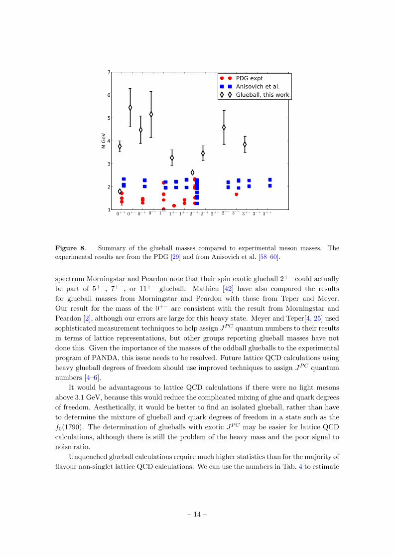
lattice spacing. In Fig. 8 we plot the summary of the glueball masses.

To compare with experiment we use the masses in the PDG. However we also include

the additional masses reported by the Crystal Barrel collaboration, reviewed by Bugg [61].

Note that the Crystal Barrel experiment could only find new states in a restricted mass

range. As explained in [60], some of the results from Anisovich et al. [58–60] are not

included in the PDG summary tables, because they are neither confirmed nor excluded

by other experiments. We plot the results for I = 0 mesons in [58, 59], but plot the 2++

states from [60]. These additional meson states from Anisovich et al. [58–60] have been

used to find some experimental glueball candidates [62] from the quenched calculations of

Morningstar and Peardon.

Bali [63] has plotted the quenched glueball spectrum with the experimental masses of

the charmonium system.

5 Conclusions and future prospects

The most conservative interpretation of our results is that the masses in terms of lattice

representations are broadly consistent with results from quenched QCD. We do not see any

evidence for large unquenching effects, however a definitive calculation requires a continuum

extrapolation, and the inclusion of fermionic operators. In Tab. 8 we tentatively assign JPC

quantum numbers to 10 glueballs.

Of particular note in Tab. 4 is that Meyer and Teper [25] do not see the two spin

exotic states identified by Morningstar and Peardon [2]. In their summary of the glueball

– 13 –

0+ + 0+− 0−+ 0−− 1−− 1+− 1+ + 2+ + 2−+ 2+− 2−− 3−− 3+− 3−+ 3+ +1

2

3

4

5

6

7

M G

eV

PDG exptAnisovich et al.Glueball, this work

Figure 8. Summary of the glueball masses compared to experimental meson masses. The

experimental results are from the PDG [29] and from Anisovich et al. [58–60].

spectrum Morningstar and Peardon note that their spin exotic glueball 2+− could actually

be part of 5+−, 7+−, or 11+− glueball. Mathieu [42] have also compared the results

for glueball masses from Morningstar and Peardon with those from Teper and Meyer.

Our result for the mass of the 0+− are consistent with the result from Morningstar and

Peardon [2], although our errors are large for this heavy state. Meyer and Teper[4, 25] used

sophisticated measurement techniques to help assign JPC quantum numbers to their results

in terms of lattice representations, but other groups reporting glueball masses have not

done this. Given the importance of the masses of the oddball glueballs to the experimental

program of PANDA, this issue needs to be resolved. Future lattice QCD calculations using

heavy glueball degrees of freedom should use improved techniques to assign JPC quantum

numbers [4–6].

It would be advantageous to lattice QCD calculations if there were no light mesons

above 3.1 GeV, because this would reduce the complicated mixing of glue and quark degrees

of freedom. Aesthetically, it would be better to find an isolated glueball, rather than have

to determine the mixture of glueball and quark degrees of freedom in a state such as the

f0(1790). The determination of glueballs with exotic JPC may be easier for lattice QCD

calculations, although there is still the problem of the heavy mass and the poor signal to

noise ratio.

Unquenched glueball calculations require much higher statistics than for the majority of

flavour non-singlet lattice QCD calculations. We can use the numbers in Tab. 4 to estimate

– 14 –

roughly the number of configurations required to achieve a given accuracy. The most

interesting states in Tab. 4 are the ones with exotic JPC = 0+− and 2+− quantum numbers.

Using simple 1/√Nconfigs scaling, we can estimate that we need 550,000 configurations

to get 50 MeV errors for the spin exotic 0+− glueball.

The MILC collaboration has reported time estimates to produce ensembles of gauge

configurations with 2+1+1 flavours of sea quarks with the HISQ improved staggered action.

With the light quark a tenth of the strange quark mass, they estimate the time to generate

1000 configurations as 35, 128, and 352 Million core hours for the lattice spacings of: 0.09,

0.06, and 0.045 fm respectively2. These numbers suggest that it is still too expensive to

reduce the errors on the masses of the oddball glueballs. Lattice QCD calculations that

use anisotropic lattices may be computationally cheaper.

The heavy glueballs may mix with charmonium states. To study this type of mixing

will probably require both charm loops in the sea and the computation of disconnected

diagrams [64, 65] for the charmonium valence states. There are a number of lattice QCD

calculations, such as the one by the MILC collaboration [66], that include the dynamics of

the charm quarks in the sea.

It is an exciting time for lattice QCD, with some unquenched lattice QCD calculations

done with physical quark masses, and many unquenched calculations resulting in errors at

the O(1%) level. The progress on lattice QCD calculations of glueballs is slower. However,

the start of the PANDA experiment in 2018 provides an important deadline for lattice

QCD calculations of glueballs.

Acknowledgments

The calculations were performed on the Liverpool cluster that is part of DiRAC funded by

STFC. The gauge configurations were generated on the QCDOC [67]. We used Chroma [68]

to make fermionic measurements. The work of B.L. is supported by the Royal Society and

by STFC. ER is supported by a SUPA prize studentship and a JSPS short-term fellowship.

References

[1] UKQCD Collaboration, G. Bali et al., A Comprehensive lattice study of SU(3) glueballs,

Phys.Lett. B309 (1993) 378–384, [hep-lat/9304012].

[2] C. J. Morningstar and M. J. Peardon, The glueball spectrum from an anisotropic lattice

study, Phys. Rev. D60 (1999) 034509, [hep-lat/9901004].

[3] Y. Chen et al., Glueball spectrum and matrix elements on anisotropic lattices, Phys. Rev.

D73 (2006) 014516, [hep-lat/0510074].

[4] H. B. Meyer and M. J. Teper, Glueball Regge trajectories and the pomeron: A Lattice study,

Phys.Lett. B605 (2005) 344–354, [hep-ph/0409183].

[5] H. B. Meyer, The Yang-Mills spectrum from a two level algorithm, JHEP 0401 (2004) 030,

[hep-lat/0312034].

2Talk presented by Paul Mackenzie at May 2011 review of the lqcd project.

– 15 –

[6] D. Q. Liu and J. M. Wu, The First calculation for the mass of the ground 4++ glueball state

on lattice, Mod.Phys.Lett. A17 (2002) 1419–1430, [hep-lat/0105019].

[7] TXL Collaboration, G. S. Bali et al., Static potentials and glueball masses from QCD

simulations with Wilson sea quarks, Phys.Rev. D62 (2000) 054503, [hep-lat/0003012].

[8] UKQCD Collaboration, A. Hart and M. Teper, On the glueball spectrum in O(a) improved

lattice QCD, Phys.Rev. D65 (2002) 034502, [hep-lat/0108022].

[9] UKQCD Collaboration, A. Hart, C. McNeile, C. Michael, and J. Pickavance, A Lattice study

of the masses of singlet 0++ mesons, Phys.Rev. D74 (2006) 114504, [hep-lat/0608026].

[10] UKQCD Collaboration, C. M. Richards, A. C. Irving, E. B. Gregory, and C. McNeile,

Glueball mass measurements from improved staggered fermion simulations, Phys. Rev. D82

(2010) 034501, [arXiv:1005.2473].

[11] M. Della Morte and L. Giusti, A novel approach for computing glueball masses and matrix

elements in Yang-Mills theories on the lattice, JHEP 1105 (2011) 056, [arXiv:1012.2562].

[12] H.-Y. Cheng, C.-K. Chua, and K.-F. Liu, Scalar glueball, scalar quarkonia, and their mixing,

Phys. Rev. D74 (2006) 094005, [hep-ph/0607206].

[13] H.-Y. Cheng, H.-n. Li, and K.-F. Liu, Pseudoscalar glueball mass from eta - eta-prime - G

mixing, Phys.Rev. D79 (2009) 014024, [arXiv:0811.2577].

[14] G. Mennessier, S. Narison, and W. Ochs, Glueball nature of the sigma/f0(600) from pi-pi and

gamma-gamma scatterings, Phys. Lett. B665 (2008) 205–211, [arXiv:0804.4452].

[15] F. E. Close and A. Kirk, Scalar glueball q anti-q mixing above 1-GeV and implications for

lattice QCD, Eur.Phys.J. C21 (2001) 531–543, [hep-ph/0103173].

[16] W. Ochs, No indication of f0(1370) in pi pi phase shift analyses, AIP Conf. Proc. 1257

(2010) 252–256, [arXiv:1001.4486].

[17] CP-PACS Collaboration, S. Aoki et al., Lattice QCD Calculation of the rho Meson Decay

Width, Phys.Rev. D76 (2007) 094506, [arXiv:0708.3705].

[18] ETM Collaboration, K. Jansen, C. McNeile, C. Michael, and C. Urbach, Meson masses and

decay constants from unquenched lattice QCD, Phys.Rev. D80 (2009) 054510,

[arXiv:0906.4720].

[19] X. Feng, K. Jansen, and D. B. Renner, Resonance Parameters of the rho-Meson from Lattice

QCD, Phys.Rev. D83 (2011) 094505, [arXiv:1011.5288].

[20] C. Lang, D. Mohler, S. Prelovsek, and M. Vidmar, Coupled channel analysis of the rho

meson decay in lattice QCD, Phys.Rev. D84 (2011) 054503, [arXiv:1105.5636].

[21] S. Prelovsek, C. Lang, D. Mohler, and M. Vidmar, Decay of rho and a1 mesons on the lattice

using distillation, PoS LATTICE2011 (2011) 137, [arXiv:1111.0409].

[22] D. Asner, T. Barnes, J. Bian, I. Bigi, N. Brambilla, et al., Physics at BES-III,

Int.J.Mod.Phys. A24 (2009) S1–794, [arXiv:0809.1869].

[23] BESIII Collaboration, S. L. Olsen, News from BESIII, arXiv:1203.4297.

[24] PANDA Collaboration, M. Lutz et al., Physics Performance Report for PANDA: Strong

Interaction Studies with Antiprotons, arXiv:0903.3905.

[25] H. B. Meyer, Glueball Regge trajectories, hep-lat/0508002. Ph.D. Thesis.

– 16 –

[26] M. M. Brisudova, L. Burakovsky, and J. Goldman, Effective functional form of Regge

trajectories, Phys.Rev. D61 (2000) 054013, [hep-ph/9906293].

[27] P. R. Page, Multi-GeV gluonic mesons, hep-ph/0107016.

[28] E. S. Swanson, Unquenching the quark model and screened potentials, J.Phys.G G31 (2005)

845–854, [hep-ph/0504097].

[29] Particle Data Group Collaboration, K. Nakamura et al., Review of particle physics,

J.Phys.G G37 (2010) 075021.

[30] J. J. Dudek et al., Isoscalar meson spectroscopy from lattice QCD, Phys. Rev. D83 (2011)

111502, [arXiv:1102.4299].

[31] R. Hagedorn, Statistical thermodynamics of strong interactions at high-energies, Nuovo

Cim.Suppl. 3 (1965) 147–186.

[32] R. Hagedorn, Hadronic matter near the boiling point, Nuovo Cim. A56 (1968) 1027–1057.

[33] T. D. Cohen and V. Krejvcivrik, Does the empirical meson spectrum support the Hagedorn

conjecture?, arXiv:1107.2130.

[34] S. Chatterjee, R. M. Godbole, and S. Gupta, Stabilizing hadron resonance gas models, Phys.

Rev. C81 (2010) 044907, [arXiv:0906.2523].

[35] S. Borsanyi, G. Endrodi, Z. Fodor, A. Jakovac, S. D. Katz, et al., The QCD equation of state

with dynamical quarks, JHEP 1011 (2010) 077, [arXiv:1007.2580].

[36] Wuppertal-Budapest Collaboration, S. Borsanyi et al., Is there still any Tc mystery in

lattice QCD? Results with physical masses in the continuum limit III, JHEP 1009 (2010)

073, [arXiv:1005.3508].

[37] A. Majumder and B. Muller, Hadron Mass Spectrum from Lattice QCD, Phys.Rev.Lett. 105

(2010) 252002, [arXiv:1008.1747].

[38] E. Megias, E. R. Arriola, and L. Salcedo, The hadron resonance gas model: thermodynamics

of QCD and Polyakov loop, arXiv:1207.7287.

[39] U. Wiedner, Future Prospects for Hadron Physics at PANDA, Prog.Part.Nucl.Phys. 66

(2011) 477–518, [arXiv:1104.3961].

[40] B. Lucini, A. Rago, and E. Rinaldi, Glueball masses in the large N limit, JHEP 08 (2010)

119, [arXiv:1007.3879].

[41] E. Klempt and A. Zaitsev, Glueballs, Hybrids, Multiquarks. Experimental facts versus QCD

inspired concepts, Phys.Rept. 454 (2007) 1–202, [arXiv:0708.4016].

[42] V. Mathieu, N. Kochelev, and V. Vento, The Physics of Glueballs, Int. J. Mod. Phys. E18

(2009) 1–49, [arXiv:0810.4453].

[43] C. McNeile, Lattice status of gluonia/glueballs, Nucl.Phys.Proc.Suppl. 186 (2009) 264–267,

[arXiv:0809.2561].

[44] V. Crede and C. A. Meyer, The Experimental Status of Glueballs, Prog. Part. Nucl. Phys. 63

(2009) 74–116, [arXiv:0812.0600].

[45] MILC Collaboration, K. Orginos and D. Toussaint, Testing improved actions for dynamical

Kogut-Susskind quarks, Phys.Rev. D59 (1999) 014501, [hep-lat/9805009].

[46] MILC Collaboration, K. Orginos, D. Toussaint, and R. Sugar, Variants of fattening and

flavor symmetry restoration, Phys.Rev. D60 (1999) 054503, [hep-lat/9903032].

– 17 –

[47] M. G. Alford, W. Dimm, G. P. Lepage, G. Hockney, and P. B. Mackenzie, Lattice QCD on

small computers, Phys. Lett. B361 (1995) 87–94, [hep-lat/9507010].

[48] A. Bazavov et al., Full nonperturbative QCD simulations with 2+1 flavors of improved

staggered quarks, Rev. Mod. Phys. 82 (2010) 1349–1417, [arXiv:0903.3598].

[49] E. B. Gregory, A. C. Irving, C. M. Richards, and C. McNeile, A study of the eta and eta’

mesons with improved staggered fermions, Phys.Rev. D86 (2012) 014504, [arXiv:1112.4384].

[50] HPQCD Collaboration, C. Davies, E. Follana, I. Kendall, G. Lepage, and C. McNeile,

Precise determination of the lattice spacing in full lattice QCD, Phys.Rev. D81 (2010)

034506, [arXiv:0910.1229].

[51] B. Lucini, M. Teper, and U. Wenger, Glueballs and k-strings in SU(N) gauge theories:

Calculations with improved operators, JHEP 0406 (2004) 012, [hep-lat/0404008].

[52] Z. Fu, Preliminary lattice study of σ meson decay width, JHEP 1207 (2012) 142,

[arXiv:1202.5834].

[53] V. Bernard, M. Lage, U.-G. Meissner, and A. Rusetsky, Scalar mesons in a finite volume,

JHEP 1101 (2011) 019, [arXiv:1010.6018].

[54] M. Doring, U. Meissner, E. Oset, and A. Rusetsky, Scalar mesons moving in a finite volume

and the role of partial wave mixing, arXiv:1205.4838.

[55] H. B. Meyer and M. J. Teper, High spin glueballs from the lattice, Nucl.Phys. B658 (2003)

113–155, [hep-lat/0212026].

[56] J. J. Dudek, R. G. Edwards, N. Mathur, and D. G. Richards, Charmonium excited state

spectrum in lattice QCD, Phys.Rev. D77 (2008) 034501, [arXiv:0707.4162].

[57] H. B. Meyer, Glueball matrix elements: a lattice calculation and applications, Journal of

High Energy Physics 2009 (2008), no. 01 071, [arXiv:0808.3151].

[58] A. Anisovich, C. Baker, C. Batty, D. Bugg, C. Hodd, et al., I = 0 C = +1 mesons from 1920

to 2410 MeV, Phys.Lett. B491 (2000) 47, [arXiv:1109.0883].

[59] A. Anisovich, C. Baker, C. Batty, D. Bugg, L. Montanet, et al., I=0, C=-1 mesons from

1940 to 2410 MeV, Phys.Lett. B542 (2002) 19, [arXiv:1109.5817].

[60] A. Anisovich, D. Bugg, V. Nikonov, A. Sarantsev, and V. Sarantsev, Light 2++ and 0++

mesons, Phys.Rev. D85 (2012) 014001, [arXiv:1110.4333].

[61] D. V. Bugg, Four Sorts of Mesons, Phys. Rept. 397 (2004) 257–358, [hep-ex/0412045].

[62] D. Bugg, M. J. Peardon, and B. Zou, The Glueball spectrum, Phys.Lett. B486 (2000) 49–53,

[hep-ph/0006179].

[63] G. S. Bali, Charmonia from lattice QCD, Int.J.Mod.Phys. A21 (2006) 5610–5617,

[hep-lat/0608004]. 8 pages, 5 figures, Invited talk presented at “Charm 2006”, Beijing, 5-7

June 2006.

[64] UKQCD Collaboration, C. McNeile and C. Michael, An Estimate of the flavor singlet

contributions to the hyperfine splitting in charmonium, Phys.Rev. D70 (2004) 034506,

[hep-lat/0402012].

[65] L. Levkova and C. DeTar, Charm annihilation effects on the hyperfine splitting in

charmonium, Phys.Rev. D83 (2011) 074504, [arXiv:1012.1837].

– 18 –

[66] MILC Collaboration, A. Bazavov et al., Scaling studies of QCD with the dynamical HISQ

action, Phys.Rev. D82 (2010) 074501, [arXiv:1004.0342].

[67] P. Boyle, D. Chen, N. Christ, M. Clark, S. D. Cohen, et al., The QCDOC project,

Nucl.Phys.Proc.Suppl. 140 (2005) 169–175.

[68] SciDAC, LHPC, UKQCD Collaboration, R. G. Edwards and B. Joo, The Chroma

software system for lattice QCD, Nucl.Phys.Proc.Suppl. 140 (2005) 832, [hep-lat/0409003].

– 19 –