Lattice-QCD calculations for EDMs - INDICO-FNAL (Indico)

Lattice-QCD calculations for EDMs

Taku Izubuchi

Michael Abramczyk, Thomas Blum, Eigo Shintani

RIKEN BNLResearch Center

Winter Workshop on Electric Dipole Moments (EDMs13) 2013-‐02-‐14, FNAL 1

n  Baryogenesis [Cirigliano’s talk] n  SM & EW [Pospelov’s talk] •  It has been known the CP violation occurs by the phase of CKM

matrix •  K, D, B meson decay via direct and indirect CP violation •  Contribution to EDM is very tiny, about 6-orders magnitude below the exp. upper limit:

n  QCD [ Ritz, Mereghetti’s talks] •  θ term in the QCD Lagrangian:

renormalizable and CP-violation comes due to topological charge density.

•  EDM experiment provides very strong constraint on 　 ⇒ θ and arg det M need to be unnaturally canceled !

strong CP problem, unless massless quark(s)

CP symmetry breaking

2

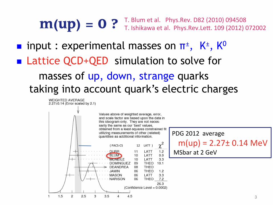
m(up) = 0 ?

n  input : experimental masses on π±, K±, K0

n  Lattice QCD+QED simulation to solve for masses of up, down, strange quarks taking into account quark’s electric charges

!"#$%&'%&""""""""""""""""""()"""""*$++"",

PDG 2012 average m(up) = 2.27± 0.14 MeV MSbar at 2 GeV

T. Blum et al. Phys.Rev. D82 (2010) 094508 T. Ishikawa et al. Phys.Rev.LeV. 109 (2012) 072002

3

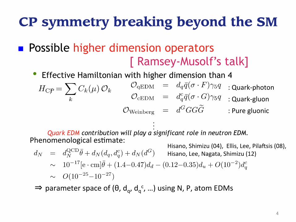
n  Possible higher dimension operators [ Ramsey-Musolf’s talk] •  Effective Hamiltonian with higher dimension than 4

Quark EDM contribution will play a significant role in neutron EDM.

CP symmetry breaking beyond the SM

: Quark-‐photon : Quark-‐gluon : Pure gluonic

Phenomenological esYmate: Hisano, Shimizu (04), Ellis, Lee, Pila\sis (08), Hisano, Lee, Nagata, Shimizu (12)

⇒ parameter space of (θ, dq, dqc, …) using N, P, atom EDMs

4

Constraint on nEDM n  The present and future experiments

are aiming to check/exclude of MSSM [ Kirch’s talk] pEDM @ BNL

nEDM @ ONL, PSI, ILL, J-PARC, TRIUMF ,FNAL, FRM2, ... charged hadrons @ COSY ⇒ a sensitivity of 10-29 e・cm !

n  Current theoretical bound is based on quark model,

non-perturbative computations of

EDM dn(θ, dq, dqc, ...)

are necessary Harris, 0709.3100

5

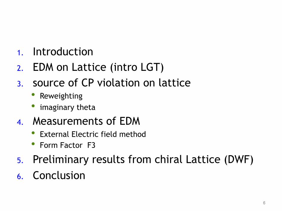
1.  Introduction 2.  EDM on Lattice (intro LGT) 3.  source of CP violation on lattice •  Reweighting •  imaginary theta

4.  Measurements of EDM •  External Electric field method •  Form Factor F3

5.  Preliminary results from chiral Lattice (DWF) 6.  Conclusion

6

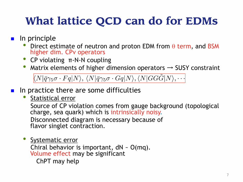
What lattice QCD can do for EDMs

n  In principle •  Direct estimate of neutron and proton EDM from θ term, and BSM

higher dim. CPv operators •  CP violating π-N-N coupling •  Matrix elements of higher dimension operators → SUSY constraint

n  In practice there are some difficulties •  Statistical error Source of CP violation comes from gauge background (topological

charge, sea quark) which is intrinsically noisy. Disconnected diagram is necessary because of

flavor singlet contraction.

•  Systematic error Chiral behavior is important, dN ~ O(mq).

Volume effect may be significant ChPT may help

7

EDM from (dynamical) lattice QCD

n  1990 Aoki-Gocksch (BNL), quenched Wilson quark, Electric field

n  2006 Berruto et al. (RBC), Nf=2 chiral quark (DWF) F3, Mπ~500 MeV

n  2006-08 Shintani et al (CP-PACS) Nf=2 Wilson-clover quark, F3 & Electric field, Mπ~500 MeV

n  2008 TI + QCDSF Nf=2 Wilson-clover quark imaginary θ, F3 & Electric field, Mπ~600 MeV on-going computations

n  2009- QCDSF n  2011- Shintani et al (RBC) Nf=2+1 chiral quarks (DWF)

Mπ ~ 300 – 180 MeV n  2012- Bhattacharya et al. BSM operators, clover-Wilson quark

8

EDM from lattice QCD

n  Three ingredients •  QCD vacuum samples •  source of CP violation

Ø  Reweighting from

CP symmetric vacuum

Ø  Dynamical simulation

•  Polarized Nucleons

n  Two methods •  Measure a spin splitting of energy

•  Form Factor

9

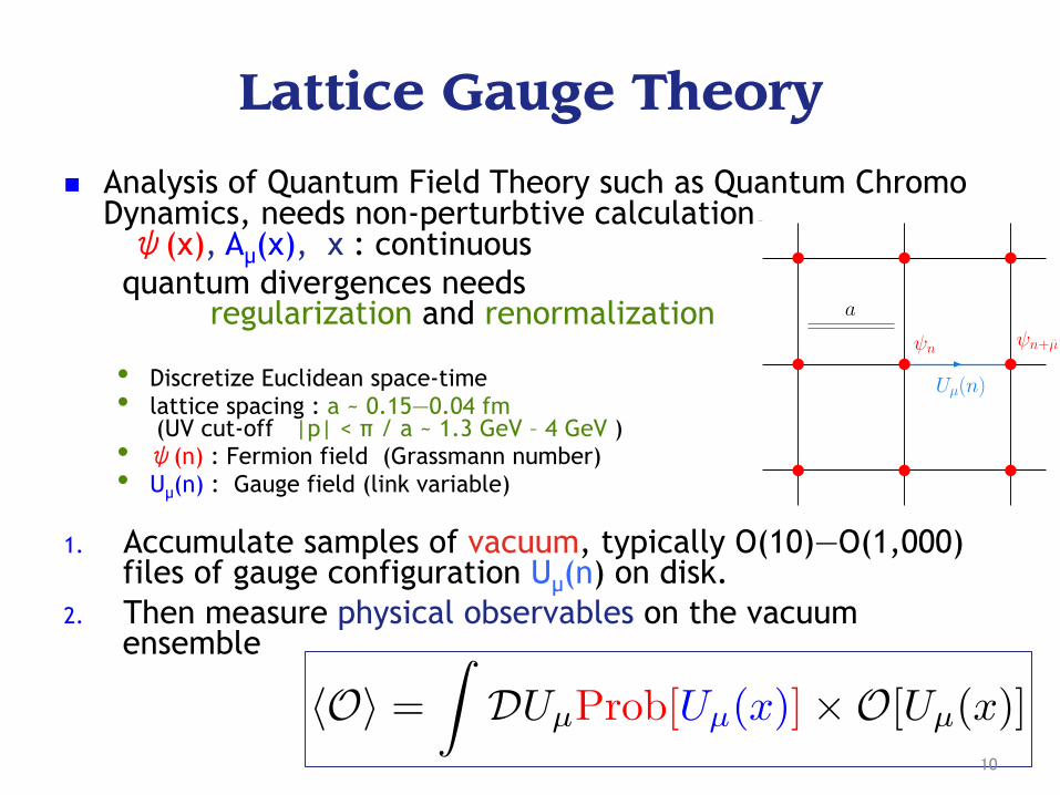
Lattice Gauge Theory

n  Analysis of Quantum Field Theory such as Quantum Chromo Dynamics, needs non-perturbtive calculation. ψ(x), Aµ(x), x : continuous

quantum divergences needs regularization and renormalization •  Discretize Euclidean space-time •  lattice spacing : a ~ 0.15—0.04 fm

(UV cut-off |p| < π / a ~ 1.3 GeV – 4 GeV ) •  ψ(n) : Fermion field (Grassmann number) •  Uµ(n) : Gauge field (link variable)

1.  Accumulate samples of vacuum, typically O(10)—O(1,000) files of gauge configuration Uµ(n) on disk.

2.  Then measure physical observables on the vacuum ensemble

!n+µ̂!n

Uµ(n)

a

10

Generation of LGT vacuum

n  Fermion (Quark) is not a floating point number (Grassmannian)→ Integrate out

n  Dirac determinant of NF quarks, det[D]N, is then stochastically evaluated by Hybrid Monte Carlo (HMC) algorithms ( lighter quark, more FLOPS)

Trajectory 0Trajectory 2

: P, Phi refresh

U

P

0 100 200 300 400 500M

PS [MeV]

0

5

10

15

20

25

[ 1

0 P

Flo

ps

ye

ars

]

CloverDWF (Ls=16)

11

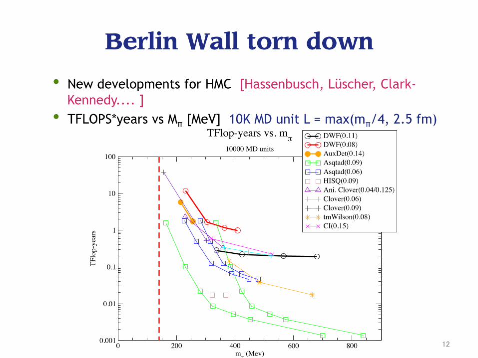
Berlin Wall torn down

•  New developments for HMC [Hassenbusch, Lüscher, Clark-Kennedy.... ] •  TFLOPS*years vs Mπ [MeV] 10K MD unit L = max(mπ/4, 2.5 fm)

0 200 400 600 800mπ

(Mev)

0.001

0.01

0.1

1

10

100

TFlo

p-ye

ars

DWF(0.11)DWF(0.08)AuxDet(0.14)Asqtad(0.09)Asqtad(0.06)HISQ(0.09)Ani. Clover(0.04/0.125)Clover(0.06)Clover(0.09)tmWilson(0.08)CI(0.15)

TFlop-years vs. mπ

10000 MD units

12

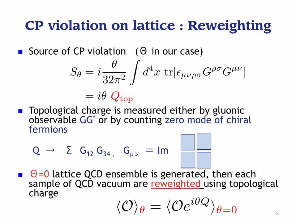
CP violation on lattice : Reweighting

n  Source of CP violation (Θ in our case)

n  Topological charge is measured either by gluonic observable GG* or by counting zero mode of chiral fermions

Q → Σ G12 G34 , Gµν　＝ Im n  Θ=0 lattice QCD ensemble is generated, then each

sample of QCD vacuum are reweighted using topological charge

13

Qtop on lattice (Θ=0)

•  Qtop history in simulation Nf=2+1 DWF, [ RBC/UKQCD] •  1/a= 1.73, 2.28 GeV •  mps =290 – 420 MeV

99

TABLE XXXVIII: Topological charge and susceptibility. The measurement frequency, “meas. freq.”, and

“block size” are given in units of Monte Carlo time.

ml meas. freq. block size !Q" !Q2" ! (GeV4)

0.005 5 50 0.49 (25) 28.6 (1.4) 0.000290 (14)

0.01 5 50 -0.22 (37) 45.2 (2.5) 0.000458 (25)

0.004 4 200 0.59 (42) 11.4 (1.1) 0.000148 (14)

0.006 4 200 -0.07 (64) 24.8 (4.3) 0.000322 (55)

0.008 4 400 0.64 (100) 27.9 (5.6) 0.000363 (72)

-20-1001020

-20-1001020

-20-1001020

-20-1001020

0 1000 2000 3000 4000 5000 6000 7000 8000 9000-20-1001020

FIG. 52: Monte Carlo time histories of the topological charge. The light sea quark mass increases from top

to bottom, (0.005 and 0.01, 243 (top two panels), and 0.004-0.008, 323). Data for the 243 ensembles up to

trajectory 5000 were reported originally in [1] and the results from the new ensembles are plotted in black.

Most of the data was generated using the RHMC II algorithm (red and black lines). The RHMC 0 (green

line) and RHMC I (blue line) algorithms were used for trajectories up to 1455 for the ml = 0.01 ensemble.

The small gap in the top panel represents missing measurements which are irrelevant since observables are

always calculated starting from trajectory 1000.

100

-20 -15 -10 -5 0 5 10 15 20Q

0

50

100

150

200

-20 -10 0 10 20Q

0

50

100

150

200

-20 -10 0 10 20Q

0

50

100

150

200

-20 -15 -10 -5 0 5 10 15 20Q

0

50

100

150

200

-20 -10 0 10 20Q

0

50

100

150

200

FIG. 53: Topological charge distributions. Top: 323, ml = 0.004! 0.008, left to right. Bottom: 243,

ml = 0.005 and 0.01.

tary pion masses in the range 290–420MeV (225–420MeV for the partially quenched pions). The

raw data obtained at each of the two values of ! was presented in Sections III and IV respectively

and the chiral behaviour of physical quantities on the 243 and 323 lattices separately was studied

in AppendixA. The main aim of this paper however, was to combine the data obtained at the

two values of the lattice spacing into global chiral–continuum fits in order to obtain results in the

continuum limit and at physical quark masses and we explain our procedure in SectionV. In that

section we define our scaling trajectory, explain how we match the parameters at the different

lattice spacings so that they correspond to the same physics and discuss how we perform the ex-

trapolations. We consider this discussion to be a significant component of this paper and believe

that this will prove to be a good approach in future efforts to obtain physical results from lattice

data. Although we apply the procedures to our data at two values of the lattice spacing, we stress

that the discussion is more general and can be used with data from simulations at an arbitrary

number of different values of ! . In the second half of SectionV we then perform the combined

continuum–chiral fits in order to obtain our physical results for the decay constants, physical bare

14

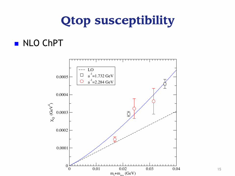
Qtop susceptibility

n  NLO ChPT 101

0 0.01 0.02 0.03 0.04ml+mres (GeV)

0

0.0001

0.0002

0.0003

0.0004

0.0005

! Q (G

eV4 )

LOa-1=1.732 GeVa-1=2.284 GeV

FIG. 54: Topological susceptibility (243 (squares), 323 (circles)). The dashed line is the prediction from LO

SU(2) chiral perturbation theory (Eq. (100)) with the chiral condensate computed from the finite volume

LEC’s given in Table XXVII. The solid line denotes the result of the single-parameter fit to the NLO

formula given in Eq. (102).

quark masses (which are renormalized in Section VI) and for the quantities r0 and r1 defined from

the heavy-quark potential. For the discussion below, it is important to recall that we use the phys-

ical pion, kaon and " masses to determine the physical quark masses and the values of the lattice

spacing and we then make predictions for other physical quantities.

In contrast to most other current lattice methods, the DWF formulation gives our simulations

good control over chiral symmetry, non-perturbative renormalization factors and flavor symmetry.

This control allows us to measure and use, as either inputs or predictions: pseudoscalar decay

constants, as well as their ratios; pseudoscalar masses; baryon masses; weak matrix elements

and static potential values, limited only by the statistics achievable for these observables. The

ability to predict many observables from the same simulations, provides evidence for the general

reliability of the underlying methods. The good properties of DWF also allow us to test scaling,

over this wide range of observables, at unphysical quark masses, since there are no flavor or chiral

symmetry breaking effects to distort a test of scaling. We find scaling violations at the percent

level, which supports including scaling corrections in only the leading order terms in our light-

quark expansions.

15

Qtop on lattice ( Imaginary θ )

n  Sθ = i Qtop : sign problem, Prob[ Uµ ] is not positive → Reweighting method

n  Alternatively, analytically continued to pure imaginary, θ → iθΙ •  Would be beneficial in terms of efficiency in Monte Carlo

important sampling

TI(07), Horsley et al. (08)

! !

"#$%!&#'(&!)#!)*%!+,!-*.&#/#-*'! 0"-#$)(1)!/("-&.123!!!!,#14%1)$()%!#1!-#.1)/!54#16.27$().#18!!9*%$%!)*%!.1)%2$(1:!./!&($2%!

! 01!7/7(&!;,<!/."7&().#1!#1&'!!!!!!!!(4).#1!-($)=!!!!!!!!!!./!7/%:!6#$!2%1%$().12!>(477"%!%1/%"?&%=!(1:!&()%$!)*%!@#?/%$>(?&%A!-($)=!!!!!!!!!=!./!"%(/7$%:B

! !."-#$)(1)!/("-&.12!1#)!#1&'!6#$!(4).#1!?7)!(&/#!6#$!)*%!"%(/7$%"%1)B!C7/).6.(?&%!6#$!:.66.47&)!-$#?&%"/!D

! ! ""!!!

!"# !

!##$ $"!!!"!!!"

"!!!"

16

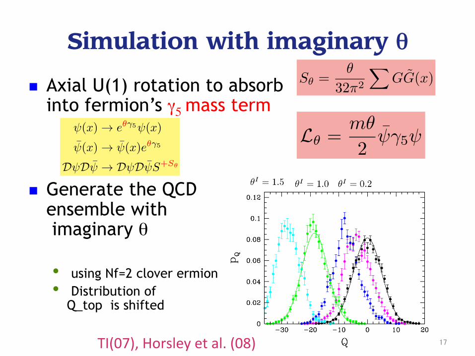
Simulation with imaginary θ

n  Axial U(1) rotation to absorb into fermion’s γ5 mass term

n  Generate the QCD ensemble with imaginary θ

•  using Nf=2 clover ermion •  Distribution of

Q_top is shifted

TI(07), Horsley et al. (08) 17

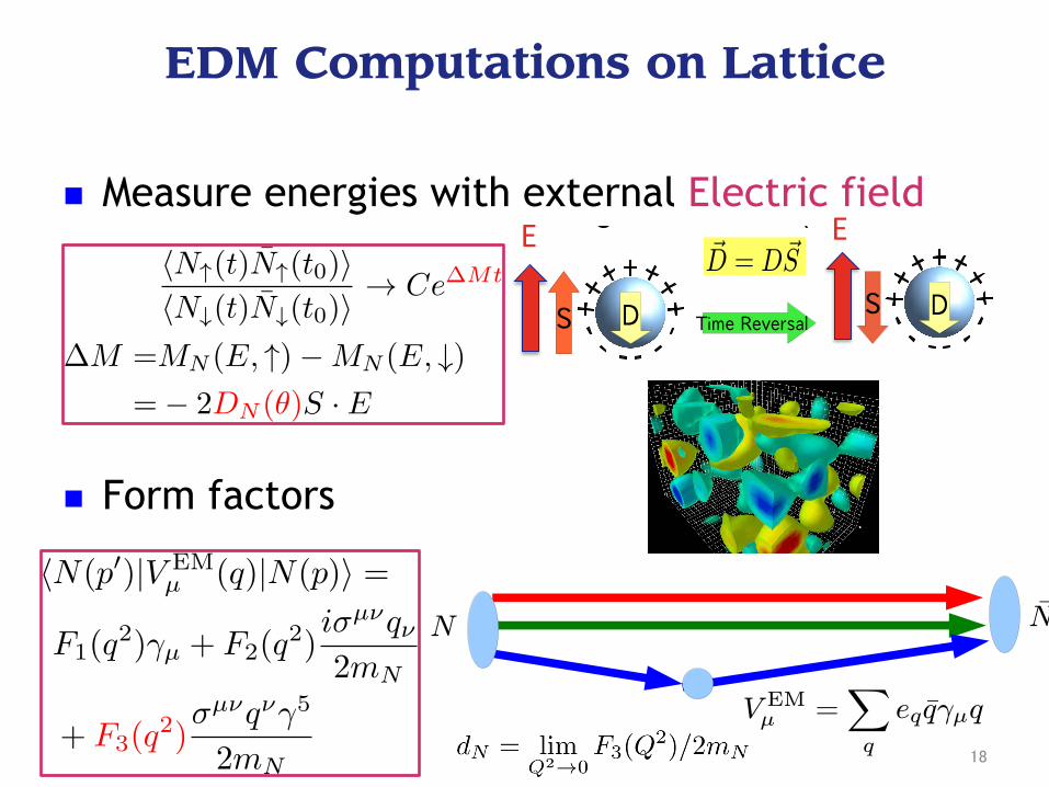
EDM Computations on Lattice

n  Measure energies with external Electric field

n  Form factors

!"#$#%&'()$"#%*+,-*#%*./$$01(

*!("2/%(%$*+3(1$"01*,04#3(*-#2(%$*5+,-6*07*/*708%/$)"(*#9*:!*5#"*;02(*"(<("7/36**7=22($"=*<0#3/$0#%>

?*7#)"1(*#9**:!*<0#3/$0#%*@

Strong CP: vacuum angle ! , is implemented on lattice with analytically continued to pure imaginary (Monte Carlo simulation)

+,-*07*2(/7)"(A*$B"#)8B*$B(*(3(1$"01*9#"2*9/1$#"*C!"D#$

**

!" #$%&'(&)&*+,-

!" % "!#

!" !!"

$ ! "%$

$ % &&'' &&(' (&)' (&#' (&(

!(!")

!$#* "#$ "+$#( !")$"

%% ,!"+

"$-$ * ,""+"$+&.$&#/'

* %$,#"+"$+&.$&-$#/'

* $ $ $ ' + % )! " )

"( % +,-)!"%

0

#/'

,#"+"$

(.(

* &'$ %#

)

0).+-$+

!"#$#%&'()$"#%*+,-*#%*./$$01(

*!("2/%(%$*+3(1$"01*,04#3(*-#2(%$*5+,-6*07*/*708%/$)"(*#9*:!*5#"*;02(*"(<("7/36**7=22($"=*<0#3/$0#%>

?*7#)"1(*#9**:!*<0#3/$0#%*@

Strong CP: vacuum angle ! , is implemented on lattice with analytically continued to pure imaginary (Monte Carlo simulation)

+,-*07*2(/7)"(A*$B"#)8B*$B(*(3(1$"01*9#"2*9/1$#"*C!"D#$

**

!" #$%&'(&)&*+,-

!" % "!#

!" !!"

$ ! "%$

$ % &&'' &&(' (&)' (&#' (&(

!(!")

!$#* "#$ "+$#( !")$"

%% ,!"+

"$-$ * ,""+"$+&.$&#/'

* %$,#"+"$+&.$&-$#/'

* $ $ $ ' + % )! " )

"( % +,-)!"%

0

#/'

,#"+"$

(.(

* &'$ %#

)

0).+-$+

E E

18

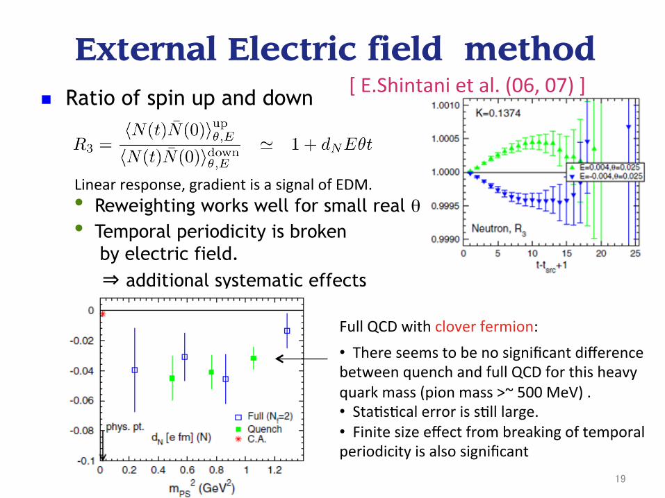
n  Ratio of spin up and down

•  Reweighting works well for small real θ •  Temporal periodicity is broken

by electric field. ⇒ additional systematic effects

External Electric field method

•  There seems to be no significant difference between quench and full QCD for this heavy quark mass (pion mass >~ 500 MeV) . •  StaYsYcal error is sYll large. •  Finite size effect from breaking of temporal periodicity is also significant

Linear response, gradient is a signal of EDM.

Full QCD with clover fermion:

[ E.Shintani et al. (06, 07) ]

19

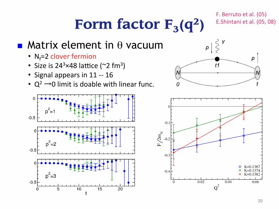
n  Matrix element in θ vacuum

F. Berruto et al. (05) E.Shintani et al. (05, 08) Form factor F3(q

2)

•  Nf=2 clover fermion •  Size is 243×48 lakce (~2 fm3) •  Signal appears in 11 -‐-‐ 16 •  Q2 →0 limit is doable with linear func.

20

n  Full QCD with Wilson fermion

Imaginary θ Izubuchi(07), Horsley et al. (08)

Nf=2, 163×32 lakce, mπ = 700 MeV Fermionic inserYon of imaginary theta:

21

The Electric Dipole Moment of the Neutron

Chiral symmetry: rotation of valencequark fields (sources) renders valence θVunobservable.

Z(η̄, η) =�

DAµ det (/D +m+ iθγ5m)

exp η̄(/D +m+ iθV γ5m)−1η

η → e−iγ5θV /2η

Wilson fermions break chiral symmetry.dN for θV �= 0 mainly lattice artifact[Aoki, et al. (1990)].

Signal disappears for θV = 0 (θsea = 0.4)

[Izubuchi, et al., (2008)]

13

Effects from valence theta

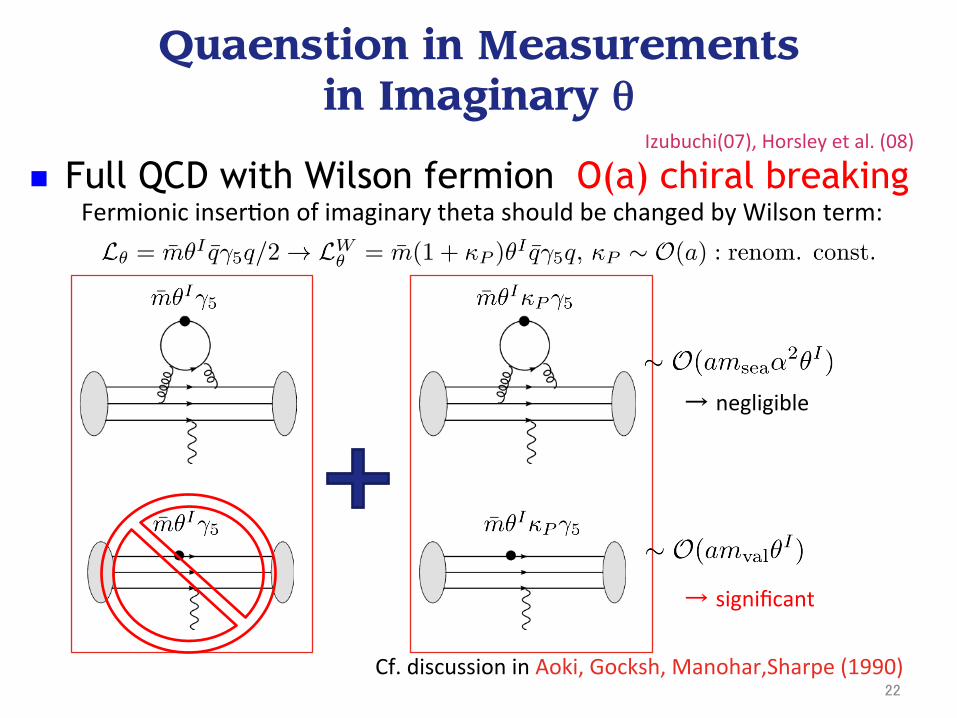
n  Full QCD with Wilson fermion O(a) chiral breaking

Quaenstion in Measurements in Imaginary θ

Fermionic inserYon of imaginary theta should be changed by Wilson term:

Cf. discussion in Aoki, Gocksh, Manohar,Sharpe (1990) 22

→ negligible

→ significant

Izubuchi(07), Horsley et al. (08)

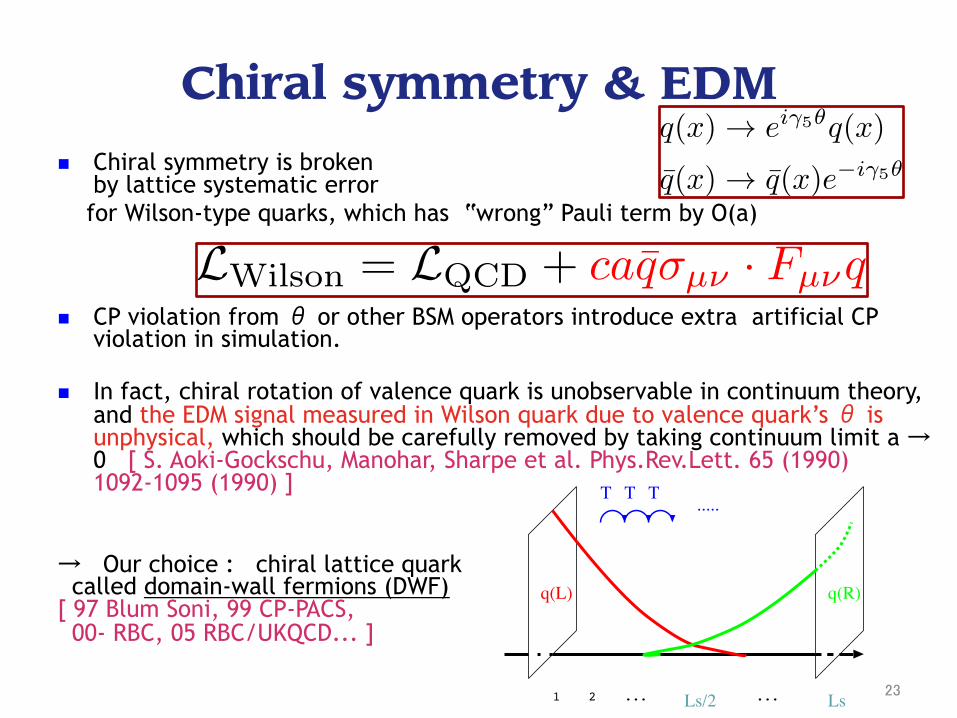
Chiral symmetry & EDM

n  Chiral symmetry is broken by lattice systematic error

for Wilson-type quarks, which has “wrong” Pauli term by O(a) n  CP violation from θ or other BSM operators introduce extra artificial CP

violation in simulation.

n  In fact, chiral rotation of valence quark is unobservable in continuum theory, and the EDM signal measured in Wilson quark due to valence quark’s θ is unphysical, which should be carefully removed by taking continuum limit a → 0 [ S. Aoki-Gockschu, Manohar, Sharpe et al. Phys.Rev.Lett. 65 (1990) 1092-1095 (1990) ]

→ Our choice : chiral lattice quark called domain-wall fermions (DWF) [ 97 Blum Soni, 99 CP-PACS, 00- RBC, 05 RBC/UKQCD... ]

1 2 Ls/2 Ls... ...

q(L) q(R)

T T T .....

23

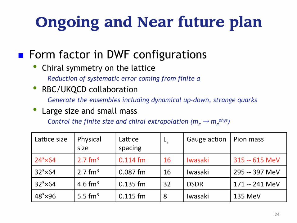
n  Form factor in DWF configurations •  Chiral symmetry on the lattice

Reduction of systematic error coming from finite a

•  RBC/UKQCD collaboration Generate the ensembles including dynamical up-down, strange quarks

•  Large size and small mass Control the finite size and chiral extrapolation (mπ → mπ

phys)

Ongoing and Near future plan

Lakce size Physical size

Lakce spacing

Ls Gauge acYon Pion mass

243×64 2.7 fm3 0.114 fm 16 Iwasaki 315 -‐-‐ 615 MeV

323×64 2.7 fm3 0.087 fm 16 Iwasaki 295 -‐-‐ 397 MeV

323×64 4.6 fm3 0.135 fm 32 DSDR 171 -‐-‐ 241 MeV

483×96 5.5 fm3 0.115 fm 8 Iwasaki 135 MeV

24

Difficulties in EDM calculations

n  Very sensitive to chiral symmetry n  Intrinsically noisy, theta is only affecting to

Nucleon observable indirectly, in contrast to the case of (Chromo) quark EDMs.

n  To avoid the excited state contamination, one needs to separate Nucleons and the EM current.

But signal to noise degrates exponentially [Lepage]

25

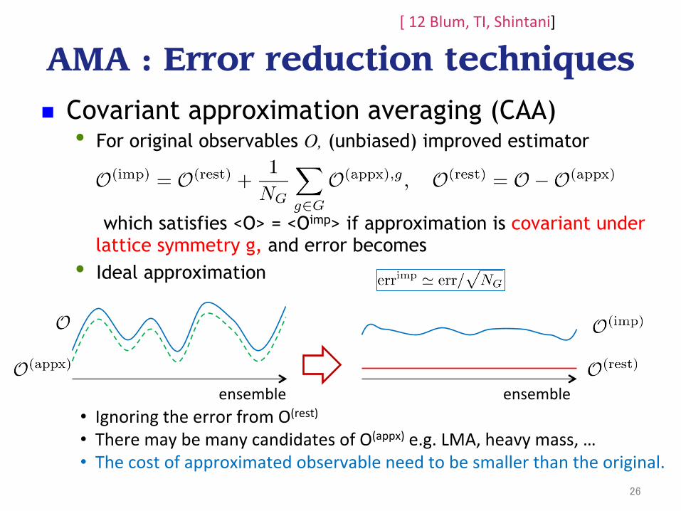
AMA : Error reduction techniques

n  Covariant approximation averaging (CAA) •  For original observables O, (unbiased) improved estimator

which satisfies <O> = <Oimp> if approximation is covariant under

lattice symmetry g, and error becomes •  Ideal approximation

ensemble ensemble •  Ignoring the error from O(rest) •  There may be many candidates of O(appx) e.g. LMA, heavy mass, … •  The cost of approximated observable need to be smaller than the original.

[ 12 Blum, TI, Shintani]

26

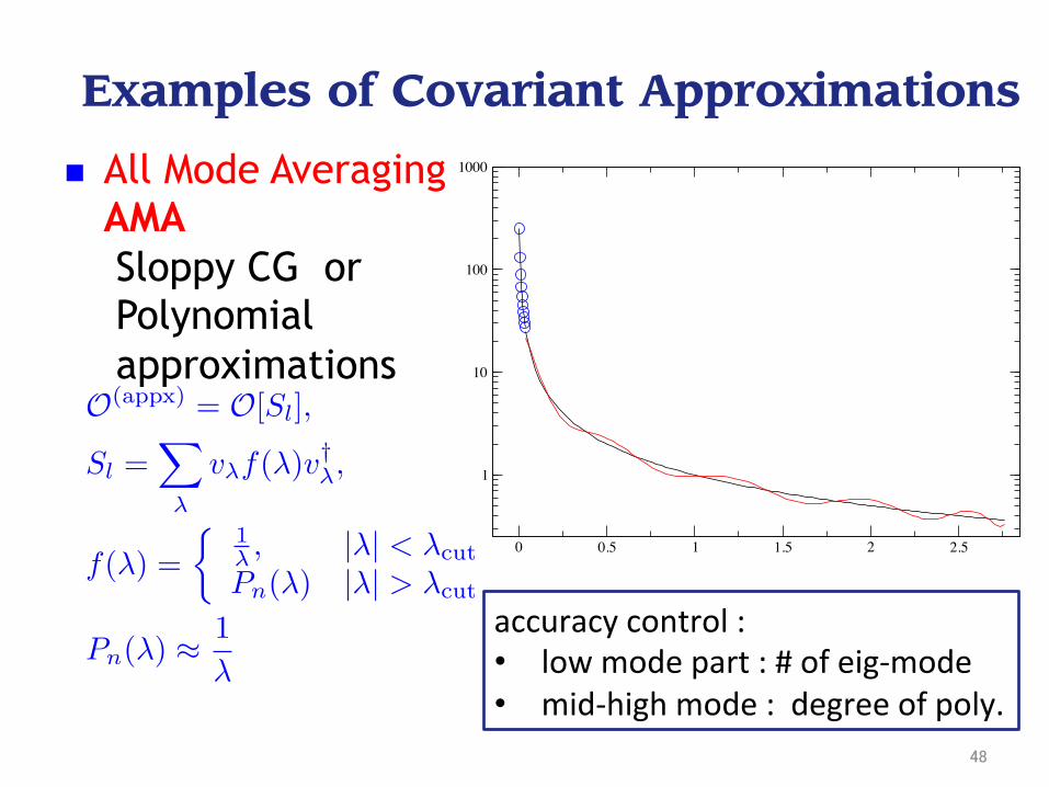
Examples of Covariant Approximations

n  All Mode Averaging AMA Sloppy CG or Polynomial approximations

0 0.5 1 1.5 2 2.5

1

10

100

1000

Figure 3: Polynomial approximation of 1/λ, Npoly = 10, the mini-max approximation forthe relative error, for λ ∈ [0.052, 1.672].

8

accuracy control : •  low mode part : # of eig-‐mode •  mid-‐high mode : degree of poly.

27

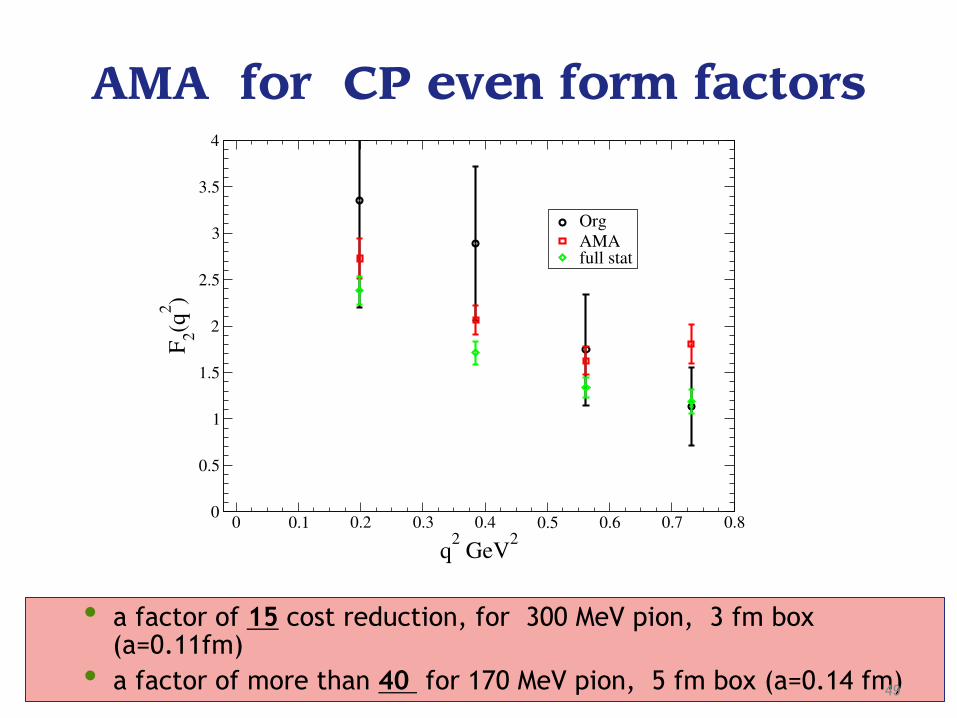
AMA for CP even form factors

•  a factor of 15 cost reduction, for 300 MeV pion, 3 fm box (a=0.11fm) •  a factor of more than 40 for 170 MeV pion, 5 fm box (a=0.14 fm)

0 0.1 0.2 0.3 0.4 0.5 0.6 0.7 0.8

q2 GeV

2

0

0.5

1

1.5

2

2.5

3

3.5

4

F2(q

2)

OrgAMAfull stat

28

Hadronic vacuum polarization( AsqTad )

0 2 4 6 8 10Q2 (GeV2)

0.06

0.08

0.1

0.12

0.14

0.16

0.18

0.2

-Π(Q

2 )

0 0.2 0.40.14

0.16

0.18

0.2

29

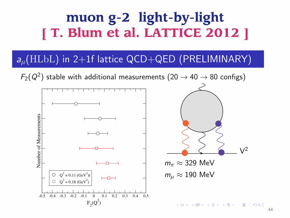
muon g-2 light-by-light [ T. Blum et al. LATTICE 2012 ]

IntroductionThe hadronic vacuum polarization (HVP) contribution (O(α2))

The hadronic light-by-light (HLbL) contribution (O(α3))aµ Implications for new physics

Summary/Outlook

aµ(HLbL) in 2+1f lattice QCD+QED (PRELIMINARY)

F2(Q2) stable with additional measurements (20 → 40 → 80 configs)

-0.5 -0.4 -0.3 -0.2 -0.1 0 0.1 0.2 0.3 0.4 0.5

F2(Q2)

Num

ber o

f Mea

sure

men

ts

Q2 = 0.11 (GeV2)tQ2 = 0.18 (GeV2)

243 lattice size

Q2 = 0.11 and 0.18 GeV2

mπ ≈ 329 MeV

mµ ≈ 190 MeV

Tom Blum (UConn and RIKEN BNL Research Center) The muon anomalous magnetic moment



Summary/Outlook



-0.5 -0.4 -0.3 -0.2 -0.1 0 0.1 0.2 0.3 0.4 0.5

F2(Q2)

Num

ber o

f Mea

sure

men

ts

Q2 = 0.11 (GeV2)tQ2 = 0.18 (GeV2)

243 lattice size

Q2 = 0.11 and 0.18 GeV2

mπ ≈ 329 MeV

mµ ≈ 190 MeV

Tom Blum (UConn and RIKEN BNL Research Center) The muon anomalous magnetic moment30

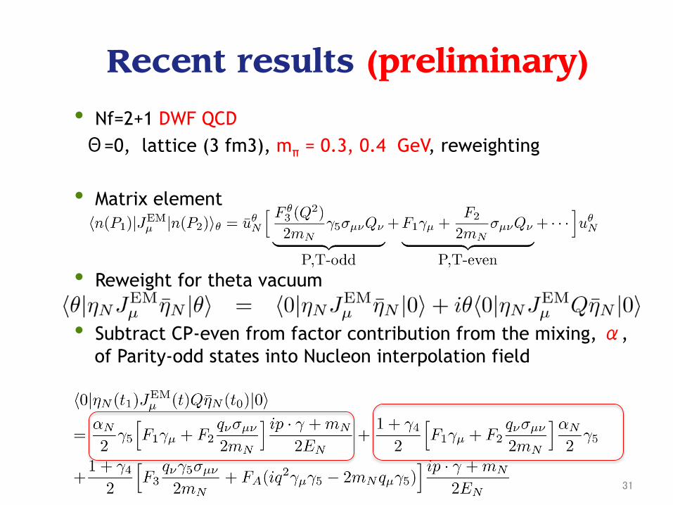
•  Nf=2+1 DWF QCD Θ=0, lattice (3 fm3), mπ = 0.3, 0.4 GeV, reweighting •  Matrix element •  Reweight for theta vacuum •  Subtract CP-even from factor contribution from the mixing, α,

of Parity-odd states into Nucleon interpolation field

31

Recent results (preliminary)

mixing of parity-odd states α n  Nucleon interpolation field

in CP-even work.

n  When CP is violated, N and P-odd states (N*, N+π,...) mix [ 99 Pospelov Ritz ]

n  Nucleon 2pt function with θ reweighting

•  α which is CP-odd phase is necessary to extract EDM form factor. •  It is good check of applicability of LMA/AMA to CP-odd sector. •  Effective mass plot shows the consistency of the above formula

32

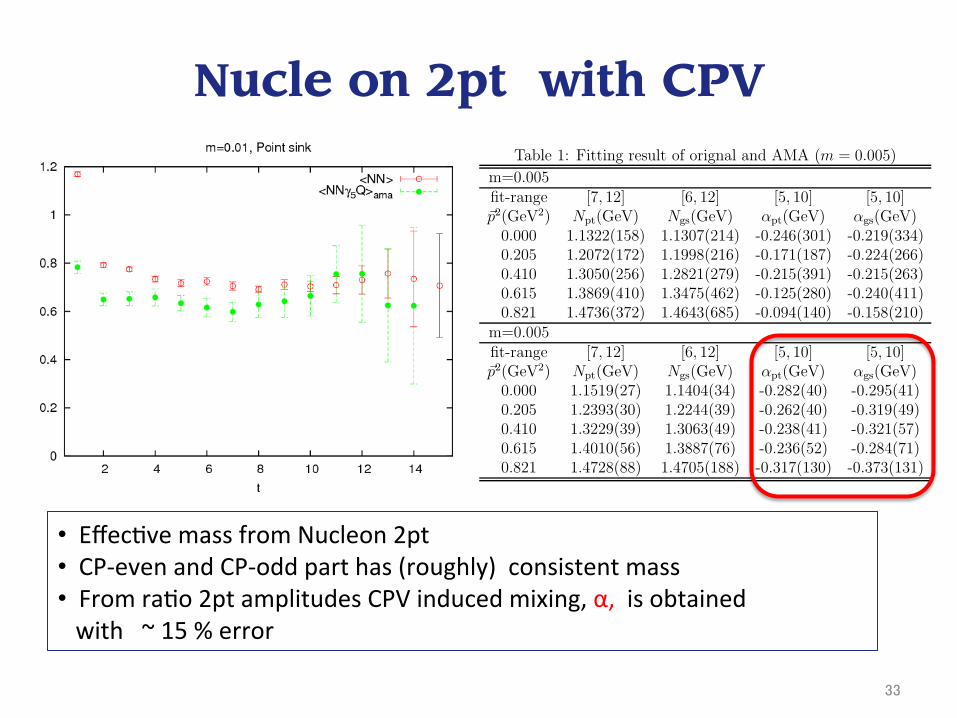
Nucle on 2pt with CPV

•  EffecYve mass from Nucleon 2pt •  CP-‐even and CP-‐odd part has (roughly) consistent mass •  From raYo 2pt amplitudes CPV induced mixing, α, is obtained with ~ 15 % error

33

Table 1: Fitting result of orignal and AMA (m = 0.005)

m=0.005fit-range [7, 12] [6, 12] [5, 10] [5, 10]!p2(GeV2) Npt(GeV) Ngs(GeV) "pt(GeV) "gs(GeV)

0.000 1.1322(158) 1.1307(214) -0.246(301) -0.219(334)0.205 1.2072(172) 1.1998(216) -0.171(187) -0.224(266)0.410 1.3050(256) 1.2821(279) -0.215(391) -0.215(263)0.615 1.3869(410) 1.3475(462) -0.125(280) -0.240(411)0.821 1.4736(372) 1.4643(685) -0.094(140) -0.158(210)

m=0.005fit-range [7, 12] [6, 12] [5, 10] [5, 10]!p2(GeV2) Npt(GeV) Ngs(GeV) "pt(GeV) "gs(GeV)

0.000 1.1519(27) 1.1404(34) -0.282(40) -0.295(41)0.205 1.2393(30) 1.2244(39) -0.262(40) -0.319(49)0.410 1.3229(39) 1.3063(49) -0.238(41) -0.321(57)0.615 1.4010(56) 1.3887(76) -0.236(52) -0.284(71)0.821 1.4728(88) 1.4705(188) -0.317(130) -0.373(131)

Table 2: EM form factor result of orignal and AMA (m = 0.005)

m=0.005P N

fit-range [4, 8] [4, 8] [4, 8] [4, 8]q2(GeV2) Ge Gm Ge Gm

-0.199 0.486(192) 1.295(524) 0.028(18) -0.798(334)-0.380 0.326(206) 0.987(621) 0.030(24) -0.591(378)-0.550 0.245(115) 0.764(355) 0.049(32) -0.419(199)-0.704 0.122(98) 0.433(387) 0.037(40) -0.269(237)

m=0.005P N

fit-range [4, 8] [4, 8] [4, 8] [4, 8]q2(GeV2) Ge Gm Ge Gm

-0.197 0.722(11) 1.916(43) 0.007( 3) -1.212(30)-0.381 0.559( 9) 1.483(34) 0.014( 4) -0.956(23)-0.553 0.435(11) 1.179(39) 0.025( 5) -0.784(29)-0.718 0.374(14) 1.027(51) 0.021( 7) -0.640(33)

18

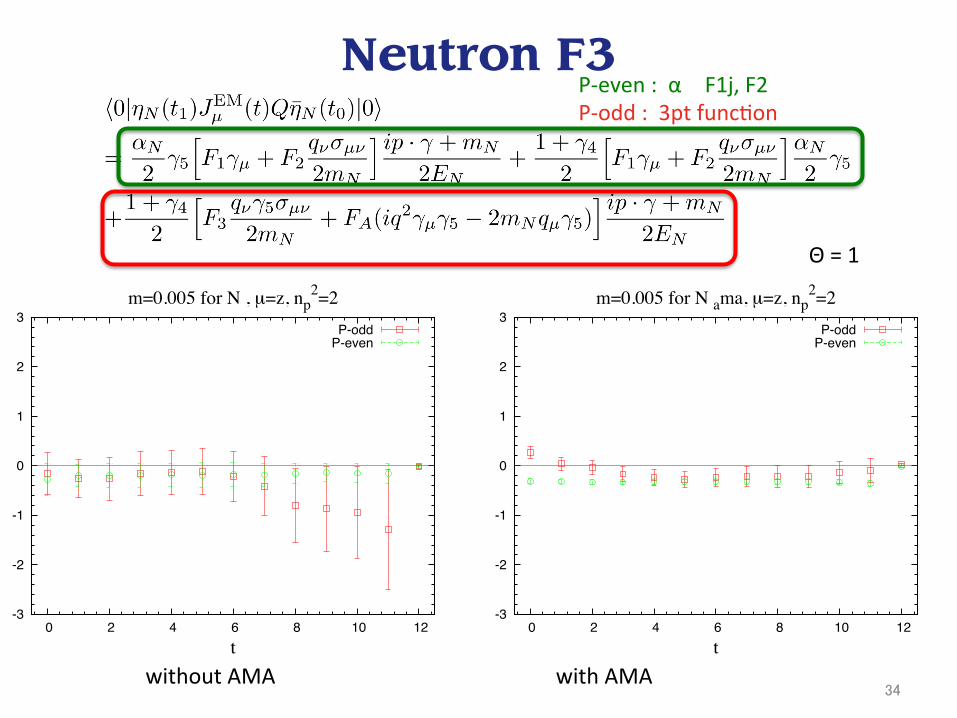
Neutron F3 P-‐even : α　 F1j, F2 P-‐odd : 3pt funcYon

without AMA with AMA

-3

-2

-1

0

1

2

3

0 2 4 6 8 10 12t

m=0.005 for N , µ=z, np2=1

P-oddP-even

-3

-2

-1

0

1

2

3

0 2 4 6 8 10 12t

m=0.005 for N ama, µ=z, np2=1

P-oddP-even

-3

-2

-1

0

1

2

3

0 2 4 6 8 10 12t

m=0.005 for N , µ=z, np2=2

P-oddP-even

-3

-2

-1

0

1

2

3

0 2 4 6 8 10 12t


P-oddP-even

-3

-2

-1

0

1

2

3

0 2 4 6 8 10 12t

m=0.005 for N , µ=z, np2=3

P-oddP-even

-3

-2

-1

0

1

2

3

0 2 4 6 8 10 12t


P-oddP-even

Figure 4: Neutron EDM form factor.

12

Θ = 1

34

Proton F3

•  Noisier than Neutron (stronger α, but weaker CPV 3pt)

-3

-2

-1

0

1

2

3

0 2 4 6 8 10 12t

m=0.005 for P , µ=z, np2=1

P-oddP-even

-3

-2

-1

0

1

2

3

0 2 4 6 8 10 12t

m=0.005 for P ama, µ=z, np2=1

P-oddP-even

-3

-2

-1

0

1

2

3

0 2 4 6 8 10 12t

m=0.005 for P , µ=z, np2=2

P-oddP-even

-3

-2

-1

0

1

2

3

0 2 4 6 8 10 12t


P-oddP-even

-3

-2

-1

0

1

2

3

0 2 4 6 8 10 12t

m=0.005 for P , µ=z, np2=3

P-oddP-even

-3

-2

-1

0

1

2

3

0 2 4 6 8 10 12t


P-oddP-even

Figure 6: Proton EDM form factor.

14

35

Statistical signal check •  Mpi = 330 MeV, a=0.11 fm, V=(3fm)3

•  191 config * 32 measurements vs 380 config * 32 measurements •  green: from Vt, blue: from Vz

-0.3

-0.2

-0.1

0

0.1

0.2

0.3

0 2 4 6 8 10 12

F 3/2

mN

(e fm

)

t

m=0.005 for N , np2=1

tz

-0.3

-0.2

-0.1

0

0.1

0.2

0.3

0 2 4 6 8 10 12F 3

/2m

N (e

fm)

t

m=0.005 for N ama, np2=1

tz

-0.3

-0.2

-0.1

0

0.1

0.2

0.3

0 2 4 6 8 10 12

F 3/2

mN

(e fm

)

t

m=0.005 for N , np2=2

tz

-0.3

-0.2

-0.1

0

0.1

0.2

0.3

0 2 4 6 8 10 12

F 3/2

mN

(e fm

)

t


tz

-0.3

-0.2

-0.1

0

0.1

0.2

0.3

0 2 4 6 8 10 12

F 3/2

mN

(e fm

)

t

m=0.005 for N , np2=3

tz

-0.3

-0.2

-0.1

0

0.1

0.2

0.3

0 2 4 6 8 10 12

F 3/2

mN

(e fm

)

t


tz


16

-0.3

-0.2

-0.1

0

0.1

0.2

0.3

0 2 4 6 8 10 12

F 3/2

mN

(e fm

)

t

m=0.005 for N , np2=1

tz

-0.3

-0.2

-0.1

0

0.1

0.2

0.3

0 2 4 6 8 10 12F 3

/2m

N (e

fm)

t


tz

-0.3

-0.2

-0.1

0

0.1

0.2

0.3

0 2 4 6 8 10 12

F 3/2

mN

(e fm

)

t

m=0.005 for N , np2=2

tz

-0.3

-0.2

-0.1

0

0.1

0.2

0.3

0 2 4 6 8 10 12

F 3/2

mN

(e fm

)

t


tz

-0.3

-0.2

-0.1

0

0.1

0.2

0.3

0 2 4 6 8 10 12

F 3/2

mN

(e fm

)

t

m=0.005 for N , np2=3

tz

-0.3

-0.2

-0.1

0

0.1

0.2

0.3

0 2 4 6 8 10 12

F 3/2

mN

(e fm

)

t


tz


16

36

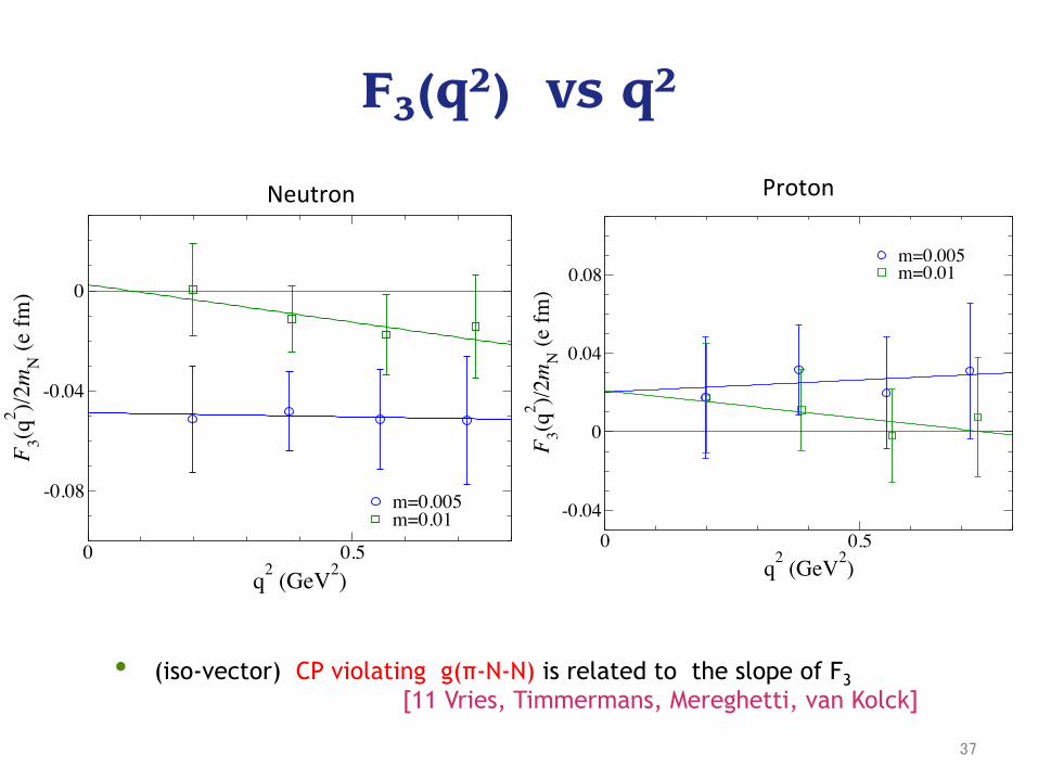
F3(q2) vs q2

•  (iso-vector) CP violating g(π-N-N) is related to the slope of F3 [11 Vries, Timmermans, Mereghetti, van Kolck]

0 0.5q2 (GeV2)

-0.08

-0.04

0

F 3(q2 )/2

mN

(e fm

)

m=0.005m=0.01

0 0.5q2 (GeV2)

-0.04

0

0.04

0.08

F 3(q2 )/2

mN

(e fm

)

m=0.005m=0.01

Figure 28: F3(q2) for neutron (top), proton (bottom).

41

0 0.5q2 (GeV2)

-0.08

-0.04

0

F 3(q2 )/2

mN

(e fm

)

m=0.005m=0.01

0 0.5q2 (GeV2)

-0.04

0

0.04

0.08

F 3(q2 )/2

mN

(e fm

)

m=0.005m=0.01

Figure 28: F3(q2) for neutron (top), proton (bottom).

41

Neutron Proton

37

0 0.2 0.4 0.6 0.8 1m!

2(GeV2)

-0.08

-0.06

-0.04

-0.02

0

0.02

0.04

0.06

0.08

0.1

d N(e

fm)

CP-PACS, Nf=2 clover, "E(#)CP-PACS, Nf=2 clover, F3(#)RBC, Nf=2 DW, F3(#)QCDSF, Nf=2 clover, F3(i#)Current algebraNf=3 DWF, F3(#)

0 0.2 0.4 0.6 0.8 1m!

2(GeV2)

-0.04

-0.02

0

0.02

0.04

0.06

0.08

0.1

d P(e fm

)

Nf=3 DWF, F3(#)CP-PACS, Nf=2 clover, F3(#)

Figure 29: dN for neutron and proton

42

n  Full QCD

Comparison of results

•  Lakce results are consistent within 1σ. (not include systemaYc error) •  larger than the results of QCD Sum Rules or ChPT.

• no obvious quark mass dependence yet staYsYcs ? • Nf = 2+1 DWF configs. (RBC/UKQCD) are available for near physical pion mass (170 MeV) is examined now.

Θ = 1 PRELIMINARY

38

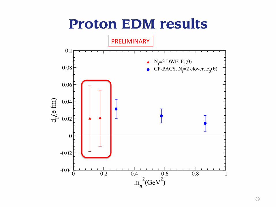
Proton EDM results 0 0.2 0.4 0.6 0.8 1m!

2(GeV2)

-0.08

-0.06

-0.04

-0.02

0

0.02

0.04

0.06

0.08

0.1

d N(e

fm)

CP-PACS, Nf=2 clover, "E(#)CP-PACS, Nf=2 clover, F3(#)RBC, Nf=2 DW, F3(#)QCDSF, Nf=2 clover, F3(i#)Current algebraNf=3 DWF, F3(#)

0 0.2 0.4 0.6 0.8 1m!

2(GeV2)

-0.04

-0.02

0

0.02

0.04

0.06

0.08

0.1d P(e

fm)

Nf=3 DWF, F3(#)CP-PACS, Nf=2 clover, F3(#)

Figure 29: dN for neutron and proton

42

PRELIMINARY

39

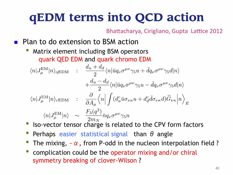
n  Plan to do extension to BSM action •  Matrix element including BSM operators

quark QED EDM and quark chromo EDM

•  Iso-vector tensor charge is related to the CPV form factors •  Perhaps easier statistical signal than θ angle •  The mixing, ~α, from P-odd in the nucleon interpolation field ? •  complication could be the operator mixing and/or chiral

symmetry breaking of clover-Wilson ?

qEDM terms into QCD action BhaVacharya, Cirigliano, Gupta Lakce 2012

40

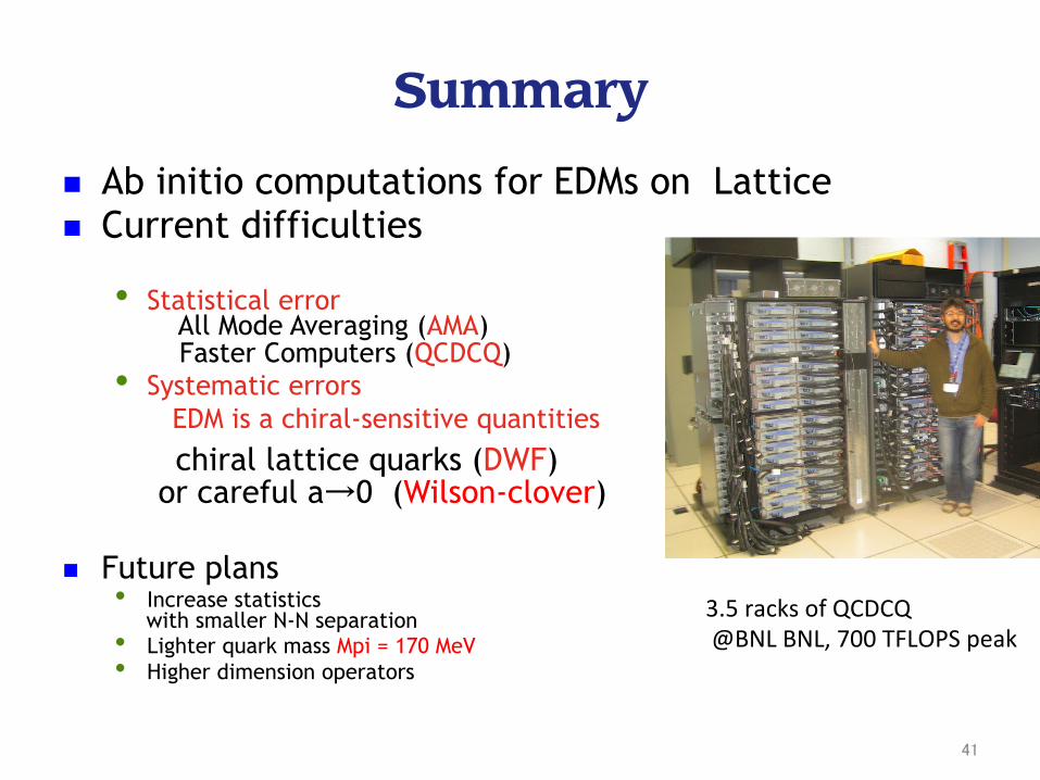
Summary

n  Ab initio computations for EDMs on Lattice n  Current difficulties

•  Statistical error

All Mode Averaging (AMA) Faster Computers (QCDCQ)

•  Systematic errors EDM is a chiral-sensitive quantities

chiral lattice quarks (DWF) or careful a→0 (Wilson-clover) n  Future plans

•  Increase statistics with smaller N-N separation

•  Lighter quark mass Mpi = 170 MeV •  Higher dimension operators

3.5 racks of QCDCQ @BNL BNL, 700 TFLOPS peak

41

BACK UP SLIDES

42

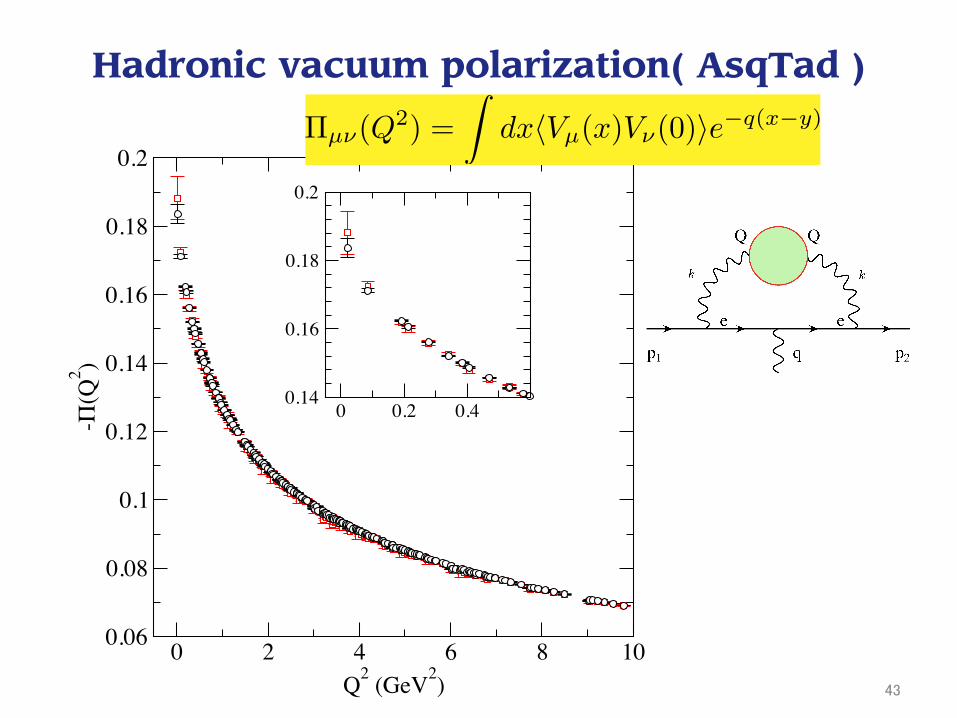
Hadronic vacuum polarization( AsqTad )

0 2 4 6 8 10Q2 (GeV2)

0.06

0.08

0.1

0.12

0.14

0.16

0.18

0.2

-Π(Q

2 )

0 0.2 0.40.14

0.16

0.18

0.2

43

muon g-2 light-by-light [ T. Blum et al. LATTICE 2012 ]



Summary/Outlook



-0.5 -0.4 -0.3 -0.2 -0.1 0 0.1 0.2 0.3 0.4 0.5

F2(Q2)

Num

ber o

f Mea

sure

men

ts

Q2 = 0.11 (GeV2)tQ2 = 0.18 (GeV2)

243 lattice size

Q2 = 0.11 and 0.18 GeV2

mπ ≈ 329 MeV

mµ ≈ 190 MeV

Tom Blum (UConn and RIKEN BNL Research Center) The muon anomalous magnetic moment



Summary/Outlook



-0.5 -0.4 -0.3 -0.2 -0.1 0 0.1 0.2 0.3 0.4 0.5

F2(Q2)

Num

ber o

f Mea

sure

men

ts

Q2 = 0.11 (GeV2)tQ2 = 0.18 (GeV2)

243 lattice size

Q2 = 0.11 and 0.18 GeV2

mπ ≈ 329 MeV

mµ ≈ 190 MeV

Tom Blum (UConn and RIKEN BNL Research Center) The muon anomalous magnetic moment44

Cost comparison for test cases n  x 16 for DWF Nucleon mass (MPS=330MeV, 3fm) n  x 2- 20 for AsqTad HVP (MPS=470 MeV, 5 fm) n  should be better for lighter mass & larger volume ?

5

TABLE IV. Computational cost. The unit of cost is one quarkpropagator without deflated CG, per configuration. NG = 32for nucleon masses and 708 for HVP. The last column givesthe cost to achieve the same error for each method, normalizedto [2] (nucleon mass mN ) and [1] (HVP) and scaled by the er-rors in Tab. III. HVP scaled costs are maximum and minimumin the range Q2 = 0 − 1 GeV2. For m = 0.005, in [2], non-relativistic spinors were used which means the scaled costs inthis case were increased by two. The cost of O(appx)

G for AMAis split to show the sloppy CG and low-mode costs separately.

Nconf Nmeas LM O O(appx)G Tot. scaled cost

mN m = 0.005, 400 LM gauss pt

AMA 110 1 213 18 91+23 350 0.063 0.065

LMA 110 1 213 18 23 254 0.279 0.265

Ref. [2] 932 4 - 3728 - 3728a 1 1

m = 0.01, 180 LM

AMA 158 1 297 74 300+22 693 0.203 0.214

LMA 158 1 297 74 22 393 0.699 0.937

Ref. [2] 356 4 - 1424 - 1424 1 1

HVP m = 0.0036, 1400 LM max min

AMA 20 1 96 11 504+420 1031 0.387 0.050

LMA 20 1 96 11 420 527 10.3 3.56

Ref. [1] 292 2 - 584 - 584 1 1

a In [2] a doubled source was used to reduce this cost by two.

covariant under lattice symmetries. This is a general-ization of low-mode averaging which reduces the statisti-cal error for observables that are not dominated by low-modes. We have shown through several numerical ex-amples that all-mode averaging is a powerful exampleof CAA, performing better than LMA and works welleven in cases where LMA fails. In the examples givenhere, AMA reduced the cost by factors up to ∼ 20, overconventional computations, and these factors will onlyincrease for larger lattice sizes and smaller quark masses.The method has great potential for investigations of dif-ficult but important physics problems where statisticalfluctuations still dominate the total uncertainty, like thenucleon electric dipole moment or hadronic contributionsto the muon anomalous magnetic moment. Since CAAworks without introducing any statistical bias (so longas condition appx-3 holds), there are many possibilitiesthat also satisfy appx-1 and appx-2: One can constructO(appx) using different lattice fermions and parameters(mass, Ls (for DWF), boundary conditions and so on).

�O(appx)G � can be measured on a larger number of gauge

configurations, which is potentially advantageous for ob-servables dominated by gauge noise such as disconnecteddiagrams. One may also consider other types of approx-imations such as the hopping parameter expansion usedin [21], or approximations at the level of hadronic Green’sfunctions.

Numerical calculations were performed using the RICC

at RIKEN and the Ds cluster at FNAL. We thank SinyaAoki, Rudy Arthur, Gunnar Bali, Peter Boyle, Nor-man Christ, Thomas DeGrand, Leonardo Giusti, ShojiHashimoto, Tomomi Ishikawa, Chulwoo Jung, TakashiKaneko, Christoph Lehner, Meifeng Lin, Stefan Schaefer,Ruth Van de Water, Oliver Witzel, Takeshi Yamazaki,Jianglei Yu and other members of JLQCD,RBC,UKQCDcollaborations for valuable discussions and comments.CPS QCD library [27] and other softwares (QMP,QIO)are used, which are supported by USQCD and US-DOE SciDAC program. This work was supported bythe Japanese Ministry of Education Grant-in-Aid, Nos.22540301 (TI), 23105714 (ES), 23105715 (TI) and U.S.DOE grants DE-AC02-98CH10886 (TI) and DE-FG02-92ER40716 (TB). We also thank BNL, the RIKEN BNLResearch Center, and USQCD for providing resourcesnecessary for completion of this work.

[1] C. Aubin, T. Blum, M. Golterman, and S. Peris, (2012),arXiv:1205.3695 [hep-lat].

[2] T. Yamazaki, Y. Aoki, T. Blum, H.-W. Lin, S. Ohta,et al., Phys.Rev. D79, 114505 (2009), arXiv:0904.2039[hep-lat].

[3] E. Shintani, S. Aoki, N. Ishizuka, K. Kanaya,Y. Kikukawa, et al., Phys.Rev. D72, 014504 (2005),arXiv:hep-lat/0505022 [hep-lat].

[4] F. Berruto, T. Blum, K. Orginos, and A. Soni, Phys.Rev. D73, 054509 (2006), arXiv:hep-lat/0512004.

[5] E. Shintani, S. Aoki, N. Ishizuka, K. Kanaya,Y. Kikukawa, et al., Phys.Rev. D75, 034507 (2007),arXiv:hep-lat/0611032 [hep-lat].

[6] E. Shintani, S. Aoki, and Y. Kuramashi, Phys. Rev.D78, 014503 (2008), arXiv:0803.0797 [hep-lat].

[7] T. Blum, P. Boyle, N. Christ, N. Garron, E. Goode, et al.,Phys.Rev.Lett. 108, 141601 (2012), arXiv:1111.1699[hep-lat].

[8] M. J. Savage, Prog. Part. Nucl. Phys. 67, 140 (2012),arXiv:1110.5943 [nucl-th].

[9] L. Giusti, P. Hernandez, M. Laine, P. Weisz, and H. Wit-tig, JHEP 04, 013 (2004), arXiv:hep-lat/0402002.

[10] T. A. DeGrand and S. Schaefer, Comput. Phys. Com-mun. 159, 185 (2004), arXiv:hep-lat/0401011.

[11] H. Neff, N. Eicker, T. Lippert, J. W. Negele, andK. Schilling, Phys. Rev. D64, 114509 (2001), arXiv:hep-lat/0106016.

[12] L. Giusti, C. Hoelbling, M. Luscher, and H. Wittig,Comput. Phys. Commun. 153, 31 (2003), arXiv:hep-lat/0212012.

[13] T. A. DeGrand and S. Schaefer, Phys. Rev. D72, 054503(2005), arXiv:hep-lat/0506021.

[14] M. Luscher, JHEP 07, 081 (2007), arXiv:0706.2298 [hep-lat].

[15] H. Fukaya et al. (JLQCD), Phys. Rev. Lett. 98, 172001(2007), arXiv:hep-lat/0702003.

[16] L. Giusti and S. Necco, PoS LAT2005, 132 (2006),arXiv:hep-lat/0510011.

[17] J. Noaki et al. (JLQCD and TWQCD), Phys. Rev. Lett.101, 202004 (2008), arXiv:0806.0894 [hep-lat].

45

AMA : Error reduction techniques

n  Covariant approximation averaging (CAA) •  For original observables O, (unbiased) improved estimator

which satisfies <O> = <Oimp> if approximation is covariant under

lattice symmetry g, and error becomes •  Ideal approximation

ensemble ensemble •  Ignoring the error from O(rest) •  There may be many candidates of O(appx) e.g. LMA, heavy mass, … •  The cost of approximated observable need to be smaller than the original.

46

Covariant approximation

n  O(appx) needs to be precisely (to the numerical accuracy required) covariant under the symmetry of lattice action to avoid systematic errors.

100 1 2 3 4 5 6 7 8 9

X

U(x)

O(x,y), y=1

100 1 2 3 4 5 6 7 8 9

X

U^g(x)

O^g(x,y), y=4

Delta x = 4

Figure 1: Transformed link field U gµ(x) and a bi-local observable Og(x, y). If O is covariant

observable, the shape of Og(x, y) are exactly same as O(x, y).

The basic formula for the covariant approximation averaging is the following. The originalobservable O is divided into its approximation O(appx) and the rest O(rest),

O = O(appx) +O

(rest) . (7)

If the approximation is good, O ≈ O(appx), then O(rest) � O, and the statistical fluctuationoriginated from O(rest) is suppressed. To reduce the statistical noise from O(appx), we willaverage its translation O(appx),g over the set of translations, g ∈ G :

Oimp =1

NG

�

g∈G

O(appx),g +O

(rest) . (8)

If g is a symmetry of lattice action and if the approximation O(appx),g is covariant, thisimproved estimator has the correct ensemble average without introducing systematic errors:

�Oimp� = �O� (9)

1It could be extended to the cases for general symmetry transformation, but for conciseness, we restrictto the translations. Christoph may be able to help here.

3

One should check in the code using explicitly shi\ed gauge configuraYon

47

Examples of Covariant Approximations

n  All Mode Averaging AMA Sloppy CG or Polynomial approximations

0 0.5 1 1.5 2 2.5

1

10

100

1000

Figure 3: Polynomial approximation of 1/λ, Npoly = 10, the mini-max approximation forthe relative error, for λ ∈ [0.052, 1.672].

8

accuracy control : •  low mode part : # of eig-‐mode •  mid-‐high mode : degree of poly.

48

AMA for CP even form factors

•  a factor of 15 cost reduction, for 300 MeV pion, 3 fm box (a=0.11fm) •  a factor of more than 40 for 170 MeV pion, 5 fm box (a=0.14 fm)

0 0.1 0.2 0.3 0.4 0.5 0.6 0.7 0.8

q2 GeV

2

0

0.5

1

1.5

2

2.5

3

3.5

4

F2(q

2)

OrgAMAfull stat

49

Examples of CAA

n  Lowmode averaging (LMA) •  Using lowlying eigenmode of Dirac operator to approximate

propagator:

where Nλ is number of lowmode computed by Lanczos. Except for computational cost of eigenmode, Cost(LMA) ⋍ 0, but approximation

is only lowmode part (long distance contribution).

n  All-mode averaging (AMA) •  Using sloppy CG (loose stopping condition),

If stopping cond. is 0.003, Cost(AMA) ⋍ Cost(CG)/50(without deflation). Approximation becomes better than LMA for other than lowmode dominanted

observables (nucleon, finite momentum hadron, …).

GuisY et al.(04), Neff et al.(01), DeGrand et al. (04)

50

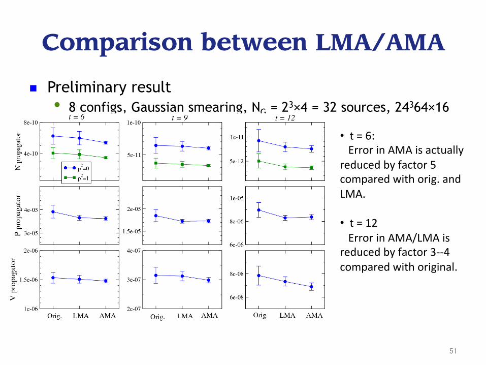
Comparison between LMA/AMA

n  Preliminary result •  8 configs, Gaussian smearing, NG = 23×4 = 32 sources, 24364×16

DWF •  t = 6: Error in AMA is actually reduced by factor 5 compared with orig. and LMA. •  t = 12 Error in AMA/LMA is reduced by factor 3-‐-‐4 compared with original.

51

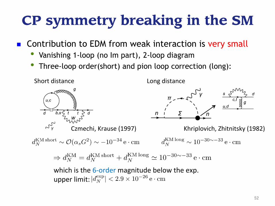
n  Contribution to EDM from weak interaction is very small •  Vanishing 1-loop (no Im part), 2-loop diagram •  Three-loop order(short) and pion loop correction (long):

CP symmetry breaking in the SM

Czmechi, Krause (1997) Khriplovich, Zhitnitsky (1982)

Short distance Long distance

which is the 6-‐order magnitude below the exp. upper limit:

52

Lattice-QCD calculations for EDMs - INDICO-FNAL (Indico)

Documents

Transcript of Lattice-QCD calculations for EDMs - INDICO-FNAL (Indico)