
Title of slide - CERN Indico
54
G. Cowan CERN Academic Training 2010 / Statistics for the LHC / Lecture 1 1 Statistics for the LHC Lecture 1: Introduction Academic Training Lectures CERN, 14–17 June, 2010 Glen Cowan Physics Department Royal Holloway, University of London [email protected] www.pp.rhul.ac.uk/~cowan indico.cern.ch/conferenceDisplay.py?confId=77830
-
Upload
khangminh22 -
Category
Documents
-
view
2 -
download
0
Transcript of Title of slide - CERN Indico
G. Cowan CERN Academic Training 2010 / Statistics for the LHC / Lecture 1 1
Statistics for the LHCLecture 1: Introduction
Academic Training Lectures
CERN, 14–17 June, 2010
Glen Cowan
Physics Department
Royal Holloway, University of [email protected]
www.pp.rhul.ac.uk/~cowan
indico.cern.ch/conferenceDisplay.py?confId=77830
G. Cowan CERN Academic Training 2010 / Statistics for the LHC / Lecture 1 2
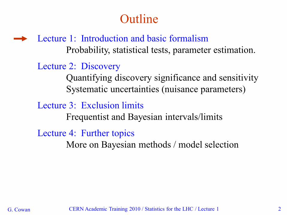
Outline
Lecture 1: Introduction and basic formalism
Probability, statistical tests, parameter estimation.
Lecture 2: Discovery
Quantifying discovery significance and sensitivity
Systematic uncertainties (nuisance parameters)
Lecture 3: Exclusion limits
Frequentist and Bayesian intervals/limits
Lecture 4: Further topics
More on Bayesian methods / model selection
G. Cowan CERN Academic Training 2010 / Statistics for the LHC / Lecture 1 3
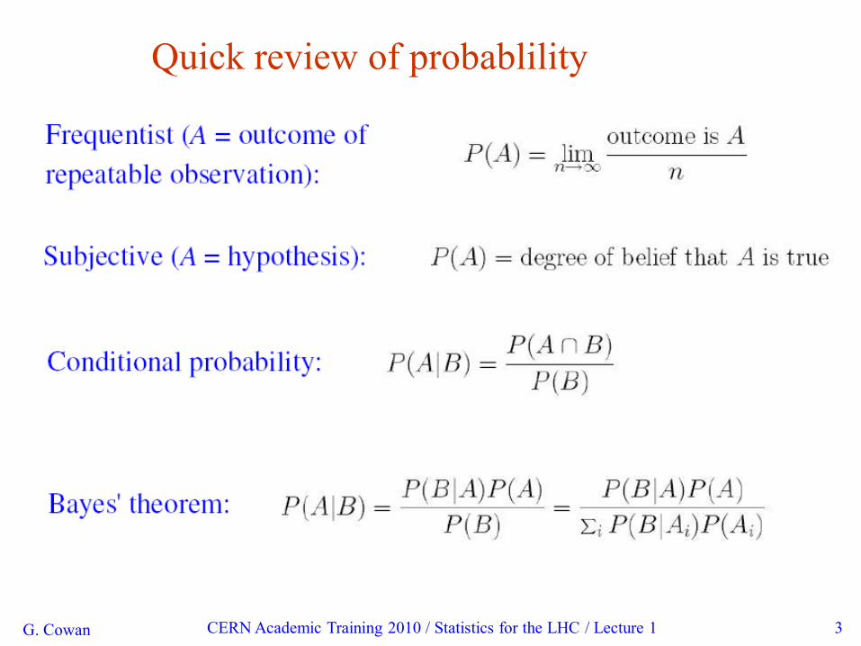
Quick review of probablility
G. Cowan CERN Academic Training 2010 / Statistics for the LHC / Lecture 1 4
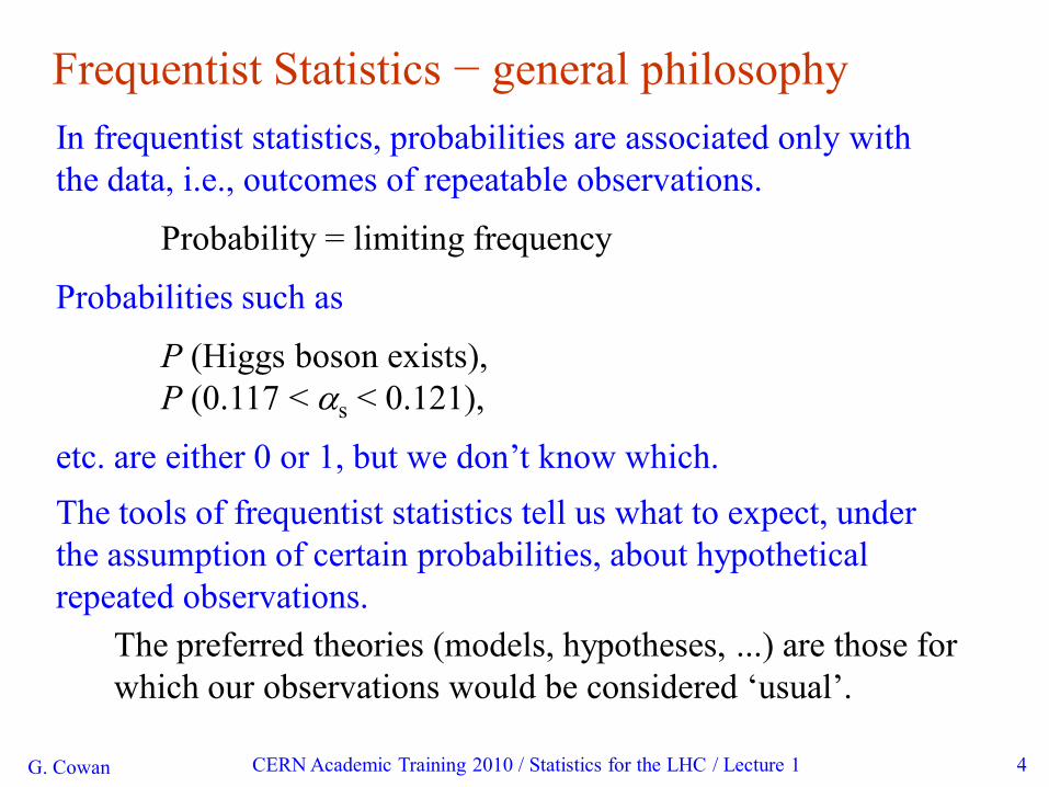
Frequentist Statistics − general philosophy
In frequentist statistics, probabilities are associated only with
the data, i.e., outcomes of repeatable observations.
Probability = limiting frequency
Probabilities such as
P (Higgs boson exists),
P (0.117 < as < 0.121),
etc. are either 0 or 1, but we don‟t know which.
The tools of frequentist statistics tell us what to expect, under
the assumption of certain probabilities, about hypothetical
repeated observations.
The preferred theories (models, hypotheses, ...) are those for
which our observations would be considered „usual‟.
G. Cowan CERN Academic Training 2010 / Statistics for the LHC / Lecture 1 5
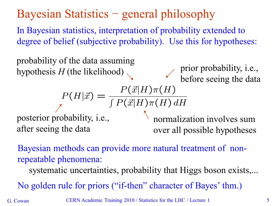
Bayesian Statistics − general philosophy
In Bayesian statistics, interpretation of probability extended to
degree of belief (subjective probability). Use this for hypotheses:
posterior probability, i.e.,
after seeing the data
prior probability, i.e.,
before seeing the data
probability of the data assuming
hypothesis H (the likelihood)
normalization involves sum
over all possible hypotheses
Bayesian methods can provide more natural treatment of non-
repeatable phenomena:
systematic uncertainties, probability that Higgs boson exists,...
No golden rule for priors (“if-then” character of Bayes‟ thm.)
G. Cowan CERN Academic Training 2010 / Statistics for the LHC / Lecture 1 6
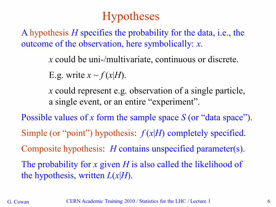
Hypotheses
A hypothesis H specifies the probability for the data, i.e., the
outcome of the observation, here symbolically: x.
x could be uni-/multivariate, continuous or discrete.
E.g. write x ~ f (x|H).
x could represent e.g. observation of a single particle,
a single event, or an entire “experiment”.
Possible values of x form the sample space S (or “data space”).
Simple (or “point”) hypothesis: f (x|H) completely specified.
Composite hypothesis: H contains unspecified parameter(s).
The probability for x given H is also called the likelihood of
the hypothesis, written L(x|H).
G. Cowan CERN Academic Training 2010 / Statistics for the LHC / Lecture 1 7
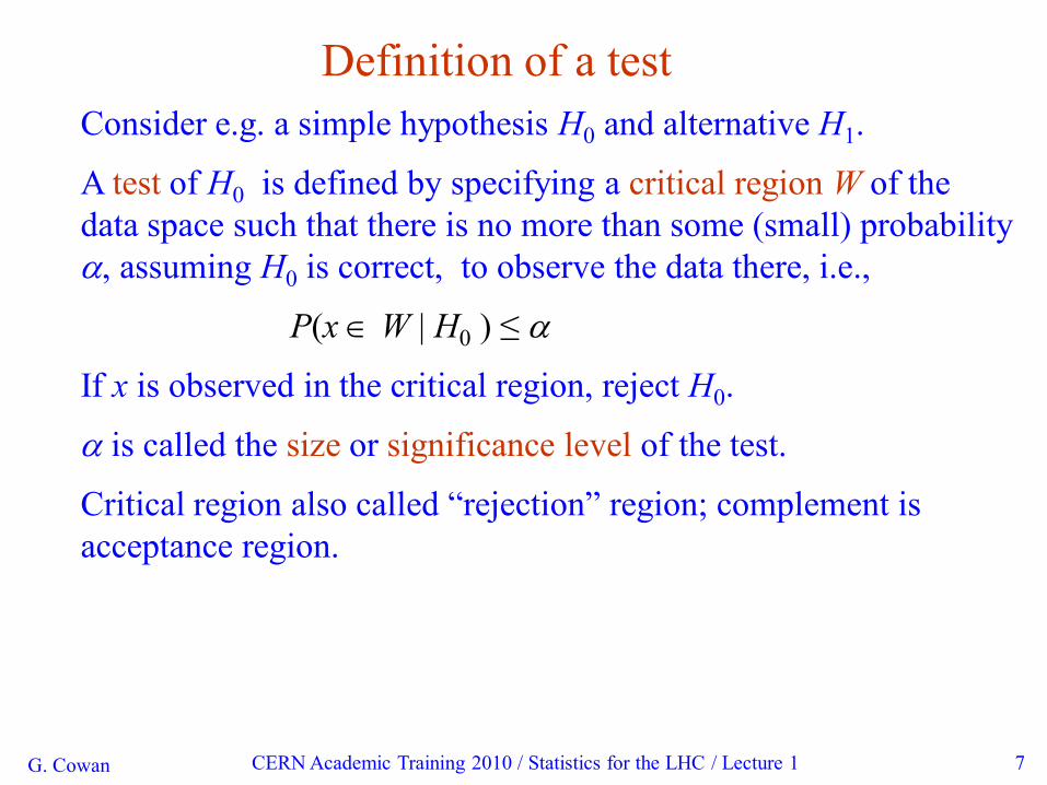
Definition of a test
Consider e.g. a simple hypothesis H0 and alternative H1.
A test of H0 is defined by specifying a critical region W of the
data space such that there is no more than some (small) probability
a, assuming H0 is correct, to observe the data there, i.e.,
P(x W | H0 ) ≤ a
If x is observed in the critical region, reject H0.
a is called the size or significance level of the test.
Critical region also called “rejection” region; complement is
acceptance region.
G. Cowan CERN Academic Training 2010 / Statistics for the LHC / Lecture 1 8
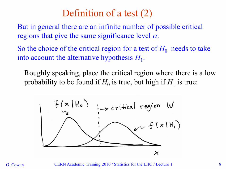
Definition of a test (2)
But in general there are an infinite number of possible critical
regions that give the same significance level a.
So the choice of the critical region for a test of H0 needs to take
into account the alternative hypothesis H1.
Roughly speaking, place the critical region where there is a low
probability to be found if H0 is true, but high if H1 is true:
G. Cowan CERN Academic Training 2010 / Statistics for the LHC / Lecture 1 9
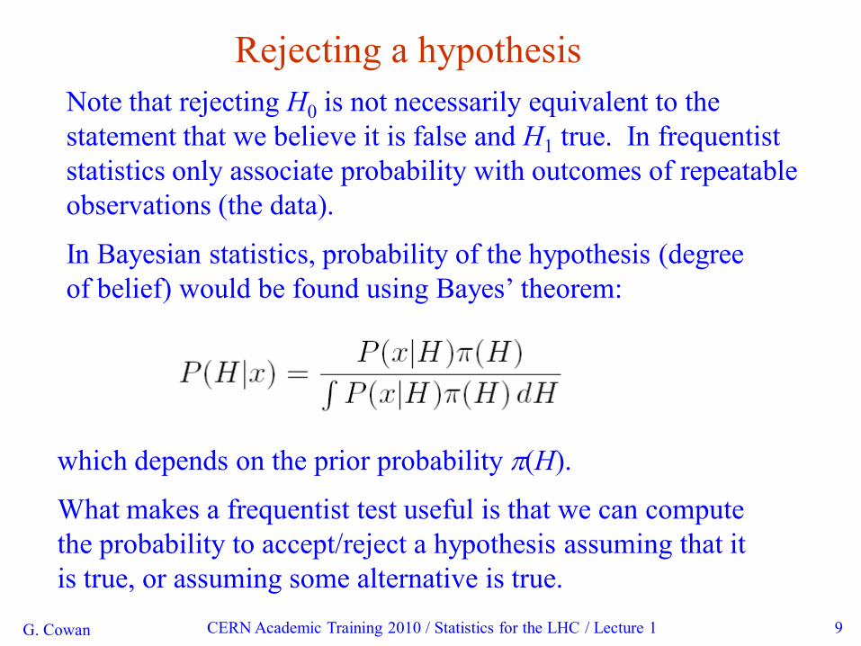
Rejecting a hypothesis
Note that rejecting H0 is not necessarily equivalent to the
statement that we believe it is false and H1 true. In frequentist
statistics only associate probability with outcomes of repeatable
observations (the data).
In Bayesian statistics, probability of the hypothesis (degree
of belief) would be found using Bayes‟ theorem:
which depends on the prior probability p(H).
What makes a frequentist test useful is that we can compute
the probability to accept/reject a hypothesis assuming that it
is true, or assuming some alternative is true.
G. Cowan CERN Academic Training 2010 / Statistics for the LHC / Lecture 1 10
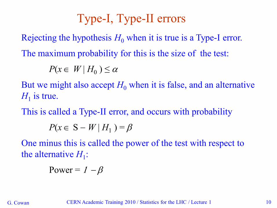
Type-I, Type-II errors
Rejecting the hypothesis H0 when it is true is a Type-I error.
The maximum probability for this is the size of the test:
P(x W | H0 ) ≤ a
But we might also accept H0 when it is false, and an alternative
H1 is true.
This is called a Type-II error, and occurs with probability
P(x S - W | H1 ) = b
One minus this is called the power of the test with respect to
the alternative H1:
Power = 1 - b
G. Cowan CERN Academic Training 2010 / Statistics for the LHC / Lecture 1 11
Physics context of a statistical test
Event Selection: the event types in question are both known to exist.
Example: separation of different particle types (electron vs muon)
or known event types (ttbar vs QCD multijet).
Use the selected sample for further study.
Search for New Physics: the null hypothesis H0 means Standard Model
events, and the alternative H1 means "events of a type whose existence
is not yet established" (to establish or exclude the signal model is the goal
of the analysis).
Many subtle issues here, mainly related to the heavy burden
of proof required to establish presence of a new phenomenon.
The optimal statistical test for a search is closely related to that used for
event selection.
G. Cowan CERN Academic Training 2010 / Statistics for the LHC / Lecture 1 12
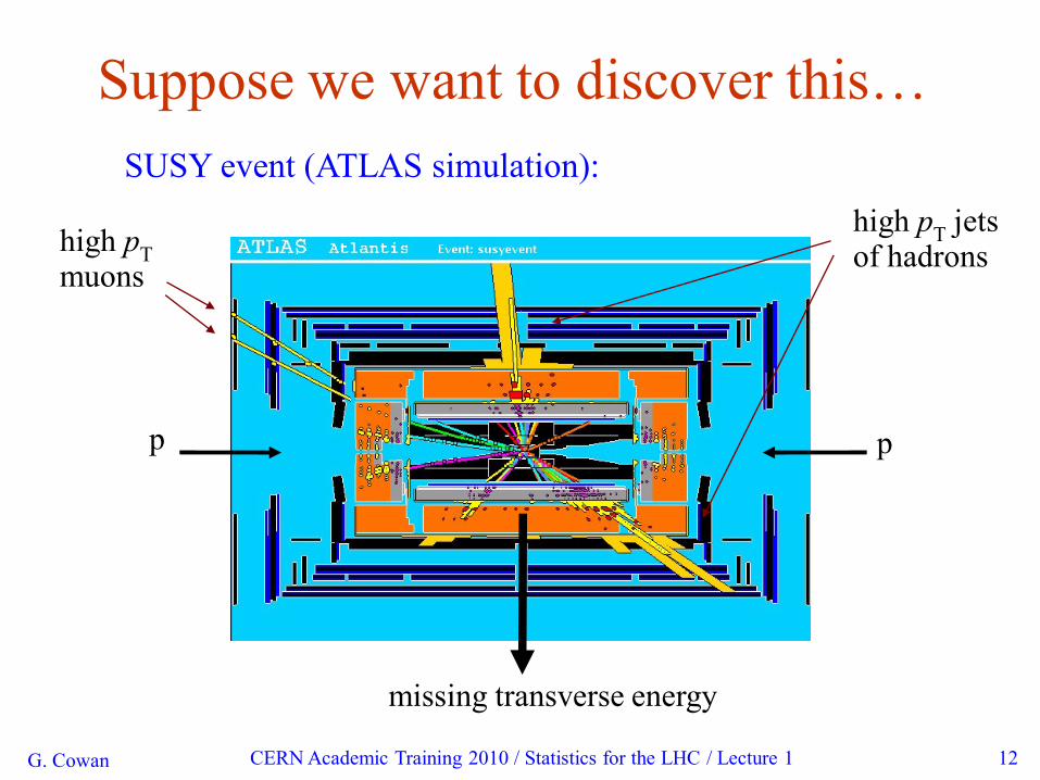
Suppose we want to discover this…
high pT
muons
high pT
jets of hadrons
missing transverse energy
p p
SUSY event (ATLAS simulation):
G. Cowan CERN Academic Training 2010 / Statistics for the LHC / Lecture 1 13
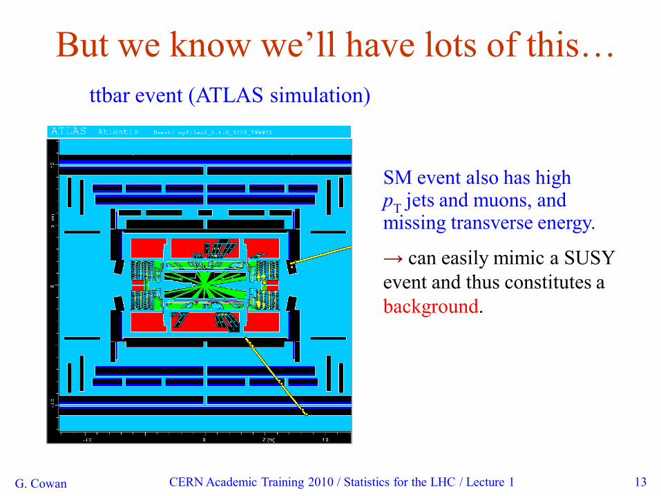
But we know we‟ll have lots of this…
SM event also has high p
Tjets and muons, and
missing transverse energy.
→ can easily mimic a SUSY
event and thus constitutes a
background.
ttbar event (ATLAS simulation)
G. Cowan CERN Academic Training 2010 / Statistics for the LHC / Lecture 1 14
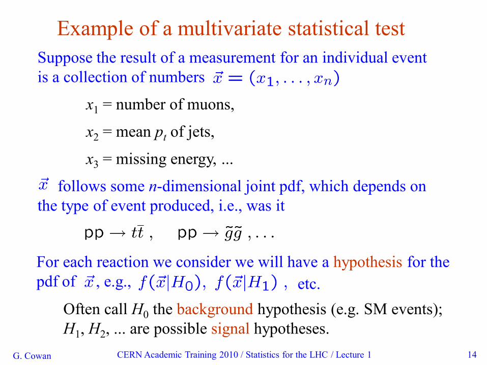
For each reaction we consider we will have a hypothesis for the
pdf of , e.g.,
Example of a multivariate statistical test
Suppose the result of a measurement for an individual event
is a collection of numbers
x1 = number of muons,
x2 = mean pt of jets,
x3 = missing energy, ...
follows some n-dimensional joint pdf, which depends on
the type of event produced, i.e., was it
etc.
Often call H0 the background hypothesis (e.g. SM events);
H1, H2, ... are possible signal hypotheses.
G. Cowan CERN Academic Training 2010 / Statistics for the LHC / Lecture 1 15
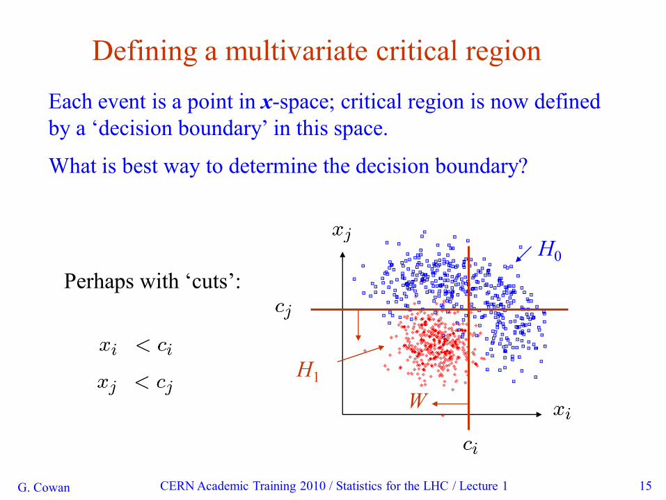
Defining a multivariate critical region
Each event is a point in x-space; critical region is now defined
by a „decision boundary‟ in this space.
What is best way to determine the decision boundary?
W
H1
H0
Perhaps with „cuts‟:
G. Cowan CERN Academic Training 2010 / Statistics for the LHC / Lecture 1 16
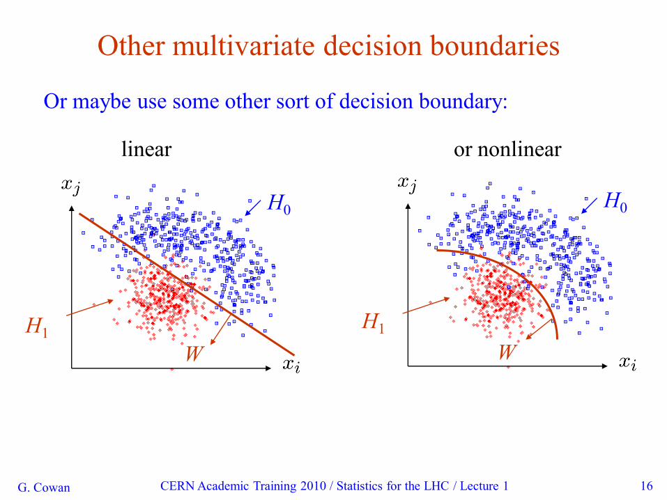
Other multivariate decision boundaries
Or maybe use some other sort of decision boundary:
W
H1
H0
W
H1
H0
linear or nonlinear
G. Cowan CERN Academic Training 2010 / Statistics for the LHC / Lecture 1 Lecture 1 page 17
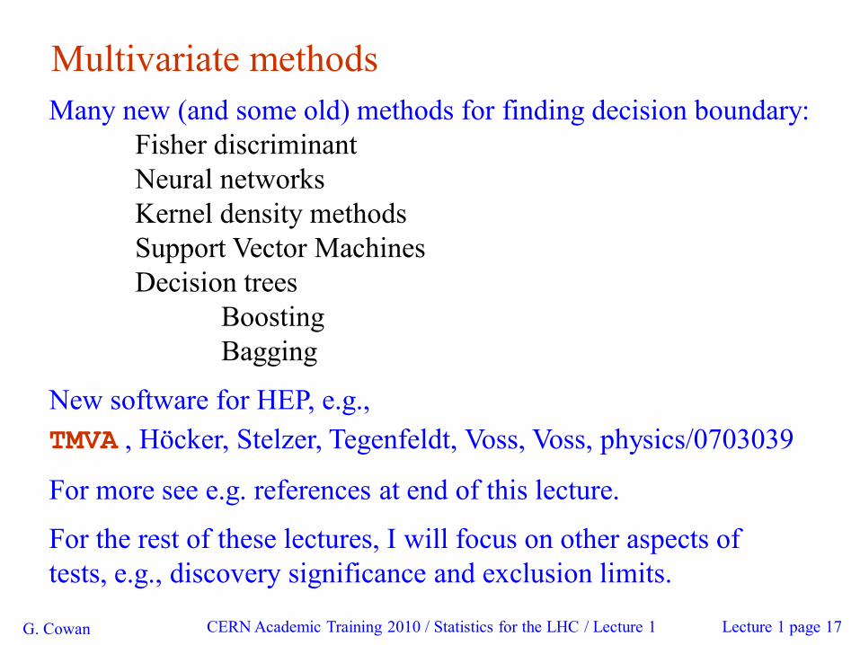
Multivariate methods
Many new (and some old) methods for finding decision boundary:
Fisher discriminant
Neural networks
Kernel density methods
Support Vector Machines
Decision trees
Boosting
Bagging
New software for HEP, e.g.,
TMVA , Höcker, Stelzer, Tegenfeldt, Voss, Voss, physics/0703039
For more see e.g. references at end of this lecture.
For the rest of these lectures, I will focus on other aspects of
tests, e.g., discovery significance and exclusion limits.
G. Cowan CERN Academic Training 2010 / Statistics for the LHC / Lecture 1 18
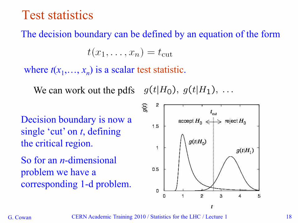
Test statistics
The decision boundary can be defined by an equation of the form
We can work out the pdfs
Decision boundary is now a
single „cut‟ on t, defining
the critical region.
So for an n-dimensional
problem we have a
corresponding 1-d problem.
where t(x1,…, xn) is a scalar test statistic.
G. Cowan CERN Academic Training 2010 / Statistics for the LHC / Lecture 1 19
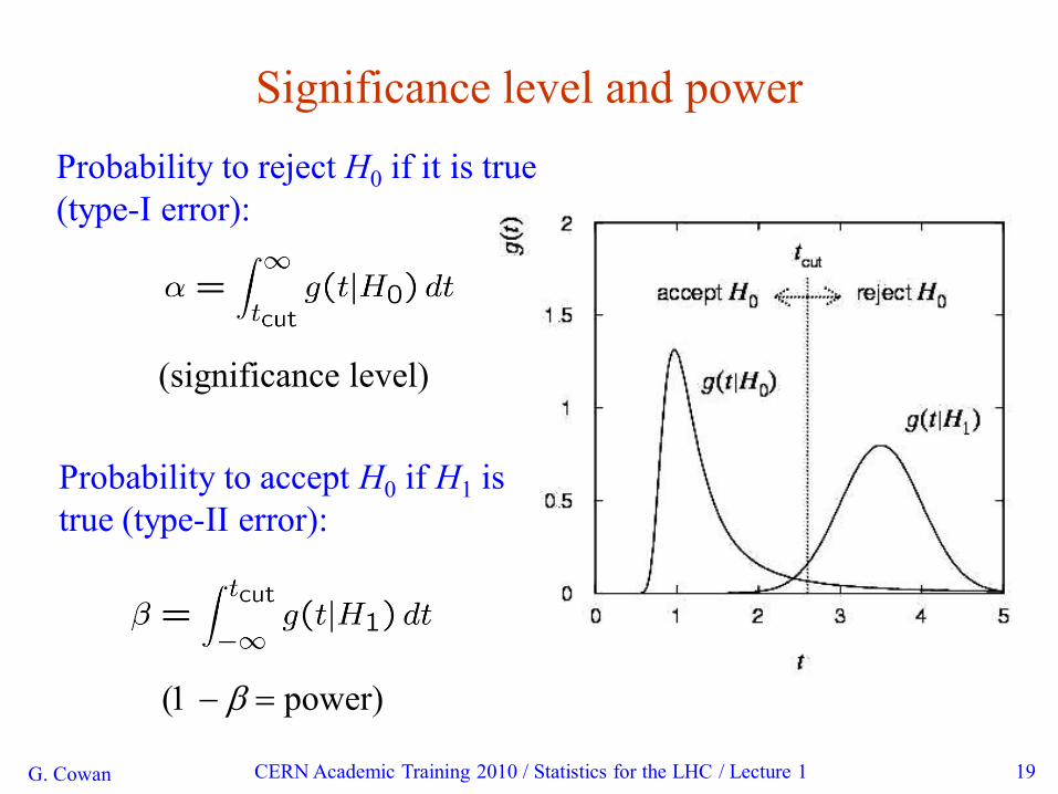
Significance level and power
Probability to reject H0 if it is true
(type-I error):
(significance level)
Probability to accept H0 if H1 is
true (type-II error):
(1 - b = power)
G. Cowan CERN Academic Training 2010 / Statistics for the LHC / Lecture 1 20
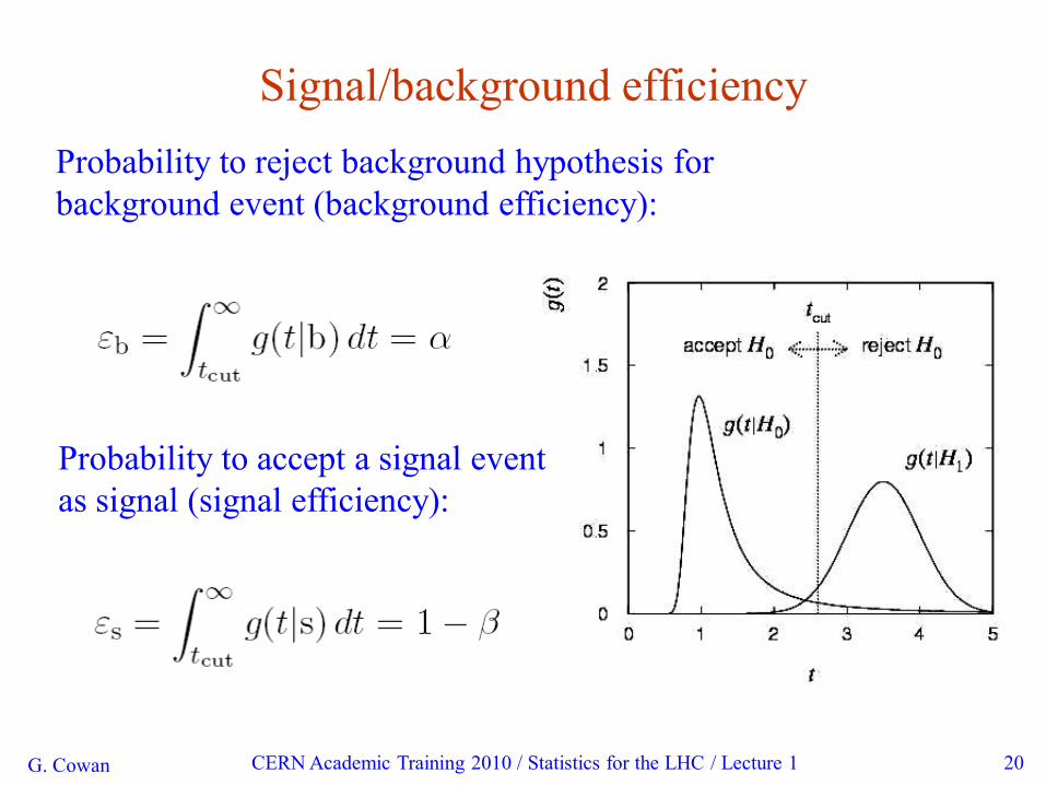
Signal/background efficiency
Probability to reject background hypothesis for
background event (background efficiency):
Probability to accept a signal event
as signal (signal efficiency):
G. Cowan CERN Academic Training 2010 / Statistics for the LHC / Lecture 1 21
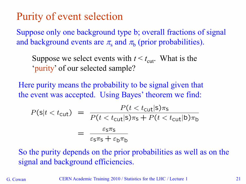
Purity of event selection
Suppose only one background type b; overall fractions of signal
and background events are ps and pb (prior probabilities).
Suppose we select events with t < tcut. What is the
„purity‟ of our selected sample?
Here purity means the probability to be signal given that
the event was accepted. Using Bayes‟ theorem we find:
So the purity depends on the prior probabilities as well as on the
signal and background efficiencies.
G. Cowan CERN Academic Training 2010 / Statistics for the LHC / Lecture 1 22
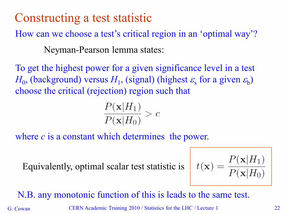
Constructing a test statistic
How can we choose a test‟s critical region in an „optimal way‟?
Neyman-Pearson lemma states:
To get the highest power for a given significance level in a test
H0, (background) versus H1, (signal) (highest es for a given eb)
choose the critical (rejection) region such that
where c is a constant which determines the power.
Equivalently, optimal scalar test statistic is
N.B. any monotonic function of this is leads to the same test.
G. Cowan CERN Academic Training 2010 / Statistics for the LHC / Lecture 1 23
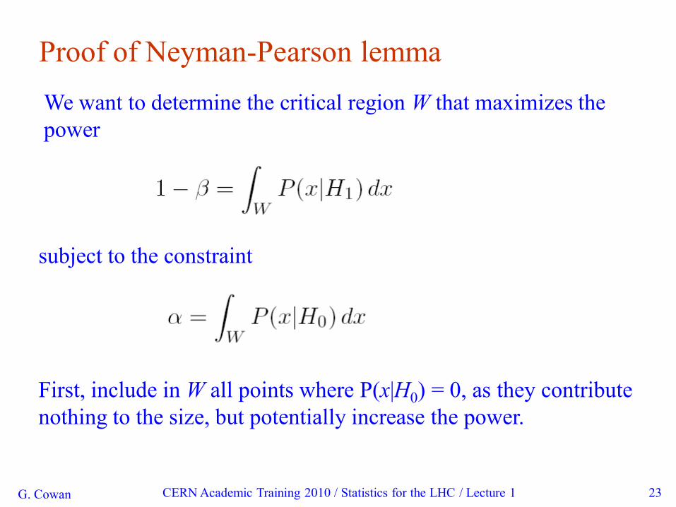
Proof of Neyman-Pearson lemma
We want to determine the critical region W that maximizes the
power
subject to the constraint
First, include in W all points where P(x|H0) = 0, as they contribute
nothing to the size, but potentially increase the power.
G. Cowan CERN Academic Training 2010 / Statistics for the LHC / Lecture 1 24
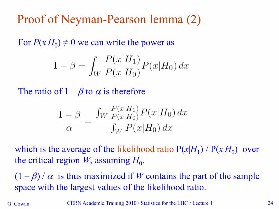
Proof of Neyman-Pearson lemma (2)
For P(x|H0) ≠ 0 we can write the power as
The ratio of 1 – b to a is therefore
which is the average of the likelihood ratio P(x|H1) / P(x|H0) over
the critical region W, assuming H0.
(1 – b) / a is thus maximized if W contains the part of the sample
space with the largest values of the likelihood ratio.

G. Cowan CERN Academic Training 2010 / Statistics for the LHC / Lecture 1 25
Testing significance / goodness-of-fit
Suppose hypothesis H predicts pdf
observations
for a set of
We observe a single point in this space:
What can we say about the validity of H in light of the data?
Decide what part of the
data space represents less
compatibility with H than
does the point less
compatible
with H
more
compatible
with H
(Not unique!)
G. Cowan CERN Academic Training 2010 / Statistics for the LHC / Lecture 1 26
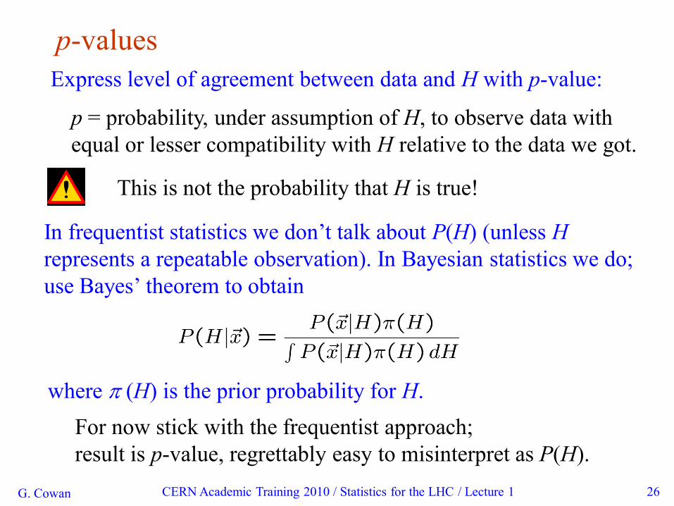
p-values
where p (H) is the prior probability for H.
Express level of agreement between data and H with p-value:
p = probability, under assumption of H, to observe data with
equal or lesser compatibility with H relative to the data we got.
This is not the probability that H is true!
In frequentist statistics we don‟t talk about P(H) (unless H
represents a repeatable observation). In Bayesian statistics we do;
use Bayes‟ theorem to obtain
For now stick with the frequentist approach;
result is p-value, regrettably easy to misinterpret as P(H).
G. Cowan 27
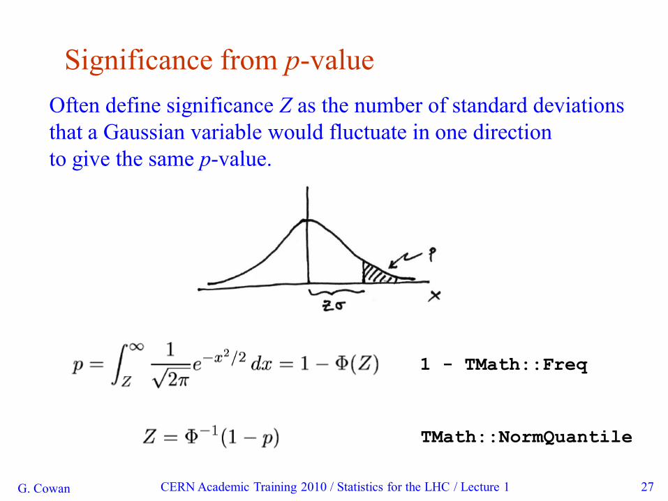
Significance from p-value
Often define significance Z as the number of standard deviations
that a Gaussian variable would fluctuate in one direction
to give the same p-value.
1 - TMath::Freq
TMath::NormQuantile
CERN Academic Training 2010 / Statistics for the LHC / Lecture 1
G. Cowan CERN Academic Training 2010 / Statistics for the LHC / Lecture 1 28
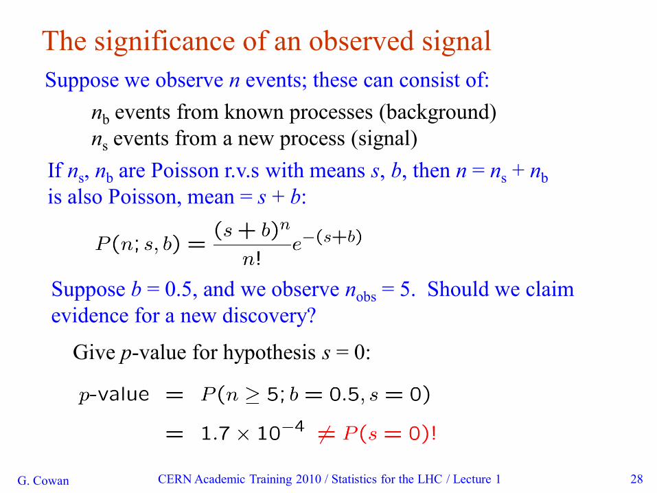
The significance of an observed signal
Suppose we observe n events; these can consist of:
nb events from known processes (background)
ns events from a new process (signal)
If ns, nb are Poisson r.v.s with means s, b, then n = ns + nb
is also Poisson, mean = s + b:
Suppose b = 0.5, and we observe nobs = 5. Should we claim
evidence for a new discovery?
Give p-value for hypothesis s = 0:
G. Cowan page 29
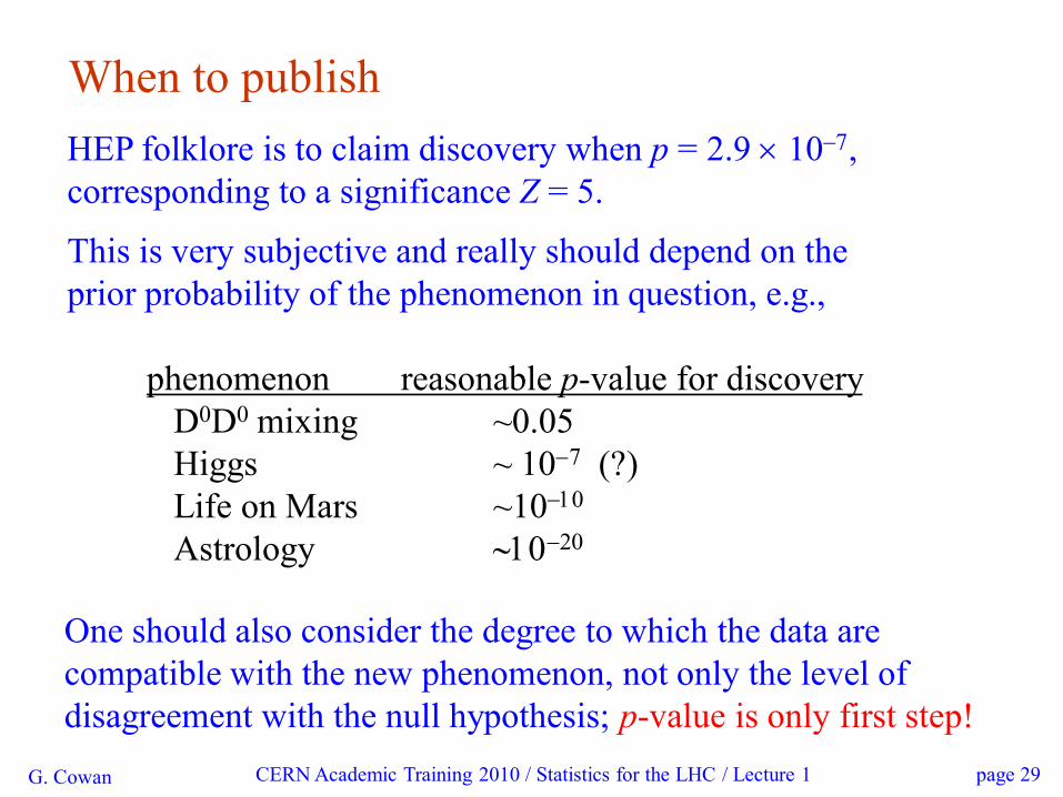
When to publish
HEP folklore is to claim discovery when p = 2.9 10-7,
corresponding to a significance Z = 5.
This is very subjective and really should depend on the
prior probability of the phenomenon in question, e.g.,
phenomenon reasonable p-value for discovery
D0D0 mixing ~0.05
Higgs ~ 10-7 (?)
Life on Mars ~10-10
Astrology ~10-20
One should also consider the degree to which the data are
compatible with the new phenomenon, not only the level of
disagreement with the null hypothesis; p-value is only first step!
CERN Academic Training 2010 / Statistics for the LHC / Lecture 1
G. Cowan page 30
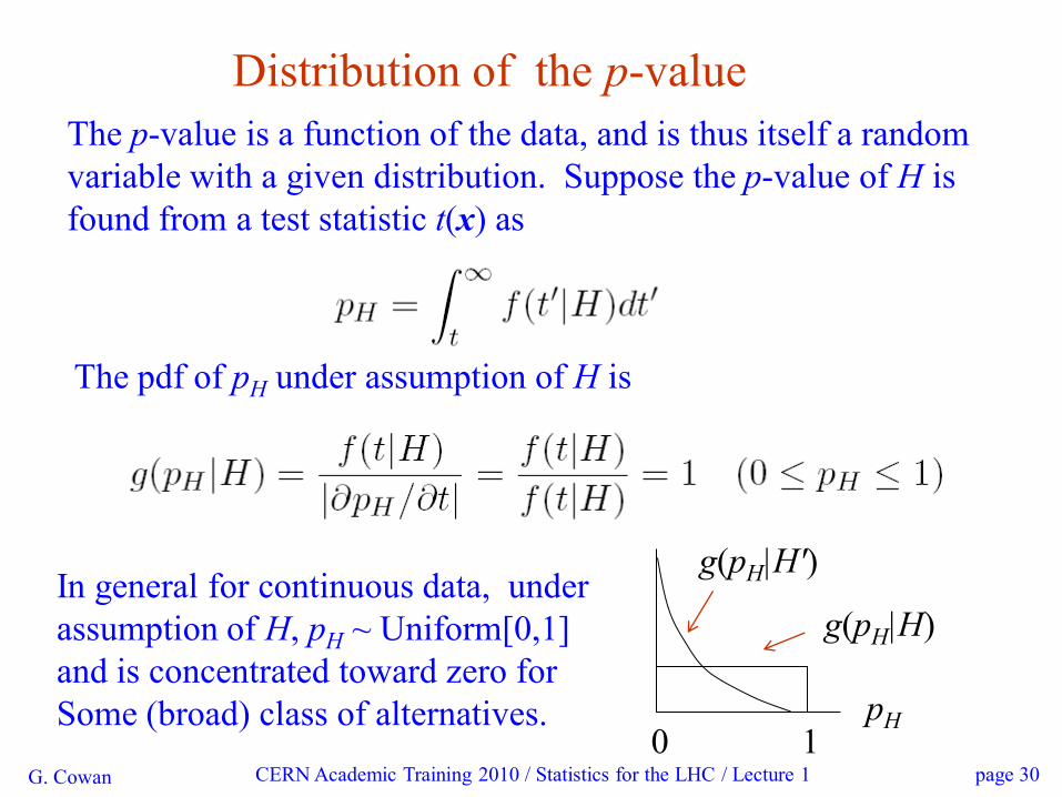
Distribution of the p-value
The p-value is a function of the data, and is thus itself a random
variable with a given distribution. Suppose the p-value of H is
found from a test statistic t(x) as
CERN Academic Training 2010 / Statistics for the LHC / Lecture 1
The pdf of pH under assumption of H is
In general for continuous data, under
assumption of H, pH ~ Uniform[0,1]
and is concentrated toward zero for
Some (broad) class of alternatives. pH
g(pH|H)
0 1
g(pH|H′)
G. Cowan page 31
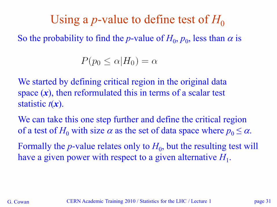
Using a p-value to define test of H0
So the probability to find the p-value of H0, p0, less than a is
CERN Academic Training 2010 / Statistics for the LHC / Lecture 1
We started by defining critical region in the original data
space (x), then reformulated this in terms of a scalar test
statistic t(x).
We can take this one step further and define the critical region
of a test of H0 with size a as the set of data space where p0 ≤ a.
Formally the p-value relates only to H0, but the resulting test will
have a given power with respect to a given alternative H1.
G. Cowan CERN Academic Training 2010 / Statistics for the LHC / Lecture 1 32
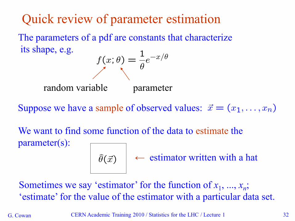
Quick review of parameter estimation
The parameters of a pdf are constants that characterize
its shape, e.g.
random variable
Suppose we have a sample of observed values:
parameter
We want to find some function of the data to estimate the
parameter(s):
← estimator written with a hat
Sometimes we say „estimator‟ for the function of x1, ..., xn;
„estimate‟ for the value of the estimator with a particular data set.
G. Cowan CERN Academic Training 2010 / Statistics for the LHC / Lecture 1 33
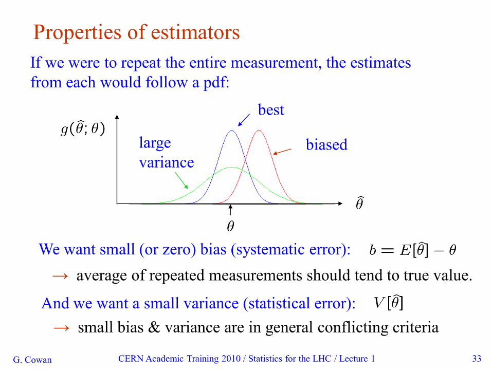
Properties of estimators
If we were to repeat the entire measurement, the estimates
from each would follow a pdf:
biasedlarge
variance
best
We want small (or zero) bias (systematic error):
→ average of repeated measurements should tend to true value.
And we want a small variance (statistical error):
→ small bias & variance are in general conflicting criteria
G. Cowan CERN Academic Training 2010 / Statistics for the LHC / Lecture 1 34
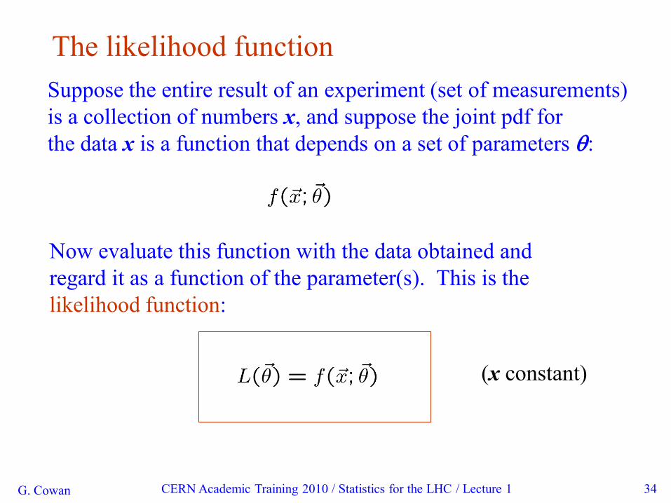
The likelihood function
Suppose the entire result of an experiment (set of measurements)
is a collection of numbers x, and suppose the joint pdf for
the data x is a function that depends on a set of parameters q:
Now evaluate this function with the data obtained and
regard it as a function of the parameter(s). This is the
likelihood function:
(x constant)
G. Cowan CERN Academic Training 2010 / Statistics for the LHC / Lecture 1 35
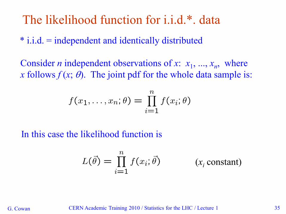
The likelihood function for i.i.d.*. data
Consider n independent observations of x: x1, ..., xn, where
x follows f (x; q). The joint pdf for the whole data sample is:
In this case the likelihood function is
(xi constant)
* i.i.d. = independent and identically distributed
G. Cowan CERN Academic Training 2010 / Statistics for the LHC / Lecture 1 36
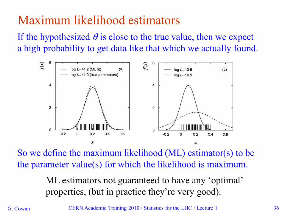
Maximum likelihood estimators
If the hypothesized q is close to the true value, then we expect
a high probability to get data like that which we actually found.
So we define the maximum likelihood (ML) estimator(s) to be
the parameter value(s) for which the likelihood is maximum.
ML estimators not guaranteed to have any „optimal‟
properties, (but in practice they‟re very good).
G. Cowan CERN Academic Training 2010 / Statistics for the LHC / Lecture 1 37
Wrapping up lecture 1
General framework of a statistical test:
Divide data spaced into two regions; depending on
where data are then observed, accept or reject hypothesis.
Properties:
significance level (rate of Type-I error)
power (one minus rate of Type-II error)
Significance tests (also for goodness-of-fit):
p-value = probability to see level of incompatibility
between data and hypothesis equal to or greater than
level found with the actual data.
Parameter estimation
Maximize likelihood function → ML estimator

G. Cowan CERN Academic Training 2010 / Statistics for the LHC / Lecture 1 38
Extra slides
G. Cowan CERN Academic Training 2010 / Statistics for the LHC / Lecture 1 39
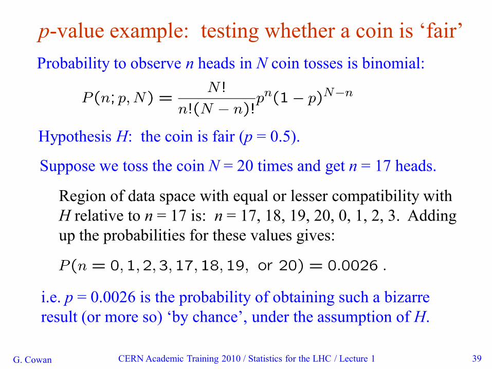
p-value example: testing whether a coin is „fair‟
i.e. p = 0.0026 is the probability of obtaining such a bizarre
result (or more so) „by chance‟, under the assumption of H.
Probability to observe n heads in N coin tosses is binomial:
Hypothesis H: the coin is fair (p = 0.5).
Suppose we toss the coin N = 20 times and get n = 17 heads.
Region of data space with equal or lesser compatibility with
H relative to n = 17 is: n = 17, 18, 19, 20, 0, 1, 2, 3. Adding
up the probabilities for these values gives:
G. Cowan CERN Academic Training 2010 / Statistics for the LHC / Lecture 1 40
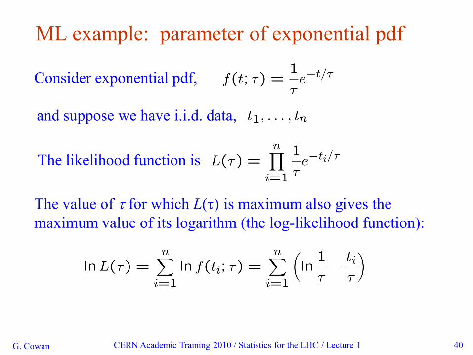
ML example: parameter of exponential pdf
Consider exponential pdf,
and suppose we have i.i.d. data,
The likelihood function is
The value of t for which L(t) is maximum also gives the
maximum value of its logarithm (the log-likelihood function):
G. Cowan CERN Academic Training 2010 / Statistics for the LHC / Lecture 1 41
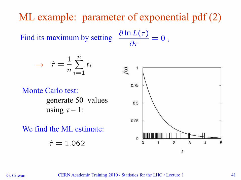
ML example: parameter of exponential pdf (2)
Find its maximum by setting
→
Monte Carlo test:
generate 50 values
using t = 1:
We find the ML estimate:
G. Cowan CERN Academic Training 2010 / Statistics for the LHC / Lecture 1 42
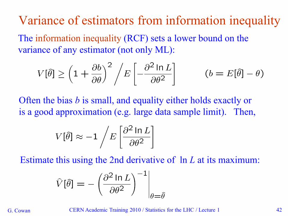
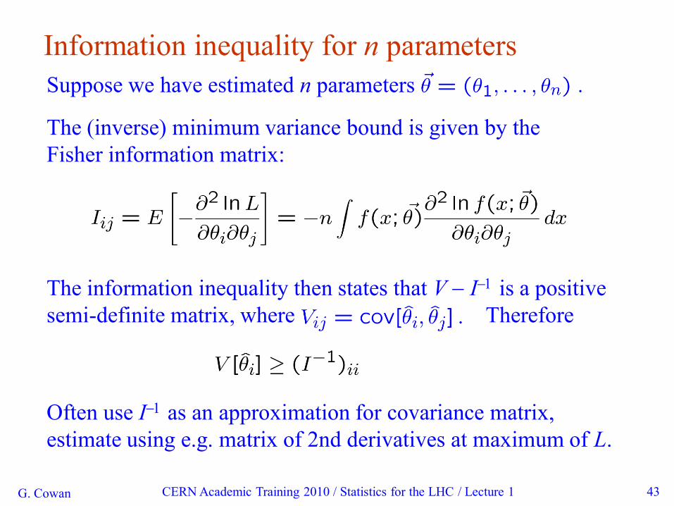
Variance of estimators from information inequality
The information inequality (RCF) sets a lower bound on the
variance of any estimator (not only ML):
Often the bias b is small, and equality either holds exactly or
is a good approximation (e.g. large data sample limit). Then,
Estimate this using the 2nd derivative of ln L at its maximum:
G. Cowan CERN Academic Training 2010 / Statistics for the LHC / Lecture 1 43
Information inequality for n parameters
Suppose we have estimated n parameters
The (inverse) minimum variance bound is given by the
Fisher information matrix:
The information inequality then states that V - I-1 is a positive
semi-definite matrix, where Therefore
Often use I-1 as an approximation for covariance matrix,
estimate using e.g. matrix of 2nd derivatives at maximum of L.
G. Cowan CERN Academic Training 2010 / Statistics for the LHC / Lecture 1 44
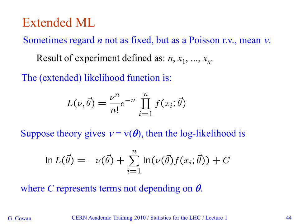
Extended ML
Sometimes regard n not as fixed, but as a Poisson r.v., mean n.
Result of experiment defined as: n, x1, ..., xn.
The (extended) likelihood function is:
Suppose theory gives n = n(q), then the log-likelihood is
where C represents terms not depending on q.
G. Cowan CERN Academic Training 2010 / Statistics for the LHC / Lecture 1 45
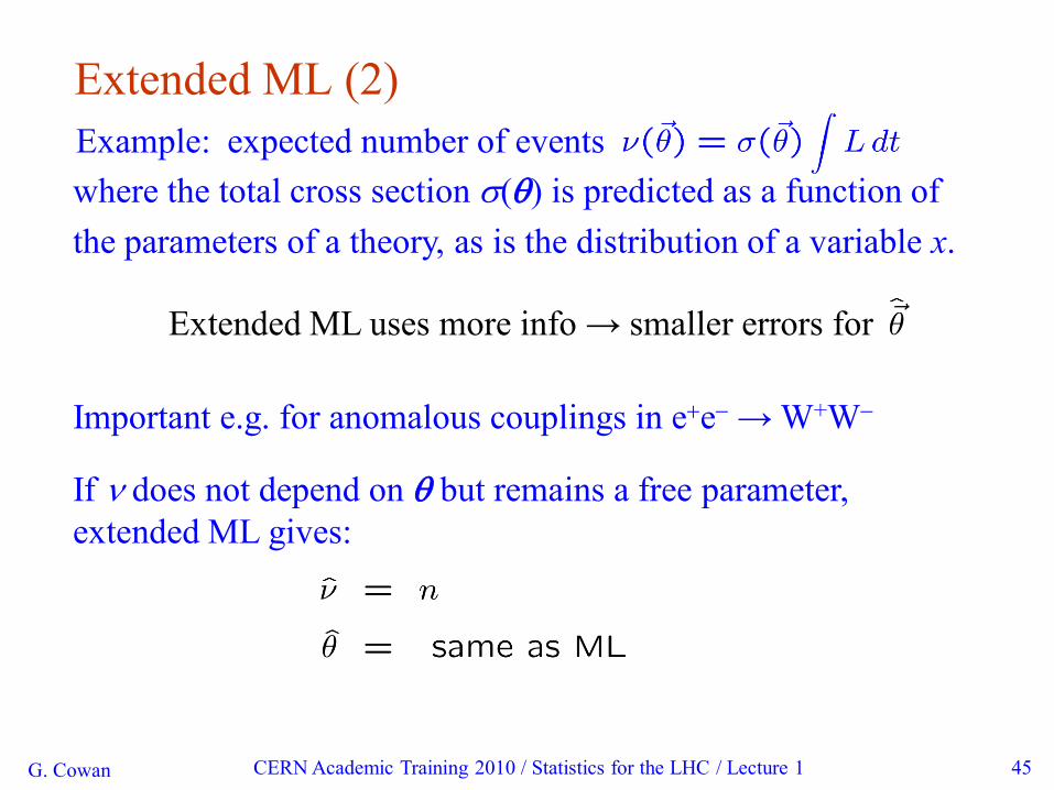
Extended ML (2)
Extended ML uses more info → smaller errors for
Example: expected number of events
where the total cross section s(q) is predicted as a function of
the parameters of a theory, as is the distribution of a variable x.
If n does not depend on q but remains a free parameter,
extended ML gives:
Important e.g. for anomalous couplings in e+e- → W+W-
G. Cowan CERN Academic Training 2010 / Statistics for the LHC / Lecture 1 46
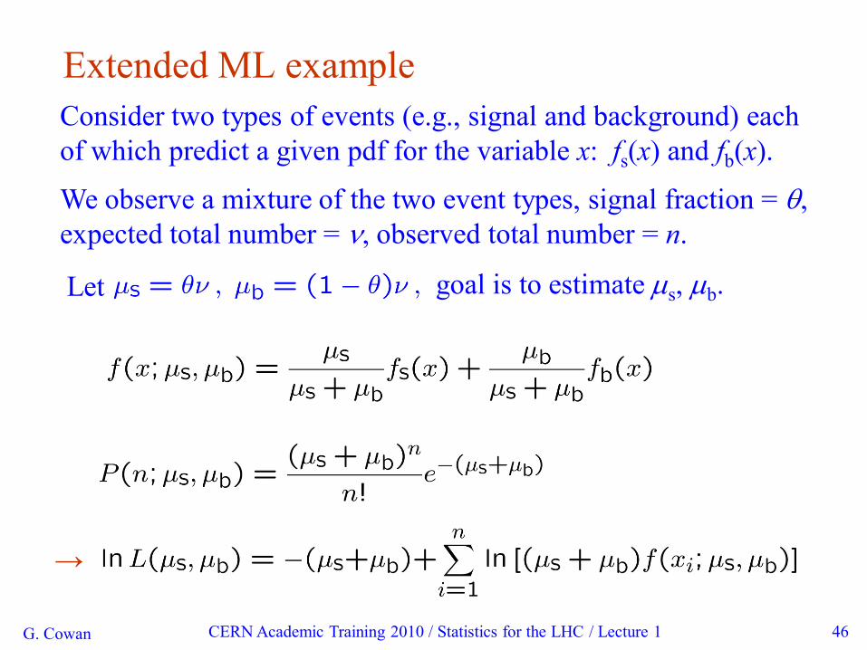
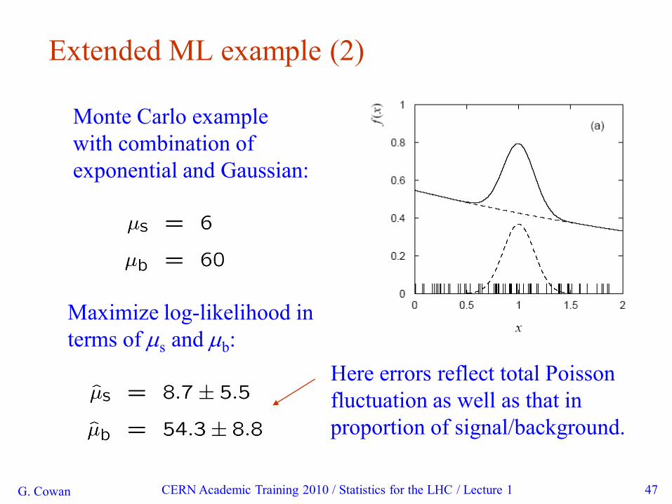
Extended ML example
Consider two types of events (e.g., signal and background) each
of which predict a given pdf for the variable x: fs(x) and fb(x).
We observe a mixture of the two event types, signal fraction = q,
expected total number = n, observed total number = n.
Let goal is to estimate ms, mb.
→
G. Cowan CERN Academic Training 2010 / Statistics for the LHC / Lecture 1 47
Extended ML example (2)
Maximize log-likelihood in
terms of ms and mb:
Monte Carlo example
with combination of
exponential and Gaussian:
Here errors reflect total Poisson
fluctuation as well as that in
proportion of signal/background.

G. Cowan CERN Academic Training 2010 / Statistics for the LHC / Lecture 1 48
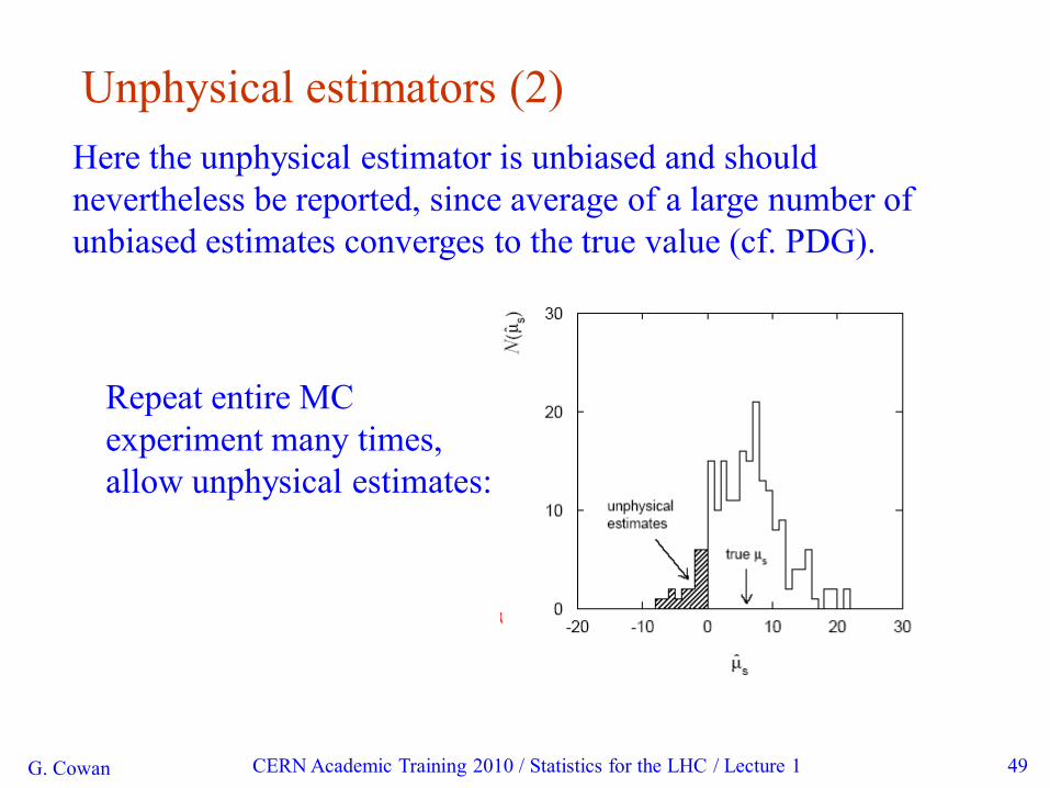
Extended ML example: an unphysical estimate
A downwards fluctuation of data in the peak region can lead
to even fewer events than what would be obtained from
background alone.
Estimate for ms here pushed
negative (unphysical).
We can let this happen as
long as the (total) pdf stays
positive everywhere.
G. Cowan CERN Academic Training 2010 / Statistics for the LHC / Lecture 1 49
Unphysical estimators (2)
Here the unphysical estimator is unbiased and should
nevertheless be reported, since average of a large number of
unbiased estimates converges to the true value (cf. PDG).
Repeat entire MC
experiment many times,
allow unphysical estimates:
G. Cowan CERN Academic Training 2010 / Statistics for the LHC / Lecture 1 page 50
G. Cowan CERN Academic Training 2010 / Statistics for the LHC / Lecture 1 page 51
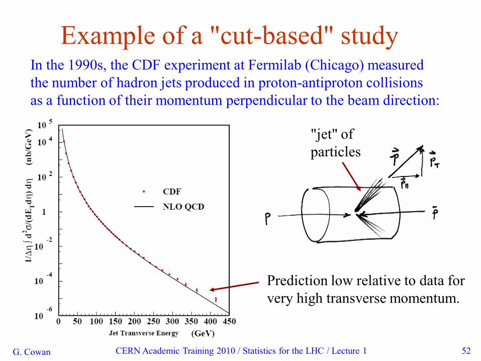
G. Cowan CERN Academic Training 2010 / Statistics for the LHC / Lecture 1 52
Example of a "cut-based" studyIn the 1990s, the CDF experiment at Fermilab (Chicago) measured
the number of hadron jets produced in proton-antiproton collisions
as a function of their momentum perpendicular to the beam direction:
Prediction low relative to data for
very high transverse momentum.
"jet" of
particles
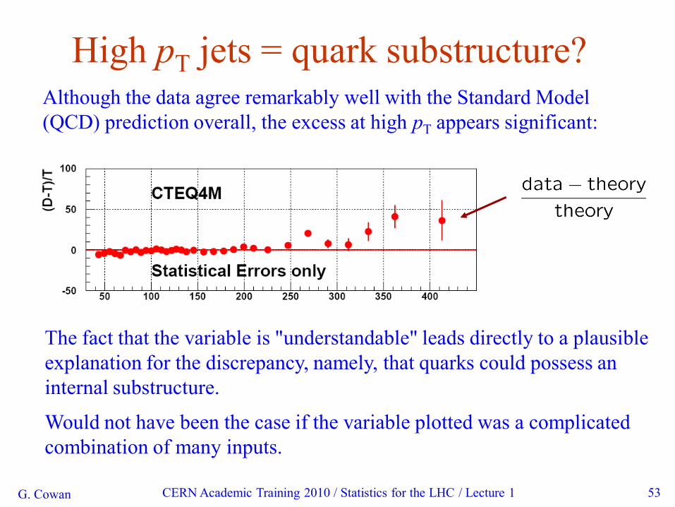
G. Cowan CERN Academic Training 2010 / Statistics for the LHC / Lecture 1 53
High pT jets = quark substructure?Although the data agree remarkably well with the Standard Model
(QCD) prediction overall, the excess at high pT appears significant:
The fact that the variable is "understandable" leads directly to a plausible
explanation for the discrepancy, namely, that quarks could possess an
internal substructure.
Would not have been the case if the variable plotted was a complicated
combination of many inputs.
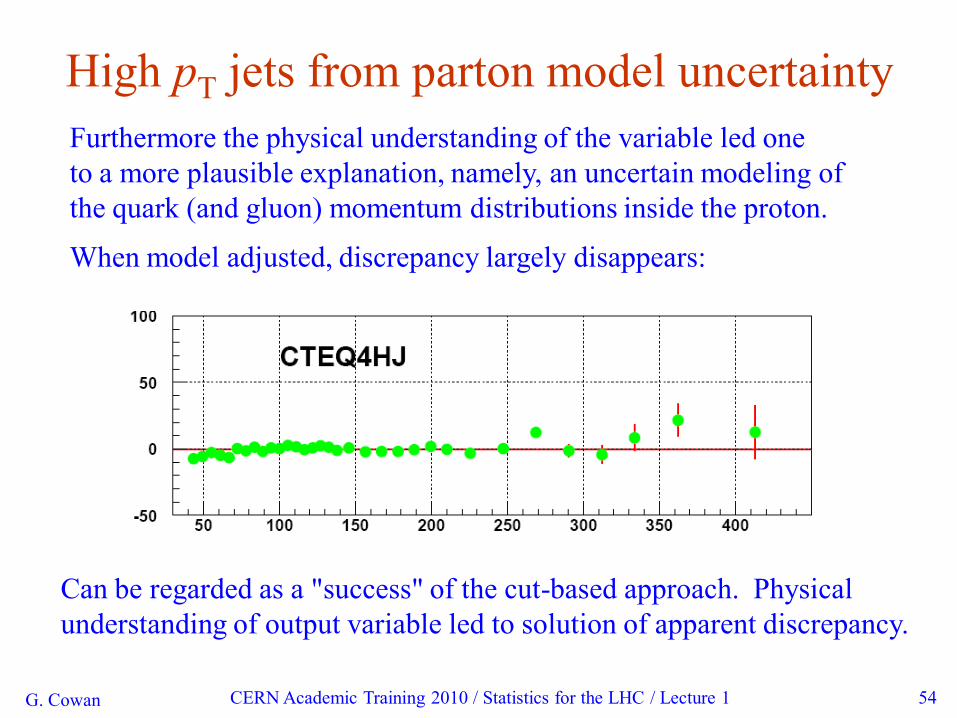
G. Cowan CERN Academic Training 2010 / Statistics for the LHC / Lecture 1 54
High pT jets from parton model uncertainty
Furthermore the physical understanding of the variable led one
to a more plausible explanation, namely, an uncertain modeling of
the quark (and gluon) momentum distributions inside the proton.
When model adjusted, discrepancy largely disappears:
Can be regarded as a "success" of the cut-based approach. Physical
understanding of output variable led to solution of apparent discrepancy.