arX

iv:0

708.

0207

v1 [

hep-

lat]

1 A

ug 2

007

UMD-40762-395

Restless pions: orbifold boundary conditions

and noise suppression in lattice QCD

Paulo F. Bedaque∗ and Andre Walker-Loud†

Maryland Center for Fundamental Physics

Department of Physics, University of Maryland, College Park, MD 20742

(Dated: February 1, 2008 - 17:37)

Abstract

The study of one or more baryons in lattice QCD is severely hindered by the exponential decay

in time of the signal-to-noise ratio. The rate at which the signal-to-noise decreases is a function

of the the pion mass. More precisely, it depends on the minimum allowed pion energy in the

box, which, for periodic boundary conditions, is equal to its mass. We propose a set of boundary

conditions, given by a “parity orbifold” construction, which eliminates the zero momentum pion

modes, raising the minimum pion energy without altering the QCD ground state, and thereby

improving the signal-to-noise ratio of (multi)-baryon correlation functions at long Euclidean times.

We discuss variations of these “restless pions” boundary conditions and focus on their impact on

the study of nuclear forces.

∗ bedaque@umd.edu† walkloud@umd.edu

1

I. INTRODUCTION

Lattice QCD studies of heavy systems are plagued by large statistical noise. The signal-

to-noise ratio of a correlation function created by an operator with n quark–anti-quark pairs

decreases with (Euclidean) time as e−(E−n2mπ)t, where E is the mass of the state under

consideration. This is a particularly nasty problem for the recent studies of nucleon-nucleon

[1, 2] and hyperon-nucleon [3] forces with lattice QCD. The large statistical error renders

the numerical information at large times useless. Compounded with this problem, at early

times the correlators are contaminated by excited states and so there is only a very narrow

range of time slices left containing useful information. In unquenched calculations [1, 3]

the statistical noise allows for semi-quantitative results only, even after the computation of

thousands of fermion propagators. These errors are also much larger than finite-volume [4]

and finite lattice spacing [5] effects in these observables.

We propose here a scheme to alleviate this signal-to-noise problem. We start with the

simple observation that the statistical noise is dominated by the energy of the lightest pion

states. Periodic boundary conditions allow a pion zero mode and thus the lowest pion

energy is equal to its mass. If one were to impose anti-periodic boundary conditions for all

three pions, then the pion zero-modes are forbidden and the minimum energy is given by

(assuming anti-periodic boundary conditions in all three spatial directions)

Eπ =

√

3(π

L

)2

+ m2π ,

with L the size of each spatial direction. Thus it is clear that the signal can be improved

by using these “restless pions” boundary conditions. There are other applications for which

these restless pions are useful. In addition to the obvious benefit to spectroscopy studies [6],

the advantage of anti-periodic boundary conditions for the pion in the extraction of the

K → ππ amplitude using the Lellouch–Luscher method [7] were pointed out in references

[8, 9].

In lattice calculations, one does not have direct control over the hadronic boundary con-

ditions. What can be controlled at will are the boundary conditions of the quark and

gluon fields. However, it is not obvious which modifications of the quarks and gluons at

the boundary implies an anti-periodic boundary condition for all three of the pions; anti-

periodic boundary conditions for the neutral pion have remained elusive. Obvious choices

2

get tantalizingly close to the desired restless pions but upon close inspection, have unde-

sired consequences. For instance, twisted boundary conditions [10] allow for continuous

momentum transfer by providing hadrons a momentum kick at the boundary. But as we

will explain in sec. II, these twisted boundary conditions do not effect the signal-to-noise

issue we are interested in. The G-parity boundary condition suggested in references [8, 9]

breaks both the spatial subset of the hypercubic rotation invariance as well as chiral sym-

metry [11]. In Ref. [9], an isospin boundary condition was used, q(L) = τ 3q(0), but this

leaves the neutral pion unaffected. This allows for an extraction of the ∆ I = 3/2 K → ππ

amplitude (in which the pions are in an I = 2 final state) but it does not serve our purpose

of reducing the statistical noise for baryon calculations. Various “hybrid boundary condi-

tions” have been employed, first in the numerical study of penta-qaurk states [12]. In this

first implementation, the u and d quarks were given anti-periodic boundary conditions while

the s quark was given periodic boundary conditions, allowing for a definitive identification

of bound vs. scattering states by forcing the nK-system to have non-zero relative momen-

tum (the scattering state) while leaving a possible Θ+(uudds) resonant state unaffected (the

bound state). In a second variation of the hybrid boundary condition, used in the numerical

study of charmonium [13] and a possible tetra-quark state [14], an anti-periodic boundary

condition is imposed upon the quarks while the anti-quarks are given periodic boundary

conditions. This allows for the same identification of bound and scattering states for these

systems as the first variant, however this second hybrid boundary condition violates charge

conjugation invariance. Furthermore, neither variant of these hybrid boundary conditions

will help with the signal to noise issue we want to address.1 An axial twisted boundary con-

dition, q(L) = γ5q(0) (and similar choices) provide for anti-periodic pions but additionally

make σ ∼ 〈qq〉 anti-periodic and alter the QCD pattern of symmetry breaking.

We propose a novel approach to this problem making use of an orbifold boundary con-

dition. Similar constructions have been employed in the context of the “chirality problem”

in extra-dimensional extensions of the Standard Model [15], domain-wall fermions [16, 17]

and the Schrodinger functional formalism [18]. Instead of relating the field values at the two

ends of the box (z = 0 and z = L), we impose periodic boundary conditions on an extended

box −L < z < L. However, the fields at negative values of z are not independent, but are

1 See section II for details.

3

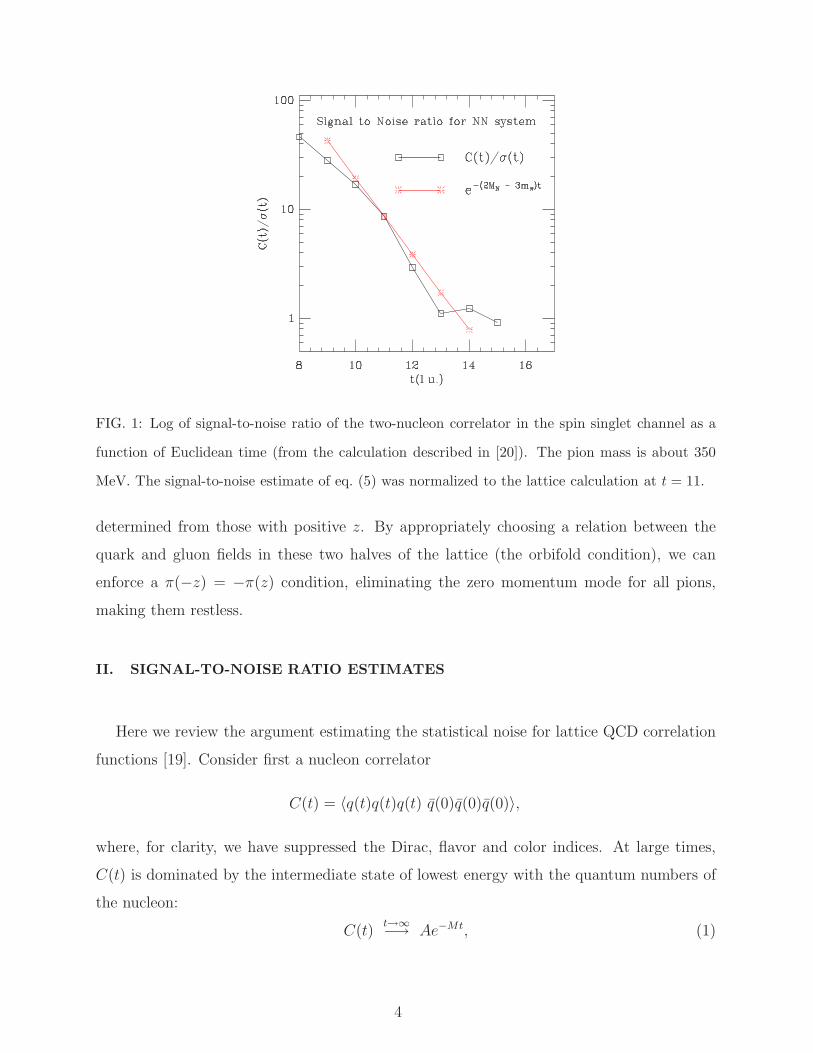
FIG. 1: Log of signal-to-noise ratio of the two-nucleon correlator in the spin singlet channel as a

function of Euclidean time (from the calculation described in [20]). The pion mass is about 350

MeV. The signal-to-noise estimate of eq. (5) was normalized to the lattice calculation at t = 11.

determined from those with positive z. By appropriately choosing a relation between the

quark and gluon fields in these two halves of the lattice (the orbifold condition), we can

enforce a π(−z) = −π(z) condition, eliminating the zero momentum mode for all pions,

making them restless.

II. SIGNAL-TO-NOISE RATIO ESTIMATES

Here we review the argument estimating the statistical noise for lattice QCD correlation

functions [19]. Consider first a nucleon correlator

C(t) = 〈q(t)q(t)q(t) q(0)q(0)q(0)〉,

where, for clarity, we have suppressed the Dirac, flavor and color indices. At large times,

C(t) is dominated by the intermediate state of lowest energy with the quantum numbers of

the nucleon:

C(t)t→∞−→ Ae−Mt, (1)

4

where M is the nucleon mass. In a Monte Carlo calculations, C(t) is estimated by an average

over N gauge configurations

C(t) ∼= C(t) =1

N

∑

A

SA(t)SA(t)SA(t)

≡ 〈S3A(t)〉, (2)

where SA(t) is the quark propagator in each one of the gauge configurations, A. The variance

in this estimate is given by

σ2C(t) =

1

N

∑

A

|SA(t)SA(t)SA(t) − C(t)|2

= 〈S3A(t)S† 3

A (t)〉 − |C(t)|2. (3)

For large times, C2(t) ∼ e−2Mt, while the large time behavior of 〈S3A(t)S† 3

A (t)〉 can be found

by noticing that

〈S3A(t)S† 3

A (t)〉 = 〈q3(t)Q3(t) q3(0)Q3(0)〉t→∞−→ Be−3mπt , (4)

where Q is a fictitious quark with identical quantum numbers and properties of the q quarks.2

The long time behavior of the correlator in eq. (4) is then dominated by the intermediate

state with the lowest energy with the quantum numbers of three qQ mesons. Since they

have the same mass as the qq mesons, this lowest energy state is given by three times the

pion mass. Thus, for sufficiently light pions, 〈S3A(t)S† 3

A (t)〉 decays at a rate smaller than

C2(t). The signal-to-noise ratio of the nucleon correlator is then given by

C(t)√

1N

σ2C(t)

t→∞−→ A√

Ne−Mt

e−3

2mπt

∼√

Ne−(M− 3

2mπ)t . (5)

We show in fig. (1) the signal-to-noise ratio in an actual lattice QCD calculation (details of

the simulation can be found in Refs. [1, 20]) as well as the estimate in eq. (5).

The estimate in eq. (5) is easily generalized for correlation functions of multi-baryons

and baryons with strange quarks. In the case of two-nucleon correlators, for example, the

2 This explains why the twisted and hybrid boundary conditions do not help the signal-to-noise problem.

The fictitious Q quarks have the same boundary conditions as the q quarks, and thus the qQ and Qq

mesons have periodic boundary conditions and are allowed a zero-momentum mode.

5

signal-to-noise ratio is proportional to√

Ne−(2M−3mπ)t. Recent lattice studies of nuclear

forces (and hyperon-nucleon interactions) were severely hindered by the fast decrease of

the signal-to-noise ratio with time [1, 3]. The correlators at short times cannot be used for

fitting purposes since it is contaminated by excited states3 while at later times the statistical

noise overwhelms the signal, leaving only a very narrow plateau from which the physics is

extracted. This is in stark contrast to lattice calculations of ππ interactions [21] and other

two-meson systems [22].

III. PARITY ORBIFOLDS

Let us now describe the basic idea of the orbifold construction in the case when only

one dimension is orbifolded. Consider a lattice whose z coordinate belongs to the interval

[0, L]. Extend it to [−L, L] and identify the points z = −L and z = L, effectively turning the

interval [−L, L] into a circle. Let all fields, φ(z), satisfy the periodic condition φ(L) = φ(−L).

Then identify the points z and −z by relating φ(z) to φ(−z), effectively transforming the

circle into a line segment (including the boundary) as shown in fig. (2). In the simplest case,

φ(z) = ±φ(−z). If the plus sign is chosen, φ(z) will be a linear combination of spatially

symmetric wavefunctions,

φ+(z) =

∞∑

n=0

A(n)+ cos

(nπz

L

)

. (6)

If, however, the minus sign is chosen then the φ(z) will be a linear combination of anti-

symmetric wavefunctions,

φ−(z) =

∞∑

n=1

A(n)− sin

(nπz

L

)

, (7)

and consequently there is no zero mode for this field. The lowest momentum allowed is

kmin = πL

with an energy of√

(π/L)2 + m2. This upward shift in the minimum allowed

energy value is the desired result. In order to eliminate the pions at rest we will require that

π(z) = −π(−z). The ways to achieve this by imposing orbifold conditions on the quark and

gluon fields and the generalization to higher dimensions will be discussed next.

3 In the single baryon sector, a significant improvement in the isolation of the ground state and excited

states at early times has been achieved with the use of multiple operators combined with quark and gluon

smearing [6]. The equivalent study for operators coupling to multi-nucleon states has not been performed

and is anticipated to be significantly more challenging and costly given the larger number of operators

and quark contractions.

6

z = 0

z

-z

z = Lz = -L

z = 0 z = L

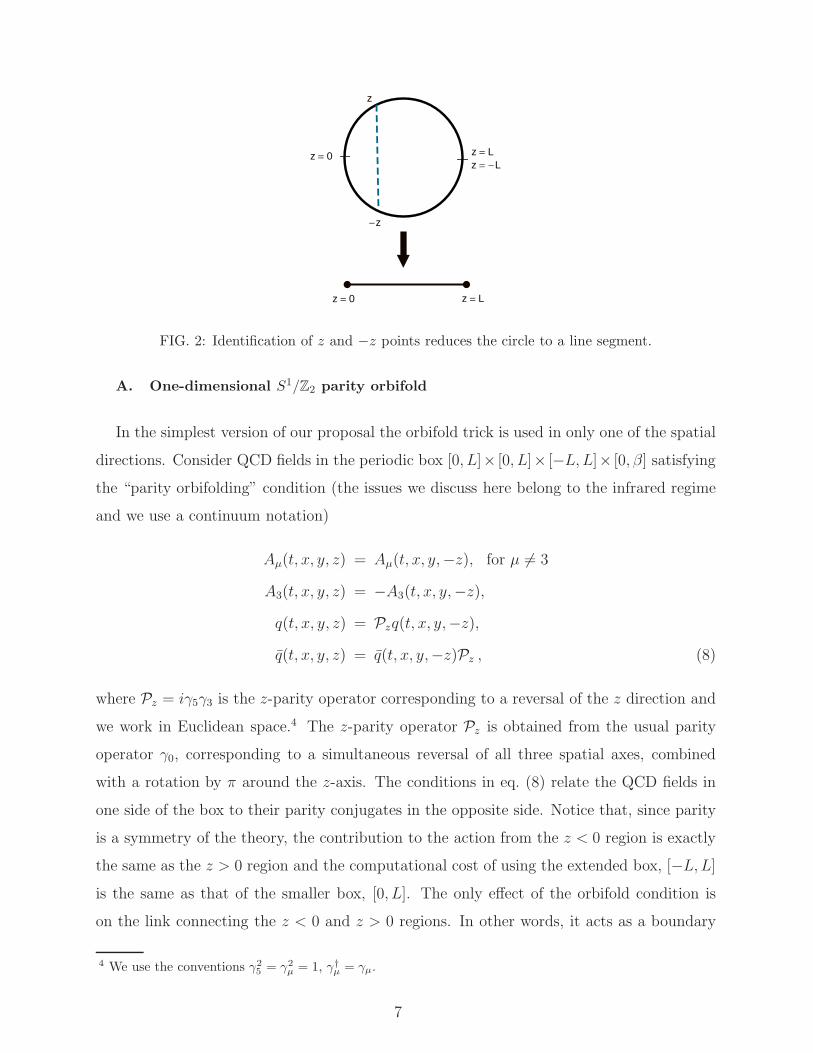
FIG. 2: Identification of z and −z points reduces the circle to a line segment.

A. One-dimensional S1/Z2 parity orbifold

In the simplest version of our proposal the orbifold trick is used in only one of the spatial

directions. Consider QCD fields in the periodic box [0, L]× [0, L]× [−L, L]× [0, β] satisfying

the “parity orbifolding” condition (the issues we discuss here belong to the infrared regime

and we use a continuum notation)

Aµ(t, x, y, z) = Aµ(t, x, y,−z), for µ 6= 3

A3(t, x, y, z) = −A3(t, x, y,−z),

q(t, x, y, z) = Pzq(t, x, y,−z),

q(t, x, y, z) = q(t, x, y,−z)Pz , (8)

where Pz = iγ5γ3 is the z-parity operator corresponding to a reversal of the z direction and

we work in Euclidean space.4 The z-parity operator Pz is obtained from the usual parity

operator γ0, corresponding to a simultaneous reversal of all three spatial axes, combined

with a rotation by π around the z-axis. The conditions in eq. (8) relate the QCD fields in

one side of the box to their parity conjugates in the opposite side. Notice that, since parity

is a symmetry of the theory, the contribution to the action from the z < 0 region is exactly

the same as the z > 0 region and the computational cost of using the extended box, [−L, L]

is the same as that of the smaller box, [0, L]. The only effect of the orbifold condition is

on the link connecting the z < 0 and z > 0 regions. In other words, it acts as a boundary

4 We use the conventions γ2

5= γ2

µ= 1, γ†

µ= γµ.

7

condition at z = 0. In fact, consider the orbifolded action in the case of Wilson quarks

S = κ [q−1(γ3 − r)q1 − q1(γ3 + r)q−1] + a4(q1q1 + q−1q−1) + · · ·

= −2κq1(γ3 + r)Pzq1 + 2a4q1q1 + · · · , (9)

where κ is the hopping parameter, the index on the quark fields denotes the position in z

(the remaining coordinates are implicit) and the dots denote the contributions from the two

sides of the bulk, z > 0 and z < 0 (which are equal to each other). We see then that the

orbifolded [−L, L] lattice is equivalent to a [0, L] lattice with some extra terms residing at

the boundary, as is the case with any boundary condition.5

Notice that we could have equally used the opposite z-parity operator, −Pz, implementing

a reversal of all three spatial axis followed by a rotation by −π about the z-axis. The

difference between rotating by π in the positive or in the negative direction amounts to a 2π

rotation which, for spin-1/2 fermions, leads to a minus sign difference between Pz and −Pz.

Physical observables, being quark bilinears, generally do not depend on this sign. As can

be seen in eq. (9), however, the boundary terms are linear in Pz and are able to distinguish

between the choice in sign of Pz. This shows that the orbifold condition breaks the z → −z

symmetry.

The parity orbifold condition on the quark and gluon fields implies orbifold conditions

for the hadronic fields. If we identify the pion field with the π ∼ qγ5τq interpolating field,

we see that it satisfies the desired

π(t, x, y, z) = −π(t, x, y,−z) (10)

orbifold condition. In fact, the same condition will follow if any other pion interpolating

field is used like, for instance, π ∼ qτqFµνFµν , since it depends only on the fact that the

pion has negative intrinsic parity. In fact, all parity odd operators will satisfy a condition

similar to eq. (10) while the parity even operators will satisfy the analogue equation without

the minus sign. In particular, the σ field σ ∼ 〈qq〉 has a zero mode and the QCD pattern of

5 Notice that, contrary to the continuum case, the boundary conditions in lattice field theory are already

contained in the action. Different lattice action terms localized at the boundary imply different boundary

conditions in the continuum and the relation between them is, in general, a complicated dynamical

question.

8

symmetry breaking is not affected by the orbifolding procedure. The nucleon fields satisfy

N(t, x, y, z) = −PzN(t, x, y,−z),

N(t, x, y, z) = −N(t, x, y,−z)Pz, (11)

as can be seen using the interpolating field N ∼ qqT τ2Cγ5q. In the non-relativistic domain,

Pz = iγ5γ3 reduces to σ3 and the allowed modes for the nucleon are

N(x, y, z) = ei nxπx2L

x+inyπy

2Ly

cos(nzπzL

)

1

0

, nx, ny, nz = 0, 1, · · ·

sin(nzπzL

)

0

1

, nx, ny = 0, 1, · · · , nz = 1, 2, · · · .

(12)

Notice that only spin up nucleons can be at rest. Consequently we can construct a spin

triplet two-nucleon state, like the deuteron, with zero momentum but a spin singlet two-

nucleon state will necessarily have a minimum momentum equal to π/L. This asymmetry

between spin up and down is a consequence of the breaking of the z → −z symmetry

discussed above.

Unfortunately, the boundary term shown in eq. (9) is not γ5-Hermitian and the fermion

determinant is not positive definite. This makes simulations with dynamical quarks sat-

isfying the parity orbifold condition impractical. However, this method is perfectly suited

to implementation in the valence sector only, i.e. only on the propagators generated in

the background of dynamical configurations. In refs. [23, 24], it was argued that up to ex-

ponentially suppressed corrections, for many channels of interest including baryon-baryon

channels, different boundary conditions can be used in the valence and sea sectors of the

theory, known as “partially twisted boundary conditions”. Therefore, gauge configurations

generated with sea quarks satisfying periodic boundary conditions can be used with valence

quarks satisfying “parity orbifold” boundary conditions. Intuitively, the possibility of using

different boundary conditions for sea and valence quarks follows from the observation that

sea quarks can “notice” their different boundary conditions only if they propagate around

the lattice. But, for observables without annihilation diagrams, the propagation of sea

quarks around the lattice is suppressed by e−mL, where m is the mass of the lightest hadron

made of sea quarks or a mixture of valence and sea quarks. In our case, this is the pion

9

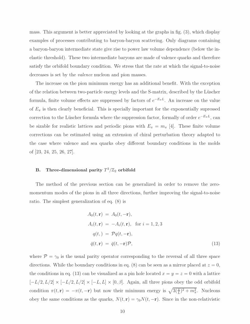
mass. This argument is better appreciated by looking at the graphs in fig. (3), which display

examples of processes contributing to baryon-baryon scattering. Only diagrams containing

a baryon-baryon intermediate state give rise to power law volume dependence (below the in-

elastic threshold). These two intermediate baryons are made of valence quarks and therefore

satisfy the orbifold boundary condition. We stress that the rate at which the signal-to-noise

decreases is set by the valence nucleon and pion masses.

The increase on the pion minimum energy has an additional benefit. With the exception

of the relation between two-particle energy levels and the S-matrix, described by the Luscher

formula, finite volume effects are suppressed by factors of e−EπL. An increase on the value

of Eπ is then clearly beneficial. This is specially important for the exponentially supressed

correction to the Luscher formula where the suppression factor, formally of order e−EπL, can

be sizable for realistic lattices and periodic pions with Eπ = mπ [4]. These finite volume

corrections can be estimated using an extension of chiral perturbation theory adapted to

the case where valence and sea quarks obey different boundary conditions in the molds

of [23, 24, 25, 26, 27].

B. Three-dimensional parity T 3/Z2 orbifold

The method of the previous section can be generalized in order to remove the zero-

momentum modes of the pions in all three directions, further improving the signal-to-noise

ratio. The simplest generalization of eq. (8) is

A0(t, r) = A0(t,−r),

Ai(t, r) = −Ai(t, r), for i = 1, 2, 3

q(t, ) = Pq(t,−r),

q(t, r) = q(t,−r)P, (13)

where P = γ0 is the usual parity operator corresponding to the reversal of all three space

directions. While the boundary conditions in eq. (8) can be seen as a mirror placed at z = 0,

the conditions in eq. (13) can be visualized as a pin hole located x = y = z = 0 with a lattice

[−L/2, L/2] × [−L/2, L/2] × [−L, L] × [0, β]. Again, all three pions obey the odd orbifold

condition π(t, r) = −π(t,−r) but now their minimum energy is√

3( πL)2 + m2

π. Nucleons

obey the same conditions as the quarks, N(t, r) = γ0N(t,−r). Since in the non-relativistic

10

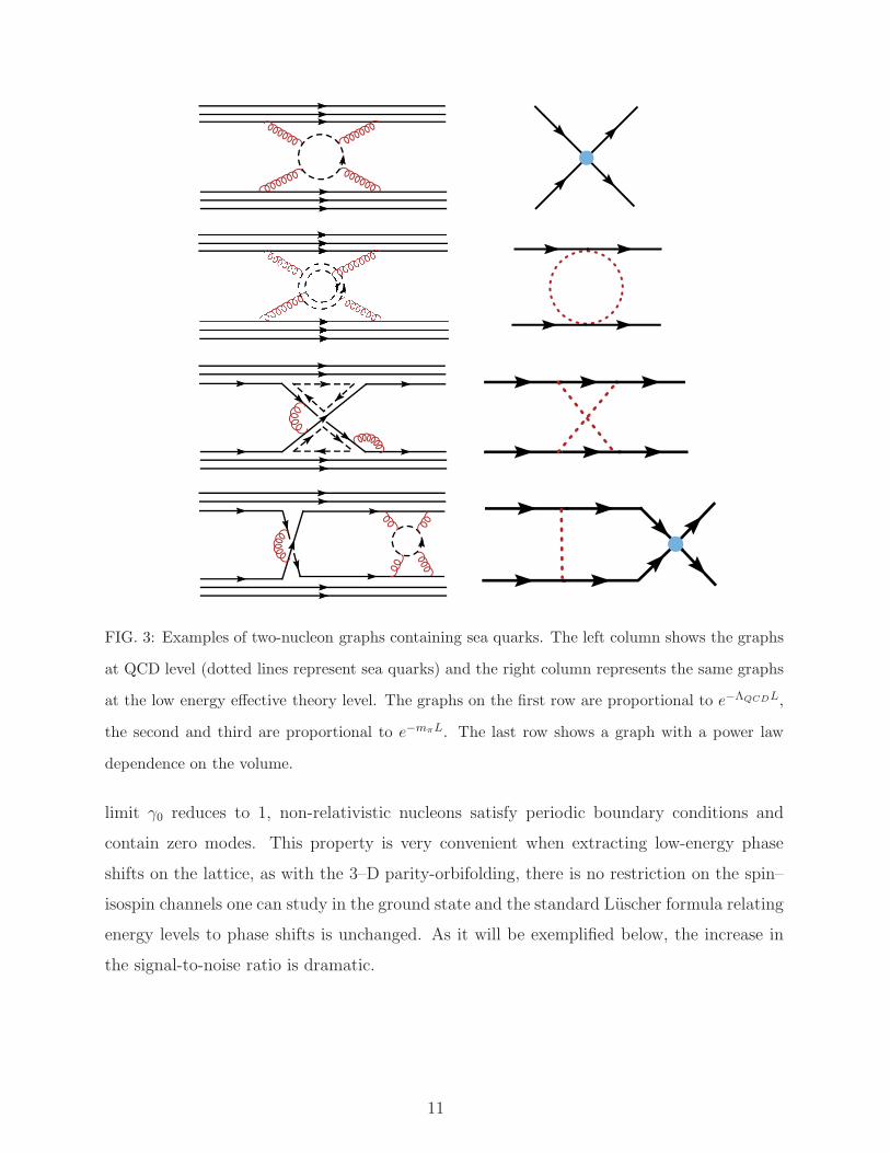
FIG. 3: Examples of two-nucleon graphs containing sea quarks. The left column shows the graphs

at QCD level (dotted lines represent sea quarks) and the right column represents the same graphs

at the low energy effective theory level. The graphs on the first row are proportional to e−ΛQCDL,

the second and third are proportional to e−mπL. The last row shows a graph with a power law

dependence on the volume.

limit γ0 reduces to 1, non-relativistic nucleons satisfy periodic boundary conditions and

contain zero modes. This property is very convenient when extracting low-energy phase

shifts on the lattice, as with the 3–D parity-orbifolding, there is no restriction on the spin–

isospin channels one can study in the ground state and the standard Luscher formula relating

energy levels to phase shifts is unchanged. As it will be exemplified below, the increase in

the signal-to-noise ratio is dramatic.

11

0.8 1 1.2 1.4 1.6 1.8 2tHfmL

0.5 1 1.5 2tHfmL

-12

-10

-8

-6

-4

-2

0

(a) (b)

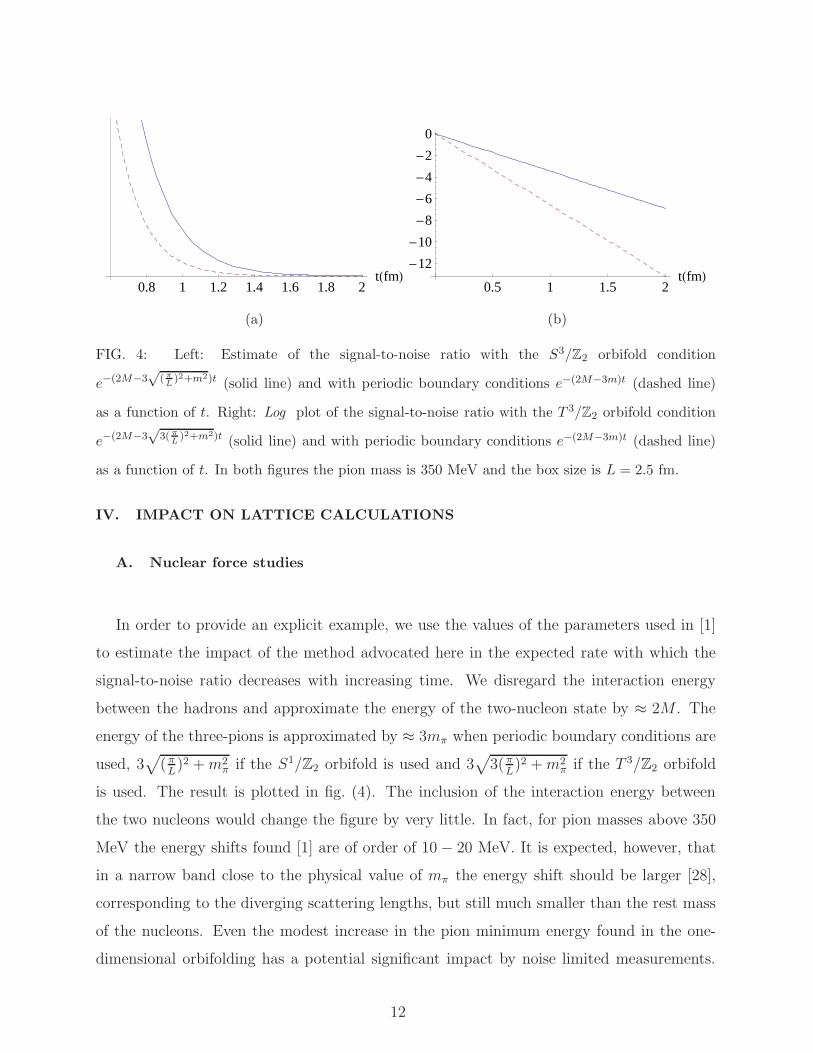
FIG. 4: Left: Estimate of the signal-to-noise ratio with the S3/Z2 orbifold condition

e−(2M−3√

( πL

)2+m2)t (solid line) and with periodic boundary conditions e−(2M−3m)t (dashed line)

as a function of t. Right: Log plot of the signal-to-noise ratio with the T 3/Z2 orbifold condition

e−(2M−3√

3( πL

)2+m2)t (solid line) and with periodic boundary conditions e−(2M−3m)t (dashed line)

as a function of t. In both figures the pion mass is 350 MeV and the box size is L = 2.5 fm.

IV. IMPACT ON LATTICE CALCULATIONS

A. Nuclear force studies

In order to provide an explicit example, we use the values of the parameters used in [1]

to estimate the impact of the method advocated here in the expected rate with which the

signal-to-noise ratio decreases with increasing time. We disregard the interaction energy

between the hadrons and approximate the energy of the two-nucleon state by ≈ 2M . The

energy of the three-pions is approximated by ≈ 3mπ when periodic boundary conditions are

used, 3√

( πL)2 + m2

π if the S1/Z2 orbifold is used and 3√

3( πL)2 + m2

π if the T 3/Z2 orbifold

is used. The result is plotted in fig. (4). The inclusion of the interaction energy between

the two nucleons would change the figure by very little. In fact, for pion masses above 350

MeV the energy shifts found [1] are of order of 10 − 20 MeV. It is expected, however, that

in a narrow band close to the physical value of mπ the energy shift should be larger [28],

corresponding to the diverging scattering lengths, but still much smaller than the rest mass

of the nucleons. Even the modest increase in the pion minimum energy found in the one-

dimensional orbifolding has a potential significant impact by noise limited measurements.

12

In the case of the three-dimensional orbifolding that potential improvement is enormous

(notice the log scale in the corresponding graph).

B. Impact on K → ππ

As pointed out in [8, 9], the extraction of the K → ππ amplitude with the Lellouch-

Luscher method [7] can benefit from eliminating pion zero modes. The method to eliminate

pions at rest discussed here can only be applied to the I = 2 channel. In the I = 0 channel,

the use of different boundary conditions in the valence and sea sectors alters the amplitude

by factors that are not exponentially suppressed. Of course, a modified chiral perturbation

theory taking into account the differences of the valence and sea sectors can still be used to

relate the results of such a lattice calculation with the real world QCD amplitude.

V. DISCUSSION

We have introduced “restless pions” boundary conditions designed to reduce the rapid

degradation of the signal-to-noise ratio which plagues studies of heavy systems with lattice

QCD. We have shown how these boundary conditions can be implemented with a parity-

orbifold construction in either one or three spatial dimensions. Unfortunately, the action

at the boundary is not γ5-Hermitian and so this particular construction is not suitable for

the sea sector. However, this method is perfectly suited for implementation of the valence

fermions. For non-scalar channels, the difference in sea and valence boundary conditions is

felt only by exponentially small terms. The numerical cost of implementing these parity-

orbifolded valence propagators is the same for propagators with (anti)-periodic boundary

conditions, as the fields in each half of the bulk are not independent, and therefore the

implementation is achieved with a special boundary condition on the non-doubled lattice.

Acknowledgments

We would like to thank T. Cohen and K. Orginos for conversations on this subject and

the NPLQCD collaboration for the use of their data in fig. (1). This research was supported

13

in part by the U.S. Dept. of Energy under grant no. DE-FG02-93Er-40762.

[1] S. R. Beane, P. F. Bedaque, K. Orginos and M. J. Savage, Phys. Rev. Lett. 97, 012001 (2006)

[arXiv:hep-lat/0602010].

[2] N. Ishii, S. Aoki and T. Hatsuda, arXiv:nucl-th/0611096.

[3] S. R. Beane, P. F. Bedaque, T. C. Luu, K. Orginos, E. Pallante, A. Parreno and M. J. Savage

[NPLQCD Collaboration], arXiv:hep-lat/0612026.

[4] I. Sato and P. F. Bedaque, arXiv:hep-lat/0702021.

[5] J. W. Chen, D. O’Connell and A. Walker-Loud, arXiv:hep-lat/07060035.

[6] S. Basak et al., Phys. Rev. D 72, 094506 (2005) [arXiv:hep-lat/0506029]; S. Basak et

al. [Lattice Hadron Physics Collaboration (LHPC)], Phys. Rev. D 72, 074501 (2005)

[arXiv:hep-lat/0508018]; S. Basak et al., PoS LAT2005, 076 (2006) [arXiv:hep-lat/0509179];

A. C. Lichtl, arXiv:hep-lat/0609019; S. Basak et al., arXiv:hep-lat/0609052; S. Basak et al.

[Lattice Hadron Physics Collaboration], PoS LAT2006, 197 (2006) [arXiv:hep-lat/0609072].

[7] L. Lellouch and M. Luscher, Commun. Math. Phys. 219, 31 (2001) [arXiv:hep-lat/0003023].

[8] C. H. Kim and N. H. Christ, Nucl. Phys. Proc. Suppl. 119, 365 (2003) [arXiv:hep-lat/0210003].

[9] C. H. Kim, Nucl. Phys. Proc. Suppl. 129, 197 (2004) [arXiv:hep-lat/0311003].

[10] P. F. Bedaque, Phys. Lett. B 593, 82 (2004) [arXiv:nucl-th/0402051].

[11] U. J. Wiese, Nucl. Phys. B 375, 45 (1992);

[12] N. Ishii, T. Doi, H. Iida, M. Oka, F. Okiharu and H. Suganuma, Phys. Rev. D 71, 034001

(2005) [arXiv:hep-lat/0408030]; N. Ishii, T. Doi, Y. Nemoto, M. Oka and H. Suganuma, Phys.

Rev. D 72, 074503 (2005) [arXiv:hep-lat/0506022].

[13] H. Iida, T. Doi, N. Ishii, H. Suganuma and K. Tsumura, Phys. Rev. D 74, 074502 (2006)

[arXiv:hep-lat/0602008].

[14] H. Suganuma, K. Tsumura, N. Ishii and F. Okiharu, arXiv:0707.3309 [hep-lat].

[15] K. R. Dienes, E. Dudas and T. Gherghetta, Nucl. Phys. B 537, 47 (1999)

[arXiv:hep-ph/9806292].

[16] D. B. Kaplan, Phys. Lett. B 288, 342 (1992) [arXiv:hep-lat/9206013].

[17] M. Luscher, arXiv:hep-th/0102028.

[18] Y. Taniguchi, JHEP 0512, 037 (2005) [arXiv:hep-lat/0412024], S. Sint, PoS LAT2005, 235

14

(2006) [arXiv:hep-lat/0511034], M. Luscher, JHEP 0605, 042 (2006) [arXiv:hep-lat/0603029].

[19] G. P. Lepage, “The Analysis Of Algorithms For Lattice Field Theory”, lectures given at

TASI’89 Summer School, Boulder, CO, 1989.

[20] S. R. Beane, K. Orginos and M. J. Savage, Nucl. Phys. B 768, 38 (2007)

[arXiv:hep-lat/0605014]; S. R. Beane, K. Orginos and M. J. Savage, arXiv:hep-lat/0604013.

[21] S. R. Sharpe et al. Nucl. Phys. B 383, 309 (1992); R. Gupta et al. Phys. Rev. D 48, 388 (1993);

Y. Kuramashi et al. Phys. Rev. Lett. 71, 2387 (1993); M. Fukugita et al. Phys. Rev. D 52,

3003 (1995); C. A. Liu et al. arXiv:hep-lat/0109010; S. Aoki et al. [JLQCD Collaboration],

Phys. Rev. D 66, 077501 (2002); S. Aoki et al. [CP-PACS Collaboration], Phys. Rev. D 67,

014502 (2003); T. Yamazaki et al. [CP-PACS Collaboration], Phys. Rev. D 70, 074513 (2004);

X. Du et al. Int. J. Mod. Phys. A 19, 5609 (2004); S. Aoki et al. [CP-PACS Collaboration],

Phys. Rev. D 71, 094504 (2005); S. R. Beane et al. [NPLQCD Collaboration], Phys. Rev. D

73, 054503 (2006); S. R. Beane et al. [NPLQCD Collaboration], arXiv:0706.3026 [hep-lat].

[22] C. Miao et al. Phys. Lett. B 595, 400 (2004);

S. R. Beane et al. [NPLQCD Collaboration], Phys. Rev. D 74, 114503 (2006);

[23] C. T. Sachrajda and G. Villadoro, Phys. Lett. B 609, 73 (2005) [arXiv:hep-lat/0411033].

[24] P. F. Bedaque and J. W. Chen, Phys. Lett. B 616, 208 (2005) [arXiv:hep-lat/0412023].

[25] B. C. Tiburzi, Phys. Lett. B 617, 40 (2005) [arXiv:hep-lat/0504002]; Phys. Lett. B 641, 342

(2006) [arXiv:hep-lat/0607019].

[26] C. W. Bernard and M. F. L. Golterman, Phys. Rev. D 49, 486 (1994) [arXiv:hep-lat/9306005];

S. R. Sharpe, Phys. Rev. D 56, 7052 (1997) [Erratum-ibid. D 62, 099901 (2000)]

[arXiv:hep-lat/9707018]; S. R. Sharpe and N. Shoresh, Phys. Rev. D 62, 094503 (2000)

[arXiv:hep-lat/0006017]; S. R. Sharpe and N. Shoresh, Phys. Rev. D 64, 114510 (2001)

[arXiv:hep-lat/0108003];

[27] J. N. Labrenz and S. R. Sharpe, Phys. Rev. D 54, 4595 (1996) [arXiv:hep-lat/9605034];

J. W. Chen and M. J. Savage, Phys. Rev. D 65, 094001 (2002) [arXiv:hep-lat/0111050];

S. R. Beane and M. J. Savage, Nucl. Phys. A 709, 319 (2002) [arXiv:hep-lat/0203003];

[28] S. R. Beane, P. F. Bedaque, A. Parreno and M. J. Savage, Phys. Lett. B 585, 106 (2004)

[arXiv:hep-lat/0312004].

15