arX

iv:h

ep-t

h/04

0711

2v3

30

Aug

200

5

Preprint typeset in JHEP style - HYPER VERSION

On Orbifold Compactification of N = 2

Supergravity in Five Dimensions

F. P. Zena, B. E. Gunaraa, Ariantoa,b and H. Zainuddinc

aTheoretical Physics Laboratory, Department of Physics,

Institute of Technology Bandung

Jl. Ganesha 10 Bandung 40132, Indonesia.

bDepartment of Physics, Udayana University

Jl. Kampus Bukit Jimbaran Denpasar 80361, Indonesia.

cTheoretical Studies Laboratory, ITMA, Universiti Putra Malaysia,

43400 UPM Serdang, Selangor, Malaysia.

E-mail: fpzen@fi.itb.ac.id, bobby@fi.itb.ac.id, ariphys@student.fi.itb.ac.id,

hisham@fsas.upm.edu.my.

Abstract: We study compactification of five dimensional ungauged N = 2 super-

gravity coupled to vector- and hypermultiplets on orbifold S1/Z2. In the model, the

vector multiplets scalar manifold is arbitrary while the hypermultiplet scalars span

a generalized self dual Einstein manifold constructed by Calderbank and Pedersen.

The bosonic and the fermionic sectors of the low energy effective N = 1 supergravity

in four dimensions are derived.

Contents

1. Introduction 1

2. Ungauged five dimensional N = 2 supergravity 2

2.1 Pure gravitational multiplet 3

2.2 Couplings of vector- and hypermultiplets 3

2.2.1 The scalar manifold 3

2.2.2 Toric Self Dual Einstein Spaces 4

3. Compactification on the orbifold S1/Z2 5

3.1 Analysis of the orbifold transformation 5

3.2 The bosonic sector 9

3.3 The fermionic sector 11

4. Conclusions and Outlook 15

A. Conventions and Notations 16

B. Five dimensional Supergravity on S1 16

C. Some detailed calculations of the fermionic sectors 18

1. Introduction

Compactification of the five dimensional N = 2 supersymmetry on singular space

S1/Z2 has achieved phenomenological interest since it provides N = 1 supersym-

metry in four dimensions. Furthermore, four dimensional N = 1 vacua for the

supersymmetric versions of the two branes Randall-Sundrum scenario of the five di-

mensional N = 2 supergravity has been obtained in [1]. In this scenario one places

two 3-branes with opposite tension at the orbifold S1/Z2 which is the boundaries

of (4+1)-dimensional Anti de Sitter spacetime. The distance between the branes is

set by the expectation value of a modulus field, called radion. Furthermore, starting

from the simplest model, namely pure supergravity theory one can derive the effec-

tive N = 1 theory as it was shown in [2].

A model consists of single hypermultiplet whose moduli space of toric self-dual

– 1 –

Einstein (TSDE) in five dimensional N = 2 supergravity has been studied to con-

struct domain wall solutions [3]. They investigated the associated supersymmetric

flows to prove the existence of domain walls which admit Randall-Sundrum flows.

However, in this model, the Kahler subspace of the TSDE is still unclear.

The purpose of this paper is to obtain a four dimensional N = 1 theory via

S1/Z2 compactification of the five dimensional N = 2 supergravity coupled to ar-

bitrary vector multiplets and a hypermultiplet which is chosen to be a generalized

self dual Einstein manifold admitting torus symmetry constructed by Calderbank

and Pedersen [4]. Our aim is to find the Kahler subspace of toric self dual Einstein

(TSDE) spaces.

Our starting point is the five dimensional N = 2 supergravity coupled to arbi-

trary vector multiplets and a hypermultiplet. First, the theory can be compactified

down to four dimensions along an S1 of radius R parametrized by x5, resulting in a

nonchiral four dimensional N = 2 theory. However, we are interested in the chiral

four dimensional N = 1 theory. Second, to obtain a chiral four dimensional N = 1

theory, we consider compactification of the x5 coordinate on the S1/Z2 orbifold. The

Z2 action is as usual x5 → −x5 and two fixed points are at x5 = 0 and x5 = πR. We

begin to mod S1 by Z2. In order the reduction to be consistent, we must first make

a certain parity assignment to the fields such that the Lagrangian is invariant under

x5 → −x5. Then, when S1 is modded out by Z2, only the even parity fields survive

on the two fixed points.

The paper is organized as follows. Section 2 briefly reviews the ungauged five

dimensional N = 2 supergravity coupled to vector- and hypermultiplets. We present

the action of the ungauged five dimensional N = 2 supergravity. Section 3 presents

a detailed derivation of the compactification of five dimensional N = 2 supergravity

coupled to vector multiplets and hypermultiplets. First, we discuss some basic analy-

sis of the S1/Z2 orbifold compactification. The starting point is the bosonic sector of

the five dimensional N = 2 supergravity theory. Second, after modding out Z2, the

odd fields are projected out and the surviving fields fit into multiplets of the chiral

four dimensional N = 1 supergravity. The boundary action arising from dimen-

sional reduction can be constructed in a straightforward way and it is obtained by

truncating four dimensional N = 1 supergravity according to the Z2 projection. We

present then the resulting of the compactification of the bosonic and the fermionic

sector. We conclude our results in section 4. Finally, in Appendices A, B and C we

summarize our notation, convention and some of the detailed calculations.

2. Ungauged five dimensional N = 2 supergravity

This section describes supergravity theory in five dimensions with N = 2 super-

symmetry in which a supergravity multiplet is coupled to matter multiplets. The

coupling to vector multiplets was given in [5, 6] and the addition of tensor multiplets

– 2 –

was considered in [7]. Furthermore, the full couplings of N = 2 supergravity theory

in five dimensions was constructed in [8].1

2.1 Pure gravitational multiplet

Five dimensional gravitational multiplet consists of the metric gµν , doublet sym-

plectic Majorana gravitinos ψiµ and a vector field Aµ (graviphoton) [10]. The greek

hatted indices are five dimensional space-time indices and run over values 0, . . . , 3, 5.

The index i of the gravitinos runs from 1 to 2.

The bosonic part of the action for the gravitational multiplet takes the form:

S = − 1

2κ25

∫

d5x√

−g[

R + FµνFµν +

1

6√

2√−g

ǫµνρσλFµνFρσAλ

]

. (2.1)

Furthermore, one can also couple the pure N = 2 gravitational multiplet to arbitrary

number of vector- and hypermultiplets. This will be discussed in the next section.

2.2 Couplings of vector- and hypermultiplets

2.2.1 The scalar manifold

First, let us describe nV vector multiplets of N = 2 supergravity2. We now have

nV +1 vector fields AIµ, nV symplectic pairs of gauginos λia, and nV real scalars φx. It

is convenient to group vectors with the graviphoton so that the index I = 0, 1, . . . , nVand a = 1, . . . , nV are corresponding flat space indices. The kinetic term of the scalars

defines the sigma model:

Lkin = −1

2gxy(φ)∂µφ

x∂µφy. (2.2)

The vector multiplet scalars φx, x = 1, . . . , nV , parametrize the target space S where

x represents curved indices. The metric gxy can be interpreted as a metric on a

Riemannian manifold S called the very special real geometry because it can be viewed

as a hypersurface by an nV polynomial of degree three

N(h) = CIJKhIhJhK = 1 , (2.3)

where hI = hI(φx). Moreover, the gauge coupling of the theory can be expressed as

aIJ(h) = −1

3

∂

∂hI∂

∂hJlnN(h)|N=1 . (2.4)

Restricting to the submanifold we can then write the metric gxy(φ) as:

gxy(φ) =∂hI

∂φx∂hJ

∂φyaIJ(h). (2.5)

1See also [9] and references therein.2We omit tensor multiplets for simplicity. For N = 2 supergravity coupled to tensor multiplets

see [7].

– 3 –

Secondly, we discuss nH hypermultiplets in which it contains 4nH real scalars qX

and 2nH symplectic Majorana fermions (hyperinos) ζA where X = 1, . . . , 4nH and

A = 1, . . . , 2nH . As in the previous case, the central object is the metric gXY of the

sigma model:

Lkin = −1

2gXY (q)∂µq

X∂µqY . (2.6)

Again, gXY is the metric on a Riemannian manifold Q on which the scalars qX

are the coordinates and thus X = 1, . . . , 4nH are the curved indices labelling the

coordinates. Local supersymmetry further implies that Q has to be a quaternionic

Kahler manifold [11].

Thus from the above discussion it shows that the scalar manifold M is a direct

product of a very special manifold S and a quaternionic manifold Q:

M = S ⊗Q, (2.7)

with φx ∈ S, qX ∈ Q.

We now write the action of N = 2 supergravity which is needed for our analysis3

S =

∫

d5x√

−g[

1

2κ25

R− 1

4aIJ F

IµνF

Jµν − 1

2gxy∂µφ

x∂µφy − 1

2gXY ∂µq

X∂µqY

− 1

2κ25

ψργρµνDµψν −

1

2λxγ

µDµλx − ζAγµDµζA

+1

6√

6√−g

ǫµνρσλCIJKFIµνF

JρσA

Kλ− i

√6

16κ5

hIFcdIψaγabcdψ

b

+iκ5

4

√

2

3

(

1

4gxyhI + Txyzh

zI

)

λxγabF Iabλy +

iκ5

8

√6hI ζAγ

abF IabζA

]

, (2.8)

where the covariant derivatives are given by

Dµλxi = ∂µλ

xi + ∂µφyΓxyzλ

zi +1

4ωµ

abγabλxi + ∂µq

XωXjiλxj, (2.9)

DµζA = ∂µζ

A + ∂µqXωXB

AζB +1

4ωµ

bcγbcζA, (2.10)

Dµψiν =

(

∂µ +1

4ωµ

bcγbc

)

ψiν − ∂µqXωX

ijψνj . (2.11)

2.2.2 Toric Self Dual Einstein Spaces

Let us now consider the hypermultiplet sector that is four dimensional (nH = 1)

which has self dual property beside Einstein spaces. Our choice is the most general

space admitting T 2 isometry which has been shown in [4]. The metric has the form

ds2 = −[

1

4ρ2− (f 2

ρ + f 2η )

f 2

]

(

dρ2 + dη2

)

3For complete action see [9].

– 4 –

−

(

(f − 2ρfρ)α− 2ρfηβ)2

+(

− 2ρfηα+ (f + 2ρfρ)β)2

f 2

(

f 2 − 4ρ2(f 2ρ + f 2

η )) , (2.12)

where α =√ρdφ and β = (dψ + ηdφ). The function f(ρ, η) satisfies the Laplace

equation in two dimensional hyperbolic space spanned by (ρ, η)

ρ2(fρρ + fηη) =3

4f, (2.13)

with fρρ = ∂2f∂ρ2

and fηη = ∂2f∂η2

. One takes ρ > 0 and η ∈ R while (φ, ψ) are

periodic coordinates. Furthermore, it has positive scalar curvature if f satisfies

f 2 > 4ρ2(f 2ρ + f 2

η ) and negative if f 2 < 4ρ2(f 2ρ + f 2

η ).

3. Compactification on the orbifold S1/Z2

3.1 Analysis of the orbifold transformation

Now we turn our attention to consider the five dimensional supergravity on the

orbifold S1/Z24. As we shall see that the five dimensional N = 2 supergravity is

reduced to four dimensional N = 1 supergravity.

There are two ways to employ the compactification on orbifold. In the so-called

downstair approach, we consider the five dimensional supergravity with x5 ∈ S1/Z2 =

[0, πR], so x5 ∼ x5 + 2πR and x5 ∼ −x5. Then, the five dimensional space-time is

M5down = M4 × (S1/Z2) = M4 × [0, πR]. Locally, we still have ordinary the five

dimensional supergravity, but on boundary special thing can occur. The boundary

consist of two four dimensional space-time, one at x5 = 0 called M4 and one at

x5 = πR called M ′4.

In the so called upstair approach, we consider the five dimensional supergravity

with x5 on S1 so that x5 ∼ x5 + 2πR and the five dimensional space-time is M5up =

M4 × S1. Then, we define the orbifold transformation O by

O : x5→−x5, xµ→xµ. (3.1)

The fixed points of O are the points with x5 = 0 or x5 = πR, so the fixed points

consist of two four dimensional space-time M4 and M ′4 which are the boundary

of M5up. To get the same picture as in the downstair approach, we demand that

the physics should be invariant under the orbifold transformation O. We must in

particular have the distance ds2 invariant,

ds2 = gµνdxµdxν

= gµνdxµdxν + 2gµ5dx

µdx5 + g55dx5dx5

→ gµνdxµdxν + 2gµ5dx

µ(−dx5) + g55(−dx5)(−dx5). (3.2)4We discuss S1 compactification in Appendix B.

– 5 –

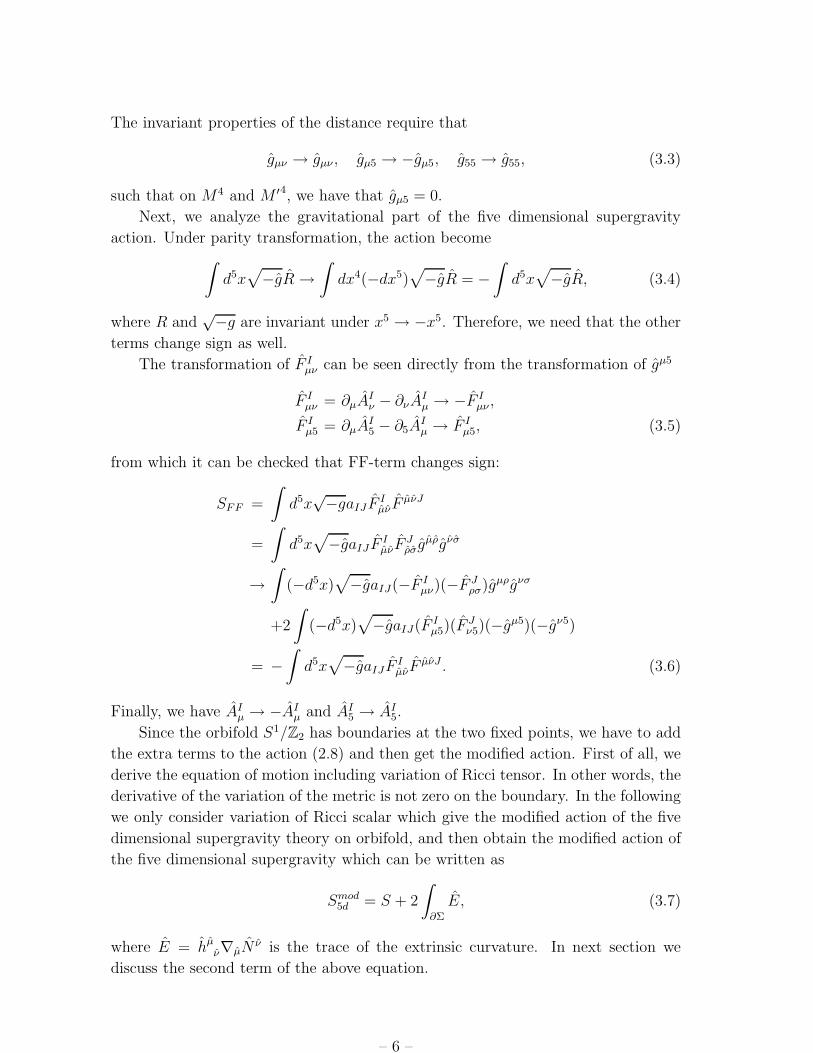
The invariant properties of the distance require that

gµν → gµν , gµ5 → −gµ5, g55 → g55, (3.3)

such that on M4 and M ′4, we have that gµ5 = 0.

Next, we analyze the gravitational part of the five dimensional supergravity

action. Under parity transformation, the action become∫

d5x√

−gR →∫

dx4(−dx5)√

−gR = −∫

d5x√

−gR, (3.4)

where R and√−g are invariant under x5 → −x5. Therefore, we need that the other

terms change sign as well.

The transformation of F Iµν can be seen directly from the transformation of gµ5

F Iµν = ∂µA

Iν − ∂νA

Iµ → −F I

µν ,

F Iµ5 = ∂µA

I5 − ∂5A

Iµ → F I

µ5, (3.5)

from which it can be checked that FF-term changes sign:

SFF =

∫

d5x√−gaIJ F I

µνFµνJ

=

∫

d5x√

−gaIJ F IµνF

Jρσg

µρgνσ

→∫

(−d5x)√

−gaIJ(−F Iµν)(−F J

ρσ)gµρgνσ

+2

∫

(−d5x)√

−gaIJ(F Iµ5)(F

Jν5)(−gµ5)(−gν5)

= −∫

d5x√

−gaIJF IµνF

µνJ . (3.6)

Finally, we have AIµ → −AIµ and AI5 → AI5.

Since the orbifold S1/Z2 has boundaries at the two fixed points, we have to add

the extra terms to the action (2.8) and then get the modified action. First of all, we

derive the equation of motion including variation of Ricci tensor. In other words, the

derivative of the variation of the metric is not zero on the boundary. In the following

we only consider variation of Ricci scalar which give the modified action of the five

dimensional supergravity theory on orbifold, and then obtain the modified action of

the five dimensional supergravity which can be written as

Smod5d = S + 2

∫

∂Σ

E, (3.7)

where E = hµν∇µNν is the trace of the extrinsic curvature. In next section we

discuss the second term of the above equation.

– 6 –

The variation of the five dimensional Ricci scalar is given by

δS =

∫

d5x

[

δ√

−gR +√

−gδgµνRµν +√

−ggµνδRµν

]

=

∫

d5x√

−g[

g1

2gρσR − gµρgσνRµν

]

δgρσ

+

∫

d5x√

−g∇ρ

[

−∇ρ(gµνδgµν) + ∇µδgρµ

]

, (3.8)

where we have used

δRµν =1

2gρσ

(

−∇µ∇ν(δgρσ) + ∇ρ∇ν(δgσµ) + ∇ρ∇µ(δgσν) −∇ρ∇σ(δgµν))

, (3.9)

and the metric postulate ∇ρgµν = 0. After plugging (3.9) into (3.8), finally we get

δS =

∫

d5x√

−g[

1

2gρσR− Rρσ

]

δgρσ +

∫

d5x√

−g∇µTµ, (3.10)

where

Tµ = gνρ(∇ρδgµν −∇µδgνρ). (3.11)

Using Gauss theorem, we can rewrite the last term of (3.10):

∫

Σ

d5x∂µ(√

−gTµ) =

∫

∂Σ

d4x√

−gN µTµ, (3.12)

where N µ is the normal to the surface. This term is zero because the derivative of

the variation of the metric is zero on the boundary. This term modifies the action of

the five dimensional supergravity theory on orbifold .

Next, after assuming δgµν is a constant on the surface ∂Σ, then the equation

(3.12) can be written down as:

∫

Σ

d5x∂µ(√

−gTµ) = −∫

∂Σ

d4x√

−gN µhν ρ∇µ(δgνρ), (3.13)

where we have used hνρ∇ρδgµν = 0. The boundaries can be considered as a four

dimensional surface embedded in the five dimensional space-time.

We now define a quantity E, whose variation equals to the equation (3.13). We

have

Eµν = h ρµ ∇ρNν , hµν = gµν − NµNν , (3.14)

where

Nµ = ±δ5

µ

√

g55. (3.15)

From the above equation we see that induced metric on the surface ∂Σ has

h55 = 0. (3.16)

– 7 –

The trace of extrinsic curvature E is calculated according to

E = gµνEµν = gµνh ρµ ∇ρNν

= hνρ(∂ρNν − ΓσρνNσ) = h5ρ(∂ρN5 − Γ5ρνN5)

= h5ρ∂ρN5 −1

2g5λhνρ[∂ρgλν − ∂ν gλρ + ∂λgνρ]N5, (3.17)

where we have used definition of the Christoffel symbol.

Now we use the fact that both gµν and hµν are block diagonal

E = h55∂5N5 −1

2g55h5ρ∂ρg55

−1

2g55hν5∂ν g55 +

1

2g55hν

ˆrho∂5gνρN5

=1

2g55hνρ∂5gνρN5, (3.18)

where we have used the fact that hν5∂ν g55 = 0 since this is a derivative along the

surface and that the variation is zero on the surface. The second term of (3.7) comes

from variation of the extrinsic curvature (3.17), we get

δE =1

2N µhνρ(∇µδgνρ), (3.19)

which is identical to (3.13) apart from the factor two. Here we are working in the

massless sector of the theory, where ∂5gµν = 0 so the second term of (3.7) does not

contribute to our action. However if we are working in the massive sector, this term

can not be ignored. In the following section we only consider the massless sector to

obtain the low-energy effective action of the four dimensional N = 1 supersymmetry

theory.

From the bosonic sector analysis, the five dimensional fields can be even (Φ(x5) =

Φ(−x5)) or odd (Φ(x5) = −Φ(−x5)) under orbifold transformation. Note that the

odd fields must either vanish or be discontinuous at the fixed points, hence they

are not dynamical fields on the submanifolds. Identifying periodicity of the scalar

fields in (2.12), Φ → Φ + Φ0 with Φ ≡ (ρ, η, ψ, φ) and under orbifold transformation

Φ → −Φ, we define the fields (ρ, η) are even and (ψ, φ) are odd.5

The action of Z2 on the fermion fields and on the spinor parameter ǫ of the

supersymmetry transformations is defined as [12, 13]:

ψiµ(x5) = P(ψ)γ5M(q)ijψ

jµ(−x5) , (3.20)

λi(x5) = P(λ)γ5M(q)ijλj(−x5) , (3.21)

ǫi(x5) = P(ǫ)γ5M(q)ijεj(−x5), (3.22)

5The odd parity of (ρ, η) is not satisfied in the function F (ρ, η), for example, for F (ρ, η) =√ρ2+(η−y)2

√ρ

. See [4].

– 8 –

where

M ij = m1(q)(σ1)

ij +m2(q)(σ2)

ij +m3(q)(σ3)

ij , (3.23)

with m1, m2, m3 ∈ real functions of q and P(Ψ) = ±, Ψ ≡ (λ, ψ, ε). Decomposing

the five dimensional spinor Ψ, and its conjugate Ψ, into four-dimensional spinor, and

following the convention in [2] it is given by

Ψµ =

ψ1µL

ψ2µR

, (3.24)

and

γ5 =

−i 0

0 i

, γa =

0 σa

σa 0

. (3.25)

To complete the results of this section, we must first take certain parity assign-

ments to the fields such that the action stays invariant under x5 → −x5. Then, when

we mod out Z2, only fields of even parity survive on the two orbifold fixed points.

The even parity fields are given by

gµν , g55, AI5, ρ, η, ψ+

µ , ψ−5 , ζ1, λ1

x, ǫ+, (3.26)

and those of odd parity are given by

gµ5, g5µ, AIµ, φ, ψ, ψ−

µ , ψ+

5 , ζ2, λ2

x, ǫ−, (3.27)

where we define ψ±µ = 1√

2(ψ1

µ ± ψ2µ).

3.2 The bosonic sector

In this subsection we derive the low energy effective N = 1 action via compactifi-

cation of the bosonic part of the action of the ungauged N = 2 supergravity in five

dimensions (2.8) on the orbifold S1/Z2 using the analysis above.

Under the Z2 symmetry, the bosonic fields (gµν , g55, AI5, ρ, η) have to be even,

while (gµ5, AIµ, φ, ψ) are odd with respect to the orbifold transformation. The analy-

sis of the orbifold transformation above are similar to S1 compactification,6 however

all odd fields are ruled out. Using the ansatz,

ds2 = A(x)gµνdxµdxν +B(x)dz2, (3.28)

we find

SS1/Z2=

∫

d4√−g

[

1

2κ24

(

AB1/2R +3

2A−1B1/2∂µA∂

µA +3

2B1/2∂µA∂

µB)

−1

2

(

κ25

κ24

)

AB−1/2aIJ∂µAI5∂

µAI5 −1

2

(

κ25

κ24

)

AB1/2gxy∂µφx∂µφy

+1

2

(

κ25

κ24

)

AB1/2

(

1

4ρ2− f 2

ρ + f 2η

f 2

)

(

∂µρ∂µρ+ ∂µη∂

µη)

]

. (3.29)

6See Appendix B.

– 9 –

To put the equation (3.29) back into the canonical form, we perform a Weyl rescaling

of the metric which is given by:

gµν → gµν = A−1B−1/2gµν , gµν → gµν = AB1/2gµν . (3.30)

So under this rescaling the equation (3.29) becomes:

SS1/Z2=

∫

d4√−g

[

1

2κ24

(

R− 3

8∂µlnB∂

µlnB)

−1

2

(

κ25

κ24

)

B−1aIJ∂µAI5∂

µAI5 −1

2

(

κ25

κ24

)

gxy∂µφx∂µφy

+1

2

(

κ25

κ24

)(

1

4ρ2− f 2

ρ + f 2η

f 2

)

(

∂µρ∂µρ+ ∂µη∂

µη)

]

. (3.31)

The four dimensional gravitational constant (1/κ24) can be expressed in terms of its

five dimensional counterpart as:

κ2

4 =κ2

5

2πR. (3.32)

The equation (3.31) can be rewritten in the form:

SS1/Z2=

1

2κ24

∫

d4√−g

[

R− 1

κ25

aIJ∂µhI∂µhJ − 2

3aIJ∂µA

I5∂

µAI5

+κ2

5

(

1

4ρ2− f 2

ρ + f 2η

f 2

)

(

∂µρ∂µρ+ ∂µη∂

µη)

]

, (3.33)

where aIJ =3κ2

5

2B−1aIJ , h

I = B1/2hI and we have used the identities

hIx = −√

3

2κ25

hI,x, hIhxI = 0, gxy = aIJhIxh

Jy , aIJ = −2CIJK + 3hIhJ . (3.34)

In (3.33), nV +1 vector multiplet scalars φx appear through nV +1 scalars hI subject

to the constraint,

CIJK(h)hI hJ hK = B−3/2. (3.35)

Now we consider the low-energy effective action of N = 1 supergravity in four

dimensions. Therefore, we must show that the scalars in (3.33) parametrize a complex

manifold of the Kahler type. For that purpose, we define two new complex quantities,

T and S:

T I =1

κ5

hI + i

√

3

2AI5, (3.36)

S =1

κ5

(

ρ+ iη)

. (3.37)

– 10 –

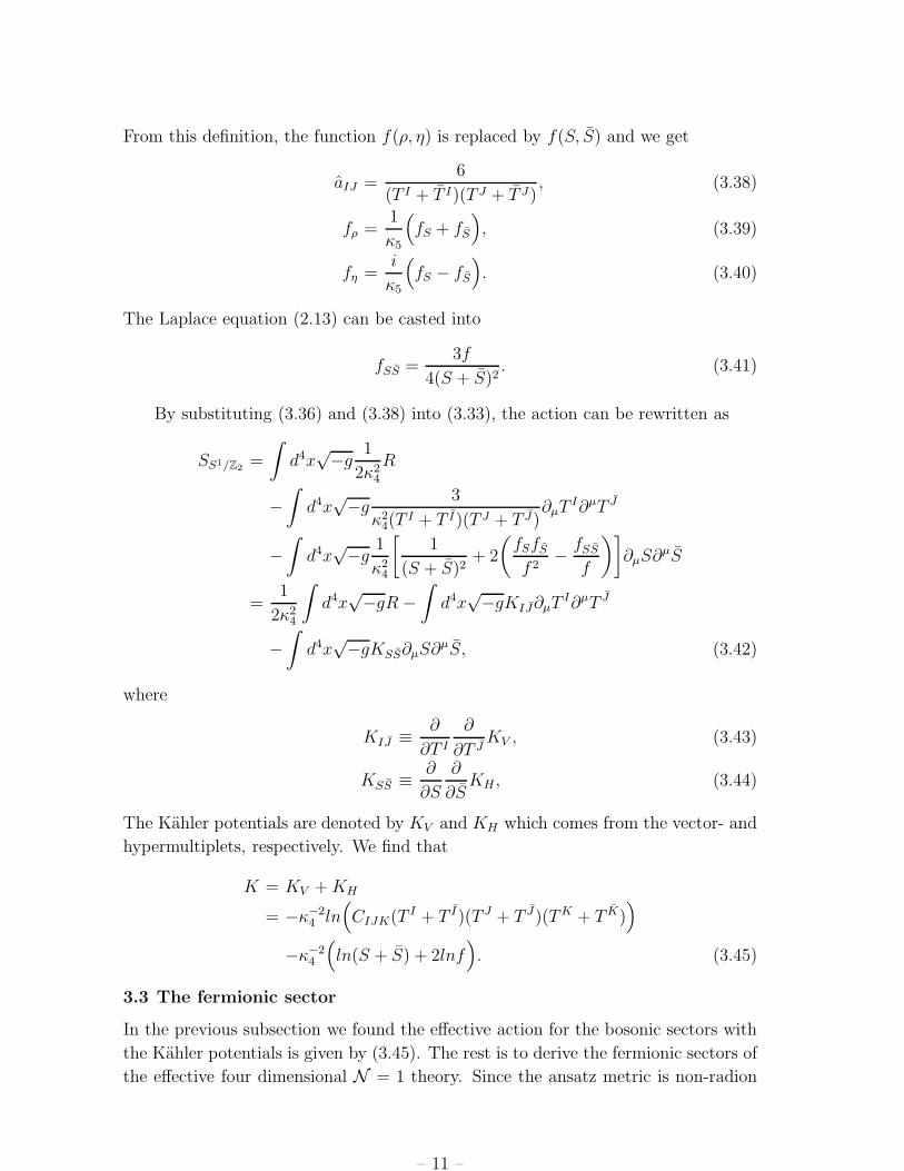
From this definition, the function f(ρ, η) is replaced by f(S, S) and we get

aIJ =6

(T I + T I)(T J + T J), (3.38)

fρ =1

κ5

(

fS + fS

)

, (3.39)

fη =i

κ5

(

fS − fS

)

. (3.40)

The Laplace equation (2.13) can be casted into

fSS =3f

4(S + S)2. (3.41)

By substituting (3.36) and (3.38) into (3.33), the action can be rewritten as

SS1/Z2=

∫

d4x√−g 1

2κ24

R

−∫

d4x√−g 3

κ24(T

I + T I)(T J + T J)∂µT

I∂µT J

−∫

d4x√−g 1

κ24

[

1

(S + S)2+ 2

(

fSfSf 2

− fSSf

)]

∂µS∂µS

=1

2κ24

∫

d4x√−gR−

∫

d4x√−gKIJ∂µT

I∂µT J

−∫

d4x√−gKSS∂µS∂

µS, (3.42)

where

KIJ ≡ ∂

∂T I∂

∂T JKV , (3.43)

KSS ≡ ∂

∂S

∂

∂SKH , (3.44)

The Kahler potentials are denoted by KV and KH which comes from the vector- and

hypermultiplets, respectively. We find that

K = KV +KH

= −κ−2

4 ln(

CIJK(T I + T I)(T J + T J)(TK + T K))

−κ−24

(

ln(S + S) + 2lnf)

. (3.45)

3.3 The fermionic sector

In the previous subsection we found the effective action for the bosonic sectors with

the Kahler potentials is given by (3.45). The rest is to derive the fermionic sectors of

the effective four dimensional N = 1 theory. Since the ansatz metric is non-radion

– 11 –

background, the fermionic fields do not depend on x5 and then the integral over the

compact dimensions in the action yields just the volume which can be absorbed into

the definition of the four dimensional gravitational constant. In other words, it is

equivalent to integrate out the massive Kaluza-Klein modes and one keeps only zero

modes in the effective description.

Our starting point is the fermionic parts of the action (2.8). The kinetic term of

the ψψ-component is given by

Sψψ =

∫

d5x√

−g[

− 1

2κ25

ψργρµνDµψν −

i√

6

16κ5

hIFIρσψµγ

µνρσψν

]

. (3.46)

It is convenient to combine two symplectic Majorana spinors into one even(odd)

Majorana spinor in four dimensions, with the following convention

ψµ =

ψ1µL

ψ2

µR

, ψµ =

(

ψ2

µL, ψ1

µR

)

. (3.47)

Using these definitions, we can rewrite (3.46) in terms of even and odd combinations,

Sψψ =

∫

d5x√

−g[

− 1

2κ25

ψ2ργ

ρµνDµψ1ν −

i√

6

16κ5

hIFIρσψ

2µγ

µνρσψ1ν

]

+ h.c., (3.48)

or

Sψψ =

∫

d5x√

−g[

− 1

2κ25

.1

2.(

ψ+

ρ γρµνDµψ

+

ν − ψ−ρ γ

ρµνDµψ−ν

)

− i√

6

16κ5

hIFIρσ

1

2

(

ψ+

µ γµνρσψ+

ν − ψ−µ γ

µνρσψ−ν

)

]

+ h.c., (3.49)

where we have used

ψ1

µ =1√2

(

ψ+

µ + ψ−µ

)

ψ2

µ =1√2

(

ψ+

µ − ψ−µ

)

. (3.50)

The two fixed points require that certain Z2-odd fields have a step-function, namely

sgn(z = x5). The step function sgn(z = x5) takes values −1 for x5 ∈ [−πR, 0] and

+1 for x5 ∈ [0, πR].

In order for the reduction to be consistent, we must make an ansatz for the

gravitino as follows

ψ+

µ =1√2C(x)ψµ, ψ−

µ =1√2sgn(z)C(x)ψµ. (3.51)

where C(x) is an arbitrary function. After subtracting to each component and plug-

ging the ansatz into (3.49) we get7

Sψψ =

∫

d5x√

−g[

− 1

2κ25

1

2

(

ψ+

ρ γρµνDµψ

+

ν + ψ+

ρ γρ5νD5ψ

−ν

)

− i√

6

16κ5

hIFIρσ

1

2ψ+

µ γµνρσψ+

ν

+1

2κ25

ψ+

ρ γρνψ+

ν (δ(z) − δ(z − πR))

]

+ h.c.. (3.52)

7The detailed calculation is presented in Appendix C.

– 12 –

We note that the third term of the action (3.52) is the boundary term. This result has

to be consistent with the upstair approach used in [14] where one regards space-time

as the smooth manifold M4 × S1 subject to Z2 symmetry. Then, in the framework

of the five dimensional supergravity we can write the total action by

S = Sbulk + Sboundary, (3.53)

where Sbulk is given by (2.8) and Sboundary or Sbrane in the context of braneworld is

given by

Sbrane =1

2κ25

∫

d5x√−gψ+

µ γµνψ+

ν [δ(z) − δ(z − πR)] + h.c. (3.54)

The bulk part of the action (3.52) can be rewritten as follows

Sψψ =1

2κ25

∫

d5x√

−g C2

4ψργ

ρµνDµψν + h.c., (3.55)

where

Dµψν = ∂µψν +1

2ωµ

abγabψν + ∂µlnCψν −1

4∂µlnBψν

−κ24

12(KI∂µT

I −KI∂µTI)ψν +

iκ24

2(KS∂µS −KS∂µS)ψν . (3.56)

After integrating (3.55) with respect to x5 ∈ [−πR, πR], we finally get

Sψψ = − 1

2κ24

∫

d4x√−gψργρµνDµψν . (3.57)

In the above expressions we have set C = B1/4 so that the covariant derivative in

four dimensions becomes

Dµψν = ∂µψν +1

2ωµ

abγabψν −κ2

4

12(KI∂µT

I −KI∂µTI)ψν

+iκ2

4

2(KS∂µS −KS∂µS)ψν , (3.58)

and then used the spin connections in the metric background,

ωµab = ωµ

ab − 1

4(eaµe

νb − ebµeνa)∂ν lnB, (3.59)

ω5a5 = −1

2B1/2eµa∂µlnB, (3.60)

and Sp(1)-connections,

ω1 = −fηfdρ+

( 1

2ρ+fρf

)

dη. (3.61)

– 13 –

The hyperino kinetic terms of the fermionic sector of the action (2.8) is given by

Sζζ =

∫

d5x√

−g[

− ζAγµDµζA +iκ5

8

√6hI ζAγ

abF IabζA

]

, A = 1, 2. (3.62)

We assume that the fields are independent of the fifth coordinate so that derivative

with respect to fifth coordinate vanishes. The ansatz for the hyperino (even fields),

ζA → ζ1 =1√2κ5

B1/4ζ, (3.63)

and we obtain

Sζζ = − 1

2κ24

∫

d4x√−gζγµDµζ. (3.64)

The covariant derivative for the hyperino in four dimensions is given by

Dµζ = ∂µζ +1

2ωµ

abγabζ −iκ2

4

2(KS∂µS−KS∂µS)ζ +

κ24

6(KI∂µT

I −KI∂µTI)ζ. (3.65)

Next we look at the gaugino kinetic terms

Sλλ =

∫

d5x√

−g[

− 1

2λxγ

µDµλx +

iκ5

4

√

2

3

(

1

4gxyhI +Txyzh

zI

)

λxγabF Iabλy

]

. (3.66)

For gaugino, the procedure is similar to the hyperino terms and we then obtain

Sλλ = − 1

2κ24

∫

d4x√−gλxγµDµλx, (3.67)

where

Dµλx = ∂µλx +1

2ωµ

abγabλx + ∂µφyΓzyxλz −

iκ24

2(KS∂µS −KS∂µS)λx

+κ2

4

12(KI∂µT

I −KI∂µTI)λx. (3.68)

Finally, by combining the results of the bosonic and the fermionic sectors we get the

low-energy effective action of N = 1 in four dimensions:

SN=1

d=4 =1

2κ24

∫

d4x√−g

[

R + ψργρµνDµψν − ζγµDµζ − λxγµDµλx

−2κ2

4KII∂µTI∂µT I − 2κ2

4KSS∂µS∂µS

]

, (3.69)

where the covariant derivative of the spinors are given by (3.58), (3.65) and (3.68).

– 14 –

4. Conclusions and Outlook

In this paper we have studied S1/Z2 compactification of the ungauged N = 1 super-

gravity in five dimensions coupled to arbitrary vector multiplets and a hypermultiplet

where the scalar fields span toric self dual Eintein spaces. The resulting theory is

four dimensional N = 1 supergravity. In the bosonic sector we found that Kahler

potential from the vector multiplets contribution has the form

KV = −κ−2

4 ln(

CIJK(T I + T I)(T J + T J)(TK + T K))

, (4.1)

and from hypermultiplets contribution are

KH = −κ−24

(

ln(S + S) + 2lnf)

. (4.2)

Furthermore, we have derived the fermionic sectors of the four dimensional N = 1

theory. In general, our results confirm those in reference [2], where the effective the-

ory was obtained by compactification from five dimensional supergravity down to

four dimensions in the context of Randall-Sundrum scenario.

It is also interesting to extend our scenario to the general case where the N = 2

scalar potential reduced to the N = 1 scalar potential in terms of holomorphic su-

perpotential. Another problem is to cancel anomaly of the orbifold model and find

the gauge group on two orbifold fixed points such that the gauge and the scalar fields

residing on the boundaries can be supersymmetrized. This can be done by modifying

the boundary action but also one has to modify the supersymmetry transformation

laws in both boundary and bulk fields. This problem will be addressed elsewhere.

Note Added: During preparation of this manuscript we became aware of the

independent work [15] which has some overlaps with our results.

– 15 –

A. Conventions and Notations

The purpose of this appendix is to collect our conventions in this paper. The space-

time metric is taken to have the signature (−,+,+,+,+) while the Ricci scalar is

defined to be R = gµν[

1

2∂ρΓ

ρµν − ∂νΓ

ρµρ + ΓσµνΓ

ρσρ

]

+ 1

2∂ρ

[

gµνΓρµν

]

. The Christoffel

symbol is given by Γµνρ = 1

2gµσ(∂νgρσ + ∂ρgνσ − ∂σgνρ) where gµν is the spacetime

metric.

Indices

µ, ν = 0, ..., 3, 5 label curved five dimensional spacetime indices

a, b = 0, ..., 3, 5 label flat five dimensional spacetime indices

µ, ν = 0, ..., 3 label curved four dimensional spacetime indices

a, b = 0, ..., 3 label flat four dimensional spacetime indices

i, j = 1, 2 label the fundamental representation of

the R-symmetry group SU(2) ⊗ U(1)

x, y, z = 1, .., nV label the real scalars of the N = 2 vector multiplet

I, J,K = 0, 1, .., nV label the vector multiplets

X, Y, Z = 1, ..., 4nH label the real scalars of the N = 2 hypermultiplet

A,B = 1, ..., 2nH label the fundamental representation of Sp(2nH)

B. Five dimensional Supergravity on S1

In this section, we derive the dimensional reduction of the bosonic part of the five

dimensional supergravity action on S1.8 The class of four dimensional theories ob-

tained in this way are only a subclass of the general four dimensional N = 2 theories

[17]. In general, we can choose the metric to be

ds25 = A(x)gµνdx

µdxν +B(x)dz2

= gµνdxµdxν (B.1)

where A and B are arbitrary functions. We have

gµν = A(x)gµν gzz = B(x). (B.2)

8This has also been discussed in the appendix of [16].

– 16 –

The gravity term in the supergravity Lagrangian reduced to

√

−gR ∼ √−g[

AB1/2R +3

2A−1B1/2∂µA∂

µA+3

2B−1/2∂µA∂

µB]

, (B.3)

where ∼ means equal up to a total derivative. The FF-term we are going to reduce

is

LFF = −1

4

√

−gaIJ F IµνF

µνJ .

In order to get the massless sector we divide F Iµν into (F I

µν , FIµ5). Then, we take

Fourier expansion of this term and keep only the lowest order terms which should be

independent of x5. We then have that

−1

4

√

−gaIJ F IµνF

µνJ = −1

4

√−gB1/2aIJFIµνF

µνJ

−1

2

√−gAB−1/2aIJ∂µAI5∂

µAJ5 , (B.4)

where AI5 are the fifth component of the vector fields. The vector multiplet scalars

sector reduce to

Lφ = −1

2

√

−ggxy∂µφx∂µφy

= −1

2

√−gAB1/2gxy∂µφx∂µφy. (B.5)

The hypermultiplet sector reduce to

Lq = −1

2

√

−ggXY ∂µqX∂µqY

= −1

2

√−gAB1/2gXY ∂µqX∂µqY . (B.6)

Moreover The Chern-Simon term can be simplified

LFFA =1

6√

6ǫµνρσλCIJKF

IµνF

JρσA

Kλ

=1

2√

6ǫµνρσCIJKF

IµνF

JρσA

K5

=1

2√

6ǫµνρσCIJKF

IµνF

JρσA

K5 . (B.7)

Collecting the above results, the bosonic part of the reduced supergravity Lagrangian

(2.8) is

1√−gLS1

4d = −1

2AB1/2R− 3

4∂µlnA∂

µlnA− 3

4∂µlnA∂

µlnB

−1

2AB1/2gxy∂µφ

x∂µφy − 1

4B1/2aIJF

IµνF

µνJ

−1

2AB−1/2aIJ∂µA

I5∂

µAJ5 − 1√6CIJKF

IµνF

µνJAK5 . (B.8)

– 17 –

Here, we only consider the arbitrary function A = A(x) and B = B(x). To put

the equation (B.8) back into the canonical form, we perform a Weyl rescaling of the

metric which is given by:

gµν → A−1B−1/2gµν . (B.9)

So under this rescaling the lagrangian becomes:

1√−gLS1

4d =1

2R− aIJ(hI)∂µh

I∂µhJ − 2

3aIJ(hI)∂µA

I5∂

µAJ5

−1

4B1/2aIJF

IµνF

µνJ +1√6CIJKF

IµνF

µνJAK5 , (B.10)

where aIJ = 3

4B−1aIJ and hI = B1/2hI . The Chern-Simons term vanishes identically

for the non abelian case.

C. Some detailed calculations of the fermionic sectors

The five dimensional spinor Ψ and its conjugate Ψ can be written into four dimen-

sional form which are Ψ ≡ (ψ1L, ψ

2R)T and Ψ ≡ (ψ2L, ψ1

R). Plugging this definition

into (3.49) we get

Sψψ =

∫

d5x√

−g[

− 1

2κ25

ψ2

ργρµνDµψ

1

ν −1

2κ25

ψ1

ργρµνDµψ

2

ν

− i√

6

16κ5

hIFIρσψ

2

µγµνρσψ1

ν −i√

6

16κ5

hIFIρσψ

1

µγµνρσψ

2

ν

]

. (C.1)

By using ψ1µ = 1√

2(ψ+

µ + ψ−µ ) and ψ2

µ = 1√2(ψ+

µ − ψ−µ ), (C.1) can be rewritten as

Sψψ =

∫

d5x√

−g[

− 1

2κ25

1

2

(

ψ+

ρ γρµνDµψ

+

ν − ψ−ρ γ

ρµνDµψ−ν

)

− i√

6

16κ5

hIFIρσ

1

2

(

ψ+

µ γµνρσψ+

ν − ψ−µ γ

µνρσψ−ν

)]

+ h.c.. (C.2)

Now we split the space-time coordinates into: xµ = (xµ, x5),

Sψψ =

∫

d5x√

−g[

− 1

2κ25

1

2

(

ψ+

ρ γρµνDµψ

+

ν + ψ+

ρ γρµ5Dµψ

+

5

+ψ+

ρ γρ5νD5ψ

+

ν + ψ+

ρ γρ55D5ψ

+

5 + ψ+

5 γ5µνDµψ

+

ν + ψ+

5 γ55νD5ψ

+

ν

+ψ+

5 γ5µ5Dµψ

+

5 + ψ+

5 γ555D5ψ

+

5

)

− i√

6

16κ5

hIFIρσ

1

2

(

ψ+

µ γµνρσψ+

ν

+ψ+µ γ

µ5ρσψ+5 + ψ+

5 γ5νρσψ+

ν + ψ+5 γ

55ρσψ+5

)

− (+ → −)

]

+ h.c.. (C.3)

– 18 –

By inserting the ansatz for the gravitino ψ−µ = sgn(z)ψ+

µ and ψ−5 = sgn(z)ψ+

5 , (C.3)

becomes

Sψψ =

∫

d5x√

−g[

− 1

2κ25

1

2(1 − sgn(z)2)

(

ψ+

ρ γρµνDµψ

+

ν + ψ+

ρ γρ5νD5ψ

+

ν

)

+1

2κ25

sgn(z)δ(z)ψ+

ρ γρνψ+

ν − i√

6

16κ5

hIFIρσ

1

2(1 − sgn(z)2)ψ+

µ γµνρσψ+

ν

]

+h.c., (C.4)

where we have used ∂5sgn(z) = 2δ(z) − δ(z − πR). For any values of the sgn(z) we

get

Sψψ =

∫

d5x√

−g[

− 1

2κ25

1

2

(

ψ+

ρ γρµνDµψ

+

ν + ψ+

ρ γρ5νD5ψ

+

ν

)

− i√

6

16κ5

hIFIρσ

1

2ψ+

µ γµνρσψ+

ν − 1

2κ25

ψ+

ρ γρνψ+

ν [δ(z) − δ(z − πR)]

]

+h.c.. (C.5)

Next, compactification of the bulk gravitino can be done by inserting the ansatz

ψ+µ = 1√

2C(x)ψµ into (C.5) and by using the covariant derivative of the gravitino

(2.11), one obtains

Sψψ = − 1

2κ25

∫

d5x√

−g C2

4ψργ

ρµν

(

∂µψν +1

2ωµ

abγabψν

)

+1

2κ25

∫

d5x√

−g C2

4ψργ

ρµν

(

− fηf∂µρ+

(

1

2ρ+fρf

)

∂η

)

ψν

− 1

2κ25

∫

d5x√

−g C2

4ψργ

ρµν

(

∂µlnC − 1

4∂µlnB

)

− 1

2κ25

∫

d5x√

−g C2

4

i√

6

4κ5

hI∂ρAI5ψµγ

µνρψν + h.c.. (C.6)

From the bosonic sectors we have obtained the equation (3.36) - (3.40). Inserting

these equations into (C.6), one obtains

Sψψ = − 1

2κ25

∫

d5x√

−g C2

4ψργ

ρµν

[

∂µψν +1

2ωµ

abγabψν + ∂µlnCψν −1

4∂µlnBψν

− i

2

((

2fSf

+1

S + S

)

∂µS −(

2fSf

+1

S + S

)

∂µS

)

ψν

+

(

1

4(T I + T I)∂µT

I − 1

4(T I + T I)∂µT

I

)

ψν

]

+ h.c., (C.7)

where the Kahler potential (3.45) we have

KS ≡ ∂K

∂S= − 1

κ24

(

2fSf

+1

S + S

)

, (C.8)

– 19 –

KS ≡ ∂K

∂S= − 1

κ24

(

2fSf

+1

S + S

)

, (C.9)

KI ≡∂K

∂T I= − 3

κ24

(

1

T I + T I

)

, (C.10)

KI ≡∂K

∂T I= − 3

κ24

(

1

T I + T I

)

, (C.11)

so that we get the equation (3.55). The spinors in four dimensions are then defined

by

ψµ =1

2

ψµL

ψµR

, ψµ =1

2

(

ψµL, ψµR)

, (C.12)

and one obtains

Sψψ = − 1

2κ25

∫

d5x√

−gC2ψργρµνDµψν . (C.13)

Integrating out the above equation with respect to x5 ∈ [−πR, πR], it finally results

Sψψ = − 1

2κ25

∫

d4x

∫ 2πR

0

dz√

−gC2ψργρµνDµψν

= − 1

2κ24

∫

d4x√−gψργρµνDµψν , (C.14)

where we have set C = A−1B−1/4, while in the bosonic sector we have taken A =

B−1/2 such that the covariant derivative of the gravitino in four dimensions is given

by (3.58).

Acknowledgments

We would like to thank J. Louis for email correspondence, T. Mohaupt and M.

Zagermann for careful reading and suggestions of the first version of this paper.

References

[1] R. Altendorfer, J. Bagger, and D. Nemeschansky, Supersymmetric Randall-Sundrum

Scenario, Phys. Rev. D63 (2001) 125025, [hep-th/0003117];

T. Gherghetta and A. Pomarol, Bulk Fields and Supersymmetry in a Slice of AdS,

Nucl. Phys. B586 (2000) 141, [hep-ph/0003129];

A. Falkowski, Z. Lalak and S. Pokorsi, Supersymmetric Branes with Bulk in

Five-Dimensional Supergravity, Phys. Lett. B491 (2000) 172, [hep-th/004093];

M. Zucker, Supersymmetric Brane World Scenarios from Off-Shell Supergravity,

Phys. Rev. D64 (2001) 024024, [hep-th/0009083].

[2] J. Bagger, D. Nemeschansky, and R.J. Zhang, Supersymmetric Radion in the

Randall-Sundrum Scenario, JHEP 0108 (2001) 057, [hep-th/0012163];

– 20 –

[3] L. Anguelova and C. I. Lazaroiu, Domain walls of N = 2 supergravity in five

dimensions from hypermultiplet moduli space, JHEP 0209 (2002) 053,

[hep-th/0012163].

[4] D. M. J. Calderbank and H. Pedersen, Selfdual Einstein Metrics with Torus

Symmetry, J. Diff. Geom 60 (2002) 485521, [math.DG/0105263].

[5] M. Gunaydin, G. Sierra, and P.K. Townsend, The geometry of N = 2

Maxwell-Einstein Supergravity and Jordan algebras, Nucl. Phys. B242 (1984) 244.

[6] M. Gunaydin, G. Sierra, and P.K. Townsend, Gauging the D=5 Maxwell-Einstein

Supergravity theories: more on Jordan algebras, Nucl. Phys. B253 (1984) 573.

[7] M. Gunaydin and M. Zagermann, The gauging of five-dimensional, N = 2

Maxwell-Einstein supergravity theories coupled to tensor multiplets, Nucl. Phys.

B572 (2000) 131, [hep-th/9912027]; The vacua of 5D, N = 2 gauged

Yang-Mills/Einstein tensor supergravity: Abelian case, Phys. Rev. D62 (2000)

044028, [hep-th/0002228].

[8] A. Ceresole and G. Dall’Agata, General matter coupled N = 2, D = 5 gauged

supergravity, Nucl. Phys. B585 (2000) 143, [hep-th/0004111].

[9] E. Bergshoeff, S. Cucu, T. de Wit, J. Gheerardyn, S. Vandoren and A. Van Proeyen,

N = 2 supergravity in five dimensions revisited, Class. Quant. Grav. 21 (2004)

3015–3141, [hep-th/0403045].

[10] E. Cremmer, Supergravities in 5 dimensions, in Superspace and Supergravity, Eds. S.

Hawking and M. Rocek, Cambridge University Press, (1980).

[11] J. Bagger and E. Witten, Matter Couplings in N=2 Supergravity, Nucl. Phys. B222

(1983) 1.

[12] E. Bergshoeff, R. Kallosh, and A. Van Proeyen, Supersymmetry in Singular Space,

JHEP 0010 (2000) 033, [hep-th/0007044].

[13] Yin Lin, On orbifold theory and N = 2, D = 5 gauged supergravity, JHEP 0401

(2004) 041, [hep-th/0312078].

[14] P. Horava and E. Witten, Eleven-Dimensional Supergravity on a Manifold with

Boundary, Nucl. Phys. B475 (1996) 94–114, [hep-th/9603142].

[15] Ph. Brax and N. Chatillon, The 4d effective action of 5d gauged supergravity with

boundaries, Phys. Lett. B598 (2004) 99–105, [hep-th/0407025].

[16] L. Andrianopoli, S. Ferrara, and M.A. Lledo, Scherk-Schwarz reduction of D = 5

special and quaternionic geometry, Class. Quant. Grav. 21 (2004) 4677–4696,

[hep-th/0405164].

– 21 –

[17] L. Andrianopoli, M. Bertolini, A. Ceresole, R. D’Auria, S. Ferrara, P. Fre, and T.

Magri, N=2 Supergravity and N=2 Super Yang-Mills Theory on General Scalar

Manifolds: Symplectic Covariance, Gaugings and the Momentum Map, J. Geom.

Phys. 23 (1997) 111, [hep-th/9605032].

– 22 –