arX

iv:h

ep-t

h/02

1227

1v3

31

Dec

200

3

YITP-SB-02/63

Four dimensional ”old minimal” N = 2supersymmetrization of R4

Filipe Moura

C. N. Yang Institute for Theoretical Physics

State University of New York

Stony Brook, NY 11794-3840, U.S.A

fmoura@insti.physics.sunysb.edu

Abstract

We write in superspace the lagrangian containing the fourth power of theWeyl tensor in the ”old minimal” d = 4, N = 2 supergravity, without localSO(2) symmetry. Using gauge completion, we analyze the lagrangian incomponents. We find out that the auxiliary fields which belong to the Weyland compensating vector multiplets have derivative terms and thereforecannot be eliminated on-shell. Only the auxiliary fields which belong tothe compensating nonlinear multiplet do not get derivatives and could stillbe eliminated; we check that this is possible in the leading terms of thelagrangian. We compare this result to the similar one of ”old minimal”N = 1 supergravity and we comment on possible generalizations to otherversions of N = 1, 2 supergravity.

February 1, 2008

1 Introduction

The supersymmetrization of the fourth power of the Riemann tensor has been anactive topic of research. In four dimensions, a term like this would be the leadingbosonic contribution to a possible three-loop supergravity counterterm [1]. In type Isupergravity in ten dimensions, an R4 term is necessary to cancel gravitational anoma-lies [2, 3]. R4 terms also show up in the low energy field theory effective action of bothtype II and heterotic string theories, as was shown in [4, 5, 6].

In previous papers [7, 8] we have worked out the N = 1 supersymmetrization ofR4 in four dimensions. We have shown that, in the ”old minimal” formulation withthis term, the auxiliary fields M,N could still be eliminated, but Am could not (it gotderivative couplings in the lagrangian that led to a dynamical field equation).

The goal of this article is to extend this supersymmetrization to N = 2 supergravity,which also admits off-shell formulations, and compare the result to the N = 1 one.

We start by briefly reviewing how one can obtain the ”old minimal” (without localSO(2)) N = 2 Poincare supergravity from the conformal theory by coupling to com-pensating vector and nonlinear multiplets. We then write, in superspace, using theknown chiral projector and chiral density, a lagrangian that contains the fourth powerof the Weyl tensor. We start expanding this action in components and we quicklyconclude that some of these auxiliary fields get derivatives and cannot be eliminated.For the other auxiliary fields, we make a more detailed analysis and we show that theirderivative terms cancel and, therefore, it should still be possible to eliminate them. Weanalyze, for which multiplet (Weyl, compensating vector and compensating nonlinear)which auxiliary fields can and which cannot be eliminated. We proceed analogouslyin the N = 1 case, using the previous known results. We compare the two cases anddiscuss what can be generalized to other versions of both these theories.

In appendix B we give a survey of curved SU(2) superspace, namely its field contentand the solution of the Bianchi identities.

2 N = 2 supergravity in superspace

2.1 N = 2 conformal supergravity in superspace

Conformal supergravity theories were found for N ≤ 4 in four dimensions. Thesetheories have a local internal U(N ) symmetry which acts on the supersymmetry gene-rators Qa

A and SaA, with a = 1, · · · ,N ; they can be formulated off-shell in conventional

extended superspace, with structure group SO(1,3)×U(N ), where their actions, writ-ten as chiral superspace integrals, are known at the full nonlinear level. The firstdiscussion of the conformal properties of extended superspace was given in [9]; otherlater references are the seminal paper [10] and the very nice review [11]. Here wesummarize the main results we need.

In superspace, the main objects are the supervielbein EMΠ and the superconnection

Ω PΛN (which can be decomposed in its Lorentz and U(N ) parts), in terms of which

we write the torsions T PMN and curvatures R PQ

MN . Their arbitrary variations are given

1

by

H NM = E Λ

M δE NΛ (2.1)

Φ PMN = E Λ

M δΩ PΛN (2.2)

Symmetries that are manifest in superspace are general supercoordinate transforma-tions (which include x-space diffeomorphisms and local supersymmetry), with para-meters ξΛ, and tangent space (structure group) transformations, with parameters ΛMN .One can solve forH N

M and Φ PMN in terms of these parameters, torsions and curvatures

as

H NM = ξPT N

PM + ∇MξN + Λ N

M (2.3)

Φ PMN = ξQR P

QMN −∇MΛ PN (2.4)

but this does not fix all the degrees of freedom of H NM [10, 11]. Namely, H = −1

4H m

m

remains an unconstrained superfield and parametrizes the super-Weyl transformations,which include the dilatations and the special supersymmetry transformations.

N = 1, 2 Poincare supergravities can be obtained from the corresponding conformaltheories by consistent couplings to compensating multiplets that break superconformalinvariance and local U(N ). There are different possible choices of compensating multi-plets, leading to different formulations of the Poincare theory. Because of its relevanceto this paper, we will briefly review the N = 2 case, which was first studied in [9].

The N = 2 Weyl multiplet has 24+24 degrees of freedom. Its field content is givenby the graviton em

µ , the gravitinos ψAaµ , the U(2) connection Φab

µ , an antisymmetrictensor Wmn which we decompose as WAABB = 2εABWAB +2εABWAB, a spinor Λa

A and,as auxiliary field, a dimension 2 scalar I. In superspace, a gauge choice can be made(in the supercoordinate transformation) such that the graviton and the gravitinos are

related to θ = 0 components of the supervielbein (symbolically E NΠ

∣∣∣):

E NΠ

∣∣∣ =

e mµ

12ψ Aa

µ12ψ Aa

µ

0 −δ AB δ a

b 0

0 0 −δ ABδ ab

(2.5)

In the same way, we gauge the fermionic part of the Lorentz superconnection at orderθ = 0 to zero and we can set its bosonic part equal to the usual spin connection:

Ω nµm

∣∣∣ = ω nµm (x)

Ω nAam | , Ω n

Aam

∣∣∣ = 0 (2.6)

The U(2) superconnection ΦabΠ is such that

Φabµ

∣∣∣ = Φabµ (2.7)

The other fields are the θ = 0 component of some superfield, which we write in thesame way.

The chiral superfield WAB is the basic object of N = 2 conformal supergravity, interms of which its action is written. Other theories with different N have its analogous

2

superfield (e.g. WABC in N = 1), but with different spinor and (S)U(N ) indices. Acommon feature to these superfields is having the antiself-dual part of the Weyl tensorWABCD := −1

8W+

µνρσσµνABσ

ρσCD in their θ expansion.

In U(2) N = 2 superspace there is an off-shell solution to the Bianchi identities.The torsions and curvatures can be expressed in terms of superfields WAB, YAB, Uab

AA,

Xab, their complex conjugates and their covariant derivatives. Of these four superfields,only WAB transforms covariantly under super-Weyl transformations [10]:

δWAB = HWAB (2.8)

The other three superfields transform non-covariantly; they describe all the non-Weylcovariant degrees of freedom in H , and can be gauged away by a convenient (Wess-Zumino) gauge choice.

δYAB = HYAB − 1

4[∇a

A,∇Ba]H (2.9)

δXab = HXab +1

4

[∇A

a ,∇Ab

]H (2.10)

δUabAA

= HUabAA

− 1

2

[∇a

A,∇bA

]H (2.11)

Another nice feature of N = 2 superspace is that there exists a chiral density ǫ and anantichiral projector, given by [11]

∇Aa∇bA

(∇B

a ∇Bb + 16Xab

)−∇Aa∇B

a

(∇b

A∇Bb − 16iYAB

)(2.12)

When one acts with this projector on any scalar superfield, one gets an antichiralsuperfield (with the exception of WAB, only scalar chiral superfields exist in curvedN = 2 superspace). It is then possible to write chiral actions [12].

2.2 Degauging U(1)

The first step for obtaining the Poincare theory is to couple to the conformal theoryan abelian vector multiplet (with central charge), described by a vector Aµ, a complexscalar, a Lorentz-scalar SU(2) triplet and a spinorial SU(2) dublet. The vector Aµ

is the gauge field of central charge transformations; it corresponds, in superspace, toa 1-form AΠ with a U(1) gauge invariance (the central charge transformation). This1-form does not belong to the superspace geometry.

Using the U(1) gauge invariance we can set the gauge

AΠ| = (Aµ, 0) (2.13)

The field strength FΠΣ is a two-form satisfying its own Bianchi identities ∇[ΓFΠΣ = 0.

Here we split the U(2) superconnection ΦabΠ into a SU(2) superconnection Φab

Π and aU(1) superconnection ϕΠ; only the later acts on AΠ:

ΦabΠ = Φab

Π − 1

2εabϕΠ (2.14)

3

One has to impose covariant constraints on its components (like in the torsions), inorder to construct invariant actions:

F abAB = 2

√2εABε

abF (2.15)

F abAB

= 0 (2.16)

By solving the FΠΣ Bianchi identities with these constraints, we conclude that theydefine an off-shell N = 2 vector multiplet, given by the θ = 0 components of thesuperfields

Aµ, F, FaA =

i

2F Aa

AA, F a

b =1

2

(−∇B

b FaB + FX

a

b + FXab

)(2.17)

F ab | is an auxiliary field; F a

a = 0 if the multiplet is abelian (as it has to be in thiscontext). F is a Weyl covariant chiral superfield, with nonzero U(1) and Weyl weigths.A superconformal chiral lagrangian for the vector multiplet is given by

L =∫ǫF 2d4θ + h.c. (2.18)

In order to get a Poincare theory, we must break the superconformal and local abelian(from the U(1) subgroup of U(2) - not the gauge invariance of Aµ) invariances. Forthat, we set the Poincare gauge

F = F = 1 (2.19)

As a consequence, from the Bianchi and Ricci identities we get

ϕaA = 0 (2.20)

FAa = 0 (2.21)

Furthermore, UabAA

is an SU(2) singlet, to be identified with the bosonic U(1) connection(now an auxiliary field):

UabAA

= εabUAA = εabϕAA (2.22)

Other consequences are

FAABB =√

2i [εAB (WAB + YAB) + εAB (WAB + YAB)] (2.23)

F ab = Xa

b (2.24)

Xab = Xab (2.25)

(2.23) shows that Wmn is now related to the vector field strength Fmn. Ymn emergesas an auxiliary field, like Xab (from (2.24)). We have, therefore, the minimal fieldrepresentation of N = 2 Poincare supergravity, with a local SU(2) gauge symmetryand 32+32 off-shell degrees of freedom:

emµ , ψ

Aaµ , Aµ,Φ

abµ , Ymn, Um,Λ

aA, Xab, I (2.26)

Although the algebra closes with this multiplet, it does not admit a consistent la-grangian because of the higher-dimensional scalar I [14].

4

2.3 Degauging SU(2)

The second step is to break the remaining local SU(2) invariance. This symmetrycan be partially broken (at most, to local SO(2)) through coupling to a compensatingso-called ”improved tensor multiplet” [15, 16], or broken completely. In this work,we take the later possibility. There are still two different versions of off-shell N = 2supergravity without SO(2) symmetry, each with different physical degrees of freedom.In both cases we start by imposing a constraint on the SU(2) parameter Lab whichrestricts it to a compensating nonlinear multiplet [17] 1:

∇aAL

bc = 0 (2.27)

From the transformation law of the SU(2) connection

δΦabM = −∇ML

ab (2.28)

we can get the required condition for Lab by imposing the following constraint on thefermionic connection:

ΦabcA = 2εabρ

cA (2.29)

This constraint requires introducing a new fermionic superfield ρaA. We also introduce

its fermionic derivatives P (a complex scalar) andHm (see appendix B.1). The previousSU(2) connection Φab

µ is now an unconstrained auxiliary field. The divergence of thevector field Hm is constrained, though, at the linearized level by the condition ∇mHm =13R − 1

12I. The full nonlinear constraint is

I = 4R− 6∇AAHAA − 24XabXab − 12WABYAB − 12W ABYAB

+ 3PP +3

2HAAHAA − 12ΦAA

ab ΦabAA

− 12UAAUAA + 16iρaAΛA

a

− 16iρaAΛA

a − 48ρAaW

BaAB + 48ρA

aWBa

AB+ 48iρA

a ρBaWAB

+ 48iρAa ρ

BaWAB + 48ρAaρAaUAA − 48iρAa∇AAρ

Aa

+ 48iρAa∇AAρAa + 96iρA

a ΦabAAρA

b (2.30)

which is equivalent to saying that I, now defined by (B.9), is no longer an independentfield. This constraint implies that only the longitudinal part of Hm belongs to the non-linear multiplet; its divergence lies in the original Weyl multiplet. From the structureequation

R abMN = E Λ

M E ΠN

∂ΛΩ ab

Π + Ω acΛ Ω b

Πc − (−)ΛΠ (Λ ↔ Π)

(2.31)

and the constraint/definition (2.29), we can derive off-shell relations for the (still SU(2)covariant) derivatives of ρa

A, which we collect in appendix B.2.Altogether, these component fields form then the ”old minimal” N = 2 40+40

multiplet [18]:em

µ , ψAaµ , Aµ,Φ

abµ , Ymn, Um,Λ

aA, Xab, Hm, P, ρ

aA (2.32)

This is the formulation of N = 2 supergravity we are working with. The other pos-sibility (also with SU(2) completely broken) is to further restrict the compensating

1Actually, condition (2.27) restricts Lab to a tensor multiplet, which is the linearization of thenonlinear multiplet. This is enough for our analysis.

5

non-linear multiplet to an on-shell scalar multiplet [19]. This reduction generates aminimal 32+32 multiplet (not to be confused with (2.26)) with new physical degreesof freedom. We will not pursue this version of N = 2 supergravity in this work.

2.4 N = 2 Poincare supergravity in superspace

The final lagrangian of ”old minimal” N = 2 supergravity is given by 2 [17, 20]

κ2LSG = −1

2eR− 1

4eεµνρλ

(ψ a

µAσAA

ν ψρλAa + ψ aµAσ

AAν ψρλAa

)− 1

4eFµνF

µν

− 1

4√

2e

(ψAa

µ ψνAa + ψAaµ ψνAa

)F µν − i

4√

2eεµνρλ

(ψAa

µ ψνAa − ψAaµ ψνAa

)Fρλ

− i

16eεµνρλ

(ψAa

µ ψνAa − ψAaµ ψνAa

) (ψBb

ρ ψλBb + ψBbρ ψλBb

)

− 1

4eYµνY

µν − 1

2eXabXab + eU2 − 1

8ePP − 1

8eH2 + eΦµ

abΦabµ +

2

3ieρAaΛAa

− 2

3ieρAaΛAa − 4eρAaW B

ABa + 4eρAaW BABa

+ 2ieρAaρBa WAB + 2ieρAaρB

a WAB

− iePρAaρAa − iePρAaρAa − 2eρAaρAa UAA

+ 2ieρAaσµ

AADµρ

Aa − 2ieρAaσ

µ

AADµρ

Aa + ie

(ρAaσ

µ

AAψAb

µ + ρAaσµ

AAψAb

µ

)Xab

+ eρAaσµ

AAψµBaY

AB + eρAaσµ

AAψµBaY

AB + ieρAaσµ

AAψµBaU

BA

+ ieρAaσµ

AAψµBaU

AB +1

4eρAaσ

µ

AAψ A

µaP +1

4eρAaσ

µ

AAψ A

µaP

−(ρAaψ b

µA − ρAaψ bµA

) (ρB

b σµνBCψ

Cνa − ρB

b σµν

BCψC

νa

)− ρA

a σABµ ψ

µ

BbΦab

AA

+ ρAa σ

BAµ ψ

µBbΦ

abAA

− 1

4eρAaσBA

µ ψµBaHAA +

1

4eρAaσAB

µ ψµ

BaHAA (2.33)

The final solutions to the Bianchi identities in SU(2) N = 2 superspace are listed inappendix B. We present both the expressions for the torsions and curvatures and theoff-shell differential relations among the superfields (appendix B.2). As first noticed in[9], these solutions only depend on WAB (a physical field at θ = 0), ρa

A (an auxiliaryfield at θ = 0), their complex conjugates and their covariant derivatives. Here wepresent for completeness the full expansion of the (anti)chiral density ǫ [20]:

ǫ = e− ieθAa σ

µ

AAψAa

µ

+e

2θA

a θBb

[16

3εABX

ab +8

3iεabYAB + σ

µ

AAψAa

µ σνBBψBb

ν − σµ

AAψAa

ν σνBBψBb

µ

]

− e

6θA

a θBb θ

Cc

[16

3iεABε

acΛbC

+ 4εABεacσ

µ

CCψb

µBYBC

− iεABεacσ

µ

CCσBC

ρλ ψb

µB

(√2F ρλ + ψρEeψλ

Ee + ψρEeψλEe

)

+ 2σµ

AAψAa

µ

(7iεBCX

bc − 5εbcYBC

)+ iσ

µ

AAψAa

µ σνBBψBb

ν σλCCψCc

λ

− 3iσµ

AAψAa

µ σνBBψBb

λ σλCCψCc

ν + 2iσµ

AAψAa

ν σνBBψBb

λ σλCCψCc

µ

]

2Dµ is just the usual Lorentz covariant derivative (not U(2) covariant).

6

− 2

3θA

a θBb θ

bAθa

B

[∂µ

(−ieUµ +

e

2Hµ + 2eρA

a σµνABψ

Baν − 2eρA

a σµν

ABψBa

ν

)

+e

8εµνρλ

(iFµνFρλ − ψ a

µAσAAν ψρλAa + ψ a

µAσAA

ν ψρλAa

− iψAaµ ψνAaψ

Abρ ψλAb

)+ κ2LSG

](2.34)

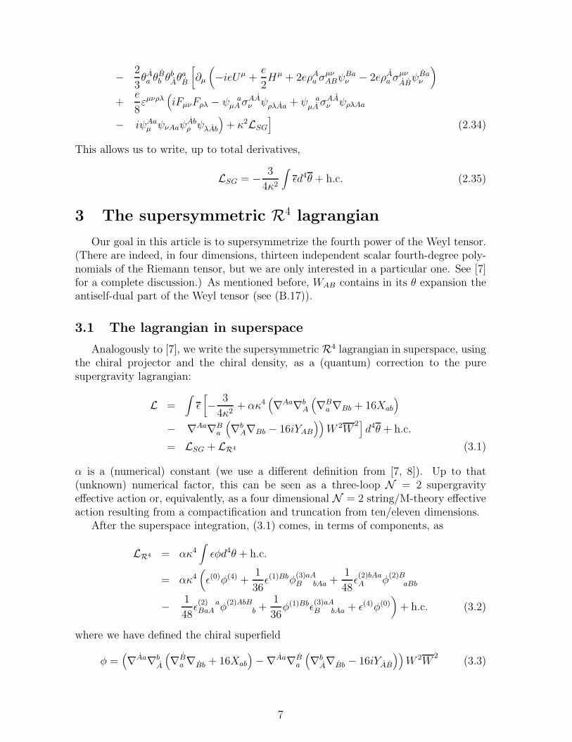
This allows us to write, up to total derivatives,

LSG = − 3

4κ2

∫ǫd4θ + h.c. (2.35)

3 The supersymmetric R4 lagrangian

Our goal in this article is to supersymmetrize the fourth power of the Weyl tensor.(There are indeed, in four dimensions, thirteen independent scalar fourth-degree poly-nomials of the Riemann tensor, but we are only interested in a particular one. See [7]for a complete discussion.) As mentioned before, WAB contains in its θ expansion theantiself-dual part of the Weyl tensor (see (B.17)).

3.1 The lagrangian in superspace

Analogously to [7], we write the supersymmetric R4 lagrangian in superspace, usingthe chiral projector and the chiral density, as a (quantum) correction to the puresupergravity lagrangian:

L =∫ǫ

[− 3

4κ2+ ακ4

(∇Aa∇b

A

(∇B

a ∇Bb + 16Xab

)

− ∇Aa∇Ba

(∇b

A∇Bb − 16iYAB

))W 2W

2]d4θ + h.c.

= LSG + LR4 (3.1)

α is a (numerical) constant (we use a different definition from [7, 8]). Up to that(unknown) numerical factor, this can be seen as a three-loop N = 2 supergravityeffective action or, equivalently, as a four dimensional N = 2 string/M-theory effectiveaction resulting from a compactification and truncation from ten/eleven dimensions.

After the superspace integration, (3.1) comes, in terms of components, as

LR4 = ακ4∫ǫφd4θ + h.c.

= ακ4(ǫ(0)φ(4) +

1

36ǫ(1)Bbφ

(3)aAB bAa +

1

48ǫ(2)bAaA φ

(2)BaBb

− 1

48ǫ(2) aBaA φ

(2)AbBb +

1

36φ(1)Bbǫ

(3)aAB bAa + ǫ(4)φ(0)

)+ h.c. (3.2)

where we have defined the chiral superfield

φ =(∇Aa∇b

A

(∇B

a ∇Bb + 16Xab

)−∇Aa∇B

a

(∇b

A∇Bb − 16iYAB

))W 2W

2(3.3)

7

and

φ(0) = φ|φ(1)Aa = ∇Aaφ

∣∣∣

φ(2)AaBb =

1

2[∇Aa,∇Bb]φ|

φ(3)AaBbCc =

1

6(∇Aa [∇Bb,∇Cc] + ∇Bb [∇Cc,∇Aa] + ∇Cc [∇Aa,∇Bb]) φ|

φ(4) =1

288∇Aa∇Bb [∇Ab,∇Ba]φ

∣∣∣ (3.4)

As one can see from the component expansions in appendix B, the term ǫ(0)φ(4) + h.c.clearly contains the fourth power of the Weyl tensor, more precisely (using the notationof [7]) eW2

+W2−.

3.2 The lagrangian in components

We now proceed with the calculation of the components of φ and analysis of itsfield content. For that, we use the differential constraints from the solution to theBianchi identities and the commutation relations listed in appendix B to compute thecomponents in (3.4). The process is straightforward but lengthy.

We start by expanding φ as

φ = W 2∇Aa∇bA∇B

a ∇BbW2 −W 2∇Aa∇B

a ∇bA∇BbW

2

− 32iW 2W2∇AaΛAa + 32iW 2ΛAa∇AaW

2

− 64iW 2(∇AaX b

a

)W BCWBCAb − 64iW 2X b

a

(∇AaW BC

)WBCAb

− 64iW 2X ba W

BC∇AaWBCAb −64

3W 2

(∇AaXab

)WABΛBb

− 64

3W 2Xab

(∇AaWAB

)ΛBb − 64

3W 2XabWAB∇AaΛBb

− 64W 2(∇a

AY AB

)W CDWCDBa − 64W 2Y AB

(∇a

AW CD

)WCDBa

− 64W 2Y ABW CD∇aAWCDBa +

64

3iW 2

(∇AaYAB

)W BCΛCa

+64

3iW 2YAB

(∇AaW BC

)ΛCa +

64

3iW 2YABW

BC∇AaΛCa (3.5)

All the terms in (3.5) can be immediately computed by using the differential relations inappendix B.2, except for the first two, which require a substantial amount of derivativesto compute.

In order to compute ∇AaW2, we use the known relation for ∇AaWCD:

∇AaW2

= 2W CD∇AaWCD = 4iW CDWCDAa −4

3WABΛB

a (3.6)

With this result, we can compute

∇Bb∇AaW2

= 4i(∇BbW

CD)WCDAa + 4iW CD∇BbWCDAa

− 4

3(∇BbWAC) ΛC

a − 4

3WAC∇BbΛ

Ca (3.7)

8

The field content implicit in these relations may be seen from the differential relationsin appendix B.2.

From (3.7), we can proceed computing:

∇Cc∇Bb∇AaW2

= 4i(∇Cc∇BbW

DE)WDEAa − 4i

(∇BbW

DE)∇CcWDEAa

+ 4i(∇CcW

DE)∇BbWDEAa + 4iW DE∇Cc∇BbWDEAa

− 4

3(∇Cc∇BbWAD) ΛD

a − 4

3(∇CcWAC)∇BbΛ

Ca

− 4

3(∇CcWAD)∇BbΛ

Da − 4

3WAD∇Cc∇BbΛ

Da (3.8)

We got some second spinorial derivatives of superfields, as expected, which we cancompute by differentiating some of the relations in appendix B.2. We list the resultsin appendix C.1.

From (3.8), we finally get

∇Dd∇Cc∇Bb∇AaW2

= −4

3(∇Dd∇Cc∇BbWAE) ΛE

a − 4

3(∇Cc∇BbWAE)∇DdΛ

Ea

+4

3(∇Dd∇BbWAE)∇CcΛ

Ea − 4

3(∇BbWAE)∇Dd∇CcΛ

Ea

−4

3(∇Dd∇CcWAE)∇BbΛ

Ea +

4

3(∇CcWAE)∇Dd∇BbΛ

Ea

−4

3(∇DdWAE)∇Cc∇BbΛ

Ea − 4

3WAE∇Dd∇Cc∇BbΛ

Ea

+4i(∇Dd∇Cc∇BbW

EF)WEF Aa + 4i

(∇Cc∇BbW

EF)∇DdWEF Aa

−4i(∇Dd∇BbW

EF)∇CcWEF Aa + 4i

(∇BbW

EF)∇Dd∇CcWEF Aa

+4i(∇Dd∇CcW

EF)∇BbWEF Aa − 4i

(∇CcW

EF)∇Dd∇BbWEF Aa

+4i(∇DdW

EF)∇Cc∇BbWEF Aa + 4iW EF∇Dd∇Cc∇BbWEF Aa(3.9)

As expected, we get some third spinorial derivatives of superfields, which we can com-pute by differentiating some of the relations from the previous section and in appendixB.2. We list the results in appendix C.2.

When a spinor derivative acts on a vector derivative of a superfield, first we commutethe two derivatives with the help of the torsions and curvatures listed in the appendixB. Then we use the gauge choices (2.5), (2.6) and (2.7) to write

∇µ| = ∇µ (3.10)

∇µ is a Lorentz and SU(2) covariant derivative. For an arbitrary superfield G we havethen

∇mG| = e µm∇µ G| −

1

2ψAa

m ∇AaG| −1

2ψAa

m ∇AaG| (3.11)

The equations we have been obtaining allow us to determine the field content of φ|, byreplacing the equations with fewer spinorial derivatives (starting from the differentialrelations in appendix B.2) in the ones with more spinorial derivatives, and by suitableindex contraction and derivative commutation.

9

This same relations (more precisely, their complex conjugates) will also be usefulfor calculating the higher θ components of φ. Other differential relations will be ne-cessary: the series of spinorial derivatives will act on φ|, which after the full componentexpansion contains much more fields (not only WAB). These fields will also be actedon by four spinorial derivatives, which we have not computed (and, as we will see nextsection, we don’t need to). The computations are straightforward, like the one we did

for W2. Rather than performing them, we prefer to deduce some of their properties,

using the results we have.

4 The field equations for the auxiliary fields

Having seen how to obtain the supersymmetric R4 lagrangian in components, weare now in a position to analyze the auxiliary field sector. Our main goal is to figureout which auxiliary fields, with this R4 correction, do not get spacetime derivatives inthe action (i.e. have an algebraic field equation and can be eliminated on-shell), andwhich do get. We start by the N = 2 case, the lagrangian of which we have beendetermining. Then we summarize the N = 1 case, which we analyzed in previousworks, and we compare the two cases.

4.1 The N = 2 case

We start by recalling that, in pure supergravity, both in N = 1 and in N = 2, theauxiliary fields are equal to 0 on-shell [20].

Just by looking at the differential relations in appendix B.2, it is immediate toconclude that, if a ∇BbWCDAa term shows up in the lagrangian, one gets derivatives of

ΦabAB

and of Um. This term shows up already in ∇Bb∇AaW2

(which shows up, by itself,

in higher θ components of φ). Dotted spinor derivatives of ΦabAB

and Um will introducethe physical superfieldsWCD,WCDAa, YCDAa and the auxiliary superfields YCD, Xab,ΛAa

(but not ΛAa). It also introduces a derivative of the superfield ρAa. These superfields

get then one derivative - ρAa actually gets two - in the term ∇Cc∇Bb∇AaW2.

Just by inspection, we expect these auxiliary fields to have derivatives. To actuallycompute the coefficient of their derivative terms is a hard task - basically it wouldbe equivalent to computing all the terms in the lagrangian, which would require anenormous amount of algebra. Fortunately, it is possible to compute their leadingderivative terms using a simple trick.

In the previous section we obtained an expression for φ| in terms of spinorial deriva-tives of superfields. To compute higher θ terms, we act on φ with undotted spinorderivatives. From (3.5) we see that these derivatives either act on W 2, WABCc, Xab,ΛCc, YAB or their spinor derivatives - giving rise to the equations we got in computing

φ|, but complex-conjugated -, or they act on four dotted spinorial derivatives of W2.

Each undotted derivative can be anticommuted with a dotted one (giving rise to a

vector derivative and curvature terms), until it finally acts in W2

- resulting 0. Thetorsion and curvature terms we get in this process, after all undotted derivatives aretaken, include other superfields like UAA, YABCc, the spinor derivatives of which weknow from computing φ|. Therefore, the higher θ terms of φ are either products of

10

terms we already know from φ|, or overall vector derivatives. Since the higher θ termsare multiplied, in the action (3.2), by a corresponding term of the chiral density, wecan integrate by parts the derivatives in the higher θ terms and have them acting inthe chiral density! Therefore, all the lower θ4−n terms in the chiral density are acted inthe action by n vector derivatives. Looking at the chiral density in (2.34), we concludethat Xab and Ymn have terms with at least two derivative in the action, and ΛAa hasterms with at least one derivative in the action. These terms cannot be eliminated byintegration by parts.

Furthermore, Um and Φabm also get derivatives in the action. The reason is the

following: the vector derivatives we get come from superspace and, therefore, are (orcan be made) Lorentz and U(2) covariant. 3 The physical theory should be only Lorentzinvariant; the U(1) and SU(2) connections should be seen respectively as the Um andΦab

m auxiliary fields. Therefore, terms with n vector (Lorentz and U(2) covariant)derivatives give rise to n− 1 vector Lorentz covariant derivatives of Um and Φab

m .Derivatives of P and Hm superfields still have not appeared up to now. By our

previous arguments, if these derivatives do not appear in φ|, they do not appear atall, since these superfields do not appear in the chiral density except in the highest θterm. Therefore, all that is left to do is check that φ| has no derivatives of ρa

A, P , theirhermitean conjugates and Hm.

4.1.1 Derivatives of P and Hm in ∇Bb∇AaW2

and ∇Cc∇Bb∇AaW2

The P and Hm superfields only appear in ∇Bb∇AaW2

through I, which belongs tothe original Weyl multiplet and is given by (2.30), and its derivatives 4. Recall that I

itself has a divergence ∇BBHBB and derivatives ∇BBρAa; it shows up already in the

expansion of ∇Bb∇AaW2

in (3.7), through ∇BbΛBb. These derivatives already show up

at this early stage, and will keep showing up as the calculation goes. We anticipate thatwe will be interested only in derivatives of fields coming from the nonlinear multiplet.Therefore, from now on when we refer to ”derivatives of Hm” we are excluding itsdivergence.

As we keep going and compute ∇Cc∇Bb∇AaW2, we see that the derivatives in which

we are interested come only from the ∇CcI term; all the other terms in (3.8), whichwe computed in terms of known expressions in appendix C.1, contribute at most with∇BBH

BB terms.The complete expansion for ∇CcI is given by (C.4) in appendix C.1. For each term

in this equation, we compute in appendix D.1 its content in terms of the derivativesof interest. Now, here a surprise happens: after all the contributions have been ana-lyzed, we conclude that they all precisely cancel in such a way that ∇CcI contains no

3In this paper, they are just SU(2) covariant, by our choice. The choice of tangent group insuperspace is a matter of convenience. We could have kept the U(2) covariance, and the argument inthe text would be valid directly, but we broke this covariance to SU(2). We get them extra Um terms- Um was the U(1) connection -, which would be reabsorbed in the derivatives, if the U(2) covariancehad been kept.

4We will be only looking for derivatives of P because, although this superfield is chiral, it isgenerated (and acquires derivatives) through ∇BbρAa and ∇BbHAA. Its complex conjugate, P , doesnot get derivatives in φ, but gets them in φ.

11

derivatives of P or of Hm (with the exception of ∇BBHBB, as before). This result is

easily obtained from (C.4) and the expressions from appendix D.1. This shows that

derivatives of P and Hm do not come up to ∇Cc∇Bb∇AaW2.

4.1.2 Derivatives of P and Hm in ∇Dd∇Cc∇Bb∇AaW2

An even bigger surprise is that these derivatives also cancel in those terms from

∇Dd∇Cc∇Bb∇AaW2

in which we will be interested. The procedure we took to fullycheck these cancellations was analogous to the previous case: we expanded each term in(3.9) in terms of known expressions in appendix C.2. For those terms which had deriva-tives of interest, we computed their derivative content in appendix D.2. We summedall the possible contributions for each term in (3.9) and we list them next. During thepartial calculations we see lots of independent terms appearing from different sources,but at the end we found several remarkable cancellations of those terms. The mostremarkable one happens in ∇Dd∇CcI, which is part of the term with ∇Dd∇Cc∇BbΛAa

in (3.9). As it can be seen from the expansion of ∇Dd∇CcI in equation (C.14), in orderto get the derivative content of this term we need contributions from every expressionin appendix D. It turns out, though, after a lot of algebra, that all the contributionsprecisely cancel in such a way that ∇Dd∇CcI has absolutely no derivatives of P or Hm

besides ∇BBHBB, exactly like ∇CcI in the previous section. All these results can be

checked using the equations in appendices C and D. After performing all the calcu-lations, the final result is then the following: the only nonvanishing contributions tointeresting derivative terms in (3.9) come from

∇Dd∇Cc∇BbWEF Aa =1

4εBAεDCεdcXab∇A

EHAF +

1

4εBAεDCεdcΦ

AEab

∇AFP + · · · (4.1)

These terms actually do not vanish in ∇Dd∇Cc∇Bb∇AaW2, but they do vanish in

φ. This is because, as it may be seen from (3.5), φ only contains the combina-

tions ∇Aa∇b

A∇B

a ∇BbW2

and ∇Aa∇Ba ∇b

A∇BbW

2. In the first combination, we need

∇Dd ∇Dc∇BcW d

EF B, while in the second we need ∇Dc∇C

c ∇bDWEF Cb. Both these com-

binations have no derivatives of interest, as one sees from (4.1).The other terms from (3.5) do not have any interesting derivatives, as it may be

easily seen from the equations in appendix B.2. We thus have shown that in φ| thereare not any derivatives of P or Hm, apart from the divergence of this last field.

4.1.3 Higher θ terms of φ

We have shown that φ| contains no derivatives of P or the transversal part of Hm.For that purpose, we needed to compute spinor derivatives of all the superfields of ”oldminimal” N = 2 supergravity. As one can see from the results of appendix D, notall spinor derivatives of superfields originate the vector derivatives we were looking at;only the spinor derivatives of the ”dangerous” superfields ρa

A, P , Hm and Φab

m originatesuch derivatives.

In order to compute the higher θ terms of φ, we act on (3.5) with undotted spinorderivatives and follow the procedure described in the beginning of this section. We willfind only terms that we have already computed but, most important, we will only find

12

spinor derivatives of the ”safe” superfields WAB, WABCc, Xab, ΛCc, YAB, UAA, YABCc, orof their spinor derivatives, but not of any of the ”dangerous” ones. These superfieldsare ”safe” even in the sense that they are ”closed” with respect to differentiation:spinor derivatives of ”safe” superfields only originate ”safe” superfields.

This way, we conclude there are no derivatives of P or the transversal part of Hm

in the N = 2 supersymmetrization of the fourth power of the Weyl tensor.

4.1.4 The behavior of ρaA

Our results indicate that in N = 2 ”old minimal” supergravity with the R4 correc-tion, the bosonic auxiliary fields from the compensating nonlinear multiplet do not getderivatives and can still be eliminated. Auxiliary fields from the Weyl (Ymn, ΛAa, Um,Φab

m) and vector (Xab) multiplets get derivatives and cannot be eliminated.The only unclear result is the behavior of the fundamental (in terms of which all the

others are defined) auxiliary field ρaA. Derivatives of ρa

A (and of its hermitian conjugate)are not generated by the process of integration by parts we mentioned, but they areconstantly being generated in the computation of φ| already from its beginning. Thisis because these derivatives exist already in the simple differential relations of appendixB.2 and in the definition (2.30) of I. This is why we have not fully calculated thesederivatives, as we did with the other superfields: that would require computing a bignumber of terms and, for each term, a huge number of different contributions. This isprobably because ρa

A belongs to a nonlinear multiplet. It would seem a miracle that allthese derivative terms would cancel, but we have not shown that they do not cancel andwe cannot rule it out! We can at least provide arguments supporting the hypothesisof cancellation. And there are at least two good ones. The first argument is that itseems strange (although it is not impossible) to have a field (ρa

A) with a dynamical fieldequation while having two fields obtained from its spinorial derivatives (P and Hm -see appendix B.1) without such an equation. The second argument is that ρa

A, like Pand Hm, are intrinsic to the ”old minimal” version of N = 2 supergravity; they allcome, as we saw, from the same multiplet. The physical theory does not depend onthese auxiliary fields and, therefore, it seems natural that they can be eliminated fromthe classical theory and its quantum corrections. We checked that P and (transversal)Hm can be eliminated; the same should be expected for ρa

A. If that was the casethat the derivatives of ρa

A would cancel, its field equation would be some functionof the ”dynamical” auxiliary fields and their derivatives, such that when replaced intheir definitions in appendix B.1, it would result in differential (i.e. dynamical) fieldequations for these fields.

4.2 The N = 1 case

The fields of N = 1 conformal supergravity multiplet are the graviton emµ , the

gravitino ψAµ and a U(1) gauge field Aµ. (The dilation gauge field Bµ can be gauged

away.) Just with these fields, the superconformal algebra closes off-shell. Each one ofthese is a gauge field; the corresponding gauge invariances must be considered whencounting the number of degrees of freedom. In particular, Aµ has 4-1=3 degrees offreedom [21, 22].

13

To obtain the ”old minimal” formulation of N = 1 Poincare supergravity [23,24], we take the superconformally invariant action of a chiral multiplet. In order tobreak the superconformal and local U(1) invariances, one must impose some constraintwhich restricts the parameters of their transformation rules to the chiral multiplet. Insuperspace this is achieved by imposing the following nonconformal torsion constraint[25]:

T mAm = 0 (4.2)

This constraint implies the known off-shell constraints and differential relationsbetween the N = 1 supergravity superfields R,Gm,WABC :

∇AR = 0 (4.3)

∇AGAB =1

24∇BR (4.4)

∇AWABC = i(∇BAG

AC + ∇CAG

AB

)(4.5)

which imply the relation

∇2R−∇2R = 96i∇nGn (4.6)

The (anti)chirality condition on R,R implies their θ = 0 components (resp. theauxiliary fields M − iN,M + iN) lie in antichiral/chiral multiplets; (4.4) shows thespin-1/2 parts of the gravitino lie on the same multiplets and, according to (4.6), sodoes ∂µAµ (because Gm| = Am).5

In previous works, we have considered a similar problem to the one in the presentpaper: supersymmetrizing the fourth power of the Weyl tensor, W2

+W2−, in the ”old

minimal” formulation of N = 1 supergravity [8]. When we took the superspace actionwhich included this term, we obtained algebraic field equations for R,R. Accordingto (4.6), ∇nGn also obbeys an algebraic equation. The auxiliary fields that belong tothe compensating multiplet can thus still be eliminated. This is not the case for theauxiliary fields which come from the Weyl multiplet (Am), as we obtained, in the samework, a differential field equation for Gm.

4.3 Possible generalizations

It would be interesting to figure out how the results we got can be generalized.Both N = 1 and N = 2 supergravities admit other minimal formulations, with diffe-rent choices of compensating multiplets and different sets of auxiliary fields. In ”newminimal” N = 1 [26], the chiral compensating multiplet is replaced by a compensa-ting tensor multiplet that still breaks conformal invariance but leaves the local U(1)invariance unbroken. In the ”new minimal” N = 2 [15], one still has the compensatingvector multiplet that breaks conformal and local U(1) invariances, but the nonlinearmultiplet is replaced by an ”improved tensor” compensating multiplet that breaks localSU(2) to local SO(2).

The obvious observation is that both in N = 1 and N = 2 the auxiliary fields fromthe tensor multiplets do not get derivatives in the supersymmetric R4 action, whilethe auxiliary fields from the Weyl (and vector in N = 2) multiplets do get. This way

5The remaining scalar off-shell degree of freedom is the trace of the metric.

14

we notice that, in the cases we analyzed, the auxiliary fields that can be eliminatedcome from multiplets which, on-shell, have no physical fields; while the auxiliary fieldsthat get derivatives come from multiplets with physical fiels on-shell (the graviton, thegravitino(s) and, in N = 2, the vector). Our general conjecture for R4 supergravity,which is fully confirmed in the ”old minimal” N = 1 case, can now be stated: theauxiliary fields which come from multiplets with on-shell physical fields cannot beeliminated, but the ones that come from compensating multiplets that, on shell, haveno physical fields, can.

This analysis should also be extended to nonminimal versions of these theories.These nonminimal versions would have fermionic auxiliary fields (also in N = 1). Thisshould be part of another project, and we leave more definite results to another work.Maybe by understanding the behavior of these fermionic auxiliary fields (and the onesin ”new minimal” N = 2) we could fully understand what in this paper we have justconjectured: the behavior of the auxiliary field ρa

A in ”old minimal” N = 2 supergravity.Possibly the computations would get easier in other versions of the N = 2 theory; thefact that they were difficult in the ”old minimal” formulation, particularly the onesconcerning ρa

A, is probably simply due to the presence of the nonlinear multiplet.A generalization of these results to N = 3, 4 Poincare supergravity theories, which

can also be seen as broken superconformal theories, is more difficult. This is becausethese theories do not have an off-shell formulation in conventional superspace. Aformulation like this could still be possible, but either in harmonic superspace or withmultiplets with central charge.

5 Conclusions

We wrote down an action containing an R4 correction to ”old minimal” N = 2supergravity. We analyzed its auxiliary field sector, and we concluded that the auxiliaryfields belonging to the Weyl and compensating vector multiplets acquire derivativeswith these correction and cannot be eliminated on-shell. We checked that all theterms with derivatives for the bosonic auxiliary fields from the compensating nonlinearmultiplets cancel; we argued that the same should be true for the fermionic auxiliaryfield from this multiplet, although we have not performed the full calculation in orderto reach a definitive conclusion.

In ”old minimal” N = 1 supergravity a similar result is valid: the auxiliary fieldfrom the Weyl multiplet cannot be eliminated on-shell with the R4 correction, whilethe ones from the chiral compensating multiplet can. We then conjectured that analo-gous results about the Weyl and compensating multiplets should be valid for the otherversions of N = 1, 2 supergravity. In general, we conjecture that auxiliary fields whichcome from multiplets with on-shell physical fields cannot be eliminated, but those onesthat come from compensating multiplets without any on shell physical fields can beeliminated. These results should help to clarify the structure of the supersymmetricR4 actions in more complicated and less understood theories, either with more super-symmetries (in d = 4) or in higher dimensions.

The direct supersymmetrization of higher order terms in 10 and 11 dimensionshas been an active topic of research, although lots of questions remain open. Some

15

superinvariants associated with the R4 term have been studied [27, 28, 29, 30, 31,32, 33], but complete supersymmetric effective actions including all the leading ordercorrections to supergravity are still lacking. In M-theory, because of the absence ofa microscopical formulation, the construction of superinvariants would be even moreimportant. Hopefully the results we have been getting in four dimensions will providesome insight for the higher dimensional theories!

Acknowledgements The author is very grateful to Martin Rocek for having sug-gested him this problem and, together with Warren Siegel, for very helpful discussions.He wishes to thank Antoine van Proeyen for correspondence and Bernard de Wit fordiscussions and for having indicated him useful references. He also wishes to thankINFN, Sezione di Bologna, for hospitality and financial support during a short visit inJanuary 2003. This work has been partially supported by NSF through grant PHY-0098527.

A N = 2 SU(2) superspace conventions

We work with standard SU(2) N = 2 superspace. We define

VM = (Vm, VAa, VBb) (A.1)

A, B are spinor indices, the algebra of which being exactly the same as the N = 1case, which is fully explained in [7, 8]. a is an internal SU(2) index, which is raisedand lowered with an SU(2)-invariant εab tensor, just like the spinor indices: T a =εabTb, Ta = T bεba. We take ε12 = 1. The basic rule of our conventions (different fromother conventions in the literature) is that we use the northwest rule in every index(spinor or SU(2)) contraction. The complex conjugation rules are

V aA = −VAa, V

Aa = V Aa , VAa = V a

A, V A

a = −V Aa, εab = εab, χAaψBb = −χAa ψBb (A.2)

All other conventions regarding spacetime metrics, the Riemann tensor, Pauli matrices,superspace torsions and curvatures are the same as in [7, 8].

B Solution to the Bianchi identities in N = 2 SU(2)

superspace

In conformal supergravity, all torsions and curvatures can be expressed in terms ofthe basic superfields WAB, YAB, UAA, Xab, their complex conjugates and their covariantderivatives. After breaking of superconformal invariance and local U(2), the basicsuperfields in the Poincare theory become the physical field WAB and the auxiliaryfield ρa

A. All torsions and curvatures can be expressed in terms of these superfields,their complex conjugates and their covariant derivatives. In sections B.1 and B.2 wepresent the definitions of these superfields, and then we list the torsions and curvatures.

16

B.1 Definitions

ρaA| is an auxiliary field; WAB|, at the linearized level, is related to the field strength

of the physical vector field Aµ. From (2.23), the complete expression is

WAB| = − i

2√

2σmn

ABFmn − YAB − i

4σmn

AB

(ψCc

m ψnCc + ψCcm ψnCc

)(B.1)

Now we present the definitions of the superfields of ”old minimal” N = 2 supergravityin terms of WAB and ρa

A. The hermitian conjugates can be easily obtained from thebasic rules in (A.2), which are valid for ∇a

A and ρaA, and the definition

WAB = WAB.

Xab =1

2

(∇Aa − 2ρAa

)ρ

b

A=

1

2

(∇Aa − 2ρAa

)ρ

bA (B.2)

YAB = − i

2

(∇a

A + 2ρaA

)ρBa (B.3)

UAA =1

4

(∇a

AρAa + ∇aAρAa + 4ρa

AρAa

)(B.4)

ΦabAA

=i

2

(∇a

Aρb

A−∇a

Aρ

bA − 4ρ

aAρ

b

A

)(B.5)

P = i∇AaρAa (B.6)

HAA = −i∇aAρAa + i∇a

AρAa (B.7)

ΛAa = −i∇Ab X

ab (B.8)

I = i∇AaΛAa − i∇AaΛAa (B.9)

WBCAa =i

2∇AaWBC − i

6(εABΛCa + εACΛBa) (B.10)

YBCAa = − i

2∇AaYBC (B.11)

WABCD =(i

4∇b

A∇Bb − 2YAB

)WCD (B.12)

WABCD =(i

4∇b

A∇Bb − 2YAB

)WCD

PABCD =i

8∇b

A∇BbYCD +i

8∇b

C∇DbYAB − YABYCD −WABWCD

− UACUBD (B.13)

R =i

4

(∇Aa∇B

a WAB + ∇Aa∇Ba WAB + i∇Aa∇b

AXab + i∇Aa∇b

AXab

)

− 2(WABYAB +W ABYAB

)− 6XabXab + 6U2 (B.14)

Xab∣∣∣ , YAB| , Um| , Φab

AA

∣∣∣ , P | , HAA| are auxiliary fields; I is a dependent field. WABCD

is symmetric in all its indices, but WABCc and YABCc are only symmetric in A,B. Inthe linearized approximation, WABCc| and YABCc| are the gravitino curls and WABCD|,

17

PABCD|, R| are the antiself-dual Weyl tensor, the traceless Ricci tensor and the Ricciscalar, respectively:

WABCc| = −1

4ψABCc + · · · (B.15)

YABCc| = −1

8ψABCc + · · · (B.16)

WABCD| = −1

8W+

µνρσσµνABσ

ρσCD + · · · (B.17)

PCDAB| =1

2σ

µ

CAσν

DB

(Rµν −

1

4gµνR

)+ · · · (B.18)

R| = −R + · · · (B.19)

B.2 Off-shell differential relations

These off-shell differential relations among superfields are direct consequences ofthe Bianchi identities and the definitions in B.1.

∇aAρ

bB =

i

4εABε

abP − εABXab − iεabYAB + 2ρb

AρaB (B.20)

∇aAρ

bB

= − i

4εabHAB − εabUAB − iΦab

AB+ 2ρb

AρaB

(B.21)

∇CcWAB = 0,∇CcWAB = 0 (B.22)

∇AaWBC = −2iWBCAa +1

3(εABΛCa + εACΛBa) (B.23)

∇AaXbc =i

3(εabΛAc + εacΛAb) (B.24)

∇AaYBC = −1

3(εABΛCa + εACΛBa) (B.25)

∇AaYBC = 2iYBCAa (B.26)

∇AaUBB = YABBa + εABWA

BAa+

2

3iεABΛBa (B.27)

∇aAP = 0,∇a

AP = 0 (B.28)

∇aAP = −8iW Ba

AB − 4

3Λa

A − 8ρBaWAB + 2PρaA + 2ρAaHAA

− 4iρAaUAA − 8∇AAρAa − 8Φab

AAρA

b (B.29)

∇aAHBB = 8iεABW

AaAB

+4

3εABΛa

B− 4εABρ

AaWAB − 4iεABρBbXba

− 2εABPρaB− 2εABρ

CaHCB + 4ρaBYAB + 2iρa

AUBB

− 8ρAbΦabBB

+ 8ρBbΦabAB

− 4∇BBρaA + 8∇ABρ

aB (B.30)

∇aAΦbc

BB= 2iεABε

abWAc

BA+

2

3εABε

abΛc

B− 2εABε

abρAcWAB

+ 2iεabYc

ABB− 2εabYABρ

c

B+ iεabρ

cAUBB − 2iεabρ

cBUAB

− 4εabρAdΦdc

BB− 2εab∇BBρ

cA − 2iεABX

abρc

B+ 2ρ

bAΦ

ac

BB(B.31)

18

∇aAΛb

B =i

8IεABε

ab +3

2εABε

ab∇CCUCC

+3

2iεABε

ab(Y CDWCD − Y CDWCD

)− 6YABX

ab (B.32)

∇aAΛb

B= 3iεab

(∇BBW

BA + ∇ A

A YAB

)− 3∇ABX

ab − 6iUABXab (B.33)

∇BbWCDAa = εbaWCDAB +1

12εba (εACεBD + εADεBC)R− εBA∇C

CΦCbDa

+ iεbaεCA∇CDUCB + 2εBAWCDEbρ

Ea − 2εBAYCDEbρ

Ea

+ εBAΦCeCb

ΦCeDa + 2εbaYCBWDA + εbaεCBεDAWCDYCD

+ εbaεCBεDAX2 + εbaεCBεDAU

2 + 2iεDAYCBXba

+ 2iεCBWDAXba (B.34)

∇BbWCDAa = εab∇BAWCD + εabεAC∇ BB WBD − εabεAC∇C

DYBC

+ iεAC∇BDXab − 2εACUBDXab + iεabUBAWCD

+ 2iεabεACUB

B WBD (B.35)

∇BbYCDAa = εbaPCDBA + iεba∇CAUDB − εBA∇ CC ΦDaCb

− 2εBAWCDEbρEa + 2εBAYCDEbρ

Ea + εBAΦ Ce

Cb ΦDaCe

+ εbaWCDWBA + εbaYCDYBA − εbaεBAWE

C YED

− iεBAXabYCD + iεBAXabWCD + εbaUCAUDB (B.36)

∇BbYCDAa = εbaεBC∇ CD WCA − εba∇DAYBC + iεBC∇DAXab

− iεbaYCDUBA + 2iεbaYBCUDA + 2εBCUDAXba (B.37)

∇EeWABCD = −2iεEC∇ECYABEe − 4iYECWABDe − 8εECX

fe WABDf

+ 3εECYABEeUED− 2iWABEeYCD (B.38)

∇AaWABCD = 2i∇ACWABDa + UACWABDa + 4iWCDYABAa (B.39)

∇EePCDBA = 2i∇CEYABDe − i∇CAYEBDe + iεEB∇CAWE

DE e − 2iYCDEeYAB

− iYEAYCDBe + iεEAWE

C YEDBe − 2iWCDWABEe

− iεEAWCDWC

BC e− 5εEAX

fe YCDBf − 2εEAWCDFeU

FB

+ εEAUCBWE

DE e +1

2UCBYEADe + 2UCEYABDe (B.40)

∇AaR = −i∇BBYABBa + 3i∇BAW C

BC a + 10XabWBb

AB− 2iW B

CB aY C

A

− 4iWCBAaYCB − 3iWCBYCBAa +

9

2UBBYABBa +

9

2UB

AW C

BCa(B.41)

Using (B.36) and (B.37), one may compute ∇BBYABBa; replacing in (B.41), we get themore convenient expression

∇AaR = 4i∇BAW C

BC a + 12XabWBb

AB− 2iWCBYCBAa

− 6iWCBAaYCB + 12UBBYABBa + 4UB

AW C

BC a (B.42)

19

B.3 Torsions

T abmAB

= −2iεabσmAB

T abmAB , T abm

AB= 0

TAaBbCc, TAaBbCc = 0

TAaBbCc, TAaBbCc = 0

T amnA , T amn

A= 0

TAABbCc = − i

2εbc (εABUCA + εACUBA)

TAABbCc =i

2εbc (εABUAC + εACUAB)

TAABbCc = −εbc (εABWAC + εACYAB) − iεABεACXbc

TAABbCc = εbc (εACYAB + εABWAC) + iεACεABXbc

Tmnp = 0

TAABBCc = −εABWABCc − εABYABCc

TAABBCc = εABWABCc + εABYABCc (B.43)

B.4 Lorentz curvatures

RAaBbCD = −2iεABεabYCD + 2 (εACεBD + εADεBC)Xab

RAaBbCD = −2iεABεabWCD

RAaBbCD = −2iεABεabWCD

RAaBbCD = −2iεABεabYCD + 2 (εACεBD + εADεBC)Xab

RAaBbCD = εab (εBCUDA + εBDUCA)

RAaBbCD = −εab (εACUBD + εADUBC)

RAABbCD = −iεBCYADAb + iεABYCDAb +i

2(εACεBD + εADεBC)W B

AB b

RAABbCD = iεACYABDb + 2iεABWACDb +i

3εABεACW

BD Bb

RAABbCD = iεACYABDb + 2iεABWACDb +i

3εABεACW

BD Bb

RAABbCD = −iεBCYADAb + iεABYCDAb +i

2(εACεBD + εADεBC)W B

AB b

RAABBCD = εABPCDAB +1

12εAB (εACεBD + εADεBC)R + εABWABCD

RAABBCD = εABPABCD +1

12εAB (εACεBD + εADεBC)R + εABWABCD (B.44)

B.5 SU(2) curvatures

RAaBbcd = −2εAB (εbdXac − εadXbc) − 2i (εacεbd + εadεbc)YAB

RAaBbcd = −2εAB (εbdXac − εadXbc) − 2i (εacεbd + εadεbc)YAB

20

RAaBbcd = −2 (εacεbd + εadεbc)UAB

RAABbcd = 2iεbdYABAc − 2iεABεbdWB

AB c− 2

3εABεbdΛAc

RAABbcd = 2iεbdYABAc − 2iεABεbdWB

AB c −2

3εABεbdΛAc

RAABBcd = −2εAB

(WABEcρ

Ed − YABEcρ

Ed +

1

2∇ E

A ΦBEcd −1

2Φ Ee

A cΦBEde

)

+ 2εAB

(WABEcρ

Ed − YABEcρ

Ed − 1

2∇E

AΦEBcd +

1

2ΦE

AceΦ e

EBd

)

We see that all torsions and curvatures can be expressed in terms of the basic su-perfields WAB, YAB, UAA, Xab, their complex conjugates and their covariant derivatives(see section B.1). This is obvious except for RAABBcd, which may be rewritten as

RAABBcd = εAB

(1

2∇C

cYABCd + iXcdYAB − iXcdWAB

)

+ εAB

(1

2∇C

cYABCd + iXcdYAB − iXcdWAB

)(B.45)

C The lagrangian in components

C.1 Calculation of ∇Cc∇Bb∇AaW2

In this section, we fully express the terms with two spinorial derivatives arising inthe calculation of (3.8) as functions of those with one spinorial derivative, previouslycomputed in appendix B. These terms are:

∇Cc∇BbWAD = 2i∇CcWADBb −2

3εBA∇CcΛDb (C.1)

∇Cc∇BbWDEAa = −εab∇CcWDEAB − 2εab

(∇CcYBD

)WEA − 2εabYBD∇CcWEA

+ 2εBA

(∇CcWDEFa

)ρF

b − 2εBAWDEF a∇CcρFb

− 2εBA

(∇CcYDEEa

)ρE

b + 2εBAYDEEa∇CcρEb − εBA∇Cc∇E

DΦEEab

+ 2εBAΦE eD a

∇CcΦEEeb − 2iεBD (∇CcXab)WEA

− 2iεBDXab∇CcWEA +1

6εabεEAεBD∇CcR

− iεabεEA∇Cc∇EDUEB + εabεEAεBDU

F F∇CcUF F

+ 2iεEA

(∇CcYBD

)Xab + 2iεEAYBD∇CcXab

+ εabεEAεBDWAB∇CcYAB + 2εabεEAεBDX

de∇CcXde (C.2)

∇Cc∇BbΛAa =i

8εabεBA∇CcI −

3

2εabεBA∇Cc∇F FUF F − 3

2iεabεBAW

AB∇CcYAB

+3

2iεabεBAW

EF∇CcYEF +3

2iεabεBAY

EF∇CcWEF + 6Xab∇CcYBA

+ 6YBA∇CcXab (C.3)

21

For (C.3) we need ∇CcI, which we compute here.

∇CcI = 4∇CcR− 48Xab∇CcXab − 12WAB∇CcYAB − 12W AB∇CcYAB

− 12Y AB∇CcWAB − 24UF F∇CcUF F + 3P∇CcP + 3HF F∇CcHF F

− 24ΦF Fab ∇CcΦ

abF F

− 6∇Cc∇F FHF F − 16i(∇Ccρ

Aa)

ΛAa + 16iρAa∇CcΛAa

+ 16i(∇Ccρ

Aa)

ΛAa − 16iρAa∇CcΛAa + 48(∇Ccρ

Aa)W B

AB a

− 48ρAa∇CcWB

AB a − 48(∇Ccρ

Aa)W B

AB a+ 48ρAa∇CcW

BAB a

− 96iWABρAa∇CcρaB − 96iW ABρAa∇Ccρ

aB

+ 48iρAaρaB∇CcW

AB

− 48UAA (∇CcρAa) ρaA

+ 48UAAρAa∇CcρaA− 48ρAaρ

aA∇CcU

AA

+ 48i (∇CcρAa)∇AAρaA− 48iρAa∇Cc∇AAρa

A− 48i (∇CcρAa)∇AAρa

A

+ 48iρAa∇Cc∇AAρaA + 96iΦab

AAρA

b ∇CcρAa + 96iΦab

AAρA

b ∇CcρAa

+ 96iρAa ρ

Ab ∇CcΦ

abAA

(C.4)

Terms involving combinations of vector and spinor covariant derivatives may be writ-ten as vector derivatives of the relations listed in appendix B using the commutationrelations.

C.2 Calculation of ∇Dd∇Cc∇Bb∇AaW2

In this section, we fully express the terms with two and three spinorial derivativesarising in the calculation of (3.9) as functions of those with one spinorial derivative,previously computed in appendix B. These terms are:

∇Dd∇Cc∇BbWEF = 2i∇Dd∇CcWEF Bb −2

3εBE∇Dd∇CcΛF b (C.5)

∇Dd∇Cc∇BbWEF Aa = −εab∇Dd∇CcWEF AB − 2εab

(∇Dd∇CcYBE

)WF A

+ 2εab

(∇CcYBE

)∇DdWF A − 2εab

(∇DdYBE

)∇CcWF A

− 2εabYBE∇Dd∇CcWF A + 2εBA

(∇Dd∇CcWEF Ga

)ρG

b

+ 2εBA

(∇CcWEF Ga

)∇Ddρ

Gb − 2εBA

(∇DdWEF Ga

)∇Ccρ

Gb

+ 2εBAWEF Ga∇Dd∇CcρGb − 2εBA

(∇Dd∇CcYEFEa

)ρE

b

− 2εBA

(∇CcYEFEa

)∇Ddρ

Eb + 2εBA

(∇DdYEFEa

)∇Ccρ

Eb

− 2εBAYEFEa∇Dd∇CcρEb − εBA∇Dd∇Cc∇E

EΦEFab

+ 2εBAΦE eE a

∇Dd∇CcΦEFeb − 2εBA

(∇CcΦ

E eE a

)∇DdΦEFeb

− iεabεEA∇Dd∇Cc∇EFUEB + εabεEAεBF

(∇DdU

GG)∇CcUGG

+ εabεEAεBFUGG∇Dd∇CcUGG − 2iεBE (∇Dd∇CcXab)WF A

+ 2iεBE (∇CcXab)∇DdWF A − 2iεBE (∇DdXab)∇CcWF A

− 2iεBEXab∇Dd∇CcWF A − 2iεAE (∇Dd∇CcXab)YF B

22

+ 2iεAE (∇CcXab)∇DdYF B − 2iεAE (∇DdXab)∇CcYF B

− 2iεAEXab∇Dd∇CcYF B + εabεEAεBFWAB∇Dd∇CcYAB

+ 2εabεEAεBF

(∇DdX

ef)∇CcXef + 2εabεEAεBFX

ef∇Dd∇CcXef

+1

6εabεEAεBF∇Dd∇CcR (C.6)

∇Dd∇Cc∇BbΛAa = −3

2εabεBA∇Dd∇Cc∇F FUF F − 3

2iεabεBAW

AB∇Dd∇CcYAB

+3

2iεabεBA

(∇DdW

EF)∇CcYEF +

3

2iεabεBAW

EF∇Dd∇CcYEF

+3

2iεabεBA

(∇DdY

EF)∇CcWEF +

3

2iεabεBAY

EF∇Dd∇CcWEF

+ 6 (∇DdXab)∇CcYBA + 6Xab∇Dd∇CcYBA + 6YBA∇Dd∇CcXab

+ 6 (∇DdYBA)∇CcXab +i

8εabεBA∇Dd∇CcI (C.7)

These results require knowing second spinorial derivatives of superfields, some ofwhich we have computed in section C.1, but others we have not computed yet. Wepresent those here:

∇Dd∇CcWEF AB = −4i(∇DdYBA

)WBEF c − 4iYBA∇DdWBEF c

− 8εCF (∇DdXe

c )WABEe − 8εCFXe

c ∇DdWABEe

− 2i(∇DdYAB

)WEF Cc − 2iYAB∇DdWEF Cc − 2iεCF∇Dd∇E

EYABEc

+ 3εCF

(∇DdU

EE

)YABEc + 3εCFU

EE∇DdYABEc (C.8)

∇Dd∇CcρBb = −εCB∇DdXcb − iεcb∇DdYBC + 2ρBc∇DdρCb − 2ρCb∇DdρBc (C.9)

∇Dd∇CcρBb =i

4εcb∇DdHBC − εcb∇DdUBC + i∇DdΦBCcb + 2ρBc∇DdρCb

− 2ρCb∇DdρBc (C.10)

∇Dd∇CcYABAa = εac∇Dd∇AAYCB + 2iεac

(∇DdUAA

)YCB + 2iεacUAA∇DdYCB

− iεac (∇DdUAC)YAB − iεacUAC∇DdYAB − εacεCB∇Dd∇BAWAB

+ iεCB∇Dd∇AAXac − 2εCB

(∇DdUAA

)Xac

− 2εCBUAA∇DdXac (C.11)

∇Dd∇CcΦBBba = 2iεbcεBC∇DdWA

BA a +2

3εbcεBC∇DdΛBa + 2εbcεBC

(∇Ddρ

Aa

)WAB

− 2iεbc∇DdYBCBa + 2εcb

(∇DdρBa

)YBC − 2εcbρBa∇DdYBC

− iεcb

(∇DdρCa

)UBB + iεcbρCa∇DdUBB + 2iεcb

(∇DdρBa

)UBC

− 2iεcbρBa∇DdUBC + 4εcb

(∇Ddρ

eC

)ΦBBea − 4εcbρ

eC∇DdΦBBea

− 2εcb∇Dd∇BBρCa − 2iεBC

(∇DdρBb

)Xca + 2iεBCρBb∇DdXca

+ 2(∇DdρCb

)ΦBBca − 2ρCb∇DdΦBBca (C.12)

∇Dd∇CcUBB = −∇DdYBCBc − εBC∇DdWA

AB c +2

3iεBC∇DdΛBc (C.13)

23

∇Dd∇CcR = 4i∇Dd∇BCW A

BA c + 12 (∇DdXcb)WBb

CB+ 12Xcb∇DdW

BbCB

− 2iWCB∇DdYCBCc − 6i (∇DdWABCc)YAB + 6iWABCc∇DdY

AB

+ 12(∇DdU

BB)YCBBc + 12UBB∇DdYCBBc + 4

(∇DdU

BC

)W C

BC c

+ 4UBC∇DdW

CBC c

∇Dd∇CcI = 4∇Dd∇CcR− 48(∇DdX

ab)∇CcXab − 48Xab∇Dd∇CcXab

− 12WAB∇Dd∇CcYAB − 12(∇DdW

AB)∇CcYAB

− 12W AB∇Dd∇CcYAB − 12(∇DdY

AB)∇CcWAB

− 12Y AB∇Dd∇CcWAB − 24(∇DdU

F F)∇CcUF F

− 24UF F∇Dd∇CcUF F + 3P∇Dd∇CcP + 3(∇DdH

F F)∇CcHF F

+ 3HF F∇Dd∇CcHF F − 24(∇DdΦ

F Fab

)∇CcΦ

abF F

− 24ΦF Fab ∇Dd∇CcΦ

abF F

− 6∇Dd∇Cc∇F FHF F

− 16i(∇Dd∇Ccρ

Aa)

ΛAa − 16i(∇Ccρ

Aa)∇DdΛAa

+ 16i(∇Ddρ

Aa)∇CcΛAa − 16iρAa∇Dd∇CcΛAa

+ 16i(∇Dd∇Ccρ

Aa)

ΛAa + 16i(∇Ccρ

Aa)∇DdΛAa

− 16i(∇Ddρ

Aa)∇CcΛAa + 16iρAa∇Dd∇CcΛAa

+ 48(∇Dd∇Ccρ

Aa)W B

AB a + 48(∇Ccρ

Aa)∇DdW

BAB a

− 48(∇Ddρ

Aa)∇CcW

BAB a + 48ρAa∇Dd∇CcW

BAB a

− 48(∇Dd∇Ccρ

Aa)W B

AB a− 48

(∇Ccρ

Aa)∇DdW

BAB a

+ 48(∇Ddρ

Aa)∇CcW

BAB a

− 48ρAa∇Dd∇CcWB

AB a

− 96iWAB (∇DdρAa)∇CcρaB + 96iWABρAa∇Dd∇Ccρ

aB

− 96i(∇DdW

AB)ρAa∇Ccρ

aB− 96iW AB (∇DdρAa)∇Ccρ

aB

+ 96iW ABρAa∇Dd∇CcρaB− 96iρAa

(∇Ddρ

aB

)∇CcW

AB

+ 48iρAaρaB∇Dd∇CcW

AB − 48 (∇Dd∇CcρAa) ρaAUAA

− 48UAA (∇CcρAa)∇DdρaA

+ 48 (∇CcρAa) ρaA∇DdU

AA

+ 48(∇DdU

AA)ρAa∇Ccρ

aA

+ 48UAA (∇DdρAa)∇CcρaA

− 48UAAρAa∇Dd∇CcρaA− 48 (∇DdρAa) ρ

aA∇CcU

AA

+ 48ρAa

(∇Ddρ

aA

)∇CcU

AA − 48ρAaρaA∇Dd∇CcU

AA

+ 48i (∇Dd∇CcρAa)∇AAρaA

+ 48i (∇CcρAa)∇Dd∇AAρaA

− 48i (∇DdρAa)∇Cc∇AAρaA

+ 48iρAa∇Dd∇Cc∇AAρaA

− 48i (∇Dd∇CcρAa)∇AAρaA − 48i (∇CcρAa)∇Dd∇AAρa

A

+ 48i (∇DdρAa)∇Cc∇AAρaA − 48iρAa∇Dd∇Cc∇AAρa

A

24

+ 96i(∇DdΦ

abAA

)ρA

b ∇CcρAa + 96iΦab

AA

(∇Ddρ

Ab

)∇Ccρ

Aa

− 96iΦabAAρA

b ∇Dd∇CcρAa + 96i

(∇DdΦ

abAA

)ρA

b ∇CcρAa

+ 96iΦabAA

(∇Ddρ

Ab

)∇Ccρ

Aa − 96iΦab

AAρA

b ∇Dd∇CcρAa

+ 96i(∇Ddρ

Aa

)ρA

b ∇CcΦabAA

− 96iρAa

(∇Ddρ

Ab

)∇CcΦ

abAA

+ 96iρAa ρ

Ab ∇Dd∇CcΦ

abAA

(C.14)

Because of the ∇Dd∇CcI term in ∇Dd∇Cc∇BbΛAa, we will also need the followingterms:

∇Dd∇CcP = −8i∇DdWB

CB c− 4

3∇DdΛCc + 8

(∇Ddρ

Bc

)WCB − 8ρB

c ∇DdWCB

+ 2(∇DdP

)ρCc + 2P∇DdρCc + 2

(∇Ddρ

Cc

)HCC − 2ρC

c ∇DdHCC

+ 4i(∇Ddρ

Cc

)UCC − 4iρC

c ∇DdUCC − 8∇Dd∇CCρCc

+ 8 (∇DdΦCCcb) ρCb + 8ΦCCcb∇Ddρ

Cb (C.15)

∇Dd∇CcHBB = 8iεCB∇DdWA

AB c +4

3εCB∇DdΛBc + 4εCBWBC∇Ddρ

Cc

− 4iεCBXbc∇DdρbB + 4iεCBρ

bB∇DdXbc − 2εCBP∇DdρBc

− 2εCBHBA∇DdρAc + 2εCBρ

Ac ∇DdHBA − 4YCB∇DdρBc

+ 4ρBc∇DdYCB − 2iUBB∇DdρCc + 2iρCc∇DdUBB

+ 8ΦBBbc∇DdρbC− 8ρb

C∇DdΦBBbc − 4∇Dd∇BBρCc

+ 8∇Dd∇BCρBc + 8ρbB∇DdΦBCbc − 8ΦBCbc∇Ddρ

bB

(C.16)

∇Dd∇CcΛBb = 3iεcb∇Dd∇BBWB

C+ 3iεcb∇Dd∇A

CYAB − 3∇Dd∇BCXcb

+ 6i (∇DdUBC)Xcb + 6iUBC∇DdXcb (C.17)

∇Dd∇CcWABCc = −εcb∇Dd∇ACWBC + 2iεcb

(∇DdUAC

)WBC − εcbεBC∇Dd∇ B

A YBC

− iεBC∇Dd∇ACXcb − iεcb (∇DdUCC)WAB − 2εBC

(∇DdUAC

)Xcb

− 2εBCUAC∇DdXcb (C.18)

∇Dd∇CcYAB = 2i∇DdYABCc (C.19)

∇Dd∇CcYAB =2

3εCB∇DdΛAc (C.20)

∇Dd∇CcXab = −2

3iεca∇DdΛCb (C.21)

All other differential relations we will need involve combinations of vector and spinorcovariant derivatives. Terms containing these expressions are very important for ouranalysis, since a lot of the derivatives we are looking for come from them. They may bewritten, using the commutation relations, as vector derivatives of the relations we haveseen plus torsion and curvature terms. Some of the torsion terms require differentialrelations involving undotted and dotted spinorial derivatives which we compute now:

∇aA∇c

Cρb

B= − i

4εCBε

cb∇aAP − εCB∇a

AXcb − iεcb∇a

AYCB + 2ρcB∇a

AρbC

− 2ρbC∇a

AρcB

(C.22)

25

∇aA∇c

Cρb

B =i

4εcb∇a

AHBC − εcb∇aAUBC + i∇a

AΦbcBC

+ 2ρcB∇a

AρbC

− 2ρbC∇a

AρcB (C.23)

∇dD∇c

CHBB = 8iεCB∇d

DWCc

BC +4

3εCB∇d

DΛcB + 4εCBWBC∇d

DρCc

− 4εCBρCc∇d

DWBC + 4iεCBXcb∇d

DρCb − 4iεCBρ

Cb ∇d

DXcb

− 2εCBρcB∇d

DP − 2εCBP∇dDρ

cB − 2εCBHBA∇d

DρAc

+ 2εCBρAc∇d

DHBA − 4YCB∇dDρ

cB + 4ρc

B∇dDYCB − 2iUBB∇d

DρcC

+ 2iρcC∇d

DUBB − 8ΦbcBB

∇dDρCb + 8ρCb∇d

DΦbcBB

+ 8ΦbcBC

∇dDρBb

− 8ρBb∇dDΦbc

BC− 4∇d

D∇BBρcC

+ 8∇dD∇BCρ

cB

(C.24)

∇Dd∇CcUBB = −∇DdYCBBc + εCB∇DdWC

BC c −2

3iεCB∇DdΛBc (C.25)

∇dD∇c

CΦab

BB= 2iεCBε

cb∇dDW

CaBC +

2

3εCBε

cb∇dDΛ

aB + 2εCBε

cbWBC∇dDρ

Ca

− 2εCBεcbρCa∇d

DWBC + 2iεcb∇dDY

a

CBB+ 2εcbYCB∇d

DρaB

− 2εcbρaB∇d

DYCB − iεcbUBB∇dDρ

a

C+ iεcbρ

a

C∇d

DUBB + 2iεcbUBC∇dDρ

a

B

− 2iεcbρa

B∇d

DUBC + 2iεCBXcb∇d

DρaB − 2iεCBρ

aB∇d

DXcb + 2Φ

bc

BB∇d

Dρa

C

− 2ρa

C∇d

DΦbc

BB− 4εcbΦ

ae

BB∇d

DρCe + 4εcbρCe∇dDΦ

ae

BB− 2εcb∇d

D∇BBρa

C

(C.26)

All these expressions should be enough for the direct computation of (3.9).

D Calculation of the derivative terms

In this appendix, we compute the terms arising in the calculation of ∇Cc∇Bb∇AaW2

and ∇Dd∇Cc∇Bb∇AaW2

which contain vector derivatives of the auxiliary fields P,Hm

(excluding ∇mHm, as justified on the text). For each expression, we indicate its contentin terms of the derivatives of interest. The derivatives of some of these expressions willalso be necessary; for those expressions, we give their field content in terms of P,Hm.Through all this appendix, we will be only interested in the derivatives we mentionedand, therefore, we will only consider here expressions which contain them. Thoseexpressions we do not consider here simply do not contain such derivatives, as it canbe verified using their expansions in appendix C.

D.1 Calculation of the derivative terms in ∇Cc∇Bb∇AaW2

From (3.8), the following expressions are necessary:

∇cC∇b

BWDE =

i

4εbcεDBεEC

(PP +H2 − 2∇AAH

AA)

+ · · · (D.27)

∇cC∇b

BW a

DEA= − i

2εBAε

acPWb

DEC+i

2εBAε

acHECYEb

DE+ · · · (D.28)

∇bB∇AAρ

cC

= − i

4εbcεBC∇AAP +

i

4εbcYABHAC +

i

4εbcεABW

DA HDC

26

− 1

4εACε

bcPUAB +1

8εbcεBCPUAA − 1

4εABX

bcHAC + · · · (D.29)

∇cC∇AAρ

Aa =i

4εca∇AAH

AC− i

2εcaPYAC +

1

2εACPX

ca

− 1

8εcaUAAH

AC

+1

4εcaUACH

AA

+ · · · (D.30)

∇AA∇bBHCC = 2εCBρ

bC∇AAP + 2εCBP∇AAρ

bC + 2εCBρ

Db∇AAHCD

+ 2εCBHCD∇AAρDb + · · · (D.31)

D.2 Calculation of the derivative terms in ∇Dd∇Cc∇Bb∇AaW2

In order to compute the derivatives in (3.9), besides the previous expressions wealso need

∇dD∇c

CP = −2iεdc∇CCH

CD

+ · · · (D.32)

∇dD∇c

CHBB = 2iεdcεBC∇BDP − 2εBCX

cdHBD − iεDCεdcW C

B HCB

− iεDCεdcY A

BHBA + 4iεdcHBBYCD + · · · (D.33)

∇dD∇c

CHBB = −iεdcεCBεDB∇AAH

AA + iεdc∇BBHDC − 2iεdc∇BCHDB

+ · · · (D.34)

∇dD∇AA∇c

CHBB = iεCBεABε

dcYAD∇EEHEE − iεdcYAD∇BBHAC

+ 2iεdcYAD∇BCHAB + iεCBεADεdcWAB∇EEH

EE

− iεADεdcW C

A ∇BBHCC + 2iεADεdcW C

A ∇BCHCB

− εCBεADεABXdc∇EEH

EE + εADXdc∇BBHAC

− 2εADXdc∇BCHAB − εBCε

dcUAA∇BDP − εCAεdcUAD∇BBP

+ 2εBAεdcUAD∇BCP + 2iεBCε

dc∇AA∇BDP

− iεDCεdcW C

B ∇AAHCB − 2εBCXdc∇AAHBD

− iεDCεdcY E

B∇AAHBE + 4iεdcYCD∇AAHBB + · · · (D.35)

∇dD∇c

C∇AAHBB = ∇d

D∇AA∇c

CHBB − iεDBεABε

dcYAC∇EEHEE + iεdcYAC∇BBHAD

− 2iεdcYAC∇ABHBD − iεdcεDBεACWAB∇EEHEE

+ iεdcεACWC

A ∇BBHCD − 2iεdcεACWC

A ∇CBHBD

− εABεDBεACXdc∇EEH

EE

+ εACXdc∇BBHAD − 2εACX

dc∇ABHBD

− εdcεBCUAA∇BDP + 2εdcεBDUAC∇BAP + · · · (D.36)

Remarkably, when we contract the A,B and A, B indices, lots of terms in the previousequations cancel by themselves. Ignoring the ∇EEH

EE parts, in which we are notinterested, we are simply left with

∇dD∇c

C∇AAH

AA = 4εdcUAC∇ADP + · · · (D.37)

27

We also need more derivatives of ρbB:

∇aA∇c

Cρb

B= − i

2εcbεCBρ

aAP − i

2εcbHABρCa −

i

2εCBε

abHAAρAc

− i

2εCBε

cbHAAρAa + · · · (D.38)

∇dD∇c

C∇AAρ

bB

= − i

2εdbεDCρ

cB∇AAP +

i

2εdcεDBρ

bC∇AAP + · · · (D.39)

∇dD∇c

C∇AAρ

bB = −iεcbεDCρ

cB∇AAP − i

2εcbεDCρ

Bd∇AAHBB

− i

2εdcρb

C∇AAHBD + · · · (D.40)

With respect to derivatives of ΦabAB

, we need:

∇dD∇c

CΦab

BB=

i

2εCBε

caεdbW AB HAD +

i

2εDBε

caεdbW AB HAC +

i

2εcaεdbYBCHBD

− i

2εcaεdbYBDHBC − 1

2εCBε

dbXcaHBD − 1

2εDBε

cbXdaHBC

− iεcaεDCΦdb

BBP − i

2εdaεDCΦ

cb

BBP +

i

2εcaεdbεDC∇BBP + · · ·(D.41)

∇dD∇c

CΦab

BB=

i

2εcaεdb∇BBHDC + · · · (D.42)

∇dD∇c

C∇AAΦab

BB=

i

2εcaεdbεDC∇AA∇BBP

− iεcaεDCΦdb

BB∇AAP − i

2εdaεDCΦ

cb

BB∇AAP

− i

2εCBε

caεdbW DB ∇AAHDD +

i

2εDBε

caεdbW DB ∇AAHDC

− i

2εCAε

caεdbW DA ∇BBHDD +

i

2εDAε

caεdbW DA ∇BBHDC

+i

2εcaεdbYBC∇AAHBD − i

2εcaεdbYBD∇AAHBC

− i

2εcaεdbYAC∇BBHAD +

i

2εcaεdbYAD∇BBHAC

− 1

2εCBε

dbXca∇AAHBD − 1

2εDBε

cbXda∇AAHBC

− 1

2εCAε

dbXca∇BBHAD +1

2εDAε

cbXda∇BBHAC + · · · (D.43)

We did not include in (D.41) and (D.43) those terms with a UAA∇BBP factor, simplybecause these terms exist in partial calculations, but overall they cancel. The termwith ∇AA∇BBP does not cancel in (D.43), but this expression appears in (C.6) as∇d

D∇c

C∇B

AΦab

BB. Therefore, this term appears as ∇B

A∇BBP , a commutator that does

not have vector derivatives.Replacing all the appropriate expressions in (C.14), with suitable contraction or

symmetrization of the adequate indices, and adding all terms, we are led to the sur-prising and exciting result that ∇Dd∇CcI, like ∇CcI, also has no derivatives of P,HAA

other than ∇AAHAA. We analyze the other terms from (3.9) in the main text.

28

References

[1] S. Deser, J.H. Kay and K.S. Stelle: Phys. Rev. Lett. 38 (1977), 527.

[2] M. B. Green and J. H. Schwarz: Phys. Lett. 149B (1984), 117.

[3] M. B. Green and J. H. Schwarz: Phys. Lett. 151B (1985), 21; idem, Nucl. Phys.

B255 (1985), 93.

[4] D. J. Gross and E. Witten: Nucl. Phys. B277 (1986), 1.

[5] D. J. Gross and J. H. Sloan: Nucl. Phys. B291 (1987), 41.

[6] M. T. Grisaru, A. E. M. van de Ven and D. Zanon: Phys. Lett. 173B (1986), 423;idem, Nucl. Phys. B277 (1986), 388; idem, Nucl. Phys. B277 (1986), 409; M. T.Grisaru and D. Zanon: Phys. Lett. 177B (1986), 347.

[7] F. Moura: J. High Energy Phys. 08 (2002), 038, hep-th/0206119.

[8] F. Moura: J. High Energy Phys. 09 (2001), 026, hep-th/0106023.

[9] S.J. Gates, Jr.: Nucl. Phys. B176 (1980), 397; idem, Phys. Lett. 96B (1980), 305.

[10] P. Howe: Nucl. Phys. B199 (1982), 309.

[11] M. Muller: Consistent Classical Supergravity Theories, Lecture Notes in Physics,Springer-Verlag, 1989.

[12] M. Muller: Nucl. Phys. B289 (1987), 557.

[13] B. de Wit and J.W. van Holten: Nucl. Phys. B155 (1979), 530.

[14] P. Breitenlohner and M.F. Sohnius: Nucl. Phys. B178 (1981), 151.

[15] B. de Wit, R. Philippe and A. van Proeyen: Nucl. Phys. B219 (1983), 143.

[16] M. Muller: Nucl. Phys. B282 (1987), 329.

[17] B. de Wit, J. W. van Holten and A. van Proeyen: Nucl. Phys. B167 (1980), 186;idem, Nucl. Phys. B184 (1981), 77.

[18] E.S. Fradkin and M.A. Vasiliev: Lett. Nuovo Cim. 25 (1979), 79; idem, Phys.

Lett. 85B (1979), 47.

[19] M. Muller: Phys. Lett. 172B (1986), 353.

[20] M. Muller: Zeit. fur Phys. C24 (1984), 175.

[21] M. Kaku, P.K. Townsend and P. van Nieuwenhuizen: Phys. Lett. 69B (1977), 304;idem, Phys. Rev. Lett. 39 (1977), 1109; idem, Phys. Rev. D17 (1977), 3179.

[22] P. van Nieuwenhuizen: Supergravity, Phys. Rep. 68C (1981), 189.

29

[23] K. Stelle and P. West: Phys. Lett. 74B (1978), 330.

[24] S. Ferrara and P. van Nieuwenhuizen: Phys. Lett. 74B (1978), 333.

[25] P. Howe and R.W. Tucker: Phys. Lett. 80B (1978), 138.

[26] M.F. Sohnius and P. West: Phys. Lett. 105B (1981), 353.

[27] B. E. W. Nilsson and A. L. Tollsten: Phys. Lett. 171B (1986), 212.

[28] M. de Roo, H. Suelmann and A. Wiedemann: Nucl. Phys. B405 (1992), 326,hep-th/9210099.

[29] S. de Haro, A. Sinkovics and K. Skenderis: Phys. Rev. D67:084010 (2003),hep-th/0210080.

[30] K. Peeters, P. Vanhove and A. Westerberg: Class. Quant. Grav. 18 (2001), 843,hep-th/0010167; idem, hep-th/0010182.

[31] M. Cederwall, U. Gran, M. Nielsen and B. E. W. Nilsson: J. High Energy Phys.

10 (2000), 041, hep-th/0007035; idem, hep-th/0010042.

[32] S. J. Gates, Jr. and H. Nishino: Phys. Lett. 508B (2001), 155, hep-th/0101037.

[33] H. Nishino and S. Rajpoot: Phys. Rev. D64 (2001), 124016, hep-th/0103224.

30