arX

iv:h

ep-t

h/97

0415

1v1

21

Apr

199

7

hep-th/9704151RU-97-12, CU-TP-823, IASSNS-HEP-97/24

Orbifold Resolution by D-Branes

Michael R. Douglas,1 Brian R. Greene,2,∗ and David R. Morrison3,†

1Department of Physics and Astronomy

Rutgers University

Piscataway, NJ 08855–0849

mrd@physics.rutgers.edu

2Departments of Physics and Mathematics

Columbia University

New York, NY 10025

greene@math.columbia.edu

3Schools of Mathematics and Natural Sciences

Institute for Advanced Study

Princeton, NJ 08540

drm@math.duke.edu

We study topological properties of the D-brane resolution of three-dimensional orbifold

singularities, C3/Γ, for finite abelian groups Γ. The D-brane vacuum moduli space is

shown to fill out the background spacetime with Fayet–Iliopoulos parameters controlling

the size of the blow-ups. This D-brane vacuum moduli space can be classically described

by a gauged linear sigma model, which is shown to be non-generic in a manner that

projects out non-geometric regions in its phase diagram, as anticipated from a number of

perspectives.

April 1997

∗ On leave from Department of Physics, Cornell University, Ithaca, NY 14850.† On leave from Department of Mathematics, Duke University, Durham, NC 27708-0320.

1. Introduction

D-branes are interesting probes of topology and geometry—as explored in many recent

works, spacetime is a derived concept from the D-brane perspective, emerging from non-

trivial moduli spaces of D-brane world-volume gauge theories.

Orbifold resolution was the first non-trivial example of this phenomenon, studied

in [1,2,3]. The classical Lagrangian of the probe theory is a projection of maximally

supersymmetric super Yang–Mills theory, with Fayet–Iliopoulos terms controlled by twist

sector moduli. In the two dimensional case— C2/Γ —it was shown that the classical gauge

theory moduli space is the resolved orbifold, and the metric is computable. The result is

a physical realization of the hyper-Kahler quotient construction of Kronheimer [4].

Here we demonstrate that an analogous procedure works for cyclic orbifold singu-

larities in three complex dimensions, treating the simplest examples C3/Z3 and C3/Z5

explicitly. The world-volume theory has the equivalent of d = 4, N = 1 supersymme-

try, and the superpotential and D-terms are no longer related by supersymmetry. The

mathematical counterpart of this statement is that the construction is not a hyper-Kahler

quotient but rather a blow-up of a singular Kahler quotient. The superpotential defines

the complex structure and the blow-up, while the D-terms define the periods of the metric

(though the full metric depends on both data). The resulting theories are physical realiza-

tions of a generalization of Kronheimer’s construction to Cn/Γ orbifold resolution, recently

developed by Sardo Infirri [5,6].

In this note we discuss topological and qualitative aspects of the construction. We

show that a generic deformation of the moduli from the orbifold point leads to complete

resolution of the orbifold and produces a smooth metric.

At weak string coupling, where our analysis is directly applicable, D-branes provide a

description of spacetime at short distances complementary to the closed string approach

of [7,8,9]. In that approach, it was found that the Kahler moduli spaces of sigma model

compactification form but a small subset of the possibilities. Linear sigma models—when

available—provide a more general definition and reveal a rich phase structure of the moduli

space including target spaces of different topology and non-geometric phases. Computa-

tions using mirror symmetry established that all of these phases are connected, and gave

physical results suggesting a more geometrical picture even for the non-geometric phases.

By using D-brane gauge theory, we can study topological properties of orbifolds on

length scales r in the range l11p < r <√

α′. The classical physics of these probe theories

1

turns out to also be describable by gauged linear sigma models, and a priori, the moduli

space of these linear sigma models could again have numerous phases. We show, though,

that the D-brane linear sigma models are not generic in that they only probe part of

the linear sigma model moduli space. We present evidence that this subspace is nothing

but the “partially enlarged Kahler moduli space,” every point of which has a geometrical

interpretation. Thus D-branes appear to directly project out the non-geometric phases.

We believe that this D0-brane description remains qualitatively correct even at strong

string coupling, following the lines of [10,11,12]. (This issue will be discussed further in

[13].) If so, our results confirm an idea of Witten that in M theory only geometric phases

appear [14].

In section 2, we review some relevant aspects of the stringy description of the moduli

space of Calabi–Yau compactification. In section 3 we discuss the D-brane construction.

In section 4 we derive some of the qualitative features the moduli spaces, using the gauged

linear sigma model description. Section 5 gives conclusions and some open questions.

2. Quantum geometry of Calabi–Yau manifolds

At present there are two limits near which one can understand the quantum moduli

space of Kahler structures on a Calabi–Yau manifold: weakly coupled IIa (or IIb) string

theory and M theory. As the explicit analysis we carry out is justified in the weak string

coupling limit, we first describe our work in the IIa framework; subsequently, we comment

on its possible relevance in M theory, assuming unexpected surprises do not arise when

extrapolating to strong coupling.

The starting point is a classical moduli space of metrics on a Calabi–Yau manifold

M . This is locally a product of a space of complex structures MC and complexified

Kahler forms MK . Classically, MK is a complexification of the Kahler cone MKc, the

subset of H2(M, R) for which the volumes of cycles are positive. As such, it appears to

have boundaries, each of which requires physical explanation. A priori these explanations

would be expected to involve quantum effects, and this is the subject of quantum geometry.

For our present purpose it is worthwhile to build up to the quantum corrected version

of MKc in two steps. First, one must augment the complexification of MKc to Mp.e.Kc , the

partially enlarged Kahler moduli space, which consists of the classical complexified Kahler

cones of all Calabi–Yau manifolds related to M by flops along rational curves, glued along

common faces. Second, realizing that this does not exhaust the full moduli space [7,8],

2

one must augment Mp.e.Kc by gluing on additional regions (or “phases”) which arise when

higher dimensional subspaces of M or its birational cousins are shrunk to points.

Quantum corrections can also change the boundaries between different phases. In

weakly coupled string theory, these changes are by effects of order α′. Thus it may be that

even in a phase in which a cycle shrinks to a point, its observed volume is non-zero.

The final result is sometimes called the enlarged nonlinear sigma model Kahler moduli

space Me.n.Kc , though it is already a good description of MK at weak string coupling.

There are two approaches to carrying out the second step. One can seek a mirror

manifold W of M and study its complex structure moduli space using standard techniques

from algebraic geometry, or one can seek a gauged linear sigma model description of M .

Each has its advantages and disadvantages. The linear sigma model approach allows us

to physically identify all of the additional regions in Me.n.Kc . These are usually called

“non-geometrical phases” since they are not interpretable in terms of smooth Calabi–Yau

sigma models. Instead, they are most naturally described in terms of more abstract field

theories such as orbifolds, Landau–Ginsburg models, and various hybrid combinations.

However, unlike the mirror symmetry approach, the linear sigma model does not construct

Me.n.Kc directly. Rather, it builds an auxiliary moduli space—the enlarged linear sigma

model moduli space Me.l.Kc. The latter is discussed in detail in [8] as well as [7,9,15,16];

it fills out all of H2(M, C), for example. The space Me.l.Kc must then be subjected to a

renormalization group action in order to yield the moduli space Me.n.Kc for conformally

invariant physical models. In other words, the linear sigma model parameters mapped

out by Me.l.Kc are secondary constructs which can be used to label universality classes of

physical string models; their primary physical counterparts, however, are the parameters

which arise upon passing to the conformal limit.

Of course, regardless of which approach one follows, the final form for Me.n.Kc is the

same. The essential properties of Me.n.Kc for our present concerns are three-fold. First, Me.n.

Kc

has numerous phase regions, some of which have a manifest geometric interpretation in

terms of Calabi–Yau nonlinear sigma models, while others do not. The boundaries in Me.n.Kc

are not sharp phase transitions but rather delineate the edges of perturbative convergence

in each region. One can pass from region to region by analytic continuation. Second, the

boundaries of the classical geometrical moduli space Mp.e.Kc get shifted by terms of order α′

in the quantum corrected moduli space Me.n.Kc . Third, Me.n.

Kc appears to be a subset of the

classical moduli space Mp.e.Kc . This inclusion has not been proven, but strong circumstantial

evidence has been presented in [9]. Assuming it to be true, we learn that every point in

3

Me.n.Kc either has a geometrical or analytically continued geometrical interpretation. For

instance, a Landau–Ginsburg, hybrid or orbifold phase can be interpreted as the analytic

continuation of a smooth Calabi–Yau sigma model, beyond the realm of sigma model

perturbation theory, (i.e., to distance scales on the order of√

α′).

As D-branes are natural probes of sub-stringy distance scales, it is important to un-

derstand the geometrical structure they sense at such points in moduli space. D-brane

geometry arises in a different manner from the traditional fundamental string approach.

Whereas a classical background geometry is generally introduced in fundamental string

theory and then subjected to various corrections, D-brane geometry emerges from the

study of the D-brane vacuum moduli space. In general this space also undergoes quantum

corrections, but in the particular case of D0-branes at weak string coupling, these are

suppressed. Thus the geometry can be accessed through a classical study of the vacuum

structure of a world volume super-Yang–Mills theory.

In our present study of orbifold resolution, this world-volume theory will turn out

to be classically describable as a gauged linear sigma model, which would seem to fit

well with the fundamental string description above. However, closer inspection reveals a

crucial difference: the linear sigma model describing D-branes is not the one usually used

to study fundamental strings. Now in the fundamental string context, it did not really

matter which linear sigma model was used as a starting point. Only properties of the

conformally invariant limit were observable, and a central ingredient in this analysis was

the associated use of the renormalization group to pass to the conformally invariant limit.

It was this process that gave an analytically continued geometrical interpretation to the

“non-geometric” phases. For D-branes there is no analogous step. If the D-brane linear

sigma model analysis were to yield non-geometric phases, we would have to live with them.

In the following sections we shall see that the D-brane linear sigma model differs from

that arising from fundamental strings in just the right way to yield a compatible spacetime

interpretation while avoiding the non-geometric phases. At least in the orbifold examples

we study, spacetime at short distances as probed by D-branes agrees with the analytically

continued geometry probed by fundamental strings. In a novel fashion, D-branes avoid the

non-geometrical phases.

What happens if we try to extrapolate this picture to large string coupling? In the

M theory limit, the string scale is far below the eleven-dimensional Planck scale, leading

to the conjecture that additional quantum effects vanish [14]. Specifically, in [14] it was

argued that the non-geometric phases in the type IIa vector multiplet moduli space are

4

squeezed to zero size. What this means is that the geometrical phases contained in Me.n.Kc

—the conformal limit of Mp.e.Kc —expand to fill out the region delineated by the classical

counterpart, Mp.e.Kc , while the non-geometrical phases are flattened out to constitute the

boundaries. In other words, all physical models again have a geometrical interpretation,

except now we do not even have to perform analytic continuation to find it. This is

precisely in accord with our D-brane picture which avoids non-geometrical phases from

the word go. In this sense, the strong coupling extrapolation of our analysis confirms part

of the M-theory picture of [14]. It would very interesting to extend this analysis to the

other “non-geometrical” phases such as Landau–Ginsburg models and hybrids and see if

the same conclusion follows.

An important conclusion of [9] is that conformal field theory orbifold points have a

nonzero B-field. This implies, as pointed out in [17], that wrapped D2-branes and D4-

branes have nonzero mass at the deep interior point of an orbifold phase. On the other

hand, there are boundary points of the orbifold phase where the quantum volume of cycles

associated with the singularity do vanish, and it is here that wrapped D-branes become

massless. In the strong string coupling limit, as the orbifold phase gets squeezed, the

conformal field theory orbifold point and the singular boundary point coincide.1 The

wrapped D-branes at the non-singular orbifold point should become massless in this limit.

We can explicitly see this in our D-brane analysis by identifying wrapped states with

“fractional” D-brane configurations. We will show that the masses of these states go to

zero as 1/gs in the strong string coupling limit.

3. C3/Γ orbifold compactification

We consider a type II string theory compactified on C3/Γ, with Γ a Zn subgroup of

SU(3). We take n odd to get an isolated singularity. It is well known that these orbifolds

can be resolved to smooth spaces with b3 = 0; in the simplest example of C3/Z3 this is

just a blow-up replacing the singularity with a P2. As it happens, in the general case

b2 = b4 = (n − 1)/2.

We take complex coordinates Zi and a generator g of Zn labeled by three integers

(a1, a2, a3) with a1 + a2 + a3 ≡ 0 (mod n). It acts as Zi → ωaiZi with ω ≡ exp 2πi/n.

Thus the unbroken d = 4 supersymmetry will be N = 2 in the closed string sector, and

N = 1 on the D-branes.

1 This can also seen by analyzing the orbifold point directly in M theory compactified on the

product of S1 with a three-dimensional orbifold [18,19].

5

3.1. Closed string spectrum

The closed string sector has n − 1 twist sectors. In type II theory each contains a

complex NS-NS field φk, and a complex R-R field making up a hyper (IIb) or vector (IIa)

multiplet. There is a reality condition [20]

φn−k = φ∗k (3.1)

leaving (n − 1)/2 complex NS-NS fields. These are the fields which in the large volume

limit become the complexified Kahler forms B + iJ on the resolution. The R-R fields in

the kth twisted sector are a complex bispinor in d = 4 satisfying the same reality condition.

These decompose into complex p-form potentials C(p)k , where the GSO projection enforces

two properties (see for example [21,22]): first, p must be even for IIb and odd for IIa,

and second, dC(p)k = i ∗ dC

(2−p)k . These p-form potentials correspond in the large volume

limit to integrals of the bulk R-R fields over various cycles. In IIb, these are∫Σ2

C(2) and∫Σ4

C(4+) (since the fields∫Σ2

C(4+) are redundant due to the self-duality of C(4+)), while

in IIa, they are∫Σ2

C(3) (whose duals are of the form∫Σ4

C(5)).

The type I spectrum is the subsector of type IIb surviving the Ω (world-sheet twist)

projection. This removes the B moduli, leaving k NS-NS moduli to control the real Kahler

forms, and k R-R scalars.

3.2. D-brane theory

On physical grounds, we expect type II compactification on the large volume limit of

a Calabi–Yau to contain the same Dp-branes as the uncompactified theory, with D-branes

wrapped about supersymmetric cycles giving BPS states.

As curvatures approach the string scale, stringy corrections to the world-volume La-

grangians of these branes could become important. For example, a single D0-brane will

have a world-volume kinetic term incorporating a metric gµν which, although Ricci-flat in

the small curvature limit, a priori need not be, just as the superstring sigma model met-

ric satisfies a modified Einstein equation with corrections of order O(α′3). The D0-brane

metric need not be exactly equal to the string metric and at this writing explicit results

for these metrics have not been obtained. However it seems likely that such corrections

are present.

Conformal field theory provides a more general language for compactification, and D-

branes in this general context have been discussed in [23]. It is a very interesting question

6

whether moduli spaces of superconformal boundary conditions are always similar to the

geometric moduli spaces of the sigma model D-branes.

Here we discuss D-branes defined on an orbifold and related theories obtained by

adding twisted sector moduli with small coefficients, following the approach of [1] in two

complex dimensions. The basic results we rely on are, first, an analysis of world-sheet

consistency conditions which shows that the orbifold prescription of closed string theory

also applies to open string theory, with all new “open string twisted sectors” provided

by adding images of the original D-branes.2 Second, analyticity of conformal perturbation

theory around the orbifold point guarantees that the D-brane world-volume Lagrangian will

be the projected flat space Lagrangian with corrections analytic in the blowup parameters.

Thus a Dirichlet p-brane at a point in C3/Γ will be defined as the quotient of the

theory of n Dirichlet p-branes in C3 by a combined action of Γ on C3 and the D-brane

index (Chan–Paton factor). A single Dirichlet p-brane is described by taking the Chan–

Paton factors in the regular representation of Γ. It is also possible to consider other

representations as in [11] (intuitively, leaving out some of the images) as we discuss below.

The D-brane theory on C3 is dimensionally reduced d = 4, N = 4 supersymmetric

gauge theory with gauge group U(n). The generator g now acts as above on C3 and on

the Chan–Paton factors as the regular representation, γ(g)ij = δijωi. The gauge field

projection is

Ai,j = ωi−jAi,j (3.2)

leaving the subgroup U(1)n unbroken.

The complex positions are the bosonic components of chiral multiplets. They must

satisfy

Xµi,j = ωi−j+aµXµ

i,j . (3.3)

Thus, the non-zero fields take the form Xµi,i+aµ

, and each such field is charged under two

U(1)’s. All fields are uncharged under the diagonal U(1).

The action on the fermions is determined the same way, but now taking g to act on

spinors. For Γ ⊂ SU(3), the N = 4 gaugino will decompose in the N = 1 theory into a

singlet (partners of (3.2)) and triplet (partners of (3.3)). For Γ 6⊂ SU(3), the projection

will generally lead to a non-supersymmetric theory.

2 The essential features of this analysis can be found in [24] and [1]; related issues are treated

in [25] and references therein. We also thank T. Banks and M. Berkooz for discussions on this

topic.

7

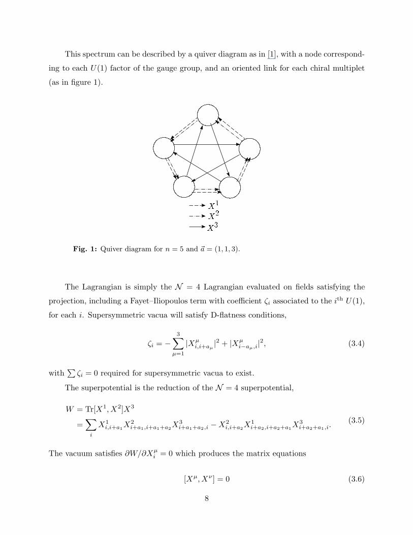
This spectrum can be described by a quiver diagram as in [1], with a node correspond-

ing to each U(1) factor of the gauge group, and an oriented link for each chiral multiplet

(as in figure 1).

X1X2X3Fig. 1: Quiver diagram for n = 5 and ~a = (1, 1, 3).

The Lagrangian is simply the N = 4 Lagrangian evaluated on fields satisfying the

projection, including a Fayet–Iliopoulos term with coefficient ζi associated to the ith U(1),

for each i. Supersymmetric vacua will satisfy D-flatness conditions,

ζi = −3∑

µ=1

|Xµi,i+aµ

|2 + |Xµi−aµ,i|2, (3.4)

with∑

ζi = 0 required for supersymmetric vacua to exist.

The superpotential is the reduction of the N = 4 superpotential,

W = Tr[X1, X2]X3

=∑

i

X1i,i+a1

X2i+a1,i+a1+a2

X3i+a1+a2,i − X2

i,i+a2X1

i+a2,i+a2+a1X3

i+a2+a1,i.(3.5)

The vacuum satisfies ∂W/∂Xµi = 0 which produces the matrix equations

[Xµ, Xν ] = 0 (3.6)

8

or in components,

X1i,i+a1

X2i+a1,i+a1+a2

= X2i,i+a2

X1i+a2,i+a2+a1

X2i,i+a2

X3i+a2,i+a2+a3

= X3i,i+a3

X2i+a3,i+a3+a2

X3i,i+a3

X1i+a3,i+a3+a1

= X1i,i+a1

X3i+a1,i+a1+a3

.

(3.7)

Although naıvely there are 3n− 3 conditions, which combined with the n− 1 quotients by

U(1) would eliminate the (Higgs branch) moduli space, these conditions are not transverse

to one another and thus the solution to (3.7) can be a non-trivial variety, which we denote

by N~a. For example, it is easy to verify that with no Fayet–Iliopoulos terms, the Higgs

branch N~a//U(1)n−1 coincides with C3/Zn, e.g. by taking Xµ = xµγ(g)aµ.

The Fayet–Iliopoulos coefficients ζi control the metric on moduli space, and as in

[1] this means they should be controlled by twisted moduli. The computation of these

couplings in the appendix of [1] can be extended to this case. The main point is the role

of the Chan–Paton twist γ(g) in the amplitude—a coupling to the sector twisted by gk

corresponds to a world-sheet amplitude with an insertion of γ(gk) at the end-point of the

cut produced by the closed string twist field. The couplings between the R-R fields and

gauge field strengths on the branes are then easy to compute, while the Fayet–Iliopoulos

terms are the supersymmetric partners. This leads (in the example of the IIb D1-brane,

with the other Dp-branes being analogous) to couplings of the form

n−1∑

k=1

∫d2x C

(2)k Tr γ(gk) + C

(0)k Tr γ(gk)F + φk Tr γ(gk)D (3.8)

where F is the matrix of gauge field strengths (satisfying the projection γ(g)Fγ(g)−1 = F),

and D the corresponding matrix of auxiliary fields. Since γ(gk)ii = ωik, the coupling

involves a discrete Fourier transform. In the Z3 example, we have φ2 = φ∗1 and the

coefficients of the D-terms become

ζi = ωiφ1 + ω2iφ∗1

which satisfy∑

ζi = 0 and see both real and imaginary parts of φ1, in other words, both

J and B.

9

3.3. “Fractional branes” and wrapped branes

As discussed in [11], world-sheet consistency conditions do not require the image

D-branes to fill out the regular representation of Γ. Even if we start with the regular

representation, when the images sit at the fixed point, there are flat directions which

separate them in the non-compact space (the Coulomb branch) [2]. Thus if we claim

that the orbifold resolution is geometric, we must find a geometric interpretation for these

states.

Let us consider the world-volume theories associated with the one-dimensional rep-

resentations of Γ. Specifically, for each k, 1 ≤ k ≤ n, we can consider the representation

γ(k) defined by γ(k)(g)ij = δikδjkωk. The orbifold projection removes the transverse co-

ordinates and the only surviving matter is the position in the non-compact space, so this

theory describes an object bound to the fixed point. Its mass and charge can be deter-

mined by doing world-sheet computations of the one-point function of the metric or R-R

string vertex operators, and the leading term comes from a disk diagram with boundary

on the D-brane. The dependence on the representation γ is the factor Tr(γi) in the ith

twisted sector as in (3.8).

Since each image couples equally to the metric, in conventions where a conventional

(regular representation) brane has mass 1/gs, a single image has mass 1/ngs. This is exact

at the orbifold point, while turning on background fields can modify the mass, as we discuss

shortly. Similarly, in conventions where the R-R charge of a conventional brane is 1, the

brane associated with the kth representation has charge ωik/n for the R-R field in the ith

twisted sector. This is the same discrete Fourier transform which appears in the gauge field

couplings and it is simpler to think of the kth representation as associated with the kth

U(1) in the quiver diagram, and work with R-R fields in the Fourier transform basis as well.

The scalars in this basis control Fayet–Iliopoulos parameters; as above the kth and (n−k)th

scalar control B and J for the kth two-cycle. Thus the kth brane is charged under the R-R

fields associated with the kth (or (n−k)th) two-cycle and four-cycle. (This discussion is

closely related to the generalized McKay correspondence which holds for arbitrary finite

subgroups of SU(3) [26,27].)

The natural interpretation of all this is that the kth “fractional brane” is actually a

Dirichlet (p+ℓ)-brane, wrapped around an ℓ-cycle implicit in the orbifold theory, to produce

a Dp-brane in the lower dimensional theory (or a bound state of such branes) [2,11].

Further confirmation of this can be found by considering the supersymmetric partners

10

of these couplings. For example, turning on the Fayet–Iliopoulos parameter ζi for the

U(1) associated with the brane increases its mass by ζ2i /ngs, the only term in the D-term

potential surviving the projection. On the other hand, the brane still has the same fermion

zero modes and corresponds to an object in the same supermultiplet, so the result must

be a mass for the brane consistent with the central charge formula.

In gauge theory terms, turning on ζi eliminates the supersymmetric vacua on the

Higgs branch; however the supersymmetry breaking is of a trivial form, a constant shift of

the Hamiltonian. This must be associated with a central charge and it would be interesting

to make this precise.

These results for the masses are controlled at weak string coupling and for small

blow-up parameter |ζ| << α′. For |ζ| ∼ α′, we would expect them to be modified by

corrections to the D-brane world-volume Lagrangian analytic in ζ/α′, defined in principle

by string world-volume computation. The phase boundary between orbifold and non-linear

sigma model phases [7] might find a counterpart here in the domain of convergence of this

expansion.

In the Z3 example, the three elementary wrapped branes have charges (1, 0),

(−12 ,√

3/2) and (−12 ,−

√3/2) under the real and imaginary parts of C

(p)1 . In a more

natural charge basis, the charges of the three states are (1 0), (0 12) and (−1 − 1

2); not

having computed the kinetic term for C(p)1 , the normalization of these charges is undeter-

mined, so we might as well use this basis.

In IIa theory, we could consider “fractional” zero-branes; what states are these con-

nected to in the large radius limit? Zero-branes can come from wrapped D2-branes,

wrapped D4-branes or bound states of these objects. These objects are electrically and

magnetically charged (respectively) under the U(1) associated with the two-cycle. Evi-

dently the first object is the wrapped two-brane and the second two are wrapped four-

branes; the electric charge of the wrapped four-branes comes from the expectation value for

B and the coupling∫

C(2)∧(F −B). The symmetry between the two wrapped four-branes

fits well with the known value B = 12 at the orbifold point [9].

The masses 1/ngs of the elementary fractional branes implicitly determine the Kahler

modulus A =∫

B + iJ at the orbifold point, as well as its special geometry partner F ′(A)

determining the masses of magnetically charged states. For example, the mass spectrum

of the C3/Z3 case suggests that the gauge coupling is τ = e2πi/3, which is natural as the

R-R gauge field coupling does not depend on gs.

11

All of these masses can also be determined by mirror symmetry techniques [9,28],

though not all of these predictions have been made explicit yet; for example the masses of

wrapped four-branes (currently under investigation). Completing this comparison, besides

confirming these identifications, would give a microscopic explanation of the masses of

wrapped branes. Symmetries which can only exist in quantum geometry, such as the Z3

acting on the wrapped two-branes and four-branes of our example, would also be given an

explicit microscopic picture.

Besides the elementary branes associated with one-dimensional representations, the

general theory of this form can contain bound states at threshold, which will correspond

to wrapped branes of higher degree. Such branes are expected to exist at large volume

[14] and it will be interesting to identify these as well.

3.4. Further corrections to the world-volume Lagrangian

In the case of C2/Γ considered in [1], supersymmetry determined the kinetic term in

the D-brane world-volume Lagrangian, preventing other dependence on the twist fields φi.

(See [12] for further discussion, especially of the case of several D0-branes.) In the present

case, this is no longer true. The configuration space can have a non-trivial metric, as long

as it is asymptotically flat and reduces to the flat metric for φi = 0. In principle, it can be

determined at weak string coupling by explicit world-sheet computation, again along the

lines of [1].

The metric could also get corrections in the string loop expansion. For general p-

branes, these could be important even at weak string coupling, due to world-volume IR

effects (i.e., renormalization). However, for D0-branes, the dynamics are governed by a non-

singular quantum mechanical theory of heavy objects, and as such, IR effects are controlled

by the masses of the world-volume degrees of freedom, which in turn are determined by

the blow-up parameters ζ. Thus the loop expansion will be controlled by the parameter

gs/ζ3/2. For blow-ups which are large compared to the eleven-dimensional Planck scale

but small compared to the string scale, these effects are small, justifying the classical

description.

On the other hand, these corrections are uncontrolled in the strong coupling limit, and

the bare metric must be regarded as undetermined. Thus, the definition of M theory on

an orbifold advocated in [11], as the strong coupling limit of the D0-brane theory (which

if interpreted following the proposal of [10] could give a complete definition of M theory

in this background), is not fully explicit for C3/Γ.

12

This is an important point because the simplest version of the construction—namely,

to use the flat metric for the D-brane gauge theory configuration space—appears to disagree

with physical expectations. M theory for low energy processes on manifolds of small

curvature (R ≪ 1/l2pl) reduces to supergravity, and thus one might expect the low energy

configuration space in the problem at hand to have a Ricci-flat metric. The classical

treatment (which can be justified for D0-branes in this regime) produces the metric as a

Kahler quotient, which on general grounds has no reason to be Ricci-flat. Indeed, Sardo

Infirri has argued that in the example of C3/Z3, the relevant metric is not Ricci-flat [5].

One possible resolution of this discrepancy is that the bare metric might not be flat.3

Another is that bound states of large numbers of D0-branes see an effective metric which is

Ricci flat. These issues will be discussed in [13] and [30], but for present purposes, when we

make statements about M theory, we are assuming that some form of the D0-brane system

defined here, in particular with a non-singular kinetic term, is a correct representation of

the strong coupling limit. This will allow us to make certain topological and even geometric

statements.

4. Geometrical interpretation

In this section we shall consider the topological properties of the D-brane vacuum

moduli space. Since sub-string scale spacetime emerges from this moduli space, we an-

ticipate that the construction just outlined is geometrically interpretable as C3/Γ with

the smoothing of its singularities being controlled by the Fayet–Iliopoulos parameters. As

we reviewed, previous studies have shown [7,8], though, that perturbative string theory

probes a rich phase structure associated with an orbifold background. For various choices

of the blow-up parameters, the resulting configuration can be any of a number of bira-

tionally equivalent but topologically distinct smooth Calabi–Yau spaces, partially resolved

orbifolds, Landau–Ginzburg orbifolds, or hybrids which mix these possibilities. From the

perspective of perturbative string theory all of these distinct backgrounds smoothly join on

to one another as the Fayet–Iliopoulos parameters are varied. By interpreting the D-brane

vacuum moduli space as an effective spacetime background, we will be able to determine

the fate of these phases at ultra-short distances.

The classical D-brane moduli space, for fixed values of the Fayet–Iliopoulos parame-

ters, is obtained by imposing the superpotential (3.7) and D-term constraints (3.4), and

3 A similar phenomenon has recently been observed in an analogous context [29].

13

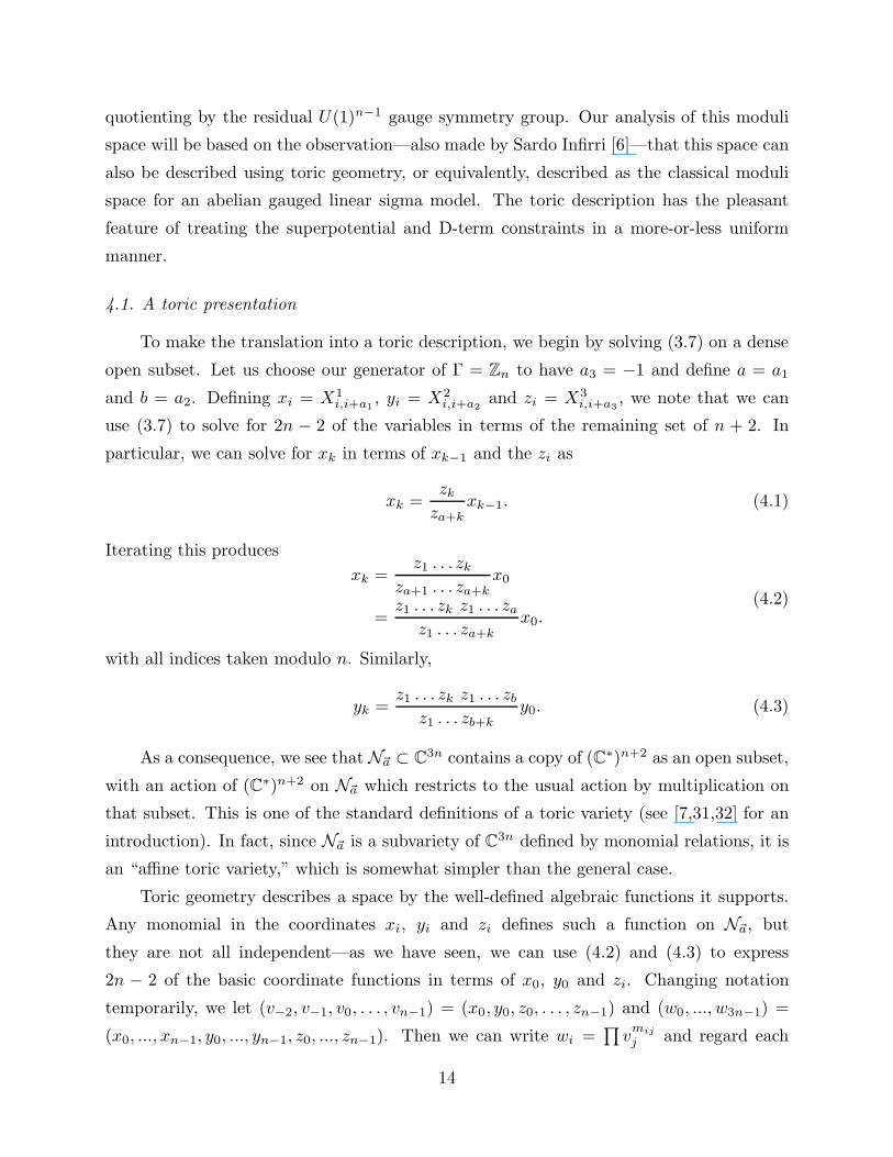
quotienting by the residual U(1)n−1 gauge symmetry group. Our analysis of this moduli

space will be based on the observation—also made by Sardo Infirri [6]—that this space can

also be described using toric geometry, or equivalently, described as the classical moduli

space for an abelian gauged linear sigma model. The toric description has the pleasant

feature of treating the superpotential and D-term constraints in a more-or-less uniform

manner.

4.1. A toric presentation

To make the translation into a toric description, we begin by solving (3.7) on a dense

open subset. Let us choose our generator of Γ = Zn to have a3 = −1 and define a = a1

and b = a2. Defining xi = X1i,i+a1

, yi = X2i,i+a2

and zi = X3i,i+a3

, we note that we can

use (3.7) to solve for 2n − 2 of the variables in terms of the remaining set of n + 2. In

particular, we can solve for xk in terms of xk−1 and the zi as

xk =zk

za+kxk−1. (4.1)

Iterating this produces

xk =z1 . . . zk

za+1 . . . za+kx0

=z1 . . . zk z1 . . . za

z1 . . . za+kx0.

(4.2)

with all indices taken modulo n. Similarly,

yk =z1 . . . zk z1 . . . zb

z1 . . . zb+ky0. (4.3)

As a consequence, we see that N~a ⊂ C3n contains a copy of (C∗)n+2 as an open subset,

with an action of (C∗)n+2 on N~a which restricts to the usual action by multiplication on

that subset. This is one of the standard definitions of a toric variety (see [7,31,32] for an

introduction). In fact, since N~a is a subvariety of C3n defined by monomial relations, it is

an “affine toric variety,” which is somewhat simpler than the general case.

Toric geometry describes a space by the well-defined algebraic functions it supports.

Any monomial in the coordinates xi, yi and zi defines such a function on N~a, but

they are not all independent—as we have seen, we can use (4.2) and (4.3) to express

2n − 2 of the basic coordinate functions in terms of x0, y0 and zi. Changing notation

temporarily, we let (v−2, v−1, v0, . . . , vn−1) = (x0, y0, z0, . . . , zn−1) and (w0, ..., w3n−1) =

(x0, ..., xn−1, y0, ..., yn−1, z0, ..., zn−1). Then we can write wi =∏

vmij

j and regard each

14

~mi ∈ M = Zn+2 as a vector of exponents. A general monomial will now be associated

with a point in M given by a sum of these basis vectors with non-negative integer coeffi-

cients. The set of all such points will form a cone M+ ⊂ M .

Conversely, a basis for the algebra of functions on N~a determines the space N~a. The

cone M+ determines such an algebra and basis—each point in the cone gives us a basis

vector, and the multiplication law is induced from addition in Zn+2.

Since we can reconstruct N~a from the cone M+, we can use any description of the

cone to define the space. Another description is in terms of a set of hyperplanes which

bound the cone, i.e., vectors ~n for which

~n · ~m ≥ 0. (4.4)

These vectors are points in the dual lattice N ∼= Hom(M, Z). Clearly the sum of two

solutions ~n of (4.4) will also satisfy (4.4) for all M+, so this condition defines a dual cone

N+ ⊂ N . Given N+, the original cone M+ can be reconstructed, so the space N~a can also

be specified by a choice of cone N+.

The advantage of the cone N+ is that it allows us to give an alternate description of

the toric variety N~a as a quotient. There are two approaches to presenting a toric variety

as a quotient [33,34]—it can be thought of as a holomorphic quotient, or (if Kahler) as

a symplectic quotient. (The relationship between the two is discussed in some detail in

[15,16] to which the reader can refer for more details.) In a nutshell, a toric variety of

dimension k can be expressed in the form (Cq−F∆)/(C∗)q−k for some set F∆ and some

(C∗)q−k action in Cq. The latter action can be carried out as written (the holomorphic

quotient) or (in the Kahler case) it can be carried out in two steps, an (R+)q−k action

and a U(1)q−k action (the symplectic quotient). The resulting quotient space depends

on the precise form of the gauge fixing determined by the (R+)q−k action, the so-called

moment map. The distinct possibilities, in fact, are the phases of [7,8]. In the holomorphic

approach, these phases are distinguished by being associated to different triangulations of

certain point sets which in turn determine different point sets F∆ to be removed from the

initial parent space. If all possibilities are considered—that is, all triangulations and all

gauge fixings—then all phases are accessed. This is the case for perturbative closed string

theory. If, however, only a subset of gauge fixings are relevant for the physical model, then

only some of the phases are physically realized. This turns out to be the case for D-branes.

15

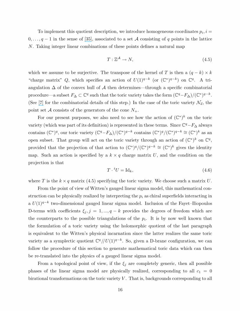
To implement this quotient description, we introduce homogeneous coordinates pi, i =

0, . . . , q − 1 in the sense of [35], associated to a set A consisting of q points in the lattice

N . Taking integer linear combinations of these points defines a natural map

T : ZA → N, (4.5)

which we assume to be surjective. The transpose of the kernel of T is then a (q − k) × k

“charge matrix” Q, which specifies an action of U(1)q−k (or (C∗)q−k) on Cq. A tri-

angulation ∆ of the convex hull of A then determines—through a specific combinatorial

procedure—a subset F∆ ⊂ Cq such that the toric variety takes the form (Cq−F∆)/(C∗)q−k.

(See [7] for the combinatorial details of this step.) In the case of the toric variety N~a, the

point set A consists of the generators of the cone N+.

For our present purposes, we also need to see how the action of (C∗)k on the toric

variety (which was part of its definition) is represented in these terms. Since Cq−F∆ always

contains (C∗)q, our toric variety (Cq−F∆)/(C∗)q−k contains (C∗)q/(C∗)q−k ∼= (C∗)k as an

open subset. That group will act on the toric variety through an action of (C∗)k on Cq,

provided that the projection of that action to (C∗)q/(C∗)q−k ∼= (C∗)k gives the identity

map. Such an action is specified by a k × q charge matrix U , and the condition on the

projection is that

T · tU = Idk, (4.6)

where T is the k × q matrix (4.5) specifying the toric variety. We choose such a matrix U .

From the point of view of Witten’s gauged linear sigma model, this mathematical con-

struction can be physically realized by interpreting the pi as chiral superfields interacting in

a U(1)q−k two-dimensional gauged linear sigma model. Inclusion of the Fayet–Iliopoulos

D-terms with coefficients ξj , j = 1, ..., q − k provides the degrees of freedom which are

the counterparts to the possible triangulations of the pi. It is by now well known that

the formulation of a toric variety using the holomorphic quotient of the last paragraph

is equivalent to the Witten’s physical incarnation since the latter realizes the same toric

variety as a symplectic quotient Cq//U(1)q−k. So, given a D-brane configuration, we can

follow the procedure of this section to generate mathematical toric data which can then

be re-translated into the physics of a gauged linear sigma model.

From a topological point of view, if the ξj are completely generic, then all possible

phases of the linear sigma model are physically realized, corresponding to all c1 = 0

birational transformations on the toric variety V . That is, backgrounds corresponding to all

16

possible triangulations of the point set A are realized. If, on the contrary, only a restricted

set of values for the ξj are physical, then only a subset of the possible phases will be probed.

This is precisely what happens in constructing the D-brane moduli space. Namely, as we

shall see below in the context of two examples, the D-brane vacuum moduli space on

C3/Zn gives precisely the standard toric point set A for the blow-up of C3/Zn. However,

the ξi parameters, determined by the ζj from the last section, are not generic and therefore

only part of the phase space of the blown-up orbifold is probed by D-branes. Although

we do not have a general proof, in the examples we have studied (and in examples studied

by Sardo Infirri [6]) the phases which are eliminated are non-geometric phases reviewed

earlier. This dovetails nicely with the result of Witten in [14] in which he found that the

non-geometric phases are the ones which get squeezed out when passing to strongly coupled

type IIA string theory—that is, M-theory. It is in this limit that D0-branes dominate low

energy physics, and hence the fact that their vacuum moduli space—which we interpret as

an effective spacetime background—does not see the non-geometric phases is in agreement

with Witten’s result.

To see this explicitly, we follow the procedure outlined above. Namely, we express the

solution to the superpotential constraint in terms of a cone M+. We take its dual to get

a cone N+. The q generators of N+ determine a map T : ZA → N , and the transpose

of the kernel of T determines a (q − n − 2) × q charge matrix Q. In order to obtain N~a

as the symplectic quotient Cq //U(1)q−n−2, we must set the associated D-terms ξ1, . . . ,

ξq−n−2 to zero. To describe the action of the U(1)n−1 charges in the twisted sectors on

N~a, we represent the action of U(1)n−1 on Cn+2 by an (n − 1) × (n + 2) charge matrix

V ; the product V U will then give an (n − 1) × q charge matrix for the action of U(1)n−1

on Cq. (This charge matrix depends on the choice of a matrix U satisfying (4.6), but

different choices will only differ by charges from the matrix Q.) Non-zero values of the

corresponding D-terms ξi = ζi−(q−n−2) are allowed.

The full set of charges is now given by a (q−3)×q charge matrix Q, the concatenation

of Q and V U . The cokernel of its transpose gives toric data for the D-brane vacuum moduli

space, in the form of a map T : ZA → Z3. We claim that this data is nothing but the usual

toric data for resolving the quotient space C3/Zn (supplemented by some extra auxiliary

fields as well as some extra U(1)’s which can be used to eliminate them) showing an explicit

realization of the D-brane moduli space aligning with the underlying spacetime structure.

Second, we also claim that the non-genericity of the Fayet–Iliopoulos parameters is such

that the non-geometric phases of this desingularization are not physically realized.

17

We start with the case n = 3. Following the procedure outlined, the cone M+ is

generated by the rows in the following:

x0 y0 z0 z1 z2

x0 1 0 0 0 0x1 1 0 −1 1 0x2 1 0 −1 0 1y0 0 1 0 0 0y1 0 1 −1 1 0y2 0 1 −1 0 1z0 0 0 1 0 0z1 0 0 0 1 0z2 0 0 0 0 1,

(4.7)

and the charges of the fields (x0, y0, z0, . . . , z2) under the twisted sector gauge group U(1)2

(with D-terms ζ1, ζ2, as in (3.4)) are given by

V =

(0 0 0 −1 11 1 1 0 −1

). (4.8)

The dual cone N+ is generated by the columns of

T =

1 0 0 1 0 00 1 0 1 0 00 0 1 1 0 00 0 1 0 1 00 0 1 0 0 1

(4.9)

(which correspond to homogeneous coordinates p0, . . . , p5). The columns of T were found

as solutions of the equations (4.4), with the monomial corresponding to the hyperplane ~n

being∏

X~n·~mi

i .

The transpose of the kernel of this matrix is

Q = ( 1 1 1 −1 −1 −1 ) . (4.10)

We choose U satisfying (4.6) to be

U =

0 −1 −1 1 1 10 1 0 0 0 00 0 1 0 −1 −10 0 0 0 1 00 0 0 0 0 1

, (4.11)

18

so that the full charge matrix Q obtained by concatenating Q and V U is

Q =

1 1 1 −1 −1 −10 0 0 0 −1 10 0 0 1 0 −1

. (4.12)

The cokernel of the transpose of Q (which can be calculated as the transpose of the

kernel) is the matrix

−1 1 0 0 0 0−1 0 1 0 0 03 0 0 1 1 1

. (4.13)

This matrix has three identical columns, which means that the point set A determined by

those columns actually only contains four distinct elements. If we eliminate the redundant

variables and U(1)’s, we obtain a smaller matrix

T =

−1 1 0 0−1 0 1 03 0 0 1

(4.14)

specifying the toric data for the D-brane moduli space N~a//U(1)n−1.

We recognize this as the toric data for resolving C3/Z3. (The charge matrix deter-

mined by T is (1 1 1 −3).) Triangulating on all points yields the blow-up O(−3) → P2.

Leaving out the central point, in the context of type II string theory, would take us to

the Landau–Ginsburg phase, which is geometrically associated with the blown-down sin-

gular variety. In Witten’s gauged linear sigma model, these phases arise from studying the

bosonic potential

U = (|u1|2 + |u2|2 + |u3|2 − 3|p|2 − ξ)2 (4.15)

for ξ positive and for ξ negative. In the former case, vanishing of the potential is consistent

with p = 0, which directly gives the exceptional divisor, P2 with size controlled by ξ. When

ξ is negative, though, p cannot vanish, corresponding to the exceptional divisor being blown

down.

In our case, we have precisely the same toric point set (the columns of (4.14)) but the

Fayet–Iliopoulos parameters ζi are only associated with the last two U(1) quotients in (4.12)

since the first actually originates from a superpotential constraint in the original D-brane

action. As ζ1 and ζ2 take on generic values, it is not hard to see that the corresponding

value of ξ is non-negative, thereby only accessing the blown-up phase. To see this note that

for any non-zero values of the ζi, the second two D-terms imply that two out of the last

19

three homogeneous variables p3, p4, p5 are nonzero. Calling the one that can potentially

vanish p, we can solve the latter two D-term constraints in terms of p and therefore rewrite

the first D-term as

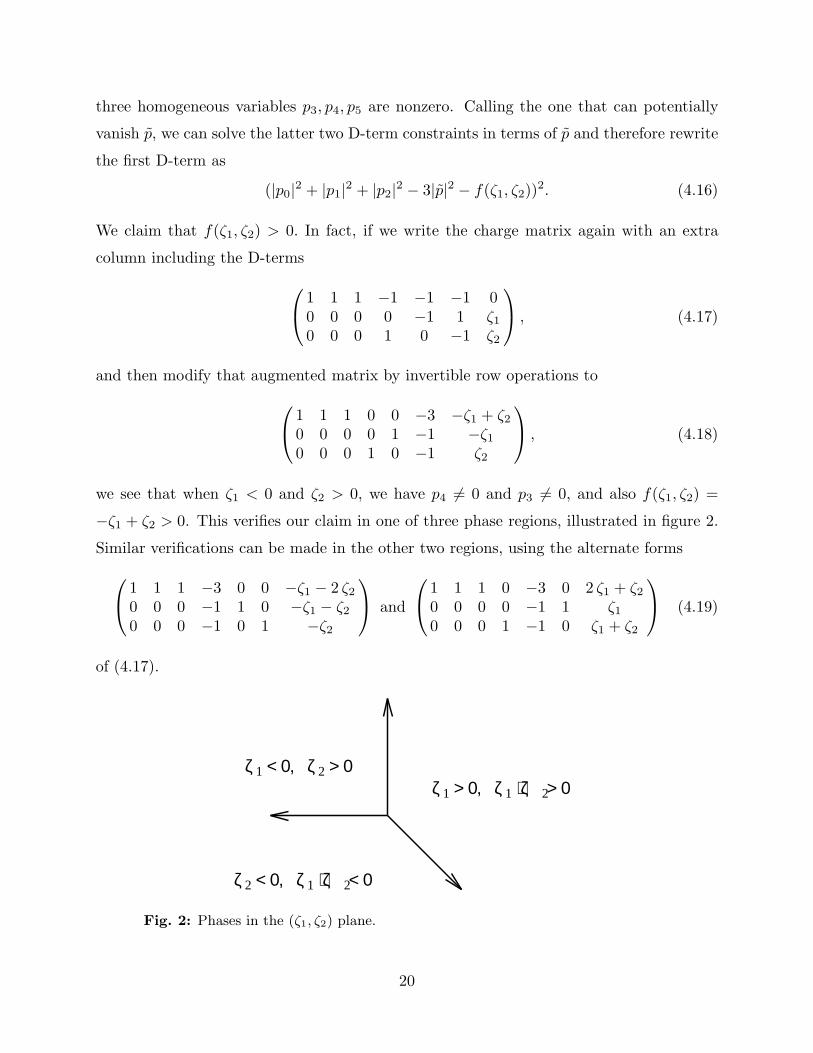
(|p0|2 + |p1|2 + |p2|2 − 3|p|2 − f(ζ1, ζ2))2. (4.16)

We claim that f(ζ1, ζ2) > 0. In fact, if we write the charge matrix again with an extra

column including the D-terms

1 1 1 −1 −1 −1 00 0 0 0 −1 1 ζ1

0 0 0 1 0 −1 ζ2

, (4.17)

and then modify that augmented matrix by invertible row operations to

1 1 1 0 0 −3 −ζ1 + ζ2

0 0 0 0 1 −1 −ζ1

0 0 0 1 0 −1 ζ2

, (4.18)

we see that when ζ1 < 0 and ζ2 > 0, we have p4 6= 0 and p3 6= 0, and also f(ζ1, ζ2) =

−ζ1 + ζ2 > 0. This verifies our claim in one of three phase regions, illustrated in figure 2.

Similar verifications can be made in the other two regions, using the alternate forms

1 1 1 −3 0 0 −ζ1 − 2 ζ2

0 0 0 −1 1 0 −ζ1 − ζ2

0 0 0 −1 0 1 −ζ2

and

1 1 1 0 −3 0 2 ζ1 + ζ2

0 0 0 0 −1 1 ζ1

0 0 0 1 −1 0 ζ1 + ζ2

(4.19)

of (4.17).

1 ζ + ζ > 021ζ > 0,

212ζ < 0, ζ + ζ < 0

1 ζ > 0ζ < 0, 2

Fig. 2: Phases in the (ζ1, ζ2) plane.

20

The case of n = 5 is similar, but technically more involved. Taking the action to be

(Z1, Z2, Z3) → (ω3Z1, ω3Z2, ω−1Z3), we find that the cone M+ is generated by the rows

in the following:

x0 y0 z0 z1 z2 z3 z4

x0 1 0 0 0 0 0 0x1 1 0 0 1 0 0 −1x2 1 0 −1 1 1 0 −1x3 1 0 −1 0 1 1 −1x4 1 0 −1 0 0 1 0y0 0 1 0 0 0 0 0y1 0 1 0 1 0 0 −1y2 0 1 −1 1 1 0 −1y3 0 1 −1 0 1 1 −1y4 0 1 −1 0 0 1 0z0 0 0 1 0 0 0 0z1 0 0 0 1 0 0 0z2 0 0 0 0 1 0 0z3 0 0 0 0 0 1 0z4 0 0 0 0 0 0 1,

(4.20)

and the charges of the fields (x0, y0, z0, . . . , z4) under the twisted sector gauge group U(1)4

(with D-terms ζ1, . . . , ζ4, as in (3.4)) are given by

V =

0 0 0 −1 1 0 00 0 0 0 −1 1 01 1 0 0 0 −1 10 0 1 0 0 0 −1

. (4.21)

The dual cone N+ is generated by the columns of

T =

1 0 0 1 0 0 0 0 1 0 0 0 10 1 0 1 0 0 0 0 1 0 0 0 10 0 1 1 0 0 1 1 1 0 0 0 00 0 1 0 1 1 1 0 0 1 0 0 00 0 1 1 1 0 0 1 0 0 1 0 00 0 1 0 0 1 1 1 0 0 0 1 00 0 1 1 1 1 0 0 0 0 0 0 1

(4.22)

(which correspond to homogeneous coordinates p0, . . . , p12). We choose U satisfying (4.6)

to be

U =

1 0 0 0 0 0 0 0 0 0 0 0 00 1 0 0 0 0 0 0 0 0 0 0 0−1 −1 0 0 0 0 0 0 1 0 0 0 00 0 0 0 0 0 0 0 0 1 0 0 00 0 0 0 0 0 0 0 0 0 1 0 00 0 0 0 0 0 0 0 0 0 0 1 0−1 −1 0 0 0 0 0 0 0 0 0 0 1

, (4.23)

21

so that the full charge matrix Q obtained by concatenating Q = t(ker T ) and V U (and

including an extra column for the D-terms) is

Q =

1 1 0 2 −1 −1 2 −1 −3 0 0 0 0 00 0 1 −1 0 0 −1 0 1 0 0 0 0 00 0 0 0 0 0 −1 1 0 1 −1 0 0 00 0 0 0 −1 1 0 0 0 0 1 −1 0 00 0 0 1 0 0 0 −1 0 0 0 1 −1 00 0 0 0 0 −1 1 0 −1 0 0 0 1 00 0 0 0 0 0 0 0 0 −1 1 0 0 ζ1

0 0 0 0 0 0 0 0 0 0 −1 1 0 ζ2

0 0 0 0 0 0 0 0 0 0 0 −1 1 ζ3

0 0 0 0 0 0 0 0 1 0 0 0 −1 ζ4

. (4.24)

The cokernel of the transpose of Q (which can be calculated as the transpose of the

kernel) is the matrix

−1 1 0 0 0 0 0 0 0 0 0 0 0−3 0 1 0 0 0 0 0 −1 −1 −1 −1 −15 0 0 1 1 1 1 1 2 2 2 2 2

. (4.25)

This matrix has two sets of identical columns (with five in each set), which means that

the point set A determined by the columns actually only contains five distinct elements.

If we eliminate the redundant variables and U(1)’s, we obtain a smaller matrix

T =

−1 1 0 0 0−3 0 1 0 −15 0 0 1 2

(4.26)

specifying the toric data for the D-brane moduli space N~a//U(1)n−1. The corresponding

charge matrix t(ker T ) is (1 1 0 1 −30 0 1 −2 1

). (4.27)

We recognize this toric data in R3 as that for C

3/Z5. From the point of view of a

symplectic quotient or the gauged linear sigma model, this corresponds to five chiral fields

with bosonic potential

U = (|u1|2 + |u2|2 + |u4|2 − 3|p|2 − ξ1)2 + (|u3|2 − 2|u4|2 + |p|2 − ξ2)

2. (4.28)

This linear sigma model has four phases, one of which is the (single) smooth geometrical

resolution (represented by ξ1 > 0, ξ2 > 0), two of which are orbifold phases (in which

22

one or other of the exceptional divisors has been blown-down) and a Landau–Ginsburg

phase (where this terminology is more apt for models with a superpotential, but we retain

the common labeling scheme). As before, if we had completely generic Fayet–Iliopoulos

terms associated with each row of the full U(1)10 charge matrix (4.24), then the D-brane

moduli space would probe all four of these phases. But, since we only have non-zero ζj

associated with the U(1)4 twisted sector gauge group, this is not the case. Rather, the

three “non-geometrical” phases which disappear in the strongly coupled type IIA string

are not realized as the ζ’s take on all possible values: only the geometric phase is probed

by the D-branes.

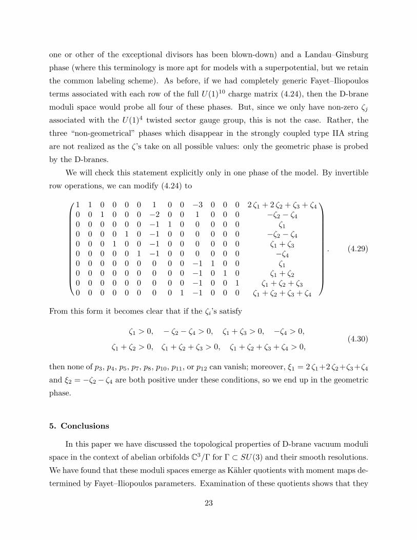
We will check this statement explicitly only in one phase of the model. By invertible

row operations, we can modify (4.24) to

1 1 0 0 0 0 1 0 0 −3 0 0 0 2 ζ1 + 2 ζ2 + ζ3 + ζ4

0 0 1 0 0 0 −2 0 0 1 0 0 0 −ζ2 − ζ4

0 0 0 0 0 0 −1 1 0 0 0 0 0 ζ1

0 0 0 0 1 0 −1 0 0 0 0 0 0 −ζ2 − ζ4

0 0 0 1 0 0 −1 0 0 0 0 0 0 ζ1 + ζ3

0 0 0 0 0 1 −1 0 0 0 0 0 0 −ζ4

0 0 0 0 0 0 0 0 0 −1 1 0 0 ζ1

0 0 0 0 0 0 0 0 0 −1 0 1 0 ζ1 + ζ2

0 0 0 0 0 0 0 0 0 −1 0 0 1 ζ1 + ζ2 + ζ3

0 0 0 0 0 0 0 0 1 −1 0 0 0 ζ1 + ζ2 + ζ3 + ζ4

. (4.29)

From this form it becomes clear that if the ζi’s satisfy

ζ1 > 0, − ζ2 − ζ4 > 0, ζ1 + ζ3 > 0, −ζ4 > 0,

ζ1 + ζ2 > 0, ζ1 + ζ2 + ζ3 > 0, ζ1 + ζ2 + ζ3 + ζ4 > 0,(4.30)

then none of p3, p4, p5, p7, p8, p10, p11, or p12 can vanish; moreover, ξ1 = 2 ζ1+2 ζ2+ζ3+ζ4

and ξ2 = −ζ2 − ζ4 are both positive under these conditions, so we end up in the geometric

phase.

5. Conclusions

In this paper we have discussed the topological properties of D-brane vacuum moduli

space in the context of abelian orbifolds C3/Γ for Γ ⊂ SU(3) and their smooth resolutions.

We have found that these moduli spaces emerge as Kahler quotients with moment maps de-

termined by Fayet–Iliopoulos parameters. Examination of these quotients shows that they

23

are birational to the singular space C3/Γ with the Fayet–Iliopoulos parameters controlling

the size of the blow-up to a smooth space. This alignment of the vacuum moduli space

and the ambient background space provides another strong piece of evidence that spatial

backgrounds at ultrashort distances can be thought of as a derivative concept emerging

from the fundamental notion of a vacuum moduli space.

The classical vacuum moduli space coincides with the moduli space of another theory,

a gauged linear sigma model with no superpotential, motivated by considerations of toric

geometry.4 Hence, the moduli space can a priori have a rich phase structure. However,

non-genericity of the Fayet–Iliopoulos parameters appears to ensure that the non-geometric

phases are not part of the physical vacuum D-brane moduli space.

The neighborhood of an orbifold point can contain other transitions. For example, the

C3/Z11 orbifold has multiple resolutions, connected by flops. This D-brane linear sigma

model will contain an explicit geometric realization of the flop, and it will be interesting

to work this out.

It is worth noting that even for Γ 6⊂ SU(3), the D-brane theory defined as a quotient

of N = 4 super-Yang–Mills theory is a sensible non-supersymmetric gauge theory, whose

classical moduli space (on the Higgs branch) is an ALE space asymptotic to C3/Γ, also

studied in [5,6]. These are non-supersymmetric theories with special matter content, and

it would be interesting to see if this moduli space survives in the quantum theory.

Acknowledgments

We thank the members of the Rutgers high energy theory group for discussions; B.R.G.

and D.R.M. also thank the Rutgers group for hospitality during various stages of this

project. The work of M.R.D. is supported by DOE grant DE-FG02-96ER40959. The

work of B.R.G. is supported by a National Young Investigator Award and the Alfred P.

Sloan Foundation. The work of D.R.M. is supported in part by the Harmon Duncombe

Foundation and by NSF grants DMS-9401447 and DMS-9627351.

4 It would be interesting to relate the D-brane worldvolume theory to this other theory more

directly, perhaps by means of a duality transformation in which the massive states associated to

“fractional branes” play a role.

24

References

[1] M. R. Douglas and G. Moore, “D-Branes, Quivers, and ALE Instantons,” hep-

th/9603167.

[2] J. Polchinski, “Tensors from K3 Orientifolds,” hep-th/9606165.

[3] C. Johnson and R. Myers, “Aspects of Type IIB Theory on ALE Spaces,” hep-

th/9610140.

[4] P. B. Kronheimer, “The Construction of ALE Spaces as Hyper-Kahler Quotients,” J.

Diff. Geom. 29 (1989) 665.

[5] A. V. Sardo Infirri, “Partial Resolutions of Orbifold Singularities via Moduli Spaces

of HYM-type Bundles,” alg-geom/9610004.

[6] A. V. Sardo Infirri, “Resolutions of Orbifold Singularities and Flows on the McKay

Quiver,” alg-geom/9610005.

[7] P. S. Aspinwall, B. R. Greene and D. R. Morrison, “Calabi–Yau Moduli Space, Mirror

Manifolds and Spacetime Topology Change in String Theory,” Nucl. Phys. B416 (1994)

414; hep-th/9309097.

[8] E. Witten, “Phases of N=2 Theories In Two Dimensions,” Nucl. Phys. B403 (1993)

159; hep-th/9301042.

[9] P. S. Aspinwall, B. R. Greene and D. R. Morrison, “Measuring Small Distances in

N=2 Sigma Models,” Nucl. Phys. B420 (1994) 184; hep-th/9311042.

[10] T. Banks, W. Fischler, S. H. Shenker and L. Susskind, “M Theory as a Matrix Model:

A Conjecture,” hep-th/9610043.

[11] M. R. Douglas, “Enhanced Gauge Symmetry in M(atrix) Theory,” hep-th/9612126.

[12] M. R. Douglas, H. Ooguri and S. H. Shenker, “Issues in M(atrix) Theory Compacti-

fication,” hep-th/9702203.

[13] M. R. Douglas and B. R. Greene, to appear.

[14] E. Witten, “Phase Transitions In M-Theory And F-Theory,” Nucl. Phys. B471 (1996)

195; hep-th/9603150.

[15] P. S. Aspinwall and B. R. Greene, “On the Geometric Interpretation of N=2 Super-

conformal Theories,” Nucl. Phys. B437 (1995) 205; hep-th/9409110.

[16] D. R. Morrison and M. R. Plesser, “Summing the Instantons: Quantum Cohomol-

ogy and Mirror Symmetry in Toric Varieties,” Nucl. Phys. B440 (1995) 279; hep-

th/9412236.

[17] P. S. Aspinwall, “Enhanced Gauge Symmetries and K3 Surfaces,” Phys. Lett. B357

(1995) 329; hep-th/9507012.

[18] O. J. Ganor, D. R. Morrison, and N. Seiberg, “Branes, Calabi–Yau Spaces, and

Toroidal Compactification of the N=1 Six-Dimensional E8 Theory,” Nucl. Phys. B487

(1997) 93; hep-th/9610251.

[19] D. R. Morrison and M. R. Plesser, to appear.

25

[20] L. Dixon, J. A. Harvey, C. Vafa, and E. Witten, “Strings on Orbifolds, I, II” Nucl.

Phys. B261 (1985) 678; Nucl. Phys. B274 (1986) 285.

[21] J. Polchinski and Y. Cai, “Consistency of Open Superstring Theories,” Nucl. Phys.

B296 (1988) 91.

[22] M. R. Douglas, “Branes within Branes,” hep-th/9512077.

[23] H. Ooguri, Y. Oz and Z. Yin, “D-Branes on Calabi–Yau Spaces and Their Mirrors,”

Nucl.Phys. B477 (1996) 407; hep-th/9606112.

[24] E. G. Gimon and J. Polchinski, “Consistency Conditions for Orientifolds and D-

Manifolds,” Phys. Rev. D54 (1996) 1667; hep-th/9601038.

[25] A. Sagnotti, “Some Properties of Open-String Theories,” hep-th/9509080.

[26] Y. Ito and M. Reid, “The McKay Correspondence for Finite Subgroups of SL(3,C),”

in: Higher Dimensional Complex Varieties (M. Andreatta et al., eds.), de Gruyter,

1996, p. 221; alg-geom/9411010.

[27] M. Reid, “McKay Correspondence,” alg-geom/9702016.

[28] B. R. Greene and Y. Kanter, “Small Volumes in Compactified String Theory,” hep-

th/9612181.

[29] T. Banks, N. Seiberg, and E. Silverstein, “Zero and One-dimensional Probes with

N=8 Supersymmetry,” hep-th/9703052.

[30] M. R. Douglas, to appear.

[31] T. Oda, Convex Bodies and Algebraic Geometry, Springer-Verlag, 1988.

[32] W. Fulton, Introduction to Toric Varieties, Princeton University Press, 1993.

[33] T. Delzant, “Hamiltoniens periodiques et images convexe de l’application moment,”

Bull. Soc. Math. France 116 (1988) 315.

[34] M. Audin, The Topology of Torus Actions on Symplectic Manifolds, Birkhauser, 1991.

[35] D. A. Cox, “The Homogeneous Coordinate Ring of a Toric Variety,” J. Algebraic

Geom. 4 (1995) 17; alg-geom/9210008.

26