arX

iv:0

901.

3905

v1 [

hep-

th]

26

Jan

2009

TCDMATH 09-03

Strong Homotopy Lie Algebras, Generalized

Nahm Equations and Multiple M2-branes

Calin Iuliu-Lazaroiu, Daniel McNamee, Christian Samann and Aleksandar Zejak

Hamilton Mathematics Institute and

School of Mathematics,

Trinity College, Dublin 2, Ireland

E-mail: calin, danmc, saemann, zejak@maths.tcd.ie

Abstract

We review various generalizations of the notion of Lie algebras, in particular

those appearing in the recently proposed Bagger-Lambert-Gustavsson model, and

study their interrelations. We find that Filippov’s n-Lie algebras are a special

case of strong homotopy Lie algebras. Furthermore, we define a class of homotopy

Maurer-Cartan equations, which contains both the Nahm and the Basu-Harvey

equations as special cases. Finally, we show how the super Yang-Mills equations

describing a Dp-brane and the Bagger-Lambert-Gustavsson equations supposedly

describing M2-branes can be rewritten as homotopy Maurer-Cartan equations, as

well.

1. Introduction and results

Since Witten’s introduction of M-theory, our understanding of this proposal for a non-

perturbative unification of the various superstring models has grown quite slowly. Little

more than a year ago, however, a description of the effective dynamics of stacks of M2-

branes was proposed by Bagger, Lambert and independently by Gustavsson [1, 2]. The

construction of the Bagger-Lambert-Gustavsson (BLG) model relies crucially on mathemat-

ical structures known as 3-Lie algebras [3]. It was soon found that the BLG model together

with the special 3-Lie algebra A4 should be interpreted as the effective description of a stack

of two M2-branes [4]. Unfortunately, subsequent analysis showed that this is the only 3-Lie

algebra which can be used in the construction of the BLG theory [5]; all other 3-Lie algebras

suitable for that purpose are direct sums of A4.

Therefore, a generalization of the BLG model is clearly needed and over the last year,

three such generalizations were pursued. First, positive definiteness of the bilinear pairing of

the 3-Lie algebra was relaxed. This leads to ghosts in the theory, which have to be removed.

At least one of these procedures [6] yields d = 3, N = 8 super Yang-Mills (SYM) theory, which

is not the desired outcome. Second, it was noticed that the BLG model can be rewritten as

a gauge theory [7] having a Lie algebra as its gauge algebra. Thus, the original incarnation

of the BLG model in terms of 3-Lie algebras might have been misleading and 3-Lie algebras

could have entered the theory only accidentally for the case of two M2-branes. Third, one can

use an extended version of 3-Lie algebras, which in general leads to theories with a smaller

amount of supersymmetry than the original N = 8 of the BLG model [8, 9, 10, 11].

In this note, we present evidence that the BLG model based on 3-Lie algebras should

be reconsidered within the framework of strong homotopy Lie algebras, also known as L∞algebras [12, 13]. These are natural generalizations of Lie algebras arising in algebraic homo-

topy theory and deformation theory. Just as one can consider the Maurer-Cartan equation

describing deformation problems governed by a Lie algebra, an L∞ algebra defines a ‘ho-

motopy Maurer-Cartan (hMC) equation’ related to an associated deformation problem [14].

In a physics context, L∞ algebras and homotopy Maurer-Cartan equations have appeared

naturally in string field theory [15], BV quantization [16], topological open string theory and

topological field theory [17, 18, 19, 20, 21, 22, 23] as well as gauge theory [24].

Certain classical field equations can be written in the form of homotopy Maurer-Cartan

equations associated with appropriate L∞ algebras. For example, Yang-Mills theory and its

maximally supersymmetric extension were discussed in [25] and [26], the Einstein equations

were rewritten in hMC form up to second order in [27]. All this, together with the results of

this paper, supports the conjecture of Andrei S. Losev that for all classical field equations,

an interpretation in terms of hMC equations exists.

As a side remark, we note that the twistor description provides an alternate route to

reformulating field equations in hMC form. Over twistor space, solutions to classical field

equations correspond to topologically trivial holomorphic vector bundles over a twistor space

P. Such vector bundles can be described in terms of holomorphic connections given locally

by gauge potentials A0,1 ∈ Ω0,1(P, g) which are holomorphically flat, i.e. they satisfy the

Maurer Cartan equation

F0,2 := ∂A0,1 + A0,1 ∧A0,1 = 0 . (1.1)

1

Here, g is an ordinary Lie algebra, and thus the twistor description yields an equivalence

between classical field equations and Maurer-Cartan equations for connection one-forms tak-

ing values in a Lie algebra. For more details and examples of field theories allowing for

a twistorial description, see e.g. [28] and references therein. This approach, however, re-

quires an auxiliary twistor space, while the above mentioned reformulations of Yang-Mills

and Einstein equations in terms of hMC equations live on the same space as the original

equations.

In this paper, we place the BLG model into the context of L∞ algebras and hMC equa-

tions. First, we review the relations between Filippov’s n-Lie algebras, Lie n-algebras and

L∞ algebras. We find that n-Lie algebras are a special class of ungraded L∞ algebras. We

then construct a family of models given by hMC equations and special L∞ algebras, which

correspond to Nahm-type equations. In particular, both the Nahm and the Basu-Harvey

equations [29] are contained in this family as special cases. After this, we discuss L∞ alge-

bras whose hMC equations yield both the SYM equations1 as well as the full supersymmetric

BLG equations. We conclude with a few remarks on the reduction process from the BLG

equations to the SYM equations.

2. Higher Lie structures

We shall need certain successive generalizations of the notion of a Lie algebra, all of which

are based on promoting the Lie bracket to operations of higher arity, and on successive

weakenings of the classical Jacobi identity. There are two types of generalizations, which can

be classified into graded and ungraded, depending on whether the underlying vector space

and operations are required or not to be graded or homogeneous2. The mathematical details

can be found in the Appendix.

2.1. Ungraded generalizations of the notion of a Lie algebra

The first ungraded generalization useful for our purpose is provided by the notion of a n-Lie

algebra, which was introduced by Filippov [3]. To define such algebras, one replaces the Lie

bracket by an n-ary operation which is required to be totally antisymmetric and to obey a

partial weakening of the Jacobi identity known as Filippov’s fundamental identity.

A wider generalization is provided by the notion of Lie n-algebra in the sense of Hanlon

and Wachs [30], which again uses a single totally antisymmetric n-operation of higher arity,

this time required to obey a further weakening of the Jacobi identity which we shall call

the homotopy Jacobi identity. It was shown in [31] that n-Lie algebras are Lie n-algebras,

because Filippov’s fundamental identity implies the homotopy Jacobi identity.

The widest generalization we shall need is the notion of a (ungraded) strong homotopy

Lie (or L∞) algebra, which is well-known in algebraic homotopy theory, where it originated.

This is obtained by allowing for a countable family of multilinear antisymmetric operations

1Our rewriting of this theory differs from that found in [26].2More generally, each higher Lie structure can be defined as an algebra object in a certain monoidal

category V. The ungraded extensions arise by taking V to be the category of vector spaces over some field k

of characteristic zero, while the graded extensions arise when V is a category of graded vector spaces over k.

2

of all arities n ≥ 1, constrained by a countable series of generalizations of the Jacobi identity

known as the L∞ identities. This notion admits specializations indexed by subsets3 S ⊂ N∗

of arities and which are defined by requiring vanishing of all products of arities not belonging

to S. This leads to the notion of LS algebra. When S = n1, . . . , np is a finite set (with

n1 < . . . < np), the result of this specialization is called an Ln1,...,np algebra, also known as

an L(N) algebra when S = 1, . . . , N. The case S = n, when only a single product of

arity n is non-vanishing, recovers the notion of a Lie n-algebra, i.e. all n-Lie algebras are Ln

algebras. All in all, we have a series of successive generalizations:

Lie algebras ⊂ n-Lie algebras ⊂ Lie n-algebras

q

Ln algebras ⊂ (ungraded) L∞ algebras

We refer the reader to the Appendix for more details.

2.2. Graded versions

An obvious variant of the algebraic structures above is to consider their graded versions. In

this case the underlying vector space is graded, and each operation is graded-antisymmetric

as well as homogeneous of a certain degree. The various extensions of the Jacobi identity

are replaced by graded variants, which now contain appropriate sign factors. In general, one

can consider a grading through elements of an Abelian group G, and define the signs appear-

ing in various equations (such as the graded antisymmetry and graded Filippov/homotopy

Jacobi/L∞ identities) by using a group morphism φ from G to Z2. This leads to the notions

of (G,φ)-graded n-Lie algebras, Lie n-algebras and L∞ algebras/LS algebras:

graded Lie algebras ⊂ graded n-Lie algebras ⊂ graded Lie n-algebras

q

graded Ln algebras ⊂ graded L∞ algebras

The choice G = 0 (the trivial Abelian group) and φ = 0 recovers the ungraded theo-

ries, whose multilinear operations are antisymmetric in the usual sense rather than graded

antisymmetric. In the L∞ case, the choices G = Z, φ(n) = n(mod 2) and G = Z2, φ = idZ2

recover the notions of Z- and Z2-graded L∞ algebras as they appear in algebraic homotopy

theory. More details can be found in the Appendix.

Remark. For other generalizations of 3-Lie algebras appearing in the Bagger-Lambert

model as well as their relations to Lie triple systems, see [8, 9, 10]. There, however, the

multilinear operations are not totally antisymmetric. As noted in the conclusions of [11],

they might find an interpretation within a further extension of Lie algebras, the strong

homotopy pre-Lie algebras.

3Here N∗ = 1, 2, 3, . . . is the set of non-vanishing natural numbers.

3

2.3. Homotopy Maurer-Cartan equations

Given a Z-graded L∞ algebra L (see Appendix), the homotopy Maurer-Cartan equations

(hMC) are the following equations for an element φ of L which is weakly-homogeneous of

odd parity:∑

ℓ≥1

(−1)ℓ(ℓ+1)/2

ℓ!µℓ(φ, . . . , φ) = 0 . (2.1)

Here µℓ are the multiplications in L. These equations are invariant under the infinitesimal

gauge transformations:

δφ = −∑

ℓ≥1

(−1)ℓ(ℓ−1)/2

(ℓ− 1)!µℓ(λ, φ, . . . , φ) , (2.2)

where λ is a a weakly-homogeneous element of L of even parity, playing the role of a gauge

generator. We illustrate this in some two particular cases:

(1) In a differential Z-graded Lie algebra with µ1 = d and µ2 = [ , ], the hMC equations

reduce to the classical Maurer-Cartan equations:

dφ+1

2[φ, φ] = 0 . (2.3)

(2) In an L1,2,n algebra with µ1 = d and µ2(a, b) = [a, b], they take the form:

dφ+1

2[φ, φ] +

(−1)n(n+1)/2

n!µn(φ, . . . , φ) = 0 . (2.4)

3. A unifying framework for Nahm-type equations

3.1. A family of L∞ algebras

Let V be an (n + 1)-dimensional complex vector space endowed with a nondegenerate C-

bilinear symmetric form ( , ). Below, we consider the Clifford algebra C(V,Q), where Q is

the quadratic form defined by ( , ); if there is a canonical choice for Q, we also write C(V )

as a shorthand. Picking an orthonormal basis e1 . . . en+1 of V , this can be presented as the

unital associative algebra generated by ei with the relations:

eiej + ejei = 2δij (3.1)

Let Am : V ×r → C(V,Q) be the antisymmetrization operator:

Am(v1, . . . , vm) :=1

m!

∑

σ∈Sm

ǫ(σ)vσ(1) . . . vσ(m) , (3.2)

where juxtaposition in the right hand side stands for the multiplication in C(V,Q). Since

each map Am is multilinear and alternating, it factors through a map Am : ∧mV → C(V,Q).

Setting ∧•V := ⊕n+1m=0 ∧m V , it is well-known that the map A :=

∑n+1m=0 Am : ∧•V → C(V,Q)

is a linear isomorphism. We will use the standard notation e[i1 . . . eim] for the element

Am(ei1 , . . . , eim) of C(V,Q). Via the isomorphism A, the grading on ∧•V induces a grad-

ing of the underlying vector space of C(V,Q), whose homogeneous subspaces we denote by

4

Cm(V,Q); these subspaces of the Clifford algebra are isomorphic with ∧mV via the maps

Am. Of course, this grading of C(V,Q) is not preserved by the Clifford multiplication.

Consider the element e := e1...en+1 of Cn+1(V,Q), which corresponds to the non-vanishing

element e1 ∧ . . .∧ en+1 of the determinant line ∧n+1V via the isomorphism An+1 : ∧n+1V →Cn+1(V,Q). From (3.1), we have the following identities:

e2 = 1 and eei1 ...ein = n!ǫii1...inei . (3.3)

Now let (L, [ , . . . , ]) be an ungraded n-Lie algebra over the complex numbers. If n > 2,

then we consider the vector space:

FL = gL ⊕ L (3.4)

where (gL, [[ , ]]) is the basic Lie algebra of L, whose natural action on L we denote by the

symbol ⊲ (see Appendix). If n = 2, we set FL = L. An element a of ΛiL will be said to

be of order i and we introduce the notation a = i. To describe both the Nahm and the

Basu-Harvey equations themselves, L is sufficient; however, it turns out that including the

other powers allows us to also describe gauge transformations.

Consider the infinite-dimensional complex vector space L := L0 ⊕ L1 ⊕ L2 where L0 :=

Ω0(R) ⊗C gL, L1 := Ω1(R) ⊗C gL ⊕ Ω0(R) ⊗C V ⊗C L and L2 := Ω1(R) ⊗C V ⊗C L. We

view L as a Z-graded vector space whose grading is concentrated in degrees 0, 1 and 2. Also,

we endow L with its natural differential4 µ1(ω) := −(d ⊗ id)ω, where d is the de Rham

differential on the real line R and ω ∈ Ω(R,L). A degree zero element of L is simply a

gL-valued function λ ∈ Ω0(R) ⊗C gL. A degree one element φ of L decomposes as:

φ = X +A (3.5)

where A is a gL-valued one-form on the real line and X is a function on the real line taking

values in the vector space Vn+1 ⊗C L. We view A as a connection one-form for the trivial

principal bundle G over the real line whose fiber is the Lie group obtained by exponentiating

gL, and treat X as a section of the trivial vector bundle over R associated to G via the action

(induced by ⊲) of gL on the vector space Vn+1⊗CL. Accordingly, we let ∇s be the covariant

derivation operator defined by the connection one-form A, i.e dX + A ⊲ X = ∇s(X)ds for

any function X on the real line taking values in Vn+1 ⊗CL. A degree two element ρ of L is a

Vn+1 ⊗C L-valued one-form on the real line. Thus, a general element x ∈ L decomposes as:

x = λ+ φ+ ρ = λ+A+X + ρ . (3.6)

Besides the differential µ1, we introduce the following products on L:

µ2(λ1 +A1 +X1 + ρ1,λ2 +A2 +X2 + ρ2)

:= [[λ1, λ2]] − 2[[λ1, A2]] + 2[[λ2, A1]] − 2λ1 ⊲ X2 + 2λ2 ⊲ X1

− 2A1 ⊲ X2 − 2A2 ⊲ X1 + λ1 ⊲ ρ2 − λ2 ⊲ ρ1

4Here and in the following, we include factors in the products µℓ such that the normalizations in the

equations of motion arising from the hMC equations match the canonical choices.

5

and:

µn(X, ...,X) := − (−1)n(n−1)/2e[X, ...,X]ds = (−1)n(n−1)/2eei1 . . . ein [Xi1 . . . Xin ]ds

= − (−1)n(n−1)/2n!ǫii1...inei[Xi1 . . . Xin ]ds ,

where we decomposed X = Xiei. In fact, the form of these products is fixed by the condition

that the degree of µℓ equals 2− ℓ. This is in particular the reason for the factor ds appearing

in µn. We set µℓ = 0 for all ℓ ∈ Z \ 1, 2, n.It is easy to check that the products introduced above satisfy the homotopy Jacobi iden-

tities (B.37), hence (L, µ1, µ2, µn) is a Z-graded L1,2,n algebra, i.e. a Z-graded L∞ algebra

whose only non-vanishing products are µ1, µ2 and µn (see Appendix). The identity involving

two copies of µn holds because ds∧ ds = 0 on the real line. The other non-trivial homotopy

Jacobi identity involves products µ2(λ, ) and µn(X, . . . ,X), and holds due to relation (A.5),

which in turn is a consequence of Filipov’s fundamental identity (A.2) satisfied by the bracket

of L (see Appendix).

The homotopy Maurer-Cartan equation (2.1) for φ = A+X:

µ1(φ) +1

2µ2(φ, φ) − (−1)n(n+1)/2

n!µn(φ, . . . , φ) = 0 , (3.7)

reduces to:

∇sXi + ǫii1...in [Xi1 , . . . ,Xin ] = 0 , (3.8)

and identity which we shall call the generalized Nahm equation. Since A is flat (we have

dA = 0 for dimension reasons) and R is contractible, the connection A can be gauged away

provided that its behavior at infinity is tame enough.

The infinitesimal gauge transformations (2.2) take the form:

δφ = −µ1(λ) − 12µ2(λ, φ) − (−1)n(n−1)/2

(n− 1)!µn(λ, φ, . . . , φ) . (3.9)

Since the last term vanishes in our case, this is the same as:

δφ = µ1(λ) + µ2(λ, φ) , (3.10)

or, more explicitly:

δA = dλ+ [[λ,A]] , (3.11)

δX = λ ⊲ X ,

where λ ∈ Ω0(R) ⊗ gL as above.

In the following, we discuss the two special cases n = 2 and n = 3, which correspond to

the Nahm and Basu-Harvey equations, respectively.

3.2. The L∞ algebra of the Nahm equation

The Nahm equation was originally introduced to extend the ADHM construction of instan-

tons to the case of monopoles [32, 33]. Later, this construction found an interpretation in

terms of D-branes in superstring theory [34]. In this interpretation, one considers a stack of

6

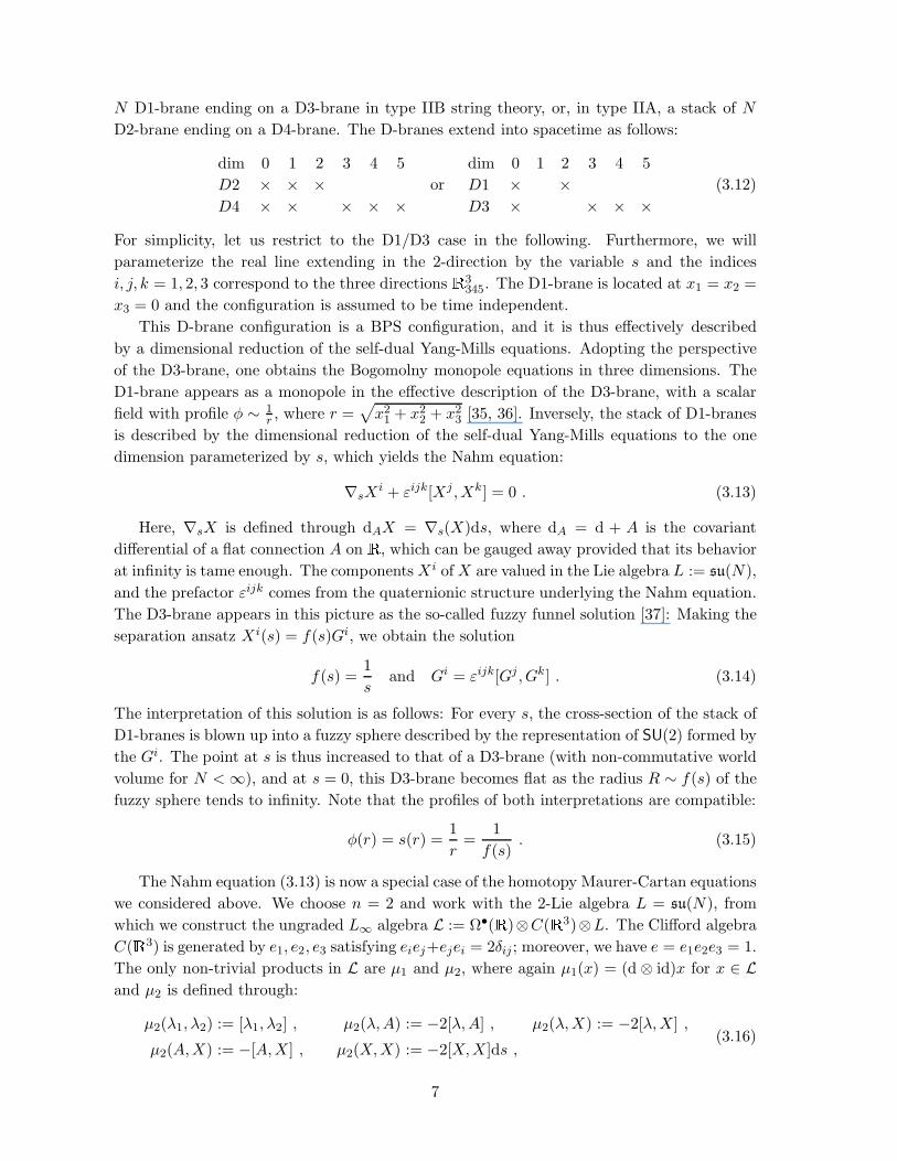
N D1-brane ending on a D3-brane in type IIB string theory, or, in type IIA, a stack of N

D2-brane ending on a D4-brane. The D-branes extend into spacetime as follows:

dim 0 1 2 3 4 5

D2 × × ×D4 × × × × ×

or

dim 0 1 2 3 4 5

D1 × ×D3 × × × ×

(3.12)

For simplicity, let us restrict to the D1/D3 case in the following. Furthermore, we will

parameterize the real line extending in the 2-direction by the variable s and the indices

i, j, k = 1, 2, 3 correspond to the three directions R3345. The D1-brane is located at x1 = x2 =

x3 = 0 and the configuration is assumed to be time independent.

This D-brane configuration is a BPS configuration, and it is thus effectively described

by a dimensional reduction of the self-dual Yang-Mills equations. Adopting the perspective

of the D3-brane, one obtains the Bogomolny monopole equations in three dimensions. The

D1-brane appears as a monopole in the effective description of the D3-brane, with a scalar

field with profile φ ∼ 1r , where r =

√

x21 + x2

2 + x23 [35, 36]. Inversely, the stack of D1-branes

is described by the dimensional reduction of the self-dual Yang-Mills equations to the one

dimension parameterized by s, which yields the Nahm equation:

∇sXi + εijk[Xj ,Xk] = 0 . (3.13)

Here, ∇sX is defined through dAX = ∇s(X)ds, where dA = d + A is the covariant

differential of a flat connection A on R, which can be gauged away provided that its behavior

at infinity is tame enough. The componentsXi ofX are valued in the Lie algebra L := su(N),

and the prefactor εijk comes from the quaternionic structure underlying the Nahm equation.

The D3-brane appears in this picture as the so-called fuzzy funnel solution [37]: Making the

separation ansatz Xi(s) = f(s)Gi, we obtain the solution

f(s) =1

sand Gi = εijk[Gj , Gk] . (3.14)

The interpretation of this solution is as follows: For every s, the cross-section of the stack of

D1-branes is blown up into a fuzzy sphere described by the representation of SU(2) formed by

the Gi. The point at s is thus increased to that of a D3-brane (with non-commutative world

volume for N <∞), and at s = 0, this D3-brane becomes flat as the radius R ∼ f(s) of the

fuzzy sphere tends to infinity. Note that the profiles of both interpretations are compatible:

φ(r) = s(r) =1

r=

1

f(s). (3.15)

The Nahm equation (3.13) is now a special case of the homotopy Maurer-Cartan equations

we considered above. We choose n = 2 and work with the 2-Lie algebra L = su(N), from

which we construct the ungraded L∞ algebra L := Ω•(R)⊗C(R3)⊗L. The Clifford algebra

C(R3) is generated by e1, e2, e3 satisfying eiej+ejei = 2δij ; moreover, we have e = e1e2e3 = 1.

The only non-trivial products in L are µ1 and µ2, where again µ1(x) = (d ⊗ id)x for x ∈ Land µ2 is defined through:

µ2(λ1, λ2) := [λ1, λ2] , µ2(λ,A) := −2[λ,A] , µ2(λ,X) := −2[λ,X] ,

µ2(A,X) := −[A,X] , µ2(X,X) := −2[X,X]ds ,(3.16)

7

where the bracket [ , ] is the Lie bracket of L. The homotopy Maurer-Cartan equation takes

the form:

− µ1(X) − µ2(A,X) − 12µ2(X,X) = 0 , (3.17)

which is equivalent to the Nahm equation (3.13). The gauge transformations preserving this

equation take the form:

δA = −µ1(λ) − 12µ2(λ,A) = dλ+ [λ,A] , δX = −1

2µ2(λ,X) = [λ,X] , (3.18)

where λ ∈ Ω0(R) ⊗ L. These, of course, coincide with the homotopy gauge transformations

(2.2) as they apply to our case.

3.3. The L∞ algebra of the Basu-Harvey equation

In their paper [29], Basu and Harvey suggested a generalized Nahm equation as a description

of a stack of N M2-branes ending on an M5-brane. The configuration in flat spacetime is

here given by:dim 0 1 2 3 4 5 6

M2 × × ×M5 × × × × × ×

(3.19)

where we parameterize again the real line extending in the 2-direction by s. The coordinates

xi, i = 1, ..., 4 describe here the space R43456 in the M5-brane, which is perpendicular to the

M2-branes. From the analysis of the Abelian theory [36], we know that such a stack of

M2-branes should appear in the worldvolume theory on the M5-brane as a scalar field with

profile 1r2 , where r =

√

x21 + ...+ x2

4. The M5-brane, in turn, should therefore appear as

the scalar field in a solution to the worldvolume theory on the M2-brane with profile 1√s.

Assuming a splitting ansatz for the scalar field Xi(s) = f(s)Gi, i = 1, ..., 4, one concludes

that the equations should take the following form [29]:

d

dsXi + εijkl[Xj ,Xk,X l] = 0 , (3.20)

where the Xi take values in a 3-Lie algebra L. Again, these equations can be recast in terms

of our Maurer-Cartan equations: they correspond to the case n = 3. Given a 3-Lie algebra

L, we have an associated 2-Lie algebra gL. As before, we define L := Ω•(R) ⊗ C(R4) ⊗ FL,

where FL = L ⊕ gL. As generators for the Clifford algebra C(R4) we take an orthonormal

basis e1 . . . e4 of R4. In this case one has e := e1...e4.

We endow L with the non-trivial products µ1(x) = −(d⊗id)x as well as µ2 and µ3 defined

through:

µ2(λ1, λ2) := [[λ1, λ2]] , µ2(λ,A) := −2[[λ,A]] , µ2(λ,X) := −2λ ⊲ X ,

µ2(A,X) := −A ⊲ X , µ3(X,X,X) := 3! e[X,X,X]ds .

(3.21)

The homotopy Maurer-Cartan equation equivalent to the Basu-Harvey equation (3.20)

reads:

− µ1(X) − µ2(A,X) + 13!µ3(X,X,X) = 0 . (3.22)

8

The gauge transformations (2.2) preserving this equation take the form:

δA = −µ1(λ) − 12µ2(λ,A) = dλ+ [[λ,A]] , δX = −1

2µ2(λ,X) = λ ⊲ X , (3.23)

where λ ∈ Ω0(R) ⊗C gL.

4. The full theories

The Nahm equation and supposedly the Basu-Harvey equation are BPS equations in the

effective description of D1- and M2-branes respectively. Hence, they partly determine the

supersymmetry transformations of these effective theories, and from closure of the supersym-

metry algebra, the field equations and ultimately the Lagrangian can be derived. This, in

fact, is how Bagger and Lambert [1] and independently Gustavsson [2] obtained the BLG

model in the first place. In this section, we show that graded homotopy Maurer-Cartan

equations appear, albeit the grading in the underlying L∞ algebra is slightly less natural

than it was in the case of BPS equations.

4.1. The description of D1- and D2-branes dynamics by homotopy Maurer-Cartan equations

It is well-known that the effective dynamics of D-branes is described by maximally super-

symmetric Yang-Mills (SYM) theory dimensionally reduced to their worldvolume, see [38]

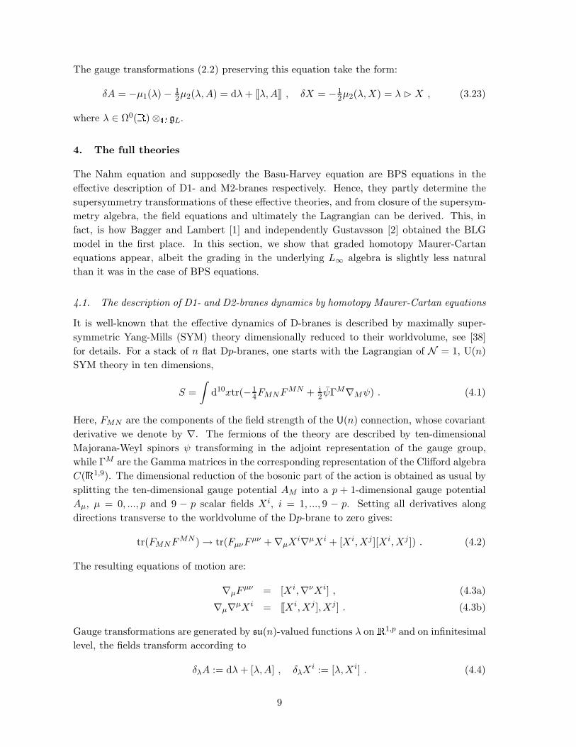
for details. For a stack of n flat Dp-branes, one starts with the Lagrangian of N = 1, U(n)

SYM theory in ten dimensions,

S =

∫

d10xtr(−14FMNF

MN + i2 ψΓM∇Mψ) . (4.1)

Here, FMN are the components of the field strength of the U(n) connection, whose covariant

derivative we denote by ∇. The fermions of the theory are described by ten-dimensional

Majorana-Weyl spinors ψ transforming in the adjoint representation of the gauge group,

while ΓM are the Gamma matrices in the corresponding representation of the Clifford algebra

C(R1,9). The dimensional reduction of the bosonic part of the action is obtained as usual by

splitting the ten-dimensional gauge potential AM into a p + 1-dimensional gauge potential

Aµ, µ = 0, ..., p and 9 − p scalar fields Xi, i = 1, ..., 9 − p. Setting all derivatives along

directions transverse to the worldvolume of the Dp-brane to zero gives:

tr(FMNFMN ) → tr(FµνF

µν + ∇µXi∇µXi + [Xi,Xj ][Xi,Xj ]) . (4.2)

The resulting equations of motion are:

∇µFµν = [Xi,∇νXi] , (4.3a)

∇µ∇µXi = [[Xi,Xj ],Xj ] . (4.3b)

Gauge transformations are generated by su(n)-valued functions λ onR1,p and on infinitesimal

level, the fields transform according to

δλA := dλ+ [λ,A] , δλXi := [λ,Xi] . (4.4)

9

It has been shown in [26] that the pure Yang-Mills equations can be interpreted as ho-

motopy Maurer-Cartan equations using a BRST complex. Earlier, in [25], the maximally

supersymmetric Yang-Mills were recast into hMC form using a pure spinor formulation.

Here, we will present a simple reinterpretation of the N = 8 SYM equations in two or three5

dimensions as hMC equations without invoking more than classical structures. To be concise,

we first discuss the purely bosonic part of the action in detail; the necessary modifications

for the supersymmetric extension will be listed in the next section.

The main difference to the Nahm and the Basu-Harvey equations is the fact that the

differential equations (4.3) are non-linear. We will therefore have to define µ1 as a non-linear

differential operator. It should be stressed, that our rewriting of the two-dimensional N = 8

SYM equations as homotopy Maurer-Cartan equations is by no means unique.

On R1,p, we consider the de Rham differential d, the Hodge operator ∗ with respect to

the Minkowski metric ηµν and the top form ω = dx0 ∧ . . . ∧ dxp. Furthermore, let q = 9 − p

as a shorthand and, as before, C(Rq) = C0(Rq) ⊕ ... ⊕ Cq(Rq) is the Clifford algebra with

generators e1, ..., eq and e := e1e2...eq. The vector space underlying our L∞ structure L for

SYM theory will be the same as for the Nahm equation extended to the two-dimensional

world-volume of the Dp-branes, and we employ again the 2-Lie algebra L = su(N). The L∞algebra will be supported on the infinite-dimensional vector space:

L := L0 ⊕ L1 ⊕ L2 , (4.5)

where:L0 := Ω0(R1,p) ⊗C L ,

L1 :=[

Ω1(R1,p) ⊗C L]

⊕[

Ω0(R1,p) ⊗C C1(Rq) ⊗ L]

,

L2 :=[

Ω1(R1,p) ⊗C Cq(Rq) ⊗ L]

⊕[

Ω2(R1,p) ⊗C C1(Rq) ⊗ L]

.

(4.6)

We view L as a Z-graded vector space whose grading is concentrated in degrees 0,1 and 2,

with L0,L1 and L2 playing the role of homogeneous subspaces of the corresponding degree.

For what follows, we consider objects:

A ∈ Ω1(R1,p) ⊗C gL , X ∈ Ω0(R1,p) ⊗C C1(Rq) ⊗ L , λ, λ1,2 ∈ Ω0(R1,p) ⊗C gL . (4.7)

We will treat A as a connection one-form on the wordlvolume valued in the trivial prin-

cipal bundle G defined by the Lie group with Lie algebra gL, X as a section of the triv-

ial vector bundle with fiber C1(Rq) ⊗ L associated with G via the representation induced

by ⊲ and λ as a generator of the group of gauge transformations of G. For these fields,

we now define various higher products µk. The modified Koszul rule of the L∞ products

gives the relations µ2(X,A) = µ2(A,X), µ3(X,X,A) = µ3(X,A,X) = µ3(A,X,X) and

µ3(A,A,X) = µ3(A,X,A) = µ3(X,A,A). Thus the homotopy Maurer-Cartan equation for

L with field φ = X +A is

− µ1(X) − µ1(A) − 12µ2(X,X) − 1

2µ2(A,A) − µ2(X,A)+

+ 16µ3(X,X,X) + 1

6µ3(A,A,A) + 12µ3(X,A,X) + 1

2µ3(A,A,X) = 0 .(4.8)

5Of course, our approach can be easily extended to arbitrary SYM theories.

10

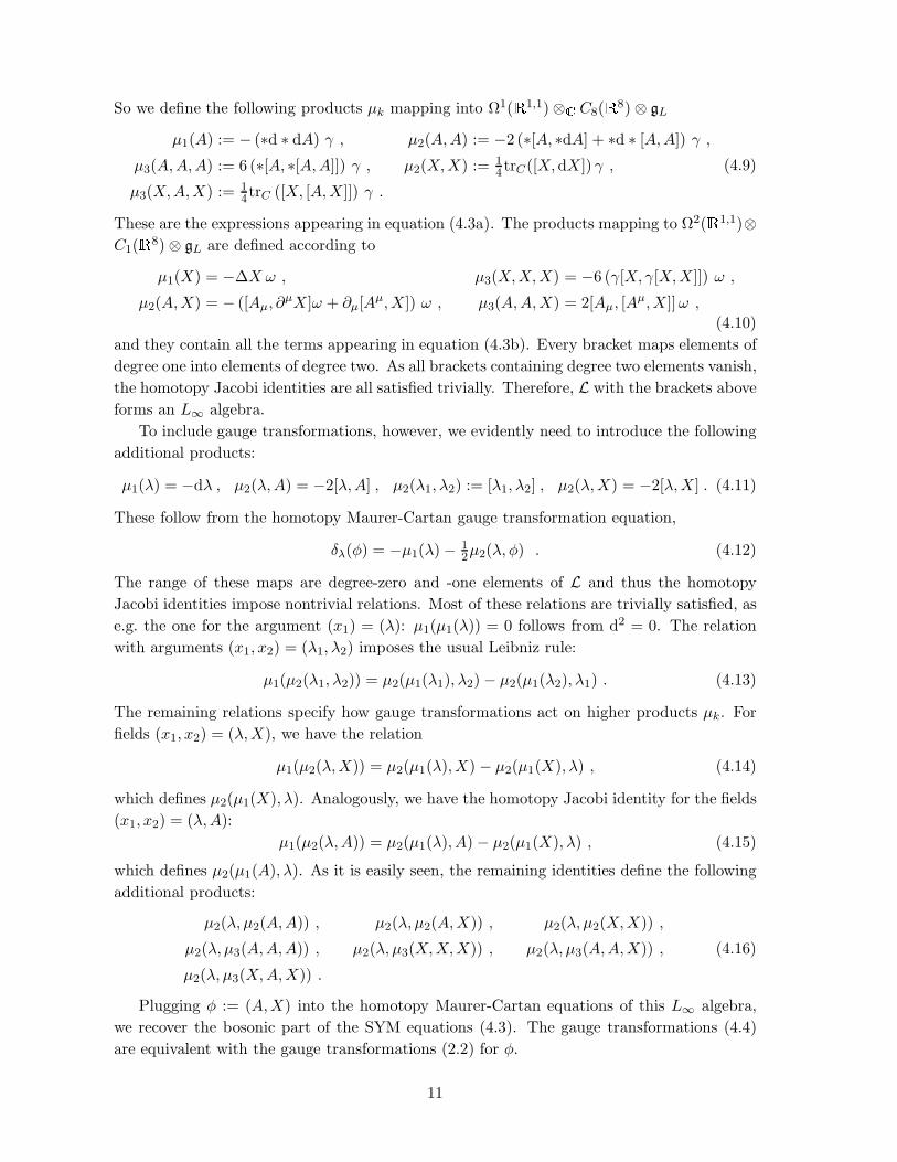
So we define the following products µk mapping into Ω1(R1,1) ⊗C C8(R8) ⊗ gL

µ1(A) := − (∗d ∗ dA) γ , µ2(A,A) := −2 (∗[A, ∗dA] + ∗d ∗ [A,A]) γ ,

µ3(A,A,A) := 6 (∗[A, ∗[A,A]]) γ , µ2(X,X) := 14 trC([X,dX]) γ ,

µ3(X,A,X) := 14trC ([X, [A,X]]) γ .

(4.9)

These are the expressions appearing in equation (4.3a). The products mapping to Ω2(R1,1)⊗C1(R8) ⊗ gL are defined according to

µ1(X) = −∆X ω , µ3(X,X,X) = −6 (γ[X, γ[X,X]]) ω ,

µ2(A,X) = − ([Aµ, ∂µX]ω + ∂µ[Aµ,X]) ω , µ3(A,A,X) = 2[Aµ, [A

µ,X]]ω ,

(4.10)

and they contain all the terms appearing in equation (4.3b). Every bracket maps elements of

degree one into elements of degree two. As all brackets containing degree two elements vanish,

the homotopy Jacobi identities are all satisfied trivially. Therefore, L with the brackets above

forms an L∞ algebra.

To include gauge transformations, however, we evidently need to introduce the following

additional products:

µ1(λ) = −dλ , µ2(λ,A) = −2[λ,A] , µ2(λ1, λ2) := [λ1, λ2] , µ2(λ,X) = −2[λ,X] . (4.11)

These follow from the homotopy Maurer-Cartan gauge transformation equation,

δλ(φ) = −µ1(λ) − 12µ2(λ, φ) . (4.12)

The range of these maps are degree-zero and -one elements of L and thus the homotopy

Jacobi identities impose nontrivial relations. Most of these relations are trivially satisfied, as

e.g. the one for the argument (x1) = (λ): µ1(µ1(λ)) = 0 follows from d2 = 0. The relation

with arguments (x1, x2) = (λ1, λ2) imposes the usual Leibniz rule:

µ1(µ2(λ1, λ2)) = µ2(µ1(λ1), λ2) − µ2(µ1(λ2), λ1) . (4.13)

The remaining relations specify how gauge transformations act on higher products µk. For

fields (x1, x2) = (λ,X), we have the relation

µ1(µ2(λ,X)) = µ2(µ1(λ),X) − µ2(µ1(X), λ) , (4.14)

which defines µ2(µ1(X), λ). Analogously, we have the homotopy Jacobi identity for the fields

(x1, x2) = (λ,A):

µ1(µ2(λ,A)) = µ2(µ1(λ), A) − µ2(µ1(X), λ) , (4.15)

which defines µ2(µ1(A), λ). As it is easily seen, the remaining identities define the following

additional products:

µ2(λ, µ2(A,A)) , µ2(λ, µ2(A,X)) , µ2(λ, µ2(X,X)) ,

µ2(λ, µ3(A,A,A)) , µ2(λ, µ3(X,X,X)) , µ2(λ, µ3(A,A,X)) ,

µ2(λ, µ3(X,A,X)) .

(4.16)

Plugging φ := (A,X) into the homotopy Maurer-Cartan equations of this L∞ algebra,

we recover the bosonic part of the SYM equations (4.3). The gauge transformations (4.4)

are equivalent with the gauge transformations (2.2) for φ.

11

4.2. Supersymmetric extension

For brevity, we do not rewrite Majorana-Weyl spinors ψ of SO(1, 9) in terms of multiple

spinors of SO(1, p), but work with the restriction S =√K of the spinor bundle over R1,9 toR1,p. Thus, we split the generators ΓM of C(R1,9) into Γµ, µ = 0, ..., p and eI , I = 1, ..., q.

In this form, the N = 8 SYM equations in two or three dimensions read as

∇µFµν = [XI ,∇νXI ] − 1

2Γναβψα, ψβ , (4.17a)

Γµαβ∇µψ

β = −ΓIαβ[XI , ψβ ] , (4.17b)

∇µ∇µXI = [[XI ,XJ ],XJ ] − 12ΓI

αβψα, ψβ . (4.17c)

In the homotopy Maurer-Cartan equations, we take φ = (A,ψ, ψ,X), where ψ ∈ Γ(S) and

ψ ∈ Γ(S). We therefore extend L to

L := Ω•(R1,p) ⊗C C(Rq) ⊗ gL ⊕(

Γ(S) ⊕ Γ(S) ⊕ Γ(S∗) ⊕ Γ(S∗))

⊗ gL , (4.18)

which we associate with the following grading:

deg(Γ(S) ⊗ gL) = deg(Γ(S) ⊗ gL) = 1 , deg(Γ(S∗) ⊗ gL) = deg(Γ(S∗) ⊗ gL) = 2 . (4.19)

The additional products we have to introduce are straightforwardly read off the equations of

motion (4.17):

µ1(ψ) = −Γµαβ∂µψ

β , µ2(A,ψ) = −ΓµαβAµψ

β ,

µ2(X,ψ) = −ΓIαβ[XI , ψβ ] , µ2(ψ, ψ) = −1

2ηµνΓµαβψα, ψβdxν − 1

2ΓIΓIαβψα, ψβω .

(4.20)

The homotopy Jacobi identities are again trivially satisfied, as a product µk1having another

bracket µk2amongst its arguments is defined to be vanishing.

To capture gauge transformations, we additionally introduce

µ2(λ, ψ) := −2[λ, ψ] . (4.21)

The homotopy Jacobi identities then extend the action of gauge transformations to products

µk containing ψ in the arguments.

The homotopy Maurer-Cartan equations together with the L∞ algebra L endowed with

all of these brackets reproduce both the two-dimensional N = 8 SYM equations and the

associated gauge transformations of the fields.

Note that the association of degrees to the various subspaces of L seems to be rather

ad-hoc. A more enlightening approach to the grading of the L∞ algebra is obtained from

considering ghost number grading of a BRST complex, as done for pure Yang-Mills theory

in [26].

4.3. Review of the BLG theory

We start from a metric 3-Lie algebra (L, ( , )) with associated Lie algebra gL. The bracket

and the metric on L can be used to construct an invariant bilinear form (( , )) on gL, which

is not identical with the Killing form on gL, and which is not positive definite [10]:

((x1 ∧ x2, b1 ∧ b2)) := ([x1, x2, b1], b2) , x1, x2, b1, b2 ∈ L . (4.22)

12

One easily verifies symmetry of (( , )).

The matter field content of the BLG theory is given by the Goldstone fields arising from

the spacetime symmetries broken by the presence of the M2-branes. We have thus 8 scalar

fields XI , I = 1, ..., 8 and a Majorana spinor Ψ of Spin(1, 10) as their superpartner. The

matter fields take values in the 3-Lie algebra L with invariant form ( , ). In addition,

we have a gauge potential Aµ taking values in Ω1(R1,2) ⊗C gL. As gamma matrices, we

use the 11-dimensional ones, which are split according to ΓM , M = 0, ..., 10 → (Γµ, eI),

(µ = 0, .., 2, I = 1, ..., 8). For simplicity, we introduce X = eIXI and the invariant form ( , )

is assumed to include a trace where necessary. The Lagrangian density can then be written

in the form:

LBLG = − 12(∇µX,∇µX)A⊗C + i

2(Ψ,Γµ∇µΨ)A + i4 (Ψ, [X,X,Ψ])A

− 112([X,X,X], [X,X,X])A⊗C + 1

2εµνκ

(

((Aµ, ∂νAκ)) + 13((Aµ, [[Aν , Aκ]]))

)

.(4.23)

where [[ , ]] denotes the Lie bracket in gL, ⊲ denotes the natural action of elements of gL

on L and [ , , ] is the triple bracket in L extended linearly for C(R8)-valued objects. This

action is invariant under the supersymmetry transformations

δX = iΓI εΓIΨ , δΨ = ∇µXΓµε− 1

6 [X,X,X]ε , δAµ = iεΓµ(X ∧ Ψ) (4.24)

up to translations, equations of motion and gauge transformations. On infinitesimal level,

the latter are generated by λ ∈ Ω0(R1,2) ⊗C gL according to

δX = λ ⊲ X , δΨ = λ ⊲ Ψ , δAµ = ∂µλ+ [[λ,Aµ]] . (4.25)

4.4. BLG equations as homotopy Maurer-Cartan equations

The BLG equations can also be rewritten as homotopy Maurer-Cartan equations; as the

equations of motion for the gauge field are of Chern-Simons type, the grading is slightly

more natural than in the case of SYM theory. As before, let us first discuss the bosonic

part in detail and add the supersymmetric extension later. The equations of motion take the

form:∇µ∇µX + 1

2e[X,X, e[X,X,X]] = 0 ,

[∇µ,∇ν ] + εµνκ(XJ ∧ (∇κXJ)) = 0 .(4.26)

The appropriate extension for the algebra underlying the homotopy Maurer-Cartan in-

terpretation of the Basu-Harvey equation tuns out to be

L := Ω•(R1,2) ⊗C C(R8) ⊗ FL , (4.27)

and we associate the following degrees to its subspaces

deg(Ω0(R1,2) ⊗ gL) = 0 ,

deg(Ω1(R1,2) ⊗ gL) = deg(Ω0(R1,2) ⊗ C1(R8) ⊗ L) = 1 ,

deg(Ω2(R1,2) ⊗ gL) = deg(Ω3(R1,2) ⊗ C1(R8) ⊗ L) = 2 .

(4.28)

Our notation for elements of the various subspaces will be

A ∈ Ω1(R1,2) ⊗C gL , X ∈ Ω0(R1,2) ⊗C C1(R8) ⊗C L , λ, λ1,2 ∈ Ω0(R1,2) ⊗C gL . (4.29)

13

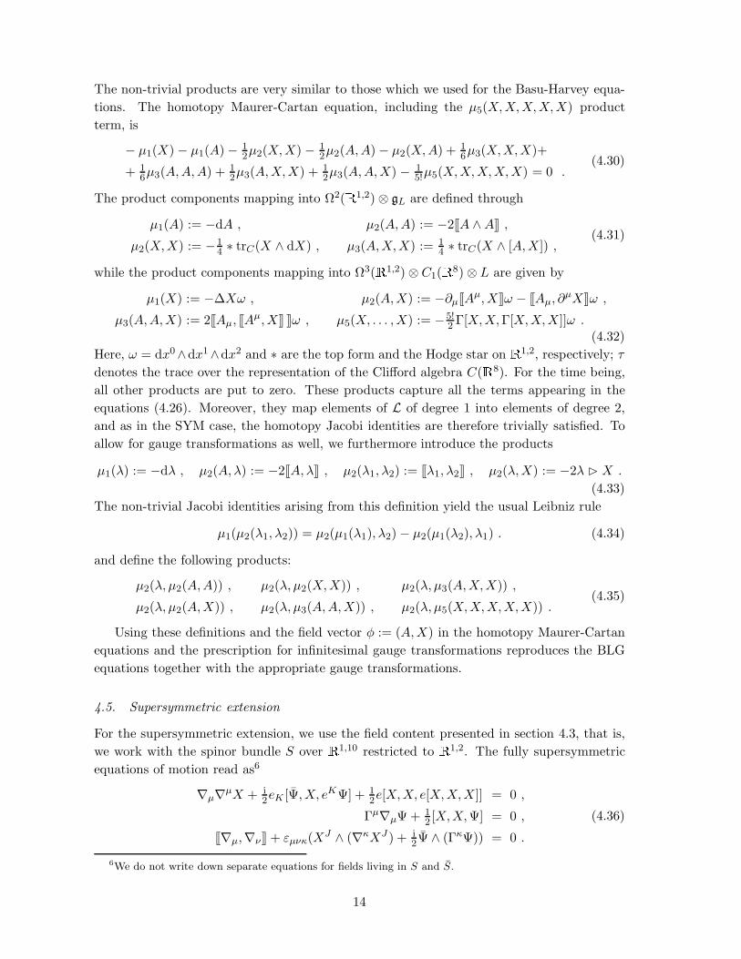
The non-trivial products are very similar to those which we used for the Basu-Harvey equa-

tions. The homotopy Maurer-Cartan equation, including the µ5(X,X,X,X,X) product

term, is

− µ1(X) − µ1(A) − 12µ2(X,X) − 1

2µ2(A,A) − µ2(X,A) + 16µ3(X,X,X)+

+ 16µ3(A,A,A) + 1

2µ3(A,X,X) + 12µ3(A,A,X) − 1

5!µ5(X,X,X,X,X) = 0 .(4.30)

The product components mapping into Ω2(R1,2) ⊗ gL are defined through

µ1(A) := −dA , µ2(A,A) := −2[[A ∧A]] ,

µ2(X,X) := −14 ∗ trC(X ∧ dX) , µ3(A,X,X) := 1

4 ∗ trC(X ∧ [A,X]) ,(4.31)

while the product components mapping into Ω3(R1,2) ⊗ C1(R8) ⊗ L are given by

µ1(X) := −∆Xω , µ2(A,X) := −∂µ[[Aµ,X]]ω − [[Aµ, ∂µX]]ω ,

µ3(A,A,X) := 2[[Aµ, [[Aµ,X]] ]]ω , µ5(X, . . . ,X) := −5!

2 Γ[X,X,Γ[X,X,X]]ω .(4.32)

Here, ω = dx0∧dx1∧dx2 and ∗ are the top form and the Hodge star on R1,2, respectively; τ

denotes the trace over the representation of the Clifford algebra C(R8). For the time being,

all other products are put to zero. These products capture all the terms appearing in the

equations (4.26). Moreover, they map elements of L of degree 1 into elements of degree 2,

and as in the SYM case, the homotopy Jacobi identities are therefore trivially satisfied. To

allow for gauge transformations as well, we furthermore introduce the products

µ1(λ) := −dλ , µ2(A,λ) := −2[[A,λ]] , µ2(λ1, λ2) := [[λ1, λ2]] , µ2(λ,X) := −2λ ⊲ X .

(4.33)

The non-trivial Jacobi identities arising from this definition yield the usual Leibniz rule

µ1(µ2(λ1, λ2)) = µ2(µ1(λ1), λ2) − µ2(µ1(λ2), λ1) . (4.34)

and define the following products:

µ2(λ, µ2(A,A)) , µ2(λ, µ2(X,X)) , µ2(λ, µ3(A,X,X)) ,

µ2(λ, µ2(A,X)) , µ2(λ, µ3(A,A,X)) , µ2(λ, µ5(X,X,X,X,X)) .(4.35)

Using these definitions and the field vector φ := (A,X) in the homotopy Maurer-Cartan

equations and the prescription for infinitesimal gauge transformations reproduces the BLG

equations together with the appropriate gauge transformations.

4.5. Supersymmetric extension

For the supersymmetric extension, we use the field content presented in section 4.3, that is,

we work with the spinor bundle S over R1,10 restricted to R1,2. The fully supersymmetric

equations of motion read as6

∇µ∇µX + i2eK [Ψ,X, eKΨ] + 1

2e[X,X, e[X,X,X]] = 0 ,

Γµ∇µΨ + 12 [X,X,Ψ] = 0 ,

[[∇µ,∇ν ]] + εµνκ(XJ ∧ (∇κXJ ) + i2Ψ ∧ (ΓκΨ)) = 0 .

(4.36)

6We do not write down separate equations for fields living in S and S.

14

To incorporate the fermions, we need to extend L as follows

L := Ω•(R1,2) ⊗C C(R8) ⊗ FL ⊕ (Γ(S) ⊕ Γ(S) ⊕ Γ(S∗) ⊕ Γ(S∗)) ⊗ L , (4.37)

and introduce the further products

µ2(Ψ,Ψ) := i2εµνκΨ ∧ (ΓκΨ)dxµ ∧ dxν , µ3(X,X,Ψ) := 1

2 [X,X,Ψ] ,

µ3(Ψ,X,Ψ) := i2eK [Ψ,X, eKΨ] .

(4.38)

These are enough to fully capture the equations of motion, and to allow for gauge transfor-

mations, we extend the set of defined products by

µ2(λ,Ψ) := −2[λ,Ψ] . (4.39)

The homotopy Jacobi identities then define for us the action of µ2(λ, ) on any of the products

(4.38), and thus the description of the BLG equations together with their gauge symmetry

in terms of homotopy Maurer-Cartan equations is complete.

4.6. From M2-branes to D2-branes

In [4], a nice reduction mechanism was proposed to descend from the BLG model with 3-Lie

algebra A4 describing two M2-branes to d = 3, N = 8 SYM theory with gauge group U(2)

describing two D2-branes. The idea behind this is to compactify one direction, say x10 on

a circle and to assume that this compactification associates an expectation value with the

corresponding scalar X 8 = X4 8τ4:

〈X4 8〉 =R

ℓ3/2p

=gs

ℓs= gY M , (4.40)

where τa, a = 1, ..., 4 denote the generators of A4. This induces a splitting X I → (XI , gY M )

as well as a splitting

f abcd = εabcd = εabcδd4 − εabdδc4 + εacdδb4 − εbcdδa4 , a, b, c, d = 1, ..., 3 . (4.41)

Because of the last decomposition, we can split the gauge potential according to Aµ :=

Aabµ τa ∧ τb

Aaµ := Aa4

µ and Baµ := 1

2εabcA

bcµ . (4.42)

Rewriting the hMC equations of the BLG model using the expectation value for X 8 as well as

the decomposition of the gauge potential, the equations of motion for Baµ become algebraic,

and we can eliminate this field. The result are the hMC equations of d = 3 N = 8 SYM

theory plus corrections in lower powers of gY M . In a strong coupling expansion, in which

the subleading terms are neglected, the corrections vanish, and the effective description of a

stack of two D2-branes is reproduced [4].

Acknowledgements

DM and AZ are supported by IRCSET (Irish Research Council for Science, Engineering and

Technology) postgraduate research scholarships. CS is supported by an IRCSET postdoctoral

fellowship.

15

Appendix: Various extensions of the notion of a Lie algebra

In this appendix, we give a brief account of the various higher Lie structures used in this

paper, which in particular fixes our conventions.

Notations. Let Sn be the group of permutations on n elements. Given a permutation

σ ∈ Sn, we let ǫ(σ) denote its signature. Recall that σ is called an (j, n− j)-unshuffle (where

1 ≤ j ≤ n) if σ(1) < ... < σ(j) and σ(j + 1) < ... < σ(n). We let Sh(i, n − i) denote the set

of all (i, n− i)-unshuffles.

A. Ungraded extensions of the notion of Lie algebra

Let k be a field of characteristic zero, for example k = R or k = C and R be an associative

and commutative unital k-algebra, for example R = R or R = C again.

n-Lie algebras in the sense of Filippov

Definition. An n-Lie algebra over R is a (unital) R-module L endowed with an R-multili-

near map [ , . . . , ] : L×n → L such that:

(a) [ , . . . , ] is totally antisymmetric, i.e.

[x1, . . . , xn] = ǫ(σ)[xσ(1), . . . , xσ(n)] , for all σ ∈ Sn and all x1 . . . xn ∈ L (A.1)

(b) [ , . . . , ] satisfies the following fundamental identity for all xi, yj ∈ L, i = 1, ..., n −1, j = 1, ..., n:

[x1, . . . , xn−1, [y1, . . . , yn]] =

n∑

i=1

[y1, . . . , yi−1, [x1, . . . , xn−1, yi], yi+1, . . . , yn] . (A.2)

Notice that 2-Lie algebras are ordinary Lie algebras, for which the fundamental identity

(A.2) corresponds to the usual Jacobi identity. A basic example is the n-Lie algebra An+1

over R whose underlying vector space is an oriented Euclidean vector space of dimension

n+ 1 and whose n-bracket is given by the cross product of an ordered system of n vectors:

[x1, ..., xn] := x1 × . . . × xn :=

∣

∣

∣

∣

∣

∣

∣

x11 ... x1

n e1... ... ... ...

xn+11 ... xn+1

n en+1

∣

∣

∣

∣

∣

∣

∣

, (A.3)

In the last equality, e1, ..., en+1 is any orthonormal basis of An+1 and xi =∑n+1

j=1 xjiej with

xji ∈ R. The 3-Lie algebra A4 played an important role in the BLG model, see e.g. [2].

Let us fix an n-Lie algebra L. Any such algebra defines an ordinary Lie bracket [[ , ]]

(called the associated basic bracket) on the R-module gL := ∧n−1R L via:

[[x1∧ . . .∧xn−1, y1∧ ...∧yn−1]] :=

n−1∑

i=1

(y1∧ . . .∧yi−1∧ [x1 . . . xn−1, yi]∧yi+1∧ . . .∧yn−1) (A.4)

The ordinary Lie R-algebra (gL, [[ , ]]) is called the basic Lie algebra of L.

16

Definition. An R-linear map D : L→ L is called a derivation of L if:

D([x1, . . . , xn]) =

n∑

i=1

[x1, . . . , xi−1,D(xi), xi+1, . . . , xn] (A.5)

for any x1, . . . , xn ∈ L.

The space DerR(L) of all R-linear derivations of L is an ordinary Lie R-algebra with Lie

bracket given by the commutator of derivations. For any elements x1 . . . xn−1 of L, we define

a linear map Dx1...xn−1: L→ L through:

Dx1...xn−1(x) = [x1, . . . , xn−1, x] (x ∈ L) . (A.6)

It is easy to check that Dx1...xn−1is a derivation of L, called the inner derivation defined

by the sequence of elements x1 . . . xn−1. Indeed, Filippov’s fundamental (A.2) identity is

equivalent with the derivation property:

Dx1...xn−1([y1, ..., yn]) =

n∑

i=1

[y1, . . . , yi−1,Dx1,...,xn−1(yi), yi+1, . . . , yn] . (A.7)

Relation (A.7) implies:

[

Dx1...xn−1,Dy1...yn−1

]

=

n−1∑

i=1

Dy1,...,yi−1,Dx1,...,xn−1(yi),yi+1,...yn−1

, (A.8)

which shows that the subspace InnR(L) of inner R-linear derivations is a Lie subalgebra of

DerR(L).

Since the map (x1 . . . xn−1) ∈ L×(n−1) D→ Dx1...xn−1∈ DerR(L) is R-multilinear and

alternating, it factors through an R-linear map gLD→ DerR(L), whose value on an element

u ∈ G we denote by Du := D(u) ∈ DerR(L). Consequently, we can write (A.7) as:

[Dx1∧...∧xn−1, Dy1∧...,∧yn−1

] = D[[y1∧...∧yn−1,x1∧...xn−1]] , (A.9)

which shows that D is a linear representation (called the canonical representation) of the

basic algebra on the underlying vector space of L. The Lie algebra of inner derivations is

the image of this representation, i.e. we have InnR(L) = ImD. The action of u ∈ gL on an

element x ∈ L will be denoted by:

u ⊲ x := Du(x) . (A.10)

The fact that the representation D of gL on L acts through derivations of (L, [ , . . . , ]) is

equivalent with the statement that the n-bracket [ , . . . , ] satisfies Filippov’s fundamental

identity (A.2).

17

The algebra FL. When L is an ordinary Lie algebra with bracket [ , ], then we have

[[ , ]] = [ , ] and gL coincides with L as a Lie algebra. In this case, the representation D of gL in

L is the adjoint representation ad of L in itself. The fact that ad acts in L through derivations

of (L, [ , ]) is the well-known reformulation of the classical Jacobi identity. Filippov’s notion

of n-Lie algebra is inspired by generalizing this take on the classical Jacobi identity.

Let L be an n-Lie algebra with n > 2. Since we have an action of gL on L, the R-module

FL := gL⊕L carries an algebraic structure consisting of two R-bilinear and alternating maps,

namely a 2-bracket [ , ] : FL × FL → FL and an n-bracket [ , . . . , ] : F×nL → FL, defined as

follows for all u, v, u1 . . . un ∈ gL and all x, y, x1 . . . xn ∈ L:

[u+ x, v + y] := [u, v] + u ⊲ y − v ⊲ x ,

[u1 + x1 . . . un + xn] := [x1, . . . , xn]

+

n∑

i=1

(−1)i−1[[ui, x1 ∧R . . . ∧R xi−1 ∧R xi+1 ∧R . . . ∧R xn]] .

We will see later that the triple (FL, [ , ], [ , . . . , ]) is an (ungraded) L2,n algebra over R.

Definition. A map η : L× L→ R on L is called invariant if:

η(D(x), y) + η(x,D(y)) = 0 for all x, y ∈ L and all D ∈ InnR(L) . (A.11)

Notice that condition (A.11) amounts to:

η([z1, ..., zn−1, x], y) + η(x, [z1, ..., zn−1, y]) = 0 ∀x, y, z1 . . . zn−1 ∈ L . (A.12)

Definition. When L is an n-Lie algebra over C, then a Hermitian metric on L is an

invariant Hermitian form ( , ) : L× L→ C.

Lie n-algebras

Definition. A Lie n-algebra over R is an R-module L endowed with an R-multilinear map

µn := [ , . . . , ] : L×n → L which is totally antisymmetric:

[x1, . . . , xn] = ǫ(σ)[xσ(1), . . . , xσ(n)] , (xi ∈ L) (A.13)

and satisfies the homotopy Jacobi identity:

∑

σ∈Sh(n,n−1)

ǫ(σ)[[xσ(1) , ..., xσ(n−1), xσ(n)], xσ(n+1)..., xσ(2n−1)] = 0 (xi, yj ∈ L) . (A.14)

The definition given above coincides with that used by Hanlon and Wachs [30] but differs

from that used e.g. in [39]. The following result was proved by Dzhumadil’daev7:

7In fact, Dzhumadil’daev also shows that n-Lie algebras as so-called “symmetric algebras”, which in turn

are Lie n-algebras.

18

Proposition. [31] Filippov’s fundamental identity (A.2) implies the homotopy Jacobi iden-

tity, i.e. any n-Lie algebra (L, [ , . . . , ]) is also a Lie n-algebra. Dzhumadil’daev also shows

that the converse statement is untrue, a counterexample being provided by Jacobian algebras,

which are Lie n-algebras but not n-Lie.

As we shall see below, Lie n-algebras are the same as ungraded Ln algebras, a particular

case of ungraded L∞ algebras. Hence Dzhumadil’daev’s result above shows that the theory

of n-Lie algebras is a special case of the theory of L∞ algebras..

L∞ algebras

Definition. An (ungraded) L∞ (or strong homotopy Lie) algebra over R is an R-module

L endowed with a family of R-multilinear maps µn : L×n → L (n ≥ 1) such that:

(1) Each µn is alternating, i.e.:

µn(xσ(1) . . . xσ(n)) = ǫ(σ)µn(x1 . . . xn) for all x1 . . . xn ∈ L (A.15)

(2) Each of the following countable tower of ungraded L∞ identities is satisfied:

n∑

i=1

∑

σ∈Sh(i,n−i)

(−1)i(n+1)ǫ(σ)µn−i+1(µi(xσ(1), ..., xσ(i)), xσ(i+1), ..., xσ(n)) = 0 (A.16)

for all n ≥ 1 and all x1, ..., xn ∈ L.

Definition. Let S ⊂ N∗ be a proper subset of the set N∗ of all non-vanishing natural

numbers. An (ungraded) LS algebra over R is an L∞ algebra over R whose products µi

vanish for i /∈ S.

Thus an LS algebra has only the products µn with n ∈ S, and some of the identities

(A.16) might be trivially satisfied. Some particular cases which are common in practice are

the following:

(1) S = 1 . . . n for some n ≥ 1. In this case, and LS algebra is also called an L(n)

algebra. Such an L∞ algebra has only the products µ1 . . . µn, and one need only consider the

first 2n − 1 identities in (A.16) (those with k = 1 . . . 2n− 1) since all identities with k ≥ 2n

are satisfied trivially.

(2) S = n for some n ∈ N∗. Such an LS algebra is also called an Ln algebra. An Ln

algebra has only the product µn and the only nontrivial identity in (A.16) is the one with

k = 2n− 1:

∑

σ∈Sh(n,n−1)

ǫ(σ)µn(µn(xσ(1), ..., xσ(n)), xσ(n+1), ..., xσ(2n−1)) = 0 ∀x1, ..., x2n−1 ∈ L . (A.17)

This is called the homotopy Jacobi identity (it is also the last nontrivial identity of an

L(n) algebra). Clearly any Ln algebra is also an L(n) algebra.

Remark. It is obvious from the definitions above that a Lie n-algebra is the same as an

(ungraded) Ln algebra.

19

Examples. (1) An L(1) algebra L has just one linear map µ1 and (A.16) reduce to the

single condition µ1 µ1 = 0, i.e. (L,µ1) is a differential space. Clearly an L1 algebra is the

same thing as an L(1) algebra.

(2) An L(2) algebra has a linear unary product µ1 of weak degree and bilinear binary

product µ2, the second being alternating. Conditions (A.16) say that µ1 squares to zero,

that it is a derivation of µ2:

µ1(µ2(x1, x2)) = µ2(µ1(x1), x2) + µ2(x1, µ1(x2)) (A.18)

and that µ2 satisfies the Jacobi identity:

µ2(µ2(x1, x2), x3) + µ2(µ2(x2, x3), x1) + µ2(µ2(x3, x1), x2) = 0 (A.19)

These constraints state that (L,µ1, µ2) is a differential Lie algebra. An L2 algebra is an

L(2) algebra with trivial differential, i.e. an ordinary Lie algebra.

(3) An L2,n algebra has an alternating 2-bracket µ2 = [ , ] and an alternating n-bracket

µn = [ , . . . , ]. Conditions (A.16) amount to the following constraints:

(a) [ , ] is a Lie bracket

(b) [ , . . . , ] satisfies homotopy Jacobi

(c) The following identity is satisfied for all elements of the L2,n algebra

∑

1≤i<j≤n+1

(−1)i+j+1[[xi, xj ], x1, . . .xi, . . . , xj , . . . xn+1]+

+

n+1∑

i=1

(−1)n+i−1[[x1, . . . , xi, . . . , xn], xi] = 0

(A.20)

B. The graded versions

Preparations. Let G be an Abelian group and fix a group morphism φ : G→ Z2. Recall

that a G-graded R-modules is an R-module V endowed with a submodule decomposition:

V = ⊕g∈GVg .

Given such a module, its pure (or homogeneous) elements are those elements x ∈ V for

which there exists some g = gx such that x ∈ Vg. In this case, we let deg x := g. We also

let x := φ(deg x) = φ(g) ∈ Z2, which we will call the parity of x. Thus x is even if its

parity equals 0 ∈ Z2 and odd if its parity equals 1 ∈ Z2. Notice that the sign factor (−1)g is

unambiguously defined. The reduced grading of V is the Z2-grading V = V red0

⊕V red1

defined

through:

V red0

:= ⊕g∈G|φ(g)=0Vg , V red1

:= ⊕g∈G|φ(g)=1Vg .

The tensor powers ⊗nRV of V are defined as usual, while the (G,φ)-graded symmetric and

graded exterior powers ⊙nRV and ∧n

RV are defined with sign factors induced by the parity of

homogeneous elements. All these R-modules are again G-graded.

Given a permutation σ ∈ Sn, we define the Koszul sign ǫ(σ, x1 . . . xn) of n pure elements

x1 . . . xn ∈ V via the identity:

xσ(1) ⊙R . . .⊙R xσ(n) = ǫ(σ, x1 . . . xn)x1 ⊙R . . .⊙R xn ,

20

where x1 ⊙ . . . ⊙ xn is the pure element of ⊗nRV defined by x1 . . . xn. The modified Koszul

sign χ(σ, x1 . . . xn) is defined through:

χ(σ, x1 . . . xn) := ǫ(σ)ǫ(σ, x1 . . . xn)

and we have:

xσ(1) ∧R . . . ∧R xσ(n) = χ(σ, x1 . . . xn)x1 ∧R . . . ∧R xn

Given another group morphism ψ : G→ Z2 and a (G,ψ)-graded R-module U , an R-linear

map f : V → U is called homogeneous of degree h ∈ G if f(Vg) ⊂ Ug+h for all g ∈ G. It

is called weakly homogeneous of weak homogeneity degree α ∈ Z2 if f(V redβ ) ⊂ U red

β+α for all

β ∈ Z2.

As in the Z2-graded case, we can define the notions of (G,φ)-graded symmetric and

graded antisymmetric R-multilinear maps η : V ×n → V , and find that these factor through

R-linear maps η from ⊗nRV and ∧n

RV to V , respectively.

Graded Lie algebras

Definition. A (G,φ)-graded Lie algebra over R is a (unital) G-graded R-module L endowed

with an R-bilinear map [ , ] : L×2 → L such that:

(a) [ , ] is graded antisymmetric, i.e.

[x, y] = (−1)xy[y, x] for all homogeneous elements x, y ∈ L , (B.21)

(b) [ , ] satisfies the (G,φ)-graded Jacobi identity for all homogeneous elements x, y, z ∈ L:

[x, [y, z]] + (−1)x(y+z)[y, [z, x]] + (−1)z(x+y)[z, [x, y]] = 0 . (B.22)

As for usual Lie algebras, (L, [ , ]) has an adjoint representation ad : L→ EndR(L) given

by (here adx := ad(x)):

adx(y) := [x, y] . (B.23)

A weakly homogeneous graded derivation of parity α ∈ Z2 is a homogeneous R-linear map

D : L→ L such that:

D([x, y]) = [D(x), y] + (−1)αx[x,D(y)] (B.24)

for all homogeneous x, y ∈ L. We let D := α and say that D is even if α = 1 and that D

is odd if α = 1. The set of weakly homogeneous derivations of L is denoted by DerR(L). It

is a graded Lie algebra when endowed with the usual graded commutator of homogeneous

linear operators in L, which makes it into a graded Lie subalgebra of EndR(L). For any

homogeneous element x ∈ L, the associated adjoint action adx is weakly homogeneous of

parity x, and ad gives an R-linear representation of the graded Lie algebra (L, [ , ]) on

L, i.e. ad : L → EndR(L) is a morphism of graded Lie algebras. Given this property, the

graded Jacobi identity (B.22) is equivalent to the statement that adx is a weakly homogeneous

derivation for every homogeneous element x ∈ L.

21

Graded n-Lie algebras

Definition. A (G,φ)-graded n-Lie algebra over R is a (unital) G-graded R-module L en-

dowed with an R-multilinear map [ , . . . , ] : L×n → L such that8:

(a) [ , . . . , ] is totally graded antisymmetric, i.e.

[x1, . . . , xn] = χ(σ, x1 . . . xn)[xσ(1), . . . , xσ(n)] , for all σ ∈ Sn and all x1 . . . xn ∈ L (B.25)

(b) [ , . . . , ] satisfies the following graded fundamental identity for all xi, yj ∈ L, i =

1, ..., n − 1, j = 1, ..., n:

[x1, . . . , xn−1, [y1, . . . , yn]] = (B.26)

=n

∑

i=1

(−1)(x1+...+xn−1)(y1+...+yi−1)[y1, . . . , yi−1, [x1, . . . , xn−1, yi], yi+1, . . . , yn] .

Notice that 2-Lie algebras are ordinary (G,φ)- graded Lie algebras, for which the graded

fundamental identity (B.26) becomes the usual (G,φ)-graded Jacobi identity.

Let us fix a (G,φ)-graded n-Lie algebra L. Such an algebra defines an ordinary (G,φ)-

graded Lie bracket [[ , ]] (called the associated basic bracket) on the graded R-module gL :=

∧n−1R L via:

[[x1 ∧R . . . ∧R xn−1, y1 ∧R ... ∧R yn−1]] := (B.27)

=

n−1∑

i=1

(−1)(x1+...+xn−1)(yn+...+yn+i−1)(y1 ∧ . . . ∧ yi−1 ∧ [x1 . . . xn−1, yi] ∧ yi+1 ∧ . . . ∧ yn−1)

The (G,φ)-graded Lie R-algebra (gL, [[ , ]]) is called the basic graded Lie algebra of L.

Definition. An R-linear map D : L→ L is called a weakly homogeneous derivation of L of

parity α ∈ Z2 if:

D([x1, . . . , xn]) =

n∑

i=1

(−1)α(x1+...+xi−1)[x1, . . . , xi−1,D(xi), xi+1, . . . , xn] (B.28)

for any x1, . . . , xn ∈ L. We set D := α.

The space DerR(L) of all R-linear and weakly homogeneous derivations of L is a (G,φ)-

graded Lie R-algebra with graded Lie bracket inherited from EndR(L). For any elements

x1 . . . xn−1 of L, we define a linear map Dx1...xn−1: L→ L through:

Dx1...xn−1(x) = [x1, . . . , xn−1, x] (x ∈ L) . (B.29)

When x1 . . . xn−1 are homogeneous, then it is easy to check that Dx1...xn−1is a weakly ho-

mogeneous derivation of L of parity x1 + . . . + xn−1, called the inner derivation defined by

8Here (and in the following), the given conditions hold for homogeneous elements; for other elements, they

are linearly extended.

22

the sequence of elements x1 . . . xn−1. Indeed, the graded version of Filippov’s fundamental

identity (A.2) is equivalent with the graded derivation property:

Dx1...xn−1([y1, ..., yn]) =

n∑

i=1

(−1)(x1+...+xn−1)(y1+...+yi−1)[y1, . . . , yi−1,Dx1...xn−1(yi), yi+1, . . . , yn] .

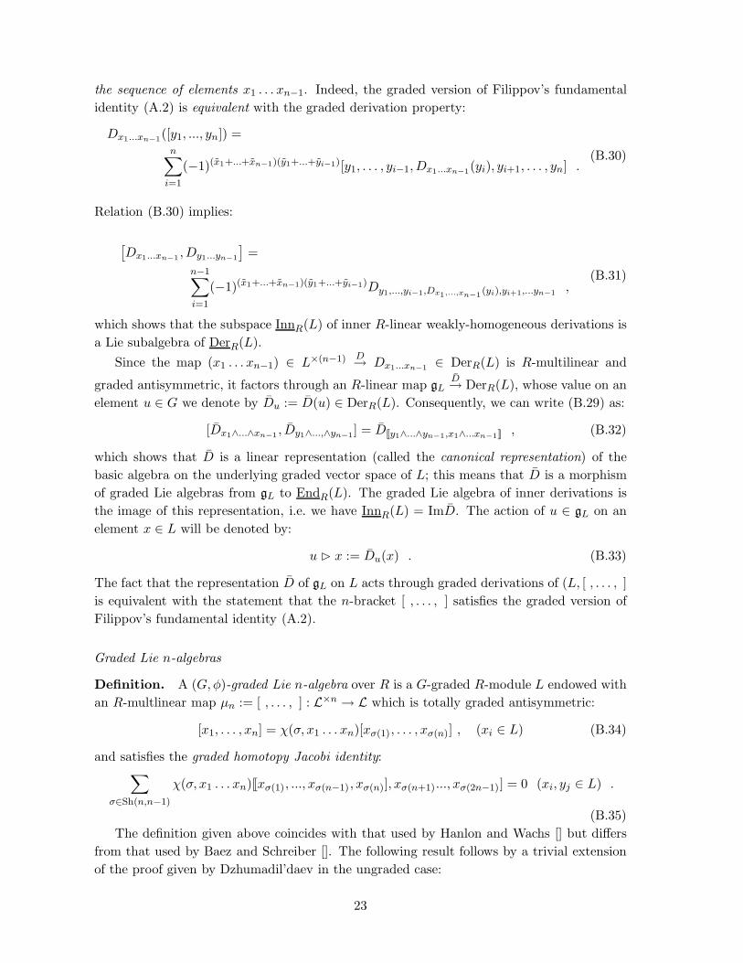
(B.30)

Relation (B.30) implies:

[

Dx1...xn−1,Dy1...yn−1

]

=

n−1∑

i=1

(−1)(x1+...+xn−1)(y1+...+yi−1)Dy1,...,yi−1,Dx1,...,xn−1(yi),yi+1,...yn−1

,(B.31)

which shows that the subspace InnR(L) of inner R-linear weakly-homogeneous derivations is

a Lie subalgebra of DerR(L).

Since the map (x1 . . . xn−1) ∈ L×(n−1) D→ Dx1...xn−1∈ DerR(L) is R-multilinear and

graded antisymmetric, it factors through an R-linear map gLD→ DerR(L), whose value on an

element u ∈ G we denote by Du := D(u) ∈ DerR(L). Consequently, we can write (B.29) as:

[Dx1∧...∧xn−1, Dy1∧...,∧yn−1

] = D[[y1∧...∧yn−1,x1∧...xn−1]] , (B.32)

which shows that D is a linear representation (called the canonical representation) of the

basic algebra on the underlying graded vector space of L; this means that D is a morphism

of graded Lie algebras from gL to EndR(L). The graded Lie algebra of inner derivations is

the image of this representation, i.e. we have InnR(L) = ImD. The action of u ∈ gL on an

element x ∈ L will be denoted by:

u ⊲ x := Du(x) . (B.33)

The fact that the representation D of gL on L acts through graded derivations of (L, [ , . . . , ]

is equivalent with the statement that the n-bracket [ , . . . , ] satisfies the graded version of

Filippov’s fundamental identity (A.2).

Graded Lie n-algebras

Definition. A (G,φ)-graded Lie n-algebra over R is a G-graded R-module L endowed with

an R-multlinear map µn := [ , . . . , ] : L×n → L which is totally graded antisymmetric:

[x1, . . . , xn] = χ(σ, x1 . . . xn)[xσ(1), . . . , xσ(n)] , (xi ∈ L) (B.34)

and satisfies the graded homotopy Jacobi identity:∑

σ∈Sh(n,n−1)

χ(σ, x1 . . . xn)[[xσ(1), ..., xσ(n−1) , xσ(n)], xσ(n+1)..., xσ(2n−1)] = 0 (xi, yj ∈ L) .

(B.35)

The definition given above coincides with that used by Hanlon and Wachs [] but differs

from that used by Baez and Schreiber []. The following result follows by a trivial extension

of the proof given by Dzhumadil’daev in the ungraded case:

23

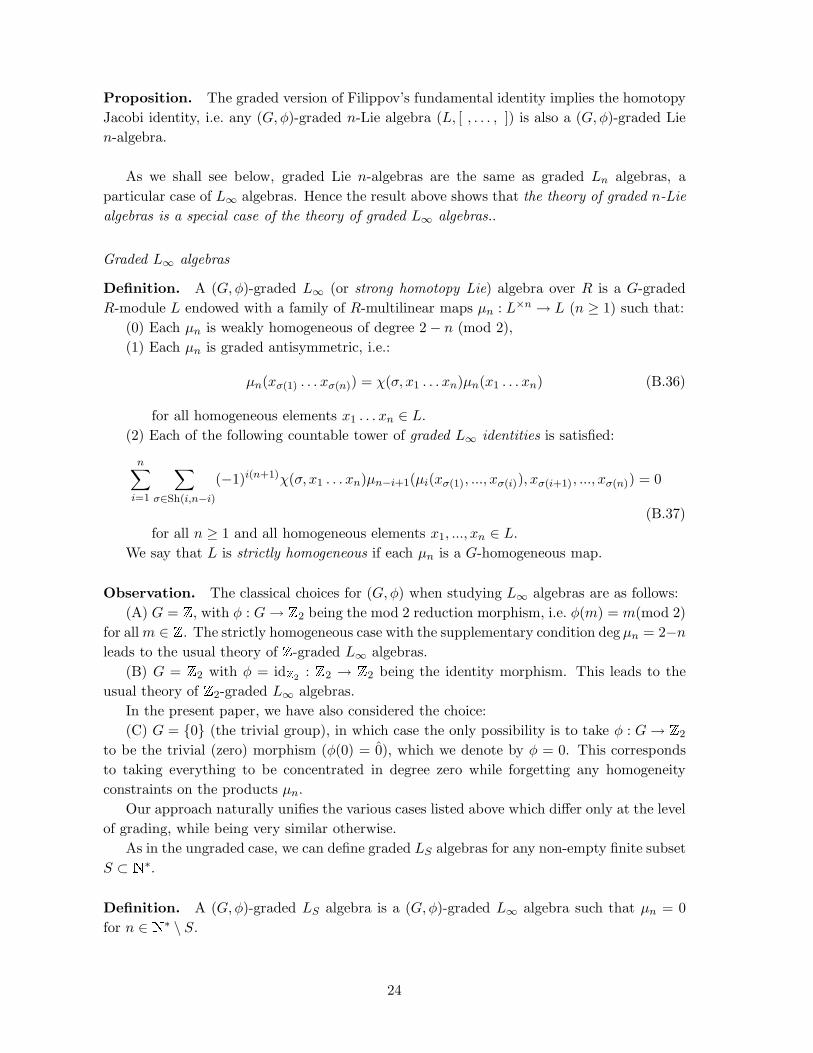
Proposition. The graded version of Filippov’s fundamental identity implies the homotopy

Jacobi identity, i.e. any (G,φ)-graded n-Lie algebra (L, [ , . . . , ]) is also a (G,φ)-graded Lie

n-algebra.

As we shall see below, graded Lie n-algebras are the same as graded Ln algebras, a

particular case of L∞ algebras. Hence the result above shows that the theory of graded n-Lie

algebras is a special case of the theory of graded L∞ algebras..

Graded L∞ algebras

Definition. A (G,φ)-graded L∞ (or strong homotopy Lie) algebra over R is a G-graded

R-module L endowed with a family of R-multilinear maps µn : L×n → L (n ≥ 1) such that:

(0) Each µn is weakly homogeneous of degree 2 − n (mod 2),

(1) Each µn is graded antisymmetric, i.e.:

µn(xσ(1) . . . xσ(n)) = χ(σ, x1 . . . xn)µn(x1 . . . xn) (B.36)

for all homogeneous elements x1 . . . xn ∈ L.

(2) Each of the following countable tower of graded L∞ identities is satisfied:

n∑

i=1

∑

σ∈Sh(i,n−i)

(−1)i(n+1)χ(σ, x1 . . . xn)µn−i+1(µi(xσ(1), ..., xσ(i)), xσ(i+1), ..., xσ(n)) = 0

(B.37)

for all n ≥ 1 and all homogeneous elements x1, ..., xn ∈ L.

We say that L is strictly homogeneous if each µn is a G-homogeneous map.

Observation. The classical choices for (G,φ) when studying L∞ algebras are as follows:

(A) G = Z, with φ : G→ Z2 being the mod 2 reduction morphism, i.e. φ(m) = m(mod 2)

for allm ∈ Z. The strictly homogeneous case with the supplementary condition deg µn = 2−nleads to the usual theory of Z-graded L∞ algebras.

(B) G = Z2 with φ = idZ2: Z2 → Z2 being the identity morphism. This leads to the

usual theory of Z2-graded L∞ algebras.

In the present paper, we have also considered the choice:

(C) G = 0 (the trivial group), in which case the only possibility is to take φ : G→ Z2

to be the trivial (zero) morphism (φ(0) = 0), which we denote by φ = 0. This corresponds

to taking everything to be concentrated in degree zero while forgetting any homogeneity

constraints on the products µn.

Our approach naturally unifies the various cases listed above which differ only at the level

of grading, while being very similar otherwise.

As in the ungraded case, we can define graded LS algebras for any non-empty finite subset

S ⊂ N∗.

Definition. A (G,φ)-graded LS algebra is a (G,φ)-graded L∞ algebra such that µn = 0

for n ∈ N∗ \ S.

24

When S = n, the corresponding LS algebras are also called graded Ln algebras. When

S = 1, . . . , n, they are called graded L(n) algebras.

Thus a (G,φ)-graded L(n) algebra has only the products µ1 . . . µn, and one needs only

consider the first 2n − 1 identities in (B.37) (those with k = 1 . . . 2n− 1) since all identities

with k ≥ 2n are satisfied trivially. An Ln algebra has only the product µn and the only

nontrivial identity in (B.37) is the one with k = 2n− 1:∑

σ∈Sh(n,n−1)

χ(σ, x1 . . . x2n−1)µn(µn(xσ(1), ..., xσ(n)), xσ(n+1), ..., xσ(2n−1)) = 0 (B.38)

for all x1, ..., x2n−1 ∈ L, which is called the graded homotopy Jacobi identity (this is also the

last nontrivial identity of an L(n) algebra). Clearly any Ln algebra is also an L(n) algebra.

Examples. (1) Consider a (G,φ)-graded L(1) algebra structure on a G-graded vector space

L. There is just one weakly homogeneous linear map µ1 of weak degree 1, and the conditions

(B.37) reduce to the single condition µ1 µ1 = 0, which says that (L,µ1) is a (G,φ)-graded

complex. Clearly a (G,φ)-graded L1 algebra is the same thing as an L(1) algebra. The choice

(A), (B) above for (G,φ) lead to the usual notions of Z-graded and Z2-graded complexes

respectively.

(2) A graded L(2) algebra has a linear unary product µ1 of weak degree 1 and a bilinear

binary product µ2, the second being graded antisymmetric and of weak degree 0. Conditions

(B.37) state that µ1 is a differential, that it is a graded derivation of µ2:

µ1(µ2(x1, x2)) = µ2(µ1(x1), x2) + (−1)x1µ2(x1, µ1(x2)) . (B.39)

and that µ2 satisfies the graded Jacobi identity:

(−1)x1x3µ2(µ2(x1, x2), x3) + (−1)x1x2µ2(µ2(x2, x3), x1) + (−1)x2x3µ2(µ2(x3, x1), x2) = 0

(B.40)

These three constraints mean that L is a differential (G,φ)-graded Lie algebra with differential

d = µ1 and graded Lie bracket [ , ] = µ2( , ). An L2 algebra is an L(2) algebra with trivial

differential, i.e. a (G,φ)-graded Lie algebra. The choices (A),(B) above for (G,φ) lead to the

usual notions of Z-graded respectively Z2-graded (differential) Lie algebras.

C. Lie n-algebras are L∞ algebras

Proposition. A Lie n-algebra over k is the same as a (G,φ)-graded Ln algebra L over k

based on choice (C) for (G,φ), i.e. G = 0 and φ(0) = 0.

Proof. Indeed, substituting this choice of (G,φ) into the definition of an Ln algebra obviously

reproduces the definition of a Lie n-algebra. It follows that Lie n-algebras are simply the

‘ungraded version’ of Ln algebras. Recall that any n-Lie algebra is a symmetric and therefore

an Lie n-algebra [31]. It follows that any n-Lie algebra is an Ln algebra. Therefore the theory

of n-Lie algebras is a special case of the theory of L∞ algebras. Thus, quite a few extensions

of the notion of a Lie algebra which have been considered in the literature are particular

cases of L∞ algebras, which, as expected from the work of Stasheff, play a unifying role.

25

References

[1] J. Bagger and N. Lambert, Gauge symmetry and supersymmetry of multiple M2-branes,

Phys. Rev. D 77 (2008) 065008 [0711.0955 [hep-th]].

[2] A. Gustavsson, Algebraic structures on parallel M2-branes, 0709.1260 [hep-th].

[3] V. T. Filippov, n-Lie algebras, Sib. Mat. Zh. 26 (1985) 126.

[4] S. Mukhi and C. Papageorgakis, M2 to D2, JHEP 05 (2008) 085 [0803.3218 [hep-th]].

[5] P.-A. Nagy, Prolongations of Lie algebras and applications, 0712.1398; G. Papadopou-

los, M2-branes, 3-Lie algebras and Plucker relations, JHEP 05 (2008) 054 [0804.2662

[hep-th]]; J. P. Gauntlett and J. B. Gutowski, Constraining maximally supersymmetric

membrane actions, 0804.3078 [hep-th].

[6] M. A. Bandres, A. E. Lipstein, and J. H. Schwarz, Ghost-free superconformal action for

multiple M2-branes, JHEP 07 (2008) 117 [0806.0054 [hep-th]].

[7] M. Van Raamsdonk, Comments on the Bagger-Lambert theory and multiple M2- branes,

JHEP 05 (2008) 105 [0803.3803 [hep-th]]; O. Aharony, O. Bergman, D. L. Jafferis,

and J. Maldacena, N=6 superconformal Chern-Simons-matter theories, M2-branes and

their gravity duals, JHEP 10 (2008) 091 [0806.1218 [hep-th]].

[8] J. Bagger and N. Lambert, Three-algebras and N=6 Chern-Simons gauge theories, Phys.

Rev. D 79 (2009) 025002 [0807.0163 [hep-th]].

[9] S. Cherkis and C. Saemann, Multiple M2-branes and generalized 3-Lie algebras, Phys.

Rev. D 78 (2008) 066019 [0807.0808 [hep-th]].

[10] P. de Medeiros, J. Figueroa-O’Farrill, E. Mendez-Escobar, and P. Ritter, On the Lie-

algebraic origin of metric 3-algebras, 0809.1086 [hep-th].

[11] S. Cherkis, V. Dotsenko, and C. Saemann, On superspace actions for multiple M2-branes,

metric 3-algebras and their classification, 0812.3127 [hep-th].

[12] T. Lada and J. Stasheff, Introduction to sh Lie algebras for physicists, Int. J. Theor.

Phys. 32 (1993) 1087 [hep-th/9209099].

[13] T. Lada and M. Markl, Strongly homotopy Lie algebras, Commun. in Algebra 23 (1995)

2147 [hep-th/9406095].

[14] S. Merkulov, L∞-algebra of an unobstructed deformation functor, Intern. Math. Research

Notices 3 (2000) 147 [0804.4555 [math.AG]].

[15] B. Zwiebach, Closed string field theory: Quantum action and the B-V master equation,

Nucl. Phys. B 390 (1993) 33 [hep-th/9206084].

26

[16] M. Alexandrov, M. Kontsevich, A. Schwartz, and O. Zaboronsky, The geometry of the

master equation and topological quantum field theory, Int. J. Mod. Phys. A 12 (1997)

1405 [hep-th/9502010].

[17] C. I. Lazaroiu, String field theory and brane superpotentials, JHEP 10 (2001) 018

[hep-th/0107162].

[18] C. I. Lazaroiu and R. Roiban, Holomorphic potentials for graded D-branes, JHEP 02

(2002) 038 [hep-th/0110288].

[19] C. I. Lazaroiu and R. Roiban, Gauge-fixing, semiclassical approximation and potentials

for graded Chern-Simons theories, JHEP 03 (2002) 022 [hep-th/0112029].

[20] C. I. Lazaroiu, D-brane categories, Int. J. Mod. Phys. A 18 (2003) 5299

[hep-th/0305095].

[21] M. Herbst, C.-I. Lazaroiu, and W. Lerche, Superpotentials, A(infinity) relations and

WDVV equations for open topological strings, JHEP 02 (2005) 071 [hep-th/0402110].

[22] C. l. Lazaroiu, On the non-commutative geometry of topological D-branes, JHEP 11

(2005) 032 [hep-th/0507222].

[23] H. Kajiura, Homotopy algebra morphism and geometry of classical string field theory,

Nucl. Phys. B 630 (2002) 361 [hep-th/0112228].

[24] R. Fulp, T. Lada, and J. Stasheff, Sh-Lie algebras induced by gauge transformations,

Commun. Math. Phys. 231 (2002) 25.

[25] M. Movshev and A. Schwarz, On maximally supersymmetric Yang-Mills theories, Nucl.

Phys. B 681 (2004) 324 [hep-th/0311132].

[26] A. M. Zeitlin, BV Yang-Mills as a homotopy Chern-Simons, 0709.1411 [hep-th].

[27] A. M. Zeitlin, Formal Maurer-Cartan structures: From CFT to classical field equations,

JHEP 12 (2007) 098 [0708.0955 [hep-th]].

[28] A. D. Popov and C. Saemann, On supertwistors, the Penrose-Ward transform and N = 4

super Yang-Mills theory, Adv. Theor. Math. Phys. 9 (2005) 931 [hep-th/0405123].

[29] A. Basu and J. A. Harvey, The M2-M5 brane system and a generalized Nahm’s equation,

Nucl. Phys. B 713 (2005) 136 [hep-th/0412310].

[30] P. Hanlon and M. Wachs, On Lie k-algebras, Advances in Mathematics 113 (1995) 206.

[31] A. S. Dzhumadil’daev, Wronskians as n-Lie multiplications, math.RA/0202043.

[32] W. Nahm, A simple formalism for the BPS monopole, Phys. Lett. B 90 (1980) 413.

[33] N. J. Hitchin, On the construction of monopoles, Commun. Math. Phys. 89 (1983) 145.

27

[34] D.-E. Diaconescu, D-branes, monopoles and Nahm equations, Nucl. Phys. B 503 (1997)

220 [hep-th/9608163].

[35] C. G. Callan and J. M. Maldacena, Brane dynamics from the Born-Infeld action, Nucl.

Phys. B 513 (1998) 198 [hep-th/9708147];

[36] P. S. Howe, N. D. Lambert, and P. C. West, The self-dual string soliton, Nucl. Phys. B

515 (1998) 203 [hep-th/9709014].

[37] N. R. Constable, R. C. Myers, and O. Tafjord, The noncommutative bion core, Phys.

Rev. D 61 (2000) 106009 [hep-th/9911136].

[38] L. Brink, J. H. Schwarz, and J. Scherk, Supersymmetric Yang-Mills theories, Nucl. Phys.

B 121 (1977) 77.

[39] J. C. Baez, Higher Yang-Mills theory, hep-th/0206130.

28