
Studies of fractional D-branes in the gauge/gravity ...
335
Studies of fractional D-branes in the gauge/gravity correspondence & Flavored Chern-Simons quivers for M2-branes Cyril Closset Facult´ e des Sciences Service de Physique Th´ eorique et Math´ ematique
-
Upload
khangminh22 -
Category
Documents
-
view
1 -
download
0
Transcript of Studies of fractional D-branes in the gauge/gravity ...
Studies of fractional D-branesin the gauge/gravity correspondence
&
Flavored Chern-Simons quiversfor M2-branes
Cyril Closset
Faculte des Sciences
Service de Physique Theorique et Mathematique

Studies of fractional D-branesin the gauge/gravity correspondence
&
Flavored Chern-Simons quiversfor M2-branes
Cyril Closset
Boursier FRIA-FNRS
These presentee en vue de l’obtention du grade de Docteur en Sciences
Faculte des SciencesService de Physique Theorique et Mathematique
Annee academique 2009-2010 Directeur de these: Riccardo Argurio

This thesis consists of two different and almost independent parts.PART ONE is based on the following two papers:
[1] R. Argurio, F. Benini, M. Bertolini, C. Closset, and S. Cremonesi,“Gauge/gravityduality and the interplay of various fractional branes” Phys. Rev. D78(2008) 046008, arXiv:0804.4470 [hep-th].
[2] F. Benini, M. Bertolini, C. Closset, and S. Cremonesi, “The N=2 cascade revis-ited and the enhancon bearings” Phys. Rev. D79 (2009) 066012, arXiv:0811.2207.[hep-th].
PART TWO is based on
[3] F. Benini, C. Closset, and S. Cremonesi,“Chiral flavors and M2-branes at toricCY4 singularities,” JHEP 02 (2010) 036, arXiv:0911.4127 [hep-th].
The following lectures notes are reproduced in the APPENDIX:
[4] C. Closset,“Toric geometry and local Calabi-Yau varieties: An introduc-tion to toric geometry (for physicists),” arXiv:0901.3695 [hep-th].
ii
Remerciements - Acknowledgments
Il y a cinq ans, je me decidai a faire mon memoire de licence en physique theorique.Par un heureux hasard, je me retrouvai sous la direction de Riccardo Argurio, pour monmemoire et ensuite pour ma these. Il m’a soutenu de bout en bout dans mon apprentissagedu metier de chercheur, toujours chaleureux et disponible. J’ai appris enormement a soncontact, et je l’en remercie grandement.
Je remercie egalement Pierre de Buyl, Francois Dehouck, Julie Delvax, Jon Demaeyer,Nathan Goldman, Ella Jamsin, Nassiba Tabti and Vincent Wens, pour tous ces repas ala cafeteria et ces trop rares midis au soleil, qui m’ont souvent fait beaucoup de bien. Unmerci particulier a Vincent et Nass pour etre toujours tellement gentils, droles et posesa la fois, vous me manquez. Un merci particulier egalement a Francois pour m’avoirsupporte dans toutes sortes de situations et pour savoir me remettre a ma place. EncoreCargese a se coltiner ensemble, mec!
Mes plus grands remerciements vont a mes proches en dehors du monde de la physique,amis et famille, qui me demontrent constamment que vivre est une entreprise bien plusriche et interessante que toutes les theories des cordes reunies. Vous savez qui vous etes.(Et vous ne lirez pas ma these, du moins je l’espere pour vous.) Morgane, merci pourtout et bien plus.
First of all, I would like to thank my collaborators: Riccardo Argurio, FrancescoBenini, Matteo Bertolini and Stefano Cremonesi. You are the best! This thesis wouldnot exist without you. It was truly great to collaborate with you, I learned a lot (actuallyalmost everything) just by talking with you guys. I thank Matteo for the great physicsexchanges, for the meeeuuuhh-thing and for always being patient and relaxed. I thankSte and Fra for our great projects together, for all these Skype exchanges and fruitfulideas and I hope we will keep working together. And thanks again Riccardo, for lettingme interrupt you with questions at whichever time of the day, for being always ready todiscuss new things, I hope this thesis convinces you that 3d theories are interesting too.And yes I will start working on gauge mediation too. ;)
I would like to thank the whole group of the Service de Physique theorique etmathematique of ULB, for the relaxed environment and the continuous stimulation itprovides. Thanks in particular to Glenn Barnich (who gave me some taste for quantumfield theory as an undergrad), Frank Ferrari and Axel Kleinschmidt for nice discussions.Thanks to Fabienne De Neyn and Marie-France Rogge for helping me out of parperworklimbo.
Among the postdocs and students, let me thank first the “old generation” of post-docs, who adopted me as one of their kind for many nights out and wild physics and
iii
non-physics discussion, even as I started my phD: Jarah Evslin (best landlord), CarloMaccaferri, Chethan Krishnan (my officemate during three years and a great friend),Stanislav Kuperstein (my conifold godfather). I also thank Emiliano Imeroni for nu-merous physics discussions, for our unfinished work on Maldacena-Nunez (a pity we gotstuck) and for letting me use his Insert Latex package. Thanks to Daniel Persson forstimulating physics discussions, fun times and great flat sharing abilities, and to AliceBernamonti for all that and more.
I thank the old and new generation of Italians and non-Italians at ULB and VUB,Francesco Bigazzi, Raphael Benichou, Neil Copland, Federico Galli, Josef Lindman Horn-lund (let’s go have a beer), Alberto Mariotti (a beer for you too), Sung-Soo Kim (greatflatmate), Semyon Klevtsov, Jakob Palmkvist, Wieland Staessens, Cedric Troessaert,Amitabh Virmani, for discussions and great parties. Thanks in particular my fellow or-ganizers of the Modave Summer school 2008 and 2009, as well as to Geoffrey Compere,Sophie de Buyl, and Stephane Detournay, and the older generation I hardly met, all ofwhom made that great experience possible. Special thanks also to the Baratin of Modave.
I also remember with gratefulness the numerous summer schools and conferences, andthe associated traveling which make the life of a physicist quite enjoyable sometimes. Inparticular, I loved the Les Houches 2007 summer school, and I would like to warmfullyacknowledge all the great people I met there. The great Trieste spring schools also deservea special mention.
Finally, I would like to thank Riccardo Argurio (again), Frederic Bourgeois, MarcHenneaux, Axel Kleinschmidt, Carlos Nunez and Alessandro Tomasiello, for accepting tobe part of my thesis jury.


Contents
1 Introduction, overview and summary 1
1.1 Motivations . . . . . . . . . . . . . . . . . . . . . . . . . . . . . . . . . . . 1
1.2 The thesis: an overview . . . . . . . . . . . . . . . . . . . . . . . . . . . . 2
1.3 Cascading RG flow and N = 2 fractional branes . . . . . . . . . . . . . . 5
1.4 Quivers for M2-branes and their generalizations . . . . . . . . . . . . . . . 6
2 Strings, branes and such 9
2.1 Elements of type II string theory . . . . . . . . . . . . . . . . . . . . . . . 9
2.1.1 D-branes . . . . . . . . . . . . . . . . . . . . . . . . . . . . . . . . 10
2.1.2 Supergravity limits and p-brane solutions . . . . . . . . . . . . . . 10
2.1.3 DBI action for the D-brane . . . . . . . . . . . . . . . . . . . . . . 12
2.1.4 Half-BPS extended objects in type II string theory; D-branes andNS5-branes . . . . . . . . . . . . . . . . . . . . . . . . . . . . . . . 13
2.2 A few words about string dualities . . . . . . . . . . . . . . . . . . . . . . 13
2.2.1 T-duality . . . . . . . . . . . . . . . . . . . . . . . . . . . . . . . . 14
2.2.2 T-duality between geometry and NS5-branes . . . . . . . . . . . . 15
2.2.3 S-duality in type IIB . . . . . . . . . . . . . . . . . . . . . . . . . . 16
2.2.4 Type IIA and M-theory . . . . . . . . . . . . . . . . . . . . . . . . 17
3 D3-branes at singularities 21
3.1 The D3-brane and N = 4 SYM: a first encounter . . . . . . . . . . . . . . 21
3.2 D-branes at singularities and quivers . . . . . . . . . . . . . . . . . . . . . 22
3.2.1 D3-branes at orbifold singularities . . . . . . . . . . . . . . . . . . 22
3.2.2 Brane fractionation at singularities . . . . . . . . . . . . . . . . . . 24
3.2.3 Closed string perspective for D3-branes on orbifolds. Supergravity 24
3.3 Branes at generic Calabi-Yau singularities . . . . . . . . . . . . . . . . . . 26
3.3.1 Homological algebra and the relation between quivers and singu-larities . . . . . . . . . . . . . . . . . . . . . . . . . . . . . . . . . . 27
3.4 Hanany-Witten setups . . . . . . . . . . . . . . . . . . . . . . . . . . . . . 28
3.5 Toric singularities and dimer models . . . . . . . . . . . . . . . . . . . . . 30
3.5.1 Toric quiver theories as dimer models . . . . . . . . . . . . . . . . 31
3.5.2 From quiver to geometry: moduli space and the forward algorithm 32
3.5.3 Kasteleyn matrix and fast forward algorithm . . . . . . . . . . . . 34
3.5.4 An example: the dP1 quiver. . . . . . . . . . . . . . . . . . . . . . 36
3.5.5 From geometry to quiver: the inverse algorithm . . . . . . . . . . . 37
v
vi Contents
I Gauge/gravity and cascades 39
4 Conformal field theories and the AdS/CFT correspondence 41
4.1 Superconformal gauge theories in 3+1 dimensions . . . . . . . . . . . . . . 41
4.1.1 N = 1 superconformal algebra . . . . . . . . . . . . . . . . . . . . 42
4.1.2 N = 4 SYM . . . . . . . . . . . . . . . . . . . . . . . . . . . . . . . 43
4.1.3 An example of an N = 2 SCFT . . . . . . . . . . . . . . . . . . . . 44
4.1.4 N = 1 SCFT: an example of a strongly coupled fixed point . . . . 44
4.2 Anti-de-Sitter space and near horizon limit . . . . . . . . . . . . . . . . . 45
4.2.1 Near horizon limit for D3-branes . . . . . . . . . . . . . . . . . . . 45
4.3 The AdS5/CFT4 correspondence . . . . . . . . . . . . . . . . . . . . . . . 46
4.3.1 Various versions of the AdS/CFT conjecture . . . . . . . . . . . . 47
4.3.2 The energy-radius relation . . . . . . . . . . . . . . . . . . . . . . . 48
4.3.3 The AdS/CFT map: general discussion . . . . . . . . . . . . . . . 48
4.3.4 The AdS5/N = 4 dictionary . . . . . . . . . . . . . . . . . . . . . . 50
4.4 From N = 4 to N = 1. Non-spherical horizons . . . . . . . . . . . . . . . 50
4.4.1 Sasaki-Einstein manifolds . . . . . . . . . . . . . . . . . . . . . . . 51
4.4.2 Conformal N = 1 toric quivers . . . . . . . . . . . . . . . . . . . . 52
4.4.3 Chiral ring of N = 1 SCFTs . . . . . . . . . . . . . . . . . . . . . . 53
4.4.4 The Klebanov-Witten theory and remarks about the AdS/CFTmap for N = 1 quivers . . . . . . . . . . . . . . . . . . . . . . . . . 54
4.5 Spontaneous breaking of scale invariance . . . . . . . . . . . . . . . . . . . 55
5 Fractional D-branes and gauge/gravity correspondence 59
5.1 Overview: the gauge gravity/correspondence . . . . . . . . . . . . . . . . 59
5.1.1 The issue of the UV completion . . . . . . . . . . . . . . . . . . . . 60
5.2 Supersymmetry conditions . . . . . . . . . . . . . . . . . . . . . . . . . . . 61
5.3 Fractional branes at the conifold singularity . . . . . . . . . . . . . . . . . 62
5.3.1 Backreacting fractional branes on the conifold: the KT solution . . 62
5.3.2 Cascade in the N = 1 quiver . . . . . . . . . . . . . . . . . . . . . 63
5.3.3 The low energy theory and the deformed conifold . . . . . . . . . . 66
5.4 Fractional branes on various singularities . . . . . . . . . . . . . . . . . . . 68
6 The N = 2 cascade revisited and the enhancon bearings 71
6.1 Introduction and overview . . . . . . . . . . . . . . . . . . . . . . . . . . . 71
6.2 D3 branes on the C2/Z2 orbifold and a cascading solution . . . . . . . . . 73
6.3 The enhancon and the Seiberg-Witten curve . . . . . . . . . . . . . . . . . 77
6.4 The cascading vacuum in field theory . . . . . . . . . . . . . . . . . . . . . 83
6.4.1 One cascade step: N = 2 SQCD . . . . . . . . . . . . . . . . . . . 84
6.4.2 The cascading vacuum in the quiver gauge theory . . . . . . . . . 85
6.4.3 The infinite cascade limit . . . . . . . . . . . . . . . . . . . . . . . 87
6.4.4 Mass deformation . . . . . . . . . . . . . . . . . . . . . . . . . . . 89
6.5 More supergravity duals: enhancon bearings . . . . . . . . . . . . . . . . . 92
6.5.1 Reconstructing the cascading vacuum at the baryonic roots . . . . 98
6.5.2 More bearings: the enhancon plasma . . . . . . . . . . . . . . . . . 99
6.6 Excisions, warp factors and the cure of repulson singularities . . . . . . . 102
Contents vii
6.7 Conclusions . . . . . . . . . . . . . . . . . . . . . . . . . . . . . . . . . . . 105
7 Cascades of mixed kind and interplay of various fractional branes 1077.1 Introduction . . . . . . . . . . . . . . . . . . . . . . . . . . . . . . . . . . . 1077.2 The orbifolded conifold . . . . . . . . . . . . . . . . . . . . . . . . . . . . . 109
7.2.1 Regular and fractional branes . . . . . . . . . . . . . . . . . . . . . 1107.2.2 Geometry, cycles and quiver ranks . . . . . . . . . . . . . . . . . . 111
7.3 Supergravity background for the UV regime . . . . . . . . . . . . . . . . . 1137.3.1 The UV regime: running fluxes and singularity lines . . . . . . . . 1137.3.2 Checks of the duality: beta functions and Maxwell charges . . . . 1167.3.3 Page charges and the RG flow from supergravity . . . . . . . . . . 121
7.4 The IR regime of the theory . . . . . . . . . . . . . . . . . . . . . . . . . . 1297.4.1 Gauge theory IR dynamics . . . . . . . . . . . . . . . . . . . . . . 1307.4.2 The Gukov-Vafa-Witten superpotential . . . . . . . . . . . . . . . 1337.4.3 IR regime and singularities resolution . . . . . . . . . . . . . . . . 136
7.5 Conclusions . . . . . . . . . . . . . . . . . . . . . . . . . . . . . . . . . . . 140
II Chern-Simons quivers and M-theory 141
8 AdS4/CFT3 and the quest for a theory of multiple M2-branes 1438.1 M2-brane solution in eleven dimensional supergravity . . . . . . . . . . . . 143
8.1.1 Energy/radius relation . . . . . . . . . . . . . . . . . . . . . . . . . 1458.1.2 Type IIA reduction . . . . . . . . . . . . . . . . . . . . . . . . . . . 145
8.2 AdS4/CFT3: the AdS side . . . . . . . . . . . . . . . . . . . . . . . . . . . 1478.3 SCFT on M2-branes? . . . . . . . . . . . . . . . . . . . . . . . . . . . . . 148
8.3.1 M2- from D2-brane: dual photon . . . . . . . . . . . . . . . . . . . 1488.3.2 Flavors and large Nf limit . . . . . . . . . . . . . . . . . . . . . . . 150
9 Superconformal theories in three dimensions 1519.1 Spinors in three dimensions and supersymmetry . . . . . . . . . . . . . . . 151
9.1.1 The parity symmetry in 2 + 1 dimensions . . . . . . . . . . . . . . 1529.1.2 Poincare algebra . . . . . . . . . . . . . . . . . . . . . . . . . . . . 1539.1.3 N -extended supersymmetry . . . . . . . . . . . . . . . . . . . . . . 154
9.2 N = 2 supersymmetry, superspace and superfields . . . . . . . . . . . . . 1559.2.1 Abelian gauge field, conserved current and N = 2 Lagrangian . . . 1579.2.2 Vector/scalar duality . . . . . . . . . . . . . . . . . . . . . . . . . . 1579.2.3 Non-abelian generalization . . . . . . . . . . . . . . . . . . . . . . 158
9.3 Chern-Simon term and topologically massive photon . . . . . . . . . . . . 1589.3.1 The pure Chern-Simons action . . . . . . . . . . . . . . . . . . . . 1589.3.2 Topologically massive gauge field . . . . . . . . . . . . . . . . . . . 159
9.4 N = 2 Chern-Simons theories . . . . . . . . . . . . . . . . . . . . . . . . . 1609.4.1 Topologically massive vector multiplet . . . . . . . . . . . . . . . . 1619.4.2 Chern-Simons-matter superconformal theories . . . . . . . . . . . . 1619.4.3 N = 2 SCFT with superpotential and weak non-renormalization
theorem . . . . . . . . . . . . . . . . . . . . . . . . . . . . . . . . . 1639.4.4 N = 3 CS-matter theory . . . . . . . . . . . . . . . . . . . . . . . . 164
viii Contents
10 Monopole operators in three dimensions 165
10.1 Monopoles in three dimensional SYM theories . . . . . . . . . . . . . . . . 166
10.1.1 The Coulomb branch . . . . . . . . . . . . . . . . . . . . . . . . . . 167
10.1.2 Monopole operator in the 3d Maxwell theory . . . . . . . . . . . . 168
10.2 Monopole operators in 3d CFT . . . . . . . . . . . . . . . . . . . . . . . . 169
10.2.1 N = 2 BPS monopole operators . . . . . . . . . . . . . . . . . . . 170
10.2.2 Induced charges from quantum effects . . . . . . . . . . . . . . . . 171
10.2.3 OPE of monopole operators . . . . . . . . . . . . . . . . . . . . . . 172
11 The ABJM theory and Chern-Simons quivers 173
11.1 The ABJM theory . . . . . . . . . . . . . . . . . . . . . . . . . . . . . . . 174
11.1.1 The ABJM moduli space . . . . . . . . . . . . . . . . . . . . . . . 176
11.2 Chiral ring and monopole operators . . . . . . . . . . . . . . . . . . . . . 177
11.2.1 Non-Abelian case . . . . . . . . . . . . . . . . . . . . . . . . . . . . 178
11.2.2 Enhanced SUSY . . . . . . . . . . . . . . . . . . . . . . . . . . . . 179
11.3 N = 2 Abelian quivers and their classical moduli space . . . . . . . . . . . 179
11.3.1 Toric Chern-Simons quivers and the Kasteleyn matrix algorithm . 182
11.4 A look at proposals for M2-brane theories . . . . . . . . . . . . . . . . . . 184
11.4.1 Brane tilings with multiple bounds . . . . . . . . . . . . . . . . . . 184
12 Chern-Simons quivers from stringy dualities 187
12.1 Fivebrane systems, M-theory/type IIB duality and ABJM . . . . . . . . . 187
12.1.1 N = 3 generalizations . . . . . . . . . . . . . . . . . . . . . . . . . 190
12.1.2 Moduli space and hyper-toric geometry . . . . . . . . . . . . . . . 191
12.2 N = 3 Flavors in ABJM: the Gaiotto-Jafferis construction . . . . . . . . . 192
12.2.1 The N0,1,0 space as an algebraic variety . . . . . . . . . . . . . . . 193
12.2.2 Recovering N0,1,0 from the quantum chiral ring . . . . . . . . . . . 194
12.3 Stringy derivation of N = 2 Chern-Simons quivers . . . . . . . . . . . . . 195
12.3.1 CY4 as a U(1) fibration . . . . . . . . . . . . . . . . . . . . . . . . 196
12.3.2 Chern-Simons quivers from type IIA . . . . . . . . . . . . . . . . . 198
13 Flavors in N = 2 toric Chern-Simons quivers 201
13.1 Motivation and overview . . . . . . . . . . . . . . . . . . . . . . . . . . . . 201
13.2 M-theory reduction and D6-branes : A top-down perspective . . . . . . . 203
13.2.1 IIA background as a CY3 fibration with D6-branes . . . . . . . . . 205
13.3 Flavoring Chern-Simons-matter theories : A bottom-up perspective . . . . 206
13.3.1 Monopole operators and flavors . . . . . . . . . . . . . . . . . . . . 208
13.4 Moduli space of flavored quivers . . . . . . . . . . . . . . . . . . . . . . . 210
13.4.1 Unflavored quivers and monopoles . . . . . . . . . . . . . . . . . . 210
13.4.2 Flavored quivers . . . . . . . . . . . . . . . . . . . . . . . . . . . . 211
13.4.3 Toric flavored CS quivers . . . . . . . . . . . . . . . . . . . . . . . 212
13.4.4 Moduli space of flavored quivers from the A-theory: a proof . . . . 213
13.5 Back to geometry: real and complex masses . . . . . . . . . . . . . . . . . 215
13.5.1 Real masses and partial resolutions . . . . . . . . . . . . . . . . . . 216
13.5.2 Complex masses . . . . . . . . . . . . . . . . . . . . . . . . . . . . 217
13.6 Examples – various flavored quiver gauge theories . . . . . . . . . . . . . . 218

Contents ix
13.6.1 Flavoring the C3 quiver . . . . . . . . . . . . . . . . . . . . . . . . 219
13.6.2 Flavoring the conifold quiver . . . . . . . . . . . . . . . . . . . . . 222
13.6.3 Flavoring the modified C× C2/Z2 theory . . . . . . . . . . . . . . 228
13.6.4 Flavoring the dP0 quiver . . . . . . . . . . . . . . . . . . . . . . . . 233
13.6.5 Flavoring the dP1 quiver . . . . . . . . . . . . . . . . . . . . . . . . 236
13.7 Conclusions . . . . . . . . . . . . . . . . . . . . . . . . . . . . . . . . . . . 237
A Type IIB SUGRA action, charges and equations of motion 239
A.1 Maxwell and Page charges for D3-branes . . . . . . . . . . . . . . . . . . . 240
B Algebraic geometry and toric geometry 241
B.1 Algebraic geometry: the gist of it . . . . . . . . . . . . . . . . . . . . . . . 241
B.1.1 Affine varieties . . . . . . . . . . . . . . . . . . . . . . . . . . . . . 242
B.1.2 Projective varieties . . . . . . . . . . . . . . . . . . . . . . . . . . . 245
B.1.3 Spectrum and scheme, in two words . . . . . . . . . . . . . . . . . 247
B.2 The Calabi-Yau condition . . . . . . . . . . . . . . . . . . . . . . . . . . . 247
B.2.1 Holomorphic vector bundles and line bundles . . . . . . . . . . . . 247
B.2.2 Calabi-Yau manifolds. Kahler and complex moduli . . . . . . . . . 248
B.2.3 Divisors and line bundles . . . . . . . . . . . . . . . . . . . . . . . 249
B.3 Toric geometry 1: The algebraic story . . . . . . . . . . . . . . . . . . . . 250
B.3.1 Cones and fan. Homogeneous coordinates . . . . . . . . . . . . . . 250
B.3.2 Coordinate rings and dual cones . . . . . . . . . . . . . . . . . . . 253
B.3.3 Calabi-Yau toric varieties . . . . . . . . . . . . . . . . . . . . . . . 256
B.3.4 Toric diagrams and p-q webs . . . . . . . . . . . . . . . . . . . . . 257
B.4 Dealing with toric singularities . . . . . . . . . . . . . . . . . . . . . . . . 258
B.4.1 Resolution of toric singularities and simplicial decomposition . . . 259
B.4.2 Deformation of toric singularities: the versal space . . . . . . . . . 261
B.5 Toric geometry 2: Gauged linear sigma-model . . . . . . . . . . . . . . . . 263
B.5.1 Kahler quotient and moment maps . . . . . . . . . . . . . . . . . . 264
B.5.2 The GLSM story . . . . . . . . . . . . . . . . . . . . . . . . . . . . 265
B.5.3 Toric varieties as torus fibration of polytopes . . . . . . . . . . . . 265
C N = 1 renormalization group and Seiberg duality 267
C.1 RG equations for N = 1 gauge theories . . . . . . . . . . . . . . . . . . . 267
C.1.1 Superpotential couplings . . . . . . . . . . . . . . . . . . . . . . . . 267
C.1.2 Gauge coupling . . . . . . . . . . . . . . . . . . . . . . . . . . . . . 268
C.2 Seiberg duality in the conformal window . . . . . . . . . . . . . . . . . . . 268
C.3 Seiberg duality with a quartic superpotential . . . . . . . . . . . . . . . . 269
D Spherical coordinates on R6 271
D.1 Spherical polar coordinates on R6 . . . . . . . . . . . . . . . . . . . . . . . 271
D.2 Spherical harmonics of S5 and Gegenbauer polynomials . . . . . . . . . . 272
D.3 Solving for the warp factor of a 2 stacks system . . . . . . . . . . . . . . . 273
x Contents
E Seiberg-Witten theory 275E.1 N = 2 vector mutliplet and the effective action . . . . . . . . . . . . . . . 275
E.1.1 R-symmetry and the perturbative prepotential . . . . . . . . . . . 277E.2 Electric-magnetic duality . . . . . . . . . . . . . . . . . . . . . . . . . . . 277E.3 Singularities and massless monopoles . . . . . . . . . . . . . . . . . . . . . 279E.4 Solution through the Seiberg-Witten curve . . . . . . . . . . . . . . . . . . 281E.5 SW curves for N = 2 SQCD with Nf flavors . . . . . . . . . . . . . . . . . 283E.6 SW curves from M-theory . . . . . . . . . . . . . . . . . . . . . . . . . . . 284E.7 Effective field theory approach to the cascading SW curve . . . . . . . . . 285
F The conifold and a Z2 orbifold thereof 287F.1 Generalities on the conifold geometry . . . . . . . . . . . . . . . . . . . . . 287F.2 The orbifolded conifold geometry . . . . . . . . . . . . . . . . . . . . . . . 289F.3 Poisson equation on the singular conifold . . . . . . . . . . . . . . . . . . 297F.4 Periods of Ω . . . . . . . . . . . . . . . . . . . . . . . . . . . . . . . . . . . 298

Chapter 1
Introduction, overview andsummary
String theory is our best candidate for a theory of gravity [5, 6] which is coherent withour quantum theoretical understanding of Physics [7, 8]. To the outsider, string theory inits present formulation(s) might look rather Baroque. Nevertheless, the student who hasspent some time amongst its wonders cannot help but suspect that string theory containssome of the deepest clues to a more comprehensive understanding of our Universe.
On a more down-to-earth tone, string theory contains the more familiar framework ofquantum field theory, which is the main tool of XXth century Physics. More surprisingly,it turns out that some quantum fields theories are equivalent to string theories. Hence,quite independently from the considerations about quantum gravity, string theory can beseen as just another tool to study interesting field theories in regimes which were hithertoout of reach.
1.1 Motivations
Our current understanding of string theory relies crucially on the concept of duality. Aduality between two theories is an exact physical equivalence, which means that anyphysical observable is the same in both theories. The two sides of the duality might ormight not look alike, depending in part on whether we are dealing with perturbative ornon-perturbative dualities.
The work of this thesis takes place in the context of the AdS/CFT correspondenceand in the more general framework known as the gauge/gravity correspondence. Thiscorrespondence is a very surprising non-perturbative duality, in which the two dual the-ories seem utterly different. The revolutionary idea behind the AdS/CFT proposal [9] isthat a quantum field theory in 3 or 4 dimensions can be dual to a gravitational theory ina higher dimensional space (10 or 11 dimensions for the best understood cases stemmingfrom string theory). This relationship is best understood when the quantum field the-ory is a conformal field theory (CFT). The dual gravity theory involves gravity, and itsultraviolet completion in the form of a string theory, in Anti-de-Sitter (AdS) space-time.
In perturbative string theory, the basic object is the fundamental string. To under-
1
2 Chapter 1. Introduction, overview and summary
stand non-perturbative dualities in string theory, it is important to study higher dimen-sional objects known as branes. Branes are the underlying theme of this work. Theyare fascinating dual objects, in the sense that they can be interpreted very differently indifferent regimes. The best understood instance of a brane is the Dirichlet brane, or D-brane. In the weakly coupled string theory, D-branes support open strings, whose degreesof freedom contain a vector field. In the case of multiple coincident D-branes, these openstring excitations possess non-Abelian gauge symmetries, similarly to the mathematicalstructure of the Standard Model. D-branes are also massive objects, which deform space-time according to the laws of General Relativity. In the appropriate supergravity limitof small space-time curvatures, they correspond to some kind of extremal black holes (orblack branes) called p-branes.
The D3-brane is particularly important. Its worldvolume spans 3+1 dimensions, sothat we could live on it. Moreover, its corresponding extremal 3-brane solution is smooth(the dilaton is constant), so that the supergravity approximation does not break down atthe horizon. These two properties make D3-branes very interesting to study. By taking anear horizon limit on D3-branes, we obtain a sting theory “derivation” of an AdS5/CFT4
correspondence. This duality has given us new tools to compute in four dimensionaltheories: one can “simply” do computations in the dual gravity background to extractobservables in a strongly coupled field theory. This makes AdS/CFT an important toolon the road to an analytic understanding of low energy QCD, which is one of the greatestproblems in theoretical physics. AdS/CFT has already been successfully used to study(at least at a qualitative level) strange properties of the quark-gluon plasma produced atRHIC. In Part One of the thesis we will study some models which have some resemblancewith zero temperature supersymmetric QCD, although we should warn the reader thatour main object of study will not be these low energy theories per se, but rather theirexotic embedding into so-called “cascading field theories”.
Another instance of AdS/CFT correspondence is the duality stemming from consider-ing the near horizon limit on M2-branes. It had been less well studied until recently, wheninteresting progress were made towards giving a Lagrangian description of the low energytheory living on multiple M2-branes. In that case, the field theory is three dimensional.The AdS/CFT correspondence could then be used as a tool to study non-perturbativeproperties of three dimensional field theories, which arise as descriptions of many con-densed matter systems. For instance, there has been a lot of activity recently in tryingto mimic high temperature superconductors from such a gravity construction. In PartTwo of the thesis, we will extend the number of examples of AdS4/CFT3 dualities whichhave an explicit string theory “derivation”.
1.2 The thesis: an overview
The work presented in this thesis takes place in the context of the gauge/gravity corre-spondence. My two main points (theses) are:
1. The supergravity solution of Bertolini et al. [10] and Polchinski [11] describingbackreacted fractional D3-branes on the C
2/Z2 orbifold has a dual field theoryinterpretation as describing a particular vacuum on the Coulomb branch of theSU(N + M) × SU(N) N = 2 quiver theory. This vacuum is the analog of the
1.2. The thesis: an overview 3
baryonic root on the Coulomb branch of N = 2 SQCD. One can also write acorrected supergravity solution which realizes explicitly the correct “ enhanconmechanism”.
2. M2-branes on any non-compact eight dimensional toric Calabi-Yau cone with com-plex codimension two singularity have a low energy field theory description in termof a Chern-Simons quiver theory coupled to flavors (fields in the fundamental repre-sentation of some gauge groups of the quiver). The field theory description cruciallyrelies on including the diagonal monopole operators (and related non-perturbativeeffects) in the discussion of the chiral ring.
These two points are carefully explained in Part One and Part Two of this thesis. Inparticular, the main arguments are contained in Chapter 6 and Chapter 13, respectively.The rest of this long text can be considered as a detailed explanation of the conceptsinvolved, necessary for the full understanding of the above two points. In the rest ofthis section we give a non-technical overview of the contents of this thesis. In the twofollowing sections we summarize our main results in more details, and we point outpossible directions for future research.
This work takes for granted some standard knowledge about four dimensional su-persymmetric field theories, and about various non-perturbative effects such as Seibergduality. We however introduce the tools we use the most in two Appendices: N = 1 su-persymmetric theories and Seiberg duality are reviewed in Appendix C, while AppendixE offers a brief account of the Seiberg-Witten approach to N = 2 supersymmetric the-ories in four dimensions. Three dimensional supersymmetric field theories, which tendto be less familiar, will be introduced thoroughly in Part Two. We have also attemptedwhenever possible to introduce all the string theory tools we use, at least at a superficiallevel.
In Chapter 2, we give a first look from above at our field of study. Our usualenvironment will be type II string theory, but we will make healthy walks into elevendimensional M-theory as well. Our main concern lies with supersymmetric branes, whichhide rich supersymmetric field theories in their bosom. In type II string theory, theseare the D-branes and the NS5-branes. Of course, in this introductory chapter we have totake a lot for granted, but the properties we will mention are common knowledge amongstring theorists of all stripe.
Chapter 3 is an important review chapter which is relevant for both Parts of thethesis. It deals with D3-branes at Calabi-Yau (CY) threefold singularities, but it shouldbe clear that the properties we discuss are valid for any D-branes (in particular for D2-branes on the same threefolds). The main point of this chapter is that all the holomorphicproperties of a given CY threefold are encoded in a so-called quiver. The quiver is aparticular field theory describing the dynamics of open strings on the D-branes, when theD-branes sit on top of the singularity. Particular focus is put on the toric case. Toricgeometry is reviewed in Appendix B.
After these preliminaries, we enter Part One, which consists of four chapters:Chapter 4 provides an introduction to the AdS/CFT correspondence, oriented to-
wards later use. We introduce the important Klebanov-Witten theory in that chapter.The discussion focuses on the case of AdS5/CFT4, which stems from the study of D3-branes, but we also make general comments which apply to the setups discussed in Part
4 Chapter 1. Introduction, overview and summary
Two of the thesis.
Chapter 5 introduces the general concept of gauge/gravity correspondence. Themotivation to consider such an extension of the duality conjecture are explained. Wefocus on one such model, called the Klebanov-Strassler model. It gives a supergravitydescription to a theory similar in many respects to N = 1 SU(N) Super-Yang-Mills infour dimensions. We will not enter into the study of the many nice properties of this model(which has become a huge field of research). Instead, we focus on a particular propertyof this model called a duality cascade. We will give a first non-technical definition of thatterm in the next section.
Chapter 6 discusses duality cascades in N = 2 supersymmetric setup. We study indetail the Coulomb branch of the quiver for D3-branes at the C×C
2/Z2 singularity, by acareful study of the associated Seiberg-Witten curve. In particular, we prove the Point 1stated earlier. That chapter is based on [2]. We also derive a whole family of supergravitysolutions corresponding to more generic Coulomb branch vacua.
Chapter 7, based on [1], considers fractional branes of various kinds on a Z2 orbifoldof the conifold. It studies from the supergravity perspective the renormalization groupflow in the dual quiver, resulting from generic brane charge assignments. This providessupport for the conjecture that the discussion of [2] also applies to generic N = 1 quivertheories corresponding to geometries with complex codimension one singularities. Wealso discuss the infrared behavior of the field theory, at the bottom of the cascade. Thisconcludes Part One.
Part Two of the thesis is concerned with M2-branes and with the related AdS4/CFT3
correspondence. It consists of six chapters.
Chapter 8 explains the general problem. There is a natural Maldacena limit wecan take on a stack of M2-branes, and consequently there should exist an AdS4/CFT3
correspondence. However, the explicit study of this correspondence had been impededfor a long time by our ignorance about the interacting CFT present at low energy on astack of coincident M2-branes. We present a panorama of this issue prior to the recentM2-brane breakthrough.
Chapter 9 introduces supersymmetric field theories in 2+1 dimensions. In partic-ular, it introduces the Chern-Simons interaction and its supersymmetric completion. Italso discusses Chern-Simons matter theories, which can give us explicit weakly coupledexamples of interacting CFTs in three dimensions.
Chapter 10 introduces monopole operators, which are of central importance to thediscussion of Chapter 13. These are local operators which create magnetic flux at a pointin Euclidian space-time. They generically play an important role in chiral ring of genericN = 2 supersymmetric CFTs, and they give rise to large non-perturbative modificationsof the moduli space of the theory.
Chapter 11 introduces the Aharony-Bergman-Jafferis-Maldacena (ABJM) theory,which is central to the recent progress in the study of CFTs for M2-branes. We focus onthe study of its moduli space and we briefly discuss the importance of monopole operatorsin that context. In the second part of the chapter we present recent proposals for N = 2theories describing M2-branes at Calabi-Yau fourfold singularities, in the form of Chern-Simons quivers. We focus on the toric case, and explain a general algorithm which allowsto find the classical moduli space of any N = 2 toric Chern-Simons quiver.

1.3. Cascading RG flow and N = 2 fractional branes 5
Chapter 12 sets to explain the correspondence between Chern-Simons quivers andM2-branes at singularities thanks to string theory/M-theory dualities. We first explainthe ABJM setup using fivebranes in type IIB, and its generalization by Tomasiello andJafferis. This leads to the interesting possibility of adding extra “flavor” fields to theABJM model, as we review, following a paper by Gaiotto and Jafferis. In the second partof the paper we review how one can derive the Chern-Simons quiver associated to anytoric Calabi-Yau fourfold, through a simple type IIA reduction. We follow a proposal byAganagic, which we slightly clarify (as already appeared in [3]).
The final Chapter 13 contains all the original results of Part Two. It is based on [3].We show that Chern-Simons quivers coupled to extra fields (flavors) naturally arise fromM2-branes at non-isolated toric CY singularities (of complex codimension two). We usetoric geometry to understand how the coupling of new flavors to a Chern-Simons quivermodifies the moduli space of the theory. We present a simple alorithm which relatesthe flavoring procedure to simple manipulations on the toric diagram, and we prove theequivalence between the geometric expectation and the non-perturbative moduli space ofthe flavored quiver. This last step uses crucially a non-perturbative chiral ring relationinvolving the monopole operators, which we conjecture to exist following similar resultsin earlier literature.
1.3 Cascading RG flow and N = 2 fractional branes
The most studied generalization of the AdS/CFT correspondence to the non-conformalrealm involves fractional D3-branes (wrapped D5-branes) at singularities. The mostcelebrated of such setups is the Klebanov-Strassler model, which considers fractionalD3-branes at the conifold singularity. Fractional branes allow to brane-engineer genericN = 1 supersymmetric field theories, which can be somewhat similar to the minimalsupersymmetric extension of the Standard Model (MSSM), and their study is thereforeof obvious interest. However, these MSSM-like theories always have some more exoticUV completion, in which the number of degrees of freedom grows continuously with theenergy. In that respect they are very different from asymptotically free theories suchas real world QCD (where the number of degrees of freedom goes to a constant in theUV). Such complicated theories are usually known as cascading quiver theories. It ispossible in principle to decouple the exotic UV completion from the phenomenologicallyinteresting IR dynamics, but not in the supergravity approximation. This squares wellwith the expectation that QCD in the large N limit can be described as a perturbativestring theory [12]. Unfortunately we would have to deal with strings on curved space,which is too hard. The next best thing we can do is to consider the supergravity limit.In that limit, the dual field theory is strongly coupled at any scale.
The main focus of Part One of the thesis is on the study of these “cascading” UVcompletions. In the gravity description, which is very well understood, the unboundedgrowth in the number of degrees of freedom is encoded in “running fluxes”: the enclosedD3-brane charge increases logarithmically with the distance (large distance means highenergy in the dual field theory). In setups which correspond to fractional D3-branes atconifold-like singularities (N = 1 fractional branes), the dual field theory interpretationof these running fluxes is well understood too: the field theory can be described bya succession of Seiberg-dual theories, with the ranks of the gauge groups continuously

6 Chapter 1. Introduction, overview and summary
increasing as we go towards the UV. For instance, the UV limit of the Klebanov-Strasslertheory is formally a SU(∞)×SU(∞) theory, quite different from the SU(M) SYM theorypresent in the IR limit.
We will study a different kind of fractional branes, known as N = 2 fractional branes.Such branes are localized at complex codimension one singularities, and they are thereforefree to move along a complex line. This corresponds to an extra Coulomb branch in thedual field theory, associated to scalar fields in the adjoint representation. The supergravitysolutions for such branes are very similar to the N = 1 case, with analogous runningfluxes1. However, the dual field theory interpretation was not clear, because there does notexist an appropriate Seiberg duality with adjoint fields. Several partial and contradictoryexplanations were present in the literature, prior to our work. In Chapter 6 we willclarify the situation by studying the simplest N = 2 example with the Seiberg-Wittentechnology. We show that the previously known supergravity solutions with runningfluxes correspond to a particular vacuum on the Coulomb branch. This vacuum is verysimilar to the so-called baryonic root inN = 2 SQCD: it is a point on the Coulomb branchwhere non-perturbative effects (instantons) break the non-Abelian part of the gauge groupfrom SU(N) to SU(Nf −N). Hence the net effect is similar to Seiberg duality, althoughthe mechanism is different. We call “the N = 2 cascade” the RG flow described bysuccessive transitions at baryonic roots. We will provide supergravity solutions for moregeneral Coulomb branch vacua. We will also explain how the Klebanov-Strassler N = 1cascade can be recovered upon mass deformation from N = 2 to N = 1, in the fieldtheory.
This complete understanding of the cascade associated with N = 2 branes allowsto consider theories where effects from both types of fractional branes are important.Particularly interesting for physical applications is the fact that generic fractional braneassignment can lead to supersymmetry breaking in the IR theory (an issue which we willnot adress in this work). In Chapter 7 we will analyze some generic cascade with mixedfeatures, and we will also comment on the supersymmetric vacua. It would be interestingto study further to the issue of SUSY breaking at the bottom of generic cascades involvinga choice of Coulomb vacuum at some steps. Another interesting (and related) directionof study would be to consider a flux compactification with a throat corresponding to aN = 2 cascade. In a purely N = 2 throat, we do not expect any metastable vacuum tobe present (and hence no possibility of a de Sitter construction like in [13]) when puttinga anti-D3 brane in the throat, because twisted flux can be transmuted into D3-branes atno cost, which would then annihilate the anti-D3-brane classically. However, in a cascadeof mixed type the situation is less clear, and there might be interesting new possibilities.
1.4 Quivers for M2-branes and their generalizations
Fifteen years after its discovery, M-theory is still very mysterious. A fundamental objectin M-theory is the M2-brane, which is the uplift of the fundamental string (and also of theD2-brane) from type IIA to M-theory. The AdS/CFT correspondence stemming from the
1Although strictly speaking we cannot use the supergravity approximation because of the singularityline, we can still consider this approximation supplemented with extra fields, corresponding to the twistedsectors of the closed string theory.
1.4. Quivers for M2-branes and their generalizations 7
near horizon limit on M2-branes was poorly understood until recently, due to the lack ofexplicit control over the CFT. The ABJM theory gave an explicit and (almost) maximallysupersymmetric Lagrangian description for the low energy theory on M2-branes, eitheron flat space or on some orbifold C
4/Zk. The ABJM theory has a weakly coupled limit atk →∞. In that limit the theory is dual to type IIA string theory on AdS4 × CP3. Thiscorrespondence is very similar to the well studied AdS5 × S5 case; many similar avenuesof research have then opened, for instance in the very active field of integrability.
This thesis is concerned with generalizations of the ABJM theory to theories withless supersymmetries. The overall aim is to understand the general relationship betweenM2-branes and the theories which describe their low energy dynamics. In particular, wewould like to know whether these new instances of the AdS/CFT correspondence canshed new light on the “intrinsic” degrees of freedom of multiple M2-branes. By intrinsic,we mean some formulation that might be considered proper to M-theory itself. We willsee in Part Two of the thesis that we give an rather pessimistic answer to that question:all the known theories which describe M2-branes are best understood as arising from adual description of M-theory, either in type IIA or type IIB string theory2. In fact, westress that the intrinsically eleven-dimensional properties of M-theories are encoded in thedual CFTs through non-perturbative effects, which go beyond the information containedin the Lagrangian. These non-perturbative effects are related to the fact that ’t Hooftoperators (monopole operators) are local in three dimensions. Further investigation ofthe monopole operators in these theories seems crucial to us. It is a complicated problemwhich goes beyond the scope of this work.
In Part Two, we will give a overview of these various issues, stressing what seemedthe most important in order to make our point. The main results will be explained inthe last chapter of the thesis. We show how M2-branes on Calabi-Yau with non-isolatedsingularities have a natural description in term of Chern-Simons quivers with flavors.
There are numerous further directions one could take to extend the results presentedhere. Some of these questions are already under investigation. One obvious question,which might also be the hardest, is how one can extend the models presented in Chapter13, which are purely Abelian, to non-Abelian quivers. The analysis of the non-Abeliancase would be very hard (indeed it is already tricky in the maximally supersymmetriccase). A crucial point, which should not be that hard to understand, is how the gaugecharges of the monopole operators are modified in the non-Abelian case: indeed thepresence of fundamental fermions should change the representation of the monopole underthe gauge group, and would be very interesting to understand how this comes about.
A further point (which is work in progress) is to carefully study the Higgs branches ofour models. In particular this is crucial to the study of N = 2 mirror symmetry betweendifferent quivers which have the same geometric branch (and the same M-theory dual).It is also important to understand how the multiple-bound brane tilings square with ourgeneral picture.
Finally, on a more hypothetical note, it would be interesting to use some of ourtheories as toy models of condensed matter systems.
2There is a class of theories, called multiple-bound brane tiling, which we do not know how to describeusing a string theory duality. More work needs to be done to clarify the status of such theories. We willdiscuss some of their problems in Part Two.


Chapter 2
Strings, branes and such
String theory is a vast subject. In this chapter, we give an patchy overlook of theframework taken for granted in the present thesis. Our main objects of study are D-branes in type II string theories. We work mainly in the supergravity limit. We also casta first look on eleven-dimensional M-theory.
2.1 Elements of type II string theory
Let us consider type II superstring theories. In the limit of weak string coupling, therelevant degrees of freedom are closed superstrings, which live in 10 dimensional space-time. In the Ramond-Neveu-Schwarz (RNS) quantization of the superstring, requiringthe absence of tachyons selects some sectors (by the GSO projection). There are twopossibilities, called type IIA and type IIB:
IIA : (NS+, NS+), (R+, NS+), (NS+, R−), (R+, R−),
IIB : (NS+, NS+), (R+, NS+), (NS+, R+), (R+, R+).
Type II theories are called such because there are two gravitinos in the spectrum (one ineach R-NS sector). In type IIA the gravitinos have opposite chiralities while in type IIBthey have the same chirality (say positive). Hence type IIA string theory is non-chiralwhile type IIB is chiral.
Note also that the massless modes in the RR sector fill up a bispinor, which decom-poses into various anti-symmetric tensors:
IIA : 8+ ⊗ 8− = 8v + 56v,
IIB : 8+ ⊗ 8+ = 1+ 28+ 35sd
In type IIA we have a vector and a 3-form, while in type IIB we have a scalar, a 2-form anda 4-form with self-dual field strength. Moreover, the space-time theory is supersymmetric[14].
9
10 Chapter 2. Strings, branes and such
2.1.1 D-branes
In perturbative string theory, D-branes are defined as hypersurfaces on which open stringscan end. Instead of Neumann boundary conditions na∂aX
µ = 0, one can specify Dirichletboundary conditions
XµD = cst
along some 9−p directions µD = p+1, · · · , 9, at the cost of breaking translation invariancein space-time. The Dp-brane is the (p + 1)-dimensional hypersurface defined by theseboundary conditions. Moreover, one can see already at the perturbative level that Dp-branes must be dynamical objects. The quantization of the open string on the Dp-branegives, at the massless level, a p+1 dimensional vector field, 9−p scalars, and the additionalfermions required by sypersymmetry. The scalars correspond to the fluctuations of theD-brane in the 9 − p transverse directions. From the space-time perspective they areinterpreted as Goldstone bosons for the translation invariance spontaneously broken bythe D-brane.
Indeed, the non-perturbative point of view is that D-branes are solitonic states ofthe type II theories. In that sense they are fully dynamical objects, albeit very heavy inthe perturbative string limit. We are particularly interested in D-branes which preservesome supersymmetries. A stack of parallel Dp-branes of a single type preserve half ofthe supersymmetries [15], namely Q + Γp+1···9Q. Such BPS states are stable and carryconserved charges, which appear as central charges in the 10 dimensional super-Poicarealgebra [16, 14]. For a Dp-brane it appears as
Qα, ˜Qβ = −2τp ZRµ1···µp (Γµ1 · · ·Γµp)αβ (2.1)
in the commutator of two supercharges of opposite chirality in 10 dimensions. Since thecharges ZRµ1···µp carry Lorentz indices along the Dp-brane spatial directions, they are notcentral charges in the usual sense, but indeed this is because extended objects breakrotational invariance. If we dimensionally reduce along the D-brane volume they becomeusual central charges associated to a charged particle in 10−p dimensions. The Dp-branetension is
τp =1
(2π)pα′ p+12 gs
, (2.2)
where gs is the closed string coupling constant. Usualy solitons have a tension whichscales as 1/g2; D-branes are not real solitons of the closed string theory in that sense,but should rather be seen as additional fundamental objects in type II string theory.
A fundamental property of D-branes is that they carry non-Abelian gauge fields. Inperturbative string theory this follows from the well-known argument using Chan-Patonfactors [17, 18]: oriented open strings on a stack of N D-branes naturally carry U(N)degrees of freedom. Many gauge field theories can be engineered using D-branes.
2.1.2 Supergravity limits and p-brane solutions
The low energy limit of type IIA/B string theory is type IIA/B supergravity. In this thesiswe will mostly be concerned with the bosonic fields, so we write the bosonic actions only.

2.1. Elements of type II string theory 11
Common to both type IIA and type IIB is the low energy theory for the NS-NS sector,namely for the metric, the B-field and the dilaton. In Einstein frame, the action reads
SNS =1
2κ2
∫
d10x√−GR − 1
4κ2
∫[dΦ ∧ ∗dΦ+ e−ΦH3 ∧ ∗H3
](2.3)
where2κ2 = (2π)7α′4g2s (2.4)
is basically the Newton coupling constant. The Einstein frame is defined from the stringframe by rescaling the metric by the fluctuating part of the dilaton field, while its VEVeΦ0 = gs has been absorbed into κ. Φ is then the fluctuating part of the dilaton. H3 = dB2
is the NS-NS field strength. The full IIA bosonic action also contains kinetic terms forthe RR potentials as well as various interactions, including a Chern-Simon term. Let usdefine the improved field strength for a p-form potential,
Fp+1 = dCp + Cp−3 ∧H3 . (2.5)
The bosonic IIA action is
SIIA = SNS −1
4κ2
∫ [
e3Φ2 F2 ∧ ∗F2 + e
Φ2 F4 ∧ ∗F4 +B2 ∧ F4 ∧ F4
]
. (2.6)
The equations of motion are easily derived. We will not write them here because we willnot really need them in this work.
The type IIB supergravity action is a bit more tricky, because we have to make surethat the field strength F5 is self-dual. We can write the following action,
SIIB = SNS −1
4κ2
∫ [
e2ΦF1 ∧ ∗F1 + eΦF3 ∧ ∗F3 +1
2F5 ∧ ∗F5 − C4 ∧H3 ∧ F3
]
(2.7)but we have to supplement the equations of motion with the self-duality condition F5 =∗F5
1. We review the type IIB equations of motions in Appendix A.There exist an interesting class of solutions to type IIA/B SUGRA which where found
by Horowitz and Strominger [20]. They are called black p-branes, and are a generalizationof the Reissner-Nordstrom black hole to 10 dimensions. We will only be concerned withthe extremal solutions, which are half-BPS. They are most easily written in string frame.Consider the action
S =1
2κ2
∫
d10x√
−Gs(
e−2ΦR+ e−2Φ4∂µΦ∂µΦ− 1
2|Fp+2|2
)
, (2.8)
with H3 = 0. The extremal p-brane metric reads
ds2s = H− 12 ηµνdx
µdxν +H12 δijdy
idyj , (2.9)
with µ = 0, · · · p, i = p+ 1, · · · , 9, and the H is any harmonic function in the transversedirections,
∆yH = 0 . (2.10)
1Note however that a formalism to write an action for a self-dual form has been developed in [19].

12 Chapter 2. Strings, branes and such
The dilaton and the RR gauge field are given by
eΦ = gsH(3−p)
4 , gsCp+1 = H−1dx0 ∧ · · · ∧ dxp . (2.11)
This is also a solution for p = 3, although the case of a 3-brane is more subtle since it isboth an electric and a magnetic source for C4. A typical form for the warping functionH is
H(y) = 1 +n∑
i=1
(Li
|y − yi|
)7−p
. (2.12)
It corresponds to a multi-centered solution. We can interpret it as the gravity solutiondescribing n stacks of Dp-branes, each stack carrying charge Ni. More precisely,
L7−pi = Ni
2κ2 τp(7− p)Vol(S8−p)
= Ni(2π√α′)7−p
(7− p)Vol(S8−p)gs . (2.13)
This second expression is valid in Einstein frame, in which case the brane tension τpis the one in (2.2). As expected for a BPS solution, we can superpose solutions at nocost in energy. One can also see from a probe brane analysis that for a Dp-brane thegravitational attraction is exactly canceled by the repulsion from the RR potential.
2.1.3 DBI action for the D-brane
A fundamental property of D-branes in type II string theory is that, as implied by theidentification of the last subsection, they are charged under the RR fields. The centralcharge appearing in (2.1) can always be understood as related to the gauge potentialcoupling electrically to the extended object. In the case of a D-brane,
Zµ1···µp ∼∫
d9−px (∗d ∗ dCp)0µ1···µp , (2.14)
where one integrates over the 9 − p spatial directions transverse to the D-brane. Theusual coupling of a vector potential to a point particle generalizes to
SWZ = τp
∫
p+1Cp . (2.15)
We can also write an action describing the classical dynamics of a D-brane, similar to theNambu-Goto action for the string. This low energy action also involves the B-field andthe U(1) vector field living on the D-brane. It can be determined, for instance, by askingfor consistency with the various string dualities (to be discussed below). It is called theDirac-Born-Infeld (DBI) action, being a supersymmetric generalization of the Born-Infeldaction [21]. Its bosonic part is
SDBI = −τp∫
Dpdp+1ξ
√
− det(Gs +B2 + 2πα′F2) (2.16)
Here F2 = dA is the worldvolume field strength, and the background metric Gs and B-field B2 are pulled-back quantities. The total bosonic action is the sum S = SWZ+SDBI .In this thesis we will rather work with the Einstein frame expression, which is given inAppendix A.
2.2. A few words about string dualities 13
2.1.4 Half-BPS extended objects in type II string theory; D-branes andNS5-branes
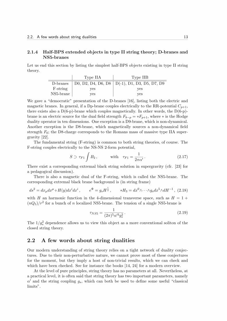
Let us end this section by listing the simplest half-BPS objects existing in type II stringtheory.
Type IIA Type IIB
D-branes D0, D2, D4, D6, D8 D(-1), D1, D3, D5, D7, D9F-string yes yes
NS5-brane yes yes
We gave a “democratic” presentation of the D-branes [16], listing both the electric andmagnetic branes. In general, if a Dp-brane couples electrically to the RR-potential Cp+1,there exists also a D(6-p)-brane which couples magnetically. In other words, the D(6-p)-brane is an electric source for the dual field strength F8−p = ∗Fp+1, where ∗ is the Hodgeduality operator in ten dimensions. One exception is a D9-brane, which is non-dynamical.Another exception is the D8-brane, which magnetically sources a non-dynamical fieldstrength F0; the D8-charge corresponds to the Romans mass of massive type IIA super-gravity [22].
The fundamental string (F-string) is common to both string theories, of course. TheF-string couples electrically to the NS-NS 2-form potential,
S ⊃ τF1
∫
B2 , with τF1 =1
2πα′. (2.17)
There exist a corresponding extremal black string solution in supergravity (cfr. [23] fora pedagogical discussion).
There is also a magnetic dual of the F-string, which is called the NS5-brane. Thecorresponding extremal black brane background is (in string frame)
ds2 = dxµdxµ+H(y)dxidxi , eΦ = gsH
12 , ∗H3 = dx0∧· · ·∧gsdx5∧dH−1 , (2.18)
with H an harmonic function in the 4-dimensional transverse space, such as H = 1 +(nQ5)/r
2 for a bunch of n localized NS5-brane. The tension of a single NS5-brane is
τNS5 =1
(2π)5α′3g2s. (2.19)
The 1/g2s dependence allows us to view this object as a more conventional soliton of theclosed string theory.
2.2 A few words about string dualities
Our modern understanding of string theory relies on a tight network of duality conjec-tures. Due to their non-perturbative nature, we cannot prove most of these conjecturesfor the moment, but they imply a host of non-trivial results, which we can check andwhich have been checked. See for instance the books [14, 24] for a modern overview.
At the level of pure principles, string theory has no parameters at all. Nevertheless, ata practical level, it is often said that string theory has two important parameters, namelyα′ and the string coupling gs, which can both be used to define some useful “classicallimits”.

14 Chapter 2. Strings, branes and such
• gs is the string coupling, which measure the tendency of strings to split. The gsexpansion is an expansion in string loops. This expansion is very similar to theperturbative expansion of quantum field theories. It gives the S-matrix elements interm of the genus expansion of the string worldsheet. gs = 0 is the classical stringlimit. It is well known that gs is itself determined by the background value of thedilaton field, gs = eΦ.
• The α′ expansion is an expansion around the point particle limit; the length scale√α′ = ls is called the string length. The proper expansion parameter to consider
is a dimensionless parameter such as α′p2, where p2 is the characteristic scale ofinterest. ls sets the mass of the massive string states, which are necessary for thespectacular UV finiteness of string theory. It can be taken as a unit of length instead of the 10 dimensional Planck length κ
14 (see the relation (2.4)). In the low
energy limit p2 ≪ 1/α′ we obtain an effective theory of massless particles in theguise of a non-renormalizable supergravity theory.
Let us go for a brief review of string theory dualities.
2.2.1 T-duality
Historically the oldest, T-duality is a perturbative duality, which holds order by order inthe gs expansion. We refer to [25] for a comprehensive review. The simplest example ofT-duality is for string theory on R
8,1 × S1, with S1 a circle of radius R. The momentumalong the periodic direction is quantized as n/R, n ∈ Z. In the case of a string, thereis also a conserved winding number w. T-duality states that any physical observable(spectrum and scattering amplitudes) is invariant under the exchange
n ↔ w R ↔ α′
R. (2.20)
Momentum is exchanged with winding number, and a circle of radius R becomes a circleof radius α′/R. This duality famously lead to the discovery of D-branes: suppose we haveopen strings in 10 dimensions. The winding number of an open string is not conserved.In the T-dual picture, the momentum along S1 should not be conserved either: we have aD8-brane, which breaks translational invariance. One can show explicitly that T-dualityexchanges Neumann and Dirichlet boundary conditions for open strings [18].
We can perform T-duality on much more general backgrounds. T-duality relatestwo different backgrounds (the string target space) which are indistinguishable from thepoint of view of string theory, because the world sheet theory (or more precisely thePolyakov path integral) is invariant under the background field transformation. In typeII superstring theory, T-duality exchanges type IIA and type IIB. In the presence ofclosed strings only, the change in the background is encoded in the Buscher’s rules [26].T-duality mixes together B-field and metric, and relates the string couplings as
gs ↔√α′
Rgs . (2.21)
Consistently, the Busher rules transformation for the NS-NS fields are symmetries of thesupergravity equations. The RR gauge potentials change as (schematically)
Cp+1 ↔ Cp or Cp+2 , (2.22)

2.2. A few words about string dualities 15
according to whether Cp has or does not have a leg along the direction we T-dualizealong. D-branes are T-dualized accordingly,
Dp-brane ↔ D(p− 1)-brane or D(p+ 1)-brane . (2.23)
2.2.2 T-duality between geometry and NS5-branes
For completeness, we should also discuss how T-duality acts on NS5-branes. That dependson the direction along which we T-dualize. If we T-dualize along the worldvolume of theNS5-brane, T-duality merely maps the type IIA NS5-brane to the type IIB NS5-brane.Things become more interesting when we want to T-dualize along a transverse direction.Because the B-field and the metric mix under T-duality, an NS5-brane can map to puregeometry [27, 28].
Let us consider the problem from the point of view of some geometry. The idea is toT-dualise along some S1 fiber of the geometry. At points where the S1 fiber shrinks tozero, there is a corresponding singularity in the T-dual B-field, which is interpreted as aNS5-brane source.
Let us work out part of the story at the level of supergravity, although the full storyis more involved [27, 28]. We consider the simple case of the ALE (asymptotically locallyeuclidian) metric on the singularity C
2/Zn, with coordinates
z1 = rei(φ2+ ψ
2n) cos
θ
2, z2 = rei(
φ2− ψ
2n) sin
θ
2. (2.24)
The range of φ and ψ is [0, 2π) and [0, 4π), respectively. The flat metric is simply a Hopffibration,
ds24 = dz1dz1 + dz2dz2 = dr2 +r2
4
(
dθ2 + sin2 θdφ2 +1
n2(dψ + n cos θdφ)2
)
. (2.25)
Considering this as a background of type IIA/B, we can T-dualize to type IIB/A in thesupergravity limit, along the ψ direction, by using Buscher’s rules [26] 2. The T-dualfields are
ˆds24 = dr2 +r2
4(dθ2 + sin2 θdφ2) +
4n2
r2dψ2 , (2.26)
e2(Φ−Φ0) =4n2
r2, B = n cos θ dφ ∧ dψ. (2.27)
The linear dilaton profile and the H3 = dB flux should correspond to n NS5-branes.Indeed we have the magnetic charge
1
16π2
∫
S3
H3 = n. (2.28)
2In this case the Buscher rules tell us that
Gψψ =1
Gψψ, e2Φ =
e2Φ
Gψψ, Gµν = Gµν − GµψGνψ
Gψψ, Bµψ =
GµψGψψ
,
where G is the string frame metric, and µ,ν are any coordinate index different from ψ.
16 Chapter 2. Strings, branes and such
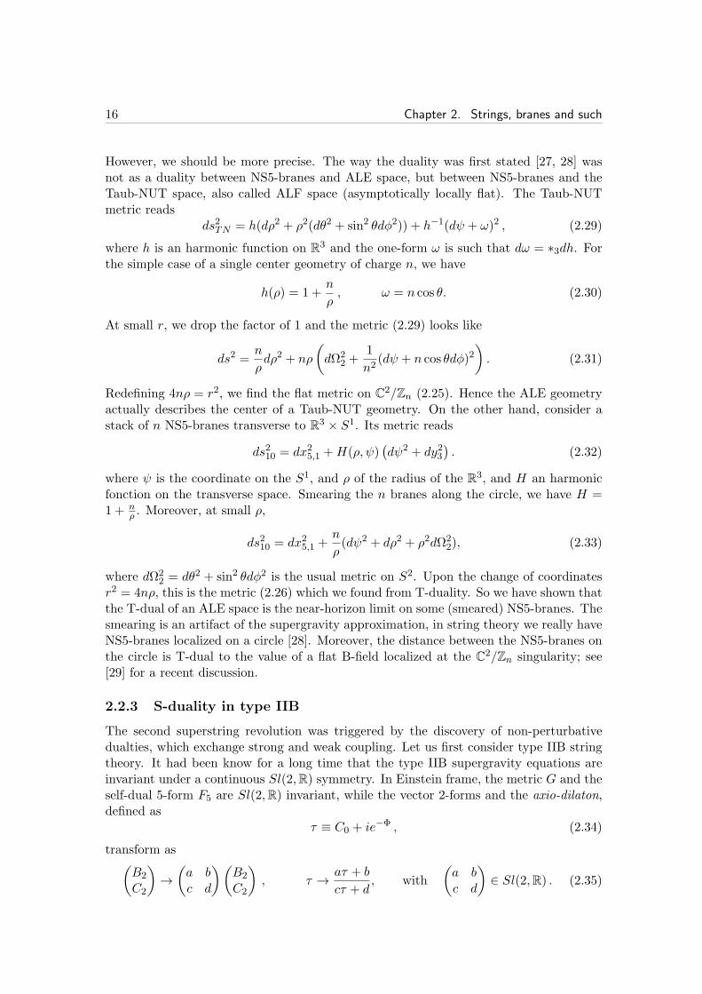
However, we should be more precise. The way the duality was first stated [27, 28] wasnot as a duality between NS5-branes and ALE space, but between NS5-branes and theTaub-NUT space, also called ALF space (asymptotically locally flat). The Taub-NUTmetric reads
ds2TN = h(dρ2 + ρ2(dθ2 + sin2 θdφ2)) + h−1(dψ + ω)2 , (2.29)
where h is an harmonic function on R3 and the one-form ω is such that dω = ∗3dh. For
the simple case of a single center geometry of charge n, we have
h(ρ) = 1 +n
ρ, ω = n cos θ. (2.30)
At small r, we drop the factor of 1 and the metric (2.29) looks like
ds2 =n
ρdρ2 + nρ
(
dΩ22 +
1
n2(dψ + n cos θdφ)2
)
. (2.31)
Redefining 4nρ = r2, we find the flat metric on C2/Zn (2.25). Hence the ALE geometry
actually describes the center of a Taub-NUT geometry. On the other hand, consider astack of n NS5-branes transverse to R
3 × S1. Its metric reads
ds210 = dx25,1 +H(ρ, ψ)(dψ2 + dy23
). (2.32)
where ψ is the coordinate on the S1, and ρ of the radius of the R3, and H an harmonic
fonction on the transverse space. Smearing the n branes along the circle, we have H =1 + n
ρ . Moreover, at small ρ,
ds210 = dx25,1 +n
ρ(dψ2 + dρ2 + ρ2dΩ2
2), (2.33)
where dΩ22 = dθ2 + sin2 θdφ2 is the usual metric on S2. Upon the change of coordinates
r2 = 4nρ, this is the metric (2.26) which we found from T-duality. So we have shown thatthe T-dual of an ALE space is the near-horizon limit on some (smeared) NS5-branes. Thesmearing is an artifact of the supergravity approximation, in string theory we really haveNS5-branes localized on a circle [28]. Moreover, the distance between the NS5-branes onthe circle is T-dual to the value of a flat B-field localized at the C
2/Zn singularity; see[29] for a recent discussion.
2.2.3 S-duality in type IIB
The second superstring revolution was triggered by the discovery of non-perturbativedualties, which exchange strong and weak coupling. Let us first consider type IIB stringtheory. It had been know for a long time that the type IIB supergravity equations areinvariant under a continuous Sl(2,R) symmetry. In Einstein frame, the metric G and theself-dual 5-form F5 are Sl(2,R) invariant, while the vector 2-forms and the axio-dilaton,defined as
τ ≡ C0 + ie−Φ , (2.34)
transform as(B2
C2
)
→(a bc d
)(B2
C2
)
, τ → aτ + b
cτ + d, with
(a bc d
)
∈ Sl(2,R) . (2.35)
2.2. A few words about string dualities 17
In the quantum theory (type IIB string theory), this symmetry cannot hold, because itwould contradict the Dirac quantization of charge. Nevertheless, it is possible that thefull type IIB string theory is invariant under the S-duality group Sl(2,Z). In particular,the so-called S generator of Sl(2,Z) acts as
τ → −1
τ. (2.36)
For C0 = 0, this transformation sends the string coupling gs to 1/gs3. This conjecture
gives us a way to deal with type IIB string theory at strong coupling: we just have toconsider the weakly coupled S-dual version of type IIB! Under S-duality, the F1-string ismapped to the D1-string, and the NS5-brane is mapped to the D5-brane. This is possiblesince, when C0 = 0,
τF1 = gsτD1 τNS5 =1
gsτD5 . (2.37)
We also have more general (p, q)-strings and (p, q)-branes, with p being the NS-NS chargeand q the RR charge. (p, q) objects with p and q coprime are all in the same Sl(2,Z)orbit as (1, 0). Each type of string gives a possible starting point for string perturbationtheory, so that type IIB string theory has an infinite family of semi-classical limits.
2.2.4 Type IIA and M-theory
A natural question to ask is whether there is something similar to S-duality for the typeIIA superstring. Type IIA supergravity has no similar S-duality, but another fact aboutsupergravities turns out to be crucial.
In eleven dimension one can write a unique supergravity theory [30]. It contains ametric G11, a gravitino and a 3-form gauge field A3, with field strength G4 = dA3. Thebosonic part of the action is quite simple, consisting of a kinetic term and of a Chern-Simons term,
S =1
2κ211
∫
d11x√
−G11
(
R− 1
2|G4|2
)
− 1
12κ211
∫
A3 ∧G4 ∧G4 . (2.38)
It is useful to define an eleven dimensional Planck length lp by
(2π)8l9p = 2κ211 . (2.39)
To make contact with string theory, we should make the link with a 10 dimensionaltheory. This can be done by a Kaluza-Klein reduction. It is well known (see for instance[31, 32]) that the reduction of Einstein theory in D dimension along a circle leads to atheory for a D − 1 dimensional metric together with a U(1) vector and a dilaton scalarfield, which parametrizes the size of the circle. We must also reduce the three form A3,which gives both a 2-form and a 3-form in 10 dimensions. In total we have the bosoniccontent of type IIA supergravity, and the details (including the fermions) can be workedout too. At the end of the day the dimensional reduction of 11 dimensional supergravityprecisely gives type IIA supergravity (2.6). The bosonic part of the story is easy to workout, and more details will be given in Chapter 8.
3We refer to the Appendix E for a discussion of a similar S-duality in the field theory context.
18 Chapter 2. Strings, branes and such
Type IIA supergravity is a consistent truncation of 11 dimensional supergravity, whichmeans that any solution of the type IIA equations of motion will be a solution of the 11dimensional theory, but not the other way around. The full eleven-dimensional theorycan be accounted for by keeping the towers of Kaluza-Klein (KK) modes.
Such KK modes have masses m = n/R10, with n ∈ Z and R10 the radius of the circlealong which we compactify. The claim is that the KK modes corresponding to a gravitonalong the circle (together with its supersymmetric partners) precisely corresponds tothe D0-brane of type IIA string theory. Since the mass of a D0-brane is 1/
√α′gs, this
identification is possible only ifR10 =
√α′gs. (2.40)
According to this relation, at strong coupling gs → ∞ the eleventh dimension becomeslarge and essentially decompactifies. In general, the radius of the eleventh dimensionmight vary in space, in which case there is a non-trivial dilaton profile in type IIA. Wealso have the important relation
lp =√α′g
13s . (2.41)
While lp and ls =√α′ provide natural units of lenght in 11 and 10 dimensions, respec-
tively, we see that the conversion factor is given by g1/3s .
The conjecture is that type IIA at strong coupling is described by a eleven-dimensionalquantum theory called M-theory, and that there is a duality at any coupling between typeIIA and M-theory [33, 34, 35]. We usually call the circle of the eleventh direction theM-theory circle.
We do not know much about M-theory. What we know is that its low energy limit is11 dimensional supergravity. We also know that it contains half-BPS extended objectsof dimension 2 + 1 and 5 + 1, called M2- and M5-branes. Their tensions are
τM2 =1
(2π)2 l3p, τM5 =
1
(2π)5 l6p. (2.42)
Using the relation (2.41), we see that the M2-brane tension is the same as the D2-branetension. We will then identify these two objects: if the M-theory circle is transverse tothe M2-brane, we obtain a D2-brane [36]. On the other hand, if the M-theory circle liesalong the M2-brane worldvolume, the reduction will give a fundamental string [37], withthe correct tension
τF1 = 2πR10τM2 =1
2πα′. (2.43)
Similarly we may identify the M5-brane with the type IIA NS5-brane when the circleis transverse, or with a D4-brane when the circle is parallel. Indeed τNS5 = τM5 andτD4 = 2πR10τM5.
Finally, we should discuss the case of D6-branes. They couple magnetically to C1.Hence their M-theory lift should be the “magnetic dual” of gravitons along the M-theorycircle: the M-theory uplift of a D6-brane is a Taub-NUT space, also called KK monopole.In a KK monopole the M-theory circle S1 is non-trivially fibered over R3. While the totalspace is topologically R
4, the metric asymptotes to S1 × S2 at infinity in R3. In the case
of n D6-branes, the first Chern class of the S1 fibration is n, and the resulting Taub-NUTof charge n is topologically R
4/Zn.We can summarize the type IIA/M-theory duality in the following table:
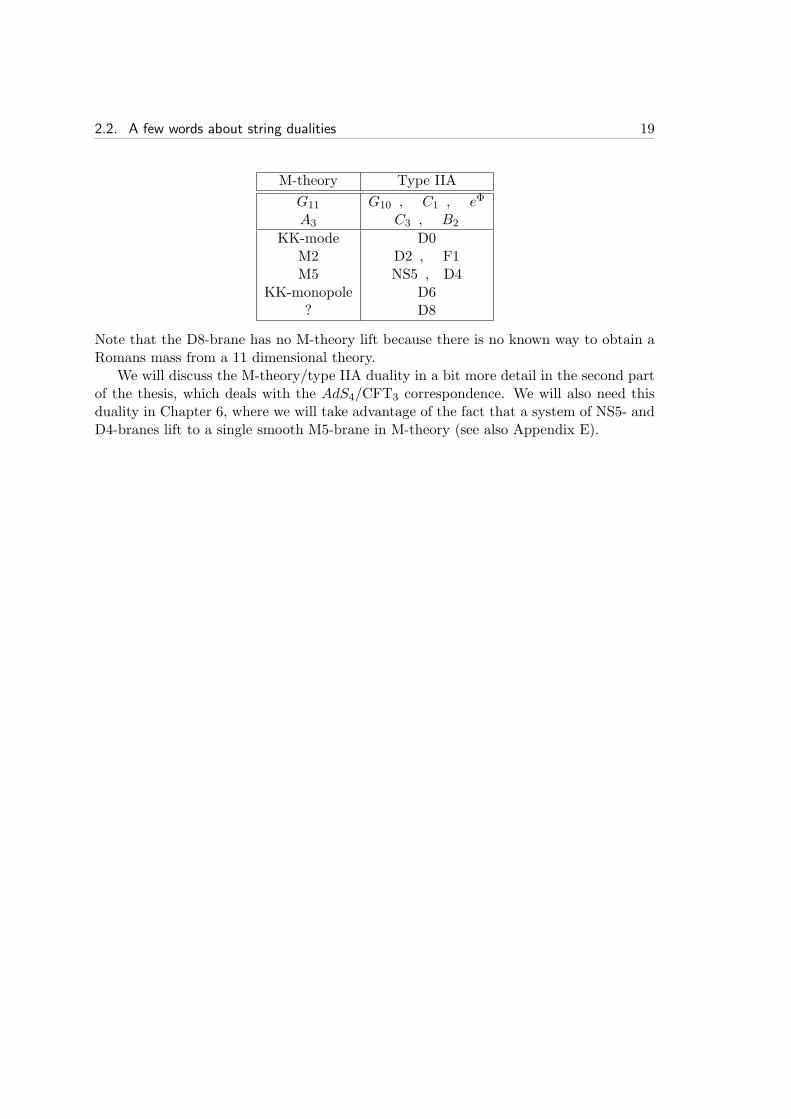
2.2. A few words about string dualities 19
M-theory Type IIA
G11 G10 , C1 , eΦ
A3 C3 , B2
KK-mode D0M2 D2 , F1M5 NS5 , D4
KK-monopole D6? D8
Note that the D8-brane has no M-theory lift because there is no known way to obtain aRomans mass from a 11 dimensional theory.
We will discuss the M-theory/type IIA duality in a bit more detail in the second partof the thesis, which deals with the AdS4/CFT3 correspondence. We will also need thisduality in Chapter 6, where we will take advantage of the fact that a system of NS5- andD4-branes lift to a single smooth M5-brane in M-theory (see also Appendix E).

Chapter 3
D3-branes at singularities
In this Chapter we review the deep relationship which exists between D-branes at sin-gularities and quiver gauge theories. The tools we introduce will be put to good use atvarious points in this thesis.
In section 3.1 we make our first encounter with N = 4 super-Yang-Mills. In section3.2, we explain how to find the field theory living on a stack of D3-branes at any flatorbifold singularity, which leads us to introduce quivers. In section 3.3 we briefly discussthe general case, for any Calabi-Yau singularity. In section 3.4 we introduce a simpleHanany-Witten brane construction, which is interesting to deal with a simple class ofconifold singularities. In section 3.5 we consider the case of a general toric CY singularity,and explain what are brane tilings and why they are useful.
3.1 The D3-brane and N = 4 SYM: a first encounter
D3-branes are special among the the zoo of Dp-branes. For instance, the p-brane metricis singular at r = 0 unless p = 3 [38]. Importantly, the extremal 3-brane solution (2.9)-(2.11) has constant dilaton, eΦ = gs. In the open string picture, this corresponds to thefact that the Yang-Mills coupling, which appears in the action as
SYM = − 1
4g2YM
∫
d4xTrFµνFµν , (3.1)
is classically marginal in four dimensions. We have the relation g2YM = 4πg2o = 4πgs,where go is the open string coupling. It turns out that the quantum theory living ona stack of N D3-brane is a maximally supersymmetric U(N) gauge theory which hasan exactly marginal coupling gYM . It is called N = 4 super-Yang-Mills (SYM), and itcontains a single N = 4 multiplet in the adjoint of U(N). In term of N = 1 superfields,the N = 4 multiplet splits into a vector multiplet V and three chiral multiplets Φi,i = 1, 2, 3. The chiral multiplets correspond to excitations along the three complexdirections zi transverse to the D3-brane. One has the relation Φi = 2πzi/α
′ betweenthe VEVs of the scalar component of the chiral superfields and the positions zi of theD3-branes. The N = 4 theory written in N = 1 form also has a superpotential
W = Φ1[Φ2,Φ3] , (3.2)
21

22 Chapter 3. D3-branes at singularities
with a precise value for the coupling dictated by the extended supersymmetry. This isall we need to know about N = 4 SYM for the moment.
3.2 D-branes at singularities and quivers
D-branes are interesting probes for singularities in string theory, because they can probea geometry which is more local than the string length
√α′. This is obviously the case for
a D0-brane, for instance, which is a point particle. Another possibility is to consider aD3-brane in R
3,1 × CY3, which is a point particle from the Calabi-Yau perspective. Wewant to know what happens to such a D3-brane probe when it goes to a singularity inthe CY3.
We consider only algebraic singularities. Actually, we consider only Calabi-Yau singu-larities, so that there is still at least N = 1 supersymmetry on the D3-brane worldvolume.An introduction to the relevant concepts of algebraic geometry, with particular focus ontoric geometry, is provided in Appendix B.
The simplest local Calabi-Yau 3-fold to consider is C3, which is just flat space. If weput a D3-brane on flat space, the low energy theory on its worldvolume is the N = 4SYM theory, as we just reviewed.
3.2.1 D3-branes at orbifold singularities
The simplest local algebraic singularity we can think of is an orbifold of flat space, C3/Γ,for Γ a discrete group. The low energy theory on probe D3-branes at the singularity wasfound in [39, 40]. The action of Γ should preserve the Calabi-Yau condition, which isequivalent to say that it preserves the Kahler and the homolomorphic forms,
J = −i3∑
i=1
dzi ∧ dzi, Ω = dz1 ∧ dz2 ∧ dz3 . (3.3)
To preserve J , Γ we must preserve the norm∑
i |zi|2 in C3, while to preserve Ω it must
be of unit determinant. Hence Γ must be a discrete subgroup of SU(3). We denote theΓ action by
g ∈ Γ : zi 7→ ρ(g)ijzj , (3.4)
where ρ(Γ) is some representation of Γ that we have to choose. We can understand thetheory on a stack of N D3-brane by working on the covering space of C3/Γ, which isjust C
3. There we have |Γ| = dimΓ images for each D3-brane. The theory for N D3-branes on the orbifold is then some projection of the U(|Γ|N) N = 4 theory: we onlykeep the modes which are invariant under Γ. The D3-brane images transform into the|Γ|-dimensional representation R(Γ), which is called the regular representation. It is areducible representation which contains all the irreducible representations of Γi(Γ),
R(g) = ⊕i dim (Γi)Γi(g) , ∀ g ∈ Γ . (3.5)
All fields in the U(|Γ|N) N = 4 theory are in the adjoint representation of the gaugegroup. Because of N = 1 supersymmetry we can forget about the fermions and just state

3.2. D-branes at singularities and quivers 23
(a) Quiver for N D3-branes on C ×C
2/Zk. Each node represents aU(N) gauge group. Each arrow rep-resents a bifundamental fields whileeach link from a node to iself repre-sents an adjoint field.
(b) Hanany-Witten setup. TheNS5-branes (in red) are along thex4, x5 directions, while D4-branes(in black) are wrapped along the x6
compact direction. D4-branes canbreak on the NS5-branes and movealong them, which corresponds tothe Coulomb branch of the N = 2quiver (VEVs for the adjoint fields).
Figure 3.1: The quiver for D3-branes on C × C2/Zk and the T-dual Hanany-Witten setup
(explained in section 3.4 below).
the transformation laws of the bosonic fields under Γ. To have Γ invariance, we need
Aµ = R(g)−1AµR(g), (3.6)
Φi = ρ(g)jiR(g)−1ΦjR(g). (3.7)
The representation ρ here is the same as in (3.4), since the complex field Φi correspondsto motion along zi. The condition (3.6) means that the Aµ must be block diagonal. Thegauge group of the orbifold theory is then a product gauge group
U(dimΓ1N)× U(dimΓ2N)× · · · , (3.8)
according to the decomposition (3.5). The condition (3.7) tells us which chiral multipletssurvive the projection. They will be either in an adjoint or in a bifundamental represen-tation (fundamental of a gauge group and anti-fundamental of another). We also find anon-trivial superpotential by expanding the N = 4 superpotential W = TrΦ1[Φ2,Φ3] interm of the surviving fields.
Such a gauge theory can be usefully represented as a quiver diagram (together withthe superpotential), as was advocated by Douglas and Moore [39]. One draws a nodefor each gauge group, and an arrow from node n to node m for each bifundamental fieldXmn connecting those two gauge groups. See figure 3.1(a) for an example.
Let us work out an easy example. Consider Γ = Zk, acting as (z1, z2, z3) 7→ (z1, ωnz2, ω
−nz3),
for ω = e2πik . It is a subgroup of SU(2), and so it actually preserves N = 2 supersym-
metry. Because Zk is Abelian each irreducible representation is of dimension one; thisimplies that the gauge group is U(N)k. Moreover, the condition (3.7) is
(Φ1)ij = ωj−i(Φ1)
ij , (Φ2)
ij = ωj−i+1(Φ2)
ij , (Φ2)
ij = ωj−i−1(Φ2)
ij . (3.9)
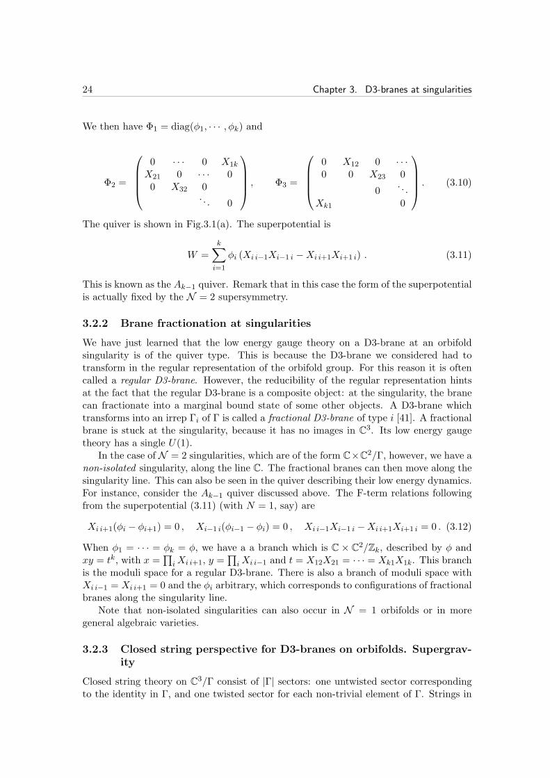
24 Chapter 3. D3-branes at singularities
We then have Φ1 = diag(φ1, · · · , φk) and
Φ2 =
0 · · · 0 X1k
X21 0 · · · 00 X32 0
. . . 0
, Φ3 =
0 X12 0 · · ·0 0 X23 0
0. . .
Xk1 0
. (3.10)
The quiver is shown in Fig.3.1(a). The superpotential is
W =
k∑
i=1
φi (Xi i−1Xi−1 i −Xi i+1Xi+1 i) . (3.11)
This is known as the Ak−1 quiver. Remark that in this case the form of the superpotentialis actually fixed by the N = 2 supersymmetry.
3.2.2 Brane fractionation at singularities
We have just learned that the low energy gauge theory on a D3-brane at an orbifoldsingularity is of the quiver type. This is because the D3-brane we considered had totransform in the regular representation of the orbifold group. For this reason it is oftencalled a regular D3-brane. However, the reducibility of the regular representation hintsat the fact that the regular D3-brane is a composite object: at the singularity, the branecan fractionate into a marginal bound state of some other objects. A D3-brane whichtransforms into an irrep Γi of Γ is called a fractional D3-brane of type i [41]. A fractionalbrane is stuck at the singularity, because it has no images in C
3. Its low energy gaugetheory has a single U(1).
In the case of N = 2 singularities, which are of the form C×C2/Γ, however, we have anon-isolated singularity, along the line C. The fractional branes can then move along thesingularity line. This can also be seen in the quiver describing their low energy dynamics.For instance, consider the Ak−1 quiver discussed above. The F-term relations followingfrom the superpotential (3.11) (with N = 1, say) are
Xi i+1(φi − φi+1) = 0 , Xi−1 i(φi−1 − φi) = 0 , Xi i−1Xi−1 i −Xi i+1Xi+1 i = 0 . (3.12)
When φ1 = · · · = φk = φ, we have a a branch which is C × C2/Zk, described by φ and
xy = tk, with x =∏
iXi i+1, y =∏
iXi i−1 and t = X12X21 = · · · = Xk1X1k. This branchis the moduli space for a regular D3-brane. There is also a branch of moduli space withXi i−1 = Xi i+1 = 0 and the φi arbitrary, which corresponds to configurations of fractionalbranes along the singularity line.
Note that non-isolated singularities can also occur in N = 1 orbifolds or in moregeneral algebraic varieties.
3.2.3 Closed string perspective for D3-branes on orbifolds. Supergrav-ity
Closed string theory on C3/Γ consist of |Γ| sectors: one untwisted sector corresponding
to the identity in Γ, and one twisted sector for each non-trivial element of Γ. Strings in

3.2. D-branes at singularities and quivers 25
the twisted sector are stuck at the orbifold singularity. It is interesting that perturbativestring theory (or more precisely a description of the closed string in term of a N = (2, 2)free CFT) imposes that the period
∫
C B2 on any exceptional curve1 C is fixed [42]. In thepresence of D-branes, we have that [43]
1
4π2α′
∫
Ci
B2 =dim (Γi)
|Γ| ,1
4π2α′
∫
C0
B2 = −∑
i 6=0
dim (Γi)
|Γ| (3.13)
where the exceptional 2-cycles Ci for i 6= 0 are in correspondence with the non-trivialirreducible representations of Γ appearing in (3.5). We have that C0 = −∑i 6=0 Ci inhomology.
We are really interested in only the massless modes of type IIB string theory, so it iseasier to consider just supergravity, taking good notice of the orbifold identification andof the additional twisted fields living on the singular submanifolds. In the supergravitylimit it is certainly natural for
∫
CiB2 to take any value.
Moreover, we have the natural identification of fractional branes with wrapped branes[41]. A fractional D-brane is nothing but a wrapped D-brane on a vanishing cycle. Sucha brane can still have non-zero tension because of a non-zero value for the B-field, as wenow recall, following the review [44]. This is easily seen in the DBI approximation 2. Letus define the quantities
bi = bi + fi ≡1
4π2α′
∫
Ci
(B2 + 2πα′F2
), (3.14)
with F2 the world-volume flux. The Einstein frame action for a probe D(p + 2)-branewrapped on the vanishing 2-cycle Ci is
Si = −τp∫
dp+1ξeΦ−34
√
− det g|bi| + τp
∫
p+1
(
Cp+1bi +Ap+1
)
. (3.15)
The twisted field Ap+1 is defined such that
τp+2
∫
p+3Cp+3 = τp
∫
p+1Ap+1 . (3.16)
Importantly, the wrapped D(p+2)-brane couples to the RR potential Cp+1 with a charge
Q(i)p = bi τp bi ∈ [0, 1) . (3.17)
It is BPS as long as bi is positive, because τ(i)p = |Q(i)
p |. When bi = 0 the fractionalbrane tension vanishes, which can lead to interesting phenomena, some of which are tobe discussed in this thesis. One chooses the background value of B2 + 2πα′F2 on eachcycle Ci, including C0, such that
∑
i bi = 1. This corresponds to the fact that since aregular Dp-brane is a marginal bound state of all the possible fractional branes we shouldhave SDp =
∑
i Si.
1An exceptional curve, or generally an exceptional cycle, is a cycle which would appear in some partialresolution preserving the CY condition (see e.g. section B.4.1 in the Appendix). In the orbifold limit theKahler class of this cycle goes to zero. However, in string theory we have a complexified Kahler classJ + iB which doesn’t need to vanish.
2The DBI action for a D-brane is technically valid only at large volume. However, for N = 2 SUSYpreserving orbifolds we can extrapolate the results from large volume to the orbifold fixed point. WithN = 1 SUSY only the information corresponding to the holomorphic data of the field theory on theD3-branes can be reliably extrapolated to small volume.

26 Chapter 3. D3-branes at singularities
3.3 Branes at generic Calabi-Yau singularities
Having understood the case of an orbifold singularity, we now consider the general prob-lem of finding the low energy field theory for D3-branes at any CY singularity. We canalready anticipate that many of the ingredients of the orbifold case will carry over to thegeneral case: the low energy field theory will be a quiver, and each node of the quiver willcorrespond to some brane wrapped on a vanishing cycle. Such wrapped branes are stillcalled fractional branes. The question is how to find this quiver from the geometric data.In this section (which can be skipped) we consider the general case in a very sketchymanner; in the next sections we consider the case of toric singularities, where a solutioncan be given much more explicitly. The reason we have to be very sketchy in this sectionis that the way to phrase the problem rigorously uses quite a bit of a extra mathematicalmachinery (sheaves and homological algrebra) which is orthogonal to the tools used inthis work. Nevertheless, for the sake of completeness, we will try to convey a rough ideaof the deep relationship between CY singularities and quivers.
Our whole setup preserves N = 1 supersymmetry in four dimensions. The questionwe are really asking is the following: Given a Calabi-Yau threefold singularity, what isthe holomorphic data of the field theory living on a stack of D3-branes located at thesingularity.
• What are the gauge groups and what is the matter content?
• What is the superpotential?
This is what we mean by finding the quiver. Only these pieces of information are encodedin the quiver-with-superpotential structure discussed in this chapter. In particular weare not asking any information about the Kahler potential of the field theory. Theholomorphic structure of the field theory is fully encoded in the holomorphic data of theCY threefold. It is independent of the Kahler structure of the CY3, and it can thus becomputed at large volume in the resolved singularity. This approach was first advocatedby Wijnholt in [45]. See also [46, 47]. The appropriate language to describe D-braneswrapped on holomorphic cycles, at large volume, is the language of B-branes, which arebranes in the topological B-model at gs = 0; see [48, 49] for reviews. Mathematically,B-branes are coherent sheaves. A coherent sheaf is a mathematical object which makeswell defined the notion of a “vector bundle over a holomorphic cycle”. At this levelof discussion, coherent sheaves are just the branes wrapped around points, 2-cycles or4-cycles (D3-, D5-, D7-branes, respectively).
The idea of the large volume perspective is that all the B-branes will correspondto some fractional branes at the singularity in the small volume limit3. One must findsome kind of finite “basis” for the B-branes. Each coherent sheave Ei in that basisshould correspond to a fractional brane, and to a node in the quiver. Moreover, theB-branes “intersect” in a way which can be determined by algebraic geometry. At thesesintersection points we have massless open strings. These open string modes are countedby some generalization of cohomology groups called Ext groups. Between the coherent
3Actually it is not always true, one should usually also perform a so-called stability analysis, whichgoes beyond the B-model computation, to make sure that the B-brane is a good BPS D-brane in thesmall volume limit.

3.3. Branes at generic Calabi-Yau singularities 27
sheaves E and F , we have the groups
Extk(E,F ) , (3.18)
with k = 0, · · · , n for a n-fold. Moreover, for Calabi-Yau n-folds we have the relations
Extk(E,F ) ∼= Extn−k(F,E) , (3.19)
which is called Serre duality; so we only need to compute half of the Ext groups. Thistopological information allows one to read the quiver, in principle. In particular onecan sometimes argue (for instance as in [50]) that the Ext0 groups correspond to aN = 1 vector multiplets in the quiver, while the Ext1 groups correspond to chiral mul-tiplets. So dimExt0(E,E) counts the rank of the gauge group at node E (we shouldhave dimExt0(Ei, Ej) = 0 for i 6= j), and dimExt1(Ei, Ej) counts the number of bifun-damental fields between Ei and Ej . More complicated tricks also allow to compute thesuperpotential in some cases.
In practice any computation is horrendously complicated, and the above programhas been carried out only in the case of complex cones over del Pezzo surfaces dPn,n = 1, · · · , 8 (which are non-toric for n > 3); see also [51]. In that case there is a usefulbasis of B-branes called an exceptional collection which simplifies the problem [45, 47],and one can take advantage of existing mathematical results.
Note also that B-branes have the structure of a category : we have “objects”, theB-branes, and “morphism” between them, the Ext groups. It is in this category languagethat the comparison of B-branes on some geometry with the structure of a quiver becomesvery natural, as we now explain. We are following [52, 53].
3.3.1 Homological algebra and the relation between quivers and singu-larities
Let us consider an abstract quiver with superpotential relations. By abstract quiver wemean that we only consider a graph made of nodes i = 1, · · · , G, and of arrows Xα
between the nodes. A path from i to j is a string of subsequent arrows going from i to j.A quiver relation is a relation between several paths between the same two nodes. We callsuperpotential relation a relation which follows from a superpotential W (Xα), consistingof a formal sum of closed loops with signs 4, so that any relation F can be derived as
FX = ∂XW = 0, (3.20)
for some arrow X. A quiver algebra is just the algebra of paths, CQ, made of all the pathsin the quiver (multiplication is the concatenation of paths), modulo the superpotentialrelations. We designate the relations by the ideal I, so the quiver algebra is
A(Q) = CQ/I . (3.21)
Note that for any quiver with closed loops the path algebra CQ is infinite dimensional,although there are a finite number of generators, which are the arrows themselves.
4W needs to consist of closed loops generically, so that ∂XW relates several paths between the twosame nodes. It is the requirement of gauge invariance in the field theory.

28 Chapter 3. D3-branes at singularities
Of course we could add more structure to this quiver. We could assign a vector spaceEi = C
ni to each node, and assign a linear map (ni × nj matrix)
Xij : Cni → C
nj , i.e. Xij ∈ Hom(Ei, Ej) . (3.22)
to each arrow. We could also assign a gauge symmetry Gl(ni,C) to each node i, actingin the obvious way. But this is some extra information, which is taken care of by theconcept of quiver representation. A quiver representation is a representation of the quiveralgebra, which can be generated by the assignments just made of vector spaces and linearmaps. The set of all representations has the structure of a category: an object is a quiverrepresentation, and a morphism is a set of linear maps between the vector spaces in thetwo quiver representations such that every square commutes 5. This category is so-calledAbelian, and we can go to the derived category. This is not as awful as it sounds, butwe do not have space for definitions here. Suffice to say that the objects in the derivedcategory, which we still denote Ei, are chain complex of the original objects. For instancewe can have the trivial complex
· · · → 0→ Ei → 0→ · · · (3.23)
The relevant morphisms are also called Extn(E,F ), for n = 0, · · · 3 (they are “derivedfunctors of the Hom functor”).
Physically speaking, the objects in this derived category represent the supersymmetricvacua of the quiver, for all possible ranks of the gauge groups. The group Ext0(E,F ) =Hom(E,F ) represent the gauge symmetries which would remain unbroken if you tried tocombine objects E and F , while Ext1(E,F ) is best thought as the physical modes (gaugeequivalence class of modes satisfying the quiver relations) you can turn on between Eand F . Lastly the elements of Ext2(E,F ) are related to the quiver relations themselves.Now, for a quiver with superpotential relations it is possible to prove that [53]
Ext1(E,F ) ∼= Ext2(E,F ) , (3.24)
which follows from the fact that X and FX are somewhat “dual” because every relationfollow from a superpotential 6.
If we want to identify this quiver category structure with the B-brane category struc-ture on a Calabi-Yau n-fold, we need that n = 3 because of (3.24) and (3.19). The preciseconjecture is that the derived category of quiver representations is isomorphic to the B-brane category (which is actually also a derived category) on a Calaby-Yau threefold, atleast in the case of a quiver with generic superpotential.
3.4 Hanany-Witten setups
In this section we succinctly discuss some systems of D4-branes suspended between NS5-branes, which are T-dual to systems of D3-branes on generalised conifolds in type IIB.In general, such Hanany-Witten setups [54] provide a very useful point of view on some
5The category of quiver representations is isomorphic to the category of A(Q)-modules.6Actually this Serre relation holds only for certain superpotentials, such that every fractional brane
representation has a projective resolution; for instance if W = 0 this is not the case [53].
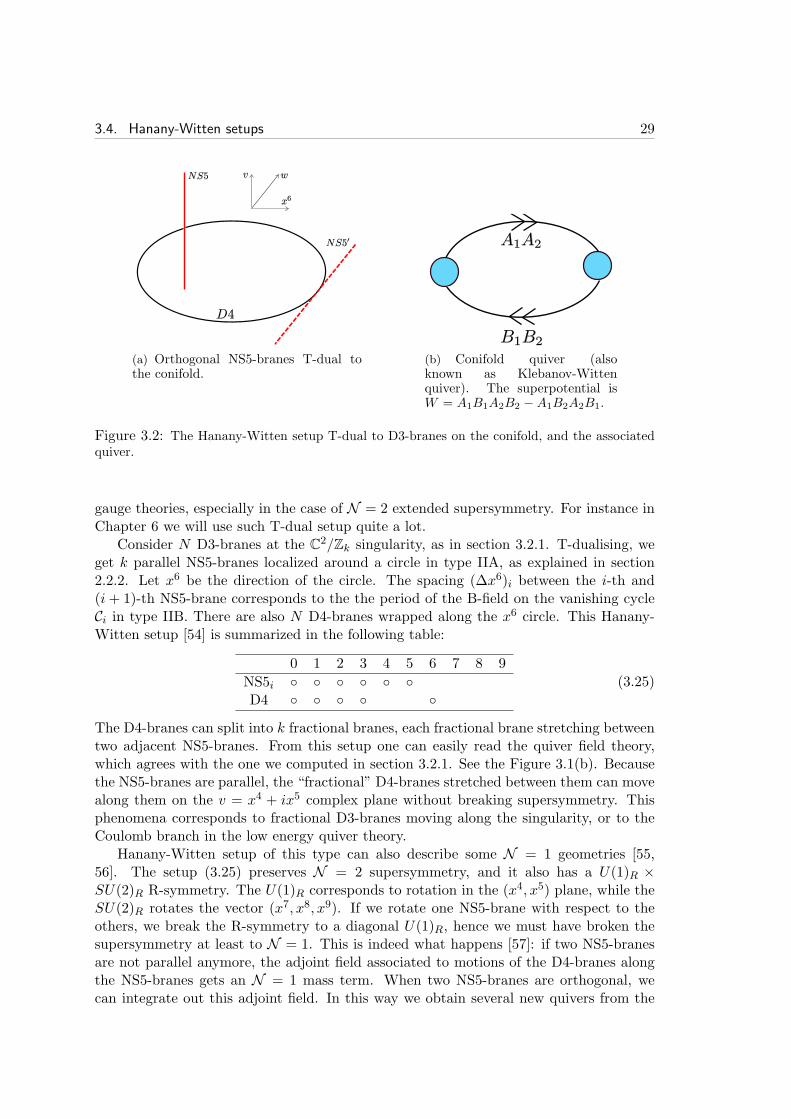
3.4. Hanany-Witten setups 29
(a) Orthogonal NS5-branes T-dual tothe conifold.
(b) Conifold quiver (alsoknown as Klebanov-Wittenquiver). The superpotential isW = A1B1A2B2 −A1B2A2B1.
Figure 3.2: The Hanany-Witten setup T-dual to D3-branes on the conifold, and the associatedquiver.
gauge theories, especially in the case of N = 2 extended supersymmetry. For instance inChapter 6 we will use such T-dual setup quite a lot.
Consider N D3-branes at the C2/Zk singularity, as in section 3.2.1. T-dualising, we
get k parallel NS5-branes localized around a circle in type IIA, as explained in section2.2.2. Let x6 be the direction of the circle. The spacing (∆x6)i between the i-th and(i+ 1)-th NS5-brane corresponds to the the period of the B-field on the vanishing cycleCi in type IIB. There are also N D4-branes wrapped along the x6 circle. This Hanany-Witten setup [54] is summarized in the following table:
0 1 2 3 4 5 6 7 8 9
NS5i D4
(3.25)
The D4-branes can split into k fractional branes, each fractional brane stretching betweentwo adjacent NS5-branes. From this setup one can easily read the quiver field theory,which agrees with the one we computed in section 3.2.1. See the Figure 3.1(b). Becausethe NS5-branes are parallel, the “fractional” D4-branes stretched between them can movealong them on the v = x4 + ix5 complex plane without breaking supersymmetry. Thisphenomena corresponds to fractional D3-branes moving along the singularity, or to theCoulomb branch in the low energy quiver theory.
Hanany-Witten setup of this type can also describe some N = 1 geometries [55,56]. The setup (3.25) preserves N = 2 supersymmetry, and it also has a U(1)R ×SU(2)R R-symmetry. The U(1)R corresponds to rotation in the (x4, x5) plane, while theSU(2)R rotates the vector (x7, x8, x9). If we rotate one NS5-brane with respect to theothers, we break the R-symmetry to a diagonal U(1)R, hence we must have broken thesupersymmetry at least to N = 1. This is indeed what happens [57]: if two NS5-branesare not parallel anymore, the adjoint field associated to motions of the D4-branes alongthe NS5-branes gets an N = 1 mass term. When two NS5-branes are orthogonal, wecan integrate out this adjoint field. In this way we obtain several new quivers from the
30 Chapter 3. D3-branes at singularities
one of Figure 3.1(a) for C × C2/Zk: we simply integrate out any pair of adjoint fields
for the two gauge groups located on each side of the NS5-brane which we rotate. Let ussay we rotate several NS5-branes onto the w = v8 + ix9 direction, and we call these theNS5’-branes. We have
0 1 2 3 4 5 6 7 8 9
NS5i NS5’j D4
(3.26)
The simple example of the conifold geometry xy − vw = 0 is depicted in Figure 3.2, to-gether with the associated quiver with superpotential. The superpotential can be deducedfrom the superpotential of the N = 2 quiver by giving a mass to the adjoint fields andintegrating them out. In general, this setup can describe D3-branes on any generalisedconifold of the form
xy − vmwn = 0 . (3.27)
For m = 0 we have the N = 2 case, C2/Zn. In general, we can see this geometry asa cylinder C
∗ fibered over C2 ∼= v, w according to the equation xy = f(v, w). When
f(v, w) = 0 the S1 of the cylinder pinches off. If we T-dualise along this S1 the loci wherethe fiber degenerates corresponds to the locations of the T-dual NS5-branes [58]. For thegeneralized conifold, f(v, w) = vmwn so that there are n NS5-branes along v (at wn = 0)and m NS5-branes along w (at vm = 0) in the T-dual.
Remark that from this T-duality argument we cannot specify the ordering of thevarious NS5 and NS5′ branes along the x6 circle. This is because such ordering dependson information about the Kahler structure (in particular about periods of the B-field).
3.5 Toric singularities and dimer models
Toric Calabi-Yau singularities form a very simple class of Calabi-Yau singularities (seeAppendix B for an introduction). It is only natural to try to find the quiver for any toricCY singularity by taking advantage of the tools of toric geometry. This problem was firstadressed in [59]; in this early approach, one embeds any toric singularity X into a largerC3/(Zn × Zm) singularity. The quiver of the parent orbifold is known, and one finds the
quiver of X by Higgsing the orbifold quiver (corresponding to partial resolution in thegeometry).
A few years ago a breakthrough was made thanks to the work of Hanany, Kennawayand collaborators [60, 61]. These papers found a beautiful underlying combinatoric struc-ture to the so called toric quivers, which makes the translation between toric geometryand quivers very deep and surprisingly simple. The structure which made this simplifi-cation possible is known as brane tiling (and the associated dimer model). A lot of workfollowed, some of which will be reviewed in this section.
We are mainly concerned with the determination of the geometry associated to anytoric quiver. For more comprehensive introduction to the subject, we refer to the beautifulreview [62] by Kennaway.

3.5. Toric singularities and dimer models 31
(a) Periodic quiver. The signs cor-respond to the signs of the terms inthe superpotential.
(b) Brane tiling of the torus. The fun-damental domain is indicated in red.
Figure 3.3: The periodic quiver and the brane tiling for the conifold quiver theory.
3.5.1 Toric quiver theories as dimer models
Toric quivers are a particular type of quiver which satisfy one additional condition: eachchiral field of the quiver appears only linearly in the superpotential, in exactly two termswith opposite signs. This implies that all the F-term relations take the form “monomial= monomial”. For such a quiver, one can define a so-called planar quiver as follows[62]. Consider each superpotential term as a polygon. Give each polygon a positiveor negative orientation according to the sign of the superpotential term, and glue thepolygons together along common arrows. Since each field appears only twice, we thenform an orientable Riemann surface, with the orientation inherited from the orientationof the polygons. We will assume that this Riemann surface is actually a torus (we canactually prove that by assuming conformality of the theory on the D3-branes, as will bediscussed in the next chapter). This graph on the torus is the planar graph. We couldalso have drawn a bi-periodic tiling of the plane by repeating polygons; that graph iscalled the “periodic quiver”.
It is more interesting to consider the graph dual to the planar graph: each polygonwith positive (resp. negative) orientation becomes a white (resp. black) vertex, and eachquiver node becomes a face. This dual graph is bipartite graph on the torus called abrane tiling in the literature. An example is given in Figure 3.3. The dictionary betweenquiver and brane tiling is summarized in Insert 1. Given a brane tiling, a dimer is justa distinguished edge. A perfect matching is a configuration of dimers such that everyvertex is touched exactly once. We define the perfect matching matrix Mαk as
Mαk =
1 if the perfect matching pk contains the fields Xα
0 otherwise(3.28)
A dimer model is nothing but a brane tiling together with its perfect matchings.
32 Chapter 3. D3-branes at singularities
Insert 1. Quiver from brane tiling
A brane tiling is a bipartite graph on the torus: it has white and black vertices inequal numbers, and non-intersecting edges connecting white to black vertices.
• Each face i corresponds to a gauge group.
• Each edge corresponds to a chiral field Xij . Looking towards the white dot, theedge Xij is a field in the fundamental of the gauge group i on its right and inthe anti-fundamental of the gauge group j on its left.
• Each white (black) vertex corresponds to a single-trace superpotential term withthe fields appearing in clockwise (counterclockwise) order, and with a plus (mi-nus) sign in front.
3.5.2 From quiver to geometry: moduli space and the forward algo-rithm
There are many interesting applications of brane tilings and of the associated dimermodels. Here we are mainly concerned with its use to solve for the classical moduli spaceof the Abelian theory [63]. This so-called forward algorithm [60, 61] built on the previouswork [64, 65, 59].
There is a simple rule of thumb to see if a quiver can describe D3-branes at a CY3
singularity: the vacuum moduli space should contain at least the CY threefold. Thisis because regular D3-branes are point-like probes of the geometry, and they can bedisplaced away from the singularity without breaking supersymmetry. Recall that themoduli space of a N = 1 supersymmetric theory is a complex manifold of the form
M = Xα | dW = 0 ; D = 0/G . (3.29)
We first impose the F-flatness conditions dW = 0 on C[Xα], where Xα are the complexscalars in the chiral multiplets. The resulting complex manifold Z was called the “masterspace” in recent literature [66]. Next we impose gauge invariance under the gauge groupG together with the D-flatness conditions D = 0; equivalently one can just quotient bythe complexified gauge group GC [67] (in other words there is an equivalence between theKahler quotient Z//G and the holomorphic quotient Z/GC).
The forward algorithm allows to compute efficiently the Abelian moduli space of anytoric quiver. In the Abelian theory the gauge group is U(1)G. Hence, if W = 0 (forinstance in the Abelian conifold theory) the moduli space (3.29) has an obviously toricdescription as a GLSM (see Appendix B). For a non-trivial superpotential satisfying thetoric condition, the master space itself should be a toric variety, because it has an affinedescription with relations of the form “monomial = monomial”. The master space canthen be described as a GLSM as well. The non-trivial problem is to find the correct set ofhomogeneous coordinates for any quiver. As we will show, the perfect matchings actuallydo the job, although they usually give a redundant set of homogeneous coordinates.

3.5. Toric singularities and dimer models 33
Given a brane tiling, let us assign a complex field pk (so called complex matchingvariable) to each perfect matching. Then assign to each quiver field a product of perfectmatching variables, according to
Xα =∏
k
pMαkk . (3.30)
Due to the toricity condition on the superpotential, any F-term relation ∂XαW = 0 is ofthe form ∏′
β∈VmXβ =
∏′
γ∈VnXγ (3.31)
where∏′ means that the product does not include the fieldXα linking the vertices Vm and
Vn. Using the parametrization (3.30) solves the F-term relations because∏′β∈Vm
Xβ =∏
k p∑′β∈Vm
Mβk
k , and∑′
β∈VmMβk =
∑′γ∈Vn
Mγk = 1 (or 0) ∀k, by the definition of perfectmatching.
Then, we can easily construct a GLSM in term of the perfect matching variables.First there are the charges QD associated to the U(1)G gauge group of the quiver. Let Ebe the number of quiver fields (edges in the brane tiling) and m be the number of perfectmatching variables. Then QD is a (G − 1) × m matrix (QD)
ik which gives the charges
of the pk’s under the quiver gauge group (we really have only a U(1)G−1 gauge groupbecause the diagonal U(1) does not couple to any field). It is defined as
Mαk(Q
tD)
ki = (Qt) αi (3.32)
in term of the perfect matching matrix and of the charge matrix Qiα of the quiver. Thedefinition of QD is only up to elements of kerM . This ambiguity is fixed by intoducingadditional charges
QtF = kerM ; i.e. Mαk(Q
tF )
kl = 0 , (3.33)
which are charges for the perfect matching variables which give zero charge to the quiverfields, according to the map (3.30). They are thus gauge symmetries (redundancies) ofthe parametrization (3.30). The GLSM is thus
p1 · · · pm FI
U(1)lF (QF )l1 · · · (QF )
lm 0
U(1)iD (QD)i1 · · · (QD)
im ξi
(3.34)
Note that we have also considered FI parameters here; however we do not have FI pa-rameters for the U(1)F symmetries because they are not associated to dynamical gaugefields. It turns out that there are m − G − 2 charges QF
7. In total, the GLSM hasm− 3 U(1)’s, so that the resulting space is a 3 dimensional toric variety. Actually it is aCalabi-Yau, since
∑mk=1(QD)
ik = 0, and
∑mk=1(QF )
lk = 0 too. The latter relation follows
from the definition (3.33) and the fact that if we choose all the fields Xγ which end onthe same vertex we have that
∑
γMγk = (1, · · · , 1) (all the perfect matchings are chosenonce), which implies the result.
7It is an “experimental” observation [59, 66] that the master space of toric quivers has dimensionG + 2. I am not aware of any proof in the literature (although see [63]). I thank Amihay Hanany forcorrespondence on this point.
34 Chapter 3. D3-branes at singularities
Recall that, once given the GLSM charges Qt = (QtF , QtD), we can find the vectors of
the toric cone v = (vx, vy, 1),
G =
v(1)x v
(2)x · · · v
(m)1
v(1)y v
(2)y · · · v
(m)y
1 1 · · · 1
, (3.35)
simply by taking the kernel of Q,QGt = 0 . (3.36)
The third line of (3.35) can be chosen so due to the CY condition. Note that we havechosen m toric vectors corresponding to the m homogeneous coordinates (pk), but ingeneral this is not a minimal presentation of the toric diagram (several toric vectors willbe identical). For the physical meaning of these redundancies, see e.g. [62].
3.5.3 Kasteleyn matrix and fast forward algorithm
The remaining question is how to find the perfect matching variables for a given branetiling. The answer is provided by the Kasteleyn matrix [68, 60], which we now review.Let us draw the bipartite graph on a fundamental domain, and denote γx and γy the twoboundaries with orientation, which are particular representatives of the two primitivehomology 1-cycles of the torus. Let us also denote by m,n = 1, · · · , V the white andblack vertices. Let Xa
mn be the edges linking the white node m to the black node n.Finally, let < X, γ > be the intersection number of the edge X with the 1-cycle γ. Theimproved Kasteleyn matrix is defined as
Kmn =∑
γ
Xγmn x
<Xamn,γx>y<X
amn,γy> . (3.37)
The perfect matching are enumerated by the permanent8 of Kmn, which is defined simi-larly to the determinant but with no minus signs,
permK =∑
i1,...,in
(ǫi1...in)2Ki11 . . .Kinn . (3.38)
This permanent is known as the characteristic polynomial of the dimer model. It can bewritten as
permK(x, y) =∑
kpk x
<pk,γx>y<pk,γy> , (3.39)
where each summand pk is a perfect matching, written as
pk =∏
αXMαkα . (3.40)
Note that one should not take this notation seriously, unlike in the relation (3.30); perfectmatching are only a collection of edges, and would be more properly written as
pk = Xα |Mkα = 1 . (3.41)
8We could also work with the determinant, but at the cost of introducing some extra signs in thedefinitions.
3.5. Toric singularities and dimer models 35
Insert 2. The fast forward algorithm
The fast forward algorithm [60, 61] is a very efficient way to find the toric diagramcorresponding to the Abelian moduli space of a toric quiver. Given a brane tiling, wedefine the Kasteleyn matrix. Each row of this matrix represents a white node, eachcolumn a black node. Each entry is a sum of monomials
Kmn =∑
γ ∈m→n
Xγ x<Xγ ,γx>y<Xγ ,γy> (3.44)
where we sum over the edges Xγ which go from the white node m to the black noden; x, y are formal parameters and < Xγ , γx >, < Xγ , γy > are the number of times,with sign, the field Xγ crosses the x and y boundaries of the fundamental domain.The perfect matching are found through the permanent (a determinant without theminus signs)
permK =∑
kpk x
hx(k)yhy(k) . (3.45)
The set of points (hx, hz) in Z2 (sometimes called the Newton polygon of the polyno-
mial permK) is the toric diagram of the Calabi-Yau threefold we are looking for!A change of fundamental domain (which changes the values of the < Xγ , γx,y >)corresponds to a Sl(3,Z) transformation of the toric diagram.
The coefficientshx(pk) =< pk, γx > , hy(pk) =< pk, γy > , (3.42)
are called the slopes of the perfect matching pk. They represent the flux that goes out ofthe fundamental domain through γx or γy, for a given perfect matching pk:
hx(pk) =∑
α
Mkα < Xα, γx > , hy(pk) =∑
α
Mkα < Xα, γy > . (3.43)
This construction actually gives us more than just the perfect matchings. It directlygives us the toric diagram. This so-called fast forward algorithm is summarized in theInsert 2. The claim of [61], proven in [63], is that the points (hx, hy) ∈ Z
2 are preciselythe points of the toric diagram for the CY3 associated to the brane tiling. To prove that,we need to prove that the matrix
Gh =
hx(p1) hx(p2) · · · hx(pm)hy(p1) hy(p2) · · · hy(pm)
1 1 · · · 1
(3.46)
is the same (or Sl(2,Z) equivalent) to the matrix G defined in (3.35). In other words, weneed to prove that
QF Gth = 0 , and QDG
th = 0 . (3.47)
The first equality directly follows from (3.43) and (3.33). To prove the second equality,we note that, using (3.43) and (3.32),
(QD)ik(G
th)kx = (QD)
ikM
kα < Xα, γx >=
∑
αQiα < Xα, γx > , (3.48)
36 Chapter 3. D3-branes at singularities
with Qiα is the charge matrix of the quiver. We then easily show that the l.h.s. is zero ∀i[63]. Suppose all the edges in the brane tiling are bifundamental fields (the incorporationof adjoint fields is straightforward). For each face i in the tiling, there are an even numberof edges X which cross γx. Consider two edges X and X ′ in X which are consecutiveas we go around the face i. From the definition of a brane tiling, we have that the chargesQi(X) and Qi(X ′) are the same (resp. of opposite sign) if the X and X ′ are separated byan odd (resp. even) number of edges. On the other hand < X, γx > and < X ′, γx > haveopposite (resp. same) sign if the separation is odd (resp. even). Hence the contributionof X and X ′ cancels out in (3.48). The same reasoning holds for the y component. Thiscompletes the proof.
3.5.4 An example: the dP1 quiver.
Let us work out an example, to see how the above concepts drastically simplify thecomputation of the moduli space. We consider the somewhat famous dP1 quiver [59].It is a quiver corresponding to D3-branes at the tip of a complex cone over the first delPezzo surface9, CC(dP1) (which is also the real cone over Y 2,1). The quiver is shown inFig. 3.4(a). The superpotential is
W = ǫabXa12X
b23X31 + ǫabXa
41Xb12X24 + ǫabX3
12Xa23X34X
b41 (3.49)
From the corresponding brane tiling shown in Fig. 3.4(b), we write down the Kasteleynmatrix,
K =
X223 X31 X1
12 x−1y
X34 +X312 y
−1 X123 X2
41
X141 X2
12 x X24
(3.50)
and its permanent
permK =(X1
12X212X
312 +X1
23X223X24 +X24X31X34 +X31X
141X
241
)+
+X212X
223X
241 x+X3
12X24X31 y−1 +X1
12X212X34 y +X1
12X123X
141 x
−1y . (3.51)
The resulting 2d toric diagram (made of 5 points) is shown in Figure 3.4(c). The perfectmatchings10 and the corresponding points in the toric diagram are
a = X212, X
223, X
241 = (1, 0, 0) , e = X1
12, X212, X
312 = (0, 0, 0) ,
b = X112, X
212, X34 = (0, 1, 0) , f = X1
23, X223, X24 = (0, 0, 0) ,
c = X112, X
123, X
141 = (−1, 1, 0) , g = X24, X31, X34 = (0, 0, 0) ,
d = X312, X24, X31 = (0,−1, 0) , h = X31, X
141, X
241 = (0, 0, 0) .
(3.52)
The F-term relations of the theory are solved by
X112 = bce , X1
41 = ch , X123 = cf , X34 = bg ,
X212 = abe , X2
41 = ah , X223 = af ,
X312 = de , X31 = dgh , X24 = dfg ,
(3.53)
as one can easily check.
9The corresponding AdS/CFT duality was first discussed in [69, 70].10We denote (pk) = (a, b, · · · , h) for later use in Chapter 13.
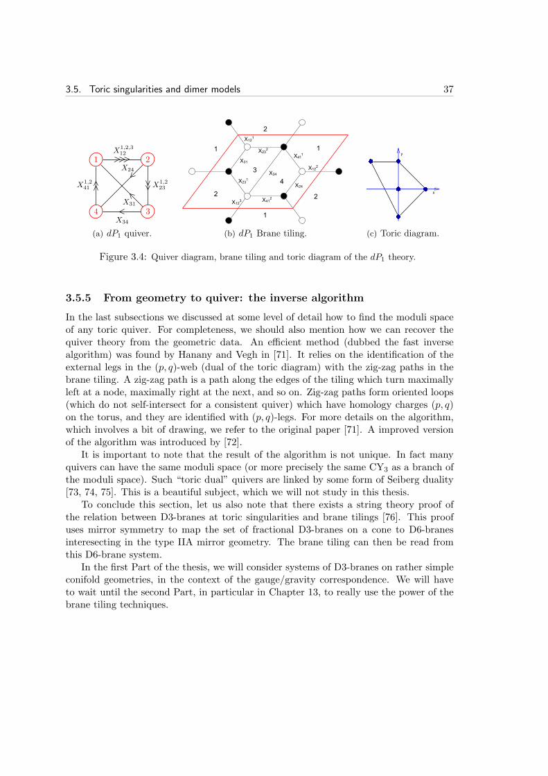
3.5. Toric singularities and dimer models 37
(a) dP1 quiver. (b) dP1 Brane tiling. (c) Toric diagram.
Figure 3.4: Quiver diagram, brane tiling and toric diagram of the dP1 theory.
3.5.5 From geometry to quiver: the inverse algorithm
In the last subsections we discussed at some level of detail how to find the moduli spaceof any toric quiver. For completeness, we should also mention how we can recover thequiver theory from the geometric data. An efficient method (dubbed the fast inversealgorithm) was found by Hanany and Vegh in [71]. It relies on the identification of theexternal legs in the (p, q)-web (dual of the toric diagram) with the zig-zag paths in thebrane tiling. A zig-zag path is a path along the edges of the tiling which turn maximallyleft at a node, maximally right at the next, and so on. Zig-zag paths form oriented loops(which do not self-intersect for a consistent quiver) which have homology charges (p, q)on the torus, and they are identified with (p, q)-legs. For more details on the algorithm,which involves a bit of drawing, we refer to the original paper [71]. A improved versionof the algorithm was introduced by [72].
It is important to note that the result of the algorithm is not unique. In fact manyquivers can have the same moduli space (or more precisely the same CY3 as a branch ofthe moduli space). Such “toric dual” quivers are linked by some form of Seiberg duality[73, 74, 75]. This is a beautiful subject, which we will not study in this thesis.
To conclude this section, let us also note that there exists a string theory proof ofthe relation between D3-branes at toric singularities and brane tilings [76]. This proofuses mirror symmetry to map the set of fractional D3-branes on a cone to D6-branesinteresecting in the type IIA mirror geometry. The brane tiling can then be read fromthis D6-brane system.
In the first Part of the thesis, we will consider systems of D3-branes on rather simpleconifold geometries, in the context of the gauge/gravity correspondence. We will haveto wait until the second Part, in particular in Chapter 13, to really use the power of thebrane tiling techniques.


Part I
Gauge/gravity and cascades
39


Chapter 4
Conformal field theories and theAdS/CFT correspondence
This Chapter gives an introduction to the AdS/CFT correspondence. Particular focusis put on the case of the AdS5/CFT4 correspondence, stemming from properties of D3-branes. The general discussion of subection 4.3.3 also holds for the case of the dualitystemming from M2-branes, which we discuss in the second Part of the thesis.
4.1 Superconformal gauge theories in 3+1 dimensions
It is known since the work of Coleman and Mandula [77] that a non-trivial QFT cannotenjoy arbitrary space-time symmetries. In the presence of massive fields the most generalbosonic symmetry is the Poincare symmetry. If all the fields are massless, we can also haveconformal symmetry. Conformal transformations are transformations which preserve thebackground metric up to an overall factor, gµν(x)→ eω(x)gµν(x).
The conformal group of d dimensional Minkowski space-time consists of the Poincaregroup together with scale transformations and the special conformal transformations,
xµ → λxµ , xµ → xµ + aµx2
1 + 2aνxν + a2x2. (4.1)
Let us denote byMµν and Pµ the Poincare generators (Lorentz transformations and trans-lations), by D the scale transformation and by Kµ the special conformal transformations.The conformal algebra is actually isomorphic the SO(d, 2) algebra,
[Jab, Jcd] = iηacJbd + iηbdJac − iηadJbc − iηbcJad . (4.2)
Here a = (µ, d, d + 1), and we use the metric ηab = diag(− + · · · + −). The so(d, 2)generators are
(Jab) =
Mµν12(Kµ − Pµ) 1
2(Kµ + Pµ)−1
2(Kν − Pν) 0 −D−1
2(Kν + Pν) D 0
(4.3)
41

42 Chapter 4. Conformal field theories and the AdS/CFT correspondence
4.1.1 N = 1 superconformal algebra
Combining conformal transformations with N -extended supersymmetry in four dimen-sions, one obtains the superconformal group SU(2, 2|N ). In the following we focus onthe N = 1 case. The generators of the N = 1 superconformal algebra can be organisedaccording to their scaling dimensions. We have
PµQα Qα
∆ Mµν RSα Sα
Kµ
The elements of the super-Poicare subalgebra are the top ones: Pµ, Q, Q and Mµν havescaling dimension 1, 1
2 ,12 and 0, respectively. Special conformal transformations Kµ have
dimension −1. We also have dilatation and R-symmetry generators ∆ and R, both ofdimension 0, and finally the conformal supersymmetry generators S and S.
One can consider several real forms of this algebra. For doing quantum field theorywe need a self-adjoint Hamiltonian. In Minkowsky space-time we then require that Q† =Q, so that P †
µ = Pµ, and similarly for S, S and Kµ. However this is not the mostconvenient way to deal with a CFT, because we cannot really define useful asymptoticstates. Instead, we go with to the Euclidian theory on R
4 and we consider correlationfunctions of operators, much like for a statistical mechanical system. Consider then R
4
minus the origin. We can do a conformal transformation to the cylinder R× S3,
dr2 + r2dΩ23∼= dτ2 + dΩ2
3 , (4.4)
with r = eτ , and then go to real time again, τ = it. Then ∆ = r∂r = −i∂t = H ′, namelythe dilatation operator on R
4 becomes an Hamiltonian on the cylinder. For this H ′ to beself-adjoint we must consider a real form of the algebra where P †
µ = Kµ and Q†α = Sα.
This is called the radial quantization picture.Any local operator in the Euclidean picture corresponds to a state on the cylinder.
Indeed any operator insertion at the origin of R4 corresponds to a boundary condition att = −∞,
|O〉 = limr→0O|0〉 . (4.5)
Conversely, we can take any state on S3, consider it as a field configuration on some ballaround the origin, and shrink the ball to zero size thanks to conformal invariance. Thisis the state-operator correspondence of conformal field theory.
In the radial quantization picture, one can derive interesting bounds from unitarity.In particular ∆ ≥ 1 for scalar operators in any CFT. In any N = 1 SCFT we also havethe important bound [78]
∆ ≥ 3
2|R| (4.6)
for any scalar operator. The R-charge is normalized so that [R,Q] = −Q.We now introduce the notion of primary and superprimary operators. Operators in
the theory will appear in representations of the (super)conformal algebra. Notice thenthat Kµ lowers the conformal dimension of a field by −1. Hence, because there is a lower
4.1. Superconformal gauge theories in 3+1 dimensions 43
bound on ∆ in a CFT, a conformal multiplet must have a lowest component, such that[Kµ,Op] = 0. Such a Op is called a primary operator. Similarly, in a SCFT, Sα andSα lower the dimensions by −1
2 . A superprimary operator is the lowest component of asuperconformal multiplet, i.e. it is such that
[S,Osp]± = 0 . (4.7)
Any superprimary is also a primary. An operator which can be written as [Q,O] is calleda superconformal descendant. So a superconformal multiplet consist of one superprimaryoperator and several descendants.
We are also interested in short representations of the superalgebra, which are calledBPS or chiral multiplets, which are annihilated by some of the Q’s. The lowest componentof a chiral multiplet is called a chiral superprimary, or chiral primary for short. It saturatesthe bound (4.6) as ∆ = 3
2R. The dimension of a chiral primary is then protected fromquantum corrections.
4.1.2 N = 4 SYM
The N = 4 Super-Yang-Mills theory is the maximally (rigid) supersymmetric theory infour dimension. Its Lagrangian can easily be worked out from dimensional reduction ofmaximally supersymmetric 10 dimensional SYM, for instance. In N = 1 notation, itreads (traces are implicit)
L =
∫
d2θd2θ3∑
i=1
ΦieV Φ†
i +
∫
d2θ( τ
16πiW2 + gΦ1[Φ2,Φ3]
)
+ h.c. (4.8)
All the fields are in the adjoint representation of SU(N). It has a high degree of symmetry,the superconformal group PSU(2, 2|4), whose maximal bosonic subgroup is SO(4, 2) ×SU(4). The six real scalar fields φi (Φ1 = φ1 + iφ2, etc.) are in the 6 of the R-symmetrygroup SU(4) ∼= SO(6). According to the NSVZ beta function (cfr Appendix C), thegauge coupling is exactly marginal in perturbation theory, β(g) = 0. Indeed b0 = 0, andthe anomalous dimension for the chiral superfields must vanish by symmetry.
There is also strong evidence that this theory enjoys Montonen-Olive duality [79], alsoknown as S-duality, exchanging strong and weak coupling, as τ → − 1
τ . Combining withthe equivalence τ → τ + 1 which shifts the θ angle by 2π, the conjecture is that N = 4SYM is invariant under any Sl(2,Z) transformation of its gauge coupling,
τ → aτ + b
cτ + d,
(a bc d
)
∈ Sl(2,Z) . (4.9)
From the perspective of string theory, this is quite natural. N = 4 SYM is the theoryliving on a bunch of flat D3-branes, and we have the identification τ = C0+ i/gs betweenthe gauge coupling and the background value of the axio-dilaton. Montonen-Olive dualityis then inherited from the S-duality of type IIB string theory (under which the D3-braneis self-dual).
As an important remark, note that although the gauge group on N D3-branes isU(N), the diagonal U(1) is free and can be decoupled in the IR. We will come back tothis point later on.

44 Chapter 4. Conformal field theories and the AdS/CFT correspondence
4.1.3 An example of an N = 2 SCFT
Generically theories with less supersymmetries are not conformal. However for particularfield contents we can still tune all the beta functions to vanish, and hope (and hopefullycheck!) that the theory is really a superconformal field theory. An example which willbe of particular interest to us in Chapter 6 is N = 2 SU(N) SQCD with Nf = 2Nfundamental hypermultiplets. In N = 1 language, it contains one chiral superfield Φin the adjoint representation, 2N chiral superfields Q in the fundamental and 2N chiralsuperfields Q in the anti-fundamental. Again, one can check that b0 = 0 so the betafunction vanishes at one loop. Actually, using the Seiberg-Witten theory one can arguethat the theory is exactly superconformal [80]. It is also thought to enjoy Montonen-Oliveduality.
This example of Nf = 2N N = 2 SQCD is actually an example of a continuous familyof conformal field theories, indexed by the coupling τ which is exactly marginal. It iscalled a line of fixed points in coupling space. The SCFT we will consider in the first partof this work will also have this property of being part of a continuous line of fixed point.This is because we will consider theories which have an AdS5 dual under the AdS/CFTmap, and in all the cases the dual AdS5 solution comes in a continuous family indexedby the VEV of the axio-dilaton.
In general, however, conformal field theories only exist as isolated fixed points incoupling space. The typical N = 2 example is the Argyres-Douglas fixed point [81] (seealso [82]). Anticipating, we note that this fact will be important in the second part ofthis work, which deals with SCFTs in three space-time dimensions. These theories willtypically be isolated fixed points, and this is dual to the statement that the AdS4 solutionsof M-theory usually do not have marginal directions.
4.1.4 N = 1 SCFT: an example of a strongly coupled fixed point
In four dimensional theories with extended supersymmetry, the line of fixed points alwaysgoes through the origin in coupling space, so that these theories can be made arbitrarilyweakly coupled. In N = 1 theories we can have more general families of CFTs whichhave no weak coupling limit. Consider for instance an N = 1 SU(N) theory with Nf =2N flavors, namely Nf fundamental fields Qi and Nf antifundamental fields Qj , with asuperpotential of the form [83, 84]
W = h(QiQj)(QjQ
i) . (4.10)
Due to the flavor symmetry all the fields Qi and Qi must have the same anomalousdimension γ0. The beta functions are proportional to each others,
β(h) = (1 + 2γ0)h , β
(8π2
g2
)
= N(1 + 2γ0) . (4.11)
Hence the conditions for vanishing beta functions reduce to the single equation γ0(h, g) =−1
2 in a two dimensional coupling space. Although we cannot compute γ0(h, g) in general,we can show that this line does not go through the origin by using Seiberg’s conjectureabout a the existence of a non-trivial CFT in N = 1 SQCD, namely at h = 0 [83]: sinceγ0(0, g) = −1
2 has a solution for g = g∗ > 0, the line of fixed point γ0(h, g) = −12 never
goes through the origin. Consequently, the theory is always strongly coupled.

4.2. Anti-de-Sitter space and near horizon limit 45
Note that the superpotential (4.10) is not renormalizable. Consequently the theoryneeds some UV completion to be well defined. Actually there is the interesting optionof embedding it into the finite N = 2 Nf = 2N SQCD [84]. This later theory can bedeformed to N = 1 by a mass term for the adjoint superfield Φ,
W = gQΦQ+1
2mΦ2 . (4.12)
Integrating out Φ, one recovers1 the superpotential (4.10). Recalling that there is a S-duality symmetry in the N = 2 theory, we can ask whether this property is inherited bythe N = 1 theory one obtains by mass deformation. The answers turns out to be positive:Seiberg duality maps the theory (4.10) to itself! These issues are discussed with greatcare in the original paper [84], as well as in [85], to which we refer for further details.
4.2 Anti-de-Sitter space and near horizon limit
Anti-de-Sitter (AdS) space is a maximally symmetric solution to Einstein equations witha negative cosmological constant Λ [86]. The metric for AdS space in d + 1 space-timedimensions reads
ds2(AdSd+1) = R2(− cosh2 ρdτ2 + dρ2 + sinh2 ρdΩ2
d−1
), (4.13)
with the AdS radius R2 = −d(d − 1)/2Λ. These are the so-called global coordinates.The time coordinate τ goes from −∞ to +∞, as part of our definition of the space (weare really considering the universal cover of AdSd+1). The AdS boundary is at ρ → ∞,and it has the form R × Sd−1. The isometry group of AdS is SO(4, 2), the same as theconformal group in d space-time dimensions2. Instead of working in global AdS, we willonly work on the so-called Poicare patch, which covers only half of AdS. The Poincarecoordinates metric is
ds2 =R2
r2dr2 +
r2
R2(ηµνdx
µdxν) . (4.14)
The boundary at r →∞ is just Minkowski space-time Md,1. Note that we took x and rto be dimensionful coordinates (x/R and r/R being dimensionless). For more details onthe AdS space in our context, we refer to [38] and references therein.
4.2.1 Near horizon limit for D3-branes
Consider the p = 3 extremal p-brane solution (2.9), corresponding to N D3-branes in flatspace. The string frame metric is
ds2 = h−12 ηµνdx
µdxν + h12(dr2 + r2dΩ2
5
). (4.15)
1Actually one obtains W = h(
(QQ)(QQ)− 1N(QQ)2
)
because Φ is in the adjoint of SU(N) and not
of U(N), but this subtlety will not concern us.2Note that actually SO(4, 2) is the isometry of the AdS with compact time and not of its universal
cover, so we really mean the algebra so(4, 2). The same comment applies when we consider the symmetrygroup of field theories: we actually never consider global issues, only the algebras.
46 Chapter 4. Conformal field theories and the AdS/CFT correspondence
There is a constant dilaton eΦ = gs, and a 4-form potential C4 = g−1s h−1dx0 ∧ · · · ∧ dx3.
The warp factor h is given by
h(r) = 1 +R4
r4, with R4 =
π3
Vol(S5)4πα′2gsN . (4.16)
This background preserves 16 supercharges and the metric is asymptotically flat, at r →∞. For small r, on the other hand, there is a throat, a steep gravitational well createdby the massive D3-branes themselves. The supergravity description of the D3-branes isvalid when
√gsN ≫ 1, so that the curvature radius R2 is large in units of α′. We also
need gs ≪ 1 to suppress closed string loops. The near horizon geometry is the geometryobtained in the limit r ≪ R,
ds2 =r2
R2ηµνdx
µdxν +R2
r2dr2 + R2dΩ2
5 . (4.17)
It is a direct product of AdS5 and a sphere S5, both of radius R. The near horizongeometry preserves twice as many supersymmetries (the new 16 supercharges are relatedto conformal supercharges of the dual SCFT).
4.3 The AdS5/CFT4 correspondence
The AdS/CFT conjecture stems from considering the dual description of D3-branes, interm of open or closed string degrees of freedom. We then apply a kind of “near horizonlimit” to both descriptions. Here we follow the presentation of [38].
• The open string description of N D3-branes is valid when gsN ≪ 1. In that limit,D3-branes are rigid hypersurfaces in space-time and perturbative string theory isvalid. At low energy E < α′− 1
2 , the system can be descibed by an effective actionof the form
S = Sbrane + Sbulk + Sint . (4.18)
describing the dynamics of the massless modes of open and closed strings. Inparticular, Sbrane should be the N = 4 SYM Lagrangian plus α′ corrections, forinstance written in the form of a DBI action. We then take the limit Eα′ 1
2 → 0,keeping the energy E fixed. In this limit, all interactions between the brane andthe bulk fields vanish, and we are left with two decoupled system, Sbrane + Sbulk:the N = 4 SYM field theory, on the one hand, and free supergravity (a gas ofnon-interacting closed string modes) on the other hand.
• In the opposite limit gsN ≫ 1, the closed string description is valid. In the metric(4.15), there is a redshift
E = h−14Er ≈
r
REr (4.19)
between the energy Er measured by an observer at constant r and the energy Emeasured by an asymptotic observer at infinity (the RHS being the approximation
at small r). This means that small energies E < α′− 12 can corresponds to arbitrarily
high energies Er at small r. We again take E to be small and fixed, and we take

4.3. The AdS5/CFT4 correspondence 47
the limit Eα′ 12 → 0, while keeping Erα
′ 12 fixed so that we can excite arbitrarily
heavy string modes in the throat. According to (4.19), we must then take r → 0with r
α′ fixed. The resulting geometry is the near-horizon geometry (4.17) (withthe understanding that the coordinate r is really r/α′). There is also a decoupledfree supergravity system at large r, matching the open string description.
We can now state the Maldacena conjecture [9]: String theory on AdS5 × S5 with Nunits of self-dual 5-form flux is equivalent to SU(N) N = 4 SYM in four dimensions. Theformer theory is a gravitational theory living in 10 dimensions, while the latter theory isa gauge theory in four dimensions. This duality is an example of an holographic duality.
Note that although the low energy gauge theory on N D3-branes is U(N), the gaugegroup appearing in the conjecture is SU(N). This is because the U(1) factor is IR freeand decouples in the IR. We briefly discuss this issue further in section 4.5.
As an obvious consistency check, note that both sides of the duality have the sameglobal symmetries, the superconformal group PSU(2, 2|4). In particular the R-symmetrySU(4) ∼= SO(6) of N = 4 SYM is realized as the isometry group of the S5.
4.3.1 Various versions of the AdS/CFT conjecture
Strong form of the conjecture. In its strongest version, the AdS/CFT conjectureposits the exact equivalence of N = 4 SYM with gauge group SU(N) with type IIBstring theory on AdS5 × S5, with N units of F5 flux through the S5. The relationshipbetween the CFT and the string theory parameters are
g2YM = 4πgs , λ = g2YMN =R4
α′2.
Here λ = g2YMN is the ’t Hooft coupling. Since we don’t really know how to dealwith “string theory” at generic values of gs and α′, this conjecture is often consideredas a possible definition of non-perturbative string theory. In the strong form of theconjecture, what is really required is that the geometry asymptotes to AdS5×S5. In thebulk, we could have any quantum gravity effects, for instance bubbling geometries [87],and classical geometry should not be a valid approximation.
Classical limit. A milder version of the correspondence is obtained by turning offclosed string interactions, gs → 0, while keeping fixed the curvature radius R/
√α′. It
corresponds to the planar limit N →∞ of N = 4 SYM,
gYM → 0 , λ = g2YMN fixed ⇔ gs → 0 ,R2
α′fixed .
Unfortunately, perturbative string theory on a curved background with RR fluxes is veryhard. What has been checked however is that we can match string states to CFT statesin the plane wave limit of AdS5 × S5 [88].
Low energy limit. As a further simplification, we take the supergravity limit of lowcurvature. It is a strong coupling limit in the field theory,
gYM → 0 , λ = g2YMN →∞ ⇔ gs → 0 ,R2
α′→∞ .
This is the limit we will be interested in, in this work. In this limit we can use classicalgravity to learn about a strongly coupled gauge theory.

48 Chapter 4. Conformal field theories and the AdS/CFT correspondence
4.3.2 The energy-radius relation
The AdS/CFT correspondence is a realization of the holographic principle [89, 90], in thesense that gravity in AdS is encoded in a lower dimensional theory on the boundary. It istempting to identify the AdS boundary at r →∞ with the space-time on which the CFTlives (the “holographic sceen”), but it would be a bit misleading. To understand betterthis point, we must understand the meaning of the non-compact radial direction fromthe point of view of the field theory. Recall that the CFT is invariant under space-timedilatations, xµ → λxµ. This is also a symmetry of the AdS metric (4.14), with
xµ → λxµ , r → 1
λr . (4.20)
Note that r scales like the energy in the CFT. We are then lead to identify the radialcoordinate r with the energy scale in the conformal theory,
E ∝ r
α′. (4.21)
The proportionality constant does not really matter; what matters is that ratios of ener-gies and ratios of radii are the same. The energy-radius relation is also called the UV/IRcorrespondence, because high energy in the field theory corresponds to large distance inthe gravitational theory. It is a very important notion, especially when we want to discussnon-conformal versions of the correspondence.
4.3.3 The AdS/CFT map: general discussion
In order to flesh out the correspondence, we need a precise way to relate the observables inthe two descriptions. The crucial steps to do so where taken in [91, 92]. The observablesof a conformal field theory are the correlations functions, 〈O〉 for any gauge invariantoperator O. Any such correlator should have a dual state in string theory. We cannotreally be very specific about what are the “string theory states”, but we have come tolearn that they can look very diverse: supergravity excitations, perturbative string states,but also D-branes states and even whole new geometries. In the supergravity limit of thecorrespondence, the available states are fewer and more manageable. From now on wewill mainly work in that limit.
For later purposes, let us discuss the AdSd+1/CFTd map in any dimension d. It ispractical to introduce a generating functional for the correlators of the CFT, of the form
⟨
exp
∫
dφ0O
⟩
CFT
, (4.24)
where φ0 is some source (one for each operator). The idea of the AdS/CFT map isthat this generating function is given by the string partition function on AdS, withboundary conditions set at r →∞ for the excitation dual to O. In supergravity, we cansolve the classical equations for various fields in AdSd+1, setting boundary conditions atr →∞. For instance, the solution for a massive scalar field in AdSd+1 has the followingasymptotics at the boundary:
limr→∞
φ(x, r) = r−∆+φ+(x) + r−∆−φ−(x) , (4.25)
4.3. The AdS5/CFT4 correspondence 49
Insert 3. The gist of the AdS/CFT map
To understand any AdS/CFT pair, we need to understand the dictionary betweenCFT operators and supergravity/string theory modes,
φ(x, z) ⇔ O . (4.22)
In the expansion of a scalar mode near the boundary (at least when m2R2 > −d2
4 +1),
limr→∞
φ(x, r) = r−∆φ1(x) + r∆−dφ0(x) , (4.23)
the non-normalizable mode φ0(x) corresponds to a source in the CFT, while the nor-malizable mode φ1(x) is proportional to the VEV 〈O〉.In other words, the normalizable modes change the vacuum of a given theory, while thenon-normalizable modes change the theory by a perturbation of the UV Lagrangian.More generally the mode φ0 is sometimes normalizable, in which cases it correspondsto a perturbation of the CFT by a relevant operator, which does not change the UVdynamics.
with
∆± =1
2±√
d2
4+m2R2 . (4.26)
In AdS a scalar field can have negativem2 without being unstable as long asm2R2 ≥ −d2
4(the Breitenlohner-Freedman bound) [93, 94]. As long as m2R2 > −d2/4 + 1, the modegoing like r−∆+ is normalizable, while the other one is not. If −d2/4 ≤ m2R2 < −d2/4+1both modes are normalizables [38]. Suppose we are in the first (generic) situation, whenthe ∆− is non-normalizable. The prescription of [92] is that this later mode is associatedto the source of the dual operator, as φ− = φ0. Moreover, for the CFT coupling
∫φ0O
to be scale invariant (recall the radius-energy relation discussed above), O must scale asr−∆−+d. We then have that
d−∆− = ∆+ ≡ ∆ = dimO . (4.27)
This gives the relation between the mass of the scalar mode φ in supergravity and theconformal dimension of the dual gauge invariant scalar operator O in the CFT. Similarrelations can be worked out for modes of any spin; see [38] for more details. We canschematically summarize the AdS/CFT map as
⟨
exp
∫
ddxφ0O⟩
CFT
= Zstring
[
φ(x, r)|r→∞ ∼ r∆−dφ0
]
≈ e−Son−shellSUGRA [φ] , (4.28)
The RHS is the supergravity approximation, in which case we really know what we aretalking about: to compute the CFT generating function in that limit, one must computethe on-shell supergravity action in term of the various fields φ, imposing the boundarycondition we discussed above. Since such modes are non-normalizable, the on-shell actionwill generally diverge, and one will need to add counter-terms. This is actually the analogof the usual renormalization procedure in the CFT [95, 96].

50 Chapter 4. Conformal field theories and the AdS/CFT correspondence
We have just argued that non-normalizable modes correspond to boundary sources forthe dual CFT operators. What about the normalizable modes, which go like r−∆? Suchmodes decay fast enough at large r, but they become large at smaller radius. Accordingto the UV/IR correspondence, it means that these modes have a strong effect on the IRdynamics of the CFT. They are identified as vacuum expectation values (VEV) for theCFT operator [97, 98], φ− ∝ 〈O〉.
More generally, as long as ∆ < d the mode φ0 is normalizable3. It that case itcorresponds to a deformation of the CFT by a relevant operator, which is inconsequentialin the UV. Let us note also that in the case when both φ+ and φ− are normalizable,we can choose either one of them to be the source, which allows to couple AdS scalarsto operators of conformal dimensions between d
2 − 1 and d2 + 1 in the CFT. In N = 4
SYM the source always corresponds to φ−, because all the gauge invariant operators have∆ > d
2 = 2, but in other CFTs it needs not be the case [98].
Let us also remark that the supergravity action in (4.28) is the d + 1 dimensionalaction on AdS after Kaluza-Klein (KK) decomposition of the modes on the compact partof the geometry X (X = S5 in the AdS5 × S5 case). Indeed near the boundary, r ≫ R,the size of X gets much smaller than any finite lenght scale on the Minkowski boundary,so it makes sense to decompose the supergravity modes into partial waves on X.
4.3.4 The AdS5/N = 4 dictionary
We are not going to discuss in any details the AdS/CFT map between N = 4 SYMand the dual supergravity solution. The KK spectrum from the reduction on S5 witha self-dual F5 flux was computed long ago in [99, 100]. All supergravity excitations fallinto half-BPS representations of SU(2, 2|4), which is not surprising since a long super-conformal multiplet should contain states of spin higher than 2. There is a one-to-onecorrespondence between the supergravity excitations and the half-BPS superconformalmultiplets in the N = 4 CFT. The chiral primary operators in these multiplets are thesingle trace operators
Oi1···im =1
NTrφi1 · · ·φim , (4.29)
where the six scalar fields φi of the N = 4 supermultiplet are fully symmetrized andtrace-free (in term of Dynkin index, they are in the (0,m, 0) of SU(4)). The supergravitymode dual to (4.29) is some mixture of the trace of the graviton and of fluctuations ofthe 5-form field [100]. For a complete list of the operators dual to supergravity modes,see the review [101] and references therein.
4.4 From N = 4 to N = 1. Non-spherical horizons
One might wonder whether the surprising Maldacena correspondence would not be duein large part to the very high degree of symmetry of the setup. In order to generalizethe AdS/CFT correspondence, a first step is to consider conformal field theories withless supersymmetries. A way to do that is to replace the S5 geometry by a more general5-manifold which only preserves 4 supercharges. In the early days of the correspondence
3Actually the condition is ∆ < d2+ 1 for an operator dual to a scalar field in AdS.

4.4. From N = 4 to N = 1. Non-spherical horizons 51
this was inverstigated in [102, 70]. Such a “non-spherical horizon” will be a Sasaki-Einstein (SE) space (which just means that the associated cone is Calabi-Yau, as wereview below).
In the same way as the maximally supersymmetric version of AdS/CFT stems froma scaling limit on D3-branes in flat space, we can consider the same limit on D3-branesin any geometry. If the D3-branes sits on a smooth point the near horizon limit will beAdS5×S5 as in flat space, since any smooth geometry is locally flat. We are then lead toconsider D3-branes at a singularity. It should be Calabi-Yau so that the setup preservesN = 1 supersymmetry in four dimensions (the CY itself preserves eight supercharges,and the parallel D3-branes break half of them).
On the one hand, we know the low energy field theory on such D3-branes from Chapter3. On the other hand, there is a straightforward supergravity solution for N D3-braneson a Calabi-Yau cone. It is simply
ds2 = h−12 ηµνdx
µdxν + h12(dr2 + r2ds2(X5)
), (4.30)
with X5 the relevant SE space and
h(r) = 1 +R4
r4with R4 =
π3
Vol(X5)4πα′2gsN . (4.31)
We drop the 1 in the near-horizon limit, h = (R/r)4. The AdS5×X5 background has anisometry group
SU(2, 2|1)×G ⊃ SO(3, 1)× U(1)R ×G . (4.32)
The superconformal group SU(2, 2|1) has a U(1)R R-symmetry, which is an isometry ofX5. The space X5 might also have additional isometries G, which will correspond toadditional global symmetries of the dual CFT. For instance, the X5 base of a toric CYcone will have at least U(1)2 ⊂ G.
4.4.1 Sasaki-Einstein manifolds
To define a Sasaki-Einstein manifold X2n−1 of dimension 2n−1, we first define its metriccone C(X5) as
ds(C(X5)) = dr2 + r2ds(X5) . (4.33)
The manifold X5 is called Sasakian if C(X5) is Kahler. For any such Kahler metric wecan define the so-called Reeb vector
ξ = I
(
r∂
∂r
)
, (4.34)
with I the complex structure on C(X5) (it acts on the vector r∂r, giving another vector).ξ is a Killing vector (both on the cone and once pulled-back to X5); see Appendix Aof [103] for a proof. As explained in [103], a choice of metric on the cone correspondsto a choice of Reeb vector, and there exists a unique choice of ξ corresponding to aRicci-flat metric. When the metric (4.33) is Ricci-flat, the metric on X5 is Einstein,Rαβ = (2n− 2)gαβ , as a short computation shows. Hence a Sasaki-Einstein metric on X5
means that (4.33) is Calabi-Yau.
52 Chapter 4. Conformal field theories and the AdS/CFT correspondence
The Reeb vector of a SE space generates the U(1)R isometry dual to the R-symmetryof the CFT. If the orbits of ξ close, X5 is called a regular SE manifold (or “quasi-regular”if ξ has some fixed points). Usually, the orbits of ξ do not close, and the SE space iscalled irregular.
The best known SE 5-manifold is the T 1,1 manifold at the base of the conifold singu-larity. It is reviewed in Appendix F.1. In that case ξ = ∂ψ and the space is regular. For along time the only known Sasaki-Einstein metrics were the ones on S5 and on T 1,1 [104].In the last decade things changed with the construction of infinite families of irregular SEmetrics on S2×S3 [105, 106, 107, 108]. These SE manifolds are known as La,b,c (there isalso the sub-family Y p,q). The cones over them are CY toric singularities. There existsalso a powerful technique, called Z-minimization, to extract the volumes of SE manifoldswhen the metric is not explicitly known, both in toric [109] and non-toric [103] cases.
4.4.2 Conformal N = 1 toric quivers
In Chapter 3 we discussed the structure of the low energy field theory on D3-branes atsingularities. In particular we explained how to find the quiver for any toric singularity.As we pointed out, this only extracted information about holomorphic data, which areprotected by supersymmetry. On the other hand we could not learn anything aboutthe running of the physical couplings, which depend on the renormalisation of the Kahlerpotential and which we cannot compute in general. The AdS/CFT correspondence allowsus to extract more information on the physical quiver gauge theory. In particular, thecorrespondence predicts that there should be some line of fixed point in the quiver spaceof couplings, corresponding to the arbitrary constant value of the axio-dilaton in type IIBstring theory.
In the case of toric quivers we can check this using a Leigh-Strassler type of argument[84]. Consider a toric quiver as defined in section 3.5.1. It has G gauge groups, whichwe suppose to be all SU(N). It also has E bifundamental (or adjoint) fields and Vsuperpotential terms. Because the corresponding brane tiling is drawn on the torus as agraph with G faces, E edges and V vertices, we have the Euler identity
G− E + V = 0 . (4.35)
The space of coupling of such a quiver is of dimension G + V , with G gauge couplingsand V superpotential couplings. The conditions for the vanishing of all beta functionsare
3−∑
i∈v
(1 +1
2γi) = 0 , 3− 1
2
∑
i∈g
(1− γi) = 0 , (4.36)
with v = 1, · · · , V and g = 1, · · · , G. Summing all these conditions, we have
∑
v
(3−∑
i∈v
(1 +1
2γi)) +
∑
g
(3− 1
2
∑
i∈g
(1− γi)) =
3V − 2E −∑
i
γi + 3G− E +∑
i
γi = 3(G− E + V ) = 0 , (4.37)
where the last equality is (4.35). We then have at least one relation between the betafunctions, so there should exist a line of fixed points. One can also reverse the argument

4.4. From N = 4 to N = 1. Non-spherical horizons 53
[61]; then conformality of the field theory implies that the planar graph of section 3.5.1must be a graph on the torus.
4.4.3 Chiral ring of N = 1 SCFTs
The chiral ring of any N = 1 field theory is the cohomology of the supercharge Qα (fora review, see for instance [110]). More precisely it is the set of gauge invariant operatorsO which are chiral modulo the ones which are chiral exact,
[Qα,O] = 0 , O ∼ O + [Qα,O′] . (4.38)
The classical chiral ring of a theory with superpotential W has the schematic formC[X]/∂XW in term of the fields X, and it is understood that we really consider gaugeorbits only. The chiral ring relations are ∂XW = 0 because the equations of motions forthe chiral superfield X are of the form DDX† = ∂XW , so that the lowest component of∂XW is Q-exact. In this discussion we do not include the gauge chiral superfields Wα,but this can be done too (see [111] for instance). Ignoring that last point, the chiral ringis the coordinate ring of the classical moduli space seen as an algebraic variety4. It canbe written in term of gauge invariant variables O as
C[O1, · · · On]/I , (4.39)
where the ideal I contains the F-flatness relations following from dW = 0, while it alsocontains so-called syzygies, which are relations between gauge invariant fields followingfrom their definition in term of gauge variant fields.
What we are really interested in is the quantum chiral ring. In general non-perturbativeeffects can change the chiral ring relations, with corrections involving the strong couplingscale Λ. However in the case of a conformal theory such corrections cannot arise, so thatthe classical and quantum chiral rings are isomorphic. Moreover, in a N = 1 SCFT thechiral ring operators are the superconformal primaries, with their quantum dimensiondetermined by their R-charge, ∆ = 3
2R.
In the case of N = 1 quiver SCFTs, the moduli space is a N -symmetric product ofthe Calabi-Yau variety associated to the quiver (we consistently ignore so-called baryonicoperators in this simplified discussion), denoted SymN (CY3). The chiral primary oper-ators can be identified with elements of the coordinate ring of that moduli space, as wesaid.
For instance, consider the case of the conifold quiver. The gauge invariant operatorsare of the form Tr((AB)k). To obtain a chiral primary the A’s and B’s involved must besymmetrized, due to the F-term relations. There will be many syzygies in that description.An alternative way to parametrize the chiral ring is to use the gauge invariance underthe first gauge group to diagonalize the four commuting matrices Mij = AiBj . Eacheigenvalue of Mij is identified with an affine coordinate zij for one of the N D3-branes onthe conifold, and the permutation symmetry is nothing but the residual Weyl invarianceof this gauge fixing. It is then clear that the eigenvalues of Mij are coordinates onSymN (CY3), because the syzygy M11M22 =M12M21 is precisely the conifold equation.
4This is possible because OPE’s of chiral operators are never singular.
54 Chapter 4. Conformal field theories and the AdS/CFT correspondence
4.4.4 The Klebanov-Witten theory and remarks about the AdS/CFTmap for N = 1 quivers
The best studied (and historically the first) example of an explicit AdS/CFT pair whichis not an orbifold of the N = 4 case is the duality between string theory on AdS5 ×T 1,1 and the so-called Klebanov-Witten (KW) theory [102]. The SE manifold T 1,1 isthe homogeneous space (SU(2) × SU(2))/U(1) endowed with a SE metric reviewed inAppendix F. The CY cone C(T 1,1) is nothing but the conifold, whose associated quiverwe already discussed.
The type IIB supergravity spectrum on AdS5 from KK reduction over T 1,1 was ana-lyzed in [112, 113, 114]. This spectrum can of course be matched precisely to operatorsin the N = 1 CFT constructed by Klebanov and Witten. In the N = 1 case not all thesupergravity modes sit in short supermultiplets of SU(2, 2|1). The particular subset ofmodes which do can be matched to N = 1 chiral operators in the CFT. In particular,the chiral primary operators are scalar operators of the form
TrAi1Bj1 · · ·AikBjk , (4.40)
which are completely symmetric in the i, j indices. They have dimension ∆ = 3k2 and
R-charge k. They are mapped to the mode in the “chiral AdS multiplet” with the lowestAdS mass, as analyzed in [114].
For any SE manifold X5, the scalar KK modes with the lowest mass at fixed R-chargeturn out to be modes dual to the chiral primary operators with this same R-charge. Theyare a mixing of the trace of the graviton with the F5 fluctuations along X5, with masses[100, 98]
m2R2 = 16 + Er − 8√
Er + 4 . (4.41)
Here Er is the eigenvalue of the scalar Laplacian on X5, which depends on the R-charge.The chiral primary operators are also classified by their representation under G in (4.32),of course. For instance G = SU(2) × SU(2) in the conifold theory, and the operators(4.40) are in the (k, k) of SU(2)× SU(2).
In the KW theory with SU(N) × SU(N) gauge group, we have three complex cou-plings, the gauge couplings τ1, τ2 and the superpotential coupling h, but the vanishingof the exact beta functions only requires that γA = γB = −1
2 , similarly to what we wrotein section 4.1.4. Hence there is a surface of fixed points of two complex dimensions. Oneof these flat directions is related to the VEV of the axio-dilaton τ = C0 + i/gs, accordingto the general argument of section 4.4.2, while the other is related to the period of theflat 2-form C2 + τB2 one can turn on over the 2-cycle of T 1,1. One can show5 that theprecise dictionary is [102]
τ1 + τ2 +N
πilog (hµ) = τ , (4.42)
τ1 − τ2 =1
2π2α′
∫
S2
(C2 + τB2)− τ . (4.43)
The expressions on the LHS are RG invariant quantities on the space of coordinates, as
5I thank Stefano Cremonesi for interesting discussions about this point.

4.5. Spontaneous breaking of scale invariance 55
one can easily check. The imaginary part reads
8π2
g21+
8π2
g22− 2N log (|hµ|) =
2π
gs, (4.44)
8π2
g21− 8π2
g22=
1
πα′gs
∫
S2
B2 −2π
gs. (4.45)
Note that the relation (4.44) makes sense only for |hµ| > e− πgsN , in particlar |hµ| & 1
in the supergravity limit of large gsN . This means that we cannot probe the wholesurface of fixed points in the supergravity limit, and in particular we have no hope todescribe the fixed point which exists at h = 0. The later fixed point is very similar tothe interacting fixed point in Nf = 2Nc SQCD in the conformal window [83] so it wouldbe very interesting to describe it holographically, but it seems that we would need stringtheory to do that.
4.5 Spontaneous breaking of scale invariance
To further generalize the AdS/CFT correspondence, the next step would be to break theconformal symmetry. This can be done explicitly in several way, and we will discuss aparticularly interesting way to do this in the next chapters. In this section, we would liketo discuss the spontaneous breaking of conformal invariance, due to a vacuum expectationvalue. We mainly follow [98] and some original computations, relegated to the AppendixD.
According to the strong form of the AdS/CFT correspondence, the dual string theoryin asymptotically AdS space should not only reproduce the CFT, which sits at the originof the moduli space of N = 4, but also the full moduli space of vacua. This modulispace consists of a Coulomb branch only, corresponding to the configuration space ofN D3-branes on R
6, with fixed center of mass. A natural thing to do is to try andtake the Maldacena limit on some generic configuration of D3-branes, corresponding to ageneric point on the Coulomb branch. For the supegravity approximation to be valid weshould however consider big clumps of Ni D3-branes, with
∑
iNi = N and Ni large. Wealso assume that their separation is small in units of
√α′. Then the Maldacena limit just
amounts to dropping the 1 in the expression (2.12) for the warp factor of a multi-centeredsolution.
At large r, the multi-centered solution looks like the AdS5 × S5 solution. It is conve-nient to rewrite the warp factor in term of a multi-polar expansion, which makes it easyto compare with the CFT operators. For simplicity, consider a simple setup with twostacks of D3-branes separated by a distance s. A first stack of N − N ′ D3-branes sitsat x = 0 in R
6, and a second stack of N ′ D3-branes sits at |x| = s. In Appendix D wesolve for the warp factor of the D3-brane metric, in some coordinates. The warp factordepends on a one angle θ1 as well as on r. For r > s, we have
h(r, θ1) =R4
r4
(
1 +N ′
N
∞∑
m0=1
(s
r
)m0
Ym0(θ1)
)
. (4.46)
We then need to interpret these subleading contribution as supergravity excitationsaround the AdS background. We consider the trace of the graviton along S5, which

56 Chapter 4. Conformal field theories and the AdS/CFT correspondence
corresponds to chiral primary operators as explained in section 4.4.4. Near the boundaryof AdS5 we have the expansion
hαα = 5h1/2 − h1/2AdS5
h1/2AdS5
=5N
2N ′
∑
m0>0
(s
r
)m0
Ym0−5
2
(N ′
N
)2 ∑
m0,n0>0
(s
r
)m0+n0
Ym0Yn0 + · · ·
(4.47)The first terms in the RHS correspond to VEVs of single trace scalar operators in the CFT,the following terms corresponding to VEVs of multi-trace operators [98]. The operatorswhich get VEVs in SU(N) N = 4 SYM are of the form (4.29). These operators are inthe (0,m0, 0) of SO(6), and we can write them in term of some operators O(m), definedtensorially by
Oi1···im yi1 · · · yim = O(m) Ym (4.48)
(no summation on m). Here yi are orthonormal basis vectors of R6, and Ym0 stands
for the scalar harmonics on S5. Of course in general m stands for the various quantumnumbers (m0, · · · ,m4) but in our simple example only the operators indexed by m0,m1 = · · · = m4 = 0, get a VEV, given by
⟨
O(m0)⟩
∝ N ′
(m0 − 2)N
( s
2πα′
)m0
(4.49)
for m0 > 2, and similarly for m0 = 2, even though the analysis is more involved in thatcase [98]. Of course (4.49) it is simply a VEV for Tr(φ1)m0 , involving only the scalar fieldφ1, but one can easily generalize the above analysis to any multi-centered solution.
Note that there is a m0 = 1 term in (4.47). It would correspond to a VEV for a scalaroperator of dimension one (i.e. a free field) :
1
N
⟨Trφ1
⟩∝ N ′
N
s
2πα′. (4.50)
It corresponds to the diagonal U(1) of the U(M) theory living on the branes, and itis effectively decoupled from the SU(M) dynamics. It was argued in several ways thatthe AdS/CFT correspondence involves the gauge group SU(M) rather than U(M), themain point being that this U(1) mode is free in the CFT, while everything couples atleast to gravity in the bulk. In supergravity, this m0 = 1 mode is related to the so-calleddoubleton mode that appears when dimensionally reducing type IIB on S5 [100]. Actually,the m0 = 1 term in (4.46) can be accounted for by a trivial coordinate translation to thecenter of mass coordinates [98], so that it is indeed non-physical (pure gauge).
The solution (4.46) is only asympotically AdS. It can be shown [115] that it inter-polates between an AdS solution at large r and another AdS throat around the N −N ′
D3-branes sources at the origin. According to the energy-radius relation, going to smallr corresponds to going towards the IR of the field theory, and one is lead to guess thatthe departure of the background from AdS as r decreases really describes a non-trivialrenormalization group flow in the dual theory. In the present case, the claim is that thesolution with the warp factor (4.46) describes a renormalization group flow interpolatingbetween SU(N) N = 4 in the UV and SU(N −N ′) N = 4 in the IR, due to non-trivialVEVs. In the field theory there is a decrease in the number of degrees of freedom because
4.5. Spontaneous breaking of scale invariance 57
we should integrate out modes which become heavy due of the Higgs mechanism, whilein the gravity description we see some continuous decrease in the F5 flux,
− 1
(4π2α′)2gs
∫
S5
F5 = N +N ′
(r6
(r2 + s2 − 2sr cos θ1)3− 1
)
, (4.51)
which interpolates between N at large r and N −N ′ for r ≪ s. However, it is difficult tomake these statements very precise. For instance the θ1 dependence seems to forbid anyunambiguous identification of the radius r with the energy scale in the dual theory.
We will be able to make much more precise statements in the models we will studyin the next chapters. In those setups some monotonic functions in the supergravitybackground will be matched exactly to the RG running of coupling constants as computedfrom the exact N = 1 beta functions in the dual field theory.


Chapter 5
Fractional D-branes andgauge/gravity correspondence
5.1 Overview: the gauge gravity/correspondence
The AdS/CFT correspondence can be explored and extended in many directions. Onequestion of obvious physical interest is whether one could use the correspondence toachieve some better understanding of QCD. Let us be less ambitious, and ask whetherwe could constructs models which are at least closer to QCD than superconformal fieldtheories. In particular a reasonable goal is to construct some string theory dual to N = 1SQCD.
We will be even humbler, and investigate models dual to N = 1 Super-Yang-Mills(SYM) theory. There are roughly three models on the market, which we will enumeratein historical order. The first is the Polchinski-Strassler model [116], in which the N = 4AdS/CFT duality is deformed by relevant operators, namely by mass terms breakingN = 4 to N = 1 SYM. The second model is the Maldacena-Nunez (MN) solution [117],which is obtained by wrapping N D5- or NS5-branes around a 2-sphere, and finding anassociated supergravity solution. The third is the Klebanov-Strassler (KS) solution [118],which we will discuss in detail in this chapter.
It is often the case that we only discuss the supergravity limit of some string theorymodels. However one must keep in mind that it is really their embedding into stringtheory which makes them so interesting. For instance a fundamental string can be dualto a flux tube, a D-brane can be dual to a domain wall, etc. The rule of the game isgenerally to find a consistent supergravity solution, and to interpret it in term of thedual theory. The conjectured duality between non-conformal field theories on the onehand and supergravity (or string theory) models such as the MN or the KS solution onthe other hand is called the gauge/gravity correspondence. In such models we usuallyknow much less about the precise map between observables than in the AdS/CFT case.However the models we consider in this chapter are “close” to the AdS/CFT case in aprecise sense, which allows to apply similar techniques. For instance in these models onecan also apply the holographic renormalization program of AdS/CFT, as shown in [119].
We will consider models based on fractional D3-branes. Consider for instance thestraightforward definition of fractional branes on N = 1 or N = 2 orbifolds given in
59

60 Chapter 5. Fractional D-branes and gauge/gravity correspondence
section 3.2.2. In Chapter 3 we discussed the quiver for regular D3-branes on C3/Γ but
we could also discuss any subquiver associated to some other representation of Γ. Inparticular the field theory on M fractional branes of a single type is simply SU(dimΓiM)N = 1 SYM. In the case of N = 2 orbifolds the low energy theory on the fractional branesis N = 2 SYM, and the adjoint scalar field in the N = 2 vector multiplet corresponds tothe fact that the singularity C×C
2/Γ is non-isolated. The story is similar for D3-braneson any Calabi-Yau singularity.
In reality, not any such fractional brane is physical, because typically there mightbe tadpoles. This happens if the compact holomorphic cycle wrapped by the fractionalD3-brane is dual to another compact cycle in the Calabi-Yau threefold. Then the RRflux from the brane has nowhere to go and there is an inconsistency. Cancellation of RRtadpoles is dual to cancellation of anomalies in the quiver. The quiver for a regular D3-branes is typically a chiral theory, so there might be gauge anomalies. When consideringa candidate fractional brane one must check that the quiver dual to N regular branes plusM fractional branes is not anomalous; this means that there must be as many incomingas outgoing chiral fermions at each gauge group. We will not need to discuss this pointfurther because the models we will consider in the following are based on non-chiralquivers, such as the conifold quiver.
5.1.1 The issue of the UV completion
All the gauge/gravity dualities alluded to above have a common unavoidable problem:they might look very much like N = 1 at small scale, but they always have some verydifferent UV completion. In the Polchinski-Strassler model the UV is simply N = 4,in the Maldacena-Nunez model the UV is a six-dimensional theory. In these modelsone would like to decouple the SYM theory from its UV, but it is never possible in thesupergravity limit. The generic reason is that the scale of the UV physics is set by a scalem (the mass for the adjoints in Polchinski-Strassler or the mass of the first KK modein the MN solution), while the dynamically generated SYM scale is always of the formΛ = me−
cλ , with λ the running ’t Hooft coupling. In the supergravity limit λ is large and
the SYM scale is of the same order as the scale of the UV physics. The story is similarin the Klebanov-Strassler model, although the UV physics is somewhat more exotic, aswe will explain in this Chapter.
Actually we cannot expect to have a supergravity dual to any QCD-like theory. Ageneral argument to that effect is that in Yang-Mills theories one expects to have aspectrum of glueballs of arbitrary spin, following a Regge trajectory, while in supergravityone cannot have excitations of spin higher than 2. We need string theory to reproduce aRegge trajectory; after all that was the original motivation to invent it.
Nevertheless, people have learned a great deal by studying supergravity solutions dualto SYM-like theories. Unfortunately we will not have the space to cover much of the manybeautiful things people computed already at the level of supergravity.
5.2. Supersymmetry conditions 61
5.2 Supersymmetry conditions
In this chapter we want to discuss supergravity solutions corresponding to fractional D3-branes, which are D5-branes wrapped on vanishing 2-cycles 1. Fractional branes couplemagnetically to the RR potential C2, so the supergravity solutions we consider shouldhave some F3 flux turned on.
Let us consider the supersymmetry variations of the gravitini and dilatini in type IIBsupergravity [120] (we write them as in the Appendix of [121]). We consider the case ofa constant axio-dilaton τ = i. Then, the conditions for supersymmetry are
δψM = ∇M ǫ+i
1920F
(5)M1···M5
ΓM1···M5ǫ+i
96G
(3)M1M2M3
(ΓM1M2M3M − 9δM1
M ΓM2M3)ǫ∗ = 0(5.1)
δλ =1
24G
(3)M1M2M3
ΓM1M2M3ǫ = 0 (5.2)
As is well known, in the absence of fluxes these conditions reduce to ∇M ǫ = 0, in whichcase we need covariantly constant spinors to preserve supersymmetry. For an R
4 × X3
ansatz this means we have at least one covariantly constant spinor on X62, which reduces
the holonomy from Spin(6) ∼= SU(4) to SU(3), hence X6 is a Calabi-Yau. In our casewe do have fluxes, as well as warping functions in the metric. The general conditions forsupersymmetry have been analysed in [122] in term of SU(3) structures, with the upshotthat in type IIB the space X6 must still be a complex manifold, but need not be Kahler.
We will instead consider the simple case of a D3-brane-like ansatz,
ds2 = h−12 ηµνdx
µdxν + h12ds2(X6) , (5.3)
F5 = (1 + ∗10)dh−1 ∧ dx0 ∧ · · · ∧ dx3 . (5.4)
It corresponds to the so-called “type B” supersymmetric ansatz [123], for which we cansplit the 10 dimensional spinor ǫ as
ǫ = ζ ⊗ χ1 , (5.5)
in which case the variations with respect to ǫ and ǫ∗ are linearly independent. Withthis ansatz the variation δψµ identically vanishes, while the ǫ part of δψm = 0 (with mstanding for the internal coordinates) implies that the metric on ds2(X6) is Calabi-Yau[124, 123]. The remaining conditions imply that G3 is a primitive (2, 1)-form with respectto the Kahler and complex structures of the CY X6. This implies that it is imaginaryself-dual (ISD) with respect to the CY metric on X6,
∗6G3 = iG3 . (5.6)
This is all we need to know to understand the models discussed in this thesis. Remarkhowever that this ansatz is very particular. For instance the KS solution is a particularvacuum, while the full family of vacua dual the baryonic branch of the KS field theory wasfound by solving a much more general ansatz [125] in term of SU(3) structure conditions[126].
1At the level of the B-model a fractional brane could be a wrapped 7-brane, but to have no tadpolesuch a brane should be dual to a non-compact 2-cycle. This would mean we are on a SE 5-manifold witha 1-cycle (and of course a 4-cycle) in homology, which is impossible for a CY3 of strict SU(3) holonomy.
2Then we have at least N = 2 SUSY in 4 dimensions because we can vary independently bothgravitini/dilatini along the R
3,1.

62 Chapter 5. Fractional D-branes and gauge/gravity correspondence
5.3 Fractional branes at the conifold singularity
5.3.1 Backreacting fractional branes on the conifold: the KT solution
The “naive” solution for N regular D3-branes andM fractional D3-branes was first foundby Klevanov and Tseytlin [127], and will be referred to as the KT solution. With theformalism explained so far, and assuming the ansatz of the previous section, the derivationof a supersymmetric solution becomes almost easy. We want a supersymmetric solutionto the equations (A.5), with the N D3-branes replaced by N units of F5 flux and anexplicit source term for M wrapped D5-branes localised at r = 0. Imposing the ISDcondition for G3 = F3 + iH3, the only remaining equations are the Bianchi identities
dG3 = −2πα′gsMδD5 , dF5 = −H3 ∧ F3 . (5.7)
The D5-brane is wrapped on a holomorphic 2-cycle of T 1,1, and its magnetic flux escapesthrough the dual 3-cycle 3. As reviewed in Appendix F, there exist a 3-form (F.16) ωCF3
which integrates to 8π2 over the conifold 3-cycle. We can solve the BI for F3 by
F3 = −α′gs2MωCF3 , so that − 1
4π2α′gs
∫
S3
F3 =M . (5.8)
This gives the normalization forG3, which must otherwise be proportional to the primitive(2, 1)-form (F.17) of the conifold,
G3 = −α′gs2Mω(2,1) . (5.9)
This solution implies a log r dependence of the background B-field, as first noted in [128]:
H3 =3
2α′gsM
dr
r∧ ωCF2 , ⇒ B2 = α′
(
πb0 +3
2gsM ln
r
r0
)
ωCF2 . (5.10)
The integration constants b0 and r0 are not independent, obviously, but it will turn outconvenient to write B2 in this way (then b0 is the real integration constant while r0 willbe the integration constant in the warp factor solution (5.12) below). The remainingequation we have to solve is the BI for F5, which gives an equation for the warp factorh; rotational symmetry (the branes are at the tip) implies that h depends only on r:
1
r5∂rr
5∂rh(r) =81
2(α′gsM)2
1
r. (5.11)
The solution is easily found to be h ∼ ln r/r4. Remembering there must also be N unitsof flux through T 1,1 due to the regular D3-branes, the full solution reads
h(r) =R4
r4
(
1 +3
2πα′gs
M2
N(ln
r
r0+
1
4)
)
. (5.12)
3This can be seen for instance in toric geometry: the two-cycle is the intersection of two toric divisorscorresponding to opposite points of the toric diagram, while the 3-cycle can be taken as the base of athird toric divisor.

5.3. Fractional branes at the conifold singularity 63
(a) KS quiver. (b) Seiberg dual (dualizing on thefirst node).
Figure 5.1: Quiver diagram of the U(N+M)×U(N) KT/KS theory (on the left) and its Seibergdual (on the right). Remark that the dual quiver is self-similar with gauge group U(N)×U(N−M).
The constant R4 is defined as in (4.31), with X5 = T 1,1 (it has volume 1627π
3). Theintegration constant has been fixed in order to have N units of D3-brane charge at r = r0.The D3-brane charge is actually running with r,
QD3 = −1
(4π2α′)2gs
∫
T 1,1
F5 = N +3
2πgsM
2 lnr
r0. (5.13)
The KT solution we have just derived is perfectly smooth at large r. Differently fromthe solution discussed around equation (4.51), however, the metric is not asymptoticallyAdS but instead differs from it by logarithmic corrections. We will discuss this resultand its interpretation in the next subsection, but we can already anticipate that theselog corrections beautifully encode the renormalization group running of the couplingconstants in the quiver theory.
At small r, however, the metric has a naked singularity [127]. This could be expectedfrom the fact that the D3-brane charge (5.13) goes negative for r small enough, whichshould not be allowed physically.
5.3.2 Cascade in the N = 1 quiver
The naive interpretation of the KT solution is that it results from backreacting N regularbranes and M fractional branes. In that case the dual quiver is the one given in Figure5.1(a), with gauge group SU(N +M) × SU(N). However, the expression (5.13) for theD3-brane charge immediately leads to problems with this interpretation. Firstly it iscontinuous, and secondly it increases as r increases.
The first puzzle is not really a problem. The gauge invariant D3-brane charge∫F5
does not count the number of D3-branes, because it is not quantized, as briefly reviewed inAppendix A. One can define the Page charge (A.9), which is quantized but not invariantunder large gauge transformations. This Page charge is equal to N + b0M , althoughthere is an ambiguity related to large gauge transformations, which is actually related toSeiberg dualities in the field theory. We will spell out this interpretation in more detailsin Chapter 7, section 7.3.3; see [129] for the original presentation.
In the following we want to interpret the logarithmic variation in F5 and B2 from thefield theory perspective. Let us consider the theory in Figure 5.1(a), with gauge group

64 Chapter 5. Fractional D-branes and gauge/gravity correspondence
(a) Surface of fixed points in the KW model.The red dots on the axis of g1 and g2 are theSQCD fixed points.
(b) Renormalization group trajectories in theKT/KS model.
Figure 5.2: On the left we show the surface of fixed points in the Klebanov-Witten SCFT withSU(N)×SU(N) gauge group. On the right the gauge group is SU(N+M)×SU(N) and there isno surface of fixed points anymore, only the SQCD fixed points survive (the red dots). We showan RG trajectory which is first attracted to g2 = g∗2 while the superpotential coupling h decreases,until the perturbation due to the first gauge group takes over and g1 begins to increase. As wego nearer to the g1 = g∗1 SQCD fixed point the coupling h becomes relevant and start increasingagain. The area in pale red on the right is the surface where the RG running is very slow, as longas N ≫M , since this surface is inherited from the KW surface of fixed points. These figures areinspired from [85].
SU(N +M)× SU(N), and superpotential
W = h(A1B1A2B2 −A1B2A2B1) (5.14)
We will analyze the RG flow in some detail, following [118, 85]. We have three distinctbeta functions,
β(8π2
g21) = N + 3M + 2Nγ0 , β(
8π2
g22) = N − 2M + 2(N +M)γ0 , β(h) = (1 + 2γ0)h .
(5.15)If we set two of the coupling constants to zero, we can find a fixed point for the thirdcoupling. Consider the SQCD fixed point at g2 = h = 0, g1 = g∗1. At this fixed point wehave γ0 = −1
2 − 3M2N , and we see that the coupling g2 is irrelevant: for any small g2 > 0,
the RG flow will lead again to the SQCD fixed point of the first gauge group SU(N+M),as long as h = 0. On the other hand, the coupling h is relevant there; this is completelyanalogous to the case of SQCD with Nf < 2Nc reviewed in Appendix C. This behavioris shown in Figure 5.2(b).
The knowledge of SQCD with quartic superpotential explained in Appendix C allowsus to follow the RG flow if we stay near the boundary of the surface of fixed points of theKW model. As the superpotential coupling h increases, what should we do? We can go to

5.3. Fractional branes at the conifold singularity 65
Figure 5.3: The KT/KS RG flow, a.k.a. Seiberg duality cascade. Each time one of the two gaugecoupling diverges, one goes to another Seiberg dual frame; the coupling of the Seiberg dual gaugegroup decreases while the other coupling will now increase and eventually diverge.
a Seiberg dual description! The Seiberg dual theory has gauge group SU(N−M)×SU(N)shown in Figure 5.1(b) and a self-similar superpotential
W = h′(a1b1a2b2 − a1b2a2b1) , (5.16)
which arises after integrating out the dual mesons Mij = AiBj . In this new descriptionthe coupling h′ decreases and we flow towards the SQCD fixed point of SU(N −M).But if g2 is non-zero the SU(N) gauge group is now in the same position as the firstgauge group before: the SQCD fixed point of this SU(N) with Nf = 2N − 2M is now anattractor for the RG flow. As we approach the region of large g2 the coupling h′ becomesrelevant, and the story unfolds as before. This is the cascade: we can follow the RG flowthrough multiple Seiberg dualities, and at each step the rank of one or the other gaugegroup decreases by 2M , but the theory remains self-similar.
Going upstream in the cascade, we see that we have an SU(N +M)×SU(N) theoryat any scale, but N gets bigger and bigger. It is a quite unconventional UV completion.
How does this RG flow match with the supergravity solution with “running fluxes”?To have a precise matching, we need a precise energy/radius relation, similarly to theAdS/CFT case, and this seems like a hard problem. However, let us see what happens ifwe keep the same relation as in the AdS case, r/r0 = E/E0. Suppose we define the dualtheory at an energy E0 corresponding to the integration constant r0 in (5.13). There weidentify QD3 = N with the parameter N in the ranks of the gauge groups of the quivertheory. We want to take N ≫ M ; this is just a choice of the integration constant r0 tobe large enough, and in the field theory it corresponds to going at very high energy inthe cascade. In this UV region we can use the KW results, in particular γ0 = −1
2 up tocorrections of order (M/N)2 4. The field theory beta functions become
β(8π2
g21) = 3M + o(
M
N)2 , β(
8π2
g22) = −3M + o(
M
N)2 , β(h) = o(
M
N)2 . (5.17)
We see that in this UV limit the superpotential coupling is at a quasi fixed point, asits running is much slower than the running of the gauge couplings. For simplicity we
4The first corrections are at this order because there is a Z2 symmetry which exchanges M → −Mand N → N +M [118]. It is important that there is no o(M/N) corrections, because that would beincompatible with the constancy of the dilaton in the gravity solution.

66 Chapter 5. Fractional D-branes and gauge/gravity correspondence
can take hµ ≈ 1. In this approximation the AdS/CFT relationships (4.44)-(4.45) can beused, and they simplify to
8π2
g21+
8π2
g22≈ 2π
gs, (5.18)
8π2
g21− 8π2
g22=
1
πα′gs
∫
S2
B2 −2π
gs. (5.19)
In the KT background, we have that
8π2
g21− 8π2
g22=
4π
gs
(
b0 −1
2
)
+ 6M lnr
r0. (5.20)
Using the energy/radius relation r ∼ E, we can read the RG flow from supergravity. Wehave the running
8π2
g21=
2π
gsb0 + 3M ln
r
r0,
8π2
g22=
2π
gs(b0 − 1)− 3M ln
r
r0, (5.21)
which exactly agrees with the field theory result (5.17), with initial conditions set byb0 (when b0 = 1
2 both gauge couplings are equal at r = r0). The gauge coupling g21increases while g22 decreases. The puzzle is how can we follow the RG flow when g21 blowsup, which happens when r = r0 exp (− 2πb0
3Mgs). At that scale the supergravity solution is
perfectly well behaved, but the period∫
S2 B2 becomes negative. Moreover, at that scalethe Maxwell D3-brane charge (5.13) is shifted from N to N − b0M . This is the first stepof the cascade: we can go to a Seiberg dual frame in the field theory, as we explained, andfollow the RG flow. In supergravity the Seiberg duality corresponds to a shift b0 → b0−1of the B-field, which is a large gauge transformation [129]. From there we can go on. Foreach cascade step rk/rk−1 = exp (− 2π
3Mgs) the Maxwell charge shifts by −M . This duality
cascade is shown in Figure 5.3.
5.3.3 The low energy theory and the deformed conifold
Suppose we start sometwhere in the UV with an SU(N +M) × SU(N) gauge group,with N = kM for k some large integer. As we go down along the cascade and flowto the IR, the gauge group will eventually reduce to SU(2M) × SU(M). The SU(M)group is asymptotically free so it seems that the dynamics is dominated by the SU(2M)gauge group, which has 2M flavors. The dynamics here is very close to what happensfor SQCD with Nf = Nc, the only difference being that the flavor group is brokento SU(M) × SU(2) × SU(2) by the superpotential (5.14). The low energy dynamics isequivalent to a system of gauge invariant (under SU(2M)) mesons and baryons [130, 131],
Mij = BiAj , B ∼ A2M , B ∼ B2M . (5.22)
The baryons B, B are the fully antisymmetric combinations of the fields Ai and Bj , respec-tively, constructed by using the ǫ tensor of SU(2M). They are SU(M)×SU(2)×SU(2)singlets. It is well known that Nf = Nc SQCD has a quantum deformed moduli space.
5.3. Fractional branes at the conifold singularity 67
This deformation can be implemented through a Lagrange multiplier in the superpoten-tial. In our case,
W = h(M11M22 −M12M21) + ξ(detM−BB − Λ4M2M ) . (5.23)
Note that the matrixM of mesons must be understood as a 2M ×2M matrix. The scaleΛ2M is the dynamically generated scale of SU(2M). The moduli space has two branches,as we will show. The F-terms relations are
h
(M22 −M12
−M21 M11
)
= ξ(detM)M−1 , ξB = 0 = ξB , (5.24)
together with the constraint detM−BB = Λ4M2M . If B, B 6= 0, we must have ξ = 0 and
then Mij = 0. It is the baryonic branch,
Mij = 0 , BB = −Λ4M2M . (5.25)
which is the merger of two classical baryonic branches into a single one. The secondbranch is the mesonic branch, with non-vanishing VEVs for Mij . In that case we musthave ξ 6= 0, which forces the baryons to vanish. We will not discuss this branch furtherhere 5.
Let us concentrate on the baryonic branch. In this vacuum, we can integrate out allthe modes because we expect a mass gap of order Λ2M , as in any confining theory. Atscales below Λ2M , we are left with pure SU(M) from the second gauge group, which hasit own dynamical scale ΛM . Actually, the baryonic branch vacuum breaks the baryonicsymmetry U(1)B which gives charge +1 to Ai and −1 to Bi, hence we must also have amassless Goldstone boson [134] in the low energy theory. In summary, the theory in theIR must be SU(M) SYM together with a massless Goldstone chiral multiplet.
What about the dual string theory solution? A natural expectation is that the singu-larity at small r in the KT solution signals the breakdown of the supergravity approxima-tion near the fractional D3-brane sources, and that we need stringy effects to resolve thissingularity. This expectation is correct, but it turns out, nevertheless, that the overalleffect of these stringy corrections can be fully captured by a supergravity solution, as wasshown in the seminal work of Klebanov and Strassler [118].
In a confining theory with a mass gap, one expects the holographic direction encodingthe energy scale to terminate in the IR. One can see this using the area law criterion forWilson loops, which are dual to open strings with their endpoints fixed at the boundary[135, 136]. We refer to the review [137] and references therein for more details.
A crucial clue as to how the warped conifold geometry could terminate comes fromcomputing the moduli space of the SU(M + 1) × SU(1) theory. This theory can bethought as dual to a single probe D3-brane on the background dual to SU(M) (with thecascading UV completion discussed above), in which case the moduli space will be thespace seen by this probe D3-brane. There will be an Affleck-Dine-Seiberg superpotential[138] which arises non-perturbatively for the gauge group SU(N + 1) with two flavors,and consequently one can show that the moduli space is of the form [118]
M11M22 −M12M21 ∼(
h1−MΛ3M+1M+1
) 1M. (5.26)
5A thorough discussion of the moduli space of the cascading quiver can be found in [132]. A super-gravity solution dual to some mesonic branch was discussed in [133].

68 Chapter 5. Fractional D-branes and gauge/gravity correspondence
This is the deformed conifold ! So it must be that the fractional D3-branes at the apexof the cone trigger a complex deformation of it. This is called a geometric transition.Something very similar is known to exist in the context of topological strings [139, 140],in which case open strings on the resolved conifold are dual to closed strings on thedeformed conifold. In our physical context, the understanding is that we have somestringy dynamical process (dynamical in the same sense as the scale ΛSYM is dynamical)by which M D5-branes wrapped on the vanishing 2-cycle of the conifold are transmutedinto pure 3-form flux on the 3-cycle of the deformed conifold,
− 1
4π2α′gs
∫
S3
F3 =M . (5.27)
The KS solution builds on this insight by proposing the supergravity ansatz (5.3)-(5.4) based on the deformed conifold, X6 = Cdef . The Calabi-Yau metric on this space isknown [104, 141]. To find a supersymmetric solution what we have to do is to construct aprimitive (2, 1)-form G3 on Cdef which asymptotes to the G3 (5.9) of the KT solution atlarge r. Then one can integrate the warp factor equation (partly numerically), and onefinds that the space is smooth at the tip of the cone. When gsM is large the curvatureis small everywhere, and supergravity is a good approximation.
We do not give the full detail of the KS solution here, because we will not need it muchin this thesis 6. We refer the reader to the original papers [118, 142, 143, 144, 145, 146].The Klebanov-Strassler solution is dual to the Z2 symmetric vacuum at B = B = iΛ2M
2M
on the baryonic branch (5.25), while a family of supergravity solutions covering the fullbaryonic branch was worked out in [126].
5.4 Fractional branes on various singularities
We have just seen that backreacting fractional branes at the cone C(T 1,1) leads to runningfluxes at large radius and to a complex structure deformation (geometric transition) atsmall radius. How does this picture generalize to arbitrary singularities ? The “naive”KT ansatz with explicit sources on a CY cone can be generalized easily whenever theconical CY metric is known, the only technical difficulty being the construction of theprimitive (2, 1)-form G3. This was done in [10, 11] for the case of the N = 2 singularityC× C
2/Z2, while the KT-like solution for the full family of C(Y p,q) metrics was workedout in [147]. In all the known cases the solution has running fluxes, B2 ∼ ln r, while thesingularity in the warped factor leads to a naked singularity at small radius.
As for the conifold, there are two conceptually different issues to address. The first isthe UV puzzle: the running fluxes indicate that the Maxwell D3-brane charge increaseswith r, and this must be interpreted in the dual quiver field theory, if possible. It turnsout that there are two possible interpretation:
• The fractional brane may sit at an isolated singularity, so that it cannot move awayfrom the tip. Then the RG flow as seen in supergravity can be followed in thequiver language by repeating a self-similar sequence of Seiberg dualities. Theseduality cascades can be quite intricate as the quiver grows more complex. These
6We will briefly introduce the deformed conifold metric in section 7.4.3 of Chapter 7 below.

5.4. Fractional branes on various singularities 69
Seiberg duality cascade were matched to the supergravity description for all theY p,q quivers in [147].
• The fractional branes may sit at a non-isolated codimension four singularity. Thesimplest example is the one of a N = 2 fractional brane on the orbifold C× C
2/Γ.In general, fractional branes at non-isolated singularities are often simply calledN = 2 fractional branes as well, because their low energy dynamics is N = 2 SYMaway from the tip. In this case the running fluxes cannot be interpreted as a Seibergduality, and there was some confusion in the literature concerning the correct fieldtheory interpretation. We will discuss in detail the N = 2 cascade in the C×C
2/Z2
geometry in the next chapter.
The second issue is to understand the IR of the cascading quiver theory, and to implementthe IR dynamical effects in the dual string theory background. This should cure the badsingularity of the KT-like solution. By direct analysis of the dual field theory quiver(using the known non-perturbative effects arising in N = 1 theories), it was found thatthere are three kinds of fractional branes, depending on the IR dynamics of the low energyquiver [148]:
• Deformation fractional branes. These are the fractional branes which sit at a sin-gularity which admits a complex structure deformation7. Such fractional branestrigger a geometric transition similarly to the conifold (it is actually always a coni-fold transition, locally). The low energy field theory is confining.
• DSB fractional branes. These are the fractional branes located at an isolated singu-larity which does not admit a complex structure deformation. Then the low energyquiver dynamically breaks supersymmetry (DSB) but there is no stable vacua, in-stead the theory has a runnaway behavior [149, 148, 150, 151].
• N = 2 fractional branes, at a non-isolated singularity. In this case the branes cannotundergo a geometric transition, because there exists no local complex deformationof a non-isolated singularity. An abelian gauge group survives at low energy in thequiver. The low energy dynamics is effectively N = 2 and it can be understoodthanks to Seiberg-Witten theory. We will discuss this case in the next chapter.
One can also consider fractional branes of various kinds simultaneously, which can lead tointeresting physics. One such example with mixed features will be worked out at lengthin Chapter 7.
7We refer to subsection B.4.2 of Appendix B for details on this geometric condition.

Chapter 6
The N = 2 cascade revisited andthe enhancon bearings
In the previous chapter we reviewed the prototypical example of a supergravity solutionfor so-called deformation fractional brane. There exists a rich literature which deals withthe Klebanov-Strassler solution and its various generalizations.
The case of N = 2 fractional branes, which involves twisted sector fields propagatingalong a complex line of singularity, was less understood so far. Here we aim at filling thatgap. This chapter is based on [2], written in collaboration with Francesco Benini, MatteoBertolini and Stefano Cremonesi.
6.1 Introduction and overview
The example we will consider is anN = 2 model obtained by considering fractional branesat a C×C
2/Z2 orbifold (also known as A1 singularity) [10, 11]. The supergravity solutionfound in [10, 11] has been interpreted in various ways in the literature [11, 134, 152].Consideration of probe fractional branes in the supergravity solutions [11] and recentmethods based on the computation of Page charges [129, 1] suggest that the RG flow ofthe dual theories involves strong coupling transitions where the rank of the non-abelianfactor in a gauge group with an adjoint chiral superfield drops according to the samenumerology as in Seiberg duality, leading to a cascade. Since Seiberg-like dualities donot hold in this case, such strong coupling transitions cry for an explanation. It is worthstressing that such a phenomenon is not specific to N = 2 models, but instead appearsquite generically in any N = 1 setup admitting non-isolated singularities together withisolated ones: the RG flow, as read from the gravity solution, is described by suitablecombinations of Seiberg duality cascades and N = 2-like transitions. Therefore, clarifyingwhich field theory dynamics governs these transitions is instrumental to understandinghow string theory UV-completes field theories arising on systems of fractional branes atrather generic CY singularities.
In this chapter we reconsider the cascading solution describing regular and fractionalD3 branes at the C× C
2/Z2 orbifold, as a prototype of the more general class of branesat non-isolated singularities, and we provide a solution for this problem. Our proposal
71

72 Chapter 6. The N = 2 cascade revisited and the enhancon bearings
elaborates on previous ones [11, 134], and solves a number of problems raised there. Thedual gauge theory is a SU(N +M)× SU(N) N = 2 quiver with bifundamental matter,where N is the number of regular branes and M the number of fractional ones, and itsdual supergravity solution is known [10]. The structure of such a gauge theory has manysimilarities with the conifold one, and the two are indeed related by a N = 1-preservingmass deformation [102]. In order to provide a precise interpretation of the cascading RGflow, we start approximating the dynamics around scales where one of the two gaugecoupling diverges with an effective N = 2 SQCD, treating the other group as global.This allows us to claim that the transition occurs at the baryonic root (i.e.the pointof the quantum moduli space of N = 2 SQCD where the baryonic branch meets theCoulomb branch), where the strongly coupled SU(N +M) group is effectively broken toSU(N −M) (plus abelian factors). As in the N = 1 conifold model, this is an iterativeprocess which has the effect of lowering the effective ranks of the two gauge groups as theenergy decreases, in a way which is exactly matched by the dual supergravity solution.On the other hand, the power of the Seiberg-Witten (SW) curve technology allows usto check our claim exactly, in the full quiver theory. We provide a short introduction toSeiberg-Witten theory in Appendix E.
Models arising from branes at non-isolated singularities have the distinctive propertyof having, besides a Higgs branch, also a Coulomb branch. This allows for a rathermundane UV completion of the cascading quiver theory, starting with the conformalSU(N + M) × SU(N + M) theory engineered by N + M D3 branes at the orbifoldsingularity, and Higgsing it at some scale z0 [11]. This stops the cascade in the UV as thetheory is in a superconformal phase at energies higher than z0 (notice that such a simpleSCFT completion is not possible for the N = 1 conifold model; see [153] for alternativeways to UV-complete the N = 1 cascade with a SCFT). We first discuss the case wherethe cutoff is at finite energy: by means of the relevant Seiberg-Witten curves [80, 154],we provide a detailed analysis of several vacua on the Coulomb branch, together with thecorresponding supergravity duals. For vacua at the origin of the Coulomb branch, thereis in fact no cascade at all [152], while we show that the smaller is the number of adjointsfields having vanishing VEV, the larger is the number of steps in the cascade.
We then consider the case where the cutoff is sent to infinity, corresponding to theinfinite cascade limit. This setup is the one which makes contact with the conifoldcascade, as the two are expected to be related by a mass deformation. Actually, onlyspecific vacua of the N = 2 theory survive such a mass deformation [155], and we providethe corresponding SW curve, with a parametrically high level of accuracy. To find thesupergravity solution interpolating from the N = 2 to the N = 1 cascade is left to futureresearch.
Our analysis also allows us to provide a description of an infinite class of new vacuaalong the Coulomb branch, where the RG flow alternates energy ranges where the theoryruns, and others where the theory is in a superconformal phase. The borders betweenthese subsequent regions are described by enhancon-like rings and we naturally dub thecorresponding geometric structures enhancon bearings. We provide the correspondingsupergravity duals and show, both from the gauge theory and supergravity points ofview, how such vacua interpolate between the non-cascading and the cascading vacua.
The original supergravity solution of [10], which is the building block for all super-gravity duals along the Coulomb branch that we analyse, presents an unphysical repulsive
6.2. D3 branes on the C2/Z2 orbifold and a cascading solution 73
region around the origin. Another distinctive property of N = 2 models is the peculiarway in which such a singularity is cured. Models with N = 2 supersymmetry are notconfining, and the resolution of the IR singularity is associated to the enhancon mech-anism [156] which excises the unphysical region giving back a singularity-free solution.The scale at which the excision occurs depends on the dual gauge theory vacuum oneis studying [134, 152], and therefore the excised solutions will differ for different vacua.We work out the enhancon mechanism for all gauge theory vacua mentioned above, com-puting explicitly the warp factors of the excised solutions. It is worth noticing that theway the enhancon mechanism works here is qualitatively different from the original onediscussed in [156], since in the present case the enhancon shell is not of real codimensionone, i.e. it is not a domain wall: the modification of the solution corresponds to anactual excision for the twisted fields but not for the untwisted ones, most notably themetric and the RR 5-form field strength. In turn, the corrected warp factor and 5-formdepend on the excised configuration of twisted fields and fractional branes dual to thefield theory vacuum under consideration. We find that around the origin the metric is freeof singularities and the new solutions we find perfectly match, within the supergravityapproximation, the dual gauge theory expectations.
This chapter is organized as follows. In section 6.2 we briefly recall the N = 2 quivergauge theory at the A1 singularity, the structure of its moduli space and that of the knownsupergravity duals, both for the conformal and non-conformal models. In section 3 werecall how the non-perturbative dynamics of the model can be studied through Seiberg-Witten curves, and review the enhancon mechanism. Section 4, which includes the mainresult of this chapter, is devoted to the analysis of the cascading vacua, while in section5 we discuss a new class of vacua characterized by the presence of subsequent enhanconbearings. Finally, in section 6 we work out the excision procedure and the correspondingwarp factors for all the gauge theory vacua previously discussed.
6.2 D3 branes on the C2/Z2 orbifold and a cascading solu-
tion
The low energy theory on N D3 branes placed at the origin of the C × C2/Z2 orbifold
is a four-dimensional U(N)× U(N) N = 2 gauge theory with two bifundamental hyper-multiplets. The field content is summarized in the quiver diagram of figure 6.1. The betafunctions of both SU(N) factors vanish, the diagonal U(1) is decoupled, while the anti-diagonal U(1) becomes free in the IR and gives rise to a global symmetry, the baryonicsymmetry U(1)B.
The classical moduli space agrees precisely with the possible configurations of regularand fractional D3 branes on C × C
2/Z2. In terms of N = 1 superfields, the tree levelsuperpotential (dictated by N = 2 supersymmetry) reads
W = (B1ΦA1 −B2ΦA2)− (A1ΦB1 −A2ΦB2) , (6.1)
where contractions over gauge indices are implied. The corresponding F-term equationsare
ΦAi −AiΦ = 0 , BiΦ− ΦBi = 0 , A1B1 −A2B2 = B1A1 −B2A2 = 0 . (6.2)
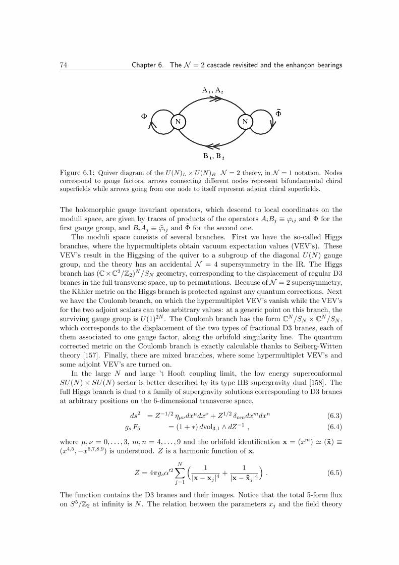
74 Chapter 6. The N = 2 cascade revisited and the enhancon bearings
Figure 6.1: Quiver diagram of the U(N)L × U(N)R N = 2 theory, in N = 1 notation. Nodescorrespond to gauge factors, arrows connecting different nodes represent bifundamental chiralsuperfields while arrows going from one node to itself represent adjoint chiral superfields.
The holomorphic gauge invariant operators, which descend to local coordinates on themoduli space, are given by traces of products of the operators AiBj ≡ ϕij and Φ for thefirst gauge group, and BiAj ≡ ϕij and Φ for the second one.
The moduli space consists of several branches. First we have the so-called Higgsbranches, where the hypermultiplets obtain vacuum expectation values (VEV’s). TheseVEV’s result in the Higgsing of the quiver to a subgroup of the diagonal U(N) gaugegroup, and the theory has an accidental N = 4 supersymmetry in the IR. The Higgsbranch has (C×C
2/Z2)N/SN geometry, corresponding to the displacement of regular D3
branes in the full transverse space, up to permutations. Because ofN = 2 supersymmetry,the Kahler metric on the Higgs branch is protected against any quantum corrections. Nextwe have the Coulomb branch, on which the hypermultiplet VEV’s vanish while the VEV’sfor the two adjoint scalars can take arbitrary values: at a generic point on this branch, thesurviving gauge group is U(1)2N . The Coulomb branch has the form C
N/SN × CN/SN ,
which corresponds to the displacement of the two types of fractional D3 branes, each ofthem associated to one gauge factor, along the orbifold singularity line. The quantumcorrected metric on the Coulomb branch is exactly calculable thanks to Seiberg-Wittentheory [157]. Finally, there are mixed branches, where some hypermultiplet VEV’s andsome adjoint VEV’s are turned on.
In the large N and large ’t Hooft coupling limit, the low energy superconformalSU(N)× SU(N) sector is better described by its type IIB supergravity dual [158]. Thefull Higgs branch is dual to a family of supergravity solutions corresponding to D3 branesat arbitrary positions on the 6-dimensional transverse space,
ds2 = Z−1/2 ηµνdxµdxν + Z1/2 δnmdx
mdxn (6.3)
gs F5 = (1 + ∗) dvol3,1 ∧ dZ−1 , (6.4)
where µ, ν = 0, . . . , 3, m,n = 4, . . . , 9 and the orbifold identification x = (xm) ≃ (x) ≡(x4,5,−x6,7,8,9) is understood. Z is a harmonic function of x,
Z = 4πgsα′2
N∑
j=1
( 1
|x− xj |4+
1
|x− xj |4)
. (6.5)
The function contains the D3 branes and their images. Notice that the total 5-form fluxon S5/Z2 at infinity is N . The relation between the parameters xj and the field theory

6.2. D3 branes on the C2/Z2 orbifold and a cascading solution 75
moduli is xj = 2πα′φj , where φj is an eigenvalue of the VEV of some field. Φ and Φ aremapped to x4+ix5, while ϕij are mapped to algebraic coordinates zij on C
2/Z2, such thatz12z21 − z211 = 0 and z22 = z11. The supergravity axio-dilaton τ = C0 + i e−Φ = C0 +
igs
is constant,1 as D3 branes do not couple to it. It is related to the field theory gaugecouplings and theta angles by
τ = τ1 + τ2 where τj =θj2π
+4πi
g2j, j = 1, 2 . (6.6)
In the following we will take τ = i/gs unless otherwise stated.As noticed in [134], for a generic point on the Higgs branch (and more generally on any
branch), the supergravity solution has large curvature. However, configurations whereall the branes are in big clumps have a good supergravity description, and configurationswhere only a small number of branes are isolated are well described by probe branes inthe background generated by the other branes.
The Coulomb branch of our N = 2 quiver is described by fractional D3 branes alongthe orbifold singularity. In this case supergravity solutions include a non-trivial profilefor the twisted field fluxes. Indeed, fractional D3 branes source magnetically the twistedscalar c and by supersymmetry they also source its NSNS partner, the twisted scalarb. This can be easily understood recalling [41] that fractional D3 branes are D5 braneswrapped on the exceptional 2-cycle C which lives at the orbifold singularity. The twistedscalars are simply the reduction of the RR and NSNS 2-form potentials, C2 and B2, onC. They can be organized in a complex field as
γ ≡ c+ τb = c+i
gsb =
1
4π2α′
∫
C
(
C2 +i
gsB2
)
, (6.7)
while
G3 = F3 +i
gsH3 = 4π2α′ dγ ∧ ω2 (6.8)
is the complexified 3-form field strength, where ω2 is a closed anti-selfdual (1, 1)-form withdelta-function support at the orbifold plane, normalized as
∫
C ω2 = 1. Regular D3 branesdo not couple to the twisted sector, hence the profile of γ is affected solely by fractionalbranes. The complex twisted scalar γ is then subject to a two-dimensional Laplaceequation in C with sources at the positions of the fractional branes. Supersymmetricsolutions [123] have primitive, imaginary self-dual and (2, 1) G3 flux, which implies thatγ = γ(z) is a meromorphic function of z = x4 + ix5, such that dγ(z) has simple polesat the locations of sources. For a bunch of N fractional and N anti-fractional2 branes atpositions zj and zj , respectively, we have
γ =i
π
[ N∑
j=1
log(z − zj)−N∑
j=1
log(z − zj)]
+ γ(0) . (6.9)
1We work in the string frame. Here Φ is the full dilaton, which is constant in all the solutions underconsideration, not to be confused with one of the adjoint chiral superfields. From now on we will ratheruse gs = eΦ.
2With some abuse of language, following [152] we call ‘anti-fractional branes’ D5 branes wrapped onC with the opposite orientation, with some worldvolume flux through C in order to preserve the samesupercharges as the fractional branes.
76 Chapter 6. The N = 2 cascade revisited and the enhancon bearings
Here γ(0) is an integration constant: its imaginary part sets the value of b at large |z|or in the theory at the origin of the moduli space, while the real part does not reallyhave a physical meaning in the dual theory because of the presence of the axial anomaly,and we will set it to zero. The positions of the fractional branes zj and zj are classicallyidentified with the eigenvalues Φj , Φj of the field theory adjoint scalars. Corrections tothis identification arise at quantum level and will be discussed in the next section.
The holographic relations between the Yang-Mills couplings and theta angles and thesupergravity fields are
τ1 + τ2 = τ τ1 − τ2 = 2γ − τ = 2[
c+ τ(
b− 1
2
)]
, (6.10)
but we will often set τ = i/gs. In particular, when b = 0 the imaginary part of τ1 vanishesand g1 diverges, whereas for b = 1 it is g2 which diverges.3 What we face in such casesis obviously a peculiar field theory, a SCFT with one divergent gauge coupling, in whichinstanton corrections dominate even in the large N limit [159], and about which not muchis known. Although from the Seiberg-Witten curve analysis one does not expect extramassless fields in general, the supergravity description is a very incomplete descriptionfor this phase. When c ∈ Z as well, extra massless states do appear, and the theory entersa tensionless string phase, as originally suggested in [160] from consistency of T -dualitywith type IIA string theory.
So far, we have only discussed the superconformal SU(N)×SU(N) theory,4 which hasa well behaved UV limit and whose stringy realization through AdS/CFT is unambiguous.However, what we are really interested in is the non-conformal SU(N +M) × SU(N)gauge theory. This can be easily obtained through Higgsing from the superconformalSU(N +M)× SU(N +M) theory, which can be engineered placing N +M regular D3branes at the origin of the orbifold: takingM VEV’s of the second adjoint scalar to be ata scale |z0|/2πα′ produces an effective SU(N +M)×SU(N)×U(1)M theory below |z0|,5where the U(1) factors are IR free and decouple. In the dual picture, this correspondsto placing M anti-fractional branes at, say, the roots of zMj = −zM0 , while the otherN anti-fractional branes and N +M fractional branes sit classically at the origin. Thetwisted scalar in this configuration is then
γ =i
πlog
zM
zM + zM0+ γ(0) . (6.11)
For the sake of simplicity, unless differently specified, in the following we will set theorbifold point value γ(0) = i
2gs[161, 162], so that in the UV τ1 = τ2 = i
2gs. In the large
M limit in which we work, (6.11) can be traded for its limiting behavior
γ =
i Mπ log zz0
+ i2gs≡ i Mπ log z
z1if |z| < |z0|
γ(0) if |z| > |z0|(6.12)
3Actually b ∈ [0, 1] is the only range of validity of the formulas, because otherwise one would havenegative square couplings. As noticed in [118] and extensively discussed in [129, 1], when b is outsidethis range one has to perform a large gauge transformation to shift it to the interval where (6.10) can beapplied.
4From now on, we will often consciously forget the additional U(1) × U(1) factor which decouples atlow energies.
5In the following, when speaking about scales we will often omit the 2πα′ factor.

6.3. The enhancon and the Seiberg-Witten curve 77
where we set z1 = eiπMγ(0) z0 = e
− π2gsM z0. Note that the twisted fluxes break the U(1)
isometry corresponding to rotation in the z-plane to a discrete subgroup Z2M6. This is
dual to the breaking of the U(1) R-symmetry because of anomalies in the gauge theory[163].
The gauge invariant D3 brane charge (Maxwell charge) carried by the fluxes of thesolution is proportional to the 5-form flux; it is found by integrating the Bianchi identityin the absence of sources dF5 = −H3 ∧ F3 on the angular S5/Z2 of radius r and reads,for r < ρ0 = |z0|,
− 1
(4π2α′)2
∫
F5 = N +gsM
2
πlog
r
ρ1(6.13)
with ρ1 = |z1|.We see from eqs.(6.12)-(6.13) that, similarly to the Klebanov-Tseytlin (KT) solution
[127], the solution enjoys logarithmically varying B field and 5-form flux below the cutoff:this naturally suggests that the dual field theory might enjoy a cascading RG flow withsubsequent infinite coupling transitions reducing the rank of the infinitely coupled non-
abelian gauge group by 2M at scales ρk = e− (2k−1)π
2gsM ρ0, k = 1, . . . , l, where l ≡ [N/M ]−7
[11]. This will be dealt with in section 4, where the N = 2 cascading nature of thesolution will be discussed in great detail.
Before attacking this problem, though, we have to deal with another phenomenon,which always arises in supergravity solutions dual to non-conformal supersymmetric gaugetheories with eight supercharges. By analyzing the explicit form of the warp factor, itwas shown in [10] that the ten-dimensional metric obtained using (6.11), besides theobvious singularity on the orbifold fixed plane, displays an unphysical repulsive regionnear the origin, at a scale of order e−πN/gsM
2ρ1.
8 One expects that, as suggested in [10],an enhancon-like mechanism [156] might be at work here, which excises the unphysicalregion rendering back a repulson-free solution. We will show that this is indeed the case,discussing in the next section the specific way in which the enhancon mechanism manifestsin this context, and providing in section 6.6 an excised and singularity-free solution.
6.3 The enhancon and the Seiberg-Witten curve
The quantum corrections to the Coulomb branch constrain the (anti)fractional D3 branepositions, zj and zj , in the gravity dual. The full quantum corrected moduli space isexactly encoded in the full family of Seiberg-Witten (SW) curves [80, 154]. The SWcurves for the N = 2 superconformal field theory at hand were found in [157]. At theclassical level, the fractional brane positions zj and zj correspond to the eigenvalues of theVEV’s of the adjoint scalars Φ and Φ. In the quantum theory this identification cannotsurvive because the VEV’s parametrize the moduli space and are unconstrained, whereasfractional brane positions are constrained. That is, in the large N limit one expects [134]quantum corrections and the consequent constraints on zj and zj to be bound, because
6Really, the cutoff fractional branes only preserve ZM , but this is irrelevant at large M or not veryclose to those branes.
7We denote by [y]± the ceiling and floor functions, namely the integers which better approximate yfrom above and below respectively.
8See appendix A of [164] for an analytic study of the warp factor found in [10].

78 Chapter 6. The N = 2 cascade revisited and the enhancon bearings
of supersymmetry, to a non-negative 5-form flux (that means non-negative enclosed D3-charge) for all allowed configurations on the quantum moduli space, at least whenever thesupergravity approximation is valid. This property is in fact at the core of the enhanconmechanism.
Let us detail this point by first considering a simplified example. Consider the theorydiscussed previously with N = 0: this is an SU(M) × SU(M) superconformal theorywhich can be engineered by M regular D3 branes. Below the UV scale |z| = |z0|, thetheory is effectively Higgsed to SU(M) N = 2 pure SYM (plus IR free U(1) factors).The dual supergravity solution is the one in (6.12)-(6.13) with N = 0, and it correspondsto the M fractional branes classically at the origin. The quantum moduli space can bestudied with a good approximation by means of the SW curves for SU(M) [165, 166]
y2 =
M∏
a=1
(v − φa)2 + 4Λ2M , (6.14)
where Λ is the strong coupling scale of N = 2 SU(M) SYM and φa are the eigenvaluesof the adjoint scalar Φ parametrizing a family of hyperelliptic curves in C
2 = (v, y).The curves could also be written in terms of gauge invariant symmetric polynomials.Classically (Λ = 0) the eigenvalues φa coincide with the double branch points of (6.14),and correspond to the fractional brane positions on the z plane in the gravity description.An elegant way to see this is the following: type IIB string theory on the orbifold is T-dual to type IIA on a circle (with coordinate x6) with two parallel NS5 branes alongx0, · · · , x5, separated in the compact direction x6 (see [167] for a review). Fractional D3branes are T-dual to D4 branes stretched along x6 between the two NS5’s. The classicalCoulomb branch is then given by all the possible configurations of D4 branes on theplane v = x4 + ix5. The system can be further uplifted to M-theory, where the NS5’sand the D4’s are just part of a single M5 brane. The M5 brane seen as a Riemannsurface is identified with the SW curve [157]. At the quantum level, the eigenvalues φastill parametrize the whole moduli space (up to Weyl gauge identifications), but theyno longer correspond to double branch points nor fractional brane positions, strictlyspeaking. In the perturbative regime of the theory, |φa| ≫ |Λ|, the branch points stillappear in pairs close to φa: in the M-theory picture the D4 branes are inflated into smalltubes. As soon as the VEV’s get into the non-perturbative region (at scales comparablewith Λ), the branch points get well separated and it does not make much sense to talkabout fractional brane positions anymore.
At the origin of the moduli space (Φ = 0), the hyperelliptic curve (6.14) becomesy2 = v2M + 4Λ2M , which has 2M separate branch points at v2M = −4Λ2M . In the largeM limit, the branch points densely fill a ring of radius 21/M |Λ|. It is also possible tosee that, adding a probe fractional brane (in field theory terms, consider the SU(M + 1)theory with one additional VEV φ), in which case the SW curves are
y2 = v2M (v − φ)2 + 4Λ2M+2 , (6.15)
the probe can freely move in the semi-classical region outside the ring, but it cannotpenetrate it. For |φ| ≫ |Λ|, the two extra branch points are placed near φ, with a smallseparation of order Λ(Λ/φ)M , while the other 2M branch points are still on the ring. As|φ| approaches |Λ| and then goes to zero, the branch points split and melt into the ring.
6.3. The enhancon and the Seiberg-Witten curve 79
As anticipated, the dual string theory picture of this is the famous enhancon mech-anism [156]. The tension of BPS fractional D3 branes is equal to their gauge invariantMaxwell D3-charge, which is γ
Tnf =µ3gs
∣∣gs Im γ + nf
∣∣ =
µ3gs
∣∣b+ nf
∣∣ , (6.16)
where nf is the number of units of worldvolume flux on the exceptional 2-cycle C (noticethat neither b or nf are gauge invariant, while their sum is). This turns out to beproportional to the perturbative moduli space metric on the Coulomb branch of theSU(M) N = 2 pure SYM theory9 [10]. At the scale |Λ| = ρ1, b vanishes and fractionalD3 branes, which are wrapped D5 branes with no worldvolume flux, become tensionless;below that scale they would be non-supersymmetric and they would feel a repulsivepotential. Notice also that the enclosed D3 brane charge would become negative forsmaller scales, which could hardly be the case if fractional D3 branes were at the origin.Moreover, a massive particle probe would experience an unphysical gravitational repulsionclose to the origin. The resolution of this puzzle is that fractional branes cannot bebrought all at the same place, but rather melt into a thin ring of radius ρ1: the enhanconring. This changes the twisted fields distribution in the geometry: inside the ring, b = 0(more generally it is integer), c is constant, and there is no D3 brane charge. The warpfactor needs to be re-computed using the correct configuration of fractional branes andtwisted field, and the result is that the suspicious repulsive region disappears, as will beshown in section 6.6.
In some sense, the whole region defined by b = 0 (more generally b ∈ Z) behaveslike a conductor: D5 charges (recall that the D3 charge vanishes along with the tensioninside the enhancon) are pushed to the boundary and there is no field inside. We will callsuch a region the enhancon plasma. We already noticed in section 6.2 that the IR fieldtheory dual to the interior region is quite peculiar: it is a conformal SU(N) × SU(N)theory with one divergent gauge coupling. However, in this particular case N = 0 and thedynamics is trivial inside the enhancon plasma: SU(M) is simply broken by instantonsto U(1)M−1.
As discussed in [152], exactly the same kind of behavior can be found in the mostgeneric situation, i.e. when N 6= 0 and the theory has product gauge group SU(N+M)×SU(N). Since the second gauge group is not asymptotically free, one should embed thetheory into the SU(N+M)×SU(N+M) conformal one, properly Higgsed, as sketched atthe end of Section 6.2. One can then exploit the power of the Seiberg-Witten technology.In order to write down the SW curve, let us define the complex coordinate
u = ix6 + ix10
2πR10, (6.17)
which parametrizes the M-theory torus defined by the identifications u ≃ u+ 1 ≃ u+ τ .The complex structure τ is identified with the type IIB axio-dilaton. Let us also definethe parameter q = e2πiτ and the coordinate t = e2πiu; note that t ≃ qt on the torus.
9There is a matching with the perturbative result because in the large M limit instanton correctionsare strongly suppressed, and abruptly show up at the scale Λ [159].

80 Chapter 6. The N = 2 cascade revisited and the enhancon bearings
For concreteness, let us stick again to the case of equal gauge couplings in the UVCFT: τ1 = τ2 = τ/2. In terms of the quasi-modular Jacobi θ-functions
θ2(2u|2τ) =∞∑
n=−∞
q(n−12)2t2n−1 (6.18)
θ3(2u|2τ) =∞∑
n=−∞
qn2t2n , θ4(2u|2τ) =
∞∑
n=−∞
(−1)nqn2t2n , (6.19)
the SW curve for the conformal theory can be written as [168]
S(v) +R(v)
S(v)−R(v) = f(u|τ), with f(u|τ) ≡ θ3(u|τ/2)θ4(u|τ/2)
=θ3(2u|2τ) + θ2(2u|2τ)θ3(2u|2τ)− θ2(2u|2τ)
, (6.20)
or alternatively
R(v)
S(v)= g(u|τ), with g(u|τ) ≡ f − 1
f + 1=θ2(2u|2τ)θ3(2u|2τ)
. (6.21)
Here R(v) =∏N+Ma=1 (v − φa) and S(v) =
∏N+Ma=1 (v − φa) are degree N +M polynomials
whose zeros φa and φa are the eigenvalues for the adjoint scalars of the first and secondgauge group, respectively.
Following [152], let us choose a ZM -invariant configuration for the anti-fractionalbranes Higgsing the CFT at large |z| (i.e. large |v| for the corresponding D4 branes), andconsider the origin of the moduli space of the low energy SU(N +M)× SU(N) theory,
R(v) = vN+M S(v) = vN (vM − zM0 ) . (6.22)
The N common zeros of R(v) and S(v) factor out of the curve, without affecting the RGflow. They correspond to N D3 branes, whose moduli space is flat (apart from orbifoldsingularities when several branes coincide) and not quantum corrected. We are then leftto consider an SU(M)× SU(M) theory, spontaneously broken to SU(M)× U(1)M−1 atthe scale z0. Hence, if the IR dynamics is not much affected by the UV Higgsing, as it isnatural to expect, the low energy physics should be similar to the enhancon mechanismpreviously discussed, but with N leftover regular D3 branes.
Let us give further evidence for the above claim. As explained in [157], we can extractthe running of the gauge coupling from the bending of the two NS5 branes due to theunbalanced D4 branes tension. In the M-theory picture, the gauge couplings at a scalev can be extracted from the SW curve looking at the corresponding two values of u; wehave that
∆u = τ1, τ −∆u = τ2 , (6.23)
while the map between the type IIB twisted scalars (c, b) and the field theory couplings(τ1, τ2) was given in (6.10). In particular, the curve (6.20) at the point (6.22) on theCoulomb branch reads
1− 2( v
z0
)M= f(u|τ) . (6.24)
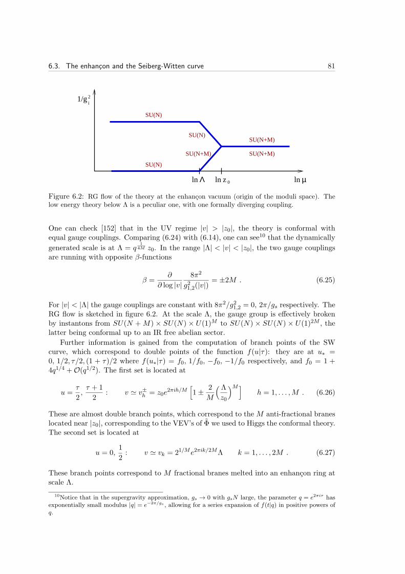
6.3. The enhancon and the Seiberg-Witten curve 81
1/gi2
SU(N+M)
SU(N+M)
SU(N)
SU(N)
µln
SU(N)
SU(N+M)
lnln Λ 0z
Figure 6.2: RG flow of the theory at the enhancon vacuum (origin of the moduli space). Thelow energy theory below Λ is a peculiar one, with one formally diverging coupling.
One can check [152] that in the UV regime |v| > |z0|, the theory is conformal withequal gauge couplings. Comparing (6.24) with (6.14), one can see10 that the dynamically
generated scale is at Λ = q1
4M z0. In the range |Λ| < |v| < |z0|, the two gauge couplingsare running with opposite β-functions
β =∂
∂ log |v|8π2
g21,2(|v|)= ±2M . (6.25)
For |v| < |Λ| the gauge couplings are constant with 8π2/g21,2 = 0, 2π/gs respectively. TheRG flow is sketched in figure 6.2. At the scale Λ, the gauge group is effectively brokenby instantons from SU(N +M) × SU(N) × U(1)M to SU(N) × SU(N) × U(1)2M , thelatter being conformal up to an IR free abelian sector.
Further information is gained from the computation of branch points of the SWcurve, which correspond to double points of the function f(u|τ): they are at u∗ =0, 1/2, τ/2, (1 + τ)/2 where f(u∗|τ) = f0, 1/f0, −f0, −1/f0 respectively, and f0 = 1 +4q1/4 +O(q1/2). The first set is located at
u =τ
2,τ + 1
2: v ≃ v±h = z0e
2πih/M[
1± 2
M
( Λ
z0
)M]
h = 1, . . . ,M . (6.26)
These are almost double branch points, which correspond to theM anti-fractional braneslocated near |z0|, corresponding to the VEV’s of Φ we used to Higgs the conformal theory.The second set is located at
u = 0,1
2: v ≃ vk = 21/Me2πik/2MΛ k = 1, . . . , 2M . (6.27)
These branch points correspond to M fractional branes melted into an enhancon ring atscale Λ.
10Notice that in the supergravity approximation, gs → 0 with gsN large, the parameter q = e2πiτ hasexponentially small modulus |q| = e−2π/gs , allowing for a series expansion of f(t|q) in positive powers ofq.
82 Chapter 6. The N = 2 cascade revisited and the enhancon bearings
As in the pure SYM case, probe fractional branes can be studied on this backgroundby means of the SW curves for the SU(N +M + 1)× SU(N +M + 1) theory
R(v)
S(v)=
vM (v − φ)(vM − zM0 )(v − φ)
= g(u|τ) , (6.28)
where φ and φ parametrize the extra VEV for Φ and Φ. The branch points correspondingto the eigenvalue φ (the fractional D3 probe) can freely move outside the enhancon ring,but as they approach it and φ goes to 0, the two branch points split and melt intothe enhancon ring. The two branch points corresponding to the eigenvalue φ (the anti-fractional D3 probe) can instead penetrate the enhancon ring; when this happens, theyunchain two branch points from the ring which follow them inside: an anti-fractionalbrane eats a melted fractional brane from the ring, forming a regular D3 brane free tomove everywhere.
From this analysis, one concludes that, no matter the value of N , the fluxes in eqs.(6.12) and (6.13) do describe the physics of the SU(N+M)×SU(N) theory at the originof its moduli space, provided that they are excised at radius ρ1 ≃ |Λ| by an enhanconmechanism. The solution should also be cut off at a radius |z0|, or completed with Manti-fractional branes, providing a conformal AdS5 UV completion. As already stressed,the warp factor needs to be recomputed in the presence of the correct configuration offractional branes and excised twisted fields. This will be done in section 6.6.
Notice, however, that the supergravity solution of eqs. (6.12) and (6.13) does not
seem to have any pathology below ρ1, at least down to a scale of order e− πNgsM2 ρ1, where
the 5-form flux (6.13) vanishes and the problematic repulsive region starts. The questionarises whether there is any field theory interpretation for such a solution, suitably excisedonly at a radius
ρmin = ρl+1 ≡ e−πlgsM ρ1 with l ≡ [N/M ]−, (6.29)
the smallest infinite coupling scale outside the region of negative D3 brane charge. Asalready noticed, the presence of a constant 3-form flux and the logarithmic running of the5-form flux strongly suggests a cascading behavior, as for the Klebanov-Tseytlin-StrasslerN = 1 model [118, 127], properly adapted to a N = 2 setting. An interpretation of thewould-be N = 2 RG flow that can be extracted from the supergravity solution in termsof some sort of Seiberg duality cascade was in fact argued for in [11], but the existenceof an appropriate N = 2 duality had not been clarified, so far. On the other hand, in[134] the reduction of 5-form flux was interpreted as due to a distribution of D3 branesand/or wrapped D5 branes. It was further suggested that a suitable distribution of D3branes only (Higgs branch) could perhaps account for it. However, the latter proposalencounters some problems in reproducing the running of gauge couplings and decrease ofnonabelian gauge group ranks that is suggested by the supergravity solution.
Drawing on well established results about N = 2 SQCD, we propose that there existfield theory vacua, not at the origin of the Coulomb branch, which display a cascadingbehavior. They are dual to the solution in (6.12) and (6.13), valid well below the firstinfinite coupling radius ρ1 down to some much lower scale, at most until the so-calledtrue enhancon scale Λmin = ρmin, where the twisted fields are excised. ρmin is named
6.4. The cascading vacuum in field theory 83
the true enhancon radius since it is the scale at which the excision is performed. All thehigher infinite coupling scales, ρj with j = 1, . . . , l, will be called generalized enhanconradii [134].
We provide a precise identification of these vacua in the next section. The excisionof the twisted fields by means of the enhancon mechanism and the disappearance of thenaive singularity will be discussed in section 6.6. Depending on the field theory vacuaone is studying, the excision can take place at different scales, for instance at ρ = ρ1,as in the vacua discussed in this section, or at the bottom of the cascade, at the scaleρ = ρmin, as for the cascading vacua to be discussed in section 4.
6.4 The cascading vacuum in field theory
The perturbative RG flow of the SU(N +M) × SU(N) theory, given in (6.25), is suchthat the largest group goes to strong coupling at a scale Λ. The supergravity solution weare considering suggests that, in the dual vacuum, a mechanism effectively reduces thegauge group to SU(N−M)×SU(N) below Λ, plus possible U(1) factors. This statementcan be supported by a computation of Page charges in supergravity, in the gauge thatgives sensible field theory couplings (as extensively discussed in [129, 1]). The value of b,in the gauge in which b ∈ [0, 1], is found from (6.12) to be
b = gs Im γ =gsM
πlog
ρ
ρ1−[gsM
πlog
ρ
ρ1
]
−, (6.30)
where ρ = |z|. The D5 and D3 brane Page charges at radius r are evaluated to be11
QPage5 = − 1
4π2α′
∫F3 = 2M (6.31)
QPage3 = − 1
(4π2α′)2
∫(F5 +B2 ∧ F3) = N +M
[gsMπ log r
ρe
]
−. (6.32)
This shows that the non-abelian factors in the gauge group drop as SU(N + M) ×SU(N)→ SU(N −M)×SU(N) not only at the first strong coupling scale ρ1 = Λ1 ≡ Λ,but actually at each generalized enhancon, which occurs at a scale
ρk = Λk = e−π(k−1)
gsM Λ1 = e−π(2k−1)
2gsM ρ0 k = 1, . . . , l , (6.33)
where recall that l = [N/M ]− and we also set N = lM + p. Finally, at Λl+1 ≡ Λmin ≡e− πlgsM Λ1 there is a true enhancon ring with M tensionless fractional branes, and the
non-abelian factors in the gauge group reduce according to SU(M + p) × SU(p) →SU(p)×SU(p), with one infinite gauge coupling. Twisted fields have to be excised thereso as to avoid negative D3-charge in the interior region.
In passing let us stress, as in [134], that even though their dynamics takes place atarbitrarily low energies, the possible additional U(1) factors are described in the holo-graphic setup by modes at a finite radius where the corresponding fractional D3 braneslie.
11The 3-cycle where the D5 charge integration is performed is the product of the exceptional 2-cycle Cand an S1 on the orbifold line. Since the intersection number is (D, C) = −2 where D is the cone overthe 3-cycle, the D5 charge is twice the number of wrapped D5 branes.

84 Chapter 6. The N = 2 cascade revisited and the enhancon bearings
In order to have an intuition on the strong coupling dynamics at hand, let us firstfocus on the first such generalized enhancon, which occurs at the scale Λ1 = Λ. This willclearly be a prototype for any generalized enhancons. As already stressed, at the scale Λ,the coupling of the largest gauge group diverges (and instantonic corrections dominate),while the other gauge coupling reaches the value g2min = 4πgs. As a first step towardthe understanding of the precise mechanism taking place, we can consider a corner ofthe parameter space of the gauge theory where Ng2min → 0. In this limit, the gaugedynamics of the second factor decouples and it effectively becomes a global symmetry:the theory around Λ is simply SU(N +M) SQCD with 2N flavors. Moreover, possibleVEV’s for the smaller group adjoint scalar effectively behave as masses for the largergroup hypermultiplets. In this case we are out of the supergravity approximation butthis analysis will give us some good insight. Hence, let us quickly review some resultsabout the moduli space of N = 2 SQCD.
6.4.1 One cascade step: N = 2 SQCD
The moduli space of N = 2 SQCD [155] with Nc colors and Nf flavors consists ofa Coulomb branch and of various Higgs branches. The Coulomb branch [169, 155] isparametrized by the vacuum expectation value of the adjoint scalar field Φ in the N = 2vector multiplet,
Φ = Diag(φ1, . . . , φNc)∑
a
φa = 0 , (6.34)
and is thus given by the Nc − 1 dimensional complex space of φa’s modulo permuta-tions (Weyl gauge transformations). The VEV’s generically break the SU(Nc) gaugegroup to its Cartan subgroup U(1)Nc−1. However, at special submanifolds where theHiggs branches meet the Coulomb branch a non-abelian gauge symmetry survives. Higgsbranches can be divided into a baryonic branch and various non-baryonic branches (ac-cording to whether baryonic operators acquire VEV’s or not); the corresponding inter-sections with the Coulomb branch were dubbed roots.12 Higgs branches are not quantumcorrected, however their intersections among themselves and with the Coulomb branchare modified at quantum level.
The SW curve describing the Coulomb branch for vanishing masses is [169, 171]
y2 =
Nc∏
a=1
(x− φa)2 + 4Λ2Nc−NfxNf . (6.35)
Nonbaryonic branches are labeled by an integer 1 ≤ r ≤ min([Nf/2]−, Nc − 2). The lowenergy effective theory at the roots are the IR free or finite SU(r) × U(1)Nc−r SQCDwith Nf hypermultiplets in the fundamental representation and charged under one ofthe U(1) factors. At special points along these submanifolds, the SW curve shows thatNc − r − 1 additional massless singlet hypermultiplets arise, each one charged under oneof the remaining U(1) factors. It is important that there are 2Nc−Nf such vacua, relatedby the broken Z2Nc−Nf non-anomalous R-symmetry acting on the Coulomb branch.
12Issues related to the baryonic root of N = 2 SQCD and the mass deformation to N = 1 were recentlydiscussed in [170].

6.4. The cascading vacuum in field theory 85
The baryonic branch exists for Nc ≤ Nf , and the baryonic root is a single point,invariant under the Z2Nc−Nf R-symmetry. Thus its coordinates on the Coulomb branchare13
Φbb = (0, . . . , 0︸ ︷︷ ︸
Nf−Nc
, φ ω, φω2, . . . , φ ω2Nc−Nf ) , (6.36)
where ω = exp2πi/(2Nc −Nf ), for some value of φ (and φ = 0 classically). The gaugegroup is thus broken to SU(Nf −Nc)×U(1)2Nc−Nf , which is IR free.14 The requirementthat a Higgs branch originates from this root implies the presence of 2Nc −Nf masslesshypermultiplets charged only under the U(1) factors; this singles out a point in thesubmanifold described by (6.36). The result is φ = Λ, so that the SW curve takes thesingular form
y2 = x2(Nf−Nc)(x2Nc−Nf + Λ2Nc−Nf
)2. (6.37)
The x2(Nf−Nc) factor corresponds to an unbroken SU(Nf − Nc) gauge group. The re-
maining 2(2Nc −Nf ) branch points show up in coincident pairs, located at xk = Λωk−12
with k = 1, . . . , 2Nc−Nf , corresponding to the 2Nc−Nf mutually local massless hyper-multiplets.
The reason for this detour should be clear by now: the non-perturbative dynamics atthe baryonic root preserves the same Z2Nc−Nf = Z2M R-symmetry as the supergravitysolution we are discussing, and its low energy effective theory possesses an SU(Nf −Nc) = SU(N −M) non-abelian gauge symmetry precisely matching the numerology ofthe cascading interpretation. Hence, iterating the above procedure at the subsequentgeneralized enhancons Λk (where the higher rank gauge group coupling diverges), it isnatural to propose the supergravity solution in (6.12) and (6.13) (excised only down atthe true enhancon ρmin) to be dual to a cascading SU(N +M) × SU(N) quiver gaugetheory at subsequent baryonic roots of the strongly coupled gauge groups.15 In whatfollows, we will provide several checks for the validity of our proposal.
6.4.2 The cascading vacuum in the quiver gauge theory
Let us now turn to the full quiver gauge theory SU(N +M)× SU(N). The vacuum wepropose as the dual of the full cascading solution is a vacuum in which, at each step alongthe resulting cascade, the largest of the two gauge groups goes to strong coupling witha behavior analogous to the the baryonic root of SQCD. This vacuum is invariant underthe same non-anomalous Z2M subgroup of the R-symmetry as the supergravity solutionwe started with. Moreover, not only has it the correct spontaneous symmetry breakingpattern but also the correct RG flow, including the beta functions and the separation ofscales where the transitions occur, as can be extracted from supergravity.
It is worth stressing that our vacuum does not sit exactly at the baryonic roots, asthere are no baryonic roots in the quiver theory (see section 6.4.4 for an exception).
13For Nf > 3Nc/2 there are other Z2Nc−Nf-invariant submanifolds. However the baryonic root is just
one point, and one can show that it in fact belongs to the submanifold (6.36) [155].14We assume Nf < 2Nc so that the microscopic theory is UV free. This bound is satisfied in the
cascading quiver theory.15We should mention that a proposal for an N = 2 cascade at the baryonic root has been alluded to in
[172], in the context of the M-theory realization of this elliptic model.

86 Chapter 6. The N = 2 cascade revisited and the enhancon bearings
However, it does approximate them in the supergravity limit in which q → 0, which isthe limit of interest to us.
Let us start for concreteness with an SU((2K + 1)M) × SU((2K + 1)M) conformaltheory in the UV and then break the gauge group to SU((2K + 1)M) × SU(2KM)by giving VEV’s of order z0 in a ZM -invariant way to M eigenvalues of the adjointscalar Φ. We choose a vacuum in which, at each step of the RG flow, the most stronglycoupled group is at its baryonic root (in the q → 0 limit). Let us write the SW curveas R(v)/S(v) = g(u|τ) as in (6.21), where u is the coordinate on a torus of complexstructure τ . We choose the polynomials R(v) and S(v) of degree (2K + 1)M , as
R(v) = vMK−1∏
j=0
(v2M + q12+2j z2M0 )
S(v) = (vM − zM0 )K−1∏
j=0
(v2M + q32+2j z2M0 ) .
(6.38)
The polynomial R(v) is related to the SU((2K + 1)M) group that starts flowing to-ward strong coupling at the cutoff scale z0, whereas the polynomial S(v) is related tothe SU((2K + 1)M) group which is spontaneously broken to SU(2KM) there.16 Theeigenvalues of the two adjoint scalar fields are put, in an alternating manner, at energiescorresponding to their subsequent strong coupling scales along the cascade: in the limitin which the dynamics of the weakly coupled group decouples at those scales, the vacuamimic the SQCD baryonic root. In agreement with the cascading RG flow of the super-gravity solution, the hierarchy of strong coupling scales is controlled by q = e2πiτ . Becauseof the large M limit, the running is led by the perturbative beta functions except at thesuccessive strong coupling scales, where instantonic corrections sharply appear. This fieldtheory running can be explicitly checked either numerically using the exact SW curve wewrote, or analytically by expanding the polynomials energy range by energy range, in aneffective field theory approach (see Appendix E.7). A plot of the resulting RG flow isshown in figure 6.3.
We now move on to the study of the branch points of the curve. Recall that branchpoints are double solutions in v at fixed u. In the dual type IIA construction, a pairof coincident branch points at v corresponds to a D4 brane stretched between the twoNS5’s, while in type IIB it corresponds to a fractional brane at position z ≃ v on theorbifold singularity line. When the branch points are not in pairs, the full M-theorydescription is needed, fractional branes are no longer perturbative states in type IIB andtheir wavefunction is spread over the whole b ∈ Z region [156] (at least in the large Mlimit).
It turns out that the branch points for u = 0, 1/2, up to corrections of higher orderin q, lie at
vM ≃ ∓qn+1/4 zM0 , n = 0, . . . ,K − 1 and vM ≃ ∓2qK+1/4 zM0 . (6.39)
16Very similarly, we can also describe a cascade with an SU(2KM) × SU(2KM) UV completion: itamounts to putting the cutoff and the vanishing eigenvalues in the same adjoint field/polynomial in(6.38), otherwise preserving the structure of the polynomials. Finally, the generalization to the cascadewith N = lM + p can be achieved by multiplying R and S by the same degree p polynomial.

6.4. The cascading vacuum in field theory 87
1/gi2
N+M
N+M
Λ 0z
N+M
1
N−M
NN
N−2M
N−M
Λ 2lΛΛ l +1
M+p
p
2M+p
M+p
p
p
µ
Figure 6.3: RG flow of the theory at the cascading vacuum (taking p = 0, for definiteness). Here,as well as in figures 6.4 and 6.6, the horizontal axis is logarithmic and we have omitted the SUfactors for the gauge groups, to avoid clutter.
The former class of points consists of K sets of 2M double points (which are doubleup to an accuracy discussed at the end of the next subsection), corresponding to theK baryonic-root-like VEV’s of the first gauge group, whereas the latter are 2M wellseparated branch points, corresponding to the true enhancon of the low energy SU(M)theory. The branch points for u = τ/2, (τ + 1)/2 lie at
vM = ∓qn+3/4 zM0 , n = 0, . . . ,K − 1 and vM = (1± 2q1/4) zM0 . (6.40)
The first class of points consists again of K sets of 2M (almost) double points, corre-sponding to the K baryonic-root-like VEV’s of the second gauge group, while the secondset of points are the almost paired branch points associated to semiclassical fractionalbranes at the cutoff scale z0.
6.4.3 The infinite cascade limit
In this subsection we analyse the case of an infinite cascade, created as the cutoff anti-fractional branes are sent to infinity. We are interested in this limit for two main reasons:first of all, this limit allows us to describe the field theory vacuum and the SW curve dualto the infinite cascade solution of [10], where there are no cutoff anti-fractional branes;secondly, this infinite cascade bears strong connections and similarities, that we willspecify in the following, with the Klebanov-Tseytlin-Strassler N = 1 cascade [127, 118],which is necessarily unbounded in the UV since fractional branes are stuck at an isolatedconifold singularity.
In order to properly define this limit, we should keep fixed the IR enhancon scaleΛmin, as well as the generalised enhancon scales defined in (6.33). It is thus convenientto rewrite the two polynomials as
RK(v) = vMK∏
j=1
(v2M + q−2jΛ2Mmin)
SK(v) = (vM − q− 14−KΛMmin)
K∏
j=1
(v2M + q1−2jΛ2Mmin) .
(6.41)

88 Chapter 6. The N = 2 cascade revisited and the enhancon bearings
The limit of infinite cascade is formally K →∞. Let us define x = (v/Λmin)M , obtaining
the SW curve
TK(x) ≡ RK(v)
SK(v)=
x
x− q−1/4−K
K∏
j=1(x2 + q−2j)
K∏
j=1(x2 + q1−2j)
= g(u|τ) . (6.42)
Note that
TK(x) =x
x− q−1/4−K
K∏
j=1(1 + q2jx2)
qKK∏
j=1(1 + q2j−1x2)
(6.43)
converges pointwise as K →∞ for any fixed value of x (possibly with poles) since |q| < 1,even though it does not converge uniformly.
We can then show that the approximate double points become exact at any order inq at large enough |v| (i.e. the monopoles become exactly massless in the upper reachof the cascade). We will make use of the following property of g at its double points:g(0∣∣τ)= −g
(1/2∣∣τ)= 1/g
(τ/2∣∣τ)= −1/g
((1 + τ)/2
∣∣τ). Moreover, the value of the
periodic function at these points is given by
g0(q) ≡ g(0|τ) =θ2(0|2τ)θ3(0|2τ)
= 2q14
∞∏
j=1
(1 + q2j)2
(1 + q2j−1)2. (6.44)
Let us start with the branch points at u = 0, 1/2 and x = −ǫ q−n, where n = 1, . . . ,Kand ǫ = ±1. After some manipulations one gets
TK(−ǫ q−n) = 2ǫ q1/4
(1 + ǫ q1/4+K−n)
∏min(n−1,K−n)j=1 (1 + q2j)2
∏min(n,K−n)j=1 (1 + q2j−1)2
∏max(n−1,K−n)j=min(n−1,K−n)+1(1 + q2j)
∏max(n,K−n)j=min(n,K−n)+1(1 + q2j−1)
.
(6.45)Consequently, the equation TK(x) = ǫ g0(q) is solved up to corrections O(q2min(n,K−n)+1),O(q2min(n−1,K−n)+2) and O(q1/4+K−n). In particular, in the case K ≥ 3n which is thelower part of the cascade we get
TK(−ǫ q−n)ǫ g0(q)
= 1 +O(q2n) , (6.46)
and the branch points we found are correct up to O(q2n). Similarly, for the branch pointsat u = τ/2, (τ + 1)/2 and x = −ǫ q−n+1/2 with n = 1, . . . ,K, we get
TK(−ǫ q−n+1/2) =1
2ǫ q1/4 (1 + sq3/4+K−n)×
×∏min(n−1,K−n+1)j=1 (1 + q2j−1)2
∏min(n−1,K−n)j=1 (1 + q2j)2
∏max(n−1,K−n+1)j=min(n−1,K−n+1)+1(1 + q2j−1)∏max(n−1,K−n)j=min(n−1,K−n)+1(1 + q2j)
, (6.47)

6.4. The cascading vacuum in field theory 89
and in particular, for K ≥ 3n
TK(−ǫ q−n+1/2)(ǫ g0(q)
)−1 = 1 +O(q2n−1) . (6.48)
In order to show that these two sets of branch points are double, we compute
dTKdx
(x) = TK(x)
1
x+
K∑
j=1
2x
x2 + q−2j− 1
x− q−1/4−K−
K∑
j=1
2x
x2 + q1−2j
. (6.49)
One can show that T ′K(−ǫ q−n) = O(qn+1/2) and T ′
K(−ǫ q−n+1/2) = O(qn) so that thepoints are double, up to sub-leading corrections (from numerical studies it seems that thecorrections actually appear at some much higher order).
In a similar way, one shows that the non-double branch points at u = 0, 1/2 andx = −2ǫ (enhancon) are correct up to O(q), whereas the almost double ones at u =τ/2, (τ + 1)/2 and x = (1 + 2ǫ q1/4)q−1/4−K (cutoff) are correct up to O(q1/4).
Summarizing, our analysis shows that the SW curve (6.42) for the finite cascade has awell defined infinite cascade limit as we send K →∞. We also evaluated to which degreethe approximate double points in the q → 0 limit, appearing at all the strong couplingscales except the smallest one, depart from being exactly double; we find that in theinfinite cascade limit the mass of the corresponding monopoles goes to 0 for any value ofq as we consider higher and higher scales up in the cascade, that is large n. Finally, onlyat the bottom of the infinite cascade do we find equally separated double points (in theq → 0 limit), filling a true enhancon ring in the large M limit.
6.4.4 Mass deformation
A not completely satisfactory feature of the cascading vacua we proposed is that, al-though they preserve the Z2M R-symmetry as the baryonic root of SQCD, the extra lightmonopoles are strictly massless only in the q → 0 limit or for very large n. At finite q andn, our vacua are not really singled out as very special points in the moduli space. Surelythis is enough to our purpose of finding the field theory vacua dual to the supergravitysolutions in (6.12) and (6.13). However, it will be useful to argue for the existence of acascading vacuum with exactly massless monopoles.
The task can be related to mass deformation of the N = 2 theory to N = 1, after theaddition of a mass term for the adjoint scalars
Wmass =m
2(Φ2 − Φ2) . (6.50)
In the case of N = 2 SQCD, a mass deformation lifts the moduli space and only thepoints on the Coulomb branch with 2Nc −Nf extra massless monopoles survive, that isthe baryonic root and the 2Nf − Nc special points along the non-baryonic roots. Thereason is that in the dual M-theory picture a mass deformation corresponds to a relativerotation of the two extended M5 branches (NS5-branes in IIA), and this is possible onlyif the curve has genus zero (because in the N = 1 theory confinement breaks completelythe gauge group, and the genus of the M-theory/SW curve equals the rank of the left overgroup). On the other hand, moduli space points with massless monopoles are singular

90 Chapter 6. The N = 2 cascade revisited and the enhancon bearings
points where the genus of the curve reduces, and a maximal number of them is neededto reach zero genus.
This suggests that a special point on the moduli space of the quiver theory should befound after a mass deformation. There are two main problems however. The first is thatthe cascading theory is obtained from the conformal theory by spontaneous breaking atthe cutoff z0; this is no longer a solution after mass deformation. A possible solution is toconsider an infinite cascade, as in the case of the conifold theory. From a more conservativepoint of view, one could consider an unstable time-dependent field configuration with afinite cascade (with a large number of steps) in which the VEV’s for the spontaneousbreaking are very large but collapsing to zero. In this case the dimensionless parametercontrolling the time evolution of the field is Φ/Φ3 = −(m/Φ)2, which is in fact very smallfor Φ ≫ m. This mechanism would “freeze” the cutoff in this limit. The other problemis that, unlike the SQCD case, after mass deformation the far IR is SU(M) N = 1 pureSYM, whose M vacua break Z2M to Z2.
These observations suggest that we should look for a genus zero SW curve whichbreaks Z2M to Z2, mimicking the curve for SU(M), and which describes an infinitecascade. Let us start from one of the M genus zero curves of N = 2 SU(M) SYM:being of genus zero they are parametrized by a complex coordinate λ, from which oneconstructs two rational functions v and t [173, 174]
v = λ+Λ2
λ, t = λM ⇒ t2 − PM (v)t+ Λ2M = 0 , (6.51)
where PM (v) is a particular polynomial of degree M in v. In the following we will setΛ = 1; then PM (v) is a Chebishev polynomial [159]
PM (v) =[v +
√v2 − 4
2
]M+[v −
√v2 − 4
2
]M. (6.52)
The genus zero curve for the infinite cascade vacuum in the quiver theory is simplyobtained by wrapping the SYM curve on the torus,
Q = limK→∞
QK = limK→∞
K∏
j=−K
F (qjt, v) = 0 with F (t, v) = t− PM (v) +1
t,
(6.53)where t = e2πiu. This definition is mainly formal, as the infinite product above doesnot converge. However its zero locus in T 2 × C (the curve itself) is well defined, and itconsists of the SYM curve wrapped infinitely many times on the torus. It is clear thatit has genus zero (being non-compact, we mean that it is parametrized by λ) and that itreproduces the correct IR behavior of SU(M) SYM.
In order to make sense of it, and to check that it is the limit of a sequence of SWcurves for longer and longer cascades, with the correct hierarchy of scales as expectedfrom the RG flow at the baryonic roots, we consider finite K (eventually sent to ∞) andrewrite the curve as
QK = qK(K+1)f(q)QK = f(q)(
t− P +1
t
) K∏
j=1
(
1− Ptqj + t2q2j)(
1− P
tqj +
q2j
t2
)
= 0 ,
(6.54)

6.4. The cascading vacuum in field theory 91
where f(q) =∏∞j=1(1 − q2j)(1 − q2j−1)2. The zero locus is the same as before, but
now the product converges as K → ∞. Then, we define a sequence of SW curves forSU((2K + 1)M
)× SU
((2K + 1)M
)given by
QK ≡ −RK θ3(2u|2τ) + SK θ2(2u|2τ) = 0 , (6.55)
with the polynomials RK and SK chosen as
RK(v) = P (v)∏Kj=1
(q2jP (v)2 + 1− 2q2j + q4j
)(6.56)
SK(v) = q−1/4(1− qK+1/4P (v)
)∏Kj=1
(q2j−1P (v)2 + 1− 2q2j−1 + q4j−2
). (6.57)
Using the identities
θ3(2u|2τ
)=∏∞j=1(1− q2j)
(1 + t2q2j−1
) (1 + t−2q2j−1
)(6.58)
θ2(2u|2τ
)= q1/4(t+ t−1)
∏∞j=1(1− q2j)
(1 + t2q2j
) (1 + t−2q2j
), (6.59)
one can explicitly verify that
QK = QK up to orders O(qK+1/4) . (6.60)
Moreover, since the polynomials PM (v) behave as vM for v ≫ 1, one can check that thehierarchy of scales of the cascading vacuum of subsection 6.4.3 is reproduced, up to IRcorrections related to the different unbroken R-symmetries.
Let us comment on this result. Eq. (6.53)-(6.54) defines a genus zero curve withexactly double branch points for any value of q, which describes a theory with infinitelylong cascade and exactly massless monopoles, dual to a specific type IIB supergravitysolution with no AdS asymptotics. One could think of realizing the theory by wrappingan M5 brane along the curve, and then computing observables from it. However onecould object that, unlike the N = 1 infinite KS cascade which makes sense as a fieldtheory through holographic renormalization [119], an infinite N = 2 cascade probablydoes not. The reason is that as we cascade down the IR-free U(1) factors accumulate,and an infinite cascade would require an infinite number of photons at finite energies,which does not make much sense. Thus in (6.55)-(6.56) we constructed a sequence oflegitimate SW curves for any value of K, describing larger and larger field theories withcascade which, although not having genus zero because of the UV cutoff, approximatethe genus zero curve (6.54) with arbitrary precision, for any value of q and M . We couldcompute observables in the sequence, getting in the limit the same answer as from (6.54).Therefore this procedure makes sense of the infinite cascade theory, in the sense thatobservables in finite sectors are insensible to the (possibly infinite number of) decoupledphotons.
Eventually, notice that the sequence in (6.55)-(6.56) contains the finite q correctionsto the N = 2 cascade that are required to have exactly massless monopoles and that weremissing in (6.41) because those were not visible in supergravity.
The mass deformation of this N = 2 vacuum is particularly interesting because itinduces a flow from the cascading N = 2 theory to the N = 1 Klebanov-Strassler (KS)cascade. This is expected on the field theory side because the adjoint fields have to beintegrated out at the scale of the deformation mass parameter, leaving the Klebanov-Strassler field theory at smaller energies.

92 Chapter 6. The N = 2 cascade revisited and the enhancon bearings
This is clear also in M-theory. The genus zero SW curve we proposed is the one ofN = 2 SU(M) SYM, rewritten on the torus so as to create an elliptic model. Similarlyto the M genus zero points on the Coulomb branch of N = 2 SYM which survive massdeformation and flow to the M confining vacua of N = 1 SYM, the M genus zero N = 2curves we proposed flow to the M cascading vacua of the N = 1 KS theory, whose IR isin fact N = 1 SYM.
The rotated N = 1 curve in the limit m → ∞ is easily written. As before, we startrotating the SW curve for SU(M) SYM, exploiting the rational parametrization in termsof λ [174]
v = λ
t = λM
w = ζλ−1
⇒
t = vM
vw = ζ(6.61)
where the low energy strong coupling scale ζ = Λ3N=1 = mΛ2
N=2 is kept fixed in the limit,and a suitable rescaling of variables is performed [173]. The curve for the quiver theoryis obtained by wrapping the curve on the M-theory torus: 0 =
∏
j(qjt − vM ). After a
rescaling to make the product converge, we get
0 = (t− vM )K→∞∏
j=1
(
tvM − qj(t2 + v2M ) + q2jtvM)
, vw = ζ . (6.62)
Note however that while in the N = 2 case the M5 brane embedding can be interpretedas the exact SW curve for the field theory, which encodes the prepotential and the fulldynamics, after breaking to N = 1 this is no longer the case. The theory on the M5 branereduces to the field theory of interest only when, for particular choices of the parameters,the unwanted modes are decoupled, and we refer to [174, 175] for details.
It should be possible to reproduce this interpolating flow in supergravity, so as togain insight also on the Kahler data of these N = 1 vacua. In particular, if the massdeformation is much larger than the enhancon scale Λ, the solution should interpolate tothe Klebanov-Tseytlin (KT) solution (before chiral symmetry breaking takes place in theIR). We leave the analysis of such an interpolating solution, which should be performedalong the lines of [176], to the future.
6.5 More supergravity duals: enhancon bearings
In this section we study other vacua of the SU(N +M) × SU(N) theory, focusing on aclass preserving the same Z2M R-symmetry as the supergravity solution of section 2. Wewill start from the non-cascading enhancon vacuum of section 6.3 and gradually constructthe cascading vacuum discussed previously by pulling VEV’s out of the origin. In thisprocess, we will observe new nontrivial vacua, for which we will propose novel type IIBdual backgrounds.
Let us consider the following family of polynomials for the SW curves of the SU(N +M)× SU(N +M) theory, parametrized by φ
R(v) = vN−M (v2M − φ2M ) S(v) = vN (vM − zM0 ) . (6.63)

6.5. More supergravity duals: enhancon bearings 93
An overall vN−M factor (interpreted as N −M D3 branes at the origin) decouples fromthe SW curve (6.21), so that we will effectively reduce to the SU(2M) × SU(2M) case,with
R(v) = v2M − φ2M S(v) = vM (vM − zM0 ) . (6.64)
For φ = 0 we are at the origin of the moduli space of the SU(2M) × SU(M) effectivetheory, where the enhancon mechanism takes place. We want to study the branch pointsof the SW curve as we vary φ continuously, in the supergravity approximation of small q,so that g0(q) = 2q1/4 +O(q5/4). We will use the shorthand notation ξ = vM and definethe enhancon scale Λ = 21/Mq1/4Mz0.
Let us first consider the branch points at u = 0, 1/2, related to the polynomial R.Depending on the value of |φ|, we find:17
• |φM | < |q1/4zM0 |ξ ≃ ±ΛM , ξ ≃ ±
(φ2
Λ
)M, (6.65)
namely 2M equally separated branch points at the enhancon ring and 2M equallyspaced branch points at a ring of radius |φ2/Λ|;
• |φM | > |q1/4zM0 |ξ ≃ ±(1 + ǫ q1/4)φM , ǫ = ±1 , (6.66)
namely 2M pairs of branch points on a circle of radius |φ|.
The branch points at u = τ/2, (1 + τ)/2 related to the polynomial S, as long as |φM | <|q−1/4zM0 | which will always be the case if |φ| < |z0|, are
ξ ≃ (1± 2q1/4) zM0 , ξ ≃ ±4q1/2(φ2
Λ
)M, (6.67)
namely M pairs of branch points along a circle of radius |z0| and 2M equally spacedbranch points on a ring of radius 41/Mq1/(2M)|φ2/Λ|.
In order to understand what the supergravity solutions dual to these vacua are, it willbe useful to recall what are the BPS fractional branes at our disposal. They are obtainedby wrapping D5 branes or anti-D5’s (η = ±1 below, respectively) on the exceptional2-cycle with nf units of worldvolume flux. Their Wess-Zumino action reads
SWZ = η µ3
∫
M3,1
[
c4 + (b+ nf )C4
]
, (6.68)
where c4 is a twisted potential dual to c. We will use the notation D5nf and D5nf forthe fractional branes with flux (recalling that nf is gauge dependent while the D3-chargeis gauge invariant). The BPS objects are those whose worldvolume flux ensures positiveD3-charge η(b+nf ), which then equals the tension (6.16); notice that when the D3 chargeexceeds one, we simply have a marginally stable bound state of a fractional D3 branewith a number of regular D3 branes.
The picture which stems from the branch points of the curve and from the study ofthe RG flow is the following.
17We write the first corrections only when they are necessary to split double branch points.
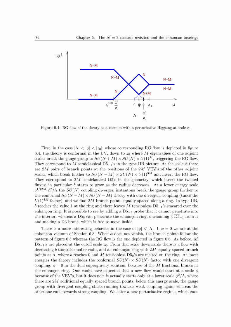
94 Chapter 6. The N = 2 cascade revisited and the enhancon bearings
1/g2i
N+M
N+M
N+M
NN−M
NN−M
N−M
µ0zφ
φΛ
Λ
1/2Mq φΛ
2
2
Figure 6.4: RG flow of the theory at a vacuum with a perturbative Higgsing at scale φ.
First, in the case |Λ| < |φ| < |z0|, whose corresponding RG flow is depicted in figure6.4, the theory is conformal in the UV, down to z0 where M eigenvalues of one adjointscalar break the gauge group to SU(N +M)× SU(N)×U(1)M , triggering the RG flow.They correspond to M semiclassical D5−1’s in the type IIB picture. At the scale φ thereare 2M pairs of branch points at the positions of the 2M VEV’s of the other adjointscalar, which break further to SU(N −M)× SU(N)× U(1)3M and invert the RG flow.They correspond to 2M semiclassical D5’s in the geometry, which invert the twistedfluxes; in particular b starts to grow as the radius decreases. At a lower energy scaleq1/(2M)φ2/Λ the SU(N) coupling diverges, instantons break the gauge group further tothe conformal SU(N −M)× SU(N −M) theory with one divergent coupling (times theU(1)4M factor), and we find 2M branch points equally spaced along a ring. In type IIB,b reaches the value 1 at the ring and there leaves M tensionless D5−1’s smeared over theenhancon ring. It is possible to see by adding a D5−1 probe that it cannot penetrate intothe interior, whereas a D50 can penetrate the enhancon ring, unchaining a D5−1 from itand making a D3 brane, which is free to move inside.
There is a more interesting behavior in the case of |φ| < |Λ|. If φ = 0 we are at theenhancon vacuum of Section 6.3. When φ does not vanish, the branch points follow thepattern of figure 6.5 whereas the RG flow is the one depicted in figure 6.6. As before, MD5−1’s are placed at the cutoff scale z0. From that scale downwards there is a flow withdecreasing b towards smaller radii, and an enhancon ring with 2M equally spaced branchpoints at Λ, where b reaches 0 and M tensionless D50’s are melted on the ring. At lowerenergies the theory includes the conformal SU(N) × SU(N) factor with one divergentcoupling: b = 0 in the dual supergravity solution, because of the M fractional branes atthe enhancon ring. One could have expected that a new flow would start at a scale φbecause of the VEV’s, but it does not: it actually starts only at a lower scale φ2/Λ, wherethere are 2M additional equally spaced branch points; below this energy scale, the gaugegroup with divergent coupling starts running towards weak coupling again, whereas theother one runs towards strong coupling. We enter a new perturbative regime, which ends

6.5. More supergravity duals: enhancon bearings 95
é
é
é
é
é
é
é
é
é
é
é
é
é
é
é
é
é
é
é
é
é
é
é
é
é
é
é
é
é
é
é
é
é
é
é
é
é
é
é
é
é
é
é
é
é
é
é
é
é
é
é
é
é
é
é
é
é
é
é
é
é
é
é
é
é
é
é
é
é
é
é
é
é
é
é
é
é
é
é
éé
é
é
é
é
é
é
é
é
ééé
é
é
é
é
é
é
é
é
é
é
é
é
é
é
é
é
ééé
é
é
é
é
é
é
é
é
éé
é
é
é
é
é
é
é
é
ééé
é
é
é
é
é
é
é
é
é
é
é
é
é
é
é
é
ééé
é
é
é
é
é
é
é
é
é
Figure 6.5: Branch points of the U(20)×U(20) theory at a vacuum with one enhancon bearing,a non-perturbative region between two enhancon rings. Red (blue) circles denote branch pointsrelated to the S (R) polynomial.
with a final ring of equally spaced branch points at scale q1/(2M) φ2/Λ where one gaugecoupling diverges; in the interior we find a new conformal SU(N −M) × SU(N −M)sector, with one divergent coupling, down to the IR.
We will call the ring at scale φ2/Λ an anti-enhancon. From the supergravity point ofview it is indistinguishable from a usual enhancon. However from the field theory point ofview it is quite peculiar: it represents instantonic effects that break the upper conformaltheory to a running one. These effects at the scale φ2/Λ are triggered by VEV’s at thescale φ: they take some “affine RG time” to break the group; moreover this means thatthe effective conformal theory must have some remnant of the scale Λ. These issuesdeserve further investigations.
We dub the regions between enhancon and anti-enhancon rings, where b ∈ Z and thetheory enjoys a superconformal phase, enhancon bearings.
It turns out that one can construct two different type IIB solutions that describe thisRG flow. The first one, say Higgsing-inspired (H), by continuity with the case |φ| > |Λ|where a perturbative Higgs mechanism takes place, interprets the ring of branch pointsat φ2/Λ as an anti-enhancon made of M tensionless D50’s (like the ones at Λ), whichtherefore force b to grow as the radius decreases, so that it remains bounded by 0 and1. The innermost ring, placed where b reaches 1, is an enhancon ring made of smearedtensionless D5−1. In this picture the D50’s (D5−1’s) are always associated to the first(second) gauge group.
The second, say cascade-inspired (C), works by analogy with the Klebanov-Tseytlin-Strassler N = 1 cascade and interprets the ring of branch points at φ2/Λ as an anti-enhancon made of M tensionless D50, and b becomes negative at smaller radii. Then b ismonotonic, and the innermost ring at b = −1 is interpreted as an enhancon ring made ofM tensionless D51. This is the picture that matches with the solution in (6.12)-(6.13) andwhich is usually considered in the literature. The association between fractional branesand gauge groups is such that wrapped (anti)D5 branes always correspond to the larger(smaller) gauge group.

96 Chapter 6. The N = 2 cascade revisited and the enhancon bearings
1/g
N+MN+M
N+M
N
i
2
µ
N
NN
N−M
N−M
N−M
0ΛφΛφ2
Λφ2
q 1/2M z
Figure 6.6: RG flow of the theory at a vacuum with one enhancon bearing. The theory iseffectively the conformal SU(N)× SU(N) between the scales Λ and φ2/Λ.
Type IIB solutions like the two we are discussing here can be explicitly constructedby excising and gluing twisted fields of the solution in (6.12)-(6.13) (possibly generatedby one or the other kind of fractional branes) and of a fluxless solution, with suitablesources accounting for the discontinuities at the glued surfaces, along the lines of [177].As already stressed in the case of the ordinary enhancon ring, this excision and gluingprocedure works for twisted fields, which are constrained to the orbifold fixed plane.Instead, untwisted fields like the metric can propagate also in the four dimensions of theorbifold, and must be computed once the twisted fields and fractional brane configurationis specified; this will be done in section 6.6. It should be remarked that they turn outto be the same in the two pictures. One immediately realizes that all gauge invariantquantities one could compute from the two solutions will give the same answer, and inthe field theory moduli space we have only one vacuum to match with the two solutions.This suggests that an ambiguity must be at work.
The ambiguity is particularly apparent in the T-dual type IIA/M-theory description.In type IIA, on each NS5-brane there is some worldvolume G1 = dA0 flux. Space-timefilling I3 brane intersections of codimension two, where D4 branes end on an NS5 brane,are magnetic sources for A0; the flux
∮G1 through any closed path in the 2 dimensions of
the NS5 worldvolume parametrized by v, in which I3 branes are points, jumps by one unitwhenever the path crosses one of these points. In what follows we will consider circularpaths centered in the origin of the v plane. One direction transverse to the NS5’s, say x6,is compact of radius R and the distance between the two NS5-branes is 2πbR. In figure6.7(a) we plotted the local geometry around a ring where the perturbative Higgsing takesplace as in the RG flow of figure 6.4: the NS5 on the left has a flux
∮G1 = −M (in
suitable units) below the stretched D4 branes, that jumps to M above the D4’s, whilethe opposite happens to the NS5 on the right whose flux jumps from M to −M . Alonga generalized enhancon ring b is integer valued, so that the stretched D4’s are degenerateand the NS5’s touch, as in figure 6.7(b). This interpretation leads to the H-picture inIIB: b has a saw-shaped profile bounded by [0, 1] and there are 2M fractional branes ofone kind in the enhancon bearing, M on each boundary. But the same IIA configuration

6.5. More supergravity duals: enhancon bearings 97
NS51
NS52
NS52
NS51
L(v) 0
NS51 NS52
−M
M
−M
M
H−picture
C−picture
M
−M
M
−M
−M
M−M
M
L(v)
|v|
x6
(b)(a)
D4 ’s
Figure 6.7: IIA description and ambiguity. (a) a point of the moduli space where 2M D4 branesare stretched between two NS5 branes. (b) another point where the D4 branes have collapsedto zero length. In the H-picture we interpret the D4 branes as still present, providing bendingtension and flux jump; in the C-picture, the D4 branes are simply not there.
can be equally well interpreted as two NS5 branes that just cross, without any D4 branesbetween them and without any jump in the flux. This leads to the C-picture in IIB: bis monotonic, and the bearing has fractional branes on one side and anti-fractional onthe other side, which cancel their charge. In the type IIA picture there is clearly a singleconfiguration (dual to a single vacuum in field theory) which gives rise to two pictures inIIB.
In type IIB, the ambiguity is related to S-duality: the duality group PSL(2,Z) actscovariantly on the parameter space, whilst the left over Z2 that acts as (B2, C2) →(−B2,−C2) and (b, c)→ (−b,−c) on the twisted fields, is gauged. The novel feature hereis that the enhancon bearings are domain walls on the C orbifold line, and the Z2 can acton each domain separately. At the same time, as already stressed, the ambiguity doesnot affect the untwisted fields: F5 and the warp factor are the same in the two pictures,since they depend on the twisted fields only quadratically in their field strengths; B2 andC2 are zero in the bulk.
We can keep playing the same game of adding suitable VEV’s, explained so far in thissection, to the newly found solutions, so as to generate longer and longer RG flows withmore and more transitions and reductions of degrees of freedom. Of course the number ofsteps is at most [N/M ]−. In this way we produce a class of vacua with a sort of cascadingbehavior, with cascades of different lengths.
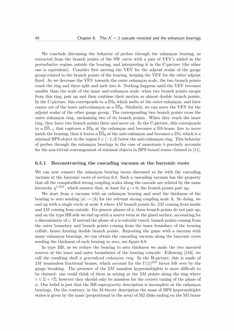
98 Chapter 6. The N = 2 cascade revisited and the enhancon bearings
We conclude discussing the behavior of probes through the enhancon bearing, asextracted from the branch points of the SW curve with a pair of VEV’s added in theperturbative regime outside the bearing, and interpreting it in the C-picture (the otherone is equivalent). Consider first moving the VEV for the adjoint scalar of the gaugegroup related to the branch points of the bearing, keeping the VEV for the other adjointfixed. As we decrease the VEV towards the outer enhancon scale, the two branch pointsreach the ring and there split and melt into it. Nothing happens until the VEV becomessmaller than the scale of the inner anti-enhancon scale, when two branch points escapefrom this ring, pair up and then continue their motion as almost double branch points.In the C-picture, this corresponds to a D50 which melts at the outer enhancon, and latercomes out of the inner anti-enhancon as a D50. Similarly, we can move the VEV for theadjoint scalar of the other gauge group. The corresponding two branch points cross theouter enhancon ring, unchaining two of its branch points. When they reach the innerring, they leave two branch points there and move on. In the C-picture, this correspondsto a D5−1 that captures a D50 at the enhancon and becomes a D3-brane, free to moveinside the bearing; then it leaves a D50 at the anti-enhancon and becomes a D51 which is aminimal BPS object in the region b ∈ [−1, 0] below the anti-enhancon ring. This behaviorof probes through the enhancon bearings in the case of monotonic b precisely accountsfor the non-trivial rearrangement of minimal objects in BPS bound states claimed in [11].
6.5.1 Reconstructing the cascading vacuum at the baryonic roots
We can now connect the enhancon bearing vacua discussed so far with the cascadingvacuum at the baryonic roots of section 6.4. Such a cascading vacuum has the propertythat all the complexified strong coupling scales along the cascade are related by the samehierarchy q1/2M , which ensures that, at least for q → 0, the branch points pair up.
We start from a vacuum with an enhancon bearing and send the thickness of thebearing to zero sending |φ| → |Λ| for the relevant strong coupling scale Λ. So doing, weend up with a single circle at scale Λ where 4M branch points lie, 2M coming from insideand 2M coming from outside. For generic phases of φ, these branch points do not pair up,and on the type IIB side we end up with a source term at the glued surface, accounting fora discontinuity of c. If instead the phase of φ is suitably tuned, branch points coming fromthe outer boundary and branch points coming from the inner boundary of the bearingcollide, hence forming double branch points. Repeating the game with a vacuum withmany enhancon bearings, we can obtain the cascading vacuum along the baryonic rootssending the thickness of each bearing to zero, see figure 6.8.
In type IIB, as we reduce the bearing to zero thickness we make the two smearedsources at the inner and outer boundaries of the bearing coincide. Following [134], wecall the resulting shell a generalized enhancon ring. In the H-picture, this is made of2M tensionless fractional branes, which account for the U(1)2M factor left over by thegauge breaking. The presence of the 2M massless hypermultiplets is more difficult tobe claimed: one could think of them as arising at the 2M points along the ring whereγ ∈ Z+ τZ; however they should only be massless for the correct tuning of the phase ofφ. Our belief is just that the IIB supergravity description is incomplete at the enhanconbearings. On the contrary, in the M-theory description the mass of BPS hypermultipletstates is given by the mass (proportional to the area) of M2 disks ending on the M5 brane
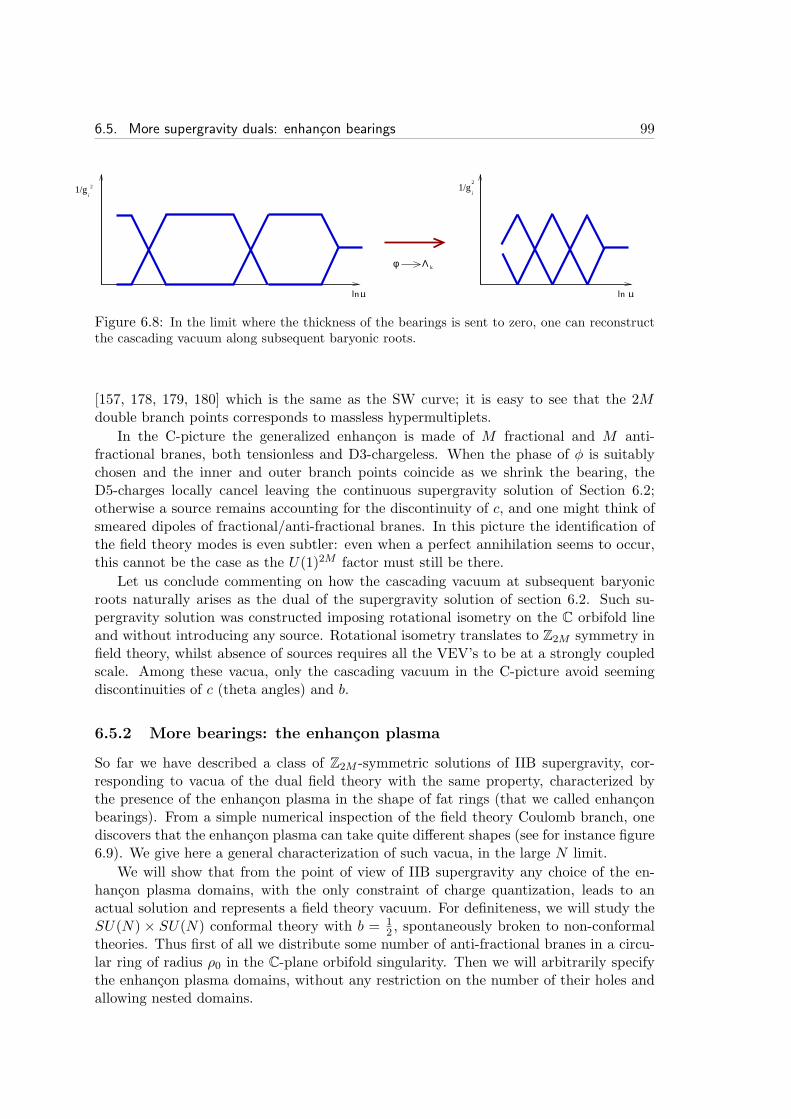
6.5. More supergravity duals: enhancon bearings 99
1/g
ln
1/g
µ
i
22
ln µ
kφ Λ
i
Figure 6.8: In the limit where the thickness of the bearings is sent to zero, one can reconstructthe cascading vacuum along subsequent baryonic roots.
[157, 178, 179, 180] which is the same as the SW curve; it is easy to see that the 2Mdouble branch points corresponds to massless hypermultiplets.
In the C-picture the generalized enhancon is made of M fractional and M anti-fractional branes, both tensionless and D3-chargeless. When the phase of φ is suitablychosen and the inner and outer branch points coincide as we shrink the bearing, theD5-charges locally cancel leaving the continuous supergravity solution of Section 6.2;otherwise a source remains accounting for the discontinuity of c, and one might think ofsmeared dipoles of fractional/anti-fractional branes. In this picture the identification ofthe field theory modes is even subtler: even when a perfect annihilation seems to occur,this cannot be the case as the U(1)2M factor must still be there.
Let us conclude commenting on how the cascading vacuum at subsequent baryonicroots naturally arises as the dual of the supergravity solution of section 6.2. Such su-pergravity solution was constructed imposing rotational isometry on the C orbifold lineand without introducing any source. Rotational isometry translates to Z2M symmetry infield theory, whilst absence of sources requires all the VEV’s to be at a strongly coupledscale. Among these vacua, only the cascading vacuum in the C-picture avoid seemingdiscontinuities of c (theta angles) and b.
6.5.2 More bearings: the enhancon plasma
So far we have described a class of Z2M -symmetric solutions of IIB supergravity, cor-responding to vacua of the dual field theory with the same property, characterized bythe presence of the enhancon plasma in the shape of fat rings (that we called enhanconbearings). From a simple numerical inspection of the field theory Coulomb branch, onediscovers that the enhancon plasma can take quite different shapes (see for instance figure6.9). We give here a general characterization of such vacua, in the large N limit.
We will show that from the point of view of IIB supergravity any choice of the en-hancon plasma domains, with the only constraint of charge quantization, leads to anactual solution and represents a field theory vacuum. For definiteness, we will study theSU(N) × SU(N) conformal theory with b = 1
2 , spontaneously broken to non-conformaltheories. Thus first of all we distribute some number of anti-fractional branes in a circu-lar ring of radius ρ0 in the C-plane orbifold singularity. Then we will arbitrarily specifythe enhancon plasma domains, without any restriction on the number of their holes andallowing nested domains.
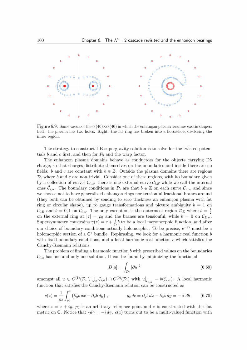
100 Chapter 6. The N = 2 cascade revisited and the enhancon bearings
é
é
é
é
é
é
é
é
é
é
é
é
é
é
é
é
éé
é
é
é
é
éé
é
é
é
é
é
é
é
é
é
é
é
é
é
é
é
éé
é
é
é
é
é
é
é
é
é
é
é
é
é
é
éé
é
é
é
é
é
é
éé
é
é
é
é
é
é
é
é
é
é
é
é
é
é
éé
é
é
é
é
é
é
éééééééééé
é
é
é
é
é
é
éééééééééé
é
é
é
é
é
é
éé
é
é
é
é
é
é
éééééééééé
é
é
é
é
é
é
éééééééééé
é
é
é
é
é
é
é
é
é
é
é
é
é
é
é
é
é
é
é
é
é
é
é
é
é
é
é
é
é
é
é
é
é
é
é
é
é
é
é
é
é
é
é
é
é
é
é
é
é
é
é
é
é
é
é
é
é
é
é
é
é
é
é
é
é
é
é
é
é
é
é
é
é
é
é
é
é
é
é
é
é
é
é
é
é
é
é
é
é
é
é
é
é
é
é
é
ééé
é
é
é
é
é
é
é
é
é
é
é
é
é
é
é
é
é
éé
é
é
é
é
é
é
é
é
éé
é
é
é
é
é
é
é
é
ééé
é
é
é
é
é
é
é
é
é
é
é
é
é
é
é
é
é
éé
é
é
é
é
é
é
é
é
é
Figure 6.9: Some vacua of the U(40)×U(40) in which the enhancon plasma assumes exotic shapes.Left: the plasma has two holes. Right: the fat ring has broken into a horseshoe, disclosing theinner region.
The strategy to construct IIB supergravity solution is to solve for the twisted poten-tials b and c first, and then for F5 and the warp factor.
The enhancon plasma domains behave as conductors for the objects carrying D5charge, so that charges distribute themselves on the boundaries and inside there are nofields: b and c are constant with b ∈ Z. Outside the plasma domains there are regionsDi where b and c are non-trivial. Consider one of these regions, with its boundary givenby a collection of curves Ci,α: there is one external curve Ci,E while we call the internalones Ci,α. The boundary conditions in Di are that b ∈ Z on each curve Ci,α, and sincewe choose not to have generalized enhancon rings nor tensionful fractional branes around(they both can be obtained by sending to zero thickness an enhancon plasma with fatring or circular shape), up to gauge transformations and picture ambiguity b = 1 onCi,E and b = 0, 1 on Ci,α. The only exception is the outermost region DE where b = 1
2on the external ring at |z| = ρ0 and the branes are tensionful, while b = 0 on CE,α.Supersymmetry constrains γ(z) = c+ i
gsb to be a local meromorphic function, and after
our choice of boundary conditions actually holomorphic. To be precise, e−iγ must be aholomorphic section of a C
∗ bundle. Rephrasing, we look for a harmonic real function bwith fixed boundary conditions, and a local harmonic real function c which satisfies theCauchy-Riemann relations.
The problem of finding a harmonic function b with prescribed values on the boundariesCi,α has one and only one solution. It can be found by minimizing the functional
D[u] =
∫
Di
|∂u|2 (6.69)
amongst all u ∈ C(1)(Di \⋃
α Ci,α) ∩ C(0)(Di) with u∣∣Ci,α
= b(Ci,α). A local harmonic
function that satisfies the Cauchy-Riemann relation can be constructed as
c(z) =1
gs
∫ z
p0
(∂yb dx− ∂xb dy
), gs dc = ∂yb dx− ∂xb dy = − ∗ db , (6.70)
where z = x + iy, p0 is an arbitrary reference point and ∗ is constructed with the flatmetric on C. Notice that ∗dγ = −i dγ. c(z) turns out to be a multi-valued function with
6.5. More supergravity duals: enhancon bearings 101
monodromies which give a representation of the homology group of Di. However, as longas the twisted field-strength dc is concerned, this is globally defined.
As we will explain in section 6.6, the warp factor is obtained by solving a Poissonequation (6.75) on the orbifold C
2/Z2 × C, with two kinds of D3-charge source terms,both localized along the orbifold line. One is proportional to |∂zγ|2 and comes fromthe twisted fluxes. The other one is localized on the tensionful fractional branes in theexternal ring and represents their D3-charge. In general the brane density per unit lengthω along the ring is not constant but rather given by
ω = −1
2Re ∂tγ , (6.71)
where the derivative is taken tangent to the boundary. This comes from the Bianchi
identity dF3 ∼ δ(4)D5. On the boundaries of the enhancon plasma domains there are
fractional branes too with density (6.71), but they are tensionless as b ∈ Z inside. Thusthe only contribution of the latter kind comes from the circular cutoff ring at |z| = ρ0.We do not go into further details here, as the computation of the warp factor is fullyexplained in section 6.6. What matters is that there is always one and only one solutionnormalizable at infinity. The 5-form flux is then given by: gsF5 = (1 + ∗)dvol3,1 ∧ dZ−1.
So far we showed that for any choice of the enhancon plasma domains, we can in prin-ciple solve the supergravity equations. The last constraint is the D5-charge quantization,which amounts to the monodromy of c(z) being quantized
∮
dc ∈ 2Z , (6.72)
or in other terms e−iπγ being a single-valued function. A basis of monodromies is given by∆c(Ci,α) on the internal boundaries Ci,α, and the integral is the total number of fractionalbranes on them. As the solution only depends on the choice of the enhancon plasmaboundaries (and the value of b on them), (6.72) descends to a constraint (in fact the onlyone) for them.
The total D3-charge of the system is then easily determined. The contribution fromthe fluxes in all the regions Di is
Qflux3 =1
2
∑
i
∫
Di
dc ∧ db = −1
2
∑
i
∑
α
∫
Ci,α
b dc = −1
2
∑
i,α
b(Ci,α)∆c(Ci,α) . (6.73)
The contribution from the anti-fractional branes on the external cutoff ring can be readfrom (6.71) to be: Qcutoff
3 = −14
∮
ρ0dc, because b = 1
2 there. Since the external ring isthe external boundary CE,E of the outermost region DE , this contribution can be addedto (6.73) by formally considering b(CE,E) = 1 instead of 1/2. Notice that (6.73) is gaugeand picture invariant. However, for our choice of gauge and picture the total charge is
Qtotal3 =∑
i,α
(1− b(Ci,α)
)∆c(Ci,α) ≡ N , (6.74)
where we used that Ci,E = −∑α Ci,α in homology, and b(Ci,E) = 1. This expressioncounts the number of fractional (as opposed to anti-fractional) branes. And in fact the
102 Chapter 6. The N = 2 cascade revisited and the enhancon bearings
solution we constructed is dual to a vacuum of the SU(N) × SU(N) theory. It is clearthat if we want to embed this vacuum in a larger theory, we can simply add regular D3branes.
Summarizing, we have shown that any choice of enhancon plasma domains, up to thecharge quantization constraint, gives rise to a solution of IIB supergravity with sources.Taking the limit of zero thickness, we can also include generalized enhancons and isolatedbunches of fractional branes; bunches of regular branes are easily included as well. Eachof these solutions is dual to a vacuum on the Coulomb branch of the SU(N) × SU(N)SCFT. Even though we cannot be more specific about the exact map (it should be workedout by computing operator VEV’s holographically), this huge class of solutions helps incovering the moduli space of the dual field theory.
6.6 Excisions, warp factors and the cure of repulson singu-
larities
In this section we take into account the excision of twisted fields inside the enhanconring and bearings and work out the correct warp factor for a quite general rotationallysymmetric configuration of fractional branes, which will be useful to describe the enhanconvacuum of section 6.3, the cut off cascading vacuum of section 6.2, the infinite cascadevacuum of section 6.4.3 and the vacua with rotationally symmetric bearings of section6.5.
We stress once again that consistency of the configuration of fractional branes, inagreement with the dual field theory picture encoded in the SW curve, implies an excisionof the naive twisted field solution at enhancon rings. Unlike the situation of [156], wherethere is an enhancon shell of codimension 1 in the non-compact part of the internalgeometry, here we face enhancon rings having codimension 1 only for the twisted fieldswhich are constrained to live on the orbifold plane, but not for the bulk fields whichpropagate also in the four additional dimensions of the orbifold. Consequently, the usualexcision of [156, 177] works for twisted fields but not for untwisted fields; in particular,the warp factor has to be computed once and for all, once the correct configuration offractional branes and twisted fields describing some gauge theory vacuum is specified.
The equation which determines the warp factor Z follows from the modified Bianchiidentity for F5 in the presence of sources at the locations of tensionful (anti-)fractionalbranes; it is a Poisson’s equation which reads [10]
∆6Z + (4π2α′)2g2s |∂zγ|2 δ(4)(~x) + 2(4π2α′)2gs∑
i
Q(xi)δ(6)(x− xi) = 0 , (6.75)
where ∆6 is the 6-dimensional Laplacian and x = (~y, ~x) a 6-dimensional vector, ~y ≡(Re z, Im z) = (x4, x5) being a vector on the orbifold fixed plane R2 and ~x = (x6, . . . , x9)being a vector in the covering space R
4 of the orbifold. In the previous formula, Q(xi)is the gauge invariant D3 brane charge of a regular or (anti-)fractional D3 brane placedat xi, which depends on the object and on the value of fields at its position (in the caseof fractional branes). The sum runs over all tensionful fractional D3 branes as well asregular D3 branes along with their images.
We will first consider M tensionless fractional branes melted in an enhancon ring ofradius ρe in the fixed plane parametrized by z, together with M ‘cutoff’ anti-fractional
6.6. Excisions, warp factors and the cure of repulson singularities 103
branes at the M roots of zM = −zM0 , which are used to Higgs the conformal UV theoryat the scale ρ0 = |z0|. Here and in the following, ρe is the scale at which the excisionshould be performed and its actual value depends, case by case, on the vacuum one isactually considering. We will also impose that the total gauge invariant D3 brane chargeof the configuration be N +M , adding regular D3 branes at the origin when needed, sothat the dual gauge theory is SU(N +M)× SU(N +M) in the UV. Using the freedomof shifting the axion b by an integer via a large gauge transformation, we will also setb(ρ) = 0 for ρ < ρe. Finally, we will be general and place the cutoff anti-fractional branesat a scale ρ0 such that b(ρ0) can acquire any positive value; the gauge invariant D3 branecharge supported by each of the anti-fractional branes is therefore
−nf − b(ρ0) = [b(ρ0)]+ − b(ρ0) . (6.76)
In other words, these anti-fractional branes are D5 branes wrapped on −C, with −[b(ρ0)]+units of worldvolume flux on it. Being in the large M limit, we can safely approximatethe cutoff anti-fractional branes with a ring.
The warp factor gets different contributions. First of all, if there are some regularD3 branes at the origin, they source the usual term according to (6.5). Secondly, the Mcutoff anti-fractional branes, because of their tension, contribute the following term inthe ring approximation
Zring,M (ρ, σ; ρ0) = 8πgsMα′2 ([b(ρ0)]+ − b(ρ0))σ2 + ρ2 + ρ20
[(σ2 + ρ2 + ρ20)
2 − 4ρ20ρ2]3/2
, (6.77)
where ρ = |~y| and σ = |~x|. Fractional branes at the enhancon ring, being tensionless, donot contribute directly to the warp factor. Finally, there is a term sourced by the twistedfield strengths
dγ =iM
π
dz
zΘ(|z| − |ze|)Θ(|z0| − |z|) . (6.78)
In general it takes the form
Zfl(~y, ~x) = 4πα′2g2s
∫
d2z |∂zγ|21
[|~x|2 + |~y − ~z|2]2, (6.79)
which in the case under consideration reduces to
Zfl,M (ρ, r; ρe, ρ0) =2(gsMα′)2
r4
2 logr4 +
(
ρ2e +√
(r2 + ρ2e)2 − 4ρ2eρ
2)
r2 − 2ρ2eρ2
r4 +(
ρ20 +√
(r2 + ρ20)2 − 4ρ20ρ
2)
r2 − 2ρ20ρ2+
+ 2 logρ20ρ2e
+r2
r2 − ρ2
[
3(r2 − ρ2) + ρ20 − ρ2√
(r2 + ρ20)2 − 4ρ20ρ
2− 3(r2 − ρ2) + ρ2e − ρ2√
(r2 + ρ2e)2 − 4ρ2eρ
2
]
,
(6.80)
where r2 = ρ2 + σ2.Notice that the total D3 brane charge, which is N +M if the UV theory has gauge
group SU(N+M)×SU(N+M), gets sectioned in different pieces. The flux term carries acharge M b(ρ0), since b(ρ0) =
gsMπ log ρ0
ρe; the cutoff anti-fractional branes carry a charge
104 Chapter 6. The N = 2 cascade revisited and the enhancon bearings
M ([b(ρ0)]+ − b(ρ0)); finally, there are N − [b(ρ0)]−M regular D3 branes at the origin.This can be checked via the large r asymptotics of the different terms in the warp factor.
The vacuum considered in [152] and described in section 6.3 has N regular D3 branes
at the origin, the enhancon ring at ρ1 = e− π
2gsM ρ0, and M cutoff anti-fractional branesat ρ0, where b(ρ0) = 1
2 , carrying M/2 units of D3 charge; the twisted fluxes betweenfractional and anti-fractional branes carry other M/2 units of D3 charge.
The vacuum with a finite cascade starting at z0 and reaching SU(M) in the infraredhas no regular D3 branes at the origin, M fractional branes with no D3 charge melted at
an enhancon ring at ρmin = ρN/M ≡ e− πNgsM2 ρ1, andM cutoff anti-fractional branes at ρ0,
where b(ρ0) =NM + 1
2 , carrying againM/2 units of D3 charge; this time the twisted fluxesbetween fractional and anti-fractional branes carry N +M/2 units of D3 charge. As weexplained in detail in section 6.5, what happens is that at each generalized enhancon ringscale along the cascade (where b ∈ Z) melted tensionless fractional and anti-fractionalbranes are left, naively annihilating if c is continuous crossing radially the generalized
enhancon ring. In case N = lM + p is not a multiple of M , then ρmin = e− πlgsM ρ1,
b(ρ0) = l+ 12 and there are p D3 branes at the origin: the IR theory below the enhancon
scale is the SU(p)× SU(p) theory with one infinite coupling.
The infinite cascade limit can even be defined continuously: it is enough to sendcontinuously the cutoff ρ0 →∞ keeping ρmin fixed and b(ρmin) = 0. This can be achievedif b(ρ0) =
gsMπ ln ρ0
ρmin: as we change the cutoff ρ0, we also change the value of the gauge
couplings at the cutoff (and on the string side the tension of the cutoff branes) so that lowenergy physics is not modified. Notice that every time a b(ρ0) ∈ Z threshold is crossed,the total D3 brane charge of the configuration (the ranks of the UV CFT) jumps byM units, and the cutoff anti-fractional branes change. The warp factor for the infinitecascade with no regular D3 branes is nothing but Zfl,M (ρ, r; ρmin,∞), see eq. (6.80). Ifneeded, the addition of p regular D3 branes is straightforward.
We can also find the warp factor for a configuration with any number of rotationallysymmetric bearings. The total warp factor is sourced by twisted fluxes and possibly bycutoff anti-fractional branes, if there is no infinite cascade in the UV. Inside bearings fluxesvanish, whereas outside they take the usual form |dγ| = M
πdρρ . Therefore fluxes contribute
to the warp factor by a sum of terms taking the schematic form Zfl,M (ρ, r; ρ(i+1)> , ρ
(i)< ),
where ρ(i+1)> is the outer radius of the (i + 1)-th bearing and ρi< is the inner radius of
the i-th bearing, if the ordering points inwards. The requirement that ρ(i)< and ρ
(i+1)> be
boundaries of subsequent bearings translates into ρ(i)< = e
πnigsM ρ
(i+1)> , for some ni ∈ N.
Finally, by now it should also be clear how to write the warp factor in the case ofperturbative Higgsings by backreacting rings of tensionful fractional and anti-fractionalbranes, adding terms like (6.77) sourced at suitable radii and with the suitable normal-izations.
We end this section with some important remarks about the backreacted geometries.For concreteness, we concentrate on solutions without bearings nor perturbative Higgsingexcept at the cutoff, since the generalization of the statements we are about to makeshould be clear.
The warp factor diverges (and the gravitational potential felt by a massive particlehas an absolute minimum) only at the locations of sources for it (fractional branes and
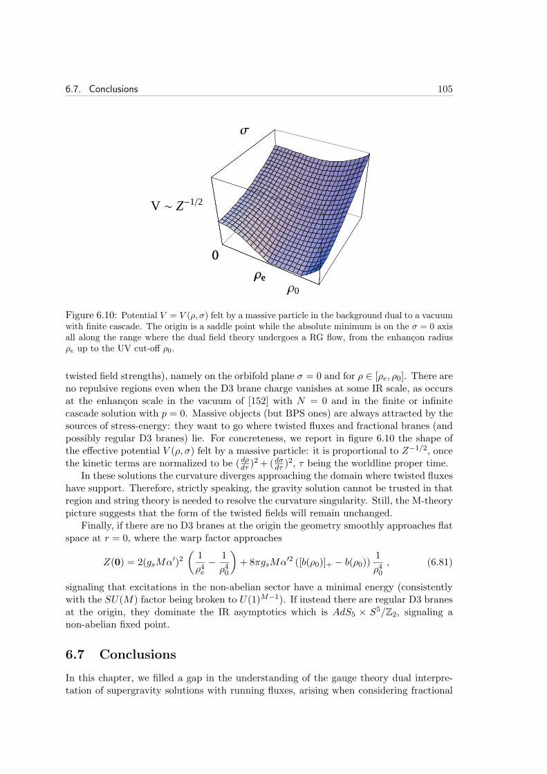
6.7. Conclusions 105
0
ΡeΡ0
Σ
V ~ Z-12
0
ΡeΡ
Σ
Figure 6.10: Potential V = V (ρ, σ) felt by a massive particle in the background dual to a vacuumwith finite cascade. The origin is a saddle point while the absolute minimum is on the σ = 0 axisall along the range where the dual field theory undergoes a RG flow, from the enhancon radiusρe up to the UV cut-off ρ0.
twisted field strengths), namely on the orbifold plane σ = 0 and for ρ ∈ [ρe, ρ0]. There areno repulsive regions even when the D3 brane charge vanishes at some IR scale, as occursat the enhancon scale in the vacuum of [152] with N = 0 and in the finite or infinitecascade solution with p = 0. Massive objects (but BPS ones) are always attracted by thesources of stress-energy: they want to go where twisted fluxes and fractional branes (andpossibly regular D3 branes) lie. For concreteness, we report in figure 6.10 the shape ofthe effective potential V (ρ, σ) felt by a massive particle: it is proportional to Z−1/2, oncethe kinetic terms are normalized to be ( dρdτ )
2 + (dσdτ )2, τ being the worldline proper time.
In these solutions the curvature diverges approaching the domain where twisted fluxeshave support. Therefore, strictly speaking, the gravity solution cannot be trusted in thatregion and string theory is needed to resolve the curvature singularity. Still, the M-theorypicture suggests that the form of the twisted fields will remain unchanged.
Finally, if there are no D3 branes at the origin the geometry smoothly approaches flatspace at r = 0, where the warp factor approaches
Z(0) = 2(gsMα′)2(
1
ρ4e− 1
ρ40
)
+ 8πgsMα′2 ([b(ρ0)]+ − b(ρ0))1
ρ40, (6.81)
signaling that excitations in the non-abelian sector have a minimal energy (consistentlywith the SU(M) factor being broken to U(1)M−1). If instead there are regular D3 branesat the origin, they dominate the IR asymptotics which is AdS5 × S5/Z2, signaling anon-abelian fixed point.
6.7 Conclusions
In this chapter, we filled a gap in the understanding of the gauge theory dual interpre-tation of supergravity solutions with running fluxes, arising when considering fractional
106 Chapter 6. The N = 2 cascade revisited and the enhancon bearings
branes at generic Calabi-Yau singularities. It has been known for some time that frac-tional branes at isolated singularities describe RG flows which can be described in termsof cascades of Seiberg dualities. A similar interpretation was not possible for branes atnon-isolated singularities, since their effective dynamics is intrinsically N = 2.
The basic outcome of our analysis is that, for branes at non-isolated singularities, thereduction of the gauge group ranks along the RG flow can be understood in terms of asequence of strong coupling transitions reminiscent of the low energy description of thebaryonic root of N = 2 SQCD. The energy range spanned by the cascade depends on thepoint in the Coulomb branch one is sitting at; specifically, on the number of non-vanishingVEV’s for the adjoint scalars.
We were also able to provide a gravity dual description of a new set of infinitelymany vacua, characterized by new geometric structures, the enhancon bearings, wherethe dual gauge theory alternates energy ranges where it runs, with ranges in which it isin a strongly coupled superconformal phase.
For all these vacua, an enhancon mechanism takes place in the far IR. This changesthe twisted fields configuration and ultimately the metric, whose correct repulson-freeexpression we provided for all vacua we have been studying.
We should also note that Stefano Cremonesi analysed further the IR of this model in[181], finding the exact twisted flux configuration corresponding to any Coulomb branchvacua (any Seiberg-Witten curve). The upshot of the analysis of [181] is that one shouldreally think of the N = 2 fractional branes as being transmuted into twisted flux. Inthat respect we see that the mechanism of resolution of the IR singularity at finite gs issimilar to the geometric transition for deformation fractional branes.
Our analysis focused, for definiteness, on the A1 singularity, but our results have amuch wider validity. First, they trivially extend to any N = 2 singularity, as for instancethe full ADE series. Second, any Calabi-Yau cone with non-isolated singularities, whichupon the inclusion of branes generically gives rise to a N = 1 theory, should presentthe same behavior. This is suggested from the supergravity solution and it is a rathernon-trivial claim since SW techniques are not available in the N = 1 context.
More complicated flows occur when fractional branes at isolated and non-isolatedsingularities are both present, which is in fact the most generic situation. In a genericcascade some cascade “steps” can be understood in terms of Seiberg duality, some ofthem cannot as the theory, due to the presence of adjoint fields, exhibits at some energiesan effective N = 2 behavior. We conjecture that in those cases too the rank reductionis due to the adjoint fields being at baryonic-root-like points of its moduli space. In thenext chapter we will consider several examples of such cascades of mixed type, findingperfect agreement with our proposal.

Chapter 7
Cascades of mixed kind andinterplay of various fractionalbranes
In this Chapter we find the KT-like solution for arbitrary fractional branes on a non-chiral quiver corresponding to a Z2 orbifold of the conifold. The geometry has non-isolatedsingularities, so we can consider simultaneously the various kinds of fractional branes, tostudy their interplay. This geometry was studied in the earlier work [182] with the hopethat one could brane-engineer dynamical SUSY breaking while bypassing the typicalrunaway instability (actually there is still a runaway direction along a baryonic branch,but the hope was to realize metastable DSB).
Our main reason to study this geometry here is because it is an interesting modelto apply the ideas of the previous Chapter about the N = 2 cascade in a more genericN = 1 context. This Chapter is based on [1], written with Riccardo Argurio, FrancescoBenini, Matteo Bertolini and Stefano Cremonesi. 1
7.1 Introduction
The correspondence between gauge theories with non-trivial low-energy dynamics andstring theory backgrounds has an enormous potential. The string theory setup is usuallyestablished drawing uniquely on the holomorphic data of a supersymmetric gauge theory,including a specific choice of vacuum. Then, solving the classical equations of motionof supergravity one can in principle obtain, through the warp factor, all the dynamicalinformations on the gauge theory low-energy dynamics, that would instead usually implyprecise knowledge of the Kahler sector. The limitation of this procedure to supergravityand not to full string theory corresponds in the gauge theory to taking some large N andstrong ’t Hooft coupling limit.
A fruitful arena where to address these issues has proven to be that of D3-branes atCalabi-Yau (CY) singularities. In this context, the most celebrated example where such
1Actually the paper [1] was written before [2], and it gave the motivation to further study N = 2cascades, when we realized that they were poorly understood.
107
108 Chapter 7. Cascades of mixed kind and interplay of various fractional branes
a program has been successfully completed is the warped deformed conifold [118], whichdescribes a theory with confinement and chiral symmetry breaking.
It is of obvious interest to apply the above program to gauge theories with a variedlow-energy behavior. D3-branes at CY singularities typically give rise to N = 1 quivergauge theories, which are supersymmetric theories characterized by product gauge groups,matter in the bifundamental representation and a tree level superpotential, all such databeing dictated by the structure of the singularity. Most quiver gauge theories can haveseveral different IR behaviors, depending on which branch of the moduli space one issitting on. Already in the simple conifold theory, one has a baryonic branch displayingconfinement and a mass gap in the gauge sector, and mesonic branches with a dynamicswhich is N = 4 to a good approximation. In more general quivers, other kinds of low-energy behaviors are possible. Some quivers will actually have no vacua and display arunaway behavior [149, 148, 150, 151], but this leaves little hope of finding a regulargravity dual. Other quivers will on the other hand contain branches of the moduli spacewhere the dynamics is approximately the one on the Coulomb branch of an N = 2 theory.The latter can also be thought of as mesonic branches, albeit of complex dimension oneinstead of three as in the (generic) N = 4 case.
In this chapter, we construct the gravity dual of the most generic gauge theory onecan engineer using D3-branes at the tip of a Zk non-chiral orbifold of the conifold [56],focusing for simplicity, but with little loss of generality, on the case k = 2. This singularityadmits different kinds of fractional branes, triggering confinement or enjoying an N = 2mesonic branch and known as deformation or N = 2 fractional branes, respectively.We aim at describing the backreaction of the most general D3-brane bound state. Thedifficulty in doing so stems from the fact that the UV completion which corresponds to thesupergravity solution is qualitatively different in the two cases. For deformation branes,the renormalization group (RG) flow is best described in terms of a cascade of Seibergdualities which increases the overall rank of the quiver nodes towards the UV. For N = 2branes, the RG flow (which is indeed present and also increases the ranks towards theUV [10, 11]) seems to be better represented by some form of non-perturbative Higgsing,as argued in the previous chapter.
It should be clear that whenever there are N = 2 branes around the IR of the gravitydual is bound to contain some singularity. This is because open string degrees of freedomcannot completely transmute into flux. Indeed, on the Coulomb branch we still have bydefinition some surviving abelian gauge group, which cannot be described in terms ofclosed string degrees of freedom. This situation is similar to the situation where one aimsat describing theories with flavors. There too, flavor degrees of freedom must be describedby open strings, and hence flavor branes must be present in the gravity dual as physicalsources [183]. Thus in our set up we expect to have physical sources corresponding toN = 2 fractional branes. The main difference with respect to the case of flavor branes isthat N = 2 fractional branes are not infinitely extended in the Calabi-Yau.
The main results of our analysis can be summarized as follows. We find an explicitsupergravity solution describing a generic distribution of fractional branes, both of thedeformation and N = 2 kind, on the orbifolded conifold, and corresponding to the UVregime of the dual gauge theory. It describes holographically an RG flow which exactlymatches the beta functions that one can compute in the dual field theory and the expectedreduction of degrees of freedom towards the IR, which occurs through a cascade. We

7.2. The orbifolded conifold 109
Figure 7.1: The quiver diagram of the gauge theory, for the most generic choice of ranks.Circles represent unitary gauge groups, arrows represent bifundamental chiral superfields. Forlater purposes we have parametrized the four independent ranks in terms of a common N .
develop an algorithm to follow the RG flow of each gauge coupling from the supergravitysolution. An interesting feature is that in this general setting there are cascade stepsthat do not always have a simple interpretation in terms of Seiberg dualities. This isdue to the presence of N = 2 fractional branes, or more generally to the presence oftwisted fluxes. Nevertheless, supergravity considerations and field theory expectations(based on the non-holomorphic beta function) exactly match. As far as the IR regime isconcerned, we perform a non-trivial consistency check matching the field theory effectivesuperpotential with that predicted from the geometric background. We also provide thesolution for the 3-form fluxes and discuss the pattern of singularities resolution, while weonly set the stage for computing the exact warp factor in this case.
This chapter is structured as follows. In section 7.2 we explain our set up and introducethe minimal geometrical data that is needed in the following. In section 7.3 we presentthe supergravity solution which is expected to reproduce the UV behavior of our quivergauge theory. We take the CY base to be the orbifold of the singular conifold, butwe take into account all the fluxes sourced by the fractional branes and compute theirbackreaction on the warp factor. We then check that the result is indeed compatiblewith the expected RG flow and perform a number of non-trivial gauge/gravity dualitychecks. In section 7.4 we discuss the extension of the previous solution towards theIR, discuss the singularity structure of our solution, their resolutions, and match theeffective superpotential obtained on the two sides of the correspondence. The appendicescontain many technical data which might help in better understanding the form of thesupergravity ansatz that we solve in the main text and the geometric structure of theorbifolded conifold CY singularity we consider.
7.2 The orbifolded conifold
We consider in what follows an orbifolded avatar of the familiar conifold quiver. Wefocus on a non-chiral Z2 orbifold of the conifold and consider the corresponding N = 1supersymmetric quiver gauge theory obtained by placing a bound state of regular andfractional D3-branes at its tip. This theory has been analyzed at great length in [182],to which we refer for more details.
The quiver gauge theory is shown in Figure 7.1. The gauge theory has four gauge
110 Chapter 7. Cascades of mixed kind and interplay of various fractional branes
factors and a tree level superpotential for the bifundamental fields
W = λ (X12X21X14X41 −X23X32X21X12 +X34X43X32X23 −X41X14X43X34) , (7.1)
where Xij is a chiral superfield in the fundamental representation of the i-th gauge groupand antifundamental representation of the j-th gauge group, and traces on the gaugedegrees of freedom are understood.
We are interested in the dynamics of the gauge theory with the most generic rankassignment, as in Figure 7.1. Depending on the values of the Mi’s, various kinds ofIR dynamics can occur: confinement, runaway behavior or a (locally N = 2) quantummoduli space.
There is a relation between the ranks of the various gauge groups in the quiver andthe number of fractional branes wrapping the different 2-cycles in the geometry. In turn,the fractional branes source the RR 3-form flux which is an important ingredient in orderto determine the supergravity solution. In the following of this section we provide thelink between these three sets of data (ranks, branes wrapping cycles, fluxes). For a moredetailed discussion we refer to appendix F.2.
7.2.1 Regular and fractional branes
The superconformal theory (N 6= 0 , Mi = 0) can be engineered by placing N regularD3-branes at the tip of the cone. Unbalanced ranks in the quiver of Figure 7.1 corre-spond instead to the presence of fractional D3-branes and the corresponding breaking ofconformal invariance. From the gauge theory viewpoint, fractional branes correspond toindependent anomaly free rank assignments in the quiver (modulo the superconformalone). Hence, in the present case, we have three types of fractional branes to play with.
As reviewed in Section 5.4, fractional branes can be classified in terms of the IRdynamics they trigger [148].
The deformation fractional branes are those associated to a single node in the quiver,or to several decoupled nodes, or else to several contiguous nodes whose correspondingclosed loop operator appears in the tree level superpotential. This subsector of the quivergauge theory undergoes confinement. Examples of this kind in our theory correspond torank assignments (1, 0, 0, 0), (1, 0, 1, 0) or (1, 1, 1, 0) and cyclic permutations.
The N = 2 fractional branes are those associated to contiguous nodes in the quiverwhose corresponding meson does not appear as an individual term in the superpotential.Rank assignments corresponding to this class of branes in our quiver are for instance(1, 1, 0, 0) and cyclic permutations.
Finally, fractional branes of any other class (which is the most generic case, in fact)are DSB branes. They lead to ADS-like superpotential and runaway behavior. Geomet-rically, they are associated with geometries where the complex structure deformation isobstructed, this tension being the geometric counterpart of the runaway. In this case theoccupied nodes have unbalanced ranks.
Obviously, combining different fractional branes of a given class, one can obtain frac-tional branes of another class. Hence one can choose different fractional brane bases todescribe the gauge theory. In our present case, we will be able to choose a basis com-posed only of deformation and N = 2 fractional branes. We have just seen to which rank
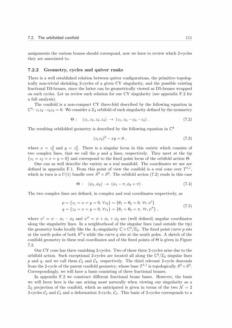
7.2. The orbifolded conifold 111
assignments the various branes should correspond, now we have to review which 2-cyclesthey are associated to.
7.2.2 Geometry, cycles and quiver ranks
There is a well established relation between quiver configurations, the primitive topolog-ically non-trivial shrinking 2-cycles of a given CY singularity, and the possible existingfractional D3-branes, since the latter can be geometrically viewed as D5-branes wrappedon such cycles. Let us review such relation for our CY singularity (see appendix F.2 fora full analysis).
The conifold is a non-compact CY three-fold described by the following equation inC4: z1z2−z3z4 = 0. We consider a Z2 orbifold of such singularity defined by the symmetry
Θ : (z1, z2, z3, z4) → (z1, z2,−z3,−z4) . (7.2)
The resulting orbifolded geometry is described by the following equation in C4
(z1z2)2 − xy = 0 , (7.3)
where x = z23 and y = z24 . There is a singular locus in this variety which consists oftwo complex lines, that we call the p and q lines, respectively. They meet at the tipz1 = z2 = x = y = 0 and correspond to the fixed point locus of the orbifold action Θ.
One can as well describe the variety as a real manifold. The coordinates we use aredefined in appendix F.1. From this point of view the conifold is a real cone over T 1,1,which in turn is a U(1) bundle over S2 × S2. The orbifold action (7.2) reads in this case
Θ : (φ1, φ2) → (φ1 − π, φ2 + π) . (7.4)
The two complex lines are defined, in complex and real coordinates respectively, as
p = z1 = x = y = 0, ∀z2 = θ1 = θ2 = 0, ∀r, ψ′q = z2 = x = y = 0, ∀z1 = θ1 = θ2 = π, ∀r, ψ′′ , (7.5)
where ψ′ = ψ − φ1 − φ2 and ψ′′ = ψ + φ1 + φ2 are (well defined) angular coordinatesalong the singularity lines. In a neighborhood of the singular lines (and outside the tip)the geometry looks locally like the A1-singularity C×C
2/Z2. The fixed point curve p sitsat the north poles of both S2’s while the curve q sits at the south poles. A sketch of theconifold geometry in these real coordinates and of the fixed points of Θ is given in Figure7.2.
Our CY cone has three vanishing 2-cycles. Two of these three 2-cycles arise due to theorbifold action. Such exceptional 2-cycles are located all along the C
2/Z2 singular linesp and q, and we call them C2 and C4, respectively. The third relevant 2-cycle descendsfrom the 2-cycle of the parent conifold geometry, whose base T 1,1 is topologically S2×S3.Correspondingly, we will have a basis consisting of three fractional branes.
In appendix F.2 we construct different fractional brane bases. However, the basiswe will favor here is the one arising most naturally when viewing our singularity as aZ2 projection of the conifold, which as anticipated is given in terms of the two N = 22-cycles C2 and C4 and a deformation 2-cycle, Cβ . This basis of 2-cycles corresponds to a
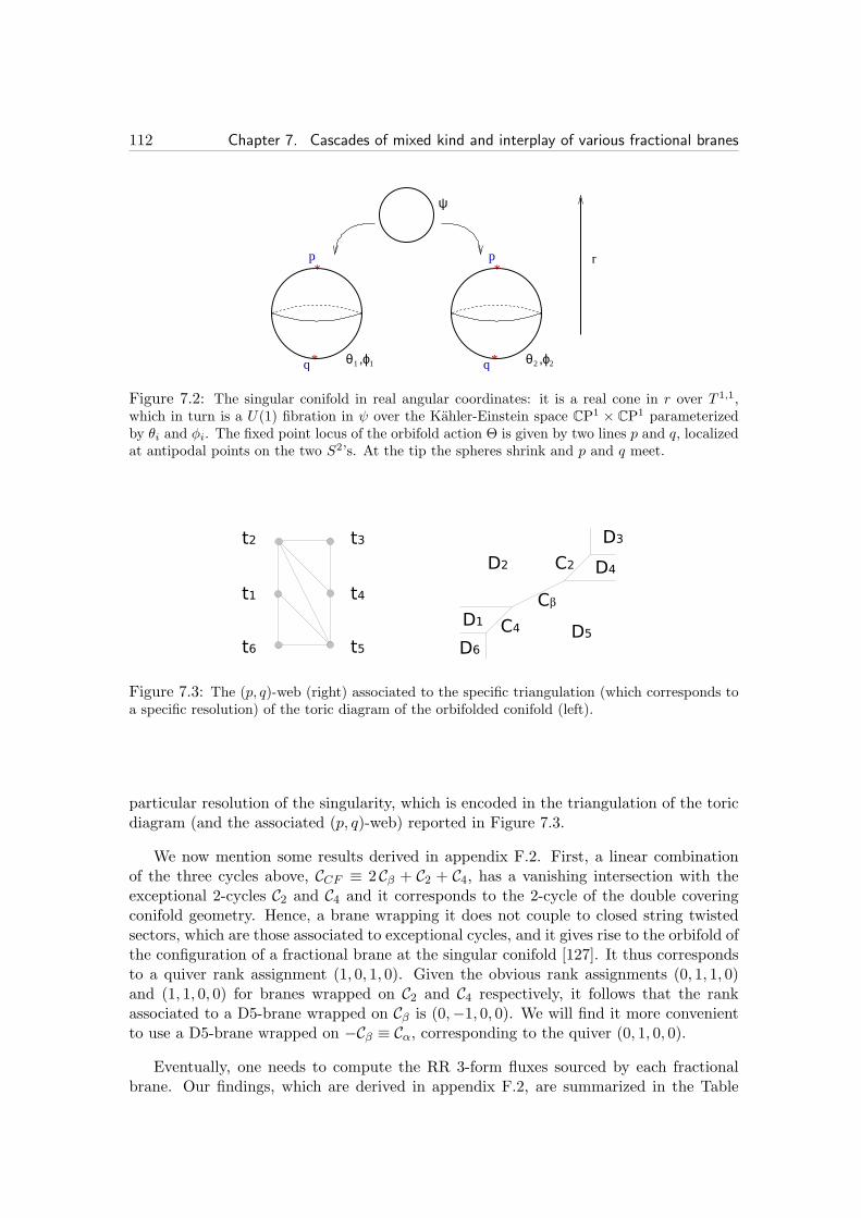
112 Chapter 7. Cascades of mixed kind and interplay of various fractional branes
1 1θ ,ϕ
*
*
p*
*
p
2 2θ ,ϕ
ψ
r
q q
Figure 7.2: The singular conifold in real angular coordinates: it is a real cone in r over T 1,1,which in turn is a U(1) fibration in ψ over the Kahler-Einstein space CP1 × CP1 parameterizedby θi and φi. The fixed point locus of the orbifold action Θ is given by two lines p and q, localizedat antipodal points on the two S2’s. At the tip the spheres shrink and p and q meet.
Figure 7.3: The (p, q)-web (right) associated to the specific triangulation (which corresponds toa specific resolution) of the toric diagram of the orbifolded conifold (left).
particular resolution of the singularity, which is encoded in the triangulation of the toricdiagram (and the associated (p, q)-web) reported in Figure 7.3.
We now mention some results derived in appendix F.2. First, a linear combinationof the three cycles above, CCF ≡ 2 Cβ + C2 + C4, has a vanishing intersection with theexceptional 2-cycles C2 and C4 and it corresponds to the 2-cycle of the double coveringconifold geometry. Hence, a brane wrapping it does not couple to closed string twistedsectors, which are those associated to exceptional cycles, and it gives rise to the orbifold ofthe configuration of a fractional brane at the singular conifold [127]. It thus correspondsto a quiver rank assignment (1, 0, 1, 0). Given the obvious rank assignments (0, 1, 1, 0)and (1, 1, 0, 0) for branes wrapped on C2 and C4 respectively, it follows that the rankassociated to a D5-brane wrapped on Cβ is (0,−1, 0, 0). We will find it more convenientto use a D5-brane wrapped on −Cβ ≡ Cα, corresponding to the quiver (0, 1, 0, 0).
Eventually, one needs to compute the RR 3-form fluxes sourced by each fractionalbrane. Our findings, which are derived in appendix F.2, are summarized in the Table

7.3. Supergravity background for the UV regime 113
below:−∫
A2F3 −
∫
A4F3 −
∫
ACFF3 gauge theory
D5 on C2 2 0 0 (0, 1, 1, 0)D5 on C4 0 2 0 (1, 1, 0, 0)D5 on Cα 1 1 −1 (0, 1, 0, 0)
(7.6)
where fluxes are understood in units of 4π2α′gs. The 3-cycle A2 corresponds to theproduct of the exceptional 2-cycle C2 transverse to the p-line with the S1 on p. Similarly,A4 is the product of the exceptional C4 with the S1 in the q-line. Finally, ACF is the imageof the compact 3-cycle of the double covering conifold under the orbifold projection.
The table above is all we need to translate directly a quiver with generic rank assign-ment to a supergravity solution with the corresponding 3-form flux.
7.3 Supergravity background for the UV regime
In this section we present the supergravity solution describing the most general D3-brane system one can consider on the orbifolded conifold. The solution is expected tobe dual to the previously discussed gauge theory with the most general rank assignment:(N +M1, N +M2, N +M3, N).2
Fractional branes are magnetic sources for the RR 3-form flux. This typically resultsin some singularity of the backreacted supergravity solution. In some cases, namely whenthere are only deformation branes around, the singularity is smoothed out by the complexstructure deformation the branes induce. One gets back a singularity-free solution wherebranes are replaced by fluxes [118, 140]. In more general situations it is more difficult tofind a regular solution. As already noticed, in the case of N = 2 fractional branes this isin fact not even expected to be possible, because there should always be some remainingopen string modes corresponding to the left over U(1)N−1 gauge degrees of freedom onthe Coulomb branch. Hence, (a remnant of) the brane sources remains in the gravitydual.
This said, in order to take the leading effect of any such kind of fractional brane intoaccount, it is enough to make an educated ansatz for the supergravity fields and to imposesuitable boundary conditions on the system of differential equations. Therefore, in whatfollows, we will only consider the type IIB bulk action SIIB, eq. (A.1), and implementthe effects of each brane source by properly chosen boundary conditions.
7.3.1 The UV regime: running fluxes and singularity lines
The general solution we are looking for has constant axio-dilaton τ = C0 + ie−Φ = i, butnon-trivial RR and NSNS 3-form fluxes (which are usually organized in a complex 3-formG3 = F3+ ie
−ΦH3 = F3+ iH3), RR 5-form field strength F5 and warp factor. The ansatzreads
ds210 = h−1/2dx23,1 + h1/2(dr2 + r2ds2T 1,1)
F5 = (1 + ∗10) dh−1 ∧ dvol3,1G3 = GU3 +GT3
(7.7)
2Our conventions for type IIB supergravity and D-brane actions, together with the equations of motionfor the bulk fields, can be found in appendix A.
114 Chapter 7. Cascades of mixed kind and interplay of various fractional branes
where the orbifold Z2 identification (7.2) acting on the internal coordinates is understood,h is the warp factor, while the superscripts U and T on the 3-form flux stand for untwistedand twisted sector fluxes, respectively. The above ansatz is the one of a warped singularcone. Any deformation of the singular geometry will still asymptote to this cone for largevalues of the radial coordinate, and it is in this sense that we will think of the solutionas representing (at least) the UV regime of the dual gauge theory.
Recall that for the solution to be supersymmetric, the complex 3-form G3 should be(2, 1), primitive and imaginary-self-dual [123]
∗6G3 = iG3 , (7.8)
where ∗6 is constructed with the unwarped metric. We will see that the warp factordepends on the radial coordinate as well as some of the angular coordinates, as typicalfor solutions with N = 2 branes around [10].
The equations of motion we have to solve are written in appendix A, eqs. (A.5).The warp factor equation is given by the BI for F5. The Einstein equations are thenautomatically satisfied by our ansatz (7.7).
It is easy to check that, given all the geometrical data discussed in the previous section,and taking for simplicity all fractional branes sitting at the tip, the complex 3-form G3
reads3
G3 = −α′
2gs (M1 −M2 +M3)
[
ωCF3 − 3idr
r∧ ωCF2
]
+ 2iπα′gs (−M1 +M2 +M3)dz2z2∧ ω(p)
2 + 2iπα′gs (M1 +M2 −M3)dz1z1∧ ω(q)
2
= −α′
2gs (M1 −M2 +M3)
[
ωCF3 − 3idr
r∧ ωCF2
]
+ iπα′gs (−M1 +M2 +M3)
(
3dr
r+ i dψ′
)
∧ ω(p)2
+ iπα′gs (M1 +M2 −M3)
(
3dr
r+ i dψ′′
)
∧ ω(q)2 ,
(7.9)
where ωCF3 and ωCF2 are defined in appendix F.1, and ω(p)2 and ω
(q)2 are the two normalized
exceptional 2-cocycles defined by the integrals below.
For the present purposes it suffices to recall that
∫
CCF
ωCF2 = 4π ,
∫
C2
ω(p)2 =
∫
C4
ω(q)2 = 1 , and
∫
ACF
ωCF3 = 8π2 , (7.10)
where ACF is the image under the orbifold projection of the 3-sphere on the doublecovering conifold. The second equality in (7.9) can be easily obtained by using eqs. (F.2-
3The vielbein we use for the singular conifold can be found in (F.9). Appendix F.1 contains a reviewof the singular conifold geometry.

7.3. Supergravity background for the UV regime 115
F.5). It is then easy to check that the RR 3-form fluxes on the A-cycles are
− 1
4π2α′gs
∫
ACF
F3 =M1 −M2 +M3 (7.11)
− 1
4π2α′gs
∫
A2
F3 = −M1 +M2 +M3 (7.12)
− 1
4π2α′gs
∫
A4
F3 =M1 +M2 −M3 . (7.13)
It is important to stress at this point that the above equations are really the input (i.e. theasymptotic conditions) in solving the equations. They are in one-to-one correspondencewith a choice of ranks in the quiver. The real part of G3, that is F3, is thus essentiallydetermined in this way. Then the imaginary self-dual condition (7.8) fixes also H3, theimaginary part of G3. The latter is thus the output of solving the supergravity equations.As we will see in the next subsection, this is a non-trivial output in the sense that it willcontain information about the running of the gauge couplings. Further dynamical dataon the dual gauge theory is contained in the warp factor.
From the ansatz (7.7), one sees that the warp factor should satisfy the followingequation in the unwarped internal manifold
∗6 d ∗6 dh ≡ ∆h = − ∗6 (H3 ∧ F3) , (7.14)
with boundary conditions dictated by the D-brane sources. To compute H3 ∧ F3 from(7.9) and to solve for the warp factor h in (7.14), the first issue is whether there aremixed terms between twisted and untwisted sectors in the expansion of such 6-form inthe cocycle basis. Let us consider a closed 2-form ω2, that represents the Poincare dualof an exceptional cycle C in any submanifold transverse to the singularity line, and α2 asmooth 2-form with vanishing flux on the exceptional cycle. The 4-form ω2 ∧ α2, whichwould give mixed terms, vanishes at any point but the singular one. One can then writeω2 ∧ α2 = C δ4 and compute C as
C =
∫
ω2 ∧ α2 =
∫
Cα2 = 0 . (7.15)
This implies that there are no mixed terms between the twisted sector and the untwistedone. Then the 6-form H3 ∧F3 is easily computed. From (7.9) for the 3-form fluxes, using
dr
r∧ ωCF2 ∧ ωCF3 = −54
rdr ∧ dvolT 1,1
ω(p)2 ∧ ω
(p)2 = − 1
4π2δ(2)(1− cos θ1, 1− cos θ2) sin θ1 dθ1 ∧ dφ1 ∧ sin θ2 dθ2 ∧ dφ2
ω(q)2 ∧ ω
(q)2 = − 1
4π2δ(2)(1 + cos θ1, 1 + cos θ2) sin θ1 dθ1 ∧ dφ1 ∧ sin θ2 dθ2 ∧ dφ2 ,
(7.16)we get
H3∧F3 = 81α′2g2s1
r6
1
2(M1−M2+M3)
2+(M1−M2−M3)2 δ(2)(1−cos θ1, 1−cos θ2)
+ (M1 +M2 −M3)2 δ(2)(1 + cos θ1, 1 + cos θ2)
dr ∧ r5 dvolT 1,1 . (7.17)
116 Chapter 7. Cascades of mixed kind and interplay of various fractional branes
The equation we have to solve for the warp factor is then
∆h = −81α′2g2s1
r6
1
2(M1 −M2 +M3)
2 + (M1 −M2 −M3)2 δ(2)(1− cos θ1, 1− cos θ2)
+ (M1 +M2 −M3)2 δ(2)(1 + cos θ1, 1 + cos θ2)
. (7.18)
Defining the angular function
f(x, y) =1
24
∞∑
(n,m) 6=(0,0)
(2n+ 1)(2m+ 1)
n(n+ 1) +m(m+ 1)Pn(x)Pm(y) , (7.19)
where Pn(t) are Legendre polynomials, and which satisfies the differential equation
∆ang f(cos θ1, cos θ2) = −δ(2)(1− cos θ1, 1− cos θ2) +1
4, (7.20)
the solution finally reads (see appendix F.3 for details)
h =27πα′2
2
1
r4
gsN +3g2s4π
[
(M1 −M2 +M3)2 + (M1 −M3)
2 +M22
](
logr
r0+
1
4
)
+6g2sπ
[
(M1 −M2 +M3)2 f(cos θ1, cos θ2) + (M1 +M2 −M3)
2 f(− cos θ1,− cos θ2)]
.
(7.21)
The constant terms inside the . . . in eq. (7.21) have been fixed in such a way thatthe effective D3-charge at r = r0 is N . This is a choice for the physical meaning onewants to give to r0, as any such constant term can be absorbed into a redefinition of r0.
The above solution is not smooth, as the warp factor displays singularities at small r.Moreover, as already anticipated, we expect an enhancon behavior to be at work wheneverthere are N = 2 branes in the original bound state. Similarly to [10, 11], the enhanconradius can be defined by the minimal surface below which the effective D3-charge changessign. The resolution of the singularities has to do with the IR dynamics of the dual gaugetheory. The structure of the vacua, as well as the phases the gauge theory can enjoy,depend crucially on the classes of fractional branes present and on the hierarchy of thescales Λi associated to each quiver node. Hence, the way the singularity is dealt with willchange accordingly. These issues will be discussed in detail in section 7.4. Here we justwant to stress that no matter the hierarchy between the dynamically generated scales Λiand the specific fractional branes content, the above solution is a good description of theUV regime of the dual gauge theory. In the following we will then present a number ofnon-trivial checks of the duality which apply in this regime.
7.3.2 Checks of the duality: beta functions and Maxwell charges
In this subsection we perform some non-trivial checks of the proposed gauge/gravityduality: we discuss the computation of gauge coupling beta functions and analyze theRG flow of our solutions using standard techniques. In the following subsection we adopt
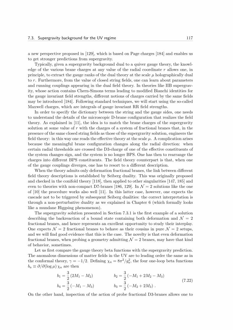
7.3. Supergravity background for the UV regime 117
a new perspective proposed in [129], which is based on Page charges [184] and enables usto get stronger predictions from supergravity.
Typically, given a supergravity background dual to a quiver gauge theory, the knowl-edge of the various brane charges at any value of the radial coordinate r allows one, inprinciple, to extract the gauge ranks of the dual theory at the scale µ holographically dualto r. Furthermore, from the value of closed string fields, one can learn about parametersand running couplings appearing in the dual field theory. In theories like IIB supergrav-ity, whose action contains Chern-Simons terms leading to modified Bianchi identities forthe gauge invariant field strengths, different notions of charges carried by the same fieldsmay be introduced [184]. Following standard techniques, we will start using the so-calledMaxwell charges, which are integrals of gauge invariant RR field strengths.
In order to specify the dictionary between the string and the gauge sides, one needsto understand the details of the microscopic D-brane configuration that realizes the fieldtheory. As explained in [11], the idea is to match the brane charges of the supergravitysolution at some value of r with the charges of a system of fractional branes that, in thepresence of the same closed string fields as those of the supergravity solution, engineers thefield theory: in this way one reads the effective theory at the scale µ. A complication arisesbecause the meaningful brane configuration changes along the radial direction: whencertain radial thresholds are crossed the D3-charge of one of the effective constituents ofthe system changes sign, and the system is no longer BPS. One has then to rearrange thecharges into different BPS constituents. The field theory counterpart is that, when oneof the gauge couplings diverges, one has to resort to a different description.
When the theory admits only deformation fractional branes, the link between differentfield theory descriptions is established by Seiberg duality. This was originally proposedand checked in the conifold theory [118], then applied to other singularities [147, 185] andeven to theories with non-compact D7-branes [186, 129]. In N = 2 solutions like the oneof [10] the procedure works also well [11]. In this latter case, however, one expects thecascade not to be triggered by subsequent Seiberg dualities: the correct interpretation isthrough a non-perturbative duality as we explained in Chapter 6 (which formally lookslike a mundane Higgsing phenomenon).
The supergravity solution presented in Section 7.3.1 is the first example of a solutiondescribing the backreaction of a bound state containing both deformation and N = 2fractional branes, and hence represents an excellent opportunity to study their interplay.One expects N = 2 fractional branes to behave as their cousins in pure N = 2 setups,and we will find good evidence that this is the case. The novelty is that even deformationfractional branes, when probing a geometry admitting N = 2 branes, may have that kindof behavior, sometimes.
Let us first compare the gauge theory beta functions with the supergravity prediction.The anomalous dimensions of matter fields in the UV are to leading order the same as inthe conformal theory, γ = −1/2. Defining χa = 8π2/g2a, the four one-loop beta functionsba ≡ ∂/∂(log µ)χa are then
b1 =3
2(2M1 −M2) b2 =
3
2(−M1 + 2M2 −M3)
b4 =3
2(−M1 −M3) b3 =
3
2(−M2 + 2M3) .
(7.22)
On the other hand, inspection of the action of probe fractional D3-branes allows one to

118 Chapter 7. Cascades of mixed kind and interplay of various fractional branes
find the dictionary between the gauge couplings and the integrals of B2 on the correspond-ing shrinking 2-cycles [158, 70, 102, 128].4 With the conventions laid out in appendix A,the dictionary is easily found to be
χ2 + χ3 =1
2πα′gs
∫
C2
B2 χ1 + χ3 =1
2πα′gs
∫
CCF
B2
χ1 + χ2 =1
2πα′gs
∫
C4
B2 χ1 + χ2 + χ3 + χ4 =2π
gs,
(7.23)
with a radius-energy relation in the UV region r/α′ = µ, like in the conformal case.Recall that CCF = C2 + C4 − 2Cα.
Integrating the NSNS 3-form given in eq. (7.9) one gets for the B2 field
B2 =3
2α′gs log
r
r0
[
(M1 −M2 +M3)ωCF2 + 2π(−M1 +M2 +M3)ω
(p)2
+ 2π(M1 +M2 −M3)ω(q)2
]
+ πα′[
aCF ωCF2 + 4π(a2 ω
(p)2 + a4 ω
(p)4 )]
, (7.24)
where aCF , a2, a4 are integration constants. This implies that
1
2πα′gs
∫
CCF
B2 = 3 (M1 −M2 +M3) logr
r0+
2π
gsaCF
1
2πα′gs
∫
C2
B2 =3
2(−M1 +M2 +M3) log
r
r0+
2π
gsa2
1
2πα′gs
∫
C4
B2 =3
2(M1 +M2 −M3) log
r
r0+
2π
gsa4 .
(7.25)
The three integration constants aCF , a2, a4 correspond to the periods of B2 at r = r0,the latter having being chosen to be the value of the holographic coordinate where theeffective D3-brane charge is N , see the discussion after eq. (7.20). We can think of it asa UV cut-off for the dual gauge theory, i.e. the scale where the dual UV bare Lagrangianis defined. Then the integration constants fix, through eqs. (7.23), the bare couplings ofthe dual non-conformal gauge theory. It is easy to check that the logarithmic derivativesof (7.25) give exactly the same beta functions as the field theory computation in (7.22).
As generically happens in supergravity solutions dual to non-conformal theories, theMaxwell D3-charge runs. It is easily computed from eq. (A.4) and (7.21) to be in ourcase
QD3(r) = N +3gs2π
[M2
1 +M22 +M2
3 −M1M2 −M2M3
]log
r
r0. (7.26)
As in [118], the periods of B2 are no more periodic variables in the non-conformal super-gravity solutions. One should then investigate what the shift in QD3(r) is once we movein the radial direction from r down to r′, where ∆r = r − r′ > 0 is the minimal radiusshift for which all the periods of B2 on Cα, C2, C4 change by an integer (in units of 4π2α′).The shift in QD3(r) should then be compared against the gauge theory expectation for
4Such formula apply in the UV of the supergravity solution because the superpotential coupling is ata quasi-fixed point, as explained in Chapter 5.

7.3. Supergravity background for the UV regime 119
1
2
3
4
7 1234568...
Figure 7.4: Example of the pattern of the cascade of Seiberg dualities for ranks (N + P,N,N +P,N) as derived from the field theory. Black numbers indicate Seiberg dualities, performed ongauge groups with diverging couplings. Inverse squared gauge couplings are plotted versus thelogarithm of the energy scale.
the decrease of the ranks under a specific sequence of cascade steps. What changes aftersuch a sequence are the ranks of the gauge groups, all decreasing by the same integernumber, the theory being otherwise self-similar, and with the initial values of the cou-plings. Sometimes a cyclic permutation of the gauge group factors is also needed, as in[118]. We will call such a sequence of cascade steps a quasi-period.
We are now ready to check the supergravity predictions against the field theory cas-cade in some simple cases. We consider three examples with deformation fractional branesonly, where the RG flow can be followed by performing successive Seiberg dualities, whilein the fourth example below we need an N = 2 duality at some steps of the cascade.
1. (N + P,N,N + P,N)This theory is the daughter of the duality cascade discussed in [118]. There are P
deformation branes of type (1, 0, 1, 0) (corresponding to D5-branes wrapped over CCF ).We get for the charge and the periods
QD3(r) = N +3gs4π
4P 2 logr
r0
bCα = −3gs4π
2P logr
r0+ aα , bC2 = a2 , bC4 = a4 ,
(7.27)
where aCF = a2 + a4 − 2aα and bCi are the periods of B2 along the cycle Ci in unitsof 4π2α′. From the above equation we see that r′ = r exp[−4π/(6gsP )], and under thisradial shift QD3(r
′) = QD3(r) − 2P . This matches with the gauge theory expectationssince the theory is quasi-periodic with a shift N → N − 2P , which is obtained after foursubsequent Seiberg dualities on the different gauge groups. See Figure 7.4 for an explicitexample of the RG flow computed in field theory, for some values of the bare couplings.
120 Chapter 7. Cascades of mixed kind and interplay of various fractional branes
12345678910...
1
4
2
3
Figure 7.5: Example of the pattern of the cascade of Seiberg dualities for ranks (N+P,N,N,N)as derived from the field theory.
Obviously, for any cyclic permutation of the above rank assignment we have the samestory.
2. (N + P,N,N,N)
QD3(r) = N +3gs4π
2P 2 logr
r0
bCα = −3gs4π
P logr
r0+ aα , bC2 = −3gs
4πP log
r
r0+ a2 , bC4 =
3gs4π
P logr
r0+ a4 .
(7.28)
From the above equation we see that r′ = r exp[−4π/(3gsP )] and consequently QD3(r′) =
QD3(r)− 2P . This matches again with gauge theory expectations. Although the quiverlooks self-similar after four Seiberg dualities, the theory is not: the gauge couplingsreturn to their original values only after eight Seiberg dualities, as shown in Figure 7.5.Hence in this case a quasi-period needs eight dualities and the shift in the ranks is indeedN → N − 2P . Again, similar conclusions hold for any cyclic permutations of the aboverank assignment.
3. (N +Q,N +Q,N +Q,N)
QD3(r) = N +3gs4π
2Q2 logr
r0
bCα = aα , bC2 =3gs4π
Q logr
r0+ a2 , bC4 =
3gs4π
Q logr
r0+ a4 .
(7.29)
Here, r′ = r exp[−4π/(3gsQ)] and QD3(r′) = QD3(r)−2Q. A quasi-period requires eight
Seiberg dualities and again agrement with field theory expectations is found. Notice thatthis theory appears along the RG flow of the theory (N ′, N ′, N ′, N ′ +Q).

7.3. Supergravity background for the UV regime 121
4. (N + P,N + P,N,N)
QD3(r) = N +3gs4π
2P 2 logr
r0
bCα =3gs4π
P logr
r0+ aα , bC2 = a2 , bC4 =
3gs4π
2P logr
r0+ a4 .
(7.30)
Here r′ = r exp[−4π/(3gsP )] and QD3(r′) = QD3(r) − 2P . For such N = 2 fractional
branes we have to perform some duality at nodes with adjoints (cfr. the left quiveron Figure 7.7 below), at some step along the cascade. We conjecture that it can beunderstood as some N = 1 generalization of the baryonic root transition found in theN = 2 cascade. Formally its only effect is to change the rank of the gauge group withan adjoint from N + P to N − P . For this reason we will loosely refer to this non-perturbative transition as “Higgsing”. The RG flow is shown in Figure 7.10 (we willexplain how this can be obtained from supergravity below). The quiver looks self-similarafter three Seiberg dualities, which consist of one Seiberg duality on node 1, one Higgsingon node 2 and again one Seiberg duality on node 1. However a quasi-period needs sixdualities, as apparent in Figure 7.10, and the shift in the ranks is N → N − 2P , asexpected.
7.3.3 Page charges and the RG flow from supergravity
There is another way of matching our running supergravity solutions (and more generallytype IIB solutions constructed from fractional branes at conical singularities) with cas-cading field theories. The method was originally proposed in [129], working on ideas in[184]. Instead of using Maxwell charges, which are conserved and gauge invariant but notquantized nor localized, the method is based on Page charges [187] which are conservedand quantized, and therefore more suitable to be identified with gauge ranks, even thoughthey shift under large gauge transformations.
Let C be a formal sum (polyform) of RR potentials C =∑Cp, and F = (d+H3∧)C
the field strength polyform. Suppose we have a Dp-brane, whose dual current (looselyspeaking its Poincare dual) is a (9− p)-form Ω9−p, with world-volume flux F2. Then theEOM/BI for the fluxes read
(d+H3∧)F = eF ∧∑
p
σp 2κ2τp Ω9−p
⇒ dFPage ≡ d(eB2 ∧ F ) = e2πα′F2 ∧
∑
p
σp 2κ2τp Ω9−p ,
(7.31)
where σ1 = σ7 = 1 and σ−1 = σ3 = σ5 = −1. In particular FPage is a closed polyformoutside the branes. Then Maxwell and Page charges are defined as
Maxwell: Qp =σp
2κ2τp
∫
S8−p
F Page: QPagep =σp
2κ2τp
∫
S8−p
eB2 ∧ F . (7.32)
The idea is that it is possible to read the field theory RG flow from supergravitypointwise. At fixed radial coordinate r dual to some scale µ, standard formulæ allow usto compute the gauge couplings from the dilaton and the integrals of B2. Such formulæ
122 Chapter 7. Cascades of mixed kind and interplay of various fractional branes
do not give real couplings in general, but need particular integer shifts of B2, which arelarge gauge transformations. Consequently, Page charges get shifted by some integervalues. Having at hand a dictionary, they are readily mapped to the ranks of the gaugetheory at that scale.
At some specific radii, in order to keep the couplings real, one has to perform afurther large gauge transformation, shifting B2 and therefore ending up with differentranks. These points connect different steps of the cascade and can usually be interpretedin the field theory as Seiberg dualities [118] or non-perturbative Higgsings. In particular,ranks are not continuously varying functions but rather integer discontinuous ones. Thisis not the end of the story: in general the shifts of B2 are not enough to save us fromimaginary couplings, and one is forced to introduce multiple dictionaries. We will seehow everything beautifully merges.
Let us make the point clear using the Klebanov-Strassler cascade [127, 118]. Thefirst step is to identify a dictionary between the field theory ranks and Page charges.An SU(N +M) × SU(N) theory is microscopically engineered with N regular and Mfractional D3-branes at the tip of the conifold, thus from eq. (7.31) QPage3 = N , QPage5 =M . The formulæ for the gauge couplings are
χ1 =2π
gsb χ2 =
2π
gs(1− b) , (7.33)
where χa = 8π2/g2a and a = 1 refers to the larger group, while 4π2α′ b =∫
S2 B2. Fromthe actual UV solution [127], we have (for B2 in some gauge)
b =1
4π2α′
∫
S2
B2 =3gsM
2πlog
r
r0Q3 = −
1
2κ2τ3
∫
T 1,1
F5 = N +3gsM
2
2πlog
r
r0.
(7.34)At any radius/energy scale x ≡ log r/r0 one should perform a large gauge transformationand shift b by some integer ∆b such that χa ≥ 0, compute the Page charges in such agauge, and finally use the dictionary to evaluate the ranks at that scale.
It is easy to evaluate ∆b and QPage3 in this example. They read
∆b = −[3gsM
2πx]
−QPage3 = N −∆bM = N +
[3gsM
2πx]
−M , (7.35)
where the floor function [y]− is the greatest integer less than or equal to y. Applying thealgorithm at any x, we can plot the RG flow of the gauge couplings and the ranks alongit. The result (the famous KS cascade) is depicted in Figure 7.6. Notice that we neverimposed continuity of the gauge couplings (even though it is a well motivated physicalrequirement), nevertheless the supergravity solution predicts it. Moreover it also suggestsa reduction in the gauge group ranks without explaining the corresponding field theorymechanism. It turns out that in this case Seiberg duality can beautifully account for it[118, 85].
We want to apply the same procedure to our class of solutions. In order to do that,however, we need some more machinery. Given a basis of 2-cycles Ci and 3-cycles Aj onradial sections, one defines an intersection matrix
Ci ·Aj = Iij i, j = 1 . . . p , (7.36)

7.3. Supergravity background for the UV regime 123
SU(N) × SU(N − M)Q
Page3 = N − M
SU(N) × SU(N + M)Q
Page3 = N
SU(N + 2M) × SU(N + M)Q
Page3 = N + M
1-1
χ
x0
1
Figure 7.6: Flow in the KS theory as computed with the algorithm. x is in units of 2π/3gsMwhile χ in units of 2π/gs. At integer values of x a large gauge transformation is required. At eachstep the Page D3-charge and the field theory is indicated.
where p is the number of fractional branes. Let (nI) = (#D5i,#D3), I = 1 . . . p + 1 bethe occupation vector, that is the numbers of D5-branes wrapped on Ci and of D3-branes.A dictionary F(m) relates this system to the ranks ra, a = 1 . . . P of the dual gauge theory
ra = [F(m)]aI nI . (7.37)
In general P ≥ p+ 1, but for our non-chiral theory P = p+ 1 and F(m) is invertible. Inthe following i, j = 1 . . . p while I, J, a, b = 1 . . . p + 1. Let (QI) be the vector of Pagecharges
(QI) =(
− 1
2κ2τ5
∫
Aj
F3 , −1
2κ2τ3
∫
FPage5
)
, (7.38)
then the Bianchi identity eq. (7.31) implies that Qj = −Itji ni. Introducing the matrix
I = diag(−It, 1) we can write: QI = IIJ nJ . It follows that (suppressing indices)
r =(
F(m) I−1)
Q . (7.39)
The formulæ relating the gauge couplings to the supergravity solution can be derivedby considering the worldvolume action of probe D3- and wrapped D5-branes [185]. Letχa = 8π2/g2a as before. Considering D3-branes one concludes that
∑χa = 2π/gs; then
the integral of B2 on some 2-cycle Cj is related to the gauge coupling on the probe D5-brane, which is itself related to the sum of the χ’s corresponding to the ranks increasedby the D5, as in (7.23). Defining the vector
(BI) =( 1
4π2α′
∫
Ci
B2 , 1)
(7.40)
one can summarize the relations by
2π
gsB = F t(m) χ ⇒ χ =
2π
gsF−1t(m) B . (7.41)
124 Chapter 7. Cascades of mixed kind and interplay of various fractional branes
Under large gauge transformations the integrals of B2 change by integer amounts, thusthe first p components of the vector B undergo a particular shift Bi → Bi +Zi, for someZi ∈ Z. As a result the Page D3-charge is shifted by
∆QPage3 = − 1
2κ2τ3
∫
∆B2 ∧ F3 = Qj (I−1)jk Zk , (7.42)
while the inferred gauge couplings change according to eq. (7.41).We now apply the algorithm to our solutions (7.9), where the integrals of B2 are (7.25),
for some values of the charges (equivalently for some Mi’s). Using the basis C2, C4, Cαfor the 2-cycles and A2, A4, ACF for the 3-cycles, the intersection matrix Iij is givenby
Iij =
−2 0 00 −2 0−1 −1 1
(7.43)
as in (F.39), while the dictionary [F(1)]aI derived in section 7.2.2 (see Table (7.6)), refer-ring to the central quiver in Figure 7.7, is reported in Figure 7.8. One quickly discoversthat, for generic values of the integration constants ai and of the radial coordinate r,there is no gauge transformation that produces positive χa in eq. (7.41).
One is led to the conclusion that multiple dictionaries are needed. This had to beexpected since performing any Seiberg duality on the central quiver in Figure 7.7 one ob-tains the lateral quivers (depending on the node chosen), which are substantially differentand cannot be described by the same dictionary, even up to reshuffling of the nodes.
It turns out that even two dictionaries are not enough in our case. We provide a setof six dictionaries such that, at any energy, for one and only one dictionary there is onelarge gauge transformation that gives non-negative χa, see Figure 7.8.
The dictionaries besides F(1) are obtained from it through formal Seiberg dualities.Consider a system with occupation vector n = (n1, n2, n3, N). Start with the centralquiver where the ranks are given by eq. (7.37) using F(1). Then a formal Seiberg dualityon one node gives a new quiver with new ranks (and superpotential), from which a newdictionary F(m) is directly read. Actually there is an ambiguity because the number ofD3-branes N could have changed in the process (but not the other charges) and thenone is free to add lines of 1’s to any of the first three columns. One can show that thephysical result, that is the gauge couplings and ranks in the correct gauge of B2, is notaffected. In our case, a Seiberg duality on node 1 gives F(4), on node 2 F(6), on node 3F(3), on node 4 F(5) and on two opposite nodes F(2).
We can finally apply the algorithm at any radius x ≡ log r/r0, that is:
• find a dictionary in the set F(m) and a large gauge transformation Bi(x) →Bi(x) + Zi such that, according to eq. (7.41), χI ≥ 0 ∀I. It turns out that thereis always one and only one solution;5
• compute the D3-brane Page charge in this gauge, using eq. (7.42) (D5-brane chargesare invariant);
5To be precise, when one of the χI vanishes there are two dictionaries (with their gauges) that do thejob. At these radii there is the transition between the validity domains of two different field theory duals.

7.3. Supergravity background for the UV regime 125
Figure 7.7: Seiberg dual quivers. The central quiver is the most extensively discussed one in thischapter. The left quiver is obtained with a Seiberg duality on node 1 or 3, while the right one onnode 2 or 4.
F(3) =
0 1 0 11 1 1 10 1 1 10 0 0 1
F(1) =
0 1 0 11 1 1 11 0 0 10 0 0 1
F(5) =
0 1 0 11 1 1 11 0 0 11 1 0 1
F(4) =
1 0 1 11 1 1 11 0 0 10 0 0 1
F(2) =
1 0 1 11 1 1 10 1 1 10 0 0 1
F(6) =
0 1 1 10 0 0 11 0 1 10 0 1 1
Figure 7.8: A set of six dictionaries for the orbifolded conifold theory. F(3), F(4) refer to the leftquiver, with adjoints on nodes 2-4; F(1), F(2) refer to the central quiver, without adjoints; F(5),F(6) refer to the right quiver, with adjoints on nodes 1-3. The four columns represent the nodesactivated by a D5-brane on C2, C4, Cα and a D3-brane respectively.
• use the dictionary and the charges in eq. (7.39) to evaluate the ranks at that scalein the corresponding quiver.
As a result, one can plot the gauge couplings along the flow and keep track of the variousfield theory descriptions.
It is clear that the transition radii between two different descriptions (dictionaries)occur when one of the χI vanishes. But in principle there is no reason why one shouldexpect, from the procedure above, continuous couplings at the transition points. Surpris-ingly enough, it turns out that the resulting coupling are indeed continuous. Some plotswith explanation are in Figures 7.9, 7.10, 7.11, 7.12 (obtained via a mathematica code).In the following, we comment on interesting examples.
1. (N + P,N,N + P,N)
The RG flow, as computed from supergravity with the algorithm above, is plotted inFigure 7.9 (for P = 1 and some typical choice of the integration constants a2, a4, aα andthe starting radius x = log r/r0). It precisely matches with the field theory expectations,with respect to both gauge couplings and ranks at any step. All transition points canbe interpreted by means of a single Seiberg duality, as the prototypical example in [118].Notice that the integral of B2 on C2 and C4 is constant and generically not integer.
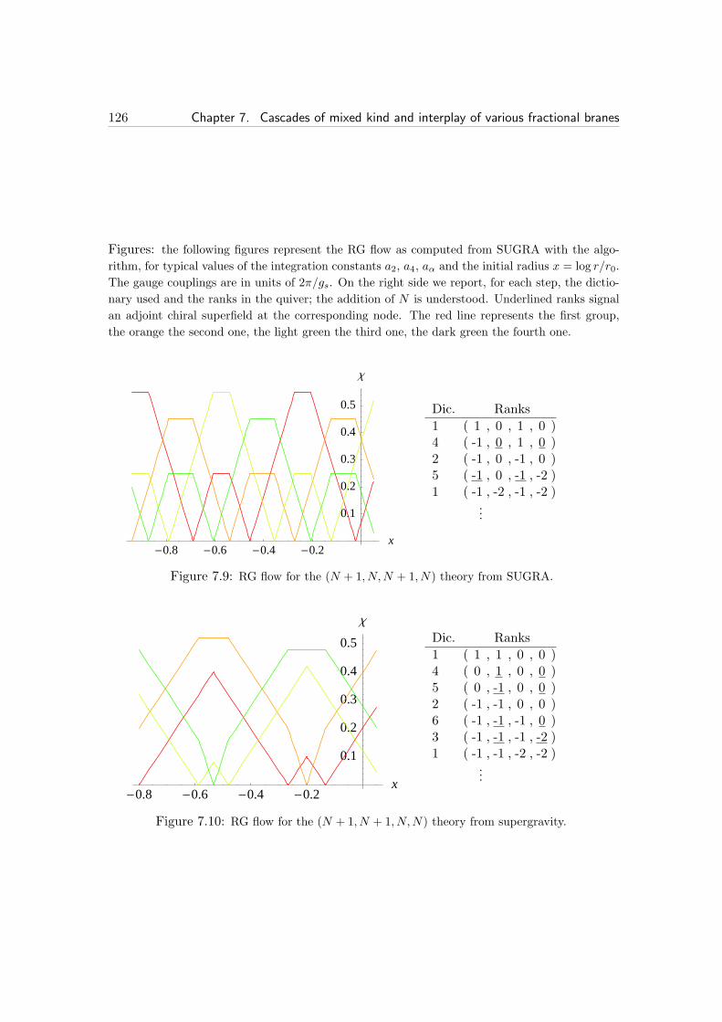
126 Chapter 7. Cascades of mixed kind and interplay of various fractional branes
Figures: the following figures represent the RG flow as computed from SUGRA with the algo-
rithm, for typical values of the integration constants a2, a4, aα and the initial radius x = log r/r0.
The gauge couplings are in units of 2π/gs. On the right side we report, for each step, the dictio-
nary used and the ranks in the quiver; the addition of N is understood. Underlined ranks signal
an adjoint chiral superfield at the corresponding node. The red line represents the first group,
the orange the second one, the light green the third one, the dark green the fourth one.
-0.8 -0.6 -0.4 -0.2x
0.1
0.2
0.3
0.4
0.5
Χ
Dic. Ranks
1 ( 1 , 0 , 1 , 0 )4 ( -1 , 0 , 1 , 0 )2 ( -1 , 0 , -1 , 0 )5 ( -1 , 0 , -1 , -2 )1 ( -1 , -2 , -1 , -2 )
...
Figure 7.9: RG flow for the (N + 1, N,N + 1, N) theory from SUGRA.
-0.8 -0.6 -0.4 -0.2x
0.1
0.2
0.3
0.4
0.5
Χ
Dic. Ranks
1 ( 1 , 1 , 0 , 0 )4 ( 0 , 1 , 0 , 0 )5 ( 0 , -1 , 0 , 0 )2 ( -1 , -1 , 0 , 0 )6 ( -1 , -1 , -1 , 0 )3 ( -1 , -1 , -1 , -2 )1 ( -1 , -1 , -2 , -2 )
...
Figure 7.10: RG flow for the (N + 1, N + 1, N,N) theory from supergravity.
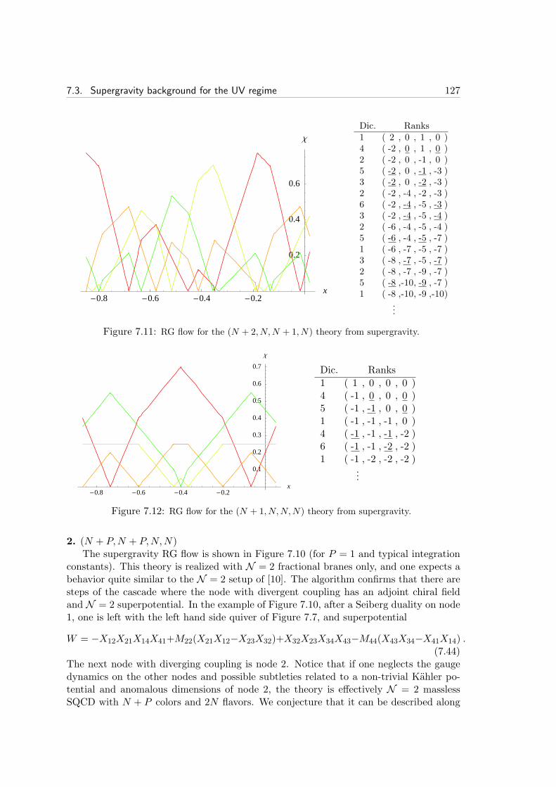
7.3. Supergravity background for the UV regime 127
-0.8 -0.6 -0.4 -0.2x
0.2
0.4
0.6
Χ
Dic. Ranks1 ( 2 , 0 , 1 , 0 )4 ( -2 , 0 , 1 , 0 )2 ( -2 , 0 , -1 , 0 )5 ( -2 , 0 , -1 , -3 )3 ( -2 , 0 , -2 , -3 )2 ( -2 , -4 , -2 , -3 )6 ( -2 , -4 , -5 , -3 )3 ( -2 , -4 , -5 , -4 )2 ( -6 , -4 , -5 , -4 )5 ( -6 , -4 , -5 , -7 )1 ( -6 , -7 , -5 , -7 )3 ( -8 , -7 , -5 , -7 )2 ( -8 , -7 , -9 , -7 )5 ( -8 ,-10, -9 , -7 )1 ( -8 ,-10, -9 ,-10)
...
Figure 7.11: RG flow for the (N + 2, N,N + 1, N) theory from supergravity.
-0.8 -0.6 -0.4 -0.2x
0.1
0.2
0.3
0.4
0.5
0.6
0.7
Χ
Dic. Ranks
1 ( 1 , 0 , 0 , 0 )4 ( -1 , 0 , 0 , 0 )5 ( -1 , -1 , 0 , 0 )1 ( -1 , -1 , -1 , 0 )4 ( -1 , -1 , -1 , -2 )6 ( -1 , -1 , -2 , -2 )1 ( -1 , -2 , -2 , -2 )
...
Figure 7.12: RG flow for the (N + 1, N,N,N) theory from supergravity.
2. (N + P,N + P,N,N)The supergravity RG flow is shown in Figure 7.10 (for P = 1 and typical integration
constants). This theory is realized with N = 2 fractional branes only, and one expects abehavior quite similar to the N = 2 setup of [10]. The algorithm confirms that there aresteps of the cascade where the node with divergent coupling has an adjoint chiral fieldand N = 2 superpotential. In the example of Figure 7.10, after a Seiberg duality on node1, one is left with the left hand side quiver of Figure 7.7, and superpotential
W = −X12X21X14X41+M22(X21X12−X23X32)+X32X23X34X43−M44(X43X34−X41X14) .(7.44)
The next node with diverging coupling is node 2. Notice that if one neglects the gaugedynamics on the other nodes and possible subtleties related to a non-trivial Kahler po-tential and anomalous dimensions of node 2, the theory is effectively N = 2 masslessSQCD with N + P colors and 2N flavors. We conjecture that it can be described along
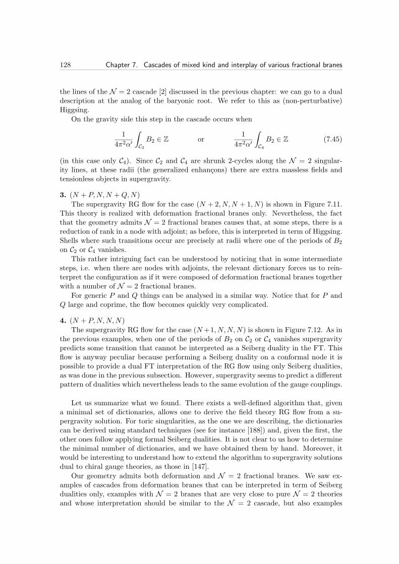
128 Chapter 7. Cascades of mixed kind and interplay of various fractional branes
the lines of the N = 2 cascade [2] discussed in the previous chapter: we can go to a dualdescription at the analog of the baryonic root. We refer to this as (non-perturbative)Higgsing.
On the gravity side this step in the cascade occurs when
1
4π2α′
∫
C2
B2 ∈ Z or1
4π2α′
∫
C4
B2 ∈ Z (7.45)
(in this case only C4). Since C2 and C4 are shrunk 2-cycles along the N = 2 singular-ity lines, at these radii (the generalized enhancons) there are extra massless fields andtensionless objects in supergravity.
3. (N + P,N,N +Q,N)
The supergravity RG flow for the case (N + 2, N,N + 1, N) is shown in Figure 7.11.This theory is realized with deformation fractional branes only. Nevertheless, the factthat the geometry admits N = 2 fractional branes causes that, at some steps, there is areduction of rank in a node with adjoint; as before, this is interpreted in term of Higgsing.Shells where such transitions occur are precisely at radii where one of the periods of B2
on C2 or C4 vanishes.
This rather intriguing fact can be understood by noticing that in some intermediatesteps, i.e. when there are nodes with adjoints, the relevant dictionary forces us to rein-terpret the configuration as if it were composed of deformation fractional branes togetherwith a number of N = 2 fractional branes.
For generic P and Q things can be analysed in a similar way. Notice that for P andQ large and coprime, the flow becomes quickly very complicated.
4. (N + P,N,N,N)
The supergravity RG flow for the case (N+1, N,N,N) is shown in Figure 7.12. As inthe previous examples, when one of the periods of B2 on C2 or C4 vanishes supergravitypredicts some transition that cannot be interpreted as a Seiberg duality in the FT. Thisflow is anyway peculiar because performing a Seiberg duality on a conformal node it ispossible to provide a dual FT interpretation of the RG flow using only Seiberg dualities,as was done in the previous subsection. However, supergravity seems to predict a differentpattern of dualities which nevertheless leads to the same evolution of the gauge couplings.
Let us summarize what we found. There exists a well-defined algorithm that, givena minimal set of dictionaries, allows one to derive the field theory RG flow from a su-pergravity solution. For toric singularities, as the one we are describing, the dictionariescan be derived using standard techniques (see for instance [188]) and, given the first, theother ones follow applying formal Seiberg dualities. It is not clear to us how to determinethe minimal number of dictionaries, and we have obtained them by hand. Moreover, itwould be interesting to understand how to extend the algorithm to supergravity solutionsdual to chiral gauge theories, as those in [147].
Our geometry admits both deformation and N = 2 fractional branes. We saw ex-amples of cascades from deformation branes that can be interpreted in term of Seibergdualities only, examples with N = 2 branes that are very close to pure N = 2 theoriesand whose interpretation should be similar to the N = 2 cascade, but also examples
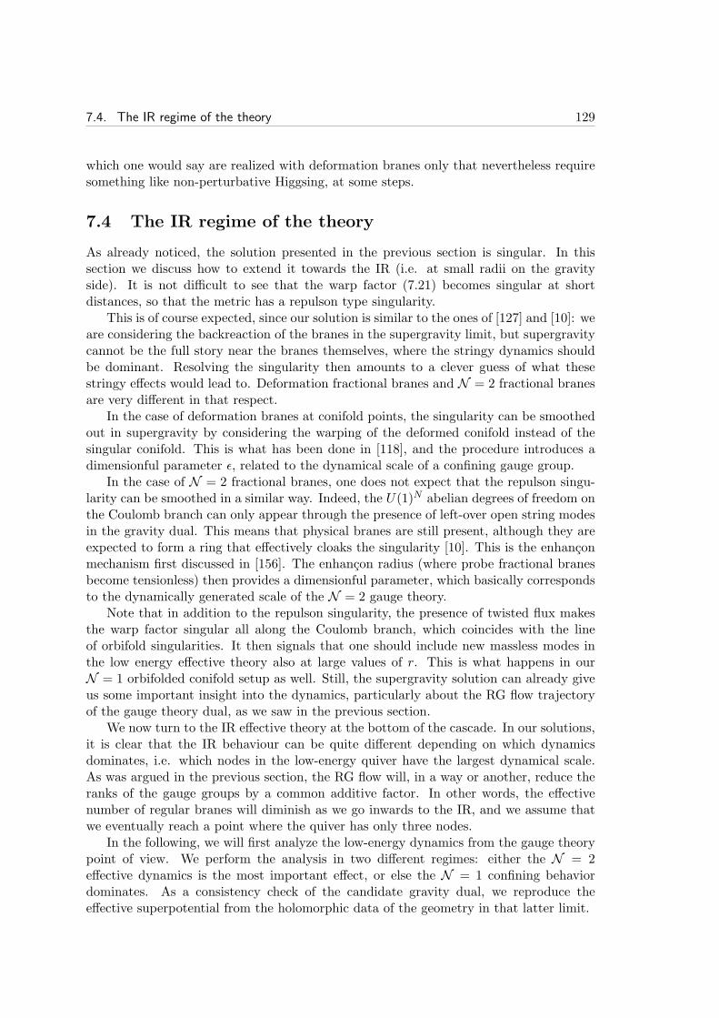
7.4. The IR regime of the theory 129
which one would say are realized with deformation branes only that nevertheless requiresomething like non-perturbative Higgsing, at some steps.
7.4 The IR regime of the theory
As already noticed, the solution presented in the previous section is singular. In thissection we discuss how to extend it towards the IR (i.e. at small radii on the gravityside). It is not difficult to see that the warp factor (7.21) becomes singular at shortdistances, so that the metric has a repulson type singularity.
This is of course expected, since our solution is similar to the ones of [127] and [10]: weare considering the backreaction of the branes in the supergravity limit, but supergravitycannot be the full story near the branes themselves, where the stringy dynamics shouldbe dominant. Resolving the singularity then amounts to a clever guess of what thesestringy effects would lead to. Deformation fractional branes and N = 2 fractional branesare very different in that respect.
In the case of deformation branes at conifold points, the singularity can be smoothedout in supergravity by considering the warping of the deformed conifold instead of thesingular conifold. This is what has been done in [118], and the procedure introduces adimensionful parameter ǫ, related to the dynamical scale of a confining gauge group.
In the case of N = 2 fractional branes, one does not expect that the repulson singu-larity can be smoothed in a similar way. Indeed, the U(1)N abelian degrees of freedom onthe Coulomb branch can only appear through the presence of left-over open string modesin the gravity dual. This means that physical branes are still present, although they areexpected to form a ring that effectively cloaks the singularity [10]. This is the enhanconmechanism first discussed in [156]. The enhancon radius (where probe fractional branesbecome tensionless) then provides a dimensionful parameter, which basically correspondsto the dynamically generated scale of the N = 2 gauge theory.
Note that in addition to the repulson singularity, the presence of twisted flux makesthe warp factor singular all along the Coulomb branch, which coincides with the lineof orbifold singularities. It then signals that one should include new massless modes inthe low energy effective theory also at large values of r. This is what happens in ourN = 1 orbifolded conifold setup as well. Still, the supergravity solution can already giveus some important insight into the dynamics, particularly about the RG flow trajectoryof the gauge theory dual, as we saw in the previous section.
We now turn to the IR effective theory at the bottom of the cascade. In our solutions,it is clear that the IR behaviour can be quite different depending on which dynamicsdominates, i.e. which nodes in the low-energy quiver have the largest dynamical scale.As was argued in the previous section, the RG flow will, in a way or another, reduce theranks of the gauge groups by a common additive factor. In other words, the effectivenumber of regular branes will diminish as we go inwards to the IR, and we assume thatwe eventually reach a point where the quiver has only three nodes.
In the following, we will first analyze the low-energy dynamics from the gauge theorypoint of view. We perform the analysis in two different regimes: either the N = 2effective dynamics is the most important effect, or else the N = 1 confining behaviordominates. As a consistency check of the candidate gravity dual, we reproduce theeffective superpotential from the holomorphic data of the geometry in that latter limit.

130 Chapter 7. Cascades of mixed kind and interplay of various fractional branes
Figure 7.13: The 3-node quiver that corresponds to the IR bottom of the cascade.
We eventually consider the equations determining the warp factor. The latter is re-lated to data encoded in the full Kahler potential of the gauge theory. Hence, computingthe warp factor would be the main challenge in order to gather new dynamical infor-mation on the low-energy theory. To do that, the two limits in which the dynamics ispredominantly confining or N = 2 are quite different. In the latter case, we will arguethat the enhancon is so large that a possible local deformation of the geometry wouldbe irrelevant, and so the UV solution presented in the previous section is basically thecorrect gravity dual up to the enhancon radius. When instead the confining dynamics isthe strongest, one expects to have a gravity dual consisting of the orbifold of the deformedconifold, with singularities along the orbifold fixed line. We must anticipate that we willstop short of actually computing the warp factor in that case.
7.4.1 Gauge theory IR dynamics
In this subsection we perform the gauge theory analysis for the low-energy behavior ofa generic 3-node quiver, see Figure 7.13. It will often prove useful to actually think ofmoduli spaces in terms of mobile (fractional) branes, so we will freely make reference tothis interpretation even in the course of the purely gauge theoretic analysis.
Let us call Λi the dynamically generated scale of the i-th node of the quiver, withi = 1, 2, 3. We consider two qualitatively different regimes.
First we analyze the regime Λ2 ≫ Λ1,3, where the dominant quantum effects comefrom the second node. As we will see, for M2 < M1 +M3, there is no deformation of the(mesonic) moduli space, which itself corresponds to having a stack of N = 2 fractionalbranes on their Coulomb branch. For M2 > M1+M3, we find a runaway behavior on theCoulomb branch. This is interpreted in the gravity dual as a fully regular deformationof the geometry in the presence of N = 2 fractional branes. Indeed, in this case theexceptional cycle the branes wrap is blown-up and minimizes its volume at infinity: theN = 2 branes are pushed away.
Secondly, the regime Λ2 ≪ Λ1,3 is analyzed (a similar analysis was performed in theappendix of [182]). One finds gaugino condensation for both nodes one and three, withS1 = S3. On the dual geometric side, the deformation branes trigger a geometric tran-sition that still preserves an orbifold singularity line in the resulting deformed geometry.The singularity line can accommodate some left over N = 2 branes which explore theirmoduli space.
Regime Λ2 ≫ Λ1,3
In this regime, the only gauge dynamics we take into account is the one of the secondnode. The quiver configuration is (M1,M2,M3, 0) with 3M2 > M1 +M3, so that node 2

7.4. The IR regime of the theory 131
has a strongly coupled IR dynamics and it makes sense to neglect the scales of the othernodes as a first approximation.
The tree level superpotential is
Wtree = λX12X23X32X21 (7.46)
and the quantum corrected one is
W =Wtree − (M1 −M2 +M3)
(
detKΛ3M2−M1−M32
) 1M1−M2+M3
. (7.47)
If M2 > M1 +M3, this is the familiar Affleck-Dine-Seiberg (ADS) superpotential [138],while if M2 < M1+M3, it is the effective superpotential for the free Seiberg dual mesonsand vanishing dual quark VEVs.6
The meson matrix for the second node is
K ≡(X12X21 X12X23
X32X21 X32X23
)
≡(K11 K13
K31 K33
)
. (7.48)
Let us denote
S2 ≡(
detKΛ3M2−M1−M32
) 1M1−M2+M3
. (7.49)
We want to determine the moduli space of such a theory. Considering the effectivesuperpotential in terms of the mesons, one has the following F-flatness conditions
S2(K−1)11 = 0 = S2(K−1)33
λK31 − S2(K−1)31 = 0 = λK13 − S2(K−1)13 (7.50)
This impliesM1S2 =M3S2 . (7.51)
We must then have7 that S2 = 0, which implies that K13 and K31 must vanish, anddetK = detK11 detK33. When M2 < M1 + M3 the constraint S2 = 0 means thatdetK = 0. Using the gauge freedom of the first and third nodes, the general solutionconsists of K diagonal with M2 non-vanishing eigenvalues. There are as many distinctsuch solutions as there are possibilities of choosing M2 out of the M1 + M3 N = 2subquiver configurations (1, 1, 0, 0) or (0, 1, 1, 0).
When we have instead M2 > M1 + M3, there is an ADS superpotential, and theconstraint on the mesons become
detK = detK11 detK33 →∞ . (7.52)
6In principle, we should worry about additional baryonic directions in the effective dynamics. Theirfully quantum analysis is beyond the scope of the present analysis, however both the classical gaugetheory analysis of the higgsing patterns and their interpretation in terms of brane motions hint that thestatements concerning the mesonic VEVs should not be modified.
7UnlessM1 =M3, where we have another possible solution: K11 = K33 = 0 and S2 = Λ32(λΛ2)
M1
M2−M1 ,presumably related to a non-Coulomb branch.

132 Chapter 7. Cascades of mixed kind and interplay of various fractional branes
This corresponds to a runaway behavior of the N = 2 brane configuration (the samephenomenon was observed in [189, 190]). Indeed, after all the N = 2 configurations havebeen accounted for (by moving on the Coulomb branch), there remains the configuration(0,M2 −M1 −M3, 0, 0), that confines, and we know that this should correspond to thefollowing deformation of the geometry seen by D3-branes
(z1z2 − S2)z1z2 = xy . (7.53)
This space only has a singularity at the origin, so that the Coulomb branch (whichcorresponds to a singularity line in the orbifolded conifold) is lifted, the supersymmetricvacua being preserved only at infinity. Geometrically what happens is that the N = 2branes become non-BPS, as they wrap a blown-up cycle, and they can only minimizetheir tension by moving off to infinity.
Regime Λ2 ≪ Λ1,3
In the regime Λ1,3 ≫ Λ2, gaugino condensation at the first and third nodes is the dominanteffect in the IR. This corresponds to a complex structure deformation of the geometry,induced by the deformation fractional branes. We again consider the quiver configuration(M1,M2,M3, 0) with tree level superpotential (7.46).
Let us restrict to the case where M2 < M1,M3.8 The first and the third gauge groups
develop an ADS superpotential at the quantum level, while the second gauge group canbe considered classical. In term of the mesons M = X21X12 and N = X23X32 of thefirst and third nodes respectively (which are both M2 ×M2 matrices in the adjoint plussinglet of the second node), the full effective superpotential reads
W = λMN +(M1−M2)
(
Λ3M1−M21
detM
) 1M1−M2
+(M3−M2)
(
Λ3M3−M23
detN
) 1M3−M2
. (7.54)
Instead of solving for the extrema of the above superpotential, we find it useful to firstintegrate in the glueball superfields for the two confining gauge groups. We are alsomotivated in doing this by the approach which uses the Gukov-Vafa-Witten (GVW) [191]superpotential to make the link between the gauge theory and the geometrical quantities,and which will be pursued in section 7.4.2. We thus obtain
W = λMN+(M1−M2)S1−S1 logSM1−M21 detMΛ3M1−M21
+(M3−M2)S3−S3 logSM3−M23 detNΛ3M3−M23
,
(7.55)which is a Taylor-Veneziano-Yankielowicz (TVY) [192] kind of superpotential. Of course,extremizing with respect to S1 and S3 will lead us back to the previous ADS-like super-potential. However let us extremize with respect to all fields together
λN = S1M−1, λM = S3N−1, (7.56)
8If M2 > M1,M3, two Seiberg dualities on nodes one and three bring us back to the case analyzedpreviously because we can assume that the dual scales are such that Λ1,3 ≪ Λ2. If M1 > M2 > M3, it ispossible to show that the system has a runaway behavior.
7.4. The IR regime of the theory 133
logSM1−M21 detMΛ3M1−M21
= 0, logSM3−M23 detNΛ3M3−M23
= 0 . (7.57)
The above equations imply thatM is proportional to the inverse of N , and that
S1 = S3 ≡ S =(
λM2Λ3M1−M21 Λ3M3−M2
3
) 1M1−M2+M3 . (7.58)
This of course implies that also detM is fixed, while the moduli space is spanned by thevalues ofM subject to this constraint. Once the effective N = 2 dynamics of the SU(M2)gauge group is taken into account, the moduli space reduces to the M2 − 1 directions inthe Cartan subalgebra.
Let us also consider two limiting cases. IfM1 =M2 =M3 ≡M , one can check that themesonic and the baryonic branches decouple. On the mesonic branch, the superpotential(7.55) is correct and the solution to its extremization is
detM = Λ2M1 , detN = Λ2M
3 , S1 = S3 =(λMΛ2M
1 Λ2M3
) 1M . (7.59)
The dynamics is essentially the same as before. Note that the Si act effectively as La-grange multipliers, and their being non zero is a signal of the decoupling of the mesonicfrom the baryonic branch. This was the case of most interest in [182].
The other limiting case isM2 = 0. Here there are no mesonsM and N , and hence nocoupling between nodes one and three. We just have a sum of two Veneziano-Yankielowiczsuperpotentials [193] for two decoupled SYM theories. Consistently, we obtain uponextremization
S1 =(
Λ3M11
) 1M1 , S3 =
(
Λ3M33
) 1M3 . (7.60)
In this case, the two VEVs Si are independent. It corresponds to a generic deformationof the geometry, as reviewed in appendix F.2.
7.4.2 The Gukov-Vafa-Witten superpotential
In this subsection, we make an important consistency check of our gauge/gravity set upby matching the GVW superpotential [191] to the gauge theory effective superpotentialconsidered in the previous subsection.
It is well known that Calabi-Yau compactification of type IIB in the presence of fluxeshelps to restrict the allowed values of the complex structure moduli. The dynamics ofthese moduli can be encoded in an effective superpotential WGVW for the resulting fourdimensional supergravity. In the gauge/gravity correspondence setup, WGVW can alsobe computed, provided we fix some boundary conditions at infinity on the non-compactCY we are using. It can be written as
WGVW =i
2πgsα′4
∫
M6
G3 ∧ Ω , (7.61)
where Ω is the holomorphic 3-form. One can then compare this WGVW superpotential tothe dual gauge theory superpotential, since they are expected to agree on-shell.9
9Remark that WGVW is a supergravity superpotential, in particular dWGVW = 0 =WGVW on super-symmetric compactifications. To decouple gravity we must consider non-compact manifolds and accord-ingly on the dual gauge theory side we only have dW = 0.

134 Chapter 7. Cascades of mixed kind and interplay of various fractional branes
In the absence of brane sources, the G3 flux is closed and depends only on the coho-mology class of G3. Adding some D5-brane sources for G3, however, one must keep trackof the position of these branes [174, 194, 195]. Separating G3 into a bulk contribution (i.e.closed part) Gb
3 and a contribution from the sources Gs3, and using Riemann relations forthe closed part, one has
WGVW =i
2πgsα′4
∑
j
(∫
Aj
Gb3
∫
Bj
Ω−∫
Bj
(Gb3 +Gs
3)
∫
Aj
Ω)
− 2πi
α′3
∑
N = 2 branes
∫
Ξ3
Ω ,
(7.62)where Ξ3 is a 3-chain that extends from the 2-cycle wrapped by the D5-brane to somereference 2-cycle near infinity.10
Let us now computeWGVW in our orbifolded conifold geometry. We consider a genericsmooth deformation, with the two complex structure parameters ǫ1, ǫ3 arbitrary, see(F.36), and we take the limit where the wrapped D5-branes are far from the deformationnear the tip. With an obvious linear change of coordinates, the geometry is defined by
xy − (u2 − v2 + ǫ1)(u2 − v2 + ǫ3) = 0 (7.63)
in C4 ∼= x, y, u, v. The holomorphic 3-form Ω is given by
Ω =1
2π2du ∧ dv ∧ dx
x. (7.64)
We obtain the usual results for the periods of Ω on the A and B cycles (see appendicesF.2 and F.4 for more details)
∫
Aj
Ω = ǫj , and
∫
Bj
Ω =ǫj2πi
log
(ǫi
4ev20
)
+ regular , (7.65)
where v = v0 is a cut-off for the non-compact B-cycles. The contribution to (7.62) comingfrom D5-branes wrapped on C2 is computed in appendix F.4 : for a D5-brane located atv = ξ, in the limit |v0|2 , |ξ|2 ≫ |ǫk|, we have the simple result
∫
Ξ3
Ω = − 1
2πi(ǫ1 − ǫ3) log
ξ
v0+O
( ǫ2
ξ4
)
. (7.66)
Let us now consider the following F3 fluxes
− 1
4π2gsα′
∫
A1
Gb3 =M1, − 1
4π2gsα′
∫
A3
Gb3 =M3 −M2 . (7.67)
This means we assume that M1 and M3 − M2 D5-branes that were wrapped on the2-cycles C1 and C3, see eq. (F.35), have undergone geometric transition independently.11
10For an intuitive feel for the meaning of that formula, one can think of a one-dimensional analogy:dF (s) = δsource means that F (s) is a step function that begins at the location of the source. It is easy togeneralise the argument to 6 dimensions, at least formally by integration by part.
11There is thus an arbitrariness in choosing these fluxes, and we actually wrote the flux assignmentthat makes the following arguments the simplest. The identifications (7.74) and (7.76) below consistentlyreflect this choice.

7.4. The IR regime of the theory 135
We also have M2 D5-branes wrapped on C2, at positions |ξi|2 ≫ |ǫ1,2|. Let us finallydenote the B-periods of G3 by the complex numbers
Bk ≡ −1
4π2gsα′
∫
Bk
G3, k = 1, 3 . (7.68)
Plugging all this into (7.62) and denoting the product of the positions ξi by ξM2 , we get
α′3WGVW = −ǫ1 ln(
ǫM11
eM1(2v0)2M1−M2 (2ξ)M2e−2πiB1
)
−ǫ3 ln(
ǫM3−M23 (2ξ)M2
eM3−M2(2v0)2M3−M2e−2πiB3
)
.
(7.69)This flux plus branes configuration should correspond to the mesonic branch of the gaugetheory (M1,M2,M3, 0) in the regime of section 7.4.1. In order to compare this superpo-tential to the gauge theory result, we need to find the correct gauge/gravity dictionary.Let us identify as usual the cutoff of the B-cycle with the UV cutoff in the field theory,so that we have
1
α′3(2v0)
2 = µ301
α′3ǫ1,3 = S1,3 , (7.70)
Naturally, µ0 is the UV scale at which we define the gauge theory, while S1 and S3 arethe gaugino condensates of the first and third node of the quiver. We also know from thegauge theory analysis that the eigenvalues ni of the meson matrix N are to be identified
with the coordinates z(i)2 on the p-line of singularities. More precisely
ni ∝ z(i)2 = ξi +
√
ξ2i + ǫ ≈ 2ξi, for |ξi|2 ≫ |ǫ1,3| , (7.71)
taking the root close to ξi. Equating the dimensionless ratios ξ/v0 = ni/µ20 on both sides
of the correspondence, we find the relation
1
α′3/22ξi =
ni
µ1/20
. (7.72)
We still have to relate the B-periods of G3 (7.68) to gauge theory quantities. This is themost subtle part, since these periods are not topological, but instead depend cruciallyon the boundary conditions at infinity (and hence on the bare Lagrangian of the fieldtheory). By the non-renormalisation theorem, we know that W should not depend onthe cut-off. Imposing µ0
∂W∂µ0
= 0 gives us the following two conditions
−2πi ∂B1∂ lnµ0
= 3M1 − 2M2, −2πi ∂B3∂ lnµ0
= 3M3 −M2 . (7.73)
In the particular case M1 = 0, S1 = 0, only the second condition has to be imposed.Then, it is easy to see that
B3 ≡ τ (3)0 (7.74)
should be identified with the UV value of the holomorphic coupling of the third node,which provides the correct beta function. We have then reproduced the effective su-perpotential for the (0,M2,M3, 0) quiver, where the second node is treated as a flavorgroup
W = − S3 ln
(
SM3−M23 detN
eM3−M2µ3M3−M20 e2πiτ
(3)0
)
. (7.75)
136 Chapter 7. Cascades of mixed kind and interplay of various fractional branes
In the general case, M1 6= 0, in order to satisfy the relations (7.73) we get for B1 theidentification
B1 = τ(1)0 +
M2
2πiln (µ0λ) , (7.76)
where 1/λ is some scale, independent of µ0, that we will identify with the inverse of thetree level quartic coupling in the gauge theory.
Defining the usual holomorphic SQCD scales
Λ3M1−M21 = µ3M1−M2
0 e2πiτ(1)0 , Λ3M3−M2
3 = µ3M3−M20 e2πiτ
(3)0 , (7.77)
we then find the following superpotential
W =M1S1 − S1 ln
(
SM1−M21
Λ3M1−M21
SM21
λM2 detN
)
+(M3−M2)S3 − S3 ln
(
SM3−M23 detNΛ3M3−M23
)
.
(7.78)This superpotential is precisely equal to the gauge theory result (7.55), provided thefirst F-flatness condition of (7.56) is imposed. This field theory constraint has a technicalcounterpart in our analysis: in supergravity we need to assume that a geometric transitionhas taken place, so that we have a smooth geometry. Hence, C2 = C4 and the p- and q-lines meet smoothly, so there is only one type of wrapped D5-brane to consider. This iswhy we only dealt with one single brane position ξ while there are two different mesonsM and N in the gauge theory.
7.4.3 IR regime and singularities resolution
Let us now investigate how the backgrounds discussed in section 3 must be modified atsmall radii in order to take into account the non-trivial IR dynamics of the full physi-cal quiver gauge theory. As already mentioned previously, the dynamical scales at lowenergies correspond to different dimensionful quantities in the supergravity solution, de-pending on the qualitative dynamics of the relevant node. For nodes 1 and 3, whoselow-energy dynamics is N = 1, the scales Λ1,Λ3 are related to the deformation parame-ters of the geometry ǫ1, ǫ3. For node 2, which leads essentially to N = 2 dynamics, thescale Λ2 is related to the enhancon radius ρc at which a probe N = 2 fractional branebecomes tensionless; ρc is related to the twisted flux terms in (7.9).
Let us first briefly consider the regime where the dominant IR dynamics is N = 2,that is when Λ2 ≫ Λ1,Λ3. This translates in supergravity in a hierarchy where the lengthscale defined by ρc is much larger than the length scales defined by ǫ1 = ǫ3 (recall thatthe two deformation parameters must be equal if there are BPS N = 2 fractional branesaround). Since the enhancon radius effectively cloaks the singularity, length scales smallerthan ρc are not accessible any more. Hence, the geometry which can be probed is alwaysat length scales for which the deformation is negligible. We thus conclude that in thisregime the UV solution of section 3 is a very good approximation even as far as the IRbehavior is concerned. Of course, the low-energy dynamics is N = 2 in this case and thegravity dual description of it has the usual drawback of being essentially singular.
We now consider the richer case of the opposite regime, when Λ1, Λ3 ≫ Λ2 and thedominant IR dynamics is confining. Here we expect to be able to probe length scaleswhere the deformation drastically changes the underlying geometry.
7.4. The IR regime of the theory 137
There is actually a simple way to approach this problem. One can have BPS N = 2fractional branes in the deformed geometry only when the two deformation parametersare equal and the geometry is given by
(z1z2 − ǫ)2 = xy . (7.79)
As remarked in [182], this can obviously be seen as the orbifold of the deformed conifold
z1z2 − ǫ = z3z4 (7.80)
under Θ : (z1, z2, z3, z4) → (z1, z2,−z3,−z4). There is a single singularity line alongz3 = z4 = 0 , z1z2 = ǫ.
We can relate this complex form of the embedding to the real coordinates on thedeformed conifold as follows
z1 =√ǫ e
i2(φ1+φ2)
sinθ12
sinθ22e(τ+iψ)/2 + cos
θ12
cosθ22e−(τ+iψ)/2
z2 =√ǫ e−
i2(φ1+φ2)
cosθ12
cosθ22e(τ+iψ)/2 + sin
θ12
sinθ22e−(τ+iψ)/2
z3 =√ǫ e−
i2(φ1−φ2)
cosθ12
sinθ22e(τ+iψ)/2 − sin
θ12
cosθ22e−(τ+iψ)/2
z4 =√ǫ e
i2(φ1−φ2)
sinθ12
cosθ22e(τ+iψ)/2 − cos
θ12
sinθ22e−(τ+iψ)/2
.
(7.81)
Note that τ is a dimensionless radial coordinate, and that for τ large ǫ eτ → r3, weasymptote to the singular conifold described in (F.2-F.5). We refer to appendix F.1 forthe notation used hereafter.
The Calabi-Yau metric on the deformed conifold reads
ds26 =2
23
3ǫ2/3K(τ)
[1
3K3(τ)
(
dτ2 + ζ2)
+1
2sinh2
τ
2
(
(σ1 − Σ1)2 + (σ2 − Σ2)
2)
+1
2cosh2
τ
2
(
(σ1 +Σ1)2 + (σ2 +Σ2)
2)]
, (7.82)
with
K(τ) =(sinh τ cosh τ − τ)1/3
sinh τ. (7.83)
The orbifold action is (φ1, φ2)→ (φ1−π, φ2+π), like in the singular case. The fixed lineat z3 = z4 = 0 is described by two halves: p = θ1 = θ2 = 0 and q = θ1 = θ2 = π. Wehave
z1
∣∣∣p=√ǫ e−(τ+i ψ′)/2 z2
∣∣∣p=√ǫ e(τ+i ψ
′)/2
z1
∣∣∣q=√ǫ e(τ+i ψ
′′)/2 z2
∣∣∣q=√ǫ e−(τ+i ψ′′)/2
(7.84)
with ψ′ = ψ − φ1 − φ2 and ψ′′ = ψ + φ1 + φ2. This line is completely smooth now: thep- and q-lines are glued together at τ = 0, with the identification ψ′ = −ψ′′. The fullsubmanifold can alternatively be described with a single patch, by extending the domain
138 Chapter 7. Cascades of mixed kind and interplay of various fractional branes
of τ to −∞ < τ < +∞ and using, say, only ψ′. With this observation in mind, the metricon the singularity line is
ds2 =2
23 ǫ2/3
9K2(τ)
(dτ2 + dψ′2
). (7.85)
It is a cylinder, on which we can introduce the complex coordinate w = τ + iψ′. We canconstruct the following 1-form on the line
γ =dz2z2
∣∣∣p≡ d log z2 =
1
2(dτ + i dψ′) =
1
2dw . (7.86)
Consider now a SUSY preserving ansatz similar to (7.7), but with a warped deformedconifold metric
ds210 = h−1/2dx23,1 + h1/2ds26 . (7.87)
The untwisted G3 will be as in [118], and the twisted part will get contribution by N = 2branes and by deformation branes, generically. It can be written as
G3 =α′
2gs (−M1 +M2 −M3)
[
ωKS3 − i
gsdBKS
2
]
− 2πiα′gs(M1 +M2 −M3) d log z2 ∧ ω2 + 4πiα′gs
M2∑
j=0
d log(z2 − z(j)2 ) ∧ ω2 (7.88)
where ωKS3 and dBKS2 are the ones of [118]. In particular dωKS3 = 0 and
∫
ACFωKS3 = 8π2.
Instead ω2 is the anti-self-dual form at the orbifold point, normalised such that∫
C2ω2 = 1.
Moreover, z(j)2 are the positions of the M fractional branes on the z2 plane. We get
− 1
4π2α′gs
∫
ACF
F3 =M1 −M2 +M3
− 1
4π2α′gs
∫
A2
F3 = −M1 +M2 +M3
− 1
4π2α′gs
∫
A4
F3 =M1 +M2 −M3 ,
(7.89)
which exactly match those of the UV solution. These integrals are easily performed bynoticing that, in A2, the circle on the p line at infinity is around z2 = ∞, while inA4 ≡ −A2 the circle on the q line at infinity is around z2 = 0.12 The M2 sources providefor the difference between
∫
A2F3 and −
∫
A4F3.
We can consider a simpler configuration, where the N = 2 fractional branes arelocated at τ = τ0 and are smeared on the circle parametrized by ψ′. We then consider
M2∑
j=0
d log(z2 − z(j)2 ) → M2
2πi
∮dz0z0d log(z2 − z0) , (7.90)
with z0 =√ǫe
12(τ0+ψ′
0), and the integrand is a differential in z2. The integral is thusperformed at fixed τ0. It is easy to see that
1
2πi
∮dz0z0d log(z2 − z0) =
dz2z2
1
2πi
∮
dz0( 1
z0− 1
z0 − z2). (7.91)
12Notice also that A2∼= C2 × ψ′ while A4
∼= C4 × ψ′′ = −C2 × ψ′.
7.4. The IR regime of the theory 139
The integral is vanishing if |z2| < |z0| (that is τ < τ0), while it is unity if |z2| > |z0|,which is τ > τ0. Hence, if we take the branes to be smeared along the τ = 0 circle, the3-form flux reads
G3 =α′
2gs(−M1 +M2 −M3)
[
ωKS3 − i
gsdBKS
2
]
− πiα′gs
[
(M1 +M2 −M3)− 2M2Θ(τ)]
dw ∧ ω2 , (7.92)
where Θ is the Heaviside step function. It is straightforward to see that the twisted partof the 3-form flux we get here is exactly equal to the one of the singular conifold case(7.9).
The warp factor equation reads
∆h = − ∗6 (H3 ∧ F3)−M2
2(4π2α′)2gs ∗6 δ6 . (7.93)
We have included an explicit source term because in this case the source branes are locatedat an otherwise smooth point of the geometry. As in the singular case, the twisted anduntwisted 3-form terms do not mix, and we can write the above equation in a way muchsimilar to the one appearing in (7.18). There will be a first, completely smooth term onthe r.h.s. coming from ∗6(HKS
3 ∧ FKS3 ). The terms coming from the twisted flux will besimilar to the ones in (7.18), with a τ -dependent prefactor. Eventually, the term comingfrom the explicit source term will contain a δ(τ). Of course, the warp factor will be asum of the particular inhomogeneous solutions of the Laplace equation with the varioussource terms. For instance, there will be a first piece which will be given by hKS(τ). Theother pieces will necessarily involve a dependence on the other coordinates. Because ofthe smearing, we can consider an ansatz for h which does not depend on φi. However aswe will see instantly, we will have to keep explicit ψ dependence in h.13
The Laplacian on the deformed conifold for h(τ, ψ, θ1, θ2) reads (see also the appendixof [133])
223 ǫ
23
3∆h =
3
sinh2 τ∂τ(K2 sinh2 τ∂τh) + 6K2∂2ψh
+2 cosh τ
K sinh2 τ
(
∂21h+ cot θ1∂1h+ cot2 θ1∂2ψh+ ∂22h+ cot θ2∂2h+ cot2 θ2∂
2ψh)
+4
K sinh2 τ
[
cosψ(cot θ1 cot θ2∂
2ψh− ∂1∂2h
)+ sinψ
(cot θ1∂1∂ψh+ cot θ2∂ψ∂2h
)]
.
(7.94)We see that the angular operator on the third line has explicit dependence on ψ. Asolution of the Laplace equation independent on ψ must then be also independent of θ1and θ2, which is not consistent with the functional dependence of the source terms. Hencewe are forced to consider a ψ dependent warp function.
We can now view the Laplace operator on h as a sum (weighted by functions ofτ) of angular operators, which can be thought of as acting on the variables definingthe 5-dimensional space T 1,1. The angular operators appearing in the first two lines
13This is because ∂ψ does not generate an isometry of the deformed conifold. Hence smearing thesources along ψ does not help.
140 Chapter 7. Cascades of mixed kind and interplay of various fractional branes
are actually the three angular operators which define the Laplacian on T 1,1, ∂2ψ and
(∂2i + cot θi∂i + cot2 θi∂2ψ) for i = 1, 2, when they act on functions which do not depend
on the φi angles. We can thus find a complete basis of functions on T 1,1 which aresimultaneously eigenfunctions of these three operators.
In the deformed conifold however, we also have the additional angular operator on thethird line of eq. (7.94). This operator will inevitably mix eigenfunctions of the previousthree operators, hence making the problem of finding solutions to the Laplace equationa problem of solving an (infinite) system of ordinary differential equations.
Going over this analysis, even qualitatively or numerically, is obviously beyond thescope of the present work. The main reason is that locally, the solution for the warpfactor will again look like the one for N = 2 fractional branes at a C
2/Z2 singularity,with its enhancon-like singular behavior. Hence the deep IR region has the difficultiescommon to the other N = 2 gravity duals. Nevertheless, it could be interesting to gofurther along the analysis of the IR region of this configuration.
Let us now end this section with a very short remark on a particular case, which is theone occuring whenM2 = 0. From the gauge theory point of view, we expect a completelyregular geometry
(z1z2 − ǫ1)(z1z2 − ǫ3) = xy . (7.95)
In particular, this geometry no longer possesses lines of A1-singularities. However, fromthe UV expression for the 3-form fluxes (7.9) or (7.88), it seems that when M1 6= M3
there is still a twisted piece. This cannot be completely correct of course. The ǫ1 = ǫ3geometry is locally a C
2/Z2 fibration over the fixed line (topologically a cylinder). Whenturning on different deformations ǫ1 6= ǫ3, the C
2/Z2 singularity is blown-up fiberwise,with a base-dependent volume of the blown-up 2-cycle. In particular its volume is a τ -dependent parameter a(τ) such that a→ 0 when τ → ±∞, while it reaches a maximumaround τ = 0. The 3-form can be constructed from the ASD 2-form on the ALE spacewhich is the blow-up of C2/Z2, and is therefore completely smooth in the bulk of thegeometry. However it asymptotes a δ-function behaviour for large radii, i.e. in the UVregion. Hence, there is no contradiction in the fact that the UV solution displays twistedflux also when there is no real orbifold fixed line.
7.5 Conclusions
In this chapter we presented a supergravity solution which describes fractional branes atthe orbifolded conifold. The input is essentially given by the geometry probed by thebranes and its possible deformations, together with the RR 3-form fluxes sourced by thefractional branes. The output can be summarized in the NSNS 3-form flux and the warpfactor, which should thus shed light on the characteristics of the dual gauge theory whichare not directly related to the holomorphic sector.
We have performed some non-trivial checks both on the UV behavior of the NSNSflux, matching with a cascading interpretation of the RG-flow of the gauge theory, and onthe IR low-energy theory by matching the effective superpotentials. The latter check ofcourse only concerns the holomorphic sector, but clarifies the IR effects that the fractionalbranes have on the geometry.

Part II
Chern-Simons quivers andM-theory
141


Chapter 8
AdS4/CFT3 and the quest for atheory of multiple M2-branes
M-theory is the strong coupling limit of type IIA string theory, and it is also linkedto the other string theories by various dualities. Since its discovery [33, 34], it hasremained rather clouded in mystery. We know that it has 11 dimensional supergravityas its low energy limit, and we know that it contains extended objects preserving half ofthe supersymmetry, as we recalled in Chapter 2.
As we will review, there is a natural Maldacena limit that we can take on a stackof M2-branes [9]. The gravity dual is an AdS4 background in M-theory. Until recently,almost nothing was known about the dual CFT, which should arise as the low energytheory on M2-branes. In the supergravity limit, we can compute correlators in the dualconformal theory (and make prediction about the dual theory when it is not known),using the general AdS/CFT techniques reviewed in Chapter 4, section 4.3.3. The questfor an explicit description of the dual CFT will be the subject of this second part of thethesis.
8.1 M2-brane solution in eleven dimensional supergravity
The bosonic action for eleven-dimensional supergravity is
S =1
(2π)8 l9p
∫
d11x√
−G11
(
R− 1
2|G4|2
)
− 1
2
∫
A3 ∧G4 ∧G4
, (8.1)
with lp the 11d Planck lenght. The bosonic equations of motion are the Einstein equationsand the equation for the 4-form,
d ∗G4 +1
2G4 ∧G4 = −(2π)8l9p
δSlocδA3
, (8.2)
where we allowed for the possibility of localized sources coupling electrically to A3, whichare M2-branes with minimal coupling
SM2 ⊃ τM2
∫
A3 . (8.3)
143
144 Chapter 8. AdS4/CFT3 and the quest for a theory of multiple M2-branes
We are mainly interested in solutions corresponding to M2-branes at singularities [196].We would like to place M2-branes at the tip of a 8-dimensional cone C(X7), with X7 the7-dimensional base. The ansatz is
ds2 = h−23dxµdxµ + h
13 (dr2 + r2ds2(X7)) , (8.4)
G4 = dx0 ∧ dx1 ∧ dx3 ∧ dh−1 , (8.5)
where xµ are the 2+1 coordinates along the flat M2-brane worldvolume, and the warpfactor h is a function on C(X7). The equation (8.2) reduces to a Poisson equation on thecone,
∆h = −(2πlp)6N∑
i
δ(i)M2 , (8.6)
where the RHS corresponds to the M2-brane sources. Let us consider a stack of NM2-branes at the tip. We then have
h(r) = 1 +R6
r6with R6 = N
(2πlp)6
6Vol(X7). (8.7)
This solution is an extremal black brane solution similar to the ones which exist for D-branes, with a (non-singular) horizon at r = 0. The number of preserved supersymmetrieswill depend on whether the cone C(X7) admits globally defined spinors, implying reducedholonomy [197, 196]. To preserve N supersymmetries in 2+1 dimensions1, C(X7) shouldhave a reduced holonomy group
Spin(8−N ) ⊂ Spin(8) . (8.8)
We will be interested in the case of N ≥ 2 SUSY. For N = 2, the cone is Calabi-Yau(Spin(6) ∼= SU(4) holonomy) and the base X7 is a Sasaki-Einstein manifold2. For N = 3the cone is hyper-Kahler, and the base is 3-Sasakian. The maximally supersymmetriccase, N = 8, is obviously flat space, R8, which is a cone over the 7-sphere S7. Solutionswith N ≥ 4 always involve quotients of S7.
In the near horizon limit, we obtain a source-less solution (often called Freund-Rubin[198] solution)
ds2 =( r
R
)4dxµdxµ +R2 dr
2
r2+ R2ds2(X7) , (8.9)
G4 =6r5
R6dx0 ∧ dx1 ∧ dx3 ∧ dr , (8.10)
The geometry is AdS4 ×X7, with N units of flux through X7,
1
(2πlp)6
∫
X7
∗G4 = N . (8.11)
1We will review 3d SUSY in the next chapter. N SUSY means that there are 2N supercharges. Theformula (8.8) is just a convenient way to summarize results which must be derived for each N .
2Cfr. section 4.4 in Chapter 4.
8.1. M2-brane solution in eleven dimensional supergravity 145
It is often convenient to work with different coordinates. If we define the dimensionlesscoordinates z = (R/r)2 and y = 2x/R, we can express the solution in term of the “unitAdS4” space
ds2(AdS4) =dyµdyµ + dz2
z2with dvol(AdS4) =
dy0 ∧ dy1 ∧ dy2 ∧ dzz2
. (8.12)
We have
ds2 = R2
(1
4ds2(AdS4) + ds2(X7)
)
, (8.13)
G4 = −3
8R3dvol(AdS4) , (8.14)
Remark that the radius of the internal manifold X7 is twice the radius of AdS4.Since the near horizon geometry has an AdS factor, we have a doubling of super-
charges, which should correspond to the superconformal charges in a dual three dimen-sional SCFT. The full group of isometries of the solution contains a supergroup calledOSp(N|4). We have
OSp(N|4)×G ⊃ SO(3, 2)× SO(N )R ×G , (8.15)
where SO(N )R ×G is the isometry group of X7.
8.1.1 Energy/radius relation
To discuss the energy/radius relation in the AdS4/CFT3 correspondence, we find it conve-nient to consider the metric (8.9), because the radial direction r of the cone C(X7) is themost natural coordinate in the field theory context. In these coordinate, the dilatationsymmetry acts as
xµ → λxµ , r → 1
λ12
r . (8.16)
We see that r scales like the square root of the energy. We also have that√g00 = (r/R)2,
so that energies are redshifted as r2. We must therefore have an energy/radius relationof the form
ECFT ∼r2
l3p. (8.17)
This also matches with the fact that scalar fields have classical dimension 12 in 2+1
dimensions.
8.1.2 Type IIA reduction
It will be important later on to have some basic understanding of the type IIA reduction.Let us choose a direction parametrized by an angle ψ ∼ ψ + 2π, along which to reducethe eleven dimensional metric to ten dimension. The reduction ansatz is
ds211d = e−2Φ3 ds2IIA + e
4Φ3
(
C1 + lpg23s dψ
)2
, (8.18)
G4 = F4 + g23s lpH3 ∧ dψ , (8.19)

146 Chapter 8. AdS4/CFT3 and the quest for a theory of multiple M2-branes
Here Φ is identified with the fluctuating part of the type IIA dilaton, and we have includeda factor of gs = eΦ0 , for later convenience. The metric decomposition (8.18) describesthe 11d space-time as a circle fibration over a 10d space-time. The coordinate radius ofthe circle is
R10 = g23s lp . (8.20)
The connection C1 is the RR 1-form potential of type IIA supergravity, with curvature(field strength) F2 = dC1. Plugging this reduction ansatz into the action (8.1) we obtainthe type IIA bosonic action [14],
SIIA =1
2κ2
∫
d10x√
−Gse−2ΦR +1
2κ2
∫
e−2Φ4dΦ ∧ ∗dΦ − 1
2F2 ∧ ∗F2
−e−2Φ 1
2H3 ∧ ∗H3 −
1
2F4 ∧ ∗F4
− 1
2B2 ∧ F4 ∧ F4 , (8.21)
where the three lines correspond to the three terms in (8.1). We have defined F4 =
F4 − H3 ∧ C1, and 2κ2 = (2π)7l8p/g2/3s . Note that although the action (8.21) is written
in the string frame, the 10d Newton constant is the physical one. Comparing with (2.4),we find that
lp =√α′g
13s . (8.22)
For an AdS4 ×X7 background, we choose the M-theory circle to correspond to somecircle fiber in X7, which mean that we see X7 as a fiber bundle with base M6,
S1 → X7π→M6 . (8.23)
The fibration might be singular (if the circle degenerates somewhere), in which case theremight be additional objects in the type IIA reduction. We will discuss this possibilitylater. In general, let us suppose we can write the metric on X7 as 3
ds2(X7) = ds2(M6) +w
k2(kP + dψ)2 (8.24)
with ψ an angle of period 2π, w some function of the coordinates onM6, and k a parameterwhich we can tune in order to make the M-theory circle arbitrarily small. It follows from
(8.18)-(8.19) that the type IIA background in the string frame is (recall that lp =√α′g
1/3s )
ds2IIA =
√w
kgs√α′R3
(1
4ds2(AdS4) + ds2(M6)
)
, (8.25)
eΦ = w34
(R
kgs√α′
) 32
, F2 = kgs√α′dP , F4 = −3
8R3dvol(AdS4) ,(8.26)
Remark that when w is non-trivial, we have both a dilaton profile and a non-trivialwarping of the AdS4 space.
3Here I follow the notation of [199].
8.2. AdS4/CFT3: the AdS side 147
8.2 AdS4/CFT3: the AdS side
Having understood the general case of M2-branes at singularities from the supergravitypoint of view, we would like to know whether we can find the dual superconformal fieldtheories. Such theories are quite elusive. One obvious difference from the AdS5/CFT4
case is that the theory dual to AdS4×X7 has typically no weakly coupled limit, becausethere is no dimensionless parameter in M-theory. A priori, the only clutch we have is therelation
R
lp∼ N1/6 , (8.27)
which means that the 11 dimensional supergravity approximation is valid in the large Nlimit, N being the number of M2-branes.
Let us consider the maximally supersymmetric case of M2-branes on flat space. Theassociated AdS4 × S7 background has been studied in detail quite a while ago [200,201]. The supergravity fluctuations organize into short superconformal multiplets, verysimilarly to the AdS5×S5 case. Such BPS excitations should correspond to chiral primaryoperators in the dual SCFT.
Some further insight can be uncovered by considering the M-theory/type IIA relation-ship 4. In particular, it is instructive to consider the sphere S7 as a Hopf fibration overCP3. For M6 = CP3, w = 1 and k ∈ Z, the metric (8.24) describes a smooth quotientspace S7/Zk,
S1 → S7/Zkπ→ CP3 . (8.28)
In the type IIA reduction F2 carries k units of flux along the CP1 ⊂ CP3 [202]. We alsohave R = (2πkNg2s)
1/6√α′, and
e2(Φ+Φ0) =√2πN1/2
k5/2. (8.29)
Note that we have reabsorbed the constant gs = eΦ0 defined in (8.18) into the full dilaton,which is the actual type IIA string coupling. We see that perturbative string theory isvalid when
k ≫ N1/5 , (8.30)
The metric is
ds2IIA = R2s
(1
4ds2(AdS4) + ds2(CP3)
)
, with R2s =√2π
√
N
kα′ , (8.31)
Rs is the curvature radius in 10d, and type IIA supergravity is a good approximation aslong as
k ≪ N ≪ k5 . (8.32)
We will see in the next chapters examples of dual conformal field theories where theparameter N/k is the analog of a ’t Hooft coupling, which can be perturbative whenk ≫ N .
4This is a key point to understand the ABJM theory [202], which we will review in Chapter 11.

148 Chapter 8. AdS4/CFT3 and the quest for a theory of multiple M2-branes
8.3 SCFT on M2-branes?
We would like to shed some light on the low energy theory living on a stack of M2-branes,which we expect to be an interacting superconformal theory. At first sight we have nogood tools to tackle the construction of this theory beyond N = 1. For a single M2-brane,the M2-brane action can be written as a standard Nambu-Goto action (for the bosonicpart),
SM2 = −τM2
∫
d3ξ√
G11 + τM2
∫
A3 , (8.33)
where the background fields are pulled-back. The worldvolume bosonic fields are just 8scalars φa, corresponding to the 8 transverse directions. We usually write the action inthe classically equivalent sigma-model form,
SM2 = −τM2
2
∫
d3ξ√γ(
γij∂iφa∂jφ
bGab − 1)
+ τM2
∫
A3 , (8.34)
where γij is an auxiliary worldvolume metric. The supersymmetric M2-brane action wasconstucted in the late 80’s in [203, 204], and it explicitly preserves space-time super-symmetry, similarly to the Green-Schwarz superstring action. In flat space, we have afree theory with N = 8 rigid supersymmetry [203], and the φa transform in the vectorrepresentation of a global SO(8), corresponding to rotation in the transverse direction.
We are not interested in the M2-brane theory by itself, but rather in the low energytheory. For a single M2-brane at a smooth point in space, the low energy theory shouldjust be a free theory. For N > 1, we are at a loss. In the case of D-branes in stringtheory, we know from perturbative string theory that the correct generalization fromN = 1 to N > 1 involves taking into account the non-abelian degrees of freedom inthe vector excitation of the open string. In the case of M2-branes, we do not have suchunderstanding. Fundamental strings uplift to M2-brane tubes ending on open M2-branesand there is no perturbative way to deal directly with such an interacting system. Whatwe can do, and what we will do, is to avoid these difficulties by using the various M-theory/string theory dualities.
8.3.1 M2- from D2-brane: dual photon
A first way to think about the problem is to use the simplest duality between M-theoryand type IIA, obtained by compactifying flat space on a circle of radius R10 =
√αgs,
R1,9 × S1. A stack of N M2-branes transverse to this circle (say along (x0, x1, x2)) is
dual to a stack of N D2-branes in flat space. We certainly know how to deal with sucha system when gs is small. The low energy theory is just a Yang-Mills theory with U(N)gauge group, and with 7 scalars in the adjoint representation (and the associated fermionsrequired by supersymmetry),
− 1
g2YM
∫
d3xTr
(
1
4FµνF
µν +1
2
7∑
i=1
DµφiDµφi
)
. (8.35)
The problem is that the coupling constant g2 has dimension of mass. This means thatin three dimensions the Yang-Mills gauge coupling is classically relevant, because it runs

8.3. SCFT on M2-branes? 149
already at tree level. Simply, for the dimensionless coupling α ≡ g2/µ∂α
∂ lnµ= −α + o(α2) (8.36)
and the theory is asymptotically free. In the infrared, the theory is strongly coupled andwe loose control. Note that we have
g2YM =gs√α′
(8.37)
so the theory becomes strongly coupled at scales µ ≤ gs/√α′. Taking into account the
backreaction of the D2-branes, we have a curved background with a dilaton profile
eΦ ∼ N14
r54
, (8.38)
where r → 0 roughly corresponds to the IR limit in the field theory. We did not gainanything, since the string theory description breaks down near the branes, and one shouldreally consider the M-theory description instead. Indeed, from the last relation it seemsthat the M-theory circle decompactifies as we go near the D2-branes.
In the case of a single D2-brane, there is an interesting way to see how the M-theorydescription can arise, in field theory terms. The bosonic content of the D2-brane theoryconsists of a photon and 7 free scalars. It is an interesting fact that a U(1) connection isdual to a scalar in 2 + 1 dimensions. Consider the action
S = − 1
2g2
∫
F ∧ ∗F − 1
2π
∫
ϕ ∧ dF , (8.39)
which consists of the Maxwell action together with a dimensionless auxiliary field ϕ whichimposes the Bianchi identity dF = 0. In the absence of source, this theory is equivalentto the Maxwell theory formulated in term of the vector potential. We just need to pathintegrate over ϕ and F instead of A,
Z =
∫
DFDϕeiS[F,ϕ] . (8.40)
Integrating out F only, we find the dual action
Sdual = −1
2
g2
(2π)2
∫
dϕ ∧ ∗dϕ = − 1
2g2
∫
dφ ∧ ∗dφ , (8.41)
describing a free scalar field φ = g2ϕ/2π of dimension one. Note that, because of itsdefinition dφ = ∗F , this scalar is only defined up to a constant shift. Moreover, thisscalar is periodic of period g2,
φ ∼ φ+ g2 (8.42)
or ϕ ∼ ϕ+2π because of the flux quantization condition,∫F ∈ 2πZ around any 2-sphere.
Hence an abelian gauge field is dual to a periodic free scalar with a shift symmetry.This scalar is often called the dual photon. At low energy, µ ≪ g2, we can ignore theperiodicity condition on φ. This is the field theory analog of the fact that the M-theorycircle decompactifies near the D2-brane horizon. We can also easily perform the inverseduality from scalar to vector. If one does this carefully for the M2-brane action, one canrecover the full D2-brane action [36].

150 Chapter 8. AdS4/CFT3 and the quest for a theory of multiple M2-branes
8.3.2 Flavors and large Nf limit
As an aside, let us remark that for a generic Yang-Mills theory coupled to matter, wewill have the following one-loop correction to the beta function,
∂α
∂ lnµ= −α
(
1 +b04πα
)
, (8.43)
with b0 a one-loop coefficient given by [205]
b0 =23
12T (adj)− 1
6
∑
fermion i
T (ri)−1
12
∑
scalar j
T (rj) . (8.44)
Here T (r) are representation indices (T (fund) = 1 and T (adj) = 2N for SU(N)). Wesee that b0 is negative when there is a lot of matter (or in the abelian case), and thereexists the interesting possibility of having a Wilson-Fisher fixed point [206] at one-loop,with α∗ = 4π/|b0|. This fixed point is weakly coupled if we choose the field contentappropriately.
For instance, consider a N = 2 supersymmetric U(N) theory with Nf chiral super-fields in the fundamental and antifundamental representations (so called flavors). In thatcase, the one-loop coefficient is the same as the one loop coefficient in N = 1 SQCD in4d,
b0 = 3N −Nf . (8.45)
Such a system can be engineered by adding Nf D6-branes on top of the D2-branes, andone can then find a supergravity description as in [207]. It would be interesting to seewhether one can find some explicit string theory description of such a fixed point. In thispart of the thesis we will introduce field theory models which have similar properties,being expected to flow to a non-trivial fixed point which can be made wealkly coupledwhen the number of flavors is large. For those models we will know which is the correctstring theory dual.
In the case of N = 2 supersymmetric U(1) theories coupled to matter, we expect theexistence of a SCFT for any number of matter fields. These theories can be investigatedusing 3d mirror symmetry [208]. This is a beautiful subject in its own, to which we willnot do justice.
In the case of the N = 6 theory on a stack of D2-branes, the one-loop couplingvanishes, b0 = 0: the quantum effects do not alter the classical running of gYM
5.
5At least at one-loop, but it is tempting to guess that this property survives at all order, similarly tothe case of N = 4 in 4d, which is T-dual. It would be something interesting to investigate, since in 3dthere is no analog to the “exact” NSVZ beta function [209].
Chapter 9
Superconformal theories in threedimensions
In the hope of giving a Lagrangian description of the low energy field theory livingon a stack of M2-branes, we would like to construct supersymmetric theories which areclassicaly conformal. A step in that direction was taken by Schwarz [210], building onearlier work [211, 212, 213]. The idea is to use supersymmetric Chern-Simons theoriescoupled to matter.
In this Chapter we review the field theory background of this second Part of the thesis.We review particle states and supersymmetry in 2+1 dimensions; in particular we explainin detail and fix our notation for the N = 2 superspace formalism. Next we explain theconstruction of Chern-Simons (CS) theories and CS-matter theories, and comment onsome quantum properties of such theories in the N = 2 supersymmetric case.
9.1 Spinors in three dimensions and supersymmetry
We begin by fixing our conventions for spinors (for this we follow the Appendix of [214]),then we explain in some details the representation theory of the Poincare and super-Poincare algebra. In three dimensions with Minkowski metric ηµν = diag(−++), theLorentz group is SO(2, 1) and the spin group is SU(1, 1). The associated Dirac matricesare taken to satisfy
γµ, γν = 2ηµν . (9.1)
They can be chosen as (γµ) βα = (iσ2, σ1, σ3), with the spin index α, β = 1, 2 :
γ0 =
(0 1−1 0
)
, γ1 =
(0 11 0
)
, γ2 =
(1 00 −1
)
. (9.2)
They satisfyγµγν = ηµν + ǫµνργρ , tr(γµγνγρ) = 2ǫµνρ . (9.3)
The generators of the Dirac representation of the Lorentz group are obtained as
Σµν =i
4[γµ, γν ] =
i
2ǫµνργρ . (9.4)
151
152 Chapter 9. Superconformal theories in three dimensions
Dirac spinors (ψα) are then vector with two complex components transforming in thefundamental representation of SU(1, 1) 1. We can raise and lower spinor indices with ǫαβ
and ǫαβ (ǫ12 = −ǫ12 = 1); in particular (γµ)αβ = (−1,−σ3, σ1).Remark that in three dimensions there is no equivalent of γ5 (a matrix which anti-
commutes with all the Dirac matrices), and consequently there is no notion of chiralityand no projection to Weyl spinors. As in any dimension, there is a charge conjugationmatrix C [215],
C = σ2 =
(0 −ii 0
)
, Ct = −C , (γµ)t = −CγµC−1 . (9.5)
Note that C = C−1 = C† too. We can impose a reality condition ψ∗ = −iγ0C ψ, whichis simply
ψ∗ = ψ (9.6)
in this representation with real Dirac matrices (9.2). The minimal spinor in 3 dimensionsis this Majorana spinor, which has two real components. Let us also define the Diracconjugate and the Majorana conjugate
ψ = ψ†γ0 , ψM = −iψtC . (9.7)
Note that ψ = ψM for a Majorana spinor. The free action for a fermion (whetherMajorana or not) is then2
L = −iψγµ∂µψ − imψψ . (9.8)
9.1.1 The parity symmetry in 2 + 1 dimensions
The discrete parity transformation P acts as a change of sign on one of the spatialcoordinates, say (x0, x1, x2) → (x0,−x1, x2). Requiring that the Dirac kinetic term beinvariant under P implies that fermions transform as
ψ → γ1ψ . (9.9)
This implies that a fermion mass term imψψ is odd under parity. A gauge field transformsas
(A0, A1, A2)→ (A0,−A1, A2) (9.10)
The standard Yang-Mills kinetic term is P -even, but the Chern-Simons term (to bereviewed below) is P -odd.
1The group SU(1, 1) is the group of 2 × 2 matrices U of unit determinant and such that U†ωU = ω,
where we can take ω = σ2 =
(
0 −ii 0
)
. Since U = eiT , the corresponding generators T are traceless and
such that T † = ωTω. This is the case of the iγµ appearing in (9.4).2The i in the mass term is necessary to make it real, due to our conventions for γ-matrices. Cfr. the
Insert 4 below.
9.1. Spinors in three dimensions and supersymmetry 153
9.1.2 Poincare algebra
The representation theory of the Poicare algebra is slightly unusual, so it might be a goodidea to pause and consider it in some detail. In this subsection we follow [216].
In 2 + 1 dimensions, we can dualize the Lorentz generators Mµν to a pseudo-vector
Lµ =1
2ǫµνρMνρ , (9.11)
in term of which the Poincare algebra reads
[Lµ, Lν ] = iǫµνρLρ , [Lµ, Pµ] = iǫµνρP
ρ [Pµ, Pν ] = 0 . (9.12)
The irreducible representations are caracterized by two Casimirs, as in four dimensions:
P 2 = PµPµ W = PµL
µ . (9.13)
The mass m and spin s of a single particle state are defined by the Wigner conditions
P 2|ψ〉 = −m2|ψ〉 , W |ψ〉 = −sm|ψ〉 . (9.14)
As in four dimensions, one can study how the algebra can be represented on fields, withthe eigenvalue conditions understood as a physical requirement (generally imposed bythe equations of motion, for local fields). Pµ is represented on any field φ(p) by pµ inmomentum space (or pµ = −i∂µ in position space), but the non-trivial information is inthe representation of the Lorentz group. For scalar fields and Dirac spinors, we have
Scalar: Lµ = −iǫµνρpν∂
∂pρ, Dirac spinor: Lµ = −iǫµνρpν
∂
∂pρ1+
i
2γµ (9.15)
The conditions (9.14) are solved with s = 0, (p2+m2)φ = 0 (the Klein-Gordon equation)for a scalar field φ, and with s = ±1
2 and (±iγµpµ +m)ψ = 0 (the Dirac equation) for a
fermion ψ. For a gauge field Aµ, let us consider the gauge invariant vector Fµ = 1
2ǫµνρFνρ.
We can represent the algebra with
(Lµ)νρ = −iǫµαβpα∂
∂pβδνρ + iǫµνσησρ . (9.16)
The condition (PL+ sm)F = 0 reads
(ipµǫµρσ + smηρσ) Fσ = 0 . (9.17)
This can be realised in term of equations of motions for a gauge field with a purelyChern-Simons term, as we will see later. In that case we have s = 1.
As a curiosity, remark that in 2+1 dimensions it is possible to solve for the constraints(9.14) for any real spin s; such states are the so-called “anions”. Such anions can berealised in theories with Chern-Simons gauge field interaction. This interesting possibilitywill not concern us directly in this thesis, however, because we will consider conformalfields theories, which do not have any particle interpretation.

154 Chapter 9. Superconformal theories in three dimensions
9.1.3 N -extended supersymmetry
The supersymmetry algebra in 2 + 1 dimensions is similar to the one in four dimensions.We consider N -extended supersymmetry, where the supercharges Qiα, i = 1, · · · , N areMajorana spinors. In addition to (9.12), we have
[Pµ, Qiα] = 0 , [Lµ, Qiα] =
i
2(γµ) β
α Qβ , (9.18)
while the supercharges anti-commute between themselves as
Qiα, Qjβ = −γµαβPµ δ
ij =
(P0 + P1 −P2
−P2 P0 − P1
)
δij (9.19)
This relation implies that P0 = (Q1)2 + (Q2)
2, so the energy is positive definite (recallthat the two components Q are real in our conventions). The N -extended SUSY algebrahas an automorphism group, also known as R-symmetry group, which is SO(N ); see [215]and references therein. The maximal rigid supersymmetry allowed in three dimensions inN = 8. The real spinors Qi transform in the vector representation of SO(N ). Since weare going to consider superconformal theories, we will not be interested in the possibilityof adding a central charge Zij on the RHS of (9.19) 3.
Massive representations. To discuss the massive representations of the SUSYalgebra, it is useful to define complex supercharges
Qi = Qi1 − iQi2 , Qi = Qi1 + iQi2 (9.20)
which are eigenvectors of the rotation generator L0 =M12,
[L0,Qi] = −1
2Qi , [L0, Qi] = +
1
2Qi , (9.21)
In the center of mass reference frame Pµ = (m, 0, 0), the SUSY algebra (9.19) takes thefamiliar form
Qi, Qj = 2mδij , Qi,Qj = 0 , Qi, Qj = 0 . (9.22)
The massive supermultiplet then has 2N complex components, by the usual constructionof a fermionic Fock space. For N = 1, we have a multiplet of two complex compontents,
|m, s〉 , and Q|m, s〉 = |m, s+ 1
2〉 . (9.23)
The shift in the spin follows from (9.21) and the definition (9.14). For rigid supersym-metry, we would have either a complex scalar and Dirac spinor, or a Dirac spinor and amassive vector. Note that in term of the real supercharges the four real-valued states youcan build from a reference state Ω are Ω, Q1Ω, Q2Ω, Q1Q2Ω; from this representation,however, it is not directly obvious how the states organize into Poincare representationsof different spins.
3When N = 2 the central charge Z corresponds to a real mass for some fields [217], which we willbriefly discuss in the context of Chapter 13.
9.2. N = 2 supersymmetry, superspace and superfields 155
Massless representations. The “helicity” group of a massless particle is O(1) ∼= Z2,corresponding to the even or odd statistic of the fields. The two irreducible representationsof Z2 correspond to scalar and Majorana spinor fields [218]. The case of massless vectorfields is covered too because they can be dualized to scalars 4, as we saw in the lastchapter. It is often convenient to consider the massless representations as the m = 0limit of the massive ones, which will help us to retain some distinction between scalarand vector fields in physical contexts.
Fixing a reference frame Pµ = (E, 0, E), the SUSY algebra reads
Qiα, Qjβ =(2E 00 0
)
δij (9.24)
This means Qi2 = 0, and we are left with the charges Qi1, such that Qi1, Qj1 = 2Eδij .This gives supermultiplets of 2N real components. In the case of N = 1, we have just tworeal components, Ω and Q1Ω, which correspond to a real scalar and a Majorana fermion.
9.2 N = 2 supersymmetry, superspace and superfields
We now turn to the N = 2 case, which will be the typical amount of SUSY discussed inthis thesis. For N = 2, we can define the complex charges
Qα = Q1α + iQ2
α , Qα = Q1α − iQ2
α , (9.25)
corresponding to Dirac spinors. This will define a complex structure on field space in anyN = 2 field theory. The SUSY algebra reads
Qα, Qβ = −2γµαβPµ , Qα, Qβ = 0 , Qα, Qβ = 0 . (9.26)
This is the same as the N = 1 SUSY algebra in four dimensions (with 4d Weyl spinorscorresponding to 3d Dirac spinors), and consequently we can borrow our knowledge fromthis much more familiar setup. The two irreducible massless representations are the chiralmuliplet and the vector multiplet. Notice that the R-symmetry is SO(2)R ∼= U(1)R.
We can introduce a superspace (xµ, θα, θα). We refer to the Insert 4 for more detailsand useful formulas. The supersymmetry generators are represented on superspace as
Qα = ∂α − i(γµθ)α∂µ , Qα = −∂α + i(θγµ)α∂µ , (9.27)
while the supercovariant derivative are
Dα = ∂α + i(γµθ)α∂µ , Dα = −∂α − i(θγµ)α∂µ. (9.28)
Let us construct the off-shell representations of the N = 2 SUSY algebra in term ofsuperfields. The two basic supermultiplets are the chiral muliplet and the vector mul-tiplet. The chiral muliplet consists of a complex scalar φ and a Dirac fermion ψ. Thecorresponding chiral superfield contains an additional auxilliary complex field F ,
Φ(y, θ) = φ(y) +√2θ ψ(y) + θ2 F (y) , (9.29)
4Remark also that, consistently, massless gravity is non-propagating in 3d.

156 Chapter 9. Superconformal theories in three dimensions
Insert 4. 3d spinors and N = 2 superspace formulas
We follow the conventions of [214] for spinors, as spelled out in section 9.1. The superspacecoordinates are organized into a Dirac spinor
θα , θα = (θ†)β(γ0) αβ ,
We define the following notation (both for θ and for any Dirac spinor)
χψ = χαψα = ǫαβχβψα , θ2 = θαθα , θ2 = θαθα , etc.
Useful superspace identities are
θαθβ =1
2ǫαβθ2 , θαθβ =
1
2ǫαβθ
2 , etc. ,
(θθ)2 = −1
2θ2θ2 , (θθ)(θγν θ) = 0 , (θγµθ)(θγν θ) =
1
2gµνθ2θ2 .
Care must also be taken when taking hermitian conjugates (the rules are different from 4d,due to our convention for γ0). We have
(χψ)† = −χψ , (χψ)† = −χψ
and in particular(θ2)† = −θ2 , (θθ)† = −θθ .
On the other hand, the combination θγµθ is real.
in term of the chiral coordinate yµ = xµ + iθγµθ. Of course we have that DαΦ = 0.Similarly, we have anti-chiral superfields Φ = Φ†, such that DαΦ = 0,
Φ(y, θ) = φ(y)−√2θ ψ(y)− θ2 F (y) . (9.30)
The vector multiplet V contains a real scalar σ and a vector Aµ (which can be seen asthe dimensional reduction of a 4d vector), as well as a Dirac fermion χ. In the standardWess-Zumino gauge, the corresponding vector superfield contains only one additionalauxiliary field D,
V (x, θ, θ) = 2iθθ σ(x) + 2θγµθ Aµ(x) +√2iθ2 θχ(x)−
√2iθ2 θχ(x) + θ2θ2D(x) . (9.31)
One can easily check that V † = V , using Insert 4. Under (abelian) gauge transformation,the vector mutliplet transforms as
V → V + Λ+ Λ† , (9.32)
for Λ an arbitrary chiral superfield. In Wess-Zumino gauge, we have that V n = 0 forn ≥ 3, and
1
2V 2 =
(ηµνAµAν + σ2
)θ2θ2 (9.33)
It is also interesting to define so-called linear multiplets Σ, which are real multipletssatisfying the conditions
D2Σ = 0 , D2Σ = 0 . (9.34)
Such a multiplet contains a conserved current Jµ which appears as (θγµθ)Jµ ⊂ Σ.

9.2. N = 2 supersymmetry, superspace and superfields 157
9.2.1 Abelian gauge field, conserved current and N = 2 Lagrangian
In 2 + 1 dimensions, there is conserved current associated to any abelian gauge field, aslong as the gauge field does not couple to a magnetic current. This current is simply thedual field strength ∗F = F ,
∗F =1
2ǫµνρF
νρ dxµ = Fµdxµ , (9.35)
which is conserved due to the Bianchi Identity. In N = 2 supersymmetric theories, thiscurrent is part of a linear multiplet
Σ ≡ i
4DαDαV , (9.36)
which reads
Σ = σ +1√2θχ − 1√
2θχ+ iθθD +
1
2θγρθǫρµνF
µν
− i
2√2θ2θγµ∂µχ +
i
2√2θ2(∂µχγ
µθ) +1
4∂µ∂
µσθ2θ2 . (9.37)
This Σ is gauge invariant. The N = 2 Lagrangian is simply the square of this linearmutliplet
Lgauge =1
g2
∫
d2θd2θΣ2 =1
g2
−1
2∂µσ∂
µσ − i
2χγµ∂µχ −
1
4FµνF
µν +1
2D2
.
(9.38)As we already noted in the last chapter, the coupling constant g2 has mass dimensionone, making the theory strongly coupled in the infrared.
For later purposes, it will be interesting to look at the SUSY variation of the gauginoχ, which is easily obtained by computing [ǫQ++ǫQ,Σ]. We have
δǫχ =1√2ǫαQαχ
β = iǫα(
(γµ) βα (∂µσ + iFµ)−Dδβα
)
, (9.39)
and similarly for δǫχ.
The coupling of matter in N = 2 theories is done as in N = 1 theories in 4d, witha standard kinetic term (mind an extra minus sign) and the possibility of turning on asuperpotential,
Lmatter =
∫
d2θd2θ(
−Φ†eV Φ)
+
∫
d2θW (Φ) +
∫
d2θ W (Φ†) . (9.40)
9.2.2 Vector/scalar duality
We can easily generalize the considerations of section 8.3.1 to the N = 2 formalism,showing that a vector superfield is dual to a chiral superfield. Consider the action
∫
d3x
∫
d4θ1
g2Σ2 +
1
8π
∫
d2θΦD2Σ+1
8π
∫
d2θΦ†D2Σ
, (9.41)

158 Chapter 9. Superconformal theories in three dimensions
with Φ a dimensionless chiral superfield, imposing the Bianchi Identity D2Σ = 0, D2Σ =0. Integrating out Σ, we find the dual action
∫
d3x
∫
d4θ(− g2
8π2Φ†Φ) . (9.42)
We have that Σ = −g2(Φ+Φ†)/4π. In particular, the scalar components of Φ are relatedto the real scalar σ and to the dual photon ϕ (defined as g2∂µϕ = 2πFµ) according to
φ = −2π
g2σ + iϕ. (9.43)
The dual photon ϕ is only defined up to a constant shift. If exact, this shift symmetryforbids the chiral superfield Φ from entering in the superpotential [217], but in generalthe shift symmetry can be broken by non-perturbative effects [219].
9.2.3 Non-abelian generalization
We could also construct the N = 2 generalization of the Yang-Mills Lagrangian, for anysimple gauge group G, simply by replacing derivatives by covariant derivatives in (9.38).The non-abelian generalization of (9.32) is
eV → eΛ†
eV eΛ . (9.44)
The field strength superfield is
Σ =i
4Dαe−VDαe
V , (9.45)
and the super-Yang-Mills Lagrangian remains of the simple form
1
g2
∫
d2θd2θΣ2 . (9.46)
9.3 Chern-Simon term and topologically massive photon
Our purpose in this part of the thesis is to discuss superconformal field theories. Sincethe Yang-Mills coupling is a dimensionful parameter in three dimensions, it seems thatwe cannot use SYM theories for our purposes. Matter seems even worse because thegauge coupling runs to strong coupling in the infrared, and we loose any control on ourtheory. Nevertheless we saw in the last chapter that we can have a weakly theory at largeNf . There exists another way to get a weak coupling limit, through the addition of aChern-Simons term. We will review that construction [220] in this section.
9.3.1 The pure Chern-Simons action
Given a gauge group G and a gauge field A with field strength F = dA+ [A,A], we canalways write a Chern-Simons (CS) action
SCS =k
4π
∫
MTr
(
A ∧ dA+2
3A ∧A ∧A
)
(9.47)

9.3. Chern-Simon term and topologically massive photon 159
which is defined on any 3-manifoldM , and does not depend on the metric. Under a finitegauge transformation
A→ A′ = U−1AU + U−1dU , (9.48)
the CS action changes by
δSCS =k
4π
∫
Md(A ∧ dUU−1
)− k
12π
∫
MU−1dU ∧ U−1dU ∧ U−1dU . (9.49)
The first term is a total derivative, which we assume to vanish. The second term isactually the winding number [220] of the gauge tranformation around the 3-manifold M ,
w =1
24π2
∫
M(U−1dU)3 ∈ Z . (9.50)
This winding number is an integer, which is non-zero for so-called large gauge transfor-mations (the ones not connected to the identity). For flat space compactified to S3, thepossible winding numbers are classified by the third homotopy group of the gauge group,π3(G), similarly to instantons in four dimensions. Invariance of the path integral
Z =
∫
DAeiSCS (9.51)
implies the conditionk ∈ Z (9.52)
for non-abelian simple gauge groups, for which π3(G) = Z. We will take k to be quantizedalso in the abelian case, for simplicity. k is often called the Chern-Simons level. The CSequations of motions are simply
F = 0 , (9.53)
so the pure CS theory describes flat connections. It is an interesting theory neverthelessfor non-trivial manifolds M , for which (9.51) and other quantum observables are relatedto topological invariants [221]. In this work we are interested in flat space, and the reasonwhy the Chern-Simons term will be interesting nevertheless is that the gauge field canbe coupled to dynamical matter fields, as we will soon discuss. In components and inMinkowski space-time, the CS Lagrangian reads
LCS =k
4πTrǫµνρ
(
Aµ∂νAρ +2
3AµAνAρ
)
. (9.54)
9.3.2 Topologically massive gauge field
Consider an abelian theory with a photon Aµ, and an action which consists of both aMaxwell term (with electric coupling g of mass dimension 1
2) and a Chern-Simons termat level k,
S =
∫
d3xTr
− 1
4g2FµνF
µν +k
4πǫµνρAµ∂νAρ
(9.55)
The equations of motion are
∂µFµν +
g2k
4πǫµρνFµρ = 0 . (9.56)

160 Chapter 9. Superconformal theories in three dimensions
We can also write them in term of the dual field strength Fµ (9.35),
ǫµνρ∂µFρ +g2k
2πF ν = 0 . (9.57)
This is exactly the equation (9.17), with
s = 1 , m = mCS =g2k
2π(9.58)
Hence the Lagrangian (9.55) describes a massive excitation of spin one (if k is negativewe take s = −1 and m = −g2k/2π). Such a gauge field is called topologically massive,because its mass comes entirely from the topological Chern-Simons term. This is a novelphenomenon which is particular to 2 + 1 dimensions. In addition and independently, wecould also have a Brout-Englert-Higgs mechanism as in 3 + 1 dimensions.
To check that we are indeed dealing with a massive spin-one single particle state, wecan compute the propagator [220]. In Landau gauge,
∆µν(p) =1
p2 +m2CS
(
ηµν +pµpν +mCSǫµνρp
ρ
p2
)
. (9.59)
It indeed has a pole at p2 = −m2CS . Remark that if we also include a Higgs mechanism,
the propagator would have two independent poles [216] (and the massive vector wouldhave two independents physical degrees of freedom).
As we flow to the IR, the Maxwell-Chern-Simons theory becomes trivial. The Wilso-nian effective action would only contain the Chern-Simons term, which by itself has nodynamics.
9.4 N = 2 Chern-Simons theories
One can easily write a N = 2 supersymmetric CS term, using the superfields (9.31) and(9.37). It must be a classically marginal operator (dimension 3), which is either a F-termof dimension 2 or a D-term of dimension 1. Since the lowest dimensional F-term we canconstruct is the Yang-Mills superfieldW2 (as in 4d), which has dimension 3, the CS termmust be a D-term. In the abelian case, the correct answer is
SCS =
∫
d3xk
4π
∫
d2θd2θ V Σ . (9.60)
In components,
SCS =
∫
d3xk
4πǫµνρAµ∂νAρ − iχχ + 2σD . (9.61)
Note that the Chern-Simons action (9.60) is invariant under the generalized gauge trans-formation (9.32), since
δ
∫
d4θV Σ =
∫
d4θ(Λ + Λ†)Σ =1
16D2D2(Λ + Λ†)Σ = 0 .
The non-abelian generalization for the N = 2 CS term is simply∫
d3xk
4π
ǫµνρ(
Aµ∂νAρ +2
3AµAνAρ
)
− iχχ + 2σD
, (9.62)
9.4. N = 2 Chern-Simons theories 161
with the trace over gauge indices left implicit. The superspace expression is a bit partic-ular, however:
SCS =
∫
d3xk
4π
∫
d2θd2θ
∫ 1
0dti
2TrV Dαe−tVDαe
tV . (9.63)
9.4.1 Topologically massive vector multiplet
Consider the N = 2 Maxwell-Chern-Simons system,
L =
∫
d4θ1
g2
Σ2 +m
2V Σ
(9.64)
with m = g2k2π . In addition to (9.56), the equations of motion are
i(γµ∂µ +m)χ = 0 , and (∂µ∂µ −m2)σ = 0 , (9.65)
as expected by supersymmetry (we have integrated over the auxiliary field D). From nowon we will focus on theories possessing a Chern-Simons term and no Yang-Mills term,but one can always think of a Maxwell/Yang-Mills UV completion, which is irrelevant inthe IR.
Let us also remark that in a SU(N) Yang-Mills-Chern-Simons (YM-CS) theory withno SUSY, the CS coefficient is renormalized at one-loop, to k → k+N [222]. In the pureCS theory there seems to be no such correction, or rather it seems that this correctionis strongly dependent on the regularization procedure [223]. This confusing situationgreatly improves with supersymmetry. It was shown in [224] that in N = 1 YM-CStheory the CS shift is of N/2 at one loop, while in N = 2 theories the CS level is notrenormalized at all.
9.4.2 Chern-Simons-matter superconformal theories
We will now consider coupling the Chern-Simons action to matter fields φ,
S = SCS [A] +
∫
d3xAµJµ[φ] (9.66)
with Jµ the matter current. The equation of motion for the gauge field is a constraint
k
2πFµ = −Jµ (9.67)
which equates the matter current J with the “topological” current F (note that bothcurrents are conserved).
In a non-abelian theory (and in the unbroken phase), it is clear that k cannot berenormalized beyond one-loop, because higher loop contributions would go like 1/kL−1
and k could not remain an integer, leading to a non-perturbative inconsistency. Whencoupling the Chern-Simons action to matter fields, there is strong evidence5 that the CS
5In [225] is is proven that the beta function of the coupling 1/k vanishes in any CS-matter theory. Wecould nevertheless have a one-loop shift, as in YM-CS-matter theories, although the result [222], valid inthe YM-CS case, suggests that also in the pure CS-matter case there is no one-loop shift when we haveN ≥ 2 SUSY.
162 Chapter 9. Superconformal theories in three dimensions
level is not renormalized at all, whether in the abelian or non-abelian case [225]. We willassume this to be the case in the following.
Let us consider a N = 2 theory with generic matter Φi coupled to some gauge group,together with a Chern-Simons term (9.62) for the vector multiplet,
S = SN=2CS +
∫
d3x
∫
d4θ∑
i
(−Φ†ieV Φi) +
∫
d2θW (Φ) + c.c
(9.68)
where all representation indices and traces are left implicit. Consider first the case whenthere is no superpotential. In components, the matter Lagrangian reads
Lmatter = −Dµφ†iD
µφi−iψiγµDµψi+F†i Fi−φ
†iDφi−φ
†iσ
2φi+iψiσψi+iφ†iχψi+iψiχφi ,
(9.69)where Dµ is the gauge covariant derivative, while the fields σ and D also act on thefields as appropriate representations of the gauge group. The sum over i (the matterfields) is implicit. The auxiliary field D appears only linearly in (9.68). Integrating it outdetermines the non-dynamical scalar field σ in term of the matter fields,
σ =4π
k
∑
i
(φ†iTaRiφi)t
a , (9.70)
with ta the adjoint representation generators of the gauge group, normalized so thattr(tatb) = 1
2δab, and TRi the generator of the representation under which φi transforms.
We can also integrate χ and χ (and F , trivially), which gives a Lagrangian of the form
L = LCS(A) −Dµφ†iD
µφi −16π2
k2(φ†iT
aφi)(φ†jT
bφj)(φ†kT
aT bφk)
−iψiγµDµψi −4π
ki(ψiT
aψi)(φ†jT
aφj)−8π
ki(φ†iT
aψi)(ψjTaφj) (9.71)
The first term is (9.54). This whole Lagrangian is classically marginal. In [226] it wasargued that this theory is actually exactly marginal, giving us a Lagrangian descriptionof a N = 2 SCFT. The only coupling constant here is 1/k, which we have seen cannotbe renormalized. Also, no superpotential can be dynamically generated: for each chiralsuperfield Φi there is a U(1) global symmetry which changes its phase; this symmetry alsoholds in the quantum theory, because there is no chiral anomaly in 3d. Consequently noholomorphic superpotentialW (Φ) can be generated. The only non-trivial renormalizationof (9.71) which may occur is by wave function renormalization, affecting the Kahlerpotential. Gaiotto and Yin [226] argued that such corrections do occur but can onlylead to irrelevant terms in the Wilsonian effective action, or else can be reabsorbed by arescaling of the fields. These general arguments should hold at least at weak coupling (klarge), as was also checked by explicit perturbative computations.
There is an important difference here from the case of conformal theories with acontinuous coupling, such as N = 4 SYM theories in 4d. When there is a continuouscoupling we can deform the theory by adding the corresponding marginal operator tothe Lagrangian. In N = 4 SYM we can add the Lagrangian itself, δL = αL, with αinfinitesimal corresponding to a small shift in the gauge coupling. Here the coupling

9.4. N = 2 Chern-Simons theories 163
is quantized, so that such a continuous shift of L is not allowed6. Each CS level kcorresponds to an isolated conformal field theory.
In the absence of superpotential, any N = 2 chiral operator (the lowest componentof a chiral superfield) is also a chiral primary in the SCFT. The quantum dimension ofthe simplest gauge invariant chiral operator Trφiφj can be computed perturbatively atsmall ’t Hooft coupling. Consider for instance the case of an SU(N) theory with Madjoint chiral superfields Φi, i = 1, · · · ,M . Perturbative computations involve the ’tHooft coupling λ = N/k. The scalar potential is
V =16π2
k2Tr[φi, φ
†i ][φj , φ
†j ][φk, φ
†k] . (9.72)
In this example the conformal dimension of Trφiφj was computed in the large N limitand at two loops in [226],
∆(Trφ2) = 1− 2λ2(M − 1) . (9.73)
Since ∆ = R for chiral primaries, this results gives the R-charge of φ at two loops,
R(φ) =1
2− λ2(M − 1) . (9.74)
which then determines the quantum dimension of any chiral primary operator Tr(φk) as∆ = kR(φ).
9.4.3 N = 2 SCFT with superpotential and weak non-renormalizationtheorem
It seems a general rule that the chiral superfields have a lower R-charge in the interactingN = 2 CS-matter theory (when W = 0). This means that the classically marginalsuperpotential of the form
W = αijklTr(ΦiΦjΦkΦl) (9.75)
is actually relevant for α ≪ 1/k, so α must grow towards the IR (the theory at W = 0is an unstable fixed point). On the other hand, if α ≫ 1/k we can approximate thetheory by a Wess-Zumino model, in which case α decreases along the RG flow [226]. Wecan conclude that there exist a RG fixed point at finite α, with superconformal R-chargeR(Φi) =
12 (all R-charges are equal due to the flavor symmetry). We would expect such
fixed points to be isolated in the space of couplings αijkl. It was argued in [226] that thereexists a manifold of fixed point at two loops, but one would suspect that only isolatedfixed points survive at higher order. Somewhat surprisingly, it was recently argued (andexplicitly computed at 4 loops) that the continuous manifold of fixed points survives atall orders [227].
In 3d the non-renormalization “theorems” for the superpotential couplings in a CS-matter theory are less strong than in 4d Yang-Mills theories. If a particular superpotentialcouplings αijkl is zero, then is stays zero in perturbation theory, because it would oth-erwise break a U(1) symmetry. This is the only useful non-renormalization result wehave.
6However, since the quantization of k is non-perturbative, it is not clear to me whether the LagrangianL seen as an operator is renormalized or not (whether it is chiral primary or not).

164 Chapter 9. Superconformal theories in three dimensions
It is true that the spurious R-symmetry which assigns charge 2 to αijkl implies thatαijkl only appears linearly (by holomorphy). In 4d Yang-Mills theory one can arguethat there is no perturbative renormalization of the holomorphic coupling α through thegauge coupling either. In the Chern-Simons theory corrections by λ do occur. In anycase, we are interested in the physical coupling, which is also renormalized through thewave function renormalization of the chiral fields, and in that respect it is not so differentfrom the 4d case: the anomalous dimension of the operators entering in (9.75), at anyfinite α, will be some function of both λ and the α’s.
9.4.4 N = 3 CS-matter theory
We can obtain a N = 3 supersymmetric theory by starting with the matter content of anN = 4 theory (same as N = 2 in 4d). In particular, the vector superfield now contains anadditional complex scalar Φ. Let us consider a theory with Nf hypermultiplets Q, Q (twochiral superfields in N = 2 notation, in conjugate representations of the gauge group).The N = 3 theory reads
LN=3 = LN=2CS +
∫
d4θ(
−Q†ieVQi − Q†
ie−V Qi
)
+
∫
d2θ
(
− k
8πΦ2 + QΦQ
)
+ c.c.
(9.76)The field Φ is auxilliary in the same way as the other fields in the vector multiplet. Wecan integrate it out, giving us the quartic superpotential
W =2π
k(QT aQ)(QT aQ) . (9.77)
This superpotential has the form (9.75), but this particular fixed point at α = 2πk has
an enhanced N = 3 supersymmetry. This theory is again an isolated fixed point (atleast when we only allow for this coupling, which preserves an SU(Nf ) flavor symmetry).From the argument of the last subsection, we know that the operator (QQ)2 is actuallyirrelevant as a deformation of the N = 3 fixed point, since the fixed point is IR stable. InN = 3 theories the superconformal R-charge is part of a non-abelian SU(2)R group, andit cannot be renormalized. In particular the chiral primary fields retain their classicaldimension. For instance the mesons QQ have dimension 1. However, there are alsonon-trivial chiral ring relations due to (9.77); in particular (QQ)2 is a chiral descendant,which can acquire a (positive) anomalous dimension. The fact that the dimension of(QQ)2 is unprotected by the superconformal algebra means that this operator it not agood coordinate on a putative larger manifold of fixed points. In our case the fixed pointis isolated and there does not exist such coordinates.
Chapter 10
Monopole operators in threedimensions
We introduce in this chapter some important players in three dimensional CFTs, themonopole operators. They are local operators which insert some magnetic source at apoint in R
3.
In the first section we review the Dirac monopole [228] and the related Goddard-Nuyts-Olive (GNO) monopoles [229] in U(N) gauge theory. We describe in some detailsuch monopole configurations and explain how they relate to particular chiral operatorsparametrizing the Coulomb branch. We then explain in the free abelian example howthis relates to the concept of monopole operator as a local operator inserting a magneticsource at a point.
In the second section we introduce monopole operators in any CFT, as defined byBorokhov, Kapustin and Wu in [230, 231]. In the weakly coupled limit one can computethe charge induced by quantum fluctuations of matter fields. The only contribution comesfrom some zero modes of a Dirac operator on S2. It has been conjectured in some casesthat this result is “semi-topological” and therefore holds at any coupling [231].
We emphasize that the monopole operators will play a crucial work in our work [3].It is somewhat disappointing that we will have to make some conjecture concerning thenon-perturbative validity of the formulas for the induced charges. A complete field theoryderivation of the assumptions of [3] is beyond the scope of this thesis, and is left for futurework.
Interesting operators which we will not consider are Wilson lines, which are non-local operators which insert an electric particle along a worldline. We just remark thatin abelian Chern-Simons theories Wilson lines can be local and equivalent to monopoleoperators [232, 233].
In this chapter we work exclusively in Euclidean space, either in R3 with the metric
ds2 = dr2 + r2dΩ2, or in R× S2 with the metric ds2 = dτ2 + dΩ2.
165
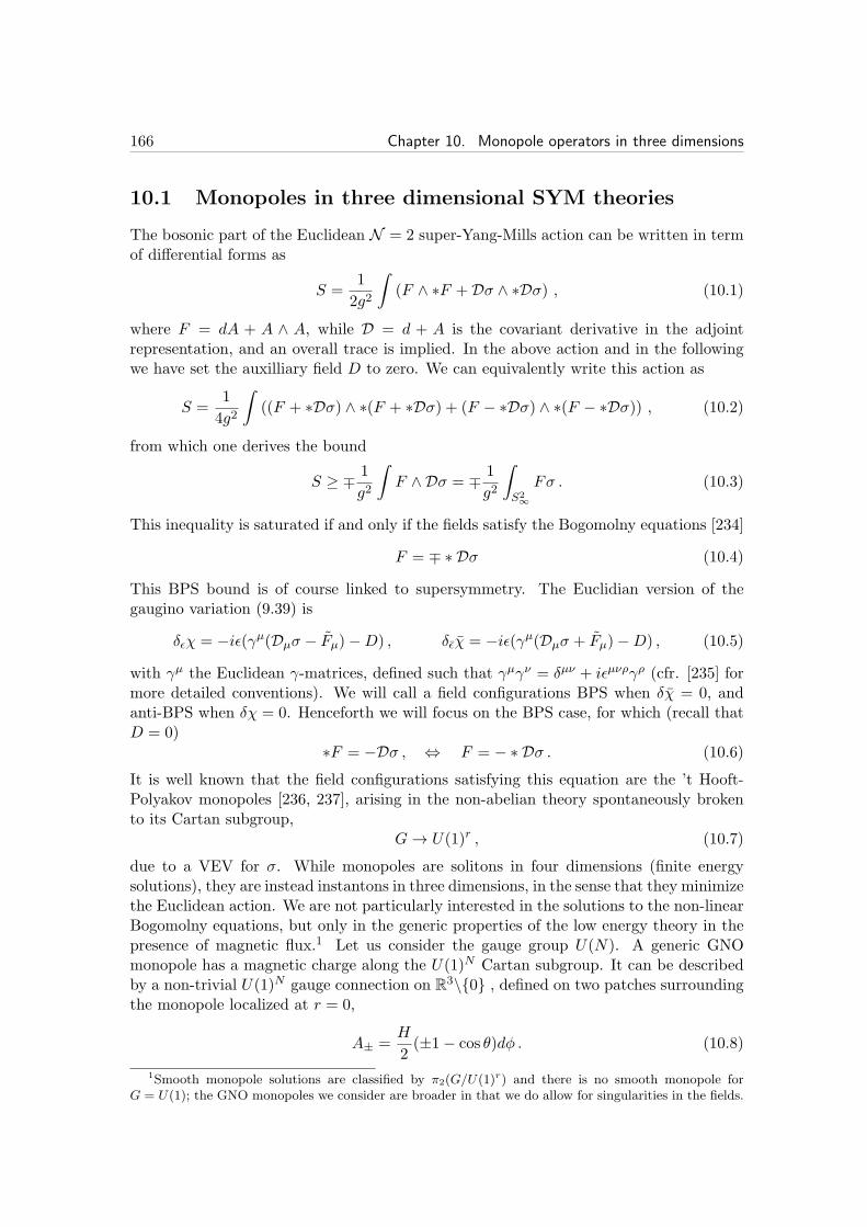
166 Chapter 10. Monopole operators in three dimensions
10.1 Monopoles in three dimensional SYM theories
The bosonic part of the Euclidean N = 2 super-Yang-Mills action can be written in termof differential forms as
S =1
2g2
∫
(F ∧ ∗F +Dσ ∧ ∗Dσ) , (10.1)
where F = dA + A ∧ A, while D = d + A is the covariant derivative in the adjointrepresentation, and an overall trace is implied. In the above action and in the followingwe have set the auxilliary field D to zero. We can equivalently write this action as
S =1
4g2
∫
((F + ∗Dσ) ∧ ∗(F + ∗Dσ) + (F − ∗Dσ) ∧ ∗(F − ∗Dσ)) , (10.2)
from which one derives the bound
S ≥ ∓ 1
g2
∫
F ∧ Dσ = ∓ 1
g2
∫
S2∞
Fσ . (10.3)
This inequality is saturated if and only if the fields satisfy the Bogomolny equations [234]
F = ∓ ∗ Dσ (10.4)
This BPS bound is of course linked to supersymmetry. The Euclidian version of thegaugino variation (9.39) is
δǫχ = −iǫ(γµ(Dµσ − Fµ)−D) , δǫχ = −iǫ(γµ(Dµσ + Fµ)−D) , (10.5)
with γµ the Euclidean γ-matrices, defined such that γµγν = δµν + iǫµνργρ (cfr. [235] formore detailed conventions). We will call a field configurations BPS when δχ = 0, andanti-BPS when δχ = 0. Henceforth we will focus on the BPS case, for which (recall thatD = 0)
∗F = −Dσ , ⇔ F = − ∗ Dσ . (10.6)
It is well known that the field configurations satisfying this equation are the ’t Hooft-Polyakov monopoles [236, 237], arising in the non-abelian theory spontaneously brokento its Cartan subgroup,
G→ U(1)r , (10.7)
due to a VEV for σ. While monopoles are solitons in four dimensions (finite energysolutions), they are instead instantons in three dimensions, in the sense that they minimizethe Euclidean action. We are not particularly interested in the solutions to the non-linearBogomolny equations, but only in the generic properties of the low energy theory in thepresence of magnetic flux.1 Let us consider the gauge group U(N). A generic GNOmonopole has a magnetic charge along the U(1)N Cartan subgroup. It can be describedby a non-trivial U(1)N gauge connection on R
3\0 , defined on two patches surroundingthe monopole localized at r = 0,
A± =H
2(±1− cos θ)dφ . (10.8)
1Smooth monopole solutions are classified by π2(G/U(1)r) and there is no smooth monopole forG = U(1); the GNO monopoles we consider are broader in that we do allow for singularities in the fields.
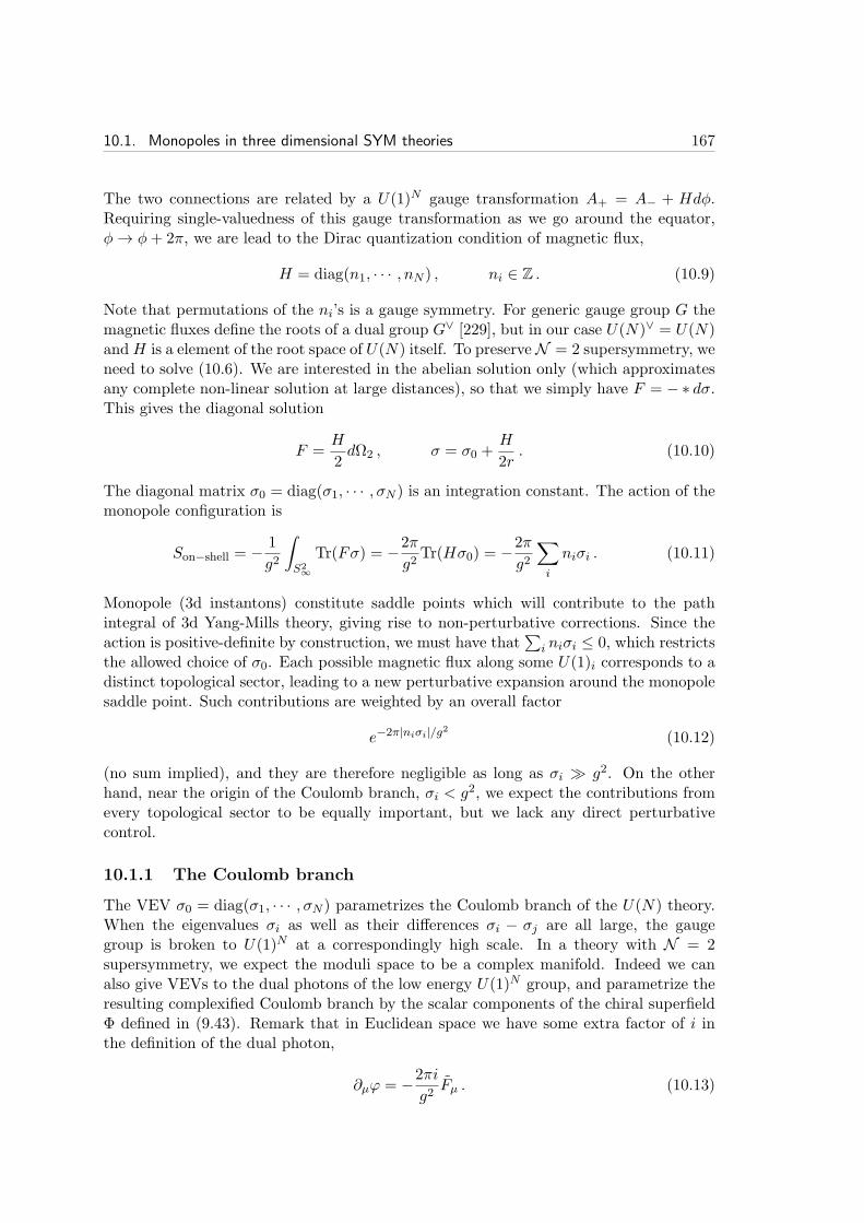
10.1. Monopoles in three dimensional SYM theories 167
The two connections are related by a U(1)N gauge transformation A+ = A− + Hdφ.Requiring single-valuedness of this gauge transformation as we go around the equator,φ→ φ+ 2π, we are lead to the Dirac quantization condition of magnetic flux,
H = diag(n1, · · · , nN ) , ni ∈ Z . (10.9)
Note that permutations of the ni’s is a gauge symmetry. For generic gauge group G themagnetic fluxes define the roots of a dual group G∨ [229], but in our case U(N)∨ = U(N)andH is a element of the root space of U(N) itself. To preserveN = 2 supersymmetry, weneed to solve (10.6). We are interested in the abelian solution only (which approximatesany complete non-linear solution at large distances), so that we simply have F = −∗ dσ.This gives the diagonal solution
F =H
2dΩ2 , σ = σ0 +
H
2r. (10.10)
The diagonal matrix σ0 = diag(σ1, · · · , σN ) is an integration constant. The action of themonopole configuration is
Son−shell = −1
g2
∫
S2∞
Tr(Fσ) = −2π
g2Tr(Hσ0) = −
2π
g2
∑
i
niσi . (10.11)
Monopole (3d instantons) constitute saddle points which will contribute to the pathintegral of 3d Yang-Mills theory, giving rise to non-perturbative corrections. Since theaction is positive-definite by construction, we must have that
∑
i niσi ≤ 0, which restrictsthe allowed choice of σ0. Each possible magnetic flux along some U(1)i corresponds to adistinct topological sector, leading to a new perturbative expansion around the monopolesaddle point. Such contributions are weighted by an overall factor
e−2π|niσi|/g2 (10.12)
(no sum implied), and they are therefore negligible as long as σi ≫ g2. On the otherhand, near the origin of the Coulomb branch, σi < g2, we expect the contributions fromevery topological sector to be equally important, but we lack any direct perturbativecontrol.
10.1.1 The Coulomb branch
The VEV σ0 = diag(σ1, · · · , σN ) parametrizes the Coulomb branch of the U(N) theory.When the eigenvalues σi as well as their differences σi − σj are all large, the gaugegroup is broken to U(1)N at a correspondingly high scale. In a theory with N = 2supersymmetry, we expect the moduli space to be a complex manifold. Indeed we canalso give VEVs to the dual photons of the low energy U(1)N group, and parametrize theresulting complexified Coulomb branch by the scalar components of the chiral superfieldΦ defined in (9.43). Remark that in Euclidean space we have some extra factor of i inthe definition of the dual photon,
∂µϕ = −2πi
g2Fµ . (10.13)
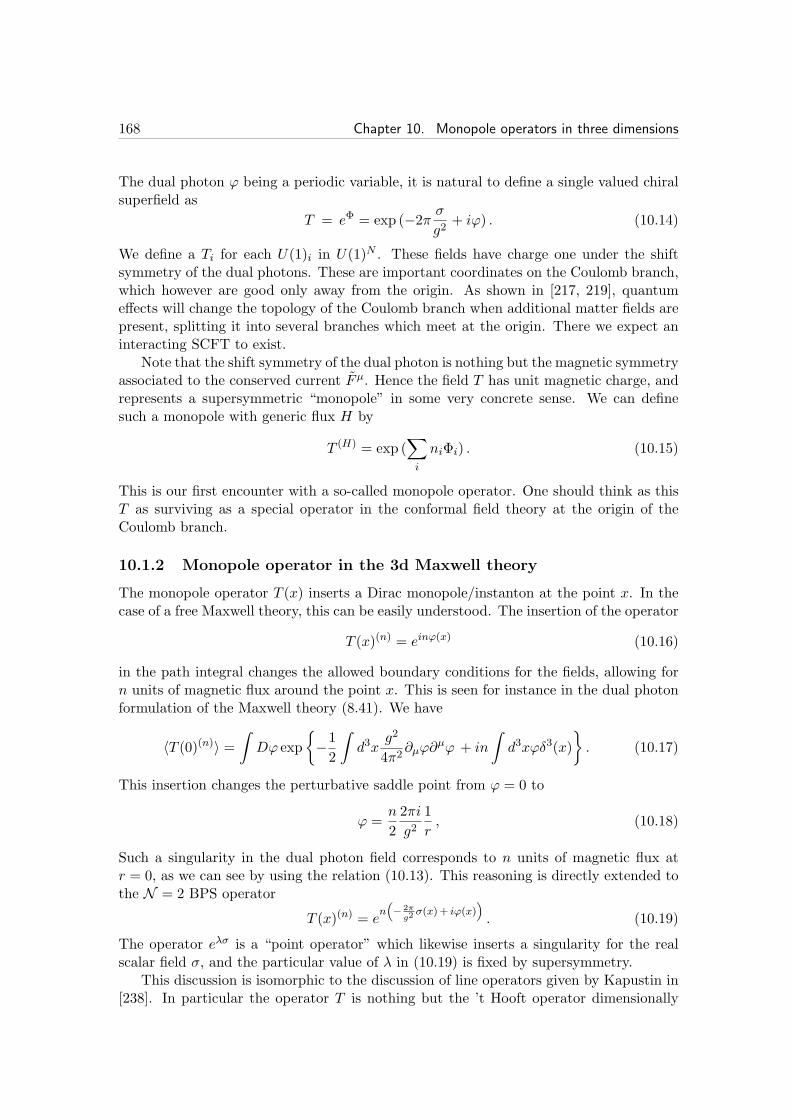
168 Chapter 10. Monopole operators in three dimensions
The dual photon ϕ being a periodic variable, it is natural to define a single valued chiralsuperfield as
T = eΦ = exp (−2π σg2
+ iϕ) . (10.14)
We define a Ti for each U(1)i in U(1)N . These fields have charge one under the shiftsymmetry of the dual photons. These are important coordinates on the Coulomb branch,which however are good only away from the origin. As shown in [217, 219], quantumeffects will change the topology of the Coulomb branch when additional matter fields arepresent, splitting it into several branches which meet at the origin. There we expect aninteracting SCFT to exist.
Note that the shift symmetry of the dual photon is nothing but the magnetic symmetryassociated to the conserved current Fµ. Hence the field T has unit magnetic charge, andrepresents a supersymmetric “monopole” in some very concrete sense. We can definesuch a monopole with generic flux H by
T (H) = exp (∑
i
niΦi) . (10.15)
This is our first encounter with a so-called monopole operator. One should think as thisT as surviving as a special operator in the conformal field theory at the origin of theCoulomb branch.
10.1.2 Monopole operator in the 3d Maxwell theory
The monopole operator T (x) inserts a Dirac monopole/instanton at the point x. In thecase of a free Maxwell theory, this can be easily understood. The insertion of the operator
T (x)(n) = einϕ(x) (10.16)
in the path integral changes the allowed boundary conditions for the fields, allowing forn units of magnetic flux around the point x. This is seen for instance in the dual photonformulation of the Maxwell theory (8.41). We have
〈T (0)(n)〉 =∫
Dϕ exp
−1
2
∫
d3xg2
4π2∂µϕ∂
µϕ + in
∫
d3xϕδ3(x)
. (10.17)
This insertion changes the perturbative saddle point from ϕ = 0 to
ϕ =n
2
2πi
g21
r, (10.18)
Such a singularity in the dual photon field corresponds to n units of magnetic flux atr = 0, as we can see by using the relation (10.13). This reasoning is directly extended tothe N = 2 BPS operator
T (x)(n) = en(
− 2πg2σ(x)+ iϕ(x)
)
. (10.19)
The operator eλσ is a “point operator” which likewise inserts a singularity for the realscalar field σ, and the particular value of λ in (10.19) is fixed by supersymmetry.
This discussion is isomorphic to the discussion of line operators given by Kapustin in[238]. In particular the operator T is nothing but the ’t Hooft operator dimensionally

10.2. Monopole operators in 3d CFT 169
reduced from four to three dimensions. This means that T stands for ’T Hooft, althoughwe will call it a “monopole operator” to conform to fashion.
Once we turn on interactions, the dual photon trick is not applicable anymore, butnevertheless the monopole operator is still a well defined concept. At least this is so inany conformal field theory, which we will now discuss.
10.2 Monopole operators in 3d CFT
In [230, 231], monopole operators where defined in 3d conformal field theories with abeliangauge fields. Consider for instance an abelian Chern-Simons theory coupled to matter. Itis classicaly conformal, and we assume for the moment that this property is not broken byquantum effects. A monopole operator, also sometimes called vortex operator, is simplyone which inserts n units of magnetic charge at a single point in R
3. This means thatthe OPE of such an operator O with the conserved current Fµ has a singularity
Fµ(x)O(y) ∼ n
2
1
|x− y|2O(y) . (10.20)
In the path integral language, such an operator inserts a new boundary condition on thegauge field, requiring that the magnetic flux around the point p = yµ be n. To have acomplete definition, we need to specify also the new boundary conditions for all the otherfields in the theory, which must now live on the punctured space R3\p. In general theremight be many allowed operators with the same magnetic charge.
A more manageable definition is obtained by using radial quantization instead of theoperator language. In the radial quantization picture a monopole operator is nothing buta state on R × S2 with n units of magnetic flux through S2. This makes also clear whylocal monopole operators are specific to three dimensions: In four dimensions there is nosuch local operators because vector bundles on S3 do not carry any interesting topologicalnumbers (4d ’t Hooft operator are extended operators corresponding to the insertion ofa monopole worldline) [238]. To go from the theory on R
3 to the theory on R × S2, wechange coordinates to τ = ln r, and we redefine all the fields as
φ = e−∆(φ)τ φ , (10.21)
where ∆(φ) is the scaling dimension of φ, and φ are the new fields we use in the radialquantization picture.
We must also discuss the issue of gauge invariance. Gauge invariance of a state onR× S2 is simply Gauss law, which can be written
δS
δAτ|ψ〉 = 0 , (10.22)
for any physical state |ψ〉 (Aτ is the τ component of the gauge field). In the case of aChern-Simons matter theory of the generic form (9.66), we have
(k
2πF τ + ρ
)
|ψ〉 = 0 , (10.23)

170 Chapter 10. Monopole operators in three dimensions
where ρ = Jτ is the charge density operator. This means that, for gauge invariance of astate carrying electric charge Q together with n units of magnetic flux, we need
kn+Q = 0 . (10.24)
In particular, monopole operator must always be “dressed” by appropriate matter fieldsin a Chern-Simons theory. Indeed, a “bare” monopole operator of magnetic charge ncorresponds to a state with an electric tadpole, since its action contains a term
S ⊃ k
4π
∫
A ∧ dA = kn
∫
A0 dt . (10.25)
This tadpole can only be cancelled by adding additional matter fields for a total charge ofQ = −kn. In the following chapters we will keep referring to the bare monopole operatorT (n) as “the” monopole operators, mainly for notational convenience. We will write gaugeinvariant operators schematically as
O(n) ∼ T (n)φ1 · · ·φkn . (10.26)
Nevertheless it should be kept in mind that only the gauge invariant operators have aphysical meaning. This is true in particular for such operators which do not have anydescription in term of Lagrangian fields, in general. We will not discuss in any detail thenon-abelian extension of these results, although they are of much interest in relation withthe AdS4/CFT3 correspondence.
10.2.1 N = 2 BPS monopole operators
Consistently with the discussion of section (10.1), N = 2 BPS monopole operators whichcreate some flux at r = 0 in R
3 must also set a boundary condition
limr→0
σ =n
2r(10.27)
for the scalar field σ in the vector supermultiplet. To discuss the corresponding statein R× S2, we need to consider the curved space version of the gaugino variation (10.5).This was studied in [235], where it is found that (setting to zero the VEV of all the otherfields)
δǫχ ∼ γµ(
Fµǫ+ (∂µσ)ǫ+ 2σ∇µǫ)
, (10.28)
where ∇ is the spin connection, and ǫ must be a Killing spinor. The solution to δǫχ = 0is more easily found by simply rescaling the solution (10.10), which gives
F =H
2dΩ2 , σ =
n
2. (10.29)
This means that the field σ must have a constant VEV n/2 at τ = −∞.

10.2. Monopole operators in 3d CFT 171
10.2.2 Induced charges from quantum effects
So far we have discussed the concept of monopole operator assuming that the CFT hasa weakly coupled Lagrangian description. For most of the models with N = 2 we willconsider this is not the case. One way to circumvent this difficulty is to work in a weaklycoupled UV completion, for instance in the UV of a YM-CS-matter theory which UVcompletes the CS-matter theory, as done in [235]. Another weakly coupled crutch isobtained by taking the CS level k to be large, or one can also take the number of flavorfields Nf to be large [230, 231].
We now discuss some quantum properties of monopole operator is such a weaklycoupled limit, for N = 2 theories. In particular, we would like to compute the exactR-charge of the bare monopole operator in the SCFT. With that knowledge we can thencompute the exact dimension of any chiral primaries monopole operator, in principle, ifwe know the R-charge of all the Lagrangian fields. Note that in general we do not knowwhich is the exact superconformal R-charge, but we can still express the correction to theR-charge of a given monopole operator in term of the unknown R-charges of the matterfields. Actually we can also compute the quantum correction to any U(1) charge Q.
The conformal dimension of the bare monopole operator is the energy of the corre-sponding state in radial quantization. This energy vanishes classically, but in the quantumtheory it is usually strongly renormalized. In the weakly coupled theory the main effectwill come from fluctuations of free quantum fields charged under a classical monopolebackground. In [230] it was shown that only the fermions contribute to this zero pointenergy, so we will discuss the fermions only.
Consider a particular U(1) gauge group (it could be part of a larger gauge group). Inthe presence of a N = 2 monopole background for this vector multiplet, any fermion ψcharged under this U(1) will satisfy the wave equation
(γµDµ ±n
2)ψ(τ, θ, φ) = 0 . (10.30)
The ± is for BPS or anti-BPS background. The first term is the Dirac operator in thismonopole background,
γµDµ = γτ∂τ +DS2 , with DS2 = γa(∇a + iAa) . (10.31)
The second term in (10.30) comes from the coupling ψσψ. The eigenvalues and eigenfunc-tions of DS2 were worked out in [239], for instance. Let J be the total angular momentumoperator, with eigenvalue j, and let n be the magnetic flux. We have
DS2Ψ0nm = 0 for j =
|n| − 1
2(10.32)
DS2Ψ±njm = i∆±
jnΨ±njm for j =
|n|+ 1
2,|n|+ 3
2, · · · (10.33)
with m = −j, · · · , j, and ∆±jn some eigenvalues which can be found e.g. in [235]. Hence
there are |n| zero modes of this Dirac operator on S2. On the other hand, the equation(10.30) has no zero energy solution: each mode Ψ±
njm corresponds to a state of energy
±|j + 12 |, while the zero modes Ψ0
nm correspond to states of energy |n|2 . This means that
the vacuum state of the bare monopole is unique. From there one can compute any charge
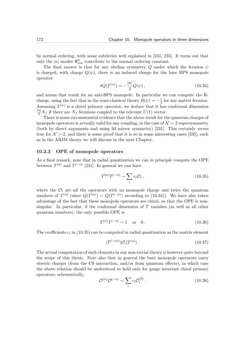
172 Chapter 10. Monopole operators in three dimensions
by normal ordering, with some subtleties well explained in [231, 235]. It turns out thatonly the |n| modes Ψ0
nm contribute to the normal ordering constant.The final answer is that for any abelian symmetry Q under which the fermion ψ
is charged, with charge Q(ψ), there is an induced charge for the bare BPS monopoleoperator
δQ(T (n)) = −|n|2Q(ψ) , (10.34)
and minus that result for an anti-BPS monopole. In particular we can compute the R-charge, using the fact that in the semi-classical theory R(ψ) = −1
2 for any matter fermion.
Assuming T (n) is a chiral primary operator, we deduce that it has conformal dimension|n|2 Nf if there are Nf fermions coupled to the relevant U(1) vector.
There is some circumstantial evidence that the above result for the quantum charges ofmonopole operators is actually valid for any coupling, in the case ofN = 2 supersymmetry(both by direct arguments and using 3d mirror symmetry) [231]. This certainly seemstrue for N > 2, and there is some proof that it is so in some interesting cases [235], suchas in the ABJM theory we will discuss in the next Chapter.
10.2.3 OPE of monopole operators
As a final remark, note that in radial quantization we can in principle compute the OPEbetween T (n) and T (−n) [231]. In general we can have
T (n)T (−n) ∼∑
i
ciOi , (10.35)
where the Oi are all the operators with no monopole charge and twice the quantumnumbers of T (n) (since Q(T (n)) = Q(T (−n)) according to (10.34)). We have also takenadvantage of the fact that these monopole operators are chiral, so that the OPE is non-singular. In particular, if the conformal dimension of T vanishes (as well as all otherquantum numbers), the only possible OPE is
T (n)T (−n) ∼ 1 or 0 . (10.36)
The coefficients ci in (10.35) can be computed in radial quantization as the matrix element
〈T (−n)†|Oi|T (n)〉 . (10.37)
The actual computation of such elements in any non-trivial theory is however quite beyondthe scope of this thesis. Note also that in general the bare monopole operators carryelectric charges (from the CS interaction, and/or from quantum effects), in which casethe above relation should be understood to hold only for gauge invariant chiral primaryoperators; schematically,
O(n)O(−n) ∼∑
i
ciO(0)i . (10.38)
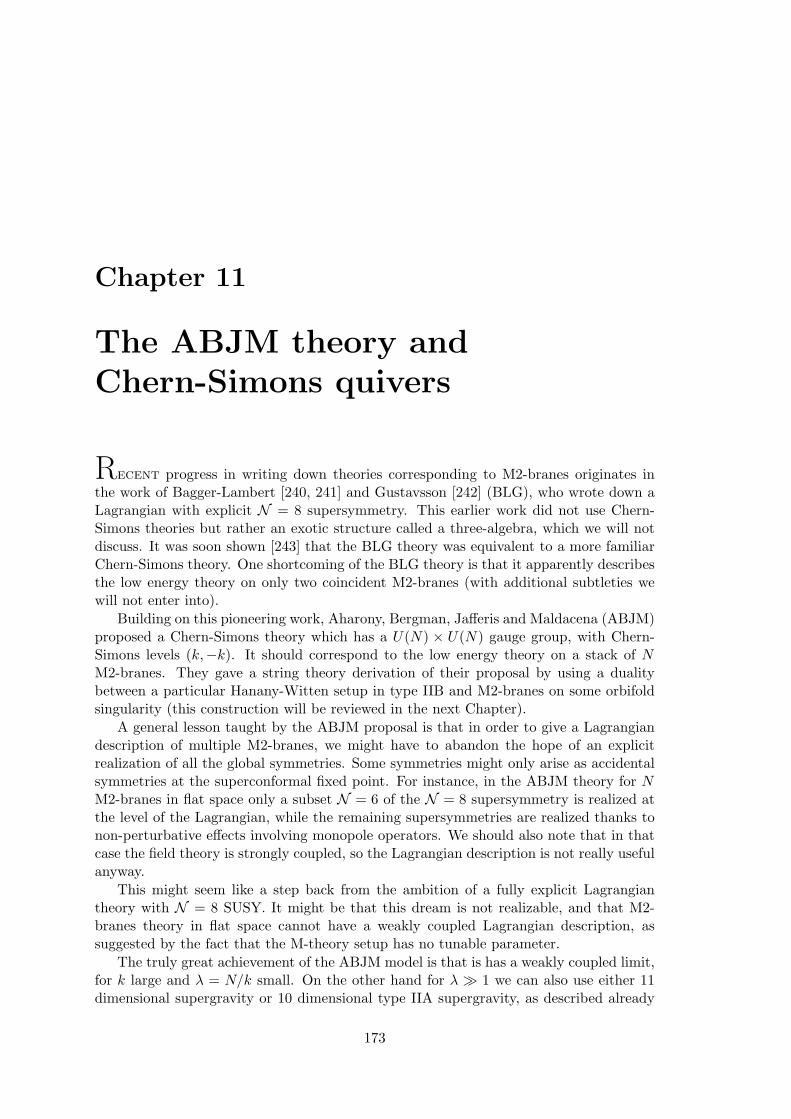
Chapter 11
The ABJM theory andChern-Simons quivers
Recent progress in writing down theories corresponding to M2-branes originates inthe work of Bagger-Lambert [240, 241] and Gustavsson [242] (BLG), who wrote down aLagrangian with explicit N = 8 supersymmetry. This earlier work did not use Chern-Simons theories but rather an exotic structure called a three-algebra, which we will notdiscuss. It was soon shown [243] that the BLG theory was equivalent to a more familiarChern-Simons theory. One shortcoming of the BLG theory is that it apparently describesthe low energy theory on only two coincident M2-branes (with additional subtleties wewill not enter into).
Building on this pioneering work, Aharony, Bergman, Jafferis and Maldacena (ABJM)proposed a Chern-Simons theory which has a U(N) × U(N) gauge group, with Chern-Simons levels (k,−k). It should correspond to the low energy theory on a stack of NM2-branes. They gave a string theory derivation of their proposal by using a dualitybetween a particular Hanany-Witten setup in type IIB and M2-branes on some orbifoldsingularity (this construction will be reviewed in the next Chapter).
A general lesson taught by the ABJM proposal is that in order to give a Lagrangiandescription of multiple M2-branes, we might have to abandon the hope of an explicitrealization of all the global symmetries. Some symmetries might only arise as accidentalsymmetries at the superconformal fixed point. For instance, in the ABJM theory for NM2-branes in flat space only a subset N = 6 of the N = 8 supersymmetry is realized atthe level of the Lagrangian, while the remaining supersymmetries are realized thanks tonon-perturbative effects involving monopole operators. We should also note that in thatcase the field theory is strongly coupled, so the Lagrangian description is not really usefulanyway.
This might seem like a step back from the ambition of a fully explicit Lagrangiantheory with N = 8 SUSY. It might be that this dream is not realizable, and that M2-branes theory in flat space cannot have a weakly coupled Lagrangian description, assuggested by the fact that the M-theory setup has no tunable parameter.
The truly great achievement of the ABJM model is that is has a weakly coupled limit,for k large and λ = N/k small. On the other hand for λ ≫ 1 we can also use either 11dimensional supergravity or 10 dimensional type IIA supergravity, as described already
173
174 Chapter 11. The ABJM theory and Chern-Simons quivers
(a) ABJM quiver. (b) Toric diagram ofC
4/Zk.
Figure 11.1: The ABJM quiver and its moduli space. The gauge group is U(N) × U(N) withChern-Simons levels (k,−k). The toric diagram of C
4/Zk contains four points, which can betaken as (1, 0, 0), (0, 1, 0), (1, 1, 0) and (0, 0, k) (here k = 3).
in Chapter 8. In that context all the heavy machinery of the AdS/CFT correspondencecan be applied fruitfully. For instance we can extrapolate results for BPS quantities fromweak to strong coupling1.
This Part of the thesis is concerned with the generalization of the ABJM constructionto instances of AdS4/CFT3 dualities with less supersymmetries. In the next chapter wewill review an interesting N = 3 construction, which directly generalizes ABJM in severaldirections. In this chapter we are particularly interested in N = 2 Chern-Simons quivertheories [244, 245]. They are candidates to describe M2-branes at Calabi-Yau fourfoldsingularities. Remark that examples with minimal N = 1 supersymmetry have also beenproposed [246, 247, 248, 249].
In the first two sections of this Chapter we review the ABJM proposal and explainthe crucial role played by monopole operators. In the remaining of the Chapter we brieflypresent some attempts in the literature towards building Chern-Simons quiver for M2-branes on any Calabi-Yau cone. We will focus on the toric case, which is more manageable2. In particular we explain a generalization of the fast forward algorithm [251, 252, 253]which will be useful in Chapter 13.
11.1 The ABJM theory
In this section we introduce the famous ABJM theory [202], which is a Chern-Simonstheory with N = 6 supersymmetry. The matter content is the same as the famousconifold quiver, as shown in Fig. 11.1(a). It is a Chern-Simons matter theory with gauge
1This assumes that we can treat λ as continuous in some regimes.2The non-toric case is of interest too, mainly because toric Calabi-Yau fourfolds do not admit complex
deformations [250]. A correspondence between a Chern-Simons quiver and a non-toric 8 dimensionalconifold was initiated in [199], where it is shown that a complex deformation of the cone corresponds toa relevant deformation of the superpotential.
11.1. The ABJM theory 175
group U(N)k×U(N)−k, where the subscripts (k,−k) are the Chern-Simons levels of eachU(N) factor. In N = 2 notation, we have four chiral matter fields (A1, A2, B1, B2), whereA1, A2 transform in the (N, N) of the gauge group, and B1, B2 in the (N ,N). Let usdenote the N = 2 vector superfields by V1 and V2, for the first and second gauge group.The ABJM Lagrangian reads
LABJM = LCS [V1; k] + LCS [V2,−k] +∫
d4θ
2∑
i=1
Tr(
−A†ieV1Aie
−V2 −B†i e
−V1BieV2)
+
∫
d2θ4π
kTr(
ǫijǫklAiBkAjBl
)
+ c.c . (11.1)
The N = 2 Chern-Simons terms LCS are given by (9.62)-(9.63). The superpotentialcoupling 4π/k is fixed by the requirement of N = 3 supersymmetry, as in Section 9.4.4.We can derive it by writing the action in term of an auxiliary complex scalar for eachvector multiplet (in which case the auxiliary fields fill a N = 4 vector multiplet, whichcontains three real scalars). Consider the superpotential
W = − k
8πTr(Φ2
1 − Φ22) +
∑
i
Tr(BiΦ1Ai +AiΦ2Bi) (11.2)
where the coupling between the N = 4 hypermultiplets Hi = (Ai, Bi) and the scalarsfrom the vector multiplets is fixed by supersymmetry, while the Chern-Simons mass termfor Φ1 and Φ2 breaks N = 4 to N = 3. Integrating out these fields, we obtain
W =4π
kTr(A1B1A2B2 −A1B2A2B1) . (11.3)
One can check that it can be written as in (11.1), which makes explicit that the theorypreserves a larger SU(2)A×SU(2)B flavor symmetry, under which (A1, A2) and (B1, B2)transform independently. In addition, the theory has a SU(2)R R-symmetry, under which
(A1, B†1) and (A2, B
†2) are doublets. In the N = 2 notations we only see explicitly the
Abelian subgroup U(1)R, under which all chiral superfields have charge 12 . The SU(2)R
does not commute with the SU(2)A×SU(2)B flavor symmetry. It is easy to see that thethree SU(2) factors generate a larger SU(4)R R-symmetry, under which the fields
(C1, C2, C3, C4) = (A1, A2, B†1, B
†2) (11.4)
transform in the fundamental representation. Since this SU(4) ∼= Spin(6) is a R-symmetry, this is the first hint that the ABJM action in fact preserves N = 6 super-symmetry. By integrating out all the auxiliary fields and writing the Lagrangian in itsfull glory, in term of component fields, one can check that the action is indeed invariantunder this SU(4)R [202, 214]. The full global symmetry of the ABJM model is
SU(4)R × U(1)b , (11.5)
where the so-called baryonic symmetry U(1)b is the symmetry which assigns charge +1to Ai and −1 to Bi.
The proposal of ABJM is that this Chern-Simons SCFT is dual to M-theory onAdS4 × S7/Zk, for a particular Zk quotient which we will discuss momentarily. At large

176 Chapter 11. The ABJM theory and Chern-Simons quivers
k the theory is weakly coupled if the ’t Hooft coupling λ = N/k is small, while for λ largewe can use either M-theory or type IIA string theory, as described in Chapter 8, section8.2.
This duality is very interesting because of the large amount of supersymmetry pre-served. In the last two years a great deal of work has lent credence to this proposal. Ba-sically any of the checks that could be done in the case of the duality between AdS5×S5
and N = 4 SYM has some analog in the ABJM context, and much of it has been donealready.
11.1.1 The ABJM moduli space
Let us compute the moduli space of the ABJM theory. Consider first the Abelian case.The gauge group is U(1)k ×U(1)−k. Integrating out the auxiliary fields D1, D2 fixes thevalue of σ1, σ2 to
σ1 = σ2 =2π
k
∑
i
(|Ai|2 − |Bi|2
). (11.6)
Since W = 0 in the Abelian case, we have the four variables Ai, Bi, which remainunconstrained3. We still have to take care of gauge invariance, however. Naively we wouldhave to impose the U(1)1 − U(1)2 gauge symmetry, which is the only one which couplesto the matter fields. However this would not give a Kahler moduli space (because due tothe CS terms there is no associated moment map to make a proper Kahler quotient). Amore careful consideration of the CS interactions give the resolution of this puzzle. Letus define
AD = A1 +A2 , Ab = A1 −A2 . (11.7)
The Abelian Chern-Simons term is then written
SCS =k
4π
∫
Ab ∧ dAD , (11.8)
Only Ab couples to the matter fields, while AD only appears here, in that combination.We can then use the dual photon trick, writing the action in term of FD = dAD andimposing the Bianchi identity through a Lagrange multiplier ϕ
SCS =k
4π
∫
Ab ∧ FD +1
2π
∫
ϕ ∧ dFD . (11.9)
Integrating out FD, we see that the dual photon is related to the gauge field Ab, as
Ab =2
kdϕ , (11.10)
so we can trade one for the other, and ϕ is not gauge invariant. Although it is invariantunder U(1)D, under a U(1)b gauge transformation Ab → Ab + dΛ we have
ϕ→ ϕ+k
2Λ . (11.11)
3The reader should contrast this with the situation in the N = 1 conifold theory, where we have aD-term constraint |Ai|2 − |Bi|2 = 0. Here the “D-term” can be arbitrary, and its value only determinesthe value of the auxiliary fields σ1, σ2.

11.2. Chiral ring and monopole operators 177
Flux quantization implies that ϕ has period π (see below around equ. (11.41) for adiscussion in the general case of N = 2 CS quivers). If we gauge fix ϕ = 0, we still havea residual Zk gauge symmetry, Λ = 2πn/k, n ∈ Z, which acts on the matter fields as
(Ai, Bi) → (e2πink Ai, e
−2πink Bi) . (11.12)
Let us summarize the logic of this computation. The naive thing to do would be toquotient by U(1)b from the start, but this would not give a complex moduli space. Theresolution of this puzzle is that we can dualize the photon of U(1)D, giving us an extrareal moduli. We then need to quotient by U(1)b, but the dual photon ϕ transforms underthe gauge symmetry U(1)b. It is convenient to get rid of ϕ by gauge fixing it to zero,which however leaves a discrete Zk gauge symmetry. We then have the moduli spaceC4/Zk, with Zk acting on
(z1, z2, z3, z4) → (ωz1, ωz2, ω−1z3, ω
−1z4) , ω = e2πink . (11.13)
We could also choose a different complex structure, for instance the one of (11.4), whichmakes the SU(4)R and the associated N = 6 SUSY more manifest. We prefer to focuson the description in term of the complex structure (11.13) since it is the one inducedby the particular N = 2 notation we chose, and we are interested in generalizing thediscussion to arbitrary N = 2 Chern-Simons quivers. Note that C4/Zk is toric, with thetoric diagram given in Figure 11.1(b).
The non-Abelian generalization is straightforward in this case, because we can diag-onalize all the matrices involved (due to the F-term relations). As expected, the modulispace of the U(N)× U(N) theory corresponds to the moduli space of N M2-branes at aC4/Zk singularity,
M = SymN(C4/Zk
). (11.14)
11.2 Chiral ring and monopole operators
An important check of this AdS/CFT duality proposal is whether the chiral ring of thelarge N theory matches the supergravity spectrum. Consider first the Abelian case,N = 1, and focus on N = 2 chiral fields for simplicity. If we only consider the fieldsappearing in the Lagrangian, the gauge invariant operators are of the form AiBj , whichgives an algebraic description of the conifold, of complex dimension 3, instead of theorbifold C
4/Zk. The chiral ring also contains monopole operators, which makes thestudy of chiral rings a much more complicated problem than in 4d SCFT, where theclassical and quantum chiral rings are isomorphic. We can have either so-called diagonalor off-diagonal fluxes along U(1)k×U(1)−k. A bare monopole operator with off-diagonalfluxes (n,−n) would have an electric charge (kn, kn). Such an operator cannot be madeinvariant using the field content of the theory, hence it cannot appear in the spectrum.Another way to see this is that Gauss law for AD in (11.8) would read
∫
S2
Fb = 0 (11.15)
for any state on R × S2. Hence we only have to consider the diagonal operator T (n),which has magnetic flux (n, n) along U(1)k × U(1)−k. It has electric charge (nk,−nk),
178 Chapter 11. The ABJM theory and Chern-Simons quivers
according to the discussion of the previous Chapter. It can be shown that the conformaldimension of this bare monopole operator is precisely zero [214]. We can write chiraloperators of the form (take n ≥ 0)
O(n) ∼ T (n)Bkn(AB)l , O(−n) ∼ T (−n)Akn(AB)l , (11.16)
of conformal dimension 12kn+ l. Recall that this way of writing the monopole operators
is mainly a notational convenience. Their proper definition is through the correspondingstate in R× S2. It can be checked that the basic monopole operators
O(−1)i1···ik
= T (−1)Ai1 · · ·Aik , O(1)i1···ik
= T (1)Bi1 · · ·Bik , (11.17)
generate the full chiral ring
C[O(−1)i1···ik
,O(1)i1···ik
] ∼= Spec(C4/Zk
). (11.18)
Monopole operators correspond to states which have momentum n/R along the M-theorycircle (D0-branes in type IIA). The isometry U(1)M associated to the M-theory fibrationcorresponds to the conserved current ∗FD in the ABJM theory. Indeed, we have
k
4π∗ FD = Jb , (11.19)
where Jb is the current of the baryonic symmetry U(1)b. The isometry U(1)M ∼= U(1)bcorresponds to a shift of the dual photon ϕ or equivalently to a rotation of the phase ofthe bifundamental fields. This global symmetry is to be distinguished from the gaugesymmetry which corresponds to a simultaneous shift of the dual photon and of the phaseof the bifundamental fields.
11.2.1 Non-Abelian case
In the non-Abelian case, a generic diagonal monopole has fluxes H = (n1, · · · , nN ), andH lies in the root lattice of the diagonal U(N). The space dual to the root lattice is theweight lattice. Any vector in the weight lattice of U(N), W = (e1, · · · , eN ), determinesa corresponding representation of highest weights given by W [254, 255]. Consider anordering of W with e1 ≥ e2 ≥ · · · ≥ eN . Then, the corresponding Young tableau has e1boxes on the first row, e2 boxes on the second row, etc. It is a result of [254] that in aU(N) theory with CS level k, the monopoles H transform in the U(N) representation
W = kH = (kn1, · · · , knN ). (11.20)
It was shown in [235] that all of these bare monopole operators have vanishing R-charge atthe quantum level. Of particular interest are the monopoles with flux H = (n, 0, · · · , 0),which transforms in the kn-symmetric product of the fundamental representation. Thegauge invariant operators one can build from this particular T (n) are the analog of (11.16).They should be chiral primary operators, corresponding to a chiral ring isomorphic to
Spec(C4/Zk
), (11.21)
11.3. N = 2 Abelian quivers and their classical moduli space 179
and they should match to the supergravity excitations along AdS4 × S7/Zk. On theother hand, all the other possible monopole operators do not have the right symmetriesto be matched to supergravity states. Hence we expect that they are not BPS and thatthey acquire large anomalous dimensions. Anomalous dimensions of operators with nomagnetic charge can be computed in the large k limit, for instance in [256], matchingexpectations. But it is not clear (to the best of my knowledge) whether it is possible todo similar perturbative computations in the presence of monopole operators. If we workin the large k limit, monopole operators decouple from the spectrum, while in the gravitydual we can consider type IIA string theory on AdS4 × CP3. It is in this context thatmost direct checks of the ABJM proposal have been performed.
The punchline is that monopole operators are precisely very important if one wouldlike to understand the M-theory limit rather than the type IIA limit.
11.2.2 Enhanced SUSY
In the ABJM theory, the monopole operator have one additional virtue. They enhancethe supersymmetry from N = 6 to N = 8 when k = 1, 2. Indeed, C
4 and C4/Z2
both preserve a larger SO(8)R symmetry, and the corresponding N = 8 SUSY, butsuch enhanced supersymmetry is not seen in the Lagrangian. It was shown explicitly in[235, 257] how this enhancement comes about. There are 16 conserved currents associatedto the SU(4)R × U(1)b symmetry, which take the form
jµIJ = i(
CIDµC†J − (DµCI)C
†J + fermions
)
, (11.22)
where the CI ’s are as defined in (11.4). The traceless part give the currents of SU(4)R,while the trace
∑
I jII corresponds to U(1)b. When k = 1, 2, we can write down 12additional gauge invariant currents, by using monopole operators with H = (n, · · · , 0):
T (−n) i (CIDµCJ − CJDµCI + fermions) , (11.23)
written here as 6 complex currents, and n = 1, 2 for k = 2, 1, respectively. In total wehave 28 conserved currents, which generate a full SO(8)R symmetry [235]. The explicitform of the on-shell N = 8 SUSY transformations were written down in [257].
11.3 N = 2 Abelian quivers and their classical moduli space
The ABJM theory has the structure of a quiver. At first sight this is somewhat unex-pected. As we saw in Chapter 3 quivers are tightly linked with D-branes at Calabi-Yauthreefold singularities. We will see in the next Chapter that this is the case here too; forinstance the fact that the ABJM quiver is the conifold quiver is not a coincidence [258].One of the themes of this second Part of the thesis is to understand this relationshipbetter.
In this section we review the constructions of N = 2 Chern-Simons quivers initiated in[244, 245], followed by a large number of works [251, 252, 253, 259, 260, 261, 262, 263, 258,264, 199, 265, 266, 267]. The rules of the game are to work out the moduli space of anysuch Chern-Simons quiver and to check whether it can correspond to M2-branes on a CYfourfold. In the toric case we can use brane tiling methods, and an interesting algoritm

180 Chapter 11. The ABJM theory and Chern-Simons quivers
has been developed to compute the relevant branch of the moduli space [251, 252, 253],directly generalizing the forward algorithm reviewed in section 3.5.
A Chern-Simons quiver theory is a quiver in which each node correspond to a 3dvector multiplet with U(N) gauge group, and with Chern-Simons interactions only (noYang-Mills term). The Chern-Simons level of the gauge group U(N)i is written ki, andit is a quantized integer. Apart from that the quiver has the same structure as the oneswe use for D-branes: there are matter fields in bifundamental and adjoint representationsonly, and a superpotential. We restrict to quivers with gauge group
U(N)1 × U(N)2 × · · · × U(N)G . (11.24)
Different ranks for the gauge groups are possible and this is linked with either fractionalM2-branes [268] or cascading solutions [269, 270]; we will not discuss such developments4.
From now on we will focus on the Abelian case. Consider a quiver with gauge groupU(1)G and CS levels (k1, · · · , kG). The matter fields are denoted either by Xα, α =1, · · · ,M or by Xij when we want to emphasize that the field X goes from node i to nodej; we also denote i = h(α) and j = t(α) for the node at the head or tail of the arrowX. The definition of the theory also includes some superpotential W (X). It should be ofclassical dimension 2 if we want to have a weakly coupled description at large CS levels,but in general we can consider W some arbitrary polynomial in the fields, in the hopethat the theory flows to a strongly coupled fixed point for any CS levels. The Lagrangianreads
L =∑
i
LCS [Vi; ki] +∑
α
∫
d4θ(
−X†αeVt(α)Xαe
−Vh(α))
+
∫
d2θW (X) + c.c. (11.25)
The scalar superpotential isV = VF + VD , (11.26)
with the F-term part familiar from N = 1 theories in 4d,
VF =∑
α
∣∣∣∣
∂W
∂Xα
∣∣∣∣
2
(11.27)
and
VD = −∑
i
ki2πσiDi +
∑
α
|Xα|2(Dt(a) −Dh(a)) +∑
α
|Xα|2(σt(α) − σh(α))2 (11.28)
Let us define the quantity,
Di =∑
i|t(α)=i
|Xα|2 −∑
j|h(α)=j
|Xα|2 =∑
α
gi[Xα] |Xα|2 , (11.29)
which in four dimensions would be the N = 1 D-term for the gauge group U(1)i (heregi[Xα] is the electric charge of Xα under U(1)i, which is ±1 or 0 in our quivers). Inte-grating out the fields Di, we have a simple scalar potential
VD =∑
α
|Xα|2(σt(α) − σh(α))2 , (11.30)
4In the non-toric case we also expect that some theories describing “regular” M2-branes can havegauge groups with different ranks, similarly to the case of D-branes on non-toric CY threefolds.
11.3. N = 2 Abelian quivers and their classical moduli space 181
together with a set of constraintski2πσi = Di , (11.31)
which imply∑
i kiσi = 0. To compute the moduli space of such a quiver, we imposethe conditions VF = 0 and VD = 0. The F-flatness conditions ∂W/∂Xa = 0 define analgebraic variety (sometimes called the master space)
Z = Xα | dW = 0 ⊂ CM , (11.32)
like for a quiver theory in 3+1 dimensions. In addition we need to solve VD = 0 and theconstraints (11.31). We are interested in the branch of the moduli space for which
σ1 = · · · = σG ≡ σ , (11.33)
in which case VD automatically vanishes. Such a branch exists only if
∑
iki = 0 . (11.34)
This later condition will be part of our definition of a Chern-Simons quiver, because itis necessary in order to have a Calabi-Yau fourfold 5 [244], for this particular branch ofthe moduli space. The case
∑
i ki 6= 0 is associated to a non-zero Romans mass in thetype IIA gravity dual [247], a situation we will not consider. On the branch (11.33), σ isdetermined by the quantities Di,
σ
2π=∑
i
ki|k|2 Di . (11.35)
The constraints (11.31) reduce to G− 2 constraints
∑
iviDi = 0 ∀ vi such that
∑
iviki = 0 . (11.36)
In other words, in contrast to quivers in 3+1 dimensions, we only impose G − 2 D-flatness conditions, corresponding to the subgroup of U(1)G orthogonal to both
∑
i U(1)iand
∑
i kiU(1)i. The moduli space is then a Kahler quotient Z//U(1)G−2. However wemust be careful with our gauge fixing. Let us define the photons
AD =G∑
i=1
Ai , Ab =1
q
G∑
i=1
kiAi (11.37)
where q = gcdki. One can show that the only way AD enters the action is through aterm [244]
q
2πG
∫
Ab ∧ dAD . (11.38)
Dualizing AD, we have
dϕ =q
GAb , (11.39)
5For a non-toric quiver with different ranks Ni the condition to have a CY4 is∑
i kiNi = 0.
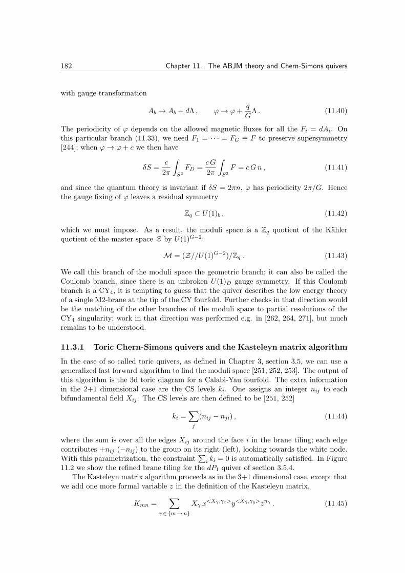
182 Chapter 11. The ABJM theory and Chern-Simons quivers
with gauge transformation
Ab → Ab + dΛ , ϕ→ ϕ+q
GΛ . (11.40)
The periodicity of ϕ depends on the allowed magnetic fluxes for all the Fi = dAi. Onthis particular branch (11.33), we need F1 = · · · = FG ≡ F to preserve supersymmetry[244]; when ϕ→ ϕ+ c we then have
δS =c
2π
∫
S2
FD =cG
2π
∫
S2
F = cGn , (11.41)
and since the quantum theory is invariant if δS = 2πn, ϕ has periodicity 2π/G. Hencethe gauge fixing of ϕ leaves a residual symmetry
Zq ⊂ U(1)b , (11.42)
which we must impose. As a result, the moduli space is a Zq quotient of the Kahlerquotient of the master space Z by U(1)G−2:
M = (Z//U(1)G−2)/Zq . (11.43)
We call this branch of the moduli space the geometric branch; it can also be called theCoulomb branch, since there is an unbroken U(1)D gauge symmetry. If this Coulombbranch is a CY4, it is tempting to guess that the quiver describes the low energy theoryof a single M2-brane at the tip of the CY fourfold. Further checks in that direction wouldbe the matching of the other branches of the moduli space to partial resolutions of theCY4 singularity; work in that direction was performed e.g. in [262, 264, 271], but muchremains to be understood.
11.3.1 Toric Chern-Simons quivers and the Kasteleyn matrix algorithm
In the case of so called toric quivers, as defined in Chapter 3, section 3.5, we can use ageneralized fast forward algorithm to find the moduli space [251, 252, 253]. The output ofthis algorithm is the 3d toric diagram for a Calabi-Yau fourfold. The extra informationin the 2+1 dimensional case are the CS levels ki. One assigns an integer nij to eachbifundamental field Xij . The CS levels are then defined to be [251, 252]
ki =∑
j
(nij − nji) , (11.44)
where the sum is over all the edges Xij around the face i in the brane tiling; each edgecontributes +nij (−nij) to the group on its right (left), looking towards the white node.With this parametrization, the constraint
∑
i ki = 0 is automatically satisfied. In Figure11.2 we show the refined brane tiling for the dP1 quiver of section 3.5.4.
The Kasteleyn matrix algorithm proceeds as in the 3+1 dimensional case, except thatwe add one more formal variable z in the definition of the Kasteleyn matrix,
Kmn =∑
γ ∈m→n
Xγ x<Xγ ,γx>y<Xγ ,γy>znγ . (11.45)

11.3. N = 2 Abelian quivers and their classical moduli space 183
Figure 11.2: Brane tiling for the dP1 quiver, refined with weights nα. The corresponding Chern-Simons quiver has CS levels (k1, k2, k3,−k1 − k2 − k3).
Computing the permanent, we have6
permK =∑
ktk x
hx(k)yhy(k)zhz(k) . (11.46)
The slopes hx, hy are defined as in (3.43), while hz is
hz(tk) =∑
α
Mkαnα . (11.47)
We easily see that the points(hx, hy, hz) ∈ Z
3 (11.48)
describe the toric diagram of the CY4 (the geometric branch) of the last section. Simply,we have that (in the notation of section 3.5)
∑
k(QF )
lkhz(k) = 0 ,
∑
k(GD)
ikhz(k) =
∑
αQiαnα = ki . (11.49)
The first relation follows from (11.47) and (3.33), while the second follows from (11.47),(3.32) and the definition of the weights nα for the fields Xα. It means that we only imposea U(1)G−2 subgroup of the quiver gauge symmetry, corresponding to the electric chargesorthogonal to U(1)b (and U(1)D).
For our dP1 example, the improved permK is
permK = X31X141X
241 +X2
12X223X
241 x+X1
12X212X
141 x
−1y+
+X112X
212X
312 z
k1 +X312X24X31 y
−1zk1 +X123X
223X24 z
k1+k2 +
+X24X31X34 zk1+k2+k3 +X1
12X212X34 yz
k1+k2+k3 .
(11.50)
Notice that setting z = 1 we reproduce the 3+1 dimensional algorithm. Thus the projec-tion of the 3d toric diagram of the 2+1 dimensional theory on the plane hz = 0 is the 2dtoric diagram of the 3+1 dimensional theory.
6Note that we change notation with respect to Chapter 3: from now on we will denote the perfectmatching variables by tk instead of pk.

184 Chapter 11. The ABJM theory and Chern-Simons quivers
If q = gcdki > 1, some internal points are not represented by any perfect matching,and the result of the GLSM has to be quotiented by Zq. Alternatively we can includeall points of the toric diagram in the GLSM, at the price of adding new fields and gaugesymmetries.
According to (11.49), the coordinates hz determine the particular U(1)b ⊂ U(1)G,whose photon Ab is related to the dual photon ϕ of the diagonal gauge group. As wediscussed already in the ABJM case (and we will come back to the point at length inChapter 13), this U(1)b corresponds to the M-theory circle in the geometric setup.
11.4 A look at proposals for M2-brane theories
In the discussion of the previous section, we did not assume that the CS quiver had awell defined “parent quiver” in 3+1 dimension. In 3+1 dimensions, there are variousconsistency conditions that a quiver has to satisfy in order to describe D3-branes at asingularity, see e.g. [72]. One such condition is cancellation of gauge anomalies, whichrestricts the allowed matter content. Another condition is that the quiver theory shouldflow to a superconformal fixed point in the IR; basically this restrict the field content sothat the number of color and flavor in each node is in the Seiberg conformal window (seeAppendix C). In 2+1 dimensions, none of these restrictions are necessary: there is nocontinuous anomaly and almost any matter content is believed to lead to a SCFT in theinfrared.
In the absence of a clear understanding of the link between M2-branes and quivers,this lead to the study of many proposals for M2-brane theories [244, 245, 251, 252, 253,259, 260, 261, 262, 263, 258, 264, 199, 265, 266, 267, 272]. The main tool to constructsuch theories is that their moduli space reproduces the expected CY4 geometry, and thatone can understand the partial resolution from one singularity to another one as Higgsingin the quiver, much like in 3+1 dimensions [262, 264, 271].
It is fair to say that most of the studies of such quivers in the litterature consider thegauge theory at the classical level only. This often implies taking a large k (CS levels)limit, even though in general the anomalous dimensions are large and there really doesnot exist any weak coupling limit.
11.4.1 Brane tilings with multiple bounds
Of particular interest to us is a new kind of brane tiling which is not obviously inconsistentin 2+1 dimensions: the so-called mutiple bounds brane tilings. These are tilings in whicha white and a black node are connected by two or more edges (an example with doublebounds is shown in Figure 11.3(a)).
The associated quiver has gauge groups with only one arrow entering and one arrowleaving; in 3+1 dimensions this corresponds to N = 1 SQCD with Nf = Nc, whichis certainly not conformal, and this is why such tilings never appear when consideringD3-branes at CY3 singularities.
A particular property of such tilings is that there are several perfect matchings whichhave the same slopes (hx, hy), but different values of hz. Indeed, consider a tiling withno multiple bound, and choose some edge X, which is contained in some number ofperfect matchings tX. We obtain a n-tuple bound tiling simply by replacing this edge
11.4. A look at proposals for M2-brane theories 185
(a) Quiver. (b) 3d Toric diagram fork = 1.
(c) Brane tiling.
Figure 11.3: Brane tiling, quiver and toric diagram of the Q1,1,1 model of [259]. Notice the twodouble-bounds in the brane tiling. The superpotential is W = −ǫijA1C1BiC2A2Bj .
X by n edges C1, · · · , Cn. For any perfect matching pX of the single bound quiver thereare n perfect matchings in this new tiling. For a generic assignment of the weights nαto the new edges Cα, we have n − 1 new points in the toric diagram, with coordinates(hx, hy, hz), but with the particular property that they all project to the same point(hx, hy) when z = 0. This means that in general the toric diagram contains a line of h+1external points (where h depends on the choice of nα). This corresponds to a complexcodimension 2 singularity, which is locally C
2×C2/Zh. A difficulty with the intepretationof the multiple bound theories as M2-brane theories is that they do not seem to accountfor such a non-isolated singularity: there are extra modes with SU(h) gauge symmetrylocalized at the singularity in M-theory (or h D6-branes in a type IIA reduction), whichare not seen in the field theory.
In Chapter 13 we will present an alternate description of the same geometries withcodimension 2 singularities. It might be that the multiple bound theories are somewhatdual to the theories of Chapter 13. Another possibility is that the multiple boundstheories are actually inconsistent (they do not describe M2-branes).
Example: a double-bound tiling for Q1,1,1.
An interesting example is the CS quiver proposed in [259] as a candidate for thedescription of M2-branes on the C(Q1,1,1) singularity. This CS quiver theory was furtherstudied in [262, 273]. The Sasaski-Einstein seven manifold Q1,1,1 is a homogenous space(SU(2) × SU(2) × SU(2))/U(1)2, and it can also be seen as a regular circle fibrationof CP1 × CP1 × CP1. For these reasons it is a nice space to study, much like the fivedimensional T 1,1 in type IIB.
The brane tiling is shown in Figure 11.3(a). It can be obtained from the conifoldtiling by doubling both edges A1 and A2 (compare to Figure 3.3(b) in Chapter 3), as
A1 → A1, C1 , A2 → C2, A2 . (11.51)
The quiver is the one of Figure 11.3(c), with CS levels (k, k,−k,−k) and sextic superpo-tential
W = A1C1B2C2A2B1 −A1C1B1C2A2B2 . (11.52)
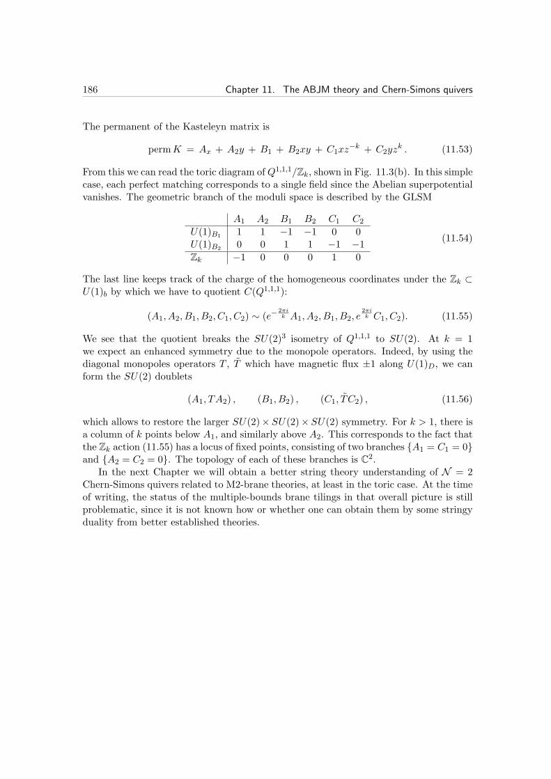
186 Chapter 11. The ABJM theory and Chern-Simons quivers
The permanent of the Kasteleyn matrix is
permK = Ax + A2y + B1 + B2xy + C1xz−k + C2yz
k . (11.53)
From this we can read the toric diagram ofQ1,1,1/Zk, shown in Fig. 11.3(b). In this simplecase, each perfect matching corresponds to a single field since the Abelian superpotentialvanishes. The geometric branch of the moduli space is described by the GLSM
A1 A2 B1 B2 C1 C2
U(1)B1 1 1 −1 −1 0 0U(1)B2 0 0 1 1 −1 −1Zk −1 0 0 0 1 0
(11.54)
The last line keeps track of the charge of the homogeneous coordinates under the Zk ⊂U(1)b by which we have to quotient C(Q1,1,1):
(A1, A2, B1, B2, C1, C2) ∼ (e−2πik A1, A2, B1, B2, e
2πik C1, C2). (11.55)
We see that the quotient breaks the SU(2)3 isometry of Q1,1,1 to SU(2). At k = 1we expect an enhanced symmetry due to the monopole operators. Indeed, by using thediagonal monopoles operators T , T which have magnetic flux ±1 along U(1)D, we canform the SU(2) doublets
(A1, TA2) , (B1, B2) , (C1, TC2) , (11.56)
which allows to restore the larger SU(2)× SU(2)× SU(2) symmetry. For k > 1, there isa column of k points below A1, and similarly above A2. This corresponds to the fact thatthe Zk action (11.55) has a locus of fixed points, consisting of two branches A1 = C1 = 0and A2 = C2 = 0. The topology of each of these branches is C2.
In the next Chapter we will obtain a better string theory understanding of N = 2Chern-Simons quivers related to M2-brane theories, at least in the toric case. At the timeof writing, the status of the multiple-bounds brane tilings in that overall picture is stillproblematic, since it is not known how or whether one can obtain them by some stringyduality from better established theories.

Chapter 12
Chern-Simons quivers fromstringy dualities
Given the construction of Chern-Simons quivers reviewed in the last chapter, it isnatural to wonder why does the quiver structure appear at all. After all, quivers areuseful tools to describe D-branes, but it is not a priori clear that M2-branes shouldbehave similarly. For instance, it is known that M2-branes theories do not behave like D-brane theories upon orbifolding [214, 274]: the Douglas-Moore [39] orbifolding procedure(see Chapter 3) on a M2-brane quiver for a space X does not lead to a quiver for M2-branes on X/Γ.
In this Chapter we explain the present understanding of the relation between M2-branes and quivers. This understanding is always through some string theory duality.In the first section we explain how the ABJM theory and some N = 3 supersymmetricgeneralizations can be obtained from a type IIB brane setup. In the second section, weexplain an interesting generalization of the ABJM quiver which naturally arises fromthis type IIB understanding: we consider adding flavors (fields in the fundamental/anti-fundamental representation) to the ABJM quiver. This prepares the ground for theunderstanding of the next Chapter.
In the last section we will consider a different understanding of Chern-Simons quiver,which comes about through the type IIA/M-theory duality. Part of that section is basedon our paper [3], written in collaboration with Stefano Cremonesi and Francesco Benini.
12.1 Fivebrane systems, M-theory/type IIB duality and
ABJM
In the original paper [202] the relation between the CS quiver theory and M2-branes onC4/Zk was given a nice string theory derivation through an interesting Hanany-Witten
setup in type IIB. This brane setup engineers a YM-CS-matter theory which flows to theCS-matter ABJM theory in the IR.
Consider type IIB string theory. Take two NS5-branes on a circle with coordinate x6
and N D3-branes wrapping this circle. Let us put the NS5-brane at x6 = 0 and the NS5’at x6 = πR6 (assuming x6 ∼ x6 +2πR6). This is T-dual to D2-branes on C×C
2/Z2×R
187
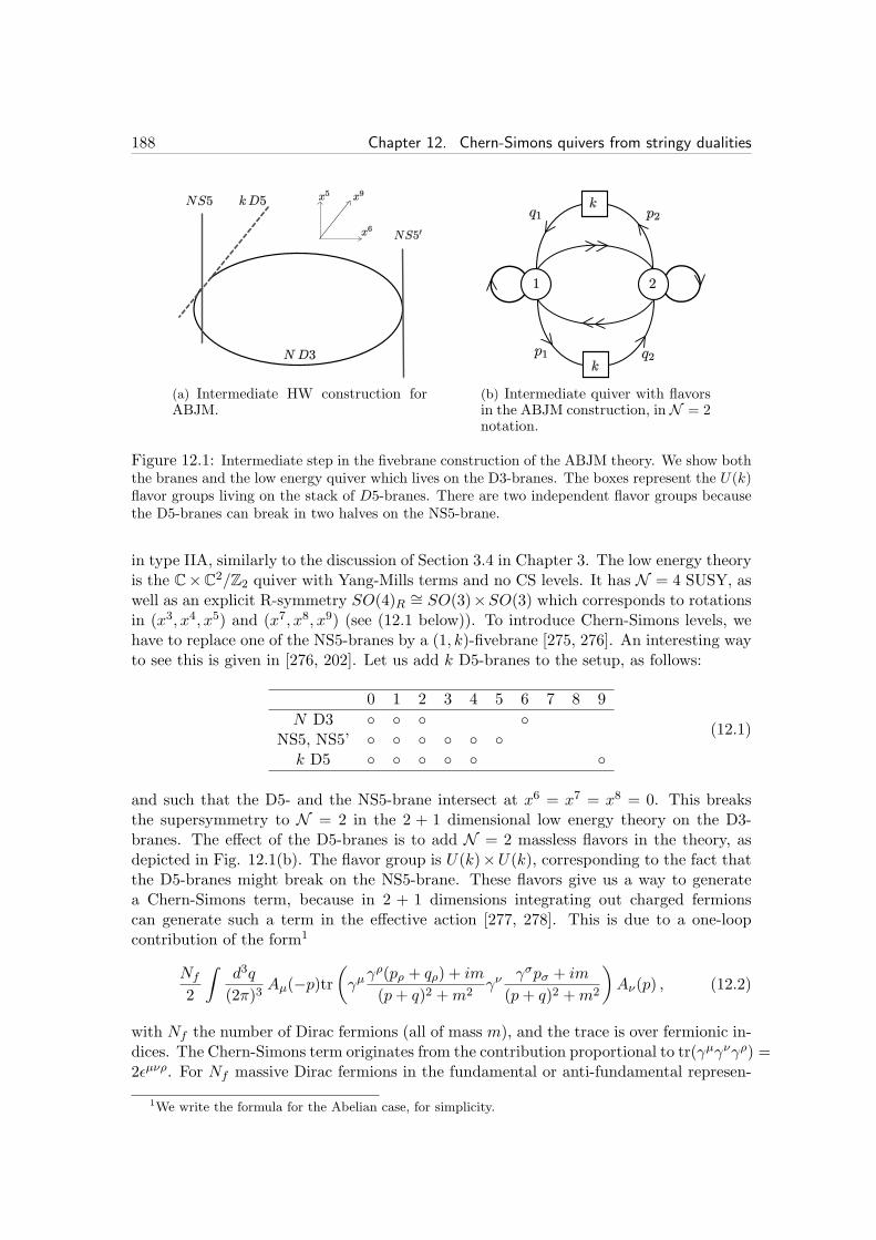
188 Chapter 12. Chern-Simons quivers from stringy dualities
(a) Intermediate HW construction forABJM.
(b) Intermediate quiver with flavorsin the ABJM construction, in N = 2notation.
Figure 12.1: Intermediate step in the fivebrane construction of the ABJM theory. We show boththe branes and the low energy quiver which lives on the D3-branes. The boxes represent the U(k)flavor groups living on the stack of D5-branes. There are two independent flavor groups becausethe D5-branes can break in two halves on the NS5-brane.
in type IIA, similarly to the discussion of Section 3.4 in Chapter 3. The low energy theoryis the C×C
2/Z2 quiver with Yang-Mills terms and no CS levels. It has N = 4 SUSY, aswell as an explicit R-symmetry SO(4)R ∼= SO(3)×SO(3) which corresponds to rotationsin (x3, x4, x5) and (x7, x8, x9) (see (12.1 below)). To introduce Chern-Simons levels, wehave to replace one of the NS5-branes by a (1, k)-fivebrane [275, 276]. An interesting wayto see this is given in [276, 202]. Let us add k D5-branes to the setup, as follows:
0 1 2 3 4 5 6 7 8 9
N D3 NS5, NS5’ k D5
(12.1)
and such that the D5- and the NS5-brane intersect at x6 = x7 = x8 = 0. This breaksthe supersymmetry to N = 2 in the 2 + 1 dimensional low energy theory on the D3-branes. The effect of the D5-branes is to add N = 2 massless flavors in the theory, asdepicted in Fig. 12.1(b). The flavor group is U(k)×U(k), corresponding to the fact thatthe D5-branes might break on the NS5-brane. These flavors give us a way to generatea Chern-Simons term, because in 2 + 1 dimensions integrating out charged fermionscan generate such a term in the effective action [277, 278]. This is due to a one-loopcontribution of the form1
Nf
2
∫d3q
(2π)3Aµ(−p)tr
(
γµγρ(pρ + qρ) + im
(p+ q)2 +m2γν
γσpσ + im
(p+ q)2 +m2
)
Aν(p) , (12.2)
with Nf the number of Dirac fermions (all of mass m), and the trace is over fermionic in-dices. The Chern-Simons term originates from the contribution proportional to tr(γµγνγρ) =2ǫµνρ. For Nf massive Dirac fermions in the fundamental or anti-fundamental represen-
1We write the formula for the Abelian case, for simplicity.
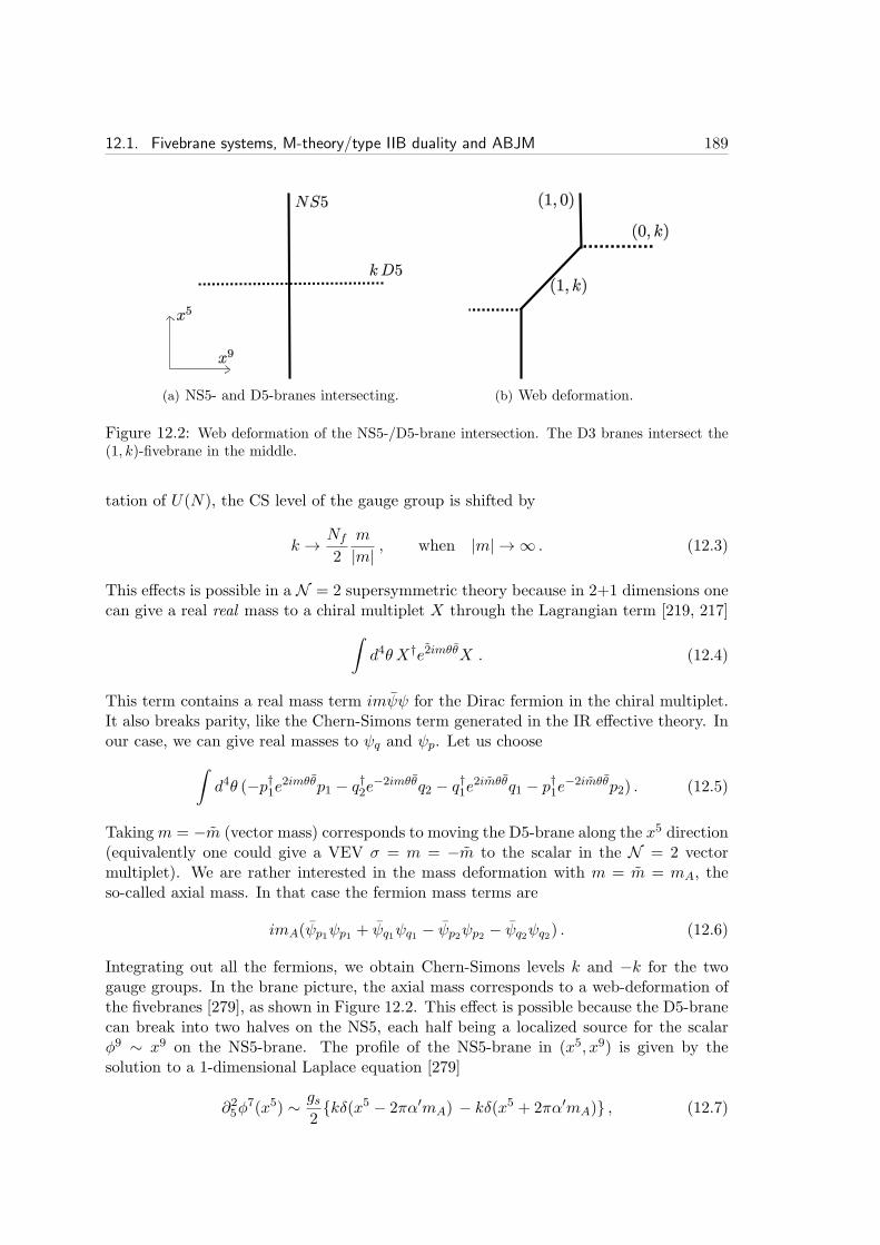
12.1. Fivebrane systems, M-theory/type IIB duality and ABJM 189
(a) NS5- and D5-branes intersecting. (b) Web deformation.
Figure 12.2: Web deformation of the NS5-/D5-brane intersection. The D3 branes intersect the(1, k)-fivebrane in the middle.
tation of U(N), the CS level of the gauge group is shifted by
k → Nf
2
m
|m| , when |m| → ∞ . (12.3)
This effects is possible in a N = 2 supersymmetric theory because in 2+1 dimensions onecan give a real real mass to a chiral multiplet X through the Lagrangian term [219, 217]
∫
d4θ X†e2imθθX . (12.4)
This term contains a real mass term imψψ for the Dirac fermion in the chiral multiplet.It also breaks parity, like the Chern-Simons term generated in the IR effective theory. Inour case, we can give real masses to ψq and ψp. Let us choose
∫
d4θ (−p†1e2imθθp1 − q†2e−2imθθq2 − q†1e2imθθq1 − p†1e−2imθθp2) . (12.5)
Takingm = −m (vector mass) corresponds to moving the D5-brane along the x5 direction(equivalently one could give a VEV σ = m = −m to the scalar in the N = 2 vectormultiplet). We are rather interested in the mass deformation with m = m = mA, theso-called axial mass. In that case the fermion mass terms are
imA(ψp1ψp1 + ψq1ψq1 − ψp2ψp2 − ψq2ψq2) . (12.6)
Integrating out all the fermions, we obtain Chern-Simons levels k and −k for the twogauge groups. In the brane picture, the axial mass corresponds to a web-deformation ofthe fivebranes [279], as shown in Figure 12.2. This effect is possible because the D5-branecan break into two halves on the NS5, each half being a localized source for the scalarφ9 ∼ x9 on the NS5-brane. The profile of the NS5-brane in (x5, x9) is given by thesolution to a 1-dimensional Laplace equation [279]
∂25φ7(x5) ∼ gs
2kδ(x5 − 2πα′mA) − kδ(x5 + 2πα′mA) , (12.7)

190 Chapter 12. Chern-Simons quivers from stringy dualities
(a) N = 3 brane setup. (b) Elliptic CS-quiver.
Figure 12.3: N = 3 brane setup and the corresponding elliptic CS-quiver.
which gives Figure 12.2(b). The brane stretching at angle must be a (1, k)-fivebranebound state, because of flux conservation. The angle θ between the NS5- and the (1, k)is fixed by N = 2 supersymmetry in term of the type IIB axio-dilaton; when C0 = 0, wehave tan θ = gsk, as follows from (12.7). Sending mA → ∞, we are left with only the(1, k)-fivebrane, toegether with the remaining NS5’-brane. The low energy theory is theC × C
2/Z2 quiver with N = 2 Chern-Simons terms. We can obtain a N = 3 theory byadding a mass term m = ±k/8π for the complex adjoint chiral superfields Φ1, Φ2, whichis the N = 3 completion of the Chern-Simons interaction (we already encountered it atthe end of Chapter 9). This corresponds to a rotation of the NS5’-brane by a angle θ inboth the planes (x3, x7) and (x4, x8). Thus we have reconstructed the Yang-Mills-Chern-Simons UV completion of the ABJM theory from a type IIB brane setup.
This N = 3 brane setup has a simple M-theory dual, which is obtained by T-dualizingalong x6 and further uplifting to M-theory. In fact the hyper-Kahler metric of the dualM-theory geometry is precisely known [280], in term of a U(1)2 fibration over R
6. TheD3-branes are simply M2-branes on that geometry. These hyper-Kahler spaces are inter-esting 8 dimensional generalizations of a multi-Taub-NUT. The IR limit on the M2-branesamounts to zooming on the origin of the geometry, which has the effect of washing outthe effect of the Taub-NUT-like structure (the topology R
6 × S1 × S1 at infinity) andleaving us with a conical singularity at the origin.
Here we are simply interested in the complex structure of such geometries, with theimplicit understanding that we perform the above near-horizon limit, so that we obtaina conical hyper-Kahler metric. In the case of ABJM, the complex structure is C4/Zk. Inthe low energy theory only the Chern-Simons interactions remain.
12.1.1 N = 3 generalizations
This fivebrane realization of ABJM is easily generalized to a family of N = 3 quiver-Chern-Simons theories [281, 282], the so-called elliptic quivers. The brane configurationconsists of G fivebranes along a circle, as shown in Figure 12.3(a). The i-th brane has

12.1. Fivebrane systems, M-theory/type IIB duality and ABJM 191
charge (1, qi), and it spans the directions:
0 1 2 6 [3,7] [4,8] [5,9]
(1, qi)-brane θi/ θi/ θi/N D3
(12.8)
In this table we also included N D3-branes along x6. The orientation angle θi in eachplane (xi, xi+4) is such that tan θi = qi (for τ = i). The quiver (Fig. 12.3(b)) is made ofG gauge groups connected through a single loop. The Lagrangian is similar to the one of(11.1), with the N = 3 superpotential
W =G∑
i=1
2π
ki(AiBi −Bi−1Ai−1)
2 . (12.9)
The Chern-Simons levels (k1, · · · , kG) are determined in term of the fivebrane charges,
ki = qi − qi−1 , ⇔ qi =∑i
j=1kj . (12.10)
Note that a transformation which shifs all the q’s by a constant does not affect the CSlevels. We can choose the last fivebrane (i = G) to be a NS5-brane (by performing aSl(2,Z) transformation τ → 1/(1− qGτ)).
12.1.2 Moduli space and hyper-toric geometry
In [282], it was shown that the moduli space of this N = 3 quiver is a hyper-toric variety.Let us briefly explain this geometric construction. Hypertoric geometry is a generalizationof the Kahler approach to toric geometry, jumping from the field C to H (the quaternions).A nice account is provided in [283]. A hypertoric variety is a 4n–real-dimensional varietyadmitting a (C∗)n torus action (much like a 2n-real-dimensional toric variety does), whichis hyper-Kahler (i.e. admits 3 complex structures satisfying the quaternion algebra).2
Let us define a set of d vectors (ui) in a lattice N ∼= Zn, defining a linear map
β ≡ (u1, · · ·ud) : Rd → Rn (12.11)
and define the charge covectors (Q1, · · ·Qd−n) as spanning the kernel of β. Then thevariety M(u, λ) is defined as the hyper-Kahler quotient
M(u, λ) = Hd///G, (12.12)
with G = kerβ. Here λ stands for hyper-Kahler parameters. Choosing one of the 3complex structures, one can split each quaternion variable h as h = (z, w) ∈ C
2. Thetorus C∗ acts on h as
t · h = (tz, t−1w) (12.13)
2We see that, confusingly, a hyper-toric variety is generally not toric, since the typical isometry of ahyper-toric variety of complex dimension 2n is U(1)n instead of U(1)2n.
192 Chapter 12. Chern-Simons quivers from stringy dualities
Hence, we have Hn ∼= (zi, wi). The quotient is taken by defining a triplet of moment
maps
µRa =1
2
∑
i
Qia(|zi|2 − |wi|2
), (12.14)
µCa =∑
i
Qiaziwi . (12.15)
for each U(1)a, a = 1, · · · d− n and setting
µRa = λRa , µCa = λCa . (12.16)
where the constants λ are the hyper-Kahler parameters. To obtain a cone, we need toset λ = 0. Then, we quotient by the U(1)d−n gauge symmetry. There is an importantsubtlety, much like for the toric case, in defining kerβ. If (u) only generate a sublatticeN ′ of N , then we have to quotient also by the discrete group Γ = N/N ′:
G = U(1)d−n × Γ . (12.17)
In our case, we set n = 2, so that the space is eight dimensional. The hyper-toricvariety M(u, λ) is then defined by a set of d = G integer vectors on the plane. Inthat case, the Theorem (4.1) of [283] says that M(u, 0) is the Riemannian cone overa compact 3-Sasakian manifold if and only if: (i) every subset of two vectors in (u) islinearly independant and (ii) every single vector in (u) is a part of a Z-basis of Z2.
If condition (ii) of the theorem does not hold, but instead one generates a sublatticeof Z2, the hyper-Kahler cone has non-isolated quotient singularities.
The crucial observation of [282] is that the metric β of vectors in the hyper-toric fancorresponds to the charges of the (p, q) branes in the type IIB setup. For the setup ofFig. 12.3(a), we have
β = (u1, · · ·uG) =(1 1 · · · 1 1q1 q2 · · · qG−1 0
)
. (12.18)
This characterization of the moduli space in term of the hyper-Kahler quotient (12.12)allows to use many known mathematical results to study the associated AdS/CFT cor-respondance. It also suggests interesting generalizations, to which we now turn.
12.2 N = 3 Flavors in ABJM: the Gaiotto-Jafferis construc-
tion
The generic hyper-toric geometry characterized by
β =
(p1 p2 · · · pdq1 q2 · · · qd
)
(12.19)
can be realized as a type IIB setup involving (p, q) branes [280]. However, we have almostno understanding of the field theory on D3-branes suspended between arbitrary (p, q)-branes, so we cannot use that construction to study explicit instances of the AdS4/CFT3
correspondence.
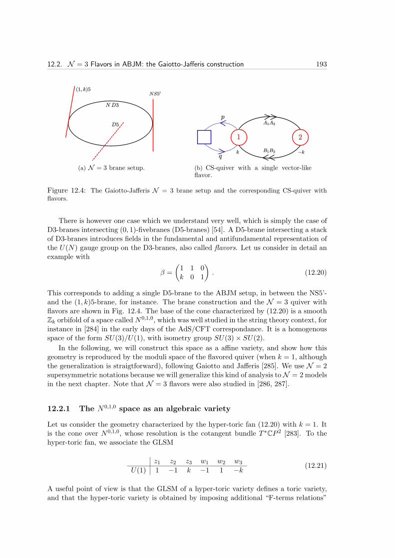
12.2. N = 3 Flavors in ABJM: the Gaiotto-Jafferis construction 193
(a) N = 3 brane setup. (b) CS-quiver with a single vector-likeflavor.
Figure 12.4: The Gaiotto-Jafferis N = 3 brane setup and the corresponding CS-quiver withflavors.
There is however one case which we understand very well, which is simply the case ofD3-branes intersecting (0, 1)-fivebranes (D5-branes) [54]. A D5-brane intersecting a stackof D3-branes introduces fields in the fundamental and antifundamental representation ofthe U(N) gauge group on the D3-branes, also called flavors. Let us consider in detail anexample with
β =
(1 1 0k 0 1
)
. (12.20)
This corresponds to adding a single D5-brane to the ABJM setup, in between the NS5’-and the (1, k)5-brane, for instance. The brane construction and the N = 3 quiver withflavors are shown in Fig. 12.4. The base of the cone characterized by (12.20) is a smoothZk orbifold of a space called N0,1,0, which was well studied in the string theory context, forinstance in [284] in the early days of the AdS/CFT correspondance. It is a homogenousspace of the form SU(3)/U(1), with isometry group SU(3)× SU(2).
In the following, we will construct this space as a affine variety, and show how thisgeometry is reproduced by the moduli space of the flavored quiver (when k = 1, althoughthe generalization is straigtforward), following Gaiotto and Jafferis [285]. We use N = 2supersymmetric notations because we will generalize this kind of analysis toN = 2 modelsin the next chapter. Note that N = 3 flavors were also studied in [286, 287].
12.2.1 The N0,1,0 space as an algebraic variety
Let us consider the geometry characterized by the hyper-toric fan (12.20) with k = 1. Itis the cone over N0,1,0, whose resolution is the cotangent bundle T ∗
CP 2 [283]. To thehyper-toric fan, we associate the GLSM
z1 z2 z3 w1 w2 w3
U(1) 1 −1 k −1 1 −k (12.21)
A useful point of view is that the GLSM of a hyper-toric variety defines a toric variety,and that the hyper-toric variety is obtained by imposing additional “F-terms relations”
194 Chapter 12. Chern-Simons quivers from stringy dualities
(12.15). In our example, we have the following 9 gauge invariant complex variables:
x0 = z1z2, x1 = z1w1, x2 = z1w3,x3 = z3z2, x4 = z3w1, x5 = z3w3,x6 = w2z2, x7 = w2w1, x8 = w2w3,
(12.22)
and the “intermediate” 5-complex-dimensional toric variety is defined by
x0x4 − x1x3 = 0, x0x5 − x2x3 = 0, x0x7 − x1x6 = 0,x0x8 − x2x6 = 0, x1x5 − x2x4 = 0, x1x8 − x2x7 = 0,x3x7 − x4x6 = 0, x3x8 − x5x6 = 0, x4x8 − x5x7 = 0,
(12.23)
Moreover, we have an additional “F-term” condition µC = 0:
x1 + x5 − x6 = 0 , (12.24)
which allows to eliminate x5, say, in term of the other variables. For k > 1, the story issimilar, although more tedious to write down.
12.2.2 Recovering N0,1,0 from the quantum chiral ring
Consider now the theory of Figure 12.4. We have the chiral superfields fields p and q, inthe fundamental and anti-fundamental of the first gauge group, and the bifundamentalfields Ai, Bi as in ABJM. The superpotential is fixed by N = 3 supersymmetry,
W =2π
k(A1B1 −A2B2 + pq)2 − 2π
k(B2A2 −B1A1)
2 . (12.25)
For p = q = 0, it reduces to the ABJM superpotential (11.3). The explicitly realizedglobal symmetry is
SU(2)R × SU(2)F × U(1)B . (12.26)
The “baryonic” symmetry U(1)B rotates p and q with opposite charges. When k = 1,SU(2)F is enhanced to SU(3) due to non-perturbative effects, as we will show. We focuson the Coulomb branch, for which p = q = 0. We also consider only the abelian theory,in which case there is no F-term relations. At first sight it is not clear how to recover thealgebraic construction of the last subsection from the quiver theory with a single flavor,since it would seem that the Coulomb branch is the same as in ABJM. However, we needto consider more carefully the monopole operators. They have the same electric chargesas in ABJM. However, they now have a non-vanishing R-charge. This follows directlyfrom the discussion of Chapter 10, equation (10.34). Since the fermions ψp, ψq in thechiral multiplets p, q have R-charge −1
2 (in N = 3 theories the R-charges are the classicalones), the induced R-charge of the monopole operators is
R(T (n)) = −|n|2
(R(ψp) +R(ψp)) =|n|2. (12.27)
This means that the bare monopole operators operators T , T carrying ±1 units of mag-netic flux along U(1)D have dimension 1
2 , the same dimension as the chiral field Ai, Bi.This allows to construct an enhanced SU(3) global symmetry, by forming SU(3) triplets
(A1, A2, T ), (B1, B2, T ) . (12.28)
12.3. Stringy derivation of N = 2 Chern-Simons quivers 195
The abelian chiral ring is generated by the following gauge invariant operators:
X0 = A1B1, X1 = A1B2, X2 = A1T ,
X3 = TB1, X4 = TB2, X5 = T T ,
X6 = A2B1, X7 = A2B2, X8 = A2T ,
(12.29)
The correspondence with the hyper-toric description is clear:
z1 z2 z3 w1 w2 w3
A1 B1 T B2 A2 T(12.30)
The U(1) of the gauge linear model (12.21) is the U(1)b of the quiver 3. To obtainC(N0,1,0), the crucial relation is the F-term relation (12.24). In the field theory language,it reads
T T = A2B1 −A1B2 . (12.31)
This is a completely quantum relation. As explained in Chapter 10, the OPE T T can apriori contain any operator with the same quantum numbers. Since T T has dimension1 and is a singlet under SU(2)F , the only possible operator which could have appearedwas ǫijAiBj . That it indeed appears was argued in [285]. In the next Chapter we willconjecture a similar OPE in a N = 2 setup, allowing us to consider generic flavors inN = 2 quivers. Before we do that, we will now introduce another string theory derivationof a larger class of AdS4/CFT3 dualities.
12.3 Stringy derivation of N = 2 Chern-Simons quivers
For some of the N = 2 quivers proposed in the litterature, such as the ones reviewedin the last chapter, it is not known how or whether they can be constructed from stringtheory. This puts the associated AdS4/CFT3 duality conjectures on a less firm groundthan in the case of the N = 3 quivers of this chapter, which do have a clear string theoryderivation in term of D3- and fivebranes.
In this section we review and slightly clarify a type IIA derivation of the N = 2 Chern-Simons quiver associated to M2-branes on any toric Calabi-Yau fourfold singularity [258].It will provide use with a better understanding as to why M2-brane quivers look like D-brane quivers. This derivation was first explicitly considered by Aganagic [258]. Therelation between the CY4 geometric moduli space of a 3d quiver CS theory and theCY3 = CY4//U(1)M mesonic moduli space of a 4d gauge theory with the same quiverand superpotential was pointed out before in [282, 244, 245].
We consider toric Calabi-Yau singularities only. The basic idea of [258] is to write atoric CY4 cone as line fibration over a toric Calabi-Yau threefold,
C → CY4 → CY3 . (12.32)
The fibration structure of the S1 ⊂ C corresponds to the fibration structure of the M-theory circle. Reducing along this circle, the type IIA setup is the CY3 fibered over a realline. M2-branes become D2-branes on the CY3 in type IIA, in which case we know their
3Indeed for Chern-Simons level k, the U(1) charge of the monopole operator is ±k, as in (12.21).

196 Chapter 12. Chern-Simons quivers from stringy dualities
associated quiver very well. Moreover the non-trivial fibration leads to Chern-Simonsinteraction in the field theory, as we will review.
We stress again that there is generally several ways to choose the M-theory circle,corresponding to several different weak string coupling limits of M-theory.
12.3.1 CY4 as a U(1) fibration
Let us explain how to rewrite a toric CY d-fold as a (possibly singular) U(1) fibrationover a manifold, which in turn is the fibration of a toric CY (d − 1)-fold along a realline, with Kahler moduli that vary linearly along the line. We begin by following theexposition in [258], but we further stress the regularity conditions one has to impose onthe choice of fibration structure.
Consider a toric CY d-fold, realized as the moduli space of a gauged linear sigma-model (GLSM). There are R+ d chiral superfields φs with s = 1, . . . , R+ d, and R U(1)gauge groups with integer charges Qas (of maximal rank) with a = 1, . . . , R. The CYcondition is
∑
sQas = 0 for all a. The number R + d of fields can be taken to be equal
to the number of dots in the (d− 1)-dimensional toric diagram. Then the charge matrixQas encodes the R linear relations
∑
sQas ~vs = 0 between the vectors ~vs in the toric fan.
The CY Yd is simply the Kahler quotient CR+d//U(1)R, which corresponds to imposingthe moment map (D-term) equations
∑
sQas |φs|2 = ra (12.33)
and quotienting by the gauge group
φs → ei∑
a λaQas φs . (12.34)
The moment map (or FI) parameters ra are the resolution parameters of Yd. We will bemainly interested in the conical case ra = 0. Moreover, for each a the charges Qas can betaken coprime without loss of generality.
To exhibit the fibered structure, we add the complex variable r0 + iθ0 and choose aset of charges Q0
s satisfying the CY condition∑
sQ0s = 0. Then we impose one more
equation and divide by one more gauge symmetry:∑
sQ0s |φs|2 = r0 ; θ0 → θ0 + λ , φs → eiλQ
0s φs . (12.35)
It is easy to check that the manifold is the same as before: using (12.35) r0 can be elimi-nated while θ0 can be gauged away (without leaving any residual gauge transformation).
On the other hand, we can fix r0 and think of θ0 as a U(1) fibration. The basemanifold Yd−1 is then the Kahler quotient CR+d//U(1)R+1:
∑
sQ0s |φs|2 = r0 ,
∑
sQas |φs|2 = ra ∀ a = 1, . . . , R , (12.36)
modded out byφs → eiλQ
0s + i
∑
a λaQas φs . (12.37)
Yd−1 is toric and Calabi-Yau. Moreover, Yd−1 is fibered over the real line r0, with aparticular combination of the resolution parameters (set by Q0
s) varying linearly with r0.The tip of Yd is at r0 = 0.

12.3. Stringy derivation of N = 2 Chern-Simons quivers 197
Figure 12.5: Projection of the toric diagram of C4 -left- to one of the conifold -right-.
Projecting the toric diagram. Given the set of charges Qas , the toric fan ofYd is given by R + d primitive vectors ~vs in Z
d which solve the R linear conditions∑
sQas ~vs = 0 for all a = 1, . . . , R. We can collect the vectors as columns of a matrix
(GK)is, with i = 1, . . . , d, of maximal rank. Then
Qas (GTK)si = 0 (12.38)
and the rows of GK span the kernel of Qas as a map from RR+d to R
R. We can use atransformation of SL(d,Z) to map the vectors to ~vs = (1, ~ws). The same equation canbe used to obtain the charges of a GLSM, given the matrix GK of all vectors in the toricfan.
The toric diagram of Yd−1 can be obtained in the same way. We add the extracondition
∑
sQ0s ~vs = 0. The vectors ~vs do not satisfy it, because the rows of (GK)
is are
linearly independent. In order to satisfy the extra relation, we must project the vectorson a hyperplane in such a way that the linear combination4
~vM ≡ primitive∑
sQ0s ~vs (12.39)
vanishes, that is a hyperplane orthogonal to ~vM . Notice that the CY condition on Q0s
plus the particular chosen frame ~vs = (1, ~ws) assures that ~vM = (0, ~wM ). To makethe projection clearer, we can perform an SL(d− 1,Z) transformation that maps ~vM to(0, . . . , 0, 1), and changes the toric diagram of Yd accordingly. Then the toric diagram ofYd−1 is obtained from the one of Yd with the “vertical” projection that forgets the lastcomponent, as in Figure 12.5.
Fixed points. The reduction Yd−1 = Yd//U(1)M can always be done. However,whenever the U(1)M fiber degenerates, we should expect some extra object or singularityin the type IIA background, on top of any possible geometric toric singularity (evennon-isolated) of Yd−1.
A first class of singularities arises from loci where the fiber U(1)M shrinks:
• each strictly external dot ~vs in the (d − 1)-dimensional toric diagram of Yd is aconical toric divisor (complex codimension one) where the circle ~vs shrinks;
• each external edge vsr connecting two adjacent dots ~vs and ~vr is a conical codimen-sion 2 surface where the span in U(1)d of the two circles shrinks;
4We mean that ~vM is the primitive vector in Zd which is parallel to
∑
sQ0s ~vs.
198 Chapter 12. Chern-Simons quivers from stringy dualities
• each external polyhedron vs1...sn of dimension n−1 constructed between the strictlyexternal dots ~vs1 , . . . , ~vsn is a conical codimension n surface where the span in U(1)d
of the n circles shrinks.
In order to have a non-singular Kahler quotient for the projection, we should make surethat the circle ~vM is not contained in any of the spans above (the first case is automaticallyexcluded). Practically, we require ~wM not to be parallel to any external sub-object in theconvex polyhedron of the (d − 1)-dimensional toric diagram. We stress that we are notworried about singularities in the quotient Yd−1, but rather about degenerations of thefiber.
There is a second class of possible singularities, where the U(1)M fiber degeneratesto U(1)/Zp for some p. This happens if some of the charges in Q0
s have modulus largerthan 1. In this case, there could be a conical surface where the fiber U(1)M degenerates:we have to make sure that the only point where this happens is the tip of Yd.
The case of CY4. Specializing to the case of interest – Y4 and Y3 = Y4//U(1)M–, whenever none of the singularities above arises in the quotienting, we are sure thatthe reduction of M-theory on Y4 along U(1)M gives a pure IIA background (to which thearguments in [258] can be applied), without extra objects on top of it.
In particular, we should make sure that: 1) there are no external edges in the 3d toricdiagram parallel to ~wM ; 2) there are no external faces parallel to ~wM ; 3) once ~wM isexpressed as an integer sum of the ~ws in the 3d toric diagram, if some coefficients havemodulus larger than 1, the fiber does not degenerate outside the tip of Y4.
On the contrary, whenever the fiber degenerates, we should expect some extra objectsin type IIA that have to be taken into account. In the next Chapter, we will study whathappens if the fiber shrinks on a complex codimension-two submanifold of the four-fold(giving rise to D6-branes). The other cases deserve a separate study.
12.3.2 Chern-Simons quivers from type IIA
By the above construction, we have a duality between M2-branes at the tip of a CY4 andD2-branes on a CY3 fibered over R (the D2-branes sit at r0 = 0 and at the tip of thethreefold). According to (12.35), the coordinate r0 is a Kahler modulus of the Calabi-Yauthreefold. More generally, we can consider
∑
sQ0s |φs|2 = hr0 ; θ0 → θ0 + hλ , φs → eiλQ
0s φs , (12.40)
for h some positive integer. This changes Yd to Yd/Zh, corresponding to shrinking the θ0circle by a factor of h. This is usually by such a further orbifold that a weakly coupledtype IIA background is obtained, as in the ABJM case. The gauge invariant vielbeincharacterizing the M-theory fibration is
dθ0 + i∑
sqs dφs/φs , (12.41)
with qs such that∑
sqsQ
as = 0 ,
∑
sqsQ
0s = h . (12.42)
This identifies the connection∑
s qsdφs/φs as the RR 1-form C1. The RR 2-form fluxF2 = dC1 is [258]
F2 =∑
sqs ωs , with ωs = δ2(φs)dφs ∧ dφs (12.43)
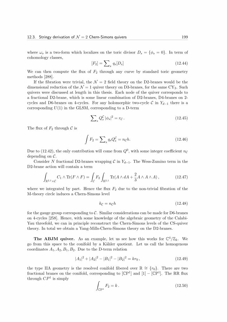
12.3. Stringy derivation of N = 2 Chern-Simons quivers 199
where ωs is a two-form which localizes on the toric divisor Ds = φs = 0. In term ofcohomology classes,
[F2] =∑
sqs[Ds] (12.44)
We can then compute the flux of F2 through any curve by standard toric geometrymethods [288].
If the fibration were trivial, the N = 2 field theory on the D2-branes would be thedimensional reduction of the N = 1 quiver theory on D3-branes, for the same CY3. Suchquivers were discussed at length in this thesis. Each node of the quiver corresponds toa fractional D2-brane, which is some linear combination of D2-branes, D4-branes on 2-cycles and D6-branes on 4-cycles. For any holomorphic two-cycle C in Yd−1 there is acorresponding U(1) in the GLSM, corresponding to a D-term
∑
sQCs |φs|2 = rC . (12.45)
The flux of F2 through C is
∫
F2 =∑
sqsQ
Cs = nCh. (12.46)
Due to (12.42), the only contribution will come from Q0, with some integer coefficient nCdepending on C.
Consider N fractional D2-branes wrapping C in Yd−1. The Wess-Zumino term in theD2-brane action will contain a term
∫
R2,1×CC1 ∧ Tr(F ∧ F ) =
∫
CF2
∫
R2,1
Tr(A ∧ dA+2
3A ∧A ∧A) , (12.47)
where we integrated by part. Hence the flux F2 due to the non-trivial fibration of theM-theory circle induces a Chern-Simons level
kC = nCh (12.48)
for the gauge group corresponding to C. Similar considerations can be made for D6-braneson 4-cycles [258]. Hence, with some knowledge of the algebraic geometry of the Calabi-Yau threefold, we can in principle reconstruct the Chern-Simons levels of the CS-quivertheory. In total we obtain a Yang-Mills-Chern-Simons theory on the D2-branes.
The ABJM quiver. As an example, let us see how this works for C4/Zk. We
go from this space to the conifold by a Kahler quotient. Let us call the homogenouscoordinates A1, A2, B1, B2. Due to the D-term relation
|A1|2 + |A2|2 − |B1|2 − |B2|2 = kr0 , (12.49)
the type IIA geometry is the resolved conifold fibered over R ∼= r0. There are twofractional branes on the conifold, corresponding to [CP1] and [1] − [CP1]. The RR fluxthrough CP 1 is simply ∫
CP1
F2 = k . (12.50)

200 Chapter 12. Chern-Simons quivers from stringy dualities
Hence the Chern-Simons theory is the conifold quiver with Chern-Simons levels (k,−k),as expected.
The construction of [258] gives a neat explanation of the string theory origin of Chern-Simons quiver. The explanation of the quiver structure of ABJM and its generalizationsboils down to well known properties of D-branes. This is worth stressing, because it meansthat the quiver, by itself, does not contain any properties which would be “intrinsic” tothe M2-brane. In particular, many different quivers will be dual (generalizing 3d mirrorsymmetry [208]) if they correspond to the same M-theory geometry. The situation isdifferent from the case of Seiberg duality for D3-brane quivers, because in that latter casethe dualities are well understood as a reshuffling of the fractional branes. Here there is nosuch “mechanical” understanding of the M-theory duality, because we still do not haveany direct control over the M2-brane degrees of freedom. Instead we have to rely on adual picture, either in type IIB like in the first part of this chapter, or in type IIA like inthis section.
In the next chapter we will generalize the type IIA derivation of N = 2 M2-branetheories to the case where the M-theory Calabi-Yau fourfold contains non-isolated singu-larities in complex codimension two.
Chapter 13
Flavors in N = 2 toricChern-Simons quivers
In this second Part of the thesis we have discussed in some detail various theories whichare conjectured to describe the low energy theory on M2-branes sitting on some eightdimensional cone. Each such proposal leads to a new instance of a AdS4/CFT3 duality,although in the N = 2 case there is generally no weak coupling limit in the field theory(similarly to the case of N = 1 quiver SCFTs in 4d). Almost all of the field theorywhich we reviewed involve gauge groups with only adjoint and bifundamental matter,like conformal quiver gauge theories in 3+1 dimensions. In the previous Chapter we haveseen that this is not a coincidence.
The string theory understanding of the correspondence leads to natural generaliza-tions. It has been proposed recently that the dynamics of M2-branes on some hyper-Kahler cones (N = 3 SUSY) is described by flavored quiver CS theories, includingmatter in the fundamental and antifundamental representation of the gauge groups[285, 286, 287]; we reviewed such a proposal in section 12.2 in the last chapter. Fla-vors were further studied in [289, 290, 291].
We aim to extend this program to M2-branes probing toric CY4 singularities. ThisChapter is entirely based on [3], written in collaboration with Stefano Cremonesi andFrancesco Benini. A similar approach was advocated by Daniel L. Jafferis [292], withwhom we coordinated the release of the arXiv preprints. The later work [292] also givesa discussion of some non-toric examples.
13.1 Motivation and overview
One of the problems we want to address is what happens when the fourfold has con-ical complex codimension-two singularities, which means that the base H7 itself hascodimension-two singularities: this is related to the addition of flavors – fields in thefundamental representation of the gauge groups. An Ah−1 complex codimension-two sin-gularity locally looks like C
2 × C2/Zh. M-theory on such a background develops SU(h)
gauge fields living along the singularity, and by the AdS/CFT map there must be anSU(h) global symmetry in the boundary theory. Many models in the literature have
201
202 Chapter 13. Flavors in N = 2 toric Chern-Simons quivers
such singularities, however the large non-Abelian symmetry is not manifest. It is naturalto look for a description in terms of flavors in the quiver theory.
Another way to understand the issue is to select a U(1) isometry of the CY4 thatpreserves the holomorphic 4-form Ω4, quotient the geometry by Zk ⊂ U(1) and reducealong the circle to type IIA. The resulting background is a warped product AdS4×wH6,with RR fluxes and varying dilaton. If 1 ≪ k ≪ N1/5 type IIA is weakly coupled,whereas for k ≫ N one expects a Lagrangian description for the 2-brane theory withweakly coupled gauge groups. If the U(1) circle shrinks on a complex codimension-twosurface in the CY4, we get D6-branes in the type IIA background, filling AdS4 andwrapping a 3-cycle in H6. In fact, C2 ×C
2/Zh is the complex structure of a multi-Taub-NUT which, if reduced along its U(1) isometry, gives rise to h D6-branes. It is knownthat the D2-D6 system introduces flavors in the theory living on D2-branes, as happensin the N = 3 case [285, 286, 287].
A more systematic tool to derive the theory on M2-branes probing a CY4 geometry isthe Kahler quotient approach [258] which we reviewed in the last Chapter. This approachis powerful because it does not need metric details of the four-fold, but only algebraicgeometric data. When the U(1) fiber shrinks on codimension-two submanifolds of theCY4, we get D6-branes wrapping divisors of the CY3, and the theory on M2-branes has thesame quiver and superpotential as the theory on D3-branes on the CY3 in the presence ofD7-branes wrapping the same divisors. For h D7-branes wrapping an irreducible divisor,the effect is that of introducing h pairs of quarks (p, q) coupled via the superpotentialterm
δW = p (divisor equation) q ,
where the divisor equation is written in terms of the bifundamental matter fields in thetheory.
Led by these considerations, we can study what happens if we start with an N = 2quiver Chern-Simons theory, dual to a toric CY4 geometry, and we flavor it. We meanthat we select a subset Xα of bifundamental fields in the quiver, and for each of themwe introduce hα pairs of chiral multiplets (pα, qα) in the (anti)fundamental representationof the gauge groups, coupled by the superpotential term
W =W0 +∑
αpαXαqα ,
W0 being the “unflavored” superpotential. Because of the parity anomaly, this has to beaccompanied by a shift of Chern-Simons levels. A concept of “chirality” is induced byN = 2 supersymmetry, and inherited from four dimensions.
To study the chiral ring and moduli space of this theory, a crucial role is played byBPS diagonal monopole operators T (n) [293, 294, 232, 230, 231, 295, 233, 235]. Due toquantum corrections, they acquire global and gauge charges in the presence of flavors.Generically there is only one possible non-trivial OPE compatible with all the symmetries,that in the Abelian case reads
T T =∏
α(Xα)
hα .
We conjecture that this quantum F-term relation holds, since our results strongly supportthis claim from the AdS/CFT point of view. The moduli space has Higgs and Coulomb

13.2. M-theory reduction and D6-branes : A top-down perspective 203
branches. We show that the geometric branch, in which pα = qα = 0, is described by thematter fields Xa plus the two monopole operators T and T , subject to the classical F-term relations from W plus this quantum F-term relation, modded out by the full gaugegroup U(1)G. The geometric moduli space is still a toric CY4, that we precisely identify.Similar ideas appeared in [296].
The Chapter is organized as follows. In Section 13.2 we start with a top-down per-spective, and analyze the Kahler quotient reduction of M-theory in the presence of KKmonopoles. In Section 13.3 we turn to a bottom-up approach and flavor quiver Chern-Simons theories; their moduli space is studied in Section 13.4. Section 13.5 is devoted todeformations by real and complex masses. In Section 13.6 we work out many examples.
13.2 M-theory reduction and D6-branes : A top-down per-spective
Let us consider M2-branes probing a toric conical Calabi-Yau four-fold Y4 in M-theory.1
We are interested in the type IIA string theory background that one obtains by reducingalong a U(1) isometry, in particular in the case that the four-fold contains KK monopolesand the U(1) shrinks along them. The isometry group of a toric four-fold contains U(1)4.A specific U(1) or more generally R subgroup is the superconformal R-symmetry, whilethe remaining commuting U(1)3F leaves the holomorphic 4-form invariant. Reductionalong a circle in U(1)3F manifestly preserves eight supercharges in type IIA.
The toric data of the four-fold are specified by a Lagrangian U(1)4 fibration over astrictly convex rational polyhedral cone. Each facet of the cone represents a toric divisor.In fact the normal vector to a facet, normalized to have integer components, represents theU(1) cycle that shrinks on the facet. The collection ~vs in Z
4 of the normal vectors to allfacets is called the toric fan. The Calabi-Yau condition is equivalent to the end-points ofall vectors in the toric fan being coplanar; one can then use an SL(4,Z) transformationto rewrite them as ~vs = (1, ~ws), with ~ws vectors in Z
3. The information encodedin the toric fan can be summarized by the 3d toric diagram: a 3d convex polyhedronwhose strictly external points are ~ws. We will call strictly external, among the externalpoints, a point which does not lie along a line connecting two external points – thismeans that strictly external points are not inside an edge nor a face of the toric diagram.Each strictly external point represents a conical toric divisor. The elements (0, 1, 0, 0),(0, 0, 1, 0), (0, 0, 0, 1) in the Z
4 ambient space of the toric fan generate the flavor U(1)3Fsymmetry group that commutes with the R-symmetry.
Over the intersection of two adjacent facets, two U(1) cycles in the fiber shrink.Suppose that the shrinking cycles are (1, x, y, z) and (1, x, y, z + 1) (two points verti-cally aligned) in Z
4: at the intersection of the two facets the U(1)M cycle (0, 0, 0, 1),linear difference of the previous ones, shrinks as well. This happens along a complexcodimension-two conical submanifold of the four-fold, and one can locally view the M-theory background as a KK monopole for that U(1)M action. Reducing along U(1)M ,one gets a D6-brane on some type IIA background.
As reviewed in section 12.3, the type IIA background can be written as the fibration
1We refer the reader to [297, 62, 298, 4] for a simple introduction to basic facts about toric geometryand its relevance for quiver gauge theories.

204 Chapter 13. Flavors in N = 2 toric Chern-Simons quivers
Figure 13.1: Vertical projection from the 3d toric diagram of Y4 to the 2d toric diagram of Y3.The three aligned points give rise to two D6-branes.
of a CY3 cone Y3 over a real line r0 ∈ R [258]. Degeneration loci of the U(1)M fiber resultin various “objects” in the type IIA background. The toric threefold Y3 is defined by a2d toric diagram which is the projection of the 3d toric diagram to a plane orthogonalto the primitive vector ~vM that represents the cycle U(1)M used for the reduction. Wecan always perform an SL(3,Z) transformation of the 3d toric diagram and map ~vM to(0, 0, 0, 1); then the 2d toric diagram of Y3 is the “vertical” projection of the 3d diagramto the plane z = 0.
In our example, the fact that two adjacent external points2 in the 3d toric diagramproject to the same point (which is then necessarily strictly external) in the 2d toricdiagram, implies the presence of a D6-brane wrapping a toric divisor of the CY3 in typeIIA (spanning the spacetime R
2,1 and localized at r0 = 0). The toric divisor is specifiedby the projected point. More generally, if the 3d toric diagram has a collection of h+ 1aligned adjacent external points (1, x, y, zj) with zj = z, z + 1, . . . , z + h, and we reducealong the U(1)M cycle (0, 0, 0, 1), all h + 1 points project down to the same strictlyexternal point in the 2d toric diagram and give rise to h coincident D6-branes wrappinga toric divisor of the CY3 (see Figure 13.1).
Along the D6-branes lives a U(h) gauge theory, which by the AdS/CFT map corre-sponds to a U(h) global symmetry on the boundary. We could then expect the boundarytheory to admit a description in which such a symmetry is manifest. The same conclu-sion can be reached in M-theory: h+ 1 adjacent external points in the 3d toric diagramindicate h KK monopoles in Y4 (a multi-Taub-NUT geometry), whose complex structureis locally C
2 × C2/Zh; the Ah−1 singularity carries SU(h) gauge fields, besides the U(1)
gauge field from the KK reduction of the M-theory potential C3. More precisely, in thenear core limit the latter U(1) KK mode is non-normalizable – correspondingly in thedual theory the diagonal U(1) in U(h) is actually gauged.
2Points are adjacent if the line connecting them is strictly external, not contained in a face.

13.2. M-theory reduction and D6-branes : A top-down perspective 205
13.2.1 IIA background as a CY3 fibration with D6-branes
The symplectic reduction of Y4 to a CY3 is useful because it allows to exploit all thepowerful techniques available for D3-branes probing toric singularities, to get informationabout the field theory. Given a toric CY3 singularity in type IIB and N D3-branesprobing it, the dual SCFT in 3+1 dimensions can be generically found with the fastinverse algorithm [71] briefly discussed in Chapter 3.3
We want to extend the correspondence of [258] to cases in which the Kahler quotienthas complex dimension-two degeneration loci. To begin with, let us understand what thetoric divisors of Y3 correspond to. Each strictly external point ~p in the 2d toric diagramcorresponds to a toric divisor, to which is associated a collection of Q bifundamentalfields Xηη=1,...,Q in the quiver theory, that have the same charges under all global (butnot gauge) symmetries. The number Q is given by [299]
Q =
∣∣∣∣det
(∆x ∆y∆x′ ∆y′
)∣∣∣∣, (13.1)
where (∆x,∆y) is the vector connecting the strictly external point ~p to the next strictlyexternal point along the perimeter, while (∆x′,∆y′) is the vector connecting ~p to theprevious strictly external point.4 A time-filling D3-brane wrapped on the 3-cycle whichis the radial section of the toric divisor (such embedding is supersymmetric) correspondsto a dibaryonic operator XN
η [300, 297, 301]. Since the 3-cycle has the topology of aLens space with fundamental group ZQ [297], the D3-branes admit a ZQ flat connectionresulting in Q degenerate vacua. They correspond to the Q different dibaryonic operatorsXN
η . An easy way to identify the set of fields is through perfect matchings in the branetiling construction [68, 60, 61, 76].
Instead of wrapping a D3-brane on a radial section, one can wrap h spacetime-fillingD7-branes on the whole toric divisor (this problem has been considered, e.g., in [302,303, 304, 129, 186]). They introduce a U(h) global symmetry in the field theory, and hflavors of chiral fields pη, qη coupled to one of the bifundamental fields Xη through thesuperpotential term W = pηXηqη. A ZQ connection, flat everywhere but at the tip, canbe specified on the D7-branes to distinguish which bifundamental is flavored.
The same discussion holds in type IIA: D6-branes wrapping toric divisors of the CY3
provide chiral flavors to the quiver gauge theory on D2-branes at the tip. Each stack ofh D6-branes introduces a U(h) flavor group (this is not always the case: we will be moreprecise in Section 13.5) and flavor chiral multiplets pki, qjk coupled to a bifundamental
Xij through a superpotential term5
W = TrpkiXijqjk . (13.2)
Here k stands for a flavor group, i, j for gauge groups and fields are in the fundamental(anti-fundamental) of the first (second) index; all indices are contracted. We will jumpbetween the notations Xa and Xij for bifundamental fields. The field Xij is determinedas explained above.
3A huge number of examples has been explicitly worked out, see [62, 298] and references therein.4 Q is more conveniently defined as the modulus of the cross product of two consecutive legs in the
(p, q)-web that is dual to the 2d toric diagram.5We absorb superpotential couplings inside chiral superfields.

206 Chapter 13. Flavors in N = 2 toric Chern-Simons quivers
The D6-branes are localized along R: reducing the cone Y4 their position is r0 = 0.More generally, the position along r0 corresponds to a real mass for the quarks in fieldtheory, and to a partial resolution (or Kahler) parameter in M-theory (see Section 13.5.1).Since D6-branes, possibly with worldvolume flux, are sources for RR fields, the 2- and4-form fluxes on 2- and 4-cycles vanishing at the CY3 singularity jump at r0:
δ
∫
C2
F2 = #(C2, D6) , δ
∫
C4
F4 = #(C4, D6, C(Fwv)4 ) , (13.3)
where the jump depends on the intersection on Y3 between the cycles, the divisor andthe cycle representing the worldvolume flux. This means that moving the D6’s to the leftor to the right of the D2-branes, the CS levels must jump as well. We will study this indetail.
Summarizing, whenever the U(1)M action has codimension-two fixed loci which de-scend in type IIA to D6-branes wrapping divisors of the CY3, the field theory derivedusing the CY3 singularity is actually flavored.
We conclude this section with some comments. Two important differences betweenchiral flavors in AdS5/CFT4 and in AdS4/CFT3 must be borne in mind. Firstly, in 4dgauge theories chiral flavors are constrained by gauge anomaly cancelation, whereas in3d such a constraint does not exist. The dual statement is that D7-branes wrappingdivisors are constrained by RR C0 tadpole cancelation, whilst D6-branes are not becausethe RR F2 flux can escape to infinity along the transverse non-compact real line. Thenumber of fundamental minus anti-fundamental fields for a gauge group in 3d need notvanish: if it is odd, the parity anomaly requires the presence of half-integral CS levels[305, 277, 278]. Secondly, in general the addition of flavors to an AdS5/CFT4 pair breaksconformal invariance and the RG flows leads the theory to a fixed point which is outsidethe validity of supergravity [304] (the dual statement is that D7-branes force the dilatonto run towards −∞ at the tip). Flavoring AdS4/CFT3 pairs, the theory still flows to aninteracting fixed point which however in many examples [285, 286, 287, 207, 306] (and inthe ones of this work too) is still described by type IIA/M-theory.
In the following, we will focus on the Abelian case: we will consider a single M2/D2-brane and the corresponding quiver theory will have U(1) gauge groups. One expects thelow energy field theory on a stack of N M2/D2-branes to be described by the same quiverwith U(N) gauge groups, and the geometric moduli space to be the symmetric productof N copies of Y4. We leave the non-Abelian extension for the future.
13.3 Flavoring Chern-Simons-matter theories : A bottom-up perspective
In the rest of the chapter we turn to a bottom-up perspective. We start with a generictoric CY4 geometry and a regular (as described in Section 12.3.1 in the last Chapter) IIAreduction along U(1)M , such that the Chern-Simons-matter theory dual to M2-branesprobing Y4 can be read off [258]. Then we study the effect of chirally flavoring such atheory in a very general way, and in particular we study how the flavoring deforms themoduli space of the quiver theory. Alternatively, we can start with a toric CY3 geometry
13.3. Flavoring Chern-Simons-matter theories : A bottom-up perspective 207
and its dual quiver theory (which in 3+1 dimensions is the theory dual to D3-branesprobing Y3), add to it generic N = 2 Chern-Simons couplings (which corresponds tofibering Y3 over R and adding RR fluxes) and flavors (D6-branes), and study what is theresulting CY4 geometry seen by M2-branes.
To begin with, let us specify the flavoring procedure. The starting point is an N = 2quiver Chern-Simons theory in 2+1 dimensions. The matter fields are chiral multipletsXa
in the adjoint or bifundamental representation, and we restrict ourselves to the Abeliancase. Then we introduce B families of flavor chiral multiplets (pα, qα), each coupled to amatter field Xα via the superpotential
W =W0 +∑
αpαXαqα . (13.4)
Here pα (qα) transform in the anti-fundamental (fundamental) of the gauge group underwhich Xα is in the fundamental (anti-fundamental). Each pair (pα, qα) really representshα fields, and introduces a U(hα) flavor symmetry.
We could be more general and couple a flavor pair to a bifundamental operator Oα =∏nβ=1Xβ constructed from a string of matter fields Xβ . This is equivalent to coupling
each of the Xβ to its own flavor pair (pβ , qβ), and then introducing complex masses
W =W0 +n∑
β=1
pβXβqβ +n−1∑
β=1
mβ pβ+1qβ . (13.5)
Integrating out the massive fields, we flavor the operator Oα (see Section 13.5.2).Every time we introduce two new flavor fields (p, q) coupled to Xα, the parity anomaly
[305, 277, 278] requires to shift two CS levels as
δki = ±1
2gi[Xα] , (13.6)
gi being the gauge charges. The sign is a choice of theory. If we add hα flavors (pα, qα),we choose sign hα times, so that the shift
δki =(hα
2− γα
)
gi[Xα] (13.7)
is parametrized by an integer γα with 0 ≤ γα ≤ hα.The reason for this is that gauge invariance requires [305, 277, 278]
ki +1
2
∑
ψ
(gi[ψ]
)2 ∈ Z , (13.8)
where the sum runs over all fermions charged under the i-th gauge group. When thesecond term is half-integral, the fermion determinant is multiplied by (−1) under certaingauge transformations, and the lack of gauge invariance of the CS terms cures it. In oursetup the gauge charges of flavors are gi = ±1, so consistency requires that each additionof two flavor fields is accompanied by a half-integral opposite shift of two CS levels (unlessXα is in the adjoint).
We can proceed in the opposite way and integrate the flavors out, by giving them a realmass. To do this, we promote the U(h) flavor symmetry to a background gauge symmetry;
208 Chapter 13. Flavors in N = 2 toric Chern-Simons quivers
then a VEV 〈σF 〉 for the real adjoint background scalar field σF in the U(h) vectormultiplet provides real masses to all flavors charged under U(h). After diagonalizationof 〈σF 〉 by a flavor rotation, each flavor of charge qψ acquires a real mass Mψ = qψ〈σF 〉.When integrating out massive fermions ψ, the CS levels ki are shifted by one-loopdiagrams as
ki → ki +1
2
∑
ψ
(gi[ψ]
)2Sgn(Mψ) . (13.9)
Integrating out just two flavor fields (p, q), Mp = 〈σF 〉 and Mq = −〈σF 〉; we can thenwrite δki =
12gi[Xα] Sgn(〈σF 〉). The choice of Sgn(〈σF 〉) corresponds to the choice of sign
in (13.6): a choice of positive (negative) sign in (13.6) is undone by 〈σF 〉 < 0 (〈σF 〉 > 0).
In the next subsection we compute the effect of flavors on monopole operators, whilein Section 13.4 we study the moduli space of the flavored theories.
13.3.1 Monopole operators and flavors
A fundamental role in the study of the quantum moduli space of the flavored theoriesis played by monopole operators [293, 294, 232, 230, 231, 295, 233, 235]. We discussedthese operators in Chapter 10.
In this section we discuss the effect of the fundamental matter fields on the “diagonal”monopole operators, that we will denote T (n). They have the same magnetic flux n alongeach U(1) gauge group in the quiver 6. They pick up electric charges (nk1, . . . , nkG)under U(1)G, where G is the number of gauge factors and ki are the CS levels. Theywere studied in detail in [235] and shown to be BPS (after having been dressed by scalarmodes) in the ABJM theory [202] and its N = 3 elliptic generalizations [281, 282]; weexpect them to be BPS in generic N = 2 theories describing M2-branes on CY4, sincethey correspond to modes of eleven-dimensional supergravity in short multiplets.
The monopole operators T (n) can acquire a charge under any U(1) symmetry of thetheory, both global and gauged, from quantum corrections [230, 231, 295, 235]. In thecase of global symmetries the charge comes entirely from fermionic modes, while in thecase of gauge symmetries the quantum contribution adds to the contribution of the CSlevels. The quantum correction (in the Abelian case) to the charge Q from fermionicmodes is
δQ[T (n)] = −|n|2
∑
ψQ[ψ] , (13.10)
where we sum over all fermions ψ in the theory. Notice that only fermions in chiral rep-resentations contribute. The result is proportional to the mixed Q-gravitational anomalythat the same theory would have in 3+1 dimensions.
Formula (13.10) implies that in Chern-Simons quiver theories satisfying the toriccondition, diagonal monopole charges do not receive any quantum correction. Quivertheories have matter chiral multiplets in the adjoint and bifundamental representationonly; the toric condition is that all gauge ranks are the same (here 1), each matter fieldappears in the superpotential in exactly two monomials, and the number G of gaugegroups plus the number P of monomials in the superpotential equals the number E ofmatter fields. Let Q be a non-R global or gauge symmetry: each monomial Wµ in the
6A detailed study of the full spectrum of monopole operators would be of great interest, but is beyondthe scope of this work.
13.3. Flavoring Chern-Simons-matter theories : A bottom-up perspective 209
superpotential must have vanishing charge. Summing over all monomials: 2∑
ψ Q[ψ] =2∑
aQ[Xa] =∑
µ
∑
a∈µQ[Xa] = 0, where Xa are all matter fields, and gaugini must bechargeless. In the case of the R-symmetry, each monomial Wµ must have R-charge 2, sothat: 2
∑
ψ R[ψ] = 2G+2∑
aR[ψa] = 2G−2E+2∑
aR[Xa] = 2G−2E+2P = 0, wherewe used the fact that gaugini have R-charge 1.
Therefore, let us start with a quiver theory in which the monopole fields T (n) haveonly gauge charges (nk1, . . . , nkG). Then we flavor the theory as in (13.4): we couple aset of flavor pairs (pα, qα), each in number hα, to some bifundamental operators Xα inthe quiver, constructed as products of bifundamental fields,7 via
W =W0 +∑
αpαXαqα . (13.11)
We are interested in the charges induced on the monopole operators by flavors. Let usstart with non-R symmetries. First, there are the new flavor symmetries U(hα) of whichpα and qα are in conjugate representations, so that the diagonal monopole operatorscannot get a charge under U(hα).
8 Next, for any U(1) flavor symmetry of W0 underwhich Xα has charge Qα, (qp)α must have charge −Qα. Then, according to (13.10), thediagonal monopoles pick up a charge
Q[T (n)] =|n|2
∑
αhαQ[Xα] (13.12)
in the flavored quiver. In the case of gauge charges, the contribution from fermions hasto be summed with the contribution from Chern-Simons couplings:
gi[T(n)] = nki +
|n|2
∑
αhα gi[Xα] , (13.13)
where gi are the gauge charges under U(1)G. Eventually, consider the R-symmetry:R[pα] +R[qα] = 2−R[Xα] at the IR fixed point, so that the monopoles get an R-charge
R[T (n)] = −|n|2
∑
αhα(R[ψpα ] +R[ψqα ]
)=|n|2
∑
αhαR[Xα] . (13.14)
These charges allow us to conjecture the following holomorphic quantum relation:
T (n) T (−n) =(∏
αXhαα
)|n|, (13.15)
which is consistent with all manifest symmetries in the action. This is understood as anoperator statement: the equation must be multiplied on both sides by the necessary fieldsto form gauge-invariant operators. In Section 13.4 we show that in the usual unflavoredcase (where quantum corrections seem not to play a role) the relation T (n)T (−n) = 1can be inferred from the form of the moduli space. Moreover, (13.15) is analogous tothe quantum relation which appeared in the N = 3 setup of [285] (see also [231]), andwe will show that it reproduces the CY4 moduli spaces as expected from the M-theoryreduction, as we also check in several examples in Section 13.6. In the following we willuse the notation
T (1) ≡ T , T (−1) ≡ T , (13.16)
for the simplest diagonal monopole operators.
7We are mainly interested in the case that Xα are pure bifundamental fields, but the arguments thatfollow apply as well to composite bifundamental fields, i.e. connected open paths in the quiver.
8To apply (13.10), take any generator of U(hα) and consider the U(1) subgroup it generates.

210 Chapter 13. Flavors in N = 2 toric Chern-Simons quivers
13.4 Moduli space of flavored quivers
In this section we compute the geometric branch of the moduli space of anyN = 2 flavoredChern-Simons quiver, using the conjectured OPE (13.15) as a crucial ingredient. We firstgive an alternative derivation of the moduli space of unflavored CS quivers, emphasizingthe role played by the monopoles operators. Next we discuss the moduli space of flavoredCS quiver. We will use brane tilings with multiple bounds as an intermediate tool, whichwill allow us to use the Kasteleyn matrix algorithm of section 11.3.1 to easily extract thetoric diagram.
13.4.1 Unflavored quivers and monopoles
The moduli space of any (unflavored) N = 2 Chern-Simons quiver theory was workedout in [244], whose construction we reviewed in Chapter 11. In that analysis we gaugefixed the U(1)b symmetry, and there was a remaining discrete gauge identification whichlead to the conclusion that the moduli space was a particular Zq orbifold of the “naive”moduli space. Here we present an alternative analysis of the moduli space, which showshow the monopole operators T , T can be included at the classical level. Instead of gaugefixing the dual photon ϕ, we keep it in the description of the moduli space. Given theperiodicity of ϕ, we can construct the two complex fields
T = ρ eiGϕ , T = ρ e−iGϕ , (13.17)
where their dimensionless moduli ρ and ρ are not specified yet. The gauge transformationsare
T → ei∑
kiθi T , T → e−i∑
kiθi T , (13.18)
so that their gauge charges are ±(k1, . . . , kG) respectively. Keeping T , T in the descrip-tion, we will have to divide by the full gauge group U(1)G (still nothing is charged underU(1)diag). We can rewrite the D-term equations (11.36) and (11.35) as
0 = Di = ki g2 |T |2 − ki g2 |T |2 +Di ∀ i (13.19)
with the extra complex constraintT T = 1 , (13.20)
where Di are “improved D-terms”. Here g2 is some mass scale, discussed below. Theimproved D-term equations can be thought of as arising in the presence of extra chiralfields T , T with charges ±(k1, . . . , kG).
The equivalence works as follows:
0 =∑
i
ciDi =∑
i
ciDi ∀ ci s.t.∑
i
ciki = 0
0 =∑
i
ki|k|2 Di = g2|T |2 − g2|T |2 +
∑
i
ki|k|2 Di .
(13.21)
The first set is exactly (11.36). The second equation is equivalent to (11.35) if we expressρ and ρ in terms of σ through the equations (13.20) and
|T |2 − |T |2 + σ
2πg2= 0. (13.22)
13.4. Moduli space of flavored quivers 211
These two equations have one and only one solution in terms of σ.As a result, the same moduli space can be obtained by adding T , T to the set Xa
of chiral fields, adding (13.20) to the set of classical F-term relations derived from thesuperpotential, and dividing by the full gauge group U(1)G. Rephrasing, we start with alarger algebraic variety
Z = Xa, T, T | dW = 0, T T = 1 ⊂ CM+2 , (13.23)
and construct the geometric moduli space as the Kahler quotient
M = Z//U(1)G . (13.24)
It is natural to associate T and T with the monopole operators. In fact, following[217], it is natural to combine the vector multiplet scalar σ and the scalar dual to thephoton in a chiral multiplet. The mass scale g2 does not affect the moduli space, andwe can use the coupling of the diagonal photon Adiag in a YM-CS UV completion of thetheory. The relation (13.20) is a particular case of the quantum relation (13.15): we seethat in the unflavored case it appears at the classical level, in the parametrization of themoduli space. Moreover T and T are necessary to parametrize the moduli space withoperators invariant under the full U(1)G gauge group, as we saw in our discussion of theABJM theory in Chapter 11.
13.4.2 Flavored quivers
Let us study the geometric moduli space of a quiver theory, flavored along the linesof Section 13.3. Let Xα be the set of bifundamental fields which are flavored, withsuperpotential W =W0 +
∑
α pαXαqα, and hα the number of flavors in each family.The F-term equations dW = 0 are clearly modified. In particular there could be
Higgs branches where pα, qα get a VEV. This can happen when Xα = 0, which, in thedual gravitational theory, corresponds either in IIA to the D2-brane ending on the D6-branes and turning on instanton field-strength configurations on their worldvolume, or inM-theory to the M2-brane ending on the local C2×C
2/Zhα singularity. However we willnot study Higgs branches. Therefore on the branch where
pα = 0 , qα = 0 ∀α (13.25)
the F-term equations dW = 0 are the same as in the unflavored case. To those, we addthe conjectured quantum relation (13.15):
T T =∏
αXhαα . (13.26)
We get an algebraic variety
Z = Xa, T, T | dW = 0, T T =∏
α
Xhαα ⊂ C
M+2 , (13.27)
where M is the total number of bifundamental chiral fields. Z has to be divided by thecomplexified gauge group U(1)G, so that the moduli space of the flavored quiver is
Mflav = Z//U(1)G . (13.28)
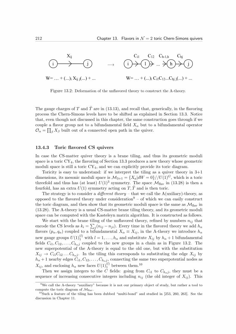
212 Chapter 13. Flavors in N = 2 toric Chern-Simons quivers
−→
Figure 13.2: Deformation of the unflavored theory to construct the A-theory.
The gauge charges of T and T are in (13.13), and recall that, generically, in the flavoringprocess the Chern-Simons levels have to be shifted as explained in Section 13.3. Noticethat, even though not discussed in this chapter, the same construction goes through if wecouple a flavor group not to a bifundamental field Xα but to a bifundamental operatorOα =
∏
β Xβ built out of a connected open path in the quiver.
13.4.3 Toric flavored CS quivers
In case the CS-matter quiver theory is a brane tiling, and thus its geometric modulispace is a toric CY4, the flavoring of Section 13.3 produces a new theory whose geometricmoduli space is still a toric CY4, and we can explicitly provide its toric diagram.
Toricity is easy to understand: if we interpret the tiling as a quiver theory in 3+1dimensions, its mesonic moduli space isM3+1 = Xa|dW = 0//U(1)G, which is a toricthreefold and thus has (at least) U(1)3 symmetry. The space Mflav in (13.28) is then afourfold, has an extra U(1) symmetry acting on T, T and is then toric.
The strategy is to consider a different theory – that we call the A(uxiliary)-theory, asopposed to the flavored theory under consideration9 – of which we can easily constructthe toric diagram, and then show that its geometric moduli space is the same asMflav in(13.28). The A-theory is a usual CS-matter brane tiling theory, and its geometric modulispace can be computed with the Kasteleyn matrix algorithm. It is constructed as follows.
We start with the brane tiling of the unflavored theory, refined by numbers nij thatencode the CS levels as ki =
∑
j(nij − nji). Every time in the flavored theory we add hαflavors (pα, qα) coupled to a bifundamental Xα ≡ Xij , in the A-theory we introduce hα
new gauge groups U(1)(l)1 with l = 1, . . . , hα and substitute Xij by hα + 1 bifundamental
fields Ci1, C12, . . . , Chαj coupled to the new groups in a chain as in Figure 13.2. Thenew superpotential of the A-theory is equal to the old one, but with the substitutionXij → Ci1C12 . . . Chαj . In the tiling this corresponds to substituting the edge Xij byhα +1 nearby edges Ci1, C12, . . . , Chαj , connecting the same two superpotential nodes as
Xij , and enclosing hα new faces U(1)(l)1 between them.10
Then we assign integers to the C fields: going from Ci1 to Chαj , they must be asequence of increasing consecutive integers including nij (the old integer of Xij). This
9We call the A-theory “auxiliary” because it is not our primary object of study, but rather a tool tocompute the toric diagram of Mflav.
10Such a feature of the tiling has been dubbed “multi-bond” and studied in [253, 260, 263]. See thediscussion in Chapter 11.
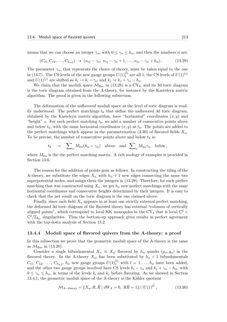
13.4. Moduli space of flavored quivers 213
means that we can choose an integer γα, with 0 ≤ γα ≤ hα, and then the numbers n are:
(Ci1, C12, . . . , Chαj) → (nij − γα, nij − γα + 1, . . . , nij − γα + hα) . (13.29)
The parameter γα, that represents the choice of theory, must be taken equal to the one
in (13.7). The CS levels of the new gauge groups U(1)(l)1 are all 1; the CS levels of U(1)(i)
and U(1)(j) are shifted as ki → ki − γα and kj → kj + γα − hα.We claim that the moduli spaceMflav in (13.28) is a CY4, and its 3d toric diagram
is the toric diagram obtained from the A-theory, for instance by the Kasteleyn matrixalgorithm. The proof is given in the following subsection.
The deformation of the unflavored moduli space at the level of toric diagram is read-ily understood. The perfect matchings tk that define the unflavored 3d toric diagram,obtained by the Kasteleyn matrix algorithm, have “horizontal” coordinates (x, y) and“height” z. For each perfect matching tk, we add a number of consecutive points aboveand below tk, with the same horizontal coordinates (x, y) as tk. The points are added tothe perfect matchings which appear in the parametrization (3.30) of flavored fields Xα.To be precise, the number of consecutive points above and below tk is:
tk →∑
αMkα(hα − γα) above and
∑
αMkαγα below ,
where Mkα is the the perfect matching matrix. A rich zoology of examples is provided inSection 13.6.
The reason for the addition of points goes as follows. In constructing the tiling of theA-theory, we substitute the edges Xα with hα + 1 new edges connecting the same twosuperpotential nodes, and assign them the integers in (13.29). Therefore, for each perfectmatching that was constructed using Xα, we get hα new perfect matchings with the samehorizontal coordinates and consecutive heights determined by their integers. It is easy tocheck that the net result on the toric diagram is the one claimed above.
Finally, since each field Xa appears in at least one strictly external perfect matching,the deformed 3d toric diagram of the flavored theory has external “columns of verticallyaligned points”, which correspond to local KK monopoles in the CY4 that is local C2 ×C2/Zhα singularities. Thus the bottom-up approach gives results in perfect agreement
with the top-down analysis of Section 13.2.
13.4.4 Moduli space of flavored quivers from the A-theory: a proof
In this subsection we prove that the geometric moduli space of the A-theory is the sameasMflav in (13.28).
Consider a single bifundamental Xα ≡ Xij flavored by hα quarks (pα, qα) in theflavored theory. In the A-theory Xij has been substituted by hα + 1 bifundamentals
Ci1, C12, . . . , Chαj , hα new gauge groups U(1)(l)1 with l = 1, . . . , hα have been added,
and the other two gauge groups involved have CS levels ki − γα and kj + γα − hα, with0 ≤ γα ≤ hα, in terms of the levels ki and kj before flavoring. As we showed in Section13.4.1, the geometric moduli space of the A-theory is the Kahler quotient
MA−theory = Xa, R, R | dWA = 0, RR = 1//U(1)G , (13.30)
214 Chapter 13. Flavors in N = 2 toric Chern-Simons quivers
where R, R are the monopoles in the A-theory, WA its superpotential and G = G+ hα isthe total number of gauge groups.
The only fields charged under the hα new groups U(1)(l)1 are Ci1, C12, . . . , Chαj , R and
R. Their charges, including U(1)ki−γα and U(1)kj+γα−hα , are:
Ci1 C12 . . . Chα−1,hα Chαj R R
U(1)ki−γα 1 0 . . . 0 0 ki − γα −ki + γα
U(1)(1)1 −1 1 0 0 1 −1
U(1)(2)1 0 −1 0 0 1 −1
......
......
......
...
U(1)(hα−1)1 0 0 1 0 1 −1
U(1)(hα)1 0 0 −1 1 1 −1
U(1)kj+γα−hα 0 0 . . . 0 −1 kj + γα − hα −kj − γα + hα
Let us perform the Kahler quotient by the complexified gauge group∏hαl=1 U(1)
(l)1 only:
it is done by introducing gauge invariants and relations between them. The independentgauge invariants are:
T ≡ R (Ci1)hα(C12)
hα−1 . . . (Chα−1,hα)1 RR = 1
T ≡ R (C12)1(C23)
2 . . . (Chαj)hα Xij ≡ Ci1C12 . . . Chαj ,
(13.31)
where we dubbed one of them as the old field Xij . The only relation is
T T = (Xij)hα . (13.32)
We see that, after quotienting, the new monopole operators are T , T and obey a “quan-tum” F-term relation. The charges of Xij , T , T under the remaining two groups are:
Xij T T
U(1)ki−γα 1 ki − γα + hα −ki + γα
U(1)kj+γα−hα −1 kj + γα − hα −kj − γα
We want to compare these charges with those in the flavored theory. When the flavoredtheory is being flavored by hα quarks, its CS levels have to be shifted by δkl =
(hα2 −
γα)gl[Xij ] (13.7), where γα is a choice of theory. Plugging into (13.13) we get:
gl[T ] = kl + (hα − γα) gl[Xij ] gl[T ] = −kl + γα gl[Xij ] . (13.33)
This precisely agrees with the table above if we identify the choice of 0 ≤ γα ≤ hα between
the flavored and A-theory. So the quotient by∏hαl=1 U(1)
(l)1 gives the A-theory monopoles
the same quantum charges as in the flavored theory.11
Let us now consider the classical F-term relations. In the A-theory, the F-terms areof two sorts: differentiating WA by a field which is not Ci1, . . . , Chαj we get the same
11The CS levels are different in the flavored and A-theory, but this does not matter. What matters forthe moduli space are the charges of chiral fields.
13.5. Back to geometry: real and complex masses 215
equation as in the flavored theory, but with Xij → Ci1 . . . Chαj ; differentiating WA byone of Ci1, . . . , Chαj we get the same equation as in the flavored theory, but multipliedby the other C fields:
(∏
C)(flavored theory relation) = 0 . (13.34)
As long as no more than one of the C fields vanishes, we exactly reproduce the sameF-terms as in the flavored theory. When more than one C field vanishes, all equationsbecome trivial and the A-theory could develop a branch which is not contained in thegeometric moduli space of the flavored theory. However, the geometric moduli spaceof the A-theory (which is the CY4) is the one where the F-terms are solved by theparametrization Xα =
∏
k tMkαk , thus if the flavored theory relations are satisfied at
C 6= 0, they are satisfied also at C = 0.We have thus shown that:
MA−theory = XAa | dWA = 0//U(1)G−2 =
= XAa , R, R | dWA = 0, RR = 1//U(1)G =
= XFa , T, T | dWflav = 0, T T =
∏
Xhαα //U(1)G =Mflav .
(13.35)
The argument is straightforwardly generalized to the case that we flavor multiple fieldsXα, each with its own hα quarks. This concludes the proof.
Let us conclude with a remark. Suppose that the theory before flavoring has someglobal Abelian symmetry, under which Xij has charge Q. Then also the A-theory hassuch a symmetry, if we assign charges Q/(hα+1) to Ci1, . . . , Chαj . It is easy to compute
that, after modding out by∏
l U(1)(l)1 , both T and T have charge hαQ/2. This reproduces
the quantum formulæ (13.12) and (13.14).
13.5 Back to geometry: real and complex masses
Each non-compact toric divisor of a toric CY3 is a strictly external point of its 2d toricdiagram. In the field theory it corresponds to a set of fields Xηη=1,...,Q (with the sameglobal charges), where Q is determined by (13.1): the equation Xη = 0, for any of the Qfields, defines the divisor as a submanifold of the mesonic moduli space. Placing a stack ofh D6-branes on the divisor introduces h flavors coupled to one of the fields Xη via thesuperpotential δW = pXηq. This follows from the fact that the modes from 2-6 stringsdescribed by (p, q) become massless when some D2-branes are on top of the D6-branes.Moreover the D6-branes carry U(h) gauge fields, which by the AdS/CFT map give riseto U(h) global symmetry in the boundary theory.
There are Q fields such that the equation Xη = 0 describes the same irreducible divi-sor. The reason is that the radial section of the divisor can have non-trivial fundamentalgroup (in the toric case π1(S
3/ZQ) = ZQ); therefore a flat connection can be specifiedas boundary condition on the D6 worldvolume, distinguishing which of the Q fields itis coupled to. The connection is then flat everywhere but at the tip, where its flux canaffect the shift of CS levels via (13.3). Indeed, flavoring different fields in the set Xηimplies shifting different CS levels (13.6). Clearly we can pile up D6-branes with differentflat connection.

216 Chapter 13. Flavors in N = 2 toric Chern-Simons quivers
The converse is not true: a generic field Xa corresponds – via the equation Xa = 0 –to a collection of pairwise intersecting toric divisors, rather than to a single irreducibledivisor. More precisely, each field is part of a set Xη1,...,Q which corresponds to acollection of consecutive strictly external points along the perimeter of the toric diagram.The number Q of fields in the set is still given by the formula in footnote 4, but takingthe cross product between two non-consecutive legs (in the (p, q)-web) that enclose thesequence of points [299]. Flavoring one of the fields Xη via δW = pXηq is accomplishedby placing a stack of D6-branes on the collection of intersecting divisors, described byXη = 0. The map is easily worked out with perfect matchings and the Kasteleyn matrixalgorithm; we gave an example in Section 3.5.4.
All these statements translate to M-theory. A stack of h D6-branes on the fibered CY3
uplift to a CY4 with h KK monopoles, which locally have complex structure C2×C
2/Zhand the geometry of a multi-Taub-NUT. The equation Xα = 0 describes the locationof the core of the multi-Taub-NUT. Such a singularity in M-theory carries SU(h) gaugefields, while the extra U(1) comes from the KK reduction of the bulk potential C3. Infact the geometry of h coincident KK monopoles is
ds2KK = U d~x · d~x+1
U(dθ +Aω)
2 with U =1
|~x| +1
λ2, (13.36)
where ~x ∈ R3, U is a harmonic function on R
3, Aω = ~ω · d~x is a U(1) connection on R3
such that dU = ∗3 dAω, θ has period 4π/h and λ is the asymptotic radius of the circle.For h = 1 the metric is smooth, otherwise it has an Ah−1 singularity. The 2-form
B = dΛ = d
[ |~x||~x|+ λ2
(dθ +Aω
)]
(13.37)
is closed, anti-self-dual, regular and integrable. Thus a local KK reduction C3 = A ∧ Bgives an extra U(1) gauge field propagating around the core of the multi-Taub-NUT.
The flat boundary condition for the connection on the D6-branes uplifts to a flatboundary condition for C3 (and possibly the gauge fields at the singularity). However,since in type IIA the connection is not flat at the tip and its flux can affect the CSlevels which ultimately determine the fibration of the CY3 along R, in M-theory differentboundary conditions can uplift to different geometries. An example will be given insubsection 13.6.3.
13.5.1 Real masses and partial resolutions
We can introduce real masses for chiral fields with the term∫
d4θ Z†e2imθθZ . (13.38)
As in Section 13.3, we can think of the real mass as a VEV for a background scalar σF ,in the N = 2 vector multiplet of U(h). In this way we give opposite mass to the flavorsp and q. The VEV of σF corresponds to the position of the D6-branes along the real lineR transverse to the CY3. When the D6-branes at r0 are displaced from the D2-branesat the tip, the flavors can be integrated out at low energy. We showed in (13.3) that
13.5. Back to geometry: real and complex masses 217
opposite signs for σF affect the CS levels, consistently with the field theory discussion inSection 13.3.
Real masses, like Fayet-Iliopoulos parameters, do not affect the superpotential [217].Uplifting to M-theory, real masses do not affect the complex structure of the CY4 butrather its Kahler parameters: they correspond to blowing up a 2-cycle. In simple exam-ples, integrating out a flavor pair corresponds to removing a single strictly external pointfrom the 3d toric diagram: the local C2 ×C
2/Zh singularity manifests itself as a columnof h + 1 external points, and integrating out a quark pair with negative (positive) 〈σF 〉corresponds to a partial resolution of the upmost (lowest) point in the column. Only inthis limit of infinite mass/resolution parameter, the effective complex structure changes,as the removal of the point in the toric diagram shows. In more complicated situations,the partial resolution corresponding to giving infinite real mass to a flavor pair couldcorrespond to removing more than one point: the precise map is via perfect matchings,as analyzed in Section 13.4.2.
13.5.2 Complex masses
Complex masses for the flavors can correspond to geometric deformations of the D6-brane embeddings, but not always. Suppose we want to flavor a bifundamental operatorOα =
∏
β Xβ , made of an open chain of bifundamental fields. We can proceed in thefollowing way: we flavor each field Xβ separately, and then introduce complex masses foreach chiral pair:
W =W0 +n∑
β=1
pβXβqβ +n−1∑
β=1
mβ pβ+1qβ . (13.39)
After integrating out the massive flavors, we get
W =W0 +(−1)n−1
∏
βmβp1(∏
βXβ
)qn ≡W0 + pαOαqα , (13.40)
with suitable redefinition of fields. Since fermions in vector-like representations do notcontribute to the monopole charges, the quantum F-term relation is unmodified:
T T =∏
α(Xα)
hα = (Oα)hα . (13.41)
Therefore the two theories where we flavor Oα or each Xβ separately have the samegeometric moduli space, and can only differ in their Higgs branches.
The complex masses mβ do not correspond to deformations of the D6-brane embed-dings. In fact we can probe the embedding with D2-branes: the quarks become masslesson⋃
βXβ = 0, which does not depend on mβ . Such masses correspond to VEVs forhigher dimensional fields localized at the intersection of the D6-branes, which do notchange the embedding.
This leads to the following natural generalization. Consider starting with a conicalCY3, not necessarily toric, and its dual quiver theory defined by D3-branes probing it.We can always include RR fluxes and fiber it along R, that is add N = 2 Chern-Simonsterms in field theory (the geometry then uplifts to a CY4 in M-theory). Then consider a
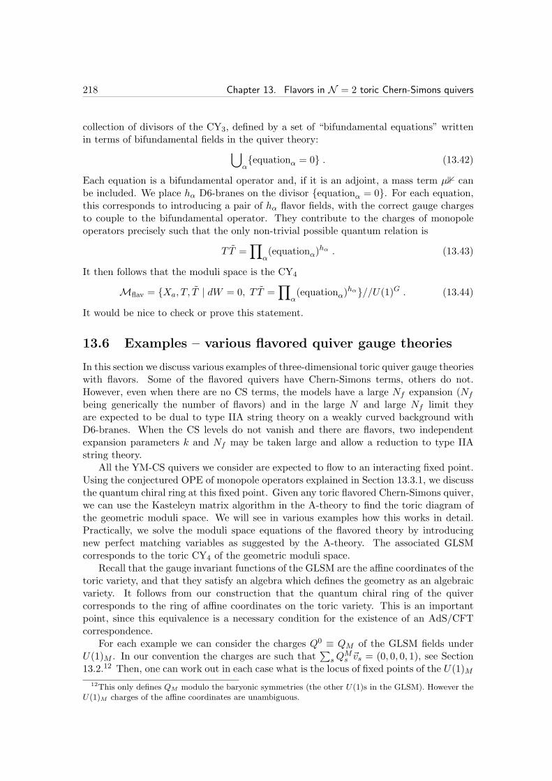
218 Chapter 13. Flavors in N = 2 toric Chern-Simons quivers
collection of divisors of the CY3, defined by a set of “bifundamental equations” writtenin terms of bifundamental fields in the quiver theory:
⋃
αequationα = 0 . (13.42)
Each equation is a bifundamental operator and, if it is an adjoint, a mass term µ1 canbe included. We place hα D6-branes on the divisor equationα = 0. For each equation,this corresponds to introducing a pair of hα flavor fields, with the correct gauge chargesto couple to the bifundamental operator. They contribute to the charges of monopoleoperators precisely such that the only non-trivial possible quantum relation is
T T =∏
α(equationα)
hα . (13.43)
It then follows that the moduli space is the CY4
Mflav = Xa, T, T | dW = 0, T T =∏
α(equationα)
hα//U(1)G . (13.44)
It would be nice to check or prove this statement.
13.6 Examples – various flavored quiver gauge theories
In this section we discuss various examples of three-dimensional toric quiver gauge theorieswith flavors. Some of the flavored quivers have Chern-Simons terms, others do not.However, even when there are no CS terms, the models have a large Nf expansion (Nf
being generically the number of flavors) and in the large N and large Nf limit theyare expected to be dual to type IIA string theory on a weakly curved background withD6-branes. When the CS levels do not vanish and there are flavors, two independentexpansion parameters k and Nf may be taken large and allow a reduction to type IIAstring theory.
All the YM-CS quivers we consider are expected to flow to an interacting fixed point.Using the conjectured OPE of monopole operators explained in Section 13.3.1, we discussthe quantum chiral ring at this fixed point. Given any toric flavored Chern-Simons quiver,we can use the Kasteleyn matrix algorithm in the A-theory to find the toric diagram ofthe geometric moduli space. We will see in various examples how this works in detail.Practically, we solve the moduli space equations of the flavored theory by introducingnew perfect matching variables as suggested by the A-theory. The associated GLSMcorresponds to the toric CY4 of the geometric moduli space.
Recall that the gauge invariant functions of the GLSM are the affine coordinates of thetoric variety, and that they satisfy an algebra which defines the geometry as an algebraicvariety. It follows from our construction that the quantum chiral ring of the quivercorresponds to the ring of affine coordinates on the toric variety. This is an importantpoint, since this equivalence is a necessary condition for the existence of an AdS/CFTcorrespondence.
For each example we can consider the charges Q0 ≡ QM of the GLSM fields underU(1)M . In our convention the charges are such that
∑
sQMs ~vs = (0, 0, 0, 1), see Section
13.2.12 Then, one can work out in each case what is the locus of fixed points of the U(1)M12This only defines QM modulo the baryonic symmetries (the other U(1)s in the GLSM). However the
U(1)M charges of the affine coordinates are unambiguous.
13.6. Examples – various flavored quiver gauge theories 219
action, and to which divisors it corresponds to in the type IIA reduction, making the linkwith the top-down approach of Section 13.2.
Let us fix the notation. The perfect matching variables ti of the unflavored quiverare denoted az, bz, cz, · · · , with z the vertical coordinate of the corresponding point in thetoric diagram. The toric diagram of the flavored theory is obtained by adding columnsof points above and below some of the original points, as explained in Section 13.4.2. Byan SL(4,Z) transformation, we can always set the base of three of the columns of pointsto z = 0. We will always choose such a convenient frame. Although we consider quiverswith Abelian gauge groups only, we nevertheless write the non-Abelian superpotentials,in order to make the link with well-known quivers more explicit.
13.6.1 Flavoring the C3 quiver
Our first example is the flavoring of N = 8 SYM, the low energy field theory on a D2-brane on flat C
3 × R. The quiver is simply that of N = 4 SYM in 3+1 dimensions. InN = 2 notation, we have a single vector superfield and three adjoint chiral superfieldsΦ1, Φ2, Φ3, with superpotential W = Φ1[Φ2,Φ3].
We can add one, two or three flavor groups by coupling flavors to the appropriatechiral superfields, as shown in Figure 13.3. We denote by pi and qi the fundamental andantifundamental fields in the i-th flavor group coupled to the field Φi. The flavoring of a Φicorresponds to introducing D6-branes at zi = 0, x9 = 0, and D2/D6-brane intersectionsinduce the superpotential
W = Φ1[Φ2,Φ3] +
h1∑
i=1
p1,iΦ1q1,i +
h2∑
j=1
p2,jΦ2q2,j +
h3∑
l=1
p3,lΦ3q3,l . (13.45)
In the general case, the flavor group is GF = U(h1)×U(h2)×U(h3)/U(1). The charges ofthe fields under the various gauge and global symmetries are summarized in the followingtable:
Φi p1 q1 p2 q2 p3 q3 T T
U(1) 0 −1 1 −1 1 −1 1 0 0
U(h1) (1) (h1) (h1) (1) (1) (1) (1) (1) (1)
U(h2) (1) (1) (1) (h2) (h2) (1) (1) (1) (1)
U(h3) (1) (1) (1) (1) (1) (h3) (h3) (1) (1)
(13.46)
In this simple case, flavor groups are non-chirally coupled and so the monopole operatorsT , T do not acquire any gauge charge. Nevertheless, they do acquire some R-charge,
R(T ) = R(T ) =1
2
(h1R(Φ1) + h2R(Φ2) + h2R(Φ2)
). (13.47)
The quantum holomorphic relation (13.15) is
T T = Φh11 Φh22 Φh33 . (13.48)
It describes an affine variety whose affine coordinates are the five gauge invariant operatorsT , T and Φi (in the case of a U(N) gauge group one should consider the eigenvalues). Letus discuss a few particular cases related to known models in the literature [253, 263, 290].

220 Chapter 13. Flavors in N = 2 toric Chern-Simons quivers
(a) Quiver withone flavor group.
(b) Quiver with two flavorgroups.
(c) Quiver with three flavorgroups.
Figure 13.3: Quivers for flavored SQED. Circles are gauge groups, squares are flavor groups.Colored arrows indicate bifundamental fields coupled to flavors via a superpotential term.
(a) C4 (b) C × C (c) D3
Figure 13.4: Toric diagrams corresponding to some flavors for the C3 quiver.
• In the case h2 = h3 = 0, The chiral ring relation is
T T = Φh11 , (13.49)
and the geometric branch of the moduli space is C2 × C2/Zh1 . For h1 = 1 we have
C4, see Figure 13.4(a). This model is related to the dual ABJM model of [253, 263].
We discuss it in a bit more details in Section 13.6.1.
• For h1 = h2 = 1, h3 = 0, we have C × C (C the conifold), see Fig. 13.4(b). TheA-theory for this model is the so-called Phase III of C× C discussed in [263].
• For h1 = 2, h2 = 1, h3 = 0, we have C times the suspended pinch point (SPP).This was also noticed in [290]. In general, for h1 = a, h2 = b, the geometry isC× C(Laba).
• For h1 = h2 = h3 = 1, the geometry is D3, see Fig. 13.4(c) . The A-theory for thismodel is the Phase III of D3 discussed in [263].
When some hi > 1, these geometries have non-isolated singularities. Remark that wehave considered the most general toric flavoring of the C
3 quiver. The GLSM for the

13.6. Examples – various flavored quiver gauge theories 221
Figure 13.5: Toric diagrams of C2 × C2/Zh, for h = 3.
strictly external points is
t1 t2 t3 t4 t5 t6U(1)B1 h2 −h1 0 −h2 h1 0U(1)B2 0 h3 −h2 0 −h3 h2U(1)B3 −h3 0 h1 h3 0 −h1
(13.50)
This GLSM does not encode various orbifold identifications which might in general arise:for a full description of the geometry one should consider the full GLSM, encoding all therelations in the toric diagram, with h1 + h2 + h3 + 3 homogeneous coordinates.
Flavoring Φ1: the dual ABJM geometry
Let us discuss a bit more in detail the case C2 × C
2/Zh. This geometry has the toricdiagram shown in Figure 13.5,
a0 = (0, 0, 0), · · · , ah = (0, 0, h), b0 = (0, 1, 0), c0 = (1, 0, 0) (13.51)
There are h+ 3 homogeneous coordinates, and GLSM
a0 b0 c0 a1 a2 a3 · · · ah−1 ahU(1)B1 1 0 0 −2 1 0 · · · 0 0U(1)B2 0 0 0 1 −2 1 · · · 0 0U(1)B3 0 0 0 0 1 −2 · · · 0 0...
. . .
U(1)Bh−10 0 0 0 0 0 · · · −2 1
U(1)M 1 0 0 −1 0 0 · · · 0 0
(13.52)
222 Chapter 13. Flavors in N = 2 toric Chern-Simons quivers
The five affine coordinates are
x1 = Φ1 = a0a1 . . . ah−1ah , x2 = T = ah0ah−11 . . . a2h−2ah−1 ,
x3 = T = a1a22 . . . a
h−1h−1a
hh , x4 = Φ2 = b0 , x5 = Φ3 = c0 ,
(13.53)and of course they satisfy
x2x3 = xh1 . (13.54)
Also, the QM charges of (x1, · · · , x5) are (0, 1,−1, 0, 0), so that U(1)M has fixed pointsat x2 = x3 = 0. Gauging U(1)M , we get the type IIA geometry, which is C3 spanned by(z1, z2, z3) = (x1, x4, x5) since the gauge invariant coordinate x2x3 can be eliminated by(13.54). The locus of fixed points of U(1)M in the CY4 descends to the divisor x1 = 0 inC3, where we must have a stack of h D6-branes. This was the argument of section 13.2,
which motivates the field theory we presented.Note that the same geometry is obtained as the moduli space of the so-called dual
ABJM model of [253], at CS level h. This model was also studied in [263, 307, 272], andsome puzzles were found. At h = 1, the dual ABJM model corresponds to the A-theoryfor our flavored theory with a single flavor. For h flavors, our A-theory is a tiling withan (h+ 1)-ple bond. It would be interesting to compare in more details our proposal tothe one of [253].
For some specific values of the superpotential couplings, the supersymmetry of ourflavored quiver gets enhanced to N = 4, since the geometry C
2×C2/Zh is hyper-Kahler.
Indeed, our setup is a N = 2 version of the setup considered in [207].
13.6.2 Flavoring the conifold quiver
Consider the quiver of the ABJM theory, equal to the Klebanov-Witten (KW) quiverfor D-branes on the conifold C. It has two nodes, four bifundamental fields, A1, A2, B1,B2, and superpotential W = A1B1A2B2 −A1B2A2B1. There are four points in the toricdiagram of C4/Zk, corresponding to the four perfect matchings in the brane tiling of theconifold theory and to the bifundamental fields: because the F-term relations are trivialin the Abelian theory, we can write (with abuse of notation)
ak = A1 = (0, 0, k) , b0 = B1 = (0, 1, 0) ,
c0 = A2 = (1, 1, 0) , d0 = B2 = (1, 0, 0) .(13.55)
We then consider the toric diagram obtained by adding four columns of points of heightsha, hb, hc, hd above the four base points (any other choice of adding the points above orbelow, is SL(4,Z) equivalent to this up to a change in k):
ak+i = (0, 0, k + i) , bj = (0, 1, j) , cl = (1, 1, l) , dm = (1, 0,m) , (13.56)
where i = 0, . . . , ha, j = 0, . . . , hb, l = 0, . . . , hc, m = 0, . . . , hd. See Figure 13.6(b).This toric geometry corresponds to a generic flavoring of the ABJM theory at level
k, with flavor group GF = U(ha)×U(hb)×U(hc)×U(hd)/U(1). The quiver is shown inFigure 13.6(a), and the superpotential is
W = A1B1A2B2 −A1B2A2B1+
+
ha∑
i=1
p1,iA1q1,i +
hb∑
j=1
p2,jB1q2,j +
hc∑
l=1
p3,lA2q3,l +
hd∑
r=1
p4,rB2q4,r .(13.57)
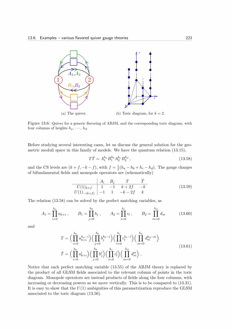
13.6. Examples – various flavored quiver gauge theories 223
(a) The quiver. (b) Toric diagram, for k = 2.
Figure 13.6: Quiver for a generic flavoring of ABJM, and the corresponding toric diagram, withfour columns of heights ha, · · · , hd.
Before studying several interesting cases, let us discuss the general solution for the geo-metric moduli space in this family of models. We have the quantum relation (13.15),
T T = Aha1 Bhb1 A
hc2 B
hd2 , (13.58)
and the CS levels are (k+ f,−k− f), with f = 12(ha − hb + hc − hd). The gauge charges
of bifundamental fields and monopole operators are (schematically)
Ai Bj T T
U(1)k+f 1 −1 k + 2f −kU(1)−(k+f) −1 1 −k − 2f k
(13.59)
The relation (13.58) can be solved by the perfect matching variables, as
A1 =
ha∏
i=0
ak+i , B1 =
hb∏
j=0
bj , A2 =
hc∏
l=0
cl , B2 =
hd∏
m=0
dm (13.60)
and
T =( ha∏
i=0
aha−ik+i
)( hb∏
j=0
bhb−jj
)( hc∏
l=0
chc−ll
)( hd∏
m=0
dhd−mm
)
T =( ha∏
i=0
aik+i
)( hb∏
j=0
bjj
)( hc∏
l=0
cll
)( hd∏
m=0
dmm
)
,
(13.61)
Notice that each perfect matching variable (13.55) of the ABJM theory is replaced bythe product of all GLSM fields associated to the relevant column of points in the toricdiagram. Monopole operators are instead products of fields along the four columns, withincreasing or decreasing powers as we move vertically. This is to be compared to (13.31).It is easy to show that the U(1) ambiguities of this parametrization reproduce the GLSMassociated to the toric diagram (13.56).
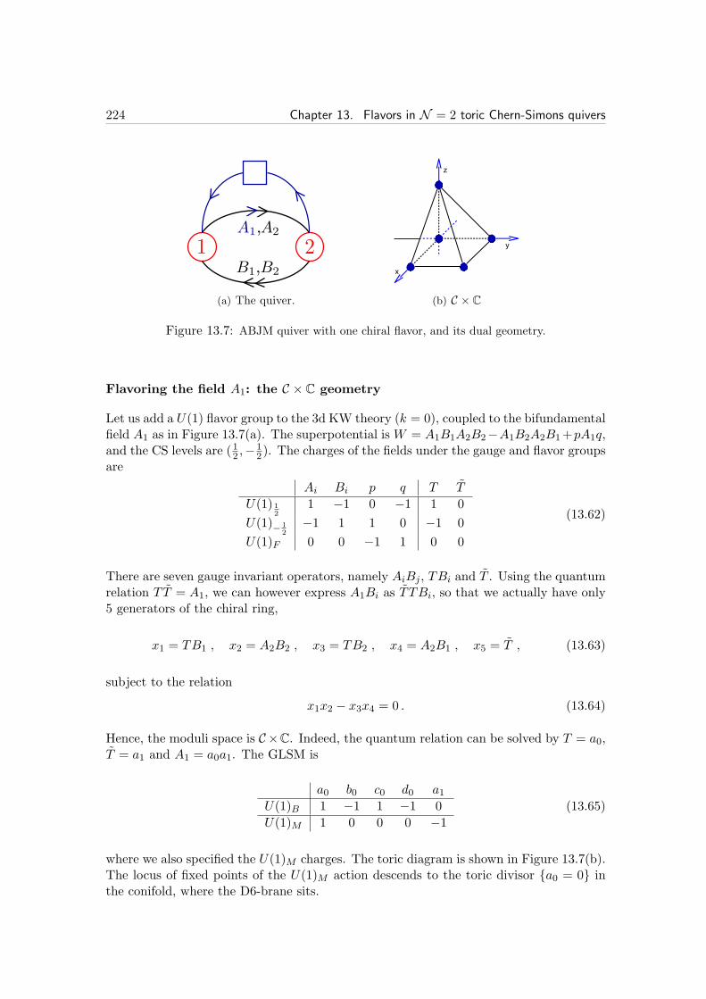
224 Chapter 13. Flavors in N = 2 toric Chern-Simons quivers
(a) The quiver. (b) C × C
Figure 13.7: ABJM quiver with one chiral flavor, and its dual geometry.
Flavoring the field A1: the C × C geometry
Let us add a U(1) flavor group to the 3d KW theory (k = 0), coupled to the bifundamentalfield A1 as in Figure 13.7(a). The superpotential isW = A1B1A2B2−A1B2A2B1+pA1q,and the CS levels are (12 ,−1
2). The charges of the fields under the gauge and flavor groupsare
Ai Bi p q T T
U(1) 12
1 −1 0 −1 1 0
U(1)− 12−1 1 1 0 −1 0
U(1)F 0 0 −1 1 0 0
(13.62)
There are seven gauge invariant operators, namely AiBj , TBi and T . Using the quantumrelation T T = A1, we can however express A1Bi as T TBi, so that we actually have only5 generators of the chiral ring,
x1 = TB1 , x2 = A2B2 , x3 = TB2 , x4 = A2B1 , x5 = T , (13.63)
subject to the relation
x1x2 − x3x4 = 0 . (13.64)
Hence, the moduli space is C ×C. Indeed, the quantum relation can be solved by T = a0,T = a1 and A1 = a0a1. The GLSM is
a0 b0 c0 d0 a1U(1)B 1 −1 1 −1 0
U(1)M 1 0 0 0 −1(13.65)
where we also specified the U(1)M charges. The toric diagram is shown in Figure 13.7(b).The locus of fixed points of the U(1)M action descends to the toric divisor a0 = 0 inthe conifold, where the D6-brane sits.
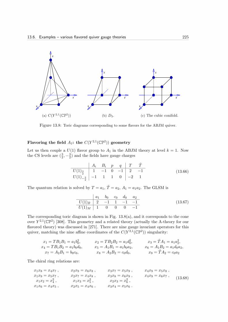
13.6. Examples – various flavored quiver gauge theories 225
(a) C(Y 2,1(CP2)) (b) D3. (c) The cubic conifold.
Figure 13.8: Toric diagrams corresponding to some flavors for the ABJM quiver.
Flavoring the field A1: the C(Y 2,1(CP2)) geometry
Let us then couple a U(1) flavor group to A1 in the ABJM theory at level k = 1. Nowthe CS levels are (32 ,−3
2) and the fields have gauge charges
Ai Bi p q T T
U(1) 32
1 −1 0 −1 2 −1U(1)− 3
2−1 1 1 0 −2 1
(13.66)
The quantum relation is solved by T = a1, T = a2, A1 = a1a2. The GLSM is
a1 b0 c0 d0 a2U(1)B 2 −1 1 −1 −1U(1)M 1 0 0 0 −1
(13.67)
The corresponding toric diagram is shown in Fig. 13.8(a), and it corresponds to the coneover Y 2,1(CP2) [308]. This geometry and a related theory (actually the A-theory for ourflavored theory) was discussed in [271]. There are nine gauge invariant operators for thisquiver, matching the nine affine coordinates of the C(Y 2,1(CP2)) singularity:
x1 = TB1B1 = a1b20, x2 = TB2B2 = a1d
20, x3 = TA1 = a1a
22,
x4 = TB1B2 = a1b0d0, x5 = A1B1 = a1b0a2, x6 = A1B2 = a1d0a2,
x7 = A2B1 = b0c0, x8 = A2B2 = c0d0, x9 = TA2 = c0a2
The chiral ring relations are:
x1x8 = x4x7 , x2x9 = x6x8 , x3x7 = x5x9 , x4x9 = x5x8 ,x1x9 = x5x7 , x2x7 = x4x8 , x3x8 = x6x9 , x4x9 = x6x7 ,x1x2 = x24 , x1x3 = x25 , x2x3 = x26 ,x1x6 = x4x5 , x2x5 = x4x6 , x3x4 = x5x6 .
(13.68)

226 Chapter 13. Flavors in N = 2 toric Chern-Simons quivers
(a) ABJM quiver with two chiral flavor groups. (b) C(Q1,1,1).
Figure 13.9: ABJM quiver with two chiral flavor groups, and a dual geometry.
Flavoring the fields A1 and A2: the C(Q1,1,1) geometry
Consider the conifold quiver with two U(1) flavor groups coupled to A1 and A2 respec-tively, as in Fig. 13.9(a). The superpotential is
W = A1B1A2B2 −A1B2A2B1 + p1A1q1 + p2A2q2 , (13.69)
and we choose vanishing CS levels. In the toric diagram, this corresponds to adding onepoint below a0 and one point above c0, see Fig. 13.9(b). The gauge charges of the fieldsand monopole operators are
Ai Bi pi qi T T
U(1)0 1 −1 0 −1 1 1U(1)0 −1 1 1 0 −1 −1
(13.70)
The monopole operators satisfy the relation
T T = A1A2 . (13.71)
We can solve it by introducing two new perfect matching variables a−1 and c1:
A1 = a−1a0, B1 = b0, T = a−1c0,
A2 = c0c1, B2 = d0, T = a0c1.(13.72)
The associated GLSM is a minimal presentation of the one for the real cone over Q1,1,1:
a0 b0 c0 d0 a−1 c1U(1)B1 1 −1 1 −1 0 0U(1)B2 1 0 1 0 −1 −1U(1)M 0 0 1 0 0 −1
(13.73)
The gauge invariant operators generating the chiral ring are:
x1 = A1B1 = a−1a0b0, x2 = A2B2 = c0c1d0, x3 = A2B1 = b0c0c1,
x4 = A1B2 = a−1a0d0, x5 = TB1 = a0b0c1, x6 = TB2 = a0c1d0,x7 = TB1 = a−1b0c0, x8 = TB2 = a−1c0d0.

13.6. Examples – various flavored quiver gauge theories 227
They of course correspond to the affine coordinates on C(Q1,1,1), whose algebra is
x1x2 − x3x4 = 0 , x1x2 − x5x8 = 0 , x1x2 − x6x7 = 0 ,x1x3 − x5x7 = 0 , x1x6 − x4x5 = 0 , x1x8 − x4x7 = 0 ,x2x4 − x6x8 = 0 , x2x5 − x3x6 = 0 , x2x7 − x3x8 = 0 .
(13.74)
Remark that the affine coordinates have U(1)M charges
x1 x2 x3 x4 x5 x6 x7 x8U(1)M 0 0 0 0 −1 −1 1 1
(13.75)
so the U(1)M fixed point locus is at x5 = x6 = x7 = x8 = 0, x1x2 = x3x4 = x1x3 =x2x4 = 0. This locus of fixed points has two branches:
1) x1 = x4 = 0 , x5 = x6 = x7 = x8 = 0 , ∀x2, x3 ⇐⇒ a0 = a−1 = 0
2) x2 = x3 = 0 , x5 = x6 = x7 = x8 = 0 , ∀x1, x4 ⇐⇒ c0 = c1 = 0 .(13.76)
It is easy to see that they descend to the toric divisors a0 = 0 and c0 = 0 in theconifold C. The D6-branes wrapping these divisors provide us with the chiral flavors inthe quiver field theory.
Another quiver for the low energy field theory on M2-branes on C(Q1,1,1) was proposedin [259], and further studied in [262]. The quiver of [259], which has two double-bonds,is precisely the A-theory of our chirally flavored conifold theory.
Flavoring the fields A1 and B1: the D3 geometry
Let us now couple a U(1) flavor group to A1 and a U(1) flavor group to B1, with δW =p1A1q1+ p1B1q1 and vanishing CS levels. In this case there is no induced gauge charge forthe monopole operators, because there are as many incoming as outgoing arrows in eachgauge group. We have the quantum relation T T = A1B1, which is solved by A1 = a0a1,B1 = b0b1, T = a0b0 and T = a1b1. The associated GLSM is
a0 b0 c0 d0 a1 b1U(1)B1 1 −1 1 −1 0 0U(1)B2 1 −1 0 0 −1 1
U(1)M 1 0 0 0 −1 0
(13.77)
The toric diagram, shown in Fig. 13.8(b), is the one of the D3 geometry. The generatorsof the chiral ring are
x1 = T , x2 = A2B2 , x3 = T , x4 = A1B2 , x5 = A2B1 . (13.78)
As expected, they satisfy the defining equation of the D3 singularity:
x1x2x3 − x4x5 = 0 . (13.79)
The locus of fixed points of U(1)M has two branches which descend to the two divisorsa0 = 0 and b0 = 0 in the conifold.

228 Chapter 13. Flavors in N = 2 toric Chern-Simons quivers
(a) The A1 quiver. (b) C× C.
Figure 13.10: Quiver of the modified C× C2/Z2 model (CS levels (1,−1)), and moduli space.
Flavoring A1, A2, B1, B2: the cubic conifold
Consider coupling a U(1) flavor group to each bifundamental field, with vanishing CSlevels. The quantum relation is
T T = A1B1A2B2 . (13.80)
One can check that the moduli space is described by the following GLSM:
a0 b0 c0 d0 a1 b1 c1 d1U(1)B1 1 −1 1 −1 0 0 0 0U(1)B2 0 0 0 0 1 −1 1 −1U(1)B3 1 0 0 −1 −1 0 0 1U(1)B4 1 −1 0 0 −1 1 0 0
U(1)M 1 0 0 0 −1 0 0 0
(13.81)
The toric diagram is shown in Fig. 13.8(c), and we will call this geometry the cubicconifold. The gauge invariant operators are
x1 = a0b0c0d0 = T, x2 = a1b1c1d1 = T , x3 = a0b0a1b1 = A1B1,x4 = c0d0c1d1 = A2B2, x5 = a0d0a1d1 = A1B2, x6 = b0c0b1c1 = A2B1,
satisfying the equations
x1x2 − x3x4 = 0 , x1x2 − x5x6 = 0 . (13.82)
This is a complete intersection. The U(1)M charges of (x1, · · · , x6) are (1,−1, 0, 0, 0, 0).The locus of fixed point is at x1 = x2 = 0, x3x4 = x5x6 = 0, which has four branches anddescend to the four toric divisors of the conifold.
13.6.3 Flavoring the modified C× C2/Z2 theory
In this section we add flavors to the so-called modified C × C2/Z2 theory of [245]. The
quiver of the unflavored theory, Fig. 13.10(a), is the one for D-branes at a C × C2/Z2
singularity; we choose the height numbers nij equal to 1 for the bifundamental X112 and
0 otherwise, so that the two gauge groups have CS levels (1,−1). The superpotential is
W = Φ1(X112X
221 −X2
12X121)− Φ2(X
221X
112 −X1
21X212) . (13.83)

13.6. Examples – various flavored quiver gauge theories 229
(a) CS levels (0, 0). (b) One flavored bifundamental. (c) CS levels (1,−1).
Figure 13.11: The C× C2/Z2 quiver with a U(2) flavor group coupled to X1
12. Those two toricquivers are obtained by fixing the CS levels as indicated.
From the permanent of the Kasteleyn matrix,
PermK = X121X
221 +X2
12X221 x+X1
21X112 x
−1z +X112X
212 z +Φ1Φ2 y , (13.84)
we see that the perfect matchings are
a0 = X121, X
221 = (0, 0, 0), d1 = X1
12, X212 = (0, 0, 1),
b0 = X212, X
221 = (1, 0, 0), e0 = Φ1,Φ2 = (0, 1, 0),
c1 = X121, X
112 = (−1, 0, 1).
(13.85)
The 3d toric diagram, Fig. 13.10(b), is the one of C × C. The F-term equations implyX1
12X221 = X2
12X121 and Φ1 = Φ2 along the mesonic branch. They are solved by
X112 = c1 d1 , X2
12 = b0 d1 , X121 = a0 c1 , X2
21 = a0 b0 , Φ1 = Φ2 = e0 .
The face in the 3d toric diagram whose vertices are a0, c1, d1, b0 is vertical, thereforeadditional objects may appear in the type IIA background. Nevertheless, encouragedby the results of [245] where the geometric moduli space was successfully matched withC× C, we will trust the duality and add flavors to this model.
We will study three illustrative examples where two flavor pairs are added to thistheory.
U(2) flavor group coupled to X112: levels (0, 0)
We study two cases where we couple a U(2) flavor group to X112, as in Fig. 13.11(b).
Consider first the case where the CS levels vanish. The bifundamental fields and monopoleoperators of the quiver theory have gauge charges
X12 X21 Φ T T
U(1)0 1 −1 0 1 1U(1)0 −1 1 0 −1 −1
(13.86)
230 Chapter 13. Flavors in N = 2 toric Chern-Simons quivers
The gauge invariant operators in the geometric branch are Φ, X12X21, TX21, TX21.In the A-theory, this flavoring corresponds to replacing the edge X1
12 with nX112
= 1 inthe original brane tiling with a triple-bond with n = −1, 0, 1. It amounts to consideringa 3d toric diagram with the points a0, b0, c−1, c0, c1, d−1, d0, d1, e0 as in Fig. 13.11(a).We solve for the F-term relation and the quantum relation T T = X1
12 by
X112 = c−1 c0 c1 d−1 d0 d1 , X2
12 = b0 d−1 d0 d1 ,
X121 = a0 c−1 c0 c1 , X2
21 = a0 b0 , Φ1 = Φ2 = e0 ,
T = c0 c21 d0 d
21 , T = c2−1 c0 d
2−1 d0 .
(13.87)
The charges of the homogeneous coordinates of the four-fold and of the quiver theoryfields under the associated U(1)5 GLSM are
a0 b0 c1 d1 e0 c0 d0 c−1 d−1 X12 X21 Φ T T
U(1)B1 1 −1 −1 1 0 0 0 0 0 0 0 0 0 0U(1)B2 1 0 1 −1 0 −1 0 0 0 −1 1 0 −1 −1U(1)B3 1 0 0 0 0 0 −1 0 0 −1 1 0 −1 −1U(1)B4 1 0 0 0 0 −1 0 1 −1 −1 1 0 −1 −1U(1)B5 −2 0 0 1 0 0 0 0 1 2 −2 0 2 2
matching the gauge charges (13.86). The affine coordinates of the fourfold match thegauge invariant operators of the flavored quiver theory:
x1 = e0 = Φ1 = Φ2 , x2 = a0 b20 d−1 d0 d1 = X2
12X221 ,
x3 = a0 b0 c0 c21 d0 d
21 = TX2
21 , x4 = a0 c−1 c20 c
31 d0 d
21 = TX1
21 ,
x5 = a0 b0 c−1 c0 c1 d−1 d0 d1 = X112X
221 = X2
12X121 ,
x6 = a0 c2−1 c
20 c
21 d−1 d0 d1 = X1
12X121 ,
x7 = a0 b0 c2−1 c0 d
2−1 d0 = TX2
21 , x8 = a0 c3−1 c
20 c1 d
2−1 d0 = TX1
21 .
(13.88)
U(2) flavor group coupled to X112: levels (1,−1)
Consider now the case of CS levels (1,−1). The gauge charges are:
X12 X21 Φ T T
U(1)1 1 −1 0 2 0U(1)−1 −1 1 0 2 0
(13.89)
The gauge invariant operators are Φ, X12X21, T (X21)2, T .
In the A-theory, this flavoring corresponds to replacing the edge X112 with nX1
12= 1
in the original brane tiling by a triple-bond with n = 0, 1, 2. The GLSM field appearingin the 3d toric diagram, Fig. 13.11(c), are a0, b0, c0, c1, c2, d0, d1, d2, e0. We solve forthe geometric moduli space by setting
X112 = c0 c1 c2 d0 d1 d2 , X2
12 = b0 d0 d1 d2 ,
X121 = a0 c0 c1 c2 , X2
21 = a0 b0 , Φ1 = Φ2 = e0 ,
T = c1 c22 d1 d
22 , T = c20 c1 d
20 d1 .
(13.90)

13.6. Examples – various flavored quiver gauge theories 231
(a) The quiver. (b) Toric diagram when the CS levels are (1,−1).
Figure 13.12: Modified C×C2/Z2 model with two flavored bifundamentals, and dual geometry.
The charges of the homogeneous coordinates of the fourfold and of the quiver theoryfields under the U(1)5 GLSM are
a0 b0 c1 d1 e0 c0 d0 c2 d2 X12 X21 Φ T T
U(1)B1 1 −1 −1 1 0 0 0 0 0 0 0 0 0 0U(1)B2 1 0 1 −1 0 −1 0 0 0 −1 1 0 −2 0U(1)B3 1 0 0 0 0 0 −1 0 0 −1 1 0 −2 0U(1)B4 1 0 0 −2 0 0 0 0 1 −1 1 0 −2 0U(1)B5 0 0 −2 0 0 1 0 1 0 0 0 0 0 0
matching the gauge charges (13.89). The affine coordinates of the four-fold match theholomorphic gauge invariants of the flavored quiver theory:
x1 = a0 b0 c0 c1 c2 d0 d1 d2 = X112X
221 = X2
12X121 , x2 = e0 = Φ1 = Φ2 ,
x3 = a20 b20 c
20 c1 d
20 d1 = T (X2
21)2 , x4 = a0 c
20 c
21 c
22 d0 d1 d2 = X1
12X121 ,
x5 = a20 b0 c30 c
21 c2 d
20 d1 = TX1
21X221 , x6 = a0 b
20 d0 d1 d2 = X2
12X221 ,
x7 = a20 c40 c
31 c
22 d
20 d1 = T (X1
21)2 , x8 = c1 c
22 d1 d
22 = T .
U(1)2 flavor groups coupled to X112 and X1
21: levels (1,−1)Let us study a case where we couple a U(1) flavor group to X1
12 and a U(1) flavor groupto X1
21, as in Fig. 13.12(a). The quantum relation reads T T = X112X
212. We consider the
case with CS levels (1,−1): bifundamentals and monopole operators charges are
X12 X21 Φ T T
U(1)1 1 −1 0 1 −1U(1)−1 −1 1 0 −1 1
(13.91)
The gauge invariant operators are Φ, X12X21, TX21, TX12.In the A-theory, this flavoring corresponds to replacing the edge X1
12 with nX112
= 1
in the brane tiling by a double-bond with n = 0, 1, and the edge X121 with nX1
21= 0 by
another double-bond, with n = −1, 0. All the other nij vanish. This gives a 3d toricdiagram with points a−1, a0, b0, c−1, c0, c
′0, c1, d0, d1, e0, Fig. 13.12(b). This is not a
232 Chapter 13. Flavors in N = 2 toric Chern-Simons quivers
minimal presentation of the toric diagram. In particular, unlike for the other multiplic-ities, the distinction between c0 and c′0 is not needed to express the bifundamentals andmonopole operators in terms of GLSM fields solving the F-term equations. It is possibleto replace the two of them by a single field c0 (setting c0 c
′0 = c0 in the formulæ below),
getting rid of a U(1) in the GLSM. We will do that in the following. Keeping insteadall the perfect matching fields of the A-theory may be useful in the study of partialresolutions dual to real mass terms.
We solve for the geometric moduli space by setting
X112 = c−1 c0 c1 d0 d1 , X2
12 = b0 d0 d1 ,
X121 = a−1 a0 c−1 c0 c1 , X2
21 = a−1 a0 b0 , Φ1 = Φ2 = e0 ,
T = a0 c0 c21 d1 , T = a−1 c
2−1 c0 d0 .
(13.92)
The charges of the homogeneous coordinates of the four-fold and of the quiver theoryfields under the resulting U(1)5 GLSM are
a0 b0 c0 d0 e0 a−1 c1 c−1 d1 X12 X21 Φ T T
U(1)B1 1 0 0 −1 0 0 0 0 0 −1 1 0 −1 1U(1)B2 −2 1 1 0 0 0 0 0 0 1 −1 0 1 −1U(1)B3 1 0 −1 0 0 0 1 0 −1 −1 1 0 −1 1U(1)B4 1 0 −1 0 0 −1 0 1 0 0 0 0 0 0U(1)B5 0 0 2 0 0 0 −1 −1 0 0 0 0 0 0
matching the gauge charges (13.91). The affine coordinates of the four-fold match theholomorphic gauge invariants of the flavored quiver theory:
x1 = e0 = Φ1 = Φ2 , x2 = a−1 a0 b20 d0 d1 = X2
12X221 ,
x3 = a2−1 a0 c3−1 c
20 c
′20 c1 d0 = TX1
21 , x4 = a0 c−1 c20 c
′20 c
31 d0 d
21 = TX1
12 ,
x5 = a2−1 a0 b0 c2−1 c0 c
′0 d0 = TX2
21 , x6 = a0 b0 c0 c′0 c
21 d0 d
21 = TX2
12 ,
x7 = a−1 a0 c2−1 c
20 c
′20 c
21 d0 d1 = X1
12X121 = T T ,
x8 = a−1 a0 b0 c−1 c0 c′0 c1 d0 d1 = X1
12X221 = X2
12X121 .
(13.93)
The toric diagram of the CY4 is the same as in the double-flavored X112 model with CS
levels (0, 0) studied in subsection 13.6.3: thus the geometric branches of the moduli spacesof these two theories are the same, although the manifest flavor symmetries of the quiversare different. Presumably, the M-theory backgrounds will differ in monodromies of the3-form potential C3.
The three double flavored models analyzed here for the modified C × C2/Z2 model
lead to D6-branes along the same toric divisor inside the CY3. However there are differentgauge connections on the flavor branes, everywhere flat but at the tip, and gauge fluxeson the 2-cycles at the singularity. In spite of the D6-branes being identically embeddedat the level of the complex structure, the type IIA/M-theory backgrounds differ, becausethe different gauge fluxes at the singularity generate RR fluxes that backreact onto themetric.

13.6. Examples – various flavored quiver gauge theories 233
(a) The quiver. (b) The 2d toric diagram.
Figure 13.13: The dP0 quiver and the 2d toric diagram.
13.6.4 Flavoring the dP0 quiver
The dP0 quiver, Fig. 13.13(a), is the quiver for D-branes at a C3/Z3 singularity. It
has three nodes and nine bifundamental fields, Xi, Yi, Zi, i = 1, 2, 3. We choose toparametrize the CS levels by (k1, k2, k3) = (q− p, q, p− 2q). The charges under the U(1)3
gauge group are
Xi Yi Zi T T
U(1)q−p −1 1 0 q − p −q + pU(1)q 0 −1 1 q −qU(1)p−2q 1 0 −1 p− 2q −p+ 2q
(13.94)
The superpotential isW = XiYjZkǫijk, so the indices ijk are fully symmetric in the chiral
ring. From the permanent of the Kasteleyn matrix,
PermK = X1Y1Z1xzp+X2Y2Z2x
−1y−1+X3Y3Z3y+X1X2X3zp−q+Y1Y2Y3z
q+Z1Z2Z3,
we read off the perfect matchings and the coordinates of the points in the toric diagram:
ap = X1, Y1, Z1 = (1, 0, p) , ep−q = X1, X2, X3 = (0, 0, p− q) ,b0 = X2, Y2, Z2 = (0, 1, 0) , fq = Y1, Y2, Y3 = (0, 0, q) ,
c0 = X3, Y3, Z3 = (−1,−1, 0) , g0 = Z1, Z2, Z3 = (0, 0, 0) .(13.95)
The choice of SL(4,Z) frame is such that for p, q > 0 we have the geometry Y p,q(CP2)as presented in [308]. In particular, this family includes the geometry M3,2 = Y 3,2(CP2).The perfect matching variables allow to solve the F-term relations as
X1 = apep−q , Y1 = apfq , Z1 = apg0 ,X2 = b0ep−q , Y2 = b0fq , Z2 = b0g0 ,X3 = c0ep−q , Y3 = c0fq , Z3 = c0g0 ,
(13.96)
and the redundancies in this parametrization correspond to a non-minimal GLSM for thetoric geometry. We couple chiral flavors to bifundamental fields in the dP0 quiver, andconsider a few simple but interesting examples, flavoring the theory with vanishing CSlevels p = q = 0. The 2d diagram is shown in Fig. 13.13(b).

234 Chapter 13. Flavors in N = 2 toric Chern-Simons quivers
U(1) flavor group coupled to X1
Let us couple one flavor to the field X1 in the quiver with vanishing CS levels, whichinduces CS levels (−1
2 , 0,12). The quantum relation is T T = X1, and the gauge charges
of the fields and monopole operators are:
Xi Yi Zi T T
U(1)− 12−1 1 0 −1 0
U(1)0 0 −1 1 0 0U(1) 1
21 0 −1 1 0
(13.97)
To find the geometric branch of the moduli space, we solve both the F-terms and thequantum relation by adding two new variables a1 and e1 to the solution (13.96):
X1 = a0a1e0e1 , Y1 = a0a1f0 , Z1 = a0a1g0 , T = a0e0 ,
X2 = b0e0e1 , Y2 = b0f0 , Z2 = b0g0 , T = a1e1 ,X3 = c0e0e1 , Y3 = c0f0 , Z3 = c0g0 .
(13.98)The associated GLSM is
a0 b0 c0 e0 f0 g0 a1 e1U(1)B1 1 1 1 −2 0 −1 0 0U(1)B2 1 1 1 −1 −2 0 0 0U(1)B3 1 1 1 0 −1 −2 0 0U(1)B4 1 0 0 −1 0 0 −1 1
U(1)M 1 0 0 0 0 0 −1 0
(13.99)
The three first rows correspond to the gauge group U(1)3 of the quiver. This GLSMis a non-minimal presentation of the toric geometry of Fig. 13.14(a), corresponding toadding two points a1 and e1 as suggested by the A-theory. We have also specified the QMcharges. Gauging U(1)M leads to the CY3 C
3/Z3, and the locus of fixed points projects tothe non-compact divisor a0 = 0. Let us check that the gauge invariant operators matchthe affine coordinates of the toric variety. There are 10 operators of the form XY Z, 6 ofthe form TY Z, and T , but the quantum relation makes X1Y Z = T TY Z redundant, sothat we are left with 11 generators of the chiral ring. We can check that they match allthe gauge invariant functions of the GLSM:
x1 = TY1Z1 = a30e0f0g0a21 , x6 = TY2Z2 = a0b
20e0f0g0 , x11 = T = a1e1 .
x2 = X2Y2Z2 = b30e0f0g0e1 , x7 = X2Y2Z3 = b20c0e0f0g0e1 ,x3 = X3Y3Z3 = c30e0f0g0e1 , x8 = TY3Z3 = a0c
20e0f0g0 ,
x4 = TY1Z2 = a20b0e0f0g0a1 , x9 = X2Y3Z3 = b0c20e0f0g0e1 ,
x5 = TY1Z3 = a20c0e0f0g0a1 , x10 = TY2Z3 = a0b0c0e0f0g0 ,
U(1)2 flavor groups coupled to X1 and Y1
Consider flavoring X1 = ae and Y1 = ef . There are two possible CS levels, but let usconsider the case (0,−1
2 ,12) corresponding to adding four perfect matching variables a1,
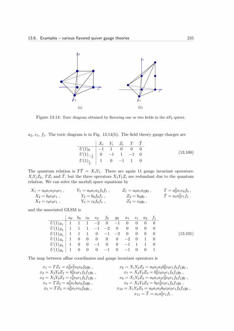
13.6. Examples – various flavored quiver gauge theories 235
(a) (b)
Figure 13.14: Toric diagram obtained by flavoring one or two fields in the dP0 quiver.
a2, e1, f1. The toric diagram is in Fig. 13.14(b). The field theory gauge charges are
Xi Yi Zi T T
U(1)0 −1 1 0 0 0U(1)− 1
20 −1 1 −1 0
U(1) 12
1 0 −1 1 0
(13.100)
The quantum relation is T T = X1Y1. There are again 11 gauge invariant operators:XiYjZk, TZi and T , but the three operators X1Y1Zi are redundant due to the quantumrelation. We can solve the moduli space equations by
X1 = a0a1a2e0e1 , Y1 = a0a1a2f0f1 , Z1 = a0a1a2g0 , T = a20a1e0f0 ,
X2 = b0e0e1 , Y2 = b0f0f1 , Z2 = b0g0 , T = a1a22e1f1 .
X3 = c0e0e1 , Y3 = c0f0f1 , Z3 = c0g0 ,
and the associated GLSM is
a0 b0 c0 e0 f0 g0 a1 e1 a2 f1U(1)B1 1 1 1 −2 0 −1 0 0 0 0U(1)B2 1 1 1 −1 −2 0 0 0 0 0U(1)B3 1 1 1 0 −1 −2 0 0 0 0U(1)B4 1 0 0 0 0 0 −2 0 1 0U(1)B5 1 0 0 −1 0 0 −1 1 1 0U(1)B6 1 0 0 0 −1 0 −1 0 0 1
(13.101)
The map between affine coordinates and gauge invariant operators is
x1 = TZ1 = a30a21a2e0f0g0 , x6 = X1Y2Z2 = a0a1a2b
20e0e1f0f1g0 ,
x2 = X2Y2Z2 = b30e0e1f0f1g0 , x7 = X2Y2Z3 = b20c0e0e1f0f1g0 ,x3 = X3Y3Z3 = c30e0e1f0f1g0 , x8 = X1Y3Z3 = a0a1a2c
20e0e1f0f1g0 ,
x4 = TZ2 = a20a1b0e0f0g0 , x9 = X2Y3Z3 = b0c20e0e1f0f1g0 ,
x5 = TZ3 = a20a1ce0f0g0 , x10 = X1Y2Z3 = a0a1a2b0c0e0e1f0f1g0 ,
x11 = T = a1a22e1f1 .

236 Chapter 13. Flavors in N = 2 toric Chern-Simons quivers
(a) The quiver. (b) Toric diagram.
Figure 13.15: The dP1 quiver with one flavor. Flavoring X112 has the effect of adding a new
point above two external points and one internal point in the toric diagram.
13.6.5 Flavoring the dP1 quiver
The dP1 quiver describes D-branes at the C(Y 2,1) CY3 singularity. The quiver has 4 nodesand 10 bifundamental fields, as section 3.5.4. The brane tiling and quiver are shown inFig. 3.4 and its perfect matchings are given in (3.52). Consider coupling a single flavorto the field X1
12, as in Figure 13.15(a). This time the field we flavor corresponds to twoexternal points b0 and c0, , as well as an internal point e0, in the toric diagram of dP1.The Chern-Simons levels are (12 ,−1
2 , 0, 0), which corresponds to adding three points b1,c1 and e1 in the toric diagram, as shown in Figure 13.15(b).
Xj12 Xi
23 Xi41 X31 X24 X34 T T
U(1) 12
1 0 −1 −1 0 0 1 0
U(1) 12−1 1 0 0 1 0 −1 0
U(1)0 0 −1 0 1 0 1 0 0U(1)0 0 1 1 0 −1 −1 0 0
(13.102)
The quantum relation is T T = X112. The F-term equations are solved by
X112 = b0b1c0c1e0e1 , X1
41 = c0c1h0 , X123 = c0c1f0 , X34 = b0b1g0 ,
X212 = a0b0b1e0e1 , X2
41 = a0h0 , X223 = a0f0 , T = b0c0e0 ,
X312 = d0e0e1 , X31 = d0g0h0 , X24 = d0f0g0 , T = b1c1e1 .
The GLSM is
a0 b0 c0 d0 e0 f0 g0 h0 b1 c1 e1U(1)B1 0 0 0 0 1 0 0 −1 0 0 0U(1)B2 0 0 0 0 −1 1 0 0 0 0 0U(1)B3 0 0 0 0 0 −1 1 0 0 0 0U(1)B4 1 0 1 1 −1 0 −1 −1 0 0 0U(1)B5 0 1 0 1 −1 −1 0 0 0 0 0U(1)B6 0 1 −1 0 0 0 0 0 −1 1 0U(1)B7 0 1 0 0 −1 0 0 0 −1 0 1
(13.103)
13.7. Conclusions 237
The three first lines correspond to the gauge charges under the first three gauge groups.Using the F-term relations together with T T = X1
12, one can show that there are only 10independent generators of the chiral ring,
x1 = X312X24X
141 , x4 = TX24X
241 , x7 = TX1
23X34X241 , x10 = T .
x2 = X312X24X
241 , x5 = X3
12X223X34X
241 , x8 = TX2
23X34X241 ,
x3 = TX24X141 , x6 = TX1
23X34X141 , x9 = X2
12X223X34X
241 .
and that they match the 10 affine coordinates of the toric geometry of Figure 13.15(b).
13.7 Conclusions
In this chapter, we studied the chiral ring of (conjectured) CFTs describing the IR fixedpoint of general 3d N = 2 supersymmetric quiver gauge theories with chiral flavors, withor without CS terms, focusing on the toric case. These CFTs are conjectured to beholographically dual to M-theory on AdS4 ×H7 backgrounds.
We have generalized the stringy derivation of the quiver theories [258] to cases wherethe M-theory circle degenerates at complex codimension-two loci in the toric CY4 cone,leading to flavor D6-branes wrapping toric divisors of the fibered CY3 in type IIA stringtheory. The holomorphic embedding of flavor branes determines the superpotential cou-plings between the (anti)fundamental flavor superfields and bifundamental matter in thedual theory, whereas the RR F2 fluxes contributed by D6-branes shift the CS levels.
Conversely, we have studied the addition of flavors coupled to bifundamental fields intoric 3d Abelian quiver theories. Flavoring is accompanied by shifts of some CS levelsin order to balance the parity anomaly. We proved that the geometric branch of themoduli space (the one where flavor fields do not acquire a VEV) of the chirally flavoredquiver theories is a toric conical CY4, and provided a recipe for deriving the toric diagram,exploiting an auxiliary quiver theory whose brane tiling has multi-bonds instead of flavors.The derivation of the moduli space relies on the existence of a non-trivial holomorphicOPE between BPS diagonal monopole operators, that we conjecture to appear at thequantum level since it is consistent with all global and gauge symmetries of the theory.Applying the reduction of [258] to the CY4 branch, we can provide a stringy derivationof the proposed flavored gauge theories, closing the circle.
Firstly, it would be interesting to explore the Higgs branches of the flavored theories.In the presence of intersecting D6-branes, it will be crucial to understand whether newsuperpotential interactions arising from flavor branes intersections can appear and bemarginal at the IR fixed point. The issue may be addressed using orbifold techniquesand following the result of partial resolutions, as suggested in [303].
Secondly, it would be nice to understand whether the auxiliary multi-bond branetilings are dual to the flavored quiver theories we studied. This issue requires the studyof the full flavored theory and A-theory moduli spaces. Partial resolutions, interpreted asHiggsings (removal of one edge in a multi-bond) in the A-theory, correspond to explicitbreaking of the flavor groups due to real mass terms in the flavored theory. Even thoughthis is reminiscent of mirror symmetry, the P- and A-theory are not geometric dual in thesense of [290]: they correspond to the same M-theory reduction. The stringy derivationnaturally leads to the flavored theory. Moreover, adding multi-bonds or flavorings are
238 Chapter 13. Flavors in N = 2 toric Chern-Simons quivers
local operations in the brane tiling/quiver, therefore any duality between the two theoriesmust be a local operation as well. Finally, notice that giving a VEV to a bifundamentalfield in the flavored theory not only Higgses the gauge groups but also gives mass toall flavors coupled to it. In the brane tiling of the A-theory, all the edges between twovertices are removed.
It would also be interesting to extend our analysis to the full class of ADE singularitiesin M-theory, which goes beyond the toric case: D-type singularities descend to orientifoldsin type IIA. One could also consider the addition of a Romans mass to the type IIA gravityduals with D6-branes, contributing a CS term to the diagonal gauge group [247, 309]:this would be particularly interesting for models with no CS terms, since it would providea manifestly conformal action in the sense of ABJM [202]. Finally, one could apply theprojection of [249] to identify N = 1 dual pairs with flavors.
Appendix A
Type IIB SUGRA action, chargesand equations of motion
We follow conventions according to which the action of Type IIB supergravity reads, inEinstein frame
SIIB =1
2κ2
∫
d10x√−g R − 1
2
∫ [
dΦ ∧ ∗dΦ+ e2ΦF1 ∧ ∗F1 +1
2F5 ∧ ∗F5
+ e−ΦH3 ∧ ∗H3 + eΦF3 ∧ ∗F3 − C4 ∧H3 ∧ F3
]
, (A.1)
where κ2 = π(2π)6α′4g2s is the Newton coupling constant and the gauge invariant fieldstrengths are defined as
F1 = dC0 , F3 = dC2 + C0H3 , F5 = dC4 + C2 ∧H3 , H3 = dB2 . (A.2)
In our conventions the Einstein frame is defined from the string frame by rescaling themetric by the fluctuating part of the dilaton field. Moreover, our RR fields are normalizedso as to appear in the action in a democratic way with respect to the NSNS fields, that isthe Newton coupling constant κ enters as an overall factor in front of the Einstein framesupergravity action. As a consequence, the dilaton field Φ appearing in the action (A.1) isits fluctuating part, only, as its VEV has been absorbed into κ. With these conventions,the world-volume action for a Dp-brane is
SDploc = −τp∫
Dpdp+1ξ e
p−34
Φ√
− det(g + e−Φ/2F) + τp
∫
C ∧ eF ∧ Ω9−p , (A.3)
where F = B2 + 2πα′ F2 (the hat on the NSNS 2-form means that the form is pulled-
back on the D-brane world-volume) and τp = 1/[(2π)pα′ p+12 gs]. Finally, C is a polyform
C =∑Cp, with Cp being all possible RR potentials (electric and magnetic), and Ω9−p
is a form localized on the Dp-brane worldvolume (the Poincare dual to the cycle) andclosed.
With these conventions, the D3-brane and D5-brane charges (so called Maxwell charges[184], see below) are, respectively
QD3 = −1
(4π2α′)2 gs
∫
F5 , QD5 = −1
4π2α′ gs
∫
F3 . (A.4)
239

240 Appendix A. Type IIB SUGRA action, charges and equations of motion
The equations of motion for the fields relevant to the solutions discussed in this thesisare
d eφ ∗ F3 = H3 ∧ F5 − 2κ2δSlocδC2
dF5 = −H3 ∧ F3 − 2κ2δSlocδC4
d e−φ ∗H3 = −F3 ∧ F5 − 2κ2δSlocδB2
,
(A.5)
where we have imposed self-duality of F5 on shell. By comparing the equations with theBianchi identities of the dual field strengths we get the relation
F7 = − eφ ∗ F3 . (A.6)
The BIs modified by D-brane sources are
dF3 = −2κ2δSlocδC6
dH3 = 0 . (A.7)
Remark that in our conventions, the complex 3-form G3 = dC2 + τH3 is simply
G3 = F3 + iH3 (A.8)
when the axio-dilation is constant.
A.1 Maxwell and Page charges for D3-branes
The charges defined in (A.4) are gauge invariant quantities, but they are not quantized ingeneral, because the Dirac quantization condition only applies to dC4 and dC2, which areclosed, while F5 and F3 are not closed in the presence of generic RR flux. Such chargeswere called Maxwell charges in [184].
Let us focus on the case of F5, with only F3 flux and no F1 flux, which is the case ofinterest in this thesis (we refer to [129] for a general discussion in the presence of D3-,D5- and D7-brane charges). The Page charge for D3-branes is defined as [184]
QPageD3 = − 1
(4π2α′)2 gs
∫
(F5 +B2 ∧ F3) . (A.9)
The form F5+B2∧F3 is closed in the absence of localized sources, since dF5 = −H3∧F3.Locally, F5 + B2 ∧ F3 can be written as d(C4 + B2 ∧ C2), so the Page charge will benon-zero only if there is some magnetic-monopole-like configuration. The Page charge isthen a topological quantity, and it is quantized.
However, the Page charge is not gauge invariant under large gauge transformations ofthe B-field, B2 → B2 + Λ2 for Λ2 some closed 2-form in a non-trivial cohomology class.

Appendix B
Algebraic geometry and toricgeometry
In this Appendix we will review the relevant mathematical concepts we need in algebraicgeometry, and particularly in toric geometry. The goal is to present toric geometry in itsnatural conceptual environement, which is algebraic geometry. All the relevant conceptsare introduced along the way. This introduction to toric geometry is based on lecturesgiven by the author at the Modave summer school in september 2008 [4].
Section B.1 is an introduction to the basic concepts of algebraic geometry. In sectionB.2 we will discuss the Calabi-Yau condition. In section B.3 we will delve into the coreof the subject, defining toric varieties as particular holomorphic quotients, and showinghow to introduce local coordinates in term of affine varieties (affine patches). Remarkthat we will mainly be interested in local properties, and so we will mostly concentrateon non-compact toric varieties. In particular we will consider Calabi-Yau toric varieties,which are always non-compact. In section B.4 we will introduce the notion of singularityin algebraic geometry, and we will show how we can deal with singular points in thetoric case. In section B.5 we introduce a second way to define toric varieties, the Kahlerquotient, also known as gauged linear sigma-model.
The presentation aims to be as self-contained as possible, but general knowledge ofcomplex geometry is assumed at some point, especially in section B.2. Good introductionsto complex geometry and Calabi-Yau manifolds can be found for instance in [310, 311,312]. A very interesting mathematical reference is [313]. The standard reference on toricgeometry is [314]. Posterior developments as explained in [315] are also important, asthey actually simplify matters. See [316] for a nice account from a physicist perspective.
B.1 Algebraic geometry: the gist of it
We know that in geometry we always deal with some bunch of “points” that has moreor less structure to it. A set of points together with a topology is called a topologicalspace. Recall that a topology is what you define to be the open sets in your space, henceit provides a notion of locality. A topological space that locally looks like the euclidianspace Rn is called a manifold. If moreover the transition functions are differentiable (C∞
for instance), it is called a differentiable manifold.
241
242 Appendix B. Algebraic geometry and toric geometry
Smooth algebraic varieties can be seen as particular kind of manifolds which aresimpler in some sense. Roughly speaking, they can be thought of as manifolds withrational transition functions1. On the other hand, generic algebraic varieties are notmanifolds, since they allow for various singularities; in that sense they are more general.
Remark that it is possible to define algebraic varieties intrinsically, in a way similarto what one does in differential geometry, but for doing so we would need to introducethe language of sheaves, and that would carry us too far afield. We will follow the moredown to earth route, which defines algebraic varieties extrinsically as the algebraic set ofzeros of some polynomials. Given a function f : Rn → R, we can define a subset of Rn,
Rn ⊃ Σ = f−1(0) = x ∈ R
n | f(x) = 0,
which locally inherits its manifold structure from Rn. However, this Σ is badly singular
in general. If we restrict f to be a polynomial, things become much more tractable. It isone of the great advantages of the algebraic side of algebraic-geometry that singularitiesbecome easier to deal with.
Therefore we are now considering algebraic equations only. Hence it is very convenientto work with polynomials valued in C, because C is algebraically complete. From nowon, unless otherwise stated, all variables are C-valued, and by dimension we always meancomplex dimension (half the real dimension).
Some algebraic definitions and propositions are reviewed in Insert 5, without demon-strations. For more details, see any algebraic geometry textbook, such as [317].
In this section we will first define affine varieties, which are the basic objects ofalgebraic geometry. Next we define the projective space CPn, which provides us witha particular example of the holomorphic quotient construction that we will encounterin detail when we define toric varieties in section B.3. For completeness we also defineprojective varieties, which are subvarieties of CPn.
B.1.1 Affine varieties
Varieties defined as algebraic subset of Cn lead to the concept of affine varieties. ConsiderCn = (x1, · · · , xn). Associated to it, we have the ring of polynomials in n variables,
which is denoted byRn ≡ C[x1, · · · , xn] . (B.2)
It is obviously a ring (it is an additive group together with an associative product, dis-tributive with respect to the addition); moreover it is a commutative ring. An algebraicsubset Z(T ) of Cn is defined as the zero locus of a set of polynomials T ⊂ Rn:
Z(T ) = (x1, · · · , xn) ∈ Cn | pi(x1, · · · , xn) = 0, ∀pi ∈ T . (B.3)
On the other hand, for any subset Y ⊂ Cn, we denote the set of all polynomials that
vanish on Y by J (Y ). A natural question to ask is what is the relation between J (Z(T ))and T . This is the content of the famous Hilbert’s Nullstellensatz.
The whole idea of algebraic geometry is that you can define a space by the algebra offunctions defined on it2. Let us look at the polynomials which give rise to well defined
1For toric varieties we will see that it is precisely that.2Note that the ring of polynomials is naturally an algebra too.

B.1. Algebraic geometry: the gist of it 243
Insert 5. A few notions of algebra
Ring. A ring is a set R equipped with two binary operations, + and ·, such that(i) (R,+) is a commutative group,(ii) · is associative and there exist a neutral element (called unity). If moreover · is commutativewe talk of a commutative ring (it is the case in these lectures).(iii) · is distributive over + .Examples: The sel of all integers Z is a ring. Another example is the ring of polynomials in nvariables, denoted C[x1, · · · , xn].
Ideal. An ideal I of a ring R is a subset I ⊂ R such that(i) i, j ∈ I ⇒ i− j ∈ I,(ii) i ∈ I, r ∈ R ⇒ ir ∈ I.
Proposition: I an ideal of R implies that the quotient R/I is a ring too.
Notation: Given a set of elements r1, · · · , rk ⊂ R, we denote (r1, · · · , rk) the idealgenerated by this set, which is the smallest ideal of R containing r1, · · · , rk.
Prime ideal. An ideal P ⊂ R is a prime ideal if for any ideals I, J ⊂ R,
I · J = ij ∈ R | i ∈ I, j ∈ J ⊂ P ⇒ I ⊂ P or J ⊂ P.
Example: In the ring C[x, y], the ideal (xy) is not prime. It has a primary decomposition into(x) and (y).
Radical of an ideal. Let I be an ideal of R. The radical of I, denoted rad(I), is theintersection of all the prime ideals containing I. (rad(I) is itself an ideal.)Example: In C[x, y], rad((xnym)) = (xy).
An ideal I ⊂ R is said to be radical if rad(I) = I.
Height of a prime ideal. The height h(P ) of a prime ideal P ⊂ R is the largest integer hsuch that there exist a chain of strict inclusions of prime ideals Pi
P0 ⊂ P1 ⊂ · · · ⊂ Ph = P . (B.1)
It gives a notion of the dimension of an ideal. Moreover it can be shown that the dimensionof the affine variety corresponding to the quotient ring C[x1, · · · , xn]/P is n− h(P ).
Zero divisor and integral domain. An element r ∈ R, r 6= 0, is called a zero divisor ifthere exists s ∈ R, s 6= 0, such that rs = 0. A commutative ring without zero divisor is calledan integral domain.
Proposition: Given R an integral domain, and I ⊂ R an ideal, then R/I is an integraldomain if and only if I is prime.
244 Appendix B. Algebraic geometry and toric geometry
functions on the algebraic set (B.3). Two polynomials p1 and p2 will take the same valueon Z(T ) if p1 − p2 = t, with some t ∈ T , since t vanishes on Z(T ) by definition. Wethen only need to consider the equivalence classes of polynomials in Rn that are linearlyequivalent up to elements of T . This is denoted by
A(Z(T )) = C[x1, · · · , xn]/T . (B.4)
We want this quotient to define a proper ring of functions on Z(T ). This happens if Tis an ideal of the ring C[x1, · · · , xn]. An ideal of a ring R is a subset I ⊂ R such that Iis a subgroup for the addition and is invariant under multiplication by any element in R.Given any set of polynomials, it is not difficult to extend it into a full-fledged ideal, asone can see in the examples below. One usually denote the ideal generated this way by(p1, · · · , pk).
Examples:
• Take the ring C[x] of polynomials in x. The set x is not an ideal (for instance itis not even a subgroup), but we can generate one simply by multiplying with everyelement of C[x]. The ideal, denoted (x), is simply the set of all polynomials withoutconstant term. The quotient by the ideal simply gives the constants:
C[x]/(x) = C. (B.5)
• Consider the ideal (x2) instead. The quotient C[x]/(x2) is a ring generated by thetwo elements 1, x such that x.x = 0. Such a x is called a zero divisor.
• On the ring C[x, y], consider the ideal (xy). The quotient ring C[x, y]/(xy) has twozero divisors (x and y).
This last example corresponds to the surface xy = 0 in C2. It consists of two branches
which meet at the origin. In general, any algebraic set will consist of several “branches”,
Z(T ) = Σ1 ∪ · · · ∪ Σm, (B.6)
and correspondingly the quotient ring (B.4) will have zero divisors. To avoid zero divisors,one must ask that the ideal be prime (see the Appendix 5 for the definition). In ourexample, (xy) is not prime, but it has a decomposition in two prime factors (x) and (y).These two ideals correspond to the two “branches” x = 0 and y = 0.
Each component in the decomposition (B.6) is called irreducible if it cannot be de-composed further.
Definition: An affine variety is an irreducible algebraic subset of Cn.
It is called “affine” simply because it is defined in Cn, which is an affine space (i.e.
a vector space where you can shift the origin anywhere). The very important thing toremember is that there is a one-to-one correspondence between affine varieties and primeideals:
Σ = Z(P )1−1←→ A(Σ) = C[x1, · · · , xn]/P. (B.7)
B.1. Algebraic geometry: the gist of it 245
Insert 6. Hilbert’s Nullstellensatz
Consider an ideal I of C[x1, · · · , xn]. Given the algebraic subset Z(I) ⊂ Cn, as defined in
section B.1.1, is the knowledge of Z(I) enough to reconstruct the ideal I? The answer is thatyou can only find rad(I). This is the content of the famous Hilbert’s Nullstellensatz. Moreprecisely: Theorem. For any ideal I of C[x1, · · · , xn],
J (Z(I)) = rad(I),
where J (Z(I)) is the set of all polynomials vanishing on Z(I).
We then have a one-to-one correspondence between algebraic sets and radical ideals. Remarkthat in dimension one, it implies that a polynomial with isolated zeros is fully determinedby its roots; the Nullstellensatz is a generalisation of the fundamental theorem of algebra tohigher dimensions.
This is a consequence of the Hilbert’s Nullstellensatz (see Insert 6), which implies thatif T = P is a prime ideal then the set of polynomials vanishing on Z(P ) is P itself,J (Z(P )) = P .
Definition: The ring A(Σ) defined as in (B.4),
A(Σ) = C[x1, · · · , xn]/P, (B.8)
is called the coordinate ring, or structure ring, of the affine variety Σ. This constructionis familiar from supersymmetric theories: there the xi are the gauge invariants operators,and P is generated by the F-terms. The structure ring in that case is called the chiralring.
Example: the conifold. The ubiquitous conifold, C0, which has been such a cen-tral tool in recent developments in string theory, is an affine variety defined by a singleequation in C
4,x1x2 − x3x4 = 0. (B.9)
Mathematicians call it a “threefold ordinary double point”, or node. Its coordinate ringis
A(C0) = C[x1, x2, x3, x4]/(x1x2 − x3x4). (B.10)
B.1.2 Projective varieties
Affine varieties, being defined by polynomial equations in Cn, are not compact. The
projective space CPn is the simplest example of a compact algebraic variety (actually itis toric too). The standard way to define it is as the set of complex lines in C
n+1,
CPn =(Cn+1\0)
C∗. (B.11)
The action of C∗ = C\0 is to multiply all coordinates in Cn+1 by λ ∈ C
∗, which definesthe equivalence relation
[x0, · · · , xn] ∼ [λx0, · · · , λxn]. (B.12)

246 Appendix B. Algebraic geometry and toric geometry
The origin 0 was removed before taking the quotient so that C∗ may act freely. The
resulting space is fully regular. The xi are called homogeneous coordinates, and a pointin CPn is represented by the equivalence class [x0, · · · , xn]. We can cover CPn with n+1
affine patches, one for each xi 6= 0. The local coordinates on the i-patch are z(i)k = xk/xi,
and the transition functions are the rational functions
z(i)k (z(j)) =
z(j)k
z(j)i
. (B.13)
The Riemann sphere CP1 is the best known example. It has two patches, and thetransition function on the equator is zN = 1/zS .We can define subvarieties of CPn by taking the vanishing locus of a set of polynomialspi ∈ Rn+1. For the equations pi = 0 to make sense, they should be constant on anyequivalence class [x0, · · · , xi], which means the p’s are homogeneous (i.e. they are sumsof monomials of fixed degree):
pi(x0, · · · , xn) ∼ λdpi(x0, · · · , xn). (B.14)
Definition: Given a homogeneous prime ideal Ph in Rn+1, the associated projectivevariety is defined as
Σ(Ph) = [x0, · · · , xn] | pi = 0 ∀pi ∈ Ph ⊂ Rn+1. (B.15)
It is easy to check that if the pi’s are homogenous of degree d, so is the ideal (pi).The homogeneous coordinate ring is denoted by
S(Σ) = Rn+1/Ph . (B.16)
Projective plane curves. In CP2, consider a hypersurface defined by a singlepolynomial p of degree d. If moreover
∂p(x)
∂xi= 0 ∀i, ∀x s.th. p(x) = 0 , (B.17)
the curve is regular; it is a Riemann surface. Such Riemann surfaces are classified bytheir genus. There exists a theorem stating that
g =(d− 1)(d− 2)
2. (B.18)
In particular, for d = 3, we have a torus, or elliptic curve (g = 1). The general equationreads ∑
i+j+k=3
cijk xi0xj1xk2 = 0. (B.19)
We have 10 parameters here. However 9 of them can be removed by a Gl(3,C) trans-formation on the homogeneous coordinates. This leaves us with one parameter, which isbasically the complex structure modulus of the torus. We will come back to the impor-tant issue of complex structure moduli later on in these lectures.
Remark that there are many more algebraic varieties than just affine and projectiveones. In general, one can patch together affine varieties to obtain any algebraic variety,similarly to the idea of patching together open sets to form manifolds in differentialgeometry. We will see this explicitly in the simpler context of toric varieties.
B.2. The Calabi-Yau condition 247
B.1.3 Spectrum and scheme, in two words
Let us introduce the notion of spectrum of a ring. This is done only to set a usefulnotation that you might often encounter in the literature. The concepts of spectrum andscheme stem from taking seriously the idea that it is really the algebra of functions on itwhich defines a space. One starts with a purely algebraic object : given any ring A, onedefines its spectrum
Spec(A) ≡ P ⊂ A, (B.20)
to be the set of all prime ideals of A (except A itself). This set can be given a naturaltopology, and it is then shown that, in the particular case of the coordinate ring of anaffine variety,
Spec(A(Σ)) ∼= Σ, (B.21)
up to important subtleties that we shall willfully skip (in particular we are really talkingabout the maximal ideals here). The scheme structure is then obtained by introducinglocal coordinates by means of a so-called structure sheaf (for interesting introductions tosheaf concepts in physics, see for instance [48, 49]).
B.2 The Calabi-Yau condition
In this section we consider algebraic manifolds, i.e. non-singular algebraic varieties. It isfair to warn the reader that we will be applying results of this section in singular casesin the next section, although we will not discuss how this can be rigorously done.
An algebraic manifold is obviously a complex manifold: all the quantities we are deal-ing with are holomorphic by construction, and the variety inherits its complex structurefrom the embedding space C
n or CPn. In this section, since we deal with manifolds, wecan take a more direct, “intrinsic”, differential-geometric standpoint. This will simplifymatter, since differential geometry is bound to be more familiar to the reader.
B.2.1 Holomorphic vector bundles and line bundles
Consider a complex manifold X of dimension m. On every open set we have local coor-dinate functions z1, · · · , zm, and we can define the exterior algebra of these coordinatefunctions, generated by one-forms
dz1, · · · , dzm. (B.22)
At any point p in the open set, dzi(p) form a basis for the holomorphic cotangent spaceT ∗pX at p. The multiplication operation on forms is the exterior product. All in all we
have 2m linearly independent elements
1, dzi, dzi1 ∧ dzi2 , · · · , dzi1 ∧ · · · ∧ dzim , (B.23)
which form a graded algebra. At each degree, p-forms at any particular point span avector space of dimension n!
p!(n−p!) .
Using holomorphic Gl(m,C)-valued transition functions, we can patch all cotangentspaces together into the holomorphic cotangent bundle T ∗X:
Cm −→ T ∗X
π−→ X , (B.24)

248 Appendix B. Algebraic geometry and toric geometry
which is itself a manifold of dimension 2m. This is a particular case of an holomorphicvector bundle E,
Ck −→ E
π−→ X , (B.25)
with Ck the fiber, and π the natural projection, which is an holomorphic map. k is called
the rank of the bundle.Definition: An holomorphic line bundle (or line bundle for short) is an holomorphic
vector bundle of rank one.A very important line bundle is the canonical bundle KX . It is defined as the mth
exterior product of T ∗X,
C −→ KX ≡ Λ(m,0)T ∗Xπ−→ X . (B.26)
Sections of the canonical bundle are holomorphic m-forms, that we can write (on eachcoordinate patch)
Ω = f(z)dz1 ∧ · · · ∧ dzm, (B.27)
for f(z) some holomorphic function.
B.2.2 Calabi-Yau manifolds. Kahler and complex moduli
The Calabi-Yau condition is that the canonical bundle be trivial, i.e.
Λ(m,0)T ∗X ∼= C × X . (B.28)
This implies the existence of a never vanishing global section. Standard arguments thenimply that the function f(z) in (B.27) must be a constant. This unique (up to rescalingby a constant) Ω is usually called the holomorphic m-form of the Calabi-Yau manifoldX.
Kahler structure. A complex manifold can be endowed with a Kahler structure.There is no room here to explain in detail what this is, see [310, 311]. In two words though,a Kahler structure is a symplectic structure compatible with the complex structure: youneed a closed and non-degenerate (1, 1)-form ω. The nice thing is that complex structureplus Kahler structure implies there is a compatible Riemannian structure, i.e. a hermitianmetric. This metric is defined by
g(∂z, ∂z) = ω(∂z, i ∂z) (B.29)
for any two vectors ∂z, ∂z in the tangent space (holomorphic and anti-holomorphic). TheKahler form ω is a representative of a Dolbeault cohomology class
[ω] ∈ H1,1(X). (B.30)
[ω] is called the Kahler class of ω.Now, we can state Yau’s theorem (Yau proved a conjecture made earlier by Calabi):
CY Theorem : Given X a compact complex manifold with trivial canonical bundle, andgiven a Kahler form ω on X, there exist a unique Ricci flat metric in the Kahler class ofω. That is, a unique Ricci-flat metric given by (B.29) for some ω ∈ [ω].
On the other hand, it is “easy” to show that Ricci-flatness implies the triviality of theline bundle. For a non-compact manifold, the theorem does not hold (strictly speaking).

B.2. The Calabi-Yau condition 249
One can still find a Ricci-flat metric in general, but one must specify some boundaryconditions at infinity.
Kahler moduli space. Given a Calabi-Yau manifold X, we see there are continuousfamilies of Ricci-flat metrics, one for each cohomology class
[ω] =h1,1∑
i=1
λi [ω]i . (B.31)
These parameters λ are coordinates in a vector space H1,1(X) (here the [ω]i are basisvectors). It is called the Kahler moduli space of X. Its dimension is denoted by h1,1.
Complex moduli space. Given an algebraic variety, if one modifies the equationcontinuously, varying some parameters, the variety will be “deformed” accordingly. Thisis called a variation of the complex structure.
Consider the example of the torus of section B.1.2; we saw there are 10 parametersone can vary, but 9 of them do not change the complex structure, because they are justa linear reshuffling of the embedding space coordinates, so the complex moduli space ofthe torus is one dimensional.
Consider also the conifold, defined by x1x2 − x3x4. If I write, for instance,
x1x2 − bx3x4 + cx4 = 0, (B.32)
the constants b and c can obviously be absorbed in a redefinition of x3, with x′3 = bx3−c.
For an affine variety in Cn, we can transform the variables by
Gl(n,C)⋉ Tn, (B.33)
with Tn the group of translations. In the case of C0 in C4, we have 15 possible parameters
for a generic polynomial of degree 2. However most of them can be removed by aGl(4,C)⋉T4 transformation. One can check that the only parameter which cannot be removed bysuch a transformation is the constant term,
x1x2 − x3x4 − a = 0. (B.34)
Such a space is called the deformed conifold, and it is regular.The space of all complex deformations of an algebraic variety X is called the complex
moduli space of X. It is a rather complicated space. Its linearisation (the tangentspace) is given by the cohomology group Hm−1,1(X) (m the dimension of X) in the caseof Calabi-Yau manifolds. In general, the question is much more complicated. In theparticular case of the theory of complex deformations of toric Calabi-Yau singularities,there is some important results to be learned, as we will see.
B.2.3 Divisors and line bundles
Definition: A (Weyl) divisor D of a complex variety X is a linear combination (aformal sum with integer coefficients) of codimension one irreducible subvarieties,
D =∑
i
niVi, ni ∈ Z, Vi ⊂ X. (B.35)

250 Appendix B. Algebraic geometry and toric geometry
If all ni ≥ 0, the divisor D is said to be effective.To any line bundle L with a regular section s (which means that on any open set Uα,
sα is a polynomial in the local coordinates) we have an associated hypersurface Y in Xdefined by
Y = s(p) = 0, p ∈ X. (B.36)
We can decompose Y into irreducible parts. On any affine patch, the polynomial sαcan be factorized in C[x1, · · · , xn]. In fact, (sα) is decomposed into prime ideals, andone keeps track of the multiplicity3 ni of each distinct ideal Pi. The prime ideal Picorresponds to the subvariety Vi in (B.35). More precisely, one should of course patch allthe V α
i together to construct Vi ⊂ X.Going the other way around, an effective divisor D =
∑
i niVi defines a line bundle,denoted OX(D). By definition its sections will vanish on each Vi with a zero of order ni.
On can generalize this construction to any divisor, where now ni < 0 corresponds toa pole of order ni for the corresponding sections of OX(D).
Example. On X = CPn, we can set zi = 0 (zi an homogeneous coordinate). Itcorresponds to the hyperplane H (any Hi = zi = 0 is linearly equivalent to the others).A general divisor is then D = nH, n ∈ Z. Its associated line bundle is usually denotedO(n). Note that O(−1), corresponding to D = −H, is really the dual of the hyperplaneline bundle (i.e. its sections are in Hom(O(1),C)). It is called the tautological line bundleof CPn.
B.3 Toric geometry 1: The algebraic story
We are now ready to discuss toric geometry. In this section we define a toric variety as aparticular holomorphic quotient (or GIT quotient) of Cn.
Definition: A toric variety X (of dimension m) is an algebraic variety containingthe algebraic torus T = (C∗)m as a dense open subset, together with a natural actionT×X → X.
We can write X as
X∆ =Cn\Z∆
G. (B.37)
Here, the groupG ∼= (C∗)n−m × Γ, (B.38)
is an algebraic torus times an abelian discrete group Γ. This construction generalizesthe one for projective spaces. For it to make sense, we have to specify a set of pointsZ∆ ⊂ C
n, and of course we must know how G acts on Cn.
B.3.1 Cones and fan. Homogeneous coordinates
All this data defining a toric variety can be encoded in a simple auxiliary object called afan. Hence the fan can be taken to define the toric variety. An equivalent definition willbe in term of the gauged linear sigma-model of section B.5: the same data is present inboth definitions, in particular the charge matrix to be defined momentarily. Moreover,
3There is a multiplicity because the ideal (sα) is not radical in general.

B.3. Toric geometry 1: The algebraic story 251
this data is combinatoric, which means that is is given by discrete quantities. What makestoric geometry attractive is that complicated geometric problems can often be reducedto simpler combinatoric problems.
Let N ∼= Zm be a lattice, and NR = N ⊗R the vector space obtained by allowing real
coefficients.
Definition: A strongly convex rational polyhedral cone σ ⊂ NR, or cone for short,is a set
σ = ∑
i
aivi | ai ≥ 0, (B.39)
generated by a finite set of vectors vini=1 in N , and such that σ ∩ (−σ) = 0 (“strongconvexity”).
Definition: A fan is a collection ∆ of cones in NR such that(i) each face of a cone is also a cone,(ii) the intersection of two cones is a face of each.
Let us call ∆(1) the set of one-dimensional cones in NR. The corresponding vectorsin N are denoted (v1, · · · , vn). To each vi, one associates a homogeneous coordinate zi.These are the coordinates on C
n in the holomorphic quotient construction (B.37).Remark that we always have n ≥ m. The (m× n) matrix
(vki ) = (vk1 , · · · , vkn) (B.40)
(with k = 1, · · · ,m) induces a map
φ : Cn → Cm : (z1, · · · , zn) 7→ (
∏ni=1z
v1ii , · · · ,
∏ni=1z
vmii ). (B.41)
We define G = (C∗)n−m ⊂ G to be the kernel of φ:
G = Ker(φ). (B.42)
It is easily seen that G acts on Cn as
G ⊃ (C∗)a : (z1, · · · , zn) 7→ (λQa1z1, · · · , λQ
anzn) (B.43)
for each a, where the charge vectors Qa are in the kernel of the linear map (B.40), thatis: ∑
i
(vki )Qai = 0. (B.44)
Hence, practically speaking, given a fan with n vectors in N we must find the n − mlinear relations among them. The coefficients are precisely the Qai above.
The discrete group Γ ⊂ G is defined as
Γ = N/N ′ , (B.45)
where N ′ ⊂ N is the sublattice generated over Z by the vectors vi. The quotient by thisΓ gives rise to so-called orbifold singularities.

252 Appendix B. Algebraic geometry and toric geometry
Figure B.1: The toric fan of CP2. Notice that it contains 7 cones: three top-dimensional ones(of dimension 2), three 1-dimensional ones (generated by the vectors), and a single 0-dimensionalone (the point in the center).
Last but not least piece of data in the construction, the zero set Z∆ is found as follows:For any subset of ∆(1) (corresponding to vectors vi1 , · · · , vil) which do not generate acone in ∆, associate an algebraic set Vi1,··· ,il defined by zi1 = · · · = zil = 0. Then Z∆ isthe union of all these subsets of Cn.
We’d better move on to examples.
• Consider the fan in figure B.1, generated by 3 vectors in N ∼= Z2:
v1 = (1, 0), v2 = (0, 1), v3 = (−1,−1). (B.46)
The one relation v1 + v2 + v3 = 0 gives a single charge vector (see (B.44))
Q = (1, 1, 1), (B.47)
so we have the following group action of G = C∗ on the homogeneous coordinates:
G : (z1, z2, z3) 7→ (λz1, λz2, λz3). (B.48)
Moreover, one sees that Z∆ = (0, 0, 0). The construction obviously gives us CP2
as defined earlier.
• The (singular) conifold C0 is a 3-dimensional affine variety. It is not difficult torealize that a toric affine variety can only correspond to a single top-dimensionalcone in the fan (see below). The fan for the conifold contains 10 cones (includingthe 0-dimensional one). It is generated by four lattice vectors in N ∼= Z
3:
v1 = (0, 0, 1), v2 = (1, 0, 1), v3 = (1, 1, 1), v4 = (0, 1, 1). (B.49)
There is a single relation with charge vector (1,−1, 1,−1), so G is one dimensionaland acts as
G : (z1, z2, z3, z4) 7→ (λz1, λ−1z2, λz3, λ
−1z4). (B.50)
The zero set isZ∆ = z1 = z3 = 0 ∪ z2 = z4 = 0. (B.51)

B.3. Toric geometry 1: The algebraic story 253
B.3.2 Coordinate rings and dual cones
The homogeneous coordinates are very useful for many purposes. However, it is natural toask how we can describe a toric variety in local coordinates: as for manifolds, we wouldlike to be able to cover our varieties with open sets equipped with local coordinates.The relevant notion of open sets is different here from the usual topology of differentialgeometry4, but this will not concern us here. We should say, however, that because wedeal with singular spaces, the most “local” one can get is to affine varieties themselves.This is why it was so crucial to spend some time introducing them. Moreover, becausethe only non-singular affine variety is C
m itself, for non-singular varieties the relevantopen sets are simply C
m and we recover the usual notions for complex manifolds, whichwe used in section B.2.
How do we find such local coordinates? The fan again provides the answer. Toeach top-dimensional cone we associate an affine variety (affine patch). The transitionfunctions between these patches are also naturally encoded in the fan.
Given a single m-dimensional cone σ spanned by n vectors, we want to find thecoordinate ring associated to it. Since a toric variety is defined as a quotient by G, localcoordinates should be G-invariant polynomials5:
x = zn11 · · · znnn , G : x 7→ λ
∑
iQai nix = x, (B.52)
which means that the positive integers ni are such that∑
iQai ni = 0. Because of (B.44),
this means that we can take
ni = 〈w, vi〉 (B.53)
for any w ∈ Hom(N,Z) : The local coordinates are in one-to-one correspondence withelements in the dual lattice M ∼= Z
m,
M = Hom(N,Z). (B.54)
In fact, the condition ni ≥ 0 defines the dual real cone σ∨ ∈MR,
σ∨ = aw ∈MR | a ∈ R≥0, 〈w, vi〉 ≥ 0 ∀vi ∈ σ. (B.55)
Then, the coordinate ring we are looking for is simply
Aσ = C[σ∨ ∩M ]. (B.56)
Indeed σ∨ ∩M is a semi-group defining the monomials in the ring, and the addition inσ∨ ∩M becomes the multiplication in the ring. One can easily write this as the quotientof a polynomial ring by some ideals:
• First, find a minimal set of lattice vectors (w1, · · · , wr) generating σ∨ ∩ M ; ingeneral this is the most tricky part of the construction. We associate to this set thepolynomial ring Rr = C[x1, · · · , xr].
4The natural topology in algebraic geometry is called the Zariski topology. See any textbook such as[317].
5The reader should generalize the following considerations to the case when G has a non-trivial discretesubgroup Γ. See the examples below.

254 Appendix B. Algebraic geometry and toric geometry
• Find all the relations between the w′is, and associate to each relation an element of
Rr:∑
i∈I
miwi =∑
j∈J
mjwj , mi,mj ∈ N ⇒ p(x) =∏
i∈I
xmii −∏
i∈J
xmii (B.57)
where I ∪J = 1, · · · , r and I ∩J = 0. This generates a prime ideal Pσ = (p), andwe then have
Aσ = C[σ∨ ∩M ] =C[x1, · · · , xr]
(p). (B.58)
It is not obvious but nonetheless true that this ideal is prime, and moreover it is suchthat the associated affine variety
Uσ = Spec(C[x1, · · · , xr]
Pσ) (B.59)
has dimension m6. Here we used the notation of (B.21).The affine varieties Uσi , σi ∈ ∆, can be patched together to form a more general toric
variety X∆. Suppose the cone τ is a face of both σi and σj . Then, we have that
σ∨i, j ⊂ τ∨ ⇒ C[σ∨i, j ∩M ] ⊂ C[τ∨ ∩M ] ⇒ Uτ ⊂ Uσi ∩ Uσj . (B.60)
In words, the affine set associated to the face is in the intersection of the affine sets ofthe two cones. Hence the relations between local coordinates in x(i) for Uσi and x
(j) forUσj can be read off from the relations between the generators of σ∨i ∩M and σ∨j ∩M :
ri∑
l=1
qlw(i)l =
rj∑
l′=1
ql′w(j)l′ , ql,l′ ∈ Z ⇒
ri∏
l
(x(i)l )ql =
rj∏
l′
(x(j)l′ )ql′ (B.61)
We see that the transition functions are always rational functions.
Examples:
• Consider again the fan for CP2. There are three 2-dimensional cones, σ1, σ2, σ3,and for each of them
Uσi = Spec(C[σ∨i ∩M ]) ∼= C2. (B.62)
Applying (B.61), we see that the transition functions between Uσ1 = (x1, x2) andUσ2 = (y1, y2), for instance, are
x1 =y1y2, x2 =
1
y2. (B.63)
• Consider the simple fan in N ∼= Z2 shown in the Fig.B.2(a). It has a single topdimensional cone, spanned by
v1 = (1, 1), et v2 = (1,−1). (B.64)
6This means that the height of the ideal Pσ is always r −m.
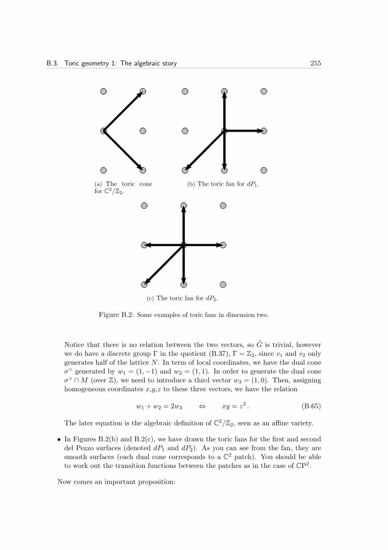
B.3. Toric geometry 1: The algebraic story 255
(a) The toric conefor C2/Z2.
(b) The toric fan for dP1.
(c) The toric fan for dP2.
Figure B.2: Some examples of toric fans in dimension two.
Notice that there is no relation between the two vectors, so G is trivial, howeverwe do have a discrete group Γ in the quotient (B.37), Γ = Z2, since v1 and v2 onlygenerates half of the lattice N . In term of local coordinates, we have the dual coneσ∨ generated by w1 = (1,−1) and w2 = (1, 1). In order to generate the dual coneσ∨ ∩M (over Z), we need to introduce a third vector w3 = (1, 0). Then, assigninghomogeneous coordinates x,y,z to these three vectors, we have the relation
w1 + w2 = 2w3 ⇔ xy = z2 . (B.65)
The later equation is the algebraic definition of C2/Z2, seen as an affine variety.
• In Figures B.2(b) and B.2(c), we have drawn the toric fans for the first and seconddel Pezzo surfaces (denoted dP1 and dP2). As you can see from the fan, they aresmooth surfaces (each dual cone corresponds to a C
2 patch). You should be ableto work out the transition functions between the patches as in the case of CP2.
Now comes an important proposition:
256 Appendix B. Algebraic geometry and toric geometry
Proposition: A toric variety X∆ is compact if and only if its fan ∆ spans the wholeNR.
See Chapter 2 of [314] for a proof. One sees in the above examples that CP2 anddP1,2 are compact spaces, while C
2/Z2 or the conifold are of course not.
B.3.3 Calabi-Yau toric varieties
In this subsection, we show how the Calabi-Yau condition is translated into a simplecondition on the combinatoric data for X∆.
We saw in section B.2 that the Calabi-Yau condition for X is the triviality of thecanonical bundle KX . Here we show how one can express KX in term of a simple set ofdivisors called toric divisors.
Definition: A toric divisor is a divisor invariant under the action of G.
Using the homogeneous coordinates (zi), we can easily define subvarieties that areG-invariant. Indeed, the simple algebraic sets
(z1, · · · , zn) | zi = 0 ∀i ∈ I ⊂ 1, · · · , n. (B.66)
are obviously G-invariant. In particular, the subvarieties
Di ≡ zi = 0 ∩X∆ (B.67)
are toric divisors 7. They actually generate the full group of divisors of X∆.Consider X∆ smooth with canonical bundle KX . One can show that
KX = OX(−n∑
i
Di) . (B.68)
The argument goes as follows. Because X∆ is regular, each coordinate ring Aσ is freelygenerated:
Uσ ∼= Ck × (C∗)m−k, ⇔ Aσ = C[x1, · · · , xk, xk+1, x
−1k+1, · · · , xm, x−1
m ] . (B.69)
Consider for simplicity the case k = m, which means σ is of dimension m (the general-ization is straightforward). A section of the canonical bundle is
Ω =1
x1 · · ·xmdx1 ∧ · · · ∧ dxm. (B.70)
This section corresponds to a divisor. Equivalently, the dual section in K−1X corresponds
to an effective divisor, described locally by
x1 · · ·xm = 0 ∩ Uσ. (B.71)
It is called the anti-canonical divisor.
7This is because the ideal (zi) has height one, which implies Di is codimension one in X∆ too.

B.3. Toric geometry 1: The algebraic story 257
On the other hand, a section of the line bundle O(∑iDi) corresponds to the divisor
z1z2 · · · zn = 0 ∩X ⊂ X. (B.72)
We know that
x1 · · ·xm = z〈w,v1〉1 · · · z〈w,vn〉n with w =
m∑
j
wj . (B.73)
Suppose the first m vectors amongst the vi’s span the cone σ. Since Uσ ∼= Cm, we have
〈w, vi〉 = 1 for i = 1, · · · ,m. Hence the anti-canonical divisor corresponds to∑
iDi onUσ. This implies that K−1
X = O(∑ni Di), which is what we wanted to show.
The important relation (B.68) allows us to state the Calabi-Yau condition (trivialityof the canonical bundle) in a very simple way. Note that any G-invariant function, asdefined in (B.52), is of course a section of the trivial bundle. We then see that OX(
∑
iDi)is trivial if and only if
G : z1 · · · zn 7→ λ∑
iQai (z1 · · · zn) = z1 · · · zn ⇔
∑
i
Qai = 0, (B.74)
or equivalently if there exist a dual vector w ∈ M such that 〈w, vi〉 = 1 for all vi in thefan. We then have shown the following:
Proposition: The toric variety X∆ is Calabi-Yau if and only if all the vectors vi in∆ end on the same hyperplane in N , which happens if and only if
∑
iQai = 0 ∀a.
Remark that we chose the vi for the conifold in (B.49) especially to make the CYproperty explicit.
It also follows from the proposition at the end of the last subsection that a toric CYcannot be compact.
B.3.4 Toric diagrams and p-q webs
For toric Calabi-Yau varieties, the combinatoric information encoded in the fan can beexpressed in term of a reduced lattice of dimension m− 1.
This is particularly convenient in order to describe toric CY threefolds (toric CY ofdimension 3), which are the objects of main relevance to physics. Instead of drawing a3-dimensional fan, we can simply project it on the special plane defined by 〈w, vi〉 = 1.
In the Figures are some examples of toric diagram. The one for the conifold is givenin Fig.B.3(a), while Fig.B.3(b) corresponds to the complex cone over the dP1 surface,which happens to be a Calabi-Yau singularity.
In Fig.B.3(c) is a singularity called the Suspended Pinch Point (SPP). One can easilyshow that, in local coordinates, the SPP is an affine variety in C
4 defined by the ideal(xy − z2t) in C[x, y, z, t].
One can also draw the dual of the toric diagram, which is called the pq-web (simply,for each line in the toric diagram, you draw an orthogonal line in the pq-web). Such

258 Appendix B. Algebraic geometry and toric geometry
(a) Toric diagram forthe conifold.
(b) Toric diagram forCC(dP1).
(c) Toric dia-gram for theSPP.
Figure B.3: Some examples of toric diagrams for local CY threefolds.
(a) pq-web of the resolvedconifold.
(b) pq-web of the (resolved)CC(dP1).
Figure B.4: pq-webs
webs have a nice physical interpretation as webs intersecting fivebranes [318, 319]: M-theory on a toric 3-fold is T-dual to type IIB with a web of D5-, NS5- and more generally(p, q)-5-branes reproducing the pq-web of the toric geometry.
Examples of pq-webs for the conifold and for the first del Pezzo cone are given in FigsB.4(a) and B.4(b). You first have to triangulate the diagram (see next Section), and thentake the dual diagram.
B.4 Dealing with toric singularities
What is a singularity in algebraic geometry? Let X be an algebraic variety of dimensionm. A point in X will be deemed singular if the tangent space at that point has dimensionlarger than dimX = m.
Without loss of generality, we can define the tangent space TxX at the point x foraffine varieties only:
Tangent space of X. If X = Z(J ), with J a prime ideal of Rn = C[x1, · · · , xn],
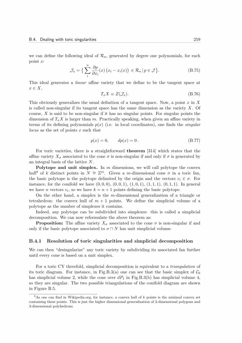
B.4. Dealing with toric singularities 259
we can define the following ideal of Rn, generated by degree one polynomials, for eachpoint x:
Jx =
n∑
i
∂p
∂xi(x)(xi − xi(x)
)∈ Rn | p ∈ J
. (B.75)
This ideal generates a linear affine variety that we define to be the tangent space atx ∈ X,
TxX ≡ Z(Jx). (B.76)
This obviously generalizes the usual definition of a tangent space. Now, a point x in Xis called non-singular if its tangent space has the same dimension as the variety X. Ofcourse, X is said to be non-singular if it has no singular points. For singular points thedimension of TxX is larger than m. Practically speaking, when given an affine variety interms of its defining polynomials p(x) (i.e. in local coordinates), one finds the singularlocus as the set of points x such that
p(x) = 0, dp(x) = 0 . (B.77)
For toric varieties, there is a straightforward theorem [314] which states that theaffine variety Xσ associated to the cone σ is non-singular if and only if σ is generated byan integral basis of the lattice N .
Polytope and unit simplex. In m dimensions, we will call polytope the convexhull8 of k distinct points in N ∼= Z
m. Given a m-dimensional cone σ in a toric fan,the basic polytope is the polytope delimited by the origin and the vectors vi ∈ σ. Forinstance, for the conifold we have (0, 0, 0), (0, 0, 1), (1, 0, 1), (1, 1, 1), (0, 1, 1). In generalwe have n vectors vi, so we have k = n+ 1 points defining the basic polytope.
On the other hand, a simplex is the m-dimensional generalization of a triangle ortetrahedron: the convex hull of m + 1 points. We define the simplicial volume of apolytope as the number of simplexes it contains.
Indeed, any polytope can be subdivided into simplexes: this is called a simplicialdecomposition. We can now reformulate the above theorem as:
Proposition: The affine variety Xσ associated to the cone σ is non-singular if andonly if the basic polytope associated to σ ∩N has unit simplicial volume.
B.4.1 Resolution of toric singularities and simplicial decomposition
We can then “desingularize” any toric variety by subdividing its associated fan furtheruntil every cone is based on a unit simplex.
For a toric CY threefold, simplicial decomposition is equivalent to a triangulation ofits toric diagram. For instance, in Fig.B.3(a) one can see that the basic simplex of C0has simplicial volume 2, while the cone over dP1 in Fig.B.3(b) has simplicial volume 4,so they are singular. The two possible triangulations of the conifold diagram are shownin Figure B.5.
8As one can find in Wikipedia.org, for instance, a convex hull of k points is the minimal convex setcontaining these points. This is just the higher dimensional generalization of 2-dimensional polygons and3-dimensional polyhedrons.
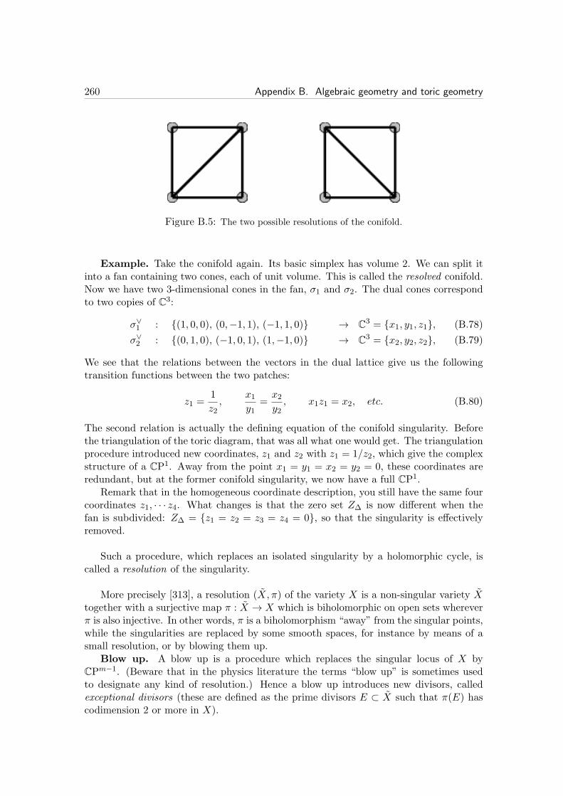
260 Appendix B. Algebraic geometry and toric geometry
Figure B.5: The two possible resolutions of the conifold.
Example. Take the conifold again. Its basic simplex has volume 2. We can split itinto a fan containing two cones, each of unit volume. This is called the resolved conifold.Now we have two 3-dimensional cones in the fan, σ1 and σ2. The dual cones correspondto two copies of C3:
σ∨1 : (1, 0, 0), (0,−1, 1), (−1, 1, 0) → C3 = x1, y1, z1, (B.78)
σ∨2 : (0, 1, 0), (−1, 0, 1), (1,−1, 0) → C3 = x2, y2, z2, (B.79)
We see that the relations between the vectors in the dual lattice give us the followingtransition functions between the two patches:
z1 =1
z2,
x1y1
=x2y2, x1z1 = x2, etc. (B.80)
The second relation is actually the defining equation of the conifold singularity. Beforethe triangulation of the toric diagram, that was all what one would get. The triangulationprocedure introduced new coordinates, z1 and z2 with z1 = 1/z2, which give the complexstructure of a CP1. Away from the point x1 = y1 = x2 = y2 = 0, these coordinates areredundant, but at the former conifold singularity, we now have a full CP1.
Remark that in the homogeneous coordinate description, you still have the same fourcoordinates z1, · · · z4. What changes is that the zero set Z∆ is now different when thefan is subdivided: Z∆ = z1 = z2 = z3 = z4 = 0, so that the singularity is effectivelyremoved.
Such a procedure, which replaces an isolated singularity by a holomorphic cycle, iscalled a resolution of the singularity.
More precisely [313], a resolution (X, π) of the variety X is a non-singular variety Xtogether with a surjective map π : X → X which is biholomorphic on open sets whereverπ is also injective. In other words, π is a biholomorphism “away” from the singular points,while the singularities are replaced by some smooth spaces, for instance by means of asmall resolution, or by blowing them up.
Blow up. A blow up is a procedure which replaces the singular locus of X byCPm−1. (Beware that in the physics literature the terms “blow up” is sometimes usedto designate any kind of resolution.) Hence a blow up introduces new divisors, calledexceptional divisors (these are defined as the prime divisors E ⊂ X such that π(E) hascodimension 2 or more in X).
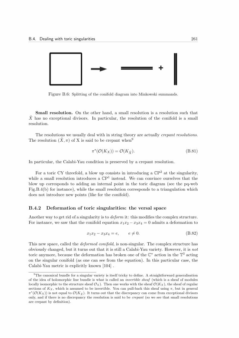
B.4. Dealing with toric singularities 261
Figure B.6: Splitting of the conifold diagram into Minkowski summands.
Small resolution. On the other hand, a small resolution is a resolution such thatX has no exceptional divisors. In particular, the resolution of the conifold is a smallresolution.
The resolutions we usually deal with in string theory are actually crepant resolutions.The resolution (X, π) of X is said to be crepant when9
π∗(O(KX)) = O(KX). (B.81)
In particular, the Calabi-Yau condition is preserved by a crepant resolution.
For a toric CY threefold, a blow up consists in introducing a CP2 at the singularity,while a small resolution introduces a CP1 instead. We can convince ourselves that theblow up corresponds to adding an internal point in the toric diagram (see the pq-webFig.B.4(b) for instance), while the small resolution corresponds to a triangulation whichdoes not introduce new points (like for the conifold).
B.4.2 Deformation of toric singularities: the versal space
Another way to get rid of a singularity is to deform it: this modifies the complex structure.For instance, we saw that the conifold equation x1x2−x3x4 = 0 admits a deformation to
x1x2 − x3x4 = e, e 6= 0. (B.82)
This new space, called the deformed conifold, is non-singular. The complex structure hasobviously changed, but it turns out that it is still a Calabi-Yau variety. However, it is nottoric anymore, because the deformation has broken one of the C
∗ action in the T3 acting
on the singular conifold (as one can see from the equation). In this particular case, theCalabi-Yau metric is explicitly known [104] .
9The canonical bundle for a singular variety is itself tricky to define. A straightforward generalisationof the idea of holomorphic line bundle is what is called an invertible sheaf (which is a sheaf of moduleslocally isomorphic to the structure sheaf OX). Then one works with the sheaf O(KX), the sheaf of regularsections of KX , which is assumed to be invertible. You can pull-back this sheaf using π, but in generalπ∗(O(KX)) is not equal to O(KX). It turns out that the discrepancy can come from exceptional divisorsonly, and if there is no discrepancy the resolution is said to be crepant (so we see that small resolutionsare crepant by definition).
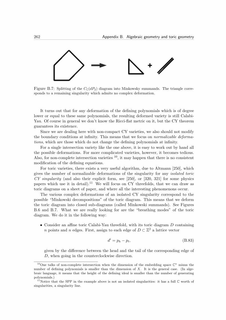
262 Appendix B. Algebraic geometry and toric geometry
Figure B.7: Splitting of the CC(dP2) diagram into Minkowsky summands. The triangle corre-sponds to a remaining singularity which admits no complex deformation.
It turns out that for any deformation of the defining polynomials which is of degreelower or equal to these same polynomials, the resulting deformed variety is still Calabi-Yau. Of course in general we don’t know the Ricci-flat metric on it, but the CY theoremguarantees its existence.
Since we are dealing here with non-compact CY varieties, we also should not modifythe boundary conditions at infinity. This means that we focus on normalizable deforma-tions, which are those which do not change the defining polynomials at infinity.
For a single intersection variety like the one above, it is easy to work out by hand allthe possible deformations. For more complicated varieties, however, it becomes tedious.Also, for non-complete intersection varieties 10, it may happen that there is no consistentmodification of the defining equations.
For toric varieties, there exists a very useful algorithm, due to Altmann [250], whichgives the number of normalizable deformations of the singularity for any isolated toricCY singularity (and also their explicit form, see [250], or [320, 321] for some physicspapers which use it in detail).11 We will focus on CY threefolds, that we can draw astoric diagrams on a sheet of paper, and where all the interesting phenomenons occur.
The various complex deformations of an isolated CY singularity correspond to thepossible “Minkowski decompositions” of the toric diagram. This means that we deformthe toric diagram into closed sub-diagrams (called Minkowski summands). See FiguresB.6 and B.7. What we are really looking for are the “breathing modes” of the toricdiagram. We do it in the following way:
• Consider an affine toric Calabi-Yau threefold, with its toric diagram D containingn points and n edges. First, assign to each edge of D ⊂ Z
2 a lattice vector
di = ph − pt, (B.83)
given by the difference between the head and the tail of the corresponding edge ofD, when going in the counterclockwise direction.
10One talks of non-complete intersection when the dimension of the embedding space Cn minus the
number of defining polynomials is smaller than the dimension of X. It is the general case. (In alge-braic language, it means that the height of the defining ideal is smaller than the number of generatingpolynomials.)
11Notice that the SPP in the example above is not an isolated singularities: it has a full C worth ofsingularities, a singularity line.

B.5. Toric geometry 2: Gauged linear sigma-model 263
• Define the vector space
V (D) =(t1, · · · , tn) |
n∑
i
tidi = 0
. (B.84)
This vector space, including the trivial (t, t, t, t) component, is obviously of dimen-sion n−2. Ignoring the trivial rescaling, this is the linearized space of deformationsof X, of dimension n − 3. The deformation could be obstructed at second order,however.
• The versal 12 space of complex deformations of X is defined by the following idealof C[t1, · · · , tn]:
J =(
pk ≡n∑
i
(ti)kdi | k ∈ Z>0
)
. (B.85)
Actually this ideal is generated by the finite set of polynomials p1, · · · , pK , whereK is the maximum of the lattice width of the minimal pair of strips containing D[250].
This whole procedure amounts to find the Minkowski summands of the diagram D.In term of the dual pq-web, it corresponds to splitting the pq-web into sub-webs inequilibrium (i.e. the external legs must still sum to zero). For instance, you can see thatthe diagram in Fig.B.3(b) admits no Minkowski decomposition. This means that thedP1 singularity cannot be deformed: although its linear space of deformations (B.84) hasdimension one, there is an obstruction at second order.
Example. Consider the conifold, whose diagram is just a square. We have thefollowing edge vectors:
d1 = (1, 0), d2 = (0, 1), d3 = (−1, 0), d4 = (0,−1) . (B.86)
The linear space of deformation is simply generated by (t1, t2, t1, t2). There is no higherorder obstruction so the versal space boils down to the linear space
Spec(C[t]) = C , (B.87)
corresponding to the freedom of adding a constant term e in (B.82).
B.5 Toric geometry 2: Gauged linear sigma-model
There is an alternative, complementary approach to toric varieties, which does not directlyrely on algebraic geometry, but rather deals with the symplectic or (more precisely) Kahlerproperties of our varieties.
The idea is to split the quotient by (C∗)n−m in (B.37) into two steps. Since
C∗ ∼= U(1)× R>0, (B.88)
12“Versal space” means that all the possible deformations are there, but that the same deformationmight appear several times (if it appear only once we would have a “universal” space of deformation, thatis what happens for compact Calabi-Yau varieties, whose complex moduli space has a simpler topology.See [313].).

264 Appendix B. Algebraic geometry and toric geometry
we will first fix some “point” t ∈ R>0 (and t → 0 will correspond to a singular limit forthe toric variety), and secondly we will divide by the U(1) action (which is the gaugegroup, in the physics parlance). Such a procedure is well defined because we have a welldefined Kahler form on the parent space C
n. It is called a Kahler quotient of Cn.
B.5.1 Kahler quotient and moment maps
Before exploring the “physics”, let us briefly explain what is a Kahler quotient mathe-matically. We will focus on the quotient of Cn by an abelian group. The group G = U(1)r
(r = n−m) acts on Cn as (compare to (B.43))
U(1)r : Cn → Cn : (zi) 7→ (ei
∑
a ξaQai zi), (B.89)
where ξ = (ξ1, · · · , ξr) are element of the Lie algebra g = u(1)r ∼= Rr of the gauge group.
The action of g is then
ξ · F (z) =(i∑
i
∑
a
ξaQai zi
∂
∂zi+ c.c.)F (z). (B.90)
The complex conjugate is necessary to make it a real action.Definition: Given a Kahler manifold with Kahler 2-form ω, a moment map µ for
the group action of G on Cn is an element of the dual Lie algebra, g∗, such that
d〈µ, ξ〉 ≡ d(µaξa) = iξω, (B.91)
where here iξ denote the interior product with the vector ξ appearing on the r.h.s. of(B.90).
You can easily show that, in our case, the Kahler manifold being simply Cn with the
canonical Kahler formω = −i
∑
i
dzi ∧ dzi , (B.92)
the moment maps are
µa =∑
i
Qai |zi|2 − ta, (B.93)
where the ta are integration constants. Then, the Kahler quotient proceeds as follows:
• Set µa = 0, i.e.∑
i
Qai |zi|2 = ta ∀a, (B.94)
This is called a restriction to a level set at level t. The parameters ta could be setto zero, as we will see.
• The second step is to quotient by the compact gauge group U(1)r, whose actionwas defined in (B.89).
The first step defines a lower-dimensional real algebraic submanifold in the spaceRn≥0 spanned by the |zi|’s. Then the second step tells us which subgroup U(1)m of the
U(1)n ⊂ Cn torus must be fibered at each point to produce the final m-dimensional
variety.

B.5. Toric geometry 2: Gauged linear sigma-model 265
B.5.2 The GLSM story
If your are familiar with supersymmetric theories (or you have read the introductioncarefully), the above must have looked like known territory. The restriction to a level setis simply the imposition of the D-term constraints in some abelian gauge theory, whilethe second steps corresponds to fixing the gauge freedom (restricting to gauge orbits).
Hence, we can see toric varieties as the moduli space of vacua of a “gauged linearsigma-model” (GLSM). We have n chiral fields whose scalar component are the zi’s, andthey are charged under the gauge group as
z1 · · · zn FI
U(1)1 Q11 · · · Q1
n t1
.... . .
...U(1)r Qr1 · · · Qrn tr
Because the gauge group is U(1)r, there are possible Fayet-Iliopoulos (FI) parameters ta
in the D-terms conditions (B.94). This was first realised by Witten in [322], where heused a 2-dimensional GLSM as an auxiliary device to find 2-dimensional CFTs. Here theauxiliary theory is four dimensional (the main difference with respect to [322] being thatthe FI parameters are real), and its infrared corresponds to a Calabi-Yau “as probed byD3-branes”13.
Examples. Consider the GLSM with a single U(1) and four fields with the followingcharges:
z1 z2 z3 z4U(1) p p −p+ q −p− q
and no FI term. The resulting toric Calabi-Yau singularity is a real cone over a real 5-dimensional Sasaki-Einstein14 space called Y p,q [323]. This family of toric CY singularitieshas received a lot a attention in the physics litterature during the last years, because thecorresponding Ricci-flat metrics are known explicitly [105], which is a rather spectacularfeat and allowed for some new checks of the AdS/CFT correspondence.
B.5.3 Toric varieties as torus fibration of polytopes
An affine toric variety X can be visualized quite simply as a torus fibration over a polytope∆:
U(1)m → XµH−→ ∆ (B.95)
Indeed, the toric variety X has an isometry group
H = U(1)m =U(1)n
U(1)r, (B.96)
and there is a moment map µH on X associated to this H. This moment map is preciselythe map which projects out the U(1)m fibers in the exact short sequence (B.95) [323].
13You should not take this analogy too seriously: the GLSM is an auxiliary construction, like the fan,there is a priori no real physics there.
14Sasaki basically means that the real 6-dimensional cone is Kahler, while the Einstein condition on the5-dimensional base metric implies the Ricci-flatness of the cone. Hence a SE manifold of real dimension2n− 1 is the real base of a CY cone of complex dimension n.
266 Appendix B. Algebraic geometry and toric geometry
For cones (ta = 0), the polytope is precisely the toric cone σ for X. Given the chargevectors Qa, one can construct several σ’s such that
σ =Span((vi) ∈ N ∼= Z
m) |∑
i
Qai vi ∀a. (B.97)
All these σ are related to each other by Sl(m,Z) transformations. Consider, for instance,taking an orthogonal basis of Zm for the first m lattice vectors vi (corresponding to thefirst m homogeneous coordinates). The remaining vectors of σ follow from (B.44). Thischoice of lattice basis vectors corresponds to a choice of subgroup for
U(1)m ⊂ U(1)n . (B.98)
This is simply because we made a choice about which of the homogeneous coordinates(zi) are the “dependent” ones. Here we chose the variables (zm+1, · · · , zn) to be functionsof the (z1, · · · , zm). More precisely, the modulus are fixed by the D-terms (B.94), whilethe phases of (zm+1, · · · , zn) are redundant U(1)r degrees of freedom that we can gaugefix.
Then we see explicitly that the affine toric variety is realized as a U(1)m fibrationof σ ⊂ NR. In the bulk, the real torus Tm ∼= U(1)m is non-degenerate, while on theintersection of the hyperplane (vj = 0, ∀j ∈ I ⊂ (1, · · ·m)) with the cone σ, there is adegeneration of the (#I)-torus (T 1
j1×· · ·×T 1
(#I)). At the tip of σ the whole torus shrinksto zero, and we have a singularity.
Example. Take the conifold again. We have Q = (1,−1, 1,−1). If we take a basis ofZ3 as (0, 0, 1), (0, 1, 1) and (1, 1, 1), we must have that the fourth vector in σ be (1, 0, 1).
On the other hand, if we take the orthogonal basis for the lattice, σ is generated by
(1, 0, 0), (0, 1, 0), (0, 0, 1), (1,−1, 1). (B.99)
We see that the first σ is obtained from the second by the Sl(3,Z) transformation
0 1 10 0 11 1 1
. (B.100)
When ta 6= 0 for some a’s, we have a (possibly partially) resolved singularity. Fromthe polytope point of view, the resolution amounts to “chopping off” the tip of σ, sincewe cannot reach the point z1 = · · · = zn = 0 anymore. As an aside, let us note theinteresting relation between the parameter ta and the period of the Kahler form on thecorresponding 2-cycle Ca (in the case of a small resolution by a CP1) [288] :
∫
Caω = ta. (B.101)
So the FI parameters in the GLSM really map to the “Kahler volumes” of the resolvingcycles.
The GLSM perspective is very interesting in order to explore the topology of toric va-rieties, and it is “easier” because more explicit. One can easily visualize toric divisors andcompute their intersections using the GLSM. Nice reviews exist in the physics literatureon this part of the story. See in particular: [288], [324], and the chapter 7 of [325].
Appendix C
N = 1 renormalization group andSeiberg duality
C.1 RG equations for N = 1 gauge theories
Let us briefly recall some results on the renormalization ofN = 1 gauge theories. Considera theory with a gauge groupling g and some superpotential couplings hn. We havea superpotential W =
∑
n hnOn for some operators On polynomial in the UV chiralsuperfields of the theory.
C.1.1 Superpotential couplings
It is well known that the holomorphic superpotential couplings hn are not renormalized[131]. However, the physical coupling do suffer wave-function renormalisation. Considerfor instance the superpotential term
W ⊃ hO = h∏
i
(Φi)di (C.1)
where the operator O has a classical dimension dO =∑
i di. We define the dimensionlessphysical coupling as
h = µdO−3
(∏
i
Z−di2
i
)
h (C.2)
where µ is the renormalisation scale and Zi is the wave-renormalisation factor of the fieldΦi
1. Consequently, the quantum beta function for h is
β(h) = µ∂h
∂µ=
(
dO +1
2
∑
i
diγi − 3
)
h . (C.3)
We use the following definition for the anomalous dimension of a field φ:
γφ = −µ ∂
∂µlnZφ . (C.4)
1Note that Φ =√ZΦ0, with Φ and Φ0 the renormalised and bare quantities, respectively.
267
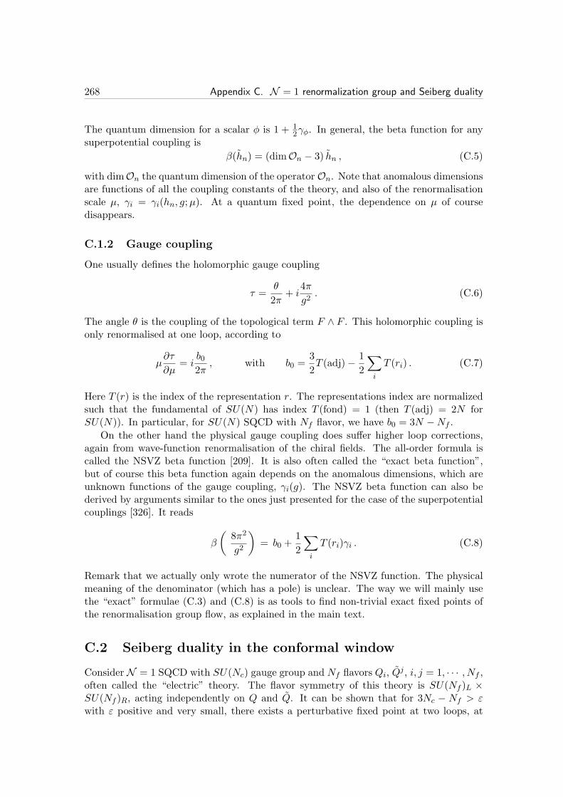
268 Appendix C. N = 1 renormalization group and Seiberg duality
The quantum dimension for a scalar φ is 1 + 12γφ. In general, the beta function for any
superpotential coupling is
β(hn) = (dimOn − 3) hn , (C.5)
with dimOn the quantum dimension of the operatorOn. Note that anomalous dimensionsare functions of all the coupling constants of the theory, and also of the renormalisationscale µ, γi = γi(hn, g;µ). At a quantum fixed point, the dependence on µ of coursedisappears.
C.1.2 Gauge coupling
One usually defines the holomorphic gauge coupling
τ =θ
2π+ i
4π
g2. (C.6)
The angle θ is the coupling of the topological term F ∧ F . This holomorphic coupling isonly renormalised at one loop, according to
µ∂τ
∂µ= i
b02π
, with b0 =3
2T (adj)− 1
2
∑
i
T (ri) . (C.7)
Here T (r) is the index of the representation r. The representations index are normalizedsuch that the fundamental of SU(N) has index T (fond) = 1 (then T (adj) = 2N forSU(N)). In particular, for SU(N) SQCD with Nf flavor, we have b0 = 3N −Nf .
On the other hand the physical gauge coupling does suffer higher loop corrections,again from wave-function renormalisation of the chiral fields. The all-order formula iscalled the NSVZ beta function [209]. It is also often called the “exact beta function”,but of course this beta function again depends on the anomalous dimensions, which areunknown functions of the gauge coupling, γi(g). The NSVZ beta function can also bederived by arguments similar to the ones just presented for the case of the superpotentialcouplings [326]. It reads
β
(8π2
g2
)
= b0 +1
2
∑
i
T (ri)γi . (C.8)
Remark that we actually only wrote the numerator of the NSVZ function. The physicalmeaning of the denominator (which has a pole) is unclear. The way we will mainly usethe “exact” formulae (C.3) and (C.8) is as tools to find non-trivial exact fixed points ofthe renormalisation group flow, as explained in the main text.
C.2 Seiberg duality in the conformal window
Consider N = 1 SQCD with SU(Nc) gauge group and Nf flavors Qi, Qj , i, j = 1, · · · , Nf ,
often called the “electric” theory. The flavor symmetry of this theory is SU(Nf )L ×SU(Nf )R, acting independently on Q and Q. It can be shown that for 3Nc − Nf > εwith ε positive and very small, there exists a perturbative fixed point at two loops, at

C.3. Seiberg duality with a quartic superpotential 269
a critical value g = g∗ ∼ εN [83]. It was famously conjectured by Seiberg [83] that this
fixed point is in fact exact and that it exist for any Nf in the range
3
2Nc < Nf < 3Nc . (C.9)
This range is called the conformal window of SQCD. Using the NSVZ beta function, wesee that the anomalous dimension γ0 of the quarks Q, Q must be γ0 = (Nf − 3Nc)/Nf
at the fixed point, and that the superconformal R-charge is
R(Q) = R(Q) =Nf −Nc
Nf. (C.10)
As we decrease Nf , the anomalous dimensions get large and the interacting fixed pointbecomes strongly coupled. Let us call this SCFT the “electric SCFT”.
Consider also another N = 1 theory with SU(Nf −Nc) gauge group and Nf flavorsqi, q
j , j = 1, · · · , Nf , together with a gauge singlet field M ij transforming in the (Nf , Nf )
of SU(Nf )L × SU(Nf )R, and a superpotential
W = y qiMij qj , (C.11)
which preserves the SU(Nf )L × SU(Nf )R flavor group. This is called the “magnetic”theory. Using the exact beta functions for the gauge coupling g and the superpotentialcoupling y, one can show that such theory might indeed posses an exact fixed point aslong as the parameters Nf and Nc satisfy (C.9). First notice that if y = 0 we are at theSQCD fixed point with Nc = Nf − Nc, with γ0 = (3Nc − 2Nf )/Nf for the quarks q, q,while the gauge singlet M is decoupled and must have dimension 1. Hence the operatorMqq is a relevant deformation of the SQCD fixed point. For any small y the theory thenflows away from this fixed point, and can reach another fixed point where the anomalousdimension for M is increased to γM = (4Nf − 6Nc)/Nf . This isolated fixed point atnon-trivial values of g and y is called the “magnetic SCFT”.
The Seiberg duality conjecture is that the electric and magnetic SCFT are preciselyequivalent. For reviews of the beautiful consistency checks one can make of this conjecture,we refer to [131]. It is interesting to note that at the magnetic fixed point the fieldsM i
j can
be identified with the SQCD mesons QiQj in the electric SCFT; for instance it is easy tocheck they both have the same quantum dimension, ∆(M) = ∆(QQ) = 3(Nf −Nc)/Nf .For this reason the field M is often called the “dual meson”.
Seiberg duality is also often stated as “the IR limits of the electric and magnetictheories are equivalent”; this formulation is then correct even for Nf <
32Nc, when SQCD
does not reach a fixed point but becomes dual to an IR free magnetic theory in the IR[83].
C.3 Seiberg duality with a quartic superpotential
The N = 1 Seiberg duality as presented in the previous section is a duality between twoisolated fixed points. In that respect it is quite different from the S-duality of N = 4,

270 Appendix C. N = 1 renormalization group and Seiberg duality
for instance, which acts on a continuous line of fixed points. An interesting extension ofSeiberg duality is obtained by adding a quartic superpotential
W = h(QiQj)(QjQ
i) (C.12)
to the electric SCFT. For h small, we can compute the beta function using the anomalousdimensions of the electric SCFT. We have three cases:
• Nf = 2Nc. This case was discussed in the main text, in section 4.1.4. The betafunction for g and for h are proportional, so there is a line of fixed points.
• Nf > 2Nc. We have R(Q) > 12 at the electric SCFT. The quartic superpotential
(C.12) is then irrelevant, as it would be classically.
• Nf < 2Nc. In this case we have R(Q) < 12 in the electric SCFT, so the quartic
superpotential is relevant. We can then use it to perturb the fixed point and starta non-trivial RG flow.
The third case is the most interesting: we see an instance of a superpotential which isclassically irrelevant but becomes relevant at strong coupling (near the electric SCFTfixed point).
The Seiberg dual theory has a SU(Nf − Nc) gauge group, Nf dual quarks and thedual mesons, with superpotential
W = y qiMij qj + hM i
jMji . (C.13)
Note that the coupling h looks like a mass term. However, we must check its RG runningas in the case of the electric theory. For Nf = 2Nc the coupling h is marginal, hence wehave a line of fixed points, as expected from the electric theory. When Nf > 2Nc thecoupling h is irrelevant, while for Nf < 2Nc it is relevant.
If we integrate out the field M , we obtain the effective superpotential
W = h′ (qiqj)(qj q
i) , (C.14)
with h′ ∼ y2/m, so we see that the electric and magnetic theories have the same super-potential. However, when h is a relevant coupling, the dual h′ is an irrelevant coupling,and vice-versa. As carefully explained in [85], when Nf < 2Nc Seiberg duality relates theRG flow away from the electric SCFT, as h grows from 0 to infinity, to the dual RG flowfrom h′ =∞ to 0, towards the magnetic SCFT.
In the case Nf = 2Nc, both electric and magnetic theories have an SU(Nc) gaugegroup and a marginal quartic superpotential, so they are really self-similar, and Seibergduality is most similar to an S-duality, relating strong to weak coupling h on the line offixed points.
Seiberg duality for SQCD with a quartic superpotential can be derived from a carefulanalysis of N = 2 SQCD, as was done in [155]; in that early reference, however, theymissed the fact that the quartic superpotential can actually turn out to be relevant inthe far IR, which is quite important to understand the famous duality cascade of [118].

Appendix D
Spherical coordinates on R6
In this Appendix we discuss some coordinates on S5 and the associated harmonic func-tions (which we present for completeness although we will not need them in any detail).We then go on to derive the equation (4.46) of Chapter 4.
D.1 Spherical polar coordinates on R6
We consider the following spherical polar coordinates on R6:
x1 = r cos θ1
x2 = r sin θ1 cos θ2
x3 = r sin θ1 sin θ2 cos θ3
x4 = r sin θ1 sin θ2 sin θ3 cos θ4
x5 = r sin θ1 sin θ2 sin θ3 sin θ4 cosϕ
x6 = r sin θ1 sin θ2 sin θ3 sin θ4 sinϕ
(D.1)
where θj ∈ [0, π] and ϕ ∈ [0, 2π). The volume form is then
r5dr∧ dvol(S5) = r5dr∧ (sin θ1)4(sin θ2)3(sin θ3)2 sin θ4dθ1 ∧ dθ2 ∧ dθ3 ∧ dθ4 ∧ dϕ . (D.2)
The Laplacian on R6 is
∆R6 =1
r5∂rr
5∂r +1
r2∆S5 , (D.3)
with the angular Laplacian on S5 that reads
∆S5 = (∂θ1 + 4 cot θ1)∂θ1 +1
(sin θ1)2(∂θ2 + 3 cot θ2)∂θ2 +
1
(sin θ1 sin θ2)2(∂θ3 + 2 cot θ3)∂θ3+
+1
(sin θ1 sin θ2 sin θ3)2(∂θ4 + cot θ4)∂θ4 +
1
(sin θ1 sin θ2 sin θ3 sin θ4)2∂2ϕ
(D.4)
271
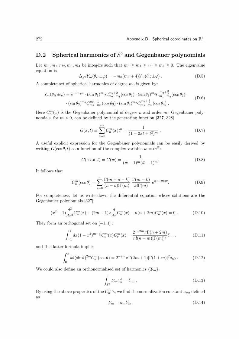
272 Appendix D. Spherical coordinates on R6
D.2 Spherical harmonics of S5 and Gegenbauer polynomials
Let m0,m1,m2,m3,m4 be integers such that m0 ≥ m1 ≥ · · · ≥ m4 ≥ 0. The eigenvalueequation is
∆S5Ym(θi;±ϕ) = −m0(m0 + 4)Ym(θi;±ϕ) . (D.5)
A complete set of spherical harmonics of degree m0 is given by:
Ym(θi;±ϕ) = e±im4ϕ · (sin θ1)m1Cm1+2m0−m1
(cos θ1) · (sin θ2)m2Cm2+
32
m1−m2(cos θ2)·
· (sin θ3)m3Cm3+1m2−m3
(cos θ3) · (sin θ4)m4Cm4+
12
m3−m4(cos θ4) .
(D.6)
Here Cmn (x) is the Gegenbauer polynomial of degree n and order m. Gegenbauer poly-nomials, for m > 0, can be defined by the generating function [327, 328]
G(x, t) ≡∞∑
n=0
Cmn (x)tn =1
(1− 2xt+ t2)m. (D.7)
A useful explicit expression for the Gegenbauer polynomials can be easily derived bywriting G(cos θ, t) as a function of the complex variable w = teiθ:
G(cos θ, t) = G(w) =1
(w − 1)m(w − 1)m. (D.8)
It follows that
Cmn (cos θ) =n∑
k=0
Γ(m+ n− k)(n− k)!Γ(m)
Γ(m− k)k!Γ(m)
ei(n−2k)θ. (D.9)
For completeness, let us write down the differential equation whose solutions are theGegenbauer polynomials [327]:
(x2 − 1)d2
dx2Cmn (x) + (2m+ 1)x
d
dxCmn (x)− n(n+ 2m)Cmn (x) = 0 . (D.10)
They form an orthogonal set on [−1, 1] :∫ 1
−1dx(1− x2)m− 1
2Cmn (x)Cmr (x) =21−2mπΓ(n+ 2m)
n!(n+m)[Γ(m)]2δnr , (D.11)
and this latter formula implies∫ π
0dθ(sin θ)2mCmn (cos θ) = 2−2mπΓ(2m+ 1)[Γ(1 +m)]2δn0 . (D.12)
We could also define an orthonormalised set of harmonics Ym,∫
S5
YmY∗n = δnm. (D.13)
By using the above properties of the Cmn ’s, we find the normalization constant am, definedas
Ym = amYm, (D.14)

D.3. Solving for the warp factor of a 2 stacks system 273
to be given by
am =
(
(m0 −m1)! · · · (m3 −m4)![Γ(2 +m1) · · ·Γ(12 +m4)]2(2 +m0) · · · (12 +m3)
2π5 4−3−(m1+···+m4)Γ(4 +m0 +m1) · · ·Γ(1 +m3 +m4)
) 12
.
(D.15)
D.3 Solving for the warp factor of a 2 stacks system
Consider a stack of N − N ′ D3-branes at (xi) = 0, and a stack of N ′ D3-branes at(xi) = (s, 0, · · · , 0). The warp factor equation,
∆6h = −2κ2τ3((N −N ′)δ6(x) +N ′δ6(x− s)
), (D.16)
can be expanded in harmonics. In this particular case, we have
δ6(x− s) = δ(x1 − s)δ(x2) · · · δ(x6) = δ(r − s)r5
∑
m0
(m0 + 2)
2π3Ym0(θ1), (D.17)
with Ym0(θ1) = C2m0
(cos θ1). Then, expanding as
h(r, θ1) =∑
m0
Hm0(r) Ym0(θ1), (D.18)
we have the radial equations
[
∆r −m0(m0 + 4)
r2
]
Hm0(r) = −4R4(N−N ′)
δ(r)
r5δm0,0 − 4R4
N ′
(m0 + 2)
2
δ(r − s)r5
, (D.19)
where R4N = 4πNα′2gs. It is then straightforward to derive (for r > s)
h(r, θ1) =R4N
r4
(
1 +N ′
N
∞∑
m0=1
(s
r
)m0
Ym0(θ1)
)
. (D.20)
This is equation (4.46).


Appendix E
Seiberg-Witten theory
Seiberg-Witten theory is the theory which provides the full non-perturbative solution forN = 2 supersymmtric gauge theories in four dimensions, in the sense that it gives theexact low energy Wilsonian action. In this Appendix we will intoduce the SW formalismfrom scratch, emphasizing the aspects which are important to understand the work pre-sented in Chapter 6. We first introduce the SW formalism in the field theory language,and later mention the beautiful relationship between SW theory and M-theory. We focuson the case of the special unitary gauge group SU(N).
E.1 N = 2 vector mutliplet and the effective action
The N = 2 four dimensional vector multiplet contains a vector, two Weyl fermionsand one complex scalar, all in the adjoint representation of the gauge group. In orderto construct a supersymmetric action, it is useful to introduce an N = 2 superspace
(x, θ, θ, θ,¯θ), where the Grasmannians θ,
¯θ extend the usual N = 1 superspace. The
N = 2 vector superfield can be expanded in term of N = 1 chiral superfields Φ andWα = −1
4D2DαV , as [329, 330]
Ψ(y, θ, θ) = Φ(y, θ) +√2θαWα(y, θ) + θθΨ(D)(y, θ) , (E.1)
where we have used the chiral coordinate yµ = xµ + iθσµθ + iθσµ¯θ, and
Ψ(D)(y, θ) = Φ†(y − iθσµθ, θ, θ)e2V (y−iθσµθ,θ,θ)∣∣θθ. (E.2)
The most general action for the N = 2 vector superfield is
L =1
4πIm
∫
d2θd2θF(Ψ) , (E.3)
where F is any holomorphic function of Ψ, called the prepotential. It is the holomorphic-ity property of the prepotential which ultimately allows to compute the effective actionexactly in any vacuum. In the UV, the theory is defined by
F(Ψ) =τ
2Ψ2 , (E.4)
275
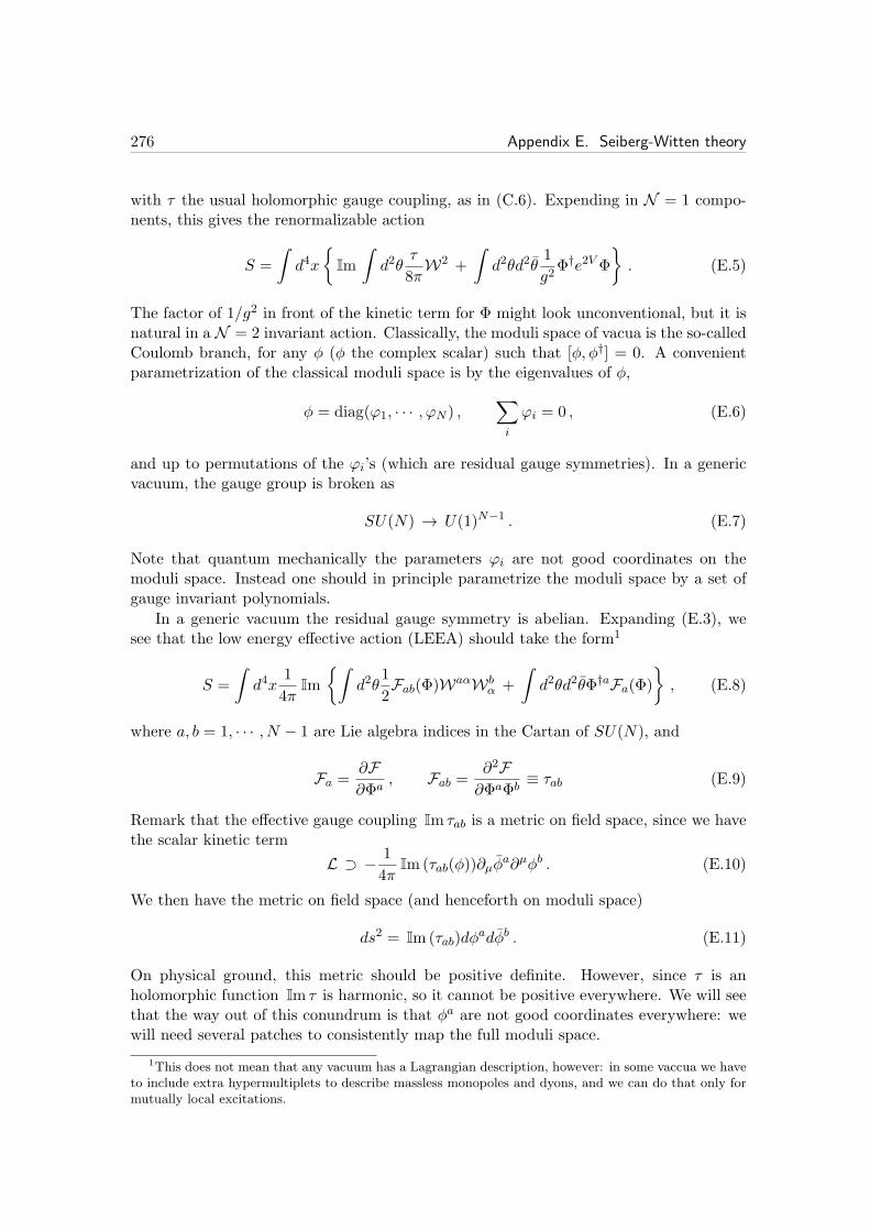
276 Appendix E. Seiberg-Witten theory
with τ the usual holomorphic gauge coupling, as in (C.6). Expending in N = 1 compo-nents, this gives the renormalizable action
S =
∫
d4x
Im
∫
d2θτ
8πW2 +
∫
d2θd2θ1
g2Φ†e2V Φ
. (E.5)
The factor of 1/g2 in front of the kinetic term for Φ might look unconventional, but it isnatural in a N = 2 invariant action. Classically, the moduli space of vacua is the so-calledCoulomb branch, for any φ (φ the complex scalar) such that [φ, φ†] = 0. A convenientparametrization of the classical moduli space is by the eigenvalues of φ,
φ = diag(ϕ1, · · · , ϕN ) ,∑
i
ϕi = 0 , (E.6)
and up to permutations of the ϕi’s (which are residual gauge symmetries). In a genericvacuum, the gauge group is broken as
SU(N) → U(1)N−1 . (E.7)
Note that quantum mechanically the parameters ϕi are not good coordinates on themoduli space. Instead one should in principle parametrize the moduli space by a set ofgauge invariant polynomials.
In a generic vacuum the residual gauge symmetry is abelian. Expanding (E.3), wesee that the low energy effective action (LEEA) should take the form1
S =
∫
d4x1
4πIm
∫
d2θ1
2Fab(Φ)WaαWb
α +
∫
d2θd2θΦ†aFa(Φ)
, (E.8)
where a, b = 1, · · · , N − 1 are Lie algebra indices in the Cartan of SU(N), and
Fa =∂F∂Φa
, Fab =∂2F∂ΦaΦb
≡ τab (E.9)
Remark that the effective gauge coupling Im τab is a metric on field space, since we havethe scalar kinetic term
L ⊃ − 1
4πIm(τab(φ))∂µφ
a∂µφb . (E.10)
We then have the metric on field space (and henceforth on moduli space)
ds2 = Im(τab)dφadφb . (E.11)
On physical ground, this metric should be positive definite. However, since τ is anholomorphic function Im τ is harmonic, so it cannot be positive everywhere. We will seethat the way out of this conundrum is that φa are not good coordinates everywhere: wewill need several patches to consistently map the full moduli space.
1This does not mean that any vacuum has a Lagrangian description, however: in some vaccua we haveto include extra hypermultiplets to describe massless monopoles and dyons, and we can do that only formutually local excitations.

E.2. Electric-magnetic duality 277
E.1.1 R-symmetry and the perturbative prepotential
Classically, the UV theory (E.5) has a R-symmetry U(1)R which assigns charge 0, 1 and2 to the vector, the fermions and the complex scalar, respectively. There is however achiral anomaly,
φ→ ei2αφ , θ → θ − 4Nα , (E.12)
which breaks U(1)R to Z4N . Moreover, the actual symmetry acting on the Coulombbranch is Z2M since φ has R-charge 2. We can easily compute the perturbative runningcoupling, by the following trick [331, 332]: since F ′′ = τ , the anomalous shift in the thetaangle can be written as
F ′′(e2iαφ)−F ′′(φ) = −4Nα
2π⇒ ∂3F
∂φ3=i
π
N
φ, (E.13)
where the implication is for α infinitesimal. Integrating the expression on the right, wehave
τpert = F ′′pert = −
2N
2πilnφ
Λ, with Λ = µe2πiτ(µ) , (E.14)
while the prepotential can be schematically written as
Fpert = −N
2πiφ2 ln
φ
Λ. (E.15)
This result is actually exact in perturbation theory [331]. However, non-perturbativeeffects will drastically change the result at strong coupling.
E.2 Electric-magnetic duality
Classical electric-magnetic duality for abelian gauge fields exchanges the field strengthwith its Hodge dual, F ↔ ∗F . Consequently, it exchanges electric and magnetic sources,or equation of motion (EOM) and Bianchi identity (BI)
d ∗ F = ∗je , dF = ∗jm with je ↔ jm . (E.16)
In the absence of sources, this is also a symmetry of the quantum theory. Formally, itcan be seen as a change of variable in the path integral. Suppose that we take F insteadof the gauge field A to be the dynamical field (the one we path integrate over). We cando that provided we also introduce a Lagrange multiplier AD which imposes the BI,
S =
∫
R3,1
−1
4F ∧ ∗F +
1
2AD ∧ dF
(E.17)
We can then perform the path integral over F . The equation of motion for F tells usthat ∗F = FD; plugging into the action, we have a new action2 which only depends onAD, through FD = dAD,
Sdual =
∫
R3,1
−1
4FD ∧ ∗FD
. (E.18)
2Recall that in Lorentzian signature the operator ∗ : Λ2 → Λ2 squares to −1 in four dimensions, soF = − ∗ FD.
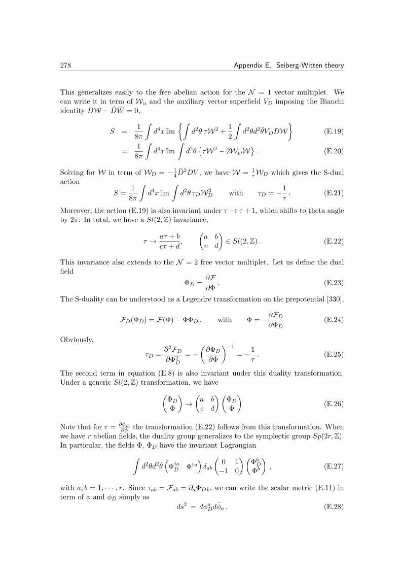
278 Appendix E. Seiberg-Witten theory
This generalizes easily to the free abelian action for the N = 1 vector multiplet. Wecan write it in term of Wα and the auxiliary vector superfield VD imposing the Bianchiidentity DW − DW = 0,
S =1
8π
∫
d4x Im
∫
d2θ τW2 +1
2
∫
d2θd2θVDDW
(E.19)
=1
8π
∫
d4x Im
∫
d2θτW2 − 2WDW
. (E.20)
Solving for W in term of WD = −14D
2DV , we have W = 1τWD which gives the S-dual
action
S =1
8π
∫
d4x Im
∫
d2θ τDW2D with τD = −1
τ. (E.21)
Moreover, the action (E.19) is also invariant under τ → τ +1, which shifts to theta angleby 2π. In total, we have a Sl(2,Z) invariance,
τ → aτ + b
cτ + d,
(a bc d
)
∈ Sl(2,Z) . (E.22)
This invariance also extends to the N = 2 free vector multiplet. Let us define the dualfield
ΦD =∂F∂Φ
. (E.23)
The S-duality can be understood as a Legendre transformation on the prepotential [330],
FD(ΦD) = F(Φ)− ΦΦD , with Φ = −∂FD∂ΦD
(E.24)
Obviously,
τD =∂2FD∂Φ2
D
= −(∂ΦD∂Φ
)−1
= −1
τ. (E.25)
The second term in equation (E.8) is also invariant under this duality transformation.Under a generic Sl(2,Z) transformation, we have
(ΦDΦ
)
→(a bc d
)(ΦDΦ
)
(E.26)
Note that for τ = ∂φD∂φ the transformation (E.22) follows from this transformation. When
we have r abelian fields, the duality group generalizes to the symplectic group Sp(2r,Z).In particular, the fields Φ, ΦD have the invariant Lagrangian
∫
d2θd2θ(
Φ†aD Φ†a
)
δab
(0 1−1 0
)(ΦbDΦb
)
, (E.27)
with a, b = 1, · · · , r. Since τab = Fab = ∂aΦD b, we can write the scalar metric (E.11) interm of φ and φD simply as
ds2 = dφaDdφa . (E.28)
E.3. Singularities and massless monopoles 279
The actual moduli spaceM is some complicated submanifold of complex dimension r inC2r ∼= φD, φ. Let us call z the coordinates on M, on some patch. The metric on the
moduli space in local coordinates reads
ds2 =∂φcD∂za
∂φbc∂zb
dzadzb . (E.29)
We have uncovered an important geometric structure, thanks to S-duality: the spaceC2r ∼= φD, φ is naturally seen as a Sp(2r,Z) bundle3,
Cr −→ C
2r π−→M . (E.30)
We can interpret the fields (φ(z), φD(z)) as a non-trivial section of this bundle: thefunctions (φaD, φ
a) on different patches are related by non-trivial Sp(2r,Z) duality trans-formations on overlaps.
E.3 Singularities and massless monopoles
The Wilsonian action for N = 2 SU(N) SYM,
S =
∫
d4x1
4πIm
∫
d2θ1
2τab(Φ)WaαWb
α +
∫
d2θd2θΦ†aΦ
aD
, (E.31)
describes N − 1 massless photons and their associated N = 2 superpartners. In the IRlimit any such vacuum is a trivial SCFT. This action is valid at low energy up to thescale of the first massive excitations. The lowest mass states will be the ones which areprotected by the N = 2 supersymmetry, saturating the BPS bound M ≥
√2|Z| which
follows from the N = 2 SUSY algebra. Remark that the possible massive excitationwe are talking about can be thought as ’t Hooft-Polyakov monopoles [293, 294] in thesemi-classical limit; they are some solitonic excitations of the non-linear SU(N) theory.Moreover, they fall into N = 2 hypermultiplets. Perturbatively, it is well known that|Z| = hφ/g2 for a ’t Hooft-Polyakov monopole of magnetic charge h when the θ anglevanishes4, while for generic complex coupling τ we have Z = hφτ , due to the Witteneffect [333], and Z = φ(hτ + q) for a dyon. The non-perturbative expression for Z in theN = 2 low energy theory can be deduced from the requirement of duality invariance; itis given by [154]
Z = haφaD + qaφa , (E.32)
with (φ, φD) = (φ(z0), φD(z0)) in the particular vacuum z = z0. The charges q and h arethe electric and magnetic charge of the state. Moreover, only the excitations with h andq relatively prime are stable [154]. The Sl(2N − 2,Z) duality symmetry acts as
(φDφ
)
→M
(φDφ
)
,
(hq
)
→ (M−1)t(hq
)
. (E.33)
3This is similar to the way symplectic bundles appear in classical mechanics. (φD, φ) are the analog ofthe canonical variables (p, q). The form dφ∧dφD−dφD ∧ φ is a symplectic form, and (E.28) a symplecticmetric.
4In our context this form of the mass is forced by the N = 2-preserving superpotential term ΦQQ,when coupling an hypermutliplet to the vector multiplet.
280 Appendix E. Seiberg-Witten theory
At isolated points on the moduli space, some BPS monopoles (generically some dyonsof a given charge (q, h)) might have a vanishing mass, M =
√2|Z| = 0. For instance if
φD = 0 in a vacuum the monopole of charge (1, 0) would be massless. In general, form,n ∈ Z relatively prime, if the particular combination mφD − nφ vanishes, the dyon ofcharge (h, q) = (m,n) becomes massless, as we can see from (E.32). At such a point themetric (E.29) is singular: we should include an hypermultiplet in the LEEA to accountfor the new massless degrees of freedom.
Singularities on the moduli space correspond to monodromies of the section (φD, φ).Suppose we have a hypermuliplet (written Q, Q in term of two N = 1 chiral superfields)with charge (h, q) = (0, 1) (electrically coupled) to a U(1) vector multiplet, which becomesmassless at z = z0. Suppose we can choose some local coordinates on the moduli spaceas z − z0 = φ. Since the U(1) gauge group is IR free in the presence of a masslesshypermultiplet, we can apply perturbation theory near φ = 0. One can easily show (forinstance, use (C.7) in Appendix C with b0 = −2Nf = −2 for a gauge group U(1)) thatthe gauge coupling goes like
τ(φ) =2
2πilnφ
Λ. (E.34)
We then have
φ = z − z0 , φD =1
πi(z − z0) ln
(z − z0)Λ
. (E.35)
When performing a rotation around z0, the function φ is invariant by assumption but φDchanges as φD → φD + 2φ. This is a monodromy, which we can also write as
(ΦDΦ
)
→M(0,1)
(ΦDΦ
)
, with M(0,1) =
(1 20 1
)
. (E.36)
From this result we can easily work out the monodromy matrix around a point whereany dyon of charge (m,n) becomes massless. If m and n are relatively prime, there existan Sl(2,Z) matrix S such that (m,n) = S(0, 1):
(m n
)= S
(0 1
), S =
(a bm n
)
, such that an− bm = 1 . (E.37)
The later equation in term of a and b is called Bezout’s identity, and it always has asolution. It follows that the monodromy matrix around the generic dyon is
M(m,n) = S−1M(0,1)S =
(1 + 2mn 2n2
−2m2 1− 2nm
)
. (E.38)
This result straightforwardly generalizes to a gauge group U(1)r and Sp(2r,Z)-valuedmonodromies.
There is also a weak coupling monodromies at infinity on the moduli space, whichis not of this type. A path circling around infinity is homotopic to (minus) the productof all the paths going once around a single strong coupling singularity. Hence the weakcoupling monodromy at infinity can be found by taking the product of all the srongcoupling monodromies. More details can be found e.g. in [166].

E.4. Solution through the Seiberg-Witten curve 281
(a) The x-plane with threebranch cuts (N = 3).
(b) An artistic view of thecurve.
(c) The degenerate classicallimit.
Figure E.1: A hyperelliptic curve of genus 2, corresponding to a typical SU(3) vaccum. On theleft hand side we show the x-plane with 2N = 6 singular points, and a choice of branch cutsconnecting the upper and lower sheet. The branch cuts correspond to the handles connecting thetwo Riemann spheres on the middle figure. The right hand side is a degenerate case, correspondingto a classical limit, where the branch cuts have shrunk to double point singularities.
E.4 Solution through the Seiberg-Witten curve
Solving for the Wilsonian action of N = 2 SYM is equivalent to finding the correctsection (φD, φ) which enters into the metric (E.29) on the moduli space. This was doneby Seiberg and Witten [154] for SU(2), and further generalized to SU(N) [165, 166], byusing physical insight as to which dyons might become massless at strong coupling. Thecorresponding monodromies gives enough information to find (φD, φ), in principle.
Nevertheless, it is a very hard mathematical problem. As often the case with thegreat achievements in mathematical physics, some further insight could be obtained bygeometrizing the problem. The key point is to notice that the coupling matrix τab, whichis positive definite and transforms under Sp(2N − 2,Z), can be interpreted as the periodmatrix of a Riemann surface of genus g = N − 1. Actually, the complex moduli spaceof a generic Riemann surface is too large. It turns out the special class of genus N − 1Riemann surfaces described by
y2 =2N∏
k=1
(x− x(0)k ) (E.39)
have the right properties; here x(0)k are complex structure parameters. These Riemann
surfaces are called hyperelliptic curves. They are represented here as a double-sheetedcover of the Riemann sphere (with coordinate x) with 2N branch points; see Figure E.1for a graphical view.
The Seiberg-Witten solution for any Coulomb branch vacuum z = z0 is given in
term of a particular hyperelliptic curve Σ(z0), where the roots x(0)k are related to the
coordinates on the moduli space and to the strong coupling scale Λ. We also need aparticular meromorphic one-form λ ∈ H1(Σ(z0),C). Then, the local value of the section(φD, φ) is given by
φDa =
∮
αa
λ , , φb =
∮
βb
λ , (E.40)
with (αa, βb) a symplectic basis of 1-cycles on the curve Σ. Of course, a change of basis
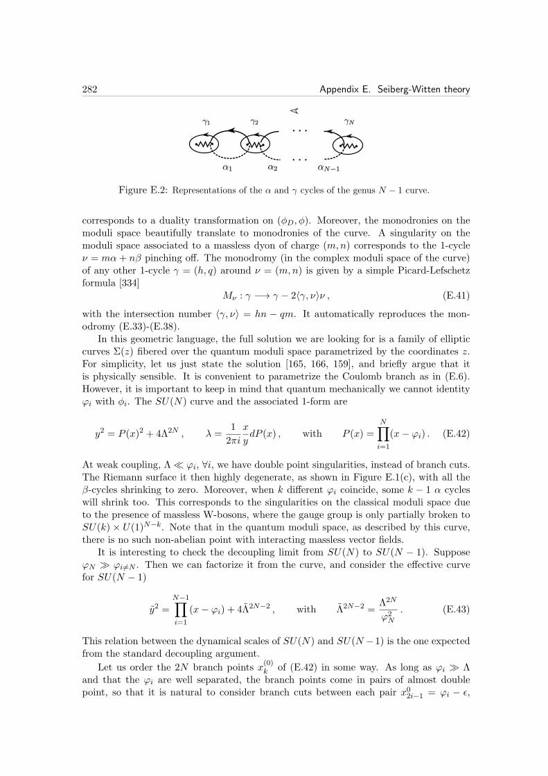
282 Appendix E. Seiberg-Witten theory
Figure E.2: Representations of the α and γ cycles of the genus N − 1 curve.
corresponds to a duality transformation on (φD, φ). Moreover, the monodronies on themoduli space beautifully translate to monodronies of the curve. A singularity on themoduli space associated to a massless dyon of charge (m,n) corresponds to the 1-cycleν = mα+ nβ pinching off. The monodromy (in the complex moduli space of the curve)of any other 1-cycle γ = (h, q) around ν = (m,n) is given by a simple Picard-Lefschetzformula [334]
Mν : γ −→ γ − 2〈γ, ν〉ν , (E.41)
with the intersection number 〈γ, ν〉 = hn − qm. It automatically reproduces the mon-odromy (E.33)-(E.38).
In this geometric language, the full solution we are looking for is a family of ellipticcurves Σ(z) fibered over the quantum moduli space parametrized by the coordinates z.For simplicity, let us just state the solution [165, 166, 159], and briefly argue that itis physically sensible. It is convenient to parametrize the Coulomb branch as in (E.6).However, it is important to keep in mind that quantum mechanically we cannot identityϕi with φi. The SU(N) curve and the associated 1-form are
y2 = P (x)2 + 4Λ2N , λ =1
2πi
x
ydP (x) , with P (x) =
N∏
i=1
(x− ϕi) . (E.42)
At weak coupling, Λ≪ ϕi, ∀i, we have double point singularities, instead of branch cuts.The Riemann surface it then highly degenerate, as shown in Figure E.1(c), with all theβ-cycles shrinking to zero. Moreover, when k different ϕi coincide, some k − 1 α cycleswill shrink too. This corresponds to the singularities on the classical moduli space dueto the presence of massless W-bosons, where the gauge group is only partially broken toSU(k) × U(1)N−k. Note that in the quantum moduli space, as described by this curve,there is no such non-abelian point with interacting massless vector fields.
It is interesting to check the decoupling limit from SU(N) to SU(N − 1). SupposeϕN ≫ ϕi 6=N . Then we can factorize it from the curve, and consider the effective curvefor SU(N − 1)
y2 =N−1∏
i=1
(x− ϕi) + 4Λ2N−2 , with Λ2N−2 =Λ2N
ϕ2N
. (E.43)
This relation between the dynamical scales of SU(N) and SU(N −1) is the one expectedfrom the standard decoupling argument.
Let us order the 2N branch points x(0)k of (E.42) in some way. As long as ϕi ≫ Λ
and that the ϕi are well separated, the branch points come in pairs of almost doublepoint, so that it is natural to consider branch cuts between each pair x02i−1 = ϕi − ǫ,
E.5. SW curves for N = 2 SQCD with Nf flavors 283
x02i = ϕi + ǫ; this semi-classical understanding was used to draw Figure E.1(b). Let uscall γi the 1-cycle which circles around the almost double point at x = ϕi (note that∑N
i=1 γi = 0). One can check that, in the classical limit,
φi =
∮
γi
λ =1
2πi
∮
γi
xP ′(x)
Pdx+ o(Λ) = ϕi + o(Λ) . (E.44)
Let us call αa the 1-cycle which goes from x02a+1 to x02a on the upper sheet, and back onthe lower sheet, for a = 1, · · · , N − 1. These cycles are represented in Figure E.2. Let usalso define the N − 1 independent cycles
βa =∑
i≤a
γi . (E.45)
These are the cycles appearing in (E.40). One can check that 〈αa, βb〉 = δab.
E.5 SW curves for N = 2 SQCD with Nf flavors
Consider N = 2 SQCD, namely the SU(N) theory coupled to Nf hypermultiplets (fla-vors). In N = 1 notation, the hypermultiplets (Q, Q†) are coupled to the adjoint chiralfield Φ through the superpotential
W =√2QjΦQ
j +∑
j
mjQjQj , (E.46)
with j = 1, · · · , Nf . We allow for arbitrary N = 2 preserving masses for the hypermulti-plets. The various branches of the moduli space of this theory were studied in detail in[155]. We can distinguish between the Higgs branches and the Coulomb branch. On theformer the hypermultiplets get a VEV and the gauge group is fully broken. The classicalmetric on the Higgs branch is not renormalized in a N = 2 theory. On the other handthe Coulomb branch looks classicaly similar to the one of the pure SU(N) SYM theory,since a generic non-zero VEV for Φ gives a mass to all the hypermultiplets. The crucialnew phenomenon can appear at places where the Coulomb branch meets a Higgs branch.In particular, the locus of interesection can change non-perturbatively, giving rise to adual interpretation of the low energy physics. We review the relevant such facts when weneed then in Chapter 6.
In the case of non-zero masses mj , the non-perturbative central charge formula be-comes [80]
Z = haφaD + qaφa + njmj , (E.47)
where nj is the charge under the U(1) flavor symmetry acting on the hypermultiplet ofmass mj . The duality group leaving Z invariant is a larger group Sl(2, 2N − 2,Z)⋉Z
Nf ,so that the fields (aD, a) characterizing the Coulomb branch are a section of a morecomplicated bundle. We are mostly interested in the case mj = 0 anyway. The Seiberg-Witten curve for N = 2 SQCD with Nf < 2N is [80, 169, 171]
y2 = P (x)2 + 4Λ2N−Nf
Nf∏
j=1
(x+mj) , , with P (x) =N∏
i=1
(x− ϕi) . (E.48)

284 Appendix E. Seiberg-Witten theory
For Nf > 2N the theory is IR free, and the description in term of the curve (E.48)breaks down above some scale of order Λ. The case Nf = 2N is special, because theexact beta function identically vanishes and the theory is conformal. The determinationof the Seiberg-Witten curve in that case [80, 169] is a rather subtle issue, related to thepossibility of having a S-duality invariant theory (similarly to N = 4 SYM). We remarkthat the SW curve for the Nf = 2N elliptic quiver of Chapter 6 might be better motivatedthan the similar curve in the usual Nf = 2Nc theory, due to the clearer string theoryembedding of the elliptic quiver.
E.6 SW curves from M-theory
A suprisingly simple relationship between the Seiberg-Witten theory approach to N =2 gauge theories on the one hand and string theory/M-theory on the other hand wasuncovered by Witten [157] using the type IIA/M-theory duality. Consider two paralleltype IIA NS5-branes separated by a distance L = ∆x6 in the x6 direction, and a bunchof N D4-branes stretching between them:
0 1 2 3 4 5 6 7 8 9
NS5 NS5’ D4
(E.49)
This setup brane-engineers N = 2 U(N) SYM. The boundary condition for the D4-braneending on the NS5-brane sets to zero the A6 component of the gauge field 5, as well asthe scalar fields corresponding to x7, x8, x9. At energies smaller than 1/L, the low energytheory is four dimensional N = 2 SYM. The complex scalar in the N = 2 multipletcorresponds to motion of the D4-branes along the NS5-branes, in the v = x4 + ix5
direction. The gauge coupling of the low energy theory is
8π2
g2=
∆x6√α′gs
. (E.50)
The perturbative beta function for g can be accounted for by the bending of the NS5-branes due to the D4-branes tension: the D4-brane sources the field responsible for the x6
profile of each NS5-brane. The log v solution of the resulting Laplace equation reproducesthe perturbative running of g [157], because the radius |v| can be related to the VEV ofa (probe) eigenvalue of the adjoint field, which is in turn related to the RG scale in aN = 2 theory.
The crucial observation is that the non-perturbative corrections to the low energytheory can be captured by uplifting the IIA setup to M-theory. This means that wetake R10 =
√α′gs large. We want to do that while keeping the gauge coupling fixed,
so we rescale the distance L to be large too. Remark that this limit R10, L → ∞ seemsopposite to the field theory limit. However, what makes it useful is that we have N = 2supersymmetry, in which case the LEEA only depends on holomorphic quantities. InM-theory, the IIA fivebranes and D4-branes all lift to a single smooth M5-brane. The
5It follows by T-duality from the type IIB setup of [54].
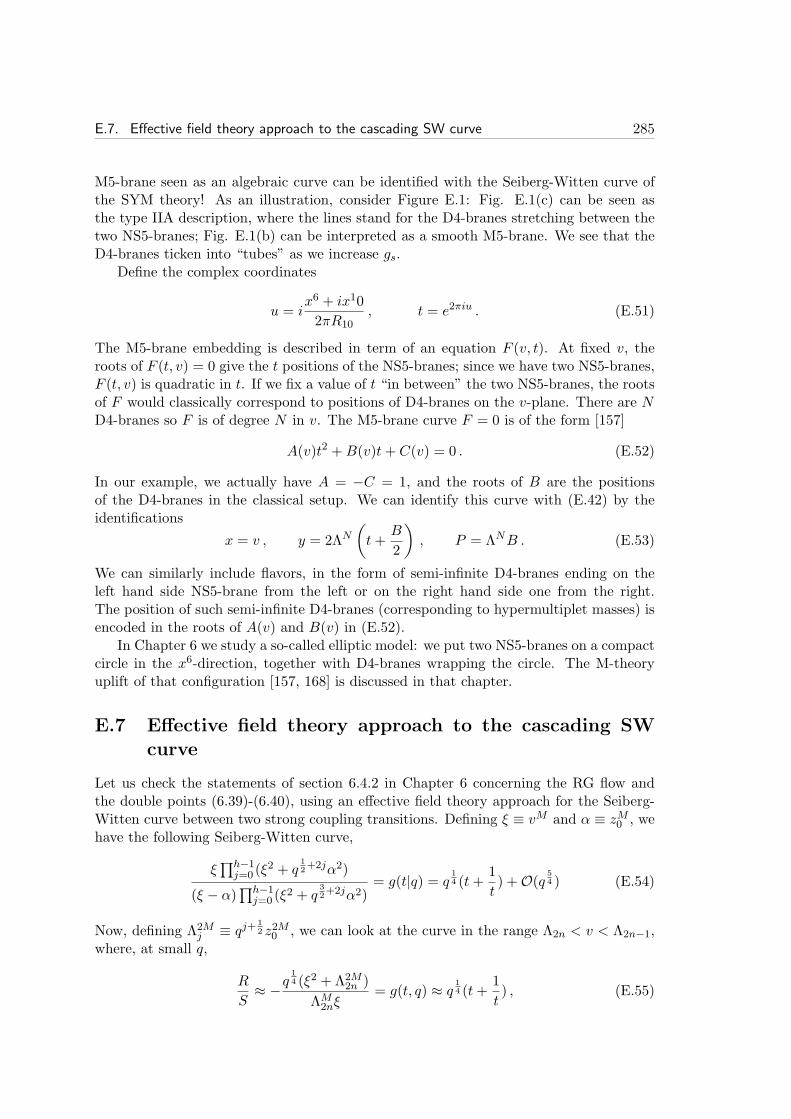
E.7. Effective field theory approach to the cascading SW curve 285
M5-brane seen as an algebraic curve can be identified with the Seiberg-Witten curve ofthe SYM theory! As an illustration, consider Figure E.1: Fig. E.1(c) can be seen asthe type IIA description, where the lines stand for the D4-branes stretching between thetwo NS5-branes; Fig. E.1(b) can be interpreted as a smooth M5-brane. We see that theD4-branes ticken into “tubes” as we increase gs.
Define the complex coordinates
u = ix6 + ix10
2πR10, t = e2πiu . (E.51)
The M5-brane embedding is described in term of an equation F (v, t). At fixed v, theroots of F (t, v) = 0 give the t positions of the NS5-branes; since we have two NS5-branes,F (t, v) is quadratic in t. If we fix a value of t “in between” the two NS5-branes, the rootsof F would classically correspond to positions of D4-branes on the v-plane. There are ND4-branes so F is of degree N in v. The M5-brane curve F = 0 is of the form [157]
A(v)t2 +B(v)t+ C(v) = 0 . (E.52)
In our example, we actually have A = −C = 1, and the roots of B are the positionsof the D4-branes in the classical setup. We can identify this curve with (E.42) by theidentifications
x = v , y = 2ΛN(
t+B
2
)
, P = ΛNB . (E.53)
We can similarly include flavors, in the form of semi-infinite D4-branes ending on theleft hand side NS5-brane from the left or on the right hand side one from the right.The position of such semi-infinite D4-branes (corresponding to hypermultiplet masses) isencoded in the roots of A(v) and B(v) in (E.52).
In Chapter 6 we study a so-called elliptic model: we put two NS5-branes on a compactcircle in the x6-direction, together with D4-branes wrapping the circle. The M-theoryuplift of that configuration [157, 168] is discussed in that chapter.
E.7 Effective field theory approach to the cascading SW
curve
Let us check the statements of section 6.4.2 in Chapter 6 concerning the RG flow andthe double points (6.39)-(6.40), using an effective field theory approach for the Seiberg-Witten curve between two strong coupling transitions. Defining ξ ≡ vM and α ≡ zM0 , wehave the following Seiberg-Witten curve,
ξ∏h−1j=0 (ξ
2 + q12+2jα2)
(ξ − α)∏h−1j=0 (ξ
2 + q32+2jα2)
= g(t|q) = q14 (t+
1
t) +O(q 5
4 ) (E.54)
Now, defining Λ2Mj ≡ qj+
12 z2M0 , we can look at the curve in the range Λ2n < v < Λ2n−1,
where, at small q,
R
S≈ −q
14 (ξ2 + Λ2M
2n )
ΛM2nξ= g(t, q) ≈ q 1
4 (t+1
t) , (E.55)

286 Appendix E. Seiberg-Witten theory
which givesξΛM2nt
2 + (ξ2 + Λ2M2n )t+ ξΛM2n = 0, (E.56)
This is a SW curve for a SU(2M) gauge group with 2M massless flavors [157], at thebaryonic root (hence it has exact double points). Extracting the roots for t (and neglectingΛn/v because of large M), one finds
u1 = −u2 = −M
2πilog
(v
Λ2ne−
2πik2M
)
= − M
2πilog
v
Λ2n+
1
2k, (E.57)
where k = 0, 1. We see that at v = Λ2n, u1 = u2 = 0, 12 (that is, the two NS5’s intersect atx6 = 0, but in fact the corresponding M5 brane also self-intersects at two distinct pointson the torus). Since τ1 = u2 − u1 = τ − τ2, we have reproduced the correct perturbativerunning of the gauge couplings. Also notice that this effective field theory for the firstnode is valid only up to v = Λ2n−1, where according to (E.57) u1 = u2 = τ
2 ,τ2 + 1
2 (thatis when the coupling of the second gauge group hits a Landau pole).
One can perform the same analysis for the second gauge group, i.e. for the doublepoints at u = τ
2 ,τ2 + 1
2 , obtaining (6.40).

Appendix F
The conifold and a Z2 orbifoldthereof
F.1 Generalities on the conifold geometry
The singular conifold C0 can be defined as an affine variety in C4 ∼= z1, z2, z3, z4,
z1z2 − z3z4 = 0 . (F.1)
By a linear change of coordinates, this can also be written as: w21 + w2
2 + w23 + w2
4 = 0.The conifold is a CY cone, whose base is a Sasaki-Einstein manifold called T 1,1 [104].The latter is described algebraically by the intersection of the cone with a unit sphere inC4:∑4
i=1 |wi|2 = 1. In terms of real coordinates, wi = xi + iyi, one gets ~x · ~x = 1/2,~y · ~y = 1/2, ~x · ~y = 0, which can be seen as an S2 fibration over S3. However such afibration is trivial1, so that topologically T 1,1 ∼= S2×S3. The following coordinate systemon the cone will be useful2
z1 = r3/2 ei2(ψ+φ1+φ2) sin
θ12sin
θ22, (F.2)
z2 = r3/2 ei2(ψ−φ1−φ2) cos
θ12cos
θ22, (F.3)
z3 = r3/2 ei2(ψ−φ1+φ2) cos
θ12sin
θ22, (F.4)
z4 = r3/2 ei2(ψ+φ1−φ2) sin
θ12cos
θ22. (F.5)
Here, 0 ≤ ψ ≤ 4π , 0 ≤ φi ≤ 2π , 0 ≤ θi ≤ π, and we have the following angularperiodicities
ψφ1φ2
≃
ψ + 4πφ1φ2
≃
ψ + 2πφ1 + 2πφ2
≃
ψ + 2πφ1
φ2 + 2π
. (F.6)
1We can cover S3 with two patches, intersecting at the equator. The bundle is constructed by specifyinga transition function on this equator (itself an S2), which is a map from S2 to SO(3), the structure groupof the fiber. Such maps are always trivial (π2(SO(3)) = 0), so the bundle is trivial.
2Remark that we differ from the conventions of [118] by a flip in the orientation of the angles φi.
287

288 Appendix F. The conifold and a Z2 orbifold thereof
In these coordinates, the Calabi-Yau metric reads: ds2C0= dr2 + r2 ds2T 1,1 , with the
Sasaki-Einstein metric of T 1,1
ds2T 1,1 =∑
i=1,2
1
6
(dθ2i + sin2 θi dφ
2i
)+
1
9
(dψ −
∑
i=1,1
cos θi dφi)2. (F.7)
It describes a circle bundle, where the circle ψ is fibered over S2 × S2. In terms of thenatural vielbein for the two 2-spheres, ui = dθi, vi = sin θi dφi (i = 1, 2), it is useful todefine rotated vielbein for the 2-spheres [335]
(σ1σ2
)
=
(cos ψ2 − sin ψ
2
sin ψ2 cos ψ2
)(u1v1
) (Σ1
Σ2
)
=
(cos ψ2 − sin ψ
2
sin ψ2 cos ψ2
)(u2v2
)
. (F.8)
Let us also define ζ = dψ −∑i=1,2 cos θi dφi. For the singular conifold, we will use thefollowing ordered vielbein
er = dr , eψ =r
3ζ , e1 =
r√6σ1 , e
2 =r√6σ2 , e
3 =r√6Σ1 , e
4 =r√6Σ2
. (F.9)
The metric of the conifold then reads ds2C0=∑6
n=1 (en)2, and the volume form is
dvolC0 = er∧eψ∧e1∧e2∧e3∧e4 = 1
108r5 dr∧dψ∧dθ1∧sin θ1 dφ1∧dθ2∧sin θ2 dφ2 . (F.10)
A complex vielbein can be defined as
E1 = e1 + ie2 , E2 = e3 + ie4 , E3 = er + ieψ
. (F.11)
In terms of this complex structure, the Kahler form is
J ≡ i
2
(
E1 ∧ E1 + E2 ∧ E2 + E3 ∧ E3)
= d
(r2
6ζ
)
, (F.12)
which is (1, 1), closed and satisfies J ∧ J ∧ J = 6 dvolC0 . It is exact, since we are at thezero resolution point in Kahler moduli space where the cohomology class of J is trivial.The holomorphic top form is
Ω(3,0) ≡ E1 ∧ E2 ∧ E3 = −4
9
dz1 ∧ dz2 ∧ dz3z3
. (F.13)
Let us now review 2- and 3-(co)cycles for the conifold. We have the closed (1,1)-form
ωCF2 ≡ 3i
2r2
(
E1 ∧ E1 − E2 ∧ E2)
=1
2(σ1 ∧ σ2 − Σ1 ∧ Σ2) =
=1
2(sin θ1 dθ1 ∧ dφ1 − sin θ2 dθ2 ∧ dφ2) .
(F.14)
The 2-cycle in T 1,1 is topologically a 2-sphere CCF . It can be represented by
CCF : θ1 = θ2 ≡ θ , φ1 = 2π − φ2 ≡ φ , ψ = 0 , φ ∈ [0, 2π) , θ ∈ (0, π) .(F.15)

F.2. The orbifolded conifold geometry 289
It turns out that∫
CCFωCF2 = 4π. In addition, one usually defines the real closed 3-form
ωCF3 ≡ ζ ∧ ωCF2 , (F.16)
which is the real part of the imaginary-self-dual (ISD) primitive (2,1)-form
ω(2,1) ≡ 9
2r3E3 ∧
(
E1 ∧ E1 − E2 ∧ E2)
=
(
ζ − 3idr
r
)
∧ ωCF2 , (F.17)
defined on the whole conifold. Imaginary self-duality means that ∗6 ω(2,1) = i ω(2,1). The3-cycle in T 1,1 has the topology of a 3-sphere. We call it ACF . It can be represented by
ACF : θ2 = φ2 = 0 . (F.18)
Its orientation is such that∫
ACFωCF3 = 8π2.
F.2 The orbifolded conifold geometry
In this appendix, we derive the results presented in section 7.2 concerning the relationbetween the ranks in the quiver, the cycles wrapped by the different fractional branes, andthe fluxes present in the supergravity solution. In order to do this, we need first to discussin detail the compact 2-cycles of the geometry, on which the branes can wrap. Then wediscuss the compact 3-cycles of the geometry, which support the RR fluxes sourced bythe branes, and their intersections with the 2-cycles (in the base of the singular cone).This will allow us to write the 3-form fluxes directly in terms of the ranks of the gaugegroups in the quiver.
The CY singularity on which our gauge theory is engineered is a non-chiral Z2 orbifoldof the conifold (F.1), obtained considering the following action on the coordinates zi inC4
Θ : (z1, z2, z3, z4) → (z1, z2,−z3,−z4) . (F.19)
The orbifold geometry is still an algebraic variety. To describe it one can introduce acomplete set of invariants: x ≡ z23 , y ≡ z24 and t ≡ z3z4, which satisfy the constraintxy = t2. The conifold equation is rewritten as t = z1z2 so that t can be eliminated andwe are left with
f = (z1z2)2 − xy = 0 . (F.20)
The singular locus f = df = 0 consists of two complex lines that meet at the tip of thegeometry z1 = z2 = x = y = 0, and corresponds to the fixed point locus of the orbifoldaction Θ.
One can use real coordinates as well, those already defined in appendix F.1. Theorbifold action (F.19), which is an identification in the covering space, where we willwork, reads
Θ : (φ1, φ2) → (φ1 − π, φ2 + π) . (F.21)
The two complex lines, that we call the p and q line respectively, are defined, in complexand real coordinates, as
p = z1 = x = y = 0, ∀z2 = θ1 = θ2 = 0, ∀r, ψ′ (F.22)
q = z2 = x = y = 0, ∀z1 = θ1 = θ2 = π, ∀r, ψ′′ , (F.23)

290 Appendix F. The conifold and a Z2 orbifold thereof
where ψ′ = ψ − φ1 − φ2 and ψ′′ = ψ + φ1 + φ2 are (well defined) angular coordinatesalong the singularity lines. In a neighborhood of the singular lines (and outside the tip)the geometry looks locally like the A1-singularity C×C
2/Z2. The fixed point curve p sitsat the north poles of both S2’s while the curve q sits at the south poles.
2-cycles and resolutions
From the above analysis it follows that the singular geometry has three vanishing 2-cycles.Two of these three cycles arise due to the orbifold action; such exceptional 2-cycles arelocated all along the C
2/Z2 singular lines p and q (F.22), and we call them C2 and C4,respectively. Locally, one could resolve the space into an ALE space fibered over C∗. Thethird relevant 2-cycle descends from the 2-cycle of the double covering conifold geometry,whose base T 1,1 is topologically S2 × S3.
Our goal in what follows is to pinpoint the precise map between vanishing 2-cycles,wrapped D5-branes, 3-form RR fluxes and quiver rank assignments. To this end, itwill prove useful to take advantage of our CY cone being a toric variety3, since in thiscase one can use standard techniques to understand the structure of 2-cycles and theirintersections. Let us sketch how this comes about.
A toric variety can be described as the moduli space of an associated supersymmetricgauged linear σ-model (GLSM). Consider n chiral superfields ti, i = 1 . . . n charged undera product of abelian gauge groups U(1)s, with charges Q i
a , a = 1 . . . s. In the absence ofa superpotential, the potential for the scalar components is
V (ti) =s∑
a=1
( n∑
i=1
Q ia |ti|2 − ξa
)2. (F.24)
where ξa are Fayet-Iliopoulos parameters (FI). The moduli space of vacuaM is given bythe D-flatness equations modulo U(1)s gauge transformations
M =
ti ∈ Cn∣∣∣
n∑
i=1
Q ia |ti|2 = ξa ∀a = 1, . . . , s
/
U(1)s , (F.25)
where U(1)s acts as ti → eiQia φati. When the FI’s are such that dimM = n − s, M is
the desired toric variety (and n − s = r is just the number of isometry abelian factors).Putting the FI’s to zero the variety, if admissible, is scale invariant: this corresponds toa cone. As the FI’s change, the Kahler moduli ofM also change and one gets resolutionsor blow-ups. Generically, different regions in the parameter space of the FI parameterscorrespond to different resolutions, delimited by flop transition curves.
In our case the GLSM has six fields ti whose charges Q ia are reported in the table
belowt1 t2 t3 t4 t5 t60 0 1 −2 1 0 ξ21 −1 0 1 −1 0 ξβ−2 1 0 0 0 1 ξ4
(F.26)
3A toric manifold is a manifold of complex dimension r which admits an isometry group (at least asbig as) U(1)r. A toric CY threefold is then a CY threefold whose isometry group is at least U(1)3. For arecent introduction, see e.g. [288].

F.2. The orbifolded conifold geometry 291
Figure F.1: The toric diagram and the dual (p, q)-web. The specific toric diagram triangulationis the one related to having all ξa > 0 in the associated GLSM.
We can parameterize the toric variety with the gauge invariants
t3t4t5 = z1 t1t2t6 = z2 t1t22t
23t4 = x t1t4t
25t
26 = y (F.27)
which, consistently, satisfy the defining equation (F.20). We can also give a parametriza-tion for the so-called toric divisors, which are the four-dimensional hypersurfaces in thetoric CY defined by Di = ti = 0. We recognize D4 = z1 = x = y = 0 as the p lineand D1 = z2 = x = y = 0 as the q-line.
The toric diagram and the related (p, q)-web corresponding to choosing all ξa > 0(which amounts to a given triangulation of the toric diagram) are depicted in FigureF.1. For the particular resolution corresponding to ξ2, ξβ, ξ4 > 0 the three holomorphic2-cycles can be directly read from the (p, q)-web. They can be explicitly constructed asintersections of toric divisors
C2 = D2 ·D4 Cβ = D2 ·D5 C4 = D1 ·D5 . (F.28)
This can be explicitly checked using D-term equations, which for the intersections ofinterest are
D2D4 : |t3|2 + |t5|2 = ξ2 |t6|2 = 2|t1|2 + ξ4 |t1|2 = |t5|2 + ξβ (F.29)
D2D5 : |t4|2 + |t1|2 = ξβ |t3|2 = 2|t4|2 + ξ2 |t6|2 = 2|t1|2 + ξ4 (F.30)
D1D5 : |t2|2 + |t6|2 = ξ4 |t3|2 = 2|t4|2 + ξ2 |t4|2 = |t2|2 + ξβ . (F.31)
As one can see, each Ci topologically is a CP1 (parameterized by the first two variablesin each row) of volume ξi.
Let us consider also another basis of 2-cycles, which arises in a different resolutionof the singular conical geometry (corresponding to a different triangulation of the toricdiagram). Consider the region in the space of FI parameters where ξβ < 0 with ξ2+ξβ > 0and ξ4 + ξβ > 0. We can introduce
ξ1 = ξ4 + ξβ > 0 ξ3 = ξ2 + ξβ > 0 ξα = −ξβ > 0 . (F.32)
This new resolution can be obtained from the one in Figure F.1 with a flop transitionon Cβ ↔ Cα. The toric diagram triangulation and the corresponding dual (p, q)-web forthe new geometry are sketched in Figure F.2. In order to have a nice presentation of the

292 Appendix F. The conifold and a Z2 orbifold thereof
Figure F.2: The toric diagram and the dual (p, q)-web in the region of the FI parameter spacewhere ξβ < 0.
GLSM charges in terms of the new positive FI’s, we can linearly re-shuffle Table (F.26)getting
t1 t2 t3 t4 t5 t6−1 0 0 1 −1 1 ξ1−1 1 0 −1 1 0 ξα1 −1 1 −1 0 0 ξ3
(F.33)
Repeating the same analysis as before one finds the holomorphic4 2-cycles in this newresolution in terms of toric divisors
C3 = D2 ·D4 Cα = D1 ·D4 C1 = D1 ·D5 . (F.34)
Again the FI parameters are the positive volumes of the corresponding 2-cycles Ci. Fromthe relations among FI parameters we read the relations
C1 = C4 + Cβ C3 = C2 + Cβ , (F.35)
which can be thought of as relations in homology between vanishing cycles.
A comment is in order at this point. In this non-chiral case, vanishing 2-cycles arein one-to-one correspondence with possible fractional branes. All the divisors are noncompact 4-cycles. This implies that all dual 2-cycles support non-anomalous fractionalbranes. This does not hold in general, as only 2-cycles dual to non-compact 4-cycles giveanomaly-free fractional branes, their number being equal to the number of 3-cycles in thereal base of the CY cone (which in turn corresponds to the number of baryonic charges).This is the geometric counterpart of the dual gauge theory being non-chiral. Conversely,chiral theories are related to CY cones where there are compact 4-cycles around. Thelatter put constraints on the allowed fractional D3-branes configurations, because of theRR tadpole cancellation condition.
Once we wrap a D5-brane on a 2-cycle, it will thus source a 3-form RR flux. We turnto consider the compact 3-cycles of the geometry which can support this flux, and theirdual non-compact 3-cycles.
4Notice that generically if an homology class C has a holomorphic representative, −C does not becausethe representative becomes antiholomorphic and one should look for a different one. In particular, indifferent resolutions the role of homology classes with a holomorphic representative is exchanged.
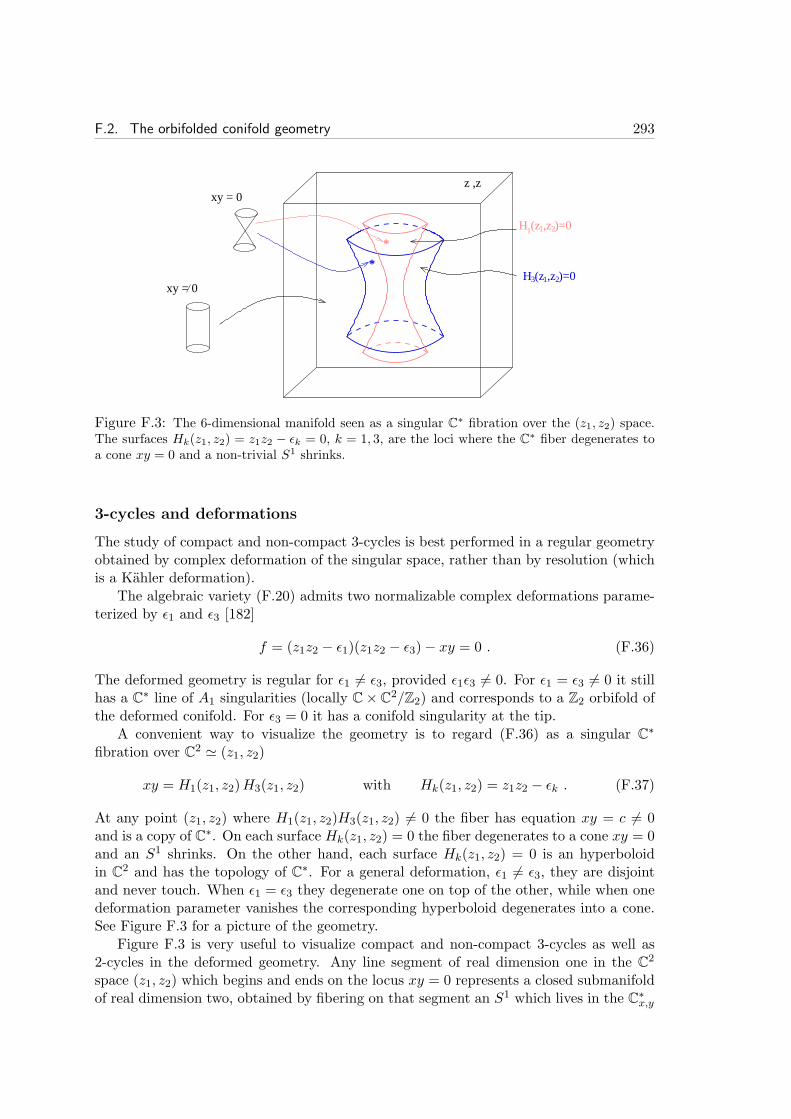
F.2. The orbifolded conifold geometry 293
z ,z
1H (z ,z )=0
xy = 0
xy = 0
*
*1 23H (z ,z )=0
1 2
Figure F.3: The 6-dimensional manifold seen as a singular C∗ fibration over the (z1, z2) space.
The surfaces Hk(z1, z2) = z1z2 − ǫk = 0, k = 1, 3, are the loci where the C∗ fiber degenerates to
a cone xy = 0 and a non-trivial S1 shrinks.
3-cycles and deformations
The study of compact and non-compact 3-cycles is best performed in a regular geometryobtained by complex deformation of the singular space, rather than by resolution (whichis a Kahler deformation).
The algebraic variety (F.20) admits two normalizable complex deformations parame-terized by ǫ1 and ǫ3 [182]
f = (z1z2 − ǫ1)(z1z2 − ǫ3)− xy = 0 . (F.36)
The deformed geometry is regular for ǫ1 6= ǫ3, provided ǫ1ǫ3 6= 0. For ǫ1 = ǫ3 6= 0 it stillhas a C
∗ line of A1 singularities (locally C× C2/Z2) and corresponds to a Z2 orbifold of
the deformed conifold. For ǫ3 = 0 it has a conifold singularity at the tip.A convenient way to visualize the geometry is to regard (F.36) as a singular C
∗
fibration over C2 ≃ (z1, z2)
xy = H1(z1, z2)H3(z1, z2) with Hk(z1, z2) = z1z2 − ǫk . (F.37)
At any point (z1, z2) where H1(z1, z2)H3(z1, z2) 6= 0 the fiber has equation xy = c 6= 0and is a copy of C∗. On each surface Hk(z1, z2) = 0 the fiber degenerates to a cone xy = 0and an S1 shrinks. On the other hand, each surface Hk(z1, z2) = 0 is an hyperboloidin C
2 and has the topology of C∗. For a general deformation, ǫ1 6= ǫ3, they are disjointand never touch. When ǫ1 = ǫ3 they degenerate one on top of the other, while when onedeformation parameter vanishes the corresponding hyperboloid degenerates into a cone.See Figure F.3 for a picture of the geometry.
Figure F.3 is very useful to visualize compact and non-compact 3-cycles as well as2-cycles in the deformed geometry. Any line segment of real dimension one in the C
2
space (z1, z2) which begins and ends on the locus xy = 0 represents a closed submanifoldof real dimension two, obtained by fibering on that segment an S1 which lives in the C∗
x,y
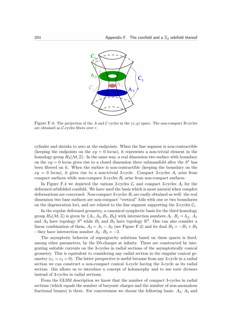
294 Appendix F. The conifold and a Z2 orbifold thereof
A 3
A 1
A 2 C
C
C
2
3
1
Figure F.4: The projection of the A and C cycles in the (x, y) space. The non-compact B-cyclesare obtained as C-cycles fibers over r.
cylinder and shrinks to zero at the endpoints. When the line segment is non-contractible(keeping the endpoints on the xy = 0 locus), it represents a non-trivial element in thehomology group H2(M,Z). In the same way, a real dimension two surface with boundaryon the xy = 0 locus gives rise to a closed dimension three submanifold after the S1 hasbeen fibered on it. When the surface is non-contractible (keeping the boundary on thexy = 0 locus), it gives rise to a non-trivial 3-cycle. Compact 3-cycles Ai arise fromcompact surfaces while non-compact 3-cycles Bi arise from non-compact surfaces.
In Figure F.4 we depicted the various 2-cycles Ci and compact 3-cycles Ai for thedeformed orbifolded conifold. We have used the basis which is most natural when complexdeformations are concerned. Non-compact 3-cycles Bi are easily obtained as well: the realdimension two base surfaces are non-compact “vertical” foils with one or two boundarieson the degeneration loci, and are related to the line segment supporting the 2-cycles Ci.
In the regular deformed geometry, a canonical symplectic basis for the third homologygroup H3(M,Z) is given by A1, A3, B1, B3 with intersection numbers Ai ·Bj = δij . A1
and A3 have topology S3 while B1 and B3 have topology R3. One can also consider a
linear combination of them, A2 = A1 −A3 (see Figure F.4) and its dual B2 = −B1 +B3
: they have intersection number A2 ·B2 = −2.The asymptotic behavior of supergravity solutions based on these spaces is fixed,
among other parameters, by the D5-charges at infinity. These are constructed by inte-grating suitable currents on the 3-cycles in radial sections of the asymptotically conicalgeometry. This is equivalent to considering any radial section in the singular conical ge-ometry (ǫ1 = ǫ3 = 0). The latter perspective is useful because from any 3-cycle in a radialsection we can construct a non-compact conical 4-cycle having the 3-cycle as its radialsection: this allows us to introduce a concept of holomorphy and to use toric divisorsinstead of 3-cycles in radial sections.
From the GLSM description we know that the number of compact 3-cycles in radialsections (which equals the number of baryonic charges and the number of non-anomalousfractional branes) is three. For concreteness we choose the following basis: A2, A4 and
F.2. The orbifolded conifold geometry 295
ACF . A2 is the radial section of the toric divisor D4, and corresponds to the productof the exceptional 2-cycle C2 along the p-line (which is ∼= C
∗) with S1 in the latter; inthe same way, A4 is the radial section of the toric divisor D1, and is the product of theexceptional C4 along the q-line times S1. ACF is the compact 3-cycle of the covering spaceconifold5: under the orbifold action it has an image, and no fixed points. In particular, therepresentative 3-cycle at θ2 = π/2 and φ2 = 0 is mapped to the divisor x = z21 , y = z22which has the GLSM description t1t
22 = t4t
25. Comparing the charges we find that ACF
corresponds to the toric divisor D1+2D2 = D4+2D5. Summarizing, our basis of 3-cyclesand the corresponding toric divisors are
A2 ≃ D4 A4 ≃ D1 ACF ≃ D1 + 2D2 = D4 + 2D5 . (F.38)
Notice that in the deformed geometry A2 = −A4 in homology. Nevertheless they cangive rise to different charges when explicit sources are present in the geometry and thisis in fact the case of N = 2 branes which do not undergo complete geometric transition.
In order to compute the 3-form fluxes generated by D5-branes wrapped on 2-cycles,we will need the intersection matrix between divisors and 2-cycles. In our basis we find
A2 ≃ D4 A4 ≃ D1 ACFC2 −2 0 0C4 0 −2 0Cβ 1 1 −1
(F.39)
This table is computed from the charges in Table (F.26): in the GLSM constructioneach gauge field gives rise to an element Ca of the homology group H2(M,Z), and theintersection between it and a toric divisor Di is the charge Q i
a .
The fractional branes/ranks correspondence
We have now all the ingredients to finally figure out the precise correspondence betweenfractional branes (that is wrapped D5-branes) and quiver rank assignments.
Consider a D5-brane wrapped on a 2-cycle Ci of our CY3. The Bianchi identity forF3 is violated by the source
dF3 = −2κ2τ5Ω4 , (F.40)
where Ω4 is a 4-form with δ-function support on the D5 world-volume. We are interestedin the flux generated on a 3-cycle Aj in the radial section. First we have to resolve thegeometry, switching on the FI parameters of the associated GLSM. This does not changethe holomorphic data nor the quantized charges. Then we identify a non-compact divisorDj which has Aj as radial section. Being the geometry smooth, Aj turns out to be theboundary of Dj
∫
Aj
F3 = −∫
Dj
dF3 = 2κ2τ5
∫
Dj
Ω4 = 2κ2τ5 (Dj , Ci) , (F.41)
where (Dj , Ci) is the intersection number as in Table (F.39), and we fixed the orientationambiguity requiring consistency with known cases, such as the conifold and the Z2 orbifold
5Actually ACF = A1 +A3.

296 Appendix F. The conifold and a Z2 orbifold thereof
of R6. If there is a holomorphic representative for Ci, we can then directly compute theintersection from the GLSM data.
The last thing to determine are the quiver rank assignments corresponding to eachfractional brane. A D5-brane wrapped on the exceptional 2-cycles C2 and C4 along theC2/Z2 lines p and q gives rise to an N = 2 fractional brane, and we conventionally choose
the rank assignments to be, respectively, (0, 1, 1, 0) and (1, 1, 0, 0). The rank assignmentfor a D5-brane wrapped on Cβ can be defined by observing that the combination CCF =2Cβ + C2 + C4 does not couple to twisted fields and gives rise to the orbifold of theKlebanov-Tseytlin theory [127], see Table (F.39). This implies that the correspondinggauge theory is the orbifold of the KT theory. We can say that the ranks for one D5 onCβ are (a, b, c, d). Requiring that 2Cβ + C2 + C4 is in the class (N + 1, N,N + 1, N) or(N,N + 1, N,N + 1), which do correspond to the orbifold of the KT theory, singles outtwo possibilities for Cβ : either (1, 0, 1, 1) or (0, 0, 0, 1). To select the correct option weshould consider the induced D3-charge on the fractional D3 probe.
The induced D3-charge is proportional to the integral of B2 (or more generally ofF = B2 + 2πα′F2) on the corresponding 2-cycle C:
Q3 = τ5
∫
CF = τ3
1
4π2α′
∫
C
(B2 + 2πα′F
). (F.42)
The actual value depends on the background value of B2. This is arbitrary at this level(and it is related to the UV cut-off values of the gauge couplings in the dual gauge the-ory). We only require these background values to be positive (so as to describe mutuallyBPS objects) and less than one (in order to describe non-composite, that is elementary,objects). Along the p and q lines the physics is locally C
2/Z2, thus we can naturallyset [39]:
∫
C2B2 =
∫
C4B2 = (4π2α′)/2. If we consider the KT theory and set also [127]
∫
CCFB2 = (4π2α′)/2, then using the previous relation CCF = 2Cβ + C2 + C4, we get
∫
CβB2 = −(4π2α′)/4.
This implies that while the N = 2 branes have positive D3-charge, a D5-branewrapped on Cβ has negative D3-brane charge and it is not mutually BPS. Putting oneunit of worldvolume flux on the wrapped D5 we get positive D3-charge: 3/4. The totalD3-charge for CCF = 2Cβ +C2+C4 (with two units of flux on Cβ) is 5/2. This is exactlythe D3-charge of the configuration (3, 2, 3, 2), which implies that one D5-brane wrappedon Cβ with one unit of worldvolume flux gives rise to the theory (1, 0, 1, 1). A similaranalysis shows that a D5-brane wrapped on Cα = −Cβ (with no background world-volumeflux) corresponds to a rank assignement (0, 1, 0, 0). Finally, direct application of Table(F.39) tells us what the fluxes sourced by D5-branes wrapped on any 2-cycles are.
Our findings are summarized in the Table below
−∫
A2F3 −
∫
A4F3 −
∫
ACFF3 D3-charge gauge theory
D5 on C2 2 0 0 1/2 (0,1,1,0)D5 on C4 0 2 0 1/2 (1,1,0,0)D5 on Cβ −1 −1 1 3/4 (1,0,1,1)D5 on Cα 1 1 −1 1/4 (0,1,0,0)
(F.43)
where fluxes are in units of 4π2α′gs.As anticipated, we will use D5 branes wrapped on C2, C4 and Cα = −Cβ without
worldvolume flux as a basis for fractional branes to discuss our gauge/gravity duality.

F.3. Poisson equation on the singular conifold 297
This is the most natural basis for discussing rank assignments parametrized as in Figure7.1, where fractional branes modify the ranks of the first three quiver nodes only.
F.3 Poisson equation on the singular conifold
The Poisson equation for the warp factor on the conifold reads
[1
r5∂rr
5∂r +1
r2
2∑
i=1
[ 6
sin θi∂θi sin θi ∂θi + 6
( 1
sin θi∂φi − cot θi ∂ψ
)2]
+9
r2∂2ψ
]
h =C
r6δ′s
(F.44)where the RHS is the same as in (7.18). Due to the symmetries of the configuration withN = 2 branes at the tip, the ansatz for the warp factor does not depend of ψ and φi.Then we are left with
[1
r5∂rr
5∂r +1
r2
2∑
i=1
6
sin θi∂θi sin θi ∂θi
]
h =C
r6δ′s . (F.45)
Following [147], we propose an ansatz
h =1
r4g(t, θ1, θ2) t = log
r
r0(F.46)
with which the Laplacian simplifies to
∆h =1
r6
− 4∂tg + ∂2t g +2∑
i=1
6
sin θi∂θi sin θi ∂θig
. (F.47)
Some solutions are g = Q+At− Cf(θ1, θ2) and the equation reduces to
−C2∑
i=1
6
sin θi∂θi sin θi ∂θif = 4A+ C δ′s . (F.48)
The constant Q is related to a δ(r) that is the number of D3-branes at the tip. In [147]a constraint relation between A and C is found, which amounts to charge cancellationon the compact angular sections. We will not care about it here, and simply try to findsolutions.
It will prove useful to introduce Legendre polynomials, which are eigenfunctions ofthe angular Laplacian6
∆ang =2∑
i=1
6
sin θi∂θi sin θi ∂θi = 6
2∑
i=1
∂cos θi(1− cos2 θi)∂cos θi (F.49)
∆ang Pn(cos θi) = −6n(n+ 1)Pn(cos θi) (i = 1, 2) . (F.50)
The last formula follows from the differential equation
(1− x2)P ′′n (x)− 2xP ′
n(x) + n(n+ 1)Pn(x) = 0 . (F.51)
6We only write the relevant part including derivatives with respect to θi.
298 Appendix F. The conifold and a Z2 orbifold thereof
The eigenfunctions of the angular Laplacian on the conifold are products of Legendrepolynomials
∆ang Pl1(cos θ1)Pl2(cos θ2) = −6[l1(l1 + 1) + l2(l2 + 1)
]Pl1(cos θ1)Pl2(cos θ2) . (F.52)
The product of δ-functions is easily written as
4δ(1− cos θ1)δ(1− cos θ2) =∞∑
l1=0
(2l1 + 1)Pl1(cos θ1)∞∑
l2=0
(2l2 + 1)Pl2(cos θ2) . (F.53)
Then the solution we are looking for is
f =1
24
∞∑
l1,l2 6=(0,0)
(2l1 + 1)(2l2 + 1)
l1(l1 + 1) + l2(l2 + 1)Pl1(cos θ1)Pl2(cos θ2) , (F.54)
where this last sum excludes (l1, l2) = (0, 0). One gets
∆ang f = −δ(1− cos θ1)δ(1− cos θ2) +1
4. (F.55)
F.4 Periods of Ω
Here we provide some details on the computation of the periods of Ω in the deformedorbifolded conifold. A general expression for the holomorphic 3-form is given by
Ω ∝ 1
2πi
∮
P=0
dw1 ∧ dw2 ∧ dw3 ∧ dw4
P=dw1 ∧ dw2 ∧ dw3
∂P/∂w4, (F.56)
where P [w] is the polynomial equation defining the geometry. We take
P = xy − (u2 − v2 + ǫ1)(u2 − v2 + ǫ3) = 0 . (F.57)
The geometry is described as in appendix F.2: the cylinder xy = const. is fibered overC2 ∼= u, v. The fibration degenerates at the loci
u21 = v2 − ǫ1, and u22 = v2 − ǫ3, (F.58)
and the 2- and 3-cycles are visualised as in Fig.F.4.Choosing a convenient normalisation, we have
Ω =1
2π2du ∧ dv ∧ dx
x. (F.59)
Then, for any 3-chain Π3
∫
Π3
Ω =i
π
∫
Cj
du ∧ dv =i
π
∫
γj
u dv . (F.60)
Here Cj is a 2-chain over which an S1 is fibered according to (F.57), giving us the 3-chain,and γj is its boundary. The geometry is then visualized as a double-sheeted v-plane, withthe upper and lower sheets connected through the cuts at u21 = 0 and u22 = 0 (see F.58).

F.4. Periods of Ω 299
Then the 3-cycle Ai corresponds to γi circling around the corresponding cut on thev-plane, while for Bi one goes from the upper sheet to the lower one through the cut.Using the indefinite integral
F (v, ǫ) ≡∫√
v2 − ǫ dv =1
2
[
v√
v2 − ǫ− ǫ log(v +
√
v2 − ǫ)]
, (F.61)
whose expansion for v2 ≫ ǫ goes as
F (v, ǫ) =1
2v2 − 1
4ǫ log (4v2e) +O
( ǫ2
v4
)
, (F.62)
we obtain∫
Aj
Ω = ǫj , and
∫
Bj
Ω =ǫj2πi
log
(ǫj
4ev20
)
+ regular , (F.63)
where v = v0 is a cut-off for the non-compact cycle.Similarly, we can consider a 3-chain Ξ3 that begins on a representative of C2 stretching
between u1 = ξ and u2 = ξ in C2 = u, v, and goes to infinity at v = v0. For |v0|2 ≫ |ǫk|,
the integral of Ω over Ξ3 is (notice that contrarily to what happens for the B-cycle wedo not integrate past the cut)
∫
Ξ3
Ω =1
2πi
[
F (ξ, ǫ1)− F (ξ, ǫ3) + (ǫ1 − ǫ3) log(2e1/4 v0)]
+ regular . (F.64)
In the limit |ξ|2 ≫ |ǫk|, we get the simpler result (7.66).


Bibliography
[1] R. Argurio, F. Benini, M. Bertolini, C. Closset, and S. Cremonesi, “Gauge/gravityduality and the interplay of various fractional branes,” Phys. Rev. D78 (2008)046008, arXiv:0804.4470 [hep-th].
[2] F. Benini, M. Bertolini, C. Closset, and S. Cremonesi, “The N=2 cascade revisitedand the enhancon bearings,” Phys. Rev. D79 (2009) 066012, arXiv:0811.2207[hep-th].
[3] F. Benini, C. Closset, and S. Cremonesi, “Chiral flavors and M2-branes at toricCY4 singularities,” JHEP 02 (2010) 036, arXiv:0911.4127 [hep-th].
[4] C. Closset, “Toric geometry and local Calabi-Yau varieties: An introduction totoric geometry (for physicists),” arXiv:0901.3695 [hep-th].
[5] I. Newton, Philosophiae naturalis principia mathematica. London: Jussusocietatis regi ac typis Josephi Streater, 1687.
[6] A. Einstein, “Die Grundlage der allgemeinen Relativitatstheorie,” Annalen DerPhysik 49 (1916) .
[7] W. Heisenberg, “Uber quantentheoretische Umdeutung kinematischer undmechanischer Beziehungen,” Z. Phys. 33:879 (1925) .
[8] E. Schrodinger, “An Undulatory Theory of the Mechanics of Atoms andMolecules,” Phys. Rev. 28 (1926) .
[9] J. M. Maldacena, “The large N limit of superconformal field theories andsupergravity,” Adv. Theor. Math. Phys. 2 (1998) 231–252,arXiv:hep-th/9711200.
[10] M. Bertolini et al., “Fractional D-branes and their gauge duals,” JHEP 02 (2001)014, arXiv:hep-th/0011077.
[11] J. Polchinski, “N = 2 gauge-gravity duals,” Int. J. Mod. Phys. A16 (2001)707–718, arXiv:hep-th/0011193.
[12] G. ’t Hooft, “A planar diagram theory for strong interactions,” Nucl. Phys. B72(1974) 461.
[13] S. Kachru, R. Kallosh, A. D. Linde, and S. P. Trivedi, “De Sitter vacua in stringtheory,” Phys. Rev. D68 (2003) 046005, arXiv:hep-th/0301240.
301
302 Bibliography
[14] J. Polchinski, “String theory. Vol. 2: Superstring theory and beyond,”.Cambridge, UK: Univ. Pr. (1998) 531 p.
[15] J. Polchinski, “Dirichlet-Branes and Ramond-Ramond Charges,” Phys. Rev. Lett.75 (1995) 4724–4727, arXiv:hep-th/9510017.
[16] P. K. Townsend, “P-brane democracy,” arXiv:hep-th/9507048.
[17] J. E. Paton and H.-M. Chan, “Generalized veneziano model with isospin,” Nucl.Phys. B10 (1969) 516–520.
[18] J. Polchinski, “String theory. Vol. 1: An introduction to the bosonic string,”.Cambridge, UK: Univ. Pr. (1998) 402 p.
[19] D. Belov and G. W. Moore, “Holographic action for the self-dual field,”arXiv:hep-th/0605038.
[20] G. T. Horowitz and A. Strominger, “Black strings and P-branes,” Nucl. Phys.B360 (1991) 197–209.
[21] M. Born and L. Infeld, “Foundations of the new field theory,” Proc. Roy. Soc.Lond. A144 (1934) 425–451.
[22] L. J. Romans, “Massive N=2a Supergravity in Ten-Dimensions,” Phys. Lett.B169 (1986) 374.
[23] T. Mohaupt, “Black holes in supergravity and string theory,” Class. Quant. Grav.17 (2000) 3429–3482, arXiv:hep-th/0004098.
[24] K. Becker, M. Becker, and J. H. Schwarz, “String theory and M-theory: Amodern introduction,”. Cambridge, UK: Cambridge Univ. Pr. (2007) 739 p.
[25] A. Giveon, M. Porrati, and E. Rabinovici, “Target space duality in string theory,”Phys. Rept. 244 (1994) 77–202, arXiv:hep-th/9401139.
[26] T. H. Buscher, “A Symmetry of the String Background Field Equations,” Phys.Lett. B194 (1987) 59.
[27] R. Gregory, J. A. Harvey, and G. W. Moore, “Unwinding strings and T-duality ofKaluza-Klein and H- monopoles,” Adv. Theor. Math. Phys. 1 (1997) 283–297,arXiv:hep-th/9708086.
[28] D. Tong, “NS5-branes, T-duality and worldsheet instantons,” JHEP 07 (2002)013, arXiv:hep-th/0204186.
[29] E. Witten, “Branes, Instantons, And Taub-NUT Spaces,” JHEP 06 (2009) 067,arXiv:0902.0948 [hep-th].
[30] E. Cremmer, B. Julia, and J. Scherk, “Supergravity theory in 11 dimensions,”Phys. Lett. B76 (1978) 409–412.
[31] C. N. Pope. http://faculty.physics.tamu.edu/pope/ihplec.pdf.

Bibliography 303
[32] M. J. Duff, B. E. W. Nilsson, and C. N. Pope, “Kaluza-Klein Supergravity,” Phys.Rept. 130 (1986) 1–142.
[33] E. Witten, “String theory dynamics in various dimensions,” Nucl. Phys. B443(1995) 85–126, arXiv:hep-th/9503124.
[34] P. K. Townsend, “The eleven-dimensional supermembrane revisited,” Phys. Lett.B350 (1995) 184–187, arXiv:hep-th/9501068.
[35] J. H. Schwarz, “The power of M theory,” Phys. Lett. B367 (1996) 97–103,arXiv:hep-th/9510086.
[36] P. K. Townsend, “D-branes from M-branes,” Phys. Lett. B373 (1996) 68–75,arXiv:hep-th/9512062.
[37] M. J. Duff, P. S. Howe, T. Inami, and K. S. Stelle, “Superstrings in D = 10 fromsupermembranes in D = 11,” Phys. Lett. B191 (1987) 70.
[38] O. Aharony, S. S. Gubser, J. M. Maldacena, H. Ooguri, and Y. Oz, “Large N fieldtheories, string theory and gravity,” Phys. Rept. 323 (2000) 183–386,arXiv:hep-th/9905111.
[39] M. R. Douglas and G. W. Moore, “D-branes, Quivers, and ALE Instantons,”arXiv:hep-th/9603167.
[40] A. E. Lawrence, N. Nekrasov, and C. Vafa, “On conformal field theories in fourdimensions,” Nucl. Phys. B533 (1998) 199–209, arXiv:hep-th/9803015.
[41] D.-E. Diaconescu, M. R. Douglas, and J. Gomis, “Fractional branes and wrappedbranes,” JHEP 02 (1998) 013, arXiv:hep-th/9712230.
[42] P. S. Aspinwall, “Resolution of orbifold singularities in string theory,”arXiv:hep-th/9403123.
[43] M. Billo, B. Craps, and F. Roose, “Orbifold boundary states from Cardy’scondition,” JHEP 01 (2001) 038, arXiv:hep-th/0011060.
[44] M. Bertolini, “Four Lectures On The Gauge/Gravity Correspondence,” Int. J.Mod. Phys. A18 (2003) 5647–5712, arXiv:hep-th/0303160.
[45] M. Wijnholt, “Large volume perspective on branes at singularities,” Adv. Theor.Math. Phys. 7 (2004) 1117–1153, arXiv:hep-th/0212021.
[46] F. Cachazo, B. Fiol, K. A. Intriligator, S. Katz, and C. Vafa, “A geometricunification of dualities,” Nucl. Phys. B628 (2002) 3–78, arXiv:hep-th/0110028.
[47] C. P. Herzog, “Exceptional collections and del Pezzo gauge theories,” JHEP 04(2004) 069, arXiv:hep-th/0310262.
[48] E. Sharpe, “Lectures on D-branes and sheaves,” arXiv:hep-th/0307245.
[49] P. S. Aspinwall, “D-branes on Calabi-Yau manifolds,” arXiv:hep-th/0403166.
304 Bibliography
[50] C. P. Herzog, “Seiberg duality is an exceptional mutation,” JHEP 08 (2004) 064,arXiv:hep-th/0405118.
[51] C. P. Herzog and R. L. Karp, “Exceptional collections and D-branes probing toricsingularities,” JHEP 02 (2006) 061, arXiv:hep-th/0507175.
[52] M. R. Douglas, “Lectures on D-branes on Calabi-Yau manifolds,”. Prepared forICTP Spring School on Superstrings and Related Matters, Trieste, Italy, 2-10 Apr2001.
[53] D. Berenstein and M. R. Douglas, “Seiberg duality for quiver gauge theories,”arXiv:hep-th/0207027.
[54] A. Hanany and E. Witten, “Type IIB superstrings, BPS monopoles, and three-dimensional gauge dynamics,” Nucl. Phys. B492 (1997) 152–190,arXiv:hep-th/9611230.
[55] S. Elitzur, A. Giveon, and D. Kutasov, “Branes and N = 1 duality in stringtheory,” Phys. Lett. B400 (1997) 269–274, arXiv:hep-th/9702014.
[56] A. M. Uranga, “Brane Configurations for Branes at Conifolds,” JHEP 01 (1999)022, arXiv:hep-th/9811004.
[57] J. L. F. Barbon, “Rotated branes and N = 1 duality,” Phys. Lett. B402 (1997)59–63, arXiv:hep-th/9703051.
[58] M. Bershadsky, C. Vafa, and V. Sadov, “D-Strings on D-Manifolds,” Nucl. Phys.B463 (1996) 398–414, arXiv:hep-th/9510225.
[59] B. Feng, A. Hanany, and Y.-H. He, “D-brane gauge theories from toricsingularities and toric duality,” Nucl. Phys. B595 (2001) 165–200,arXiv:hep-th/0003085.
[60] A. Hanany and K. D. Kennaway, “Dimer models and toric diagrams,”arXiv:hep-th/0503149.
[61] S. Franco, A. Hanany, K. D. Kennaway, D. Vegh, and B. Wecht, “Brane Dimersand Quiver Gauge Theories,” JHEP 01 (2006) 096, arXiv:hep-th/0504110.
[62] K. D. Kennaway, “Brane Tilings,” Int. J. Mod. Phys. A22 (2007) 2977–3038,arXiv:0706.1660 [hep-th].
[63] S. Franco and D. Vegh, “Moduli spaces of gauge theories from dimer models:Proof of the correspondence,” JHEP 11 (2006) 054, arXiv:hep-th/0601063.
[64] M. R. Douglas, B. R. Greene, and D. R. Morrison, “Orbifold resolution byD-branes,” Nucl. Phys. B506 (1997) 84–106, arXiv:hep-th/9704151.
[65] C. Beasley, B. R. Greene, C. I. Lazaroiu, and M. R. Plesser, “D3-branes on partialresolutions of abelian quotient singularities of Calabi-Yau threefolds,” Nucl. Phys.B566 (2000) 599–640, arXiv:hep-th/9907186.

Bibliography 305
[66] D. Forcella, A. Hanany, Y.-H. He, and A. Zaffaroni, “The Master Space of N=1Gauge Theories,” JHEP 08 (2008) 012, arXiv:0801.1585 [hep-th].
[67] M. A. Luty and W. Taylor, “Varieties of vacua in classical supersymmetric gaugetheories,” Phys. Rev. D53 (1996) 3399–3405, arXiv:hep-th/9506098.
[68] P. W. Kasteleyn, “Graph theory and crystal physics,” Graph theory andtheoretical physics 43–110. Academic Press, London, 1967.
[69] A. Kehagias, “New type IIB vacua and their F-theory interpretation,” Phys. Lett.B435 (1998) 337–342, arXiv:hep-th/9805131.
[70] D. R. Morrison and M. R. Plesser, “Non-spherical horizons. I,” Adv. Theor. Math.Phys. 3 (1999) 1–81, arXiv:hep-th/9810201.
[71] A. Hanany and D. Vegh, “Quivers, tilings, branes and rhombi,” JHEP 10 (2007)029, arXiv:hep-th/0511063.
[72] D. R. Gulotta, “Properly ordered dimers, R-charges, and an efficient inversealgorithm,” JHEP 10 (2008) 014, arXiv:0807.3012 [hep-th].
[73] C. E. Beasley and M. R. Plesser, “Toric duality is Seiberg duality,” JHEP 12(2001) 001, arXiv:hep-th/0109053.
[74] B. Feng, A. Hanany, Y.-H. He, and A. M. Uranga, “Toric duality as Seibergduality and brane diamonds,” JHEP 12 (2001) 035, arXiv:hep-th/0109063.
[75] S. Benvenuti, A. Hanany, and P. Kazakopoulos, “The toric phases of the Y(p,q)quivers,” JHEP 07 (2005) 021, arXiv:hep-th/0412279.
[76] B. Feng, Y.-H. He, K. D. Kennaway, and C. Vafa, “Dimer models from mirrorsymmetry and quivering amoebae,” Adv. Theor. Math. Phys. 12 (2008) 3,arXiv:hep-th/0511287.
[77] S. R. Coleman and J. Mandula, “All possible symmetries of the S matrix,” Phys.Rev. 159 (1967) 1251–1256.
[78] S. Minwalla, “Restrictions imposed by superconformal invariance on quantum fieldtheories,” Adv. Theor. Math. Phys. 2 (1998) 781–846, arXiv:hep-th/9712074.
[79] C. Montonen and D. I. Olive, “Magnetic Monopoles as Gauge Particles?,” Phys.Lett. B72 (1977) 117.
[80] N. Seiberg and E. Witten, “Monopoles, duality and chiral symmetry breaking inN=2 supersymmetric QCD,” Nucl. Phys. B431 (1994) 484–550,arXiv:hep-th/9408099.
[81] P. C. Argyres and M. R. Douglas, “New phenomena in SU(3) supersymmetricgauge theory,” Nucl. Phys. B448 (1995) 93–126, arXiv:hep-th/9505062.
306 Bibliography
[82] P. C. Argyres, M. Ronen Plesser, N. Seiberg, and E. Witten, “New N=2Superconformal Field Theories in Four Dimensions,” Nucl. Phys. B461 (1996)71–84, arXiv:hep-th/9511154.
[83] N. Seiberg, “Electric - magnetic duality in supersymmetric nonAbelian gaugetheories,” Nucl. Phys. B435 (1995) 129–146, arXiv:hep-th/9411149.
[84] R. G. Leigh and M. J. Strassler, “Exactly marginal operators and duality infour-dimensional N=1 supersymmetric gauge theory,” Nucl. Phys. B447 (1995)95–136, arXiv:hep-th/9503121.
[85] M. J. Strassler, “The duality cascade,” arXiv:hep-th/0505153.
[86] S. W. Hawking and G. F. R. Ellis, “The Large scale structure of space-time,”.Cambridge University Press, Cambridge, 1973.
[87] H. Lin, O. Lunin, and J. M. Maldacena, “Bubbling AdS space and 1/2 BPSgeometries,” JHEP 10 (2004) 025, arXiv:hep-th/0409174.
[88] D. E. Berenstein, J. M. Maldacena, and H. S. Nastase, “Strings in flat space andpp waves from N = 4 super Yang Mills,” JHEP 04 (2002) 013,arXiv:hep-th/0202021.
[89] G. ’t Hooft, “Dimensional reduction in quantum gravity,” arXiv:gr-qc/9310026.
[90] L. Susskind, “The World as a hologram,” J. Math. Phys. 36 (1995) 6377–6396,arXiv:hep-th/9409089.
[91] S. S. Gubser, I. R. Klebanov, and A. M. Polyakov, “Gauge theory correlators fromnon-critical string theory,” Phys. Lett. B428 (1998) 105–114,arXiv:hep-th/9802109.
[92] E. Witten, “Anti-de Sitter space and holography,” Adv. Theor. Math. Phys. 2(1998) 253–291, arXiv:hep-th/9802150.
[93] P. Breitenlohner and D. Z. Freedman, “Positive Energy in anti-De SitterBackgrounds and Gauged Extended Supergravity,” Phys. Lett. B115 (1982) 197.
[94] P. Breitenlohner and D. Z. Freedman, “Stability in Gauged ExtendedSupergravity,” Ann. Phys. 144 (1982) 249.
[95] S. de Haro, S. N. Solodukhin, and K. Skenderis, “Holographic reconstruction ofspacetime and renormalization in the AdS/CFT correspondence,” Commun.Math. Phys. 217 (2001) 595–622, arXiv:hep-th/0002230.
[96] K. Skenderis, “Lecture notes on holographic renormalization,” Class. Quant.Grav. 19 (2002) 5849–5876, arXiv:hep-th/0209067.
[97] V. Balasubramanian, P. Kraus, and A. E. Lawrence, “Bulk vs. boundarydynamics in anti-de Sitter spacetime,” Phys. Rev. D59 (1999) 046003,arXiv:hep-th/9805171.

Bibliography 307
[98] I. R. Klebanov and E. Witten, “AdS/CFT correspondence and symmetrybreaking,” Nucl. Phys. B556 (1999) 89–114, arXiv:hep-th/9905104.
[99] M. Gunaydin and N. Marcus, “The Spectrum of the s**5 Compactification of theChiral N=2, D=10 Supergravity and the Unitary Supermultiplets of U(2, 2/4),”Class. Quant. Grav. 2 (1985) L11.
[100] H. J. Kim, L. J. Romans, and P. van Nieuwenhuizen, “The Mass Spectrum ofChiral N=2 D=10 Supergravity on S**5,” Phys. Rev. D32 (1985) 389.
[101] E. D’Hoker and D. Z. Freedman, “Supersymmetric gauge theories and theAdS/CFT correspondence,” arXiv:hep-th/0201253.
[102] I. R. Klebanov and E. Witten, “Superconformal field theory on threebranes at aCalabi-Yau singularity,” Nucl. Phys. B536 (1998) 199–218,arXiv:hep-th/9807080.
[103] D. Martelli, J. Sparks, and S.-T. Yau, “Sasaki-Einstein manifolds and volumeminimisation,” Commun. Math. Phys. 280 (2008) 611–673,arXiv:hep-th/0603021.
[104] P. Candelas and X. C. de la Ossa, “Comments on Conifolds,” Nucl. Phys. B342(1990) 246–268.
[105] J. P. Gauntlett, D. Martelli, J. Sparks, and D. Waldram, “Sasaki-Einstein metricson S(2) x S(3),” Adv. Theor. Math. Phys. 8 (2004) 711–734,arXiv:hep-th/0403002.
[106] J. P. Gauntlett, D. Martelli, J. F. Sparks, and D. Waldram, “A new infinite classof Sasaki-Einstein manifolds,” Adv. Theor. Math. Phys. 8 (2006) 987–1000,arXiv:hep-th/0403038.
[107] M. Cvetic, H. Lu, D. N. Page, and C. N. Pope, “New Einstein-Sasaki spaces infive and higher dimensions,” Phys. Rev. Lett. 95 (2005) 071101,arXiv:hep-th/0504225.
[108] D. Martelli and J. Sparks, “Toric Sasaki-Einstein metrics on S**2 x S**3,” Phys.Lett. B621 (2005) 208–212, arXiv:hep-th/0505027.
[109] D. Martelli, J. Sparks, and S.-T. Yau, “The geometric dual of a-maximisation fortoric Sasaki- Einstein manifolds,” Commun. Math. Phys. 268 (2006) 39–65,arXiv:hep-th/0503183.
[110] R. Argurio, G. Ferretti, and R. Heise, “An introduction to supersymmetric gaugetheories and matrix models,” Int. J. Mod. Phys. A19 (2004) 2015–2078,arXiv:hep-th/0311066.
[111] F. Cachazo, M. R. Douglas, N. Seiberg, and E. Witten, “Chiral Rings andAnomalies in Supersymmetric Gauge Theory,” JHEP 12 (2002) 071,arXiv:hep-th/0211170.

308 Bibliography
[112] S. S. Gubser, “Einstein manifolds and conformal field theories,” Phys. Rev. D59(1999) 025006, arXiv:hep-th/9807164.
[113] A. Ceresole, G. Dall’Agata, R. D’Auria, and S. Ferrara, “Spectrum of type IIBsupergravity on AdS(5) x T(11): Predictions on N = 1 SCFT’s,” Phys. Rev. D61(2000) 066001, arXiv:hep-th/9905226.
[114] A. Ceresole, G. Dall’Agata, and R. D’Auria, “KK spectroscopy of type IIBsupergravity on AdS(5) x T(11),” JHEP 11 (1999) 009, arXiv:hep-th/9907216.
[115] I. R. Klebanov and A. Murugan, “Gauge/Gravity Duality and Warped ResolvedConifold,” JHEP 03 (2007) 042, arXiv:hep-th/0701064.
[116] J. Polchinski and M. J. Strassler, “The string dual of a confining four-dimensionalgauge theory,” arXiv:hep-th/0003136.
[117] J. M. Maldacena and C. Nunez, “Towards the large N limit of pure N = 1 superYang Mills,” Phys. Rev. Lett. 86 (2001) 588–591, arXiv:hep-th/0008001.
[118] I. R. Klebanov and M. J. Strassler, “Supergravity and a confining gauge theory:Duality cascades and chiSB-resolution of naked singularities,” JHEP 08 (2000)052, arXiv:hep-th/0007191.
[119] O. Aharony, A. Buchel, and A. Yarom, “Holographic renormalization of cascadinggauge theories,” Phys. Rev. D72 (2005) 066003, arXiv:hep-th/0506002.
[120] J. H. Schwarz, “Covariant Field Equations of Chiral N=2 D=10 Supergravity,”Nucl. Phys. B226 (1983) 269.
[121] D. Arean, D. E. Crooks, and A. V. Ramallo, “Supersymmetric probes on theconifold,” JHEP 11 (2004) 035, arXiv:hep-th/0408210.
[122] M. Grana, R. Minasian, M. Petrini, and A. Tomasiello, “Supersymmetricbackgrounds from generalized Calabi-Yau manifolds,” JHEP 08 (2004) 046,arXiv:hep-th/0406137.
[123] M. Grana and J. Polchinski, “Gauge / gravity duals with holomorphic dilaton,”Phys. Rev. D65 (2002) 126005, arXiv:hep-th/0106014.
[124] M. Grana and J. Polchinski, “Supersymmetric three-form flux perturbations onAdS(5),” Phys. Rev. D63 (2001) 026001, arXiv:hep-th/0009211.
[125] G. Papadopoulos and A. A. Tseytlin, “Complex geometry of conifolds and 5-branewrapped on 2- sphere,” Class. Quant. Grav. 18 (2001) 1333–1354,arXiv:hep-th/0012034.
[126] A. Butti, M. Grana, R. Minasian, M. Petrini, and A. Zaffaroni, “The baryonicbranch of Klebanov-Strassler solution: A supersymmetric family of SU(3)structure backgrounds,” JHEP 03 (2005) 069, arXiv:hep-th/0412187.
Bibliography 309
[127] I. R. Klebanov and A. A. Tseytlin, “Gravity Duals of Supersymmetric SU(N) xSU(N+M) Gauge Theories,” Nucl. Phys. B578 (2000) 123–138,arXiv:hep-th/0002159.
[128] I. R. Klebanov and N. A. Nekrasov, “Gravity duals of fractional branes andlogarithmic RG flow,” Nucl. Phys. B574 (2000) 263–274, arXiv:hep-th/9911096.
[129] F. Benini, F. Canoura, S. Cremonesi, C. Nunez, and A. V. Ramallo,“Backreacting Flavors in the Klebanov-Strassler Background,” JHEP 09 (2007)109, arXiv:0706.1238 [hep-th].
[130] N. Seiberg, “Exact results on the space of vacua of four-dimensional SUSY gaugetheories,” Phys. Rev. D49 (1994) 6857–6863, arXiv:hep-th/9402044.
[131] K. A. Intriligator and N. Seiberg, “Lectures on supersymmetric gauge theoriesand electric- magnetic duality,” Nucl. Phys. Proc. Suppl. 45BC (1996) 1–28,arXiv:hep-th/9509066.
[132] A. Dymarsky, I. R. Klebanov, and N. Seiberg, “On the moduli space of thecascading SU(M+p) x SU(p) gauge theory,” JHEP 01 (2006) 155,arXiv:hep-th/0511254.
[133] C. Krishnan and S. Kuperstein, “The Mesonic Branch of the Deformed Conifold,”JHEP 05 (2008) 072, arXiv:0802.3674 [hep-th].
[134] O. Aharony, “A note on the holographic interpretation of string theorybackgrounds with varying flux,” JHEP 03 (2001) 012, arXiv:hep-th/0101013.
[135] S.-J. Rey and J.-T. Yee, “Macroscopic strings as heavy quarks in large N gaugetheory and anti-de Sitter supergravity,” Eur. Phys. J. C22 (2001) 379–394,arXiv:hep-th/9803001.
[136] J. M. Maldacena, “Wilson loops in large N field theories,” Phys. Rev. Lett. 80(1998) 4859–4862, arXiv:hep-th/9803002.
[137] J. Sonnenschein, “What does the string / gauge correspondence teach us aboutWilson loops?,” arXiv:hep-th/0003032.
[138] I. Affleck, M. Dine, and N. Seiberg, “Dynamical Supersymmetry Breaking inSupersymmetric QCD,” Nucl. Phys. B241 (1984) 493–534.
[139] R. Gopakumar and C. Vafa, “On the gauge theory/geometry correspondence,”Adv. Theor. Math. Phys. 3 (1999) 1415–1443, arXiv:hep-th/9811131.
[140] C. Vafa, “Superstrings and topological strings at large N,” J. Math. Phys. 42(2001) 2798–2817, arXiv:hep-th/0008142.
[141] R. Minasian and D. Tsimpis, “On the geometry of non-trivially embeddedbranes,” Nucl. Phys. B572 (2000) 499–513, arXiv:hep-th/9911042.
[142] C. P. Herzog, I. R. Klebanov, and P. Ouyang, “Remarks on the warped deformedconifold,” arXiv:hep-th/0108101.

310 Bibliography
[143] C. P. Herzog, I. R. Klebanov, and P. Ouyang, “D-branes on the conifold and N =1 gauge / gravity dualities,” arXiv:hep-th/0205100.
[144] C. P. Herzog and I. R. Klebanov, “On string tensions in supersymmetric SU(M)gauge theory,” Phys. Lett. B526 (2002) 388–392, arXiv:hep-th/0111078.
[145] I. R. Klebanov, P. Ouyang, and E. Witten, “A gravity dual of the chiralanomaly,” Phys. Rev. D65 (2002) 105007, arXiv:hep-th/0202056.
[146] S. S. Gubser, C. P. Herzog, and I. R. Klebanov, “Symmetry breaking and axionicstrings in the warped deformed conifold,” JHEP 09 (2004) 036,arXiv:hep-th/0405282.
[147] C. P. Herzog, Q. J. Ejaz, and I. R. Klebanov, “Cascading RG flows from newSasaki-Einstein manifolds,” JHEP 02 (2005) 009, arXiv:hep-th/0412193.
[148] S. Franco, A. Hanany, F. Saad, and A. M. Uranga, “Fractional Branes andDynamical Supersymmetry Breaking,” JHEP 01 (2006) 011,arXiv:hep-th/0505040.
[149] D. Berenstein, C. P. Herzog, P. Ouyang, and S. Pinansky, “SupersymmetryBreaking from a Calabi-Yau Singularity,” JHEP 09 (2005) 084,arXiv:hep-th/0505029.
[150] M. Bertolini, F. Bigazzi, and A. L. Cotrone, “Supersymmetry breaking at the endof a cascade of Seiberg dualities,” Phys. Rev. D72 (2005) 061902,arXiv:hep-th/0505055.
[151] K. A. Intriligator and N. Seiberg, “The runaway quiver,” JHEP 02 (2006) 031,arXiv:hep-th/0512347.
[152] M. Petrini, R. Russo, and A. Zaffaroni, “N = 2 gauge theories and systems withfractional branes,” Nucl. Phys. B608 (2001) 145–161, arXiv:hep-th/0104026.
[153] T. J. Hollowood and S. Prem Kumar, “An N = 1 duality cascade from adeformation of N = 4 SUSY Yang-Mills,” JHEP 12 (2004) 034,arXiv:hep-th/0407029.
[154] N. Seiberg and E. Witten, “Monopole Condensation, And Confinement In N=2Supersymmetric Yang-Mills Theory,” Nucl. Phys. B426 (1994) 19–52,arXiv:hep-th/9407087.
[155] P. C. Argyres, M. R. Plesser, and N. Seiberg, “The Moduli Space of N=2 SUSYQCD and Duality in N=1 SUSY QCD,” Nucl. Phys. B471 (1996) 159–194,arXiv:hep-th/9603042.
[156] C. V. Johnson, A. W. Peet, and J. Polchinski, “Gauge theory and the excision ofrepulson singularities,” Phys. Rev. D61 (2000) 086001, arXiv:hep-th/9911161.
[157] E. Witten, “Solutions of four-dimensional field theories via M- theory,” Nucl.Phys. B500 (1997) 3–42, arXiv:hep-th/9703166.

Bibliography 311
[158] S. Kachru and E. Silverstein, “4d conformal theories and strings on orbifolds,”Phys. Rev. Lett. 80 (1998) 4855–4858, arXiv:hep-th/9802183.
[159] M. R. Douglas and S. H. Shenker, “Dynamics of SU(N) supersymmetric gaugetheory,” Nucl. Phys. B447 (1995) 271–296, arXiv:hep-th/9503163.
[160] E. Witten, “Some comments on string dynamics,” arXiv:hep-th/9507121.
[161] P. S. Aspinwall, “K3 surfaces and string duality,” arXiv:hep-th/9611137.
[162] J. D. Blum and K. A. Intriligator, “Consistency conditions for branes at orbifoldsingularities,” Nucl. Phys. B506 (1997) 223–235, arXiv:hep-th/9705030.
[163] M. Bertolini, P. Di Vecchia, M. Frau, A. Lerda, and R. Marotta, “N = 2 gaugetheories on systems of fractional D3/D7 branes,” Nucl. Phys. B621 (2002)157–178, arXiv:hep-th/0107057.
[164] M. Billo, L. Gallot, and A. Liccardo, “Classical geometry and gauge duals forfractional branes on ALE orbifolds,” Nucl. Phys. B614 (2001) 254–278,arXiv:hep-th/0105258.
[165] A. Klemm, W. Lerche, S. Yankielowicz, and S. Theisen, “Simple singularities andN=2 supersymmetric Yang-Mills theory,” Phys. Lett. B344 (1995) 169–175,arXiv:hep-th/9411048.
[166] P. C. Argyres and A. E. Faraggi, “The vacuum structure and spectrum of N=2supersymmetric SU(n) gauge theory,” Phys. Rev. Lett. 74 (1995) 3931–3934,arXiv:hep-th/9411057.
[167] A. Giveon and D. Kutasov, “Brane dynamics and gauge theory,” Rev. Mod. Phys.71 (1999) 983–1084, arXiv:hep-th/9802067.
[168] I. P. Ennes, C. Lozano, S. G. Naculich, and H. J. Schnitzer, “Elliptic models andM-theory,” Nucl. Phys. B576 (2000) 313–346, arXiv:hep-th/9912133.
[169] A. Hanany and Y. Oz, “On the Quantum Moduli Space of Vacua of N = 2Supersymmetric SU(Nc) Gauge Theories,” Nucl. Phys. B452 (1995) 283–312,arXiv:hep-th/9505075.
[170] S. Bolognesi, “A Coincidence Problem: How to Flow from N=2 SQCD to N=1SQCD,” JHEP 11 (2008) 029, arXiv:0807.2456 [hep-th].
[171] P. C. Argyres, M. R. Plesser, and A. D. Shapere, “The Coulomb phase of N=2supersymmetric QCD,” Phys. Rev. Lett. 75 (1995) 1699–1702,arXiv:hep-th/9505100.
[172] J. Evslin, “The cascade is a MMS instanton,” arXiv:hep-th/0405210.
[173] K. Hori, H. Ooguri, and Y. Oz, “Strong coupling dynamics of four-dimensional N= 1 gauge theories from M theory fivebrane,” Adv. Theor. Math. Phys. 1 (1998)1–52, arXiv:hep-th/9706082.

312 Bibliography
[174] E. Witten, “Branes and the dynamics of QCD,” Nucl. Phys. B507 (1997)658–690, arXiv:hep-th/9706109.
[175] J. de Boer, K. Hori, H. Ooguri, and Y. Oz, “Kaehler potential and higherderivative terms from M theory five-brane,” Nucl. Phys. B518 (1998) 173–211,arXiv:hep-th/9711143.
[176] N. Halmagyi, K. Pilch, C. Romelsberger, and N. P. Warner, “The complexgeometry of holographic flows of quiver gauge theories,” JHEP 09 (2006) 063,arXiv:hep-th/0406147.
[177] C. V. Johnson, R. C. Myers, A. W. Peet, and S. F. Ross, “The enhancon and theconsistency of excision,” Phys. Rev. D64 (2001) 106001, arXiv:hep-th/0105077.
[178] A. Fayyazuddin and M. Spalinski, “The Seiberg-Witten differential fromM-theory,” Nucl. Phys. B508 (1997) 219–228, arXiv:hep-th/9706087.
[179] M. Henningson and P. Yi, “Four-dimensional BPS-spectra via M-theory,” Phys.Rev. D57 (1998) 1291–1298, arXiv:hep-th/9707251.
[180] A. Mikhailov, “BPS states and minimal surfaces,” Nucl. Phys. B533 (1998)243–274, arXiv:hep-th/9708068.
[181] S. Cremonesi, “Transmutation of N=2 fractional D3 branes into twisted sectorfluxes,” arXiv:0904.2277 [hep-th].
[182] R. Argurio, M. Bertolini, S. Franco, and S. Kachru, “Gauge/gravity duality andmeta-stable dynamical supersymmetry breaking,” JHEP 01 (2007) 083,arXiv:hep-th/0610212.
[183] A. Karch and E. Katz, “Adding flavor to AdS/CFT,” JHEP 06 (2002) 043,arXiv:hep-th/0205236.
[184] D. Marolf, “Chern-Simons terms and the three notions of charge,”arXiv:hep-th/0006117.
[185] S. Franco, Y.-H. He, C. Herzog, and J. Walcher, “Chaotic duality in stringtheory,” Phys. Rev. D70 (2004) 046006, arXiv:hep-th/0402120.
[186] F. Benini, “A chiral cascade via backreacting D7-branes with flux,” JHEP 10(2008) 051, arXiv:0710.0374 [hep-th].
[187] D. N. Page, “CLASSICAL STABILITY OF ROUND AND SQUASHED SEVENSPHERES IN ELEVEN-DIMENSIONAL SUPERGRAVITY,” Phys. Rev. D28(1983) 2976.
[188] A. Butti, “Deformations of toric singularities and fractional branes,” JHEP 10(2006) 080, arXiv:hep-th/0603253.
[189] D. Berenstein, “D-brane realizations of runaway behavior and modulistabilization,” arXiv:hep-th/0303230.
Bibliography 313
[190] E. Imeroni and A. Lerda, “Non-perturbative gauge superpotentials fromsupergravity,” JHEP 12 (2003) 051, arXiv:hep-th/0310157.
[191] S. Gukov, C. Vafa, and E. Witten, “CFT’s from Calabi-Yau four-folds,” Nucl.Phys. B584 (2000) 69–108, arXiv:hep-th/9906070.
[192] T. R. Taylor, G. Veneziano, and S. Yankielowicz, “Supersymmetric QCD and ItsMassless Limit: An Effective Lagrangian Analysis,” Nucl. Phys. B218 (1983) 493.
[193] G. Veneziano and S. Yankielowicz, “An Effective Lagrangian for the Pure N=1Supersymmetric Yang-Mills Theory,” Phys. Lett. B113 (1982) 231.
[194] M. Aganagic and C. Vafa, “Mirror symmetry, D-branes and counting holomorphicdiscs,” arXiv:hep-th/0012041.
[195] M. Aganagic, C. Beem, and S. Kachru, “Geometric Transitions and DynamicalSUSY Breaking,” Nucl. Phys. B796 (2008) 1–24, arXiv:0709.4277 [hep-th].
[196] B. S. Acharya, J. M. Figueroa-O’Farrill, C. M. Hull, and B. J. Spence, “Branes atconical singularities and holography,” Adv. Theor. Math. Phys. 2 (1999)1249–1286, arXiv:hep-th/9808014.
[197] K. Becker and M. Becker, “M-Theory on Eight-Manifolds,” Nucl. Phys. B477(1996) 155–167, arXiv:hep-th/9605053.
[198] P. G. O. Freund and M. A. Rubin, “Dynamics of Dimensional Reduction,” Phys.Lett. B97 (1980) 233–235.
[199] D. Martelli and J. Sparks, “AdS4/CFT3 duals from M2-branes at hypersurfacesingularities and their deformations,” arXiv:0909.2036 [hep-th].
[200] B. Biran, A. Casher, F. Englert, M. Rooman, and P. Spindel, “The fluctuatingSeven Sphere in eleven-dimensional Supergravity,” Phys. Lett. B134 (1984) 179.
[201] A. Casher, F. Englert, H. Nicolai, and M. Rooman, “The mass spectrum ofsupergravity on the round seven sphere,” Nucl. Phys. B243 (1984) 173.
[202] O. Aharony, O. Bergman, D. L. Jafferis, and J. Maldacena, “N=6 superconformalChern-Simons-matter theories, M2-branes and their gravity duals,” JHEP 10(2008) 091, arXiv:0806.1218 [hep-th].
[203] E. Bergshoeff, E. Sezgin, and P. K. Townsend, “Supermembranes andeleven-dimensional supergravity,” Phys. Lett. B189 (1987) 75–78.
[204] E. Bergshoeff, E. Sezgin, and P. K. Townsend, “Properties of theEleven-Dimensional Super Membrane Theory,” Ann. Phys. 185 (1988) 330.
[205] E. Imeroni, “The gauge / string correspondence towards realistic gauge theories,”arXiv:hep-th/0312070.
[206] K. G. Wilson and M. E. Fisher, “Critical exponents in 3.99 dimensions,” Phys.Rev. Lett. 28 (1972) 240–243.
314 Bibliography
[207] S. A. Cherkis and A. Hashimoto, “Supergravity solution of intersecting branesand AdS/CFT with flavor,” JHEP 11 (2002) 036, arXiv:hep-th/0210105.
[208] K. A. Intriligator and N. Seiberg, “Mirror symmetry in three dimensional gaugetheories,” Phys. Lett. B387 (1996) 513–519, arXiv:hep-th/9607207.
[209] V. A. Novikov, M. A. Shifman, A. I. Vainshtein, and V. I. Zakharov, “ExactGell-Mann-Low Function of Supersymmetric Yang-Mills Theories from InstantonCalculus,” Nucl. Phys. B229 (1983) 381.
[210] J. H. Schwarz, “Superconformal Chern-Simons theories,” JHEP 11 (2004) 078,arXiv:hep-th/0411077.
[211] S. J. Gates, M. T. Grisaru, M. Rocek, and W. Siegel, “Superspace, or onethousand and one lessons in supersymmetry,” Front. Phys. 58 (1983) 1–548,arXiv:hep-th/0108200.
[212] H. Nishino and S. J. Gates, Jr., “Chern-Simons theories with supersymmetries inthree- dimensions,” Int. J. Mod. Phys. A8 (1993) 3371–3422.
[213] S. J. Gates, Jr. and H. Nishino, “Remarks on the N=2 supersymmetricChern-Simons theories,” Phys. Lett. B281 (1992) 72–80.
[214] M. Benna, I. Klebanov, T. Klose, and M. Smedback, “SuperconformalChern-Simons Theories and AdS4/CFT3 Correspondence,” JHEP 09 (2008) 072,arXiv:0806.1519 [hep-th].
[215] A. Van Proeyen, “Tools for supersymmetry,” arXiv:hep-th/9910030.
[216] G. V. Dunne, “Aspects of Chern-Simons theory,” arXiv:hep-th/9902115.
[217] O. Aharony, A. Hanany, K. A. Intriligator, N. Seiberg, and M. J. Strassler,“Aspects of N = 2 supersymmetric gauge theories in three dimensions,” Nucl.Phys. B499 (1997) 67–99, arXiv:hep-th/9703110.
[218] B. Binegar, “Relativistic field theories in three dimensions,” J. Math. Phys. 23(1982) 1511.
[219] J. de Boer, K. Hori, and Y. Oz, “Dynamics of N = 2 supersymmetric gaugetheories in three dimensions,” Nucl. Phys. B500 (1997) 163–191,arXiv:hep-th/9703100.
[220] S. Deser, R. Jackiw, and S. Templeton, “Topologically massive gauge theories,”Ann. Phys. 140 (1982) 372–411.
[221] E. Witten, “Quantum field theory and the Jones polynomial,” Commun. Math.Phys. 121 (1989) 351.
[222] R. D. Pisarski and S. Rao, “Topologically Massive Chromodynamics in thePerturbative Regime,” Phys. Rev. D32 (1985) 2081.

Bibliography 315
[223] G. Giavarini, C. P. Martin, and F. Ruiz Ruiz, “Shift versus no shift in localregularizations of Chern- Simons theory,” Phys. Lett. B332 (1994) 345–348,arXiv:hep-th/9406034.
[224] H.-C. Kao, K.-M. Lee, and T. Lee, “The Chern-Simons coefficient insupersymmetric Yang-Mills Chern-Simons theories,” Phys. Lett. B373 (1996)94–99, arXiv:hep-th/9506170.
[225] A. N. Kapustin and P. I. Pronin, “Nonrenormalization theorem for gauge couplingin (2+1)- dimensions,” Mod. Phys. Lett. A9 (1994) 1925–1932,arXiv:hep-th/9401053.
[226] D. Gaiotto and X. Yin, “Notes on superconformal Chern-Simons-matter theories,”JHEP 08 (2007) 056, arXiv:0704.3740 [hep-th].
[227] C.-M. Chang and X. Yin, “Families of Conformal Fixed Points of N=2Chern-Simons- Matter Theories,” arXiv:1002.0568 [hep-th].
[228] P. Dirac, “Quantised Singularities in the Electromagnetic Field,” Proc. Roy. Soc.(London) A 133, 60 (1931) .
[229] P. Goddard, J. Nuyts, and D. I. Olive, “Gauge Theories and Magnetic Charge,”Nucl. Phys. B125 (1977) 1.
[230] V. Borokhov, A. Kapustin, and X.-k. Wu, “Topological disorder operators inthree-dimensional conformal field theory,” JHEP 11 (2002) 049,arXiv:hep-th/0206054.
[231] V. Borokhov, A. Kapustin, and X.-k. Wu, “Monopole operators and mirrorsymmetry in three dimensions,” JHEP 12 (2002) 044, arXiv:hep-th/0207074.
[232] G. W. Moore and N. Seiberg, “Taming the Conformal Zoo,” Phys. Lett. B220(1989) 422.
[233] N. Itzhaki, “Anyons, ’t Hooft loops and a generalized connection in threedimensions,” Phys. Rev. D67 (2003) 065008, arXiv:hep-th/0211140.
[234] E. B. Bogomolny, “Stability of Classical Solutions,” Sov. J. Nucl. Phys. 24 (1976)449.
[235] M. K. Benna, I. R. Klebanov, and T. Klose, “Charges of Monopole Operators inChern-Simons Yang-Mills Theory,” arXiv:0906.3008 [hep-th].
[236] G. ’t Hooft, “Magnetic monopoles in unified gauge theories,” Nucl. Phys. B79(1974) 276–284.
[237] A. M. Polyakov, “Particle spectrum in quantum field theory,” JETP Lett. 20(1974) 194–195.
[238] A. Kapustin, “Wilson-’t Hooft operators in four-dimensional gauge theories andS-duality,” Phys. Rev. D74 (2006) 025005, arXiv:hep-th/0501015.
316 Bibliography
[239] T. T. Wu and C. N. Yang, “Dirac Monopole Without Strings: MonopoleHarmonics,” Nucl. Phys. B107 (1976) 365.
[240] J. Bagger and N. Lambert, “Modeling multiple M2’s,” Phys. Rev. D75 (2007)045020, arXiv:hep-th/0611108.
[241] J. Bagger and N. Lambert, “Gauge Symmetry and Supersymmetry of MultipleM2-Branes,” Phys. Rev. D77 (2008) 065008, arXiv:0711.0955 [hep-th].
[242] A. Gustavsson, “Algebraic structures on parallel M2-branes,” Nucl. Phys. B811(2009) 66–76, arXiv:0709.1260 [hep-th].
[243] M. Van Raamsdonk, “Comments on the Bagger-Lambert theory and multiple M2-branes,” JHEP 05 (2008) 105, arXiv:0803.3803 [hep-th].
[244] D. Martelli and J. Sparks, “Moduli spaces of Chern-Simons quiver gauge theoriesand AdS(4)/CFT(3),” Phys. Rev. D78 (2008) 126005, arXiv:0808.0912[hep-th].
[245] A. Hanany and A. Zaffaroni, “Tilings, Chern-Simons Theories and M2 Branes,”JHEP 10 (2008) 111, arXiv:0808.1244 [hep-th].
[246] H. Ooguri and C.-S. Park, “Superconformal Chern-Simons Theories and theSquashed Seven Sphere,” JHEP 11 (2008) 082, arXiv:0808.0500 [hep-th].
[247] D. Gaiotto and A. Tomasiello, “The gauge dual of Romans mass,”arXiv:0901.0969 [hep-th].
[248] N. Bobev, N. Halmagyi, K. Pilch, and N. P. Warner, “Holographic, N=1Supersymmetric RG Flows on M2 Branes,” JHEP 09 (2009) 043,arXiv:0901.2736 [hep-th].
[249] D. Forcella and A. Zaffaroni, “N=1 Chern-Simons theories, orientifolds andSpin(7) cones,” arXiv:0911.2595 [hep-th].
[250] K. Altmann, “The versal Deformation of an isolated toric Gorenstein Singularity,”arXiv:alg-geom/9403004.
[251] K. Ueda and M. Yamazaki, “Toric Calabi-Yau four-folds dual toChern-Simons-matter theories,” JHEP 12 (2008) 045, arXiv:0808.3768[hep-th].
[252] Y. Imamura and K. Kimura, “Quiver Chern-Simons theories and crystals,” JHEP10 (2008) 114, arXiv:0808.4155 [hep-th].
[253] A. Hanany, D. Vegh, and A. Zaffaroni, “Brane Tilings and M2 Branes,” JHEP 03(2009) 012, arXiv:0809.1440 [hep-th].
[254] A. Kapustin and E. Witten, “Electric-magnetic duality and the geometricLanglands program,” arXiv:hep-th/0604151.
Bibliography 317
[255] I. Klebanov, T. Klose, and A. Murugan, “AdS4/CFT3 – Squashed, Stretched andWarped,” JHEP 03 (2009) 140, arXiv:0809.3773 [hep-th].
[256] J. A. Minahan and K. Zarembo, “The Bethe ansatz for superconformalChern-Simons,” JHEP 09 (2008) 040, arXiv:0806.3951 [hep-th].
[257] A. Gustavsson and S.-J. Rey, “Enhanced N=8 Supersymmetry of ABJM Theoryon R(8) and R(8)/Z(2),” arXiv:0906.3568 [hep-th].
[258] M. Aganagic, “A Stringy Origin of M2 Brane Chern-Simons Theories,”arXiv:0905.3415 [hep-th].
[259] S. Franco, A. Hanany, J. Park, and D. Rodriguez-Gomez, “Towards M2-braneTheories for Generic Toric Singularities,” JHEP 12 (2008) 110, arXiv:0809.3237[hep-th].
[260] A. Hanany and Y.-H. He, “M2-Branes and Quiver Chern-Simons: A TaxonomicStudy,” arXiv:0811.4044 [hep-th].
[261] A. Amariti, D. Forcella, L. Girardello, and A. Mariotti, “3D Seiberg-like Dualitiesand M2 Branes,” arXiv:0903.3222 [hep-th].
[262] S. Franco, I. R. Klebanov, and D. Rodriguez-Gomez, “M2-branes on Orbifolds ofthe Cone over Q1,1,1,” JHEP 08 (2009) 033, arXiv:0903.3231 [hep-th].
[263] J. Davey, A. Hanany, N. Mekareeya, and G. Torri, “Phases of M2-braneTheories,” JHEP 06 (2009) 025, arXiv:0903.3234 [hep-th].
[264] J. Davey, A. Hanany, N. Mekareeya, and G. Torri, “Higgsing M2-brane Theories,”arXiv:0908.4033 [hep-th].
[265] J. Davey, A. Hanany, and J. Pasukonis, “On the Classification of Brane Tilings,”arXiv:0909.2868 [hep-th].
[266] J. Hewlett and Y.-H. He, “Probing the Space of Toric Quiver Theories,”arXiv:0909.2879 [hep-th].
[267] M. Taki, “M2-branes Theories without 3+1 Dimensional Parents via Un-Higgsing,” arXiv:0910.0370 [hep-th].
[268] O. Aharony, O. Bergman, and D. L. Jafferis, “Fractional M2-branes,” JHEP 11(2008) 043, arXiv:0807.4924 [hep-th].
[269] O. Aharony, A. Hashimoto, S. Hirano, and P. Ouyang, “D-brane Charges inGravitational Duals of 2+1 Dimensional Gauge Theories and Duality Cascades,”arXiv:0906.2390 [hep-th].
[270] J. Evslin and S. Kuperstein, “ABJ(M) and Fractional M2’s with Fractional M2Charge,” JHEP 12 (2009) 016, arXiv:0906.2703 [hep-th].
[271] N. Benishti, Y.-H. He, and J. Sparks, “(Un)Higgsing the M2-brane,”arXiv:0909.4557 [hep-th].
318 Bibliography
[272] D. Rodriguez-Gomez, “M5 spikes and operators in the HVZ membrane theory,”arXiv:0911.0008 [hep-th].
[273] N. Benishti, D. Rodriguez-Gomez, and J. Sparks, “Baryonic symmetries and M5branes in the AdS4/CFT3 correspondence,” arXiv:1004.2045 [hep-th].
[274] K. Hosomichi, K.-M. Lee, S. Lee, S. Lee, and J. Park, “N=5,6 SuperconformalChern-Simons Theories and M2-branes on Orbifolds,” JHEP 09 (2008) 002,arXiv:0806.4977 [hep-th].
[275] T. Kitao, K. Ohta, and N. Ohta, “Three-dimensional gauge dynamics from braneconfigurations with (p,q)-fivebrane,” Nucl. Phys. B539 (1999) 79–106,arXiv:hep-th/9808111.
[276] O. Bergman, A. Hanany, A. Karch, and B. Kol, “Branes and supersymmetrybreaking in 3D gauge theories,” JHEP 10 (1999) 036, arXiv:hep-th/9908075.
[277] A. N. Redlich, “Gauge Noninvariance and Parity Nonconservation ofThree-Dimensional Fermions,” Phys. Rev. Lett. 52 (1984) 18.
[278] A. N. Redlich, “Parity Violation and Gauge Noninvariance of the Effective GaugeField Action in Three-Dimensions,” Phys. Rev. D29 (1984) 2366–2374.
[279] O. Aharony and A. Hanany, “Branes, superpotentials and superconformal fixedpoints,” Nucl. Phys. B504 (1997) 239–271, arXiv:hep-th/9704170.
[280] J. P. Gauntlett, G. W. Gibbons, G. Papadopoulos, and P. K. Townsend,“Hyper-Kaehler manifolds and multiply intersecting branes,” Nucl. Phys. B500(1997) 133–162, arXiv:hep-th/9702202.
[281] Y. Imamura and K. Kimura, “On the moduli space of ellipticMaxwell-Chern-Simons theories,” Prog. Theor. Phys. 120 (2008) 509–523,arXiv:0806.3727 [hep-th].
[282] D. L. Jafferis and A. Tomasiello, “A simple class of N=3 gauge/gravity duals,”JHEP 10 (2008) 101, arXiv:0808.0864 [hep-th].
[283] R. Bielawski and A. Dancer, “The geometry and topology of toric hyper-Kahlermanifolds,” Comm. Anal. Geom. 8 8 (2000) 727–759.
[284] M. Billo, D. Fabbri, P. Fre, P. Merlatti, and A. Zaffaroni, “Rings of short N = 3superfields in three dimensions and M-theory on AdS(4) x N(0,1,0),” Class.Quant. Grav. 18 (2001) 1269–1290, arXiv:hep-th/0005219.
[285] D. Gaiotto and D. L. Jafferis, “Notes on adding D6 branes wrapping RP3 in AdS4x CP3,” arXiv:0903.2175 [hep-th].
[286] S. Hohenegger and I. Kirsch, “A note on the holography of Chern-Simons mattertheories with flavour,” JHEP 04 (2009) 129, arXiv:0903.1730 [hep-th].
[287] Y. Hikida, W. Li, and T. Takayanagi, “ABJM with Flavors and FQHE,” JHEP07 (2009) 065, arXiv:0903.2194 [hep-th].
Bibliography 319
[288] F. Denef, “Les Houches Lectures on Constructing String Vacua,”arXiv:0803.1194 [hep-th].
[289] M. Fujita and T.-S. Tai, “Eschenburg space as gravity dual of flavored N=4Chern- Simons-matter theory,” JHEP 09 (2009) 062, arXiv:0906.0253[hep-th].
[290] K. Jensen and A. Karch, “ABJM Mirrors and a Duality of Dualities,” JHEP 09(2009) 004, arXiv:0906.3013 [hep-th].
[291] M. Ammon, J. Erdmenger, R. Meyer, A. O’Bannon, and T. Wrase, “AddingFlavor to AdS4/CFT3,” arXiv:0909.3845 [hep-th].
[292] D. L. Jafferis, “Quantum corrections to N=2 Chern-Simons theories with flavorand their AdS4 duals,” arXiv:0911.4324 [hep-th].
[293] G. ’t Hooft, “On the Phase Transition Towards Permanent Quark Confinement,”Nucl. Phys. B138 (1978) 1.
[294] A. M. Polyakov, “Quark Confinement and Topology of Gauge Groups,” Nucl.Phys. B120 (1977) 429–458.
[295] V. Borokhov, “Monopole operators in three-dimensional N = 4 SYM and mirrorsymmetry,” JHEP 03 (2004) 008, arXiv:hep-th/0310254.
[296] D. L. Jafferis, “M2-branes, CS theories and AdS4/CFT3,”. Talk given at Strings2009, Roma June 22-26, 2009,http://strings2009.roma2.infn.it/talks/Jafferis Strings09.pdf.
[297] S. Franco, A. Hanany, D. Martelli, J. Sparks, D. Vegh, and B. Wecht, “Gaugetheories from toric geometry and brane tilings,” JHEP 01 (2006) 128,arXiv:hep-th/0505211.
[298] M. Yamazaki, “Brane Tilings and Their Applications,” Fortsch. Phys. 56 (2008)555–686, arXiv:0803.4474 [hep-th].
[299] A. Hanany and A. Iqbal, “Quiver theories from D6-branes via mirror symmetry,”JHEP 04 (2002) 009, arXiv:hep-th/0108137.
[300] D. Berenstein, C. P. Herzog, and I. R. Klebanov, “Baryon spectra and AdS/CFTcorrespondence,” JHEP 06 (2002) 047, arXiv:hep-th/0202150.
[301] A. Butti, D. Forcella, and A. Zaffaroni, “Counting BPS baryonic operators inCFTs with Sasaki- Einstein duals,” JHEP 06 (2007) 069, arXiv:hep-th/0611229.
[302] P. Ouyang, “Holomorphic D7-branes and flavored N = 1 gauge theories,” Nucl.Phys. B699 (2004) 207–225, arXiv:hep-th/0311084.
[303] S. Franco and A. M. . Uranga, “Dynamical SUSY breaking at meta-stable minimafrom D- branes at obstructed geometries,” JHEP 06 (2006) 031,arXiv:hep-th/0604136.

320 Bibliography
[304] F. Benini, F. Canoura, S. Cremonesi, C. Nunez, and A. V. Ramallo, “Unquenchedflavors in the Klebanov-Witten model,” JHEP 02 (2007) 090,arXiv:hep-th/0612118.
[305] A. J. Niemi and G. W. Semenoff, “Axial Anomaly Induced FermionFractionization and Effective Gauge Theory Actions in Odd Dimensional Space-Times,” Phys. Rev. Lett. 51 (1983) 2077.
[306] M. S. Bianchi, S. Penati, and M. Siani, “Infrared stability of ABJ-like theories,”arXiv:0910.5200 [hep-th].
[307] J. Choi, S. Lee, and J. Song, “Superconformal Indices for Orbifold Chern-SimonsTheories,” JHEP 03 (2009) 099, arXiv:0811.2855 [hep-th].
[308] D. Martelli and J. Sparks, “Notes on toric Sasaki-Einstein seven-manifolds andAdS4/CFT3,” JHEP 11 (2008) 016, arXiv:0808.0904 [hep-th].
[309] D. Gaiotto and A. Tomasiello, “Perturbing gauge/gravity duals by a Romansmass,” arXiv:0904.3959 [hep-th].
[310] B. R. Greene, “String theory on Calabi-Yau manifolds,” arXiv:hep-th/9702155.
[311] V. Bouchard, “Lectures on complex geometry, Calabi-Yau manifolds and toricgeometry,” arXiv:hep-th/0702063.
[312] T. Hubsch, “Calabi-Yau manifolds: A Bestiary for physicists,”. Singapore,Singapore: World Scientific (1992) 362 p.
[313] D. D. Joyce, Compact manifolds with special holonomy. Oxford MathematicalMonographs series, OUP, 2000.
[314] W. Fulton, Introduction to Toric Varieties. Princeton University Press, 1993.
[315] D. Cox, “Recent developments in toric geometry,” arXiv:alg-geom/9606016.
[316] H. Skarke, “String dualities and toric geometry: An introduction,”arXiv:hep-th/9806059.
[317] P. Griffiths and J. Harris, Principles of Algebraic Geometry. Wiley, 1978.
[318] O. Aharony, A. Hanany, and B. Kol, “Webs of (p,q) 5-branes, five dimensionalfield theories and grid diagrams,” JHEP 01 (1998) 002, arXiv:hep-th/9710116.
[319] N. C. Leung and C. Vafa, “Branes and toric geometry,” Adv. Theor. Math. Phys.2 (1998) 91–118, arXiv:hep-th/9711013.
[320] S. Pinansky, “Quantum deformations from toric geometry,” JHEP 03 (2006) 055,arXiv:hep-th/0511027.
[321] R. Argurio and C. Closset, “A Quiver of Many Runaways,” JHEP 09 (2007) 080,arXiv:0706.3991 [hep-th].
Bibliography 321
[322] E. Witten, “Phases of N = 2 theories in two dimensions,” Nucl. Phys. B403(1993) 159–222, arXiv:hep-th/9301042.
[323] D. Martelli and J. Sparks, “Toric geometry, Sasaki-Einstein manifolds and a newinfinite class of AdS/CFT duals,” Commun. Math. Phys. 262 (2006) 51–89,arXiv:hep-th/0411238.
[324] M. Kreuzer, “Toric Geometry and Calabi-Yau Compactifications,”arXiv:hep-th/0612307.
[325] K. Hori et al., “Mirror symmetry,”. Providence, USA: AMS (2003) 929 p.
[326] N. Arkani-Hamed and H. Murayama, “Holomorphy, rescaling anomalies and exactbeta functions in supersymmetric gauge theories,” JHEP 06 (2000) 030,arXiv:hep-th/9707133.
[327] A. Erdeliy, W. Magnus, F. Oberhettinger, and F. Tricomi, Higher TranscendentalFunctions, vol. I and II. Bateman Manuscript Project.
[328] http://functions.wolfram.com/Polynomials/GegenbauerC3/.
[329] R. Grimm, M. Sohnius, and J. Wess, “Extended Supersymmetry and GaugeTheories,” Nucl. Phys. B133 (1978) 275.
[330] A. Bilal, “Duality in N=2 SUSY SU(2) Yang-Mills Theory: A pedagogicalintroduction to the work of Seiberg and Witten,” arXiv:hep-th/9601007.
[331] N. Seiberg, “Supersymmetry and Nonperturbative beta Functions,” Phys. Lett.B206 (1988) 75.
[332] L. Alvarez-Gaume and S. F. Hassan, “Introduction to S-duality in N = 2supersymmetric gauge theories: A pedagogical review of the work of Seiberg andWitten,” Fortsch. Phys. 45 (1997) 159–236, arXiv:hep-th/9701069.
[333] E. Witten, “Dyons of Charge e theta/2 pi,” Phys. Lett. B86 (1979) 283–287.
[334] W. Lerche, “Introduction to Seiberg-Witten theory and its stringy origin,” Nucl.Phys. Proc. Suppl. 55B (1997) 83–117, arXiv:hep-th/9611190.
[335] R. Gwyn and A. Knauf, “The Geometric Transition Revisited,” Rev. Mod. Phys.8012 (2008) 1419–1453, arXiv:hep-th/0703289.